RRID:AB_3107017
DOI: 10.1016/j.isci.2025.113860
Resource: (Vector Laboratories Cat# BA-9400-1.5, RRID:AB_3107017)
Curator: @scibot
SciCrunch record: RRID:AB_3107017
RRID:AB_3107017
DOI: 10.1016/j.isci.2025.113860
Resource: (Vector Laboratories Cat# BA-9400-1.5, RRID:AB_3107017)
Curator: @scibot
SciCrunch record: RRID:AB_3107017
RRID:AB_2109646
DOI: 10.1016/j.isci.2025.113860
Resource: (Proteintech Cat# 16825-1-AP, RRID:AB_2109646)
Curator: @scibot
SciCrunch record: RRID:AB_2109646
RRID:AB_330924
DOI: 10.1016/j.cmet.2025.09.014
Resource: (Cell Signaling Technology Cat# 7076, RRID:AB_330924)
Curator: @scibot
SciCrunch record: RRID:AB_330924
RRID:AB_3697917
DOI: 10.1016/j.cell.2025.10.002
Resource: None
Curator: @scibot
SciCrunch record: RRID:AB_3697917
RRID:AB_10015300
DOI: 10.1016/j.ccell.2025.09.014
Resource: (Vector Laboratories Cat# BA-4001, RRID:AB_10015300)
Curator: @scibot
SciCrunch record: RRID:AB_10015300
Las semillas secas se trataron con 100 ppm de GA₃ , 2 % de CaCl₂ , 1 % de KH₂PO₃ y 40 ppm de Na₂SeO₃ a una temperatura de 16 a 18 °C durante 20 h. Las semillas tratadas se lavaron 2 o 3 veces con agua destilada y se sembraron directamente en las bandejas de plántula para el siguiente ciclo de SpeedyPaddy.
Las semillas inmaduras fueron tratadas con una mezcla de hormonas y sales para romper la dormancia, estimular la germinación y fortalecer el embrión, permitiendo sembrar la siguiente generación en menos de un día.
cría rápida
Es un método usado en mejoramiento genético de cultivos para que las plantas crezcan, florezcan y produzcan semillas mucho más rápido. En lugar de esperar una sola cosecha al año, con la cría rápida se pueden lograr 4 o 5 generaciones de plantas en un mismo año.
Las estrategias de comunicación deben estar diseñadas para incluir a todo el personal que forma parte de la empresa. Por ende, es reco-mendado utilizar canales digitales, intranets corporativas, chats internos, boletines de noticias a los que tengan acceso los empleados, pues este tipo de acciones permiten generar motivación y sentido de pertenencia en los trabajadores, lo cual repercute en la productividad de la industria
La inclusión es el pilar de una estrategia de comunicación efectiva, pues el incluir a todas las partes del personal, nos ayuda a reducir el ruido en la comunicación. Para lograr esto, así como lo expresa el texto es muy acertado el hacer uso de herramientas digitales modernas pues en este tiempo hay que empezar a digitalizarnos, asimismo esto nos puede garantizar que la información llegue a absolutamente todo el personal.
Es importante entender que los públicos con los que mantiene contacto la empresa son distintos; por ende, las estrategias deben ir direccionadas hacia ellos y cimentadas en el uso eficiente de los canales de comunicación apropiados, a fin de hacer llegar la propuesta de productos o servicios que ofertan de forma eficaz al público objetivo.
Considero que es esencial el recalcar esto, púes efectivamente cada empresa al tener diferentes giros, debe de efectuar diferentes estrategias, aunque todas deben de guiar hacia el mismo objetivo que es la buena comunicación bidireccional.
Cuando el sistema de comunicación empresarial es fluido y eficiente, se transmite un sentimiento de pertenencia y confianza en el personal, lo cual permite alcanzar el éxito sostenido de la organización, siempre que la comunicación sea oportuna, con información relevante y permanente (Oviedo, 2018). Neira (2018) asegura que la comunicación es uno de los elementos clave en las empresas modernas, puesto que facilita el intercambio de información entre el emisor y el receptor del mensaje y permite que exista un entendimiento mutuo entre las personas que forman parte de la comunicación, y, por tanto, que la información sea transmitida manteniendo el contexto original. Por su parte, Castro (2017) señala que la comunicación debe formar parte de la cultura organizacional y esto implica que todos los miembros de la empresa sean incluidos, a fin de mejorar la fluidez entre los diferentes niveles.
En esencia, este párrafo nos muestra como la comunicación interna es el pilar de una cultura empresarial exitosa. Cuando la información fluye de manera clara y constante, los empleados desarrollan un fuerte sentido de pertenencia y confianza en la organización, lo cual es fundamental para el éxito a largo plazo. No se trata solo de hablar, sino de evitar malentendidos; el objetivo es que el mensaje original se entienda perfectamente en todos los niveles, sin que se distorsione en el camino. Y efectivamente nos muestra como el tener un sistema de comunicación efectivo tiene múltiples ventajas.
Los flujos de comunicación en la empresa deben ser multidirecciona-les, a fin de hacer llegar el mensaje que se intenta transmitir desde los distintos departamentos hacia los diferentes niveles de jerarquía. De esta manera, se evitan errores por falta de comprensión en los procesos productivos y, con ello, se ahorra una cantidad importante de tiempo, esfuerzo y recursos disponibles en la empresa. Las ventajas que trae consigo un buen sistema de comunicación empresarial se pueden ver reflejadas en la capacidad de la industria para ganar posicionamiento en el mercado y lograr diferenciarse a través de productos o servicios, mejores y más completos que los de la competencia
Función Clave de la Comunicación: Su rol principal es permitir que el plan estratégico se ejecute eficientemente en todos los niveles jerárquicos, optimizando tiempo, recursos (humanos y económicos) y esfuerzo.
78Gabriel Alejandro Diaz Muñoz, David Rodolfo Guambi EspinozaAXIOMA - Revista Científica de Investigación, Docencia y Proyección Social. Diciembre 2022. Número 27, pp 72-78.ISSN: 1390-6267- E-ISSN: 2550-6684Figura 1. Proceso de comunicación empresarial según el flujo deinformaciónFuente: Castro, 2017, p. 16Los canales por donde circula todo el flujo de información concerniente a la empresa se estiman como el vehículo que se encarga de transportar el contenido de los mensajes desde el emisor hacia el receptor y cons-tituyen el nexo entre la fuente del mensaje y el destinatario (Oyarvide, Reyes y Montaño, 2017). La comunicación en las empresas modernas suele ser escrita y oral, y generalmente se utiliza esta última para el normal desenvolvimiento de las actividades diarias, pero depende de la formalidad o informalidad con la que se desee transmitir el mensa-je para usar medios de comunicación orales o escritos. Es común que en las empresas aquellos asuntos de mayor relevancia sean tratados o comunicados mediante correos electrónicos, memorandos u oficios, encabezados por el nombre de la persona a quien va dirigido el men-saje, el departamento al que pertenece e inclusive un pequeño saludo de consideración y estima o despedida al final del texto. En la tabla 1 se detallan las características, ventajas y desventajas entre la comunica-ción formal e informal.Tabla 1. Tipos de comunicación, características, ventajas y desventajasTipo de comunicación Formal InformalCaracterísticas Se utilizan canales ofi-ciales de la empresa, correos electrónicos oficiales.Se utilizan mensajes de texto, llamadas telefó-nicas o comunicación verbal.Existen plazos definidos y establecidos con an-terioridad para enviar el mensaje.Es imprevista, se da de forma casual.Se involucran los geren-tes y todos los miem-bros de la empresa.Se utiliza más común-mente entre compañe-ros de trabajo.Puede ser oral o escrita. Generalmente es oral.Ventajas Hay menos probabili-dad de que se cometan errores por causa con-fusión o malos enten-didos.Es rápida, tiene me-nor control, no existen responsabilidades ante los altos mandos de la empresa.Desventajas En ocasiones puede lle-gar a ser burocrática.La información no siem-pre es confiable.Puede ser percibida como inflexible por al-gunos miembros de la empresa, puesto que debe seguirse un mis-mo orden y estructura.No sirve como instru-mento para la toma de decisiones.Fuente: Elaboración propia a partir de Carvajal et al. (2018, p. 64)Empresarialmente hablando, existen varios elementos determinantes en el éxito de una compañía. La comunicación es uno de los tantos factores que permiten mantener buenas relaciones entre los miembros del equipo a través del intercambio de información y mensajes que se transmiten mediante distintos canales, tanto para proveer opiniones y pensamientos similares, como para expresar ideologías personales y, al seleccionar la mejor idea o estrategia, trazar planes de acción que fomenten el trabajo en equipo, permitan cumplir los objetivos y faciliten el desarrollo organi-zacional. Fernández (2016) sostiene que la comunicación, además de ser una herramienta poderosa, es un instrumento de cambio que permite la introducción, difusión, aceptación e interiorización de los nuevos valores y pautas de gestión que acompañan el desarrollo organizacional. La comunicación, concretamente, constituye una práctica absolutamen-te necesaria, ya que, mediante los procesos comunicacionales, se vincu-lan y entrelazan las interrelaciones entre el personal, a fin de consolidar los lazos de cooperación y camaradería y, como resultado, que la orga-nización progrese, sea más competitiva y ello se vea reflejado en el de-sarrollo profesional y crecimiento personal de los miembros de equipo. Díaz, Valdes y Quintana (2018) aseguran que la gestión que realizan los directivos debe estar encaminada a cumplir los objetivos institucionales, pero sin olvidar brindar incentivos, reconoc
Necesidad de Planificación: La comunicación no debe ser un proceso improvisado. El artículo subraya que debe ser estructurada, ordenada y planificada desde la alta dirección, e integrada en el plan estratégico general de la compañía.
verdadero
Impacto en el Clima Organizacional y la Productividad: Se establece una relación directa entre una comunicación eficiente y un buen clima organizacional. Una comunicación deficiente, incluso en empresas rentables, genera alta rotación de personal, desmotivación y, en última instancia, una disminución de la productividad.
empresarial
La Comunicación como Pilar Estratégico: El artículo posiciona la comunicación no solo como una herramienta operativa, sino como un recurso estratégico indispensable para la gestión empresarial. Es fundamental para alinear a toda la organización con la visión, misión y objetivos establecidos.
La Comunicación como Pilar Estratégico: El artículo posiciona la comunicación no solo como una herramienta operativa, sino como un recurso estratégico indispensable para la gestión empresarial. Es fundamental para alinear a toda la organización con la visión, misión y objetivos establecidos.
Ventajas de un buen sistema comunicacional en la empresa
considero que este subtema refleja como una comunicación interna efectiva mejora los procesos operativos al igual que fortalece el sentido de pertenencia y confianza entre los miembros de una organización.
El contexto empresarial actual promueve mercados cada vez más globalizados y competitivos. Esto obliga a las organizaciones a diferenciarse y posicionar sus productos en el mercado y en la mente de sus clientes, considerando para ello sus características, necesidades y deseos, a fin de desarrollar una ventaja competitiva que les permita sobresalir entre sus competidores (Olivar, 2020). Ante esta situación, las empresas se ven en la imperiosa necesidad de desarrollar y ejecutar procesos de gestión eficaces, producto del intelecto de los directivos organizacionales. Estos procesos generalmente se relacionan con factores que inciden de manera importante en la competitividad, calidad total, eficiencia y enfoque en la mejora continua. Como es lógico, la combinación de todos estos elementos influye en la productividad de la empresa para que pueda alcanzar la diferenciación, posicionamiento de marca y, como resultado, ganancias y rentabilidad. No obstante, para conseguirlo, es indispensable que la comunicación desde los mandos altos y medios de la compañía hacia los diferentes departamentos sea eficaz y el mensaje llegue a todo el personal en sus distintos niveles de jerarquía, a fin obtener los resultados esperados y que esto, a su vez, exhorte a todos los involucrados a propiciar cambios y transformaciones en respuesta a las exigencias del entorno y del mercado en general (Matos de Rojas et al., 2018).
Coincido plenamente con la observación de que la globalización y la competencia obligan a las empresas a diferenciarse mediante estrategias comunicacionales efectivas. Desde mi punto de vista, esta sección destaca un punto clave: la comunicación no solo influye en el marketing o la imagen corporativa, sino también en la eficiencia operativa interna, ya que una información mal transmitida puede generar retrasos o duplicación de esfuerzos. En este sentido, la gestión comunicacional actúa como un sistema nervioso de la empresa, permitiendo la coordinación entre sus distintas áreas.
CONCLUSIONES
Las conclusiones resumen con claridad la relevancia de adoptar sistemas de comunicación multidireccionales y aprovechar los canales digitales. Personalmente, creo que este punto conecta con el desafío actual de muchas empresas: mantener la cohesión humana en entornos tecnológicos. Es decir, la digitalización no debe sustituir el contacto personal, sino fortalecerlo a través de la inmediatez y la transparencia. Por tanto, la comunicación empresarial en este siglo XXI debe equilibrar lo tecnológico con lo humano para mantener su efectividad.
Ventajas de un buen sistema comunicacional en la empresa
El argumento de que una comunicación eficiente mejora el clima laboral y promueve la confianza es totalmente válido. Considero que este punto debería verse también desde la óptica de la inteligencia emocional organizacional: cuando los líderes practican una comunicación empática, abierta y transparente, los equipos se sienten valorados y esto impacta directamente en la productividad. En otras palabras, la comunicación no solo transmite datos, sino que construye relaciones humanas dentro de la empresa.
Los autores Pilligua y Arteaga (2019), por su parte, hacen referencia a lo mencionado en el apartado anterior al sostener que el clima organizacional define la manera en la que cada persona percibe su trabajo, analizando para ello el medio ambiente físico y humano en el que se desarrollan las actividades diarias, lo cual incide directamente en la satisfacción del personal y, por lo tanto, en la productividad.
Me parece muy acertada la relación que los autores establecen entre la deficiente comunicación y el deterioro del clima laboral. Un entorno donde los mensajes no fluyen o son ambiguos tiende a generar desmotivación, frustración y alta rotación de empleados. En mi experiencia, la comunicación organizacional no solo busca informar, sino también dar sentido al trabajo. Cuando el personal entiende el propósito de sus tareas y percibe coherencia entre lo que se dice y lo que se hace, aumenta su compromiso y satisfacción. Esto convierte la comunicación en un pilar de la cultura organizacional.
All states were surrounded by nonstate peoples, but owing to their dispersal, we know precious little about their coming and going, their shifting relationship to states, and their political structures. When a city is burned to the ground, it is often hard to tell whether it was an accidental
fire such as plagued all ancient cities built of combustible ma- terials, a civil war or uprising, or a raid from outside.
Miscellany, 14th century
1 feb 2023:
Assisi, Fondo Antico presso la Biblioteca del Sacro Convento, ms. 568 https://www.internetculturale.it/it/16/search/detail?id=oai%3Awww.internetculturale.sbn.it%2FTeca%3A20%3ANT0000%3APG0213_ms.568
De animalibus [Encyclopedia, France (Paris?), ca. 1346]
Heidelberg: https://digi.ub.uni-heidelberg.de/diglit/bav_pal_lat_1326/0335/image,thumbs
Now, it is surely true that in any period of human history, there will always be those who feel most comfortable in ranks and orders. As Étienne de La Boétie had already pointed out in the 16th century, the source of ‘voluntary servitude’ is arguably the most important political question of them all.
Archaeology shows that many societies that experimented with freedom, fluid leadership, and non-coercive systems. People were not forced into hierarchy by a law of progress, but they rather made choices.
h der selbstbewussten Professionalität, sich gegebenenfalls für eine (teilweise) Separation entscheiden zu können. Damit verbunden ist eine ressourcenorientierte Perspektive, durch die jedes Kind Wertschätzung als Ausgangspunkt für Förderung und Begleitung erfährt. Es geht um »Vertrauen in die Potentiale eines Kindes« (Meiser-Schwitzgebel 2008, S. 1
tönt toll, je nach Charakter vergleichen Kinder sich und fühlen sich dann schlecht oder fühlen sich viel besser und verachten andere etwas. Im Klassenklima durch kreative Tasks muss dies ausgeglichen werden, da jeder nach Respekt strebt.
§ 1º
Súmula 576/STJ - Ausente requerimento administrativo no INSS, o termo inicial para a implantação da aposentadoria por invalidez concedida judicialmente será a data da citação válida.
Como conciliar a Súmula 576 do STJ com a decisão do STF que impõe o prévio requerimento administrativo (RE 631240/MG)?
(CAVALCANTE, Márcio André Lopes. Súmula 576-STJ. Buscador Dizer o Direito, Manaus. Disponível em: https://buscadordizerodireito.com.br/jurisprudencia/3660/sumula-576-stj.)
só pode ser decretada
Observe que a nulidade relativa à ausência de intimação do MP não é automática. O próprio MP deve se pronunciar a respeito da existência ou não de prejuízo antes da decretação da nulidade.
contados da ciência
O termo inicial do prazo decadencial para o direito de revisar/invalidar a tutela de urgência antecedente se constitui na data da ciência da decisão que extinguiu o processo.
Ou seja, não se deve contar da data da decisão que extinguiu o processo, nem mesmo da data da sua publicação; mas sim na data em que se tomou ciência inequívoca da referida decisão.
IV
Ramo do Direito DIREITO PROCESSUAL CIVIL
TemaPaz, Justiça e Instituições Eficazes <br /> Ação civil pública. Legitimidade ativa ad causam. Administração pública indireta. Pertinência temática. Necessidade.
Destaque - A legitimidade ativa na ação civil pública das pessoas jurídicas da administração pública indireta depende da pertinência temática entre suas finalidades institucionais e o interesse tutelado.
Informações do Inteiro Teor - Inicialmente, a pertinência temática consiste na "harmonização entre as finalidades institucionais das associações civis ou dos órgãos públicos legitimados e o objeto a ser tutelado na ação civil pública. Em outras palavras, mencionadas pessoas somente poderão propor a ação civil pública em defesa de um interesse cuja tutela seja de sua finalidade institucional"
É fato que o art. 5º da Lei n. 7.347/1985 apenas exige expressamente da associação, pessoa jurídica de direito privado, a comprovação de pertinência temática para propositura de ação civil pública.
Por conseguinte, em uma interpretação literal, não seria necessária a comprovação da pertinência temática para que as autarquias, empresas públicas, fundações públicas e sociedades de economia mista ajuizassem ações coletivas.
Nessa perspectiva, os integrantes da administração pública indireta passariam a ter amplos poderes, concorrendo, inclusive, com as finalidades institucionais do Ministério Público e da Defensoria Pública, convertendo-se em verdadeiros "procuradores universais", com legitimidade para ajuizamento das mais variadas demandas coletivas, independentemente de sua área de atuação.
Tal concepção <u>ignora</u> as competências legais e estatutárias das instituições, as quais delimitam o campo de atuação das pessoas jurídicas integrantes da administração pública indireta. Sob o mesmo raciocínio, a doutrina entende que "*não basta a existência fática de uma pessoa da Administração Pública indireta: necessário se faz o exame de seu regime estatutário* (lei, regulamento, contrato ou ato de constituição etc.). Será o seu estatuto que conferirá legitimidade adequada (ou não) à pessoa jurídica, com densidades diferentes: uma coisa é uma autarquia; outra, uma sociedade de economia mista com capital aberto na bolsa de valores".
Portanto, não há como considerar titular do interesse, na propositura da ação coletiva, pessoa jurídica da administração pública indireta sem nenhum vínculo com a tese jurídica deduzida, cujo objeto litigioso não se encontra entre aqueles a serem protegidos por sua finalidade institucional.
dostupnosti bydlen
Indikátory jsou dostatečně popsány v jiné části zprávy, a tady bych to tolik neduplikoval. Nechal bych jen krátký odstavec s tím, jak se to tedy vztahuje k hlavní otázce této části, jaké jsou limity indikátoru v tomto ohledu. A případně je možné dát proklik na jinou část zprávy.
Reviewer #1 (Public review):
Summary:
This preprint from Shaowei Zhao and colleagues presents results that suggest tumorous germline stem cells (GSCs) in the Drosophila ovary mimic the ovarian stem cell niche and inhibit the differentiation of neighboring non-mutant GSC-like cells. The authors use FRT-mediated clonal analysis driven by a germline-specific gene (nos-Gal4, UASp-flp) to induce GSC-like cells mutant for bam or bam's co-factor bgcn. Bam-mutant or bgcn-mutant germ cells produce tumors in the stem cell compartment (the germarium) of the ovary (Figure 1). These tumors contain non-mutant cells - termed SGC for single-germ cells. 75% of SGCs do not exhibit signs of differentiation (as assessed by bamP-GFP) (Figure 2). The authors demonstrate that block in differentiation in SGC is a result of suppression of bam expression (Figure 2). They present data suggesting that in 73% of SGCs, BMP signaling is low (assessed by dad-lacZ) (Figure 3) and proliferation is less in SGCs vs GSCs. They present genetic evidence that mutations in BMP pathway receptors and transcription factors suppress some of the non-autonomous effects exhibited by SGCs within bam-mutant tumors (Figure 4). They show data that bam-mutant cells secrete Dpp, but this data is not compelling (see below) (Figure 5). They provide genetic data that loss of BMP ligands (dpp and gbb) suppresses the appearance of SGCs in bam-mutant tumors (Figure 6). Taken together, their data support a model in which bam-mutant GSC-like cells produce BMPs that act on non-mutant cells (i.e., SGCs) to prevent their differentiation, similar to what is seen in the ovarian stem cell niche. This preprint from Shaowei Zhao and colleagues presents results that suggest tumorous germline stem cells (GSCs) in the Drosophila ovary mimic the ovarian stem cell niche and inhibit the differentiation of neighboring non-mutant GSC-like cells. The authors use FRT-mediated clonal analysis driven by a germline-specific gene (nos-Gal4, UASp-flp) to induce GSC-like cells mutant for bam or bam's co-factor bgcn. Bam-mutant or bgcn-mutant germ cells produce tumors in the stem cell compartment (the germarium) of the ovary (Figure 1). These tumors contain non-mutant cells - termed SGC for single-germ cells. 75% of SGCs do not exhibit signs of differentiation (as assessed by bamP-GFP) (Figure 2). The authors demonstrate that block in differentiation in SGC is a result of suppression of bam expression (Figure 2). They present data suggesting that in 73% of SGCs, BMP signaling is low (assessed by dad-lacZ) (Figure 3) and proliferation is less in SGCs vs GSCs. They present genetic evidence that mutations in BMP pathway receptors and transcription factors suppress some of the non-autonomous effects exhibited by SGCs within bam-mutant tumors (Figure 4). They show data that bam-mutant cells secrete Dpp, but this data is not compelling (see below) (Figure 5). They provide genetic data that loss of BMP ligands (dpp and gbb) suppresses the appearance of SGCs in bam-mutant tumors (Figure 6). Taken together, their data support a model in which bam-mutant GSC-like cells produce BMPs that act on non-mutant cells (i.e., SGCs) to prevent their differentiation, similar to what in seen in the ovarian stem cell niche.
Strengths:
(1) Use of an excellent and established model for tumorous cells in a stem cell microenvironment.
(2) Powerful genetics allow them to test various factors in the tumorous vs non-tumorous cells.
(3) Appropriate use of quantification and statistics.
Weaknesses:
(1) What is the frequency of SGCs in nos>flp; bam-mutant tumors? For example, are they seen in every germarium, or in some germaria, etc, or in a few germaria?
(2) Does the breakdown in clonality vary when they induce hs-flp clones in adults as opposed to in larvae/pupae?
(3) Approximately 20-25% of SGCs are bam+, dad-LacZ+. Firstly, how do the authors explain this? Secondly, of the 70-75% of SGCs that have no/low BMP signaling, the authors should perform additional characterization using markers that are expressed in GSCs (i.e., Sex lethal and nanos).
(4) All experiments except Figure 1I (where a single germarium with no quantification) were performed with nos-Gal4, UASp-flp. Have the authors performed any of the phenotypic characterizations (i.e., figures other than Figure 1) with hs-flp?
(5) Does the number of SGCs change with the age of the female? The experiments were all performed in 14-day-old adult females. What happens when they look at a young female (like 2-day-old). I assume that the nos>flp is working in larval and pupal stages, and so the phenotype should be present in young females. Why did the authors choose this later age? For example, is the phenotype more robust in older females? Or do you see more SGCs at later time points?
(6) Can the authors distinguish one copy of GFP versus 2 copies of GFP in germ cells of the ovary? This is not possible in the Drosophila testis. I ask because this could impact the clonal analyses diagrammed in Figure 4A and 4G and in 6A and B. Additionally, in most of the figures, the GFP is saturated, so it is not possible to discern one vs two copies of GFP.
(7) More evidence is needed to support the claim of elevated Dpp levels in bam or bgcn mutant tumors. The current results with the dpp-lacZ enhancer trap in Figure 5A, B are not convincing. First, why is the dpp-lacZ so much brighter in the mosaic analysis (A) than in the no-clone analysis (B)? It is expected that the level of dpp-lacZ in cap cells should be invariant between ovaries, and yet LacZ is very faint in Figure 5B. I think that if the settings in A matched those in B, the apparent expression of dpp-lacZ in the tumor would be much lower and likely not statistically significant. Second, they should use RNA in situ hybridization with a sensitive technique like hybridization chain reactions (HCR) - an approach that has worked well in numerous Drosophila tissues, including the ovary.
(8) In Figure 6, the authors report results obtained with the bamBG allele. Do they obtain similar data with another bam allele (i.e., bamdelta86)?
Reviewer #2 (Public review):
While the study by Zhang et al. provides valuable insights into how germline tumors can non-autonomously suppress the differentiation of neighboring wild-type germline stem cells (GSCs), several conceptual and technical issues limit the strength of the conclusions.
Major points:
(1) Naming of SGCs is confusing. In line 68, the authors state that "many wild-type germ cells located outside the niche retained a GSC-like single-germ-cell (SGC) morphology." However, bam or bgcn mutant GSCs are also referred to as "SGCs," which creates confusion when reading the text and interpreting the figures. The authors should clarify the terminology used to distinguish between wild-type SGCs and tumor (bam/bgcn mutant) SGCs, and apply consistent naming throughout the manuscript and figure legends.
a) The same confusion appears in Figure 2. It is unclear whether the analyzed SGCs are wild-type or bam mutant cells. If the SGCs analyzed are Bam mutants, then the lack of Bam expression and failure to differentiate would be expected and not informative. However, if the SGCs are wild-type GSCs located outside the niche, then the observation would suggest that Bam expression is silenced in these wild-type cells, which is a significant finding. The authors should clarify the genotype of the SGCs analyzed in Figure 2C, as this information is not currently provided.
b) In Figures 4B and 4E, the analysis of SGC composition is confusing. In the control germaria (bam mutant mosaic), the authors label GFP⁺ SGCs as "wild-type," which makes interpretation unclear. Note, this is completely different from their earlier definition shown in line 68.
c) Additionally, bam⁺/⁻ GSCs (the first bar in Figure 4E) should appear GFP⁺ and Red⁺ (i.e., yellow). It would be helpful if the authors could indicate these bam⁺/⁻ germ cells directly in the image and clarify the corresponding color representation in the main text. In Figure 2A, although a color code is shown, the legend does not explain it clearly, nor does it specify the identity of bam⁺/⁻ cells alone. Figure 4F has the same issue, and in this graph, the color does not match Figure 4A.
(2) The frequencies of bam or bgcn mutant mosaic germaria carrying [wild-type] SGCs or wild-type germ cell cysts with branched fusomes, as well as the average number of wild-type SGCs per germarium and the number of days after heat shock for the representative images, are not provided when Figure 1 is first introduced. Since this is the first time the authors describe these phenotypes, including these details is essential. Without this information, it is difficult for readers to follow and evaluate the presented observations.
(3) Without the information mentioned in point 2, it causes problems when reading through the section regarding [wild-type] SGCs induced by impairment of differentiation or dedifferentiation. In lines 90-97, the authors use the presence of midbodies between cystocytes as a criterion to determine whether the wild-type GSCs surrounded by tumor GSCs arise through dedifferentiation. However, the cited study (Mathieu et al., 2022) reports that midbodies can be detected between two germ cells within a cyst carrying a branched fusome upon USP8 loss.
a) Are wild-type germ cell cysts with branched fusomes present in the bam mutant mosaic germaria? What is the proportion of germaria containing wild-type SGCs versus those containing wild-type germ cell cysts with branched fusomes?
b) If all bam mutant mosaic germaria carry only wild-type GSCs outside the niche and no germaria contain wild-type germ cell cysts with branched fusomes, then examining midbodies as an indicator of dedifferentiation may not be appropriate.
c) If, however, some germaria do contain wild-type germ cell cysts with branched fusomes, the authors should provide representative images and quantify their proportion.
d) In line 95, although the authors state that 50 germ cell cysts were analyzed for the presence of midbodies, it would be more informative to specify how many germaria these cysts were derived from and how many biological replicates were examined.
(4) Note that both bam mutant GSCs and wild-type SGCs can undergo division to generate midbodies (double cells), as shown in Figure 4H. Therefore, the current description of the midbody analysis is confusing. The authors should clarify which cell types were examined and explain how midbodies were interpreted in distinguishing between cell division and differentiation.
(5) The data in Figure 5 showing Dpp expression in bam mutant tumorous GSCs are not convincing. The Dpp-lacZ signal appears broadly distributed throughout the germarium, including in escort cells. To support the claim more clearly, the authors should present corresponding images for Figures 5D and 5E, in which dpp expression was knocked down in the germ cells of bam or bgcn mutant mosaic germaria. Showing these images would help clarify the localization and specificity of Dpp-lacZ expression relative to the tumorous GSCs.
(6) While Figure 6 provides genetic evidence that bam mutant tumorous GSCs produce Dpp to inhibit the differentiation of wild-type SGCs, it should be noted that these analyses were performed in a dpp⁺/⁻ background. To strengthen the conclusion, the authors should include appropriate controls showing [dpp⁺/⁻; bam⁺/⁻] SGCs and [dpp⁺/⁻; bam⁺/⁻] germ cell cysts without heat shock (as referenced in Figures 6F and 6I).
(7) Previous studies have reported that bam mutant germ cells cause blunted escort cell protrusions (e.g., Kirilly et al., Development, 2011), which are known to contribute to germ cell differentiation (e.g., Chen et al., Frontiers in Cell and Developmental Biology, 2022). The authors should include these findings in the Discussion to provide a broader context and to acknowledge how alterations in escort cell morphology may further influence differentiation defects in their model.
(8) Since fusome morphology is an important readout of SGCs vs differentiation. All the clonal analysis should have fusome staining.
(9) Figure arrangement. It is somewhat difficult to identify the figure panels cited in the text due to the current panel arrangement.
(10) The number of biological replicates and germaria analyzed should be clearly stated somewhere in the manuscript-ideally in the Methods section or figure legends. Providing this information is essential for assessing data reliability and reproducibility.
Reviewer #3 (Public review):
Summary:
Zhang et al. investigated how germline tumors influence the development of neighboring wild-type (WT) germline stem cells (GSC) in the Drosophila ovary. They report that germline tumors inhibit the differentiation of neighboring WT GSCs by arresting them in an undifferentiated state, resulting from reduced expression of the differentiation-promoting factor Bam. They find that these tumor cells produce low levels of the niche-associated signaling molecules Dpp and Gbb, which suppress bam expression and consequently inhibit the differentiation of neighboring WT GSCs non-cell-autonomously. Based on these findings, the authors propose that germline tumors mimic the niche to suppress the differentiation of the neighboring stem cells.
Strengths:
This study addresses an important biological question concerning the interaction between germline tumor cells and WT germline stem cells in the Drosophila ovary. If the findings are substantiated, they could provide valuable insights applicable to other stem cell systems.
Weaknesses:
Previous work from Xie's lab demonstrated that bam and bgcn mutant GSCs can outcompete WT GSCs for niche occupancy. Furthermore, a large body of literature has established that the interactions between escort cells (ECs) and GSC daughters are essential for proper and timely germline differentiation (the differentiation niche). Disruption of these interactions leads to arrest of germline cell differentiation in a status with weak BMP signaling activation and low bam expression, a phenotype virtually identical to what is reported here.
Thus, it remains unclear whether the observed phenotype reflects "direct inhibition by tumor cells" or "arrested differentiation due to the loss of the differentiation niche". Because most data were collected at a very late stage (more than 10 days after clonal induction), when tumor cells already dominate the germarium, this question cannot be solved. To distinguish between these two possibilities, the authors could conduct a time-course analysis to examine the onset of the WT GSC-like single-germ-cell (SGC) phenotype and determine whether early-stage tumor clones with a few tumor cells can suppress the differentiation of neighboring WT GSCs with only a few tumor cells present. If tumor cells indeed produce Dpp and Gbb (as proposed here) to inhibit the differentiation of neighboring germline cells, a small cluster or probably even a single tumor cell generated at an early stage might prevent the differentiation of their neighboring germ cells.
The key evidence supporting the claim that tumor cells produce Gpp and Gbb comes from Figures 5 and 6, which suggest that tumor-derived dpp and gbb are required for this inhibition. However, interpretation of these data requires caution.
In Figure 5, the authors use dpp-lacZ to support the claim that dpp is upregulated in tumor cells (Figure 5A and 5B). However, the background expression in somatic cells (ECs and pre-follicular cells) differs noticeably between these panels. In Figure 5A, dpp-lacZ expression in somatic cells in 5A is clearly higher than in 5B, and the expression level in tumor cells appears comparable to that in somatic cells (dpp-lacZ single channel). Similarly, in Figure 5B, dpp-lacZ expression in germline cells is also comparable to that in somatic cells. Providing clear evidence of upregulated dpp and gbb expression in tumor cells (for example, through single-molecular RNA in situ) would be essential.
Most tumor data present in this study were collected from the bam[86] null allele, whereas the data in Figure 6 were derived from a weaker bam[BG] allele. This bam[BG] allele is not molecularly defined and shows some genetic interaction with dpp mutants. As shown in Figure 6E, removal of dpp from homozygous bam[BG] mutant leads to germline differentiation (evidenced by a branched fusome connecting several cystocytes, located at the right side of the white arrowhead). In Figure 6D, fusome is likely present in some GFP-negative bam[BG]/bam[BG] cells. To strengthen their claim that the tumor produces Dpp and Gbb to inhibit WT germline cell differentiation, the authors should repeat these experiments using the bam[86] null allele.
It is well established that the stem niche provides multiple functional supports for maintaining resident stem cells, including physical anchorage and signaling regulation. In Drosophila, several signaling molecules produced by the niche have been identified, each with a distinct function - some promoting stemness, while others regulate differentiation. Expression of Dpp and Gbb alone does not substantiate the claim that these tumor cells have acquired the niche-like property. To support their assertion that these tumors mimic the niche, the authors should provide additional evidence showing that these tumor cells also express other niche-associated markers. Alternatively, they could revise the manuscript title to more accurately reflect their findings.
In the Method section, the authors need to provide details on how dpp-lacZ expression levels were quantified and normalized.
Author response:
Reviewer #1 (Public review):
Summary:
This preprint from Shaowei Zhao and colleagues presents results that suggest tumorous germline stem cells (GSCs) in the Drosophila ovary mimic the ovarian stem cell niche and inhibit the differentiation of neighboring non-mutant GSC-like cells. The authors use FRT-mediated clonal analysis driven by a germline-specific gene (nos-Gal4, UASp-flp) to induce GSC-like cells mutant for bam or bam's cofactor bgcn. Bam-mutant or bgcn-mutant germ cells produce tumors in the stem cell compartment (the germarium) of the ovary (Figure 1). These tumors contain non-mutant cells - termed SGC for single-germ cells. 75% of SGCs do not exhibit signs of differentiation (as assessed by bamP-GFP) (Figure 2). The authors demonstrate that block in differentiation in SGC is a result of suppression of bam expression (Figure 2). They present data suggesting that in 73% of SGCs, BMP signaling is low (assessed by dad-lacZ) (Figure 3) and proliferation is less in SGCs vs GSCs. They present genetic evidence that mutations in BMP pathway receptors and transcription factors suppress some of the non-autonomous effects exhibited by SGCs within bam-mutant tumors (Figure 4). They show data that bam-mutant cells secrete Dpp, but this data is not compelling (see below) (Figure 5). They provide genetic data that loss of BMP ligands (dpp and gbb) suppresses the appearance of SGCs in bam-mutant tumors (Figure 6). Taken together, their data support a model in which bam-mutant GSC-like cells produce BMPs that act on nonmutant cells (i.e., SGCs) to prevent their differentiation, similar to what is seen in the ovarian stem cell niche.
Strengths:
(1) Use of an excellent and established model for tumorous cells in a stem cell microenvironment.
(2) Powerful genetics allow them to test various factors in the tumorous vs nontumorous cells.
(3) Appropriate use of quantification and statistics.
We greatly appreciate these comments.
Weaknesses:
(1) What is the frequency of SGCs in nos>flp; bam-mutant tumors? For example, are they seen in every germarium, or in some germaria, etc, or in a few germaria?
This is a great question. Because the SGC phenotype depends on the presence of germline tumor clones, our quantification was restricted to germaria that contained them.These quantification data ("SGCs and/or germline cysts per germarium with germline clones") will be presented in the revised Figure 1.
(2) Does the breakdown in clonality vary when they induce hs-flp clones in adults as opposed to in larvae/pupae?
Our initial attempts to induce ovarian hs-flp germline clones by heat-shocking adult flies were unsuccessful, with very few clones being observed. Therefore, we shifted our approach to an earlier developmental stage. Successful induction was achieved by subjecting late-L3/early-pupal animals to a twice-daily heatshock at 37°C for 6 consecutive days (2 hours per session with a 6-hour interval, see Lines 325-329) (Zhao et al., 2018).
(3) Approximately 20-25% of SGCs are bam+, dad-LacZ+. Firstly, how do the authors explain this? Secondly, of the 70-75% of SGCs that have no/low BMP signaling, the authors should perform additional characterization using markers that are expressed in GSCs (i.e., Sex lethal and nanos).
These 20-25% of SGCs are bamP-GFP<sup>+</sup> dad-lacZ-, not bam<sup>+</sup> dad-lacZ<sup>+</sup> (see Figure 2C and 3D). They would be cystoblast-like cells that may have initiated a differentiation program toward forming germline cysts (see Lines 109-117). The 70-75% of SGCs that have low BMP signaling exhibit GSC-like properties, including: 1) dot-like spectrosomes; 2) dad-lacZ positivity; 3) absence of bamP-GFP expression. While additional markers would be beneficial, we think that this combination of properties is sufficient to classify these cells as GSC-like.
(4) All experiments except Figure 1I (where a single germarium with no quantification) were performed with nos-Gal4, UASp-flp. Have the authors performed any of the phenotypic characterizations (i.e., figures other than Figure 1) with hs-flp?
Yes, we initially identified the SGC phenotype through hs-flp-mediated mosaic analysis of bam or bgcn mutant in ovaries. However, as noted in our response to Weakness (2), this approach was very labor-intensive. Therefore, we switched to using the more convenient nos::flp system for subsequent experiments. To our observation, there was no difference in the SGC phenotype between these two approaches, confirming that the nos::flp system is a valid and more practical alternative for its study.
(5) Does the number of SGCs change with the age of the female? The experiments were all performed in 14-day-old adult females. What happens when they look at a young female (like 2-day-old). I assume that the nos>flp is working in larval and pupal stages, and so the phenotype should be present in young females. Why did the authors choose this later age? For example, is the phenotype more robust in older females? Or do you see more SGCs at later time points?
These are very good questions. Such time-course analysis data will be provided in revised Figure 1. The SGC phenotype depends on the presence of bam or bgcn mutant germline clones. Germaria from 14-day-old flies contained bigger and more such clones than those from younger flies. This age-dependent increase in clone size and frequency significantly enhanced the efficiency of our quantification (see Lines 129-131).
(6) Can the authors distinguish one copy of GFP versus 2 copies of GFP in germ cells of the ovary? This is not possible in the Drosophila testis. I ask because this could impact the clonal analyses diagrammed in Figure 4A and 4G and in 6A and B. Additionally, in most of the figures, the GFP is saturated, so it is not possible to discern one vs two copies of GFP.
We greatly appreciate this comment. It was also difficult for us to distinguish 1 and 2 copies of GFP in the Drosophila ovary. In Figure 4A-F, to resolve this problem, we used a triplecolor system, in which red germ cells (RFP<sup>+/+</sup> GFP<sup>-/-</sup>) are bam mutant, yellow germ cells (RFP<sup>+/-</sup> GFP<sup>+/-</sup>) are wild-type, and green germ cells (RFP<sup>-/-</sup> GFP<sup>+/+</sup>) are punt or med mutant. In Figure 4G-J, we quantified the SGC phenotype only in black germ cells (GFP<sup>-/-</sup>), which are wild-type (control) or mad mutant. In Figure 6, we quantified the SGC phenotype only in green germ cells (both GFP<sup>+/+</sup> and GFP<sup>+/-</sup>), all of which are wild-type.
(7) More evidence is needed to support the claim of elevated Dpp levels in bam or bgcn mutant tumors. The current results with the dpp-lacZ enhancer trap in Figure 5A, B are not convincing. First, why is the dpp-lacZ so much brighter in the mosaic analysis (A) than in the no-clone analysis (B)? It is expected that the level of dpplacZ in cap cells should be invariant between ovaries, and yet LacZ is very faint in Figure 5B. I think that if the settings in A matched those in B, the apparent expression of dpp-lacZ in the tumor would be much lower and likely not statistically significant. Second, they should use RNA in situ hybridization with a sensitive technique like hybridization chain reactions (HCR) - an approach that has worked well in numerous Drosophila tissues, including the ovary.
We appreciate this critical comment. The settings of immunofluorescent staining and confocal parameters in Figure 5A were the same as those in 5B. To our observation, the level of dpp-lacZ in cap cells was variable across germaria, even within the same ovary, as quantified in Figure 5C. We will provide RNA in situ hybridization data to further strengthen the conclusion that bam or bgcn mutant germline tumors secret BMP ligands.
(8) In Figure 6, the authors report results obtained with the bamBG allele. Do they obtain similar data with another bam allele (i.e., bamdelta86)?
No. Given that bam<sup>BG</sup> was functionally indistinguishable from bam<sup>Δ86</sup> in inducing the SGC phenotype (compare Figure 6F, I with Figure 6-figure supplement 3C), we believe that repeating these experiments with bam<sup>Δ86</sup> would be redundant and would not alter the key conclusion of our study. Thanks for the understanding!
Reviewer #2 (Public review):
While the study by Zhang et al. provides valuable insights into how germline tumors can non-autonomously suppress the differentiation of neighboring wild-type germline stem cells (GSCs), several conceptual and technical issues limit the strength of the conclusions.
Major points:
(1) Naming of SGCs is confusing. In line 68, the authors state that "many wild-type germ cells located outside the niche retained a GSC-like single-germ-cell (SGC) morphology." However, bam or bgcn mutant GSCs are also referred to as "SGCs," which creates confusion when reading the text and interpreting the figures. The authors should clarify the terminology used to distinguish between wild-type SGCs and tumor (bam/bgcn mutant) SGCs, and apply consistent naming throughout the manuscript and figure legends.
We apologize for any confusion. In our manuscript, the term "SGC" is reserved specifically for wild-type germ cells that maintain a GSC-like morphology outside the niche. bam or bgcn mutant germ cells are referred to as GSC-like tumor cells (Lines 87-88), not SGCs.
(a) The same confusion appears in Figure 2. It is unclear whether the analyzed SGCs are wild-type or bam mutant cells. If the SGCs analyzed are Bam mutants, then the lack of Bam expression and failure to differentiate would be expected and not informative. However, if the SGCs are wild-type GSCs located outside the niche, then the observation would suggest that Bam expression is silenced in these wildtype cells, which is a significant finding. The authors should clarify the genotype of the SGCs analyzed in Figure 2C, as this information is not currently provided.
The SGCs analyzed in Figure 2A-C are wild-type, GSC-like cells located outside the niche. They were generated using the same genetic strategy depicted in Figures 1C and 1E (with the schematic in Figure 1B). The complete genotypes for all experiments are available in Source data 1.
(b) In Figures 4B and 4E, the analysis of SGC composition is confusing. In the control germaria (bam mutant mosaic), the authors label GFP⁺ SGCs as "wild-type," which makes interpretation unclear. Note, this is completely different from their earlier definition shown in line 68.
The strategy to generate SGCs in Figure 4B-F (with the schematic in Figure 4A) is completely different from that in Figure 1C-F, H, and I (with the schematic in Figure 1B). In Figure 4B-F, we needed to distinguish punt<sup>-/-</sup> (or med<sup>-/-</sup>) with punt<sup>+/-</sup> (or med<sup>+/-</sup>) germ cells. As noted in our response to Reviewer #1’s Weakness (6), it was difficult for us to distinguish 1 and 2 copies of GFP in the Drosophila ovary. Therefore, we chose to use the triple-color system to distinguish these germ cells in Figure 4B-F (see genotypes in Source data 1).
(c) Additionally, bam⁺/⁻ GSCs (the first bar in Figure 4E) should appear GFP⁺ and Red⁺ (i.e., yellow). It would be helpful if the authors could indicate these bam⁺/⁻ germ cells directly in the image and clarify the corresponding color representation in the main text. In Figure 2A, although a color code is shown, the legend does not explain it clearly, nor does it specify the identity of bam⁺/⁻ cells alone. Figure 4F has the same issue, and in this graph, the color does not match Figure 4A.
The color-to-genotype relationships for the schematics in Figures 2A and 4E are provided in Figures 1B and 4A, respectively. Due to the high density of germ cells, it is impractical to label each genotype directly in the images. In contrast to Figure 4E, the colors in Figure 4F do not represent genotypes; instead, blue denotes the percentage of SGCs, and red denotes the percentage of germline cysts, as indicated below the bar chart.
(2) The frequencies of bam or bgcn mutant mosaic germaria carrying [wild-type] SGCs or wild-type germ cell cysts with branched fusomes, as well as the average number of wild-type SGCs per germarium and the number of days after heat shock for the representative images, are not provided when Figure 1 is first introduced. Since this is the first time the authors describe these phenotypes, including these details is essential. Without this information, it is difficult for readers to follow and evaluate the presented observations.
Thanks for this constructive suggestion. We will include such quantification data in the revised manuscript.
(3) Without the information mentioned in point 2, it causes problems when reading through the section regarding [wild-type] SGCs induced by impairment of differentiation or dedifferentiation. In lines 90-97, the authors use the presence of midbodies between cystocytes as a criterion to determine whether the wild-type GSCs surrounded by tumor GSCs arise through dedifferentiation. However, the cited study (Mathieu et al., 2022) reports that midbodies can be detected between two germ cells within a cyst carrying a branched fusome upon USP8 loss.
Unlike wild-type cystocytes, which undergo incomplete cytokinesis and lack midbodies, those with USP8 loss undergo complete cell division, with the presence of midbodies (white arrow, Figure 1F’ from Mathieu et al., 2022) as a marker of the late cytokinesis stage (Mathieu et al., 2022).
(a) Are wild-type germ cell cysts with branched fusomes present in the bam mutant mosaic germaria? What is the proportion of germaria containing wild-type SGCs versus those containing wild-type germ cell cysts with branched fusomes?
(b) If all bam mutant mosaic germaria carry only wild-type GSCs outside the niche and no germaria contain wild-type germ cell cysts with branched fusomes, then examining midbodies as an indicator of dedifferentiation may not be appropriate.
We greatly appreciate this critical comment. bam mutant mosaic germaria indeed contained wild-type germline cysts, as evidenced by an SGC frequency of ~70%, rather than 100% (see Figures 2H, 4F, 4J, 6F, 6I, and Figure 6-figure supplement 3C). Since the SGC phenotype depends on the presence of bam or bgcn mutant germline tumors, we quantified it as “the percentage of SGCs relative to the total number of SGCs and germline cysts that are surrounded by germline tumors” (see Lines 124-129). Quantifying the SGC phenotype as "the percentage of germaria with SGCs" would be imprecise. This is because the presence and number of SGCs were highly variable among germaria with bam mutant germline clones, and a small number of germaria entirely lacked these clones. We will provide the data of "SGCs and/or germline cysts per germarium with germline clones" in revised Figure 1.
(c) If, however, some germaria do contain wild-type germ cell cysts with branched fusomes, the authors should provide representative images and quantify their proportion.
Such representative germaria are shown in Figure 2G, 3B, 3C, 6D, 6E, and 6H. The percentage of germline cysts can be calculated by “100% - SGC%”.
(d) In line 95, although the authors state that 50 germ cell cysts were analyzed for the presence of midbodies, it would be more informative to specify how many germaria these cysts were derived from and how many biological replicates were examined.
As noted in our response to points a) and b) above, the germ cells surrounded by germline tumors, rather than germarial numbers, are more precise for analyzing the phenotype. For this experiment, we examined >50 such germline cysts via confocal microscopy. As the analysis was performed on a defined cellular population, this sample size should be sufficient to support our conclusion.
(4) Note that both bam mutant GSCs and wild-type SGCs can undergo division to generate midbodies (double cells), as shown in Figure 4H. Therefore, the current description of the midbody analysis is confusing. The authors should clarify which cell types were examined and explain how midbodies were interpreted in distinguishing between cell division and differentiation.
We assayed for the presence of midbodies or not specifically within the germline cysts surrounded by bam mutant tumors, not within the tumors themselves (Lines 94-95). As detailed in Lines 88-97, the absence of midbodies was used as a key criterion to exclude the possibility of dedifferentiation.
(5) The data in Figure 5 showing Dpp expression in bam mutant tumorous GSCs are not convincing. The Dpp-lacZ signal appears broadly distributed throughout the germarium, including in escort cells. To support the claim more clearly, the authors should present corresponding images for Figures 5D and 5E, in which dpp expression was knocked down in the germ cells of bam or bgcn mutant mosaic germaria. Showing these images would help clarify the localization and specificity of Dpp-lacZ expression relative to the tumorous GSCs.
We greatly appreciate this comment. RNA in situ hybridization data will be provided to further strengthen the conclusion that bam or bgcn mutant germline tumors secret BMP ligands.
(6) While Figure 6 provides genetic evidence that bam mutant tumorous GSCs produce Dpp to inhibit the differentiation of wild-type SGCs, it should be noted that these analyses were performed in a dpp⁺/⁻ background. To strengthen the conclusion, the authors should include appropriate controls showing [dpp⁺/⁻; bam⁺/⁻] SGCs and [dpp⁺/⁻; bam⁺/⁻] germ cell cysts without heat shock (as referenced in Figures 6F and 6I).
Schematic cartoons in Figure 6A and 6B demonstrate that these analyses were performed in a dpp<sup>+/-</sup> background. Figure 6-figure supplement 1 indicates that dpp<sup>+/-</sup> or gbb<sup>+/-</sup> does not affect GSC maintenance, germ cell differentiation, and female fly fertility. Figure 6C is the control for 6D and 6E, and 6G is the control for 6H, with quantification in 6F and 6I. We used nos::flp, not the heat shock method, to induce germline clones in these experiments (see genotypes in Source data 1).
(7) Previous studies have reported that bam mutant germ cells cause blunted escort cell protrusions (e.g., Kirilly et al., Development, 2011), which are known to contribute to germ cell differentiation (e.g., Chen et al., Frontiers in Cell and Developmental Biology, 2022). The authors should include these findings in the Discussion to provide a broader context and to acknowledge how alterations in escort cell morphology may further influence differentiation defects in their model.
Thanks for teaching us! Such discussion will be included in the revised manuscript.
(8) Since fusome morphology is an important readout of SGCs vs differentiation. All the clonal analysis should have fusome staining.
SGC is readily distinguishable from multi-cellular germline cyst based on morphology. In some clonal analysis experiments, fusome staining was not feasible due to technical limitations such as channel saturation or antibody incompatibility. Thanks for the understanding!
(9) Figure arrangement. It is somewhat difficult to identify the figure panels cited in the text due to the current panel arrangement.
The figure panels were arranged to optimize space while ensuring that related panels are grouped in close proximity for logical comparison. We would be happy to consider any specific suggestions for an alternative layout that could improve clarity. Thanks!
(10) The number of biological replicates and germaria analyzed should be clearly stated somewhere in the manuscript-ideally in the Methods section or figure legends. Providing this information is essential for assessing data reliability and reproducibility.
Thanks for this constructive suggestion. Such information will be included in figure legends in the revised manuscript.
Reviewer #3 (Public review):
Summary:
Zhang et al. investigated how germline tumors influence the development of neighboring wild-type (WT) germline stem cells (GSC) in the Drosophila ovary. They report that germline tumors inhibit the differentiation of neighboring WT GSCs by arresting them in an undifferentiated state, resulting from reduced expression of the differentiation-promoting factor Bam. They find that these tumor cells produce low levels of the niche-associated signaling molecules Dpp and Gbb, which suppress bam expression and consequently inhibit the differentiation of neighboring WT GSCs non-cell-autonomously. Based on these findings, the authors propose that germline tumors mimic the niche to suppress the differentiation of the neighboring stem cells.
Strengths:
This study addresses an important biological question concerning the interaction between germline tumor cells and WT germline stem cells in the Drosophila ovary. If the findings are substantiated, they could provide valuable insights applicable to other stem cell systems.
We greatly appreciate these comments.
Weaknesses:
Previous work from Xie's lab demonstrated that bam and bgcn mutant GSCs can outcompete WT GSCs for niche occupancy. Furthermore, a large body of literature has established that the interactions between escort cells (ECs) and GSC daughters are essential for proper and timely germline differentiation (the differentiation niche). Disruption of these interactions leads to arrest of germline cell differentiation in a status with weak BMP signaling activation and low bam expression, a phenotype virtually identical to what is reported here. Thus, it remains unclear whether the observed phenotype reflects "direct inhibition by tumor cells" or "arrested differentiation due to the loss of the differentiation niche". Because most data were collected at a very late stage (more than 10 days after clonal induction), when tumor cells already dominate the germarium, this question cannot be solved. To distinguish between these two possibilities, the authors could conduct a time-course analysis to examine the onset of the WT GSC-like singlegerm-cell (SGC) phenotype and determine whether early-stage tumor clones with a few tumor cells can suppress the differentiation of neighboring WT GSCs with only a few tumor cells present. If tumor cells indeed produce Dpp and Gbb (as proposed here) to inhibit the differentiation of neighboring germline cells, a small cluster or probably even a single tumor cell generated at an early stage might prevent the differentiation of their neighboring germ cells.
Thanks for this critical comment. Such time-course analysis data will be provided in revised Figure 1.
The key evidence supporting the claim that tumor cells produce Gpp and Gbb comes from Figures 5 and 6, which suggest that tumor-derived dpp and gbb are required for this inhibition. However, interpretation of these data requires caution. In Figure 5, the authors use dpp-lacZ to support the claim that dpp is upregulated in tumor cells (Figure 5A and 5B). However, the background expression in somatic cells (ECs and pre-follicular cells) differs noticeably between these panels. In Figure 5A, dpp-lacZ expression in somatic cells in 5A is clearly higher than in 5B, and the expression level in tumor cells appears comparable to that in somatic cells (dpplacZ single channel). Similarly, in Figure 5B, dpp-lacZ expression in germline cells is also comparable to that in somatic cells. Providing clear evidence of upregulated dpp and gbb expression in tumor cells (for example, through single-molecular RNA in situ) would be essential.
We greatly appreciate this critical comment. In our data, the expression of dpp-lacZ in cap cells was variable across germaria, even within the same ovary, as quantified in Figure 5C. The images in Figures 5A and 5B were selected as representative examples of positive signaling. To directly address the reviewer's point and strengthen our conclusion, we will perform RNA in situ hybridization data in the revised manuscript to visualize the expression of BMP ligands within the bam or bgcn mutant germline tumor cells.
Most tumor data present in this study were collected from the bam[86] null allele, whereas the data in Figure 6 were derived from a weaker bam[BG] allele. This bam[BG] allele is not molecularly defined and shows some genetic interaction with dpp mutants. As shown in Figure 6E, removal of dpp from homozygous bam[BG] mutant leads to germline differentiation (evidenced by a branched fusome connecting several cystocytes, located at the right side of the white arrowhead). In Figure 6D, fusome is likely present in some GFP-negative bam[BG]/bam[BG] cells. To strengthen their claim that the tumor produces Dpp and Gbb to inhibit WT germline cell differentiation, the authors should repeat these experiments using the bam[86] null allele.
Although a structure resembling a "branched fusome" is visible in Figure 6E (right of the white arrowhead), it is an artifact resulting from the cytoplasm of GFP-positive follicle cells, which also stain for α-Spectrin, projecting between germ cells of different clones (see the merged image). In both our previous (Zhang et al., 2023) and current studies, bam<sup>BG</sup> was functionally indistinguishable from bam<sup>Δ86</sup> in its ability to block GSC differentiation and induce the SGC phenotype (compare Figure 6F, I with Figure 6-figure supplement 3C). Given this, we believe that repeating the extensive experiments in Figure 6 with the bam<sup>Δ86</sup> allele would be scientifically redundant and would not change the key conclusion of our study. We thank the reviewer for their consideration.
It is well established that the stem niche provides multiple functional supports for maintaining resident stem cells, including physical anchorage and signaling regulation. In Drosophila, several signaling molecules produced by the niche have been identified, each with a distinct function - some promoting stemness, while others regulate differentiation. Expression of Dpp and Gbb alone does not substantiate the claim that these tumor cells have acquired the niche-like property. To support their assertion that these tumors mimic the niche, the authors should provide additional evidence showing that these tumor cells also express other niche-associated markers. Alternatively, they could revise the manuscript title to more accurately reflect their findings.
Dpp and Gbb are the key niche signals from cap cells for maintaining GSC stemness. Our work demonstrates that germline tumors can specifically mimic this signaling function, not the full suite of cap cell properties, to create a non-cell-autonomous differentiation block. The current title “Tumors mimic the niche to inhibit neighboring stem cell differentiation” reflects this precise concept: a partial, functional mimicry of the niche's most relevant activity in this context. We feel it is an appropriate and compelling summary of our main conclusion.
In the Method section, the authors need to provide details on how dpp-lacZ expression levels were quantified and normalized.
Thanks for this suggestion. Such information will be included in the revised manuscript.
Note: This response was posted by the corresponding author to Review Commons. The content has not been altered except for formatting.
Learn more at Review Commons
We thank all the reviewers for their comments and suggestions, which has helped in revising the manuscript for a broader audience. Some of the experiments that was suggested by the reviewers has been performed and included in the revised manuscript. The response to reviewers is provided below their comments.
Reviewer #1 (Evidence, reproducibility and clarity (Required)):
MprF proteins exist in many bacteria to synthesize aminoacyl phospholipids that have diverse biological functions, e.g. in the defense against small cationic peptides. They integrate two functions, the aminoacylation of lipids, i.e. the transfer of Lys, Arg or Ala from tRNAs to the head group, and the flipping of these modified lipids to the membrane outer leaflet. The authors present structures of MprF from Pseudomonas aeruginosa and describe these structures in great detail. As MprF enzymes confer antibiotic resistance and are therefore highly important, studying them is significant and interesting. Consequently, their structures have been substantially characterized in recent years, including the publication of the dimeric full-length MpfR from Rhizobium (Song et al., 2021).
While the structural work appears to be solid and carried out well on the technical part, one big criticism is how the data are presented in the manuscript, how they are analyzed and how they are put into relation to previous work. As structures of Mpfr from Rhizobium have been published, it is not required and rather distracting to explain the methodological details and the structure of Pseudomonas MprF in such great detail. Instead, the manuscript would benefit very strongly from reaching the interesting and novel parts, the comparison with the previous structures, as early as possible. Overall, the manuscript should be substantially shortened to not divert the reader's attention away from the novel parts by drowning them in miniscule description of the structural features such as secondary structure elements or lipid molecule positions where it remains completely unclear what their relevance is to the story and the message of the paper. Finally, during this revision, care should be taken to improve the language and maybe involve a native speaker in doing so.
It is true that we have described the experimental details of PaMprF in detail including the constructs. We had reconstructed the map of dimeric PaMprF in 2020 but with the publication of the homologues structures (Song et al 2021 and the unpublished Rhizobium etli structure), we had to make sure the PaMprF dimer is not an artefact. Hence, our attempts to rule out this with different constructs and extensive testing with various detergents. Thus, we would like to keep this in the manuscript. We realise the importance of focusing on novel/interesting parts and have reshuffled sections (comparing structures and validating the dimer interface) followed by description of modelling of lipid molecules.
Even more importantly, since the authors observe a dimer interface which strongly deviates from the previously presented arrangement of another species, the most important thing would be to properly characterize this interface and experimentally validate it, both of which has not been done sufficiently. When also taking into account that there were significant differences in the arrangement of the dimer between their structures in GDN and nanodisc, and that in the GDN structure, the cholesterol backbone of GDN appears to be involved in the interface (there should not be any cholesterol in native bacterial membranes!), there is a realistic chance that the observed dimer is an artefact. If the authors cannot convincingly rule out this possibility, all their conclusions are meaningless.
The trials with cholesterol hemisuccinate stems more of out of curiosity (we are aware that no cholesterol is present in bacterial membranes). We had started the initial analysis of PaMprF with DDM and by itself it was largely monomeric (unpublished observation and supported by recent publication of PaMprF in DDM – Hankins et al 2025). When we observed that GDN was essential for the stability of the dimer (and not even LMNG), we asked if a combination of CHS with DDM will keep the dimer intact, which didn’t work and GDN was found to be important. The use of CHS for prokaryotic membrane protein studies has now been reported in few different systems and a recent one includes – Caliseki et al., 2025. We would like to keep the observation with CHS in the manuscript, and we have moved this figure to Appendix Fig. S3C.
In addition, in a recent report on MgtA, a magnesium transporter (Zeinert et al., 2025), it was observed that DDM/LMNG resulted in monomeric enzyme, while GDN resulted in dimeric enzyme albeit, the dimer interface was in the soluble domain. We have added this reference and observation of MgtA in the discussion (page 13, lines 407-411).
We like to think that the milder GDN tends to keep the membrane proteins or oligomers of membrane proteins more stable but further studies on multiple labile membrane protein systems will be required to substantiate this.
Hence, while I think that the data presented here would be worth publishing. However, a major drawback is that the authors do not sufficiently analyse, characterise and validate the dimer interface and fail to show that the dimer is biologically relevant.
Further major points: - The authors always jump between their structures in detergent and nanodisc during all the descriptions, which makes following the story even more difficult. Please first describe one of the structures and then (briefly) discuss relevant similarities and differences afterwards.
The flow and description of the structures is now modified and the figures have now been rearranged to make it easier to follow. The panel in figure 2 describing the overlay of the GDN and nanodisc is now moved to Appendix Fig. S2B. Thus, figure 2 has only description of salient features of the structures (the interacting residues between the membrane and soluble domain) and the terminal helix.
We thought the colouring of the TM helices should make the difference in interface more obvious (the N and C-terminal TM helices in different colours). Now, we have also labelled the TM helices, so that it is easier to follow (this was also shown in panel E). The rotation is ~180° and this is now mentioned in the figure legend.
We didn’t imply that one of the interfaces is real but clearly mentioned that it could also be different conformational state (page 7, lines 226-228). In the revised version, we have included a multiple sequence alignment (we had not included in the initial draft as it had been presented in several previous publications). The MSA (Appendix Fig. S6) reveals that neither of the interfaces are highly conserved.
The band of the double mutant after crosslinking (or even without crosslinking) migrates at higher molecular weight than that expected for a dimer, and could potentially be a higher molecular band that a dimer. We also note that in the previous publication by Song et al 2021, the crosslinking of RtMprF also resulted in a higher molecular weight band (shown also by Western blot).
We now substantiate the dimer of PaMprF with different approaches. We employed blue-native gel and also SDS-PAGE of the purified protein. This clearly shows that the higher molecular band after crosslinking is a dimer (Figure 4B and Fig. EV4D). In particular, in the BN-PAGE, the treatment of mutants with crosslinkers revealed a dimeric band even in the presence of SDS. Further, we have performed cryoEM analysis of the mutants - H386C/F389C and H566C. The images, classes and reconstruction show that the enzyme forms a dimer similar to the WT. Interestingly, we also observe in H566C mutant in nanodisc, a small population that has similar architecture to the Rhizobium-like interface (classes shown in Fig. EV7 and Appendix Fig. S5). This prompted us to look closely at other datasets and it is clear that during the process of reconstitution in nanodisc, we observe both kinds of dimer interface but the PaMprF dimer is predominant. We also observe higher order oligomers (tetramer) in GDN but as only few views are visible, a reconstruction could not be obtained (Appendix Fig. S5). In addition, we also introduced two cysteines on the Rhizobium-like interface and no crosslinking on the membranes were observed (Figure 4B). But it is possible that these chosen mutants are not accessible to the crosslinker. Thus, we conclude that the oligomers of PaMprF is sensitive to nature of detergents and labile.
We have included the interface area and nature of interactions in the revised manuscript (page 7, lines 221-223).
We attempted AlphaFold for predicting the dimeric structure of PaMprF (and included RtMprF also). Some of the attempts from the predictions is summarised in figure 1.
The prediction of monomer is of high confidence but the oligomer (here dimer) is of low confidence (from ipTM values). Even the prediction for Rhizobium enzyme has low confidence, and gives a complete different architecture (and in some trials with lipids, it gives an inverted or non-physiological dimer). Only when the monomer of PaMprF with lipids and tRNA was given as input (requested by reviewer 2 and described below), it predicts oligomeric structure with some confidence but rest were not informative.
We have tried to use SMALPs for extraction of PaMprF. We were able to solubilise but unable to enrich the enzyme sufficient for structural studies currently and will require further optimisation.
We have rewritten much of the discussion section and removed any repetition from the results sections. We would prefer to keep the results and discussion separate.
Minor points: - Explain abbreviations the first time they appear in the text, e.g. TTH
This is now expanded in the first instance
The font size for the labels have been increased.
Labelled.
Reviewer #1 (Significance (Required)):
While the structural work appears to be solid and carried out well on the technical part, one big criticism is how the data are presented in the manuscript, how they are analyzed and how they are put into relation to previous work. As structures of Mpfr from Rhizobium have been published, it is not required and rather distracting to explain the methodological details and the structure of Pseudomonas MprF in such great detail. Instead, the manuscript would benefit very strongly from reaching the interesting and novel parts, the comparison with the previous structures, as early as possible. Overall, the manuscript should be substantially shortened to not divert the reader's attention away from the novel parts by drowning them in miniscule description of the structural features such as secondary structure elements or lipid molecule positions where it remains completely unclear what their relevance is to the story and the message of the paper. Finally, during this revision, care should be taken to improve the language and maybe involve a native speaker in doing so.
Even more importantly, since the authors observe a dimer interface which strongly deviates from the previously presented arrangement of another species, the most important thing would be to properly characterize this interface and experimentally validate it, both of which has not been done sufficiently. When also taking into account that there were significant differences in the arrangement of the dimer between their structures in GDN and nanodisc, and that in the GDN structure, the cholesterol backbone of GDN appears to be involved in the interface (there should not be any cholesterol in native bacterial membranes!), there is a realistic chance that the observed dimer is an artefact. If the authors cannot convincingly rule out this possibility, all their conclusions are meaningless.
Hence, while I think that the data presented here would be worth publishing. However, a major drawback is that the authors do not sufficiently analyse, characterise and validate the dimer interface and fail to show that the dimer is biologically relevant.
Reviewer #2 (Evidence, reproducibility and clarity (Required)):
Shaileshanand J. et al., reported the structures of Multiple Peptide Resistance Factor, MprF, which is a bi-functional enzyme in bacteria responsible for aminoacylation of lipid head groups. The authors purified MprF from Pseudomonas aeruginosa in GDN micelles and nanodiscs, and by applying cryo-EM single particle method, they successfully reached near-atomic resolution, and built corresponding atomic models. By applying structural analysis as well as biochemistry methods, the authors demonstrated dimeric formation of MprF, exhibited the dynamic nature of the catalytic domain of this enzyme, and proposed a possible model on tRNA binding and aminoacylation.
Major comments 1. In abstract, the authors stated 'Several lipid-like densities are observed in the cryoEM maps, which might indicate the path taken by the lipids and the coupling function of the two functional domains. Thus, the structure of a well characterised PaMprF lays a platform for understanding the mechanism of amino acid transfer to a lipid head group and subsequent flipping across the leaflet that changes the property of the membrane.' Firstly, those lipid-like densities were demonstrated in Fig 3A, since densities of lipids of purified membrane proteins often exist within regions of relatively low local resolution, or low quality, I think more detailed description on how the authors defined which part of the density belongs to lipid and how they acquired the modeling of some of the lipids is required. And the authors modeled phosphatidylglycerol into the GDN MprF, I would require additional experiment, for instance, mass spectrometry over the purified sample, to demonstrate the existence of this specific lipid with the sample. Secondly, regarding the last sentence in the abstract, how these structures lay a platform for further understanding was poorly discussed in both result section and discussion section, since the authors clearly stated 'This cavity perhaps provides a path for holding lipids...', then the statement in the next sentence 'Taken together... the vicinity to the cavities described above indicates the possible path taken by the lipids to enter and exit the enzyme' does not have a reliable evidence to support this conclusion, I would suggest the authors move these statements into discussion section, and elaborate more over this issue since it is an important part in the abstract, or make a more solid proof using other approaches, such as molecular dynamics simulation, to make these statements solid in the result section.
The membranes of E. coli have predominantly phosphatidyl ethanolamine (PE) and phosphatidyl glycerol (PG) as the next abundant lipid with cardiolipin though smaller in number, plays an important role in functioning of many membrane proteins. In our map, the non-protein density are unambiguous and they can be observed as long density reflective of acyl chains (note that GDN used in purification has no acyl chain) and hence attributed these densities to lipids (Fig. EV4E/F and Figure 5A). Only in few of these densities, head group could be modelled and the identity of the lipid as PG at the dimer interface is based on the requirement of negatively charged lipids for oligomerisation of membrane proteins in general (for example – KcsA tetramer formation requires PG, Marius et al., 2005; Valiyaveetil et al., 2002;2004). It is true that the lipid densities are at the peripheral regions of the map but here only acyl chains have been modelled. Within the membrane domain, one reasonably ordered lipid is observed and by analogy with R. tropici structure, it is possible to build a modified-PG (in PaMprF here ala-PG). However, the density of the head group is not unambiguous (unlike lysine in the R. tropici, whose density stands out) and hence we have modelled it as PG alone. In the methods (page 20, lines 649-650), the identification and modelling of lipid densities is described.
We agree that mass spectrometry analysis of purified lipids will be useful but it will not be able to tell the position of the lipid in the map (model) and for this we still require a map at higher resolution with better ordered lipids. We have recently built/developed the workflow for native MS and we plan to initiate analysis of PaMprF in the near future, which will provide details for the lipid purified with the enzyme.
We had initiated molecular dynamics simulation during the review process, and we had included tRNA molecules (shorter version) as we felt the connection between tRNA binding and lipid modification was important. This would have also explained the path taken by lipids (performed by Hankins et al., 2025 in their publication). However, this is likely to require more work (and computing resources) and both mass spectrometry and molecular dynamics will be part of the future work.
We have rewritten the discussion and changed the last line of the abstract to the following
“From the structures, the binding modes of tRNA and lipid transport can be postulated and the mobile secondary structural elements in the synthase domain might play a mechanistic role”.
(in the abstract, lines 24-26).
Fig 2B, it seems the H566 sidechains were overlapping in the zoom-in figure of distance measurement between H566 residues, to clarify this, authors should either present another figure with rotation, to better demonstrate their relative locations, or swap this zoom-in figure with another figure with rotations. Also, could the authors briefly commenting on why they chose H566 for distance measurement specifically?
The side chain of residue H566 in the nanodisc model face towards each other at the interface, hence this residue was chosen to shown the proximity.
Related to previous comment, I see one additional green square in Fig. 2A and an additional green square in Fig. 2B, without any zoom-in images provided on these regions. Besides, they're focusing on two different domains with same color, any particular reason why they're there? If so, please provide the information in figure legends.
The green squares in panels 2A and 2B are the regions that have been zoomed in panels 2D and 2E showing the interactions of the TTH. This is now made clear in the legend as well as in the figure.
Related to previous comment, authors should also provide distance measurement over electrostatic interaction sites in Fig. 2A, since distance plays as an important factor in these forces.
The electrostatic interactions have been included.
For Fig. 2C, since in Fig. 1, the authors have already indicated the differences between reconstruction of the GDN and nanodisc datasets, this information provided here seems to be a bit abundant, I suggest either move this panel to Fig. 1, to make a visualization on both electron densities as well as atomic models, or move this panel to supplementary figures.
We thank the reviewer for the suggestion. The panel, figure 2C is moved to Appendix Fig. S2B.
Fig. 3B, some of the spheres of the lipids were also marked as red, any particular reason why they're red? Do they indicate they're phosphate heads? If so, could the authors provide evidences how they define these orientations of the lipid heads? If not, any particular reason why they're red?
Although, there are non-protein densities (i.e., density beyond noise that remain after modelling of protein residues and found individually) have been modelled as lipids (In Fig. EV4E, these additional densities are shown). Except for few, all these densities have been modelled only as acyl chain. The lipids modelled with head group and phosphate (that have oxygen) and the fit of the density are shown in both figure 3A and EV4F. Hence, the red (oxygen) is seen in the space filling model of lipids (the density for few lipids are shown, also in the response to the comment below).
Fig. 3C, the fitted model of lipid and its corresponding density should be added to Fig. S4, to give more detailed view on the quality of the fitting.
The figure 3 has now been reorganised and the new figure (fig. 5) has only 3 panels. We have provided an enlarged view of the lipids in the membrane domain along with unmodelled densities in 3A. In addition, in fig. EV4F, fit of the lipid to density (select lipids) are shown.
Fig. 4D and 4E, could the authors also indicate the RMSD values when comparing the differences of RtMprF, PaMprF, ReMprF, this information would be helpful to understand how big of a difference within these three models.
The RMSD values of the structural comparison is given in the text.
Fig. 6E, the coloring used for CCA-Ala were similar to the blue part of soluble domain, could the authors change the coloring a bit? Also, for Fig. 6F, I would suggest the authors provide a prediction model, such as using AlphaFold3, of this tRNA interaction site, to further validate this proposed model.
The colour of the CCA part is changed in the revised figure. Following the suggestion of the reviewer, we used AlphaFold3 to predict the complex formation of PaMprF with tRNA (or shorter version) (Figure 2). As mentioned above in response to reviewer 1, the prediction of dimeric enzyme was of low confidence and this is also reflected when a combination of tRNA, lipids and enzyme sequence are given. Instead of full-length tRNA, if only the CCA end is provided, then the prediction program does position this in the postulated cavity. Only with the monomeric enzyme and tRNA does one get a reasonable model. With respect to the proposed model in 6F, currently we don’t have any evidence and this remains a postulate. In the revised manuscript, we have replaced this with conservation figure, which we thought is more relevant.
In Supplementary Figures S1 and S3, the angular distribution of maps exhibited preferred orientation to certain extent, 3D FSC estimation should also be supplied for these maps, as an indication of whether the reconstructed densities were affected or not.
We have included the 3DFSC plots for all the data sets (including the new ones in figures EV1, 2, 5, 6, 7). It is evident that the nanodisc datasets in general are slightly anisotropic.
For Fig S3B, could the authors switch to another image with better contrast?
This is now replaced with an image to show the particles.
Minor comments 1. Fig. 2E and 2F, distance measurement should also be supplied to these two panels.
We have now included the distance measurement in both the panels, which are now Fig. 2D and 2E.
Fig. 5D, since in Fig. 4F and 4G already mentioned the skeleton of GDN, this modeling part should be presented before exhibit it in dimer interface, the authors should rearrange the sequence over these three panels.
The figures in the revised manuscript has been rearranged. Figure 5 (now figure 4) has been modified to include the biochemical analysis (crosslinking studies) and the panel 5D has been removed.
In Supplementary Figure S3, which density was shown for the PaMprF local resolution estimation result? Authors should provide this information as two maps were shown in this figure.
The local resolution is for C2 symmetrised map and this is now mentioned in the panel.
CROSS-REFEREE COMMENTS Both Reviewer #1 and #3 made comments over technical issue, their evaluation over functional aspects of this protein is what I was lacking over my comments, also, their evaluation of the biological narrative, relevance toward previous research is also more insightful. Finally, they offer valuable suggestions on how to adjust the article to make it more readable, and better describing the biological story which I would suggest the authors to pay attention to.
Reviewer #2 (Significance (Required)):
Significance The authors mainly focused on the structure of MprF in Pseudomonas aeruginosa, this protein is essential for the resistance to cationic antimicrobial peptides. A combination of structural and biochemical analysis provided evidences to the dimeric formation to this enzyme, and the analysis over differences of purified proteins using GDN and nanodisc was particular interesting, which provide new insight regarding the flexible nature of this enzyme, and potentially could be beneficial to the membrane protein community, as it demonstrates the differences in detergent/nanodisc of choice could affect the assembly of the protein of interest. Still, some of the statements in the manuscript, for instance, the assignment of lipids was over-claimed and could be benefited from additional approaches to support the issue. I would suggest some refinement in the discussion section as well as some of the figures.
My expertise: cryo-EM single particle analysis; cryo-ET; sub-tomo averaging; cryo-FIB;
Reviewer #3 (Evidence, reproducibility and clarity (Required)):
Jha and Vinothkumar characterize the cryoEM structure of the alanyl-phosphatidylglycerol producing multiple peptide resistance factor (MprF) of Pseudomonas aeruginosa. MprF proteins mediate the transfer of amino acids from aminoacyl-tRNAs to negatively charged phospholipids resulting in reduced membrane interactions with cationic antimicrobial peptides (produced by the host and competing microorganisms). The phospholipid modifications involve in most cases the transfer of lysine or alanine to phosphatidylglycerol. MprF proteins are membrane proteins consisting of a soluble and hydrophobic domain. Multiple functional studies have shown that the soluble domain of MprF mediates the aminoacylation of phosphatidylglycerol, while the hydrophobic domain mediates the "flipping" of aminoacylated phospholipids across the membrane, a process that is crucial to repulse or prevent the interaction of antimicrobial peptides encountered at the outer leaflet of bacterial membranes. Aside from its role in conferring antimicrobial peptide resistance, other roles of MprF have been described including more physiological roles such as improving growth under acidic conditions. Interestingly, MprF proteins are also found in Gram-negative bacteria which are already protected by an additional membrane that includes LPS. However, in Pseudomonas aeruginosa, MprF confers phenotypes that are similar to those observed in Gram-positive bacteria. Importantly, crystal structures of the soluble domain have led to important insights into aminoacyl phospholipid synthesis and recent studies on the cryoEM structure of Rhizobium tropici have confirmed functional and preliminary structural studies with other MprF proteins. The cryoEM structure from R. tropici confirmed the dimeric structure of MprF and supported a role of the hydrophobic domain in flipping lysyl-phosphatidylglycerol across the membrane. A comparison of the structures of lysyl-phosphatidylglycerol with alanyl-phosphatidylglycerol producing MprFs could reveal new insights into the mechanism of transferring aminoacyl-phospholipids from the soluble domain to the hydrophobic domain and translocation of alanyl- vs lysyl-phosphatidylglycerol across the membrane.
Major concerns
We thank the reviewer for his/her comments. It is true that the crystal structures of soluble domains of MprF (from 3 species) and the cryoEM structures are now available (two Rhizobium species). However, the cryoEM maps that we have obtained has several salient features including the distinct dimeric interface and the position of the C-terminal helix of the soluble domain. This in particular is important. In the previous study, Hebecker et al 2011 had reported that the terminal helix of PaMprF was important for the activity and the construct without the TM domain can also function in modifying the lipids. The full-length cryoEM map of PaMprF in GDN now provides an idea how this occurs, with the terminal helix buried at the interface. Further, the proposed tRNA binding site (from Hebecker et al 2015, lysine amide bound structure) face other in the dimeric architecture of R. tropici and it is not clear how the full-length tRNA will bind without disrupting the dimer. In contrast, the dimer architecture observed for PaMprF has the tRNA binding site facing away and they can bind to the enzyme without any constraints. We think the mobile/dynamic elements (or secondary structure) of the synthase domain play a major role in interaction with substrates and mechanism. The current structures provide some evidence for this and form the basis of future studies. Instead of cartoon description, we have now included a conservation plot of the molecule in explaining the possible mechanism along with the surface representation in figure 6.
Differences to R.tropici MprF and other studies are difficult to follow as only a topological map of the Pseudomonas MprF is provided and conserved amino acids that have been shown to be crucial in mediating synthesis and flipping are not highlighted in the text or in the figures, specifically addressed, or discussed. Conserved amino acids in the presented cryoEM structure could provide important mechanistic insights and could address substrate specificity/requirements for aminoacyl phospholipid synthesis, transfer to the hydrophobic domain and flipping.
The conservation of residues across MprF homologues have been presented in previous published articles and hence, initially we had not included in the manuscript. We have now included multiple sequence alignment of select homologues of MprF highlighting conserved residues (Appendix Fig. S6) as well a figure (Fig. 6F) colouring the molecule with conservation scores with CONSURF. In figure 6F, zoomed in version, we highlight the many of the conserved residues in the synthase domain as they play a role in substrate selectivity.
Authors characterize an alanyl-phosphatidylglycerol producing MprF but do not detect the lipid in the cryoEM structure. Thus, the potential path taken by alanyl-phosphatidylglycerol remains unclear. Authors model the detected lipids as phosphatidylglycerol, which may be an interesting finding as it would indicate that MprF is generally capable of flipping phospholipids (this is however not discussed). While it is plausible that MprF flippases may be able to flip phosphatidyglycerol it could have a different path and structural requirements. It is also difficult to follow what the suggested pathway of flipping is in the Pseudomonas-MprF flippase (compared to R.tropici). Authors could provide a similar overview figure as in Song et al. and indicate what the potential differences are.
We modelled phosphatidylglycerol as the lipid as the current density doesn’t allow to model ala-PG ambiguously though it is found in the same position as the lys-PG in the R. tropici maps. The recent in-vitro assay by Hankins et al 2025 shows that PaMprF is able to flip wide range of lipids and we would also like to point out that PG from outer leaflet can be flipped, whose headgroup can be modified at the inner leaflet and flipped back. As shown by Song et al 2021 and Hebecker et al 2011, the specificity for the substrates is in the synthase domain (by mutagenesis and swapping). We don’t think there will be any difference between the lys-PG and Ala-PG path but in our opinion the positional relation between the soluble and membrane domain is the most important and has remained the focus of the manuscript along with the dimeric architecture. The figure 6 in the manuscript is descriptive of this and provides a summary of the structural observation from the presented structures.
Minor concerns
This is has been rephrased.
Corrected to reflect only the modification of lipid and not flipping.
Reviewer #3 (Significance (Required)):
General assessment: see review
Advance: Minor
Audience: Specialized
Note: This preprint has been reviewed by subject experts for Review Commons. Content has not been altered except for formatting.
Learn more at Review Commons
Shaileshanand J. et al., reported the structures of Multiple Peptide Resistance Factor, MprF, which is a bi-functional enzyme in bacteria responsible for aminoacylation of lipid head groups. The authors purified MprF from Pseudomonas aeruginosa in GDN micelles and nanodiscs, and by applying cryo-EM single particle method, they successfully reached near-atomic resolution, and built corresponding atomic models. By applying structural analysis as well as biochemistry methods, the authors demonstrated dimeric formation of MprF, exhibited the dynamic nature of the catalytic domain of this enzyme, and proposed a possible model on tRNA binding and aminoacylation.
Major comments:
In abstract, the authors stated 'Several lipid-like densities are observed in the cryoEM maps, which might indicate the path taken by the lipids and the coupling function of the two functional domains. Thus, the structure of a well characterised PaMprF lays a platform for understanding the mechanism of amino acid transfer to a lipid head group and subsequent flipping across the leaflet that changes the property of the membrane.' Firstly, those lipid-like densities were demonstrated in Fig 3A, since densities of lipids of purified membrane proteins often exist within regions of relatively low local resolution, or low quality, I think more detailed description on how the authors defined which part of the density belongs to lipid and how they acquired the modeling of some of the lipids is required. And the authors modeled phosphatidylglycerol into the GDN MprF, I would require additional experiment, for instance, mass spectrometry over the purified sample, to demonstrate the existence of this specific lipid with the sample. Secondly, regarding the last sentence in the abstract, how these structures lay a platform for further understanding was poorly discussed in both result section and discussion section, since the authors clearly stated 'This cavity perhaps provides a path for holding lipids...', then the statement in the next sentence 'Taken together... the vicinity to the cavities described above indicates the possible path taken by the lipids to enter and exit the enzyme' does not have a reliable evidence to support this conclusion, I would suggest the authors move these statements into discussion section, and elaborate more over this issue since it is an important part in the abstract, or make a more solid proof using other approaches, such as molecular dynamics simulation, to make these statements solid in the result section.
Fig 2B, it seems the H566 sidechains were overlapping in the zoom-in figure of distance measurement between H566 residues, to clarify this, authors should either present another figure with rotation, to better demonstrate their relative locations, or swap this zoom-in figure with another figure with rotations. Also, could the authors briefly commenting on why they chose H566 for distance measurement specifically?
Related to previous comment, I see one additional green square in Fig. 2A and an additional green square in Fig. 2B, without any zoom-in images provided on these regions. Besides, they're focusing on two different domains with same color, any particular reason why they're there? If so, please provide the information in figure legends.
Related to previous comment, authors should also provide distance measurement over electrostatic interaction sites in Fig. 2A, since distance plays as an important factor in these forces.
For Fig. 2C, since in Fig. 1, the authors have already indicated the differences between reconstruction of the GDN and nanodisc datasets, this information provided here seems to be a bit abundant, I suggest either move this panel to Fig. 1, to make a visualization on both electron densities as well as atomic models, or move this panel to supplementary figures.
Fig. 3B, some of the spheres of the lipids were also marked as red, any particular reason why they're red? Do they indicate they're phosphate heads? If so, could the authors provide evidences how they define these orientations of the lipid heads? If not, any particular reason why they're red?
Fig. 3C, the fitted model of lipid and its corresponding density should be added to Fig. S4, to give more detailed view on the quality of the fitting.
Fig. 4D and 4E, could the authors also indicate the RMSD values when comparing the differences of RtMprF, PaMprF, ReMprF, this information would be helpful to understand how big of a difference within these three models.
Fig. 6E, the coloring used for CCA-Ala were similar to the blue part of soluble domain, could the authors change the coloring a bit? Also, for Fig. 6F, I would suggest the authors provide a prediction model, such as using AlphaFold3, of this tRNA interaction site, to further validate this proposed model.
In Supplementary Figures S1 and S3, the angular distribution of maps exhibited preferred orientation to certain extent, 3D FSC estimation should also be supplied for these maps, as an indication of whether the reconstructed densities were affected or not.
For Fig S3B, could the authors switch to another image with better contrast?
Minor comments:
Fig. 2E and 2F, distance measurement should also be supplied to these two panels.
Fig. 5D, since in Fig. 4F and 4G already mentioned the skeleton of GDN, this modeling part should be presented before exhibit it in dimer interface, the authors should rearrange the sequence over these three panels.
In Supplementary Figure S3, which density was shown for the PaMprF local resolution estimation result? Authors should provide this information as two maps were shown in this figure.
CROSS-REFEREE COMMENTS
Both Reviewer #1 and #3 made comments over technical issue, their evaluation over functional aspects of this protein is what I was lacking over my comments, also, their evaluation of the biological narrative, relevance toward previous research is also more insightful. Finally, they offer valuable suggestions on how to adjust the article to make it more readable, and better describing the biological story which I would suggest the authors to pay attention to.
Significance
The authors mainly focused on the structure of MprF in Pseudomonas aeruginosa, this protein is essential for the resistance to cationic antimicrobial peptides. A combination of structural and biochemical analysis provided evidences to the dimeric formation to this enzyme, and the analysis over differences of purified proteins using GDN and nanodisc was particular interesting, which provide new insight regarding the flexible nature of this enzyme, and potentially could be beneficial to the membrane protein community, as it demonstrates the differences in detergent/nanodisc of choice could affect the assembly of the protein of interest. Still, some of the statements in the manuscript, for instance, the assignment of lipids was over-claimed and could be benefited from additional approaches to support the issue. I would suggest some refinement in the discussion section as well as some of the figures.
My expertise: cryo-EM single particle analysis; cryo-ET; sub-tomo averaging; cryo-FIB;
# Convenience: extract tidy HR table
For models 3a and 3b I cannot identify how you generate stratum-specific estimates of your main effect as reported in Table 2 of your main submission.
This makes me wonder whether you accurately represent the quantities reported in Table 2...
Table 1A (UNWEIGHTED counts)
This code section seems unnecessarily complicated given the tools available from the tableone or gtsummary or the course-specific svyTable1 packages, usage of which would be less prone to user-error.
According to a study by Norton, 68% of people who use public Wi-Fi networks are victims of cybercrime, mainly the theft of sensitive data, including passwords, bank account information, credit card numbers, chat logs, and emails [1]. Public networks are susceptible to several types of attacks, including evil twins, since packets are sent over the air.
Thực tế cho thấy, nghiên cứu của Norton cho biết có đến 68% người dùng Wi-Fi công cộng đã trở thành nạn nhân của tội phạm mạng, chủ yếu do mất cắp dữ liệu nhạy cảm . Con số này phản ánh rõ mức độ nguy hiểm thực tế của các cuộc tấn công như Evil Twin Ngoài ra, cảnh sát liên bang Úc cáo buộc người đàn ông này đã tạo ra mạng wifi "song sinh độc ác" - mô phỏng các mạng wifi hợp pháp - để lừa người dùng nhập thông tin cá nhân của họ.
MITM attack using ARP Poisoning is themost commonly used technique to performMITM attacks and this is because of the poorsecurity of ARP protocol and also because it isthe simplest way to perform the attack
Tấn công MITM sử dụng ARP Poisoning là kỹ thuật được sử dụng phổ biến nhất để thực hiện các cuộc tấn công MITM và điều này là do tính bảo mật kém của giao thức ARP và cũng vì đây là cách đơn giản nhất để thực hiện cuộc tấn công
From a userperspective, free public Wi-Fi connections aresuggested to be steered clear of. They presentan easy yet effective way of implementingMITM attacks and are much harder to detectespecially from a user’s perspective and thelack of proper precautions being taken
Từ góc độ người dùng, các kết nối Wi-Fi công cộng miễn phí được khuyến nghị nên tránh xa. Chúng là một cách dễ dàng nhưng hiệu quả để thực hiện các cuộc tấn công MITM và khó phát hiện hơn nhiều, đặc biệt là từ góc độ người dùng và việc thiếu các biện pháp phòng ngừa thích hợp.
silêncio
No contexto de transmissão de obrigação, no que tange à assunção de dívida, o silêncio protege o credor. Isto é, acaso não manifeste expressa concordância quanto à assunção da dívida, será interpretado como recusa.
por sua conta correrão os riscos
Se comprador ordenar o transporte da coisa, será por sua conta e risco. A exceção é quando o vendedor não cumprir com as determinações e causar prejuízo.
lugar onde ela se encontrava
Contrato de compra e venda que não estipular o local da tradição, será presumido que esse local é onde a está a coisa.
imprevisíveis
PROCESSUAL CIVIL. RECURSO ESPECIAL. AÇÃO REVISIONAL DE CONTRATO DE ALUGUEL ENTRE SHOPPING CENTER E LOJISTA. SUPERVENIÊNCIA DA PANDEMIA DECORRENTE DA COVID-19. CONTRATOS PARITÁRIOS. REGRA GERAL. PRINCÍPIO DO PACTA SUNT SERVANDA. POSSIBILIDADE DE REVISÃO. HIPÓTESES EXCEPCIONAIS. PREVISÃO DO ART. 317 DO CÓDIGO CIVIL. TEORIA DA IMPREVISÃO. ART. 478 DO CÓDIGO CIVIL. TEORIA DA ONEROSIDADE EXCESSIVA. RESOLUÇÃO. INTERPRETAÇÃO SISTEMÁTICA E TELEOLÓGICA DO DISPOSITIVO QUE AUTORIZA TAMBÉM A REVISÃO. PANDEMIA DA COVID-19 QUE CONFIGURA, EM TESE, EVENTO IMPREVISÍVEL E EXTRAORDINÁRIO APTO A POSSIBILITAR A REVISÃO DO CONTRATO DE ALUGUEL, DESDE QUE PREENCHIDOS OS DEMAIS REQUISITOS LEGAIS. HIPÓTESE DOS AUTOS. AUSÊNCIA DE COMPROVAÇÃO. MANUTENÇÃO DA DECISÃO RECORRIDA.
1. Ação revisional de contrato de aluguel entre shopping center e lojista, ajuizada em 20/4/2020, da qual foi extraído o presente recurso especial, interposto em 30/8/2022 e concluso ao gabinete em 20/10/2022.
2. O propósito recursal consiste em decidir se é cabível a revisão de contrato de aluguel firmado entre shopping center e lojista, com fundamento nas teorias da imprevisão (art. 317 do CC) e onerosidade excessiva (art. 478 do CC), em razão da superveniência da pandemia do coronavírus.
3. Nos contratos empresariais deve ser conferido especial prestígio aos princípios da liberdade contratual e do pacta sunt servanda, diretrizes positivadas no art. 421, caput, e 421-A do Código Civil, incluídas pela Lei nº 13.874/2019.
4. Nada obstante, o próprio diploma legal consolidou hipóteses de revisão e resolução dos contratos (317, 478, 479 e 480 do CC). Com amparo doutrinário, verifica-se que o art. 317 configura cláusula geral de <u>revisão</u> da prestação contratual e que a interpretação sistêmica e teleológica dos arts. 478, 479 e 480 autorizam também a revisão judicial do pactuado.
5. A <u>Teoria da Imprevisão</u> (art. 317 do CC), de matriz francesa, exige a comprovação dos seguintes requisitos: (I) obrigação a ser adimplida em momento posterior ao de sua origem; (II) superveniência de evento imprevisível; (III) que acarrete desproporção manifesta entre o valor da prestação devida e o do momento de sua execução. A pedido da parte, o juiz poderá corrigir o valor da prestação, de modo a assegurar, quanto possível, o seu valor real.
6. A <u>Teoria da Onerosidade Excessiva</u> (art. 478 do CC), de origem italiana, pressupõe (I) contratos de execução continuada ou diferida; (II) superveniência de acontecimento extraordinário e imprevisível; (III) que acarrete prestação excessivamente onerosa para uma das partes; (IV) extrema vantagem para a outra; e (V) inimputabilidade da excessiva onerosidade da prestação ao lesado.
Possibilidade de flexibilização da "extrema vantagem".
7. A pandemia da Covid-19 configura crise sanitária sem precedentes, que não apenas colocou em risco, mas também resultou, lamentavelmente, na perda de incontáveis vidas. Diante do cenário emergencial, garantiu-se às autoridades públicas, no âmbito de suas competências, a adoção de medidas necessárias para tentar preservar, ao máximo, a saúde e a vida das pessoas (Lei nº 13.979/2020). Nesse contexto, entes da Federação decretaram a suspensão de atividades e do funcionamento de estabelecimentos comerciais e industriais (lockdown), entre os quais se destacam, por exemplo, o atendimento ao público em shopping centers - excepcionados, muitas vezes, os supermercados, laboratórios, clínicas de saúde e farmácias neles existentes.
8. A situação de pandemia não constitui, por si só, justificativa para o inadimplemento da obrigação, mas é circunstância que, por sua imprevisibilidade, extraordinariedade e por seu grave impacto na situação socioeconômica mundial, não pode ser desprezada pelos contratantes, tampouco pelo Poder Judiciário. Desse modo, a revisão de contratos paritários com fulcro nos eventos decorrentes da pandemia não pode ser concebida de maneira abstrata, mas depende, sempre, da análise da relação contratual estabelecida entre as partes, sendo imprescindível que a pandemia tenha interferido de forma substancial e prejudicial na relação negocial.
9. A superveniência de doença disseminada mundialmente, que, na tentativa de sua contenção, ocasionou verdadeiro lockdown econômico e isolamento social, qualifica-se como evento imprevisível, porquanto não foi prevista, conhecida ou examinada pelos contratantes quando da celebração do negócio jurídico, e extraordinário, pois distante da álea e das consequências ínsitas e objetivamente vinculadas ao contrato.
10. Conclui-se que a pandemia ocasionada pela Covid-19 pode ser qualificada como evento imprevisível e extraordinário apto a autorizar a revisão dos aluguéis em contratos estabelecidos pelo shopping center e seus lojistas, desde que verificados os demais requisitos legais estabelecidos pelo art. 317 ou 478 do Código Civil.
11. Na mesma linha de raciocínio, esta Corte permitiu a revisão proporcional de aluguel em razão das consequências particulares da pandemia da Covid-19 em relação à empresa de coworking, cujo faturamento foi drasticamente reduzido no período pandêmico (REsp 1.984.277/DF, Quarta Turma, DJe 9/9/2022).
12. Hipótese em que o contexto fático delineado pelo Tribunal de origem, soberano no exame do acervo fático-probatório, demostra não estar caracterizado o desequilíbrio na relação locatícia no contrato estabelecido entre o shopping center (recorrido) e o lojista (recorrente), pois não verificada a desproporção (art. 317) ou a excessiva onerosidade (art. 478) na prestação in concreto. Ao contrário, o acórdão estadual afirma que o recorrido concedeu desconto substancial no valor do aluguel em razão do cenário pandêmico de suspensão das atividades econômicas. Ausentes os requisitos legais, não há possibilidade de revisão do contrato. Necessidade de manutenção da decisão.
13. Recurso especial conhecido e desprovido.
(REsp n. 2.032.878/GO, relatora Ministra Nancy Andrighi, Terceira Turma, julgado em 18/4/2023, DJe de 20/4/2023.)
condições impossíveis
CONDIÇÕES IMPOSSÍVEIS
Essa lógica faz todo o sentido, considerando que:
A cláusula resolutiva não impede o exercício ou a aquisição do direito. Implementada a condição resolutiva, o negócio é extinto. Com isso, se a cláusula resolutiva é impossível, apenas se risca do negócio jurídico, já que não o afetará e jamais ocorrerá de fato.
Situação é outra quanto à cláusula suspensiva, a qual impede a aquisição do direito até a sua implementação. Logo, se negócio jurídico é subordinado à cláusula suspensiva impossível, ele jamais se concretizará, razão pela qual a lei decreta a invalidade da avença.
multa
Multas aplicadas pelo Tribunal de Contas estadual: legitimidade dos entes públicos para executá-las
Tese fixada - 1. O Município prejudicado é o legitimado para a execução de crédito decorrente de multa aplicada por Tribunal de Contas estadual a agente público municipal, em razão de danos causados ao erário municipal.
Resumo - Os estados possuem legitimidade ativa para executar multas meramente sancionatórias aplicadas por seus Tribunais de Contas em face de agentes públicos municipais que, por seus atos, infrinjam as normas de Direito Financeiro ou violem os deveres de colaboração com o órgão de controle, impostos pela legislação.
A Constituição Federal de 1988 confere aos Tribunais de Contas em todo o País a competência para aplicar as sanções previstas em lei aos responsáveis por ilegalidades de despesas ou irregularidades nas contas (1).
Consoante o julgamento que originou a fixação da tese do Tema 642 da repercussão geral, o que determina o ente competente para executar a multa aplicada pelas Cortes de Contas estaduais é a natureza jurídica dessa sanção. A multa simples imposta ao agente público municipal — que diz respeito à modalidade sancionatória de responsabilidade financeira — em razão da grave inobservância de normas financeiras, contábeis e orçamentárias, ou como consequência direta da violação de deveres de colaboração que os agentes fiscalizados devem guardar com o órgão de controle (obrigações acessórias), configura ferramenta de desincentivo à prática de futuras transgressões dessas normas e, em certos casos, de reafirmação da autoridade das decisões ou diligências determinadas pelos Tribunais de Contas.
Por outro lado, as penalidades de imputação de débito e de multa proporcional ao dano abrangem a modalidade reintegratória de responsabilidade financeira, eis que visam recompor o erário em virtude de desvio, pagamento indevido ou falta de cobrança ou liquidação, nos termos da lei.
Nesse contexto, quando as sanções aplicadas pelo Tribunal de Contas estadual a agente público municipal referirem-se ao ressarcimento ao erário, a legitimidade para executá-las é do município cujo patrimônio público foi atingido (2), ao passo que é o próprio estado o legitimado ativo para executar as multas que decorrem do poder sancionador da Corte de Contas (sanção pecuniária e que não possui qualquer relação com a existência de dano ao erário) (3).
Com base nesses e em outros entendimentos, o Plenário, por unanimidade, julgou procedente a ação, bem como (i) assentou que a presente decisão não afeta automaticamente a coisa julgada formada em momento anterior à publicação da ata deste julgamento; e (ii) determinou o acréscimo de uma nova proposição (item 2) à tese do Tema 642 da repercussão geral, a fim de abranger o novo entendimento do Tribunal.
Legitimidade para executar multa por danos causados a erário municipal
Tese fixada - O Município prejudicado é o legitimado para a execução de crédito decorrente de multa aplicada por Tribunal de Contas estadual a agente público municipal, em razão de danos causados ao erário municipal.
Resumo - Os estados não têm legitimidade ativa para a execução de multas aplicadas, por Tribunais de Contas estaduais, em face de agentes públicos municipais, que, por seus atos, tenham causado prejuízos a municípios.
Se a multa aplicada pelo Tribunal de Contas decorre da prática de atos que causaram prejuízo ao erário municipal, o legitimado ativo para a execução do crédito fiscal é o município lesado, e não o estado (1). Entendimento diverso caracterizaria hipótese de enriquecimento sem causa.
Com base nesse entendimento, o Plenário, por maioria, ao julgar o Tema 642 da RG, negou provimento a recurso extraordinário. Vencidos os ministros Marco Aurélio (relator) e Edson Fachin.
Precedentes: RE 525.663 AgR e RE 223.037
regulador
Serviços de telecomunicações: criação da ANATEL e competências do órgão regulador
Resumo - A competência atribuída ao chefe do Poder Executivo para expedir decreto em ordem a instituir ou eliminar a prestação do serviço em regime público, em concomitância ou não com a prestação no regime privado, aprovar o plano geral de outorgas do serviço em regime público e o plano de metas de universalização do serviço prestado em regime público está em perfeita consonância com o poder regulamentar previsto no art. 84, IV, parte final, e VI, da Constituição Federal (CF). O art. 18, I, II e III da Lei 9.472/1997 é compatível com os arts. 21, XI, e 48, XII, da Constituição Federal (CF).
A competência da Agência Nacional de Telecomunicações (ANATEL) para expedir normas subordina-se aos preceitos legais e regulamentares que regem a outorga, prestação e fruição dos serviços de telecomunicações no regime público e no regime privado. O art. 19, IV e X, da Lei 9.472/1997, desse modo, é constitucional.
A busca e posterior apreensão efetuada sem ordem judicial, com base apenas no poder de polícia de que é investida a ANATEL, mostra-se <u>inconstitucional</u> diante da violação ao disposto no princípio da inviolabilidade de domicílio, à luz do art. 5º, XI, da Constituição Federal. Logo, o art. 19, XV, da Lei 9.472/1997 é inconstitucional. A competência atribuída ao Conselho Diretor da ANATEL para editar normas próprias de licitação e contratação (Lei 9.472/1997, art. 22, II) deve observar o arcabouço normativo atinente às licitações e aos contratos, em respeito ao princípio da legalidade.
Diante da especificidade dos serviços de telecomunicações, é válida a criação de novas modalidades licitatórias por <u>lei de mesma hierarquia</u> da Lei Geral de Licitações (Lei 8.666/1993). Portanto, sua disciplina deve ser feita por meio de lei, e não de atos infralegais, em obediência aos artigos 21, XI, e 22, XXVII, do texto constitucional. Em razão disso, é inconstitucional a expressão “serão disciplinados pela Agência” contida no art. 55 da Lei 9.472/1997.
A contratação, a que se refere o art. 59 da Lei 9.472/1997, de técnicos ou empresas especializadas, inclusive consultores independentes e auditores externos, para executar atividades de competência da ANATEL, deve observar o regular procedimento licitatório previsto pelas leis de regência.
A possibilidade de concomitância de regimes público e privado de prestação do serviço, assim como a definição das modalidades do serviço são questões estritamente técnicas, da alçada da agência, a quem cabe o estabelecimento das bases normativas de cada matéria relacionada à execução, à definição e ao estabelecimento das regras peculiares a cada serviço.
A ANATEL não pode disciplinar procedimento licitatório simplificado por meio de norma de hierarquia inferior à Lei Geral de Licitações, sob pena de ofensa ao princípio da reserva legal. Por isso, são inconstitucionais as expressões “simplificado” e “nos termos por ela regulados” do art. 119, da Lei 9.472/1997.
A competência atribuída ao chefe do Poder Executivo para expedir decreto em ordem a instituir ou eliminar a prestação do serviço em regime público, em concomitância ou não com a prestação no regime privado, aprovar o plano geral de outorgas do serviço em regime público e o plano de metas de universalização do serviço prestado em regime público está em perfeita consonância com o poder regulamentar previsto no art. 84, IV, parte final, e VI, da Constituição Federal (CF). O art. 18, I, II e III da Lei 9.472/1997 (1) é compatível com os arts. 21, XI, e 48, XII, da Constituição Federal (CF) (2).
De fato, as medidas previstas no art. 18 são atinentes à execução da política de telecomunicações definidas no corpo da Lei 9.472/1997 e estão condicionadas por várias normas desse diploma.
O caput do art. 18 da Lei 9.472/1997 observa, portanto, esses dispositivos constitucionais, que atribuem ao Presidente da República a competência para expedir decretos e regulamentos destinados à fiel execução de lei, e a ele outorgam o poder de dispor, mediante decreto, sobre a organização e funcionamento da administração federal.
É ínsito ao poder regulamentar atuar secundum legem e intra legem. Assim, atendidos os limites da legislação que rege a matéria, a Lei 9.472/1997, ao tempo em que confere tal poder ao Presidente da República, também fixa parâmetros para o seu exercício.
A competência da Agência Nacional de Telecomunicações (ANATEL) para expedir normas subordina-se aos preceitos legais e regulamentares que regem a outorga, prestação e fruição dos serviços de telecomunicações no regime público e no regime privado. O art. 19, IV e X, da Lei 9.472/1997 (3), desse modo, é constitucional.
Na esteira da jurisprudência do Supremo Tribunal Federal (STF) (4), cabe às agências reguladoras, como a ANATEL, desempenhar a tarefa ordenadora e fiscalizatórias dos setores a elas submetidos. E, para a adequada execução dessa função, exsurge o poder de expedir normas como imanente à atividade regulatória das agências, a quem compete, no âmbito de sua atuação e nos limites do arcabouço normativo sobre o tema, disciplinar a prestação dos serviços.
Não se trata, portanto, de delegação de poderes legislativos, pois a expedição de normas regulatórias é sempre exercida com fundamento na lei, que também lhe serve de limite, mas que não esgota as possibilidades de mediação dos interesses diversos colocados para composição pelos órgãos reguladores.
A busca e posterior apreensão efetuada sem ordem judicial, com base apenas no poder de polícia de que é investida a ANATEL, mostra-se inconstitucional diante da violação ao disposto no princípio da inviolabilidade de domicílio, à luz do art. 5º, XI, da Constituição Federal (5). Logo, o art. 19, XV, da Lei 9.472/1997 (6) é inconstitucional.
A possibilidade de promoção de interdição de estabelecimentos, instalações ou equipamentos, e apreensão de bens ou produtos, nos termos do art. 3º, parágrafo único, da Lei 10.871/2004 (que dispõe sobre a criação de carreiras e organização de cargos efetivos das autarquias especiais, denominadas agências reguladoras), constitui exercício do poder de polícia da Administração Pública, dotado de autoexecutoriedade, inerente ao exercício dessa função (7).
Ocorre que o art. 19, XV, da Lei 9.472/1997, que estabelece a busca e apreensão de bens, tem uma dimensão distinta. Frise-se que, segundo orientação do STF, o conceito de domicílio não está limitado à residência domiciliar, mas abarca também qualquer compartimento privado onde alguém exerce profissão ou atividade (8).
A competência atribuída ao Conselho Diretor da ANATEL para editar normas próprias de licitação e contratação (Lei 9.472/1997, art. 22, II) (9) deve observar o arcabouço normativo atinente às licitações e aos contratos, em respeito ao princípio da legalidade.
Com efeito, as agências reguladoras não possuem a prerrogativa de legislar em matéria de licitação. Primeiro, porque isso viola a competência legislativa privativa da União (CF, art. 22, XXVII). Segundo, porque inovar no ordenamento jurídico não se encontra dentre os atributos que a função regulatória desses órgãos detêm, uma vez que eles colmatam lacunas propositais de natureza técnica na legislação, mas não podem estabelecer, de forma originária e primária, deveres e obrigações aos particulares, menos ainda exercer atividade criativa no que concerne a modalidades licitatórias e contratuais.
Diante da especificidade dos serviços de telecomunicações, é válida a criação de novas modalidades licitatórias por lei de mesma hierarquia da Lei Geral de Licitações (Lei 8.666/1993). Portanto, sua disciplina deve ser feita por meio de lei, e não de atos infralegais, em obediência aos artigos 21, XI, e 22, XXVII, do texto constitucional. Em razão disso, é inconstitucional a expressão “serão disciplinados pela Agência” contida no art. 55 da Lei 9.472/1997 (10).
A inserção, no ordenamento jurídico, de novas modalidades licitatórias, por lei que tem o mesmo status que a Lei Geral de Licitações não viola a Carta Magna. Todavia, para que seja respeitado o princípio da reserva legal e, ainda, tendo em vista que a consulta é instituto que não está restrito à ANATEL, mas cuja aplicação foi estendida, por meio do art. 37 da Lei 9.986/2000, a todas as agências reguladoras, a disciplina deve dar-se mediante lei.
A contratação, a que se refere o art. 59 da Lei 9.472/1997 (11), de técnicos ou empresas especializadas, inclusive consultores independentes e auditores externos, para executar atividades de competência da ANATEL, deve observar o regular procedimento licitatório previsto pelas leis de regência.
Efetivamente, a contratação sem o procedimento licitatório previsto pelas leis de regência fere o art. 22, XXVII, da CF.
A possibilidade de concomitância de regimes público e privado de prestação do serviço, assim como a definição das modalidades do serviço são questões estritamente técnicas, da alçada da agência, a quem cabe o estabelecimento das bases normativas de cada matéria relacionada à execução, à definição e ao estabelecimento das regras peculiares a cada serviço.
Diante da existência de parâmetros definidores na legislação, e da permissão constitucional para a prestação do serviço de telecomunicações pelo regime privado, por meio de autorização, não se vislumbra inconstitucionalidade nos artigos 65, III, §§ 1º e 2º, 66 e 69 da Lei 9.472/1997 (12).
A atribuição à agência da competência para definir os serviços não desborda dos limites de seu poder regulatório.
A previsão constitucional do art. 21, XI, permite a exploração “diretamente ou mediante autorização, concessão ou permissão, os serviços de telecomunicações, nos termos da lei ”.
Portanto, a despeito da previsão mais genérica do art. 175 da CF (13), no caso dos serviços de telecomunicações, é o texto constitucional que permite a exploração por meio de autorização, o que significa conferir à Administração a faculdade de instituir um regime privado, submetido à livre concorrência, ainda que derrogado parcialmente pela regulação estabelecida pela ANATEL (14).
A ANATEL não pode disciplinar procedimento licitatório simplificado por meio de norma de hierarquia inferior à Lei Geral de Licitações, sob pena de ofensa ao princípio da reserva legal. Por isso, são inconstitucionais as expressões “simplificado” e “nos termos por ela regulados” do art. 119, da Lei 9.472/1997 (15).
As normas licitatórias são cogentes, não viabilizando atuação livre deste ou daquele administrador, por maior que lhe seja a envergadura.
Com base nesse entendimento, o Plenário, por maioria, julgou parcialmente procedente pedido formulado em ação direta ajuizada contra dispositivos da Lei 9.472/1997, que dispõe sobre a organização dos serviços de telecomunicações, a criação e o funcionamento de um órgão regulador e outros aspectos institucionais, nos termos da Emenda Constitucional 8/1995. Vencido o ministro Roberto Barroso.
ato cooperativo
AÇÃO DIRETA DE INCONSTITUCIONALIDADE. TRIBUTÁRIO. NORMAS GERAIS DE DIREITO TRIBUTÁRIO. ICMS. CONSTITUIÇÃO DO ESTADO DO CEARÁ. IMPUGNAÇÃO AOS ARTIGOS 192, §§ 1º E 2º; 193 E SEU PARÁGRAFO ÚNICO; 201 E SEU PARÁGRAFO ÚNICO; 273, PARÁGRAFO ÚNICO; E 283, III, DA CONSTITUIÇÃO ESTADUAL. ADEQUADO TRATAMENTO TRIBUTÁRIO AO ATO COOPERATIVO E ISENÇÃO DE TRIBUTOS ESTADUAIS ÀS PEQUENAS E MICROEMPRESAS; PEQUENOS E MICROPRODUTORES RURAIS; BEM COMO PARA AS EMPRESAS QUE ABSORVAM CONTINGENTES DE DEFICIENTES NO SEU QUADRO FUNCIONAL OU CONFECCIONE E COMERCIALIZE APARELHOS DE FABRICAÇÃO ALTERNATIVA PARA PORTADORES DE DEFICIÊNCIA. DISPOSIÇÕES PREVISTAS NA CONSTITUIÇÃO ESTADUAL. VIOLAÇÃO AO DISPOSTO NO ARTIGO 146, INCISO III, ALÍNEA “C”, DA CRFB/88. COMPETÊNCIA CONCORRENTE DA UNIÃO, ESTADOS E DISTRITO FEDERAL PARA LEGISLAR SOBRE DIREITO TRIBUTÁRIO. ARTIGO 24, INCISO I, DA CRFB/88. AUSÊNCIA DE INCONSTITUCIONALIDADE. DEMAIS DISPOSITIVOS OBJURGADOS. CONCESSÃO UNILATERAL DE BENEFÍCIOS E INCENTIVOS FISCAIS. ICMS. AUSÊNCIA DE CONVÊNIO INTERESTADUAL. AFRONTA AO DISPOSTO NO ARTIGO 155, § 2º, INCISO XII, “G”, DA CRFB/88. CAPUT DO ART. 193 DA CONSTITUIÇÃO ESTADUAL. INTERPRETAÇÃO CONFORME À CONSTITUIÇÃO SEM DECLARAÇÃO DE NULIDADE. EXCLUSÃO DO ICMS DO SEU CAMPO DE INCIDÊNCIA. - 1. O Federalismo brasileiro exterioriza-se, dentre outros campos, no segmento tributário pela previsão de competências legislativo-fiscais privativas dos entes políticos, reservada à Lei Complementar estabelecer normas gerais.
2. A concessão de benefícios fiscais não é matéria relativa à inciativa legislativa privativa do Chefe do Poder Executivo, nos termos do estabelecido no artigo 61, § 1º, inciso II, alínea b, da CRFB/88.
3. O poder de exonerar corresponde a uma derivação do poder de tributar, assim, presente este, não há impedimentos para que as entidades investidas de competência tributária, como o são os Estados-membros, definam hipóteses de isenção ou de não-incidência das espécies tributárias em geral, à luz das regras de competência tributária, o que não interdita a Constituição estadual de dispor sobre o tema.
4. O art. 146, III, “c”, da CRFB/88 determina que lei complementar estabeleça normas gerais sobre matéria tributária e, em especial, quanto ao adequado tratamento tributário a ser conferido ao ato cooperativo praticado pelas sociedades cooperativas.
5. Não há a alegada inconstitucionalidade da Constituição estadual, porquanto a competência para legislar sobre direito tributário é concorrente, cabendo à União estabelecer normas gerais, aos Estados-membros e o Distrito Federal suplementar as lacunas da lei federal sobre normas gerais, afim de afeiçoá-las às particularidades locais, por isso que inexistindo lei federal de normas gerais, acerca das matérias enunciadas no citado artigo constitucional, os Estados podem exercer a competência <u>legislativa plena</u> (§ 3º, do art. 24 da CRFB/88).
6. Consectariamente, o § 1º do artigo 192 da Constituição cearense que estabelece que “o ato cooperativo, praticado entre o associado e sua cooperativa, não implica em operação de mercado”, não é inconstitucional.
7. É que a Suprema Corte, ao apreciar situação análoga, assentou que, enquanto não promulgada a lei complementar a que se refere o art. 146, III, “c”, da CRFB/88, não se pode pretender que, com base na legislação local, não possa o Estado-membro, que tem competência concorrente em se tratando de direito tributário (artigo 24, I e § 3º, da Carta Magna), dê às cooperativas o tratamento que julgar adequado, até porque tratamento adequado <u>não significa necessariamente tratamento privilegiado</u>, verbis: “Inexiste, no caso, ofensa ao artigo 146, III, ‘c’, da Constituição, porquanto esse dispositivo constitucional não concedeu às cooperativas imunidade tributária, razão por que, enquanto não for promulgada a lei complementar a que ele alude, não se pode pretender que, com base na legislação local mencionada no aresto recorrido, não possa o Estado-membro, que tem competência concorrente em se tratando de direito tributário (artigo 24, I e § 3º, da Carta Magna), dar às Cooperativas o tratamento que julgar adequado, até porque tratamento adequado não significa necessariamente tratamento privilegiado.”(RE 141.800, Rel. Min. MOREIRA ALVES, DJ de 30.10.97).
8. A concessão unilateral de benefícios fiscais relativos ao ICMS, sem a prévia celebração de convênio intergovernamental, nos termos do que dispõe a LC nº 24/75, recepcionada inequivocamente consoante jurisprudência da Corte, afronta ao disposto no artigo 155, § 2º, XII, “g”, da CRFB/88.
9. O comando constitucional contido no art. 155, § 2º, inciso “g”, que reserva à lei complementar federal “regular a forma como, mediante deliberação dos Estados e do Distrito Federal, isenções, incentivos e benefícios fiscais serão concedidos e revogados” aplicado, in casu, revela manifesta a inconstitucionalidade material dos dispositivos da Constituição cearense que outorga incentivo fiscal incompatível com a CRFB/88. Precedentes: ADI 84, Rel. Min. ILMAR GALVÃO, Tribunal Pleno, julgado em 15/02/1996, DJ 19-04-1996).
10. A outorga de benefícios fiscais relativos ao ICMS, sem a prévia e necessária celebração de convênio entre os Estados e o Distrito Federal é manifestamente inconstitucional. Precedentes: ADI 2906/RJ, rel. Min. Marco Aurélio, 1º.6.2011; ADI 2376/RJ, rel. Min. Marco Aurélio, 1º.6.2011; ADI 3674/RJ, rel. Min. Marco Aurélio, 1º.6.2011; ADI 3413/RJ, rel. Min. Marco Aurélio, 1º.6.2011; ADI 4457/PR, rel. Min. Marco Aurélio, 1º.6.2011; ADI 3794/PR, rel. Min. Joaquim Barbosa, 1º.6.2011; ADI 2688/PR, rel. Min. Joaquim Barbosa, 1º.6.2011; ADI 1247/PA, rel. Min. Dias Toffolli, 1º.6.2011; ADI 3702/ES, rel. Min. Dias Toffoli, 1º.6.2011; ADI 4152/SP, rel. Min. Cezar Peluso, 1º.6.2011; ADI 3664/RJ, rel. Min. Cezar Peluso, 1º.6.2011; ADI 3803/PR, rel. Min. Cezar Peluso, 1º.6.2011; ADI 2549/DF, rel. Min. Ricardo Lewandowski, 1º.6.2011.
11. Calcado nessas premissas, forçoso concluir que: a) O § 2º do art. 192 da Constituição cearense concede isenção tributária de ICMS aos implementos e equipamentos destinados aos deficientes físicos auditivos, visuais, mentais e múltiplos, bem como aos veículos automotores de fabricação nacional com até 90 HP de potência adaptados para o uso de pessoas portadoras de deficiência, o que acarreta a declaração de sua inconstitucionalidade, sem a pronúncia de nulidade, por um prazo de doze meses. b) O caput do artigo 193 da Constituição cearense isenta as microempresas de tributos estaduais, ao passo que seu parágrafo único estende a isenção, de forma expressa, ao ICMS, o que acarreta a declaração de inconstitucionalidade do parágrafo único e do caput, este por interpretação conforme para excluir de seu âmbito de incidência o ICMS. c) A Inconstitucionalidade do artigo 201 e seu parágrafo único, da Constituição cearense é manifesta, porquanto pela simples leitura dos dispositivos verifica-se que o imposto estadual com tal campo de incidência é o ICMS, verbis: “Art. 201. Não incidirá imposto, conforme a lei dispuser, sobre todo e qualquer produto agrícola pertencente à cesta básica , produzido por pequenos e microprodutores rurais que utilizam apenas a mão-de-obra familiar, vendido diretamente aos consumidores finais. Parágrafo único. A não-incidência abrange produtos oriundos de associações e cooperativas de produção e de produtores, cujos quadros sociais sejam compostos exclusivamente por pequenos e microprodutores e trabalhadores rurais sem terra. d) O parágrafo único do art. 273 e o inciso III do art. 283, da Constituição cearense incidem na mesma inconstitucionalidade, verbis: “Art. 273. Toda entidade pública ou privada que inclua o atendimento à criança e ao adolescente, inclusive os órgãos de segurança, tem por finalidade prioritária assegurar-lhes os direitos fundamentais. Parágrafo único. As empresas privadas que absorvam contingentes de até cinco por cento de deficientes no seu quadro funcional gozarão de incentivos fiscais de redução de um por cento no ICMS. (…) Art. 283. Para estimular a confecção e comercialização de aparelhos de fabricação alternativa para as pessoas portadoras de deficiência, o Estado concederá: (…) III - isenção de cem por cento do ICMS.
12. Pedido de inconstitucionalidade julgado parcialmente procedente para declarar: (i) inconstitucional o parágrafo 2º do art. 192, sem a pronúncia de nulidade, por um prazo de doze meses (ii) parcialmente inconstitucional o caput do art. 193, dando-lhe interpretação conforme para excluir de seu âmbito de incidência o ICMS; (iii) inconstitucional o parágrafo único do artigo 193; (iv) inconstitucional o artigo 201, caput, e seu parágrafo único; (v) inconstitucional o parágrafo único do artigo 273; (vi) inconstitucional o inciso III do artigo 283; julgar improcedente o pedido quanto ao caput e §1º do artigo 192, todos os artigos da Constituição cearense.
Observação - Acórdão(s) citado(s): (COMPETÊNCIA, LEI COMPLEMENTAR FEDERAL, REGULAÇÃO, BENEFÍCIO FISCAL, ICMS) ADI 84 (TP). (INCONSTITUCIONALIDADE, ESTADO-MEMBRO, CONCESSÃO UNILATERAL, BENEFÍCIO FISCAL, ICMS) ADI 1247 (TP), ADI 2376 (TP), ADI 2549 (TP), ADI 2688 (TP), ADI 2906 (TP), ADI 3413 (TP), ADI 3664 (TP), ADI 3674 (TP), ADI 3702 (TP), ADI 3794 (TP), ADI 3803 (TP), ADI 3809 (TP), ADI 4152 (TP), ADI 4457 (TP). (COMPETÊNCIA, ESTADO-MEMBRO, REGULAÇÃO, TRATAMENTO TRIBUTÁRIO, COOPERATIVA) RE 141800 (2ªT). (ISENÇÃO TRIBUTÁRIA, ICMS, TEMPLO RELIGIOSO) ADI 3421 (TP). Número de páginas: 44. Análise: 12/12/2014, RAF.
Doutrina Ferreira. BRANCO, Paulo Gustavo Gonet. Curso de Direito Constitucional. 8. ed. São Paulo: Saraiva, 2013. p. 803/804. PYRRHO, Sérgio. Soberania, ICMS e isenções os convênios e os tratados internacionais. Rio de Janeiro: Lumen Juris, 2008. p. 32. TORRES, Ricardo Lobo. Tratado de direito constitucional financeiro
Obs.: Muito embora a CF preveja lei complementar federal para conferir qual será o tratamento adequado ao ato cooperativo, isso não significa que os Estados-Membros estarão impedidos de legislar plenamente quanto à matéria enquanto não houve a necessária lei complementar federal. Isso é, segue-se a regra geral do art. 24, § 3º, CF que estabelece competência legislativa plena aos Estados acaso União não edite regras gerais.
quando incorrer em dolo ou culpa
Responsabilidade civil objetiva e acidente de trabalho
Resumo - É admissível — nos casos especificados por lei, ou em razão do risco inerente à própria atividade — a responsabilização objetiva do empregador por danos decorrentes de acidentes de trabalho.
O art. 927, parágrafo único, do Código Civil (CC) (1) é compatível com o art. 7º, XXVIII, da Constituição Federal (CF) (2), sendo constitucional a responsabilização objetiva do empregador por danos decorrentes de acidentes de trabalho nos casos especificados em lei ou quando a atividade normalmente desenvolvida, por sua natureza, apresentar exposição habitual a risco especial, com potencialidade lesiva, e implicar ao trabalhador ônus maior do que aos demais membros da coletividade.
Essa é a tese do Tema 932 da repercussão geral, fixada pelo Plenário, por maioria, ao negar provimento a recurso extraordinário (Informativo 950).
Vencido o ministro Marco Aurélio.(1) CC/2002: “Art. 927. Aquele que, por ato ilícito (arts. 186 e 187), causar dano a outrem, fica obrigado a repará-lo. Parágrafo único. Haverá obrigação de reparar o dano, independentemente de culpa, nos casos especificados em lei, ou quando a atividade normalmente desenvolvida pelo autor do dano implicar, por sua natureza, risco para os direitos de outrem.” (2) CF/1988: “Art. 7º São direitos dos trabalhadores urbanos e rurais, além de outros que visem à melhoria de sua condição social: (...) XXVIII – seguro contra acidentes de trabalho, a cargo do empregador, sem excluir a indenização a que este está obrigado, quando incorrer em dolo ou culpa;”
Legislação: CC/2002, art. 927. CF, art. 7º, XXVIII.
Consultar todos os resumos relacionados ao processo (2)
lei complementar
Natureza taxativa da lista do rol de serviços sujeitos a ISS
Tese fixada
Resumo - As listas de serviços preveem ser irrelevante a nomenclatura dada ao serviço e trazem expressões para permitir a interpretação extensiva de alguns de seus itens, notadamente se socorrendo da fórmula “e congêneres”. Não existe obstáculo constitucional contra esta sistemática legislativa e excessos interpretativos que venham a ocorrer serão dirimíveis pelo Poder Judiciário.
Legislação: CF/1988, art. 5º, LV, art. 156, III.
Precedentes: RE 592.905/SC, relator Min. Eros Grau, DJe de 5.3.2010 (Tema 125 RG)RE 651.703/PR, relator Min. Luiz Fux, DJe de 26.4.2017 (Tema 581 RG)
Observação: Clipping das sessões virtuais. Acórdão publicado no DJe de 15.9.2020.
ISS: incidência sobre atividades relativas à hospedagem
Resumo - É constitucional a incidência do Imposto sobre Serviços de Qualquer Natureza (ISS) sobre as atividades relativas à hospedagem de qualquer natureza, prevista no subitem 9.01 da lista de serviços anexa à Lei Complementar 116/2003.
Os contratos que veiculam hospedagem de qualquer natureza, nos meios dispostos na referida lista, são preponderantemente de serviços. Ademais, o ISS incide sobre as atividades que representam obrigações de fazer e obrigações mistas, que incluem obrigação de dar (1).
Não se pode fazer confusão entre a relação negocial de hospedagem e o contrato de locação de bem imóvel, de modo que é indevido excluir da base de cálculo desse tributo municipal a parcela da locação da unidade habitacional, visto que a circulação de serviço prevista contratualmente tem caráter singular e ganha sentido econômico com sua visualização unitária.
Assim, dada a prevalência da uniformização da legislação federal, reforça-se o entendimento do STJ de que todas as parcelas que integram o preço do serviço de hotelaria compõem a base de cálculo do ISS.
Com base nesses e em outros entendimentos, o Plenário, por unanimidade, julgou improcedente a ação, para assentar a constitucionalidade do subitem 9.01 da lista de serviços anexa à Lei Complementar 116/2003 (2).(1) Precedentes citados: RE 651.703 (Tema 581 RG); RE 603.136 (Tema 300 RG) e RE 784.439 (Tema 296 RG). (2) Lista de serviços anexa à Lei Complementar 116/2003: “9 – Serviços relativos a hospedagem, turismo, viagens e congêneres. 9.01 – Hospedagem de qualquer natureza em hotéis, apart-service condominiais, flat, apart-hotéis, hotéis residência, residence-service, suite service, hotelaria marítima, motéis, pensões e congêneres; ocupação por temporada com fornecimento de serviço (o valor da alimentação e gorjeta, quando incluído no preço da diária, fica sujeito ao Imposto Sobre Serviços).”
Legislação: Lista de serviços anexa à Lei Complementar 116/2003: subitem 9.01.
Precedentes: RE 651.703 (Tema 581 RG); RE 603.136 (Tema 300 RG) e RE 784.439 (Tema 296 RG).
II
Com efeito, vide do acórdão da ADI 5938, que o afastamento deve ser automático e incondicionado. Determinar à gestante que apresente laudo médico para afastamento vulnera a proteção à maternidade e à integral proteção à criança, criando hipóteses em que - por desconhecimento, receio de demissão ou algo do gênero - a mulher tenha contato com ambiente potencialmente insalubre em grau máximo, inclusive durante a amamentação.
Art. 394-A
CLT, art. 394-A: atividade insalubre e afastamento de gestante e de lactante
Resumo - O Plenário, por maioria, confirmou medida cautelar deferida pelo ministro Alexandre de Moraes (relator) em decisão monocrática e julgou parcialmente procedente pedido formulado em ação direta para declarar a inconstitucionalidade da expressão “quando apresentar atestado de saúde, emitido por médico de confiança da mulher, que recomende o afastamento”, contida nos incisos II e III do art. 394-A da Consolidação das Leis do Trabalho (CLT) (1), inseridos pelo art. 1º da Lei 13.467/2017.
O colegiado registrou que, na redação anterior, o preceito estabelecia que a empregada gestante ou lactante seria afastada, enquanto durasse a gestação e a lactação, de quaisquer atividades, operações ou locais insalubres e deveria exercer suas atividades em local salubre.
Com a alteração implementada pela Lei 13.467/2017, que promoveu a “Reforma Trabalhista” de 2017, o art. 394-A passou a permitir que a mulher gestante continuasse a realizar suas atividades mesmo em condições insalubres em grau mínimo ou médio. Ainda mais grave, no caso da lactação, que ela permanecesse a desempenhá-las inclusive em grau máximo de insalubridade. Ademais, criou o ônus à gestante ou à lactante da apresentação de atestado de saúde, emitido por médico de sua confiança, que certificasse a necessidade do afastamento. Essa mudança trouxe a exposição dessas trabalhadoras a atividades insalubres.
A Corte assinalou que a Constituição Federal (CF) proclama, no caput do art. 6º, a proteção à maternidade como direito social, ligado à dignidade da pessoa humana. Essa proteção é a ratio para inúmeros outros direitos sociais instrumentais, como a licença-gestante, o direito à segurança no emprego, que compreende a tutela da relação de emprego contra dispensa arbitrária sem justa causa da gestante, e, nos termos do art. 7º, a proteção do mercado de trabalho da mulher, mediante incentivos específicos (inciso XX), e a redução dos riscos inerentes ao trabalho, por meio de normas de saúde, higiene e segurança (inciso XXII).
Sob essa ótica, a proteção da mulher grávida ou lactante contra o trabalho insalubre caracteriza-se como importante direito social instrumental protetivo tanto da mulher quanto da criança. Trata-se de normas de salvaguarda dos direitos sociais da mulher e de efetivação de integral proteção ao recém-nascido, possibilitando sua convivência com a mãe, nos primeiros meses de vida, de maneira harmônica e segura, sem os perigos de um ambiente insalubre. A imprescindibilidade da máxima eficácia desse direito social também decorre da absoluta prioridade que o art. 227 do texto constitucional (2) estabelece à integral proteção à criança, inclusive ao nascituro e ao recém-nascido lactente.
Há, na hipótese, direito de dupla titularidade. A proteção à maternidade e a integral proteção à criança são direitos irrenunciáveis e não podem ser afastados pelo desconhecimento, pela impossibilidade decorrente da distância de centros médicos ou pela própria negligência da gestante ou lactante em apresentar atestado médico, sob pena de prejudicá-la e de prejudicar o recém-nascido. Outras razões poderiam levar a mulher a não apresentar o documento, como, por exemplo, o medo de vir a ser demitida posteriormente ou a pressão para não entregar o atestado.
Dessa forma, as expressões impugnadas não estão em consonância com os dispositivos constitucionais. A previsão do <u>afastamento automático</u> da mulher gestante ou lactante do ambiente insalubre está de acordo com a jurisprudência do Supremo Tribunal Federal (STF) em relação à integral proteção à maternidade e à saúde da criança.
Na espécie, a mudança trazida pela lei pretendeu a inversão do ônus da demonstração probatória e documental da circunstância insalubre, a inversão da proteção à maternidade e ao nascituro ou recém-nascido. Partiu-se erroneamente da lógica de que, em regra, a insalubridade mínima e a média, durante a gestação, e mesmo a máxima, durante a lactação, não causam riscos. Isso desfavorece a plena proteção do interesse constitucionalmente protegido, na medida em que sujeita a empregada a maior embaraço para o exercício de seus direitos. O caso guarda relação com julgado recente em que apreciado o Tema 497 da repercussão geral (RE 629.053) sobre a estabilidade de empregada gestante.
Naquele julgamento, o STF consignou que o conjunto dos direitos sociais foi consagrado constitucionalmente como uma das espécies de direitos fundamentais, caracterizando-se como verdadeiras liberdades positivas, de observância obrigatória em um Estado Social de Direito, visando à melhoria das condições de vida dos hipossuficientes e à concretização da igualdade social.
O ministro Edson Fachin frisou que não se trata de reconhecer às mulheres qualquer benesse do ponto de vista constitucional. Por sua vez, o ministro Roberto Barroso acrescentou que a exigência viola o princípio da precaução, que vale também para o ambiente do trabalho, pelo qual, sempre que houver risco ou incerteza, deve ser favorecida a posição mais conservadora e protetiva.
A ministra Rosa Weber expôs o histórico do direito e os principais instrumentos internacionais a respeito. Aduziu que a alteração implica inegável retrocesso social, uma vez que revoga anterior norma proibitória desse trabalho da gestante e lactante, além do menoscabo ao direito fundamental à saúde da mãe trabalhadora, pois transfere ao próprio sujeito tutelado a responsabilidade pela conveniência de atestado indicando a necessidade de afastamento do trabalho. Por seu turno, o ministro Luiz Fux também apontou a inconstitucionalidade por violação à igualdade de gênero, acompanhando o que destacado pelo ministro Alexandre de Moraes (relator) e pela ministra Rosa Weber.
Já o ministro Celso de Mello reforçou os fundamentos trazidos e registrou que a cláusula que proíbe o retrocesso em matéria social traduz, no processo de sua concretização, verdadeira dimensão negativa pertinente aos direitos sociais, a impedir que os níveis de concretização dessas prerrogativas, uma vez atingidos, venham a ser reduzidos, degradados ou suprimidos.
Vencido o ministro Marco Aurélio, que reputou improcedente o pleito formulado na ação. A seu ver, os preceitos encerram tão somente liberdade da mulher prestadora dos serviços, no que prevista a possibilidade de afastamento do ambiente insalubre, e visam atender às exigências do mercado de trabalho para não se criarem óbices à contratação da mão de obra feminina. O ministro afirmou não ser desarrazoada a imposição do atestado médico.
(1) CLT: “Art. 394-A. Sem prejuízo de sua remuneração, nesta incluído o valor do adicional de insalubridade, a empregada deverá ser afastada de: (...) II – atividades consideradas insalubres em grau médio ou mínimo, quando apresentar atestado de saúde, emitido por médico de confiança da mulher, que recomende o afastamento durante a gestação; III – atividades consideradas insalubres em qualquer grau, quando apresentar atestado de saúde, emitido por médico de confiança da mulher, que recomende o afastamento durante a lactação.” (2) CF/1988: “Art. 227. É dever da família, da sociedade e do Estado assegurar à criança, ao adolescente e ao jovem, com absoluta prioridade, o direito à vida, à saúde, à alimentação, à educação, ao lazer, à profissionalização, à cultura, à dignidade, ao respeito, à liberdade e à convivência familiar e comunitária, além de colocá-los a salvo de toda forma de negligência, discriminação, exploração, violência, crueldade e opressão.” (3) CF/1988: “Art. 1º A República Federativa do Brasil, formada pela união indissolúvel dos Estados e Municípios e do Distrito Federal, constitui-se em Estado Democrático de Direito e tem como fundamentos: (...) IV – os valores sociais do trabalho e da livre iniciativa;”
Legislação: CF, arts. 1º, IV e 227. CLT, art. 394-A, II e III.
Precedentes: RE 629.053
Crea una cuenta utilizando la barra lateral a la derecha de la pantalla.
AQUI UNA OBSERVACION
El cuestionario de la ENM utiliza en todas sus preguntas el supuesto neutro masculino: “los extranjeros”, por lo que, de nueva cuenta, es imposible analizar la variación de las respuestas en función del género.
El lenguaje hace que pensemos en hombres, no en mujeres migrantes. Podría ser importante ajustar las preguntas de los cuestionarios para un análisis con perspectiva de genero.
Las preguntas omitidas en un cuestiona- rio son tan importantes como las preguntas que sí se hacen (Westmarland, 2001).
Esto es muy cierto lo que no se pregunta también importa, porque deja fuera parte de la realidad y no se logra un análisis realmente crítico.
De los muchos mitos que existen respecto a México y su sociedad, quizá dos de los más perversos son que el racismo no existe y que somos un país de puertas abiertas frente a la inmigración extranjera.
Estoy de acuerdo es un mito que no existe el racismo, aunque muchas personas creen esto o están escépticas a la idea , es importante verlo de manera mas critica ya que en México sí hay racismo y discriminación.
La falta de datos sobre las mujeres migrantes deja fuera sus necesidades e ignora que el género interactúa con variables como la edad, el origen y la condición social. Hay una ausencia de preguntas en las encuestas sobre las diferencias que podrían existir entre los dos géneros. Esto solo refleja la complejidad del tema y que los programas de protección no están especializados para atender adecuadamente a las mujeres y sus distintas situaciones de vulnerabilidad.
La ceguera de género nos habla de toda la falta de consideración e información sobre migración y discriminación dependiendo del sexo, lo que provoca la invisibilización de las experiencias femeninas en estos temas. Se asume al instante al migrante como masculino; esto limita la comprensión total del fenómeno, creando un problema donde no se incluyen las variables de género ni se reconocen como algo relevante.
El texto menciona que se asume que todos los migrantes son únicamente del sexo masculino, por lo que se refuerza la ignorancia hacia las experiencias femeninas. Esta escasa perspectiva impide que se reconozcan en las investigaciones particularidades de la migración femenina como los distintos riesgos y las estrategias de supervivencia específicas de cada mujer. En consecuencia, las mujeres migrantes no reciben la suficiente protección.
§ 8o
Mediante simples aditamento, o Presidente, por despacho, poderá estender os efeitos da suspensão a liminares supervenientes cujo objeto seja idêntico. Ou seja, em virtude da celeridade processual, é prescindível processos autônomos para a suspensão de liminares análogas, desde que haja aditamento da inicial.
Observe que, assim, a suspensão, em regra, não é para liminares futuras, para as quais necessita-se de <u>aditamento</u> à inicial.
La nada sería un estado sin razón ni propósito, mientras que el universo existente tiene una razón de ser, fundamentada en la naturaleza de Dios y en la lógica de la perfección y la necesidad.
La nada no sería nada, no puede ser un estado porque la nada no tiene atributos. Esa parte del argumento no tiene sentido, no merece ser abordada. No hay posibilidad de que la nada exista porque su existencia implicaría que contiene el atributo del ser.
Principio de Razón Suficiente: Leibniz formuló este principio, que establece que debe haber una razón suficiente para que cualquier cosa exista, para que cualquier evento ocurra, o para que cualquier verdad sea cierta. Según él, incluso si no podemos conocer esta razón, debe existir.La Existencia de Dios: Para Leibniz, la razón suficiente última para la existencia del universo es Dios. Dios, según su argumento, es un ser necesario, cuya esencia implica su existencia. Es decir, la existencia de Dios es lógica y metafísicamente necesaria.El Mundo Contingente: Todo en nuestro universo es contingente; podría existir o no existir, y por lo tanto, necesita una razón externa para su existencia. Este mundo contingente no puede ser la razón última de su propia existencia.La Elección del Mejor Mundo Posible: Leibniz argumentaba que, entre todos los mundos posibles, Dios, siendo perfecto y benevolente, habría elegido crear el mejor de todos los mundos posibles. La existencia de "algo" en vez de "nada" se explica porque la nada sería menos perfecta que la existencia de este mundo, que, aunque tenga imperfecciones, permite la existencia del bien y del orden.El Argumento Ontológico Simplificado: Aunque Leibniz también contribuyó al argumento ontológico, en el contexto de esta pregunta, su razonamiento implica que la mera posibilidad de un ser necesario (Dios) lleva a su existencia, porque la nada no tendría razón para prevalecer sobre algo que tiene una razón para existir.
Leibniz se da un tiro en el pie. Si Dios es necesario pero también es perfecto, el mundo como creación suya no pudo ser de otra manera y no pudo no existir porque Dios no pudo no haberlo creado ya que su decisión de crear el mundo es perfecta y no hay otra decisión posible derivada de su perfección, por lo tanto el mundo es necesario, no contingente ya que es una consecuencia necesaria de un ser necesario por lo tanto ambos existen necesariamente. Además, si no pudo haber momento ni instancia en la que el mundo no existiera porque dios no pudo haber permanecido en un estado de imperfección (ya que crear el mundo y coexistir con el es perfecto, entonces su contrario es imperfecto) el mundo tiene que existir desde siempre con Dios mismo por lo que no comenzó a existir.
El Ser como Pregunta Fundamental: Para Heidegger, la pregunta por el ser (Sein) es la pregunta más fundamental de la filosofía. Él distingue entre "el ser" y "los entes" (o seres, cosas que son). Los filósofos tradicionalmente se han preocupado por los entes, pero Heidegger quiere volver a la pregunta olvidada del ser en sí.El Dasein: Heidegger introduce el concepto de Dasein, que es el ser humano en tanto que tiene la capacidad de preguntar por el ser. Dasein es "ser-ahí", y su esencia radica en su existencia, en su estar en el mundo y su capacidad de cuestionarse sobre el ser.La Nada: En "¿Qué es la metafísica?", Heidegger explora la relación entre el ser y la nada. Para él, la nada no es simplemente la ausencia de algo, sino que es un concepto que debemos experimentar para entender el ser. La nada se revela en la angustia (Angst), una sensación que nos hace conscientes de la posibilidad de la no-existencia, haciendo así que el ser se destaque más claramente.El Abandono del Ser: Heidegger considera que la historia de la metafísica ha sido una historia del olvido del ser, donde la pregunta por el ser ha sido sustituida por preguntas sobre los entes. Este olvido culmina en lo que él llama "nihilismo", donde la nada se vuelve contra el ser mismo, llevando a una crisis en la comprensión del sentido del ser.El Claro del Ser: Heidegger sugiere que debemos retornar a un pensar más originario, donde el ser se manifiesta en lo que él llama "el claro" (Lichtung), un espacio abierto donde el ser puede ser pensado y experimentado más allá de las categorías tradicionales de la metafísica.Ser y Tiempo: En "Ser y Tiempo", Heidegger argumenta que el tiempo es el horizonte desde el cual entendemos el ser. La existencia auténtica implica una relación adecuada con el tiempo, reconociendo nuestra finitud y la temporalidad del ser.
Heidegger se apropia del concepto de "nada" para dar su explicación de la experiencia mental humana de imaginar la nada y sus consecuencias, derivando en un aprecio profundo por el ser. Parlotea sobre el concepto de nada deformandolo dificultando la comprensión de su idea. El lector de por sí siempre da su toque de deformación de la idea, pero elegir el parloteo por sobre la expresión explícita añade una capa inecesaria mas sobre la interpretación de la idea.
Définie comme le fait de pêcher dans des zones lointaines des eaux domestiques, la pêche distante est un phénomène dont on trouve des exemples jusqu’au XVIe siècle, avec la pêche à la morue en Terre-Neuve. L’avènement des chalutiers à vapeur européens - et notamment britanniques - à la fin du XIXe siècle a marqué le début de son expansion rapide. La forte augmentation de la capacité de pêche a rapidement conduit aux premiers signes de surexploitation. La compétition et les conflits entre les secteurs artisanal et industriel domestiques qui en ont résulté ont poussé les flottes de chalutiers à étendre leur zones d’activités au large et chez les pays voisins (Knauss 2005). La capacité et l’emprise spatiale des flottes de pêche industrielle ont ensuite fortement augmenté durant le XXe siècle (Tickler et al. 2018; Swartz, Sala, et al. 2010). Après 1950, les pays riches subventionnent fortement leur flottes (Sumaila et al. 2019), qui s’équipent de nouvelles technologies développées pour la marine de guerre (motorisation, systèmes de positionnement, sonar) (Holm 2012), dans le but de répondre à l’augmentation de la demande mondiale en produits de la mer (Watson et al. 2015; Swartz, Sumaila, et al. 2010). L’explosion de l’effort de pêche industrielle entraîne rapidement la surexploitation des ressources domestiques, poussant les flottes industrielles vers les tropiques et les ZEE de pays en développement (Swartz, Sala, et al. 2010).
Pas sûr que réexpliquer la mécanique historique de l'expansion des pêcheries du Nord global soit une super intro pour un papier.
Art. 33
O locatário tem direito de preferência na compra do imóvel que locatário pretenda vender. Acaso haja preterição, o locatário ainda possui meios para obter a propriedade do bem.
Para tanto, os requisitos para a constituição de Direito Real a favor do locatário:
Observe que a lei estabelece que a averbação do contrato de locação na matrícula do imóvel tem 2 importantes efeitos: - Assegurar que eventual novo locatário observe o prazo de locação, proibindo a denúncia do contrato sem antes decorrer o prazo contratual; - Assegurar a aquisição do imóvel acaso haja preterição do locador quanto ao direito de preferência do locatário.
Por fim, cabível destacar que a averbação, enquanto manifestação da publicidade dos atos relativos a direitos reais, é essencial para geração de efeito erga omnes. Com efeito, para garantir o direito real de aquisição, é imprescindível a averbação do contrato de locação.
Lado outro, tratando-se da outra hipótese referente ao prejuízo do direito de preferência do locatário, o pleito de perdas e danos não se submete a registro público como condição.
cláusula de vigência
STF Súmula 442 A inscrição do contrato de locação no Registro de Imóveis, para a validade da cláusula de vigência contra o adquirente do imóvel, ou perante terceiros, dispensa a transcrição no Registro de Títulos e Documentos.
Observe que o direito de vigência da locação, na hipótese de alienação do imóvel a terceiros, tem 3 requisitos: - Existir no contrato de locação a cláusula de vigência; - Haver averbação do contrato de locação na matrícula do imóvel. - Locação por prazo determinado.
Com isso, inexistindo algum dos requisitos acima, não haverá direito à vigência.
1.20 Belgisch forensische context
Zeker — hier is dezelfde uitleg, maar dan eenvoudiger verwoord:
| Kenmerk | België: Internering | Nederland: TBS | | -------------- | ------------------------------------------------------------------------------------------------------------------- | ---------------------------------------------------------------------------------------------------------- | | Wat het is | Een maatregel, geen straf. | Ook een maatregel, maar onderdeel van het strafrecht. | | Voor wie | Alleen voor mensen met een psychische stoornis of mentale beperking die een strafbaar feit hebben gepleegd. | Voor mensen die een ernstig misdrijf hebben gepleegd en (gedeeltelijk) ontoerekeningsvatbaar zijn. | | Doel | 1. Maatschappij beschermen tegen gevaar.<br>2. Zorg en behandeling bieden aan de persoon. | 1. Maatschappij beschermen.<br>2. Behandeling en terugkeer in de samenleving mogelijk maken. | | Duur | Onbepaalde tijd – kan in theorie levenslang duren. | Bepaalde tijd, maar kan verlengd worden na evaluatie. | | Nadruk | Vooral op zorg en behandeling. | Op veiligheid én resocialisatie (terugkeer in de maatschappij). |
Kort gezegd:
Wil je dat ik dit ook netjes opmaak als tabel met randen (zodat je het direct in je samenvatting kunt plakken)?
working towards a sweet-spot
achive what's above the threshold that is required
working towards a sweet-spot
achive what's above the threshold that is required
https://hyp.is/95kSDrJPEfCvcauZZHECLg/www.futuresplatform.com/blog/s-curve-analysis-foresight
working towards a sweet-spot
REALize what's just above the threshold that is required
groan zone of perseverance where progress appears to be stalled for a long long time
working towards a sweet-spot
achive what's above the threshold that is required
68WINCC là một trong những thương hiệu cá cược trực tuyến uy tín hàng đầu tại châu Á, được đông đảo bet thủ mới tại Việt Nam biết đến và tin tưởng lựa chọn. Với sứ mệnh mang lại cho anh em trải nghiệm giải trí đẳng cấp quốc tế, nhà cái 68WINCC không chỉ sở hữu giấy phép hợp pháp mà còn đầu tư mạnh vào công nghệ bảo mật hiện đại, đảm bảo mọi giao dịch của các bác đều minh bạch và an toàn tuyệt đối.
68WINCC la mot trong nhung thuong hieu ca cuoc truc tuyen uy tin hang dau tai chau A, duoc dong dao bet thu moi tai Viet Nam biet den va tin tuong lua chon.
Dia chi: 154 Au Duong Lan, Phuong Rach Ong, Quan 8, Ho Chi Minh, Viet Nam
Email: mynhannguyencong@gmail.com
Website: https://68wincc.com/
Dien thoai: (+84) 750516711
Social Links:
https://sodo.ren/
https://winvn.hair/
https://123bet1.ltd/
https://ev88.bond/
https://vn69.link/
https://vn69.skin/
https://68win.casa/
https://sodo66.ren/
https://win88.ren/
https://sodo.team/
https://winvn.hair/
https://333win.skin/
https://ok365.fans/
https://ev99.win/
https://123bet.mom/
https://68win1.mom/
https://www.facebook.com/68wincccom/
https://www.youtube.com/@68wincccom
https://www.reddit.com/user/68wincccom/
https://www.pinterest.com/68wincccom/
https://ameblo.jp/68wincccom/entry-12939153952.html
https://gravatar.com/68wincccom
https://www.band.us/band/100299041/intro
https://www.blogger.com/profile/14709613213331385150
https://mynhannguyencong.wixsite.com/68wincccom
https://www.tumblr.com/68wincccom
https://68wincccom.wordpress.com/
https://www.twitch.tv/68wincccom/about
https://sites.google.com/view/68wincccom/home
https://68wincccom.webflow.io/
https://bookmarksclub.com/backlink/68wincccom/
https://68wincccom.mystrikingly.com/
http://68wincccom.amebaownd.com/
https://telegra.ph/68wincccom-10-17
https://com68wincc.pixnet.net/blog/
https://68f1f231c5066.site123.me/
https://myspace.com/68wincccom
https://scholar.google.com/citations?hl=vi&user=sFdkL28AAAAJ
https://www.pearltrees.com/68wincccom/item755109491
https://68wincccom.localinfo.jp/
https://68wincccom.shopinfo.jp/
https://68wincccom.hashnode.dev/68wincccom
https://68wincccom.themedia.jp/
https://rapidapi.com/user/mynhannguyencong
https://68wincccom.theblog.me/
https://fliphtml5.com/homepage/68wincccom/68wincccom/
https://68wincccom.therestaurant.jp/
https://www.aicrowd.com/participants/68wincccom
https://68wincccom.website3.me/
https://www.quora.com/profile/68wincccom
https://68wincccom.mypixieset.com/
https://68wincccom.gumroad.com/
https://www.threadless.com/@68wincccom/activity
https://wakelet.com/@68wincccom
https://www.magcloud.com/user/68wincccom
https://hackmd.io/@5xGgdDxxTu62mkqqYpvBGw/68wincccom
https://68wincccom.blogspot.com/
https://defolio.com/68wincccom
https://68wincccom.storeinfo.jp/
https://velog.io/@68wincccom/about
https://bato.to/u/3073472-68wincccom
https://68wincccom.shivtr.com/pages/68wincccom
https://68wincccom.shivtr.com/pages/68wincccom
https://newspicks.com/user/11864641/
https://expathealthseoul.com/profile/68wincccom/
https://www.deviantart.com/68wincccom
https://www.diggerslist.com/68wincccom/about
https://www.facer.io/u/68wincccom
https://archive.org/details/@68wincccom
https://wpfr.net/support/utilisateurs/68wincccom
https://plaza.rakuten.co.jp/68wincccom/diary/202510170000/
https://www.dailymotion.com/68wincccom
https://pixabay.com/users/52806798/
https://disqus.com/by/68wincccom/about/
https://www.reverbnation.com/artist/68wincccom
https://projectnoah.org/users/68wincccom
https://www.gamblingtherapy.org/forum/users/68wincccom/
https://heylink.me/68wincccom/
https://forum.m5stack.com/user/68wincccom
https://app.readthedocs.org/profiles/68wincccom/
https://public.tableau.com/app/profile/68wincc.com/viz/68wincccom/Sheet1#1
https://connect.garmin.com/modern/profile/8161c754-84f3-494f-9a38-73ed48965dfd
https://www.pixiv.net/en/users/120758703
https://uno-en-ligne.com/profile.php?user=404230
https://readtoto.com/u/3073472-68wincccom
https://qna.habr.com/user/68wincccom
https://linkr.bio/68wincccom
https://www.bark.com/en/gb/company/68wincccom/qJLlyM/
https://pastebin.com/u/68wincccom
https://www.storeboard.com/68wincccom
https://etextpad.com/oy1b2dlorf
https://md.darmstadt.ccc.de/s/82TVGgBS2
https://comicvine.gamespot.com/profile/com68wincc/
https://padlet.com/mynhannguyencong/68wincccom-pbhkxo5piu0l673w
https://3dwarehouse.sketchup.com/by/68wincccom
https://muckrack.com/68wincc-com/bio
https://diendannhansu.com/members/68wincccom.98621/#about
https://www.facekindle.com/68wincccom
https://www.tripadvisor.nl/Profile/68wincccom
https://openlibrary.org/people/68wincccom
Kritériá, ktoré kladieme na druhých, nápadne pripomínajú kritériá, ktoré na nás kladie systém.
O jaká kritéria se, například, jedná?
špecializovaných povolaní
Napadá mě jen "logoterapeut" a "filosofický poradce". Odhadl jsem správně, jaká povolání mělo na mysli autorstvo? Jaká povolání napadla nebo napadají vás?
dôstojnosť jednotlivca netkvie v plnom bruchu, ale v jeho integrite
Autorstvo zde, zdá se, předpokládá, že filosofování vede ke kladnému hodnocení integrity; k určité "křesťanské" (pro momentální neschopnost najít vhodnější označení) etice. Rád bych souhlasil a zároveň doufám, že směr etického snažení navržený tímto manifestem by měl smysl i v případě, že by filosofování mohlo vést i k méně obvyklým etickým závěrům. Jinými slovy, nepovažuji filosofování za samospásné. Podobně riskantní, mimochodem, mi připadá spoléhat se na evoluční výhody "křesťanské" etiky.
mais
"et" à la place de "mais"
la version en ligne du site de Robbie Lens
Le style du formulaire dans cette version est différente de celui dans P4C4-exercice.
RRID:AB_2235587
DOI: 10.14814/phy2.70602
Resource: (DSHB Cat# BA-D5, RRID:AB_2235587)
Curator: @scibot
SciCrunch record: RRID:AB_2235587
AB_2533967
DOI: 10.12688/f1000research.169502.1
Resource: (Thermo Fisher Scientific Cat# 65-6120, RRID:AB_2533967)
Curator: @scibot
SciCrunch record: RRID:AB_2533967
RRID:AB_313151
DOI: 10.1016/j.cell.2025.09.029
Resource: (BioLegend Cat# 105008, RRID:AB_313151)
Curator: @scibot
SciCrunch record: RRID:AB_313151
C'est dit ! Il n'y a plus que la fédération et les pays n'ont plus rien à dire. Ni l'Italie, ni la France, ni l'Allemagne. L'ex de Goldman Sachs a parlé.
Cette Europe là doit mourir et le plus tôt sera le mieux. Vae victis.
Note: This response was posted by the corresponding author to Review Commons. The content has not been altered except for formatting.
Learn more at Review Commons
Manuscript number: RC-2025-03130
Corresponding author(s): Ellie S. Heckscher
[The "revision plan" should delineate the revisions that authors intend to carry out in response to the points raised by the referees. It also provides the authors with the opportunity to explain their view of the paper and of the referee reports.
The document is important for the editors of affiliate journals when they make a first decision on the transferred manuscript. It will also be useful to readers of the reprint and help them to obtain a balanced view of the paper.
If you wish to submit a full revision, please use our "Full Revision" template. It is important to use the appropriate template to clearly inform the editors of your intentions.]
We thank all three reviewers for their feedback on the paper. Reviewers stated that the paper was of broad interest to developmental biologists and neurobiologists. However, we want to ensure that our two key conceptual contributions are clear. We clarify in the following paragraph and include a revised abstract. We will update the introduction and paper to better reflect these advances. We also attach a supplemental table 1, which was inadvertently omitted from the previous submission due to our error.
The first advance is that serially homologous neuroblasts follow a multimodal production model: In principle, stem cells can divide any number of times, from once to throughout the entire lifetime of the animal. And, on each division, a stem cell can generate either a proliferative daughter cell or a post-mitotic neuron. Together, therefore, there is a vast potential number of neurons any given stem cell could produce. From the literature on the vertebrate neocortex, we had the following models: (1) "random production" model, in which any number of neurons could be made by a stem cell; or (2) "unitary production" model, in which the same number of neurons (~eight) is produced by a stem cell regardless of context. Our data revealed an entirely new "multi-modal production" model, which could not have been predicted by prior literature. In the context of serially homologous neuroblasts arrayed along the Drosophila larval body axis, sets of five to seven neurons are produced in increments of one, two, or four. These increments correspond to units called temporal cohorts. Temporal cohorts are lineage fragments, or small set of neurons that share synaptic partners, making them lineage-based units of circuit assembly. Thus, in a multimodal production model, serially homologous stem cells produce different numbers of temporal cohorts depending on location. Our data advance the field by showing that stem cells produce circuit-relevant sets of neurons by adding or omitting temporal cohorts from a region, to meet regional needs.
Key to understanding the second advance is that there are multiple types of temporal cohorts: early-born Notch OFF, early-born Notch ON, late-born Notch OFF, and late-born Notch ON. One temporal cohort type, the early-born Notch OFF, is found in every segment, which we term the "ubiquitous" temporal cohort. The other temporal cohort types can be produced in various combinations depending on the stem cell division pattern and segmental location. In a result that could not have been predicted, we found that the ubiquitous temporal cohorts are refined both in terms of the number of neurons and their connectivity, depending on body region. In contrast, when other temporal cohort types are produced, they are not refined to the same degree.
The impact of this work is to advance how we think about stem cell-based circuit assembly.
Reviewer #1 (Evidence, reproducibility and clarity (Required)):
*Summary: The study by Vasudevan et al intends to address how serially homologous neural progenitors generate different numbers and types of neurons depending on their location along the body axis. *
Investigation of full repertoire of neurogenesis for these progenitors necessitates a precise ability to track the fates of both progenitors and their neuronal progeny making it extremely difficult in vertebrate paradigm. The authors used NB3-3 in the developing fly embryo as a model to investigate the full extent of the flexibility in neurogenesis from a single type of serially homologous stem cell. Previous work showed NB3-3 generates neurons including lateral interneurons that can be positively labeled by Even-skipped, but detailed characterization of the NB3-3 lineage mainly focused on 3 segments during embryogenesis. The authors defined the number of EL neurons in all segments of the central nervous system in early larvae after the completion of circuit formation and carried out clonal analyses to determine the proliferation pattern of NB3-3. They described the failure to express Eve in Notch OFF/B neurons as a new mechanism for controlling the number of EL neurons and PCD limits EL neurons in terminal segments.
*Major comments: The authors performed careful analyses of the NB3-3 lineage using EL neurons. My main concerns are limited applicability of their findings and lack of mechanisms as how NB3-3 generate various numbers of EL neurons. Their findings are exclusively relevant to the NB3-3 lineage despite their effort in highlighting that other NB lineages also generate temporal cohorts of EL neurons. *
Thank you for raising these points. First, to clarify, as Reviewer 4 also mentioned, NB3-3 is the only lineage to produce EL neurons. We will ensure that this is clearly stated in the revised text.
We agree that our findings might not apply beyond the NB3-3 lineage. However, as this is the first study of its kind, it is impossible to know a priori to what extent the concepts surfaced here are generalizable. In our opinion, this speaks to the novelty and impact of the study. A contribution is to motivate a need for future studies. We will make this explicit in our updated manuscript in the Discussion section.
Our manuscript provides cell biological mechanisms that explain how stem cells give rise to different numbers of EL neurons in different regions, including stem cell division duration and type, neural cell death, identity gene expression, and differentiation state. If the reviewer is interested in genetic or molecular mechanisms, this is an interesting point. Several prior studies using NB3-3 as a model (e.g., Tsuji et al., 2008, Birkholz et al., 2013, Baumgardt et al., 2014) have elucidated the genetic regulation of specific cell biological processes. However, these studies provided fragmentary insight with regard to serially homologous stem cell development along the body axis. A comprehensive understanding of how the NB3-3 lineage, or any other serially homologous lineage, develops was missing. This is what makes our study both novel and needed. Without an analysis that both examines every segment and assays multiple cell biological processes, we would have missed key insights: that there is a ubiquitous type of temporal cohort, and that neurons within the ubiquitous temporal cohort are selectively refined post-mitotically (See General Statements for more details).
*I disagreed with their conclusion that failure to express Eve as a mechanism for controlling EL neuron numbers when Eve serves as the marker for these neurons. Are there any other strategy to assess the fates and functions of these cells beside relying solely on Eve expression? I am not familiar with the significance of Eve expression on the functions of these neurons. Is it possible to perform clonal analyses of NB3-3 mutant for Eve and see if these neurons adopt different functionalities/identities? *
*If NB3-3 in the SEZ continually generate GMCs based on the interpretation of clonal analyses and depicted in Fig. 2A, why is the percent of clones that are 1:0 virtually at or near 100% from division 6-11 shown in 2G? *
Admittedly, the ts-MARCM heat-shock-based lineage tracing experiments are inherently messy. This is part of the reason why we included the G-TRACE lineage tracing experiments in Figure 3. In Figure 3E, one can see that the number of Notch ON/A neurons in SEZ3 is equal to the number of ELs in that segment (Figure 1E). This is a second independent method that supports the assertion that in SEZ, NB3-3 stem cells continually generate GMCs. Given this independent observation, it leads us to believe that this question is most likely explained by technical issues inherent in ts-MARCM. These issues include but are not limited to: cell-type specific accessibility/success of heat-shock induced recombination; variably effective RNAi; and idiosyncrasies of the EL-GAL4 line used to detect recombination events. If the question is why the data is only reported for division 6-11, the answer is that the ts-MARCM dataset, which included SEZ clones only used later heat-shock time points (line from the paper "for the SEZ-containing dataset, inductions started at NB3-3's 5th division"). Along with this revision plan, we will include Supplemental Table 1, which was inadvertently omitted from the previous submission due to our error. This table shows all of the clonal data. We will include a section in the discussion to describe limitations in ts-MARCM.
The authors also indicate that NB3-3 in the abdomen directly generate Notch OFF/B cells that assume EL neuronal identity. In this scenario, shouldn't the percent of 1:0 clones be 100% in later divisions in Fig. 2G? Based on the number of clones in abdomen shown in Fig. 2E, I cannot seem to understand how the authors come to the percent of 1:0 clones shown in Fig. 2G
We agree that one might expect the 12th division to be 100% 1:0 clones in the abdomen. Unfortunately, we didn't sample that late in our dataset, and even when we sampled the inferred 11th division, we had a small sample size (Figure 2E). Other studies suggest that NB3-3 in the abdomen directly generates Notch OFF/B neurons (Baumgardt et al., 2014), which served as our starting point. We will revise the text to make this clearer. As you can see from Figure 3E, there is only one NB3-3 Notch ON/ A neuron produced in each abdominal segment in comparison to the number of NB3-3 Notch OFF/B/EL neurons (Figure 1E). According to two independent assessments, Figure 3 and Baumgardt et al., 2014, the data support the conclusion that NB3-3 in the abdomen directly generates Notch OFF/B cells that assume EL identity for all but one of their divisions. Again, we believe technical issues make the ts-MARCM dataset messy. We will include a section in the discussion to describe limitations in ts-MARCM.
*There are many potentially interesting questions related to this study that can significantly broaden the impact of this study. For example, are other NB lineages that also generate distinct temporal cohorts of EL neurons display similar proliferation patterns (type 1 division in SEZ, early termination of cell division in thoracic segments and type 0 division in abdomen)? *
*Why does NB3-3 in the thoracic segment become quiescence so much sooner than SEZ and abdominal segments? *
The authors' observations suggest that NB3-3 in SEZ and abdomen generate a similar number of EL neurons despite the difference in their division patterns (type 1 vs type 0). Are the mechanisms that promote EL neuron generate in NB3-3 in SEZ and abdomen the same? Anything else is known beside Notch OFF?
Minor commentsThe authors' writing style is highly unusual especially in the result section. There is an overwhelming large amount of background information in the result section but very thin description on their observations. The background information portion also includes previously published observations. Since the nature of this study is not hypothesis-driven, it is very confusing to read in many places and difficult to distinguish their original observations from previously published results and making. One easily achievable improvement is to insert relevant figure numbers into the text more often.
Thank you for this comment. It is invaluable. In the revision, we will expand the background into a more comprehensive introduction and present the results more clearly. We will certainly insert relevant figure numbers. In responding to the reviewer's comments above, we can see where our writing lacked clarity and will improve these areas. Thank you again.
Reviewer #1 (Significance (Required)):
The study by Vasudevan et al intends to address how serially homologous neural progenitors generate different numbers and types of neurons depending on their location along the body axis. Investigation of full repertoire of neurogenesis for these progenitors necessitates a precise ability to track the fates of both progenitors and their neuronal progeny making it extremely difficult in vertebrate paradigm. The authors used NB3-3 in the developing fly embryo as a model to investigate the full extent of the flexibility in neurogenesis from a single type of serially homologous stem cell. Previous work showed NB3-3 generates neurons including lateral interneurons that can be positively labeled by Even-skipped, but detailed characterization of the NB3-3 lineage mainly focused on 3 segments during embryogenesis. The authors defined the number of EL neurons in all segments of the central nervous system in early larvae after the completion of circuit formation and carried out clonal analyses to determine the proliferation pattern of NB3-3. They described the failure to express Eve in Notch OFF/B neurons as a new mechanism for controlling the number of EL neurons and PCD limits EL neurons in terminal segments.
Because this text is the same as the summary, please see our response to that section.
Reviewer #3 (Evidence, reproducibility and clarity (Required)):
In this manuscript, Vasudevan et al provide a detailed characterisation of the different numbers and temporal birthdates of Even-skipped Lateral (EL) neurons produced at in different segments from the same neuroblast, NB3-3. The work highlights the differences in EL neuronal generation across segments is achieved through a combination of different division patterns, failure to upregulate EL marker Eve and segment-specific program cell death. For neurons born within the same window and segment, the authors describe additional heterogeneity in their circuit formation. The work underscores the large diversity that the same neuroblast can generate across segments.
Thank you!
Major comments:
- Based on the ts-MARCM 1:0 clones representing 100% of the SEZ clones at any given inferred cell division, the authors conclude "NB3-3 neuroblasts generate proliferative daughter GMCs in the SEZ and thorax on most divisions". Figure 2G does not have any data for SEZ before inferred division 5, whereas there is data in other regions. The authors also state "In the SEZ and abdomen, ELs were labelled regardless of induction time." In reference to Fig 2F, which seems inaccurate given there are no SEZ clones before inferred division 5. There is no comment on this fact, which is surprising give their focus on temporal cohorts. The authors should explain this discrepancy, if known, or modify their statements to reflect the data.
- The temporal cohort (early-born vs late-born) identity is exclusively examined based on markers. Given the absence of SEZ clones from early NB3-3 divisions, a time course showing that the SEZ generate early-born Els or some other complementary method would be desirable.
Thank you for raising this point. We show early-born versus late-born identity using markers in Figure 5. We conducted the time-course experiment as suggested and can confirm that there are early-born ELs in the SEZ at stage 13. We will include a new Supplemental Figure that includes a time course of EL number at stages 11, 13, 15, and 17 for segments SEZ3 to Te2 in the revision. See figure below.
- The authors repeatedly refer to their work as showing how a stem cell type can have "flexibility". Flexibility would imply that NB3-3 from one segment could adopt a different behaviour (different division pattern, or cell death or connectivity) if it were placed in a different segment. This is not what is being shown. In my opinion, "heterogeneity" of the same neuroblast across different segments would be more appropriate.
Minor comments:
- Figure 2A depicts a combination of known data and conclusions from their own (mainly SEZ). The authors might consider editing the figure to highlight what is new. A possibility would be for figure A to be a diagram of the experimental design and their summary division pattern to be shown after the new data instead of being panel A.
Thank you for this suggestion. We will make the suggested change.
- The authors state that they combined published ts-MARCM with their new one, which differed in a number ways that they list, but they don't specify which limitations are associated with the published vs new dataset. Could the authors please clarify?
We now include Supplemental Table 1, which shows the complete combined datasets. In the first dataset, experiments a-h, the CNS was imaged at high resolution, but in a smaller region. The limitation is that the SEZ is missing. In the second dataset, i-k, inductions started at NB3-3's 5th division. The limitation is that we fail to sample early time points. This was a strategic decision. There were two possible scenarios: (1) in the SEZ, NB3-3 divided early, made GMCs, but both daughters expressed Eve. (2) in the SEZ, NB3-3 divided for the entirety of the embryonic neurogenesis, making GMCs, with only the Notch OFF daughters expressing Eve-our data support (2). Only late heat shocks were needed to distinguish between these possibilities. As these experiments are labor-intensive, we focused our efforts on the later time points. We will make this clearer in our revised text.
- The title refers exclusively to "temporal cohorts", which in the manuscript are defined quite narrowly and do not seem to apply to all segments.
- Several cited references are missing from the Reference list at the end. Could the authors please double check this? (e.g. Matsushita, 1997; Sweeney et al., 2018)
- Legend for figure 2 is a bit confusing, there is a "(A)" within the legend for (D), which indicates that segments A1-A7 are shown (this seems inaccurate, as it only goes to A6).
Thank you, we will remedy this!
Reviewer #3 (Significance (Required)):
This study provides a comprehensive analysis of different cell biological scenarios for a neuroblast to generate distinct progeny across repeating axial units. The strength is the detailed and systematic approach across segments and possible scenarios: different division patterns, cell death, molecular marker expression. While it focuses on one specific neuroblast of the ventral nerve cord of Drosophila, the authors have done extensive work to place their findings and interpretation in the context of other cell types and across model organisms both in the introduction and discussion. This makes the work of interest for developmental biologists in general, neurodevelopment research in particular and those interested in circuit assembly, beyond their specialised community. This point of view comes from someone working in vertebrate CNS development.
Thank you!
Reviewer #4 (Evidence, reproducibility and clarity (Required)):
Summary
This manuscript addresses the question of how the number of neurons produced by each progenitor in the nervous system is determined. To address this question the authors use the Drosophila embryo model. They focus on a single type of neural stem cell (neuroblast), with homologues in each hemisegment along the anterior-posterior axis.
Using a combination of clonal labelling, antibody stainings, and blockade of programmed cell death, they provide a detailed description of segment-specific differences in the proliferation patterns of these neuroblasts, as well as in the fate and survival of their neuronal progeny.
Furthermore, by employing trans-synaptic labelling, they demonstrate that neurons derived from the same progenitor type receive distinct patterns of synaptic input depending on their segmental origin, in part due to their temporal window origin.
Overall this work shows that different mechanisms contribute to the final number and identity of the neuronal progeny arising from a single progenitor, even within homologous progenitors along the anterior posterior body axis.
Thank you!
Major Comments
I would suggest adding line numbers to the text for future submissions, this massively helps providing comments.
Thank you for this comment. We will definitely add line numbers to the revised manuscript. We also thank you for providing comments despite this oversight on our part. We appreciate your time, and did not mean to make extra work.
*The authors propose that all neuroblasts produce the same type of temporal cohort (early born) and that, by changing the pattern of cell division, different temporal cohorts can be added. The way this this presented in the abstract sounds like an obvious thing, what would be the alternative scenario/s? *
Thank you for raising the point that the abstract should be updated. We have included a revised abstract. The things that are obvious are: (1) changing a neuroblast's division pattern will change the number of neurons produced, and (2) if you have late-born neurons, the stem cell must at some point, have made early-born neurons. However, within those bounds is an extremely large parameter space. Each stem cell can choose to divide or not, and it can also choose to produce a proliferative daughter or not. The stem cell must navigate these choices at every division. The field had two models for what a stem cell might do - a "random production" model and a "unitary production" model. Our data support a third "multimodal production" model, which could not have been predicted based on prior literature or data.
We had raised these points in the discussion as follows-
"Under a null model, the durations and types of proliferation would vary stochastically across segments, resulting in a continuous and unstructured distribution of neuron numbers (Llorca et al., 2019). In a unitary production model, based on the vertebrate neocortex, there is a fixed neurogenic output of ~8-9 neurons per progenitor (Gao et al., 2014). However, our data support a third model, a multimodal production model. In a multimodal model, serially homologous neuroblasts generate different numbers of neurons depending on the segment."
We will now update the text to address this concern.
Here it's the late born neurons that lack in thoracic segments because of early NB quiescence, but it cannot be excluded that different neuroblast types adopt a different strategy.
I found the ts-MARCM results confusing for 2 reasons:
1- It's not clear to me why there are so many single cell clones in div 3 and 4 in abdominal segments. This is not compatible with the division model depicted for abdominal segments, unless GMCs are produced in those division window and the MARCM hits the GMC, as also mentioned in the legend for G. This aspect is important because, either the previous model by Baumgardt et al. - please correct cit. currently Gunnar et al. 2026 - is wrong, or something strange happens in this experiment, or the relative temporal order is incorrect.
Thank you for raising this point. Having multiple single-cell (i.e., 1:0) clones in divisions 3 and 4 is not precisely what would be predicted by the model in Figure 2C. In part because heat-shock-based recombination methods in fly are stochastic and inherently "messy", we also conducted a second set of lineage tracing experiments, as shown in Figure 3, using G-TRACE. Figure 3E shows one Notch ON/A neuron in each abdominal segment, suggesting there is only one GMC present during lineage progression. But Figure 3E's result does not localize the GMC to any particular division. One possibility is that the GMC is generated once, but randomly throughout lineage progression. This possibility is consistent with the idea that the relative temporal order is incorrect and suggests that Baumgardt is erroneous. However, the Baumgardt data are strong, so we do not favor this idea. A second possibility, which we favor, is that something strange happened in this experiment. Here is how we envision the strange occurrence: heterogeneity in the EL driver. Ts-MARCM's recombination timing dictates the upper limit for the number of cells within a clone. However, recombination is detected by GAL4. So, if the GAL4 driver for some reason detects fewer cells than one expects, then one would see unusually small clones as is the case in question. To detect Ts-MARCM recombination in Figure 2, we used the EL-GAL4 driver. The EL-GAL4 driver is an enhancer fragment, ~400KB, meaning that it does not capture the full regulatory context of the eve locus. In our experience (e.g., Manning et al., 2012), drivers using small enhancers tend to give highly-specific, but somewhat variable expression, and this is the case for EL-GAL4 in our experience. We will update the discussion to discuss the ts-MARCM dataset and its limitations. And, we will correct the citation to Baumgardt et al., 2014, not Gunnar. Thank you!
2- In segments other than abdomen, it is quite rare to hit proper clones, it appears that only GMCs are hit by recombination, with very few exceptions. Could the author please provide an explanation for this or at least mention this aspect?
It is also unclear whether in F the graph includes all types of clones (including 1:0 clones). This is important, because the timing of division for NBs and GMCs is different, and inclusion of 1:0 might lead to a wrong estimate of the NB proliferation window (longer than it actually is because GMCs divide for longer). This is particularly important for the SEZ, where most clones in normalised division 10 and 11 are with ratio 1:0, thus compatible with both terminal division as well as GMC division.
To obtain an estimate of the timing of division, the authors normalise clone size to the size of the bigger clone in the abdomen. What happened to those samples where no abdominal clones were hit? Were they simply excluded from the analysis?
From the analysis in Figure 2, we excluded the clones that were SEZ, thorax, or terminus only. They were rare. They are shown in Supplemental Table 1, which will now be added in our revision plan.
It is proposed that in the thorax late temporal cohort neurons are not produced, yet the ts-MARCM experiment detects some 1:0 clones. What is the fate of these cells? Are they all derived from GMC division and therefore decoupled from the temporal identity window? Or is this a re-activation of division?
Figure 2F shows at the inferred 11th NB3-3 division, 100% of thoracic clones are of the 1:0 type. This is an n=1 observation (Supplemental Table 1, row f-Jan20-2). When we look at the morphology of this thoracic EL, we can see that it is a fully differentiated neuron that crosses the midline and ascends to the CNS, which is similar to EL morphologies in A1, so we don't think it's a whole new cell type. We have no way of determining whether this neuron was derived from a GMC division. It is also possible that this is an infrequent event or a technical anomaly. To address the question of reactivation of the thoracic NB3-3 division, we plan to include a Supplemental Figure of EL number over developmental time (stages 11, 13, 15, 17) for segments SEZ3 to Te2. This is the same data that we mentioned to Reviewer 3. This will reveal the extent to which the thorax produces late-born ELs.
*"in A1, a majority of segments had one Notch OFF/B neuron that failed to label with Eve" does "the majority" in this sentence mean that there were cases where all B neurons were labelled with Eve? If yes, where would this stochasticity come from? *
Additionally, there is no evidence that it's the first born NotchOFF neuron in A1 that does not express Eve. The authors should clarify where this speculation comes from.
When discussing trends shared with other phyla:
A- "In the mammalian spinal cord, more neurons are present in regions that control limbs (Francius et al., 2013). Analogously, EL numbers do not smoothly taper from anterior to posterior; instead, the largest number of ELs is found in two non-adjacent regions, SEZ and the abdomen." It's unclear what is the link between the figure in the mammalian spinal cord and the Drosophila embryo. The embryo doesn't even have limbs and the number of neurons measured here refer only to a single lineage, while there could be (and in fact there are) lineage-to-lineage differences that could depict a different scenario.
Thank you for this comment. We will rewrite this sentence, "in the mammalian spinal cord, more neurons are present in regions that control limbs (Francius et al., 2013)" to more accurately reflect the data in the Francius paper, and make the parallel more explicit. We will say "the size of columns of V3, V1, V2a, V2b, and V0v neurons differ at brachial compared to lumbar levels in the developing spinal cord." This removes the confusion about limbs and somewhat mitigates the concern about lineage-to-lineage differences, at least from the perspective of the spinal cord.
B- The parallelism between V1 mouse neurons and EL Drosophila neurons is also unclear to me. The similarity in fold change across segments could be a pure coincidence and, from what I understand, the two cell types are not functionally linked.
Thank you for this comment. We believe this is the sentence in question (sorry about no line numbers). "(3) In the mouse spinal cord, ~10-fold differences in molecular subtypes for V1 neurons (Sweeney et al., 2018). In *Drosophila*, NB3-3 neuroblasts show differences in EL number, depending on region, with similar fold changes, suggesting this trait is shared across phyla." The emphasis was intended to be on the fold-changes, not cell types. Coincidence or not, it is parallel. We will update the sentence to say "(3) In the mouse spinal cord, ~10-fold differences in molecular subtypes for V1 neurons (Sweeney et al., 2018). Although V1 neurons are not direct homologs of EL neurons, the number also varies ~10-fold depending on the region. One possibility is that this trait is shared across phyla." And, we will remove the final part of the paragraph, which distracts from the point "Thus, for this study and future research, NB3-3 development now offers a uniquely tractable, detailed, and comprehensive model for studying how stem cells flexibly produce neurons."
Minor comments:
I found the manuscript somewhat difficult to follow, even though I am familiar with both the model and the topic. For non-specialist readers, I expect it will be even more challenging. The presentation of the results often feels fragmented, at times resembling a sequence of brief statements rather than a continuous narrative. I would encourage the authors to provide more synthesis and interpretation, for example by summarising key findings, rather than listing in detail the number of neurons labelled in each segment for every experiment. This would make the results more accessible and easier to digest.
From the way the MS is written it's not clear from the beginning that the work focuses exclusively on embryonic-born neurons. Since in Drosophila neuronal stem cells undergo two rounds of neurogenesis, one in the embryo and one in the larva, this omission could lead to confusion.
Thank you for this comment. We will mention this in the abstract, introduction and discussion.
In the abstract, what would be the other temporal cohorts generated in specific regions? (ref to: "In specific regions, NB3-3 neuroblasts produce additional types of temporal cohorts, including but not limited to the late-born EL temporal cohort.")
In this manuscript, we use lineage tracing to identify four types of temporal cohorts- early-born Notch ON, early-born Notch OFF, late-born Notch ON, and late-born Notch OFF. This is now reflected in the revised abstract. ELs are early-born Notch OFF and/or late-born Notch OFF.
This sentence in the introduction is inaccurate: "The Drosophila CNS is
organized into an anterior hindbrain-like subesophageal zone (SEZ) and a posterior spinal cord-like nerve cord". The anterior hindbrain-like portion of the CNS is in fact the supraesophageal ganglion (or cerebrum), while the SEZ is a posterior-like region.
Thank you. We will change this sentence to: "The *Drosophila* CNS is
organized into a hindbrain-like subesophageal zone (SEZ) and a spinal cord-like nerve cord".
Fig 1E: the encoding of the significance is not immediately clear. In the legend the 4 stars could also be arranged in the same way for clarity.
Fig 2E legend: it is mentioned that B corresponds to a 1:4 clone, however the MARCM example is shown for C and it's a 1:5.
Thank you. We will fix this.
The occurrence of "undifferentiated" neurons in Th segments is in less than 10% of the clones, I wonder if this a stochastic or deterministic event and to what extent small cell bodies could just be the consequence of local differences in tissue architecture.
Fig 2I: it's unclear what the purple means (I suppose it might be Eve expression) and why in J there should be one purple cell not labelled by the ts-MARCM when this is not present in H and I.
Purple is Eve. We will add labels for stains used in H and I, and remove the extra purple cell from the illustration in J.
"When synapses do occur, they are numerically similar from segment to segment". It's unclear where the evidence for this statement comes from, please clarify or remove the sentence.
We calibrated our trans-Tango data against available connectomic data using segment A1 as a reference. We learned that the trans-tango method only identifies strongly (>15 synapses) connected neurons.
"First, we calibrated trans-Tango for use in larval Drosophila, focusing on segment A1, where connectome data are available (Wang et al., 2022). In the connectome, of the five early-born ELs in A1, three are strongly connected to CHOs (>15 synapses), two are weakly connected (15 synapses) connected to somatosensory neurons."
We will modify this sentence to say "when synapses do occur they are of similar strengths from segment to segment"
"In SEZ2, NB3-3 divides 10 times (Figure 2F)". Figure 2F does not support this statement and Figure 7 shows 12 divisions. Possibly SEZ2 and 3 have been inverted in this statement, please clarify.
Thank you for pointing this out. We will correct it!
**Referees cross-commenting**
I agree with most of the comments/suggestions provided by the other two reviewers.
In particular:
I agree with reviewer #1's comment about failure to express Eve being a mechanism for controlling neurons number, as this is a circular argument.
I agree with reviewer #2's concern about the use of the word "flexibility"; "heterogeneity" would be a more appropriate term, as I would associate the word "flexibility" to the ability of a single neuroblast in a single segment to produce neurons with different fates under, for example, unusual growth conditions. Here no genetic/epigenetic manipulations were performed to address flexibility and the observed (stereotypical) differences result from axial patterning.
*As a note, Reviewer #1 asks about other temporal cohorts of EL neurons produced by other lineages, but these neurons are specifically generated from NB3-3. *
To generalise the observations reported in this study, the authors would need to focus on other molecularly defined temporal cohorts or, more generally, on other lineages, which, however, are likely to adopt different combinations of mecahnisms to tune progeny number across segments.
Reviewer #4 (Significance (Required)):
In Drosophila melanogaster, the relationship between neural progenitors and their neuronal progeny has been studied in great detail. This work has provided a comprehensive description of the number of progenitors present in each embryonic segment, their molecular identities, the number of neurons they produce, and the temporal transcriptional cascades that couple progenitor temporal identity to neuronal fate.
This work adds to the existing knowledge a detailed characterisation of intersegmental differences in the pattern of proliferation of a single type of neuronal progenitor as well as in post-divisional fate depending on anterior-posterior position in the body axis (i.e. programmed cell death and Notch signalling activation). This is a first step towards understanding the cellular and molecular mechanisms underlying such differences, but it's not disclosing them.
We have disclosed the cellular mechanisms- stem cell division duration and type, neural cell death, identity gene expression, and differentiation state -unless something else is envisaged by this comment. The molecular mechanisms are beyond the scope of this paper.
That homologous neuroblasts can generate variable numbers of progeny neurons depending on their segmental position has been established previously. What this manuscript adds is the demonstration that these differences arise through a combination of altered division patterns and differential programmed cell death, thereby revealing a more complex and less predictable scenario than could have been anticipated from existing knowledge in other contexts. The advance provided by this study is therefore incremental, refining rather than overturning our understanding of how segmental diversity in neuroblast lineages is achieved.
The key conceptual advances provided by this study are described in the General Statements section above. We don't overturn, but we advance the field.
By touching on the general question of how progenitors generate diversity, this work could be of broad interest to developmental neuroscientists beyond the fly field. However, the way it is currently written does not make it very accessible to non-specialists.
Thank you for this comment. We will endeavor to make it more accessible in the revised manuscript. Reviewer 3, an expert in vertebrate neurobiology, agreed that our work was of broad interest.
My expertise: Drosophila neurodevelopment, nerve cord, cell types specification
Please insert a point-by-point reply describing the revisions that were already carried out and included in the transferred manuscript. If no revisions have been carried out yet, please leave this section empty.
With this Revision Plan, we submit a revised abstract, and a supplemental table 1. We plan to address every point raised by the reviewers.
Please include a point-by-point response explaining why some of the requested data or additional analyses might not be necessary or cannot be provided within the scope of a revision. This can be due to time or resource limitations or in case of disagreement about the necessity of such additional data given the scope of the study. Please leave empty if not applicable.
Note: This preprint has been reviewed by subject experts for Review Commons. Content has not been altered except for formatting.
Learn more at Review Commons
In this manuscript, Vasudevan et al provide a detailed characterisation of the different numbers and temporal birthdates of Even-skipped Lateral (EL) neurons produced at in different segments from the same neuroblast, NB3-3. The work highlights the differences in EL neuronal generation across segments is achieved through a combination of different division patterns, failure to upregulate EL marker Eve and segment-specific program cell death. For neurons born within the same window and segment, the authors describe additional heterogeneity in their circuit formation. The work underscores the large diversity that the same neuroblast can generate across segments.
Major comments:
Minor comments:
This study provides a comprehensive analysis of different cell biological scenarios for a neuroblast to generate distinct progeny across repeating axial units. The strength is the detailed and systematic approach across segments and possible scenarios: different division patterns, cell death, molecular marker expression. While it focuses on one specific neuroblast of the ventral nerve cord of Drosophila, the authors have done extensive work to place their findings and interpretation in the context of other cell types and across model organisms both in the introduction and discussion. This makes the work of interest for developmental biologists in general, neurodevelopment research in particular and those interested in circuit assembly, beyond their specialised community. This point of view comes from someone working in vertebrate CNS development.
Note: This preprint has been reviewed by subject experts for Review Commons. Content has not been altered except for formatting.
Learn more at Review Commons
Summary: The study by Vasudevan et al intends to address how serially homologous neural progenitors generate different numbers and types of neurons depending on their location along the body axis. Investigation of full repertoire of neurogenesis for these progenitors necessitates a precise ability to track the fates of both progenitors and their neuronal progeny making it extremely difficult in vertebrate paradigm. The authors used NB3-3 in the developing fly embryo as a model to investigate the full extent of the flexibility in neurogenesis from a single type of serially homologous stem cell. Previous work showed NB3-3 generates neurons including lateral interneurons that can be positively labeled by Even-skipped, but detailed characterization of the NB3-3 lineage mainly focused on 3 segments during embryogenesis. The authors defined the number of EL neurons in all segments of the central nervous system in early larvae after the completion of circuit formation and carried out clonal analyses to determine the proliferation pattern of NB3-3. They described the failure to express Eve in Notch OFF/B neurons as a new mechanism for controlling the number of EL neurons and PCD limits EL neurons in terminal segments.
Major comments: The authors performed careful analyses of the NB3-3 lineage using EL neurons. My main concerns are limited applicability of their findings and lack of mechanisms as how NB3-3 generate various numbers of EL neurons. Their findings are exclusively relevant to the NB3-3 lineage despite their effort in highlighting that other NB lineages also generate temporal cohorts of EL neurons. I disagreed with their conclusion that failure to express Eve as a mechanism for controlling EL neuron numbers when Eve serves as the marker for these neurons. Are there any other strategy to assess the fates and functions of these cells beside relying solely on Eve expression? I am not familiar with the significance of Eve expression on the functions of these neurons. Is it possible to perform clonal analyses of NB3-3 mutant for Eve and see if these neurons adopt different functionalities/identities? If NB3-3 in the SEZ continually generate GMCs based on the interpretation of clonal analyses and depicted in Fig. 2A, why is the percent of clones that are 1:0 virtually at or near 100% from division 6-11 shown in 2G? The authors also indicate that NB3-3 in the abdomen directly generate Notch OFF/B cells that assume EL neuronal identity. In this scenario, shouldn't the percent of 1:0 clones be 100% in later divisions in Fig. 2G? Based on the number of clones in abdomen shown in Fig. 2E, I cannot seem to understand how the authors come to the percent of 1:0 clones shown in Fig. 2G
There are many potentially interesting questions related to this study that can significantly broaden the impact of this study. For example, are other NB lineages that also generate distinct temporal cohorts of EL neurons display similar proliferation patterns (type 1 division in SEZ, early termination of cell division in thoracic segments and type 0 division in abdomen)? Why does NB3-3 in the thoracic segment become quiescence so much sooner than SEZ and abdominal segments? The authors' observations suggest that NB3-3 in SEZ and abdomen generate a similar number of EL neurons despite the difference in their division patterns (type 1 vs type 0). Are the mechanisms that promote EL neuron generate in NB3-3 in SEZ and abdomen the same? Anything else is known beside Notch OFF?
Minor comments:
The authors' writing style is highly unusual especially in the result section. There is an overwhelming large amount of background information in the result section but very thin description on their observations. The background information portion also includes previously published observations. Since the nature of this study is not hypothesis-driven, it is very confusing to read in many places and difficult to distinguish their original observations from previously published results and making. One easily achievable improvement is to insert relevant figure numbers into the text more often.
The study by Vasudevan et al intends to address how serially homologous neural progenitors generate different numbers and types of neurons depending on their location along the body axis. Investigation of full repertoire of neurogenesis for these progenitors necessitates a precise ability to track the fates of both progenitors and their neuronal progeny making it extremely difficult in vertebrate paradigm. The authors used NB3-3 in the developing fly embryo as a model to investigate the full extent of the flexibility in neurogenesis from a single type of serially homologous stem cell. Previous work showed NB3-3 generates neurons including lateral interneurons that can be positively labeled by Even-skipped, but detailed characterization of the NB3-3 lineage mainly focused on 3 segments during embryogenesis. The authors defined the number of EL neurons in all segments of the central nervous system in early larvae after the completion of circuit formation and carried out clonal analyses to determine the proliferation pattern of NB3-3. They described the failure to express Eve in Notch OFF/B neurons as a new mechanism for controlling the number of EL neurons and PCD limits EL neurons in terminal segments.
Author response:
The following is the authors’ response to the original reviews.
Reviewer #1 (Public review):
Summary:
The authors report the structure of the human CTF18-RFC complex bound to PCNA. Similar structures (and more) have been reported by the O'Donnell and Li labs. This study should add to our understanding of CTF18-RFC in DNA replication and clamp loaders in general. However, there are numerous major issues that I recommend the authors fix.
Strengths:
The structures reported are strong and useful for comparison with other clamp loader structures that have been reported lately.
Weaknesses:
The structures don't show how CTF18-RFC opens or loads PCNA. There are recent structures from other groups that do examine these steps in more detail, although this does not really dampen this reviewer's enthusiasm. It does mean that the authors should spend their time investigating aspects of CTF18-RFC function that were overlooked or not explored in detail in the competing papers. The paper poorly describes the interactions of CTF18-RFC with PCNA and the ATPase active sites, which are the main interest points. The nomenclature choices made by the authors make the manuscript very difficult to read.
Reviewer #2 (Public review):
Summary
Briola and co-authors have performed a structural analysis of the human CTF18 clamp loader bound to PCNA. The authors purified the complexes and formed a complex in solution. They used cryo-EM to determine the structure to high resolution. The complex assumed an auto-inhibited conformation, where DNA binding is blocked, which is of regulatory importance and suggests that additional factors could be required to support PCNA loading on DNA. The authors carefully analysed the structure and compared it to RFC and related structures.
Strength & Weakness
Their overall analysis is of high quality, and they identified, among other things, a human-specific beta-hairpin in Ctf18 that flexibly tethers Ctf18 to Rfc2-5. Indeed, deletion of the beta-hairpin resulted in reduced complex stability and a reduction in a primer extension assay with Pol ε. This is potentially very interesting, although some more work is needed on the quantification. Moreover, the authors argue that the Ctf18 ATP-binding domain assumes a more flexible organisation, but their visual representation could be improved.
The data are discussed accurately and relevantly, which provides an important framework for rationalising the results.
All in all, this is a high-quality manuscript that identifies a key intermediate in CTF18dependent clamp loading.
Reviewer #3 (Public review):
Summary:
CTF18-RFC is an alternative eukaryotic PCNA sliding clamp loader that is thought to specialize in loading PCNA on the leading strand. Eukaryotic clamp loaders (RFC complexes) have an interchangeable large subunit that is responsible for their specialized functions. The authors show that the CTF18 large subunit has several features responsible for its weaker PCNA loading activity and that the resulting weakened stability of the complex is compensated by a novel beta hairpin backside hook. The authors show this hook is required for the optimal stability and activity of the complex.
Relevance:
The structural findings are important for understanding RFC enzymology and novel ways that the widespread class of AAA ATPases can be adapted to specialized functions. A better understanding of CTF18-RFC function will also provide clarity into aspects of DNA replication, cohesion establishment, and the DNA damage response.
Strengths:
The cryo-EM structures are of high quality enabling accurate modelling of the complex and providing a strong basis for analyzing differences and similarities with other RFC complexes.
Weaknesses:
The manuscript would have benefitted from more detailed biochemical analysis to tease apart the differences with the canonical RFC complex.
I'm not aware of using Mg depletion to trap active states of AAA ATPases. Perhaps the authors could provide a reference to successful examples of this and explain why they chose not to use the more standard practice in the field of using ATP analogues to increase the lifespan of reaction intermediates.
Overall appraisal:
Overall the work presented here is solid and important. The data is sufficient to support the stated conclusions and so I do not suggest any additional experiments.
Reviewer #1 (Recommendations for the authors):
We thank the reviewer for their positive comments and for their thorough review. All raised points have been addressed below.
Major points
(1) The nomenclature used in the paper is very confusing and sometimes incorrect. The authors refer to CTF18 protein as "Ctf18", and the entire CTF18-RFC complex as "CTF18". This results in massive confusion because it is hard to ascertain whether the authors are discussing the individual subunits or the entire complex. Because these are human proteins, each protein name should be fully capitalized (i.e. CTF18, RFC4 etc). The full complex should be referred to more clearly with the designation CTF18-RFC or CTF18-RLC (RFC-like complex). Also, because the yeast and human clamp loader complexes use the same nomenclature for different subunits, it would be best for the authors to use the "A, B, C, D, E subunit" nomenclature that has been standard in the field for the past 20 years. Finally, the authors try to distinguish PCNA subunits by labeling them "PCNA2" or "PCNA1" (see Page 8 lines 180,181 for an example). This is confusing because the names of the RFC subunits have similar formats (RFC2, RFC3, RFC4, etc). In the case of RFC this denotes unique genes, whereas PCNA is a homotrimer. Could the authors think of another way to denote the different subunits, such as super/subscript? PCNA-I, PCNA-II, PCNA-III?
We thank the reviewer for pointing out the confusing nomenclature. Following the referee suggestion, we now refer to the CTF18 full complex as “CTF18-RFC”. We prefer keeping the nomenclature used for CTFC18 subunits as RFC2, RFC3 etc., as recently used in Yuan et al, Science, 2024. However, we followed the referee’s suggestion for PCNA subunits, now referred to as PCNA-I, PCNA-II and PCNA-III.
(2) I believe that the authors are over-interpreting their data in Figure 1. The claim that "less sharp definition" of the map corresponding to the AAA+ domain of Ctf18 supports a relatively high mobility of this subunit is largely unsubstantiated. There are several reasons why one could get varying resolution in a cryo-EM reconstruction, such as compositional heterogeneity, preferred orientation artifacts, or how the complex interacts with the air-water interface. If other data were presented that showed this subunit is flexible, this evidence would support that data but cannot alone as justification for subunit mobility. Along these lines, how was the buried surface area (2300 vs 1400 A2) calculated? Is this the total surface area or only the buried surface area involving the AAA+ domains? It is surprising that these numbers are so different considering that the subunits and complexes look so similar (Figures 1c and 2b).
We respectfully disagree with the suggestion that our interpretation of local flexibility in the AAA+ domain of Ctf18 is overreaching. Several lines of evidence support this interpretation. First, compositional heterogeneity is unlikely, as the A′ domain of Ctf18 is well-resolved and forms stable interactions with RFC3, indicating that Ctf18 is consistently incorporated into the complex. Second, preferred orientation artifacts are excluded, as the particle distribution shows excellent angular coverage (Fig. S9a). Third, we now include a 3D variability analysis (3DVA; Supplementary Video 1), which reveals local conformational heterogeneity centered around the AAA+ domain of Ctf18, consistent with intrinsic flexibility.
Regarding the buried surface area values, the reported numbers refer specifically to the interfaces between the AAA+ domain of Ctf18 and RFC2, and are derived from buried surface area calculations performed with PISA. The smaller interface (~1400 Ų) compared to RFC1–RFC2 (~2300 Ų) reflects low sequence identity (~26%) and divergent structural features, including the absence of conserved elements such as the canonical PIP-box in Ctf18. We have clarified and expanded this explanation in the revised manuscript (Page 7).
(3) The authors very briefly discuss interactions with PCNA and how the CTF18-RFC complex differs from the RFC complex. This is amongst the most interesting results from their work, but also not well-developed. Moreover, Figure 3D describing these interactions is extremely unclear. I feel like this observation had potential to be interesting, but is largely ignored by the authors.
We thank the referee for pointing this out. We have expanded the section describing the interactions of CTF18-RFC and PCNA (Page 9 in the new manuscript), and made a new panel figure with further details (Fig. 3D).
(4) The authors make the observation that key ATP-binding residues in RFC4 are displaced and incompatible with nucleotide binding in their CTF18-RFC structure compared to the hRFC structure. This should be a main-text figure showing these displacements and how it is incompatible with ATP binding. Again, this is likely an interesting finding that is largely glossed over by the authors.
We now discuss this feature in detail (Pag 11 in the new manuscript), and added two figure insets (Fig. 4c) describing the incompatibility of RFC4 with nucleotide binding.
(5) The authors claim that the work of another group (citation 50) "validate(s) our predictions regarding the significant similarities between CTF18-RFC and canonical RFC in loading PCNA onto a ss/dsDNA junction." However, as far as this reviewer can tell the work in citation 50 was posted online before the first draft of this manuscript appeared on biorxiv, so it is dubious to claim that these were "predictions."
We agree with the referee about this claim. We have now revised the text as follows:
“While our work was being finalized, several cryo-EM structures of human CTF18-RFC bound to PCNA and primer/template DNA were reported by another group (He et al, PNAS, 2024). These findings are consistent with the distinct features of CTF18-RFC observed in our structures and independently support the notion of significant mechanistic similarity between CTF18-RFC and canonical RFC in loading PCNA onto a ss/dsDNA junction”.
(6) The authors use a primer extension assay to test the effects of truncating the Nterminal beta hairpin of CTF18. However, this assay is only a proxy for loading efficiency and the observed effects of the mutation are rather subtle. The authors could test their hypothesis more clearly if they performed an ATPase assay or even better a clamp loading assay.
We thank the referee for this valuable suggestion. In response, we have performed clamp loading assays comparing the activities of human RFC, wild-type CTF18-RFC, and the β-hairpin–truncated CTF18-RFC mutant. The results, now presented in Fig. 6 and Table 1 of the revised manuscript, clearly show that truncation of the N-terminal βhairpin results in a slower rate of PCNA loading. We propose that this reduced loading rate likely contributes to the diminished Pol ε–mediated DNA synthesis observed in the primer extension assays.
Minor points
(1) Page 3 line 53 the introduction suggests that ATP hydrolysis prompts clamp closure. While this may be the case, to my knowledge all recent structural work shows that closure can occur without ATP hydrolysis. It may be better to rephrase it to highlight that under normal loading conditions, ATP hydrolysis occurs before clamp closure.
The text now reads (Page 3):
“DNA binding prompts the closure of the clamp and hydrolysis of ATP induces the concurrent disassembly of the closed clamp loader from the sliding clamp-DNA complex, completing the cycle necessary for the engagement of the replicative polymerases to start DNA synthesis.”
(2) Page 3 line 60, I do not see how the employment of alternative loaders highlights the specificity of the loading mechanism - would it not be possible for multiple loaders to have promiscuous clamp loading?
We thank the referee for this comment. The text now reads (Page 3):
“However, eukaryotes also employ alternative loaders (20), including CTF18-RFC (6, 21-24), which likely use a conserved loading mechanism but are functionally specialized through specific protein interactions and context-dependent roles in DNA replication.”
(3) Page 4 line 75 could you please cite a study that shows Ctf8 and Dcc1 bind to the Ctf18 C-terminus and that a long linker is predicted to be flexible?
Two references have been added (Stokes et al, NAR, 2020 and Grabarczyk et al, Structure, 2018)
(4) Figure 2A has the N-terminal region of Ctf18 as bound to RFC3 but should likely be labeled as bound to RFC5. This caused significant confusion while trying to parse this figure. Further, the inclusion of "X" as a sequence - does this refer to a sequence that was not buildable in the cryo-EM map? I would be surprised that density immediately after the conserved DEXX box motif is unbuildable. If this is the case, it should be clearly stated in the figure legend that "X" denotes an unbuildable sequence. For the conserved beta-hairpin in the sequence, could the authors superimpose the AlphaFold prediction onto their structure? It would be more informative than just looking at the sequence.
We apologize for this confusion. The error in Figure 2A has been corrected. The figure caption now explicitely says that “X” refers to amino acid residues in the sequence which were not modelled. A superposition of the cryo-EM model of the N-terminal Beta hairpin in human Ctf18 and AlphaFold predictions for this feature in drosophila and yeast Ctf18 is now presented in Figure 2A.
(5) Page 8 line 168, the use of the term "RFC5" here feels improper, since the "C" subunit is not RFC5 in all lower eukaryotes (see comment above about nomenclature). For instance, in S cerevisiae, the C subunit is RFC3. I would expect this interaction to be maintained in all C subunits, not all RFC5 subunits.
The text now reads (Page 8):
“Therefore, lower eukaryotes may use a similar b-hairpin motif to bind the corresponding subunit of the RFC-module complex (RFC5 in human, Rfc3 in S. cerevisiae), emphasizing its importance.”
(6) Page 10 line 228, the authors claim that hydrolysis is dispensable at the Ctf18/RFC2 interface based on evidence from RFC1/RFC2 interface, by analogy that this is the "A/B" interface in both loaders. However, the wording makes it sound as if the cited data were collected while studying Ctf18 loaders. The authors should clarify this point.
The text has been modified as follows (Pag 11):
“Prior research has indicated that hydrolysis at the large subunit/RFC2 interface is not essential for clamp loading by various loaders (48-51), while the others are critical for the clamp-loading activity of eukaryotic RFCs. “
(7) Page 11 line 243/244 the authors introduce the separation pin. Could they clarify whether Ctf18 contains any aromatic residues in this structural motif that would suggest it serves the same functional purpose? Also, the authors highlight this is similar to yeast RFC, which makes it sound like this is not conserved in human RFC, but the structural motif is also conserved in human RFC.
We thank the reviewer for this helpful comment. We have clarified in the revised text (Page 12) that the separation pin is conserved not only in yeast RFC but also in human RFC, and now note that human Ctf18 also harbors aromatic residues at the corresponding positions. This observation is supported by the new panel in Figure 4e.
Minutia
(1) Page 2 line 37 please remove the word "and" before PCNA.
This has been corrected.
(2) Please define AAA+ and update the language to clarify that not all pentameric AAA+ ATPases are clamp loaders.
AAA+ has been now defined (Page 3).
(3) Page 4 line 86 Given the relatively weak interaction of Pol ε.
This has been corrected.
(4) Page 8 line 204 the authors likely mean "leucine" and not "lysine".
We thank the reviewer for catching this. The error has been corrected.
(5) Page 14 line 300, the authors claim that CTF18 utilizes three subunits but then list four.
We have corrected this.
Reviewer #2 (Recommendations for the authors):
We thank the reviewer for their positive comments and valuable suggestions. The points raised by the referee have been addressed below.
Major point:
(1) Please quantify Figure 6 and S9 from 3 independent repeats and determine the standard deviation to show the variability of the Ctf18 beta hairpin deletion. The authors suggest that a suboptimal Ctf18 complex interaction with PCNA impacts the stability of the complex, but do not test this hypothesis. Could the suboptimal PIP motif in Ctf18 be changed to an improved motif and the impact tested in the primer extension assay? Although not essential, it would be a nice way to explore the mechanism.
We thank the reviewer for the suggestion. However, we note that Figure 6b (now 7b) already presents the quantification of the primer extension assay from three independent replicates, with error bars showing standard deviations, and includes the calculated rate of product accumulation. These data clearly indicate a 42% reduction in primer synthesis rate upon deletion of the Ctf18 β-hairpin.
We agree that we do not provide direct evidence of impaired complex stability upon deletion of the Ctf18 β-hairpin. However, the 2D classification of the cryo-EM dataset (Figure S9) shows a marked reduction in the number of particles corresponding to intact CTF18-RFC–PCNA complexes in the β-hairpin deletion sample, with the majority of particles corresponding to free PCNA. This contrasts with the wild-type dataset, where complex particles are predominant. These findings indirectly suggest that deletion of the β-hairpin compromises the stability or assembly of the clamp-loader–clamp complex.
We thank the reviewer for the valuable suggestion to mutate the weak PIP-box of Ctf18. While an interesting direction, we instead sought to directly test the mechanism by performing quantitative clamp loading assays. These assays revealed a significant reduction in the rate of PCNA loading by the CTF18<sup>Δ165–194</sup>-RFCmutant (Figure 6), supporting the conclusion that the β-hairpin contributes to productive PCNA loading. This loading delay likely underlies the reduced rate of primer extension observed in the Pol ε assay (Figure 7), consistent with impaired formation of processive polymerase– clamp complexes.
(2) I did not see the method describing how the 2D classes were quantified to evaluate the impact of the Ctf18 beta hairpin deletion on complex formation. Please add the relevant information.
The relevant information has been added to the Method section:
“For quantification of complex stability, the number of particles contributing to each 2D class was extracted from the classification metadata (Datasets 1 and 3). All classes showing isolated PCNA rings were summed and compared to the total number of particles in classes representing intact CTF18-RFC–PCNA complexes. This analysis was performed for both wild-type and β-hairpin deletion mutant datasets. Notably, no 2D classes corresponding to free PCNA were observed in the wild-type dataset, whereas in the mutant dataset, a substantial fraction of particles corresponded to isolated PCNA, suggesting reduced stability of the mutant complex.”
Minor point:
(1) Page 2, line 25. Detail what type of mobility is referred to. Do you mean flexibility in the EM-map?
We have clarified this. The text now reads:
“The unique RFC1 (Ctf18) large subunit of CTF18-RFC, which based on the cryo-EM map shows high relative flexibility, is anchored to PCNA through an atypical low-affinity PIP box”
(2) Page 4, line 82. Please introduce CMGE, or at least state what the abbreviation stands for.
This has been addressed.
(3) Page 4, line 89. Specify that the architecture of the HUMAN CTF18-RFC module is not known, as the yeast one has been published.
At the time our study was initiated, the architecture of the human CTF18-RFC module was unknown. A structure of the human complex was published by another group during the final stages of our work and is now properly acknowledged in the Discussion.
(4) Page 6. Is it possible to illustrate why the autoinhibited state cannot bind to DNA? A visual representation would be nice.
We thank the reviewer for this suggestion. Figure 4b in the original manuscript already illustrates why the autoinhibited, overtwisted conformation of the CTF18-RFC pentamer cannot accommodate DNA. In this state, the inner chamber of the loader is sterically occluded, precluding the binding of duplex DNA.
Reviewer #3 (Recommendations for the authors):
We thank Reviewer #3 for their constructive feedback and positive overall assessment of our work.
We also thank the reviewer for their remarks on the use of Mg depletion to halt hydrolysis. Magnesium is an essential cofactor for ATP hydrolysis, and its depletion is expected to effectively prevent catalysis by destabilizing the transition state, possibly more completely than the use of slowly hydrolysable analogues such as ATPγS. We have recently employed Mg<sup>²+</sup> depletion to successfully trap a pre-hydrolytic intermediate in a replicative AAA+ helicase engaged in DNA unwinding (Shahid et al., Nature, 2025). This precedent supports the rationale for our choice, and the reference has now been included in the revised manuscript.
I think the authors deposited the FSC curve for the +Mg structure in the -Mg structure PDB/EMDB entry according to the validation report.
We thank the reviewer for their careful inspection of the deposition materials. The discrepancy in the deposited FSC curve has now been corrected, and the appropriate FSC curves have been assigned to the correct PDB/EMDB entries.
Workslop : l’essor du travail de remplissage
urlignez ce texte pour commenter la page
Beaucoup de texte
urlignez ce texte pour commenter la page
Beaucoup de texte
K významnému vývoji dochází v posledních dvou dekádách také v oblasti nájemního bydlení, kdy rozšiřující se sektor soukromého nájemního bydlení, financializace a spekulativní formy investování stěžují přístup mladým lidem i do nájemního bydlení, zejména z pohledu jeho finanční dostupnosti.
Tady bych doplnila i skutečnost, že pro mladé lidi představuje problém zejména skutečnost, že jako noví účastníci systému nemají přístup k historicky uzavíraným, výhodnějším nájemním smlouvám, včetně těch obecních.
Navrhuju včlenit tuto větu:
K významnému vývoji dochází v posledních dvou dekádách také v oblasti nájemního bydlení, kdy rozšiřující se sektor soukromého nájemního bydlení, financializace a spekulativní formy investování stěžují přístup mladým lidem i do nájemního bydlení, zejména z pohledu jeho finanční dostupnosti. Pro mladé lidi představuje problém zejména skutečnost, že jako noví účastníci systému nemají přístup k historicky uzavíraným, výhodnějším nájemním smlouvám, včetně těch obecních, a jsou tak ve větší míře odkázaní na nabídku soukromého nájemního bydlení. Soukromé nájemní bydlení s sebou navíc nese další omezení, jako je rostoucí nejistota a prekarita bydlení, diskriminace v přístupu a stále se prohlubující nerovnosti mezi mladými, které mají významné dopady na jejich schopnost usadit se.
druhé ke
doplnila bych "došlo"
na straně druhé došlo ke...
Vlastní
Může působit jako vlastnické bydlení.
Dá se nahradit:
Samostatné bydlení je součástí procesu dospívání. Osamostatnění a vytvoření nové domácnosti je tedy významným milníkem v životě každého jedince.
Případně "Založení vlastní domácnosti..." To by bylo sjednocené s dalšími částmi textu, kde píšeš "...žilo xy osob ve vlastní domácnosti"
Propojení mladých lidí na finanční a sociální podporu rodiny je tak v tomto období značné a často je také jedním z faktorů, který ovlivňuje jejich budoucí bytové možnosti.
navrhuju upravit na:
Finanční a sociální podpora rodiny je tak v tomto období značná a často je také jedním z faktorů, který ovlivňuje budoucí bytové možnosti mladé generace.
fyzickém
technickém? ve špatném fyzickém stavu jsem já :-D
V porovnání s ostatními domácnostmi je růst podílu mladých domácností v nájemním bydlení ještě výraznější. Zejména v krajských městech a v Praze byl v roce 2024 podíl mladých domácností bydlících v nájmu o 40 p.b. vyšší než podíl ostatních ekonomicky aktivních domácností, jejichž zastoupení v nájemním bydlení v krajských městech dlouhodobě klesá.
Z porovnání mladých domácností v nájemním bydlení s domácnostmi v produktivním věku v nájemním bydlení je zřejmé, že zejména v krajských městech se odlišný vývojový trend těchto dvou skupin neustále prohlubuje; zatímco podíl domácností v produktivním věku, které jsou v nájemním bydlení, se mezi lety 2008 a 2024 snížil z 24 na 17 % (snížení o 7 p.b.), u mladých domácností se ve stejném období zvýšil z 43 na 59 % (zvýšení o 16 p.b.).
Při pohledu na strukturu bydlení v krajských městech ve srovnání s ostatními obcemi Česka je patrné, že právě v těchto oblastech je výrazně vyšší podíl mladých domácností v nájemním bydlení – a tento podíl od roku 2008 narůstá. Téměř opačná je situace v ostatních obcích, kde dlouhodobě převládá vlastnické bydlení nad nájemním. Zejména od roku 2018 se tento podíl ještě posiluje a v roce 2024 žilo v obcích mimo krajská města 60 % mladých domácností ve vlastním bydlení, oproti 28 % domácností v krajských městech.
Tady bych to formulačně sjednotila:
Při pohledu na strukturu bydlení v krajských městech ve srovnání s ostatními obcemi Česka je patrné, že právě v krajských městech je výrazně vyšší podíl mladých domácností v nájemním bydlení než ve vlastnickém a tento rozdíl se od roku 2008 nadále zvyšuje; v roce 2024 žilo v krajských městech 30 % mladých domácností ve vlastnickém a 60 % v nájemním bydlení. Téměř opačná situace je v ostatních obcích, kde naopak dlouhodobě převládá vlastnické bydlení nad nájemním. Od roku 2018 se tento rozdíl ještě zvyšuje, a v roce 2024 tak v obcích mimo krajská města žilo 60 % mladých domácností ve vlastnickém oproti 24 % v nájemním bydlení.
Typ
Tady bych zvážila, jestli graf nezjednodušit a nedat pouze záložku na domácnosti. Viz předchozí komentář. Tiskla jsem a vytisklo se mi automaticky pro osoby a právě mě to mátlo s tím předchozím grafem, než jsem to pochopila.
osob tvořících domácnosti mladých
Zároveň by mi tady přišlo jednodušší mluvit o domácnostech a ne o těch osobách, protože
a) to je formulačně trochu krkolomné
b) o osobách mluvíš v tom předchozím grafu/textu a čtenář musí být superpozorný, aby odlišil mladé osoby a osoby žijící v domácnostech mladých ;)
formulaci v předchozím komentu už jsem upravila na domácnosti - zvaž podle sebe
Bydlení
V odstavci výše to popisuješ hlavně v procentech - nebylo by přehlednější tady dát škálu v % a ne v abs? Naopak bych dala hned první graf kapitoly mladých, kde je struktura podle věku, v abs číslech - tam by se to podle mě skvěle hodilo, vč. toho, že uvidíme, že v abs číslech se ten počet mladých dramaticky snižuje.
Tady v té části už bychom věděli, že se počet ladých snižuje (viz ten první graf) a podívali bychom se na tu strukturu podle právního důvodu.
Jenom návrh :-)
které mají významné dopady na jejich schopnost usadit se
Tato část tvrzení mi už přijde trochu moc. Buď bych to zúžila na ty, kterých se to týká, nebo to vypustila.
La convivencia puede causar muchos problemas. Te contamos los trucos para hacerla más llevadera si tienes compañeros de piso.
En este extracto busca un sinónimo de ¨soportable¨.
Este juego milenario tiene su origen en el juego hindú Chaturanga (información en inglés) o juego del ejército. El objetivo del juego es vencer al adversario acechando al “rey” de manera que no pueda escapar. Esta jugada se conoce como “jaque mate”. Se juega en un tablero cuadriculado 8 x 8 y cada oponente cuenta con 16 piezas para llevar a cabo su cometido. Es un juego que exige concentración y planificación del movimiento de las fichas. De primera intención pueda parecer complicado pero luego que se entienden las reglas tiene la capacidad de atrapar a sus jugadores.
Encuentra en este extracto un sinónimo de amenazar, adversario, misión, enganchar.
6 consejos para aprender un nuevo idioma de un políglota que habla 15 lenguas
Preguntas de Comprensión
¿Qué experiencia tiene Alex Rawlings con el aprendizaje de idiomas?
Según el texto, ¿por qué algunas personas se desaniman al aprender un nuevo idioma?
¿Cuál es uno de los principales consejos de Rawlings para aprender un nuevo idioma?
¿Qué método recomienda Rawlings para comenzar a aprender un nuevo idioma?
¿Qué beneficios adicionales menciona el texto sobre hablar más de un idioma?
Preguntas de Reflexión ¿Por qué crees que es importante no desanimarse al empezar a aprender un nuevo idioma, sin importar la edad? ¿Qué métodos de aprendizaje de idiomas te parecen más efectivos y por qué?
"Para mí, la mejor forma de aprender un idioma es cuando sientes que no estás aprendiendo en absoluto".
¿Qué quiere decir esta frase? ¿Te parece importante?
"Es un poco incómodo cuando la gente dice que tienes algún tipo de 'don' lingüístico o que eres una especie de genio del lenguaje", dice Rawlings.
¿Cómo explicas esta cita de Rawlings en tus propias palabras?
¿Cuáles son los 12 platillos de América Latina que están entre los más populares del mundo?
Responde a las siguientes preguntas de vocabulario y comprensión y después contrasta tus respuestas con las de la clave que encontrarás más abajo.
Preguntas de vocabulario: Define las siguientes palabras según el contexto del texto: Gastronomía Platillo Cocción Mortero Marinada
Encuentra sinónimos en el texto para las siguientes palabras: Únicos Fama Tradicional
Preguntas de comprensión:
3.1 ¿Cuántos platillos de Latinoamérica están entre los más populares del mundo según TasteAtlas?
3.2 ¿Qué técnica de cocción se asocia con la barbacoa mexicana?
3.3 ¿Cuál es la base del mole mexicano?
3.4 Describe el método de preparación del churrasco brasileño.
3.5 ¿Qué ingredientes básicos se utilizan en el ceviche peruano?
3.6 Explica el origen del guacamole.
3.7 ¿Qué diferencia a las quesadillas de Ciudad de México respecto al resto del país?
3.8 ¿De qué están hechos los tamales y cómo se cocinan?
3.9 ¿En qué consisten los burritos y dónde surgieron?
3.10 ¿Qué ingredientes llevan los nachos tradicionales?
3.11 ¿Qué importancia tiene la tortilla en la gastronomía mexicana?
3.12 ¿Cómo se definen los tacos y cuál es su origen histórico según el texto?
Relaciona estas frases con los siguientes platos: quesadilla, tamal, burrito, tacos:
"El guacamole es un platillo de fama mundial que se remonta al imperio mexica del siglo XVI. Es una mezcla de aguacates (llamados paltas en otras zonas de la región) maduros machacados, cebollas, chiles, tomate verde de manera opcional, y condimentos selectos como sal marina y cilantro", explica Taste Atlas. Este platillo, que se ha vuelto muy popular en Estados Unidos por eventos como el Super Bowl, se encuentra en el lugar 56 a nivel mundial y séptimo en Latinoamérica.
Encuentra en este extracto: un verbo de cambio y un verbo que significa ¨que tiene raices en¨
"El ceviche es el plato nacional de Perú, que consiste en rodajas de pescado o marisco crudo que se condimentan con sal, cebolla y chiles, y luego se marinan en jugo de limón. Debido a la acidez del jugo, la textura del pescado cambia, al igual que su color: de rosa a blanco", describe TasteAtlas. El platillo de Perú, según los votantes en el sitio web, se colocó en el número 58 de los 100 más populares en el mundo. En la región, es el número ocho.
Encuentra un sinónimo de: trozos, destemplado, aderezar, adobar
10 maravillas de Latinoamérica
Intenta responder a las siguientes preguntas de comprensión. Después de intentarlo, comprueba tus respuestas con las claves.
Encuentra sinónimos en el texto para las siguientes palabras: Impresionante Declarada Ruinas
Preguntas de comprensión:
¿Cuántos saltos tienen las Cataratas del Iguazú y cuál es su altura aproximada?
Describe la región de la Amazonia y menciona cuántos países abarca.
¿Cuál era la importancia de Chichén Itzá en la península de Yucatán?
¿Qué representan los moáis en la Isla de Pascua según la tradición?
¿Qué tipo de figuras componen las líneas de Nazca?
¿Cuántas islas forman el conjunto de las Islas Galápagos y qué tipo de especies albergan?
¿Dónde se encuentra el Salto Ángel y qué lo hace especial?
¿Qué simboliza el Cristo Redentor en Río de Janeiro y cuándo fue inaugurado?
Explica el significado de Machu Picchu y por qué es famoso.
Describe las ruinas de Teotihuacan y menciona algunas de sus estructuras más destacadas.
Teletrabajo: qué es y cómo está cambiando el mundo laboral
**Preguntas: **
Menciona alguna ventaja del teletrabajo para el trabajador y para la empresa explicándola con tus propias palabras.
Menciona alguna desventaja del teletrabajo para el trabajador y para la empresa con tus propias palabras.
¿Cómo se pueden atenuar/suavizar muchas de las desventajas del teletrabajo? Menciona algunos ejemplos explicándolos en la medida de lo posible con tus propias palabras.
Según el texto, ¿cómo está impactando el teletrabajo en la economía de América Latina y el Caribe?. Describe algún ejemplo.
¿Cómo se pueden atenuar/suavizar muchas de las desventajas del teletrabajo? Menciona algunos ejemplos explicándolos en la medida de lo posible con tus propias palabras.
Según el texto, ¿cómo está impactando el teletrabajo en la economía de América Latina y el Caribe?. Describe algún ejemplo.
Menciona alguna desventaja del teletrabajo para el trabajador y para la empresa mencionada en el texto con tus propias palabras.
Menciona alguna ventaja del teletrabajo para el trabajador y para la empresa mencionada en el texto con tus propias palabras.
Así son los mejores sistemas educativos del mundo
Preguntas de comprensión:
"Cambiar el rumbo, transformar la educación". ¿Cómo explicarías este lema en tus propias palabras?
¿Verdadero o falso? Canadá es líder entre las potencias mundiales en destinar más dinero para la educación.
¿Verdadero o falso? En Finlandia los padres intervienen con frecuencia en la toma de decisiones escolares.
¿Verdadero o falso? En Hong Kong se pone énfasis en la memorización y en la creatividad.
La educación pública es el pilar fundamental del sistema finlandés, así como sus maestros, que están altamente valorados. De hecho, antes de llegar a ser docentes, los estudiantes pasan por un sistema de selección muy exigente. Debido al elevado estatus que consiguen y, al contrario que en otros modelos como el de Hong Kong, los padres influyen poco en las decisiones de la escuela.
¿Verdadero o falso? En Finlandia los padres intervienen con frecuencia en la toma de decisiones escolares.
Su historia como colonia británica es determinante en su sistema educativo, que no dista mucho de los occidentales. No obstante, desde que se inició la reforma educativa en el 2000, los objetivos han variado y se orientan a una mayor creatividad frente a una menor memorización. El sistema se enfoca al desarrollo personal y el aprendizaje a lo largo de la vida, según las declaraciones de la doctora Catherine K. K. Chan, subsecretaria de Educación de Hong Kong, en el libro ‘Gigantes de la Educación’. Los padres también desempeñan un papel muy activo en la educación de los pequeños. Por ese motivo, las academias y clases privadas triunfan en Hong Kong, tanto que han convertido a sus profesores en auténticas celebrities; los llamados ‘Tutor kings’.
¿Verdadero o falso? En Hong Kong se pone énfasis en la memorización y en la creatividad.
"Cambiar el rumbo, transformar la educación".
¿Cómo explicarías este lema en tus propias palabras?
En el país norteamericano las escuelas públicas conviven con las privadas. Sin embargo, el 95% de los padres elige la educación pública para sus hijos, según la Asociación Canadiense de Escuelas Públicas. Se trata de un país que invierte mucho en educación; destina más fondos (per cápita) que cualquier otro país del G8.
¿Verdadero o falso? Canadá es líder entre las potencias mundiales en destinar más dinero para la educación.
las 5 anécdotas más graciosas
Preguntas de comprensión:
¿En qué situación la autora cogió accidentalmente la mano de una viejecilla en Salzburgo?
¿Por qué el grupo de seis personas tuvo problemas al pagar la cuenta en el Hard Rock Pekín?
¿Qué decisión tomó la autora durante la excursión en bicicleta por las Salinas de Maras y cómo afectó esto al resto de la expedición?
¿Qué botón apretó la autora por error en el baño de la estación de tren de Osaka y cuál fue la consecuencia?
Busca en el texto una expresión idiomática que significa lo siguiente: Acabar con una situación de indiferencia, desconfianza o tensión con otra persona, iniciando la conversación con ella y procurando crear un ambiente agradable.
Ejemplo de texto argumentativo sobre la pena de muerte.
Presta atención a los conectores que dan coherencia a este texto argumentativo (si bien, además, en este caso). ¿Cuál es tu opinión sobre el tema? Escribe un párrafo sobre el tema usando adverbios y conectores para estructurarlo.
Ejemplo de texto argumentativo sobre la honestidad.
Presta atención a los conectores que dan coherencia a este texto argumentativo (si bien, sin embargo, en primer lugar, en segundo lugar, en cambio, en resumen). ¿Cuál es tu opinión sobre el tema? Escribe un párrafo sobre el tema usando adverbios y conectores para estructurarlo.
Ejemplo de texto argumentativo sobre la corrupción
Presta atención a los conectores que dan coherencia a este texto argumentativo (aunque, ya que, si bien, por otro lado, además, dado que). ¿Cuál es tu opinión sobre el tema? Escribe un párrafo sobre el tema usando adverbios y conectores para estructurarlo.
Ejemplo de texto argumentativo sobre la intolerancia
Presta atención a los conectores que dan coherencia a este texto argumentativo (debido a, por otro lado, ya que). ¿Cuál es tu opinión sobre el tema? Escribe un párrafo sobre el tema usando adverbios y conectores para estructurarlo.
10 Ejemplos de textos argumentativos
Aquí tienes diez ejemplos de breves textos argumentativos para practicar la expresión de la opinión crítica sobre cualquier tema haciendo uso de los marcadores discursivos que estamos aprendiendo. Fíjate en los ejemplos y, siguiendo los modelos, reacciona con tu opinión sobre los temas que más te interesen.
Texto argumentativo sobre la vida en la ciudad y la vida en el campo
Presta atención a los conectores y adverbios que dan coherencia a este texto argumentativo (pero, de manera similar, además de, por lo general, por otro lado, en su mayoría, lamentablemente). ¿Cuál es tu opinión sobre el tema? Escribe un párrafo sobre el tema usando adverbios y conectores para estructurarlo.
tento
Ještě bych možná data odkaz přímo na tu část Demografie - bydlení mladých nebo na daný graf
Podíl jednočlenných domácností vzrostl podle dat SILC z 22,8 % v roce 2005 na 31,9 % v roce 2024
problém je, že jednočlenná domácnost se nerovná jeden byt, v jednom bytě může být více jednočlenných domácností.
Author response:
The following is the authors’ response to the previous reviews.
Reviewer 1:
The authors frequently refer to their predictions and theory as being causal, both in the manuscript and in their response to reviewers. However, causal inference requires careful experimental design, not just statistical prediction. For example, the claim that "algorithmic differences between those with BPD and matched healthy controls" are "causal" in my opinion is not warranted by the data, as the study does not employ experimental manipulations or interventions which might predictably affect parameter values. Even if model parameters can be seen as valid proxies to latent mechanisms, this does not automatically mean that such mechanisms cause the clinical distinction between BPD and CON, they could plausibly also refer to the effects of therapy or medication. I recommend that such causal language, also implicit to expressions like "parameter influences on explicit intentional attributions", is toned down throughout the manuscript.
Thankyou for this chance to be clearer in the language. Our models and paradigm introduce a from of temporal causality, given that latent parameter distributions are directly influenced by latent parameter estimates at a previous point in time (self-uncertainty and other uncertainty directly governs social contagion). Nevertheless, we appreciate the reviewers perspective and have now toned down the language to reflect this.
Abstract:
‘Our model makes clear predictions about the mechanisms of social information generalisation concerning both joint and individual reward.’
Discussion:
‘We can simulate this by modelling a framework that incorporates priors based on both self and a strong memory impression of a notional other (Figure S3).’
‘We note a strength of this work is the use of model comparison to understand algorithmic differences between those with BPD and matched healthy controls.’
Although the authors have now much clearer outlined the stuy's aims, there still is a lack of clarity with respect to the authors' specific hypotheses. I understand that their primary predictions about disruptions to self-other generalisation processes underlying BPD are embedded in the four main models that are tested, but it is still unclear what specific hypotheses the authors had about group differences with respect to the tested models. I recommend the authors specify this in the introduction rather than refering to prior work where the same hypotheses may have been mentioned.
Thankyou for this further critique which has enabled us to more cleary refine our introduction. We have now edited our introduction to be more direct about our hypotheses, that these hypotheses are instantiated into formal models, and what our predictions were. We have also included a small section on how previous predictions from other computational assessments of BPD link to our exploratory work, and highlighted this throughout the manuscript.
‘This paper seeks to address this gap by testing explicitly how disruptions in self-other generalization processes may underpin interpersonal disruptions observed in BPD. Specifically, our hypotheses were: (i) healthy controls will demonstrate evidence for both self-insertion and social contagion, integrating self and other information during interpersonal learning; and (ii) individuals with BPD will exhibit diminished self-other integration, reflected in stronger evidence for observations that assume distinct self-other representations.
We tested these hypotheses by designing a dynamic, sequential, three-phase Social Value Orientation (Murphy & Ackerman, 2014) paradigm—the Intentions Game—that would provide behavioural signatures assessing whether BPD differed from healthy controls in these generalization processes (Figure 1A). We coupled this paradigm with a lattice of models (M1-M4) that distinguish between self-insertion and social contagion (Figure 1B), and performed model comparison:
M1. Both self-to-other (self-insertion) and other-to-self (social contagion) occur before and after learning M2. Self-to-other transfer only occurs M3. Other-to-self transfer only occurs M4. Neither transfer process, suggesting distinct self-other representations
We additionally ran exploratory analysis of parameter differences and model predictions between groups following from prior work demonstrating changes in prosociality (Hula et al., 2018), social concern (Henco et al., 2020), belief stability (Story et al., 2024a), and belief updating (Story, 2024b) in BPD to understand whether discrepancies in self-other generalisation influences observational learning. By clearly articulating our hypotheses, we aim to clarify the theoretical contribution of our findings to existing literature on social learning, BPD, and computational psychiatry.’
Caveats should also be added about the exploratory nature of the many parameter group comparisons. If there are any predictions about group differences that can be made based on prior literature, the authors should make such links clear.
Thank you for this. We have now included caveats in the text to highlight the exploratory nature of these group comparisons, and added direct links to relevant literature where able:
Introduction
‘We additionally ran exploratory analysis of parameter differences and model predictions between groups following from prior work demonstrating changes in prosociality (Hula et al., 2018), social concern (Henco et al., 2020), belief stability (Story et al., 2024a), and belief updating (Story, 2024b) in BPD to understand whether discrepancies in self-other generalisation influences observational learning. By clearly articulating our hypotheses, we aim to clarify the theoretical contribution of our findings to existing literature on social learning, BPD, and computational psychiatry.’
Model Comparison
‘We found that CON participants were best fit at the group level by M1 (Frequency = 0.59, Exceedance Probability = 0.98), whereas BPD participants were best fit by M4 (Frequency = 0.54, Exceedance Probability = 0.86; Figure 2A). This suggests CON participants are best fit by a model that fully integrates self and other when learning, whereas those with BPD are best explained as holding disintegrated and separate representations of self and other that do not transfer information back and forth.
We first explore parameters between separate fits (see Methods). Later, in order to assuage concerns about drawing inferences from different models, we examined the relationships between the relevant parameters when we forced all participants to be fit to each of the models (in a hierarchical manner, separated by group). In sum, our model comparison is supported by convergence in parameter values when comparisons are meaningful (see Supplementary Materials). We refer to both types of analysis below.’
Phase 2 analysis
‘Prior work predicts those with BPD should focus more intently on public social information, rather than private information that only concerns one party (Henco et al., 2020). In BPD participants, only new beliefs about the relative reward preferences – mutual outcomes for both player - of partners differed (see Fig 2E): new median priors were larger than median preferences in phase 1 (mean  = -0.47;
  = -6.10, 95%HDI: -7.60, -4.60).’
‘Models of moral preference learning (Story et al., 2024) predicts that BPD vs non-BPD participants have more rigid beliefs about their partners. We found that BPD participants were equally flexible around their prior beliefs about a partner’s relative reward preferences ( = -1.60, 95%HDI: -3.42, 0.23), and were less flexible around their beliefs about a partner’s absolute reward preferences (
 =-4.09, 95%HDI: -5.37, -2.80), versus CON (Figure 2B).’
Phase 3 analysis
‘Prior work predicts that human economic preferences are shaped by observation (Panizza, et al., 2021; Suzuki et al. 2016; Yu et al, 2021), although little-to-no work has examined whether contagion differs for relative vs. absolute preferences. Associative models predict that social contagion may be exaggerated in BPD (Ereira et al., 2018).… As a whole, humans are more susceptible to changing relative preferences more than selfish, absolute reward preferences, and this is disrupted in BPD.’
Psychometric and Intentional Attribution analysis
‘Childhood trauma, persecution, and poor mentalising in BPD are all predicted to disrupt one’s ability to change (Fonagy & Luyten, 2009).’
‘Prior work has also predicted that partner-participant preference disparity influences mental state attributions (Barnby et al., 2022; Panizza et al., 2021).’
I'm not sure I understand why the authors, after adding multiple comparison correction, now list two kinds of p-values. To me, this is misleading and precludes the point of multiple comparison corrections, I therefore recommend they report the FDR-adjusted p-values only. Likewise, if a corrected p-value is greater than 0.05 this should not be interpreted as a result.
We have now adjusted the exploratory results to include only the FDR corrected values in the text.
‘We assessed conditional psychometric associations with social contagion under the assumption of M3 for all participants. We conducted partial correlation analyses to estimate relationships conditional on all other associations and retained all that survived bootstrapping (5000 reps), permutation testing (5000 reps), and subsequent FDR correction. When not controlled for group status, RGPTSB and CTQ scores were both moderately associated with MZQ scores (RGPTSB r = 0.41, 95%CI: 0.23, 0.60, p[fdr]=0.043; CTQ r = 0.354 95%CI: 0.13, 0.56, p[fdr]=0.02). This was not affected by group correction. CTQ scores were moderately and negatively associated with shifts in individualistic reward preferences ( ; r = -0.25, 95%CI: -0.46, -0.04, p[fdr]=0.03). This was not affected by group correction. MZQ scores were in turn moderately and negatively associated with shifts in prosocial-competitive preferences (
 ) between phase 1 and 3 (r = -0.26, 95%CI: -0.46, -0.06, p[fdr]=0.03). This was diminished when controlled for group status (r = 0.13, 95%CI: -0.34, 0.08, p[fdr]=0.20). Together this provides some evidence that self-reported trauma and self-reported mentalising influence social contagion (Fig S11). Social contagion under M3 was highly correlated with contagion under M1 demonstrating parsimony of outcomes across models (Fig S12).
Prior work has predicted that partner-participant preference disparity influences mental state attributions (Barnby et al., 2022; Panizza et al., 2021). We tested parameter influences on explicit intentional attributions in Phase 2 while controlling for group status. Attributions included the degree to which they believed their partner was motived by harmful intent (HI) and self-interest (SI). According with prior work (Barnby et al., 2022), greater disparity of absolute preferences before learning was associated on a trend level with reduced attributions of SI (< = -0.23, p[fdr]=0.08), and greater disparity of relative preferences before learning exaggerated attributions of HI
  = 0.21, p[fdr]=0.08), but did not survive correction (Figure S4B). This is likely due to partners being significantly less individualistic and prosocial on average compared to participants (
 = -5.50, 95%HDI: -7.60, -3.60;
  = 12, 95%HDI: 9.70, 14.00); partners are recognised as less selfish and more competitive.’
Can the authors please elaborate why the algorithm proposed to be employed by BPD is more 'entropic', especially given both their self-priors and posteriors about partners' preferences tended to be more precise than the ones used by CON? As far as I understand, there's nothing in the data to suggest BPD predictions should be more uncertain. In fact, this leads me to wonder, similarly to what another reviewer has already suggested, whether BPD participants generate self-referential priors over others in the same way CON participants do, they are just less favourable (i.e., in relation to oneself, but always less prosocial) - I think there is currently no model that would incorporate this possibility? It should at least be possible to explore this by checking if there is any statistical relationship between the estimated θ_ppt^m and 〖p(θ〗_par |D^0).
Thank you for this opportunity to be clearer in our wording. We belief the reviewer is referring to this line in the discussion: ‘In either case, the algorithm underlying the computational goal for BPD participants is far higher in entropy and emphasises a less stable or reliable process of inference.’
We note in the revised Figure 2 panel E and in the results that those with BPD under M4 show insertion along absolute reward (they still expect diminished selfishness in others), but neutral priors over relative reward (around 0, suggesting expectations of neither prosocial or competitive tendencies of others). Thus, θ_ppt^m (self preference) and θ_par^m (other preference) are tightly associated for absolute, but not relative reward.
In our wording, we meant that whether under model M4 or M1, those with BPD either show a neutral prior over relative reward (M4) or a prior with large variance over relative reward (M1), showing expectations of difference between themselves and their partner. In both cases, expectation about a partner’s absolute reward preferences is diminished vs. CON participants. We have strengthened our language in the discussion to clarify this:
‘In either case, the algorithm underlying the computational goal for BPD participants is far higher in uncertainty, whether through a neutral central tendency (M4) or large variance (M1) prior over relative reward in phase 2, and emphasises a less certain and reliable expectation about others.’
To note, social contagion under M3 was highly correlated with contagion under M1 (see Fig S11). This provides some preliminary evidence that trauma impacts beliefs about individualism directly, whereas trauma and persecutory beliefs impact beliefs about prosociality through impaired trait mentalising" - I don't understand what the authors mean by this, can they please elaborate and add some explanation to the main text?
We have now clarified this in the text:
‘Together this provides some evidence that self-reported trauma and self-reported mentalising influence social contagion (Fig S11). Social contagion under M3 was highly correlated with contagion under M1 demonstrating parsimony of outcomes across models (Fig S12).’
I noted that at least some of the newly added references have not been added to the bibliography (e.g., Hitchcock et al. 2022).
Thankyou for noticing this omission. We have now ensured all cited works are in the reference list.
Reviewer 2:
The paper is not based on specific empirical hypotheses formulated at the outset, but, rather, it uses an exploratory approach. Indeed, the task is not chosen in order to tackle specific empirical hypotheses. This, in my view, is a limitation since the introduction reads a bit vague and it is not always clear which gaps in the literature the paper aims to fill. As a further consequence, it is not always clear how the findings speak to previous theories on the topic.’
As I wrote in the public review, however, I believe that an important limitation of this work is that it was not based on testing specific empirical hypotheses formulated at the outset, and on selecting the experimental paradigm accordingly. This is a limitation because it is not always clear which gaps in the literature the paper aims to fill. As a consequence, although it has improved substantially compared to the previous version, the introduction remains a bit vague. As a further consequence, it is not always clear how the findings speak to previous theories on the topic. Still, despite this limitation, the paper has many strengths, and I believe it is now ready for publication
Thank you for this further critique. We appreciate your appraisal that the work has improved substantially and is ready for publication. We nevertheless have opted to clarify our introduction and aprior predictions throughout the manuscript (please see response to Reviewer 1).
Reviewer 3:
Although the authors note that their approach makes "clear and transparent a priori predictions," the paper could be improved by providing a clear and consolidated statement of these predictions so that the results could be interpreted vis-a-vis any a priori hypotheses.
In line with comments from both Reviewer 1 and 2, we have clarified our introduction to make it clear what our aprior predictions and hypotheses are about our core aims and exploratory analyses (see response to Reviewer 1).
The approach of using a partial correlation network with bootstrapping (and permutation) was interesting, but the logic of the analysis was not clearly stated. In particular, there are large group (Table 1: CON vs. BPD) differences in the measures introduced into this network. As a result, it is hard to understand whether any partial correlations are driven primarily by mean differences in severity (correlations tend to be inflated in extreme groups designs due to the absence of observation in middle of scales forming each bivariate distribution). I would have found these exploratory analyses more revealing if group membership was controlled for.
Thank you for this chance to be clearer in our methods. We have now written a more direct exposition of this exploratory method:
‘Exploratory Network Analysis
To understand the individual differences of trait attributes (MZQ, RGPTSB, CTQ) with other-to-self information transfer ( ) across the entire sample we performed a network analysis (Borsboom, 2021). Network analysis allows for conditional associations between variables to be estimated; each association is controlled for by all other associations in the network. It also allows for visual inspection of the conditional relationships to get an intuition for how variables are interrelated as a whole (see Fig S11). We implemented network analysis with the bootNet package in r using the ‘estimateNetwork’ function with partial correlations (Epskamp, Borsboom & Fried, 2018). To assess the stability of the partial correlations we further implemented bootstrap resampling with 5000 repetitions using the ‘bootnet’ function. We then additionally shuffled the data and refitted the network 5000 times to determine a p<sub>permuted</sub> value; this indicates the probability that a conditional relationship in the original network was within the null distribution of each conditional relationship. We then performed False Discovery Rate correction on the resulting p-values. We additionally controlled for group status for all variables in a supplementary analysis (Table S4).’
We have also further corrected for group status and reported these results as a supplementary table, and also within the main text alongside the main results. We have opted to relegate Figure 4 into a supplementary figure to make the text clearer.
‘We explored conditional psychometric associations with social contagion under the assumption of M3 for all participants (where everyone is able to be influenced by their partner). We conducted partial correlation analyses to estimate relationships conditional on all other associations and retained all that survived bootstrapping (5000 reps), permutation testing (5000 reps), and subsequent FDR correction. When not controlled for group status, RGPTSB and CTQ scores were both moderately associated with MZQ scores (RGPTSB r = 0.41, 95%CI: 0.23, 0.60, p[fdr]=0.043; CTQ r = 0.354 95%CI: 0.13, 0.56, p[fdr]=0.02). This was not affected by group correction. CTQ scores were moderately and negatively associated with shifts in individualistic reward preferences (; r = -0.25, 95%CI: -0.46, -0.04, p[fdr]=0.03). This was not affected by group correction. MZQ scores were in turn moderately and negatively associated with shifts in prosocial-competitive preferences () between phase 1 and 3 (r = -0.26, 95%CI: -0.46, -0.06, p[fdr]=0.03). This was diminished when controlled for group status (r = 0.13, 95%CI: -0.34, 0.08, p[fdr]=0.20). Together this provides some evidence that self-reported trauma and self-reported mentalising influence social contagion (Fig S11). Social contagion under M3 was highly correlated with contagion under M1 demonstrating parsimony of outcomes across models (Fig S12).’
Discussion first para: "effected -> affected"
Thanks for spotting this. We have now changed it.
Add "s" to "participant: "Notably, despite differing strategies, those with BPD achieved similar accuracy to CON participant."
We have now changed this.
Author response:
The following is the authors’ response to the original reviews.
Reviewer #1 (Public review):
Summary:
Measurement of BOLD MR imaging has regularly found regions of the brain that show reliable suppression of BOLD responses during specific experimental testing conditions. These observations are to some degree unexplained, in comparison with more usual association between activation of the BOLD response and excitatory activation of the neurons (most tightly linked to synaptic activity) in the same brain location. This paper finds two patients whose brains were tested with both non-invasive functional MRI and with invasive insertion of electrodes, which allowed the direct recording of neuronal activity. The electrode insertions were made within the fusiform gyrus, which is known to process information about faces, in a clinical search for the sites of intractable epilepsy in each patient. The simple observation is that the electrode location in one patient showed activation of the BOLD response and activation of neuronal firing in response to face stimuli. This is the classical association. The other patient showed an informative and different pattern of responses. In this person, the electrode location showed a suppression of the BOLD response to face stimuli and, most interestingly, an associated suppression of neuronal activity at the electrode site.
Strengths:
Whilst these results are not by themselves definitive, they add an important piece of evidence to a long-standing discussion about the origins of the BOLD response. The observation of decreased neuronal activation associated with negative BOLD is interesting because, at various times, exactly the opposite association has been predicted. It has been previously argued that if synaptic mechanisms of neuronal inhibition are responsible for the suppression of neuronal firing, then it would be reasonable
Weaknesses:
The chief weakness of the paper is that the results may be unique in a slightly awkward way. The observation of positive BOLD and neuronal activation is made at one brain site in one patient, while the complementary observation of negative BOLD and neuronal suppression actually derives from the other patient. Showing both effects in both patients would make a much stronger paper.
We thank reviewer #1 for their positive evaluation of our paper. Obviously, we agree with the reviewer that the paper would be much stronger if BOTH effects – spike increase and decrease – would be found in BOTH patients in their corresponding fMRI regions (lateral and medial fusiform gyrus) (also in the same hemisphere). Nevertheless, we clearly acknowledge this limitation in the (revised) version of the manuscript (p.8: Material and Methods section).
Note that with respect to the fMRI data, our results are not surprising, as we indicate in the manuscript: BOLD increases to faces (relative to nonface objects) are typically found in the LatFG and BOLD decreases in the medialFG (in the revised version, we have added the reference to an early neuroimaging paper that describes this dissociation clearly:
Pelphrey, K. A., Mack, P. B., Song, A., Güzeldere, G., & McCarthy, G. Faces evoke spatially differentiated patterns of BOLD activation and deactivation. Neuroreport 14, 955–959 (2003).
This pattern of increase/decrease in fMRI can be appreciated in both patients on Figure 2, although one has to consider both the transverse and coronal slices to appreciate it.
Regarding electrophysiological data, in the current paper, one could think that P1 shows only increases to faces, and P2 would show only decreases (irrespective of the region). However, that is not the case since 11% of P1’s face-selective units are decreases (89% are increases) and 4% of P2’s face-selective units are increases. This has now been made clearer in the revised manuscript (p.5).
As the reviewer is certainly aware, the number and positions of the electrodes are based on strict clinical criteria, and we will probably never encounter a situation with two neighboring (macro-micro hybrid electrodes), one with microelectrodes ending up in the lateral MidFG, the other in the medial MidFG, in the same patient. If there is no clinical value for the patient, this cannot be done.
The only thing we can do is to strengthen these results in the future by collecting data on additional patients with an electrode either in the lateral or the medial FG, together with fMRI. But these are the only two patients we have been able to record so far with electrodes falling unambiguously in such contrasted regions and with large (and comparable) measures.
While we acknowledge that the results may be unique because of the use of 2 contrasted patients only (and this is why the paper is a short report), the data is compelling in these 2 cases, and we are confident that it will be replicated in larger cohorts in the future.
Finally, information regarding ethics approval has been provided in the paper.
Reviewer #2 (Public review):
Summary:
This is a short and straightforward paper describing BOLD fMRI and depth electrode measurements from two regions of the fusiform gyrus that show either higher or lower BOLD responses to faces vs. objects (which I will call face-positive and facenegative regions). In these regions, which were studied separately in two patients undergoing epilepsy surgery, spiking activity increased for faces relative to objects in the face-positive region and decreased for faces relative to objects in the face-negative region. Interestingly, about 30% of neurons in the face-negative region did not respond to objects and decreased their responses below baseline in response to faces (absolute suppression).
Strengths:
These patient data are valuable, with many recording sessions and neurons from human face-selective regions, and the methods used for comparing face and object responses in both fMRI and electrode recordings were robust and well-established. The finding of absolute suppression could clarify the nature of face selectivity in human fusiform gyrus since previous fMRI studies of the face-negative region could not distinguish whether face < object responses came from absolute suppression, or just relatively lower but still positive responses to faces vs. objects.
Weaknesses:
The authors claim that the results tell us about both 1) face-selectivity in the fusiform gyrus, and 2) the physiological basis of the BOLD signal. However, I would like to see more of the data that supports the first claim, and I am not sure the second claim is supported.
(1) The authors report that ~30% of neurons showed absolute suppression, but those data are not shown separately from the neurons that only show relative reductions. It is difficult to evaluate the absolute suppression claim from the short assertion in the text alone (lines 105-106), although this is a critical claim in the paper.
We thank reviewer #2 for their positive evaluation of our paper. We understand the reviewer’s point, and we partly agree. Where we respectfully disagree is that the finding of absolute suppression is critical for the claim of the paper: finding an identical contrast between the two regions in terms of RELATIVE increase/decrease of face-selective activity in fMRI and spiking activity is already novel and informative. Where we agree with the reviewer is that the absolute suppression could be more documented: it wasn’t, due to space constraints (brief report). We provide below an example of a neuron showing absolute suppression to faces (P2), as also requested in the recommendations to authors. In the frequency domain, there is only a face-selective response (1.2 Hz and harmonics) but no significant response at 6 Hz (common general visual response). In the time-domain, relative to face onset, the response drops below baseline level. It means that this neuron has baseline (non-periodic) spontaneous spiking activity that is actively suppressed when a face appears.
Author response image 1.
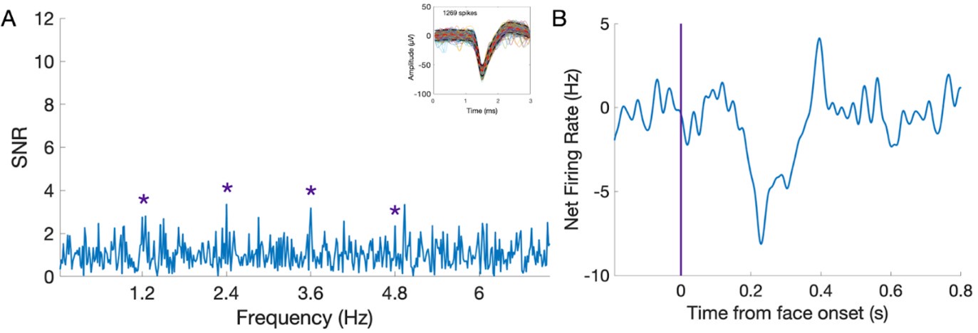
(2) I am not sure how much light the results shed on the physiological basis of the BOLD signal. The authors write that the results reveal "that BOLD decreases can be due to relative, but also absolute, spike suppression in the human brain" (line 120). But I think to make this claim, you would need a region that exclusively had neurons showing absolute suppression, not a region with a mix of neurons, some showing absolute suppression and some showing relative suppression, as here. The responses of both groups of neurons contribute to the measured BOLD signal, so it seems impossible to tell from these data how absolute suppression per se drives the BOLD response.
It is a fact that we find both kinds of responses in the same region. We cannot tell with this technique if neurons showing relative vs. absolute suppression of responses are spatially segregated for instance (e.g., forming two separate sub-regions) or are intermingled. And we cannot tell from our data how absolute suppression per se drives the BOLD response. In our view, this does not diminish the interest and originality of the study, but the statement "that BOLD decreases can be due to relative, but also absolute, spike suppression in the human brain” has been rephrased in the revised manuscript: "that BOLD decreases can be due to relative, or absolute (or a combination of both), spike suppression in the human brain”.
Reviewer #3 (Public review):
In this paper the authors conduct two experiments an fMRI experiment and intracranial recordings of neurons in two patients P1 and P2. In both experiments, they employ a SSVEP paradigm in which they show images at a fast rate (e.g. 6Hz) and then they show face images at a slower rate (e.g. 1.2Hz), where the rest of the images are a variety of object images. In the first patient, they record from neurons over a region in the mid fusiform gyrus that is face-selective and in the second patient, they record neurons from a region more medially that is not face selective (it responds more strongly to objects than faces). Results find similar selectivity between the electrophysiology data and the fMRI data in that the location which shows higher fMRI to faces also finds face-selective neurons and the location which finds preference to non faces also shows non face preferring neurons.
Strengths:
The data is important in that it shows that there is a relationship between category selectivity measured from electrophysiology data and category-selective from fMRI. The data is unique as it contains a lot of single and multiunit recordings (245 units) from the human fusiform gyrus - which the authors point out - is a humanoid specific gyrus.
Weaknesses:
My major concerns are two-fold:
(i) There is a paucity of data; Thus, more information (results and methods) is warranted; and in particular there is no comparison between the fMRI data and the SEEG data.
We thank reviewer #3 for their positive evaluation of our paper. If the reviewer means paucity of data presentation, we agree and we provide more presentation below, although the methods and results information appear as complete to us. The comparison between fMRI and SEEG is there, but can only be indirect (i.e., collected at different times and not related on a trial-by-trial basis for instance). In addition, our manuscript aims at providing a short empirical contribution to further our understanding of the relationship between neural responses and BOLD signal, not to provide a model of neurovascular coupling.
(ii) One main claim of the paper is that there is evidence for suppressed responses to faces in the non-face selective region. That is, the reduction in activation to faces in the non-face selective region is interpreted as a suppression in the neural response and consequently the reduction in fMRI signal is interpreted as suppression. However, the SSVEP paradigm has no baseline (it alternates between faces and objects) and therefore it cannot distinguish between lower firing rate to faces vs suppression of response to faces.
We understand the concern of the reviewer, but we respectfully disagree that our paradigm cannot distinguish between lower firing rate to faces vs. suppression of response to faces. Indeed, since the stimuli are presented periodically (6 Hz), we can objectively distinguish stimulus-related activity from spontaneous neuronal firing. The baseline corresponds to spikes that are non-periodic, i.e., unrelated to the (common face and object) stimulation. For a subset of neurons, even this non-periodic baseline activity is suppressed, above and beyond the suppression of the 6 Hz response illustrated on Figure 2. We mention it in the manuscript, but we agree that we do not present illustrations of such decrease in the time-domain for SU, which we did not consider as being necessary initially (please see below for such presentation).
(1) Additional data: the paper has 2 figures: figure 1 which shows the experimental design and figure 2 which presents data, the latter shows one example neuron raster plot from each patient and group average neural data from each patient. In this reader's opinion this is insufficient data to support the conclusions of the paper. The paper will be more impactful if the researchers would report the data more comprehensively.
We answer to more specific requests for additional evidence below, but the reviewer should be aware that this is a short report, which reaches the word limit. In our view, the group average neural data should be sufficient to support the conclusions, and the example neurons are there for illustration. And while we cannot provide the raster plots for a large number of neurons, the anonymized data is made available at:
(a) There is no direct comparison between the fMRI data and the SEEG data, except for a comparison of the location of the electrodes relative to the statistical parametric map generated from a contrast (Fig 2a,d). It will be helpful to build a model linking between the neural responses to the voxel response in the same location - i.e., estimate from the electrophysiology data the fMRI data (e.g., Logothetis & Wandell, 2004).
As mentioned above the comparison between fMRI and SEEG is indirect (i.e., collected at different times and not related on a trial-by-trial basis for instance) and would not allow to make such a model.
(b) More comprehensive analyses of the SSVEP neural data: It will be helpful to show the results of the frequency analyses of the SSVEP data for all neurons to show that there are significant visual responses and significant face responses. It will be also useful to compare and quantify the magnitude of the face responses compared to the visual responses.
The data has been analyzed comprehensively, but we would not be able to show all neurons with such significant visual responses and face-selective responses.
(c) The neuron shown in E shows cyclical responses tied to the onset of the stimuli, is this the visual response?
Correct, it’s the visual response at 6 Hz.
If so, why is there an increase in the firing rate of the neuron before the face stimulus is shown in time 0?
Because the stimulation is continuous. What is displayed at 0 is the onset of the face stimulus, with each face stimulus being preceded by 4 images of nonface objects.
The neuron's data seems different than the average response across neurons; This raises a concern about interpreting the average response across neurons in panel F which seems different than the single neuron responses
The reviewer is correct, and we apologize for the confusion. This is because the average data on panel F has been notch-filtered for the 6 Hz (and harmonic responses), as indicated in the methods (p.11): ‘a FFT notch filter (filter width = 0.05 Hz) was then applied on the 70 s single or multi-units time-series to remove the general visual response at 6 Hz and two additional harmonics (i.e., 12 and 18 Hz)’.
Here is the same data without the notch-filter (the 6Hz periodic response is clearly visible):
Author response image 2.
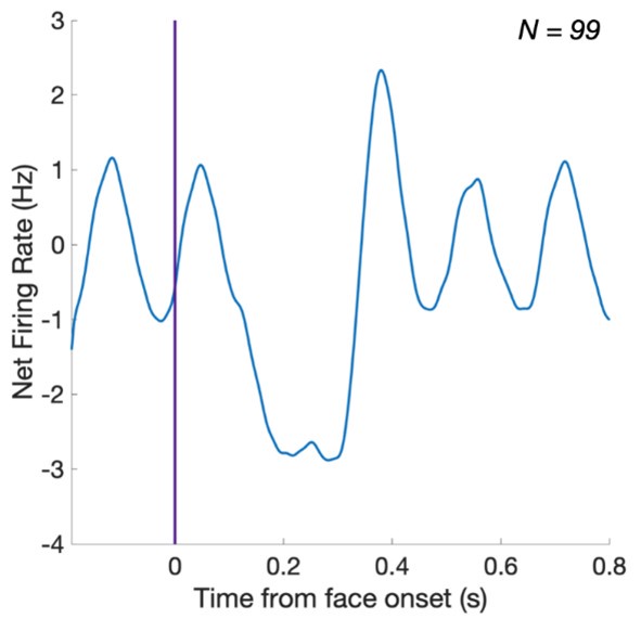
For sake of clarity, we prefer presenting the notch-filtered data in the paper, but the revised version makes it clear in the figure caption that the average data has been notch-filtered.
(d) Related to (c) it would be useful to show raster plots of all neurons and quantify if the neural responses within a region are homogeneous or heterogeneous. This would add data relating the single neuron response to the population responses measured from fMRI. See also Nir 2009.
We agree with the reviewer that this is interesting, but again we do not think that it is necessary for the point made in the present paper. Responses in these regions appear rather heterogenous, and we are currently working on a longer paper with additional SEEG data (other patients tested for shorter sessions) to define and quantify the face-selective neurons in the MidFusiform gyrus with this approach (without relating it to the fMRI contrast as reported here).
(e) When reporting group average data (e.g., Fig 2C,F) it is necessary to show standard deviation of the response across neurons.
We agree with the reviewer and have modified Figure 2 accordingly in the revised manuscript.
(f) Is it possible to estimate the latency of the neural responses to face and object images from the phase data? If so, this will add important information on the timing of neural responses in the human fusiform gyrus to face and object images.
The fast periodic paradigm to measure neural face-selectivity has been used in tens of studies since its original reports:
in EEG: Rossion et al., 2015: https://doi.org/10.1167/15.1.18
in SEEG: Jonas et al., 2016: https://doi.org/10.1073/pnas.1522033113
In this paradigm, the face-selective response spreads to several harmonics (1.2 Hz, 2.4 Hz, 3.6 Hz, etc.) (which are summed for quantifying the total face-selective amplitude). This is illustrated below by the averaged single units’ SNR spectra across all recording sessions for both participants.
Author response image 3.
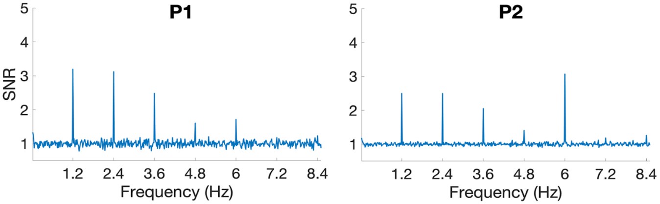
There is no unique phase-value, each harmonic being associated with a phase-value, so that the timing cannot be unambiguously extracted from phase values. Instead, the onset latency is computed directly from the time-domain responses, which is more straightforward and reliable than using the phase. Note that the present paper is not about the specific time-courses of the different types of neurons, which would require a more comprehensive report, but which is not necessary to support the point made in the present paper about the SEEG-fMRI sign relationship.
(g) Related to (e) In total the authors recorded data from 245 units (some single units and some multiunits) and they found that both in the face and nonface selective most of the recoded neurons exhibited face -selectivity, which this reader found confusing: They write “ Among all visually responsive neurons, we found a very high proportion of face-selective neurons (p < 0.05) in both activated and deactivated MidFG regions (P1: 98.1%; N = 51/52; P2: 86.6%; N = 110/127)’. Is the face selectivity in P1 an increase in response to faces and P2 a reduction in response to faces or in both it’s an increase in response to faces
Face-selectivity is defined as a DIFFERENTIAL response to faces compared to objects, not necessarily a larger response to faces. So yes, face-selectivity in P1 is an increase in response to faces and P2 a reduction in response to faces.
Additional methods
(a) it is unclear if the SSVEP analyses of neural responses were done on the spikes or the raw electrical signal. If the former, how is the SSVEP frequency analysis done on discrete data like action potentials?
The FFT is applied directly on spike trains using Matlab’s discrete Fourier Transform function. This function is suitable to be applied to spike trains in the same way as to any sampled digital signal (here, the microwires signal was sampled at 30 kHz, see Methods).
In complementary analyses, we also attempted to apply the FFT on spike trains that had been temporally smoothed by convolving them with a 20ms square window (Le Cam et al., 2023, cited in the paper ). This did not change the outcome of the frequency analyses in the frequency range we are interested in. We have also added one sentence with information in the methods section about spike detection (p.10).
(b) it is unclear why the onset time was shifted by 33ms; one can measure the phase of the response relative to the cycle onset and use that to estimate the delay between the onset of a stimulus and the onset of the response. Adding phase information will be useful.
The onset time was shifted by 33ms because the stimuli are presented with a sinewave contrast modulation (i.e., at 0ms, the stimulus has 0% contrast). 100% contrast is reached at half a stimulation cycle, which is 83.33ms here, but a response is likely triggered before reaching 100% contrast. To estimate the delay between the start of the sinewave (0% contrast) and the triggering of a neural response, we tested 7 SEEG participants with the same images presented in FPVS sequences either as a sinewave contrast (black line) modulation or as a squarewave (i.e. abrupt) contrast modulation (red line). The 33ms value is based on these LFP data obtained in response to such sinewave stimulation and squarewave stimulation of the same paradigm. This delay corresponds to 4 screen refresh frames (120 Hz refresh rate = 8.33ms by frame) and 35% of the full contrast, as illustrated below (please see also Retter, T. L., & Rossion, B. (2016). Uncovering the neural magnitude and spatio-temporal dynamics of natural image categorization in a fast visual stream. Neuropsychologia, 91, 9–28).
Author response image 4.
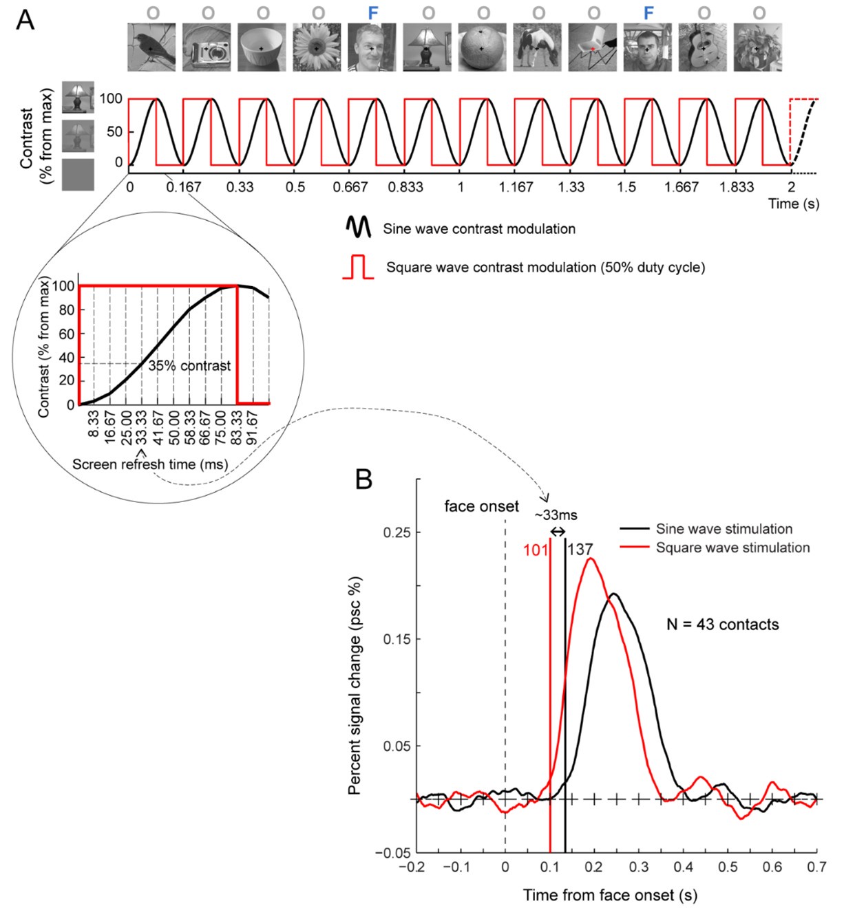
(2) Interpretation of suppression:
The SSVEP paradigm alternates between 2 conditions: faces and objects and has no baseline; In other words, responses to faces are measured relative to the baseline response to objects so that any region that contains neurons that have a lower firing rate to faces than objects is bound to show a lower response in the SSVEP signal. Therefore, because the experiment does not have a true baseline (e.g. blank screen, with no visual stimulation) this experimental design cannot distinguish between lower firing rate to faces vs suppression of response to faces.
The strongest evidence put forward for suppression is the response of non-visual neurons that was also reduced when patients looked at faces, but since these are non-visual neurons, it is unclear how to interpret the responses to faces.
We understand this point, but how does the reviewer know that these are non-visual neurons? Because these neurons are located in the visual cortex, they are likely to be visual neurons that are not responsive to non-face objects. In any case, as the reviewer writes, we think it’s strong evidence for suppression.
We thank all three reviewers for their positive evaluation of our paper and their constructive comments.
Author response:
The following is the authors’ response to the original reviews
Reviewer #1 (Public review):
Summary:
Zhang et al. addressed the question of whether advantageous and disadvantageous inequality aversion can be vicariously learned and generalized. Using an adapted version of the ultimatum game (UG), in three phases, participants first gave their own preference (baseline phase), then interacted with a "teacher" to learn their preference (learning phase), and finally were tested again on their own (transfer phase). The key measure is whether participants exhibited similar choice preferences (i.e., rejection rate and fairness rating) influenced by the learning phase, by contrasting their transfer phase and baseline phase. Through a series of statistical modeling and computational modeling, the authors reported that both advantageous and disadvantageous inequality aversion can indeed be learned (Study 1), and even be generalised (Study 2).
Strengths:
This study is very interesting, it directly adapted the lab's previous work on the observational learning effect on disadvantageous inequality aversion, to test both advantageous and disadvantageous inequality aversion in the current study. Social transmission of action, emotion, and attitude have started to be looked at recently, hence this research is timely. The use of computational modeling is mostly appropriate and motivated. Study 2, which examined the vicarious inequality aversion in conditions where feedback was never provided, is interesting and important to strengthen the reported effects. Both studies have proper justifications to determine the sample size.
Weaknesses:
Despite the strengths, a few conceptual aspects and analytical decisions have to be explained, justified, or clarified.
INTRODUCTION/CONCEPTUALIZATION
(1) Two terms seem to be interchangeable, which should not, in this work: vicarious/observational learning vs preference learning. For vicarious learning, individuals observe others' actions (and optionally also the corresponding consequence resulting directly from their own actions), whereas, for preference learning, individuals predict, or act on behalf of, the others' actions, and then receive feedback if that prediction is correct or not. For the current work, it seems that the experiment is more about preference learning and prediction, and less so about vicarious learning. The intro and set are heavily around vicarious learning, and later the use of vicarious learning and preference learning is rather mixed in the text. I think either tone down the focus on vicarious learning, or discuss how they are different. Some of the references here may be helpful: (Charpentier et al., Neuron, 2020; Olsson et al., Nature Reviews Neuroscience, 2020; Zhang & Glascher, Science Advances, 2020)
We are appreciative of the Reviewer for raising this question and providing the reference. In response to this comment we have elected to avoid, in most cases, use of the term ‘vicarious’ and instead focus the paper on learning of others’ preferences (without specific commitment to various/observational learning per se). These changes are reflected throughout all sections of the revised manuscript, and in the revised title. We believe this simplified terminology has improved the clarity of our contribution.
EXPERIMENTAL DESIGN
(2) For each offer type, the experiment "added a uniformly distributed noise in the range of (-10 ,10)". I wonder what this looks like? With only integers such as 25:75, or even with decimal points? More importantly, is it possible to have either 70:30 or 90:10 option, after adding the noise, to have generated an 80:20 split shown to the participants? If so, for the analyses later, when participants saw the 80:20 split, which condition did this trial belong to? 70:30 or 90:10? And is such noise added only to the learning phase, or also to the baseline/transfer phases? This requires some clarification.
We thank the Reviewer for pointing this out. The uniformly distributed noise was added to all three phases to make the proposers’ behavior more realistic. This added noise was rounded to integer numbers, constrained from -9 to 9, which means in both 70:30 and 90:10 offer types, an 80:20 split could not occur. We have made this feature of our design clear in the Method section Line 524 ~ 528:
“In all task phases, we added uniformly distributed noise to each trial’s offer (ranging from -9 to 9, inclusive, rounding to the nearest integer) such that the random amount added (or subtracted) from the Proposer’s share was subtracted (or added) to the Receiver’s share. We adopted this manipulation to make the proposers’ behavior appear more realistic. The orders of offers participants experienced were fully randomized within each experiment phase. ”
(3) For the offer conditions (90:10, 70:30, 50:50, 30:70, 10:90) - are they randomized? If so, how is it done? Is it randomized within each participant, and/or also across participants (such that each participant experienced different trial sequences)? This is important, as the order especially for the learning phase can largely impact the preference learning of the participants.
We agree with the Reviewer the order in which offers are experienced could be very important. The order of the conditions was randomized independently for each participant (i.e. each participant experienced different trial sequences). We made this point clear in the Methods part. Line 527 ~ 528:
“The orders of offers participants experienced were fully randomized within each experiment phase.”
STATISTICAL ANALYSIS & COMPUTATIONAL MODELING
(4) In Study 1 DI offer types (90:10, 70:30), the rejection rate for DI-AI averse looks consistently higher than that for DI averse (ie, the blue line is above the yellow line). Is this significant? If so, how come? Since this is a between-subject design, I would not anticipate such a result (especially for the baseline). Also, for the LME results (eg, Table S3), only interactions were reported but not the main results.
We thank the Reviewer for pointing out this feature of the results. Prompted by this comment, we compared the baseline rejection rates between two conditions for these two offer types, finding in Experiment 1 that rejection rates in the DI-AI-averse condition were significantly higher than in the DI-averse condition (DI-AI-averse vs. DI-averse; Offer 90:10, β = 0.13, p < 0.001, Offer 70:30, β = 0.09, p < 0.034). We agree with the Reviewer that there should, in principle, be no difference between the experiences of participants in these two conditions is identical in the Baseline phase. However, we did not observe these difference in baseline preferences in Experiment 2 (DI-AI-averse vs. DI-averse; Offer 90:10, β = 0.07, p < 0.100, Offer 70:30, β = 0.05, p < 0.193). On the basis of the inconsistency of this effect across studies we believe this is a spurious difference in preferences stemming from chance.
Regarding the LME results, the reason why only interaction terms are reported is due to the specification of the model and the rationale for testing.
Taking the model reported in Table S3 as an example—a logistic model which examines Baseline phase rejection rates as a function of offer level and condition—the between-subject conditions (DI-averse and DI-AI-averse) are represented by dummy-coded variables. Similarly, offer types were also dummy-coded, such that each of the five columns (90:10, 70:30, 50:50, 30:70, and 10:90) correspond corresponded to a particular offer type. This model specification yields ten interaction terms (i.e., fixed effects) of interest—for example, the “DI-averse × Offer 90:10” indicates baseline rejection rates for 90:10 offers in DI-averse condition. Thus, to compare rejection rates across specific offer types, we estimate and report linear contrasts between these resultant terms. We have clarified the nature of these reported tests in our revised Results—for example, line189-190: “linear contrasts; e.g. 90:10 vs 10:90, all Ps<0.001, see Table S3 for logistic regression coefficients for rejection rates).
Also in response to this comment that and a recommendation from Reviewer 2 (see below), we have revised our supplementary materials to make each model specification clearer as SI line 25:
“RejectionRate ~ 0 + (Disl + Advl):(Offer10 + Offer30 + Offer50 + Offer70 + Offer90) + (1|Subject)”
(5) I do not particularly find this analysis appealing: "we examined whether participants' changes in rejection rates between Transfer and Baseline, could be explained by the degree to which they vicariously learned, defined as the change in punishment rates between the first and last 5 trials of the Learning phase." Naturally, the participants' behavior in the first 5 trials in the learning phase will be similar to those in the baseline; and their behavior in the last 5 trials in the learning phase would echo those at the transfer phase. I think it would be stronger to link the preference learning results to the change between the baseline and transfer phase, eg, by looking at the difference between alpha (beta) at the end of the learning phase and the initial alpha (beta).
Thanks for pointing this out. Also, considering the comments from Reviewer 2 concerning the interpretation of this analysis, we have elected to remove this result from our revision.
(6) I wonder if data from the baseline and transfer phases can also be modeled, using a simple Fehr-Schimdt model. This way, the change in alpha/beta can also be examined between the baseline and transfer phase.
We agree with the Reviewer that a simplified F-S model could be used, in principle, to characterize Baseline and Transfer phase behavior, but it is our view that the rejection rates provide readers with the clearest (and simplest) picture of how participants are responding to inequity. Put another way, we believe that the added complexity of using (and explaining) a new model to characterize simple, steady-state choice behavior (within these phases) would not be justified or add appreciable insights about participants’ behavior.
(7) I quite liked Study 2 which tests the generalization effect, and I expected to see an adapted computational modeling to directly reflect this idea. Indeed, the authors wrote, "[...] given that this model [...] assumes the sort of generalization of preferences between offer types [...]". But where exactly did the preference learning model assume the generalization? In the methods, the modeling seems to be only about Study 1; did the authors advise their model to accommodate Study 2? The authors also ran simulation for the learning phase in Study 2 (Figure 6), and how did the preference update (if at all) for offers (90:10 and 10:90) where feedback was not given? Extending/Unpacking the computational modeling results for Study 2 will be very helpful for the paper.
We are appreciative of the Reviewer’s positive impression of Experiment 2. Upon reflection, we realize that our original submission was not clear about the modeling done in Experiment 2, and we should clarify here that we did also fit the Preference Inference model to this dataset. As in Experiment 1, this model assumes that the participants have a representation of the teacher’s preference as a Fehr-Schmidt form utility function and infer the Teacher’s Envy and Guilt parameters through learning. The model indicates that, on the basis of experience with the Teacher’s preferences on moderately unfair offers (i.e., offer 70:30 and offer 30:70), participants can successfully infer these guess of these two parameters, and in turn, compute Fehr-Schmidt utility to guide their decisions in the extreme unfair offers (i.e., offer 90:10 and offer 10:90).
In response to this comment, we have made this clearer in our Results (Line 377-382):
“Finally, following Experiment 1, we fit a series of computational models of Learning phase choice behavior, comparing the goodness-of-fit of the four best-fitting models from Experiment 1 (see Methods). As before, we found that the Preference Inference model provided the best fit of participants’ Learning Phase behavior (Figure S1a, Table S12). Given that this model is able to infer the Teacher’s underlying inequity-averse preferences (rather than learns offer-specific rejection preferences), it is unsurprising that this model best describes the generalization behavior observed in Experiment 2.”
and in our revised Methods (Line 551-553)
“We considered 6 computational models of Learning Phase choice behavior, which we fit to individual participants’ observed sequences of choices, in both Experiments 1 and 2, via Maximum Likelihood Estimation”
Reviewer #2 (Public review):
Summary:
This study investigates whether individuals can learn to adopt egalitarian norms that incur a personal monetary cost, such as rejecting offers that benefit them more than the giver (advantageous inequitable offers). While these behaviors are uncommon, two experiments demonstrate that individuals can learn to reject such offers through vicarious learning - by observing and acting in line with a "teacher" who follows these norms. The authors use computational modelling to argue that learners adopt these norms through a sophisticated process, inferring the latent structure of the teacher's preferences, akin to theory of mind.
Strengths:
This paper is well-written and tackles a critical topic relevant to social norms, morality, and justice. The findings, which show that individuals can adopt just and fair norms even at a personal cost, are promising. The study is well-situated in the literature, with clever experimental design and a computational approach that may offer insights into latent cognitive processes. Findings have potential implications for policymakers.
Weaknesses:
Note: in the text below, the "teacher" will refer to the agent from which a participant presumably receives feedback during the learning phase.
(1) Focus on Disadvantageous Inequity (DI): A significant portion of the paper focuses on responses to Disadvantageous Inequitable (DI) offers, which is confusing given the study's primary aim is to examine learning in response to Advantageous Inequitable (AI) offers. The inclusion of DI offers is not well-justified and distracts from the main focus. Furthermore, the experimental design seems, in principle, inadequate to test for the learning effects of DI offers. Because both teaching regimes considered were identical for DI offers the paradigm lacks a control condition to test for learning effects related to these offers. I can't see how an increase in rejection of DI offers (e.g., between baseline and generalization) can be interpreted as speaking to learning. There are various other potential reasons for an increase in rejection of DI offers even if individuals learn nothing from learning (e.g. if envy builds up during the experiment as one encounters more instances of disadvantageous fairness).
We are appreciative of the Reviewer’s insight here and for the opportunity to clarify our experimental logic. We included DI offers in order to 1) expose participants to the full spectrum of offer types, and avoid focusing participants exclusively upon AI offers, which might result in a demand characteristic and 2) to afford exploration of how learning dynamics might differ in DI context s—which was, to some extent, examined in our previous study (FeldmanHall, Otto, & Phelps, 2018)—versus AI contexts. Furthermore, as this work builds critically on our previous study, we reasoned that replicating these original findings (in the DI context) would be important for demonstrating the generality of the learning effects in the DI context across experimental settings. We now remark on this point in our revised Introduction Line 129 ~132:
“In addition, to mechanistically probe how punitive preferences are acquired in Adv-I and Dis-I contexts—in turn, assessing the replicability of our earlier study investigating punitive preference acquisition in the Dis context—we also characterize trial-by-trial acquisition of punitive behavior with computational models of choice.”
(2) Statistical Analysis: The analysis of the learning effects of AI offers is not fully convincing. The authors analyse changes in rejection rates within each learning condition rather than directly comparing the two. Finding a significant effect in one condition but not the other does not demonstrate that the learning regime is driving the effect. A direct comparison between conditions is necessary for establishing that there is a causal role for the learning regime.
We agree with the Reviewer and upon reflection, believe that direct comparisons between conditions would be helpful to support the claim that the different learning conditions are responsible for the observed learning effects. In brief, these specific tests buttress the idea that exposure to AI-averse preferences result in increases in AI punishment rates in the Transfer phase (over and above the rates observed for participants who were only exposed to DI-averse preferences).
Accordingly, our revision now reports statistics concerning the differences between conditions for AI offers in Experiment 1 (Line 198~ 207):
“Importantly, when comparing these changes between the two learning conditions, we observed significant differences in rejection rates for Adv-I offers: compared to exposure to a Teacher who rejected only Dis-I offers, participants exposed to a Teacher who rejected both Dis-I and Adv-I offers were more likely to reject Adv-I offers and rated these offers more unfair. This difference between conditions was evident in both 30:70 offers (Rejection rates: β(SE) = 0.10(0.04), p = 0.013; Fairness ratings: β(SE) = -0.86(0.17), p < 0.001) and 10:90 offers (Rejection rates: β(SE) = 0.15(0.04), p < 0.001, Fairness ratings: β(SE) = -1.04(0.17), p < 0.001). As a control, we also compared rejection rates and fairness rating changes between conditions in Dis-I offers (90:10 and 30:70) and Fair offers (i.e., 50:50) but observed no significant difference (all ps > 0.217), suggesting that observing an Adv-I-averse Teacher’s preferences did not influence participants’ behavior in response to Dis-I offers.”
Line 222 ~ 230:
“A mixed-effects logistic regression revealed a significant larger (positive) effect of trial number on rejection rates of Adv-I offers for the Adv-Dis-I-Averse condition compared to the Dis-I-Averse condition. This relative rejection rate increase was evident both in 30:70 offers (Table S7; β(SE) = -0.77(0.24), p < 0.001) and in 10:90 offers (β(SE) = -1.10(0.33), p < 0.001). In contrast, comparing Dis-I and Fairness offers when the Teacher showed the same tendency to reject, we found no significant difference between the two conditions (90:10 splits: β(SE)=-0.48(0.21),p=0.593;70:30 splits: β(SE)=-0.01(0.14),p=0.150; 50:50 splits: β(SE)=-0.00(0.21),p=0.086). In other words, participants by and large appeared to adjust their rejection choices in accordance with the Teacher’s feedback in an incremental fashion.”
And in Experiment 2 Line 333 ~ 345:
“Similar to what we observed in Experiment 1 (Figure 4a), Compared to the participants in the Dis-I-Averse Condition, participants in the Adv-I-Averse Condition increased their rates of rejection of extreme Adv-I offerers (i.e., 10:90) in the Transfer Phase, relative to the Baseline phase (β(SE) = -0.12(0.04), p < 0.004; Table S9), suggesting that participants’ learned (and adopted) Adv-I-averse preferences, generalized from one specific offer type (30:70) to an offer types for which they received no Teacher feedback (10:90). Examining extreme Dis-I offers where the Teacher exhibited identical preferences across the two learning conditions, we found no difference in the Changes of Rejection Rates from Baseline to Transfer phase between conditions (β(SE) = -0.05(0.04), p < 0.259). Mirroring the observed rejection rates (Figure 4b), relative to the Dis-I-Averse Condition, participants’ fairness ratings for extreme Adv-I offers increased more from the Baseline to Transfer phase in the Adv-Dis-I-Averse Condition than in the Dis-I-Averse condition (β(SE) = -0.97(0.18), p < 0.001), but, importantly, changes in fairness ratings for extreme Dis-I offers did not differ significantly between learning conditions (β(SE) = -0.06(0.18), p < 0.723)”
Line 361 ~ 368:
“Examining the time course of rejection rates in Adv-I-contexts during the Learning phase (Figure 5) revealed that participants learned over time to punish mildly unfair 30:70 offers, and these punishment preferences generalized to more extreme offers (10:90). Specifically, compared to the Dis-I-Averse Condition, in the Adv-Dis-I-Averse condition we observed a significant larger trend of increase in rejections rates for 10:90 (Adv-I) offers (Figure 5, β(SE) = -0.81(0.26), p < 0.002 mixed-effects logistic regression, see Table S10). Again, when comparing the rejection rate increase in the extremely Dis-I offers (90:10), we didn’t find significant difference between conditions (β(SE) = -0.25(0.19), p < 0.707).”
(3) Correlation Between Learning and Contagion Effects:
The authors argue that correlations between learning effects (changes in rejection rates during the learning phase) and contagion effects (changes between the generalization and baseline phases) support the idea that individuals who are better aligning their preferences with the teacher also give more consideration to the teacher's preferences later during generalization phase. This interpretation is not convincing. Such correlations could emerge even in the absence of learning, driven by temporal trends like increasing guilt or envy (or even by slow temporal fluctuations in these processes) on behalf of self or others. The reason is that the baseline phase is temporally closer to the beginning of the learning phase whereas the generalization phase is temporally closer to the end of the learning phase. Additionally, the interpretation of these effects seems flawed, as changes in rejection rates do not necessarily indicate closer alignment with the teacher's preferences. For example, if the teacher rejects an offer 75% of the time then a positive 5% learning effect may imply better matching the teacher if it reflects an increase in rejection rate from 65% to 70%, but it implies divergence from the teacher if it reflects an increase from 85% to 90%. For similar reasons, it is not clear that the contagion effects reflect how much a teacher's preferences are taken into account during generalization.
This comment is very similar to a previous comment made by Reviewer 1, who also called into question the interpretability of these correlations. In response to both of these comments we have elected to remove these analyses from our revision.
(4) Modeling Efforts: The modelling approach is underdeveloped. The identification of the "best model" lacks transparency, as no model-recovery results are provided, and fits for the losing models are not shown, leaving readers in the dark about where these models fail. Moreover, the reinforcement learning (RL) models used are overly simplistic, treating actions as independent when they are likely inversely related (for example, the feedback that the teacher would have rejected an offer provides feedback that rejection is "correct" but also that acceptance is "an error", and the later is not incorporated into the modelling). It is unclear if and to what extent this limits current RL formulations. There are also potentially important missing details about the models. Can the authors justify/explain the reasoning behind including these variants they consider? What are the initial Q-values? If these are not free parameters what are their values?
We are appreciative of the Reviewer for identifying these potentially unaddressed questions.
The RL models we consider in the present study are naïve models which, in our previous study (FeldmanHall, Otto, & Phelps, 2018), we found to capture important aspects of learning. While simplistic, we believed these models serve as a reasonable baseline for evaluating more complex models, such as the Preference Inference model. We have made this point more explicit in our revised Introduction, Line 129 ~ 132:
“In addition, to mechanistically probe how punitive preferences may be acquired in Adv-I and Dis-I contexts—in turn, assessing the replicability of our earlier study investigating punitive preference acquisition in the Dis-I context—we also characterize trial-by-trial acquisition of punitive behavior with computational models of choice.”
Again, following from our previous modeling of observational learning (FeldmanHall et al., 2018), we believe that the feedback the Teacher provides here is ideally suited to the RL formalism. In particular, when the teacher indicates that the participant’s choice is what they would have preferred, the model receives a reward of ‘1’ (e.g., the participant rejects and the Teacher indicates they would preferred rejection, resulting in a positive prediction error) otherwise, the model receives a reward of ‘0’ (e.g., the participant accepts and the Teacher indicates they would preferred rejection, resulting in a negative prediction error), indicating that the participant did not choose in accordance with the Teacher’s preferences. Through an error driven learning process, these models provide a naïve way of learning to act in accordance with the Teacher’s preferences.
Regarding the requested model details: When treating the initial values as free parameters (model 5), we set Q(reject, offertype) as free values in [0,1] and Q(accept,offertype) as 0.5. This setting can capture participants' initial tendency to reject or accept offers from this offer type. When the initial values are fixed, for all offer types we set Q(reject, offertype) = Q(accept,offertype) = 0.5. In practice, when the initial values are fixed, setting them to 0.5 or 0 doesn’t make much difference. We have clarified these points in our revised Methods, Line 275 ~ 576:
“We kept the initial values fixed in this model, that is Q<sub>0</sub>(reject,offertype) =0.5, (offertype ∈ 90:10, 70:30, 50:50, 30:70, 10:90)”
And Line 582 ~ 584:
“Formally, this model treats Q<sub>0</sub>(reject,offertype) =0.5, (offertype ∈ 90:10, 70:30, 50:50, 30:70, 10:90) as free parameters with values between 0 and 1.”
(5) Conceptual Leap in Modeling Interpretation: The distinction between simple RL models and preference-inference models seems to hinge on the ability to generalize learning from one offer to another. Whereas in the RL models learning occurs independently for each offer (hence to cross-offer generalization), preference inference allows for generalization between different offers. However, the paper does not explore RL models that allow generalization based on the similarity of features of the offers (e.g., payment for the receiver, payment for the offer-giver, who benefits more). Such models are more parsimonious and could explain the results without invoking a theory of mind or any modelling of the teacher. In such model versions, a learner learns a functional form that allows to predict the teacher's feedback based on said offer features (e.g., linear or quadratic form). Because feedback for an offer modulates the parameters of this function (feature weights) generalization occurs without necessarily evoking any sophisticated model of the other person. This leaves open the possibility that RL models could perform just as well or even show superiority over the preference learning model, casting doubt on the authors' conclusions. Of note: even the behaviourists knew that as Little Albert was taught to fear rats, this fear generalized to rabbits. This could occur simply because rabbits are somewhat similar to rats. But this doesn't mean little Alfred had a sophisticated model of animals he used to infer how they behave.
We are appreciative of the Reviewer for their suggestion of an alternative explanation for the observed generalization effects. Our understanding of the suggestion, put simply, put simply, is that an RL model could capture the observed generalization effects if the model were to learn and update a functional form of the Teacher’s rejection preferences using an RL-like algorithm. This idea is similar, conceptually to our account of preference learning whereby the learner has a representation of the teacher’s preferences. In our experiment the offer is in the range of [0-100], the crux of this idea is why the participants should take the functional form (either v-shaped or quadratic) with the minimum at 50. This is important because, at the beginning of the learning phase, the rejection rates are already v-shaped with 50 as its minimum. The participants do not need to adjust the minimum of this functional form. Thus, if we assume that the participants represent the teacher’s rejection rate as a v-shape function with a minimum at [50,50], then this very likely implies that the participants have a representation that the teacher has a preference for fairness. Above all, we agree that with suitable setup of the functional form, one could implement an RL model to capture the generalization effects, without presupposing an internal “model” of the teacher’s preferences.
However, there is another way of modeling the generalization effect by truly “model-free” similarity-based Reinforcement learning. In this approach, we do not assume any particular functional form of the teacher’s preferences, but rather, assumes that experience acquired in one offer type can be generalized to offers that are close (i.e., similar) to the original offer. Accordingly, we implement this idea using a simple RL model in which the action values for each offer type is updated by a learning rate that is scaled by the distance between that offer and the experienced offer (i.e., the offer that generated the prediction error). This learning rate is governed by a Gaussian distribution, similar to the case in the Gaussian process regression (cf. Chulz, Speekenbrink, & Krause, 2018). The initial value of the ‘Reject’ action, for each offer , is set to a free parameter between 0 and 1, and the initial value for the 'Accept’ action was set to 0.5. The results show that even though this model exhibits the trend of increasing rejection rates observed in the AI-DI punish condition, the initial preferences (i.e., starting point of learning) diverges markedly from the Learning phase behavior we observed in Experiment 1:
Author response image 1.
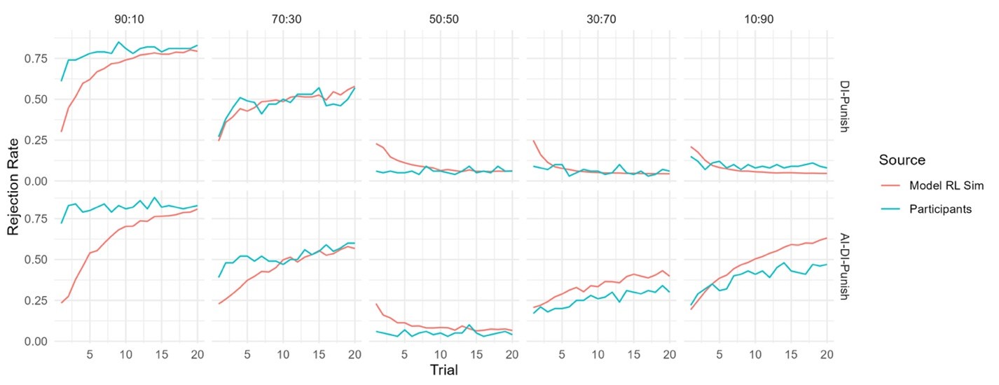
This demonstrated that the participant at least maintains a representation of the teacher’s preference at the beginning. That is, they have prior knowledge about the shape of this preference. We incorporated this property into the model, that is, we considered a new model that assumes v-shaped starting values for rejection with two parameters, alpha and beta, governing the slope of this v-shaped function (this starting value actually mimics the shape of the preference functions of the Fehr-Schmidt model). We found that this new model (which we term the “Model RL Sim Vstart”) provided a satisfactory qualitative fit of the Transfer phase learning curves in Experiment 1 (see below).
Author response image 2.
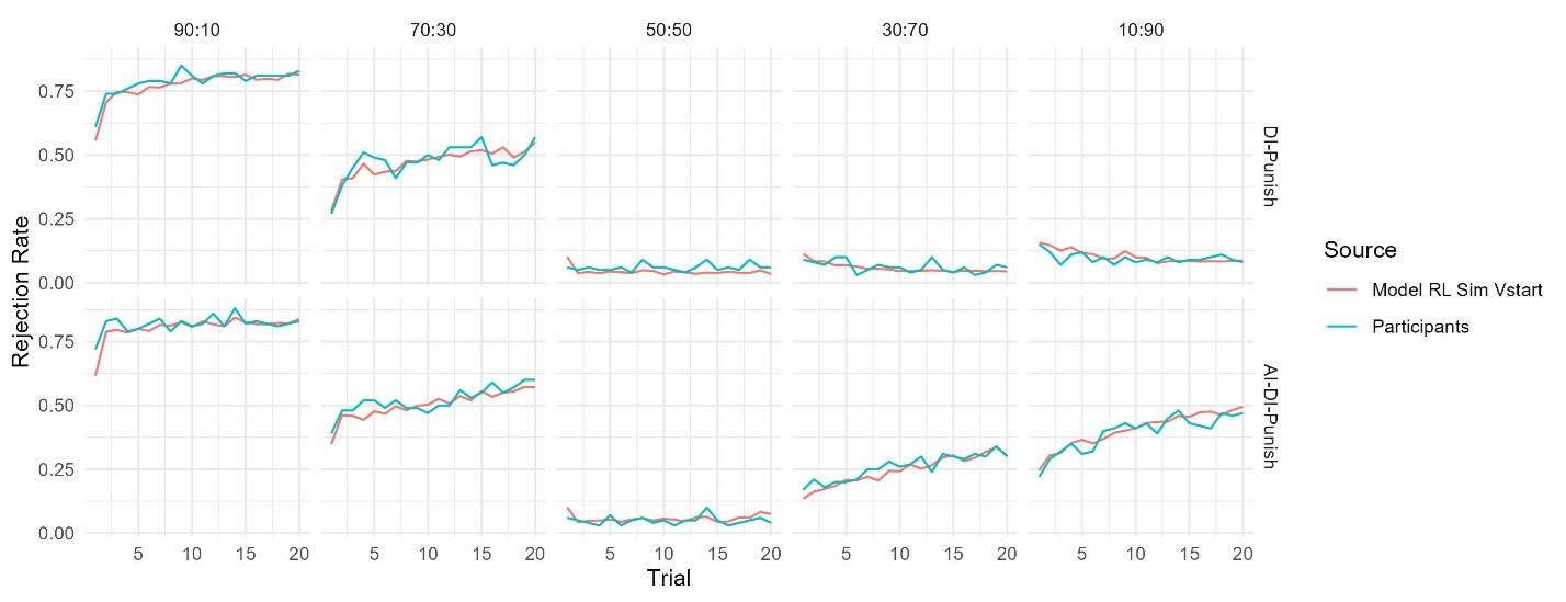
However, we didn’t adopt this model as the best model for the following reasons. First, this model yielded a larger AIC value (indicating worse quantitative fit) compared to our preference Inference model in both Experiments 1 and 2, likely owing to its increased complexity (5 free parameters versus 4 in the Preference Inference model). Accordingly, we believe that inclusion of this model in our revised submission would be more distracting than helpful on account of the added complexity of explaining and justifying these assumptions, and of course its comparatively poor goodness of fit (relative to the preference inference model).
(6) Limitations of the Preference-Inference Model: The preference-inference model struggles to capture key aspects of the data, such as the increase in rejection rates for 70:30 DI offers during the learning phase (e.g. Figure 3A, AI+DI blue group). This is puzzling.
Thinking about this I realized the model makes quite strong unintuitive predictions that are not examined. For example, if a subject begins the learning phase rejecting the 70:30 offer more than 50% of the time (meaning the starting guilt parameter is higher than 1.5), then overleaning the tendency to reject will decrease to below 50% (the guilt parameter will be pulled down below 1.5). This is despite the fact the teacher rejects 75% of the offers. In other words, as learning continues learners will diverge from the teacher. On the other hand, if a participant begins learning to tend to accept this offer (guilt < 1.5) then during learning they can increase their rejection rate but never above 50%. Thus one can never fully converge on the teacher. I think this relates to the model's failure in accounting for the pattern mentioned above. I wonder if individuals actually abide by these strict predictions. In any case, these issues raise questions about the validity of the model as a representation of how individuals learn to align with a teacher's preferences (given that the model doesn't really allow for such an alignment).
In response to this comment we explain our efforts to build a new model that might be able conceptually resolves the issue identified by the Reviewer.
The key intuition guiding the Preference inference model is a Bayesian account of learning which we aimed to further simplify. In this setting, a Bayesian learner maintains a representation of the teacher’s inequity aversion parameters and updates it according to the teacher’s (observed) behavior. Intuitively, the posterior distribution shifts to the likelihood of the teacher’s action. On this view, when the teacher rejects, for instance, an AI offer, the learner should assign a higher probability to larger values of the Guilt parameter, and in turn the learner should change their posterior estimate to better capture the teacher’s preferences.
In the current study, we simplified this idea, implementing this sort of learning using incremental “delta rule” updating (e.g. Equation 8 of the main text). Then the key question is to define the “teaching signal”. Assuming that the teacher rejects an offer 70:30, based on Bayesian reasoning, the teacher’s envy parameter (α) is more likely to exceed 1.5 (computed as 30/(50-30), per equation 7) than to be smaller than 1.5. Thus, 1.5, which is then used in equation 8 to update α, can be thought of as a teaching signal. We simply assumed that if the initial estimate is already greater than 1.5, which means the prior is consistent with the likelihood, no updating would occur. This assumption raises the question of how to set the learning rate range. In principle, an envy parameter that is larger than 1.5 should be the target of learning (i.e., the teaching signal), and thus our model definition allows the learning rate to be greater than 1, incorporating this possibility.
Our simplified preference inference model has already successfully captured some key aspects of the participants’ learning behavior. However, it may fail in the following case: assume that the participant has an initial estimate of 1.51 for the envy parameter (β). Let’s say this corresponds to a rejection rate of 60%. Thus, no matter how many times the teacher rejects the offer 70:30, the participant’s estimate of the envy parameter remains the same, but observing only one offer acceptance would decrease this estimate, and in turn, would decrease the model’s predicted rejection rate. We believe this is the anomalous behavior—in 70:30 offers—identified by the Reviewer which the model does not appear able to recreate participants’ in these offers.
This issue actually touches the core of our model specification, that is, the choosing of the teaching signal. As we chose 1.5 as the teaching signal—i.e. lower bound on whenever the teacher rejects or accepts an offer of 70:30, a very small deviation of 1.5 would fail one part of updating. One way to mitigate this problem would be to choose a lower bound for α greater than 1.5, such that when the Teacher rejects a 70:30 offer, we assign a number greater than 1.5 (by ‘hard-coding’ this into the model via modification of equation 7). One sensible candidate value could be the middle point between 1.5 and 10 (the maximum value of α per our model definition). Intuitively, the model of this setting could still pull up the value of α to 1.51 when the teacher rejects 70:30, thus alleviating (but not completely eliminating) the anomaly.
We fitted this modified Preference Inference model to the data from Experiment 1 (see Author response image 3 below) and found that even though this model has a smaller AIC (and thus better quantitative fit than the original Preference Inference model), it still doesn’t fully capture the participants’ behavior for 70:30 offers.
Author response image 3.
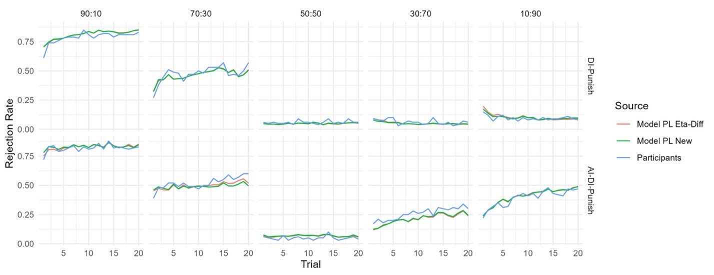
Accordingly, rather than revising our model to include an unprincipled ‘kludge’ to account for this minor anomaly in the model behavior, we have opted to report our original model in our revision as we still believe it parsimoniously captures our intuitions about preference learning and provides a better fit to the observed behavior than the other RL models considered in the present study.
Reviewer #1 (Recommendations for the authors):
(1) I do not particularly prefer the acronyms AI and DI for disadvantageous inequity and advantageous inequity. Although they have been used in the literature, not every single paper uses them. More importantly, AI these days has such a strong meaning of artificial intelligence, so when I was reading this, I'd need to very actively inhibit this interpretation. I believe for the readability for a wider readership of eLife, I would advise not to use AI/DI here, but rather use the full terms.
We thank the Reviewer for this suggestion. As the full spelling of the two terms are somewhat lengthy, and appear frequently in the figures, we have elected to change the abbreviations for disadvantageous inequity and advantageous inequity to Dis-I and Adv-I, respectively in the main text and the supplementary information. We still use AI/DI in the response letter to make the terminology consistent.
(2) Do "punishment rate" and "rejection rate" mean the same? If so, it would be helpful to stick with one single term, eg, rejection rate.
We thank the Reviewer for this suggestion. As these terms have the same meaning, we have opted to use the term “rejection rate” throughout the main text.
(3) For the linear mixed effect models, were other random effect structures also considered (eg, random slops of experimental conditions)? It might be worth considering a few model specifications and selecting the best one to explain the data.
Thanks for this comment. Following established best practices (Barr, Levy, Scheepers, & Tily, 2013) we have elected to use a maximal random effects structure, whereby all possible predictor variables in the fixed effects structure also appear in the random effects structure.
(4) For equation (4), the softmax temperature is denoted as tau, but later in the text, it is called gamma. Please make it consistent.
We are appreciative of the Reviewer’s attention to detail. We have corrected this error.
Reviewer #2 (Recommendations for the authors):
(1) Several Tables in SI are unclear. I wasn't clear if these report raw probabilities of coefficients of mixed models. For any mixed models, it would help to give the model specification (e.g., Walkins form) and explain how variables were coded.
We are appreciative of the Reviewer’s attention to detail. We have clarified, in the captions accompanying our supplemental regression tables, that these coefficients represent log-odds. Regretfully we are unaware of the “Walkins form” the Reviewer references (even after extensive searching of the scientific literature). However, in our new revision we do include lme4 model syntax in our supplemental information which we believe will be helpful for readers seeking replicate our model specification.
(2) In one of the models it was said that the guilt and envy parameters were bounded between 0-1 but this doesn't make sense and I think values outside this range were later reported.
We are again appreciative of the Reviewer’s attention to detail. This was an error we have corrected— the actual range is [0,10].
(3) It is unclear if the model parameters are recoverable.
In response to this comment our revision now reports a basic parameter recovery analysis for the winning Preference Inference model. This is reported in our revised Methods:
“Finally, to verify if the free parameters of the winning model (Preference Inference) are recoverable, we simulated 200 artificial subjects, based on the Learning Phase of Experiment 1, with free parameters randomly chosen (uniformly) from their defined ranges. We then employed the same model-fitting procedure as described above to estimate these parameter value, observing that parameters. We found that all parameters of the model can be recovered (see Figure S2).”
And scatter plots depicting these simulated (versus recovered) parameters are given in Figure S2 of our revised Supplementary Information:
(4) I was confused about what Figure S2 shows. The text says this is about correlating contagious effects for different offers but the captions speak about learning effects. This is an important aspect which is unclear.
We have removed this figure in response to both Reviewers’ comments about the limited insights that can be drawn on the basis of these correlations.
Synthèse sur les Événements Traumatiques et le Secourisme en Santé Mentale
Résumé
Ce document de synthèse analyse en profondeur la nature des événements traumatiques, le trouble de stress post-traumatique (TSPT) et le rôle crucial des secouristes en santé mentale.
S'appuyant sur des expertises psychiatriques et des témoignages de terrain, il ressort que la compréhension du traumatisme repose sur la distinction fondamentale entre le stress aigu, une réaction adaptative normale, et le TSPT, un trouble chronique pouvant se manifester des mois après l'événement.
L'intervention d'un secouriste PSSM (Premiers Secours en Santé Mentale) est essentielle pour créer un climat de sécurité, d'écoute non-jugeante et de réassurance.
Les études de cas de Fabienne, assistante sociale, et de Laurine, une jeune femme aidant une amie, démontrent l'application pratique des compétences PSSM :
sont des piliers de l'intervention.
Le secouriste agit comme un maillon essentiel, guidant la personne en souffrance vers des ressources professionnelles adaptées (thérapies comme l'EMDR, centres médico-psychologiques), tout en apprenant à gérer son propre stress et à reconnaître les limites de son rôle.
La formation PSSM est présentée comme une démarche citoyenne indispensable pour briser les tabous et outiller chacun à apporter un premier soutien efficace.
--------------------------------------------------------------------------------
Un événement est considéré comme potentiellement traumatique lorsqu'il confronte une personne, directement ou indirectement, à la mort, à une menace de mort, à la peur de mourir, à de graves blessures ou à une menace pour son intégrité physique ou celle d'un tiers.
• Caractéristiques : Il provoque généralement une détresse intense, un sentiment d'impuissance et d'horreur.
• Exemples : Actes de violence interpersonnelle (viols, agressions), accidents, catastrophes naturelles, guerres, attentats, actes de torture.
• Statistiques clés (selon l'OMS) :
◦ 70 % des personnes dans le monde vivent un événement potentiellement traumatisant au cours de leur vie. ◦ Environ 4 % de ces personnes sont susceptibles de développer un TSPT.
Le TSPT est un trouble qui peut survenir après un événement traumatique. Il se caractérise par des réactions intenses, désagréables et dysfonctionnelles qui persistent dans le temps.
• Symptômes principaux :
◦ Reviviscence : Flashbacks, cauchemars, intrusions sensorielles.
◦ Évitement : Efforts pour éviter les lieux, personnes ou pensées liés au trauma.
◦ Hypervigilance : État d'alerte constant, irritabilité, sursauts.
◦ Altérations cognitives et de l'humeur : Ruminations, changements d'humeur rapides, sentiment de culpabilité ou de honte.
• Troubles associés : Le TSPT s'accompagne fréquemment de dérégulation émotionnelle, de troubles anxiodépressifs ou de troubles liés à l'usage de substances. Un rétablissement est souvent possible avec une prise en charge adaptée.
Selon le Dr Jean-Michel de Lille, psychiatre, il est crucial de différencier ces deux états :
Caractéristique
Stress Aigu
Trouble de Stress Post-Traumatique (TSPT)
Nature
Réaction adaptative et normale face à un danger imminent.
Trouble chronique et pathologique.
Fonction
Mécanisme de défense (le corps se prépare à fuir ou combattre : cœur qui s'accélère, muscles irrigués).
Le système de stress reste activé longtemps après la disparition du danger.
Durée
Temporaire. La pression redescend en quelques jours ou semaines une fois le danger écarté.
Dure plusieurs mois, voire s'installe durablement. Peut survenir à distance de l'événement (parfois un an après).
Facteurs de risque pour le TSPT
Vulnérabilités génétiques, antécédents de traumatismes infantiles (négligence, abus) qui réactivent un stress plus ancien.
Le Dr de Lille identifie trois principales manières de développer un TSPT, initialement décrites en psychiatrie militaire :
1. Être victime : Avoir subi directement la violence ou l'événement traumatique.
2. Être témoin : Le fait d'être un "témoin impuissant" est une porte d'entrée majeure.
Les taux de TSPT chez les survivants du Bataclan sont plus élevés chez les témoins que chez les victimes directement blessées.
Ce phénomène est aussi crucial chez les enfants témoins de violences conjugales, dont l'impact neuropsychique est décisif.
3. Être auteur : Plus rare, le fait d'avoir commis des actes de violence peut également générer des retours traumatiques.
La reviviscence, ou "intrusion", est l'un des symptômes les plus douloureux du TSPT. La personne revit la scène traumatique de manière involontaire et intense.
• Flashbacks : La scène est revécue y compris physiquement (cœur qui s'accélère, panique) en l'absence de danger objectif.
Ils peuvent être déclenchés par des éléments sensoriels anodins (ex: croiser un homme avec des lunettes si l'agresseur portait des lunettes).
• Cauchemars : Le sommeil est un moment où l'évitement est impossible, les cauchemars ramènent la scène traumatique.
L'exemple est donné d'un jeune militaire hanté des années plus tard par les odeurs d'un charnier qu'il avait dû déterrer, le menant à abuser de morphine et d'alcool pour obtenir un "sommeil anesthétique".
En réaction à la douleur des intrusions, la personne développe des stratégies d'évitement.
• Comportements : Ne plus prendre les transports en commun, éviter le quartier de l'agression, éviter certaines dates (anniversaires).
• Conséquences : Dans les cas sévères, cela peut conduire à un isolement social complet, où toute interaction est perçue comme une menace potentielle.
• Hypervigilance anxieuse : La personne est constamment sur ses gardes, méfiante, a l'impression que le danger va resurgir, ce qui rend la vie "absolument invivable".
Le TSPT affecte profondément la sphère émotionnelle et les relations sociales.
• Culpabilité et Honte : Des sentiments de culpabilité ("pourquoi ai-je survécu et pas d'autres ?") ou de honte (particulièrement dans des métiers où l'expression des émotions est taboue) sont fréquents.
• Irritabilité et Isolement : Comme observé dans le cas de l'agent de la route, la personne peut devenir irritable, s'isoler de ses collègues et de sa famille.
L'intervention d'un secouriste PSSM repose sur des principes clés pour aider une personne suite à un événement traumatique.
1. Créer la Sécurité : L'élément "absolument décisif" est de recréer un climat de sécurité et d'apaisement, de garantir que l'échange se déroule dans un espace sûr.
2. Adopter une Posture Non-Jugeante : Se positionner sur un terrain de parité, d'empathie et de soin, sans se présenter comme un expert.
3. Accueillir et Laisser le Temps : Laisser le temps à la personne d'exprimer ou de ne pas exprimer ses émotions, sans la presser.
La formation PSSM insiste sur cette "notion de temps" et de pauses.
Face à une personne qui revit un événement, le secouriste peut :
• Rassurer sur la culpabilité : Aider la personne à comprendre qu'elle n'est pas coupable de ce qui s'est passé et qu'elle est une personne respectable.
• Écouter activement : Permettre à la personne de verbaliser ce qu'elle a vu, ressenti et comment elle se sent aujourd'hui.
• Réorienter en douceur vers le présent : Lors d'un flashback, introduire gentiment le doute pour aider la personne à faire la part des choses entre la réalité passée (l'agression) et la réalité présente (la sécurité actuelle).
Exemple : "Le monsieur avec des lunettes dans le tram n'est pas celui que vous avez vu il y a des années."
• Informer sur les ressources : Même si la personne n'est pas prête à parler, lui fournir des informations sur les professionnels et les lieux où elle peut trouver de l'aide (plateformes téléphoniques, médecin, etc.).
Le secouriste PSSM n'est pas un professionnel de santé. Il est crucial de reconnaître les limites de son intervention.
Le rôle est d'être un pont, d'accompagner la personne vers une prise en charge adaptée et personnalisée par des professionnels qualifiés.
Fabienne, assistante sociale et secouriste PSSM, est intervenue auprès d'un agent de la route mutique après avoir été confronté à une victime décédée.
Aspect
Description
Contexte
Un agent de la route est en retrait et isolé après avoir été témoin d'un accident mortel.
Le public est majoritairement masculin, peu habitué à parler des émotions, avec un sentiment de "honte" à exprimer sa fragilité.
Défi
L'agent reste silencieux lors des deux premières tentatives d'entretien. Il refuse de se livrer.
Approche PSSM
Fabienne fait preuve d'une grande patience. Elle laisse passer près d'un mois entre la première et la troisième rencontre.
Elle lui fournit des informations sur les ressources dès le deuxième entretien, anticipant un besoin urgent. Lors du troisième entretien (initié par l'agent), elle applique les principes PSSM :
elle prend le temps, accueille les émotions avec une "qualité d'écoute différente", et laisse des temps de pause importants.
Résultat
L'agent parvient enfin à s'exprimer, livrant son mal-être (cauchemars, irritabilité).
Fabienne l'oriente précisément vers un centre médico-psychologique spécialisé. Plus tard, l'agent la remercie pour son aide et sa confiance.
Laurine, secouriste PSSM, a aidé une amie proche, diagnostiquée TSPT suite à une enfance violente, lors d'un flashback.
Aspect
Description
Contexte
L'amie a une enfance marquée par une mère alcoolique et un père violent.
Elle se sent coupable de la mort de ses animaux de compagnie, survenue dans des circonstances troubles.
L'alcool est souvent un "facilitateur d'anxiété" pour elle.
Déclencheur
En sortie de boîte de nuit, la vue d'un chien déclenche une reviviscence intense.
Elle s'effondre en appelant le nom de son chien décédé, persuadée de l'avoir retrouvé.
Intervention
1. Mise en sécurité : Laurine l'isole d'un groupe d'hommes alcoolisés.
Écoute et validation : Elle ne la contredit pas frontalement ("je veux bien te croire qu'il ressemble beaucoup") mais tente de la ramener à la réalité.
Fermeté bienveillante : Face à l'insistance de son amie, elle reste ferme pour la ramener en lieu sûr ("moi en tant qu'amie je peux pas te laisser y retourner").
Réflexion et Résultat
Avec le recul, Laurine pense qu'elle aurait dû être "plus dans l'écoute" et moins dans la volonté de "raisonner".
Le lendemain, elle encourage son amie à en parler à sa psychologue.
L'amie aborde ce trauma en thérapie EMDR et comprend qu'elle a fait un transfert : son désir de sauver le chien était le reflet de son propre désir d'avoir été sauvée enfant.
Le Dr de Lille souligne des avancées majeures dans les thérapies du TSPT, notamment les thérapies d'exposition prolongée.
L'objectif est de permettre à la personne d'évoquer le souvenir traumatique sans subir les symptômes de panique, afin de "désamorcer le couplage" entre la mémoire et la souffrance physique.
• Méthodes psychothérapeutiques :
◦ EMDR (MDR en français) : Thérapie brève utilisant des mouvements oculaires répétitifs pour "digérer" le souvenir traumatique. ◦ ICV (Intégration du Cycle de la Vie)
• Approches pharmacologiques :
◦ Méthode Brunet : Utilisation de bêta-bloquants (ex: Vlocardie) pour diminuer la réaction physique lors de l'évocation.
◦ Expérimentations : Des recherches sont en cours avec de nouvelles molécules comme la MDMA.
Le podcast met en avant plusieurs ressources pour les personnes concernées et les aidants :
• Numéros d'urgence : 112, 15, 18 et le 3114 (numéro national de prévention du suicide).
• PSSM France :
◦ Le site internet pour se former aux premiers secours en santé mentale.
◦ Le "Carnet du secouriste en santé mentale : mieux aider un adulte suite à un événement traumatique" (téléchargement gratuit).
• Centre National de Ressources et de résilience (CN2R) : Chaîne YouTube et témoignages pour améliorer la prise en charge du psychotraumatisme.
• Podcast "Émotion" par Louis Média : L'épisode "Stress post-traumatique : Comment s'inscrit-il dans notre corps ?".
La formation PSSM est décrite comme un outil essentiel qui fournit un "cadre sécurisant" à l'aidant.
Elle permet de savoir quoi faire, mais surtout "ce qu'il ne faut pas faire" et "ne pas dire".
• Elle incite à prendre de la hauteur et à requestionner ses propres pratiques et réflexes.
• Elle aide à gérer son propre stress et à se sentir moins affecté personnellement, ce qui est crucial pour pouvoir aider efficacement sans s'épuiser.
• Pour Fabienne : La formation a enrichi son approche, notamment sur "cette notion du temps" et l'importance de "laisser à l'autre la possibilité ou pas de dire".
• Pour Laurine : La formation lui a permis de trouver un moyen d'avoir du recul, de moins culpabiliser et de prendre conscience du réseau de ressources existant (elle ne connaissait pas PSSM avant).
Le podcast conclut en soulignant que, tout comme les premiers secours physiques, les premiers secours en santé mentale sont une démarche citoyenne.
La formation permet d'acquérir des "clés toutes simples" qui peuvent aider de nombreuses personnes.
Elle encourage chacun à jouer un rôle pour briser les tabous autour des troubles psychiques et à "apprendre à aider".
Samuel Melinao
Ve el vídeo y lee el texto sobre el papel de Samuel Melinao como coordinador de un centro de salud mapuche. ¿Puedes resumir los puntos principales que se mencionan en torno a la medicina mapuche y los problemas a los que se ha enfrentado?
Samuel Melinao Zavala coordina un centro de salud mapuche en La Florida, una comuna en el sur de Santiago.
Ve el vídeo y lee el texto sobre el papel de Samuel Melinao como coordinador de un centro de salud mapuche. ¿Puedes resumir los puntos principales que se mencionan en torno a la medicina mapuche y los problemas a los que se ha enfrentado?
Los estereotipos de los latinoamericanos sobre nosotros mismos
Preguntas de Comprensión
¿Qué etiquetas asigna el artista Martin Vargic a algunos países de América Latina en su ilustración?
¿Cómo se perciben los argentinos según los estereotipos mencionados en el estudio de la Agencia Española de Cooperación Internacional?
¿Qué características positivas se mencionan sobre los brasileños en el estudio de 2006?
¿Cómo se describen los estereotipos sobre los bolivianos en el estudio mencionado?
¿Qué problemas menciona Elier Chara García sobre la falta de información en la propia región?
Preguntas de Reflexión ¿Qué impacto crees que tienen los estereotipos en la percepción de las personas de una región específica? ¿Cómo podríamos combatir la formación y perpetuación de estereotipos negativos entre países?
no todos pueden ser puestos en el mismo saco: "Como uruguayo, siento que muchas veces no se difunde la diversidad latinoamericana y asocian a el ser latino con algo que los uruguayos carecemos totalmente. No bailamos salsa, no somos alegres, somos reservados, y nos gustan estilos musicales que distan mucho de lo tropical",
Explica el significado de la frase "no todos pueden ser puestos en el mismo saco" dentro del contexto y contrasta el ejemplo de Ismael con otro ejemplo propio.
"Por la tendencia de compararnos eternenamente, por un lado con la descendencia europea y por el otro con las raíces indígenas, quedamos atrapados en un limbo de identidad"
¿Puedes explicar esta frase con tus propias palabras y añadir tu opinión al respecto?
aunque la mayoría reconocía poseer muy poca información sobre la historia, la cultura y la forma de vivir de los países sobre los cuales se les estaba preguntando, muchos tenían formada una idea bastante clara sobre sus habitantes.
¿Puedes explicar la ironía contenida en esta frase?
Author Response
The following is the authors’ response to the previous reviews.
Reviewer #1:
Concerns Public Review:
1)The framing of 'infinite possible types of conflict' feels like a strawman. While they might be true across stimuli (which may motivate a feature-based account of control), the authors explore the interpolation between two stimuli. Instead, this work provides confirmatory evidence that task difficulty is represented parametrically (e.g., consistent with literatures like n-back, multiple object tracking, and random dot motion). This parametric encoding is standard in feature-based attention, and it's not clear what the cognitive map framing is contributing.
Suggestion:
1) 'infinite combinations'. I'm frankly confused by the authors response. I don't feel like the framing has changed very much, besides a few minor replacements. Previous work in MSIT (e.g., by the author Zhongzheng Fu) has looked at whether conflict levels are represented similarly across conflict types using multivariate analyses. In the paper mentioned by Ritz & Shenhav (2023), the authors looked at whether conflict levels are represented similarly across conflict types using multivariate analyses. It's not clear what this paper contributes theoretically beyond the connections to cognitive maps, which feel like an interpretative framework rather than a testable hypothesis (i.e., these previous paper could have framed their work as cognitive maps).
Response: We acknowledge the limitations inherent in our experimental design, which prevents us from conducting a strict test of the cognitive space view. In our previous revision, we took steps to soften our conclusions and emphasize these limitations. However, we still believe that our study offers valuable and novel insights into the cognitive space, and the tests we conducted are not merely strawman arguments.
Specifically, our study aimed to investigate the fundamental principles of the cognitive space view, as we stated in our manuscript that “the representations of different abstract information are organized continuously and the representational geometry in the cognitive space is determined by the similarity among the represented information (Bellmund et al., 2018)”. While previous research has applied multivariate analyses to understand cognitive control representation, no prior studies had directedly tested the two key hypotheses associated with cognitive space: (1) that cognitive control representation across conflict types is continuous, and (2) that the similarity among representations of different conflict types is determined by their external similarity.
Our study makes a unique contribute by directly testing these properties through a parametric manipulation of different conflict types. This approach differs significantly from previous studies in two ways. First, our parametric manipulation involves more than two levels of conflict similarity, enabling us to directly test the two critical hypotheses mentioned above. Unlike studies such as Fu et al. (2022) and other that have treated different conflict types categorically, we introduced a gradient change in conflict similarity. This differentiation allowed us to employ representational similarity analysis (RSA) over the conflict similarity, which goes beyond mere decoding as utilized in prior work (see more explanation below for the difference between Fu et al., 2022 and our study [1]).
Second, our parametric manipulation of conflict types differs from previous studies that have manipulated task difficulty, and the modulation of multivariate pattern similarity observed in our study could not be attributed by task difficulty. Previous research, including the Ritz & Shenhav (2023) (see below explanation[2]), has primarily shown that task difficulty modulates univoxel brain activation. A recent work by Wen & Egner (2023) reported a gradual change in the multivariate pattern of brain activations across a wide range of frontoparietal areas, supporting the reviewer’s idea that “task difficulty is represented parametrically”. However, we do not believe that our results reflect the task difficulty representation. For instance, in our study, the spatial Stroop-only and Simon-only conditions exhibited similar levels of difficulty, as indicated by their relatively comparable congruency effects (Fig. S1). Despite this similarity in difficulty, we found that the representational similarity between these two conditions was the lowest (see revised Fig. S4, the most off-diagonal value). This observation aligns more closely with our hypothesis that these two conditions are most dissimilar in terms of their conflict types.
[1] Fu et al. (2022) offers important insights into the geometry of cognitive space for conflict processing. They demonstrated that Simon and flanker conflicts could be distinguished by a decoder that leverages the representational geometry within a multidimensional space. However, their model of cognitive space primarily relies on categorical definitions of conflict types (i.e., Simon versus flanker), rather than exploring a parametric manipulation of these conflict types. The categorical manipulations make it difficult to quantify conceptual similarity between conflict types and hence limit the ability to test whether neural representations of conflict capture conceptual similarity. To the best of our knowledge, no previous studies have manipulated the conflict types parametrically. This gap highlights a broader challenge within cognitive science: effectively manipulating and measuring similarity levels for conflicts, as well as other high-level cognitive processes, which are inherently abstract. We therefore believe our parametric manipulation of conflict types, despite its inevitable limitations, is an important contribution to the literature.
We have incorporated the above statements into our revised manuscript: Methodological implications. Previous studies with mixed conflicts have applied mainly categorical manipulations of conflict types, such as the multi-source interference task (Fu et al., 2022) and color Stroop-Simon task (Liu et al., 2010). The categorical manipulations make it difficult to quantify conceptual similarity between conflict types and hence limit the ability to test whether neural representations of conflict capture conceptual similarity. To the best of our knowledge, no previous studies have manipulated the conflict types parametrically. This gap highlights a broader challenge within cognitive science: effectively manipulating and measuring similarity levels for conflicts, as well as other high-level cognitive processes, which are inherently abstract. The use of an experimental paradigm that permits parametric manipulation of conflict similarity provides a way to systematically investigate the organization of cognitive control, as well as its influence on adaptive behaviors.
[2] The work by Ritz & Shenhav (2023) indeed applied multivariate analyses, but they did not test the representational similarity across different levels of task difficulty in a similar way as our investigation into different levels of conflict types, neither did they manipulated conflict types as our study. They first estimated univariate brain activations that were parametrically scaled by task difficulty (e.g., target coherence), yielding one map of parameter estimates (i.e., encoding subspace) for each of the target coherence and distractor congruence. The multivoxel patterns from the above maps were correlated to test whether the target coherence and distractor congruence share the similar neural encoding. It is noteworthy that the encoding of task difficulty in their study is estimated at the univariate level, like the univariate parametric modulation analysis in our study. The representational similarity across target coherence and distractor congruence was the second-order test and did not reflect the similarity across different difficulty levels. Though, we have found another study (Wen & Egner, 2023) that has directly tested the representational similarity across different levels of task difficulty, and they observed a higher representational similarity between conditions with similar difficulty levels within a wide range of brain regions.
Reference:
Wen, T., & Egner, T. (2023). Context-independent scaling of neural responses to task difficulty in the multiple-demand network. Cerebral Cortex, 33(10), 6013-6027. https://doi.org/10.1093/cercor/bhac479
Fu, Z., Beam, D., Chung, J. M., Reed, C. M., Mamelak, A. N., Adolphs, R., & Rutishauser, U. (2022). The geometry of domain-general performance monitoring in the human medial frontal cortex. Science (New York, N.Y.), 376(6593), eabm9922. https://doi.org/10.1126/science.abm9922
Ritz, H., & Shenhav, A. (2023). Orthogonal neural encoding of targets and distractors supports multivariate cognitive control. https://doi.org/10.1101/2022.12.01.518771 Another issue is suggesting mixtures between two types of conflict may be many independent sources of conflict. Again, this feels like the strawman. There's a difference between infinite combinations of stimuli on the one hand, and levels of feature on the other hand. The issue of infinite stimuli is why people have proposed feature-based accounts, which are often parametric, eg color, size, orientation, spatial frequency. Mixing two forms of conflict is interesting, but the task limitations (i.e., highly correlated features) prevent an analysis of whether these are truly mixed (or eg reflect variations on just one of the conflict types). Without being able to compare a mixture between types vs levels of only one type, it's not clear what you can draw from these results re: how these are combined (and not clear how it reconciles the debate between general and specific).
Response: As the reviewer pointed out, a feature (or a parameterization) is an efficient way to encode potentially infinite stimuli. This is the same idea as our hypothesis: different conflict types are represented in a cognitive space akin to concrete features such as a color spectrum. This concept can be illustrated in the figure below.
Author response image 1.
We would like to clarify that in our study we have manipulated five levels of conflict types, but they all originated from two fundamental sources: vertically spatial Stroop and horizontally Simon conflicts. We agree that the mixture of these two sources does not inherently generate additional conflict sources. However, this mixture does influence the similarity among different conflict conditions, which provides essential variability that is crucial for testing the core hypotheses (i.e., continuity and similarity modulation, see the response above) of the cognitive space view. This clarification is crucial as the reviewer’s impression might have been influenced by our introduction, where we repeatedly emphasized multiple sources of conflicts. Our aim in the introduction was to outline a broader conceptual framework, which might not directly reflect the specific design of our current study. Recognizing the possibility of misinterpretation, we have adjusted our introduction and discussion to place less emphasis on the variety of possible conflict sources. For example, we have removed the expression “The large variety of conflict sources implies that there may be innumerable number of conflict conditions” from the introduction. As we have addressed in the previous response, the observed conflict similarity effect could not be attributed to merely task difficulty. Similarly, the mixture of spatial Stroop and Simon conflicts should not be attributed to one conflict source only; doing so would oversimplify it to an issue of task difficulty, as it would imply that our manipulation of conflict types merely represented varying levels of a single conflict, akin to manipulating task difficulty when everything else being equal. Importantly, the mixed conditions differ from variations along a single conflict source in that they also incorporate components of the other conflict source, thereby introducing difference beyond that would be found within variances of a single conflict source. There are a few additional evidence challenging the single dimension assumption. In our previous revisions, we compared model fittings between the Cognitive-Space model and the Stroop-/Simon-only models, and results showed that the CognitiveSpace model (BIC = 5377093) outperformed the Stroop-Only (BIC = 5377122) and Simon-Only (BIC = 5377096) models. This suggests that mixed conflicts might not be solely reflective of either Stroop or Simon sources, although we did not include these results due to concerns raised by reviewers about the validity of such comparisons, given the high anticorrelation between the two dimensions. Furthermore, Fu et al. (2022) demonstrated that the mixture of Simon and Flanker conflicts (the sf condition) is represented as the vector sum of the Flanker and Simon dimensions within their space model, indicating a compositional nature. Similarly, our mixed conditions are combinations of Stroop and Simon conflicts, and it is plausible that these mixtures represent a fusion of both Stroop and Simon components, rather than just one. Thus, we disagree that the mixture of conflicts is a strawman. In response to this concern, we have included a statement in our limitation section: “Another limitation is that in our design, the spatial Stroop and Simon effects are highly anticorrelated. This constraint may make the five conflict types represented in a unidimensional space (e.g., a circle) embedded in a 2D space. This limitation also means we cannot conclusively rule out the possibility of a real unidimensional space driven solely by spatial Stroop or Simon conflicts. However, this appears unlikely, as it would imply that our manipulation of conflict types merely represented varying levels of a single conflict, akin to manipulating task difficulty when everything else being equal. If task difficulty were the primary variable, we would expect to see greater representational similarity between task conditions of similar difficulty, such as the Stroop and Simon conditions, which demonstrates comparable congruency effects (see Fig. S1). Contrary to this, our findings reveal that the Stroop-only and Simon-only conditions exhibit the lowest representational similarity (Fig. S4). Furthermore, Fu et al. (2022) has shown that the representation of mixtures of Simon and Flanker conflicts was compositional, rather than reflecting single dimension, which also applies to our cases.”
My recommendation would be to dramatically rewrite to reduce the framing of this providing critical evidence in favor of cognitive maps, and being more overt about the limitations of this task. However, the authors are not required to make further revisions in eLife's new model, and it's not clear how my scores would change if they made those revisions (ie the conceptual limitations would remain, the claims would just now match the more limited scope).
Response: With the above rationales and the adjustments we have made in the manuscripts, we believe that we have thoroughly acknowledged and articulated the limitations of our study. Therefore, we have decided against a complete rewrite of the manuscript.
Public Review:
2) The representations within DLPFC appear to treat 100% Stoop and (to a lesser extent) 100% Simon differently than mixed trials. Within mixed trials, the RDM within this region don't strongly match the predictions of the conflict similarity model. It appears that there may be a more complex relationship encoded in this region.
Suggestion:
2) RSMs in the key region of interest. I don't really understand the authors response here either. e.g,. 'It is essential to clarify that our conclusions were based on the significant similarity modulation effect identified in our statistical analysis using the cosine similarity model, where we did not distinguish between the within-Stroop condition and the other four within-conflict conditions (Fig. 7A, now Fig. 8A). This means that the representation of conflict type was not biased by the seemingly disparities in the values shown here'. In Figure 1C, it does look like they are testing this model.
It seems like a stronger validation would test just the mixture trials (i.e., ignoring Simon-only and stroop-only). However, simon/stroop-only conditions being qualitatively different does beg the question of whether these are being represented parametrically vs categorically.
Response: We apologize for the confusion caused by our previous response. To clarify, our conclusions have been drawn based on the robust conflict similarity effect.
The conflict similarity regressor is defined by higher values in the diagonal cells (representing within-conflict similarity) than the off-diagonal cells (indicating between-conflict similarity), as illustrated in Fig. 1C and Fig. 8A (now Fig. 4B). It is important to note that this regressor may not be particularly sensitive to the variations within the diagonal cells. Our previous response aimed to emphasize that the inconsistencies observed along the diagonal do not contradict our core hypothesis regarding the conflict similarity effect.
We recognized that since the visualization in Fig. S4, based on the raw RSM (i.e., Pearson correlation), may have been influenced by other regressors in our model than the conflict similarity effect. To reflect pattern similarity with confounding factors controlled for, we have visualized the RSM by including only the fixed effect of the conflict similarity and the residual while excluding all other factors. As shown in the revised Figure S4, the difference between the within-Stroop and other diagonal cells was greatly reduced. Instead, it revealed a clear pattern where that the diagonal values were higher than the off-diagonal values in the incongruent condition, aligning with our hypothesis regarding the conflict similarity modulator. Although some visual distinctions persist within the five diagonal cells (e.g., in the incongruent condition, the Stroop, Simon, and StMSmM conditions appear slightly lower than StHSmL and StLSmM conditions), follow-up one-way ANOVAs among these five diagonal conditions showed no significant differences. This held true for both incongruent and congruent conditions, with Fs < 1. Thus, we conclude that there is no strong evidence supporting the notion that Simon- and spatial Stroop-only conditions are systematically different from other conflict types. As a result, we decided not to exclude these two conflict types from analysis.
Author response image 2.
The stronger conflict type similarity effect in incongruent versus congruent conditions. Shown are the summary representational similarity matrices for the right 8C region in incongruent (left) and congruent (right) conditions, respectively. Each cell represents the averaged Pearson correlation (after regressing out all factors except the conflict similarity) of cells with the same conflict type and congruency in the 1400×1400 matrix. Note that the seemingly disparities in the values of withinconflict cells (i.e., the diagonal) did not reach significance for either incongruent or congruent trials, Fs < 1.
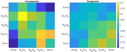
Public Review:
3) To orthogonalized their variables, the authors need to employ a complex linear mixed effects analysis, with a potential influence of implementation details (e.g., high-level interactions and inflated degrees of freedom).
Suggestion:
3) The DF for a mixed model should not be the number of observations minus the number of fixed effects. The gold standard is to use satterthwaite correction (e.g. in Matlab, fixedEffects(lme,'DFMethod','satterthwaite')), or number of subjects - number of fixed effects (i.e. you want to generalize to new subjects, not just new samples from the same subjects). Honestly, running a 4-way interaction probably is probably using more degrees of freedom than are appropriate given the number of subjects.
Response: We concur with the reviewer’s comment that our previous estimation of degrees of freedom (DFs) was inaccurate. Following your suggestion, we have now applied the “Satterthwaite” approach to approximate the DFs for all our linear mixed effect model analyses. This adjustment has led to the correction of both DFs and p values. In the Methods section, we have mentioned this revision.
“We adjusted the t and p values with the degrees of freedom calculated through the Satterthwaite approximation method (Satterthwaite, 1946). Of note, this approach was applied to all the mixed-effect model analyses in this study.”
The application of this method has indeed resulted in a reduction of our statistical significance. However, our overall conclusions remained robust. Instead of the highly stringent threshold used in our previous version (Bonferonni corrected p < .0001), we have now adopted a relatively more lenient threshold of Bonferonni correction at p < 0.05, which is commonly employed in the literature. Furthermore, it is worth noting that the follow-up criteria 2 and 3 are inherently second-order analyses. Criterion 2 involves examining the interaction effect (conflict similarity effect difference between incongruent and congruent conditions), and criterion 3 involves individual correlation analyses. Due to their second-order nature, these criteria inherently have lower statistical power compared to criterion 1 (Blake & Gangestad, 2020). We thus have applied a more lenient but still typically acceptable false discovery rate (FDR) correction to criteria 2 and 3. This adjustment helps maintain the rigor of our analysis while considering the inherent differences in statistical power across the various criteria. We have mentioned this revision in our manuscript:
“We next tested whether these regions were related to cognitive control by comparing the strength of conflict similarity effect between incongruent and congruent conditions (criterion 2) and correlating the strength to behavioral similarity modulation effect (criterion 3). Given these two criteria pertain to second-order analyses (interaction or individual analyses) and thus might have lower statistical power (Blake & Gangestad, 2020), we applied a more lenient threshold using false discovery rate (FDR) correction (Benjamini & Hochberg, 1995) on the above-mentioned regions.”
With these adjustments, we consistently identified similar brain regions as observed in our previous version. Specifically, we found that only the right 8C region met the three criteria in the conflict similarity analysis. In addition, the regions meeting the criteria for the orientation effect included the FEF and IP2 in left hemisphere, and V1, V2, POS1, and PF in the right hemisphere. We have thoroughly revised the description of our results, updated the figures and tables in both the revised manuscript and supplementary material to accurately reflect these outcomes.
Reference:
Blake, K. R., & Gangestad, S. (2020). On Attenuated Interactions, Measurement Error, and Statistical Power: Guidelines for Social and Personality Psychologists. Pers Soc Psychol Bull, 46(12), 1702-1711. https://doi.org/10.1177/0146167220913363
Minor:
- Figure 8 should come much earlier (e.g, incorporated into Figure 1), and there should be consistent terms for 'cognitive map' and 'conflict similarity'.
Response: We appreciate this suggestion. Considering that Figure 7 (“The crosssubject RSA model and the rationale”) also describes the models, we have merged Figure 7 and 8 and moved the new figure ahead, before we report the RSA results. Now you could find it in the new Figure 4, see below. We did not incorporate them into Figure 1 since Figure 1 is already too crowded.
Author response image 3.
Fig. 4. Rationale of the cross-subject RSA model and the schematic of key RSMs. A) The RSM is calculated as the Pearson’s correlation between each pair of conditions across the 35 subjects. For 17 subjects, the stimuli were displayed on the top-left and bottom-right quadrants, and they were asked to respond with left hand to the upward arrow and right hand to the downward arrow. For the other 18 subjects, the stimuli were displayed on the top-right and bottom-left quadrants, and they were asked to respond with left hand to the downward arrow and right hand to the upward arrow. Within each subject, the conflict type and orientation regressors were perfectly covaried. For instance, the same conflict type will always be on the same orientation. To de-correlate conflict type and orientation effects, we conducted the RSA across subjects from different groups. For example, the bottom-right panel highlights the example conditions that are orthogonal to each other on the orientation, response, and Simon distractor, whereas their conflict type, target and spatial Stroop distractor are the same. The dashed boxes show the possible target locations for different conditions. (B) and (C) show the orthogonality between conflict similarity and orientation RSMs. The within-subject RSMs (e.g., Group1-Group1) for conflict similarity and orientation are all the same, but the cross-group correlations (e.g., Group2-Group1) are different. Therefore, we can separate the contribution of these two effects when including them as different regressors in the same linear regression model. (D) and (E) show the two alternative models. Like the cosine model (B), within-group trial pairs resemble betweengroup trial pairs in these two models. The domain-specific model is an identity matrix. The domaingeneral model is estimated from the absolute difference of behavioral congruency effect, but scaled to 0 (lowest similarity) – 1 (highest similarity) to aid comparison. The plotted matrices in B-E include only one subject each from Group 1 and Group 2. Numbers 1-5 indicate the conflict type conditions, for spatial Stroop, StHSmL, StMSmM, StLSmH, and Simon, respectively. The thin lines separate four different sub-conditions, i.e., target arrow (up, down) × congruency (incongruent, congruent), within each conflict type.
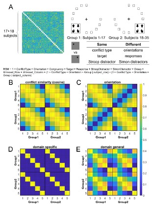
In our manuscript, the term “cognitive map/space” was used when explaining the results in a theoretical perspective, whereas the “conflict similarity” was used to describe the regressor within the RSA. These terms serve distinct purposes in our study and cannot be interchangeably substituted. Therefore, we have retained them in their current format. However, we recognize that the initial introduction of the “Cognitive-Space model” may have appeared somewhat abrupt. To address this, we have included a brief explanatory note: “The model described above employs the cosine similarity measure to define conflict similarity and will be referred to as the Cognitive-Space model.”
Author Response
The following is the authors’ response to the previous reviews.
Thank you and the reviewers for further providing constructive comments and suggestions on our manuscript. On behalf of all the co-authors, I have enclosed a revised version of the above referenced paper. Below, I have merged similar public reviews and recommendations (if applicable) from each reviewer and provided point-by-point responses.
Reviewer #1:
People can perform a wide variety of different tasks, and a long-standing question in cognitive neuroscience is how the properties of different tasks are represented in the brain. The authors develop an interesting task that mixes two different sources of difficulty, and find that the brain appears to represent this mixture on a continuum, in the prefrontal areas involved in resolving task difficulty. While these results are interesting and in several ways compelling, they overlap with previous findings and rely on novel statistical analyses that may require further validation.
Strengths
The authors present an interesting and novel task for combining the contributions of stimulus-stimulus and stimulus-response conflict. While this mixture has been measured in the multi-source interference task (MSIT), this task provides a more graded mixture between these two sources of difficulty.
The authors do a good job triangulating regions that encoding conflict similarity, looking for the conjunction across several different measures of conflict encoding. These conflict measures use several best-practice approaches towards estimating representational similarity.
The authors quantify several salient alternative hypothesis and systematically distinguish their core results from these alternatives.
The question that the authors tackle is important to cognitive control, and they make a solid contribution.
The authors have addressed several of my concerns. I appreciate the authors implementing best practices in their neuroimaging stats.
I think that the concerns that remain in my public review reflect the inherent limitations of the current work. The authors have done a good job working with the dataset they've collected.
Response: We would like to thank the reviewer for the positive evaluation of our manuscript and the constructive comments and suggestions. In response to your suggestions and concerns, we have removed the Stroop/Simon-only and the Stroop+Simon models, revised our conclusion and modified the misleading phrases.
We have provided detailed responses to your comments below.
- The evidence from this previous work for mixtures between different conflict sources makes the framing of 'infinite possible types of conflict' feel like a strawman. The authors cite classic work (e.g., Kornblum et al., 1990) that develops a typology for conflict which is far from infinite. I think few people would argue that every possible source and level of difficulty will have to be learned separately. This work provides confirmatory evidence that task difficulty is represented parametrically (e.g., consistent with the n-back, MOT, and random dot motion literature).
notes for my public concerns.
In their response, the authors say:
'If each combination of the Stroop-Simon combination is regarded as a conflict condition, there would be infinite combinations, and it is our major goal to investigate how these infinite conflict conditions are represented effectively in a space with finite dimensions.'
I do think that this is a strawman. The paper doesn't make a strong case that this position ('infinite combinations') is widely held in the field. There is previous work (e.g., n-back, multiple object tracking, MSIT, dot motion) that has already shown parametric encoding of task difficulty. This paper provides confirmatory evidence, using an interesting new task, that demand are parametric, but does not provide a major theoretical advance.
Response: We agree that the previous expression may have seemed somewhat exaggerative. While it is not “infinite”, recent research indeed suggests that the cognitive control shows domain-specificity across various “domains”, including conflict types (Egner, 2008), sensory modalities (Yang et al., 2017), task-irrelevant stimuli (Spape et al., 2008), and task sets (Hazeltine et al., 2011), to name a few.
These findings collectively support the notion that cognitive control is contextspecific (Bream et al., 2014). That is, cognitive control can be tuned and associated with different (and potentially large numbers of) contexts. Recently, Kikumoto and Mayr (2020) demonstrated that combinations of stimulus, rule and response in the same task formed separatable, conjunctive representations. They further showed that these conjunctive representations facilitate performance. This is in line with the idea that each stimulus-location combination in the present task may be represented separately in a domain-specific manner. Moreover, domain-general task representation can also become domain-specific with learning, which further increases the number of domain-specific conjunctive representations (Mill et al., 2023). In line with the domain-specific account of cognitive control, we referred to the “infinite combinations” in our previous response to emphasize the extreme case of domainspecificity. However, recognizing that the term “infinite” may lead to ambiguity, we have replaced it with phrases such as “a large number of”, “hugely varied”, in our revised manuscript.
We appreciate the reviewer for highlighting the potential connection of our work to existing literature that showed the parametric encoding of task difficulty (e.g., Dagher et al., 1999; Ritz & Shenhav, 2023). For instance, in Ritz et al.’s (2023) study, they parametrically manipulated target difficulty based on consistent ratios of dot color, and found that the difficulty was encoded in the caudal part of dorsal anterior cingulate cortex. Analogically, in our study, the “difficulty” pertains to the behavioral congruency effect that we modulated within the spatial Stroop and Simon dimensions. Notably, we did identify univariate effects in the right dmPFC and IPS associated with the difficulty in the Simon dimension. This parametric effect may lend support to our cognitive space hypothesis, although we exercised caution in interpreting their significance due to the absence of a clear brain-behavioral relevance in these regions. We have added the connection of our work to prior literature in the discussion. The parametric encoding of conflict also mirrors prior research showing the parametric encoding of task demands (Dagher et al., 1999; Ritz & Shenhav, 2023).
However, our analyses extend beyond solely testing the parametric encoding of difficulty. Instead, we focused on the multivariate representation of different conflict types, which we believe is independent from the univariate parametric encoding. Unlike the univariate encoding that relies on the strength within one dimension, the multivariate representation of conflict types incorporates both the spatial Stroop and Simon dimensions. Furthermore, we found that similar difficulty levels did not yield similar conflict representation, as indicated by the low similarity between the spatial Stroop and Simon conditions, despite both showing a similar level of congruency effect (Fig. S1). Additionally, we also observed an interaction between conflict similarity and difficulty (i.e., congruency, Fig. 4B/D), such that the conflict similarity effect was more pronounced when conflict was present. Therefore, we believe that our findings make contribution to the literature beyond the difficulty effect.
Reference:
Egner, T. (2008). Multiple conflict-driven control mechanisms in the human brain. Trends in Cognitive Sciences, 12(10), 374-380. https://doi.org/10.1016/j.tics.2008.07.001
Yang, G., Nan, W., Zheng, Y., Wu, H., Li, Q., & Liu, X. (2017). Distinct cognitive control mechanisms as revealed by modality-specific conflict adaptation effects. Journal of Experimental Psychology: Human Perception and Performance, 43(4), 807-818. https://doi.org/10.1037/xhp0000351
Spapé MM, Hommel B (2008). He said, she said: episodic retrieval induces conflict adaptation in an auditory Stroop task. Psychonomic Bulletin Review,15(6):1117-21. https://doi.org/10.3758/PBR.15.6.1117
Hazeltine E, Lightman E, Schwarb H, Schumacher EH (2011). The boundaries of sequential modulations: evidence for set-level control. Journal of Experimental Psychology: Human Perception & Performance. 2011 Dec;37(6):1898-914. https://doi.org/10.1037/a0024662
Braem, S., Abrahamse, E. L., Duthoo, W., & Notebaert, W. (2014). What determines the specificity of conflict adaptation? A review, critical analysis, and proposed synthesis. Frontiers in Psychology, 5, 1134. https://doi.org/10.3389/fpsyg.2014.01134
Kikumoto A, Mayr U. (2020). Conjunctive representations that integrate stimuli, responses, and rules are critical for action selection. Proceedings of the National Academy of Sciences, 117(19):10603-10608. https://doi.org/10.1073/pnas.1922166117.
Mill, R. D., & Cole, M. W. (2023). Neural representation dynamics reveal computational principles of cognitive task learning. bioRxiv. https://doi.org/10.1101/2023.06.27.546751
Dagher, A., Owen, A. M., Boecker, H., & Brooks, D. J. (1999). Mapping the network for planning: a correlational PET activation study with the Tower of London task. Brain, 122 ( Pt 10), 1973-1987. https://doi.org/10.1093/brain/122.10.1973
Ritz, H., & Shenhav, A. (2023). Orthogonal neural encoding of targets and distractors supports multivariate cognitive control. https://doi.org/10.1101/2022.12.01.518771
- (Public Reviews) The degree of Stroop vs Simon conflict is perfectly negatively correlated across conditions. This limits their interpretation of an integrated cognitive space, as they cannot separately measure Stroop and Simon effects. The author's control analyses have limited ability to overcome this task limitation. While these results are consistent with parametric encoding, they cannot adjudicate between combined vs separated representations.
(Recommendations) I think that it is still an issue that the task's two features (stroop and simon conflict) are perfectly correlated. This fundamentally limits their ability to measure the similarity in these features. The authors provide several control analyses, but I think these are limited.
Response: We need to acknowledge that the spatial Stroop and Simon components in the five conflict conditions were not “perfectly” correlated, with r = –0.89. This leaves some room for the preliminary model comparison to adjudicate between these models. However, it’s essential to note that conclusions based on these results must be tempered. In line with the reviewer’s observation, we agree that the high correlation between the two conflict sources posed a potential limitation on our ability to independently investigate the contribution of spatial Stroop and Simon conflicts. Therefore, in addition to the limitation we have previously acknowledged, we have now further revised our conclusion and adjusted our expressions accordingly.
Specifically, we now regard the parametric encoding of cognitive control not as direct evidence of the cognitive space view but as preliminary evidence that led us to propose this hypothesis, which requires further testing. Notably, we have also modified the title from “Conflicts are represented in a cognitive space to reconcile domain-general and domain-specific cognitive control” to “Conflicts are parametrically encoded: initial evidence for a cognitive space view to reconcile the debate of domain-general and domain-specific cognitive control”. Also, we revised the conclusion as: In sum, we showed that the cognitive control can be parametrically encoded in the right dlPFC and guides cognitive control to adjust goal-directed behavior. This finding suggests that different cognitive control states may be encoded in an abstract cognitive space, which reconciles the long-standing debate between the domain-general and domain-specific views of cognitive control and provides a parsimonious and more broadly applicable framework for understanding how our brains efficiently and flexibly represents multiple task settings.
From Recommendations The authors perform control analyses that test stroop-only and simon-only models. However, these analyses use a totally different similarity metric, that's based on set intersection rather than geometry. This metric had limited justification or explanation, and it's not clear whether these models fit worse because of the similarity metric. Even here, Simon-only model fit better than Stroop+Simon model. The dimensionality analyses may reflect the 1d manipulation by the authors (i.e. perfectly corrected stroop and simon effects).
Response: The Jaccard measure is the most suitable method we can conceive of for assessing the similarity between two conflicts when establishing the Stroop-only and Simon-only models, achieved by projecting them onto the vertical or horizontal axes, respectively (Author response image 1A). This approach offers two advantages. First, the Jaccard similarity combines both similarity (as reflected by the numerator) and distance (reflected by the difference between denominator and numerator) without bias towards either. Second, the Jaccard similarity in our design is equivalent to the cosine similarity because the denominator in the cosine similarity is identical to the denominator in the Jaccard similarity (both are the radius of the circle, Author response image 1B).
Author response image 1.
Definition of Jaccard similarity. A) Two conflicts (1 and 2) are projected onto the spatial Stroop/Simon axis in the Stroop/Simon-only model, respectively. The Jaccard similarity for Stroop-only and Simon-only model are  and
and  respectively. Letters a-d are the projected vectors from the two conflicts to the two axes. Blue and red colors indicate the conflict conditions. Shorter vectors are the intersection and longer vectors are the union. B) According to the cosine similarity model, the similarity is defined as
  , where e is the projected vector from conflict 1 to conflict 2, and g is the vector of conflict 1. The Jaccard similarity for this case is defined by
  , where f is the projector vector from conflict 2 to itself. Because f = g in our design, the Jaccard similarity is equivalent to the cosine similarity.
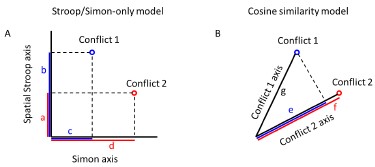
Therefore, we believe that the model comparisons between cosine similarity model and the Stroop/Simon-Only models were equitable. However, we acknowledge the reviewer’s and other reviewers’ concerns about the correlation between spatial Stroop and Simon conflicts, which reduces the space to one dimension (1d) and limits our ability to distinguish between the Stroop-only and Simon-only models, as well as between Stroop+Simon and cosine similarity models. While these distinctions are undoubtedly important for understanding the geometry of the cognitive space, we recognize that they go beyond the major objective of this study, that is, to differentiate the cosine similarity model from domain-general/specific models. Therefore, we have chosen to exclude the Stroop-only, Simon-only and Stroop+Simon models in our revised manuscript.
Something that raised additional concerns are the RSMs in the key region of interest (Fig S5). The pure stroop task appears to be represented very differently from all of the conditions that include simon conflict.
Together, I think these limitations reflect the structure of the task and research goals, not the statistical approach (which has been meaningfully improved).
Response: We appreciate the reviewer for pointing this out. It is essential to clarify that our conclusions were based on the significant similarity modulation effect identified in our statistical analysis using the cosine similarity model, where we did not distinguish between the within-Stroop condition and the other four within-conflict conditions (Fig. 7A, now Fig. 8A). This means that the representation of conflict type was not biased by the seemingly disparities in the values shown here. Moreover, to specifically test the differences between the within-Stroop condition and the other within-conflict conditions, we conducted a mixed-effect model analysis only including trial pairs from the same conflict type. In this analysis, the primary predictor was the cross-condition difference (0 for within-Stroop condition and 1 for other within-conflict conditions). The results showed no significant cross-condition difference in either the incongruent (t = 1.22, p = .23) or the congruent (t = 1.06, p = .29) trials. Thus, we believe the evidence for different similarities is inconclusive in our data and decided not to interpret this numerical difference. We have added this note in the revised figure caption for Figure S5.
Author response image 2.
Fig. S5. The stronger conflict type similarity effect in incongruent versus congruent conditions. (A) Summary representational similarity matrices for the right 8C region in incongruent (left) and congruent (right) conditions, respectively. Each cell represents the averaged Pearson correlation of cells with the same conflict type and congruency in the 1400×1400 matrix. Note that the seemingly disparities in the values of Stroop and other within-conflict cells (i.e., the diagonal) did not reach significance for either incongruent (t = 1.22, p = .23) or congruent (t = 1.06, p = .29) trials. (2) Scatter plot showing the averaged neural similarity (Pearson correlation) as a function of conflict type similarity in both conditions. The values in both A and B are calculated from raw Pearson correlation values, in contrast to the z-scored values in Fig. 4D.
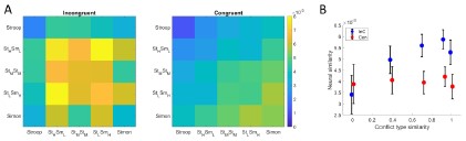
Minor:
- In the analysis of similarity_orientation, the df is very large (~14000). Here, and throughout, the df should be reflective of the population of subjects (ie be less than the sample size).
Response: The large degrees of freedom (df) in our analysis stem from the fact that we utilized a mixed-effect linear model, incorporating all data points (a total of 400×35=14000). In mixed-effect models, the df is determined by subtracting the number of fixed effects (in our case, 7) from the total number of observations. Notably, we are in line with the literature that have reported the df in this manner (e.g., Iravani et al., 2021; Schmidt & Weissman, 2015; Natraj et al., 2022).
Reference:
Iravani B, Schaefer M, Wilson DA, Arshamian A, Lundström JN. The human olfactory bulb processes odor valence representation and cues motor avoidance behavior. Proc Natl Acad Sci U S A. 2021 Oct 19;118(42):e2101209118. https://doi.org/10.1073/pnas.2101209118.
Schmidt, J.R., Weissman, D.H. Congruency sequence effects and previous response times: conflict adaptation or temporal learning?. Psychological Research 80, 590–607 (2016). https://doi.org/10.1007/s00426-015-0681-x.
Natraj, N., Silversmith, D. B., Chang, E. F., & Ganguly, K. (2022). Compartmentalized dynamics within a common multi-area mesoscale manifold represent a repertoire of human hand movements. Neuron, 110(1), 154-174. https://doi.org/10.1016/j.neuron.2021.10.002.
- it would improve the readability if there was more didactic justification for why analyses are done a certain way (eg justifying the jaccard metric). This will help less technically-savvy readers.
Response: We appreciate the reviewer’s suggestion. However, considering the Stroop/Simon-only models in our design may not be a valid approach for distinguishing the contributions of the Stroop/Simon components, we have decided not to include the Jaccard metrics in our revised manuscript.
Besides, to improve the readability, we have moved Figure S4 to the main text (labeled as Figure 7), and added the domain-general/domain-specific schematics in Figure 8.
Author response image 3.
Figure 8. Schematic of key RSMs. (A) and (B) show the orthogonality between conflict similarity and orientation RSMs. The within-subject RSMs (e.g., Group1-Group1) for conflict similarity and orientation are all the same, but the cross-group correlations (e.g., Group2-Group1) are different. Therefore, we can separate the contribution of these two effects when including them as different regressors in the same linear regression model. (C) and (D) show the two alternative models. Like the cosine model (A), within-group trial pairs resemble between-group trial pairs in these two models. The domain-specific model is an identity matrix. The domain-general model is estimated from the absolute difference of behavioral congruency effect, but scaled to 0(lowest similarity)-1(highest similarity) to aid comparison. The plotted matrices here include only one subject each from Group 1 and Group 2. Numbers 1-5 indicate the conflict type conditions, for spatial Stroop, StHSmL, StMSmM, StLSmH, and Simon, respectively. The thin lines separate four different sub-conditions, i.e., target arrow (up, down) × congruency (incongruent, congruent), within each conflict type.
Reviewer #2:
This study examines the construct of "cognitive spaces" as they relate to neural coding schemes present in response conflict tasks. The authors use a novel experimental design in which different types of response conflict (spatial Stroop, Simon) are parametrically manipulated. These conflict types are hypothesized to be encoded jointly, within an abstract "cognitive space", in which distances between task conditions depend only on the similarity of conflict types (i.e., where conditions with similar relative proportions of spatial-Stroop versus Simon conflicts are represented with similar activity patterns). Authors contrast such a representational scheme for conflict with several other conceptually distinct schemes, including a domain-general, domain-specific, and two task-specific schemes. The authors conduct a behavioral and fMRI study to test which of these coding schemes is used by prefrontal cortex. Replicating the authors' prior work, this study demonstrates that sequential behavioral adjustments (the congruency sequence effect) are modulated as a function of the similarity between conflict types. In fMRI data, univariate analyses identified activation in left prefrontal and dorsomedial frontal cortex that was modulated by the amount of Stroop or Simon conflict present, and representational similarity analyses (RSA) that identified coding of conflict similarity, as predicted under the cognitive space model, in right lateral prefrontal cortex.
This study tackles an important question regarding how distinct types of conflict might be encoded in the brain within a computationally efficient representational format. The ideas postulated by the authors are interesting ones and the statistical methods are generally rigorous.
Response: We would like to express our sincere appreciation for the reviewer’s positive evaluation of our manuscript and the constructive comments and suggestions. In response to your suggestions and concerns, we excluded the StroopOnly, SimonOnly and Stroop+Simon models, and added the schematic of domain-general/specific model RSMs. We have provided detailed responses to your comments below.
The evidence supporting the authors claims, however, is limited by confounds in the experimental design and by lack of clarity in reporting the testing of alternative hypotheses within the method and results.
- Model comparison
The authors commendably performed a model comparison within their study, in which they formalized alternative hypotheses to their cognitive space hypothesis. We greatly appreciate the motivation for this idea and think that it strengthened the manuscript. Nevertheless, some details of this model comparison were difficult for us to understand, which in turn has limited our understanding of the strength of the findings.
The text indicates the domain-general model was computed by taking the difference in congruency effects per conflict condition. Does this refer to the "absolute difference" between congruency effects? In the rest of this review, we assume that the absolute difference was indeed used, as using a signed difference would not make sense in this setting. Nevertheless, it may help readers to add this information to the text.
Response: We apologize for any confusion. The “difference” here indeed refers to the “absolute difference” between congruency effects. We have now clarified this by adding the word “absolute” accordingly.
"Therefore, we defined the domain-general matrix as the absolute difference in their congruency effects indexed by the group-averaged RT in Experiment 2."
Regarding the Stroop-Only and Simon-Only models, the motivation for using the Jaccard metric was unclear. From our reading, it seems that all of the other models --- the cognitive space model, the domain-general model, and the domain-specific model --- effectively use a Euclidean distance metric. (Although the cognitive space model is parameterized with cosine similarities, these similarity values are proportional to Euclidean distances because the points all lie on a circle. And, although the domain-general model is parameterized with absolute differences, the absolute difference is equivalent to Euclidean distance in 1D.) Given these considerations, the use of Jaccard seems to differ from the other models, in terms of parameterization, and thus potentially also in terms of underlying assumptions. Could authors help us understand why this distance metric was used instead of Euclidean distance? Additionally, if Jaccard must be used because this metric seems to be non-standard in the use of RSA, it would likely be helpful for many readers to give a little more explanation about how it was calculated.
Response: We believe that the Jaccard similarity measure is consistent with the Cosine similarity measure. The Jaccard similarity is calculated as the intersection divided by the union. To define the similarity of two conflicts in the Stroop-only and Simon-only models, we first project them onto the vertical or horizontal axes, respectively (as shown in Author response image 1A). The Jaccard similarity in our design is equivalent to the cosine similarity because the denominator in the Jaccard similarity is identical to the denominator in the cosine similarity (both are the radius of the circle, Author response image 1B).
However, it is important to note that a cosine similarity cannot be defined when conflicts are projected onto spatial Stroop or Simon axis simultaneously. Therefore, we used the Jaccard similarity in the previous version of our manuscript.
Author response image 4.
Definition of Jaccard similarity. A) Two conflicts (1 and 2) are projected onto the spatial Stroop/Simon axis in the Stroop/Simon-only model, respectively. The Jaccard similarity for Stroop-only and Simon-only model are and respectively. Letters a-d are the projected vectors from the two conflicts to the two axes. Blue and red colors indicate the conflict conditions. Shorter vectors are the intersection and longer vectors are the union. B) According to the cosine similarity model, the similarity is defined as , where e is the projected vector from conflict 1 to conflict 2, and g is the vector of conflict 1. The Jaccard similarity for this case is defined by , where f is the projector vector from conflict 2 to itself. Because f = g in our design, the Jaccard similarity is equivalent to the cosine similarity.
However, we agree with the reviewer’s and other reviewers’ concern that the correlation between spatial Stroop and Simon conflicts makes it less likely to distinguish the Stroop+Simon from cosine similarity models. While distinguishing them is essential to understand the detailed geometry of the cognitive space, it is beyond our major purpose, that is, to distinguish the cosine similarity model with the domain-general/specific models. Therefore, we have chosen to exclude the Stroop-only, Simon-only and Stroop+Simon models from our revised manuscript.
When considering parameterizing the Stroop-Only and Simon-Only models with Euclidean distances, one concern we had is that the joint inclusion of these models might render the cognitive space model unidentifiable due to collinearity (i.e., the sum of the Stroop-Only and Simon-Only models could be collinear with the cognitive space model). Could the authors determine whether this is the case? This issue seems to be important, as the presence of such collinearity would suggest to us that the design is incapable of discriminating those hypotheses as parameterized.
Response: We acknowledge that our design does not allow for a complete differentiation between the parallel encoding (StroopOnly+SimonOnly) model and the cognitive space model, given their high correlation (r = 0.85). However, it is important to note that the StroopOnly+SimonOnly model introduces more free parameters, making the model fitting poorer than the cognitive space model.
Additionally, the cognitive space model also shows high correlations with the StroopOnly and SimonOnly models (both rs = 0.66). It is crucial to emphasize that our study’s primary goal does not involve testing the parallel encoding hypothesis (through the StroopOnly+SimonOnly model). As a result, we have chosen to remove the model comparison results with the StroopOnly, SimonOnly and StroopOnly+SimonOnly models. Instead, the cognitive space model shows lower correlation with the purely domain-general (r = −0.16) and domain-specific (r = 0.46) models.
- Issue of uniquely identifying conflict coding
We certainly appreciate the efforts that authors have taken to address potential confounders for encoding of conflict in their original submission. We broach this question not because we wish authors to conduct additional control analyses, but because this issue seems to be central to the thesis of the manuscript and we would value reading the authors' thoughts on this issue in the discussion.
To summarize our concerns, conflict seems to be a difficult variable to isolate within aggregate neural activity, at least relative to other variables typically studied in cognitive control, such as task-set or rule coding. This is because it seems reasonable to expect that many more nuisance factors covary with conflict -- such as univariate activation, level of cortical recruitment, performance measures, arousal --- than in comparison with, for example, a well-designed rule manipulation. Controlling for some of these factors post-hoc through regression is commendable (as authors have done here), but such a method will likely be incomplete and can provide no guarantees on the false positive rate.
Relatedly, the neural correlates of conflict coding in fMRI and other aggregate measures of neural activity are likely of heterogeneous provenance, potentially including rate coding (Fu et al., 2022), temporal coding (Smith et al., 2019), modulation of coding of other more concrete variables (Ebitz et al., 2020, 10.1101/2020.03.14.991745; see also discussion and reviews of Tang et al., 2016, 10.7554/eLife.12352), or neuromodulatory effects (e.g., Aston-Jones & Cohen, 2005). Some of these origins would seem to be consistent with "explicit" coding of conflict (conflict as a representation), but others would seem to be more consistent with epiphenomenal coding of conflict (i.e., conflict as an emergent process). Again, these concerns could apply to many variables as measured via fMRI, but at the same time, they seem to be more pernicious in the case of conflict. So, if authors consider these issues to be germane, perhaps they could explicitly state in the discussion whether adopting their cognitive space perspective implies a particular stance on these issues, how they interpret their results with respect to these issues, and if relevant, qualify their conclusions with uncertainty on these issues.
Response: We appreciate the reviewer’s insightful comments regarding the representation and process of conflict.
First, we agree that the conflict is not simply a pure feature like a stimulus but often arises from the interaction (e.g., dimension overlap) between two or more aspects. For example, in the manual Stroop, conflict emerges from the inconsistent semantic information between color naming and word reading. Similarly, other higher-order cognitive processes such as task-set also underlie the relationship between concrete aspects. For instance, in a face/house categorization task, the taskset is the association between face/house and the responses. When studying these higher-order processes, it is often impossible to completely isolate them from bottomup features. Therefore, methods like the representational similarity analysis and regression models are among the limited tools available to attempt to dissociate these concrete factors from conflict representation. While not perfect, this approach has been suggested and utilized in practice (Freund et al., 2021).
Second, we agree that conflict can be both a representation and an emerging process. These two perspectives are not necessarily contradictory. According to David Marr’s influential three-level theory (Marr, 1982), representation is the algorithm of the process to achieve a goal based on the input. Therefore, a representation can refer to not only a static stimulus (e.g., the visual representation of an image), but also a dynamic process. Building on this perspective, we posit that the representation of cognitive control consists of an array of dynamic representations embedded within the overall process. A similar idea has been proposed that the abstract task profiles can be progressively constructed as a representation in our brain (Kikumoto & Mayr, 2020).
We have incorporated this discussion into the manuscript:
"Recently an interesting debate has arisen concerning whether cognitive control should be considered as a process or a representation (Freund, Etzel, et al., 2021). Traditionally, cognitive control has been predominantly viewed as a process. However, the study of its representation has gained more and more attention. While it may not be as straightforward as the visual representation (e.g., creating a mental image from a real image in the visual area), cognitive control can have its own form of representation. An influential theory, Marr’s (1982) three-level model proposed that representation serves as the algorithm of the process to achieve a goal based on the input. In other words, representation can encompass a dynamic process rather than being limited to static stimuli. Building on this perspective, we posit that the representation of cognitive control consists of an array of dynamic representations embedded within the overall process. A similar idea has been proposed that the representation of task profiles can be progressively constructed with time in the brain (Kikumoto & Mayr, 2020)."
Reference:
Freund, M. C., Etzel, J. A., & Braver, T. S. (2021). Neural Coding of Cognitive Control: The Representational Similarity Analysis Approach. Trends in Cognitive Sciences, 25(7), 622-638. https://doi.org/10.1016/j.tics.2021.03.011
Marr, D. C. (1982). Vision: A computational investigation into human representation and information processing. New York: W.H. Freeman.
Kikumoto A, Mayr U. (2020). Conjunctive representations that integrate stimuli, responses, and rules are critical for action selection. Proceedings of the National Academy of Sciences, 117(19):10603-10608. https://doi.org/10.1073/pnas.1922166117.
- Interpretation of measured geometry in 8C
We appreciate the inclusion of the measured similarity matrices of area 8C, the key area the results focus on, to the supplemental, as this allows for a relatively model-agnostic look at a portion of the data. Interestingly, the measured similarity matrix seems to mismatch the cognitive space model in a potentially substantive way. Although the model predicts that the "pure" Stroop and Simon conditions will have maximal self-similarity (i.e., the Stroop-Stroop and Simon-Simon cells on the diagonal), these correlations actually seem to be the lowest, by what appears to be a substantial margin (particularly the Stroop-Stroop similarities). What should readers make of this apparent mismatch? Perhaps authors could offer their interpretation on how this mismatch could fit with their conclusions.
Response: We appreciate the reviewer for bringing this to our attention. It is essential to clarify that our conclusions were based on the significant similarity modulation effect observed in our statistical analysis using the cosine similarity model, where we did not distinguish between the within-Stroop condition and the other four withinconflict conditions (Fig. 7A). This means that the representation of conflict type was not biased by the seemingly disparities in the values shown here. Moreover, to specifically address the potential differences between the within-Stroop condition and the other within-conflict conditions, we conducted a mixed-effect model. In this analysis, the primary predictor was the cross-condition difference (0 for within-Stroop condition and 1 for other within-conflict conditions). The results showed no significant cross-condition difference in either the incongruent trials (t = 1.22, p = .23) or the congruent (t = 1.06, p = .29) trials. Thus, we believe the evidence for different similarities is inconclusive in our data and decided not to interpret this numerical difference.
We have added this note in the revised figure caption for Figure S5.
Author response image 5.
Fig. S5. The stronger conflict type similarity effect in incongruent versus congruent conditions. (A) Summary representational similarity matrices for the right 8C region in incongruent (left) and congruent (right) conditions, respectively. Each cell represents the averaged Pearson correlation of cells with the same conflict type and congruency in the 1400×1400 matrix. Note that the seemingly disparities in the values of Stroop and other within-conflict cells (i.e., the diagonal) did not reach significance for either incongruent (t = 1.22, p = .23) or congruent (t = 1.06, p = .29) trials. (2) Scatter plot showing the averaged neural similarity (Pearson correlation) as a function of conflict type similarity in both conditions. The values in both A and B are calculated from raw Pearson correlation values, in contrast to the z-scored values in Fig. 4D.
- It would likely improve clarity if all of the competing models were displayed as summarized RSA matrices in a single figure, similar to (or perhaps combined with) Figure 7.
Response: We appreciate the reviewer’s suggestion. We now have incorporated the domain-general and domain-specific models into the Figure 7 (now Figure 8).
Author response image 6.
Figure 8. Schematic of key RSMs. (A) and (B) show the orthogonality between conflict similarity and orientation RSMs. The within-subject RSMs (e.g., Group1-Group1) for conflict similarity and orientation are all the same, but the cross-group correlations (e.g., Group2-Group1) are different. Therefore, we can separate the contribution of these two effects when including them as different regressors in the same linear regression model. (C) and (D) show the two alternative models. Like the cosine model (A), within-group trial pairs resemble between-group trial pairs in these two models. The domain-specific model is an identity matrix. The domain-general model is estimated from the absolute difference of behavioral congruency effect, but scaled to 0(lowest similarity)-1(highest similarity) to aid comparison. The plotted matrices here include only one subject each from Group 1 and Group 2. Numbers 1-5 indicate the conflict type conditions, for spatial Stroop, StHSmL, StMSmM, StLSmH, and Simon, respectively. The thin lines separate four different sub-conditions, i.e., target arrow (up, down) × congruency (incongruent, congruent), within each conflict type.
- Because this model comparison is key to the main inferences in the study, it might also be helpful for most readers to move all of these RSA model matrices to the main text, instead of in the supplemental.
Response: We thank the reviewer for this suggestion. We have moved the Fig. S4 to the main text, labeled as the new Figure 7.
- It may be worthwhile to check how robust the observed brain-behavior association (Fig 4C) is to the exclusion of the two datapoints with the lowest neural representation strength measure, as these points look like they have high leverage.
Response: We calculated the Pearson correlation after excluding the two points and found it does not affect the results too much, with the r = 0.50, p = .003 (compared to the original r = 0.52, p = .001).
Additionally, we found the two axes were mistakenly shifted in Fig 4C. Therefore, we corrected this error in the revised manuscript. The correlation results would not be influenced.
Author response image 7.
Fig. 4. The conflict type effect. (A) Brain regions surviving the Bonferroni correction (p < 0.0001) across the regions (criterion 1). Labeled regions are those meeting the criterion 2. (B) Different encoding of conflict type in the incongruent with congruent conditions. * Bonferroni corrected p < .05. (C) The brain-behavior correlation of the right 8C (criterion 3). The x-axis shows the beta coefficient of the conflict type effect from the RSA, and the y-axis shows the beta coefficient obtained from the behavioral linear model using the conflict similarity to predict the CSE in Experiment 2. (D) Illustration of the different encoding strength of conflict type similarity in incongruent versus congruent conditions of right 8C. The y-axis is derived from the z-scored Pearson correlation coefficient, consistent with the RSA methodology. See Fig. S4B for a plot with the raw Pearson correlation measurement. l = left; r = right.
Reviewer #3:
Yang and colleagues investigated whether information on two task-irrelevant features that induce response conflict is represented in a common cognitive space. To test this, the authors used a task that combines the spatial Stroop conflict and the Simon effect. This task reliably produces a beautiful graded congruency sequence effect (CSE), where the cost of congruency is reduced after incongruent trials. The authors measured fMRI to identify brain regions that represent the graded similarity of conflict types, the congruency of responses, and the visual features that induce conflicts. They applied univariate, multivariate, and connectivity analyses to fMRI data to identify brain regions that represent the graded similarity of conflict types, the congruency of responses, and the visual features that induce conflicts. They further directly assessed the dimensionality of represented conflict space.
The authors identified the right dlPFC (right 8C), which shows 1) stronger encoding of graded similarity of conflicts in incongruent trials and 2) a positive correlation between the strength of conflict similarity type and the CSE on behavior. The dlPFC has been shown to be important for cognitive control tasks. As the dlPFC did not show a univariate parametric modulation based on the higher or lower component of one type of conflict (e.g., having more spatial Stroop conflict or less Simon conflict), it implies that dissimilarity of conflicts is represented by a linear increase or decrease of neural responses. Therefore, the similarity of conflict is represented in multivariate neural responses that combine two sources of conflict.
The strength of the current approach lies in the clear effect of parametric modulation of conflict similarity across different conflict types. The authors employed a clever cross-subject RSA that counterbalanced and isolated the targeted effect of conflict similarity, decorrelating orientation similarity of stimulus positions that would otherwise be correlated with conflict similarity. A pattern of neural response seems to exist that maps different types of conflict, where each type is defined by the parametric gradation of the yoked spatial Stroop conflict and the Simon conflict on a similarity scale. The similarity of patterns increases in incongruent trials and is correlated with CSE modulation of behavior.
The main significance of the paper lies in the evidence supporting the use of an organized "cognitive space" to represent conflict information as a general control strategy. The authors thoroughly test this idea using multiple approaches and provide convincing support for their findings. However, the universality of this cognitive strategy remains an open question.
(Public Reviews) Taken together, this study presents an exciting possibility that information requiring high levels of cognitive control could be flexibly mapped into cognitive map-like representations that both benefit and bias our behavior. Further characterization of the representational geometry and generalization of the current results look promising ways to understand representations for cognitive control.
Response: We would like to thank the reviewer for the positive evaluation of our manuscript and for providing constructive comments. In response to your suggestions, we have acknowledged the potential limitation of the design and the cross-subject RSA approach, and incorporated the open questions to the discussions. Please find our detailed responses below.
The task presented in the study involved two sources of conflict information through a single salient visual input, which might have encouraged the utilization of a common space.
Response: We agree that the unified visual input in our design may have facilitated the utilization of a common space. However, we believe the stimuli are not necessarily unified in the construction of the common space. To further test the potential interaction between the concrete stimulus setting and the cognitive space representation, it is necessary to use varied stimuli in future research. We have left this as an open question in the discussion:
Can we effectively map any sources of conflict with completely different stimuli into a single space?
The similarity space was analyzed at the level of between-individuals (i.e., crosssubject RSA) to mitigate potential confounds in the design, such as congruency and the orientation of stimulus positions. This approach makes it challenging to establish a direct link between the quality of conflict space representation and the patterns of behavioral adaptations within individuals.
Response: By setting the variables as random effects at the subject level, we have extracted the individual effects that incorporate both the group-level fixed effects and individual-level random effects. We believe this approach yields results that are as reliable, if not more, than effects calculated from individual data only. First, the mixed effect linear (LME) model has included all the individual data, forming the basis for establishing random effects. Therefore, the individual effects derived from this approach inherently reflect the individual-specific effects. To support this notion, we have included a simulation script (accessible in the online file “simulation_LME.mlx” at https://osf.io/rcq8w) to demonstrate the strong consistency between the two approaches (see Author response image 8). In this simulation, we generated random data (Y) for 35 subjects, each containing 20 repeated measurements across 5 conditions. To streamline the simulation, we only included one predictor (X), which was treated as both fixed and random effects at the subject level. We applied two methods to calculate the individual beta coefficient. The first involved extracting individual beta coefficients from the LME model by summing the fixed effect with the subject-specific random effect. The second method was entailed conducting a regression analysis using data from each subject to obtain the slope. We tested their consistency by calculating the Pearson correlation between the derived beta coefficients. This simulation was repeated 100 times.
Author response image 8.
The consistent individual beta coefficients between the mixed effect model and the individual regression analysis. A) The distribution of Pearson correlation between the two methods for 100 times. B) An example from the simulation showing the highly correlated results from the two methods. Each data point indicates a subject (n=35).
Second, the potential difference between the two methods lies in that the LME model have also taken the group-level variance into account, such as the dissociable variances of the conflict similarity and orientation across subject groups. This enabled us to extract relatively cleaner conflict similarity effects for each subject, which we believe can be better linked to the individual behavioral adaptations. Moreover, we have extracted the behavioral adaptations scores (i.e., the similarity modulation effect on CSE) using a similar LME approach. Conducting behavioral analysis solely using individual data would have been less reliable, given the limited sample size of individual data (~32 points per subject). This also motivated us to maintain consistency by extracting individual neural effects using LME models.
Furthermore, it remains unclear at which cognitive stages during response selection such a unified space is recruited. Can we effectively map any sources of conflict into a single scale? Is this unified space adaptively adjusted within the same brain region? Additionally, does the amount of conflict solely define the dimensions of this unified space across many conflict-inducing tasks? These questions remain open for future studies to address.
Response: We appreciate the reviewer’s constructive open questions. We respond to each of them based on our current understanding.
1) It remains unclear at which cognitive stages during response selection such a unified space is recruited.
We anticipate that the cognitive space is recruited to guide the transference of behavioral CSE at two critical stages. The first stage involves the evaluation of control demands, where the representational distance/similarity between previous and current trials influences the adjustment of cognitive control. The second stage pertains to is control execution, where the switch from one control state to another follows a path within the cognitive space. It is worth noting that future studies aiming to address this question may benefit from methodologies with higher temporal resolutions, such as EEG and MEG, to provide more precise insights into the temporal dynamics of the process of cognitive space recruitment.
2) Can we effectively map any sources of conflict into a single scale?
It is possible that various sources of conflict can be mapped onto the same space based on their similarity, even if finding such an operational defined similarity may be challenging. However, our results may offer an approach to infer the similarity between two conflicts. One way is to examine their congruency sequence effect (CSE), with a stronger CSE suggesting greater similarity. The other way is to test their representational similarity within the dorsolateral prefrontal cortex.
3) Is this unified space adaptively adjusted within the same brain region? We do not have an answer to this question. We showed that the cognitive space does not change with time (Note. S3). What have adjusted is the control demand to resolve the quickly changing conflict conditions from trial to trial. Though, it is an interesting question whether the cognitive space may be altered, for example, when the mental state changes significantly. And if yes, we can further test whether the change of cognitive space is also within the right dlPFC.
4) Additionally, does the amount of conflict solely define the dimensions of this unified space across many conflict-inducing tasks?
Our understanding of this comment is that the amount of conflict refers to the number of conflict sources. Based on our current finding, the dimensions of the space are indeed defined by how many different conflict sources are included. However, this would require the different conflict sources are orthogonal. If some sources share some aspects, the cognitive space may collapse to a lower dimension. We have incorporated the first question into the discussion:
Moreover, we anticipate that the representation of cognitive space is most prominently involved at two critical stages to guide the transference of behavioral CSE. The first stage involves the evaluation of control demands, where the representational distance/similarity between previous and current trials influences the adjustment of cognitive control. The second stage pertains to control execution, where the switch from one control state to another follows a path within the cognitive space. However, we were unable to fully distinguish between these two stages due to the low temporal resolution of fMRI signals in our study. Future research seeking to delve deeper into this question may benefit from methodologies with higher temporal resolutions, such as EEG and MEG.
We have included the other questions into the manuscript as open questions, calling for future research.
Several interesting questions remains to be answered. For example, is the dimension of the unified space across conflict-inducing tasks solely determined by the number of conflict sources? Can we effectively map any sources of conflict with completely different stimuli into a single space? Is the cognitive space geometry modulated by the mental state? If yes, what brain regions mediate the change of cognitive space?
Minor comments:
- The original comment about out-of-sample predictions to examine the continuity of the space was a suggestion for testing neural representations, not behavior (I apologize for the lack of clarity). Given the low dimensionality of the conflict space shown by the participation ratio, we expect that linear separability exists only among specific combinations of conditions. For example, the pair of conflicts 1 and 5 together is not linearly separable from conflicts 2 and 3. But combined with other results, this is already implied.
Response: We apologize for the misunderstanding. In fact, performing a prediction analysis using the extensive RSM in our study does presents certain challenges, primarily due to its substantial size (1400x1400) and the intricate nature of the mixed-effect linear model. In our efforts to simplify the prediction process by excluding random effects, we did observe a correlation between the predicted and original values, albeit a relatively small Pearson correlation coefficient of r = 0.024, p < .001. This small correlation can be attributed to two key factors. First, the exclusion of data points impacts not only the conflict similarity regressor but also other regressors within the model, thereby diminishing the predictive power. Secondly, the large amount of data points in the model heightens the risk of overfitting, subsequently reducing the model’s capacity for generalization and increasing the likelihood of unreliable predictions. Given these potential problems, we have opted not to include this prediction in the revised manuscript.
Author response:
The following is the authors’ response to the previous reviews
Editor's note:
Thank you for taking time and efforts to improve this study. After re-review, two reviewers have a consensus that the connections the fatty acids and sperm motility is still ambiguous. Thus, I recommend to further tone down this conclusion consistently in the title and the text pointed out by reviewers before making a final version of record.
We sincerely appreciate the considerable time and effort you and the reviewers devoted to evaluating our manuscript. We have revised the title and text to express the relationship between fatty acids and sperm motility more consistently and toned down. With these revisions, we would like to proceed with publishing the manuscript as the Version of Record (VoR). Thank you very much for your guidance in improving our study.
Public Reviews:
Reviewer #1 (Public review):
Summary:
In this revised report, Yamanaka and colleagues investigate a proposed mechanism by which testosterone modulates seminal plasma metabolites in mice. Based on limited evidence in previous versions of the report, the authors softened the claim that oleic acid derived from seminal vesicle epithelium strongly affects linear progressive motility in isolated cauda epididymal sperm in vitro. Though the report still contains somewhat ambiguous references to the strength of the relationship between fatty acids and sperm motility.
Strengths:
Often, reported epidydimal sperm from mice have lower percent progressive motility compared with sperm retrieved from the uterus or by comparison with human ejaculated sperm. The findings in this report may improve in vitro conditions to overcome this problem, as well as add important physiological context to the role of reproductive tract glandular secretions in modulating sperm behaviors. The strongest observations are related to the sensitivity of seminal vesicle epithelial cells to testosterone. The revisions include the addition of methodological detail, modified language to reflect the nuance of some of the measurements, as well as re-performed experiments with more appropriate control groups. The findings are likely to be of general interest to the field by providing context for follow-on studies regarding the relationship between fatty acid beta oxidation and sperm motility pattern.
Weaknesses:
The connection between media fatty acids and sperm motility pattern remains inconclusive.
We would like to express our sincere gratitude to the judges for their cooperation in reviewing the manuscript and for your helpful comments, which were instrumental in improving manuscript.
Reviewer #2 (Public review):
Using a combination of in vivo studies with testosterone-inhibited and aged mice with lower testosterone levels as well as isolated mouse and human seminal vesicle epithelial cells the authors show that testosterone induces an increase in glucose uptake. They find that testosterone induces a difference in gene expression with a focus on metabolic enzymes. Specifically, they identify increased expression of enzymes regulating cholesterol and fatty acid synthesis, leading to increased production of 18:1 oleic acid. The revised version strengthens the role of ACLY as the main regulator of seminal vesicle epithelial cell metabolic programming. The authors propose that fatty acids are secreted by seminal vesicle epithelial cells and are taken up by sperm, positively affecting sperm function. A lipid mixture mimicking the lipids secreted by seminal vesicle epithelial cells, however, only has a small and mostly non-significant effect on sperm motility, suggesting the authors were not apply to pinpoint the seminal vesicle fluid component that positively affects sperm function.
We greatly appreciate the reviewer’s thoughtful comments and time spent reviewing this manuscript. The relationship between lipids such as fatty acids and sperm motility remains unclear in the current dataset. Therefore, before finalizing the manuscript, we revised the title and text, as suggested by the reviewers, to express this conclusion more cautiously and consistently.
Recommendations for the authors:
Reviewer #1 (Recommendations for the authors):
Some additional comments are provided below to aid the authors in improving the quality of the work:
Major Comments:
(1) In the newly added supplemental figure 5, the authors note that the percentage data were arcisine transformed prior to statistical analysis without providing any other justification. This seems strange, especially for such a small sample size. It seems more appropriate for the authors to use a nonparametric test. Forcing symmetry without knowing what the shape of the true distribution is makes the ANOVA hard to interpret. Additionally, why use pairwise comparisons rather than comparing each group to the control (LM 0%). Also, note that the graphs are not individually labeled to distinguish them in the legend (A, B, C, etc.). Ultimately, the treatment differences don't seem that meaningful, even if the authors were able to observe statistical significance with the somewhat over-manipulated method of analysis.
Ultimately, the conclusion of this experiment (Supplemental figure 5) remains unchanged, but we agree that the relationship between fatty acids and sperm motility remains unclear. Therefore, before finalizing the manuscript, we revised the title and text as pointed out by the reviewers to express this conclusion more cautiously and consistently throughout the manuscript.
Arcsin transform is commonly used for percentage data [Zar, J.H. 2010. Biostatistical analysis., McDonald, J.H. 2014. Handbook of biological statistics.]. If the values are low or high, such as 0 to 30% or 70 to 100%, without arcsine transformation will result in a large deviation from the normality of the data. However, even if such a conversion is performed, it does not necessarily mean that the assumptions of normality and homogeneity of variance, which are prerequisites for parametric statistical analysis methods, are satisfied.
Given the small sample size and the possibility of non-normal data, we performed Shapiro–Wilk tests for each group (n = 6) and found no departure from normality (all p > 0.1). Q–Q plots and Levene’s test (p > 0.1) likewise supported the assumptions of ANOVA. Following the reviewer’s recommendation, we repeated the analysis with a Kruskal–Wallis test followed by Dunn’s post-hoc comparisons (Bonferroni corrected). Both approaches led to the same conclusions, with non-parametric p-values equal to or smaller than the parametric ones. In the revised manuscript we now report ANOVA as the primary analysis. The author response image includes effect sizes with 95 % confidence intervals, and provide the non-parametric results for transparency.
Author response image 1.
Results of reanalysis of supplementary Figure 5 using nonparametric tests and effect sizes with 95% confidence intervals. Upper part; Differences between groups were assessed by Kruskal–Wallis test, differences among values were analyzed by Dunn’s post-hoc comparisons (Bonferroni corrected) for multiple comparisons. Different letters represent significantly different groups. Lower part; The effect sizes with 95 % confidence intervals. For example, Cliff's Δ = -1 (95% CI ~ -0.6) in VSL's “LM 0 vs LM1” means that LM 1% values exceed LM 0 %values in all pairs.
(2) I appreciate that the authors toned down the interpretation of the effects of seminal plasma metabolites on sperm motility with a cautionary statement on Lines 397-405 and Line 259. However, they send mixed signals with the title of the report: "Testosterone-Induced Metabolic Changes in Seminal Vesicle Epithelial cells Alter Plasma Components to Enhance Sperm Motility", and on line 265 when the say "ACLY expression is upregulated by testosterone and is essential for the metabolic shift of seminal vesicle epithelial cells that mediates sperm linear motility".
The wording has been softened overall. The title has been changed to “Testosterone-Induced Metabolic Changes in Seminal Vesicle Epithelium Modify Seminal Plasma Components with Potential to Improve Sperm Motility” In the results (lines 265-266), we have stated that “ACLY expression is upregulated by testosterone and is essential for the metabolic shift that is associated with increased linear motility” without implying a causal relationship.
Minor Comments:
(1) Typo on line 31: "understanding the male fertility mechanisms and may perspective for the development of potential biomarkers of male fertility and advance in the treatment of male infertility."
We have made the following corrections. “These findings suggest that testosterone-dependent lipid remodeling may contribute to sperm straight-line motility, and further functional verification is required.”
(2) Line 193: the statement is confusing "Therefore, we analyzed mitochondrial metabolism using a flux analyzer, predicting that more glucose is metabolized, pyruvate is metabolized from phosphoenolpyruvic acid through glycolysis in response to testosterone, and is further metabolized in the mitochondria." For example, 'Metabolized through glycolysis' is an ambiguous way to describe the pyruvate kinase reaction. Additionally, phosphoenolpyruvate has three acid ionizable groups, two of which have pKa's well below physiological pH, so phosphoenolpyruvate is the correct intermediate rather than phosphoenolpyruvic acid. The authors make similar mistakes with other organic acids such as citric acid.
Rewritten as “We therefore examined cellular energy metabolism with a flux analyzer, anticipating that testosterone would elevate glycolytic flux, thereby producing more pyruvate from phosphoenolpyruvate. Because extracellular pyruvate levels simultaneously declined, we inferred that the cells had an increased pyruvate demand and, at that time, hypothesized that the excess pyruvate would enter the mitochondria to support enhanced oxidative metabolism.” (lines 193-198)
The organic acids are now referenced in their appropriate forms (e.g., citrate, phosphoenolpyruvate).
(3) Line: 271: "Acly" should be all capitalized to "ACLY". The report mixes capitalizing through out and could be more consistent.
We appreciate the reviewer’s attention to nomenclature and have standardized the manuscript accordingly. Proteins are written in Roman letters, all in capital letters. Mouse gene symbols: italics, first letter capitalize.
Reviewer #2 (Recommendations for the authors):
Major comments:
(1) 'Once capacitation is complete, sperm cannot maintain that state for a long time'. The publications cited by the author do not support that statement and this reviewer also does not agree. Lower fertilization efficiency from in vitro capacitated epidydimal sperm does not have to mean capacitation is reversed, it can simply mean in vitro capacitation conditions not accurately mimic capacitation in vivo.
We thank the reviewer for pointing this out and would like to clarify our position. Our statement does not suggest a "reversal" of active capacitation. Rather, it reflects the well-documented fact that capacitation is a transient process. Sperm that undergo capacitation too early cannot maintain that state for long enough to retain their ability to fertilize at the moment and location of fertilization in vivo.
(2) How do the authors explain the discrepancy between the results shown in Fig. S1E, the increase in sperm motility upon mixing of sperm with SVF and the results reported in Li et al 2025. Mentioning decapacitating factors without further explanation is insufficient.
We appreciate the reviewer's feedback pointing out the need for a clearer explanation.
Seminal plasma is inherently binary, containing both decapacitation factors that delay or inhibit capacitation and nutrient substrates that promote sperm motility.
In vivo, it is believed that the coating of sperm by decapacitation factors is removed by uterine fluid and albumin as it passes through the female reproductive tract [PMID: 22827391, PMID: 24274412]. In contrast, standard fertilization culture media lack a clearance pathway, so decapacitating factors are retained throughout the culture period. As a result, the cleavage rate after in vitro fertilization using sperm exposed to seminal vesicle fluid decreased dramatically.
Lipids, such as fatty acids, increased sperm motility without directly inducing markers of fertilization. These results suggest that the enhancement of motility by lipids is functionally distinct from the capacitation-inhibiting function of seminal plasma proteins. The data from this study are consistent with the biphasic model. Specifically, decapacitation factors temporarily stabilize the sperm membrane, preventing early capacitation. Meanwhile, lipids enhance sperm motility, enabling them to rapidly pass through the hostile uterine environment.
(3) This reviewer does not see the merit in including a lipid mixture motility experiment compared to using OA alone. The increase in motility is still small and far from comparable to the motility increase with seminal vesicle fluid. In this reviewer's opinion the experiment is still inconclusive and should not be highlighted in the manuscript title.
The wording has been softened overall. The title has been changed to “Testosterone-Induced Metabolic Changes in Seminal Vesicle Epithelium Modify Seminal Plasma Components with Potential to Improve Sperm Motility”. (Please see also Reviewer 1's main comment 1)
Minor comments:
(1) 'This change includes a large amplitude of flagella' does not make sense. Please correct.
The following corrections have been made. “This change is characterized by large-amplitude flagellar beating.” (lines 44-45)
Author response:
The following is the authors’ response to the previous reviews.
To the Senior Editor and the Reviewing Editor:
We sincerely appreciate the valuable comments provided by the reviewers, the reviewing editor, and the senior editor. Based on our last response and revision, we are confused by the two limitations noted in the eLife assessment.
(1) benchmarking against comparable methods is limited.
In our last revision, we added the comparison experiments with TNDM, as the reviewers requested. Additionally, it is crucial to emphasize that our evaluation of decoding capabilities of behaviorally relevant signals has been benchmarked against the performance of the ANN on raw signals, which, as Reviewer #1 previously noted, nearly represents the upper limit of performance. Consequently, we believe that our benchmarking methods are sufficiently strong.
(2) some observations may be a byproduct of their method, and may not constitute new scientific observations.
We believe that our experimental results are sufficient to demonstrate that our conclusions are not byproducts of d-VAE based on three reasons:
(1) The d-VAE, as a latent variable model, adheres to the population doctrine, which posits that latent variables are responsible for generating the activities of individual neurons. The goal of such models is to maximize the explanation of the raw signals. At the signal level, the only criterion we can rely on is neural reconstruction performance, in which we have achieved unparalleled results. Thus, it is inappropriate to focus on the mixing process during the model's inference stage while overlooking the crucial de-mixing process during the generation stage and dismissing the significance of our neural reconstruction results. For more details, please refer to the first point in our response to Q4 from Reviewer #4.
(2) The criterion that irrelevant signals should contain minimal information can effectively demonstrate that our conclusions are not by-products of d-VAE. Unfortunately, the reviewers seem to have overlooked this criterion. For more details, please refer to the third point in our response to Q4 from Reviewer #4
(3) Our synthetic experimental results also substantiate that our conclusions are not byproducts of d-VAE. However, it appears the reviewers did not give these results adequate consideration. For more details, please refer to the fourth point in our response to Q4 from Reviewer #4.
Furthermore, our work presents not just "a useful method" but a comprehensive framework. Our study proposes, for the first time, a framework for defining, extracting, and validating behaviorally relevant signals. In our current revision, to clearly distinguish between d-VAE and other methods, we have formalized the extraction of behaviorally relevant signals into a mathematical optimization problem. To our knowledge, current methods have not explicitly proposed extracting behaviorally relevant signals, nor have they identified and addressed the key challenges of extracting relevant signals. Similarly, existing research has not yet defined and validated behaviorally relevant signals. For more details, please refer to our response to Q1 from Reviewer #4.
Based on these considerations, we respectfully request that you reconsider the eLife assessment of our work. We greatly appreciate your time and attention to this matter.
The main revisions made to the manuscript are as follows:
(1) We have formalized the extraction of behaviorally relevant signals into a mathematical optimization problem, enabling a clearer distinction between d-VAE and other models.
(2) We have moderated the assertion about linear readout to highlight its conjectural nature and have broadened the discussion regarding this conclusion.
(3) We have elaborated on the model details of d-VAE and have removed the identifiability claim.
To Reviewer #1
Q1: “As reviewer 3 also points out, I would, however, caution to interpret this as evidence for linear read-out of the motor system - your model performs a non-linear transformation, and while this is indeed linearly decodable, the motor system would need to do something similar first to achieve the same. In fact to me it seems to show the opposite, that behaviour-related information may not be generally accessible to linear decoders (including to down-stream brain areas).”
Thank you for your comments. It's important to note that the conclusions we draw are speculative and not definitive. We use terms like "suggest" to reflect this uncertainty. To further emphasize the conjectural nature of our conclusions, we have deliberately moderated our tone.
The question of whether behaviorally-relevant signals can be accessed by linear decoders or downstream brain regions hinges on the debate over whether the brain employs a strategy of filtering before decoding. If the brain employs such a strategy, the brain can probably access these signals. In our opinion, it is likely that the brain utilizes this strategy.
Given the existence of behaviorally relevant signals, it is reasonable to assume that the brain has intrinsic mechanisms to differentiate between relevant and irrelevant signals. There is growing evidence suggesting that the brain utilizes various mechanisms, such as attention and specialized filtering, to suppress irrelevant signals and enhance relevant signals [1-3]. Therefore, it is plausible that the brain filters before decoding, thereby effectively accessing behaviorally relevant signals.
Thank you for your valuable feedback.
(1) Sreenivasan, Sameet, and Ila Fiete. "Grid cells generate an analog error-correcting code for singularly precise neural computation." Nature neuroscience 14.10 (2011): 1330-1337.
(2) Schneider, David M., Janani Sundararajan, and Richard Mooney. "A cortical filter that learns to suppress the acoustic consequences of movement." Nature 561.7723 (2018): 391-395.
(3) Nakajima, Miho, L. Ian Schmitt, and Michael M. Halassa. "Prefrontal cortex regulates sensory filtering through a basal ganglia-to-thalamus pathway." Neuron 103.3 (2019): 445-458.
Q2: “As in my initial review, I would also caution against making strong claims about identifiability although this work and TNDM seem to show that in practise such methods work quite well. CEBRA, in contrast, offers some theoretical guarantees, but it is not a generative model, so would not allow the type of analysis done in this paper. In your model there is a para,eter \alpha to balance between neural and behaviour reconstruction. This seems very similar to TNDM and has to be optimised - if this is correct, then there is manual intervention required to identify a good model.”
Thank you for your comments.
Considering your concerns about our identifiability claims and the fact that identifiability is not directly relevant to the core of our paper, we have removed content related to identifiability.
Firstly, our model is based on the pi-VAE, which also has theoretical guarantees. However, it is important to note that all such theoretical guarantees (including pi-VAE and CEBRA) are based on certain assumptions that cannot be validated as the true distribution of latent variables remains unknown.
Secondly, it is important to clarify that the identifiability of latent variables does not impact the conclusions of this paper, nor does this paper make specific conclusions about the model's latent variables. Identifiability means that distinct latent variables correspond to distinct observations. If multiple latent variables can generate the same observation, it becomes impossible to determine which one is correct given the observation, which leads to the issue of nonidentifiability. Notably, our analysis focuses on the generated signals, not the latent variables themselves, and thus the identifiability of these variables does not affect our findings.
Our approach, dedicated to extracting these signals, distinctly differs from methods such as TNDM, which focuses on extracting behaviorally relevant latent dynamics. To clearly set apart d-VAE from other models, we have framed the extraction of behaviorally relevant signals as the following mathematical optimization problem:
where 𝑥# denotes generated behaviorally-relevant signals, 𝑥 denotes raw noisy signals, 𝐸(⋅,⋅) demotes reconstruction loss, and 𝑅(⋅) denotes regularization loss. It is important to note that while both d-VAE and TNDM employ reconstruction loss, relying solely on this term is insufficient for determining the optimal degree of similarity between the generated and raw noisy signals. The key to accurately extracting behaviorally relevant signals lies in leveraging prior knowledge about these signals to determine the optimal similarity degree, encapsulated by 𝑅(𝒙𝒓). Other studies have not explicitly proposed extracting behaviorally-relevant signals, nor have they identified and addressed the key challenges involved in extracting relevant signals. Consequently, our approach is distinct from other methods.
Thank you for your valuable feedback.
Q3: “Somewhat related, I also found that the now comprehensive comparison with related models shows that the using decoding performance (R2) as a metric for model comparison may be problematic: the R2 values reported in Figure 2 (e.g. the MC_RTT dataset) should be compared to the values reported in the neural latent benchmark, which represent well-tuned models (e.g. AutoLFADS). The numbers (difficult to see, a table with numbers in the appendix would be useful, see: https://eval.ai/web/challenges/challenge-page/1256/leaderboard) seem lower than what can be obtained with models without latent space disentanglement. While this does not necessarily invalidate the conclusions drawn here, it shows that decoding performance can depend on a variety of model choices, and may not be ideal to discriminate between models. I'm also surprised by the low neural R2 for LFADS I assume this is condition-averaged) - LFADS tends to perform very well on this metric.”
Thank you for your comments. The dataset we utilized is not from the same day as the neural latent benchmark dataset. Notably, there is considerable variation in the length of trials within the RTT paradigm, and the dataset lacks explicit trial information, rendering trial-averaging unsuitable. Furthermore, behaviorally relevant signals are not static averages devoid of variability; even behavioral data exhibits variability. We computed the neural R2 using individual trials rather than condition-averaged responses.
Thank you for your valuable feedback.
Q4: “One statement I still cannot follow is how the prior of the variational distribution is modelled. You say you depart from the usual Gaussian prior, but equation 7 seems to suggest there is a normal prior. Are the parameters of this distribution learned? As I pointed out earlier, I however suspect this may not matter much as you give the prior a very low weight. I also still am not sure how you generate a sample from the variational distribution, do you just draw one for each pass?”
Thank you for your questions.
The conditional distribution of prior latent variables 𝑝%(𝒛|𝒚) is a Gaussian distribution, but the distribution of prior latent variables 𝑝(𝒛) is a mixture Gaussian distribution. The distribution of prior latent variables 𝑝(𝒛) is:

where  denotes the empirical distribution of behavioral variables
𝒚, and 𝑁 denotes the number of samples, 𝒚(𝒊) denotes the 𝒊th sample, δ(⋅) denotes the Dirac delta function, and 𝑝%(𝒛|𝒚) denotes the conditional distribution of prior latent variables given the behavioral variables parameterized by network 𝑚. Based on the above equation, we can see that 𝑝(𝒛) is not a Gaussian distribution, it is a Gaussian mixture model with 𝑁 components, which is theoretically a universal approximator of continuous probability densities.
Learning this prior is important, as illustrated by our latent variable visualizations, which are not a Gaussian distribution. Upon conducting hypothesis testing for both latent variables and behavioral variables, neither conforms to Gaussian distribution (Lilliefors test and Kolmogorov-Smirnov test). Consequently, imposing a constraint on the latent variables towards N(0,1) is expected to affect performance adversely.
Regarding sampling, during training process, we draw only one sample from the approximate posterior distribution  . It is worth noting that drawing multiple samples or one sample for each pass does not affect the experimental results. After training, we can generate a sample from the prior by providing input behavioral data 𝒚(𝒊) and then generating corresponding samples via
  and
and  . To extract behaviorally-relevant signals from raw signals, we use
  and
and  .
.
Thank you for your valuable feedback.
Q5: “(1) I found the figures good and useful, but the text is, in places, not easy to follow. I think the manuscript could be shortened somewhat, and in some places more concise focussed explanations would improve readability.
(2) I would not call the encoding "complex non-linear" - non-linear is a clear term, but complex can mean many things (e.g. is a quadratic function complex?) ”
Thank you for your recommendation. We have revised the manuscript for enhanced clarity. We call the encoding “complex nonlinear” because neurons encode information with varying degrees of nonlinearity, as illustrated in Fig. 3b, f, and Fig. S3b.
Thank you for your valuable feedback.
To Reviewer #2
Q1: “I still remain unconvinced that the core findings of the paper are "unexpected". In the response to my previous Specific Comment #1, they say "We use the term 'unexpected' due to the disparity between our findings and the prior understanding concerning neural encoding and decoding." However, they provide no citations or grounding for why they make those claims. What prior understanding makes it unexpected that encoding is more complex than decoding given the entropy, sparseness, and high dimensionality of neural signals (the "encoding") compared to the smoothness and low dimensionality of typical behavioural signals (the "decoding")?”
Thank you for your comments. We believe that both the complexity of neural encoding and the simplicity of neural decoding in motor cortex are unexpected.
The Complexity of Neural Encoding: As noted in the Introduction, neurons with small R2 values were traditionally considered noise and consequently disregarded, as detailed in references [1-3]. However, after filtering out irrelevant signals, we discovered that these neurons actually contain substantial amounts of behavioral information, previously unrecognized. Similarly, in population-level analyses, neural signals composed of small principal components (PCs) are often dismissed as noise, with analyses typically utilizing only between 6 and 18 PCs [4-10]. Yet, the discarded PC signals nonlinearly encode significant amounts of information, with practically useful dimensions found to range between 30 and 40—far exceeding the usual number analyzed. These findings underscore the complexity of neural encoding and are unexpected.
The Simplicity of Neural Decoding: In the motor cortex, nonlinear decoding of raw signals has been shown to significantly outperform linear decoding, as evidenced in references [11,12]. Interestingly, after separating behaviorally relevant and irrelevant signals, we observed that the linear decoding performance of behaviorally relevant signals is nearly equivalent to that of nonlinear decoding—a phenomenon previously undocumented in the motor cortex. This discovery is also unexpected.
Thank you for your valuable feedback.
(1) Georgopoulos, Apostolos P., Andrew B. Schwartz, and Ronald E. Kettner. "Neuronal population coding of movement direction." Science 233.4771 (1986): 1416-1419.
(2) Hochberg, Leigh R., et al. "Reach and grasp by people with tetraplegia using a neurally controlled robotic arm." Nature 485.7398 (2012): 372-375.
(3) Inoue, Yoh, et al. "Decoding arm speed during reaching." Nature communications 9.1 (2018): 5243.
(4) Churchland, Mark M., et al. "Neural population dynamics during reaching." Nature 487.7405 (2012): 51-56.
(5) Kaufman, Matthew T., et al. "Cortical activity in the null space: permitting preparation without movement." Nature neuroscience 17.3 (2014): 440-448.
(6) Elsayed, Gamaleldin F., et al. "Reorganization between preparatory and movement population responses in motor cortex." Nature communications 7.1 (2016): 13239.
(7) Sadtler, Patrick T., et al. "Neural constraints on learning." Nature 512.7515 (2014): 423426.
(8) Golub, Matthew D., et al. "Learning by neural reassociation." Nature neuroscience 21.4 (2018): 607-616.
(9) Gallego, Juan A., et al. "Cortical population activity within a preserved neural manifold underlies multiple motor behaviors." Nature communications 9.1 (2018): 4233.
(10) Gallego, Juan A., et al. "Long-term stability of cortical population dynamics underlying consistent behavior." Nature neuroscience 23.2 (2020): 260-270.
(11) Glaser, Joshua I., et al. "Machine learning for neural decoding." Eneuro 7.4 (2020).
(12) Willsey, Matthew S., et al. "Real-time brain-machine interface in non-human primates achieves high-velocity prosthetic finger movements using a shallow feedforward neural network decoder." Nature Communications 13.1 (2022): 6899.
Q2: “I still take issue with the premise that signals in the brain are "irrelevant" simply because they do not correlate with a fixed temporal lag with a particular behavioural feature handchosen by the experimenter. In the response to my previous review, the authors say "we employ terms like 'behaviorally-relevant' and 'behaviorally-irrelevant' only regarding behavioral variables of interest measured within a given task, such as arm kinematics during a motor control task.". This is just a restatement of their definition, not a response to my concern, and does not address my concern that the method requires a fixed temporal lag and continual decoding/encoding. My example of reward signals remains. There is a huge body of literature dating back to the 70s on the linear relationships between neural and activity and arm kinematics; in a sense, the authors have chosen the "variable of interest" that proves their point. This all ties back to the previous comment: this is mostly expected, not unexpected, when relating apparently-stochastic, discrete action potential events to smoothly varying limb kinematics.”
Thank you for your comments.
Regarding the experimenter's specification of behavioral variables of interest, we followed common practice in existing studies [1, 2]. Regarding the use of fixed temporal lags, we followed the same practice as papers related to the dataset we use, which assume fixed temporal lags [3-5]. Furthermore, many studies in the motor cortex similarly use fixed temporal lags [68].
Concerning the issue of rewards, in the paper you mentioned [9], the impact of rewards occurs after the reaching phase. It's important to note that in our experiments, we analyze only the reaching phase, without any post-movement phase.
If the impact of rewards can be stably reflected in the signals in the reaching phase of the subsequent trial, and if the reward-induced signals do not interfere with decoding—since these signals are harmless for decoding and beneficial for reconstruction—our model is likely to capture these signals. If the signals induced by rewards during the reaching phase are randomly unstable, our model will likely be unable to capture them.
If the goal is to extract post-movement neural activity from both rewarded and unrewarded trials, and if the neural patterns differ between these conditions, one could replace the d-VAE's regression loss, used for continuous kinematics decoding, with a classification loss tailored to distinguish between rewarded and unrewarded conditions.
To clarify the definition, we have revised it in the manuscript. Specifically, before a specific definition, we briefly introduce the relevant signals and irrelevant signals. Behaviorally irrelevant signals refer to those not directly associated with the behavioral variables of interest and may include noise or signals from variables of no interest. In contrast, behaviorally relevant signals refer to those directly related to the behavioral variables of interest. For instance, rewards in the post-movement phase are not directly related to behavioral variables (kinematics) in the reaching movement phase.
It is important to note that our definition of behaviorally relevant signals not only includes decoding capabilities but also specific requirement at the signal level, based on two key requirements:
(1) they should closely resemble raw signals to preserve the underlying neuronal properties without becoming so similar that they include irrelevant signals. (encoding requirement), and (2) they should contain behavioral information as much as possible (decoding requirement). Signals that meet both requirements are considered effective behaviorally relevant signals. In our study, we assume raw signals are additively composed of behaviorally-relevant and irrelevant signals. We define irrelevant signals as those remaining after subtracting relevant signals from raw signals. Therefore, we believe our definition is clearly articulated.
Thank you for your valuable feedback.
(1) Sani, Omid G., et al. "Modeling behaviorally relevant neural dynamics enabled by preferential subspace identification." Nature Neuroscience 24.1 (2021): 140-149.
(2) Buetfering, Christina, et al. "Behaviorally relevant decision coding in primary somatosensory cortex neurons." Nature neuroscience 25.9 (2022): 1225-1236.
(3) Wang, Fang, et al. "Quantized attention-gated kernel reinforcement learning for brain– machine interface decoding." IEEE transactions on neural networks and learning systems 28.4 (2015): 873-886.
(4) Dyer, Eva L., et al. "A cryptography-based approach for movement decoding." Nature biomedical engineering 1.12 (2017): 967-976.
(5) Ahmadi, Nur, Timothy G. Constandinou, and Christos-Savvas Bouganis. "Robust and accurate decoding of hand kinematics from entire spiking activity using deep learning." Journal of Neural Engineering 18.2 (2021): 026011.
(6) Churchland, Mark M., et al. "Neural population dynamics during reaching." Nature 487.7405 (2012): 51-56.
(7) Kaufman, Matthew T., et al. "Cortical activity in the null space: permitting preparation without movement." Nature neuroscience 17.3 (2014): 440-448.
(8) Elsayed, Gamaleldin F., et al. "Reorganization between preparatory and movement population responses in motor cortex." Nature communications 7.1 (2016): 13239.
(9) Ramkumar, Pavan, et al. "Premotor and motor cortices encode reward." PloS one 11.8 (2016): e0160851.
Q3: “The authors seem to have missed the spirit of my critique: to say "linear readout is performed in motor cortex" is an over-interpretation of what their model can show.”
Thank you for your comments. It's important to note that the conclusions we draw are speculative and not definitive. We use terms like "suggest" to reflect this uncertainty. To further emphasize the conjectural nature of our conclusions, we have deliberately moderated our tone.
The question of whether behaviorally-relevant signals can be accessed by downstream brain regions hinges on the debate over whether the brain employs a strategy of filtering before decoding. If the brain employs such a strategy, the brain can probably access these signals. In our view, it is likely that the brain utilizes this strategy.
Given the existence of behaviorally relevant signals, it is reasonable to assume that the brain has intrinsic mechanisms to differentiate between relevant and irrelevant signals. There is growing evidence suggesting that the brain utilizes various mechanisms, such as attention and specialized filtering, to suppress irrelevant signals and enhance relevant signals [1-3]. Therefore, it is plausible that the brain filters before decoding, thereby effectively accessing behaviorally relevant signals.
Regarding the question of whether the brain employs linear readout, given the limitations of current observational methods and our incomplete understanding of brain mechanisms, it is challenging to ascertain whether the brain employs a linear readout. In many cortical areas, linear decoders have proven to be sufficiently accurate. Consequently, numerous studies [4, 5, 6], including the one you referenced [4], directly employ linear decoders to extract information and formulate conclusions based on the decoding results. Contrary to these approaches, our research has compared the performance of linear and nonlinear decoders on behaviorally relevant signals and found their decoding performance is comparable. Considering both the decoding accuracy and model complexity, our results suggest that the motor cortex may utilize linear readout to decode information from relevant signals. Given the current technological limitations, we consider it reasonable to analyze collected data to speculate on the potential workings of the brain, an approach that many studies have also embraced [7-10]. For instance, a study [7] deduces strategies the brain might employ to overcome noise by analyzing the structure of recorded data and decoding outcomes for new stimuli.
Thank you for your valuable feedback.
(1) Sreenivasan, Sameet, and Ila Fiete. "Grid cells generate an analog error-correcting code for singularly precise neural computation." Nature neuroscience 14.10 (2011): 1330-1337.
(2) Schneider, David M., Janani Sundararajan, and Richard Mooney. "A cortical filter that learns to suppress the acoustic consequences of movement." Nature 561.7723 (2018): 391-395.
(3) Nakajima, Miho, L. Ian Schmitt, and Michael M. Halassa. "Prefrontal cortex regulates sensory filtering through a basal ganglia-to-thalamus pathway." Neuron 103.3 (2019): 445-458.
(4) Jurewicz, Katarzyna, et al. "Irrational choices via a curvilinear representational geometry for value." bioRxiv (2022): 2022-03.
(5) Hong, Ha, et al. "Explicit information for category-orthogonal object properties increases along the ventral stream." Nature neuroscience 19.4 (2016): 613-622.
(6) Chang, Le, and Doris Y. Tsao. "The code for facial identity in the primate brain." Cell 169.6 (2017): 1013-1028.
(7) Ganmor, Elad, Ronen Segev, and Elad Schneidman. "A thesaurus for a neural population code." Elife 4 (2015): e06134.
(8) Churchland, Mark M., et al. "Neural population dynamics during reaching." Nature 487.7405 (2012): 51-56.
(9) Gallego, Juan A., et al. "Cortical population activity within a preserved neural manifold underlies multiple motor behaviors." Nature communications 9.1 (2018): 4233.
(10) Gallego, Juan A., et al. "Long-term stability of cortical population dynamics underlying consistent behavior." Nature neuroscience 23.2 (2020): 260-270.
Q4: “Agreeing with my critique is not sufficient; please provide the data or simulations that provides the context for the reference in the fano factor. I believe my critique is still valid.”
Thank you for your comments. As we previously replied, Churchland's research examines the variability of neural signals across different stages, including the preparation and execution phases, as well as before and after the target appears. Our study, however, focuses exclusively on the movement execution phase. Consequently, we are unable to produce comparative displays similar to those in his research. Intuitively, one might expect that the variability of behaviorally relevant signals would be lower; however, since no prior studies have accurately extracted such signals, the specific FF values of behaviorally relevant signals remain unknown. Therefore, presenting these values is meaningful, and can provide a reference for future research. While we cannot compare FF across different stages, we can numerically compare the values to the Poisson count process. An FF of 1 indicates a Poisson firing process, and our experimental data reveals that most neurons have an FF less than 1, indicating that the variance in firing counts is below the mean. Thank you for your valuable feedback.
To Reviewer #4
Q1: “Overall, studying neural computations that are behaviorally relevant or not is an important problem, which several previous studies have explored (for example PSID in (Sani et al. 2021), TNDM in (Hurwitz et al. 2021), TAME-GP in (Balzani et al. 2023), pi-VAE in (Zhou and Wei 2020), and dPCA in (Kobak et al. 2016), etc). However, this manuscript does not properly put their work in the context of such prior works. For example, the abstract states "One solution is to accurately separate behaviorally-relevant and irrelevant signals, but this approach remains elusive", which is not the case given that these prior works have done that. The same is true for various claims in the main text, for example "Furthermore, we found that the dimensionality of primary subspace of raw signals (26, 64, and 45 for datasets A, B, and C) is significantly higher than that of behaviorally-relevant signals (7, 13, and 9), indicating that using raw signals to estimate the neural dimensionality of behaviors leads to an overestimation" (line 321). This finding was presented in (Sani et al. 2021) and (Hurwitz et al. 2021), which is not clarified here. This issue of putting the work in context has been brought up by other reviewers previously but seems to remain largely unaddressed. The introduction is inaccurate also in that it mixes up methods that were designed for separation of behaviorally relevant information with those that are unsupervised and do not aim to do so (e.g., LFADS). The introduction should be significantly revised to explicitly discuss prior models/works that specifically formulated this behavior separation and what these prior studies found, and how this study differs.”
Thank you for your comments. Our statement about “One solution is to accurately separate behaviorally-relevant and irrelevant signals, but this approach remains elusive” is accurate. To our best knowledge, there is no prior works to do this work--- separating accurate behaviorally relevant neural signals at both single-neuron and single-trial resolution. The works you mentioned have not explicitly proposed extracting behaviorally relevant signals, nor have they identified and addressed the key challenges of extracting relevant signals, namely determining the optimal degree of similarity between the generated relevant signals and raw signals. Those works focus on the latent neural dynamics, rather than signal level.
To clearly set apart d-VAE from other models, we have framed the extraction of behaviorally relevant signals as the following mathematical optimization problem:
where 𝒙𝒓 denotes generated behaviorally-relevant signals, 𝒙 denotes raw noisy signals, 𝐸(⋅,⋅) demotes reconstruction loss, and 𝑅(⋅) denotes regularization loss. It is important to note that while both d-VAE and TNDM employ reconstruction loss, relying solely on this term is insufficient for determining the optimal degree of similarity between the generated and raw noisy signals. The key to accurately extracting behaviorally relevant signals lies in leveraging prior knowledge about these signals to determine the optimal similarity degree, encapsulated by 𝑅(𝒙𝒓). All the works you mentioned did not have the key part 𝑅(𝒙𝒓).
Regarding the dimensionality estimation, the dimensionality of neural manifolds quantifies the degrees of freedom required to describe population activity without significant information loss.
There are two differences between our work and PSID and TNDM.
First, the dimensions they refer to are fundamentally different from ours. The dimensionality we describe pertains to a linear subspace, where a neural dimension or neural mode or principal component basis,  , with N representing the number of neurons. However, the vector length of a neural mode of PSID and our approach differs; PSID requires concatenating multiple time steps T, essentially making
  , TNDM, on the other hand, involves nonlinear dimensionality reduction, which is different from linear dimensionality reduction.
Second, we estimate neural dimensionality by explaining the variance of neural signals, whereas PSID and TNDM determine dimensionality through decoding performance saturation. It is important to note that the dimensionality at which decoding performance saturates may not accurately reflect the true dimensionality of neural manifolds, as some dimensions may contain redundant information that does not enhance decoding performance.
We acknowledge that while LFADS can generate signals that contain some behavioral information, it was not specifically designed to do so. Following your suggestion, we have removed this reference from the Introduction.
Thank you for your valuable feedback.
Q2: “Claims about linearity of "motor cortex" readout are not supported by results yet stated even in the abstract. Instead, what the results support is that for decoding behavior from the output of the dVAE model -- that is trained specifically to have a linear behavior readout from its embedding -- a nonlinear readout does not help. This result can be biased by the very construction of the dVAE's loss that encourages a linear readout/decoding from embeddings, and thus does not imply a finding about motor cortex.”
Thank you for your comments. We respectfully disagree with the notion that the ability of relevant signals to be linearly decoded is due to constraints that allow embedding to be linearly decoded. Embedding involves reorganizing or transforming the structure of original signals, and they can be linearly decoded does not mean the corresponding signals can be decoded linearly.
Let's clarify this with three intuitive examples:
Example 1: Image denoising is a well-established field. Whether employing supervised or blind denoising methods [1, 2], both can effectively recover the original image. This denoising process closely resembles the extraction of behaviorally relevant signals from raw signals. Consider if noisy images are not amenable to linear decoding (classification); would removing the noise enable linear decoding? The answer is no. Typically, the noise in images captured under normal conditions is minimal, yet even the clear images remain challenging to decode linearly.
Example 2: Consider the task of face recognition, where face images are set against various backgrounds, in this context, the pixels representing the face corresponds to relevant signals, while the background pixels are considered irrelevant. Suppose a network is capable of extracting the face pixels and the resulting embedding can be linearly decoded. Can the face pixels themselves be linearly decoded? The answer is no. If linear decoding of face pixels were feasible, the challenging task of face recognition could be easily resolved by merely extracting the face from the background and training a linear classifier.
Example 3: In the MNIST dataset, the background is uniformly black, and its impact is minimal. However, linear SVM classifiers used directly on the original pixels significantly underperform compared to non-linear SVMs.
In summary, embedding involves reorganizing the structure of the original signals through a feature transformation function. However, the reconstruction process can recover the structure of the original signals from the embedding. The fact that the structure of the embedding can be linearly decoded does not imply that the structure of the original signals can be linearly decoded in the same way. It is inappropriate to focus on the compression process without equally considering the reconstruction process.
Thank you for your valuable feedback.
(1) Mao, Xiao-Jiao, Chunhua Shen, and Yu-Bin Yang. "Image restoration using convolutional auto-encoders with symmetric skip connections." arXiv preprint arXiv:1606.08921 (2016).
(2) Lehtinen, Jaakko, et al. "Noise2Noise: Learning image restoration without clean data." International Conference on Machine Learning. International Machine Learning Society, 2018.
Q3: “Related to the above, it is unclear what the manuscript means by readout from motor cortex. A clearer definition of "readout" (a mapping from what to what?) in general is needed. The mapping that the linearity/nonlinearity claims refer to is from the *inferred* behaviorally relevant neural signals, which themselves are inferred nonlinearly using the VAE. This should be explicitly clarified in all claims, i.e., that only the mapping from distilled signals to behavior is linear, not the whole mapping from neural data to behavior. Again, to say the readout from motor cortex is linear is not supported, including in the abstract.”
Thank you for your comments. We have revised the manuscript to make it more clearly. Thank you for your valuable feedback.
Q4: “Claims about individual neurons are also confounded. The d-VAE distilling processing is a population level embedding so the individual distilled neurons are not obtainable on their own without using the population data. This population level approach also raises the possibility that information can leak from one neuron to another during distillation, which is indeed what the authors hope would recover true information about individual neurons that wasn't there in the recording (the pixel denoising example). The authors acknowledge the possibility that information could leak to a neuron that didn't truly have that information and try to rule it out to some extent with some simulations and by comparing the distilled behaviorally relevant signals to the original neural signals. But ultimately, the distilled signals are different enough from the original signals to substantially improve decoding of low information neurons, and one cannot be sure if all of the information in distilled signals from any individual neuron truly belongs to that neuron. It is still quite likely that some of the improved behavior prediction of the distilled version of low-information neurons is due to leakage of behaviorally relevant information from other neurons, not the former's inherent behavioral information. This should be explicitly acknowledged in the manuscript.”
Thank you for your comments. We value your insights regarding the mixing process. However, we are confident in the robustness of our conclusions. We respectfully disagree with the notion that the small R2 values containing significant information are primarily due to leakage, and we base our disagreement on four key reasons.
(1) Neural reconstruction performance is a reliable and valid criterion.
The purpose of latent variable models is to explain neuronal activity as much as possible. Given the fact that the ground truth of behaviorally-relevant signals, the latent variables, and the generative model is unknow, it becomes evident that the only reliable reference at the signal level is the raw signals. A crucial criterion for evaluating the reliability of latent variable models (including latent variables and generated relevant signals) is their capability to effectively explain the raw signals [1]. Consequently, we firmly maintain the belief that if the generated signals closely resemble the raw signals to the greatest extent possible, in accordance with an equivalence principle, we can claim that these obtained signals faithfully retain the inherent properties of single neurons.
Reviewer #4 appears to focus on the compression (mixing) process without giving equal consideration to the reconstruction (de-mixing) process. Numerous studies have demonstrated that deep autoencoders can reconstruct the original signal very effectively. For example, in the field of image denoising, autoencoders are capable of accurately restoring the original image [2, 3]. If one persistently focuses on the fact of mixing and ignores the reconstruction (demix) process, even if the only criterion that we can rely on at the signal level is high, one still won't acknowledge it. If this were the case, many problems would become unsolvable. For instance, a fundamental criterion for latent variable models is their ability to explain the original data. If the ground truth of the latent variables remains unknown and the reconstruction criterion is disregarded, how can we validate the effectiveness of the model, the validity of the latent variables, or ensure that findings related to latent variables are not merely by-products of the model? Therefore, we disagree with the aforementioned notion. We believe that as long as the reconstruction performance is satisfactory, the extracted signals have successfully retained the characteristics of individual neurons.
In our paper, we have shown in various ways that our generated signals sufficiently resemble the raw signals, including visualizing neuronal activity (Fig. 2m, Fig. 3i, and Fig. S5), achieving the highest performance among competitors (Fig. 2d, h, l), and conducting control analyses. Therefore, we believe our results are reliable.
(1) Cunningham, J.P. and Yu, B.M., 2014. Dimensionality reduction for large-scale neural recordings. Nature neuroscience, 17(11), pp.1500-1509.
(2) Mao, Xiao-Jiao, Chunhua Shen, and Yu-Bin Yang. "Image restoration using convolutional auto-encoders with symmetric skip connections." arXiv preprint arXiv:1606.08921 (2016).
(3) Lehtinen, Jaakko, et al. "Noise2Noise: Learning image restoration without clean data." International Conference on Machine Learning. International Machine Learning Society, 2018.
(2) There is no reason for d-VAE to add signals that do not exist in the original signals.
(1) Adding signals that does not exist in the small R2 neurons would decrease the reconstruction performance. This is because if the added signals contain significant information, they will not resemble the irrelevant signals which contain no information, and thus, the generated signals will not resemble the raw signals. The model optimizes towards reducing the reconstruction loss, and this scenario deviates from the model's optimization direction. It is worth mentioning that when the model only has reconstruction loss without the interference of decoding loss, we believe that information leakage does not happen. Because the model can only be optimized in a direction that is similar to the raw signals; adding non-existent signals to the generated signals would increase the reconstruction loss, which is contrary to the objective of optimization.
(2) Information carried by these additional signals is redundant for larger R2 neurons, thus they do not introduce new information that can enhance the decoding performance of the neural population, which does not benefit the decoding loss.
Based on these two points, we believe the model would not perform such counterproductive and harmful operations.
(3) The criterion that irrelevant signals should contain minimal information can effectively rule out the leakage scenario.
The criterion that irrelevant signals should contain minimal information is very important, but it seems that reviewer #4 has continuously overlooked their significance. If the model's reconstruction is insufficient, or if additional information is added (which we do not believe will happen), the residuals would decode a large amount of information, and this criterion would exclude selecting such signals. To clarify, if we assume that x, y, and z denote the raw, relevant, and irrelevant signals of smaller R2 neurons, with x=y+z, and the extracted relevant signals become y+m, the irrelevant signals become z-m in this case. Consequently, the irrelevant signals contain a significant amount of information.
We presented the decoding R2 for irrelevant signals in real datasets under three distillation scenarios: a bias towards reconstruction (alpha=0, an extreme case where the model only has reconstruction loss without decoding loss), a balanced trade-off, and a bias towards decoding (alpha=0.9), as detailed in Table 1. If significant information from small R2 neurons leaks from large R2 neurons, the irrelevant signals should contain a large amount of information. However, our results indicate that the irrelevant signals contain only minimal information, and their performance closely resembles that of the model training solely with reconstruction loss, showing no significant differences (P > 0.05, Wilcoxon rank-sum test). When the model leans towards decoding, some useful information will be left in the residuals, and irrelevant signals will contain a substantial amount of information, as observed in Table 1, alpha=0.9. Therefore, we will not choose these signals for analysis.
In conclusion, the criterion that irrelevant signals should contain minimal information is a very effective measure to exclude undesirable signals.
Author response table 1.
Decoding R2 of irrelevant signals
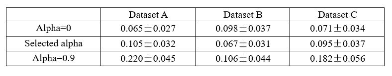
(4) Synthetic experiments can effectively rule out the leakage scenario.
In the absence of ground truth data, synthetic experiments serve as an effective method for validating models and are commonly employed [1-3].
Our experimental results demonstrate that d-VAE can effectively extract neural signals that more closely resemble actual behaviorally relevant signals (Fig. S2g). If there were information leakage, it would decrease the similarity to the ground truth signals, hence we have ruled out this possibility. Moreover, in synthetic experiments with small R2 neurons (Fig. S10), results also demonstrate that our model could make these neurons more closely resemble ground truth relevant signals and recover their information.
In summary, synthetic experiments strongly demonstrate that our model can recover obscured neuronal information, rather than adding signals that do not exist.
(1) Pnevmatikakis, Eftychios A., et al. "Simultaneous denoising, deconvolution, and demixing of calcium imaging data." Neuron 89.2 (2016): 285-299.
(2) Schneider, Steffen, Jin Hwa Lee, and Mackenzie Weygandt Mathis. "Learnable latent embeddings for joint behavioural and neural analysis." Nature 617.7960 (2023): 360-368.
(3) Zhou, Ding, and Xue-Xin Wei. "Learning identifiable and interpretable latent models of high-dimensional neural activity using pi-VAE." Advances in Neural Information Processing Systems 33 (2020): 7234-7247.
Based on these four points, we are confident in the reliability of our results. If Reviewer #4 considers these points insufficient, we would highly appreciate it if specific concerns regarding any of these aspects could be detailed.
Thank you for your valuable feedback.
Q5: “Given the nuances involved in appropriate comparisons across methods and since two of the datasets are public, the authors should provide their complete code (not just the dVAE method code), including the code for data loading, data preprocessing, model fitting and model evaluation for all methods and public datasets. This will alleviate concerns and allow readers to confirm conclusions (e.g., figure 2) for themselves down the line.”
Thanks for your suggestion.
Our codes are now available on GitHub at https://github.com/eric0li/d-VAE. Thank you for your valuable feedback.
Q6: “Related to 1) above, the authors should explore the results if the affine network h(.) (from embedding to behavior) was replaced with a nonlinear ANN. Perhaps linear decoders would no longer be as close to nonlinear decoders. Regardless, the claim of linearity should be revised as described in 1) and 2) above, and all caveats should be discussed.”
Thank you for your suggestion. We appreciate your feasible proposal that can be empirically tested. Following your suggestion, we have replaced the decoding of the latent variable z to behavior y with a nonlinear neural network, specifically a neural network with a single hidden layer. The modified model is termed d-VAE2. We applied the d-VAE2 to the real data, and selected the optimal alpha through the validation set. As shown in Table 1, results demonstrate that the performance of KF and ANN remains comparable. Therefore, the capacity to linearly decode behaviorally relevant signals does not stem from the linear decoding of embeddings.
Author response table 2.
Decoding R2 of behaviorally relevant signals obtained by d-VAE2
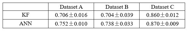
Additionally, it is worth noting that this approach is uncommon and is considered somewhat inappropriate according to the Information Bottleneck theory [1]. According to the Information Bottleneck theory, information is progressively compressed in multilayer neural networks, discarding what is irrelevant to the output and retaining what is relevant. This means that as the number of layers increases, the mutual information between each layer's embedding and the model input gradually decreases, while the mutual information between each layer's embedding and the model output gradually increases. For the decoding part, if the embeddings that is not closest to the output (behaviors) is used, then these embeddings might contain behaviorally irrelevant signals. Using these embeddings to generate behaviorally relevant signals could lead to the inclusion of irrelevant signals in the behaviorally relevant signals.
To demonstrate the above statement, we conducted experiments on the synthetic data. As shown in Table 2, we present the performance (neural R2 between the generated signals and the ground truth signals) of both models at several alpha values around the optimal alpha of dVAE (alpha=0.9) selected by the validation set. The experimental results show that at the same alpha value, the performance of d-VAE2 is consistently inferior to that of d-VAE, and d-VAE2 requires a higher alpha value to achieve performance comparable to d-VAE, and the best performance of d-VAE2 is inferior to that of d-VAE.
Author response table 3.
Neural R2 between generated signals and real behaviorally relevant signals
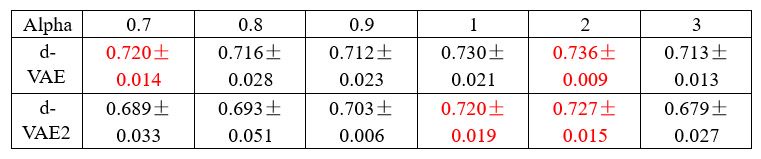
Thank you for your valuable feedback.
(1) Shwartz-Ziv, Ravid, and Naftali Tishby. "Opening the black box of deep neural networks via information." arXiv preprint arXiv:1703.00810 (2017).
Q7: “The beginning of the section on the "smaller R2 neurons" should clearly define what R2 is being discussed. Based on the response to previous reviewers, this R2 "signifies the proportion of neuronal activity variance explained by the linear encoding model, calculated using raw signals". This should be mentioned and made clear in the main text whenever this R2 is referred to.”
Thank you for your suggestion. We have made the modifications in the main text. Thank you for your valuable feedback.
Q8: “Various terms require clear definitions. The authors sometimes use vague terminology (e.g., "useless") without a clear definition. Similarly, discussions regarding dimensionality could benefit from more precise definitions. How is neural dimensionality defined? For example, how is "neural dimensionality of specific behaviors" (line 590) defined? Related to this, I agree with Reviewer 2 that a clear definition of irrelevant should be mentioned that clarifies that relevance is roughly taken as "correlated or predictive with a fixed time lag". The analyses do not explore relevance with arbitrary time lags between neural and behavior data.”
Thanks for your suggestion. We have removed the “useless” statements and have revised the statement of “the neural dimensionality of specific behaviors” in our revised manuscripts.
Regarding the use of fixed temporal lags, we followed the same practice as papers related to the dataset we use, which assume fixed temporal lags [1-3]. Furthermore, many studies in the motor cortex similarly use fixed temporal lags [4-6]. To clarify the definition, we have revised the definition in our manuscript. For details, please refer to the response to Q2 of reviewer #2 and our revised manuscript. We believe our definition is clearly articulated.
Thank you for your valuable feedback.
(1) Wang, Fang, et al. "Quantized attention-gated kernel reinforcement learning for brain– machine interface decoding." IEEE transactions on neural networks and learning systems 28.4 (2015): 873-886.
(2) Dyer, Eva L., et al. "A cryptography-based approach for movement decoding." Nature biomedical engineering 1.12 (2017): 967-976.
(3) Ahmadi, Nur, Timothy G. Constandinou, and Christos-Savvas Bouganis. "Robust and accurate decoding of hand kinematics from entire spiking activity using deep learning." Journal of Neural Engineering 18.2 (2021): 026011.
(4) Churchland, Mark M., et al. "Neural population dynamics during reaching." Nature 487.7405 (2012): 51-56.
(5) Kaufman, Matthew T., et al. "Cortical activity in the null space: permitting preparation without movement." Nature neuroscience 17.3 (2014): 440-448.
(6) Elsayed, Gamaleldin F., et al. "Reorganization between preparatory and movement population responses in motor cortex." Nature communications 7.1 (2016): 13239.
Q9: “CEBRA itself doesn't provide a neural reconstruction from its embeddings, but one could obtain one via a regression from extracted CEBRA embeddings to neural data. In addition to decoding results of CEBRA (figure S3), the neural reconstruction of CEBRA should be computed and CEBRA should be added to Figure 2 to see how the behaviorally relevant and irrelevant signals from CEBRA compare to other methods.”
Thank you for your question. Modifying CEBRA is beyond the scope of our work. As CEBRA is not a generative model, it cannot obtain behaviorally relevant and irrelevant signals, and therefore it lacks the results presented in Fig. 2. To avoid the same confusion encountered by reviewers #3 and #4 among our readers, we have opted to exclude the comparison with CEBRA. It is crucial to note, as previously stated, that our assessment of decoding capabilities has been benchmarked against the performance of the ANN on raw signals, which almost represents the upper limit of performance. Consequently, omitting CEBRA does not affect our conclusions.
Thank you for your valuable feedback.
Q10: “Line 923: "The optimal hyperparameter is selected based on the lowest averaged loss of five-fold training data." => why is this explained specifically under CEBRA? Isn't the same criteria used for hyperparameters of other methods? If so, clarify.”
Thank you for your question. The hyperparameter selection for CEBRA follows the practice of the original CEBRA paper. The hyperparameter selection for generative models is detailed in the Section “The strategy for selecting effective behaviorally-relevant signals”. Thank you for your valuable feedback.
Author Response
The following is the authors’ response to the previous reviews.
Reviewer #2 (Public Review):
Summary:
In the revised manuscript, the authors aim to investigate brain-wide activation patterns following administration of the anesthetics ketamine and isoflurane, and conduct comparative analysis of these patterns to understand shared and distinct mechanisms of these two anesthetics. To this end, they perform Fos immunohistochemistry in perfused brain sections to label active nuclei, use a custom pipeline to register images to the ABA framework and quantify Fos+ nuclei, and perform multiple complementary analyses to compare activation patterns across groups.
In the latest revision, the authors have made some changes in response to our previous comments on how to fix the analyses. However, the revised analyses were not changed correctly and remain flawed in several fundamental ways.
Critical problems:
(1) Before one can perform higher level analyses such as hiearchal cluster or network hub (or PC) analysis, it is fundamental to validate that you have significant differences of the raw Fos expression values in the first place. First of all, this means showing figures with the raw data (Fos expression levels) in some form in Figures 2 and 3 before showing the higher level analyses in Figures 4 and 5; this is currently switched around. Second and most importantly, when you have a large number of brain areas with large differences in mean values and variance, you need to account for this in a meaningful way. Changing to log values is a step in the right direction for mean values but does not account well for differences in variance. Indeed, considering the large variances in brain areas with high mean values and variance, it is a little difficult to believe that all brain regions, especially brain areas with low mean values, passed corrections for multiple comparisons test. We suggested Z-scores relative to control values for each brain region; this would have accounted for wide differences in mean values and variance, but this was not done. Overall, validation of anesthesia-induced differences in Fos expression levels is not yet shown.
(a) Reordering the figures.
Thank you for your suggestion. We have added Figure 2 (for 201 brain regions) and Figure 2—figure supplement 1 (for 53 brain regions) to demonstrate the statistical differences in raw Fos expression between KET and ISO compared to their respective control groups. These figures specifically present the raw c-Fos expression levels for both KET and ISO in the same brain areas, providing a fundamental basis for the subsequent analyses. Additionally, we have moved the original Figures 4 and 5 to Figures 3 and 4.
(b) Z-score transformation and validation of anesthesia-induced differences in Fos expression.
Thank you for your suggestion. Before multiple comparisons, we transformed the data into log c-Fos density and then performed Z-scores relative to control values for each brain region. Indeed, through Z-score transformation, we have identified a larger number of significantly activated brain regions in Figure 2. The number of brain regions showing significant activation increased by 100 for KET and by 39 for ISO. We have accordingly updated the results section to include these findings in Line 80-181. Besides, we have added the following content in the Statistical Analysis section in Line 489: "…In Figure 2 and Figure 2–figure supplement 1, c-Fos densities in both experimental and control groups were log-transformed. Z-scores were calculated for each brain region by normalizing these log-transformed values against the mean and standard deviation of its respective control group. This involved subtracting the control mean from the experimental value and dividing the result by the control standard deviation. For statistical analysis, Z-scores were compared to a null distribution with a zero mean, and adjustments were made for multiple comparisons using the Benjamini–Hochberg method with a 5% false discovery rate (Q)..…".
Author response image 1.
KET and ISO induced c-Fos expression relative to their respective control group across 201 distinct brain regions. Z-scores represent the normalized c-Fos expression in the KET and ISO groups, calculated against the mean and standard deviation from their respective control groups. Statistical analysis involved the comparison of Z-scores to a null distribution with a zero mean and adjustment for multiple comparisons using the Benjamini–Hochberg method at a 5% false discovery rate (p < 0.05, p < 0.01, **p < 0.001). n = 6, 6, 8, 6 for the home cage, ISO, saline, and KET, respectively. Missing values resulted from zero standard deviations in control groups. Brain regions are categorized into major anatomical subdivisions, as shown on the left side of the graph.
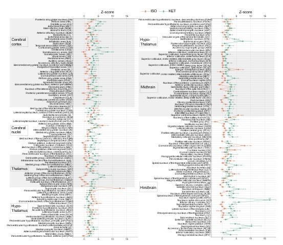
Author response image 2.
KET and ISO induced c-Fos expression relative to their respective control group across 53 distinct brain regions. Z-scores for c-Fos expression in the KET and ISO groups were normalized to the mean and standard deviation of their respective control groups. Statistical analysis involved the comparison of Z-scores to a null distribution with a zero mean and adjustment for multiple comparisons using the Benjamini–Hochberg method at a 5\% false discovery rate (p < 0.05, p < 0.01, **p < 0.001). Brain regions are organized into major anatomical subdivisions, as indicated on the left side of the graph.
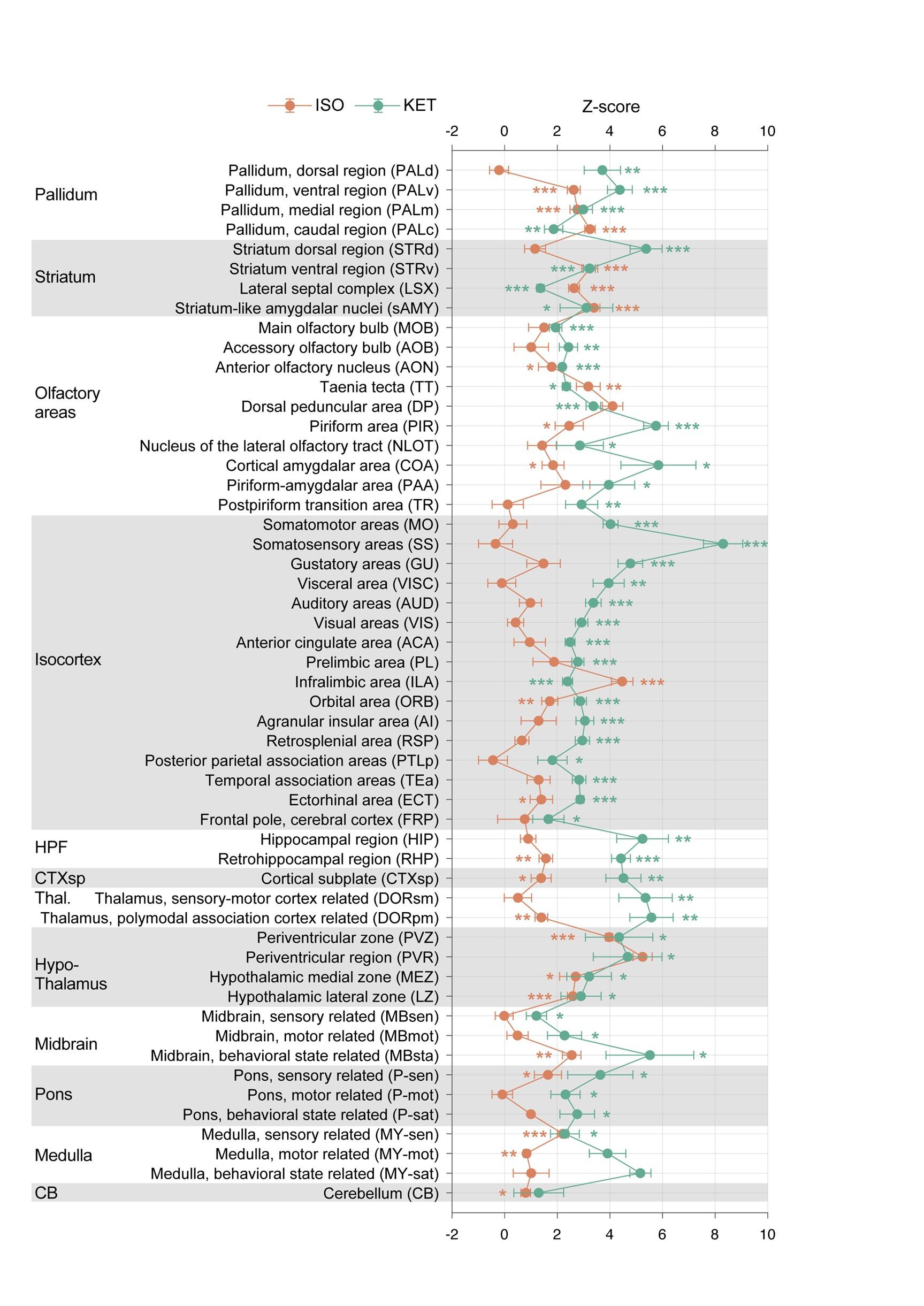
(2) Let's assume for a moment that the raw Fos expression analyses indicate significant differences. They used hierarchal cluster analyses as a rationale for examining 53 brain areas in all subsequent analyses of Fos expression following isoflurane versus home cage or ketamine versus saline. Instead, the authors changed to 201 brain areas with no validated rationale other than effectively saying 'we wanted to look at more brain areas'. And then later, when they examined raw Fos expression values in Figures 4 and 5, they assess 43 brain areas for ketamine and 20 brain areas for isoflurane, without any rationale for why choosing these numbers of brain areas. This is a particularly big problem when they are trying to compare effects of isoflurane versus ketamine on Fos expression in these brain areas - they did not compare the same brain areas.
(a) Changing to 201 brain areas with validated rationale.
Thank you for your question. We have revised the original text from “To enhance our analysis of c-Fos expression patterns induced by KET and ISO, we expanded our study to 201 subregions.” to Line 100: "…To enable a more detailed examination and facilitate clearer differentiation and comparison of the effects caused by KET and ISO, we subdivided the 53 brain regions into 201 distinct areas. This approach, guided by the standard mouse atlas available at http://atlas.brain-map.org/atlas, allowed for an in-depth analysis of the responses in various brain regions…". For hierarchal cluster analyses from 53 to 201 brain regions, Line 215: "…To achieve a more granular analysis and better discern the responses between KET and ISO, we expanded our study from the initial 53 brain regions to 201 distinct subregions…"
(b) Compare the same brain areas for KET and ISO and the rationale for why choosing these numbers of brain areas in Figures 3 and 4.
We apologize for the confusion and lack of clarity regarding the selection of brain regions for analysis. In Figure 2 and Figure 2—figure supplement 1, we display the c-Fos expression in the same brain regions affected by KET and ISO. In Figures 3 and 4, we applied a uniform standard to specifically report the brain areas most prominently activated by KET and ISO, respectively. As specified in Line 104: "…Compared to the saline group, KET activated 141 out of a total of 201 brain regions (Figure 2). To further identify the brain regions that are most significantly affected by KET, we calculated Cohen's d for each region to quantify the magnitude of activation and subsequently focused on those regions that had a corrected p-value below 0.05 and effect size in the top 40% (Figure 3, Figure 3—figure supplement 1)…" and Line 142: "…Using the same criteria applied to KET, which involved selecting regions with Cohen's d values in the top 40% of significantly activated areas from Figure 2, we identified 32 key brain regions impacted by ISO (Figure 4, Figure 4—figure supplement 1).…".
Moreover, we illustrate the co-activated brain regions by KET and ISO in Figure 4C. As detailed in Lines 167-180:"…The co-activation of multiple brain regions by KET and ISO indicates that they have overlapping effects on brain functions. Examples of these effects include impacts on sensory processing, as evidenced by the activation of the PIR, ENT 1, and OT2, pointing to changes in sensory perception typical of anesthetics. Memory and cognitive functions are influenced, as indicated by the activation of the subiculum (SUB) 3, dentate gyrus (DG) 4, and RE 5. The reward and motivational systems are engaged, involving the ACB and ventral tegmental area (VTA), signaling the modulation of reward pathways 6. Autonomic and homeostatic control are also affected, as shown by areas like the lateral hypothalamic area (LHA) 7 and medial preoptic area (MPO) 8, emphasizing effects on functions such as feeding and thermoregulation. Stress and arousal responses are impacted through the activation of the paraventricular hypothalamic nucleus (PVH) 10,11 and LC 12. This broad activation pattern highlights the overlap in drug effects and the complexity of brain networks in anesthesia…". Below are the revised Figures 3 and 4.
(1) Chapuis, J. et al. Lateral entorhinal modulation of piriform cortical activity and fine odor discrimination. J. Neurosci. 33, 13449-13459 (2013). https://doi.org:10.1523/jneurosci.1387-13.2013
(2) Giessel, A. J. & Datta, S. R. Olfactory maps, circuits and computations. Curr. Opin. Neurobiol. 24, 120-132 (2014). https://doi.org:10.1016/j.conb.2013.09.010
(3) Roy, D. S. et al. Distinct Neural Circuits for the Formation and Retrieval of Episodic Memories. Cell 170, 1000-1012.e1019 (2017). https://doi.org:10.1016/j.cell.2017.07.013
(4) Sun, X. et al. Functionally Distinct Neuronal Ensembles within the Memory Engram. Cell 181, 410-423.e417 (2020). https://doi.org:10.1016/j.cell.2020.02.055
(5) Huang, X. et al. A Visual Circuit Related to the Nucleus Reuniens for the Spatial-Memory-Promoting Effects of Light Treatment. Neuron (2021).
(6) Al-Hasani, R. et al. Ventral tegmental area GABAergic inhibition of cholinergic interneurons in the ventral nucleus accumbens shell promotes reward reinforcement. Nat. Neurosci. 24, 1414-1428 (2021). https://doi.org:10.1038/s41593-021-00898-2
(7) Mickelsen, L. E. et al. Single-cell transcriptomic analysis of the lateral hypothalamic area reveals molecularly distinct populations of inhibitory and excitatory neurons. Nat. Neurosci. 22, 642-656 (2019). https://doi.org:10.1038/s41593-019-0349-8
(8) McGinty, D. & Szymusiak, R. Keeping cool: a hypothesis about the mechanisms and functions of slow-wave sleep. Trends Neurosci. 13, 480-487 (1990). https://doi.org:10.1016/0166-2236(90)90081-k
(9) Mullican, S. E. et al. GFRAL is the receptor for GDF15 and the ligand promotes weight loss in mice and nonhuman primates. Nat. Med. 23, 1150-1157 (2017). https://doi.org:10.1038/nm.4392
(10) Rasiah, N. P., Loewen, S. P. & Bains, J. S. Windows into stress: a glimpse at emerging roles for CRH(PVN) neurons. Physiol. Rev. 103, 1667-1691 (2023). https://doi.org:10.1152/physrev.00056.2021
(11) Islam, M. T. et al. Vasopressin neurons in the paraventricular hypothalamus promote wakefulness via lateral hypothalamic orexin neurons. Curr. Biol. 32, 3871-3885.e3874 (2022). https://doi.org:10.1016/j.cub.2022.07.020
(12) Ross, J. A. & Van Bockstaele, E. J. The Locus Coeruleus- Norepinephrine System in Stress and Arousal: Unraveling Historical, Current, and Future Perspectives. Front Psychiatry 11, 601519 (2020). https://doi.org:10.3389/fpsyt.2020.601519
Author response image 3.
Brain regions exhibiting significant activation by KET. (A) Fifty-five brain regions exhibited significant KET activation. These were chosen from the 201 regions analyzed in Figure 2, focusing on the top 40\% ranked by effect size among those with corrected p values less than 0.05. Data are presented as mean ± SEM, with p-values adjusted for multiple comparisons (p < 0.05, p < 0.01, **p < 0.001). (B) Representative immunohistochemical staining of brain regions identified in Figure 3A, with control group staining available in Figure 3—figure supplement 1. Scale bar: 200 µm.
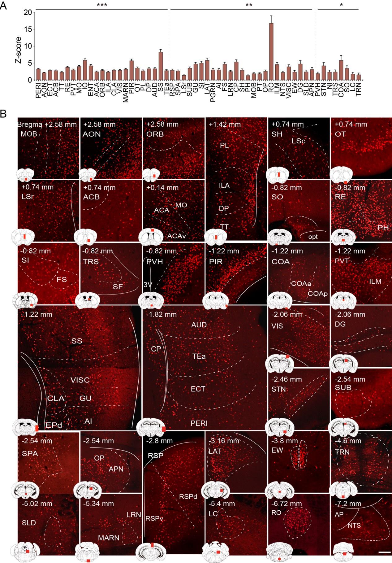
Author response image 4.
Brain regions exhibiting significant activation by ISO. (A) Brain regions significantly activated by ISO were initially identified using a corrected p-value below 0.05. From these, the top 40% in effect size (Cohen’s d) were further selected, resulting in 32 key areas. p-values are adjusted for multiple comparisons (p < 0.01, *p < 0.001). (B) Representative immunohistochemical staining of brain regions identified in Figure 4A. Control group staining is available in Figure 4—figure supplement 1. Scale bar: 200 µm. Scale bar: 200 µm. (C) A Venn diagram displays 43 brain regions co-activated by KET and ISO, identified by the adjusted p-values (p < 0.05) for both KET and ISO. CTX: cerebral cortex; CNU: cerebral nuclei; TH: thalamus; HY: hypothalamus; MB: midbrain; HB: hindbrain.
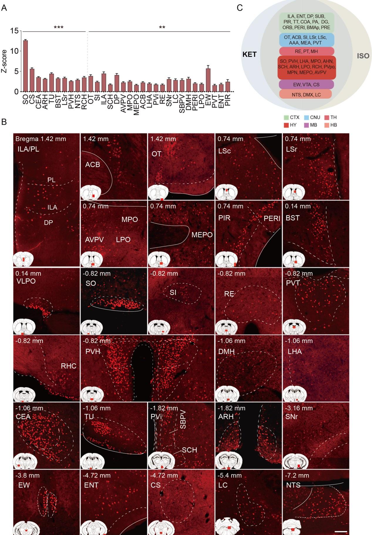
Less critical comments:
(3) The explanation of hierarchical level's in lines 90-95 did not make sense.
We have revised the section that initially stated in lines 90-95, "…Based on the standard mouse atlas available at http://atlas.brain-map.org/, the mouse brain was segmented into nine hierarchical levels, totaling 984 regions. The primary level consists of grey matter, the secondary of the cerebrum, brainstem, and cerebellum, and the tertiary includes regions like the cerebral cortex and cerebellar nuclei, among others, with some regions extending to the 8th and 9th levels. The fifth level comprises 53 subregions, with detailed expression levels and their respective abbreviations presented in Supplementary Figure 2…". Our revised description, now in line 91: "…Building upon the framework established in previous literature, our study categorizes the mouse brain into 53 distinct subregions1…"
(1) Do JP, Xu M, Lee SH, Chang WC, Zhang S, Chung S, Yung TJ, Fan JL, Miyamichi K, Luo L et al: Cell type-specific long-range connections of basal forebrain circuit. Elife 2016, 5.
(4) I am still perplexed by why the authors consider the prelimbic and infralimbic cortex 'neuroendocrine' brain areas in the abstract. In contrast, the prelimbic and infralimbic were described better in the introduction as "associated information processing" areas.
Thank you for bringing this to our attention. We agree that classifying the prelimbic and infralimbic cortex as 'neuroendocrine' in the abstract was incorrect, which was an oversight on our part. In the revised version, as detailed in line 167, we observed an increased number of brain regions showing overlapping activation by both KET and ISO, which is depicted in Figure 4C. This extensive co-activation across various regions makes it challenging to narrowly define the functional classification of each area. Consequently, we have revised the abstract, updating this in line 21: "…KET and ISO both activate brain areas involved in sensory processing, memory and cognition, reward and motivation, as well as autonomic and homeostatic control, highlighting their shared effects on various neural pathways.…".
(5) It looks like overall Fos levels in the control group Home (ISO) are a magnitude (~10-fold) lower than those in the control group Saline (KET) across all regions shown. This large difference seems unlikely to be due to a biologically driven effect and seems more likely to be due to a technical issue, such as differences in staining or imaging between experiments. The authors discuss this issue but did not answer whether the Homecage-ISO experiment or at least the Fos labeling and imaging performed at the same time as for the Saline-Ketamine experiment?
Thank you for highlighting this important point. The c-Fos labeling and imaging for the Home (ISO) and Saline (KET) groups were carried out in separate sessions due to the extensive workload involved in these processes. This study processed a total of 26 brain samples. Sectioning the entire brain of each mouse required approximately 3 hours, yielding 5 slides, with each slide containing 12 to 16 brain sections. We were able to stain and image up to 20 slides simultaneously, typically comprising 2 experimental groups and 2 corresponding control groups. Imaging these 20 slides at 10x magnification took roughly 7 hours, while additional time was required for confocal imaging of specific areas of interest at 20x magnification. Given the complexity of these procedures, to ensure consistency across all experiments, they were conducted under uniform conditions. This included the use of consistent primary and secondary antibody concentrations, incubation times, and imaging parameters such as fixed light intensity and exposure time. Furthermore, in the saline and KET groups, intraperitoneal injections might have evoked pain and stress responses in mice despite four days of pre-experiment acclimation, which could have contributed to the increased c-Fos expression observed. This aspect, along with the fact that procedures were conducted in separate sessions, might have introduced some variations. Thus, we have included a note in our discussion section in Line 353: "…Despite four days of acclimation, including handling and injections, intraperitoneal injections in the saline and KET groups might still elicit pain and stress responses in mice. This point is corroborated by the subtle yet measurable variations in brain states between the home cage and saline groups, characterized by changes in normalized EEG delta/theta power (home cage: 0.05±0.09; saline: -0.03±0.11) and EMG power (home cage: -0.37±0.34; saline: 0.04±0.13), as shown in Figure 1–figure supplement 1. These changes suggest a relative increase in brain activity in the saline group compared to the home cage group, potentially contributing to the higher c-Fos expression. Additionally, despite the use of consistent parameters for c-Fos labeling and imaging across all experiments, the substantial differences observed between the saline and home cage groups might be partly attributed to the fact that the operations were conducted in separate sessions.…"
Reviewer #3 (Public Review):
The present study presents a comprehensive exploration of the distinct impacts of Isoflurane and Ketamine on c-Fos expression throughout the brain. To understand the varying responses across individual brain regions to each anesthetic, the researchers employ principal component analysis (PCA) and c-Fos-based functional network analysis. The methodology employed in this research is both methodical and expansive. Notably, the utilization of a custom software package to align and analyze brain images for c-Fos positive cells stands out as an impressive addition to their approach. This innovative technique enables effective quantification of neural activity and enhances our understanding of how anesthetic drugs influence brain networks as a whole.
The primary novelty of this paper lies in the comparative analysis of two anesthetics, Ketamine and Isoflurane, and their respective impacts on brain-wide c-Fos expression. The study reveals the distinct pathways through which these anesthetics induce loss of consciousness. Ketamine primarily influences the cerebral cortex, while Isoflurane targets subcortical brain regions. This finding highlights the differing mechanisms of action employed by these two anesthetics-a top-down approach for Ketamine and a bottom-up mechanism for Isoflurane. Furthermore, this study uncovers commonly activated brain regions under both anesthetics, advancing our knowledge about the mechanisms underlying general anesthesia.
We are thankful for your positive and insightful comments on our study. Your recognition of the study's methodology and its significance in advancing our understanding of anesthetic mechanisms is greatly valued. By comprehensively mapping c-Fos expression across a wide range of brain regions, our study reveals the distinct and overlapping impacts of these anesthetics on various brain functions, providing a valuable foundation for future research into the mechanisms of general anesthesia, potentially guiding the development of more targeted anesthetic agents and therapeutic strategies. Thus, we are confident that our work will captivate the interest of our readers.
Author Response
The following is the authors’ response to the previous reviews.
We appreciate the reviewers for their insightful feedback, which has substantially improved our manuscript. Following the suggestions of the reviewers, we have undertaken the following major revisions:
a. Concerning data transformation, we have adjusted the methodology in Figures 2 and 3. Instead of normalizing c-Fos density to the whole brain c-Fos density as initially described, we now normalize to the c-Fos density of the corresponding brain region in the control group. b. We have substituted the PCA approach with hierarchical clustering in Figures 2 and 3.
c. In the discussion section, we added a subsection on study limitations, focusing on the variations in drug administration routes and anesthesia depth.
Enclosed are our detailed responses to each of the reviewer's comments.
Reviewer #1:
1a. The addition of the EEG/EMG is useful, however, this information is not discussed. For instance, there are differences in EEG/EMG between the two groups (only Ket significantly increased delta/theta power, and only ISO decreased EMG power). These results should be discussed as well as the limitation of not having physiological measures of anesthesia to control for the anesthesia depth.
1b. The possibility that the differences in fos observed may be due to the doses used should be discussed.
1c. The possibility that the differences in fos observed may be due kinetic of anesthetic used should be discussed.
Thank you for your suggestions. We have now discussed EEG/EMG result, limitation of not having physiological measures of anesthesia to control for the anesthesia depth, The possibility that the differences in fos observed may be due to the doses, The possibility that the differences in Fos observed may be due kinetic of anesthetic in the revised manuscript (Lines 308-331, also shown below).
Lines 308-331: "...Our findings indicate that c-Fos expression in the KET group is significantly elevated compared to the ISO group, and the saline group exhibits notably higher c-Fos expression than the home cage group, as seen in Supplementary Figures 2 and 3. Intraperitoneal saline injections in the saline group, despite pre-experiment acclimation with handling and injections for four days, may still evoke pain and stress responses in mice. Subtle yet measurable variations in brain states between the home cage and saline groups were observed, characterized by changes in normalized EEG delta/theta power (home cage: 0.05±0.09; saline: -0.03±0.11) and EMG power (home cage: -0.37±0.34; saline: 0.04±0.13), as shown in Supplementary Figure 1. These changes suggest a relative increase in overall brain activity in the saline group compared to the home cage group, potentially contributing to the higher c-Fos expression. Although the difference in EEG power between the ISO group and the home cage control was not significant, the increase in EEG power observed in the ISO group was similar to that of KET (0.47 ± 0.07 vs 0.59 ± 0.10), suggesting that both agents may induce loss of consciousness in mice. Regarding EMG power, ISO showed a significant decrease in EMG power compared to its control group. In contrast, the KET group showed a lesser reduction in EMG power (ISO: -1.815± 0.10; KET: -0.96 ± 0.21), which may partly explain the higher overall c-Fos expression levels in the KET group. This is consistent with previous studies where ketamine doses up to 150 mg/kg increase delta power while eliciting a wakefulness-like pattern of c-Fos expression across the brain [1]. Furthermore, the observed differences in c-Fos expression may arise in part from the dosages, routes of administration, and their distinct pharmacokinetic profiles. This variation is compounded by the lack of detailed physiological monitoring, such as blood pressure, heart rate, and respiration, affecting our ability to precisely assess anesthesia depth. Future studies incorporating comprehensive physiological monitoring and controlled dosing regimens are essential to further elucidate these relationships and refine our understanding of the effects of anesthetics on brain activity"
2b. I am confused because Fig 2C seems to show significant decrease in %fos in the hypothalamus, midbrain and cerebellum after KET, while the author responded that " in our analysis, we did not detect regions with significant downregulation when comparing anesthetized mice with controls." Moreover the new figure in the rebuttal in response to reviewer 2 suggests that Ket increases Fos in almost every single region (green vs blue) which is not the conclusion of the paper.
Your concern regarding the apparent discrepancy is well-founded. The inconsistency arose due to an inappropriate data transformation, which affected the interpretation. We have now rectified this by adjusting the data transformation in Figures 2 and 3. Specifically, we have recalculated the log relative c-Fos density values relative to the control group for each brain region. This revision has resolved the issue, confirming that our analysis did not detect any regions with significant downregulation in the anesthetized mice compared to controls. We have also updated the results, discussion, and methods sections of Figures 2 and 3 to accurately reflect these changes and ensure consistency with our findings.
Author response image 1.
Figure 2. Whole-brain distributions of c-Fos+ cells induced by ISO and KET. (A) Hierarchical clustering was performed on the log relative c-Fos density data for ISO and KET using the complete linkage method based on the Euclidean distance matrix, with clusters identified by a dendrogram cut-off ratio of 0.5. Numerical labels correspond to distinct clusters within the dendrogram. (B) Silhouette values plotted against the ratio of tree height for ISO and KET, indicating relatively higher Silhouette values at 0.5 (dashed line), which is associated with optimal clustering. (C) The number of clusters identified in each treatment condition at different ratios of the dendrogram tree height, with a cut-off level of 0.5 corresponding to 4 clusters for both ISO and KET (indicated by the dashed line). (D) The bar graph depicts Z scores for clusters in ISO and KET conditions, represented with mean values and standard errors. One-way ANOVA with Tukey's post hoc multiple comparisons. ns: no significance; ***P < 0.001. (E) Z-scored log relative density of c-Fos expression in the clustered brain regions. The order and abbreviations of the brain regions and the numerical labels correspond to those in Figure 2A. The red box denotes the cluster with the highest mean Z score in comparison to other clusters. CTX: cortex; TH: thalamus; HY: hypothalamus; MB: midbrain; HB: hindbrain.
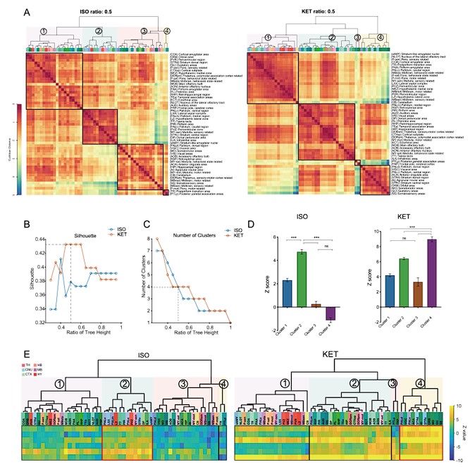
Author response image 2.
Figure 3. Similarities and differences in ISO and KET activated c-Fos brain areas. (A) Hierarchical clustering was performed on the log-transformed relative c-Fos density data for ISO and KET using the complete linkage method based on the Euclidean distance matrix, with clusters identified by a dendrogram cut-off ratio of 0.5. (B) Silhouette values are plotted against the ratio of tree height from the hierarchical clustered dendrogram in Figure 3A. (C) The relationship between the number of clusters and the tree height ratio of the dendrogram for ISO and KET, with a cut-off ratio of 0.5 resulting in 3 clusters for ISO and 5 for KET (indicated by the dashed line). (D) The bar graph depicts Z scores for clusters in ISO and KET conditions, represented with mean values and standard errors. One-way ANOVA with Tukey's post hoc multiple comparisons. ns: no significance; ***P < 0.001. (E) Z-scored log relative density of c-Fos expression within the identified brain region clusters. The arrangement, abbreviations of the brain regions, and the numerical labels are in accordance with Figure 3A. The red boxes highlight brain regions that rank within the top 10 percent of Z score values. The white boxes denote brain regions with an Z score less than -2.
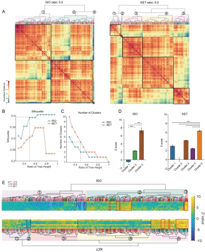
- There are still critical misinterpretations of the PCA analysis. For instance, it is mentioned that " KET is associated with the activation of cortical regions (as evidenced by positive PC1 coefficients in MOB, AON, MO, ACA, and ORB) and the inhibition of subcortical areas (indicated by negative coefficients) " as well as " KET displays cortical activation and subcortical inhibition, whereas ISO shows a contrasting preference, activating the cerebral nucleus (CNU) and the hypothalamus while inhibiting cortical areas. To reduce inter-individual variability." These interpretations are in complete contradiction with the answer 2b above that there was no region that had decreased Fos by either anesthetic.
Thank you for bringing this to our attention. In response to your concerns, we have made significant revisions to our data analysis. We have updated our input data to incorporate log-transformed relative c-Fos density values, normalized against the control group for each brain region, as illustrated in Figures 2 and 3. Instead of PCA, we have applied this updated data to hierarchical clustering analysis. The results of these analyses are consistent with our original observation that neither anesthetic led to a decrease in Fos expression in any region.
- I still do not understand the rationale for the use of that metric. The use of a % of total Fos makes the data for each region dependent on the data of the other regions which wrongly leads to the conclusion that some regions are inhibited while they are not when looking at the raw data. Moreover, the interdependence of the variable (relative density) may affect the covariance structure which the PCA relies upon. Why not using the PCA on the logarithm of the raw data or on a relative density compared to the control group on a region-per-region basis instead of the whole brain?
Thank you for your insightful suggestion. Following your advice, we have revised our approach and now utilize the logarithm of the relative density compared to the control group on a region-by-region basis. We attempted PCA analyses using the logarithm of the raw data, the logarithm of the Z-score, and the logarithm of the relative density compared to control, but none yielded distinct clusters.
Author response image 3.
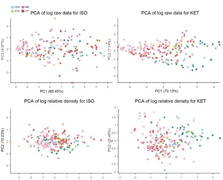
As a result, we employed hierarchical cluster analysis. We then examined the Z-scores of the log-transformed relative c-Fos densities (Figures 2E and 3E) to assess expression levels across clusters. Our analysis revealed that neither ISO nor KET treatments led to a significant suppression of c-Fos expression in the 53 brain regions examined. In the ISO group alone, there were 10 regions that demonstrated relative suppression (Z-score < -2, indicated by white boxes) as shown in Figure 3.
Fig. 2B: it's unclear to me why the regions are connected by a line. Such representation is normally used for time series/within-subject series. What is the rationale for the order of the regions and the use of the line? The line connecting randomly organized regions is meaningless and confusing.
Thank you for your suggestion. We have discontinued the use of PCA calculations and have removed this figure.
Fig 6A. The correlation matrices are difficult to interpret because of the low resolution and arbitrary order of brain regions. I recommend using hierarchical clustering and/or a combination of hierarchical clustering and anatomical organization (e.g. PMID: 31937658). While it is difficult to add the name of the regions on the graph I recommend providing supplementary figures with large high-resolution figures with the name of each brain region so the reader can actually identify the correlation between specific brain regions and the whole brain, Rationale for Metric Choice: Note that I do not dispute the choice of the log which is appropriate, it is the choice of using the relative density that I am questioning.
Thank you for your constructive feedback. In line with your suggestion, we have implemented hierarchical clustering combined with anatomical organization as per the referenced literature. Additionally, we have updated the vector diagrams in Figure 6A to present them with greater clarity.
Furthermore, we have revised our network modular division method based on cited literature recommendations. We used hierarchical clustering with correlation coefficients to segment the network into modules, illustrated in Figure 6—figure supplement 1. Due to the singular module structure of the KET network and the sparsity of intermodular connections in the home cage and saline networks, the assessment of network hub nodes did not employ within-module degree Z-score and participation coefficients, as these measures predominantly underscore the importance of connections within and between modules. Instead, we used degree, betweenness centrality, and eigenvector centrality to detect the hub nodes, as detailed in Figure 6—figure supplement 2. With this new approach, the hub node for the KET condition changed from SS to TeA. Corresponding updates have been made to the results section for Figure 6, as well as to the related discussions and the abstract of our paper.
Author response image 4.
Figure 6. Generation of anesthetics-induced networks and identification of hub regions. (A) Heatmaps display the correlations of log c-Fos densities within brain regions (CTX, CNU, TH, HY, MB, and HB) for various states (home cage, ISO, saline, KET). Correlations are color-coded according to Pearson's coefficients. The brain regions within each anatomical category are organized by hierarchical clustering of their correlation coefficients. (B) Network diagrams illustrate significant positive correlations (P < 0.05) between regions, with Pearson’s r exceeding 0.82. Edge thickness indicates correlation magnitude, and node size reflects the number of connections (degree). Node color denotes betweenness centrality, with a spectrum ranging from dark blue (lowest) to dark red (highest). The networks are organized into modules consistent with the clustering depicted in Supplementary Figure 8. Figure 6—figure supplement 1
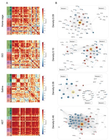
Author response image 5.
Figure 6—figure supplement 1. Hierarchical clustering of brain regions under various conditions: home cage, ISO, saline, and KET. (A) Heatmaps show the relative distances among brain regions assessed in naive mice. Modules were identified by sectioning each dendrogram at a 0.7 threshold. (B) Silhouette scores plotted against the dendrogram tree height ratio for each condition, with optimal cluster definition indicated by a dashed line at a 0.7 ratio. (C) The number of clusters formed at different cutoff levels. At a ratio of 0.7, ISO and saline treatments result in three clusters, whereas home cage and KET conditions yield two clusters. (D) The mean Pearson's correlation coefficient (r) was computed from interregional correlations displayed in Figure 6A. Data were analyzed using one-way ANOVA with Tukey’s post hoc test, ***P < 0.001.
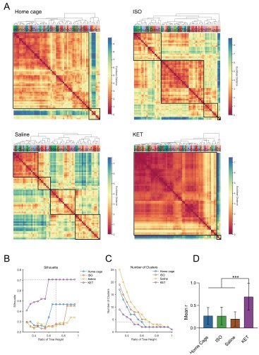
Author response image 6.
Figure 6—figure supplement 2. Hub region characterization across different conditions: home cage (A), ISO (B), saline (C), and KET (D) treatments. Brain regions are sorted by degree, betweenness centrality, and eigenvector centrality, with each metric presented in separate bar graphs. Bars to the left of the dashed line indicate the top 20% of regions by rank, highlighting the most central nodes within the network. Red bars signify regions that consistently appear within the top rankings for both degree and betweenness centrality across the metrics.
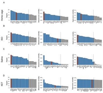
- I am still having difficulties understanding Fig. 3.
Panel A: The lack of identification for the dots in panel A makes it impossible to understand which regions are relevant.
Panel B: what is the metric that the up/down arrow summarizes? Fos density? Relative density? PC1/2?
Panel C: it's unclear to me why the regions are connected by a line. Such representation is normally used for time series/within-subject series. What is the rationale for the order of the regions?
Thank you for your patience and for reiterating your concerns regarding Figure 3.
a. In Panel A, we have substituted the original content with a display of hierarchical clustering results, which now clearly marks each brain region. This change aids readers in identifying regions with similar expression patterns and facilitates a more intuitive understanding of the data.
a. Acknowledging that our analysis did not reveal any significantly inhibited brain regions, we have decided to remove the previous version of Panel B from the figure.
b. We have discontinued the use of PCA calculations and have removed this figure to avoid any confusion it may have caused. Our revised analysis focuses on hierarchical clustering, which are presented in the updated figures.
Reviewer #2:
- Aside from issues with their data transformation (see below), (a) I think they have some interesting Fos counts data in Figures 4B and 5B that indicate shared and distinct activation patterns after KET vs. ISO based anesthesia. These data are far closer to the raw data than PC analyses and need to be described and analyzed in the first figures long before figures with the more abstracted PC analyses. In other words, you need to show the concrete raw data before describing the highly transformed and abstracted PC analyses. (b) This gets to the main point that when selecting brain areas for follow up analyses, these should be chosen based on the concrete Fos counts data, not the highly transformed and abstracted PC analyses.
Thank you for your suggestions.
a. We have added the original c-Fos cell density distribution maps for Figures 2, 3, 4, and 5 in Supplementary Figures 2 and 3 (also shown below). To maintain consistency across the document, we have updated both the y-axis label and the corresponding data in Figures 4B and 5B from 'c-Fos cell count' to 'c-Fos density'.
b. The analyses in Figures 2 and 3 include all brain regions. Figures 4 and 5 present the brain regions with significant differences as shown in Figure 3—figure supplement 1.
Author response image 7.
Figure 2—figure supplement 1. The c-Fos density in 53 brain areas for different conditions. (home cage, n = 6; ISO, n = 6 mice; saline, n = 8; KET, n = 6). Each point represents the c-Fos density in a specific brain region, denoted on the y-axis with both abbreviations and full names. Data are shown as mean ± SEM. Brain regions are categorized into 12 brain structures, as indicated on the right side of the graph.
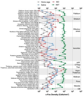
Author response image 8.
Figure 3—figure supplement 1. c-Fos density visualization across 201 distinct brain regions under various conditions. The graph depicts the c-Fos density levels for each condition, with data presented as mean and standard error. Brain regions with statistically significant differences are featured in Figures 4 and 5. Brain regions are organized into major anatomical subdivisions, as indicated on the left side of the graph.
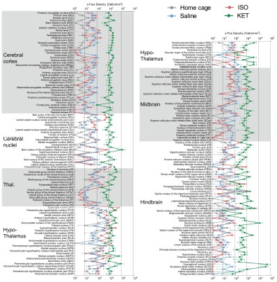
- Now, the choice of data transformation for Fos counts is the most significant problem. First, the authors show in the response letter that not using this transformation (region density/brain density) leads to no clustering. However, they also showed the region-densities without transformation (which we appreciate) and it looks like overall Fos levels in the control group Home (ISO) are a magnitude (~10-fold) higher than those in the control group Saline (KET) across all regions shown. This large difference seems unlikely to be due to a biologically driven effect and seems more likely to be due to a technical issue, such as differences in staining or imaging between experiments. Was the Homecage-ISO experiment or at least the Fos labeling and imaging performed at the same time as for the Saline-Ketamine experiment? Please state the answer to this question in the Results section one way or the other.
a. “Home (ISO) are a magnitude (~10-fold) higher than those in the control group saline (KET) across all regions shown.” We believe you might be indicating that compared to the home cage group (gray), the saline group (blue) shows a 10-fold higher expression (Supplementary Figure 2/3). Indeed, we observed that the total number of c-Fos cells in the home cage group is significantly lower than in the saline group. This difference may be due to reduced sleep during the light-on period (ZT 6- ZT 7.5) in the saline mice or the pain and stress response caused by intraperitoneal injection of saline. We have explained this discrepancy in the discussion section.Line 308-317(also see below)
“…Our findings indicate that c-Fos expression in the KET group is significantly elevated compared to the ISO group, and the saline group exhibits notably higher c-Fos expression than the home cage group, as seen in Supplementary Figures 2 and 3. Intraperitoneal saline injections in the saline group, despite pre-experiment acclimation with handling and injections for four days, may still evoke pain and stress responses in mice. Subtle yet measurable variations in brain states between the home cage and saline groups were observed, characterized by changes in normalized EEG delta/theta power (home cage: 0.05±0.09; saline: -0.03±0.11) and EMG power (home cage: -0.37±0.34; saline: 0.04±0.13), as shown in Figure 1—figure supplement 1. These changes suggest a relative increase in overall brain activity in the saline group compared to the home cage group, potentially contributing to the higher c-Fos expression…”
b. Drug administration and tissue collection for both Homecage-ISO and Saline-Ketamine groups were consistently scheduled at 13:00 and 14:30, respectively. Four mice were administered drugs and had tissues collected each day, with two from the experimental group and two from the control group, to ensure consistent sampling. The 4% PFA fixation time, sucrose dehydration time, primary and secondary antibody concentrations and incubation times, staining, and imaging parameters and equipment (exposure time for VS120 imaging was fixed at 100ms) were all conducted according to a unified protocol.
We have included the following statement in the results section: Line 81-83, “Sample collection for all mice was uniformly conducted at 14:30 (ZT7.5), and the c-Fos labeling and imaging were performed using consistent parameters throughout all experiments. ”
- Second, they need to deal with this large difference in overall staining or imaging for these two (Home/ISO and Saline/KET) experiments more directly; their current normalization choice does not really account for the large overall differences in mean values and variability in Fos counts (e.g. due to labeling and imaging differences).
3a. I think one option (not perfect but I think better than the current normalization choice) could be z-scoring each treatment to its respective control. They can analyze these z-scored data first, and then in later figures show PC analyses of these data and assess whether the two treatments separate on PC1/2. And if they don't separate, then they don't separate, and you have to go with these results.
3b. Alternatively, they need to figure out the overall intensity distributions from the different runs (if that the main reason of markedly different counts) and adjust their thresholds for Fos-positive cell detection based on this. I would expect that the saline and HC groups should have similar levels of activation, so they could use these as the 'control' group to determine a Fos-positive intensity threshold that gets applied to the corresponding 'treatment' group.
3c. If neither 3a nor 3b is an option then they need to show the outcomes of their analysis when using the untransformed data in the main figures (the untransformed data plots in their responses to reviewer are currently not in the main or supplementary figs) and discuss these as well.
a. Thank you very much for your valuable suggestion. We conducted PCA analysis on the ISO and KET data after Z-scoring them with their respective control groups and did not find any significant separation.
Author response image 9.
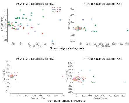
As mentioned in our response to reviewer #1, we have reprocessed the raw data. Firstly, we divided the ISO and KET data by their respective control brain regions and then performed a logarithmic transformation to obtain the log relative c-Fos density. The purpose of this is to eliminate the impact of baseline differences and reduce variability. We then performed hierarchical clustering, and finally, we Z-scored the log relative c-Fos density data. The aim is to facilitate comparison of ISO and KET on the same data dimension (Figure 2 and 3).
b. We appreciate your concerns regarding the detection thresholds for Fos-positive cells. The enclosed images, extracted from supplementary figures for Figures 4 and 5, demonstrate notable differences in c-Fos expression between saline and home cage groups in specific brain regions. These regions exhibit a discernible difference in staining intensity, with the saline group showing enhanced c-Fos expression in the PVH and PVT regions compared to the home cage group. An examination of supplementary figures for Figures 4 and 5 shows that c-Fos expression in the home cage group is consistently lower than in the saline group. This comparative analysis confirms that the discrepancies in c-Fos levels are not due to varying detection thresholds.
Author response image 10.
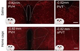
b. We have added the corresponding original data graphs to Supplementary Figures 2 and 3, and discussed the potential reasons for the significant differences between these groups in the discussion section (also shown below).
Lines 308-317: "...Our findings indicate that c-Fos expression in the KET group is significantly elevated compared to the ISO group, and the saline group exhibits notably higher c-Fos expression than the home cage group, as seen in Supplementary Figures 2 and 3. Intraperitoneal saline injections in the saline group, despite pre-experiment acclimation with handling and injections for four days, may still evoke pain and stress responses in mice. Subtle yet measurable variations in brain states between the home cage and saline groups were observed, characterized by changes in normalized EEG delta/theta power (home cage: 0.05±0.09; saline: -0.03±0.11) and EMG power (home cage: -0.37±0.34; saline: 0.04±0.13), as shown in Figure 3—figure supplement 1. These changes suggest a relative increase in overall brain activity in the saline group compared to the home cage group, potentially contributing to the higher c-Fos expression.…”
Author response:
The following is the authors’ response to the original reviews.
Responses to Reviewer’s Comments:
To Reviewer #2:
(1) The use of two m<sup>5</sup>C reader proteins is likely a reason for the high number of edits introduced by the DRAM-Seq method. Both ALYREF and YBX1 are ubiquitous proteins with multiple roles in RNA metabolism including splicing and mRNA export. It is reasonable to assume that both ALYREF and YBX1 bind to many mRNAs that do not contain m<sup>5</sup>C.
To substantiate the author's claim that ALYREF or YBX1 binds m<sup>5</sup>C-modified RNAs to an extent that would allow distinguishing its binding to non-modified RNAs from binding to m<sup>5</sup>Cmodified RNAs, it would be recommended to provide data on the affinity of these, supposedly proven, m<sup>5</sup>C readers to non-modified versus m<sup>5</sup>C-modified RNAs. To do so, this reviewer suggests performing experiments as described in Slama et al., 2020 (doi: 10.1016/j.ymeth.2018.10.020). However, using dot blots like in so many published studies to show modification of a specific antibody or protein binding, is insufficient as an argument because no antibody, nor protein, encounters nanograms to micrograms of a specific RNA identity in a cell. This issue remains a major caveat in all studies using so-called RNA modification reader proteins as bait for detecting RNA modifications in epitranscriptomics research. It becomes a pertinent problem if used as a platform for base editing similar to the work presented in this manuscript.
The authors have tried to address the point made by this reviewer. However, rather than performing an experiment with recombinant ALYREF-fusions and m<sup>5</sup>C-modified to unmodified RNA oligos for testing the enrichment factor of ALYREF in vitro, the authors resorted to citing two manuscripts. One manuscript is cited by everybody when it comes to ALYREF as m<sup>5</sup>C reader, however none of the experiments have been repeated by another laboratory. The other manuscript is reporting on YBX1 binding to m<sup>5</sup>C-containing RNA and mentions PARCLiP experiments with ALYREF, the details of which are nowhere to be found in doi: 10.1038/s41556-019-0361-y.
Furthermore, the authors have added RNA pull-down assays that should substitute for the requested experiments. Interestingly, Figure S1E shows that ALYREF binds equally well to unmodified and m<sup>5</sup>C-modified RNA oligos, which contradicts doi:10.1038/cr.2017.55, and supports the conclusion that wild-type ALYREF is not specific m<sup>5</sup>C binder. The necessity of including always an overexpression of ALYREF-mut in parallel DRAM experiments, makes the developed method better controlled but not easy to handle (expression differences of the plasmid-driven proteins etc.)
Thank you for pointing this out. First, we would like to correct our previous response: the binding ability of ALYREF to m<sup>5</sup>C-modified RNA was initially reported in doi: 10.1038/cr.2017.55, (and not in doi: 10.1038/s41556-019-0361-y), where it was observed through PAR-CLIP analysis that the K171 mutation weakens its binding affinity to m<sup>5</sup>C -modified RNA.
Our previous experimental approach was not optimal: the protein concentration in the INPUT group was too high, leading to overexposure in the experimental group. Additionally, we did not conduct a quantitative analysis of the results at that time. In response to your suggestion, we performed RNA pull-down experiments with YBX1 and ALYREF, rather than with the pan-DRAM protein, to better validate and reproduce the previously reported findings. Our quantitative analysis revealed that both ALYREF and YBX1 exhibit a stronger affinity for m<sup>5</sup>C -modified RNAs. Furthermore, mutating the key amino acids involved in m<sup>5</sup>C recognition significantly reduced the binding affinity of both readers. These results align with previous studies (doi: 10.1038/cr.2017.55 and doi: 10.1038/s41556-019-0361-y), confirming that ALYREF and YBX1 are specific readers of m<sup>5</sup>C -modified RNAs. However, our detection system has certain limitations. Despite mutating the critical amino acids, both readers retained a weak binding affinity for m<sup>5</sup>C, suggesting that while the mutation helps reduce false positives, it is still challenging to precisely map the distribution of m<sup>5</sup>C modifications. To address this, we plan to further investigate the protein structure and function to obtain a more accurate m<sup>5</sup>C sequencing of the transcriptome in future studies. Accordingly, we have updated our results and conclusions in lines 294-299 and discuss these limitations in lines 109114.
In addition, while the m<sup>5</sup>C assay can be performed using only the DRAM system alone, comparing it with the DRAM<sup>mut</sup> control enhances the accuracy of m<sup>5</sup>C region detection. To minimize the variations in transfection efficiency across experimental groups, it is recommended to use the same batch of transfections. This approach not only ensures more consistent results but also improve the standardization of the DRAM assay, as discussed in the section added on line 308-312.
(2) Using sodium arsenite treatment of cells as a means to change the m<sup>5</sup>C status of transcripts through the downregulation of the two major m<sup>5</sup>C writer proteins NSUN2 and NSUN6 is problematic and the conclusions from these experiments are not warranted. Sodium arsenite is a chemical that poisons every protein containing thiol groups. Not only do NSUN proteins contain cysteines but also the base editor fusion proteins. Arsenite will inactivate these proteins, hence the editing frequency will drop, as observed in the experiments shown in Figure 5, which the authors explain with fewer m<sup>5</sup>C sites to be detected by the fusion proteins.
The authors have not addressed the point made by this reviewer. Instead the authors state that they have not addressed that possibility. They claim that they have revised the results section, but this reviewer can only see the point raised in the conclusions. An experiment would have been to purify base editors via the HA tag and then perform some kind of binding/editing assay in vitro before and after arsenite treatment of cells.
We appreciate the reviewer’s insightful comment. We fully agree with the concern raised. In the original manuscript, our intention was to use sodium arsenite treatment to downregulate NSUN mediated m<sup>5</sup>C levels and subsequently decrease DRAM editing efficiency, with the aim of monitoring m<sup>5</sup>C dynamics through the DRAM system. However, as the reviewer pointed out, sodium arsenite may inactivate both NSUN proteins and the base editor fusion proteins, and any such inactivation would likely result in a reduced DRAM editing.
This confounds the interpretation of our experimental data.
As demonstrated in Author response image 1A, western blot analysis confirmed that sodium arsenite indeed decreased the expression of fusion proteins. In addition, we attempted in vitro fusion protein purificationusing multiple fusion tags (HIS, GST, HA, MBP) for DRAM fusion protein expression, but unfortunately, we were unable to obtain purified proteins. However, using the Promega TNT T7 Rapid Coupled In Vitro Transcription/Translation Kit, we successfully purified the DRAM protein (Author response image 1B). Despite this success, subsequent in vitro deamination experiments did not yield the expected mutation results (Author response image 1C), indicating that further optimization is required. This issue is further discussed in line 314-315.
Taken together, the above evidence supports that the experiment of sodium arsenite treatment was confusing and we determined to remove the corresponding results from the main text of the revised manuscript.
Author response image 1.
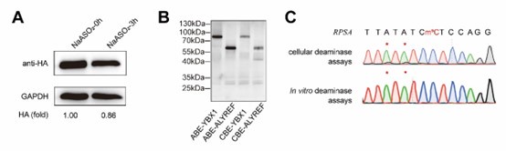
(3) The authors should move high-confidence editing site data contained in Supplementary Tables 2 and 3 into one of the main Figures to substantiate what is discussed in Figure 4A. However, the data needs to be visualized in another way then excel format. Furthermore, Supplementary Table 2 does not contain a description of the columns, while Supplementary Table 3 contains a single row with letters and numbers.
The authors have not addressed the point made by this reviewer. Figure 3F shows the screening process for DRAM-seq assays and principles for screening highconfidence genes rather than the data contained in Supplementary Tables 2 and 3 of the former version of this manuscript.
Thank you for your valuable suggestion. We have visualized the data from Supplementary Tables 2 and 3 in Figure 4A as a circlize diagram (described in lines 213-216), illustrating the distribution of mutation sites detected by the DRAM system across each chromosome. Additionally, to improve the presentation and clarity of the data, we have revised Supplementary Tables 2 and 3 by adding column descriptions, merging the DRAM-ABE and DRAM-CBE sites, and including overlapping m<sup>5</sup>C genes from previous datasets.
Responses to Reviewer’s Comments:
To Reviewer #3:
The authors have again tried to address the former concern by this reviewer who questioned the specificity of both m<sup>5</sup>C reader proteins towards modified RNA rather than unmodified RNA. The authors chose to do RNA pull down experiments which serve as a proxy for proving the specificity of ALYREF and YBX1 for m<sup>5</sup>C modified RNAs. Even though this reviewer asked for determining the enrichment factor of the reader-base editor fusion proteins (as wildtype or mutant for the identified m<sup>5</sup>C specificity motif) when presented with m<sup>5</sup>C-modified RNAs, the authors chose to use both reader proteins alone (without the fusion to an editor) as wildtype and as respective m<sup>5</sup>C-binding mutant in RNA in vitro pull-down experiments along with unmodified and m<sup>5</sup>C-modified RNA oligomers as binding substrates. The quantification of these pull-down experiments (n=2) have now been added, and are revealing that (according to SFigure 1 E and G) YBX1 enriches an RNA containing a single m<sup>5</sup>C by a factor of 1.3 over its unmodified counterpart, while ALYREF enriches by a factor of 4x. This is an acceptable approach for educated readers to question the specificity of the reader proteins, even though the quantification should be performed differently (see below).
Given that there is no specific sequence motif embedding those cytosines identified in the vicinity of the DRAM-edits (Figure 3J and K), even though it has been accepted by now that most of the m<sup>5</sup>C sites in mRNA are mediated by NSUN2 and NSUN6 proteins, which target tRNA like substrate structures with a particular sequence enrichment, one can conclude that DRAM-Seq is uncovering a huge number of false positives. This must be so not only because of the RNA bisulfite seq data that have been extensively studied by others, but also by the following calculations: Given that the m<sup>5</sup>C/C ratio in human mRNA is 0.02-0.09% (measured by mass spec) and assuming that 1/4 of the nucleotides in an average mRNA are cytosines, an mRNA of 1.000 nucleotides would contain 250 Cs. 0.02- 0.09% m<sup>5</sup>C/C would then translate into 0.05-0.225 methylated cytosines per 250 Cs in a 1000 nt mRNA. YBX1 would bind every C in such an mRNA since there is no m<sup>5</sup>C to be expected, which it could bind with 1.3 higher affinity. Even if the mRNAs would be 10.000 nt long, YBX1 would bind to half a methylated cytosine or 2.25 methylated cytosines with 1.3x higher affinity than to all the remaining cytosines (2499.5 to 2497.75 of 2.500 cytosines in 10.000 nt, respectively). These numbers indicate a 4999x to 1110x excess of cytosine over m<sup>5</sup>C in any substrate RNA, which the "reader" can bind as shown in the RNA pull-downs on unmodified RNAs. This reviewer spares the reader of this review the calculations for ALYREF specificity, which is slightly higher than YBX1. Hence, it is up to the capable reader of these calculations to follow the claim that this minor affinity difference allows the unambiguous detection of the few m<sup>5</sup>C sites in mRNA be it in the endogenous scenario of a cell or as fusion-protein with a base editor attached?
We sincerely appreciate the reviewer’s rigorous analysis. We would like to clarify that in our RNA pulldown assays, we indeed utilized the full DRAM system (reader protein fused to the base editor) to reflect the specificity of m<sup>5</sup>C recognition. As previously suggested by the reviewer, to independently validate the m<sup>5</sup>C-binding specificity of ALYREF and YBX1, we performed separate pulldown experiments with wild-type and mutant reader proteins (without the base editor fusion) using both unmodified and m<sup>5</sup>C-modified RNA substrates. This approach aligns with established methodologies in the field (doi:10.1038/cr.2017.55 and doi: 10.1038/s41556-019-0361-y). We have revised the Methods section (line 230) to explicitly describe this experimental design.
Although the m<sup>5</sup>C/C ratios in LC/MS-assayed mRNA are relatively low (ranging from 0.02% to 0.09%), as noted by the reviewer, both our data and previous studies have demonstrated that ALYREF and YBX1 preferentially bind to m<sup>5</sup>C-modified RNAs over unmodified RNAs, exhibiting 4-fold and 1.3-fold enrichment, respectively (Supplementary Figure 1E–1G). Importantly, this specificity is further enhanced in the DRAM system through two key mechanisms: first, the fusion of reader proteins to the deaminase restricts editing to regions near m<sup>5</sup>C sites, thereby minimizing off-target effects; second, background editing observed in reader-mutant or deaminase controls (e.g., DRAM<sup>mut</sup>-CBE in Figure 2D) is systematically corrected for during data analysis.
We agree that the theoretical challenge posed by the vast excess of unmodified cytosines. However, our approach includes stringent controls to alleviate this issue. Specifically, sites identified in NSUN2/NSUN6 knockout cells or reader-mutant controls are excluded (Figure 3F), which significantly reduces the number of false-positive detections. Additionally, we have observed deamination changes near high-confidence m<sup>5</sup>C methylation sites detected by RNA bisulfite sequencing, both in first-generation and high-throughput sequencing data. This observation further substantiates the validity of DRAM-Seq in accurately identifying m<sup>5</sup>C sites.
We fully acknowledge that residual false positives may persist due to the inherent limitations of reader protein specificity, as discussed in line 299-301 of our manuscript. To address this, we plan to optimize reader domains with enhanced m<sup>5</sup>C binding (e.g., through structure-guided engineering), which is also previously implemented in the discussion of the manuscript.
The reviewer supports the attempt to visualize the data. However, the usefulness of this Figure addition as a readable presentation of the data included in the supplement is up to debate.
Thank you for your kind suggestion. We understand the reviewer's concern regarding data visualization. However, due to the large volume of DRAM-seq data, it is challenging to present each mutation site and its characteristics clearly in a single figure. Therefore, we chose to categorize the data by chromosome, which not only allows for a more organized presentation of the DRAM-seq data but also facilitates comparison with other database entries. Additionally, we have updated Supplementary Tables 2 and 3 to provide comprehensive information on the mutation sites. We hope that both the reviewer and editors will understand this approach. We will, of course, continue to carefully consider the reviewer's suggestions and explore better ways to present these results in the future.
(3) A set of private Recommendations for the Authors that outline how you think the science and its presentation could be strengthened
NEW COMMENTS to TEXT:
Abstract:
"5-Methylcytosine (m<sup>5</sup>C) is one of the major post-transcriptional modifications in mRNA and is highly involved in the pathogenesis of various diseases."
In light of the increasing use of AI-based writing, and the proof that neither DeepSeek nor ChatGPT write truthfully statements if they collect metadata from scientific abstracts, this sentence is utterly misleading.
m<sup>5</sup>C is not one of the major post-transcriptional modifications in mRNA as it is only present with a m<sup>5</sup>C/C ratio of 0.02- 0.09% as measured by mass-spec. Also, if m<sup>5</sup>C is involved in the pathogenesis of various diseases, it is not through mRNA but tRNA. No single published work has shown that a single m<sup>5</sup>C on an mRNA has anything to do with disease. Every conclusion that is perpetuated by copying the false statements given in the many reviews on the subject is based on knock-out phenotypes of the involved writer proteins. This reviewer wishes that the authors would abstain from the common practice that is currently flooding any scientific field through relentless repetitions in the increasing volume of literature which perpetuate alternative facts.
We sincerely appreciate the reviewer’s insightful comments. While we acknowledge that m<sup>5</sup>C is not the most abundant post-transcriptional modification in mRNA, we believe that research into m<sup>5</sup>C modification holds considerable value. Numerous studies have highlighted its role in regulating gene expression and its potential contribution to disease progression. For example, recent publications have demonstrated that m<sup>5</sup>C modifications in mRNA can influence cancer progression, lipid metabolism, and other pathological processes (e.g., PMID: 37845385; 39013911; 39924557; 38042059; 37870216).
We fully agree with the reviewer on the importance of maintaining scientific rigor in academic writing. While m<sup>5</sup>C is not the most abundant RNA modification, we cannot simply draw a conclusion that the level of modification should be the sole criterion for assessing its biological significance. However, to avoid potential confusion, we have removed the word “major”.
COMMENTS ON FIGURE PRESENTATION:
Figure 2D:
The main text states: "DRAM-CBE induced C to U editing in the vicinity of the m<sup>5</sup>C site in AP5Z1 mRNA, with 13.6% C-to-U editing, while this effect was significantly reduced with APOBEC1 or DRAM<sup>mut</sup>-CBE (Fig.2D)." The Figure does not fit this statement. The seq trace shows a U signal of about 1/3 of that of C (about 30%), while the quantification shows 20+ percent
Thank you for your kind suggestion. Upon visual evaluation, the sequencing trace in the figure appears to suggest a mutation rate closer to 30% rather than 22%. However, relying solely on the visual interpretation of sequencing peaks is not a rigorous approach. The trace on the left represents the visualization of Sanger sequencing results using SnapGene, while the quantification on the right is derived from EditR 1.0.10 software analysis of three independent biological replicates. The C-to-U mutation rates calculated were 22.91667%, 23.23232%, and 21.05263%, respectively. To further validate this, we have included the original EditR analysis of the Sanger sequencing results for the DRAM-CBE group used in the left panel of Figure 2D (see Author response image 2). This analysis confirms an m<sup>5</sup>C fraction (%) of 22/(22+74) = 22.91667, and the sequencing trace aligns well with the mutation rate we reported in Figure 2D. In conclusion, the data and conclusions presented in Figure 2D are consistent and supported by the quantitative analysis.
Author response image 2.
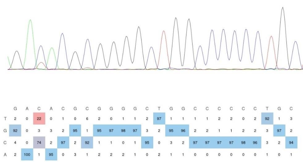
Figure 4B: shows now different numbers in Venn-diagrams than in the same depiction, formerly Figure 4A
We sincerely thank the reviewer for pointing out this issue, and we apologize for not clearly indicating the changes in the previous version of the manuscript. In response to the initial round of reviewer comments, we implemented a more stringent data filtering process (as described in Figure 3F and method section) : "For high-confidence filtering, we further adjusted the parameters of Find_edit_site.pl to include an edit ratio of 10%–60%, a requirement that the edit ratio in control samples be at least 2-fold higher than in NSUN2 or NSUN6knockout samples, and at least 4 editing events at a given site." As a result, we made minor adjustments to the Venn diagram data in Figure 4A, reducing the total number of DRAM-edited mRNAs from 11,977 to 10,835. These changes were consistently applied throughout the manuscript, and the modifications have been highlighted for clarity. Importantly, these adjustments do not affect any of the conclusions presented in the manuscript.
Figure 4B and D: while the overlap of the DRAM-Seq data with RNA bisulfite data might be 80% or 92%, it is obvious that the remaining data DRAM seq suggests a detection of additional sites of around 97% or 81.83%. It would be advised to mention this large number of additional sites as potential false positives, unless these data were normalized to the sites that can be allocated to NSUN2 and NSUN6 activity (NSUN mutant data sets could be substracted).
Thank you for pointing this out. The Venn diagrams presented in Figure 4B and D already reflect the exclusion of potential false-positive sites identified in methyltransferasedeficient datasets, as described in our experimental filtering process, and they represent the remaining sites after this stringent filtering. However, we acknowledge that YBX1 and ALYREF, while preferentially binding to m<sup>5</sup>C-modified RNA, also exhibit some affinity for unmodified RNA. Although we employed rigorous controls, including DRAM<sup>mut</sup> and deaminase groups, to minimize false positives, the possibility of residual false positives cannot be entirely ruled out. Addressing this limitation would require even more stringent filtering methods, as discussed in lines 299–301 of the manuscript. We are committed to further optimizing the DRAM system to enhance the accuracy of transcriptome-wide m<sup>5</sup>C analysis in future studies.
SFigure 1: It is clear that the wild type version of both reader proteins are robustly binding to RNA that does not contain m<sup>5</sup>C. As for the calculations of x-fold affinity loss of RNA binding using both ALYREF -mut or YBX1 -mut, this reviewer asks the authors to determine how much less the mutated versions of the proteins bind to a m<sup>5</sup>C-modified RNAs. Hence, a comparison of YBX1 versus YBX1 -mut (ALYREF versus ALYREF -mut) on the same substrate RNA with the same m<sup>5</sup>C-modified position would allow determining the contribution of the so-called modification binding pocket in the respective proteins to their RNA binding. The way the authors chose to show the data presently is misleading because what is compared is the binding of either the wild type or the mutant protein to different RNAs.
We appreciate the reviewer’s valuable feedback and apologize for any confusion caused by the presentation of our data. We would like to clarify the rationale behind our approach. The decision to present the wild-type and mutant reader proteins in separate panels, rather than together, was made in response to comments from Reviewer 2. Below, we provide a detailed explanation of our experimental design and its justification.
First, we confirmed that YBX1 and ALYREF exhibit stronger binding affinity to m<sup>5</sup>Cmodified RNA compared to unmodified RNA, establishing their role as m<sup>5</sup>C reader proteins. Next, to validate the functional significance of the DRAM<sup>mut</sup> group, we demonstrated that mutating key amino acids in the m<sup>5</sup>C-binding pocket significantly reduces the binding affinity of YBX1<sup>mut</sup> and ALYREF<sup>mut</sup> to m<sup>5</sup>C-modified RNA. This confirms that the DRAM<sup>mut</sup> group effectively minimizes false-positive results by disrupting specific m<sup>5</sup>C interactions.
Crucially, in our pull-down experiments, both the wild-type and mutant proteins (YBX1/YBX1<sup>mut</sup> and ALYREF/ALYREF<sup>mut</sup>) were incubated with the same RNA sequences. To avoid any ambiguity, we have included the specific RNA sequence information in the Methods section (lines 463–468). This ensures a assessment of the reduced binding affinity of the mutant versions relative to the wild-type proteins, even though they are presented in separate panels.
We hope this explanation clarifies our approach and demonstrates the robustness of our findings. We sincerely appreciate the reviewer’s understanding and hope this addresses their concerns.
SFigure 2C: first two panels are duplicates of the same image.
Thank you for pointing this out. We sincerely apologize for incorrectly duplicating the images. We have now updated Supplementary Figure 2C with the correct panels and have provided the original flow cytometry data for the first two images. It is important to note that, as demonstrated by the original data analysis, the EGFP-positive quantification values (59.78% and 59.74%) remain accurate. Therefore, this correction does not affect the conclusions of our study. Thank you again for bringing this to our attention.
Author response image 3.
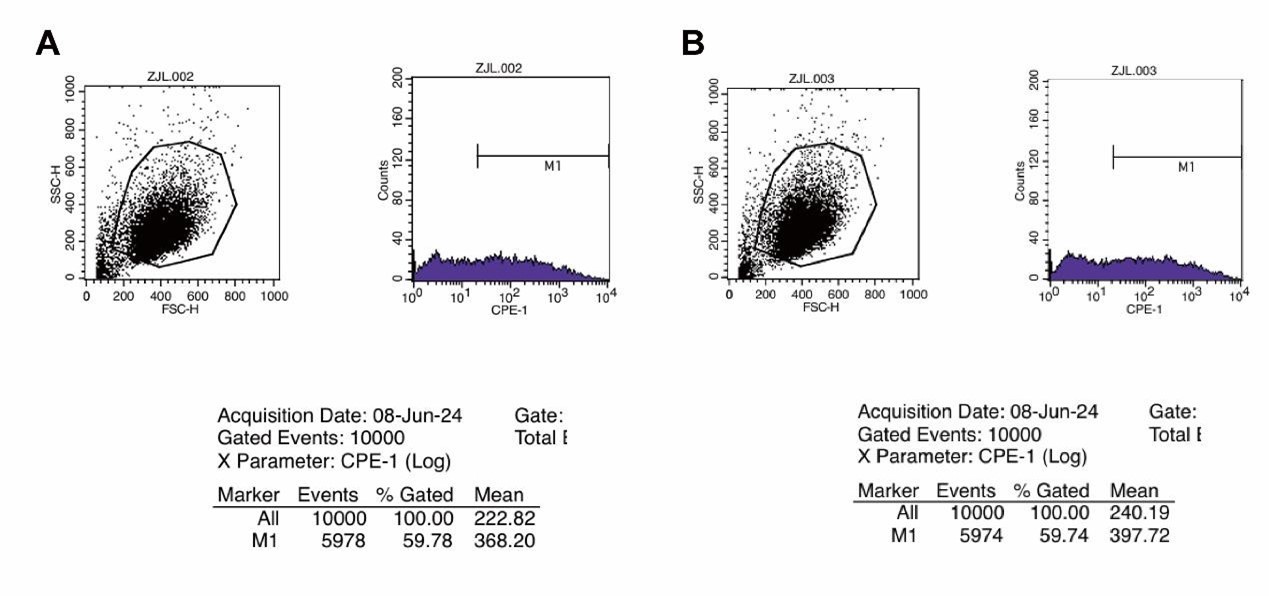
SFigure 4B: how would the PCR product for NSUN6 be indicative of a mutation? The used primers seem to amplify the wildtype sequence.
Thank you for your kind suggestion. In our NSUN6<sup>-/-</sup> cell line, the NSUN6 gene is only missing a single base pair (1bp) compared to the wildtype, which results in frame shift mutation and reduction in NSUN6 protein expression. We fully agree with the reviewer that the current PCR gel electrophoresis does not provide a clear distinction of this 1bp mutation. To better illustrate our experimental design, we have included a schematic representation of the knockout sequence in SFigure 4B. Additionally, we have provided the original sequencing data, and the corresponding details have been added to lines 151-153 of the manuscript for further clarification.
Author response image 4.
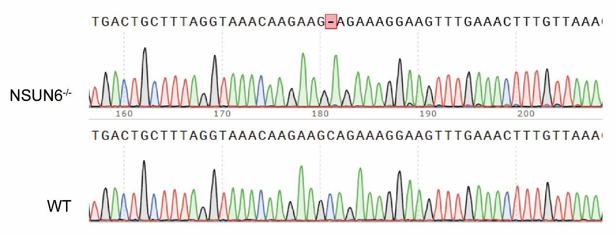
SFigure 4C: the Figure legend is insufficient to understand the subfigure.
Thank you for your valuable suggestion. To improve clarity, we have revised the figure legend for SFigure 4C, as well as the corresponding text in lines 178-179. We have additionally updated the title of SFigure 4 for better clarity. The updated SFigure 4C now demonstrates that the DRAM-edited mRNAs exhibit a high degree of overlap across the three biological replicates.
SFigure 4D: the Figure legend is insufficient to understand the subfigure.
Thank you for your kind suggestion. We have revised the figure legend to provide a clearer explanation of the subfigure. Specifically, this figure illustrates the motif analysis derived from sequences spanning 10 nucleotides upstream and downstream of DRAMedited sites mediated by loci associated with NSUN2 or NSUN6. To enhance clarity, we have also rephrased the relevant results section (lines 169-175) and the corresponding discussion (lines 304-307).
SFigure 7: There is something off with all 6 panels. This reviewer can find data points in each panel that do not show up on the other two panels even though this is a pairwise comparison of three data sets (file was sent to the Editor) Available at https://elife-rp.msubmit.net/elife-rp_files/2025/01/22/00130809/02/130809_2_attach_27_15153.pdf
Response: We thank the reviewer for pointing this out. We would like to clarify the methodology behind this analysis. In this study, we conducted pairwise comparisons of the number of DRAM-edited sites per gene across three biological replicates of DRAM-ABE or DRAM-CBE, visualized as scatterplots. Each data point in the plots corresponds to a gene, and while the same gene is represented in all three panels, its position may vary vertically or horizontally across the panels. This variation arises because the number of mutation sites typically differs between replicates, making it unlikely for a data point to occupy the exact same position in all panels. A similar analytical approach has been used in previous studies on m6A (PMID: 31548708). To address the reviewer’s concern, we have annotated the corresponding positions of the questioned data points with arrows in Author response image 5.
Author response image 5.
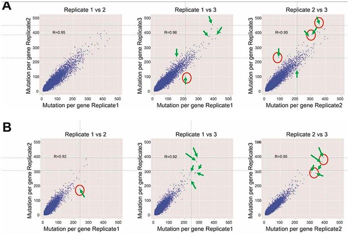
Author response:
The following is the authors’ response to the previous reviews
Public Reviews:
Reviewer #1 (Public review):
The authors investigated the role of the C. elegans Flower protein, FLWR-1, in synaptic transmission, vesicle recycling, and neuronal excitability. They confirmed that FLWR-1 localizes to synaptic vesicles and the plasma membrane and facilitates synaptic vesicle recycling at neuromuscular junctions. They observed that hyperstimulation results in endosome accumulation in flwr-1 mutant synapses, suggesting that FLWR-1 facilitates the breakdown of endocytic endosomes. Using tissue-specific rescue experiments, the authors showed that expressing FLWR-1 in GABAergic neurons restored the aldicarb-resistant phenotype of flwr-1 mutants to wild-type levels. By contrast, cholinergic neuron expression did not rescue aldicarb sensitivity at all. They also showed that FLWR-1 removal leads to increased Ca<sup>2+</sup> signaling in motor neurons upon photo-stimulation. From these findings, the authors conclude that FLWR-1 helps maintain the balance between excitation and inhibition (E/I) by preferentially regulating GABAergic neuronal excitability in a cell-autonomous manner.
Overall, the work presents solid data and interesting findings, however the proposed cell-autonomous model of GABAergic FLWR-1 function may be overly simplified in my opinion.
Most of my previous comments have been addressed; however, two issues remain.
(1) I appreciate the authors' efforts conducting additional aldicarb sensitivity assays that combine muscle-specific rescue with either cholinergic or GABergic neuron-specific expression of FLWR-1. In the revised manuscript, they conclude, "This did not show any additive effects to the pure neuronal rescues, thus FLWR-1 effects on muscle cell responses to cholinergic agonists must be cellautonomous." However, I find this interpretation confusing for the reasons outlined below.
Figure 1 - Figure Supplement 3B shows that muscle-specific FLWR-1 expression in flwr-1 mutants significantly restores aldicarb sensitivity. However, when FLWR-1 is co-expressed in both cholinergic neurons and muscle, the worms behave like flwr-1 mutants and no rescue is observed. Similarly, cholinergic FLWR-1 alone fails to restore aldicarb sensitivity (shown in the previous manuscript).
This data is still shown in the manuscript, Fig. 3D. We interpreted our finding in the muscle/cholinergic co-rescue experiment as meaning, that FLWR-1 in cholinergic neurons over-compensates, so worms should be resistant, and the rescuing effect of muscle FLWR-1 is therefore cancelled. But it is true, if this were the case, why does the pure cholinergic rescue not show over-compensation? We added a sentence to acknowledge this inconsistency and we added a sentence in the discussion (see also below, comment 1) of reviewer #2).
These observations indicate a non-cell-autonomous interaction between cholinergic neurons and muscle, rather than a strictly muscle cell-autonomous mechanism. In other words, FLWR-1 expressed in cholinergic neurons appears to negate or block the rescue effect of muscle-expressed FLWR-1. Therefore, FLWR-1 could play a more complex role in coordinating physiology across different tissues. This complexity may affect interpretations of Ca<sup>2+</sup> dynamics and/or functional data, particularly in relation to E/I balance, and thus warrants careful discussion or further investigation.
For the Ca<sup>2+</sup> dynamics, we think the effects of flwr-1 are likely very immediate, as the imaging assay relies on a sensor expressed directly in the neurons or muscles under study, and not on indirect phenotypes as muscle contraction and behavior, that depend on an interplay of several cell types influencing each other.
(2) The revised manuscript includes new GCaMP analyses restricted to synaptic puncta. The authors mention that "we compared Ca<sup>2+</sup> signals in synaptic puncta versus axon shafts, and did not find any differences," concluding that "FLWR-1's impact is local, in synaptic boutons." This is puzzling: the similarity of Ca<sup>2+</sup> signals in synaptic regions and axon shafts seems to indicate a more global effect on Ca<sup>2+</sup> dynamics or may simply reflect limited temporal resolution in distinguishing local from global signals due to rapid Ca<sup>2+</sup> diffusion. The authors should clarify how they reached the conclusion that FLWR-1 has a localized impact at synaptic boutons, given that synaptic and axonal signals appear similar. Based on the presented data, the evidence supporting a local effect of FLWR-1 on Ca<sup>2+</sup> dynamics appears limited.
We apologize, here we simply overlooked this misleading wording in our rebuttal letter. The data we mentioned, showing no obvious difference in axon vs. bouton, are shown below, including time constants for the onset and the offset of the stimulus (data is peak normalized for better visualization):
Author response image 1.
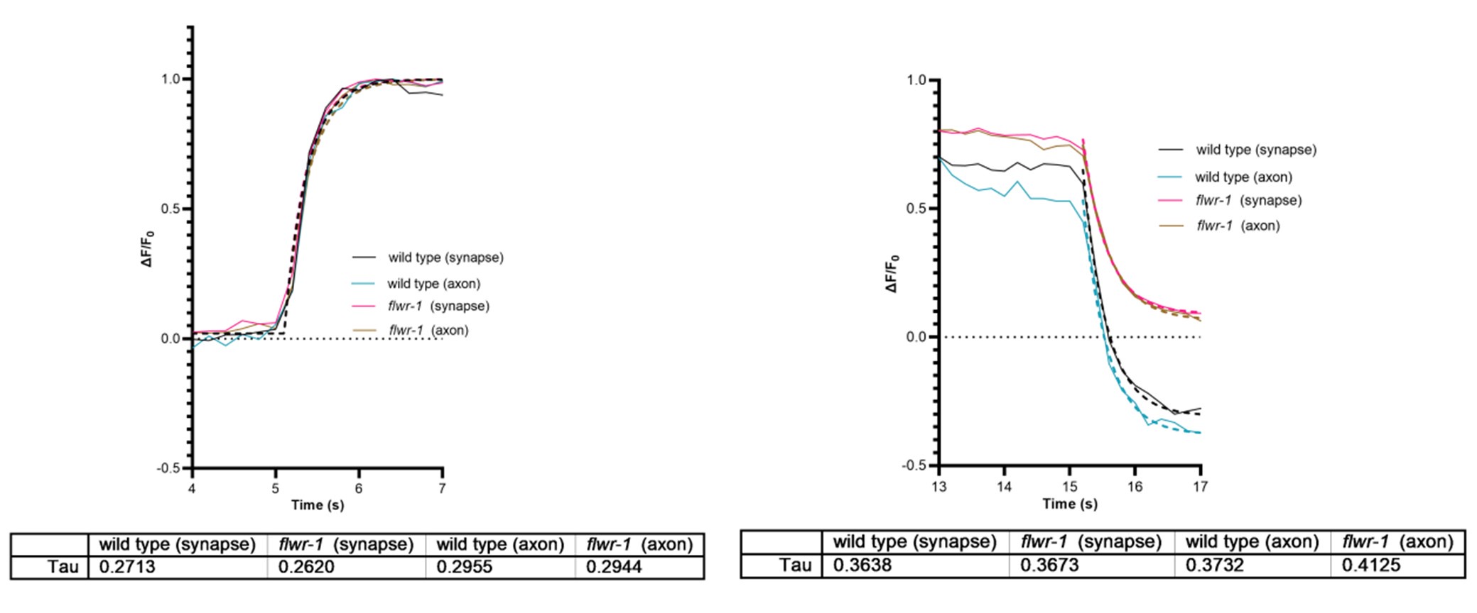
One can see that axonal Ca<sup>2+</sup> signals may rise a bit slower than synaptic Ca<sup>2+</sup> signals, as expected for Ca<sup>2+</sup> entering the boutons, and then diffusing out into the axon. The loss of FLWR1 does not affect this. However, the temporal resolution of the used GCaMP6f sensor is ca. 200 ms to reach peak, and the decay time (to t1/2) is ca. 400 ms (PMID: 23868258). Thus, it would be difficult to see effects based on Ca<sup>2+</sup> diffusion using this assay. For the decay, this is similar for both axon and synapse, while flwr-1 mutants do not reduce Ca<sup>2+</sup> as much as wt. In the axon, there is a seemingly slightly slower reduction in flwr-1 mutants, however, given the kinetics of the sensor, this is likely not a meaningful difference. Therefore, we wrote we did not find differences. The interpretation should not have been that the impact of FLWR-1 is local. It may be true if one could image this at faster time scales, i.e. if there is more FLWR-1 localized in boutons (as indicated by our data showing FLWR-1 enrichment in boutons; Fig. 3), and when considering its possible effect on MCA-3 localization (and assuming that MCA-3 is the active player in Ca<sup>2+</sup> removal), i.e. FLWR-1 recruiting MCA-3 to boutons (Fig. 9C, D).
Reviewer #2 (Public review):
Summary:
The Flower protein is expressed in various cell types, including neurons. Previous studies in flies have proposed that Flower plays a role in neuronal endocytosis by functioning as a Ca<sup>2+</sup> channel. However, its precise physiological roles and molecular mechanisms in neurons remain largely unclear. This study employs C. elegans as a model to explore the function and mechanism of FLWR-1, the C. elegans homolog of Flower. This study offers intriguing observations that could potentially challenge or expand our current understanding of the Flower protein. Nevertheless, further clarification or additional experiments are required to substantiate the study's conclusions.
Strengths:
A range of approaches was employed, including the use of a flwr-1 knockout strain, assessment of cholinergic synaptic activity via analyzing aldicarb (a cholinesterase inhibitor) sensitivity, imaging Ca<sup>2+</sup> dynamics with GCaMP3, analyzing pHluorin fluorescence, examination of presynaptic ultrastructure by EM, and recording postsynaptic currents at the neuromuscular junction. The findings include notable observations on the effects of flwr-1 knockout, such as increased Ca<sup>2+</sup> levels in motor neurons, changes in endosome numbers in motor neurons, altered aldicarb sensitivity, and potential involvement of a Ca<sup>2+</sup>-ATPase and PIP2 binding in FLWR-1's function.
The authors have adequately addressed most of my previous concerns, however, I recommend minor revisions to further strengthen the study's rigor and interpretation:
Major suggestions
(1) This study relies heavily on aldicarb assays to support its conclusions. While these assays are valuable, their results may not fully align with direct assessment of neurotransmitter release from motor neurons. For instance, prior work has shown that two presynaptic modulators identified through aldicarb sensitivity assays exhibited no corresponding electrophysiological defects at the neuromuscular junction (Liu et al., J Neurosci 27: 10404-10413, 2007). Similarly, at least one study from the Kaplan lab has noted discrepancies between aldicarb assays and electrophysiological analyses. The authors should consider adding a few sentences in the Discussion to acknowledge this limitation and the potential caveats of using aldicarb assays, especially since some of the aldicarb assay results in this study are not easily interpretable.
Aldicarb assays have been used very successfully in identifying mutants with defects in chemical synaptic transmission, and entire genetic screens have been conducted this way. The reviewer is right, one needs to realize that it is the balance of excitation and inhibition at the NMJ of C. elegans, which underlies the effects on the rate of aldicarb-induced paralysis, not just cholinergic transmission. I.e. if a given mutant affects cholinergic and GABAergic transmission differently, things become difficult to interpret, particularly if also muscle physiology is affected. Therefore, we combined mutant analyses with cell-type specific rescue. We acknowledge that results are nonetheless difficult to interpret. We thus added a sentence in the first paragraph of the discussion.
(2) The manuscript states, "Elevated Ca<sup>2+</sup> levels were not further enhanced in a flwr-1;mca-3 double mutant." (lines 549-550). However, Figure 7C does not include statistical comparisons between the single and double mutants of flwr-1 and mca-3. Please add the necessary statistical analysis to support this statement.
Because we only marked significant differences in that figure, and n.s. was not shown. This was stated in the figure legend.
(3) The term "Ca<sup>2+</sup> influx" should be avoided, as this study does not provide direct evidence (e.g. voltage-clamp recordings of Ca<sup>2+</sup> inward currents in motor neurons) for an effect of the flwr-1 mutation of Ca<sup>2+</sup> influx. The observed increase in neuronal GCaMP signals in response to optogenetic activation of ChR2 may result from, or be influenced by, Ca<sup>2+</sup> mobilization from of intracellular stores. For example, optogenetic stimulation could trigger ryanodine receptor-mediated Ca<sup>2+</sup> release from the ER via calcium-induced calcium release (CICR) or depolarization-induced calcium release (DICR). It would be more appropriate to describe the observed increase in Ca<sup>2+</sup> signal as "Ca<sup>2+</sup> elevation" rather than increased "Ca<sup>2+</sup> influx".
Ok, yes, we can do this, we referred by ‘influx’ to cytosolic Ca<sup>2+</sup>, that fluxes into the cytosol, be it from the internal stores or the extracellular. Extracellular influx, more or less, inevitably will trigger further influx from internal stores, to our understanding. We changed this to “elevated Ca<sup>2+</sup> levels” or “Ca<sup>2+</sup> level rise” or “Ca<sup>2+</sup> level increase”.
Recommendations for the authors:
Reviewer #1 (Recommendations for the authors):
A thorough discussion on the impact of cell-autonomous versus non-cell-autonomous effects is necessary.
Revise and clarify the distinction between local and global Ca²⁺ changes.
see above.
Reviewer #2 (Recommendations for the authors):
Minor suggestions
(1) In "Few-Ubi was shown to facilitate recovery of neurons following intense synaptic activity (Yao et al.,....." (lines 283-284), please specify which aspects of neuronal recovery are influenced by the Flower protein.
We added “refilling of SV pools”.
(2) The abbreviation "Few-Ubi" is used for the Drosophila Flower protein (e.g., line 283, Figure 1A, and Figure 8A). Please clarify what "Ubi" stands for and verify whether its inclusion in the protein name is appropriate.
This is inconsistent across the literature, sometimes Fwe-Ubi is also referred to as FweA. We now added this term. Ubi refers to ubiquitous (“Therefore, we named this isoform fweubi because it is expressed ubiquitously in imaginal discs“) (Rhiner 2010)
(3) The manuscript uses "pflwr-1" (line 303 and elsewhere) to denote the flwr-1 promoter. This notation could be misleading, as it may be interpreted as a gene name. Please consider using either "flwr-1p" or "Pflwr-1" instead. Additionally, ensure proper italicization of gene names throughout the manuscript.
We changed this throughout. We will change to italicized at proof stage, it would be too timeconsuming to spot these incidents now.
(4) The authors tagged the C-terminus of FLWR-1 by GFP (lines 321). The fusion protein is referred to as "GFP::FLWR-1" throughout the manuscript. Please verify whether "FLWR-1::GFP" would be the more appropriate designation.
Thank you, yes, we changed this in the text, GFP is indeed N-terminal.
(5) In "This did not show any additive effects...." (line 363), please clarify what "This" refers to.
Altered to “The combined rescues did not show any additive effects…”
(6) In "..., supporting our previous finding of increased neurotransmitter release in GABAergic neurons" (lines 412-413), please provide a citation for the referenced previous study.
This refers to our aldicarb data within this paper, just further up in the text. We removed “previous”.
(7) Figure 4C, D examines the effect of flwr-1 mutation on body length in the genetic background of the unc-29 mutation, which selectively disrupts the levamisole-sensitive acetylcholine receptor. Please comment on the rationale for implicating only the levamisole receptor rather than the nicotinic acetylcholine receptor in muscle cells.
This was because we used a behavioral assay. Despite the fact that the homopentameric ACR16/N-AChR mediate about 2/3 of the peak currents in response to acute ACh application to the NMJ (e.g. Almedom et al., EMBO J, 2009), the acr-16 mutant has virtually no behavioral / locomotion phenotype. Likely, this is because the heteropentameric, UNC-29 containing LAChR, while only contributing 1/3 of the peak current, desensitizes much more slowly and thus unc-29 mutants show a severe behavioral phenotype (uncoordinated locomotion, etc.). We thus did not expect a major effect when performing the behavoral assay in acr-16 mutants and thus chose the unc-29 mutant background.
(8) In "we found no evidence ....insertion into the PM (Yao et al., 2009)", It appears that the cited paper was not authored by any of the current manuscript. Please confirm whether this citation is correctly attributed.
This sentence was arranged in a misleading way, we did not mean that we authored this paper. It was change in the text: “While a facilitating role of Flower in endocytosis appears to be conserved in C. elegans, in contrast to previous findings from Drosophila (Yao et al., 2009), we found no evidence that FLWR-1 conducts Ca<sup>2+</sup> upon insertion into the PM.”
Author response:
The following is the authors’ response to the previous reviews
Reviewer #1 (Public review):
Summary:
This study examines to what extent this phenomenon varies based on the visibility of the saccade target. Visibility is defined as the contrast level of the target with respect to the noise background, and it is related to the signal-to-noise ratio of the target. A more visible target facilitates the oculomotor behavior planning and execution, however, as speculated by the authors, it can also benefit foveal prediction even if the foveal stimulus visibility is maintained constant. Remarkably, the authors show that presenting a highly visible saccade target is beneficial for foveal vision as detection of stimuli with an orientation similar to that of the saccade target is improved, the lower is the saccade target visibility, the less prominent is this effect.
Strengths:
The results are convincing and the research methodology is technically sound.
Weaknesses:
It is still unclear why the pre-saccadic enhancement would oscillate for targets with higher opacity levels, and what would be the benefit of this oscillatory pattern. The authors do not speculate too much on this and loosely relate it to feedback processes, which are characterized by neural oscillations in a similar range.
We thank the reviewer for their assessment. We intentionally decided to describe the oscillatory pattern without claiming to be able to pinpoint its origin. The finding was incidental and, based on psychophysical data alone, we would not feel comfortable doing anything but loosely relating it to potential mechanisms on an explicitly speculative basis. In the potential explanation we provide in the manuscript, the oscillatory pattern would likely not serve a benefit–rather, it would constitute an innate consequence and, thus, a coincidental perceptual signature of potential feedback processes.
Reviewer #2 (Public review):
Summary:
In this manuscript, the authors ran a dual task. Subjects monitored a peripheral location for a target onset (to generate a saccade to), and they also monitored a foveal location for a foveal probe. The foveal probe could be congruent or incongruent with the orientation of the peripheral target. In this study, the authors manipulated the conspicuity of the peripheral target, and they saw changes in performance in the foveal task. However, the changes were somewhat counterintuitive.
We regret that our findings remain counterintuitive to the reviewer even after our extensive explanations in the previous revision round and the corresponding changes in the manuscript. We repeat that both the decrease in foveal Hit Rates and the increase in foveal enhancement with increasing target contrast were expected and preregistered prior to data collection.
Strengths:
The authors use solid analysis methods and careful experimental design.
Comments on revisions:
The authors have addressed my previous comments.
One minor thing is that I am confused by their assertion that there was no smoothing in the manuscript (other than the newly added time course analysis). Figure 3A and Figure 6 seem to have smoothing to me.
When the reviewer suggested that the “data appear too excessively smoothed” in the first revision, we assumed that they were referring to pre-saccadic foveal Hit and False Alarm rates, not to fitted distributions. As we state in the legend of Figure 3A (as well as in Figures 6 and S1), the “smoothed” curves constitute the probability density distributions of our raw data. Concerning the energy maps resulting from reverse correlation analyses, we described our proceeding in detail in our initial article (Kroell & Rolfs, 2022):
“Using this method, we obtained filter responses for 260 SF*ori combinations per noise image (Figure 6 in Materials and methods, ‘Stimulus analysis’). SFs ranged from 0.33 to 1.39 cpd (in 20 equal increments). Orientations ranged from –90–90° (in 13 equal increments). To normalize the resulting energy maps, we z-transformed filter responses using the mean and standard deviation of filter responses from the set of images presented in a certain session. To obtain more fine-grained maps, we applied 2D linear interpolations by iteratively halving the interval between adjacent values 4 times in each dimension. To facilitate interpretability, we flipped the energy maps of trials in which the target was oriented to the left. In all analyses and plots,+45° thus corresponds to the target’s orientation while –45° corresponds to the other potential probe orientation. Filter responses for all response types are provided at https://osf.io/v9gsq/.”
We have added a pointer to this explanation to the current manuscript (see line 836).
Another minor comment is related to the comment of Reviewer 1 about oscillations. Another possible reason for what looks like oscillations is saccadic inhibition. when the foveal probe appears, it can reset the saccade generation process. when aligned to saccade onset, this appears like a characteristic change in different parameters that is time-locked to saccade onset (about a 100 ms earlier). So, maybe the apparent oscillation is a manifestation of such resetting and it's not really an oscillation. so, I agree with Reviewer 1 about removing the oscillation sentence from the abstract.
While we understand that a visible probe will result in saccadic inhibition (White & Rolfs, 2016), we are unsure how a resetting of the saccade generation process should manifest in increased perceptual enhancement of a specific, peripheral target orientation in the presaccadic fovea. Moreover, as we describe in our initial article (Kroell & Rolfs, 2022), we updated the background noise image every 50 ms and embedded our probe stimulus into the surrounding noise using smooth orientation filters and raised cosine masks to avoid a disruptive influence of probe appearance on movement planning and execution (Hanning, Deubel, & Szinte, 2019). And indeed, we demonstrated that the appearance of the foveal probe did not disrupt saccade preparation, that is, did not increase saccade latencies compared to ‘probe absent’ trials in which no foveal probe was presented (see Kroell & Rolfs, 2022; sections “Parameters of included saccades in Experiment 1” and “Parameters of included saccades in Experiment 2”). In the current submission, saccade latencies in ‘probe present’ trials exceeded saccade latencies in ‘probe absent’ trials by a mere 4.7±2.3 ms. Additionally, to inspect the variation of saccade execution frequency directly, we aligned the number of saccade generation instances to the onset of the foveal probe stimulus (see Author response image 1). In line with what we described in a previous paradigm employing flickering bandpass filtered noise patches (Kroell & Rolfs, 2021; 10.1016/j.cortex.2021.02.021), we observed a regular variation in saccade execution frequency that reflected the duration of an individual background noise image (50 ms in this investigation). In other words, the repeated dips in saccadic frequency are likely caused by the flickering background noise and not the onset of the foveal probe which would produce a single dip ~100 ms after probe onset. Given these results, we do not see a straight-forward explanation for how the variation of saccade execution frequency in 20 Hz intervals would boost peripheral-to-foveal feature prediction before the saccade in ~10 Hz intervals. Nonetheless, we removed the sentence referencing oscillations from the Abstract.
Author response image 1.
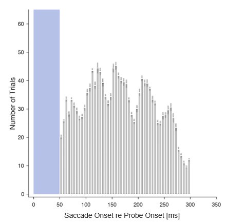
Recommendations for the authors:
Reviewer #1 (Recommendations for the authors):
Overall, The authors did a good job in addressing the points I raised. Two new sections were added to the manuscript, one to address how the mechanisms of foveal predictions would play out in natural viewing conditions, and another one examining more in depth the potential neural mechanisms implicated in foveal predictions. I found these two sections to be quite speculative, and at points, a bit convoluted but could help the reader get the bigger picture. I still do not have a clear sense of why the pre-saccadic enhancement would oscillate for targets with higher opacity levels, and what would be the benefit of this oscillatory pattern. The authors do not speculate too much on this and loosely relate it to feedback processes, which are characterized by neural oscillations in a similar range.
Please see our response to ‘Weaknesses’.
I still find this a loose connection and would suggest removing the following phrase from the abstract "Interestingly, the temporal frequency of these oscillations corresponded to the frequency range typically associated with neural feedback signaling".
We have removed this phrase.
Finally, the authors should specify how much of this oscillation is due to oscillations in HR of cong vs. oscillations in HR of incongruent trials or both.
We fitted separate polynomials to congruent and incongruent Hit Rates instead of their difference. Peaks in enhancement relied on both, oscillatory increases in congruent Hit Rates and simultaneous decreases in incongruent Hit Rates. In other words, enhancement peaks appear to reflect a foveal enhancement of target-congruent feature information along with a concurrent suppression of target-incongruent features. We added this paragraph and Figure 4 to the Results section.
Additional changes:
Two figures had accidentally been labeled as Figure 5 in our first revision. We corrected the figure legends and all corresponding figure references in the text.
Author response:
The following is the authors’ response to the previous reviews.
As to the exceptionally minor issue, namely, correction for multiple statistical tests (minor because the data and the error are presented in the text). We have now conducted one-way ANOVA to back the data displayed in Fig 4A., and Supp. Figs 19 and 21. In each case ANOVA revealed a highly significant difference among means: Dunnett’s post hoc test was then used to test each result against SBW25, with the multiple comparisons corrected for in the analysis.
This resulted in changes to the description of the statistical analysis in the following captions:
To Figure 4.
Where we previously referred to paired t-tests we now state: ANOVA revealed a highly significant difference among means [F<sub>7,16</sub> = 8.19, p < 0.001] with Dunnett’s post-hoc test adjusted for multiple comparisons showing that five genotypes (*) differ significantly (p < 0.05) from SBW25.
To Supplementary Figure 19.
Where we previously referred to paired t-tests we now state: ANOVA revealed a highly significant difference among means [F<sub>7,16</sub> = 16.74, p < 0.001] with Dunnett’s post-hoc test adjusted for multiple comparisons showing that three genotypes (*) differ significantly (p < 0.05) from SBW25.
To Supplementary Figure 21.
Where we previously referred to paired t-tests we now state: ANOVA revealed a highly significant difference among means [F<sub>7,89</sub> = 9.97, p < 0.0001] with Dunnett’s post-hoc test adjusted for multiple comparisons showing that SBW25 ∆mreB and SBW25 ∆PFLU4921-4925 are significantly different (*) from SBW25 (p < 0.05).
The following is the authors’ response to the original reviews.
Public Reviews:
Reviewer #1 (Public Review):
Summary:
The authors performed experimental evolution of MreB mutants that have a slow-growing round phenotype and studied the subsequent evolutionary trajectory using analysis tools from molecular biology. It was remarkable and interesting that they found that the original phenotype was not restored (most common in these studies) but that the round phenotype was maintained.
Strengths:
The finding that the round phenotype was maintained during evolution rather than that the original phenotype, rod-shaped cells, was recovered is interesting. The paper extensively investigates what happens during adaptation with various different techniques. Also, the extensive discussion of the findings at the end of the paper is well thought through and insighXul.
Weaknesses:
I find there are three general weaknesses:
(1) Although the paper states in the abstract that it emphasizes "new knowledge to be gained" it remains unclear what this concretely is. On page 4 they state 3 three research questions, these could be more extensively discussed in the abstract. Also, these questions read more like genetics questions while the paper is a lot about cell biological findings.
Thank you for drawing attention to the unnecessary and gratuitous nature of the last sentence of the Abstract. We are in agreement. It has been modified, and we have taken advantage of additional word space to draw attention to the importance of the two competing (testable) hypotheses laid out in the Discussion.
As to new knowledge, please see the Results and particularly the Discussion. But beyond this, and as recognised by others, there is real value for cell biology in seeing how (and whether) selection can compensate for effects that are deleterious to fitness. The results will very often depart from those delivered from, for example, suppressor analyses, or bottom up engineering.
In the work recounted in our paper, we chose to focus – by way of proof-of principle – on the most commonly observed mutations, namely, those within pbp1A. But beyond this gene, we detected mutations in other components of the cell shape / division machinery whose connections are not yet understood and which are the focus of on-going investigation.
As to the three questions posed at the end of the Introduction, the first concerns whether selection can compensate for deleterious effects of deleting mreB (a question that pertains to evolutionary aspects); the second seeks understanding of genetic factors; the third aims to shed light on the genotype-to-phenotype map (which is where the cell biology comes into play). Given space restrictions, we cannot see how we could usefully expand, let alone discuss, the three questions raised at the end of the Introduction in restrictive space available in the Abstract.
(2) It is not clear to me from the text what we already know about the restoration of MreB loss from suppressors studies (in the literature). Are there suppressor screens in the literature and which part of the findings is consistent with suppressor screens and which parts are new knowledge?
As stated in the Introduction, a previous study with B. subtilis (which harbours three MreB isoforms and where the isoform named “MreB” is essential for growth under normal conditions), suppressors of MreB lethality were found to occur in ponA, a class A penicillin binding protein (Kawai et al., 2009). This led to recognition that MreB plays a role in recruiting Pbp1A to the lateral cell wall. On the other hand, Patel et al. (2020) have shown that deletion of classA PBPs leads to an up-regulation of rod complex activity. Although there is a connection between rod complex and class A PBPs, a further study has shown that the two systems work semi-autonomously (Cho et al., 2016).
Our work confirms a connection between MreB and Pbp1A, and has shed new light on how this interaction is established by means of natural selection, which targets the integrity of cell wall. Indeed, the Rod complex and class A PBPs have complementary activities in the building of the cell wall with each of the two systems able to compensate for the other in order to maintain cell wall integrity. Please see the major part of the Discussion. In terms of specifics, the connection between mreB and pbp1A (shown by Kawai et al (2009)) is indirect because it is based on extragenic transposon insertions. In our study, the genetic connection is mechanistically demonstrated. In addition, we capture that the evolutionary dynamics is rapid and we finally enriched understanding of the genotype-to-phenotype map.
(3) The clarity of the figures, captions, and data quantification need to be improved.
Modifications have been implemented. Please see responses to specific queries listed below.
Reviewer #2 (Public Review):
Yulo et al. show that deletion of MreB causes reduced fitness in P. fluorescens SBW25 and that this reduction in fitness may be primarily caused by alterations in cell volume. To understand the effect of cell volume on proliferation, they performed an evolution experiment through which they predominantly obtained mutations in pbp1A that decreased cell volume and increased viability. Furthermore, they provide evidence to propose that the pbp1A mutants may have decreased PG cross-linking which might have helped in restoring the fitness by rectifying the disorganised PG synthesis caused by the absence of MreB. Overall this is an interesting study.
Queries:
Do the small cells of mreB null background indeed have no DNA? It is not apparent from the DAPI images presented in Supplementary Figure 17. A more detailed analysis will help to support this claim.
It is entirely possible that small cells have no DNA, because if cell division is aberrant then division can occur prior to DNA segregation resulting in cells with no DNA. It is clear from microscopic observation that both small and large cells do not divide. It is, however, true, that we are unable to state – given our measures of DNA content – that small cells have no DNA. We have made this clear on page 13, paragraph 2.
What happens to viability and cell morphology when pbp1A is removed in the mreB null background? If it is actually a decrease in pbp1A activity that leads to the rescue, then pbp1A- mreB- cells should have better viability, reduced cell volume and organised PG synthesis. Especially as the PG cross-linking is almost at the same level as the T362 or D484 mutant.
Please see fitness data in Supp. Fig. 13. Fitness of ∆mreB ∆pbp1A is no different to that caused by a point mutation. Cells remain round.
What is the status of PG cross-linking in ΔmreB Δpflu4921-4925 (Line 7)?
This was not analysed as the focus of this experiment was PBPs. A priori, there is no obvious reason to suspect that ∆4921-25 (which lacks oprD) would be affected in PBP activity.
What is the morphology of the cells in Line 2 and Line 5? It may be interesting to see if PG cross-linking and cell wall synthesis is also altered in the cells from these lines.
The focus of investigation was restricted to L1, L4 and L7. Indeed, it would be interesting to look at the mutants harbouring mutations in :sZ, but this is beyond scope of the present investigation (but is on-going). The morphology of L2 and L5 are shown in Supp. Fig. 9.
The data presented in 4B should be quantified with appropriate input controls.
Band intensity has now been quantified (see new Supp. Fig .20). The controls are SBW25, SBW25∆pbp1A, SBW25 ∆mreB and SBW25 ∆mreBpbp1A as explained in the paper.
What are the statistical analyses used in 4A and what is the significance value?
Our oversight. These were reported in Supp. Fig. 19, but should also have been presented in Fig. 4A. Data are means of three biological replicates. The statistical tests are comparisons between each mutant and SBW25, and assessed by paired t-tests.
A more rigorous statistical analysis indicating the number of replicates should be done throughout.
We have checked and made additions where necessary and where previously lacking. In particular, details are provided in Fig. 1E, Fig. 4A and Fig. 4B. For Fig. 4C we have produced quantitative measures of heterogeneity in new cell wall insertion. These are reported in Supp. Fig. 21 (and referred to in the text and figure caption) and show that patterns of cell wall insertion in ∆mreB are highly heterogeneous.
Reviewer #3 (Public Review):
This paper addresses an understudied problem in microbiology: the evolution of bacterial cell shape. Bacterial cells can take a range of forms, among the most common being rods and spheres. The consensus view is that rods are the ancestral form and spheres the derived form. The molecular machinery governing these different shapes is fairly well understood but the evolutionary drivers responsible for the transition between rods and spheres are not. Enter Yulo et al.'s work. The authors start by noting that deletion of a highly conserved gene called MreB in the Gram-negative bacterium Pseudomonas fluorescens reduces fitness but does not kill the cell (as happens in other species like E. coli and B. subtilis) and causes cells to become spherical rather than their normal rod shape. They then ask whether evolution for 1000 generations restores the rod shape of these cells when propagated in a rich, benign medium.
The answer is no. The evolved lineages recovered fitness by the end of the experiment, growing just as well as the unevolved rod-shaped ancestor, but remained spherical. The authors provide an impressively detailed investigation of the genetic and molecular changes that evolved. Their leading results are:
(1) The loss of fitness associated with MreB deletion causes high variation in cell volume among sibling cells after cell division.
(2) Fitness recovery is largely driven by a single, loss-of-function point mutation that evolves within the first ~250 generations that reduces the variability in cell volume among siblings.
(3) The main route to restoring fitness and reducing variability involves loss of function mutations causing a reduction of TPase and peptidoglycan cross-linking, leading to a disorganized cell wall architecture characteristic of spherical cells.
The inferences made in this paper are on the whole well supported by the data. The authors provide a uniquely comprehensive account of how a key genetic change leads to gains in fitness and the spectrum of phenotypes that are impacted and provide insight into the molecular mechanisms underlying models of cell shape.
Suggested improvements and clarifications include:
(1) A schematic of the molecular interactions governing cell wall formation could be useful in the introduction to help orient readers less familiar with the current state of knowledge and key molecular players.
We understand that this would be desirable, but there are numerous recent reviews with detailed schematics that we think the interested reader would be better consulting. These are referenced in the text.
(2) More detail on the bioinformatics approaches to assembling genomes and identifying the key compensatory mutations are needed, particularly in the methods section. This whole subject remains something of an art, with many different tools used. Specifying these tools, and the parameter settings used, will improve transparency and reproducibility, should it be needed.
We overlooked providing this detail, which has now been corrected by provision of more information in the Materials and Methods. In short we used Breseq, the clonal option, with default parameters. Additional analyses were conducted using Genieous. The BreSeq output files are provided https://doi.org/10.17617/3.CU5SX1 (which include all read data).
(3) Corrections for multiple comparisons should be used and reported whenever more than one construct or strain is compared to the common ancestor, as in Supplementary Figure 19A (relative PG density of different constructs versus the SBW25 ancestor).
The data presented in Supp Fig 19A (and Fig 4A) do not involve multiple comparisons. In each instance the comparison is between SBW25 and each of the different mutants. A paired t-test is thus appropriate.
(4) The authors refrain from making strong claims about the nature of selection on cell shape, perhaps because their main interest is the molecular mechanisms responsible. However, I think more can be said on the evolutionary side, along two lines. First, they have good evidence that cell volume is a trait under strong stabilizing selection, with cells of intermediate volume having the highest fitness. This is notable because there are rather few examples of stabilizing selection where the underlying mechanisms responsible are so well characterized. Second, this paper succeeds in providing an explanation for how spherical cells can readily evolve from a rod-shaped ancestor but leaves open how rods evolved in the first place. Can the authors speculate as to how the complex, coordinated system leading to rods first evolved? Or why not all cells have lost rod shape and become spherical, if it is so easy to achieve? These are important evolutionary questions that remain unaddressed. The manuscript could be improved by at least flagging these as unanswered questions deserving of further attention.
These are interesting points, but our capacity to comment is entirely speculative. Nonetheless, we have added an additional paragraph to the Discussion that expresses an opinion that has yet to receive attention:
“Given the complexity of the cell wall synthesis machinery that defines rod-shape in bacteria, it is hard to imagine how rods could have evolved prior to cocci. However, the cylindrical shape offers a number of advantages. For a given biomass (or cell volume), shape determines surface area of the cell envelope, which is the smallest surface area associated with the spherical shape. As shape sets the surface/volume ratio, it also determines the ratio between supply (proportional to the surface) and demand (proportional to cell volume). From this point of view, it is more efficient to be cylindrical (Young 2006). This also holds for surface attachment and biofilm formation (Young 2006). But above all, for growing cells, the ratio between supply and demand is constant in rod shaped bacteria, whereas it decreases for cocci. This requires that spherical cells evolve complex regulatory networks capable of maintaining the correct concentration of cellular proteins despite changes in surface/volume ratio. From this point of view, rod-shaped bacteria offer opportunities to develop unsophisticated regulatory networks.”
why not all cells have lost rod shape and become spherical.
Please see Kevin Young’s 2006 review on the adaptive significance of cell shape
The value of this paper stems both from the insight it provides on the underlying molecular model for cell shape and from what it reveals about some key features of the evolutionary process. The paper, as it currently stands, provides more on which to chew for the molecular side than the evolutionary side. It provides valuable insights into the molecular architecture of how cells grow and what governs their shape. The evolutionary phenomena emphasized by the authors - the importance of loss-of-function mutations in driving rapid compensatory fitness gains and that multiple genetic and molecular routes to high fitness are often available, even in the relatively short time frame of a few hundred generations - are well understood phenomena and so arguably of less broad interest. The more compelling evolutionary questions concern the nature and cause of stabilizing selection (in this case cell volume) and the evolution of complexity. The paper misses an opportunity to highlight the former and, while claiming to shed light on the latter, provides rather little useful insight.
Thank you for these thoughts and comments. However, we disagree that the experimental results are an overlooked opportunity to discuss stabilising selection. Stabilising selection occurs when selection favours a particular phenotype causing a reduction in underpinning population-level genetic diversity. This is not happening when selection acts on SBW25 ∆mreB leading to a restoration of fitness. Driving the response are biophysical factors, primarily the critical need to balance elongation rate with rate of septation. This occurs without any change in underlying genetic diversity.
Recommendations for the authors:
Reviewer 1 (Recommendations for the Authors):
Hereby my suggestion for improvement of the quantification of the data, the figures, and the text.
- p 14, what is the unit of elongation rate?
At first mention we have made clear that the unit is given in minutes^-1
- p 14, please give an error bar for both p=0.85 and f=0.77, to be able to conclude they are different
Error on the probability p is estimated at the 95% confidence interval by the formula:1.96
, where N is the total number of cells. This has been added in the paragraph p »probability » of the Image Analysis section in the Material and Methods.
We also added errors on p measurement in the main text.
- p 14, all the % differences need an errorbar
The error bars and means are given in Fig 3C and 3D.
- Figure 1B adds units to compactness, and what does it represent? Is the cell size the estimated volume (that is mentioned in the caption)? Shouldn't the datapoints have error bars?
Compactness is defined in the “Image Analysis” section of the Material and Methods. It is a dimensionless parameter. The distribution of individual cell shapes / sizes are depicted in Fig 1B. Error does arise from segmentation, but the degree of variance (few pixels) is much smaller than the representations of individual cells shown.
- Figure 1C caption, are the 50.000 cells?
Correct. Figure caption has been altered.
- Figure 1D, first the elongation rate is described as a volume per minute, but now, looking at the units it is a rate, how is it normalized?
Elongation rate is explained in the Materials and Methods (see the image analysis section) and is not volume per minute. It is dV/dt = r*V (the unit of r is min^-1). Page 9 includes specific mention of the unit of r.
- Figure 1E, how many cells (n) per replicate?
Our apologies. We have corrected the figure caption that now reads:
“Proportion of live cells in ancestral SBW25 (black bar) and ΔmreB (grey bar) based on LIVE/DEAD BacLight Bacterial Viability Kit protocol. Cells were pelleted at 2,000 x g for 2 minutes to preserve ΔmreB cell integrity. Error bars are means and standard deviation of three biological replicates (n>100).”
- Figure 1G, how does this compare to the wildtype
The volume for wild type SBW25 is 3.27µm^3 (within the “white zone”). This is mentioned in the text.
- Figure 2B, is this really volume, not size? And can you add microscopy images?
The x-axis is volume (see Materials and Methods, subsection image analysis). Images are available in Supp. Fig. 9.
- Figure 3A what does L1, L4 and L7 refer too? Is it correct that these same lines are picked for WT and delta_mreB
Thank you for pointing this out. This was an earlier nomenclature. It was shorthand for the mutants that are specified everywhere else by genotype and has now been corrected.
- Figure 3c: either way write out p, so which probability, or you need a simple cartoon that is plotted.
The value p is the probability to proceed to the next generation and is explained in Materials and Methods subsection image analysis. We feel this is intuitive and does not require a cartoon. We nonetheless added a sentence to the Materials and Methods to aid clarity.
- Figure 4B can you add a ladder to the gel?
No ladder was included, but the controls provide all the necessary information. The band corresponding to PBP1A is defined by presence in SBW25, but absence in SBW25 ∆pbp1A.
- Figure 4c, can you improve the quantification of these images? How were these selected and how well do they represent the community?
We apologise for the lack of quantitative description for data presented in Fig 4C. This has now been corrected. In brief, we measured the intensity of fluorescent signal from between 10 and 14 cells and computed the mean and standard deviation of pixel intensity for each cell. To rule out possible artifacts associated with variation of the mean intensity, we calculated the ratio of the standard deviation divided by the square root of the mean. These data reveal heterogeneity in cell wall synthesis and provide strong statistical support for the claim that cell wall synthesis in ∆mreB is significantly more heterogeneous than the control. The data are provided in new Supp. Fig. 21.
Minor comments:
- It would be interesting if the findings of this experimental evolution study could be related to comparative studies (if these have ever been executed).
Little is possible, but Hendrickson and Yulo published a portion of the originally posted preprint separately. We include a citation to that paper.
- p 13, halfway through the page, the second paragraph lacks a conclusion, why do we care about DNA content?
It is a minor observation that was included by way of providing a complete description of cell phenotype.
- p 17, "suggesting that ... loss-of-function", I do no not understand what this is based upon.
We show that the fitness of a pbp1A deletion is indistinguishable from the fitness of one of the pbp1A point mutants. This fact establishes that the point mutation had the same effects as a gene deletion thus supporting the claim that the point mutations identified during the course of the selection experiment decrease (or destroy) PBP1A function.
- p 25, at the top of the page: do you have a reference for the statement that a disorganized cell wall architecture is suited to the topology of spherical cells?
The statement is a conclusion that comes from our reasoning. It stems from the fact that it is impossible to entirely map the surface of a sphere with parallel strands.
Author Response
The following is the authors’ response to the previous reviews.
To the Senior Editor and the Reviewing Editor:
We sincerely appreciate the valuable comments provided by the reviewers, the reviewing editor, and the senior editor. After carefully reviewing and considering the comments, we have addressed the key concerns raised by the reviewers and made appropriate modifications to the article in the revised manuscript.
The main revisions made to the manuscript are as follows:
1) We have added comparison experiments with TNDM (see Fig. 2 and Fig. S2).
2) We conducted new synthetic experiments to demonstrate that our conclusions are not a by-product of d-VAE (see Fig. S2 and Fig. S11).
3) We have provided a detailed explanation of how our proposed criteria, especially the second criterion, can effectively exclude the selection of unsuitable signals.
4) We have included a semantic overview figure of d-VAE (Fig. S1) and a visualization plot of latent variables (Fig. S13).
5) We have elaborated on the model details of d-VAE, as well as the hyperparameter selection and experimental settings of other comparison models.
We believe these revisions have significantly improved the clarity and comprehensibility of the manuscript. Thank you for the opportunity to address these important points.
Reviewer #1
Q1: “First, the model in the paper is almost identical to an existing VAE model (TNDM) that makes use of weak supervision with behaviour in the same way [1]. This paper should at least be referenced. If the authors wish they could compare their model to TNDM, which combines a state space model with smoothing similar to LFADS. Given that TNDM achieves very good behaviour reconstructions, it may be on par with this model without the need for a Kalman filter (and hence may achieve better separation of behaviour-related and unrelated dynamics).”
Our model significantly differs from TNDM in several aspects. While TNDM also constrains latent variables to decode behavioral information, it does not impose constraints to maximize behavioral information in the generated relevant signals. The trade-off between the decoding and reconstruction capabilities of generated relevant signals is the most significant contribution of our approach, which is not reflected in TNDM. In addition, the backbone network of signal extraction and the prior distribution of the two models are also different.
It's worth noting that our method does not require a Kalman filter. Kalman filter is used for post hoc assessment of the linear decoding ability of the generated signals. Please note that extracting and evaluating relevant signals are two distinct stages.
Heeding your suggestion, we have incorporated comparison experiments involving TNDM into the revised manuscript. Detailed information on model hyperparameters and training settings can be found in the Methods section in the revised manuscripts.
Thank you for your valuable feedback.
Q2: “Second, in my opinion, the claims regarding identifiability are overstated - this matters as the results depend on this to some extent. Recent work shows that VAEs generally suffer from identifiability problems due to the Gaussian latent space [2]. This paper also hints that weak supervision may help to resolve such issues, so this model as well as TNDM and CEBRA may indeed benefit from this. In addition however, it appears that the relative weight of the KL Divergence in the VAE objective is chosen very small compared to the likelihood (0.1%), so the influence of the prior is weak and the model may essentially learn the average neural trajectories while underestimating the noise in the latent variables. This, in turn, could mean that the model will not autoencode neural activity as well as it should, note that an average R2 in this case will still be high (I could not see how this is actually computed). At the same time, the behaviour R2 will be large simply because the different movement trajectories are very distinct. Since the paper makes claims about the roles of different neurons, it would be important to understand how well their single trial activities are reconstructed, which can perhaps best be investigated by comparing the Poisson likelihood (LFADS is a good baseline model). Taken together, while it certainly makes sense that well-tuned neurons contribute more to behaviour decoding, I worry that the very interesting claim that neurons with weak tuning contain behavioural signals is not well supported.”
We don’t think our distilled signals are average neural trajectories without variability. The quality of reconstructing single trial activities can be observed in Figure 3i and Figure S4. Neural trajectories in Fig. 3i and Fig. S4 show that our distilled signals are not average neural trajectories. Furthermore, if each trial activity closely matched the average neural trajectory, the Fano Factor (FF) should theoretically approach 0. However, our distilled signals exhibit a notable departure from this expectation, as evident in Figure 3c, d, g, and f. Regarding the diminished influence of the KL Divergence: Given that the ground truth of latent variable distribution is unknown, even a learned prior distribution might not accurately reflect the true distribution. We found the pronounced impact of the KL divergence would prove detrimental to the decoding and reconstruction performance. As a result, we opt to reduce the weight of the KL divergence term. Even so, KL divergence can still effectively align the distribution of latent variables with the distribution of prior latent variables, as illustrated in Fig. S13. Notably, our goal is extracting behaviorally-relevant signals from given raw signals rather than generating diverse samples from the prior distribution. When aim to separating relevant signals, we recommend reducing the influence of KL divergence. Regarding comparing the Poisson likelihood: We compared Poisson log-likelihood among different methods (except PSID since their obtained signals have negative values), and the results show that d-VAE outperforms other methods.
Author response image 1.
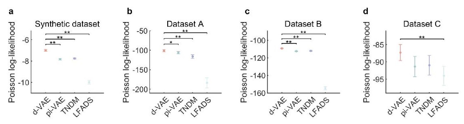
Regarding how R2 is computed:  , where
  and
and  denote ith sample of raw signals, ith sample of distilled relevant signals, and the mean of raw signals. If the distilled signals exactly match the raw signals, the sum of squared error is zero, thus R2=1. If the distilled signals
  always are equal to
  R2=0. If the distilled signals are worse than the mean estimation, R2 is negative, negative R2 is set to zero.
Thank you for your valuable feedback.
Q3: “Third, and relating to this issue, I could not entirely follow the reasoning in the section arguing that behavioural information can be inferred from neurons with weak selectivity, but that it is not linearly decodable. It is right to test if weak supervision signals bleed into the irrelevant subspace, but I could not follow the explanations. Why, for instance, is the ANN decoder on raw data (I assume this is a decoder trained fully supervised) not equal in performance to the revenant distilled signals? Should a well-trained non-linear decoder not simply yield a performance ceiling? Next, if I understand correctly, distilled signals were obtained from the full model. How does a model perform trained only on the weakly tuned neurons? Is it possible that the subspaces obtained with the model are just not optimally aligned for decoding? This could be a result of limited identifiability or model specifics that bias reconstruction to averages (a well-known problem of VAEs). I, therefore, think this analysis should be complemented with tests that do not depend on the model.”
Regarding “Why, for instance, is the ANN decoder on raw data (I assume this is a decoder trained fully supervised) not equal in performance to the relevant distilled signals? Should a well-trained non-linear decoder not simply yield a performance ceiling?”: In fact, the decoding performance of raw signals with ANN is quite close to the ceiling. However, due to the presence of significant irrelevant signals in raw signals, decoding models like deep neural networks are more prone to overfitting when trained on noisy raw signals compared to behaviorally-relevant signals. Consequently, we anticipate that the distilled signals will demonstrate superior decoding generalization. This phenomenon is evident in Fig. 2 and Fig. S1, where the decoding performance of the distilled signals surpasses that of the raw signals, albeit not by a substantial margin.
Regarding “Next, if I understand correctly, distilled signals were obtained from the full model. How does a model perform trained only on the weakly tuned neurons? Is it possible that the subspaces obtained with the model are just not optimally aligned for decoding?”:Distilled signals (involving all neurons) are obtained by d-VAE. Subsequently, we use ANN to evaluate the performance of smaller and larger R2 neurons. Please note that separating and evaluating relevant signals are two distinct stages.
Regarding the reasoning in the section arguing that smaller R2 neurons encode rich information, we would like to provide a detailed explanation:
1) After extracting relevant signals through d-VAE, we specifically selected neurons characterized by smaller R2 values (Here, R2 signifies the proportion of neuronal activity variance explained by the linear encoding model, calculated using raw signals). Subsequently, we employed both KF and ANN to assess the decoding performance of these neurons. Remarkably, our findings revealed that smaller R2 neurons, previously believed to carry limited behavioral information, indeed encode rich information.
2) In a subsequent step, we employed d-VAE to exclusively distill the raw signals of these smaller R2 neurons (distinct from the earlier experiment where d-VAE processed signals from all neurons). We then employed KF and ANN to evaluate the distilled smaller R2 neurons. Interestingly, we observed that we could not attain the same richness of information solely through the use of these smaller R2 neurons.
3) Consequently, we put forth and tested two hypotheses: First, that larger R2 neurons introduce additional signals into the smaller R2 neurons that do not exist in the real smaller R2 neurons. Second, that larger R2 neurons aid in restoring the original appearance of impaired smaller R2 neurons. Our proposed criteria and synthetic experiments substantiate the latter scenario.
Thank you for your valuable feedback.
Q4: “Finally, a more technical issue to note is related to the choice to learn a non-parametric prior instead of using a conventional Gaussian prior. How is this implemented? Is just a single sample taken during a forward pass? I worry this may be insufficient as this would not sample the prior well, and some other strategy such as importance sampling may be required (unless the prior is not relevant as it weakly contributed to the ELBO, in which case this choice seems not very relevant). Generally, it would be useful to see visualisations of the latent variables to see how information about behaviour is represented by the model.”
Regarding "how to implement the prior?": Please refer to Equation 7 in the revised manuscript; we have added detailed descriptions in the revised manuscript.
Regarding "Generally, it would be useful to see visualizations of the latent variables to see how information about behavior is represented by the model.": Note that our focus is not on latent variables but on distilled relevant signals. Nonetheless, at your request, we have added the visualization of latent variables in the revised manuscript. Please see Fig. S13 for details.
Thank you for your valuable feedback.
Recommendations: “A minor point: the word 'distill' in the name of the model may be a little misleading - in machine learning the term refers to the construction of smaller models with the same capabilities.
It should be useful to add a schematic picture of the model to ease comparison with related approaches.”
In the context of our model's functions, it operates as a distillation process, eliminating irrelevant signals and retaining the relevant ones. Although the name of our model may be a little misleading, it faithfully reflects what our model does.
I have added a schematic picture of d-VAE in the revised manuscript. Please see Fig. S1 for details.
Thank you for your valuable feedback.
Reviewer #2
Q1: “Is the apparently increased complexity of encoding vs decoding so unexpected given the entropy, sparseness, and high dimensionality of neural signals (the "encoding") compared to the smoothness and low dimensionality of typical behavioural signals (the "decoding") recorded in neuroscience experiments? This is the title of the paper so it seems to be the main result on which the authors expect readers to focus. ”
We use the term "unexpected" due to the disparity between our findings and the prior understanding concerning neural encoding and decoding. For neural encoding, as we said in the Introduction, in previous studies, weakly-tuned neurons are considered useless, and smaller variance PCs are considered noise, but we found they encode rich behavioral information. For neural decoding, the nonlinear decoding performance of raw signals is significantly superior to linear decoding. However, after eliminating the interference of irrelevant signals, we found the linear decoding performance is comparable to nonlinear decoding. Rooted in these findings, which counter previous thought, we employ the term "unexpected" to characterize our observations.
Thank you for your valuable feedback.
Q2: “I take issue with the premise that signals in the brain are "irrelevant" simply because they do not correlate with a fixed temporal lag with a particular behavioural feature hand-chosen by the experimenter. As an example, the presence of a reward signal in motor cortex [1] after the movement is likely to be of little use from the perspective of predicting kinematics from time-bin to time-bin using a fixed model across trials (the apparent definition of "relevant" for behaviour here), but an entire sub-field of neuroscience is dedicated to understanding the impact of these reward-related signals on future behaviour. Is there method sophisticated enough to see the behavioural "relevance" of this brief, transient, post-movement signal? This may just be an issue of semantics, and perhaps I read too much into the choice of words here. Perhaps the authors truly treat "irrelevant" and "without a fixed temporal correlation" as synonymous phrases and the issue is easily resolved with a clarifying parenthetical the first time the word "irrelevant" is used. But I remain troubled by some claims in the paper which lead me to believe that they read more deeply into the "irrelevancy" of these components.”
In this paper, we employ terms like ‘behaviorally-relevant’ and ‘behaviorally-irrelevant’ only regarding behavioral variables of interest measured within a given task, such as arm kinematics during a motor control task. A similar definition can be found in the PSID[1].
Thank you for your valuable feedback.
[1] Sani, Omid G., et al. "Modeling behaviorally relevant neural dynamics enabled by preferential subspace identification." Nature Neuroscience 24.1 (2021): 140-149.
Q3: “The authors claim the "irrelevant" responses underpin an unprecedented neuronal redundancy and reveal that movement behaviors are distributed in a higher-dimensional neural space than previously thought." Perhaps I just missed the logic, but I fail to see the evidence for this. The neural space is a fixed dimensionality based on the number of neurons. A more sparse and nonlinear distribution across this set of neurons may mean that linear methods such as PCA are not effective ways to approximate the dimensionality. But ultimately the behaviourally relevant signals seem quite low-dimensional in this paper even if they show some nonlinearity may help.”
The evidence for the “useless” responses underpin an unprecedented neuronal redundancy is shown in Fig. 5a, d and Fig. S9a. Specifically, the sum of the decoding performance of smaller R2 neurons and larger R2 neurons is significantly greater than that of all neurons for relevant signals (red bar), demonstrating that movement parameters are encoded very redundantly in neuronal population. In contrast, we can not find this degree of neural redundancy in raw signals (purple bar).
The evidence for the “useless” responses reveal that movement behaviors are distributed in a higher-dimensional neural space than previously thought is shown in the left plot (involving KF decoding) of Fig. 6c, f and Fig. S9f. Specifically, the improvement of KF using secondary signals is significantly higher than using raw signals composed of the same number of dimensions as the secondary signals. These results demonstrate that these dimensions, spanning roughly from ten to thirty, encode much information, suggesting that behavioral information exists in a higher-dimensional subspace than anticipated from raw signals.
Thank you for your valuable feedback.
Q5: “there is an apparent logical fallacy that begins in the abstract and persists in the paper: "Surprisingly, when incorporating often-ignored neural dimensions, behavioral information can be decoded linearly as accurately as nonlinear decoding, suggesting linear readout is performed in motor cortex." Don't get me wrong: the equivalency of linear and nonlinear decoding approaches on this dataset is interesting, and useful for neuroscientists in a practical sense. However, the paper expends much effort trying to make fundamental scientific claims that do not feel very strongly supported. This reviewer fails to see what we can learn about a set of neurons in the brain which are presumed to "read out" from motor cortex. These neurons will not have access to the data analyzed here. That a linear model can be conceived by an experimenter does not imply that the brain must use a linear model. The claim may be true, and it may well be that a linear readout is implemented in the brain. Other work [2,3] has shown that linear readouts of nonlinear neural activity patterns can explain some behavioural features. The claim in this paper, however, is not given enough”
Due to the limitations of current observational methods and our incomplete understanding of brain mechanisms, it is indeed challenging to ascertain the specific data the brain acquires to generate behavior and whether it employs a linear readout. Conventionally, the neural data recorded in the motor cortex do encode movement behaviors and can be used to analyze neural encoding and decoding. Based on these data, we found that the linear decoder KF achieves comparable performance to that of the nonlinear decoder ANN on distilled relevant signals. This finding has undergone validation across three widely used datasets, providing substantial evidence. Furthermore, we conducted experiments on synthetic data to show that this conclusion is not a by-product of our model. In the revised manuscript, we added a more detailed description of this conclusion.
Thank you for your valuable feedback.
Q6: “Relatedly, I would like to note that the exercise of arbitrarily dividing a continuous distribution of a statistic (the "R2") based on an arbitrary threshold is a conceptually flawed exercise. The authors read too much into the fact that neurons which have a low R2 w.r.t. PDs have behavioural information w.r.t. other methods. To this reviewer, it speaks more about the irrelevance, so to speak, of the preferred direction metric than anything fundamental about the brain.”
We chose the R2 threshold in accordance with the guidelines provided in reference [1]. It's worth mentioning that this threshold does not exert any significant influence on the overall conclusions.
Thank you for your valuable feedback.
[1] Inoue, Y., Mao, H., Suway, S.B., Orellana, J. and Schwartz, A.B., 2018. Decoding arm speed during reaching. Nature communications, 9(1), p.5243.
Q7: “I am afraid I may be missing something, as I did not understand the fano factor analysis of Figure 3. In a sense the behaviourally relevant signals must have lower FF given they are in effect tied to the temporally smooth (and consistent on average across trials) behavioural covariates. The point of the original Churchland paper was to show that producing a behaviour squelches the variance; naturally these must appear in the behaviourally relevant components. A control distribution or reference of some type would possibly help here.”
We agree that including reference signals could provide more context. The Churchland paper said stimulus onset can lead to a reduction in neural variability. However, our experiment focuses specifically on the reaching process, and thus, we don't have comparative experiments involving different types of signals.
Thank you for your valuable feedback.
Q8: “The authors compare the method to LFADS. While this is a reasonable benchmark as a prominent method in the field, LFADS does not attempt to solve the same problem as d-VAE. A better and much more fair comparison would be TNDM [4], an extension of LFADS which is designed to identify behaviourally relevant dimensions.”
We have added the comparison experiments with TNDM in the revised manuscript (see Fig. 2 and Fig. S2). The details of model hyperparameters and training settings can be found in the Methods section in the revised manuscripts.
Thank you for your valuable feedback.
Reviewer #3
Q1.1: “TNDM: LFADS is not the best baseline for comparison. The authors should have compared with TNDM (Hurwitz et al. 2021), which is an extension of LFADS that (unlike LFADS) actually attempts to extract behaviorally relevant factors by adding a behavior term to the loss. The code for TNDM is also available on Github. LFADS is not even supervised by behavior and does not aim to address the problem that d-VAE aims to address, so it is not the most appropriate comparison. ”
We have added the comparison experiments with TNDM in the revised manuscript (see Fig. 2 and Fig. S2). The details of model hyperparameters and training settings can be found in the Methods section in the revised manuscripts.
Thank you for your valuable feedback.
Q1.2: “LFADS: LFADS is a sequential autoencoder that processes sections of data (e.g. trials). No explanation is given in Methods for how the data was passed to LFADS. Was the moving averaged smoothed data passed to LFADS or the raw spiking data (at what bin size)? Was a gaussian loss used or a poisson loss? What are the trial lengths used in each dataset, from which part of trials? For dataset C that has back-to-back reaches, was data chopped into segments? How long were these segments? Were the edges of segments overlapped and averaged as in (Keshtkaran et al. 2022) to avoid noisy segment edges or not? These are all critical details that are not explained. The same details would also be needed for a TNDM comparison (comment 1.1) since it has largely the same architecture as LFADS.
It is also critical to briefly discuss these fundamental differences between the inputs of methods in the main text. LFADS uses a segment of data whereas VAE methods just use one sample at a time. What does this imply in the results? I guess as long as VAEs outperform LFADS it is ok, but if LFADS outperforms VAEs in a given metric, could it be because it received more data as input (a whole segment)? Why was the factor dimension set to 50? I presume it was to match the latent dimension of the VAE methods, but is the LFADS factor dimension the correct match for that to make things comparable?
I am also surprised by the results. How do the authors justify LFADS having lower neural similarity (fig 2d) than VAE methods that operate on single time steps? LFADS is not supervised by behavior, so of course I don't expect it to necessarily outperform methods on behavior decoding. But all LFADS aims to do is to reconstruct the neural data so at least in this metric it should be able to outperform VAEs that just operate on single time steps? Is it because LFADS smooths the data too much? This is important to discuss and show examples of. These are all critical nuances that need to be discussed to validate the results and interpret them.”
Regarding “Was the moving averaged smoothed data passed to LFADS or the raw spiking data (at what bin size)? Was a gaussian loss used or a poisson loss?”: The data used by all models was applied to the same preprocessing procedure. That is, using moving averaged smoothed data with three bins, where the bin size is 100ms. For all models except PSID, we used a Poisson loss.
Regrading “What are the trial lengths used in each dataset, from which part of trials? For dataset C that has back-to-back reaches, was data chopped into segments? How long were these segments? Were the edges of segments overlapped and averaged as in (Keshtkaran et al. 2022) to avoid noisy segment edges or not?”:
For datasets A and B, a trial length of eighteen is set. Trials with lengths below the threshold are zero-padded, while trials exceeding the threshold are truncated to the threshold length from their starting point. In dataset A, there are several trials with lengths considerably longer than that of most trials. We found that padding all trials with zeros to reach the maximum length (32) led to poor performance. Consequently, we chose a trial length of eighteen, effectively encompassing the durations of most trials and leading to the removal of approximately 9% of samples. For dataset B (center-out), the trial lengths are relatively consistent with small variation, and the maximum length across all trials is eighteen. For dataset C, we set the trial length as ten because we observed the video of this paradigm and found that the time for completing a single trial was approximately one second. The segments are not overlapped.
Regarding “Why was the factor dimension set to 50? I presume it was to match the latent dimension of the VAE methods, but is the LFADS factor dimension the correct match for that to make things comparable?”: We performed a grid search for latent dimensions in {10,20,50} and found 50 is the best.
Regarding “I am also surprised by the results. How do the authors justify LFADS having lower neural similarity (fig 2d) than VAE methods that operate on single time steps? LFADS is not supervised by behavior, so of course I don't expect it to necessarily outperform methods on behavior decoding. But all LFADS aims to do is to reconstruct the neural data so at least in this metric it should be able to outperform VAEs that just operate on single time steps? Is it because LFADS smooths the data too much?”: As you pointed out, we found that LFADS tends to produce excessively smooth and consistent data, which can lead to a reduction in neural similarity.
Thank you for your valuable feedback.
Q1.3: “PSID: PSID is linear and uses past input samples to predict the next sample in the output. Again, some setup choices are not well justified, and some details are left out in the 1-line explanation given in Methods.
Why was a latent dimension of 6 chosen? Is this the behaviorally relevant latent dimension or the total latent dimension (for the use case here it would make sense to set all latent states to be behaviorally relevant)? Why was a horizon hyperparameter of 3 chosen? First, it is important to mention fundamental parameters such as latent dimension for each method in the main text (not just in methods) to make the results interpretable. Second, these hyperparameters should be chosen with a grid search in each dataset (within the training data, based on performance on the validation part of the training data), just as the authors do for their method (line 779). Given that PSID isn't a deep learning method, doing a thorough grid search in each fold should be quite feasible. It is important that high values for latent dimension and a wider range of other hyperparmeters are included in the search, because based on how well the residuals (x_i) for this method are shown predict behavior in Fig 2, the method seems to not have been used appropriately. I would expect ANN to improve decoding for PSID versus its KF decoding since PSID is fully linear, but I don't expect KF to be able to decode so well using the residuals of PSID if the method is used correctly to extract all behaviorally relevant information from neural data. The low neural reconstruction in Fid 2d could also partly be due to using too small of a latent dimension.
Again, another import nuance is the input to this method and how differs with the input to VAE methods. The learned PSID model is a filter that operates on all past samples of input to predict the output in the "next" time step. To enable a fair comparison with VAE methods, the authors should make sure that the last sample "seen" by PSID is the same as then input sample seen by VAE methods. This is absolutely critical given how large the time steps are, otherwise PSID might underperform simply because it stopped receiving input 300ms earlier than the input received by VAE methods. To fix this, I think the authors can just shift the training and testing neural time series of PSID by 1 sample into the past (relative to the behavior), so that PSID's input would include the input of VAE methods. Otherwise, VAEs outperforming PSID is confounded by PSID's input not including the time step that was provided to VAE.”
Thanks for your suggestions for letting PSID see the current neural observations. We did it per your suggestions and then performed a grid search for the hyperparameters for PSID. Specifically, we performed a grid search for the horizon hyperparameter in {2,3,4,5,6,7}. Since the relevant latent dimension should be lower than the horizon times the dimension of behavior variables (two-dimensional velocity in this paper) and increasing the dimension will reach performance saturation, we directly set the relevant latent dimensions as the maximum. The horizon number of datasets A, B, C, and synthetic datasets is 7, 6, 6 and 5, respectively.
And thus the latent dimension of datasets A, B, and C and the synthetic dataset is 14, 12, 12 and 10, respectively.
Our experiments show that KF can decode information from irrelevant signals obtained by PSID. Although PSID extracts the linear part of raw signals, KF can still use the linear part of the residuals for decoding. The low reconstruction performance of PSID may be because the relationship between latent variables and neural signals is linear, and the relationship between latent variables and behaviors is also linear; this is equivalent to the linear relationship between behaviors and neural signals, and linear models can only explain a small fraction of neural signals.
Thank you for your valuable feedback.
Q1.4: “CEBRA: results for CEBRA are incomplete. Similarity to raw signals is not shown. Decoding of behaviorally irrelevant residuals for CEBRA is not shown. Per Fig. S2, CEBRA does better or similar ANN decoding in datasets A and C, is only slightly worse in Dataset B, so it is important to show the other key metrics otherwise it is unclear whether d-VAE has some tangible advantage over CEBRA in those 2 datasets or if they are similar in every metric. Finally, it would be better if the authors show the results for CEBRA on Fig. 2, just as is done for other methods because otherwise it is hard to compare all methods.”
CEBRA is a non-generative model, this model cannot generate behaviorally-relevant signals. Therefore, we only compared the decoding performance of latent embeddings of CEBRA and signals of d-VAE.
Thank you for your valuable feedback.
Q2: “Given the fact that d-VAE infers the latent (z) based on the population activity (x), claims about properties of the inferred behaviorally relevant signals (x_r) that attribute properties to individual neurons are confounded.
The authors contrast their approach to population level approaches in that it infers behaviorally relevant signals for individual neurons. However, d-VAE is also a population method as it aggregates population information to infer the latent (z), from which behaviorally relevant part of the activity of each neuron (x_r) is inferred. The authors note this population level aggregation of information as a benefit of d-VAE, but only acknowledge it as a confound briefly in the context of one of their analyses (line 340): "The first is that the larger R2 neurons leak their information to the smaller R2 neurons, causing them contain too much behavioral information". They go on to dismiss this confounding possibility by showing that the inferred behaviorally relevant signal of each neuron is often most similar to its own raw signals (line 348-352) compared with all other neurons. They also provide another argument specific to that result section (i.e., residuals are not very behavior predictive), which is not general so I won't discuss it in depth here. These arguments however do not change the basic fact that d-VAE aggregates information from other neurons when extracting the behaviorally relevant activity of any given neuron, something that the authors note as a benefit of d-VAE in many instances. The fact that d-VAE aggregates population level info to give the inferred behaviorally relevant signal for each neuron confounds several key conclusions. For example, because information is aggregated across neurons, when trial to trial variability looks smoother after applying d-VAE (Fig 3i), or reveals better cosine tuning (Fig 3b), or when neurons that were not very predictive of behavior become more predictive of behavior (Fig 5), one cannot really attribute the new smoother single trial activity or the improved decoding to the same single neurons; rather these new signals/performances include information from other neurons. Unless the connections of the encoder network (z=f(x)) is zero for all other neurons, one cannot claim that the inferred rates for the neuron are truly solely associated with that neuron. I believe this a fundamental property of a population level VAE, and simply makes the architecture unsuitable for claims regarding inherent properties of single neurons. This confound is partly why the first claim in the abstract are not supported by data: observing that neurons that don't predict behavior very well would predict it much better after applying d-VAE does not prove that these neurons themselves "encode rich[er] behavioral information in complex nonlinear ways" (i.e., the first conclusion highlighted in the abstract) because information was also aggregated from other neurons. The other reason why this claim is not supported by data is the characterization of the encoding for smaller R2 neurons as "complex nonlinear", which the method is not well equipped to tease apart from linear mappings as I explain in my comment 3.”
We acknowledge that we cannot obtain the exact single neuronal activity that does not contain any information from other neurons. However, we believe our model can extract accurate approximation signals of the ground truth relevant signals. These signals preserve the inherent properties of single neuronal activity to some extent and can be used for analysis at the single-neuron level.
We believe d-VAE is a reasonable approach to extract effective relevant signals that preserve inherent properties of single neuronal activity for four key reasons:
1) d-VAE is a latent variable model that adheres to the neural population doctrine. The neural population doctrine posits that information is encoded within interconnected groups of neurons, with the existence of latent variables (neural modes) responsible for generating observable neuronal activity [1, 2]. If we can perfectly obtain the true generative model from latent variables to neuronal activity, then we can generate the activity of each neuron from hidden variables without containing any information from other neurons. However, without a complete understanding of the brain’s encoding strategies (or generative model), we can only get the approximation signals of the ground truth signals.
2) After the generative model is established, we need to infer the parameters of the generative model and the distribution of latent variables. During the inference process, inference algorithms such as variational inference or EM algorithms will be used. Generally, the obtained latent variables are also approximations of the real latent variables. When inferring the latent variables, it is inevitable to aggregation the information of the neural population, and latent variables are derived through weighted combinations of neuronal populations [3].
This inference process is consistent with that of d-VAE (or VAE-based models).
3) Latent variables are derived from raw neural signals and used to explain raw neural signals. Considering the unknown ground truth of latent variables and behaviorally-relevant signals, it becomes evident that the only reliable reference at the signal level is the raw signals. A crucial criterion for evaluating the reliability of latent variable models (including latent variables and generated relevant signals) is their capability to effectively explain the raw signals [3]. Consequently, we firmly maintain the belief that if the generated signals closely resemble the raw signals to the greatest extent possible, in accordance with an equivalence principle, we can claim that these obtained signals faithfully retain the inherent properties of single neurons. d-VAE explicitly constrains the generated signal to closely resemble the raw signals. These results demonstrate that d-VAE can extract effective relevant signals that preserve inherent properties of single neuronal activity.
Based on the above reasons, we hold that generating single neuronal activities with the VAE framework is a reasonable approach. The remaining question is whether our model can obtain accurate relevant signals in the absence of ground truth. To our knowledge, in cases where the ground truth of relevant signals is unknown, there are typically two approaches to verifying the reliability of extracted signals:
1) Conducting synthetic experiments where the ground truth is known.
2) Validation based on expert knowledge (Three criteria were proposed in this paper). Both our extracted signals and key conclusions have been validated using these two approaches.
Next, we will provide a detailed response to the concerns regarding our first key conclusion that smaller R2 neurons encode rich information.
We acknowledge that larger R2 neurons play a role in aiding the reconstruction of signals in smaller R2 neurons through their neural activity. However, considering that neurons are correlated rather than independent entities, we maintain the belief that larger R2 neurons assist damaged smaller R2 neurons in restoring their original appearance. Taking image denoising as an example, when restoring noisy pixels to their original appearance, relying solely on the noisy pixels themselves is often impractical. Assistance from their correlated, clean neighboring pixels becomes necessary.
The case we need to be cautious of is that the larger R2 neurons introduce additional signals (m) that contain substantial information to smaller R2 neurons, which they do not inherently possess. We believe this case does not hold for two reasons. Firstly, logically, adding extra signals decreases the reconstruction performance, and the information carried by these additional signals is redundant for larger R2 neurons, thus they do not introduce new information that can enhance the decoding performance of the neural population. Therefore, it seems unlikely and unnecessary for neural networks to engage in such counterproductive actions. Secondly, even if this occurs, our second criterion can effectively exclude the selection of these signals. To clarify, if we assume that x, y, and z denote the raw, relevant, and irrelevant signals of smaller R2 neurons, with x=y+z, and the extracted relevant signals become y+m, the irrelevant signals become z-m in this case. Consequently, the irrelevant signals contain a significant amount of information. It's essential to emphasize that this criterion holds significant importance in excluding undesirable signals.
Furthermore, we conducted a synthetic experiment to show that d-VAE can indeed restore the damaged information of smaller R2 neurons with the help of larger R2 neurons, and the restored neuronal activities are more similar to ground truth compared to damaged raw signals. Please see Fig. S11a,b for details.
Thank you for your valuable feedback.
[1] Saxena, S. and Cunningham, J.P., 2019. Towards the neural population doctrine. Current opinion in neurobiology, 55, pp.103-111.
[2] Gallego, J.A., Perich, M.G., Miller, L.E. and Solla, S.A., 2017. Neural manifolds for the control of movement. Neuron, 94(5), pp.978-984.
[3] Cunningham, J.P. and Yu, B.M., 2014. Dimensionality reduction for large-scale neural recordings. Nature neuroscience, 17(11), pp.1500-1509.
Q3: “Given the nonlinear architecture of the VAE, claims about the linearity or nonlinearity of cortical readout are confounded and not supported by the results.
The inference of behaviorally relevant signals from raw signals is a nonlinear operation, that is x_r=g(f(x)) is nonlinear function of x. So even when a linear KF is used to decode behavior from the inferred behaviorally relevant signals, the overall decoding from raw signals to predicted behavior (i.e., KF applied to g(f(x))) is nonlinear. Thus, the result that decoding of behavior from inferred behaviorally relevant signals (x_r) using a linear KF and a nonlinear ANN reaches similar accuracy (Fig 2), does not suggest that a "linear readout is performed in the motor cortex", as the authors claim (line 471). The authors acknowledge this confound (line 472) but fail to address it adequately. They perform a simulation analysis where the decoding gap between KF and ANN remains unchanged even when d-VAE is used to infer behaviorally relevant signals in the simulation. However, this analysis is not enough for "eliminating the doubt" regarding the confound. I'm sure the authors can also design simulations where the opposite happens and just like in the data, d-VAE can improve linear decoding to match ANN decoding. An adequate way to address this concern would be to use a fully linear version of the autoencoder where the f(.) and g(.) mappings are fully linear. They can simply replace these two networks in their model with affine mappings, redo the modeling and see if the model still helps the KF decoding accuracy reach that of the ANN decoding. In such a scenario, because the overall KF decoding from original raw signals to predicted behavior (linear d-VAE + KF) is linear, then they could move toward the claim that the readout is linear. Even though such a conclusion would still be impaired by the nonlinear reference (d-VAE + ANN decoding) because the achieved nonlinear decoding performance could always be limited by network design and fitting issues. Overall, the third conclusion highlighted in the abstract is a very difficult claim to prove and is unfortunately not supported by the results.”
We aim to explore the readout mechanism of behaviorally-relevant signals, rather than raw signals. Theoretically, the process of removing irrelevant signals should not be considered part of the inherent decoding mechanisms of the relevant signals. Assuming that the relevant signals we extracted are accurate, the conclusion of linear readout is established. On the synthetic data where the ground truth is known, our distilled signals show a significant improvement in neural similarity to the ground truth when compared to raw signals (refer to Fig. S2l). This observation demonstrates that our distilled signals are accurate approximations of the ground truth. Furthermore, on the three widely-used real datasets, our distilled signals meet the stringent criteria we have proposed (see Fig. 2), also providing strong evidence for their accuracy.
Regarding the assertion that we could create simulations in which d-VAE can make signals that are inherently nonlinearly decodable into linearly decodable ones: In reality, we cannot achieve this, as the second criterion can rule out the selection of such signals. Specifically,z=x+y=n^2+y, where z, x, y, and n denote raw signals, relevant signals, irrelevant signals and latent variables. If the relevant signals obtained by d-VAE are n, then these signals can be linear decoded accurately. However, the corresponding irrelevant signals are n^2-n+z; thus, irrelevant signals will have much information, and these extracted relevant signals will not be selected. Furthermore, our synthetic experiments offer additional evidence supporting the conclusion that d-VAE does not make inherently nonlinearly decodable signals become linearly decodable ones. As depicted in Fig. S11c, there exists a significant performance gap between KF and ANN when decoding the ground truth signals of smaller R2 neurons. KF exhibits notably low performance, leaving substantial room for compensation by d-VAE. However, following processing by d-VAE, KF's performance of distilled signals fails to surpass its already low ground truth performance and remains significantly inferior to ANN's performance. These results collectively confirm that our approach does not convert signals that are inherently nonlinearly decodable into linearly decodable ones, and the conclusion of linear readout is not a by-product by d-VAE.
Regarding the suggestion of using linear d-VAE + KF, as discussed in the Discussion section, removing the irrelevant signals requires a nonlinear operation, and linear d-VAE can not effectively separate relevant and irrelevant signals.
Thank you for your valuable feedback.
Q4: “The authors interpret several results as indications that "behavioral information is distributed in a higher-dimensional subspace than expected from raw signals", which is the second main conclusion highlighted in the abstract. However, several of these arguments do not convincingly support that conclusion.
4.1) The authors observe that behaviorally relevant signals for neurons with small principal components (referred to as secondary) have worse decoding with KF but better decoding with ANN (Fig. 6b,e), which also outperforms ANN decoding from raw signals. This observation is taken to suggest that these secondary behaviorally relevant signals encode behavior information in highly nonlinear ways and in a higher dimensions neural space than expected (lines 424 and 428). These conclusions however are confounded by the fact that A) d-VAE uses nonlinear encoding, so one cannot conclude from ANN outperforming KF that behavior is encoded nonlinearly in the motor cortex (see comment 3 above), and B) d-VAE aggregates information across the population so one cannot conclude that these secondary neurons themselves had as much behavior information (see comment 2 above).
4.2) The authors observe that the addition of the inferred behaviorally relevant signals for neurons with small principal components (referred to as secondary) improves the decoding of KF more than it improves the decoding of ANN (red curves in Fig 6c,f). This again is interpreted similarly as in 4.1, and is confounded for similar reasons (line 439): "These results demonstrate that irrelevant signals conceal the smaller variance PC signals, making their encoded information difficult to be linearly decoded, suggesting that behavioral information exists in a higher-dimensional subspace than anticipated from raw signals". This is confounded by because of the two reasons explained in 4.1. To conclude nonlinear encoding based on the difference in KF and ANN decoding, the authors would need to make the encoding/decoding in their VAE linear to have a fully linear decoder on one hand (with linear d-VAE + KF) and a nonlinear decoder on the other hand (with linear d-VAE + ANN), as explained in comment 3.
4.3) From S Fig 8, where the authors compare cumulative variance of PCs for raw and inferred behaviorally relevant signals, the authors conclude that (line 554): "behaviorally-irrelevant signals can cause an overestimation of the neural dimensionality of behaviorally-relevant responses (Supplementary Fig. S8)." However, this analysis does not really say anything about overestimation of "behaviorally relevant" neural dimensionality since the comparison is done with the dimensionality of "raw" signals. The next sentence is ok though: "These findings highlight the need to filter out relevant signals when estimating the neural dimensionality.", because they use the phrase "neural dimensionality" not "neural dimensionality of behaviorally-relevant responses".”
Questions 4.1 and 4.2 are a combination of Q2 and Q3. Please refer to our responses to Q2 and Q3.
Regarding question 4.3 about “behaviorally-irrelevant signals can cause an overestimation of the neural dimensionality of behaviorally-relevant responses”: Previous studies usually used raw signals to estimate the neural dimensionality of specific behaviors. We mean that using raw signals, which include many irrelevant signals, will cause an overestimation of the neural dimensionality. We have modified this sentence in the revised manuscripts.
Thank you for your valuable feedback.
Q5: “Imprecise use of language in many places leads to inaccurate statements. I will list some of these statements”
5.1) In the abstract: "One solution is to accurately separate behaviorally-relevant and irrelevant signals, but this approach remains elusive due to the unknown ground truth of behaviorally-relevant signals". This statement is not accurate because it implies no prior work does this. The authors should make their statement more specific and also refer to some goal that existing linear (e.g., PSID) and nonlinear (e.g., TNDM) methods for extracting behaviorally relevant signals fail to achieve.
5.2) In the abstract: "we found neural responses previously considered useless encode rich behavioral information" => what does "useless" mean operationally? Low behavior tuning? More precise use of language would be better.
5.3) "... recent studies (Glaser 58 et al., 2020; Willsey et al., 2022) demonstrate nonlinear readout outperforms linear readout." => do these studies show that nonlinear "readout" outperforms linear "readout", or just that nonlinear models outperform linear models?
5.4) Line 144: "The first criterion is that the decoding performance of the behaviorally-relevant signals (red bar, Fig.1) should surpass that of raw signals (the red dotted line, Fig.1).". Do the authors mean linear decoding here or decoding in general? If the latter, how can something extracted from neural surpass decoding of neural data, when the extraction itself can be thought of as part of decoding? The operational definition for this "decoding performance" should be clarified.
5.5) Line 311: "we found that the dimensionality of primary subspace of raw signals (26, 64, and 45 for datasets A, B, and C) is significantly higher than that of behaviorally-relevant signals (7, 13, and 9), indicating that behaviorally-irrelevant signals lead to an overestimation of the neural dimensionality of behaviorally-relevant signals." => here the dimensionality of the total PC space (i.e., primary subspace of raw signals) is being compared with that of inferred behaviorally-relevant signals, so the former being higher does not indicate that neural dimensionality of behaviorally-relevant signals was overestimated. The former is simply not behavioral so this conclusion is not accurate.
5.6) Section "Distilled behaviorally-relevant signals uncover that smaller R2 neurons encode rich behavioral information in complex nonlinear ways". Based on what kind of R2 are the neurons grouped? Behavior decoding R2 from raw signals? Using what mapping? Using KF? If KF is used, the result that small R2 neurons benefit a lot from d-VAE could be somewhat expected, given the nonlinearity of d-VAE: because only ANN would have the capacity to unwrap the nonlinear encoding of d-VAE as needed. If decoding performance that is used to group neurons is based on data, regression to the mean could also partially explain the result: the neurons with worst raw decoding are most likely to benefit from a change in decoder, than neurons that already had good decoding. In any case, the R2 used to partition and sort neurons should be more clearly stated and reminded throughout the text and I Fig 3.
5.7) Line 346 "...it is impossible for our model to add the activity of larger R2 neurons to that of smaller R2 neurons" => Is it really impossible? The optimization can definitely add small-scale copies of behaviorally relevant information to all neurons with minimal increase in the overall optimization loss, so this statement seems inaccurate.
5.8) Line 490: "we found that linear decoders can achieve comparable performance to that of nonlinear decoders, providing compelling evidence for the presence of linear readout in the motor cortex." => inaccurate because no d-VAE decoding is really linear, as explained in comment 3 above.
5.9) Line 578: ". However, our results challenge this idea by showing that signals composed of smaller variance PCs nonlinearly encode a significant amount of behavioral information." => inaccurate as results are confounded by nonlinearity of d-VAE as explained in comment 3 above.
5.10) Line 592: "By filtering out behaviorally-irrelevant signals, our study found that accurate decoding performance can be achieved through linear readout, suggesting that the motor cortex may perform linear readout to generate movement behaviors." => inaccurate because it us confounded by the nonlinearity of d-VAE as explained in comment 3 above.”
Regarding “5.1) In the abstract: "One solution is to accurately separate behaviorally-relevant and irrelevant signals, but this approach remains elusive due to the unknown ground truth of behaviorally-relevant signals". This statement is not accurate because it implies no prior work does this. The authors should make their statement more specific and also refer to some goal that existing linear (e.g., PSID) and nonlinear (e.g., TNDM) methods for extracting behaviorally relevant signals fail to achieve”:
We believe our statement is accurate. Our primary objective is to extract accurate behaviorally-relevant signals that closely approximate the ground truth relevant signals. To achieve this, we strike a balance between the reconstruction and decoding performance of the generated signals, aiming to effectively capture the relevant signals. This crucial aspect of our approach sets it apart from other methods. In contrast, other methods tend to emphasize the extraction of valuable latent neural dynamics. We have provided elaboration on the distinctions between d-VAE and other approaches in the Introduction and Discussion sections.
Thank you for your valuable feedback.
Regarding “5.2) In the abstract: "we found neural responses previously considered useless encode rich behavioral information" => what does "useless" mean operationally? Low behavior tuning? More precise use of language would be better.”:
In the analysis of neural signals, smaller variance PC signals are typically seen as noise and are often discarded. Similarly, smaller R2 neurons are commonly thought to be dominated by noise and are not further analyzed. Given these considerations, we believe that the term "considered useless" is appropriate in this context. Thank you for your valuable feedback.
Regarding “5.3) "... recent studies (Glaser 58 et al., 2020; Willsey et al., 2022) demonstrate nonlinear readout outperforms linear readout." => do these studies show that nonlinear "readout" outperforms linear "readout", or just that nonlinear models outperform linear models?”:
In this paper, we consider the two statements to be equivalent. Thank you for your valuable feedback.
Regarding “5.4) Line 144: "The first criterion is that the decoding performance of the behaviorally-relevant signals (red bar, Fig.1) should surpass that of raw signals (the red dotted line, Fig.1).". Do the authors mean linear decoding here or decoding in general? If the latter, how can something extracted from neural surpass decoding of neural data, when the extraction itself can be thought of as part of decoding? The operational definition for this "decoding performance" should be clarified.”:
We mean the latter, as we said in the section “Framework for defining, extracting, and separating behaviorally-relevant signals”, since raw signals contain too many behaviorally-irrelevant signals, deep neural networks are more prone to overfit raw signals than relevant signals. Therefore the decoding performance of relevant signals should surpass that of raw signals. Thank you for your valuable feedback.
Regarding “5.5) Line 311: "we found that the dimensionality of primary subspace of raw signals (26, 64, and 45 for datasets A, B, and C) is significantly higher than that of behaviorally-relevant signals (7, 13, and 9), indicating that behaviorally-irrelevant signals lead to an overestimation of the neural dimensionality of behaviorally-relevant signals." => here the dimensionality of the total PC space (i.e., primary subspace of raw signals) is being compared with that of inferred behaviorally-relevant signals, so the former being higher does not indicate that neural dimensionality of behaviorally-relevant signals was overestimated. The former is simply not behavioral so this conclusion is not accurate.”: In practice, researchers usually used raw signals to estimate the neural dimensionality. We mean that using raw signals to do this would overestimate the neural dimensionality. Thank you for your valuable feedback.
Regarding “5.6) Section "Distilled behaviorally-relevant signals uncover that smaller R2 neurons encode rich behavioral information in complex nonlinear ways". Based on what kind of R2 are the neurons grouped? Behavior decoding R2 from raw signals? Using what mapping? Using KF? If KF is used, the result that small R2 neurons benefit a lot from d-VAE could be somewhat expected, given the nonlinearity of d-VAE: because only ANN would have the capacity to unwrap the nonlinear encoding of d-VAE as needed. If decoding performance that is used to group neurons is based on data, regression to the mean could also partially explain the result: the neurons with worst raw decoding are most likely to benefit from a change in decoder, than neurons that already had good decoding. In any case, the R2 used to partition and sort neurons should be more clearly stated and reminded throughout the text and I Fig 3.”:
When employing R2 to characterize neurons, it indicates the extent to which neuronal activity is explained by the linear encoding model [1-3]. Smaller R2 neurons have a lower capacity for linearly tuning (encoding) behaviors, while larger R2 neurons have a higher capacity for linearly tuning (encoding) behaviors. Specifically, the approach involves first establishing an encoding relationship from velocity to neural signal using a linear model, i.e., y=f(x), where f represents a linear regression model, x denotes velocity, and y denotes the neural signal. Subsequently, R2 is utilized to quantify the effectiveness of the linear encoding model in explaining neural activity. We have provided a comprehensive explanation in the revised manuscript. Thank you for your valuable feedback.
[1] Collinger, J.L., Wodlinger, B., Downey, J.E., Wang, W., Tyler-Kabara, E.C., Weber, D.J., McMorland, A.J., Velliste, M., Boninger, M.L. and Schwartz, A.B., 2013. High-performance neuroprosthetic control by an individual with tetraplegia. The Lancet, 381(9866), pp.557-564.
[2] Wodlinger, B., et al. "Ten-dimensional anthropomorphic arm control in a human brain− machine interface: difficulties, solutions, and limitations." Journal of neural engineering 12.1 (2014): 016011.
[3] Inoue, Y., Mao, H., Suway, S.B., Orellana, J. and Schwartz, A.B., 2018. Decoding arm speed during reaching. Nature communications, 9(1), p.5243.
Regarding Questions 5.7, 5.8, 5.9, and 5.10:
We believe our conclusions are solid. The reasons can be found in our replies in Q2 and Q3. Thank you for your valuable feedback.
Q6: “Imprecise use of language also sometimes is not inaccurate but just makes the text hard to follow.
6.1) Line 41: "about neural encoding and decoding mechanisms" => what is the definition of encoding/decoding and how do these differ? The definitions given much later in line 77-79 is also not clear.
6.2) Line 323: remind the reader about what R2 is being discussed, e.g., R2 of decoding behavior using KF. It is critical to know if linear or nonlinear decoding is being discussed.
6.3) Line 488: "we found that neural responses previously considered trivial encode rich behavioral information in complex nonlinear ways" => "trivial" in what sense? These phrases would benefit from more precision, for example: "neurons that may seem to have little or no behavior information encoded". The same imprecise word ("trivial") is also used in many other places, for example in the caption of Fig S9.
6.4) Line 611: "The same should be true for the brain." => Too strong of a statement for an unsupported claim suggesting the brain does something along the lines of nonlin VAE + linear readout.
6.5) In Fig 1, legend: what is the operational definition of "generating performance"? Generating what? Neural reconstruction?”
Regarding “6.1) Line 41: "about neural encoding and decoding mechanisms" => what is the definition of encoding/decoding and how do these differ? The definitions given much later in line 77-79 is also not clear.”:
We would like to provide a detailed explanation of neural encoding and decoding. Neural encoding means how neuronal activity encodes the behaviors, that is, y=f(x), where y denotes neural activity and, x denotes behaviors, f is the encoding model. Neural decoding means how the brain decodes behaviors from neural activity, that is, x=g(y), where g is the decoding model. For further elaboration, please refer to [1]. We have included references that discuss the concepts of encoding and decoding in the revised manuscript. Thank you for your valuable feedback.
[1] Kriegeskorte, Nikolaus, and Pamela K. Douglas. "Interpreting encoding and decoding models." Current opinion in neurobiology 55 (2019): 167-179.
Regarding “6.2) Line 323: remind the reader about what R2 is being discussed, e.g., R2 of decoding behavior using KF. It is critical to know if linear or nonlinear decoding is being discussed.”:
This question is the same as Q5.6. Please refer to the response to Q5.6. Thank you for your valuable feedback.
Regarding “6.3) Line 488: "we found that neural responses previously considered trivial encode rich behavioral information in complex nonlinear ways" => "trivial" in what sense? These phrases would benefit from more precision, for example: "neurons that may seem to have little or no behavior information encoded". The same imprecise word ("trivial") is also used in many other places, for example in the caption of Fig S9.”:
We have revised this statement in the revised manuscript. Thanks for your recommendation.
Regarding “6.4) Line 611: "The same should be true for the brain." => Too strong of a statement for an unsupported claim suggesting the brain does something along the lines of nonlin VAE + linear readout.”
We mean that removing the interference of irrelevant signals and decoding the relevant signals should logically be two stages. We have revised this statement in the revised manuscript. Thank you for your valuable feedback.
Regarding “6.5) In Fig 1, legend: what is the operational definition of "generating performance"? Generating what? Neural reconstruction?””:
We have replaced “generating performance” with “reconstruction performance” in the revised manuscript. Thanks for your recommendation.
Q7: “In the analysis presented starting in line 449, the authors compare improvement gained for decoding various speed ranges by adding secondary (small PC) neurons to the KF decoder (Fig S11). Why is this done using the KF decoder, when earlier results suggest an ANN decoder is needed for accurate decoding from these small PC neurons? It makes sense to use the more accurate nonlinear ANN decoder to support the fundamental claim made here, that smaller variance PCs are involved in regulating precise control”
Because when the secondary signal is superimposed on the primary signal, the enhancement in KF performance is substantial. We wanted to explore in which aspect of the behavior the KF performance improvement is mainly reflected. In comparison, the improvement of ANN by the secondary signal is very small, rendering the exploration of the aforementioned questions inconsequential. Thank you for your valuable feedback.
Q8: “A key limitation of the VAE architecture is that it doesn't aggregate information over multiple time samples. This may be why the authors decided to use a very large bin size of 100ms and beyond that smooth the data with a moving average. This limitation should be clearly stated somewhere in contrast with methods that can aggregate information over time (e.g., TNDM, LFADS, PSID) ”
We have added this limitation in the Discussion in the revised manuscript. Thanks for your recommendation.
Q9: “Fig 5c and parts of the text explore the decoding when some neurons are dropped. These results should come with a reminder that dropping neurons from behaviorally relevant signals is not technically possible since the extraction of behaviorally relevant signals with d-VAE is a population level aggregation that requires the raw signal from all neurons as an input. This is also important to remind in some places in the text for example:
Line 498: "...when one of the neurons is destroyed."
Line 572: "In contrast, our results show that decoders maintain high performance on distilled signals even when many neurons drop out."”
We want to explore the robustness of real relevant signals in the face of neuron drop-out. The signals our model extracted are an approximation of the ground truth relevant signals and thus serve as a substitute for ground truth to study this problem. Thank you for your valuable feedback.
Q10: “Besides the confounded conclusions regarding the readout being linear (see comment 3 and items related to it in comment 5), the authors also don't adequately discuss prior works that suggest nonlinearity helps decoding of behavior from the motor cortex. Around line 594, a few works are discussed as support for the idea of a linear readout. This should be accompanied by a discussion of works that support a nonlinear encoding of behavior in the motor cortex, for example (Naufel et al. 2019; Glaser et al. 2020), some of which the authors cite elsewhere but don't discuss here.”
We have added this discussion in the revised manuscript. Thanks for your recommendation.
Q11: “Selection of hyperparameters is not clearly explained. Starting line 791, the authors give some explanation for one hyperparameter, but not others. How are the other hyperparameters determined? What is the search space for the grid search of each hyperparameter? Importantly, if hyperparameters are determined only based on the training data of each fold, why is only one value given for the hyperparameter selected in each dataset (line 814)? Did all 5 folds for each dataset happen to select exactly the same hyperparameter based on their 5 different training/validation data splits? That seems unlikely.”
We perform a grid search in {0.001, 0.01,0.1,1} for hyperparameter beta. And we found that 0.001 is the best for all datasets. As for the model parameters, such as hidden neuron numbers, this model capacity has reached saturation decoding performance and does not influence the results.
Regarding “Importantly, if hyperparameters are determined only based on the training data of each fold, why is only one value given for the hyperparameter selected in each dataset (line 814)? Did all 5 folds for each dataset happen to select exactly the same hyperparameter based on their 5 different training/validation data splits”: We selected the hyperparameter based on the average performance of 5 folds data on validation sets. The selected value denotes the one that yields the highest average performance across the 5 folds data.
Thank you for your valuable feedback.
Q12: “d-VAE itself should also be explained more clearly in the main text. Currently, only the high-level idea of the objective is explained. The explanation should be more precise and include the idea of encoding to latent state, explain the relation to pip-VAE, explain inputs and outputs, linearity/nonlinearity of various mappings, etc. Also see comment 1 above, where I suggest adding more details about other methods in the main text.”
Our primary objective is to delve into the encoding and decoding mechanisms using the separated relevant signals. Therefore, providing an excessive amount of model details could potentially distract from the main focus of the paper. In response to your suggestion, we have included a visual representation of d-VAE's structure, input, and output (see Fig. S1) in the revised manuscript, which offers a comprehensive and intuitive overview. Additionally, we have expanded on the details of d-VAE and other methods in the Methods section.
Thank you for your valuable feedback.
Q13: “In Fig 1f and g, shouldn't the performance plots be swapped? The current plots seem counterintuitive. If there is bias toward decoding (panel g), why is the irrelevant residual so good at decoding?”
The placement of the performance plots in Fig. 1f and 1g is accurate. When the model exhibits a bias toward decoding, it prioritizes extracting the most relevant features (latent variables) for decoding purposes. As a consequence, the model predominantly generates signals that are closely associated with these extracted features. This selective signal extraction and generation process may result in the exclusion of other potentially useful information, which will be left in the residuals. To illustrate this concept, consider the example of face recognition: if a model can accurately identify an individual using only the person's eyes (assuming these are the most useful features), other valuable information, such as details of the nose or mouth, will be left in the residuals, which could also be used to identify the individual.
Thank you for your valuable feedback.
Author Response:
The following is the authors’ response to the previous reviews.
We carefully read through the second-round reviews and the additional reviews. To us, the review process is somewhat unusual and very much dominated by referee 2, who aggressively insists that we mixed up the trigeminal nucleus and inferior olive and that as a consequence our results are meaningless. We think the stance of referee 2 and the focus on one single issue (the alleged mix-up of trigeminal nucleus and inferior olive) is somewhat unfortunate, leaves out much of our findings and we debated at length on how to deal with further revisions. In the end, we decided to again give priority to addressing the criticism of referees 2, because it is hard to go on with a heavily attacked paper without resolving the matter at stake. The following is a summary of, what we did:
Additional experimental work:
(1) We checked if the peripherin-antibody indeed reliably identifies climbing fibers.
To this end, we sectioned the elephant cerebellum and stained sections with the peripherin-antibody. We find: (i) the cerebellar white matter is strongly reactive for peripherin-antibodies, (ii) cerebellar peripherin-antibody staining of has an axonal appearance. (iii) Cerebellar Purkinje cell somata appear to be ensheated by peripherin-antibody staining. (iv) We observed that the peripherin-antibody reactivity gradually decreases from Purkinje cell somata to the pia in the cerebellar molecular layer. This work is shown in our revised Figure 2. All these four features align with the distribution of climbing fibers (which arrive through the white matter, are axons, ensheat Purkinje cell somata, and innervate Purkinje cell proximally not reaching the pia). In line with previous work, which showed similar cerebellar staining patterns in several species (Errante et al. 1998), we conclude that elephant climbing fibers are strongly reactive for peripherin-antibodies.
(2) We delineated the elephant olivo-cerebellar tract.
The strong peripherin-antibody reactivity of elephant climbing fibers enabled us to delineate the elephant olivo-cerebellar tract. We find the elephant olivo-cerebellar tract is a strongly peripherin-antibody reactive, well-delineated fiber tract several millimeters wide and about a centimeter in height. The unstained olivo-cerebellar tract has a greyish appearance. In the anterior regions of the olivo-cerebellar tract, we find that peripherin-antibody reactive fibers run in the dorsolateral brainstem and approach the cerebellar peduncle, where the tract gradually diminishes in size, presumably because climbing fibers discharge into the peduncle. Indeed, peripherin-antibody reactive fibers can be seen entering the cerebellar peduncle. Towards the posterior end of the peduncle, the olivo-cerebellar disappears (in the dorsal brainstem directly below the peduncle. We note that the olivo-cerebellar tract was referred to as the spinal trigeminal tract by Maseko et al. 2013. We think the tract in question cannot be the spinal trigeminal tract for two reasons: (i) This tract is the sole brainstem source of peripherin-positive climbing fibers entering the peduncle/ the cerebellum; this is the defining characteristic of the olivo-cerebellar tract. (ii) The tract in question is much smaller than the trigeminal nerve, disappears posterior to where the trigeminal nerve enters the brainstem (see below), and has no continuity with the trigeminal nerve; the continuity with the trigeminal nerve is the defining characteristic of the spinal trigeminal tract, however.
The anterior regions of the elephant olivo-cerebellar tract are similar to the anterior regions of olivo-cerebellar tract of other mammals in its dorsolateral position and the relation to the cerebellar peduncle. In its more posterior parts, the elephant olivo-cerebellar tract continues for a long distance (~1.5 cm) in roughly the same dorsolateral position and enters the serrated nucleus that we previously identified as the elephant inferior olive. The more posterior parts of the elephant olivo-cerebellar tract therefore differ from the more posterior parts of the olivo-cerebellar tract of other mammals, which follows a ventromedial trajectory towards a ventromedially situated inferior olive. The implication of our delineation of the elephant olivo-cerebellar tract is that we correctly identified the elephant inferior olive.
(3) An in-depth analysis of peripherin-antibody reactivity also indicates that the trigeminal nucleus receives no climbing fiber input.
We also studied the peripherin-antibody reactivity in and around the trigeminal nucleus. We had also noted in the previous submission that the trigeminal nucleus is weakly positive for peripherin, but that the staining pattern is uniform and not the type of axon bundle pattern that is seen in the inferior olive of other mammals. To us, this observation already argued against the presence of climbing fibers in the trigeminal nucleus. We also noted that the myelin stripes of the trigeminal nucleus were peripherin-antibody-negative. In the context of our olivo-cerebellar tract tracing we now also scrutinized the surroundings of the trigeminal nucleus for peripherin-antibody reactivity. We find that the ventral brainstem surrounding the trigeminal nucleus is devoid of peripherin-antibody reactivity. Accordingly, no climbing fibers, (which we have shown to be strongly peripherin-antibody-positive, see our point 1) arrive at the trigeminal nucleus. The absence of climbing fiber input indicates that previous work that identified the (trigeminal) nucleus as the inferior olive (Maseko et al 2013) is unlikely to be correct.
(4) We characterized the entry of the trigeminal nerve into the elephant brain.
To better understand how trigeminal information enters the elephant’s brain, we characterized the entry of the trigeminal nerve. This analysis indicated to us that the trigeminal nerve is not continuous with the olivo-cerebellar tract (the spinal trigeminal tract of Maseko et al. 2013) as previously claimed by Maseko et al. 2013. We show some of this evidence in Referee-Figure 1 below. The reason we think the trigeminal nerve is discontinuous with the olivo-cerebellar tract is the size discrepancy between the two structures. We first show this for the tracing data of Maseko et al. 2013. In the Maseko et al. 2013 data the trigeminal nerve (Referee-Figure 1A, their plate Y) has 3-4 times the diameter of the olivocerebellar tract (the alleged spinal trigeminal tract, Referee-Figure 1B, their plate Z). Note that most if not all trigeminal fibers are thought to continue from the nerve into the trigeminal tract (see our rat data below). We plotted the diameter of the trigeminal nerve and diameter of the olivo-cerebellar (the spinal trigeminal tract according to Maseko et al. 2013) from the Maseko et al. 2013 data (Referee-Figure 1C) and we found that the olivocerebellar tract has a fairly consistent diameter (46 ± 9 mm2, mean ± SD). Statistical considerations and anatomical evidence suggest that the tracing of the trigeminal nerve into the olivo-cerebellar (the spinal trigeminal tract according to Maseko et al. 2013) is almost certainly wrong. The most anterior point of the alleged spinal trigeminal tract has a diameter of 51 mm2 which is more than 15 standard deviations different from the most posterior diameter (194 mm2) of the trigeminal tract. For this assignment to be correct three-quarters of trigeminal nerve fibers would have to spontaneously disappear, something that does not happen in the brain. We also made similar observations in the African elephant Bibi, where the trigeminal nerve (Referee-Figure 1D) is much larger in diameter than the olivocerebellar tract (Referee-Figure 1E). We could also show that the olivocerebellar tract disappears into the peduncle posterior to where the trigeminal nerve enters (Referee-Figure 1F). Our data are very similar to Maseko et al. indicating that their outlining of structures was done correctly. What appears to have been oversimplified, is the assignment of structures as continuous. We also quantified the diameter of the trigeminal nerve and the spinal trigeminal tract in rats (from the Paxinos & Watson atlas; Referee-Figure 1D); as expected we found the trigeminal nerve and spinal trigeminal tract diameters are essentially continuous.
In our hands, the trigeminal nerve does not continue into a well-defined tract that could be traced after its entry. In this regard, it differs both from the olivo-cerebellar tract of the elephant or the spinal trigeminal tract of the rodent, both of which are well delineated. We think the absence of a well-delineated spinal trigeminal tract in elephants might have contributed to the putative tracing error highlighted in our Referee-Figure 1A-C.
We conclude that a size mismatch indicates trigeminal fibers do not run in the olivo-cerebellar tract (the spinal trigeminal tract according to Maseko et al. 2013).
Author response image 1.
The trigeminal nerve is discontinuous with the olivo-cerebellar tract (the spinal trigeminal tract according to Maseko et al. 2013). A, Trigeminal nerve (orange) in the brain of African elephant LAX as delineated by Maseko et al. 2013 (coronal section; their plate Y). B, Most anterior appearance of the spinal trigeminal tract of Maseko et al. 2013 (blue; coronal section; their plate Z). Note the much smaller diameter of the spinal trigeminal tract compared to the trigeminal nerve shown in C, which argues against the continuity of the two structures. Indeed, our peripherin-antibody staining showed that the spinal trigeminal tract of Maseko corresponds to the olivo-cerebellar tract and is discontinuous with the trigeminal nerve. C, Plot of the trigeminal nerve and olivo-cerebellar tracts (the spinal trigeminal tract according to Maseko et al. 2013) diameter along the anterior-posterior axis. The trigeminal nerve is much larger in diameter than the olivocerebellar tract (the spinal trigeminal tract according to Maseko et al. 2013). C, D measurements, for which sections are shown in panels C and D respectively. The olivocerebellar tract (the spinal trigeminal tract according to Maseko et al. 2013) has a consistent diameter; data replotted from Maseko et al. 2013. At mm 25 the inferior olive appears. D, Trigeminal nerve entry in the brain of African elephant Bibi; our data, coronal section, the trigeminal nerve is outlined in orange, note the large diameter. E, Most anterior appearance of the olivo-cerebellar tract in the brain of African elephant Bibi; our data, coronal section, approximately 3 mm posterior to the section shown in A, the olivocerebellar tract is outlined in blue. Note the smaller diameter of the olivo-cerebellar tract compared to the trigeminal nerve, which argues against the continuity of the two structures. F, Plot of the trigeminal nerve and olivo-cerebellar tract diameter along the anterior-posterior axis. The nerve and olivo-cerebellar tract are discontinuous and the trigeminal nerve is much larger in diameter than the olivocerebellar tract (the spinal trigeminal tract according to Maseko et al. 2013); our data. D, E measurements, for which sections are shown in panels D and E respectively. At mm 27 the inferior olive appears. G, In the rat the trigeminal nerve is continuous in size with the spinal trigeminal tract. Data replotted from Paxinos and Watson.
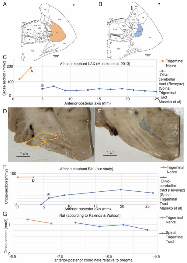
Reviewer 2 (Public Review):
As indicated in my previous review of this manuscript (see above), it is my opinion that the authors have misidentified, and indeed switched, the inferior olivary nuclear complex (IO) and the trigeminal nuclear complex (Vsens). It is this specific point only that I will address in this second review, as this is the crucial aspect of this paper - if the identification of these nuclear complexes in the elephant brainstem by the authors is incorrect, the remainder of the paper does not have any scientific validity.
Comment: We agree with the referee that it is most important to sort out, the inferior olivary nuclear complex (IO) and the trigeminal nuclear complex, respectively.Change: We did additional experimental work to resolve this matter as detailed at the beginning of our response. Specifically, we ascertained that elephant climbing fibers are strongly peripherin-positive. Based on elephant climbing fiber peripherin-reactivity we delineated the elephant olivo-cerebellar tract. We find that the olivo-cerebellar connects to the structure we refer to as inferior olive to the cerebellum (the referee refers to this structure as the trigeminal nuclear complex). We also found that the trigeminal nucleus (the structure the referee refers to as inferior olive) appears to receive no climbing fibers. We provide indications that the tracing of the trigeminal nerve into the olivo-cerebellar tract by Maseko et al. 2023 was erroneous (Author response image 1). These novel findings support our ideas but are very difficult to reconcile with the referee’s partitioning scheme.
The authors, in their response to my initial review, claim that I "bend" the comparative evidence against them. They further claim that as all other mammalian species exhibit a "serrated" appearance of the inferior olive, and as the elephant does not exhibit this appearance, that what was previously identified as the inferior olive is actually the trigeminal nucleus and vice versa.
For convenience, I will refer to IOM and VsensM as the identification of these structures according to Maseko et al (2013) and other authors and will use IOR and VsensR to refer to the identification forwarded in the study under review. <br /> The IOM/VsensR certainly does not have a serrated appearance in elephants. Indeed, from the plates supplied by the authors in response (Referee Fig. 2), the cytochrome oxidase image supplied and the image from Maseko et al (2013) shows a very similar appearance. There is no doubt that the authors are identifying structures that closely correspond to those provided by Maseko et al (2013). It is solely a contrast in what these nuclear complexes are called and the functional sequelae of the identification of these complexes (are they related to the trunk sensation or movement controlled by the cerebellum?) that is under debate.
Elephants are part of the Afrotheria, thus the most relevant comparative data to resolve this issue will be the identification of these nuclei in other Afrotherian species. Below I provide images of these nuclear complexes, labelled in the standard nomenclature, across several Afrotherian species.
(A) Lesser hedgehog tenrec (Echinops telfairi)
Tenrecs brains are the most intensively studied of the Afrotherian brains, these extensive neuroanatomical studies undertaken primarily by Heinz Künzle. Below I append images (coronal sections stained with cresol violet) of the IO and Vsens (labelled in the standard mammalian manner) in the lesser hedgehog tenrec. It should be clear that the inferior olive is located in the ventral midline of the rostral medulla oblongata (just like the rat) and that this nucleus is not distinctly serrated. The Vsens is located in the lateral aspect of the medulla skirted laterally by the spinal trigeminal tract (Sp5). These images and the labels indicating structures correlate precisely with that provide by Künzle (1997, 10.1016, see his Figure 1K,L. Thus, in the first case of a related species, there is no serrated appearance of the inferior olive, the location of the inferior olive is confirmed through connectivity with the superior colliculus (a standard connection in mammals) by Künzle (1997), and the location of Vsens is what is considered to be typical for mammals. This is in agreement with the authors, as they propose that ONLY the elephants show the variations they report.
(B) Giant otter shrew (Potomogale velox)
The otter shrews are close relatives of the Tenrecs. Below I append images of cresyl violet (left column) and myelin (right column) stained coronal sections through the brainstem with the IO, Vsens and Sp5 labelled as per standard mammalian anatomy. Here we see hints of the serration of the IO as defined by the authors, but we also see many myelin stripes across the IO. Vsens is located laterally and skirted by the Sp5. This is in agreement with the authors, as they propose that ONLY the elephants show the variations they report.
(C) Four-toed sengi (Petrodromus tetradactylus)
The sengis are close relatives of the Tenrecs and otter shrews, these three groups being part of the Afroinsectiphilia, a distinct branch of the Afrotheria. Below I append images of cresyl violet (left column) and myelin (right column) stained coronal sections through the brainstem with the IO, Vsens and Sp5 labelled as per standard mammalian anatomy. Here we see vague hints of the serration of the IO (as defined by the authors), and we also see many myelin stripes across the IO. Vsens is located laterally and skirted by the Sp5. This is in agreement with the authors, as they propose that ONLY the elephants show the variations they report.
(D) Rock hyrax (Procavia capensis)
The hyraxes, along with the sirens and elephants form the Paenungulata branch of the Afrotheria. Below I append images of cresyl violet (left column) and myelin (right column) stained coronal sections through the brainstem with the IO, Vsens and Sp5 labelled as per the standard mammalian anatomy. Here we see hints of the serration of the IO (as defined by the authors), but we also see evidence of a more "bulbous" appearance of subnuclei of the IO (particularly the principal nucleus), and we also see many myelin stripes across the IO. Vsens is located laterally and skirted by the Sp5. This is in agreement with the authors, as they propose that ONLY the elephants show the variations they report.
(E) West Indian manatee (Trichechus manatus)
The sirens are the closest extant relatives of the elephants in the Afrotheria. Below I append images of cresyl violet (top) and myelin (bottom) stained coronal sections (taken from the University of Wisconsin-Madison Brain Collection, https://brainmuseum.org, and while quite low in magnification they do reveal the structures under debate) through the brainstem with the IO, Vsens and Sp5 labelled as per standard mammalian anatomy. Here we see the serration of the IO (as defined by the authors). Vsens is located laterally and skirted by the Sp5. This is in agreement with the authors, as they propose that ONLY the elephants show the variations they report.
These comparisons and the structural identification, with which the authors agree as they only distinguish the elephants from the other Afrotheria, demonstrate that the appearance of the IO can be quite variable across mammalian species, including those with a close phylogenetic affinity to the elephants. Not all mammal species possess a "serrated" appearance of the IO. Thus, it is more than just theoretically possible that the IO of the elephant appears as described prior to this study.
So what about elephants? Below I append a series of images from coronal sections through the African elephant brainstem stained for Nissl, myelin, and immunostained for calretinin. These sections are labelled according to standard mammalian nomenclature. In these complete sections of the elephant brainstem, we do not see a serrated appearance of the IOM (as described previously and in the current study by the authors). Rather the principal nucleus of the IOM appears to be bulbous in nature. In the current study, no image of myelin staining in the IOM/VsensR is provided by the authors. However, in the images I provide, we do see the reported myelin stripes in all stains - agreement between the authors and reviewer on this point. The higher magnification image to the bottom left of the plate shows one of the IOM/VsensR myelin stripes immunostained for calretinin, and within the myelin stripes axons immunopositive for calretinin are seen (labelled with an arrow). The climbing fibres of the elephant cerebellar cortex are similarly calretinin immunopositive (10.1159/000345565). In contrast, although not shown at high magnification, the fibres forming the Sp5 in the elephant (in the Maseko description, unnamed in the description of the authors) show no immunoreactivity to calretinin.
Comment: We appreciate the referee’s additional comments. We concede the possibility that some relatives of elephants have a less serrated inferior olive than most other mammals. We maintain, however, that the elephant inferior olive (our Figure 1J) has the serrated appearance seen in the vast majority of mammals.
Change: None.
Peripherin Immunostaining
In their revised manuscript the authors present immunostaining of peripherin in the elephant brainstem. This is an important addition (although it does replace the only staining of myelin provided by the authors which is unusual as the word myelin is in the title of the paper) as peripherin is known to specifically label peripheral nerves. In addition, as pointed out by the authors, peripherin also immunostains climbing fibres (Errante et al., 1998). The understanding of this staining is important in determining the identification of the IO and Vsens in the elephant, although it is not ideal for this task as there is some ambiguity. Errante and colleagues (1998; Fig. 1) show that climbing fibres are peripherin-immunopositive in the rat. But what the authors do not evaluate is the extensive peripherin staining in the rat Sp5 in the same paper (Errante et al, 1998, Fig. 2). The image provided by the authors of their peripherin immunostaining (their new Figure 2) shows what I would call the Sp5 of the elephant to be strongly peripherin immunoreactive, just like the rat shown in Errant et al (1998), and more over in the precise position of the rat Sp5! This makes sense as this is where the axons subserving the "extraordinary" tactile sensitivity of the elephant trunk would be found (in the standard model of mammalian brainstem anatomy). Interestingly, the peripherin immunostaining in the elephant is clearly lamellated...this coincides precisely with the description of the trigeminal sensory nuclei in the elephant by Maskeo et al (2013) as pointed out by the authors in their rebuttal. Errante et al (1998) also point out peripherin immunostaining in the inferior olive, but according to the authors this is only "weakly present" in the elephant IOM/VsensR. This latter point is crucial. Surely if the elephant has an extraordinary sensory innervation from the trunk, with 400 000 axons entering the brain, the VsensR/IOM should be highly peripherin-immunopositive, including the myelinated axon bundles?! In this sense, the authors argue against their own interpretation - either the elephant trunk is not a highly sensitive tactile organ, or the VsensR is not the trigeminal nuclei it is supposed to be.
Comment: We made sure that elephant climbing fibers are strongly peripherin-positive (our revised Figure 2). As we noted in already our previous ms, we see weak diffuse peripherin-reactivity in the trigeminal nucleus (the inferior olive according to the referee), but no peripherin-reactive axon bundles (i.e. climbing fibers) that are seen in the inferior olive of other species. We also see no peripherin-reactive axon bundles (i.e. the olivo-cerebellar tract) arriving in the trigeminal nucleus as the tissue surrounding the trigeminal nucleus is devoid of peripherin-reactivity. Again, this finding is incompatible with the referee’s ideas. As far as we can tell, the trigeminal fibers are not reactive for peripherin in the elephant, i.e. we did not observe peripherin-reactivity very close to the nerve entry, but unfortunately, we did not stain for peripherin-reactivity into the nerve. As the referee alludes to the absence of peripherin-reactivity in the trigeminal tract is a difference between rodents and elephants.
Change: Our novel Figure 2.
Summary:
(1) Comparative data of species closely related to elephants (Afrotherians) demonstrates that not all mammals exhibit the "serrated" appearance of the principal nucleus of the inferior olive.
(2) The location of the IO and Vsens as reported in the current study (IOR and VsensR) would require a significant, and unprecedented, rearrangement of the brainstem in the elephants independently. I argue that the underlying molecular and genetic changes required to achieve this would be so extreme that it would lead to lethal phenotypes. Arguing that the "switcheroo" of the IO and Vsens does occur in the elephant (and no other mammals) and thus doesn't lead to lethal phenotypes is a circular argument that cannot be substantiated.
(3) Myelin stripes in the subnuclei of the inferior olivary nuclear complex are seen across all related mammals as shown above. Thus, the observation made in the elephant by the authors in what they call the VsensR, is similar to that seen in the IO of related mammals, especially when the IO takes on a more bulbous appearance. These myelin stripes are the origin of the olivocerebellar pathway, and are indeed calretinin immunopositive in the elephant as I show.
(4) What the authors see aligns perfectly with what has been described previously, the only difference being the names that nuclear complexes are being called. But identifying these nuclei is important, as any functional sequelae, as extensively discussed by the authors, is entirely dependent upon accurately identifying these nuclei.
(4) The peripherin immunostaining scores an own goal - if peripherin is marking peripheral nerves (as the authors and I believe it is), then why is the VsensR/IOM only "weakly positive" for this stain? This either means that the "extraordinary" tactile sensitivity of the elephant trunk is non-existent, or that the authors have misinterpreted this staining. That there is extensive staining in the fibre pathway dorsal and lateral to the IOR (which I call the spinal trigeminal tract), supports the idea that the authors have misinterpreted their peripherin immunostaining.
(5) Evolutionary expediency. The authors argue that what they report is an expedient way in which to modify the organisation of the brainstem in the elephant to accommodate the "extraordinary" tactile sensitivity. I disagree. As pointed out in my first review, the elephant cerebellum is very large and comprised of huge numbers of morphologically complex neurons. The inferior olivary nuclei in all mammals studied in detail to date, give rise to the climbing fibres that terminate on the Purkinje cells of the cerebellar cortex. It is more parsimonious to argue that, in alignment with the expansion of the elephant cerebellum (for motor control of the trunk), the inferior olivary nuclei (specifically the principal nucleus) have had additional neurons added to accommodate this cerebellar expansion. Such an addition of neurons to the principal nucleus of the inferior olive could readily lead to the loss of the serrated appearance of the principal nucleus of the inferior olive, and would require far less modifications in the developmental genetic program that forms these nuclei. This type of quantitative change appears to be the primary way in which structures are altered in the mammalian brainstem.
Comment: We still disagree with the referee. We note that our conclusions rest on the analysis of 8 elephant brainstems, which we sectioned in three planes and stained with a variety of metabolic and antibody stains and in which assigned two structures (the inferior olive and the trigeminal nucleus). Most of the evidence cited by the referee stems from a single paper, in which 147 structures were identified based on the analysis of a single brainstem sectioned in one plane and stained with a limited set of antibodies. Our synopsis of the evidence is the following.
(1) We agree with the referee that concerning brainstem position our scheme of a ventromedial trigeminal nucleus and a dorsolateral inferior olive deviates from the usual mammalian position of these nuclei (i.e. a dorsolateral trigeminal nucleus and a ventromedial inferior olive).
(2) Cytoarchitectonics support our partitioning scheme. The compact cellular appearance of our ventromedial trigeminal nucleus is characteristic of trigeminal nuclei. The serrated appearance of our dorsolateral inferior olive is characteristic of the mammalian inferior olive; we acknowledge that the referee claims exceptions here. To our knowledge, nobody has described a mammalian trigeminal nucleus with a serrated appearance (which would apply to the elephant in case the trigeminal nucleus is situated dorsolaterally).
(3) Metabolic staining (Cyto-chrome-oxidase reactivity) supports our partitioning scheme. Specifically, our ventromedial trigeminal nucleus shows intense Cyto-chrome-oxidase reactivity as it is seen in the trigeminal nuclei of trigeminal tactile experts.
(4) Isomorphism. The myelin stripes on our ventromedial trigeminal nucleus are isomorphic to trunk wrinkles. Isomorphism is a characteristic of somatosensory brain structures (barrel, barrelettes, nose-stripes, etc) and we know of no case, where such isomorphism was misleading.
(5) The large-scale organization of our ventromedial trigeminal nuclei in anterior-posterior repeats is characteristic of the mammalian trigeminal nuclei. To our knowledge, no such organization has ever been reported for the inferior olive.
(6) Connectivity analysis supports our partitioning scheme. According to our delineation of the elephant olivo-cerebellar tract, our dorsolateral inferior olive is connected via peripherin-positive climbing fibers to the cerebellum. In contrast, our ventromedial trigeminal nucleus (the referee’s inferior olive) is not connected via climbing fibers to the cerebellum.
Change: As discussed, we advanced further evidence in this revision. Our partitioning scheme (a ventromedial trigeminal nucleus and a dorsolateral inferior olive) is better supported by data and makes more sense than the referee’s suggestion (a dorsolateral trigeminal nucleus and a ventromedial inferior olive). It should be published.
Reviewer #3 (Public Review):
Summary:
The study claims to investigate trunk representations in elephant trigeminal nuclei located in the brainstem. The researchers identify large protrusions visible from the ventral surface of the brainstem, which they examined using a range of histological methods. However, this ventral location is usually where the inferior olivary complex is found, which challenges the author's assertions about the nucleus under analysis. They find that this brainstem nucleus of elephants contains repeating modules, with a focus on the anterior and largest unit which they define as the putative nucleus principalis trunk module of the trigeminal. The nucleus exhibits low neuron density, with glia outnumbering neurons significantly. The study also utilizes synchrotron X-ray phase contrast tomography to suggest that myelin-stripe-axons traverse this module. The analysis maps myelin-rich stripes in several specimens and concludes that based on their number and patterning that they likely correspond with trunk folds; however this conclusion is not well supported if the nucleus has been misidentified.
Comment: The referee provides a summary of our work. The referee also notes that the correct identification of the trigeminal nucleus is critical to the message of our paper.
Change: In line with these assessments we focused our revision efforts on the issue of trigeminal nucleus identification, please see our introductory comments and our response to Referee 2.
Strengths:
The strength of this research lies in its comprehensive use of various anatomical methods, including Nissl staining, myelin staining, Golgi staining, cytochrome oxidase labeling, and synchrotron X-ray phase contrast tomography. The inclusion of quantitative data on cell numbers and sizes, dendritic orientation and morphology, and blood vessel density across the nucleus adds a quantitative dimension. Furthermore, the research is commendable for its high-quality and abundant images and figures, effectively illustrating the anatomy under investigation.
Comment: We appreciate this positive assessment.
Change: None
Weaknesses:
While the research provides potentially valuable insights if revised to focus on the structure that appears to be inferior olivary nucleus, there are certain additional weaknesses that warrant further consideration. First, the suggestion that myelin stripes solely serve to separate sensory or motor modules rather than functioning as an "axonal supply system" lacks substantial support due to the absence of information about the neuronal origins and the termination targets of the axons. Postmortem fixed brain tissue limits the ability to trace full axon projections. While the study acknowledges these limitations, it is important to exercise caution in drawing conclusions about the precise role of myelin stripes without a more comprehensive understanding of their neural connections.
Comment: We understand these criticisms and the need for cautious interpretation. As we noted previously, we think that the Elife-publishing scheme, where critical referee commentary is published along with our ms, will make this contribution particularly valuable.
Change: Our additional efforts to secure the correct identification of the trigeminal nucleus.
Second, the quantification presented in the study lacks comparison to other species or other relevant variables within the elephant specimens (i.e., whole brain or brainstem volume). The absence of comparative data to different species limits the ability to fully evaluate the significance of the findings. Comparative analyses could provide a broader context for understanding whether the observed features are unique to elephants or more common across species. This limitation in comparative data hinders a more comprehensive assessment of the implications of the research within the broader field of neuroanatomy. Furthermore, the quantitative comparisons between African and Asian elephant specimens should include some measure of overall brain size as a covariate in the analyses. Addressing these weaknesses would enable a richer interpretation of the study's findings.
Comment: We understand, why the referee asks for additional comparative data, which would make our study more meaningful. We note that we already published a quantitative comparison of African and Asian elephant facial nuclei (Kaufmann et al. 2022). The quantitative differences between African and Asian elephant facial nuclei are similar in magnitude to what we observed here for the trigeminal nucleus, i.e. African elephants have about 10-15% more facial nucleus neurons than Asian elephants. The referee also notes that data on overall elephant brain size might be important for interpreting our data. We agree with this sentiment and we are preparing a ms on African and Asian elephant brain size. We find – unexpectedly given the larger body size of African elephants – that African elephants have smaller brains than Asian elephants. The finding might imply that African elephants, which have more facial nucleus neurons and more trigeminal nucleus trunk module neurons, are neurally more specialized in trunk control than Asian elephants.
Change: We are preparing a further ms on African and Asian elephant brain size, a first version of this work has been submitted.
Reviewer #4 (Public Review):
Summary:
The authors report a novel isomorphism in which the folds of the elephant trunk are recognizably mapped onto the principal sensory trigeminal nucleus in the brainstem. Further, they identifiy the enlarged nucleus as being situated in this species in an unusual ventral midline position.
Comment: The referee summarizes our work.
Change: None.
Strengths:
The identity of the purported trigeminal nucleus and the isomorphic mapping with the trunk folds is supported by multiple lines of evidence: enhanced staining for cytochrome oxidase, an enzyme associated with high metabolic activity; dense vascularization, consistent with high metabolic activity; prominent myelinated bundles that partition the nucleus in a 1:1 mapping of the cutaneous folds in the trunk periphery; near absence of labeling for the anti-peripherin antibody, specific for climbing fibers, which can be seen as expected in the inferior olive; and a high density of glia.
Comment: The referee again reviews some of our key findings.
Change: None.
Weaknesses:
Despite the supporting evidence listed above, the identification of the gross anatomical bumps, conspicuous in the ventral midline, is problematic. This would be the standard location of the inferior olive, with the principal trigeminal nucleus occupying a more dorsal position. This presents an apparent contradiction which at a minimum needs further discussion. Major species-specific specializations and positional shifts are well-documented for cortical areas, but nuclear layouts in the brainstem have been considered as less malleable.
Comment: The referee notes that our discrepancy with referee 2, needs to be addressed with further evidence and discussion, given the unusual position of both inferior olive and trigeminal nucleus in the partitioning scheme and that the mammalian brainstem tends to be positionally conservative. We agree with the referee. We note that – based on the immense size of the elephant trigeminal ganglion (50 g), half the size of a monkey brain – it was expected that the elephant trigeminal nucleus ought to be exceptionally large.
Change: We did additional experimental work to resolve this matter: (i) We ascertained that elephant climbing fibers are strongly peripherin-positive. (ii) Based on elephant climbing fiber peripherin-reactivity we delineated the elephant olivo-cerebellar tract. We find that the olivo-cerebellar connects to the structure we refer to as inferior olive to the cerebellum. (iii) We also found that the trigeminal nucleus (the structure the referee refers to as inferior olive) appears to receive no climbing fibers. (iv) We provide indications that the tracing of the trigeminal nerve into the olivo-cerebellar tract by Maseko et al. 2023 was erroneous (Referee-Figure 1). These novel findings support our ideas.
Reviewer #5 (Public Review):
After reading the manuscript and the concerns raised by reviewer 2 I see both sides of the argument - the relative location of trigeminal nucleus versus the inferior olive is quite different in elephants (and different from previous studies in elephants), but when there is a large disproportionate magnification of a behaviorally relevant body part at most levels of the nervous system (certainly in the cortex and thalamus), you can get major shifting in location of different structures. In the case of the elephant, it looks like there may be a lot of shifting. Something that is compelling is that the number of modules separated but the myelin bands correspond to the number of trunk folds which is different in the different elephants. This sort of modular division based on body parts is a general principle of mammalian brain organization (demonstrated beautifully for the cuneate and gracile nucleus in primates, VP in most of species, S1 in a variety of mammals such as the star nosed mole and duck-billed platypus). I don't think these relative changes in the brainstem would require major genetic programming - although some surely exists. Rodents and elephants have been independently evolving for over 60 million years so there is a substantial amount of time for changes in each l lineage to occur.
I agree that the authors have identified the trigeminal nucleus correctly, although comparisons with more out groups would be needed to confirm this (although I'm not suggesting that the authors do this). I also think the new figure (which shows previous divisions of the brainstem versus their own) allows the reader to consider these issues for themselves. When reviewing this paper, I actually took the time to go through atlases of other species and even look at some of my own data from highly derived species. Establishing homology across groups based only on relative location is tough especially when there appears to be large shifts in relative location of structures. My thoughts are that the authors did an extraordinary amount of work on obtaining, processing and analyzing this extremely valuable tissue. They document their work with images of the tissue and their arguments for their divisions are solid. I feel that they have earned the right to speculate - with qualifications - which they provide.
Comment: The referee summarizes our work and appears to be convinced by the line of our arguments. We are most grateful for this assessment. We add, again, that the skeptical assessment of referee 2 will be published as well and will give the interested reader the possibility to view another perspective on our work.
Change: None.
Recommendations for the authors:
Reviewer #1 (Recommendations For The Authors):
With this manuscript being virtually identical to the previous version, it is possible that some of the definitive conclusions about having identified the elephant trigeminal nucleus and trunk representation should be moderated in a more nuanced manner, especially given the careful and experienced perspective from reviewers with first hand knowledge elephant neuroanatomy.
Comment: We agree that both our first and second revisions were very much centered on the debate of the correct identification of the trigeminal nucleus and that our ms did not evolve as much in other regards. This being said we agree with Referee 2 that we needed to have this debate. We also think we advanced important novel data in this context (the delineation of elephant olivo-cerebellar tract through the peripherin-antibody).
Changes: Our revised Figure 2.
The peripherin staining adds another level of argument to the authors having identified the trigeminal brainstem instead of the inferior olive, if differential expression of peripherin is strong enough to distinguish one structure from the other.
Comment: We think we showed too little peripherin-antibody staining in our previous revision. We have now addressed this problem.
Changes: Our revised Figure 2, i.e. the delineation of elephant olivo-cerebellar tract through the peripherin-antibody).
There are some minor corrections to be made with the addition of Fig. 2., including renumbering the figures in the manuscript (e.g., 406, 521).
I continue to appreciate this novel investigation of the elephant brainstem and find it an interesting and thorough study, with the use of classical and modern neuroanatomical methods.
Comment: We are thankful for this positive assessment.
Reviewer #2 (Recommendations For The Authors):
I do realise the authors are very unhappy with me and the reviews I have submitted. I do apologise if feelings have been hurt, and I do understand the authors put in a lot of hard work and thought to develop what they have; however, it is unfortunate that the work and thoughts are not correct. Science is about the search for the truth and sometimes we get it wrong. This is part of the scientific process and why most journals adhere to strict review processes of scientific manuscripts. As I said previously, the authors can use their data to write a paper describing and quantifying Golgi staining of neurons in the principal olivary nucleus of the elephant that should be published in a specialised journal and contextualised in terms of the motor control of the trunk and the large cerebellum of the elephant.
Comment: We appreciate the referee’s kind words. Also, no hard feelings from our side, this is just a scientific debate. In our experience, neuroanatomical debates are resolved by evidence and we note that we provide evidence strengthening our identification of the trigeminal nucleus and inferior olive. As far as we can tell from this effort and the substantial evidence accumulated, the referee is wrong.
Reviewer #4 (Recommendations For The Authors):
As a new reviewer, I have benefited from reading the previous reviews and Author response, even while having several new comments to add.
(1) The identification of the inferior olive and trigeminal nuclei is obviously center stage. An enlargement of the trigeminal nuclei is not necessarily problematic, given the published reports on the dramatic enlargement of the trigeminal nerve (Purkart et al., 2022). At issue is the conspicuous relocation of the trigeminal nuclei that is being promoted by Reveyaz et al. Conspicuous rearrangements are not uncommon; for example, primary sensory cortical fields in different species (fig. 1 in H.H.A. Oelschlager for dolphins; S. De Vreese et al. (2023) for cetaceans, L. Krubitzer on various species, in the context of evolution). The difficult point here concerns what looks like a rather conspicuous gross anatomical rearrangement, in BRAINSTEM - the assumption being that the brainstem bauplan is going to be specifically conservative and refractory to gross anatomical rearrangement.
Comment: We agree with the referee that the brainstem rearrangements are unexpected. We also think that the correct identification of nuclei needs to be at the center of our revision efforts.
Change: Our revision provided further evidence (delineation of the olivo-cerebellar tract, characterization of the trigeminal nerve entry) about the identity of the nuclei we studied.
Why would a major nucleus shift to such a different location? and how? Can ex vivo DTI provide further support of the correct identification? Is there other "disruption" in the brainstem? What occupies the traditional position of the trigeminal nuclei? An atlas-equivalent coronal view of the entire brainstem would be informative. The Authors have assembled multiple criteria to support their argument that the ventral "bumps" are in fact a translocated trigeminal principal nucleus: enhanced CO staining, enhanced vascularization, enhanced myelination (via Golgi stains and tomography), very scant labeling for a climbing fiber specific antibody ( anti-peripherin), vs. dense staining of this in the alternative structure that they identify as IO; and a high density of glia. Admittedly, this should be sufficient, but the proposed translocation (in the BRAINSTEM) is sufficiently startling that this is arguably NOT sufficient. <br /> The terminology of "putative" is helpful, but a more cogent presentation of the results and more careful discussion might succeed in winning over at least some of a skeptical readership.
Comment: We do not know, what led to the elephant brainstem rearrangements we propose. If the trigeminal nuclei had expanded isometrically in elephants from the ancestral pattern, one would have expected a brain with big lateral bumps, not the elephant brain with its big ventromedial bumps. We note, however, that very likely the expansion of the elephant trigeminal nuclei did not occur isometrically. Instead, the neural representation of the elephant nose expanded dramatically and in rodents the nose is represented ventromedially in the brainstem face representation. Thus, we propose a ‘ventromedial outgrowth model’ according to which the elephant ventromedial trigeminal bumps result from a ventromedially direct outgrowth of the ancestral ventromedial nose representation.
We advanced substantially more evidence to support our partitioning scheme, including the delineation of the olivo-cerebellar tract based on peripherin-reactivity. We also identified problems in previous partitioning schemes, such as the claim that the trigeminal nerve continues into the ~4x smaller olivocerebellar tract (Referee-Figure 1C, D); we think such a flow of fibers, (which is also at odds with peripherin-antibody-reactivity and the appearance of nerve and olivocerebellar tract), is highly unlikely if not physically impossible. With all that we do not think that we overstate our case in our cautiously presented ms.
Change: We added evidence on the identification of elephant trigeminal nuclei and inferior olive.
(2) Role of myelin. While the photos of myelin are convincing, it would be nice to have further documentation. Gallyas? Would antibodies to MBP work? What is the myelin distribution in the "standard" trigeminal nuclei (human? macaque or chimpanzee?). What are alternative sources of the bundles? Regardless, I think it would be beneficial to de-emphasize this point about the role of myelin in demarcating compartments. <br /> I would in fact suggest an alternative (more neutral) title that might highlight instead the isomorphic feature; for example, "An isomorphic representation of Trunk folds in the Elephant Trigeminal Nucleus." The present title stresses myelin, but figure 1 already focuses on CO. Additionally, the folds are actually mentioned almost in passing until later in the manuscript. I recommend a short section on these at the beginning of the Results to serve as a useful framework.
Here I'm inclined to agree with the Reviewer, that the Authors' contention that the myelin stipes serve PRIMARILY to separate trunk-fold domains is not particularly compelling and arguably a distraction. The point can be made, but perhaps with less emphasis. After all, the fact that myelin has multiple roles is well-established, even if frequently overlooked. In addition, the Authors might make better use of an extensive relevant literature related to myelin as a compartmental marker; for example, results and discussion in D. Haenelt....N. Weiskopf (eLife, 2023), among others. Another example is the heavily myelinated stria of Gennari in primate visual cortex, consisting of intrinsic pyramidal cell axons, but where the role of the myelination has still not been elucidated.
Comment: (1) Documentation of myelin. We note that we show further identification of myelinated fibers by the fluorescent dye fluomyelin in Figure 4B. We also performed additional myelin stains as the gold-myelin stain after the protocol of Schmued (Referee-Figure 2). In the end, nothing worked quite as well to visualize myelin-stripes as the bright-field images shown in Figure 4A and it is only the images that allowed us to match myelin-stripes to trunk folds. Hence, we focus our presentation on these images.
(2) Title: We get why the referee envisions an alternative title. This being said, we would like to stick with our current title, because we feel it highlights the major novelty we discovered.
(3) We agree with many of the other comments of the referee on myelin phenomenology. We missed the Haenelt reference pointed out by the referee and think it is highly relevant to our paper
Change: 1. Review image 2. Inclusion of the Haenelt-reference.
Author response image 2.
Myelin stripes of the elephant trunk module visualized by Gold-chloride staining according to Schmued. A, Low magnification micrograph of the trunk module of African elephant Indra stained with AuCl according to Schmued. The putative finger is to the left, proximal is to the right. Myelin stripes can easily be recognized. The white box indicates the area shown in B. B, high magnification micrograph of two myelin stripes. Individual gold-stained (black) axons organized in myelin stripes can be recognized.
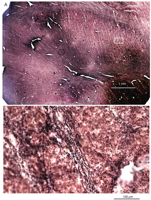
Schmued, L. C. (1990). A rapid, sensitive histochemical stain for myelin in frozen brain sections. Journal of Histochemistry & Cytochemistry,38(5), 717-720.
Are the "bumps" in any way "analogous" to the "brain warts" seen in entorhinal areas of some human brains (G. W. van Hoesen and A. Solodkin (1993)?
Comment: We think this is a similar phenomenon.
Change: We included the Hoesen and A. Solodkin (1993) reference in our discussion.
At least slightly more background (ie, a separate section or, if necessary, supplement) would be helpful, going into more detail on the several subdivisions of the ION and if these undergo major alterations in the elephant.
Comment: The strength of the paper is the detailed delineation of the trunk module, based on myelin stripes and isomorphism. We don’t think we have strong evidence on ION subdivisions, because it appears the trigeminal tract cannot be easily traced in elephants. Accordingly, we find it difficult to add information here.
Change: None.
Is there evidence from the literature of other conspicuous gross anatomical translocations, in any species, especially in subcortical regions?
Comment: The best example that comes to mind is the star-nosed mole brainstem. There is a beautiful paper comparing the star-nosed mole brainstem to the normal mole brainstem (Catania et al 2011). The principal trigeminal nucleus in the star-nosed mole is far more rostral and also more medial than in the mole; still, such rearrangements are minor compared to what we propose in elephants.
Catania, Kenneth C., Duncan B. Leitch, and Danielle Gauthier. "A star in the brainstem reveals the first step of cortical magnification." PloS one 6.7 (2011): e22406.
Change: None.
(3) A major point concerns the isomorphism between the putative trigeminal nuclei and the trunk specialization. I think this can be much better presented, at least with more discussion and other examples. The Authors mention about the rodent "barrels," but it seemed strange to me that they do not refer to their own results in pig (C. Ritter et al., 2023) nor the work from Ken Catania, 2002 (star-nosed mole; "fingerprints in the brain") or other that might be appropriate. I concur with the Reviewer that there should be more comparative data.
Comment: We agree.
Change: We added a discussion of other isomorphisms including the the star-nosed mole to our paper.
(4) Textual organization could be improved.
The Abstract all-important Introduction is a longish, semi "run-on" paragraph. At a minimum this should be broken up. The last paragraph of the Introduction puts forth five issues, but these are only loosely followed in the Results section. I think clarity and good organization is of the upmost importance in this manuscript. I recommend that the Authors begin the Results with a section on the trunk folds (currently figure 5, and discussion), continue with the several points related to the identification of the trigeminal nuclei, and continue with a parallel description of ION with more parallel data on the putative trigeminal and IO structures (currently referee Table 1, but incorporate into the text and add higher magnification of nucleus-specific cell types in the IO and trigeminal nuclei). Relevant comparative data should be included in the Discussion.
Comment: 1. We agree with the referee that our abstract needed to be revised. 2. We also think that our ms was heavily altered by the insertion of the new Figure 2, which complemented Figure 1 from our first submission and is concerned with the identification of the inferior olive. From a standpoint of textual flow such changes were not ideal, but the revisions massively added to the certainty with which we identify the trigeminal nuclei. Thus, although we are not as content as we were with the flow, we think the ms advanced in the revision process and we would like to keep the Figure sequence as is. 3. We already noted above that we included additional comparative evidence.
Change: 1. We revised our abstract. 2. We added comparative evidence.
Reviewer #5 (Recommendations For The Authors):
The data is invaluable and provides insights into some of the largest mammals on the planet.
Comment: We are incredibly thankful for this positive assessment.
Reviewer #2 (Public Review):
Here I submit my previous review and a great deal of additional information following on from the initial review and the response by the authors.
* Initial Review *
Assessment:
This manuscript is based upon the unprecedented identification of an apparently highly unusual trigeminal nuclear organization within the elephant brainstem, related to a large trigeminal nerve in these animals. The apparently highly specialized elephant trigeminal nuclear complex identified in the current study has been classified as the inferior olivary nuclear complex in four previous studies of the elephant brainstem. The entire study is predicated upon the correct identification of the trigeminal sensory nuclear complex and the inferior olivary nuclear complex in the elephant, and if this is incorrect, then the remainder of the manuscript is merely unsupported speculation. There are many reasons indicating that the trigeminal nuclear complex is misidentified in the current study, rendering the entire study, and associated speculation, inadequate at best, and damaging in terms of understanding elephant brains and behaviour at worst.
Original Public Review:
The authors describe what they assert to be a very unusual trigeminal nuclear complex in the brainstem of elephants, and based on this, follow with many speculations about how the trigeminal nuclear complex, as identified by them, might be organized in terms of the sensory capacity of the elephant trunk.<br /> The identification of the trigeminal nuclear complex/inferior olivary nuclear complex in the elephant brainstem is the central pillar of this manuscript from which everything else follows, and if this is incorrect, then the entire manuscript fails, and all the associated speculations become completely unsupported.
The authors note that what they identify as the trigeminal nuclear complex has been identified as the inferior olivary nuclear complex by other authors, citing Shoshani et al. (2006; 10.1016/j.brainresbull.2006.03.016) and Maseko et al (2013; 10.1159/000352004), but fail to cite either Verhaart and Kramer (1958; PMID 13841799) or Verhaart (1962; 10.1515/9783112519882-001). These four studies are in agreement, but the current study differs.
Let's assume for the moment that the four previous studies are all incorrect and the current study is correct. This would mean that the entire architecture and organization of the elephant brainstem is significantly rearranged in comparison to ALL other mammals, including humans, previously studied (e.g. Kappers et al. 1965, The Comparative Anatomy of the Nervous System of Vertebrates, Including Man, Volume 1 pp. 668-695) and the closely related manatee (10.1002/ar.20573). This rearrangement necessitates that the trigeminal nuclei would have had to "migrate" and shorten rostrocaudally, specifically and only, from the lateral aspect of the brainstem where these nuclei extend from the pons through to the cervical spinal cord (e.g. the Paxinos and Watson rat brain atlases), the to the spatially restricted ventromedial region of specifically and only the rostral medulla oblongata. According to the current paper the inferior olivary complex of the elephant is very small and located lateral to their trigeminal nuclear complex, and the region from where the trigeminal nuclei are located by others appears to be just "lateral nuclei" with no suggestion of what might be there instead.
Such an extraordinary rearrangement of brainstem nuclei would require a major transformation in the manner in which the mutations, patterning, and expression of genes and associated molecules during development occur. Such a major change is likely to lead to lethal phenotypes, making such a transformation extremely unlikely. Variations in mammalian brainstem anatomy are most commonly associated with quantitative changes rather than qualitative changes (10.1016/B978-0-12-804042-3.00045-2).
The impetus for the identification of the unusual brainstem trigeminal nuclei in the current study rests upon a previous study from the same laboratory (10.1016/j.cub.2021.12.051) that estimated that the number of axons contained in the infraorbital branch of the trigeminal nerve that innervate the sensory surfaces of the trunk is approximately 400 000. Is this number unusual? In a much smaller mammal with a highly specialized trigeminal system, the platypus, the number of axons innervating the sensory surface of the platypus bill skin comes to 1 344 000 (10.1159/000113185). Yet, there is no complex rearrangement of the brainstem trigeminal nuclei in the brain of the developing or adult platypus (Ashwell, 2013, Neurobiology of Monotremes), despite the brainstem trigeminal nuclei being very large in the platypus (10.1159/000067195). Even in other large-brained mammals, such as large whales that do not have a trunk, the number of axons in the trigeminal nerve ranges between 400,000 and 500,000 (10.1007/978-3-319-47829-6_988-1). The lack of comparative support for the argument forwarded in the previous and current study from this laboratory, and that the comparative data indicates that the brainstem nuclei do not change in the manner suggested in the elephant, argues against the identification of the trigeminal nuclei as outlined in the current study. Moreover, the comparative studies undermine the prior claim of the authors, informing the current study, that "the elephant trigeminal ganglion ... point to a high degree of tactile specialization in elephants" (10.1016/j.cub.2021.12.051). While clearly the elephant has tactile sensitivity in the trunk, it is questionable as to whether what has been observed in elephants is indeed "truly extraordinary".
But let's look more specifically at the justification outlined in the current study to support their identification of the unusually located trigeminal sensory nuclei of the brainstem.
(1) Intense cytochrome oxidase reactivity<br /> (2) Large size of the putative trunk module<br /> (3) Elongation of the putative trunk module<br /> (4) Arrangement of these putative modules correspond to elephant head anatomy<br /> (5) Myelin stripes within the putative trunk module that apparently match trunk folds<br /> (6) Location apparently matches other mammals<br /> (7) Repetitive modular organization apparently similar to other mammals.<br /> (8) The inferior olive described by other authors lacks the lamellated appearance of this structure in other mammals
Let's examine these justifications more closely.
(1) Cytochrome oxidase histochemistry is typically used as an indicative marker of neuronal energy metabolism. The authors indicate, based on the "truly extraordinary" somatosensory capacities of the elephant trunk, that any nuclei processing this tactile information should be highly metabolically active, and thus should react intensely when stained for cytochrome oxidase. We are told in the methods section that the protocols used are described by Purkart et al (2022) and Kaufmann et al (2022). In neither of these cited papers is there any description, nor mention, of the cytochrome oxidase histochemistry methodology, thus we have no idea of how this histochemical staining was done. In order to obtain the best results for cytochrome oxidase histochemistry, the tissue is either processed very rapidly after buffer perfusion to remove blood or in recently perfusion-fixed tissue (e.g., 10.1016/0165-0270(93)90122-8). Given: (1) the presumably long post-mortem interval between death and fixation - "it often takes days to dissect elephants"; (2) subsequent fixation of the brains in 4% paraformaldehyde for "several weeks"; (3) The intense cytochrome oxidase reactivity in the inferior olivary complex of the laboratory rat (Gonzalez-Lima, 1998, Cytochrome oxidase in neuronal metabolism and Alzheimer's diseases); and (4) The lack of any comparative images from other stained portions of the elephant brainstem; it is difficult to support the justification as forwarded by the authors. It is likely that the histochemical staining observed is background reactivity from the use of diaminobenzidine in the staining protocol. Thus, this first justification is unsupported.<br /> Justifications (2), (3), and (4) are sequelae from justification (1). In this sense, they do not count as justifications, but rather unsupported extensions.
(4) and (5) These are interesting justifications, as the paper has clear internal contradictions, and (5) is a sequelae of (4). The reader is led to the concept that the myelin tracts divide the nuclei into sub-modules that match the folding of the skin on the elephant trunk. One would then readily presume that these myelin tracts are in the incoming sensory axons from the trigeminal nerve. However, the authors note that this is not the case: "Our observations on trunk module myelin stripes are at odds with this view of myelin. Specifically, myelin stripes show no tapering (which we would expect if axons divert off into the tissue). More than that, there is no correlation between myelin stripe thickness (which presumably correlates with axon numbers) and trigeminal module neuron numbers. Thus, there are numerous myelinated axons, where we observe few or no trigeminal neurons. These observations are incompatible with the idea that myelin stripes form an axonal 'supply' system or that their prime function is to connect neurons. What do myelin stripe axons do, if they do not connect neurons? We suggest that myelin stripes serve to separate rather than connect neurons." So, we are left with the observation that the myelin stripes do not pass afferent trigeminal sensory information from the "truly extraordinary" trunk skin somatic sensory system, and rather function as units that separate neurons - but to what end? It appears that the myelin stripes are more likely to be efferent axonal bundles leaving the nuclei (to form the olivocerebellar tract). This justification is unsupported.
(6) The authors indicate that the location of these nuclei matches that of the trigeminal nuclei in other mammals. This is not supported in any way. In ALL other mammals in which the trigeminal nuclei of the brainstem have been reported they are found in the lateral aspect of the brainstem, bordered laterally by the spinal trigeminal tract. This is most readily seen and accessible in the Paxinos and Watson rat brain atlases. The authors indicate that the trigeminal nuclei are medial to the facial nerve nucleus, but in every other species, the trigeminal sensory nuclei are found lateral to the facial nerve nucleus. This is most salient when examining a close relative, the manatee (10.1002/ar.20573), where the location of the inferior olive and the trigeminal nuclei matches that described by Maseko et al (2013) for the African elephant. This justification is not supported.
(7) The dual to quadruple repetition of rostro-caudal modules within the putative trigeminal nucleus as identified by the authors relies on the fact that in the neurotypical mammal, there are several trigeminal sensory nuclei arranged in a column running from the pons to the cervical spinal cord, these include (nomenclature from Paxinos and Watson in roughly rostral to caudal order) the Pr5VL, Pr5DM, Sp5O, Sp5I, and Sp5C. But, these nuclei are all located far from the midline and lateral to the facial nerve nucleus, unlike what the authors describe in the elephants. These rostrocaudal modules are expanded upon in Figure 2, and it is apparent from what is shown that the authors are attributing other brainstem nuclei to the putative trigeminal nuclei to confirm their conclusion. For example, what they identify as the inferior olive in figure 2D is likely the lateral reticular nucleus as identified by Maseko et al (2013). This justification is not supported.
(8) In primates and related species, there is a distinct banded appearance of the inferior olive, but what has been termed the inferior olive in the elephant by other authors does not have this appearance, rather, and specifically, the largest nuclear mass in the region (termed the principal nucleus of the inferior olive by Maseko et al, 2013, but Pr5, the principal trigeminal nucleus in the current paper) overshadows the partial banded appearance of the remaining nuclei in the region (but also drawn by the authors of the current paper). Thus, what is at debate here is whether the principal nucleus of the inferior olive can take on a nuclear shape rather than evince a banded appearance. The authors of this paper use this variance as justification that this cluster of nuclei could not possibly be the inferior olive. Such a "semi-nuclear/banded" arrangement of the inferior olive is seen in, for example, giraffe (10.1016/j.jchemneu.2007.05.003), domestic dog, polar bear, and most specifically the manatee (a close relative of the elephant) (brainmuseum.org; 10.1002/ar.20573). This justification is not supported.
Thus, all the justifications forwarded by the authors are unsupported. Based on methodological concerns, prior comparative mammalian neuroanatomy, and prior studies in the elephant and closely related species, the authors fail to support their notion that what was previously termed the inferior olive in the elephant is actually the trigeminal sensory nuclei. Given this failure, the justifications provided above that are sequelae also fail. In this sense, the entire manuscript and all the sequelae are not supported.
What the authors have not done is to trace the pathway of the large trigeminal nerve in the elephant brainstem, as was done by Maseko et al (2013), which clearly shows the internal pathways of this nerve, from the branch that leads to the fifth mesencephalic nucleus adjacent to the periventricular grey matter, through to the spinal trigeminal tract that extends from the pons to the spinal cord in a manner very similar to all other mammals. Nor have they shown how the supposed trigeminal information reaches the putative trigeminal nuclei in the ventromedial rostral medulla oblongata. These are but two examples of many specific lines of evidence that would be required to support their conclusions. Clearly tract tracing methods, such as cholera toxin tracing of peripheral nerves cannot be done in elephants, thus the neuroanatomy must be done properly and with attention to detail to support the major changes indicated by the authors.
So what are these "bumps" in the elephant brainstem?
Four previous authors indicate that these bumps are the inferior olivary nuclear complex. Can this be supported?
The inferior olivary nuclear complex acts "as a relay station between the spinal cord (n.b. trigeminal input does reach the spinal cord via the spinal trigeminal tract) and the cerebellum, integrating motor and sensory information to provide feedback and training to cerebellar neurons" (https://www.ncbi.nlm.nih.gov/books/NBK542242/). The inferior olivary nuclear complex is located dorsal and medial to the pyramidal tracts (which were not labelled in the current study by the authors but are clearly present in Fig. 1C and 2A) in the ventromedial aspect of the rostral medulla oblongata. This is precisely where previous authors have identified the inferior olivary nuclear complex and what the current authors assign to their putative trigeminal nuclei. The neurons of the inferior olivary nuclei project, via the olivocerebellar tract to the cerebellum to terminate in the climbing fibres of the cerebellar cortex.
Elephants have the largest (relative and absolute) cerebellum of all mammals (10.1002/ar.22425), this cerebellum contains 257 x109 neurons (10.3389/fnana.2014.00046; three times more than the entire human brain, 10.3389/neuro.09.031.2009). Each of these neurons appears to be more structurally complex than the homologous neurons in other mammals (10.1159/000345565; 10.1007/s00429-010-0288-3). In the African elephant, the neurons of the inferior olivary nuclear complex are described by Maseko et al (2013) as being both calbindin and calretinin immunoreactive. Climbing fibres in the cerebellar cortex of the African elephant are clearly calretinin immunopositive and also are likely to contain calbindin (10.1159/000345565). Given this, would it be surprising that the inferior olivary nuclear complex of the elephant is enlarged enough to create a very distinct bump in exactly the same place where these nuclei are identified in other mammals?
What about the myelin stripes? These are most likely to be the origin of the olivocerebellar tract and probably only have a coincidental relationship to the trunk. Thus, given what we know, the inferior olivary nuclear complex as described in other studies, and the putative trigeminal nuclear complex as described in the current study, is the elephant inferior olivary nuclear complex. It is not what the authors believe it to be, and they do not provide any evidence that discounts the previous studies. The authors are quite simply put, wrong. All the speculations that flow from this major neuroanatomical error are therefore science fiction rather than useful additions to the scientific literature.
What do the authors actually have?<br /> The authors have interesting data, based on their Golgi staining and analysis, of the inferior olivary nuclear complex in the elephant.
* Review of Revised Manuscript *
Assessment:
There is a clear dichotomy between the authors and this reviewer regarding the identification of specific structures, namely the inferior olivary nuclear complex and the trigeminal nuclear complex, in the brainstem of the elephant. The authors maintain the position that in the elephant alone, irrespective of all the published data on other mammals and previously published data on the elephant brainstem, these two nuclear complexes are switched in location. The authors maintain that their interpretation is correct, but this reviewer maintains that this interpretation is erroneous. The authors expressed concern that the remainder of the paper was not addressed by the reviewer, but the reviewer maintains that these sequelae to the misidentification of nuclear complexes in the elephant brainstem render any of these speculations irrelevant as the critical structures are incorrectly identified. It is this reviewer's opinion that this paper is incorrect. I provide a lot of detail below in order to provide support to the opinion I express.
Public Review of Current Submission:
As indicated in my previous review of this manuscript (see above), it is my opinion that the authors have misidentified, and indeed switched, the inferior olivary nuclear complex (IO) and the trigeminal nuclear complex (Vsens). It is this specific point only that I will address in this second review, as this is the crucial aspect of this paper - if the identification of these nuclear complexes in the elephant brainstem by the authors is incorrect, the remainder of the paper does not have any scientific validity.
The authors, in their response to my initial review, claim that I "bend" the comparative evidence against them. They further claim that as all other mammalian species exhibit a "serrated" appearance of the inferior olive, and as the elephant does not exhibit this appearance, what was previously identified as the inferior olive is actually the trigeminal nucleus and vice versa.
For convenience, I will refer to IOM and VsensM as the identification of these structures according to Maseko et al (2013) and other authors and will use IOR and VsensR to refer to the identification forwarded in the study under review.<br /> The IOM/VsensR certainly does not have a serrated appearance in elephants. Indeed, from the plates supplied by the authors in response (Referee Fig. 2), the cytochrome oxidase image supplied and the image from Maseko et al (2013) shows a very similar appearance. There is no doubt that the authors are identifying structures that closely correspond to those provided by Maseko et al (2013). It is solely a contrast in what these nuclear complexes are called and the functional sequelae of the identification of these complexes (are they related to the trunk sensation or movement controlled by the cerebellum?) that is under debate.
Elephants are part of the Afrotheria, thus the most relevant comparative data to resolve this issue will be the identification of these nuclei in other Afrotherian species. Below I provide images of these nuclear complexes, labelled in the standard nomenclature, across several Afrotherian species.
(A) Lesser hedgehog tenrec (Echinops telfairi)
Tenrecs brains are the most intensively studied of the Afrotherian brains, these extensive neuroanatomical studies were undertaken primarily by Heinz Künzle. Below I append images (coronal sections stained with cresol violet) of the IO and Vsens (labelled in the standard mammalian manner) in the lesser hedgehog tenrec. It should be clear that the inferior olive is located in the ventral midline of the rostral medulla oblongata (just like the rat) and that this nucleus is not distinctly serrated. The Vsens is located in the lateral aspect of the medulla skirted laterally by the spinal trigeminal tract (Sp5). These images and the labels indicating structures correlate precisely with that provided by Künzle (1997, 10.1016/S0168- 0102(97)00034-5), see his Figure 1K,L. Thus, in the first case of a related species, there is no serrated appearance of the inferior olive, the location of the inferior olive is confirmed through connectivity with the superior colliculus (a standard connection in mammals) by Künzle (1997), and the location of Vsens is what is considered to be typical for mammals. This is in agreement with the authors, as they propose that ONLY the elephants show the variations they report.
Review image 1.
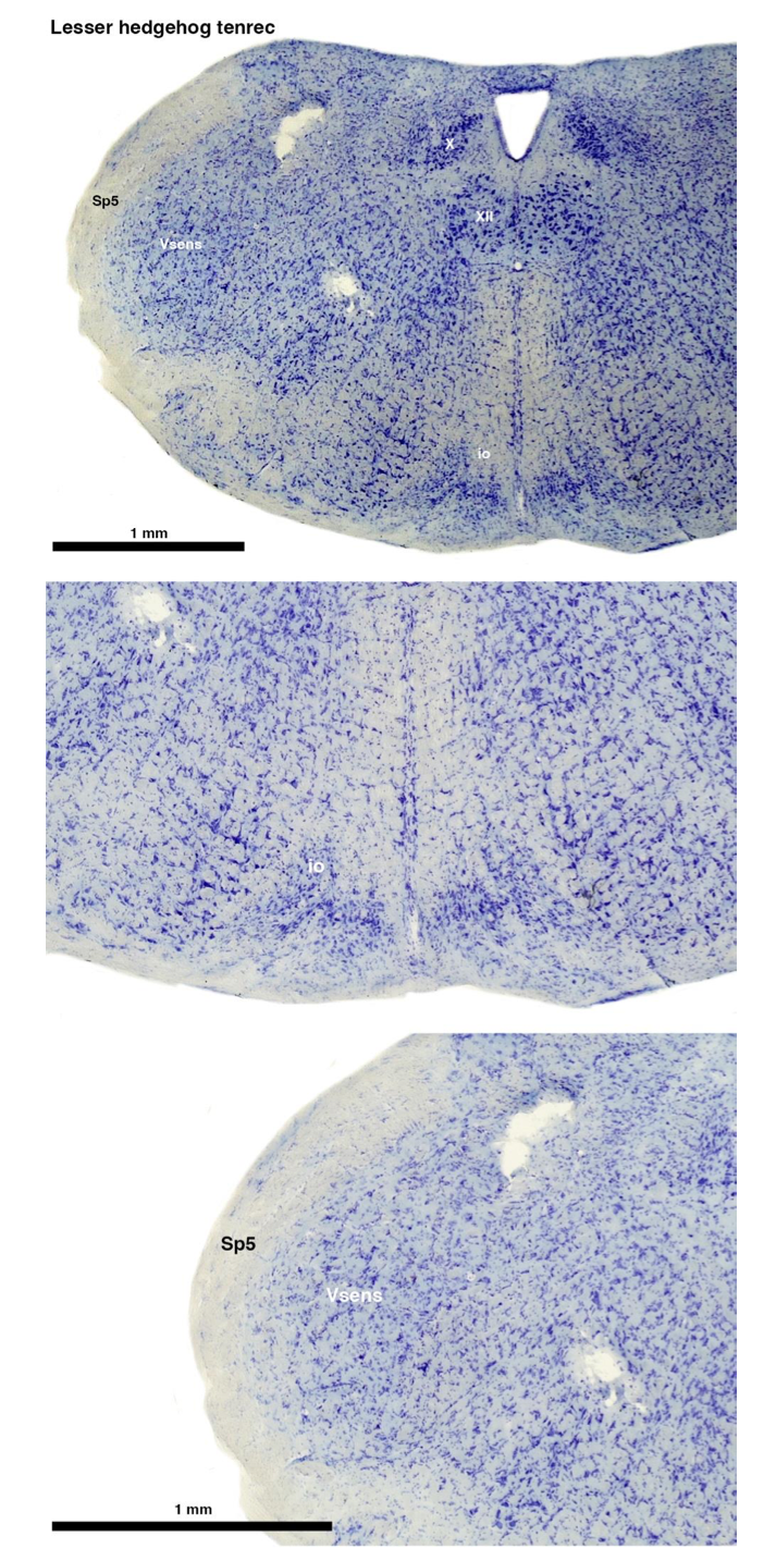
(B) Giant otter shrew (Potomogale velox)
The otter shrews are close relatives of the Tenrecs. Below I append images of cresyl violet (left column) and myelin (right column) stained coronal sections through the brainstem with the IO, Vsens and Sp5 labelled as per standard mammalian anatomy. Here we see hints of the serration of the IO as defined by the authors, but we also see many myelin stripes across the IO. Vsens is located laterally and skirted by the Sp5. This is in agreement with the authors, as they propose that ONLY the elephants show the variations they report.
Review image 2.
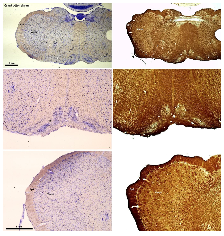
(C) Four-toed sengi (Petrodromus tetradactylus)
The sengis are close relatives of the Tenrecs and otter shrews, these three groups being part of the Afroinsectiphilia, a distinct branch of the Afrotheria. Below I append images of cresyl violet (left column) and myelin (right column) stained coronal sections through the brainstem with the IO, Vsens and Sp5 labelled as per standard mammalian anatomy. Here we see vague hints of the serration of the IO (as defined by the authors), and we also see many myelin stripes across the IO. Vsens is located laterally and skirted by the Sp5. This is in agreement with the authors, as they propose that ONLY the elephants show the variations they report.
Review image 3.
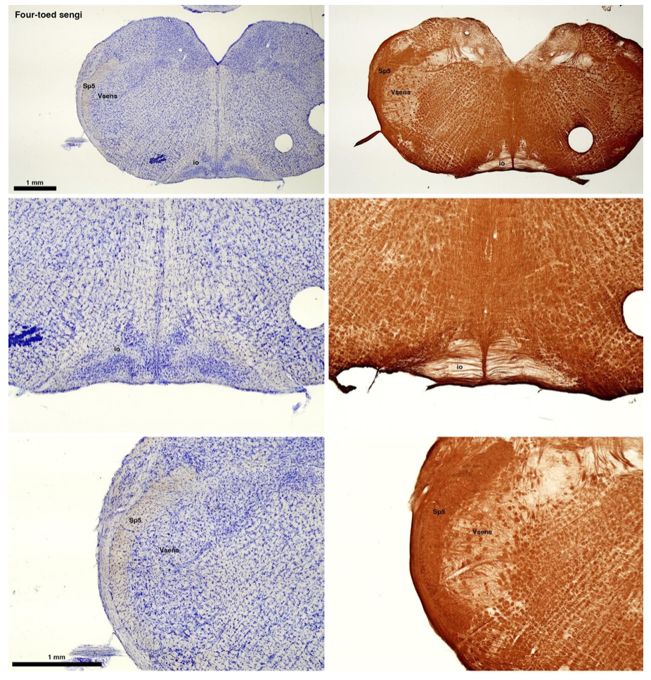
(D) Rock hyrax (Procavia capensis)
The hyraxes, along with the sirens and elephants form the Paenungulata branch of the Afrotheria. Below I append images of cresyl violet (left column) and myelin (right column) stained coronal sections through the brainstem with the IO, Vsens and Sp5 labelled as per the standard mammalian anatomy. Here we see hints of the serration of the IO (as defined by the authors), but we also see evidence of a more "bulbous" appearance of subnuclei of the IO (particularly the principal nucleus), and we also see many myelin stripes across the IO. Vsens is located laterally and skirted by the Sp5. This is in agreement with the authors, as they propose that ONLY the elephants show the variations they report.
Review image 4.
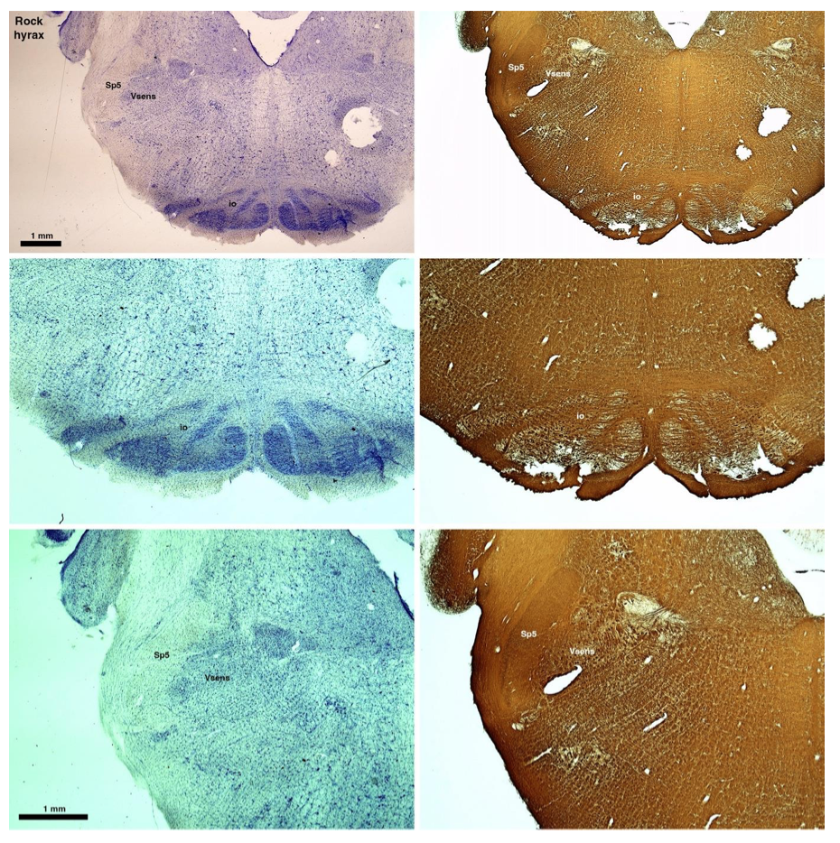
(E) West Indian manatee (Trichechus manatus)
The sirens are the closest extant relatives of the elephants in the Afrotheria. Below I append images of cresyl violet (top) and myelin (bottom) stained coronal sections (taken from the University of Wisconsin-Madison Brain Collection, https://brainmuseum.org, and while quite low in magnification they do reveal the structures under debate) through the brainstem with the IO, Vsens and Sp5 labelled as per standard mammalian anatomy. Here we see the serration of the IO (as defined by the authors). Vsens is located laterally and skirted by the Sp5. This is in agreement with the authors, as they propose that ONLY the elephants show the variations they report.
Review image 5.
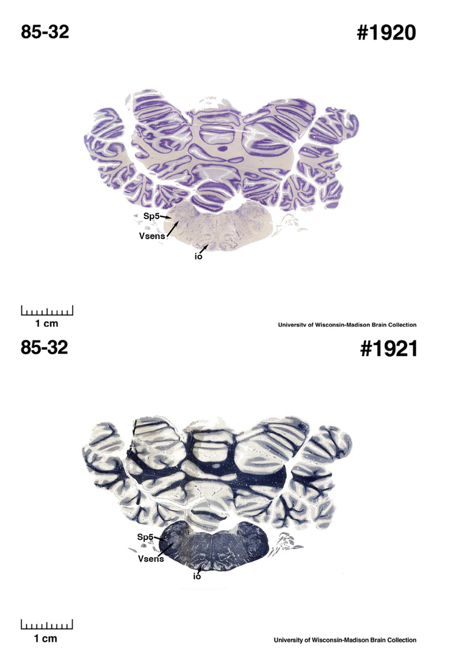
These comparisons and the structural identification, with which the authors agree as they only distinguish the elephants from the other Afrotheria, demonstrate that the appearance of the IO can be quite variable across mammalian species, including those with a close phylogenetic affinity to the elephants. Not all mammal species possess a "serrated" appearance of the IO. Thus, it is more than just theoretically possible that the IO of the elephant appears as described prior to this study.
So what about elephants? Below I append a series of images from coronal sections through the African elephant brainstem stained for Nissl, myelin, and immunostained for calretinin. These sections are labelled according to standard mammalian nomenclature. In these complete sections of the elephant brainstem, we do not see a serrated appearance of the IOM (as described previously and in the current study by the authors). Rather the principal nucleus of the IOM appears to be bulbous in nature. In the current study, no image of myelin staining in the IOM/VsensR is provided by the authors. However, in the images I provide, we do see the reported myelin stripes in all stains - agreement between the authors and reviewer on this point. The higher magnification image to the bottom left of the plate shows one of the IOM/VsensR myelin stripes immunostained for calretinin, and within the myelin stripes axons immunopositive for calretinin are seen (labelled with an arrow). The climbing fibres of the elephant cerebellar cortex are similarly calretinin immunopositive (10.1159/000345565). In contrast, although not shown at high magnification, the fibres forming the Sp5 in the elephant (in the Maseko description, unnamed in the description of the authors) show no immunoreactivity to calretinin.
Review image 6.
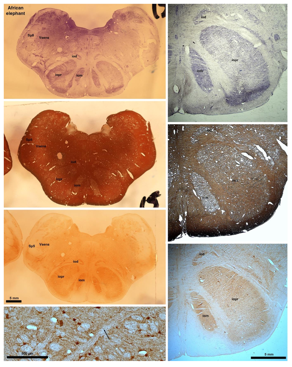
Peripherin Immunostaining
In their revised manuscript the authors present immunostaining of peripherin in the elephant brainstem. This is an important addition (although it does replace the only staining of myelin provided by the authors which is unusual as the word myelin is in the title of the paper) as peripherin is known to specifically label peripheral nerves. In addition, as pointed out by the authors, peripherin also immunostains climbing fibres (Errante et al., 1998). The understanding of this staining is important in determining the identification of the IO and Vsens in the elephant, although it is not ideal for this task as there is some ambiguity. Errante and colleagues (1998; Fig. 1) show that climbing fibres are peripherin-immunopositive in the rat. But what the authors do not evaluate is the extensive peripherin staining in the rat Sp5 in the same paper (Errante et al, 1998, Fig. 2). The image provided by the authors of their peripherin immunostaining (their new Figure 2) shows what I would call the Sp5 of the elephant to be strongly peripherin immunoreactive, just like the rat shown in Errant et al (1998), and moreover in the precise position of the rat Sp5! This makes sense as this is where the axons subserving the "extraordinary" tactile sensitivity of the elephant trunk would be found (in the standard model of mammalian brainstem anatomy). Interestingly, the peripherin immunostaining in the elephant is clearly lamellated...this coincides precisely with the description of the trigeminal sensory nuclei in the elephant by Maskeo et al (2013) as pointed out by the authors in their rebuttal. Errante et al (1998) also point out peripherin immunostaining in the inferior olive, but according to the authors this is only "weakly present" in the elephant IOM/VsensR. This latter point is crucial. Surely if the elephant has an extraordinary sensory innervation from the trunk, with 400,000 axons entering the brain, the VsensR/IOM should be highly peripherin-immunopositive, including the myelinated axon bundles?! In this sense, the authors argue against their own interpretation - either the elephant trunk is not a highly sensitive tactile organ, or the VsensR is not the trigeminal nuclei it is supposed to be.
Summary:
(1) Comparative data of species closely related to elephants (Afrotherians) demonstrates that not all mammals exhibit the "serrated" appearance of the principal nucleus of the inferior olive.
(2) The location of the IO and Vsens as reported in the current study (IOR and VsensR) would require a significant, and unprecedented, rearrangement of the brainstem in the elephants independently. I argue that the underlying molecular and genetic changes required to achieve this would be so extreme that it would lead to lethal phenotypes. Arguing that the "switcheroo" of the IO and Vsens does occur in the elephant (and no other mammals) and thus doesn't lead to lethal phenotypes is a circular argument that cannot be substantiated.
(3) Myelin stripes in the subnuclei of the inferior olivary nuclear complex are seen across all related mammals as shown above. Thus, the observation made in the elephant by the authors in what they call the VsensR, is similar to that seen in the IO of related mammals, especially when the IO takes on a more bulbous appearance. These myelin stripes are the origin of the olivocerebellar pathway and are indeed calretinin immunopositive in the elephant as I show.
(4) What the authors see aligns perfectly with what has been described previously, the only difference being the names that nuclear complexes are being called. But identifying these nuclei is important, as any functional sequelae, as extensively discussed by the authors, is entirely dependent upon accurately identifying these nuclei.
(4) The peripherin immunostaining scores an own goal - if peripherin is marking peripheral nerves (as the authors and I believe it is), then why is the VsensR/IOM only "weakly positive" for this stain? This either means that the "extraordinary" tactile sensitivity of the elephant trunk is non-existent, or that the authors have misinterpreted this staining. That there is extensive staining in the fibre pathway dorsal and lateral to the IOR (which I call the spinal trigeminal tract), supports the idea that the authors have misinterpreted their peripherin immunostaining.
(5) Evolutionary expediency. The authors argue that what they report is an expedient way in which to modify the organisation of the brainstem in the elephant to accommodate the "extraordinary" tactile sensitivity. I disagree. As pointed out in my first review, the elephant cerebellum is very large and comprised of huge numbers of morphologically complex neurons. The inferior olivary nuclei in all mammals studied in detail to date, give rise to the climbing fibres that terminate on the Purkinje cells of the cerebellar cortex. It is more parsimonious to argue that, in alignment with the expansion of the elephant cerebellum (for motor control of the trunk), the inferior olivary nuclei (specifically the principal nucleus) have had additional neurons added to accommodate this cerebellar expansion. Such an addition of neurons to the principal nucleus of the inferior olive could readily lead to the loss of the serrated appearance of the principal nucleus of the inferior olive and would require far less modifications in the developmental genetic program that forms these nuclei. This type of quantitative change appears to be the primary way in which structures are altered in the mammalian brainstem.
Author response:
The following is the authors’ response to the previous reviews.
Public Reviews
Reviewer #1 (Public Review):
Comment: The fact that there are Arid1a transcripts that escape the Cre system in the Arid1a KO mouse model might difficult the interpretation of the data. The phenotype of the Arid1a knockout is probably masked by the fact that many of the sequencing techniques used here are done on a heterogeneous population of knockout and wild type spermatocytes. In relation to this, I think that the use of the term "pachytene arrest" might be overstated, since this is not the phenotype truly observed. Knockout mice produce sperm, and probably litters, although a full description of the subfertility phenotype is lacking, along with identification of the stage at which cell death is happening by detection of apoptosis.
Response: As the reviewer indicates, we did not observe a complete arrest at Pachynema. In fact, the histology shows the presence of spermatids and sperm in seminiferous tubules and epididymides (Fig. Sup. 3). However, our data argue that the wild-type haploid gametes produced were derived from spermatocyte precursors that have likely escaped Cre mediated activity (Fig. Sup. 4). Furthermore, diplotene and metaphase-I spermatocytes lacking ARID1A protein by IF were undetectable in the Arid1acKO testes (Fig. S4B). Therefore, although we do not demonstrate a strict pachytene arrest, it is reasonable to conclude that ARID1A is necessary to progress beyond pachynema. We have revised the manuscript to reflect this point (Abstract lines 17,18; Results lines 153,154)
Comment: It is clear from this work that ARID1a is part of the protein network that contributes to silencing of the sex chromosomes. However, it is challenging to understand the timing of the role of ARID1a in the context of the well-known DDR pathways that have been described for MSCI.
Response: With respect to the comment on the lack of clarity as to which stage of meiosis we observe cell death, our data do suggest that it is reasonable to conclude that mutant spermatocytes (ARID1A-) undergo cell death at pachynema given their inability to execute MSCI, which is a well-established phenotype.
Comment: Staining of chromosome spreads with Arid1a antibody showed localization at the sex chromosomes by diplonema; however, analysis of gene expression in Arid1a KO was performed on pachytene spermatocytes. Therefore, is not very clear how the chromatin remodeling activity of Arid1a in diplonema is affecting gene expression of a previous stage. CUTnRUN showed that ARID1a is present at the sex chromatin in earlier stages, leading to hypothesize that immunofluorescence with ARID1a antibody might not reflect ARID1a real localization.
Response: It is unclear what the reviewer means about not understanding how ARID1A activity at diplonema affects gene expression at earlier stages. Our interpretations were not based solely on the observation of ARID1A associations with the XY body at diplonema. In fact, mRNA expression and CUT&RUN analyses were performed on pachytene-enriched populations. ARID1A's association with the XY body is not exclusive to diplonema. Based on both CUT&RUN and IF data, ARID1A associates with XY chromatin as early as pachynema. Only at late diplonema did we observe ARID1A hyperaccumulation on the XY body by IF.
Reviewer #2 (Public Review):
Comment: The inefficient deletion of ARID1A in this mouse model does not allow any detailed analysis in a quantitative manner.
Response: As explained in our response to these comments in the first revision, we respectfully disagree with this reviewer’s conclusions. We have been quantitative by co-staining for ARID1A, ensuring that we can score mutant pachytene spermatocytes from escapers. Additionally, we provide data to show the efficiency of ARID1A loss in the purified pachytene populations sampled in our genomic assays.
Reviewer #3 (Public Review):
Comment: The data demonstrate that the mutant cells fail to progress past pachytene, although it is unclear whether this specifically reflects pachytene arrest, as accumulation in other stages of Prophase also is suggested by the data in Table 1. The western blot showing ARID1A expression in WT vs. cKO spermatocytes (Fig. S2) is supportive of the cKO model but raises some questions. The blot shows many bands that are at lower intensity in the cKO, at MWs from 100-250kDa. The text and accompanying figure legend have limited information. Are the various bands with reduced expression different isoforms of ARID1A, or something else? What is the loading control 'NCL'? How was quantification done given the variation in signal across a large range of MWs?
Response: The loading control is Nucleolin. With respect to the other bands in the range of 100-250 kDa, it is difficult to say whether they represent ARID1A isoforms. The Uniprot entry for Mouse ARID1A only indicates a large mol. wt sequence of ~242 kDa; therefore, the band corresponding to that size was quantified. There is no evidence to suggest that lower molecular weight isoforms may be translated. Although speculative, it is possible that the lower molecular weight bands represent proteolytic/proteasomal degradation products or products of antibody non-specificity. These points are addressed in the revised manuscript (Legend to Fig S2, lines 926-931). Blots were scanned on a LI-COR Odyssey CLx imager and viewed and quantified using Image Studio Version 5.2.5 (Methods, lines 640-642).
Comment: An additional weakness relates to how the authors describe the relationship between ARID1A and DNA damage response (DDR) signaling. The authors don't see defects in a few DDR markers in ARID1A CKO cells (including a low-resolution assessment of ATR), suggesting that ARID1A may not be required for meiotic DDR signaling. However, as previously noted the data do not rule out the possibility that ARID1A is downstream of DDR signaling and the authors even indicate that "it is reasonable to hypothesize that DDR signaling might recruit BAF-A to the sex chromosomes (lines 509-510)." It therefore is difficult to understand why the authors continue to state that "...the mechanisms underlying ARID1A-mediated repression of the sex-linked transcription are mutually exclusive to DDR pathways regulating sex body formation" (p. 8) and that "BAF-A-mediated transcriptional repression of the sex chromosomes occurs independently of DDR signaling" (p. 16). The data provided do not justify these conclusions, as a role for DDR signaling upstream of ARID1A would mean that these mechanisms are not mutually exclusive or independent of one another.
Response: The reviewer’s argument is reasonable, and we have made the recommended changes (Results, lines 212-215; Discussion, lines 499-500).
Comment: A final comment relates to the impacts of ARID1A loss on DMC1 focus formation and the interesting observation of reduced sex chromosome association by DMC1. The authors additionally assess the related recombinase RAD51 and suggest that it is unaffected by ARID1A loss. However, only a single image of RAD51 staining in the cKO is provided (Fig. S11) and there are no associated quantitative data provided. The data are suggestive but it would be appropriate to add a qualifier to the conclusion regarding RAD51 in the discussion which states that "...loss of ARID1a decreases DMC1 foci on the XY chromosomes without affecting RAD51" given that the provided RAD51 data are not rigorous. In the long-term it also would be interesting to quantitatively examine DMC1 and RAD51 focus formation on autosomes as well.
Response: We agree with the reviewer’s comment and have made the recommended changes (Discussion, lines 518-519).
Response to non-public recommendations
Reviewer 2:
Comment: Meiotic arrest is usually judged based on testicular phenotypes. If mutant testes do not have any haploid spermatids, we can conclude that meiotic arrest is a phenotype. In this case, mutant testes have haploid spermatids and are fertile. The authors cannot conclude meiotic arrest. The mutant cells appear to undergo cell death in the pachytene stage, but the authors cannot say "meiotic arrest."
Response: We disagree with this comment. By IF, we see that ~70% of the spermatocytes have deleted ARID1A. Furthermore, we never observed diplotene spermatocytes that lacked ARID1A. The conclusion that the absence of ARID1A results in a pachynema arrest and that the escapers produce the haploid spermatids is firm.
Comment: Fig. S2 and S3 have wrong figure legends.
Response: The figure legends for Fig. S2 and S3 are correct.
Comment: The authors do not appear to evaluate independent mice for scoring (the result is about 74% deletion above, Table S1). Sup S2: how many independent mice did the authors examine?
Response:These were Sta-Put purified fractions obtained from 14-15 WT and mutant mice. It is difficult to isolate pachytene spermatocytes by Sta-Put at the required purity in sufficient yields using one mouse at a time. We used three technical replicates to quantify the band intensity, and the error bars represent the standard error of the mean (S.E.M) of the band intensity.
Comment: Comparison of cKO and wild-type littermate yielded nearly identical results (Avg total conc WT = 32.65 M/m; Avg total conc cKO = 32.06 M/ml)". This sounds like a negative result (i.e., no difference between WT and cKO).
Response: This is correct. There is no difference between Arid1aWT and Arid1aCKO sperm production. This is because wild-type haploid gametes produced were derived from spermatocyte precursors that have escaped Cre-mediated activity (Fig. S4). These data merely serve to highlight an inherent caveat of our conditional knockout model and are not intended to support the main conclusion that ARID1A is necessary for pachytene progression.
Comment: The authors now admit ~ 70 % efficiency in deletion, and the authors did not show the purity of these samples. If the purity of pachytene spermatocytes is ~ 80%, the real proportion of mutant cells can be ~ 56%. It is very difficult to interpret the data.
Response: The original submission did refer to inefficient Cre-induced recombination. The reviewer asked for the % efficiency, which was provided in the revised version. Also, please refer to Fig. S2, where Western blot analysis demonstrates a significant loss of ARID1A protein levels in CKO relative to WT pachytene spermatocyte populations that were used for CUT&RUN data generation.
Comment: The authors should not use the other study to justify their own data. The H3.3 ChIP-seq data in the NAR paper detected clear peaks on autosomes. However, in this study, as shown in Fig. S7A, the authors detected only 4 peaks on autosomes based on MACS2 peak calling. This must be a failed experiment. Also, S7A appears to have labeling errors.
Response: I believe the reviewer is referring to supplementary figure 8A. Here, it is not clear which labeling errors the reviewer is referring to. In the wild type, the identified peaks were overwhelmingly sex-linked intergenic sites. This is consistent with the fact that H3.3 is hyper-accumulated on the sex chromosomes at pachynema.
The authors of the NAR paper did not perform a peak-calling analysis using MACS2 or any other peak-calling algorithm. They merely compared the coverage of H3.3 relative to input. Therefore, it is not clear on what basis the reviewer says that the NAR paper identified autosomal peaks. Their H3.3 signal appears widely distributed over a 6 kb window centered at the TSS of autosomal genes, which, compared to input, appears enriched. Our data clearly demonstrates a less noisy and narrower window of H3.3 enrichment at autosomal TSSs in WT pachytene spermatocytes, albeit at levels lower than that seen in CKO pachytene spermatocytes (Fig S8B and see data copied below for each individual replicate). Moreover, the lack of peaks does not mean that there was an absence of H3.3 at these autosomal TSSs (Supp. Fig. S8B). Therefore, we disagree with the reviewer’s comment that the H3.3 CUT&RUN was a failed experiment.
Author response image 1.
H3.3 Occupancy at genes mis-regulated in the absence of ARID1A
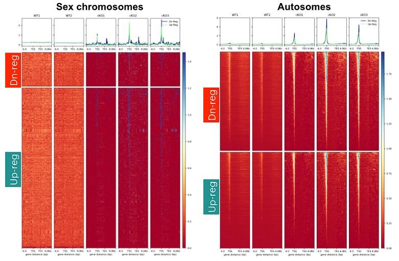
Comment: If the author wishes to study the function of ARID2 in spermatogenesis, they may need to try other cre-lines to have more robust phenotypes, and all analyses must be redone using a mouse model with efficient deletion of ARID2.
Response: As noted, we chose Stra8-Cre to conditionally knockout Arid1a because ARID1A is haploinsufficient during embryonic development. The lack of Cre expression in the maternal germline allows for transmission of the floxed allele, allowing for the experiments to progress.
Comment: The inefficient deletion of ARID1A in this mouse model does not allow any detailed analysis in a quantitative manner.
Response: In many experiments, we have been quantitative when possible by co-staining for ARID1A, ensuring that we can score mutant pachytene spermatocytes from escapers. Additionally, we provide data to show the efficiency of ARID1A loss in the purified pachytene populations sampled in our genomic assays.
Reviewer 3:
Comment: The Methods section refers to antibodies as being in Supplementary Table 3, but the table is labeled as Supplementary Table 2.
Response: This has been corrected
Author response:
The following is the authors’ response to the previous reviews.
Public Reviews:
Reviewer #1 (Public Review):
Although this manuscript contains a potentially interesting piece of work that delineates a mechanism of IQCH that associates with spermatogenesis, this reviewer feels that a number of issues require clarification and re-evaluation for a better understanding of the role of IQCH in spermatogenesis. With the shortage of logics and supporting data, causal relationships are still not clear among IQCH, CaM, and HNRPAB. The most serious point in this manuscript could be that the authors try to generalize their interpretations with too simplified model from limited pieces of their data. The way the data and the logic are presented needs to be largely revised, and several interpretations should be supported by direct evidence.
Response: Thank you for the reviewer’s comment. IQCH is a calmodulin-binding protein, and the binding of IQCH and CaM was confirmed by LC-MS/MS analysis and co-IP assay using sperm lysate. We thus speculated that if the interaction of IQCH and CaM might be a prerequisite for IQCH function. To prove that speculation, we took HNRPAB as an example. We knocked down IQCH in cultured cells, and a decrease in the expression of HNRPAB was observed. Similarly, when we knocked down CaM in cultured cells, and a decrease in the expression of HNRPAB was also detected. However, these results cannot exclude that IQCH or CaM could regulate HNRPAB expression alone. To investigate that if IQCH or CaM could regulate HNRPAB expression alone, we overexpressed IQCH in cells that knocked down CaM, while the expression of HNRPAB cannot be rescued, suggesting that IQCH cannot regulate HNRPAB expression when CaM is reduced. In consistent, we overexpressed CaM in cells that knocked down IQCH, while the expression of HNRPAB cannot be rescued, suggesting that CaM cannot regulate HNRPAB expression when IQCH is reduced. Thus, IQCH or CaM cannot regulate HNRPAB expression alone. Moreover, we deleted the IQ motif of IQCH, which is required for binding to CaM. The co-IP results showed that the interaction of IQCH and CaM was disrupted when deleting the IQ motif of IQCH, and the expression of HNRPAB was decreased. Therefore, we suggested that the interaction of IQCH and CaM might be required for IQCH regulating HNRPAB. In future studies, we will further investigate the relationships among IQCH, CaM, and HNRPAB.
Reviewer #3 (Public Review):
(1) More background details are needed regarding the proteins involved, in particular IQ proteins and calmodulin. The authors state that IQ proteins are not well-represented in the literature, but do not state how many IQ proteins are encoded in the genome. They also do not provide specifics regarding which calmodulins are involved, since there are at least 5 family members in mice and humans. This information could help provide more granular details about the mechanism to the reader and help place the findings in context.
Response: Thanks to reviewer’s suggestion. We have provided additional background information regarding IQ-containing protein family members in humans and mice, as well as other IQ-containing proteins implicated in male fertility, in the Introduction section. Furthermore, we have supplemented the Introduction with background information concerning the association between CaM and male infertility.
(2) The mouse fertility tests could be improved with more depth and rigor. There was no data regarding copulatory plug rate; data was unclear regarding how many WT females were used for the male breeding tests and how many litters were generated; the general methodology used for the breeding tests in the Methods section was not very explicitly or clearly described; the sample size of n=3 for the male breeding tests is rather small for that type of assay; and, given that ICHQ appears to be expressed in testicular interstitial cells (Fig. S10) and somewhat in other organs (Fig. S2), another important parameter of male fertility that should be addressed is reproductive hormone levels (e.g., LH, FSH, and testosterone). While normal epididymal size in Fig. S3 suggests that hormone (testosterone) levels are normal, epididymal size and/or weight were not rigorously quantified.
Response: Thanks to reviewer’s comment. We have provided the data regarding copulatory plug rate and the average number of litters for breeding tests in revised Figure 3—figure supplement 2. The methodology used for the breeding tests has been revised to be more detailed and explicit in the revised Method section. Moreover, we have increased the sample size for male breeding tests to n=6. We measured the serum levels of FSH, LH, and Testosterone in the WT (9.3±1.9 ng/ml, 0.93±0.15 ng/ml, and 0.2±0.03 ng/ml) and Iqch KO mice (12±2 ng/ml, 1.17±0.2 ng/ml, and 0.2±0.04 ng/ml). There was no significant difference observed in the serum levels of reproductive hormones between WT and Iqch KO mice; therefore, we did not include the data in the study. Furthermore, we have added quantitative data on epididymal size in the revised Figure 3—figure supplement 2.
(3) The Western blots in Figure 6 should be rigorously quantified from multiple independent experiments so that there is stronger evidence supporting claims based on those assays.
Response: We appreciate the reviewer's comment. As suggested, we have added quantified data in Figure 6—figure supplement 2 from the results of Western blotting in Figure 6.
(4) Some of the mouse testis images could be improved. For example, the PNA and PLCz images in Figure S7 are difficult to interpret in that the tubules do not appear to be stage-matched, and since the authors claimed that testicular histology is unaffected in knockout testes, it should be feasible to stage-match control and knockout samples. Also, the anti-ICHQ and CaM immunofluorescence in Figure S10 would benefit from some cell-type-specific co-stains to more rigorously define their expression patterns, and they should also be stage-matched.
Response: Thanks to reviewer’s suggestions. We have included immunofluorescence images of anti-PLCz, anti-PNA and anti-IQCH and CaM during spermatogenesis development.
Recommendations for the authors:
Reviewer #1 (Recommendations For The Authors):
(1) There are multiple grammatical errors and statements drawn beyond the results. The entire manuscript would benefit from professional editing.
Response: We are sorry for the grammatical errors. We have enlisted professional editing services to refine our manuscript.
(2) Line 40, "Firstly" is not appropriate here.
Response: Thanks to reviewer’s comment. The word "Firstly" has been removed from the revised manuscript.
(3) Line 44, "processes".
Response: Thanks to reviewer’s suggestion. We have changed “process” in to “processes” on line 45.
(4) "spermatocytogenesis (mitosis)" is incorrect.
Response: Thanks to reviewer’s comment. We have changed “spermatocytogenesis (mitosis)” in to “mitosis” on line 47.
(5) Ca and Ca2+ are both used in line 67 - 77. Be consistent.
Response: We appreciate the reviewer's detailed checks. We have maintained consistency by revising instances of "Ca" to "Ca2+" in revised manuscript.
(6) Line 238 to 240, "To elucidate the molecular mechanism by which IQCH regulates male fertility, we performed liquid chromatography tandem mass spectrometry (LC-MS/MS) analysis using mouse sperm lysates and detected 288 interactors of IQCH (Data S1)."It is not clear how LC-MS/MS using mouse sperm lysates could detect "288 interactors of IQCH"? A co-IP experiment for IQCH using sperm lysates prior to LC-MS/MS is needed to detect "interactors of IQCH". However, in the Methods section, consistent with the main text, proteomic quantification was conducted for protein extract from sperm. Figure legend for Fig. 5 did not explain this, either.Thus, it is unable to evaluate Figure 5.
Response: We sincerely apologize for the oversight. Following reviewer’s suggestions, we have supplemented the method details of LC-MS/MS experiment in the Methods section of revised manuscript. Additionally, we conducted a co-IP experiment for IQCH using sperm lysates prior to LC-MS/MS and we did not include the corresponding figure in the manuscript. The results are as follows:
Author response image 1.
The results of a co-IP experiment for IQCH using sperm lysates from WT mice.
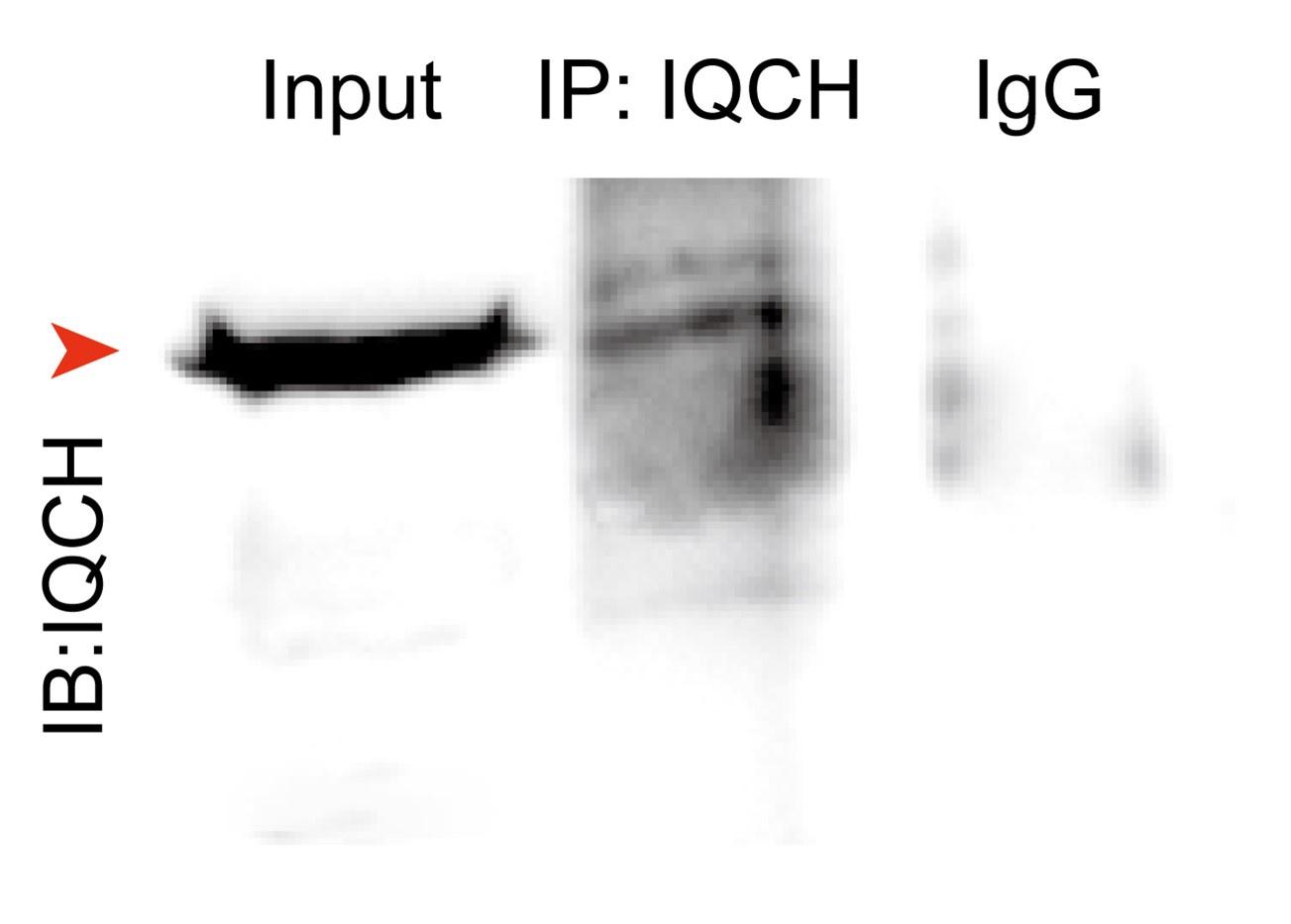
(7) Line 246, "... key proteins that might be activated by IQCH". What does "activated" here refer to? Should it be "upregulated"?
Response: We are sorry to our inexact statement. Instead, "upregulated" would better convey the intended meaning. According to reviewer’s suggestions, we have modified "activated" into "upregulated".
(8) Line 252 to 254, "the cross-analysis revealed that 76 proteins were shared between the IQCH-bound proteins and the IQCH-activated proteins (Fig. 5E), implicating this subset of genes as direct targets." This is a confusing statement. Is the author trying to say, IQCH-bound proteins have upregulated expression, suggesting that IQCH enhances their expression?
Response: We appreciate the reviewer's comment regarding the clarity of the statement in Line 252 to 254 of the manuscript. We have modified this sentence into “Importantly, cross-analysis revealed that 76 proteins were shared between the IQCH-bound proteins and the downregulated proteins in Iqch KO mice (Figure 5E), suggesting that IQCH might regulate their expression by the interaction.”
(9) Line 260 to 261, "SYNCRIP, HNRNPK, FUS, EWSR1, ANXA7, SLC25A4, and HNRPAB ... the loss of which showed the greatest influence on the phenotype of the Iqch KO mice." There is no evidence suggesting that the loss of SYNCRIP, HNRNPK, FUS, EWSR1, ANXA7, SLC25A4, and HNRPAB leads to Iqch KO phenotype.
Response: We apologize for our inaccurate statement. According to the literature, Fus KO, Ewsr1 KO, and Hnrnpk KO male mice were infertile, showing the spermatogenic arrest with absence of spermatozoa (Kuroda et al. 2000; Tian et al. 2021; Xu et al. 2022). Syncrip is involved meiotic process in Drosophila by interacting with Doublefault (Sechi et al. 2019). HNRPAB might be associated with mouse spermatogenesis by binding to Protamine 2 and contributing its translational regulation. Specifically, ANXA7 is a calcium-dependent phospholipid-binding protein that is a negative regulator of mitochondrial apoptosis (Du et al. 2015). Loss of SLC25A4 results in mitochondrial energy metabolism defects in mice (Graham et al. 1997). Moreover, RNA immunoprecipitation on formaldehyde cross-linked sperm followed by qPCR detected the interactions between HNRPAB and Catsper1, Catsper2, Catsper3, Ccdc40, Ccdc39, Ccdc65, Dnah8, Irrc6, and Dnhd1, which are essential for sperm development (Fukuda et al. 2013). Our Iqch KO mice showed abnormal sperm count, motility, morphology, and mitochondria, so we inferenced that IQCH might play a role in spermatogenesis by regulating the expression of SYNCRIP, HNRNPK, FUS, EWSR1, ANXA7, SLC25A4, and HNRPAB to some extent. We have changed an appropriate stamen that “We focused on SYNCRIP, HNRNPK, FUS, EWSR1, ANXA7, SLC25A4, and HNRPAB, which play important roles in spermatogenesis.”
(10) Fig. 6C and 6D use different styles of error bars.
Response: We are sorry for our oversight. In accordance with the reviewer's recommendations, we have modified the representation of error bars in the revised Fig. 6C.
(11) Line 296 to 297, "As expected, CaM interacted with IQCH, as indicated by LC-MS/MS analysis". It is not clear how LC-MS/MS detects protein interaction.
Response: As reviewer’s suggestions, we have supplemented the method details of LC-MS/MS experiment in the Methods section of revised manuscript. The results of proteins interacting with IQCH in sperm lysates from the LC-MS/MS experiment analysis were submitted as Figure 5—source data 1.
(12) It is still not clear how the interaction between IQCH, CaM, and HNRPAB is required for the expression of each other.
Response: Thank you for the reviewer’s comment. IQCH is a calmodulin-binding protein, and the binding of IQCH and CaM was confirmed by LC-MS/MS analysis and co-IP assay using sperm lysate. We thus speculated that if the interaction of IQCH and CaM might be a prerequisite for IQCH function. To prove that speculation, we took HNRPAB as an example. We knocked down IQCH in cultured cells, and a decrease in the expression of HNRPAB was observed. Similarly, when we knocked down CaM in cultured cells, and a decrease in the expression of HNRPAB was also detected. However, these results cannot exclude that IQCH or CaM could regulate HNRPAB expression alone. To investigate that if IQCH or CaM could regulate HNRPAB expression alone, we overexpressed IQCH in cells that knocked down CaM, while the expression of HNRPAB cannot be rescued, suggesting that IQCH cannot regulate HNRPAB expression when CaM is reduced. In consistent, we overexpressed CaM in cells that knocked down IQCH, while the expression of HNRPAB cannot be rescued, suggesting that CaM cannot regulate HNRPAB expression when IQCH is reduced. Thus, IQCH or CaM cannot regulate HNRPAB expression alone. Moreover, we deleted the IQ motif of IQCH, which is required for binding to CaM. The co-IP results showed that the interaction of IQCH and CaM was disrupted when deleting the IQ motif of IQCH, and the expression of HNRPAB was decreased. Therefore, we suggested that the interaction of IQCH and CaM might be required for IQCH regulating HNRPAB. In future studies, we will further investigate the relationships among IQCH, CaM, and HNRPAB.
Reviewer #3 (Recommendations For The Authors):
The authors have addressed my minor concerns. However, they neglected to address any of my more significant concerns in the public review. I assume that they simply overlooked these critiques, despite the fact that eLife explicitly states that "...as a general rule, concerns about a claim not being justified by the data should be explained in the public review." Therefore, the authors should have looked more carefully at the public reviews. As a result, my major concerns about the manuscript remain.
Response: We apologize for overlooking the public review process. We have improved our study based on the feedback received during the public review.
Author response:
The following is the authors’ response to the previous reviews.
Reviewer #1 (Recommendations For The Authors):
The additional data included in this revision nicely strengthens the major claim.
I apologize that my comment about K+ concentration in the prior review was unclear. The cryoEM structure of KCNQ1 with S4 in the resting state was obtained with lowered K+ relative to the active state. Throughout the results and discussion it seems implied that the change in voltage sensor state is somehow causative of the change in selectivity filter state while the paper that identified the structures attributes the change in selectivity filter state not to voltage sensors, but to the change in [K+] between the 2 structures. Unless there is a flaw in my understanding of the conditions in which the selectivity filter structures used in modeling were generated, it seems misleading to ignore the change in [K+] when referring to the activated vs resting or up vs down structures. My understanding is that the closed conformation adopted in the resting/low [K+] is similar to that observed in low [K+] previously and is more commonly associated with [K+]-dependent inactivation, not resulting from voltage sensor deactivation as implied here. The original article presenting the low [K+] structure also suggests this. When discussing conformational changes in the selectivity filter, I strongly suggest referring to these structures as activated/high [K+] vs resting/low [K+] or something similar, as the [K+] concentration is a salient variable.
There seems to be some major confusion here and we will try to explain how we think. Note that in the Mandela and MacKinnon paper, there is no significant difference in the amino acid positions in the selectivity filter between low and high K+ when S4 is in the activated position (See Mandala and Mackinnon, PNAS Suppl. Fig S5 C and D). There are only fewer K+ in the selectivity filter in low K+. So, the structure with the distorted selectivity filter is not due to low K+ by itself. Note that there is no real difference between macroscopic currents recorded in low and high K+ solutions (except what is expected from changes in driving force) for KCNQ1/KCNE1 channels (Larsen et al., Bioph J 2011), suggesting that low K+ do not promote the non-conductive state (Figure 1). We now include a section in the Discussion about high/low K+ in the structures and the absence of effects of K+ on the function of KCNQ1/KCNE1 channels.
Author response image 1.
Macroscopic KCNQ1/KCNE1 currents recorded in different K+ conditions. Note that there is no difference between current recorded in low K+ (2 mM) conditions and high (96 mM) K+ conditions (n=3 oocytes). Currents were normalized in respect to high K+.
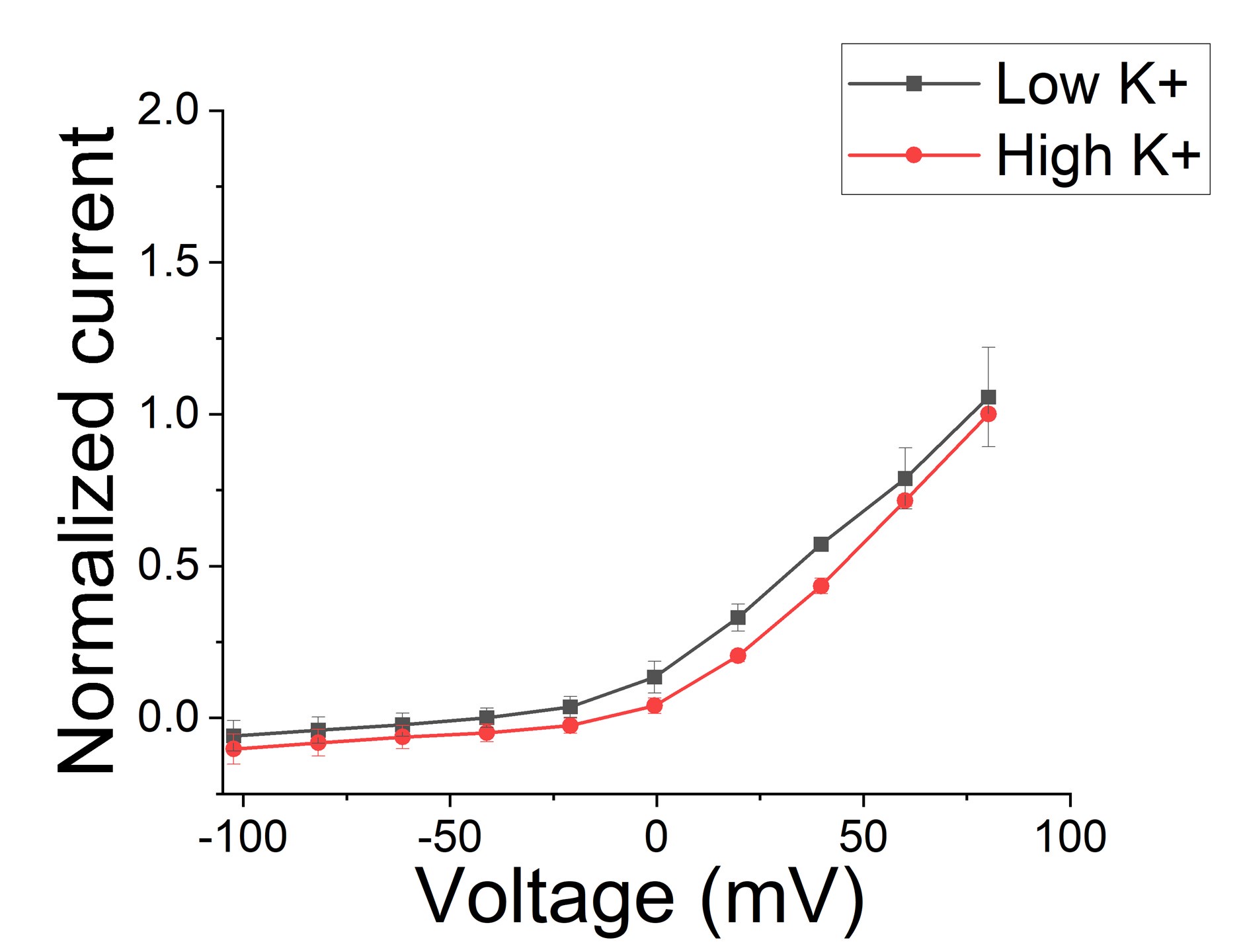
Note also that, in the previous version of the manuscript, we did not propose that the position of S4 is what determines the state of the selectivity filter. We only reported that the CryoEM structure with S4 resting shows a distorted selectivity filter. It seems like our text confused the reviewer to think that we proposed that S4 determines the state of the selectivity filter, when we did not propose this earlier. We previously did not want to speculate too much about this, but we have now included a section in the Discussion to make our view clear in light of the confusion of the reviewers.
It is clear from our data that the majority of sweeps are empty (which we assume is with S4 up), suggesting that the selectivity filter can be (and is in the majority of sweeps) in the non-conducting state even with S4 up. We think that the selectivity filter switches between a non-conductive and a conductive conformation both with S4 down and with S4 up. The cryoEM structure in low K+ and S4 down just happened to catch the non-conductive state of the selectivity filter. We have now added a section in the Discussion to clarify all this and explain how we think it works.
However, S4 in the active conformation seems to stabilize the conductive conformation of the selectivity filter, because during long pulses the channel seems to stay open once opened (See Suppl Fig S2). So, one possibility is that the selectivity filter goes more readily into the non-conductive state when S4 is down (and maybe, or not, low K+ plays a role) and then when S4 moves up the selectivity filter sometimes recovers into the conductive state and stays there. We now have included a section in the Discussion to present our view. Since this whole discussion was initiated and pushed by the reviewer, we hope that the reviewers will not demand more data to support these ideas. We think that this addition makes sense since other readers might have the same questions and ideas as the reviewer, and we would like to prevent any confusion about this topic.
Figure 1
It remains unclear in the manuscript itself what "control" refers to. Are control patched the same patches that later receive LG?
Yes, the control means the same patch before LG. We now indicate that in legends and text throughout.
Supplementary Figure S1
Unclear if any changes occur after addition of LG in left panel and if the LG data on right is paired in any way to data on left.
Yes, in all cases the left and right panel in all figures are from the same patch. We now indicate that in legends and text throughout.
The letter p is used both to represent open probability open probability from the all-point amplitude histogram and as a p-value statistical probability indicator sometime lower case, sometimes upper case. This was confusing.
We have now exclusively use lower case p for statistical probability and Po for open probability.
"This indicates that mutations of residues in the more intracellular region of the selectivity filter do not affect the Gmax increases and that the interactions that stabilize the channel involve only residues located near the external region part of the selectivity filter. "
Seems too strongly worded, it remains possible that mutations of other residues in the more intracellular region of the selectivity filter could affect the Gmax increases.
We have changed the text to: "Mutations of residues in the more intracellular region of the selectivity filter do not affect the Gmax increases, as if the interactions that stabilize the channel involve residues located near the external region part of the selectivity filter. "
Supplementary Figure S7
Please report Boltzmann fit parameters. What are "normalized" uA?
We removed the uA, which was mistakenly inserted. The lines in the graphs are just lines connecting the dots and not Boltzmann fits, since we don’t have saturating curves in all panels to make unique fits.
"We have previously shown that the effects of PUFAs on IKs channels involve the binding of PUFAs to two independent sites." Was binding to the sites actually shown? Suggest changing to: "We have previously proposed models in which the effects of PUFAs..."
We have now changed this as the Reviewer suggested: " We have previously proposed models in which the effects of PUFAs on IKs channels involve the binding of PUFAs to two independent sites."
Statistics used not always clear. Methods refer to multiple statistical tests but it is not clear which is used when.
We use two different tests and it is now explained in figure legends when either was used.
n values confusing. Sometimes # of sweeps used as n. Sometimes # patches used as n. In one instance "The average current during the single channel sweeps was increased by 2.3 {plus minus} 0.33 times (n = 4 patches, p =0.0006)" ...this sems a low p value for this n=4 sample?
We have now more clearly indicated what n stands for in each case. There was an extra 0 in the p value, so now it is p = 0.006. Thanks for catching that error.
Reviewer #2 (Recommendations For The Authors):
I still have some comments for the revised manuscript.
(1) (From the previous minor point #6) Since D317E and T309S did not show statistical significance in Figure 5A, the sentences such as "This data shows that Y315 and D317 are necessary for the ability of Lin-Glycine to increase Gmax" or "the effect of Lin-Glycine on Gmax of the KCNQ1/KCNE1 mutant was noticeably reduced compared to the WT channel showing the this residue contributes to the Gmax effect (Figure 5A)." may need to be toned down. Alternatively, I suggest the authors refer to Supplementary Figure S7 to confirm that Y315 and D317 are critical for increasing Gmax.
We have redone the analysis and statistical evaluation in Fig 5. We no use the more appropriate value of the fitted Gmax (which use the whole dose response curve instead of only the 20 mM value) in the statistical evaluation and now Y315F and D317E are statistically different from wt.
(2) Supplementary Fig. S1. All control diary plots include the green arrows to indicate the timing of lin-glycine (LG) application. It is a bit confusing why they are included. Is it to show that LG application did not have an immediate effect? Are the LG-free plots not available?
Not sure what the Reviewer is asking about? In the previous review round the Reviewers asked specifically for this. The arrow shows when LG was applied and the plot on the right shows the effect of LG from the same patch.
(3) The legend to Supplementary Figure S4, "The side chain of residues ... are highlighted as sticks and colored based on the atomic displacement values, from white to blue to red on a scale of 0 to 9 Å." They look mostly blue (or light blue). Which one is colored white? It might be better to use a different color code. It would also be nice to link the color code to the colors of Supplementary Figure S5, which currently uses a single color.
We have removed “from white to blue to red on a scale of 0 to 9 Å” and instead now include a color scale directly in Fig S4 to show how much each atom moved based on the color.
We feel it is not necessary to include color in Fig S5 since the scale of how much each atom moves is shown on the y axis.
(4) Add unit (pA) to the y-axis of Supplementary Figure S2.
pA has been added.
Reviewer #3 (Recommendations For The Authors):
Some issues on how data support conclusions are identified. Further justifications are suggested.
186: “The decrease in first latency is most likely due to an effect of Lin-Glycine on Site I in the VSD and related to the shift in voltage dependence caused by Lin-Glycine." The results in Fig S1B do not seem to support this statement since the mutation Y315F in the pore helix seemed to have eliminated the effect of Lin-Glycine in reducing first latency. The authors may want to show that a mutation that eliminating Site I would eliminate the effect of Lin-Glycine on first latency. On the other hand, it will be also interesting to examine if another pore mutation, such as P320L (Fig 5) also reduce the effect of Lin-Glycine on first latency.
These experiments are very hard and laborious, and we feel these are outside the scope of this paper which focuses on Site II and the mechanism of increasing Gmax. Further studies of the voltage shift and latency will have to be for a future study.
The mutation D317E did not affect the effect of Lin-Glycine on Gmax significantly (Fig 5A, and Fig S7F comparing with Fig S7A), but the authors conclude that D317 is important for Lin-Glycine association. This conclusion needs a better justification.
We have redone the analysis and statistical evaluation in Fig 5. We no use the more appropriate value of the fitted Gmax (which use the whole dose response curve instead of only the 20 mM value) in the statistical evaluation and now D317E is statistically different from wt
Author response:
The following is the authors’ response to the previous reviews.
As you can see from the assessment (which is unchanged from before) and the reviews included below, the reviewers felt that the revisions did not yet address all of the major concerns. There was agreement that the strength of evidence would be upgraded to "solid" by addressing, at minimum, the following:
(1) Which of the results are significant for individual monkeys; and
(2) How trials from different target contrasts were analyzed
In this revision, we have addressed the two primary editorial recommendations:
(1) We apologize if this information was not clear in the previous version. We have updated Table 1 to highlight clearly the significant results for individual monkeys. Six of our key results – pupil diameter (Fig 2B), microsaccades (Fig 2D), decoding performance for narrow-spiking units (Fig 3A), decoding performance for broad-spiking units (Fig 3B), target-evoked firing rate for all units (Fig 3E) and target-evoked firing rate for broad-spiking units (Fig 3F) – are significant for individual animals and therefore gives us high confidence regarding our results. Please also note that we present all results for individual animals in the Supplementary figures accompanying each main figure.
(2) We have updated the manuscript and methods to explain how trials of each contrast were included in each analysis, and how contrast normalization was performed for the analysis in Figure 3. In addition, we discuss this point in the Discussion section, which we quote below:
“Non-target stimulus contrasts were slightly different between hits and misses (mean: 33.1% in hits, 34.0% in misses, permutation test, 𝑝 = 0.02), but the contrast of the target was higher in hits compared to misses (mean: 38.7% in hits, 27.7% in misses, permutation test, 𝑝 = 1.6 𝑒 − 31). To control for potential effects of stimulus contrast, firing rates were first normalized by contrast before performing the analyses reported in Figure 3. For all other results, we considered only non-target stimuli, which had very minor differences in contrast (<1%) across hits and misses. In fact, this minor difference was in the opposite direction of our results with mean contrast being slightly higher for misses. While we cannot completely rule out any other effects of stimulus contrast, the normalization in Figure 3 and minor differences for non-target stimuli should minimize them.”
Reviewer #1 (Public Review):
Summary:
In this study, Nandy and colleagues examine neural, physiological and behavioral correlates of perceptual variability in monkeys performing a visual change detection task. They used a laminar probe to record from area V4 while two macaque monkeys detected a small change in stimulus orientation that occurred at a random time in one of two locations, focusing their analysis on stimulus conditions where the animal was equally likely to detect (hit) or not-detect (miss) a briefly presented orientation change (target). They discovered two behavioral and physiological measures that are significantly different between hit and miss trials - pupil size tends to be slightly larger on hits vs. misses, and monkeys are more likely to miss the target on trials in which they made a microsaccade shortly before target onset. They also examined multiple measures of neural activity across the cortical layers and found some measures that are significantly different between hits and misses.
Strengths:
Overall the study is well executed and the analyses are appropriate (though several issues still need to be addressed as discussed in Specific Comments).
Thank you.
Weaknesses:
My main concern with this study is that, with the exception of the pre-target microsaccades, the correlates of perceptual variability (differences between hits and misses) appear to be weak, potentially unreliable and disconnected. The GLM analysis of predictive power of trial outcome based on the behavioral and neural measures is only discussed at the end of the paper. This analysis shows that some of the measures have no significant predictive power, while others cannot be examined using the GLM analysis because these measures cannot be estimated in single trials. Given these weak and disconnected effects, my overall sense is that the current results provide limited advance to our understanding of the neural basis of perceptual variability.
Please see our response above to item #1 of the editorial recommendation. Six of our key results are individually significant in both animals giving us high confidence about the reliability and strength of our results.
Regarding the reviewer’s comment about the GLM, we note (also stated in the manuscript) that among the measures that we could estimate reliably on a single trial basis, two of these – pre-target microsaccades and input-layer firing rates – were reliable signatures of stimulus perception at threshold. This analysis does not imply that the other measures – Fano Factor, PPC, inter-laminar population correlations, SSC (which are all standard tools in modern systems neuroscience, and which cannot be estimated on a single-trial basis) – are irrelevant. Our intent in including the GLM analyses was to complement the results reported from these across-trial measures (Figs 4-7) with the predictive power of single-trial measures.
While no study is entirely complete in itself, we have attempted to synthesize our results into a conceptual model as depicted in Fig 8.
Reviewer #2 (Public Review):
Strengths:
The experiments were well-designed and executed with meticulous control. The analyses of both behavioural and electrophysiological data align with the standards in the field.
Thank you.
Weaknesses:
Many of the findings appear to be subtle differences and incremental compared to previous literature, including the authors' own work. While incremental findings are not necessarily a problem, the manuscript lacks clear statements about the extent to which the dataset, analysis, and findings overlap with the authors' prior research. For example, one of the main findings, which suggests that V4 neurons exhibit larger visual responses in hit trials (as shown in Fig. 3), appears to have been previously reported in their 2017 paper.
We respectfully disagree with the assessment that the findings reported here are incremental over the results reported in our prior study (Nandy et al,. 2017). In the previous study, we compared the laminar profile of neural modulation due to the deployment of attention i.e. the main comparison points were the attend-in and the attend-away conditions while controlling for visual stimulation. In this study, we go one step further and home in on the attend-in condition and investigate the differences in the laminar profile of neural activity (and two additional physiological measures: pupil and microsaccades) when the animal either correctly reports or fails to report a stimulus with equal probability. We thus control for both the visual stimulation and the cued attention state of the animal. While there are parallels to our previous results (as the reviewer correctly noted), the results reported here cannot be trivially predicted from our previous results. Please also note that we discuss our new results in the context of prior results, from both our group and others, in the manuscript (lines 310-332).
Furthermore, the manuscript does not explore potentially interesting aspects of the dataset. For instance, the authors could have investigated instances where monkeys made 'false' reports, such as executing saccades towards visual stimuli when no orientation change occurred, which allows for a broader analysis that considers the perceptual component of neural activity over pure sensory responses. Overall, lacking broad interest with the current form.
We appreciate the reviewer’s feedback on analyzing false alarm trials. Our focus for this study was to investigate the behavioral and neural correlates accompanying a correct or incorrect perception of a target stimulus presented at perceptual threshold. False alarm trials, by definition, do not include a target presentation. Moreover, false alarm rates rapidly decline with duration into a trial, with high rates during the first non-target presentation and rates close to zero by the time of the eighth presentation (see figure). Investigating false alarms will thus involve a completely different form of analysis than we have undertaken here. We therefore feel that while analyzing false alarm trials will be an interesting avenue to pursue in the future, it is outside the scope of the present study.
Author response image 1.
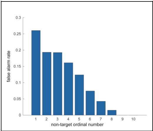
Author response:
The following is the authors’ response to the current reviews.
eLife assessment
This useful manuscript challenges the utility of current paradigms for estimating brain-age with magnetic resonance imaging measures, but presents inadequate evidence to support the suggestion that an alternative approach focused on predicting cognition is more useful. The paper would benefit from a clearer explication of the methods and a more critical evaluation of the conceptual basis of the different models. This work will be of interest to researchers working on brain-age and related models.
Thank you so much for providing high-quality reviews on our manuscript. We revised the manuscript to address all of the reviewers’ comments and provided full responses to each of the comments below. Importantly, in this revision, we clarified that we did not intend to use Brain Cognition as an alternative approach as mentioned by the editor. This is because, by design, the variation in fluid cognition explained by Brain Cognition should be higher or equal to that explained by Brain Age. Here we made this point more explicit and further stated that the relationship between Brain Cognition and fluid cognition indicates the upper limit of Brain Age’s capability in capturing fluid cognition. By examining what was captured by Brain Cognition, over and above Brain Age and chronological age via the unique effects of Brain Cognition, we were able to quantify the amount of co-variation between brain MRI and fluid cognition that was missed by Brain Age. And such quantification is the third aim of this study.
Reviewer #1 (Public Review):
In this paper, the authors evaluate the utility of brain age derived metrics for predicting cognitive decline by performing a 'commonality' analysis in a downstream regression that enables the different contribution of different predictors to be assessed. The main conclusion is that brain age derived metrics do not explain much additional variation in cognition over and above what is already explained by age. The authors propose to use a regression model trained to predict cognition ('brain cognition') as an alternative suited to applications of cognitive decline. While this is less accurate overall than brain age, it explains more unique variance in the downstream regression.
Importantly, in this revision, we clarified that we did not intend to use Brain Cognition as an alternative approach. This is because, by design, the variation in fluid cognition explained by Brain Cognition should be higher or equal to that explained by Brain Age. Here we made this point more explicit and further stated that the relationship between Brain Cognition and fluid cognition indicates the upper limit of Brain Age’s capability in capturing fluid cognition. By examining what was captured by Brain Cognition, over and above Brain Age and chronological age via the unique effects of Brain Cognition, we were able to quantify the amount of co-variation between brain MRI and fluid cognition that was missed by Brain Age.
REVISED VERSION: while the authors have partially addressed my concerns, I do not feel they have addressed them all. I do not feel they have addressed the weight instability and concerns about the stacked regression models satisfactorily.
Please see our responses to #3 below
I also must say that I agree with Reviewer 3 about the limitations of the brain age and brain cognition methods conceptually. In particular that the regression model used to predict fluid cognition will by construction explain more variance in cognition than a brain age model that is trained to predict age. This suffers from the same problem the authors raise with brain age and would indeed disappear if the authors had a separate measure of cognition against which to validate and were then to regress this out as they do for age correction. I am aware that these conceptual problems are more widespread than this paper alone (in fact throughout the brain age literature), so I do not believe the authors should be penalised for that. However, I do think they can make these concerns more explicit and further tone down the comments they make about the utility of brain cognition. I have indicated the main considerations about these points in the recommendations section below.
Thank you so much for raising this point. We now have the following statement in the introduction and discussion to address this concern (see below).
Briefly, we made it explicit that, by design, the variation in fluid cognition explained by Brain Cognition should be higher or equal to that explained by Brain Age. That is, the relationship between Brain Cognition and fluid cognition indicates the upper limit of Brain Age’s capability in capturing fluid cognition. More importantly, by examining what was captured by Brain Cognition, over and above Brain Age and chronological age via the unique effects of Brain Cognition, we were able to quantify the amount of co-variation between brain MRI and fluid cognition that was missed by Brain Age. And this is the third goal of this present study.
From Introduction:
“Third and finally, certain variation in fluid cognition is related to brain MRI, but to what extent does Brain Age not capture this variation? To estimate the variation in fluid cognition that is related to the brain MRI, we could build prediction models that directly predict fluid cognition (i.e., as opposed to chronological age) from brain MRI data. Previous studies found reasonable predictive performances of these cognition-prediction models, built from certain MRI modalities (Dubois et al., 2018; Pat, Wang, Anney, et al., 2022; Rasero et al., 2021; Sripada et al., 2020; Tetereva et al., 2022; for review, see Vieira et al., 2022). Analogous to Brain Age, we called the predicted values from these cognition-prediction models, Brain Cognition. The strength of an out-of-sample relationship between Brain Cognition and fluid cognition reflects variation in fluid cognition that is related to the brain MRI and, therefore, indicates the upper limit of Brain Age’s capability in capturing fluid cognition. This is, by design, the variation in fluid cognition explained by Brain Cognition should be higher or equal to that explained by Brain Age. Consequently, if we included Brain Cognition, Brain Age and chronological age in the same model to explain fluid cognition, we would be able to examine the unique effects of Brain Cognition that explain fluid cognition beyond Brain Age and chronological age. These unique effects of Brain Cognition, in turn, would indicate the amount of co-variation between brain MRI and fluid cognition that is missed by Brain Age.”
From Discussion:
“Third, by introducing Brain Cognition, we showed the extent to which Brain Age indices were not able to capture the variation in fluid cognition that is related to brain MRI. More specifically, using Brain Cognition allowed us to gauge the variation in fluid cognition that is related to the brain MRI, and thereby, to estimate the upper limit of what Brain Age can do. Moreover, by examining what was captured by Brain Cognition, over and above Brain Age and chronological age via the unique effects of Brain Cognition, we were able to quantify the amount of co-variation between brain MRI and fluid cognition that was missed by Brain Age.
From our results, Brain Cognition, especially from certain cognition-prediction models such as the stacked models, has relatively good predictive performance, consistent with previous studies (Dubois et al., 2018; Pat, Wang, Anney, et al., 2022; Rasero et al., 2021; Sripada et al., 2020; Tetereva et al., 2022; for review, see Vieira et al., 2022). We then examined Brain Cognition using commonality analyses (Nimon et al., 2008) in multiple regression models having a Brain Age index, chronological age and Brain Cognition as regressors to explain fluid cognition. Similar to Brain Age indices, Brain Cognition exhibited large common effects with chronological age. But more importantly, unlike Brain Age indices, Brain Cognition showed large unique effects, up to around 11%. As explained above, the unique effects of Brain Cognition indicated the amount of co-variation between brain MRI and fluid cognition that was missed by a Brain Age index and chronological age. This missing amount was relatively high, considering that Brain Age and chronological age together explained around 32% of the total variation in fluid cognition. Accordingly, if a Brain Age index was used as a biomarker along with chronological age, we would have missed an opportunity to improve the performance of the model by around one-third of the variation explained.”
This is a reasonably good paper and the use of a commonality analysis is a nice contribution to understanding variance partitioning across different covariates. I have some comments that I believe the authors ought to address, which mostly relate to clarity and interpretation
Reviewer #1 Public Review #1
First, from a conceptual point of view, the authors focus exclusively on cognition as a downstream outcome. I would suggest the authors nuance their discussion to provide broader considerations of the utility of their method and on the limits of interpretation of brain age models more generally.
Thank you for your comments on this issue.
We now discussed the broader consideration in detail:
(1) the consistency between our findings on fluid cognition and other recent works on brain disorders,
(2) the difference between studies investigating the utility of Brain Age in explaining cognitive functioning, including ours and others (e.g., Butler et al., 2021; Cole, 2020, 2020; Jirsaraie, Kaufmann, et al., 2023) and those explaining neurological/psychological disorders (e.g., Bashyam et al., 2020; Rokicki et al., 2021)
and
(3) suggested solutions we and others made to optimise the utility of Brain Age for both cognitive functioning and brain disorders.
From Discussion:
“This discrepancy between the predictive performance of age-prediction models and the utility of Brain Age indices as a biomarker is consistent with recent findings (for review, see Jirsaraie, Gorelik, et al., 2023), both in the context of cognitive functioning (Jirsaraie, Kaufmann, et al., 2023) and neurological/psychological disorders (Bashyam et al., 2020; Rokicki et al., 2021). For instance, combining different MRI modalities into the prediction models, similar to our stacked models, often leads to the highest performance of age-prediction models, but does not likely explain the highest variance across different phenotypes, including cognitive functioning and beyond (Jirsaraie, Gorelik, et al., 2023).”
“There is a notable difference between studies investigating the utility of Brain Age in explaining cognitive functioning, including ours and others (e.g., Butler et al., 2021; Cole, 2020, 2020; Jirsaraie, Kaufmann, et al., 2023) and those explaining neurological/psychological disorders (e.g., Bashyam et al., 2020; Rokicki et al., 2021). We consider the former as a normative type of study and the latter as a case-control type of study (Insel et al., 2010; Marquand et al., 2016). Those case-control Brain Age studies focusing on neurological/psychological disorders often build age-prediction models from MRI data of largely healthy participants (e.g., controls in a case-control design or large samples in a population-based design), apply the built age-prediction models to participants without vs. with neurological/psychological disorders and compare Brain Age indices between the two groups. On the one hand, this means that case-control studies treat Brain Age as a method to detect anomalies in the neurological/psychological group (Hahn et al., 2021). On the other hand, this also means that case-control studies have to ignore under-fitted models when applied prediction models built from largely healthy participants to participants with neurological/psychological disorders (i.e., Brain Age may predict chronological age well for the controls, but not for those with a disorder). On the contrary, our study and other normative studies focusing on cognitive functioning often build age-prediction models from MRI data of largely healthy participants and apply the built age-prediction models to participants who are also largely healthy. Accordingly, the age-prediction models for explaining cognitive functioning in normative studies, while not allowing us to detect group-level anomalies, do not suffer from being under-fitted. This unfortunately might limit the generalisability of our study into just the normative type of study. Future work is still needed to test the utility of brain age in the case-control case.”
“Next, researchers should not select age-prediction models based solely on age-prediction performance. Instead, researchers could select age-prediction models that explained phenotypes of interest the best. Here we selected age-prediction models based on a set of features (i.e., modalities) of brain MRI. This strategy was found effective not only for fluid cognition as we demonstrated here, but also for neurological and psychological disorders as shown elsewhere (Jirsaraie, Gorelik, et al., 2023; Rokicki et al., 2021). Rokicki and colleagues (2021), for instance, found that, while integrating across MRI modalities led to age-prediction models with the highest age-prediction performance, using only T1 structural MRI gave age-prediction models that were better at classifying Alzheimer’s disease. Similarly, using only cerebral blood flow gave age-prediction models that were better at classifying mild/subjective cognitive impairment, schizophrenia and bipolar disorder.
As opposed to selecting age-prediction models based on a set of features, researchers could also select age-prediction models based on modelling methods. For instance, Jirsaraie and colleagues (2023) compared gradient tree boosting (GTB) and deep-learning brain network (DBN) algorithms in building age-prediction models. They found GTB to have higher age-prediction performance but DBN to have better utility in explaining cognitive functioning. In this case, an algorithm with better utility (e.g., DBN) should be used for explaining a phenotype of interest. Similarly, Bashyam and colleagues (2020) built different DBN-based age-prediction models, varying in age-prediction performance. The DBN models with a higher number of epochs corresponded to higher age-prediction performance. However, DBN-based age-prediction models with a moderate (as opposed to higher or lower) number of epochs were better at classifying Alzheimer’s disease, mild cognitive impairment and schizophrenia. In this case, a model from the same algorithm with better utility (e.g., those DBN with a moderate epoch number) should be used for explaining a phenotype of interest. Accordingly, this calls for a change in research practice, as recently pointed out by Jirasarie and colleagues (2023, p7), “Despite mounting evidence, there is a persisting assumption across several studies that the most accurate brain age models will have the most potential for detecting differences in a given phenotype of interest”. Future neuroimaging research should aim to build age-prediction models that are not necessarily good at predicting age, but at capturing phenotypes of interest.”
Reviewer #1 Public Review #2
Second, from a methods perspective, there is not a sufficient explanation of the methodological procedures in the current manuscript to fully understand how the stacked regression models were constructed. I would request that the authors provide more information to enable the reader to better understand the stacked regression models used to ensure that these models are not overfit.
Thank you for allowing us an opportunity to clarify our stacked model. We made additional clarification to make this clearer (see below). We wanted to confirm that we did not use test sets to build a stacked model in both lower and higher levels of the Elastic Net models. Test sets were there just for testing the performance of the models.
From Methods: “We used nested cross-validation (CV) to build these prediction models (see Figure 7). We first split the data into five outer folds, leaving each outer fold with around 100 participants. This number of participants in each fold is to ensure the stability of the test performance across folds. In each outer-fold CV loop, one of the outer folds was treated as an outer-fold test set, and the rest was treated as an outer-fold training set. Ultimately, looping through the nested CV resulted in a) prediction models from each of the 18 sets of features as well as b) prediction models that drew information across different combinations of the 18 separate sets, known as “stacked models.” We specified eight stacked models: “All” (i.e., including all 18 sets of features), “All excluding Task FC”, “All excluding Task Contrast”, “Non-Task” (i.e., including only Rest FC and sMRI), “Resting and Task FC”, “Task Contrast and FC”, “Task Contrast” and “Task FC”. Accordingly, there were 26 prediction models in total for both Brain Age and Brain Cognition.
To create these 26 prediction models, we applied three steps for each outer-fold loop. The first step aimed at tuning prediction models for each of 18 sets of features. This step only involved the outer-fold training set and did not involve the outer-fold test set. Here, we divided the outer-fold training set into five inner folds and applied inner-fold CV to tune hyperparameters with grid search. Specifically, in each inner-fold CV, one of the inner folds was treated as an inner-fold validation set, and the rest was treated as an inner-fold training set. Within each inner-fold CV loop, we used the inner-fold training set to estimate parameters of the prediction model with a particular set of hyperparameters and applied the estimated model to the inner-fold validation set. After looping through the inner-fold CV, we, then, chose the prediction models that led to the highest performance, reflected by coefficient of determination (R2), on average across the inner-fold validation sets. This led to 18 tuned models, one for each of the 18 sets of features, for each outer fold.
The second step aimed at tuning stacked models. Same as the first step, the second step only involved the outer-fold training set and did not involve the outer-fold test set. Here, using the same outer-fold training set as the first step, we applied tuned models, created from the first step, one from each of the 18 sets of features, resulting in 18 predicted values for each participant. We, then, re-divided this outer-fold training set into new five inner folds. In each inner fold, we treated different combinations of the 18 predicted values from separate sets of features as features to predict the targets in separate “stacked” models. Same as the first step, in each inner-fold CV loop, we treated one out of five inner folds as an inner-fold validation set, and the rest as an inner-fold training set. Also as in the first step, we used the inner-fold training set to estimate parameters of the prediction model with a particular set of hyperparameters from our grid. We tuned the hyperparameters of stacked models using grid search by selecting the models with the highest R2 on average across the inner-fold validation sets. This led to eight tuned stacked models.
The third step aimed at testing the predictive performance of the 18 tuned prediction models from each of the set of features, built from the first step, and eight tuned stacked models, built from the second step. Unlike the first two steps, here we applied the already tuned models to the outer-fold test set. We started by applying the 18 tuned prediction models from each of the sets of features to each observation in the outer-fold test set, resulting in 18 predicted values. We then applied the tuned stacked models to these predicted values from separate sets of features, resulting in eight predicted values.
To demonstrate the predictive performance, we assessed the similarity between the observed values and the predicted values of each model across outer-fold test sets, using Pearson’s r, coefficient of determination (R2) and mean absolute error (MAE). Note that for R2, we used the sum of squares definition (i.e., R2 = 1 – (sum of squares residuals/total sum of squares)) per a previous recommendation (Poldrack et al., 2020). We considered the predicted values from the outer-fold test sets of models predicting age or fluid cognition, as Brain Age and Brain Cognition, respectively.”
Note some previous research, including ours (Tetereva et al., 2022), splits the observations in the outer-fold training set into layer 1 and layer 2 and applies the first and second steps to layers 1 and 2, respectively. Here we decided against this approach and used the same outer-fold training set for both first and second steps in order to avoid potential bias toward the stacked models. This is because, when the data are split into two layers, predictive models built for each separate set of features only use the data from layer 1, while the stacked models use the data from both layers 1 and 2. In practice with large enough data, these two approaches might not differ much, as we demonstrated previously (Tetereva et al., 2022).
Reviewer #1 Public Review #3
Please also provide an indication of the different regression strengths that were estimated across the different models and cross-validation splits. Also, how stable were the weights across splits?
The focus of this article is on the predictions. Still, it is informative for readers to understand how stable the feature importance (i.e., Elastic Net coefficients) is. To demonstrate the stability of feature importance, we now examined the rank stability of feature importance using Spearman’s ρ (see Figure 4). Specifically, we correlated the feature importance between two prediction models of the same features, used in two different outer-fold test sets. Given that there were five outer-fold test sets, we computed 10 Spearman’s ρ for each prediction model of the same features. We found Spearman’s ρ to be varied dramatically in both age-prediction (range=.31-.94) and fluid cognition-prediction (range=.16-.84) models. This means that some prediction models were much more stable in their feature importance than others. This is probably due to various factors such as a) the collinearity of features in the model, b) the number of features (e.g., 71,631 features in functional connectivity, which were further reduced to 75 PCAs, as compared to 19 features in subcortical volume based on the ASEG atlas), c) the penalisation of coefficients either with ‘Ridge’ or ‘Lasso’ methods, which resulted in reduction as a group of features or selection of a feature among correlated features, respectively, and d) the predictive performance of the models. Understanding the stability of feature importance is beyond the scope of the current article. As mentioned by Reviewer 1, “The predictions can be stable when the coefficients are not,” and we chose to focus on the prediction in the current article.
Reviewer #1 Public Review #4
Please provide more details about the task designs, MRI processing procedures that were employed on this sample in addition to the regression methods and bias correction methods used. For example, there are several different parameterisations of the elastic net, please provide equations to describe the method used here so that readers can easily determine how the regularisation parameters should be interpreted.
Thank you for the opportunity for us to provide more methodical details.
First, for the task design, we included the following statements:
From Methods:
“HCP-A collected fMRI data from three tasks: Face Name (Sperling et al., 2001), Conditioned Approach Response Inhibition Task (CARIT) (Somerville et al., 2018) and VISual MOTOR (VISMOTOR) (Ances et al., 2009).
First, the Face Name task (Sperling et al., 2001) taps into episodic memory. The task had three blocks. In the encoding block [Encoding], participants were asked to memorise the names of faces shown. These faces were then shown again in the recall block [Recall] when the participants were asked if they could remember the names of the previously shown faces. There was also the distractor block [Distractor] occurring between the encoding and recall blocks. Here participants were distracted by a Go/NoGo task. We computed six contrasts for this Face Name task: [Encode], [Recall], [Distractor], [Encode vs. Distractor], [Recall vs. Distractor] and [Encode vs. Recall].
Second, the CARIT task (Somerville et al., 2018) was adapted from the classic Go/NoGo task and taps into inhibitory control. Participants were asked to press a button to all [Go] but not to two [NoGo] shapes. We computed three contrasts for the CARIT task: [NoGo], [Go] and [NoGo vs. Go].
Third, the VISMOTOR task (Ances et al., 2009) was designed to test simple activation of the motor and visual cortices. Participants saw a checkerboard with a red square either on the left or right. They needed to press a corresponding key to indicate the location of the red square. We computed just one contrast for the VISMOTOR task: [Vismotor], which indicates the presence of the checkerboard vs. baseline.”
Second, for MRI processing procedures, we included the following statements.
From Methods: “HCP-A provides details of parameters for brain MRI elsewhere (Bookheimer et al., 2019; Harms et al., 2018). Here we used MRI data that were pre-processed by the HCP-A with recommended methods, including the MSMALL alignment (Glasser et al., 2016; Robinson et al., 2018) and ICA-FIX (Glasser et al., 2016) for functional MRI. We used multiple brain MRI modalities, covering task functional MRI (task fMRI), resting-state functional MRI (rsfMRI) and structural MRI (sMRI), and organised them into 19 sets of features.”
“ Sets of Features 1-10: Task fMRI contrast (Task Contrast) Task contrasts reflect fMRI activation relevant to events in each task. Bookheimer and colleagues (2019) provided detailed information about the fMRI in HCP-A. Here we focused on the pre-processed task fMRI Connectivity Informatics Technology Initiative (CIFTI) files with a suffix, “_PA_Atlas_MSMAll_hp0_clean.dtseries.nii.” These CIFTI files encompassed both the cortical mesh surface and subcortical volume (Glasser et al., 2013). Collected using the posterior-to-anterior (PA) phase, these files were aligned using MSMALL (Glasser et al., 2016; Robinson et al., 2018), linear detrended (see https://groups.google.com/a/humanconnectome.org/g/hcp-users/c/ZLJc092h980/m/GiihzQAUAwAJ) and cleaned from potential artifacts using ICA-FIX (Glasser et al., 2016).
To extract Task Contrasts, we regressed the fMRI time series on the convolved task events using a double-gamma canonical hemodynamic response function via FMRIB Software Library (FSL)’s FMRI Expert Analysis Tool (FEAT) (Woolrich et al., 2001). We kept FSL’s default high pass cutoff at 200s (i.e., .005 Hz). We then parcellated the contrast ‘cope’ files, using the Glasser atlas (Gordon et al., 2016) for cortical surface regions and the Freesurfer’s automatic segmentation (aseg) (Fischl et al., 2002) for subcortical regions. This resulted in 379 regions, whose number was, in turn, the number of features for each Task Contrast set of features. “
“ Sets of Features 11-13: Task fMRI functional connectivity (Task FC) Task FC reflects functional connectivity (FC ) among the brain regions during each task, which is considered an important source of individual differences (Elliott et al., 2019; Fair et al., 2007; Gratton et al., 2018). We used the same CIFTI file “_PA_Atlas_MSMAll_hp0_clean.dtseries.nii.” as the task contrasts. Unlike Task Contrasts, here we treated the double-gamma, convolved task events as regressors of no interest and focused on the residuals of the regression from each task (Fair et al., 2007). We computed these regressors on FSL, and regressed them in nilearn (Abraham et al., 2014). Following previous work on task FC (Elliott et al., 2019), we applied a highpass at .008 Hz. For parcellation, we used the same atlases as Task Contrast (Fischl et al., 2002; Glasser et al., 2016). We computed Pearson’s correlations of each pair of 379 regions, resulting in a table of 71,631 non-overlapping FC indices for each task. We then applied r-to-z transformation and principal component analysis (PCA) of 75 components (Rasero et al., 2021; Sripada et al., 2019, 2020). Note to avoid data leakage, we conducted the PCA on each training set and applied its definition to the corresponding test set. Accordingly, there were three sets of 75 features for Task FC, one for each task.
Set of Features 14: Resting-state functional MRI functional connectivity (Rest FC) Similar to Task FC, Rest FC reflects functional connectivity (FC ) among the brain regions, except that Rest FC occurred during the resting (as opposed to task-performing) period. HCP-A collected Rest FC from four 6.42-min (488 frames) runs across two days, leading to 26-min long data (Harms et al., 2018). On each day, the study scanned two runs of Rest FC, starting with anterior-to-posterior (AP) and then with posterior-to-anterior (PA) phase encoding polarity. We used the “rfMRI_REST_Atlas_MSMAll_hp0_clean.dscalar.nii” file that was pre-processed and concatenated across the four runs. We applied the same computations (i.e., highpass filter, parcellation, Pearson’s correlations, r-to-z transformation and PCA) with the Task FC.
Sets of Features 15-18: Structural MRI (sMRI)
sMRI reflects individual differences in brain anatomy. The HCP-A used an established pre-processing pipeline for sMRI (Glasser et al., 2013). We focused on four sets of features: cortical thickness, cortical surface area, subcortical volume and total brain volume. For cortical thickness and cortical surface area, we used Destrieux’s atlas (Destrieux et al., 2010; Fischl, 2012) from FreeSurfer’s “aparc.stats” file, resulting in 148 regions for each set of features. For subcortical volume, we used the aseg atlas (Fischl et al., 2002) from FreeSurfer’s “aseg.stats” file, resulting in 19 regions. For total brain volume, we had five FreeSurfer-based features: “FS_IntraCranial_Vol” or estimated intra-cranial volume, “FS_TotCort_GM_Vol” or total cortical grey matter volume, “FS_Tot_WM_Vol” or total cortical white matter volume, “FS_SubCort_GM_Vol” or total subcortical grey matter volume and “FS_BrainSegVol_eTIV_Ratio” or ratio of brain segmentation volume to estimated total intracranial volume.”
Third, for regression methods and bias correction methods used, we included the following statements:
From Methods:
“For the machine learning algorithm, we used Elastic Net (Zou & Hastie, 2005). Elastic Net is a general form of penalised regressions (including Lasso and Ridge regression), allowing us to simultaneously draw information across different brain indices to predict one target variable. Penalised regressions are commonly used for building age-prediction models (Jirsaraie, Gorelik, et al., 2023). Previously we showed that the performance of Elastic Net in predicting cognitive abilities is on par, if not better than, many non-linear and more-complicated algorithms (Pat, Wang, Bartonicek, et al., 2022; Tetereva et al., 2022). Moreover, Elastic Net coefficients are readily explainable, allowing us the ability to explain how our age-prediction and cognition-prediction models made the prediction from each brain feature (Molnar, 2019; Pat, Wang, Bartonicek, et al., 2022) (see below).
Elastic Net simultaneously minimises the weighted sum of the features’ coefficients. The degree of penalty to the sum of the feature’s coefficients is determined by a shrinkage hyperparameter ‘α’: the greater the α, the more the coefficients shrink, and the more regularised the model becomes. Elastic Net also includes another hyperparameter, ‘l1 ratio’, which determines the degree to which the sum of either the squared (known as ‘Ridge’; l1 ratio=0) or absolute (known as ‘Lasso’; l1 ratio=1) coefficients is penalised (Zou & Hastie, 2005). The objective function of Elastic Net as implemented by sklearn (Pedregosa et al., 2011) is defined as:

where X is the features, y is the target, and β is the coefficient. In our grid search, we tuned two Elastic Net hyperparameters: α using 70 numbers in log space, ranging from .1 and 100, and l_1-ratio using 25 numbers in linear space, ranging from 0 and 1.
To understand how Elastic Net made a prediction based on different brain features, we examined the coefficients of the tuned model. Elastic Net coefficients can be considered as feature importance, such that more positive Elastic Net coefficients lead to more positive predicted values and, similarly, more negative Elastic Net coefficients lead to more negative predicted values (Molnar, 2019; Pat, Wang, Bartonicek, et al., 2022). While the magnitude of Elastic Net coefficients is regularised (thus making it difficult for us to interpret the magnitude itself directly), we could still indicate that a brain feature with a higher magnitude weights relatively stronger in making a prediction. Another benefit of Elastic Net as a penalised regression is that the coefficients are less susceptible to collinearity among features as they have already been regularised (Dormann et al., 2013; Pat, Wang, Bartonicek, et al., 2022).
Given that we used five-fold nested cross validation, different outer folds may have different degrees of ‘α’ and ‘l1 ratio’, making the final coefficients from different folds to be different. For instance, for certain sets of features, penalisation may not play a big part (i.e., higher or lower ‘α’ leads to similar predictive performance), resulting in different ‘α’ for different folds. To remedy this in the visualisation of Elastic Net feature importance, we refitted the Elastic Net model to the full dataset without splitting them into five folds and visualised the coefficients on brain images using Brainspace (Vos De Wael et al., 2020) and Nilern (Abraham et al., 2014) packages. Note, unlike other sets of features, Task FC and Rest FC were modelled after data reduction via PCA. Thus, for Task FC and Rest FC, we, first, multiplied the absolute PCA scores (extracted from the ‘components_’ attribute of ‘sklearn.decomposition.PCA’) with Elastic Net coefficients and, then, summed the multiplied values across the 75 components, leaving 71,631 ROI-pair indices. “
References
Abraham, A., Pedregosa, F., Eickenberg, M., Gervais, P., Mueller, A., Kossaifi, J., Gramfort, A., Thirion, B., & Varoquaux, G. (2014). Machine learning for neuroimaging with scikit-learn. Frontiers in Neuroinformatics, 8, 14. https://doi.org/10.3389/fninf.2014.00014
Ances, B. M., Liang, C. L., Leontiev, O., Perthen, J. E., Fleisher, A. S., Lansing, A. E., & Buxton, R. B. (2009). Effects of aging on cerebral blood flow, oxygen metabolism, and blood oxygenation level dependent responses to visual stimulation. Human Brain Mapping, 30(4), 1120–1132. https://doi.org/10.1002/hbm.20574
Bashyam, V. M., Erus, G., Doshi, J., Habes, M., Nasrallah, I. M., Truelove-Hill, M., Srinivasan, D., Mamourian, L., Pomponio, R., Fan, Y., Launer, L. J., Masters, C. L., Maruff, P., Zhuo, C., Völzke, H., Johnson, S. C., Fripp, J., Koutsouleris, N., Satterthwaite, T. D., … on behalf of the ISTAGING Consortium, the P. A. disease C., ADNI, and CARDIA studies. (2020). MRI signatures of brain age and disease over the lifespan based on a deep brain network and 14 468 individuals worldwide. Brain, 143(7), 2312–2324. https://doi.org/10.1093/brain/awaa160
Bookheimer, S. Y., Salat, D. H., Terpstra, M., Ances, B. M., Barch, D. M., Buckner, R. L., Burgess, G. C., Curtiss, S. W., Diaz-Santos, M., Elam, J. S., Fischl, B., Greve, D. N., Hagy, H. A., Harms, M. P., Hatch, O. M., Hedden, T., Hodge, C., Japardi, K. C., Kuhn, T. P., … Yacoub, E. (2019). The Lifespan Human Connectome Project in Aging: An overview. NeuroImage, 185, 335–348. https://doi.org/10.1016/j.neuroimage.2018.10.009
Butler, E. R., Chen, A., Ramadan, R., Le, T. T., Ruparel, K., Moore, T. M., Satterthwaite, T. D., Zhang, F., Shou, H., Gur, R. C., Nichols, T. E., & Shinohara, R. T. (2021). Pitfalls in brain age analyses. Human Brain Mapping, 42(13), 4092–4101. https://doi.org/10.1002/hbm.25533
Cole, J. H. (2020). Multimodality neuroimaging brain-age in UK biobank: Relationship to biomedical, lifestyle, and cognitive factors. Neurobiology of Aging, 92, 34–42. https://doi.org/10.1016/j.neurobiolaging.2020.03.014
Destrieux, C., Fischl, B., Dale, A., & Halgren, E. (2010). Automatic parcellation of human cortical gyri and sulci using standard anatomical nomenclature. NeuroImage, 53(1), 1–15. https://doi.org/10.1016/j.neuroimage.2010.06.010
Dormann, C. F., Elith, J., Bacher, S., Buchmann, C., Carl, G., Carré, G., Marquéz, J. R. G., Gruber, B., Lafourcade, B., Leitão, P. J., Münkemüller, T., McClean, C., Osborne, P. E., Reineking, B., Schröder, B., Skidmore, A. K., Zurell, D., & Lautenbach, S. (2013). Collinearity: A review of methods to deal with it and a simulation study evaluating their performance. Ecography, 36(1), 27–46. https://doi.org/10.1111/j.1600-0587.2012.07348.x
Dubois, J., Galdi, P., Paul, L. K., & Adolphs, R. (2018). A distributed brain network predicts general intelligence from resting-state human neuroimaging data. Philosophical Transactions of the Royal Society B: Biological Sciences, 373(1756), 20170284. https://doi.org/10.1098/rstb.2017.0284
Elliott, M. L., Knodt, A. R., Cooke, M., Kim, M. J., Melzer, T. R., Keenan, R., Ireland, D., Ramrakha, S., Poulton, R., Caspi, A., Moffitt, T. E., & Hariri, A. R. (2019). General functional connectivity: Shared features of resting-state and task fMRI drive reliable and heritable individual differences in functional brain networks. NeuroImage, 189, 516–532. https://doi.org/10.1016/j.neuroimage.2019.01.068
Fair, D. A., Schlaggar, B. L., Cohen, A. L., Miezin, F. M., Dosenbach, N. U. F., Wenger, K. K., Fox, M. D., Snyder, A. Z., Raichle, M. E., & Petersen, S. E. (2007). A method for using blocked and event-related fMRI data to study “resting state” functional connectivity. NeuroImage, 35(1), 396–405. https://doi.org/10.1016/j.neuroimage.2006.11.051
Fischl, B. (2012). FreeSurfer. NeuroImage, 62(2), 774–781. https://doi.org/10.1016/j.neuroimage.2012.01.021
Fischl, B., Salat, D. H., Busa, E., Albert, M., Dieterich, M., Haselgrove, C., van der Kouwe, A., Killiany, R., Kennedy, D., Klaveness, S., Montillo, A., Makris, N., Rosen, B., & Dale, A. M. (2002). Whole Brain Segmentation. Neuron, 33(3), 341–355. https://doi.org/10.1016/S0896-6273(02)00569-X
Glasser, M. F., Smith, S. M., Marcus, D. S., Andersson, J. L. R., Auerbach, E. J., Behrens, T. E. J., Coalson, T. S., Harms, M. P., Jenkinson, M., Moeller, S., Robinson, E. C., Sotiropoulos, S. N., Xu, J., Yacoub, E., Ugurbil, K., & Van Essen, D. C. (2016). The Human Connectome Project’s neuroimaging approach. Nature Neuroscience, 19(9), 1175–1187. https://doi.org/10.1038/nn.4361
Glasser, M. F., Sotiropoulos, S. N., Wilson, J. A., Coalson, T. S., Fischl, B., Andersson, J. L., Xu, J., Jbabdi, S., Webster, M., Polimeni, J. R., Van Essen, D. C., & Jenkinson, M. (2013). The minimal preprocessing pipelines for the Human Connectome Project. NeuroImage, 80, 105–124. https://doi.org/10.1016/j.neuroimage.2013.04.127
Gordon, E. M., Laumann, T. O., Adeyemo, B., Huckins, J. F., Kelley, W. M., & Petersen, S. E. (2016). Generation and Evaluation of a Cortical Area Parcellation from Resting-State Correlations. Cerebral Cortex, 26(1), 288–303. https://doi.org/10.1093/cercor/bhu239
Gratton, C., Laumann, T. O., Nielsen, A. N., Greene, D. J., Gordon, E. M., Gilmore, A. W., Nelson, S. M., Coalson, R. S., Snyder, A. Z., Schlaggar, B. L., Dosenbach, N. U. F., & Petersen, S. E. (2018). Functional Brain Networks Are Dominated by Stable Group and Individual Factors, Not Cognitive or Daily Variation. Neuron, 98(2), 439-452.e5. https://doi.org/10.1016/j.neuron.2018.03.035
Hahn, T., Fisch, L., Ernsting, J., Winter, N. R., Leenings, R., Sarink, K., Emden, D., Kircher, T., Berger, K., & Dannlowski, U. (2021). From ‘loose fitting’ to high-performance, uncertainty-aware brain-age modelling. Brain, 144(3), e31–e31. https://doi.org/10.1093/brain/awaa454
Harms, M. P., Somerville, L. H., Ances, B. M., Andersson, J., Barch, D. M., Bastiani, M., Bookheimer, S. Y., Brown, T. B., Buckner, R. L., Burgess, G. C., Coalson, T. S., Chappell, M. A., Dapretto, M., Douaud, G., Fischl, B., Glasser, M. F., Greve, D. N., Hodge, C., Jamison, K. W., … Yacoub, E. (2018). Extending the Human Connectome Project across ages: Imaging protocols for the Lifespan Development and Aging projects. NeuroImage, 183, 972–984. https://doi.org/10.1016/j.neuroimage.2018.09.060
Insel, T., Cuthbert, B., Garvey, M., Heinssen, R., Pine, D. S., Quinn, K., Sanislow, C., & Wang, P. (2010). Research Domain Criteria (RDoC): Toward a New Classification Framework for Research on Mental Disorders. American Journal of Psychiatry, 167(7), 748–751. https://doi.org/10.1176/appi.ajp.2010.09091379
Jirsaraie, R. J., Gorelik, A. J., Gatavins, M. M., Engemann, D. A., Bogdan, R., Barch, D. M., & Sotiras, A. (2023). A systematic review of multimodal brain age studies: Uncovering a divergence between model accuracy and utility. Patterns, 4(4), 100712. https://doi.org/10.1016/j.patter.2023.100712
Jirsaraie, R. J., Kaufmann, T., Bashyam, V., Erus, G., Luby, J. L., Westlye, L. T., Davatzikos, C., Barch, D. M., & Sotiras, A. (2023). Benchmarking the generalizability of brain age models: Challenges posed by scanner variance and prediction bias. Human Brain Mapping, 44(3), 1118–1128. https://doi.org/10.1002/hbm.26144
Marquand, A. F., Rezek, I., Buitelaar, J., & Beckmann, C. F. (2016). Understanding Heterogeneity in Clinical Cohorts Using Normative Models: Beyond Case-Control Studies. Biological Psychiatry, 80(7), 552–561. https://doi.org/10.1016/j.biopsych.2015.12.023
Molnar, C. (2019). Interpretable Machine Learning. A Guide for Making Black Box Models Explainable. https://christophm.github.io/interpretable-ml-book/
Nimon, K., Lewis, M., Kane, R., & Haynes, R. M. (2008). An R package to compute commonality coefficients in the multiple regression case: An introduction to the package and a practical example. Behavior Research Methods, 40(2), 457–466. https://doi.org/10.3758/BRM.40.2.457
Pat, N., Wang, Y., Anney, R., Riglin, L., Thapar, A., & Stringaris, A. (2022). Longitudinally stable, brain‐based predictive models mediate the relationships between childhood cognition and socio‐demographic, psychological and genetic factors. Human Brain Mapping, hbm.26027. https://doi.org/10.1002/hbm.26027
Pat, N., Wang, Y., Bartonicek, A., Candia, J., & Stringaris, A. (2022). Explainable machine learning approach to predict and explain the relationship between task-based fMRI and individual differences in cognition. Cerebral Cortex, bhac235. https://doi.org/10.1093/cercor/bhac235
Pedregosa, F., Varoquaux, G., Gramfort, A., Michel, V., Thirion, B., Grisel, O., Blondel, M., Prettenhofer, P., Weiss, R., Dubourg, V., Vanderplas, J., Passos, A., Cournapeau, D., Brucher, M., Perrot, M., & Duchesnay, É. (2011). Scikit-learn: Machine Learning in Python. Journal of Machine Learning Research, 12(85), 2825–2830.
Poldrack, R. A., Huckins, G., & Varoquaux, G. (2020). Establishment of Best Practices for Evidence for Prediction: A Review. JAMA Psychiatry, 77(5), 534–540. https://doi.org/10.1001/jamapsychiatry.2019.3671
Rasero, J., Sentis, A. I., Yeh, F.-C., & Verstynen, T. (2021). Integrating across neuroimaging modalities boosts prediction accuracy of cognitive ability. PLOS Computational Biology, 17(3), e1008347. https://doi.org/10.1371/journal.pcbi.1008347
Robinson, E. C., Garcia, K., Glasser, M. F., Chen, Z., Coalson, T. S., Makropoulos, A., Bozek, J., Wright, R., Schuh, A., Webster, M., Hutter, J., Price, A., Cordero Grande, L., Hughes, E., Tusor, N., Bayly, P. V., Van Essen, D. C., Smith, S. M., Edwards, A. D., … Rueckert, D. (2018). Multimodal surface matching with higher-order smoothness constraints. NeuroImage, 167, 453–465. https://doi.org/10.1016/j.neuroimage.2017.10.037
Rokicki, J., Wolfers, T., Nordhøy, W., Tesli, N., Quintana, D. S., Alnæs, D., Richard, G., de Lange, A.-M. G., Lund, M. J., Norbom, L., Agartz, I., Melle, I., Nærland, T., Selbæk, G., Persson, K., Nordvik, J. E., Schwarz, E., Andreassen, O. A., Kaufmann, T., & Westlye, L. T. (2021). Multimodal imaging improves brain age prediction and reveals distinct abnormalities in patients with psychiatric and neurological disorders. Human Brain Mapping, 42(6), 1714–1726. https://doi.org/10.1002/hbm.25323
Somerville, L. H., Bookheimer, S. Y., Buckner, R. L., Burgess, G. C., Curtiss, S. W., Dapretto, M., Elam, J. S., Gaffrey, M. S., Harms, M. P., Hodge, C., Kandala, S., Kastman, E. K., Nichols, T. E., Schlaggar, B. L., Smith, S. M., Thomas, K. M., Yacoub, E., Van Essen, D. C., & Barch, D. M. (2018). The Lifespan Human Connectome Project in Development: A large-scale study of brain connectivity development in 5–21 year olds. NeuroImage, 183, 456–468. https://doi.org/10.1016/j.neuroimage.2018.08.050
Sperling, R. A., Bates, J. F., Cocchiarella, A. J., Schacter, D. L., Rosen, B. R., & Albert, M. S. (2001). Encoding novel face-name associations: A functional MRI study. Human Brain Mapping, 14(3), 129–139. https://doi.org/10.1002/hbm.1047
Sripada, C., Angstadt, M., Rutherford, S., Kessler, D., Kim, Y., Yee, M., & Levina, E. (2019). Basic Units of Inter-Individual Variation in Resting State Connectomes. Scientific Reports, 9(1), Article 1. https://doi.org/10.1038/s41598-018-38406-5
Sripada, C., Angstadt, M., Rutherford, S., Taxali, A., & Shedden, K. (2020). Toward a “treadmill test” for cognition: Improved prediction of general cognitive ability from the task activated brain. Human Brain Mapping, 41(12), 3186–3197. https://doi.org/10.1002/hbm.25007
Tetereva, A., Li, J., Deng, J. D., Stringaris, A., & Pat, N. (2022). Capturing brain‐cognition relationship: Integrating task‐based fMRI across tasks markedly boosts prediction and test‐retest reliability. NeuroImage, 263, 119588. https://doi.org/10.1016/j.neuroimage.2022.119588
Vieira, B. H., Pamplona, G. S. P., Fachinello, K., Silva, A. K., Foss, M. P., & Salmon, C. E. G. (2022). On the prediction of human intelligence from neuroimaging: A systematic review of methods and reporting. Intelligence, 93, 101654. https://doi.org/10.1016/j.intell.2022.101654
Vos De Wael, R., Benkarim, O., Paquola, C., Lariviere, S., Royer, J., Tavakol, S., Xu, T., Hong, S.-J., Langs, G., Valk, S., Misic, B., Milham, M., Margulies, D., Smallwood, J., & Bernhardt, B. C. (2020). BrainSpace: A toolbox for the analysis of macroscale gradients in neuroimaging and connectomics datasets. Communications Biology, 3(1), 103. https://doi.org/10.1038/s42003-020-0794-7
Woolrich, M. W., Ripley, B. D., Brady, M., & Smith, S. M. (2001). Temporal Autocorrelation in Univariate Linear Modeling of FMRI Data. NeuroImage, 14(6), 1370–1386. https://doi.org/10.1006/nimg.2001.0931
Zou, H., & Hastie, T. (2005). Regularization and variable selection via the elastic net. Journal of the Royal Statistical Society: Series B (Statistical Methodology), 67(2), 301–320. https://doi.org/10.1111/j.1467-9868.2005.00503.x
The following is the authors’ response to the previous reviews.
eLife assessment
This useful manuscript challenges the utility of current paradigms for estimating brain-age with magnetic resonance imaging measures, but presents inadequate evidence to support the suggestion that an alternative approach focused on predicting cognition is more useful. The paper would benefit from a clearer explication of the methods and a more critical evaluation of the conceptual basis of the different models. This work will be of interest to researchers working on brain-age and related models.
Thank you so much for providing high-quality reviews on our manuscript. We revised the manuscript to address all of the reviewers’ comments and provided full responses to each of the comments below. Importantly, in this revision, we clarified that we did not intend to use Brain Cognition as an alternative approach. This is because, by design, the variation in fluid cognition explained by Brain Cognition should be higher or equal to that explained by Brain Age. Here we made this point more explicit and further stated that the relationship between Brain Cognition and fluid cognition indicates the upper limit of Brain Age’s capability in capturing fluid cognition. By examining what was captured by Brain Cognition, over and above Brain Age and chronological age via the unique effects of Brain Cognition, we were able to quantify the amount of co-variation between brain MRI and fluid cognition that was missed by Brain Age. And such quantification is the third aim of this study.
Public Reviews:
Reviewer 1 (Public Review):
In this paper, the authors evaluate the utility of brain-age-derived metrics for predicting cognitive decline by performing a 'commonality' analysis in a downstream regression that enables the different contribution of different predictors to be assessed. The main conclusion is that brain-age-derived metrics do not explain much additional variation in cognition over and above what is already explained by age. The authors propose to use a regression model trained to predict cognition ("brain-cognition") as an alternative suited to applications of cognitive decline. While this is less accurate overall than brain age, it explains more unique variance in the downstream regression.
(1) I thank the authors for addressing many of my concerns with this revision. However, I do not feel they have addressed them all. In particular I think the authors could do more to address the concern I raised about the instability of the regression coefficients and about providing enough detail to determine that the stacked regression models do not overfit.
Thank you Reviewer 1 for the comment. We addressed them in our response to Reviewer 1 Recommendations For The Authors #1 and #2 (see below).
(2) In considering my responses to the authors revision, I also must say that I agree with Reviewer 3 about the limitations of the brain age and brain cognition methods conceptually. In particular that the regression model used to predict fluid cognition will by construction explain more variance in cognition than a brain age model that is trained to predict age. To be fair, these conceptual problems are more widespread than this paper alone, so I do not believe the authors should be penalised for that. However, I would recommend to make these concerns more explicit in the manuscript
Thank you Reviewer 1 for the comment. We addressed them in our response to Reviewer 1 Recommendations For The Authors #3 (see below).
Reviewer 2 (Public Review):
In this study, the authors aimed to evaluate the contribution of brain-age indices in capturing variance in cognitive decline and proposed an alternative index, brain-cognition, for consideration.
The study employs suitable methods and data to address the research questions, and the methods and results sections are generally clear and easy to follow.
I appreciate the authors' efforts in significantly improving the paper, including some considerable changes, from the original submission. While not all reviewer points were tackled, the majority of them were adequately addressed. These include additional analyses, more clarity in the methods and a much richer and nuanced discussion. While recognising the merits of the revised paper, I have a few additional comments.
(1) Perhaps it would help the reader to note that it might be expected for brain-cognition to account for a significantly larger variance (11%) in fluid cognition, in contrast to brain-age. This stems from the fact that the authors specifically trained brain-cognition to predict fluid cognition, the very variable under consideration. In line with this, the authors later recommend that researchers considering the use of brain-age should evaluate its utility using a regression approach. The latter involves including a brain index (e.g. brain-cognition) previously trained to predict the regression's target variable (e.g. fluid cognition) alongside a brain-age index (e.g., corrected brain-age gap). If the target-trained brain index outperforms the brain-age metric, it suggests that relying solely on brain-age might not be the optimal choice. Although not necessarily the case, is it surprising for the target-trained brain index to demonstrate better performance than brain-age? This harks back to the broader point raised in the initial review: while brain-age may prove useful (though sometimes with modest effect sizes) across diverse outcomes as a generally applicable metric, a brain index tailored for predicting a specific outcome, such as brain-cognition in this case, might capture a considerably larger share of variance in that specific context but could lack broader applicability. The latter aspect needs to be empirically assessed.
Thank you so much for raising this point. Reviewer 1 (Public Review #2/Recommendations For The Authors #3) and Reviewer 3 (Recommendations for the Authors #1) made a similar observation. We now made changes to the introduction and discussion to address this concern (please see our responses to Reviewer 1 Recommendations For The Authors #3 below).
Briefly, as in our 2nd revision, we did not intend to compare Brain Age with Brain Cognition since, by design, the variation in fluid cognition explained by Brain Cognition should be higher or equal to that explained by Brain Age. Here we made this point more explicit and further stated that the relationship between Brain Cognition and fluid cognition indicates the upper limit of Brain Age’s capability in capturing fluid cognition. By examining what was captured by Brain Cognition, over and above Brain Age and chronological age via the unique effects of Brain Cognition, we were able to quantify the amount of co-variation between brain MRI and fluid cognition that was missed by Brain Age. And such quantification is the third aim of this study.
(2) Furthermore, the discussion pertaining to training brain-age models on healthy populations for subsequent testing on individuals with neurological or psychological disorders seems somewhat one-sided within the broader debate. This one-sidedness might potentially confuse readers. It is worth noting that the choice to employ healthy participants in the training model is likely deliberate, serving as a norm against which atypical populations are compared. To provide a more comprehensive understanding, referencing Tim Hans's counterargument to Bashyam's perspective could offer a more complete view (https://academic.oup.com/brain/article/144/3/e31/6214475?login=false).
Thank you Reviewer 2 for bringing up this issue. We have now revised the paragraph in question and added nuances on the usage of Brain Age for normative vs. case-control studies. We also cited Tim Hahn’s article that explained the conceptual foundation of the use of Brain Age in case-control studies. Please see below. Additionally, we also made a statement about our study not being able to address issues about the case-control studies directly in the newly written conclusion (see Reviewer 3 Recommendations for the Authors #3).
Discussion:
“There is a notable difference between studies investigating the utility of Brain Age in explaining cognitive functioning, including ours and others (e.g., Butler et al., 2021; Cole, 2020, 2020; Jirsaraie et al., 2023) and those explaining neurological/psychological disorders (e.g., Bashyam et al., 2020; Rokicki et al., 2021). We consider the former as a normative type of study and the latter as a case-control type of study (Insel et al., 2010; Marquand et al., 2016). Those case-control Brain Age studies focusing on neurological/psychological disorders often build age-prediction models from MRI data of largely healthy participants (e.g., controls in a case-control design or large samples in a population-based design), apply the built age-prediction models to participants without vs. with neurological/psychological disorders and compare Brain Age indices between the two groups. On the one hand, this means that case-control studies treat Brain Age as a method to detect anomalies in the neurological/psychological group (Hahn et al., 2021). On the other hand, this also means that case-control studies have to ignore under-fitted models when applied prediction models built from largely healthy participants to participants with neurological/psychological disorders (i.e., Brain Age may predict chronological age well for the controls, but not for those with a disorder). On the contrary, our study and other normative studies focusing on cognitive functioning often build age-prediction models from MRI data of largely healthy participants and apply the built age-prediction models to participants who are also largely healthy. Accordingly, the age-prediction models for explaining cognitive functioning in normative studies, while not allowing us to detect group-level anomalies, do not suffer from being under-fitted. This unfortunately might limit the generalisability of our study into just the normative type of study. Future work is still needed to test the utility of brain age in the case-control case.”
(3) Overall, this paper makes a significant contribution to the field of brain-age and related brain indices and their utility.
Thank you for the encouragement.
Reviewer 3 (Public Review):
The main question of this article is as follows: "To what extent does having information on brain-age improve our ability to capture declines in fluid cognition beyond knowing a person's chronological age?" This question is worthwhile, considering that there is considerable confusion in the field about the nature of brain-age.
(1) Thank you to the authors for addressing so many of my concerns with this revision. There are a few points that I feel still need addressing/clarifying related to 1) calculating brain cognition, 2) the inevitability of their results, and 3) their continued recommendation to use brain-age metrics.
Thank you Reviewer 3 for the comment. We addressed them in our response to Reviewer 3 Recommendations For The Authors #1-3 (see below).
Recommendations for the authors:
Reviewer 1 (Recommendations For The Authors):
(1) I do not feel the authors have fully addressed the concern I raised about the stacked regression models. Despite the new figure, it is still not entirely clear what the authors are using as the training set in the final step. To be clear, the problem occurs because of the parameters, not the hyperparameters (which the authors now state that they are optimising via nested grid search). in other words, given a regression model y = X*beta, if the X are taken to be predictions from a lower level regression model, then they contain information that is derived from both the training set at the test set for the model that this was trained on. If the split is the same (i.e. the predictions are derived on the same test set as is being used at the second level), then this can lead to overfitting. It is not clear to me whether the authors have done this or not. Please provide additional detail to clarify this point.
Thank you for allowing us an opportunity to clarify our stacked model. We wanted to confirm that we did not use test sets to build a stacked model in both lower and higher levels of the Elastic Net models. Test sets were there just for testing the performance of the models. We made additional clarification to make this clearer (see below). Let us explain what we did and provide the rationales below.
From Methods:
“We used nested cross-validation (CV) to build these prediction models (see Figure 7). We first split the data into five outer folds, leaving each outer fold with around 100 participants. This number of participants in each fold is to ensure the stability of the test performance across folds. In each outer-fold CV loop, one of the outer folds was treated as an outer-fold test set, and the rest was treated as an outer-fold training set. Ultimately, looping through the nested CV resulted in a) prediction models from each of the 18 sets of features as well as b) prediction models that drew information across different combinations of the 18 separate sets, known as “stacked models.” We specified eight stacked models: “All” (i.e., including all 18 sets of features), “All excluding Task FC”, “All excluding Task Contrast”, “Non-Task” (i.e., including only Rest FC and sMRI), “Resting and Task FC”, “Task Contrast and FC”, “Task Contrast” and “Task FC”. Accordingly, there were 26 prediction models in total for both Brain Age and Brain Cognition.
To create these 26 prediction models, we applied three steps for each outer-fold loop. The first step aimed at tuning prediction models for each of 18 sets of features. This step only involved the outer-fold training set and did not involve the outer-fold test set. Here, we divided the outer-fold training set into five inner folds and applied inner-fold CV to tune hyperparameters with grid search. Specifically, in each inner-fold CV, one of the inner folds was treated as an inner-fold validation set, and the rest was treated as an inner-fold training set. Within each inner-fold CV loop, we used the inner-fold training set to estimate parameters of the prediction model with a particular set of hyperparameters and applied the estimated model to the inner-fold validation set. After looping through the inner-fold CV, we, then, chose the prediction models that led to the highest performance, reflected by coefficient of determination (R2), on average across the inner-fold validation sets. This led to 18 tuned models, one for each of the 18 sets of features, for each outer fold.
The second step aimed at tuning stacked models. Same as the first step, the second step only involved the outer-fold training set and did not involve the outer-fold test set. Here, using the same outer-fold training set as the first step, we applied tuned models, created from the first step, one from each of the 18 sets of features, resulting in 18 predicted values for each participant. We, then, re-divided this outer-fold training set into new five inner folds. In each inner fold, we treated different combinations of the 18 predicted values from separate sets of features as features to predict the targets in separate “stacked” models. Same as the first step, in each inner-fold CV loop, we treated one out of five inner folds as an inner-fold validation set, and the rest as an inner-fold training set. Also as in the first step, we used the inner-fold training set to estimate parameters of the prediction model with a particular set of hyperparameters from our grid. We tuned the hyperparameters of stacked models using grid search by selecting the models with the highest R2 on average across the inner-fold validation sets. This led to eight tuned stacked models.
The third step aimed at testing the predictive performance of the 18 tuned prediction models from each of the set of features, built from the first step, and eight tuned stacked models, built from the second step. Unlike the first two steps, here we applied the already tuned models to the outer-fold test set. We started by applying the 18 tuned prediction models from each of the sets of features to each observation in the outer-fold test set, resulting in 18 predicted values. We then applied the tuned stacked models to these predicted values from separate sets of features, resulting in eight predicted values.
To demonstrate the predictive performance, we assessed the similarity between the observed values and the predicted values of each model across outer-fold test sets, using Pearson’s r, coefficient of determination (R2) and mean absolute error (MAE). Note that for R2, we used the sum of squares definition (i.e., R2 = 1 – (sum of squares residuals/total sum of squares)) per a previous recommendation (Poldrack et al., 2020). We considered the predicted values from the outer-fold test sets of models predicting age or fluid cognition, as Brain Age and Brain Cognition, respectively.”
Author response image 1.
Diagram of the nested cross-validation used for creating predictions for models of each set of features as well as predictions for stacked models.
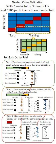
Note some previous research, including ours (Tetereva et al., 2022), splits the observations in the outer-fold training set into layer 1 and layer 2 and applies the first and second steps to layers 1 and 2, respectively. Here we decided against this approach and used the same outer-fold training set for both first and second steps in order to avoid potential bias toward the stacked models. This is because, when the data are split into two layers, predictive models built for each separate set of features only use the data from layer 1, while the stacked models use the data from both layers 1 and 2. In practice with large enough data, these two approaches might not differ much, as we demonstrated previously (Tetereva et al., 2022).
(2) I also do not feel the authors have fully addressed the concern I raised about stability of the regression coefficients over splits of the data. I wanted to see the regression coefficients, not the predictions. The predictions can be stable when the coefficients are not.
The focus of this article is on the predictions. Still, as pointed out by reviewer 1, it is informative for readers to understand how stable the feature importance (i.e., Elastic Net coefficients) is. To demonstrate the stability of feature importance, we now examined the rank stability of feature importance using Spearman’s ρ (see Figure 4). Specifically, we correlated the feature importance between two prediction models of the same features, used in two different outer-fold test sets. Given that there were five outer-fold test sets, we computed 10 Spearman’s ρ for each prediction model of the same features. We found Spearman’s ρ to be varied dramatically in both age-prediction (range=.31-.94) and fluid cognition-prediction (range=.16-.84) models. This means that some prediction models were much more stable in their feature importance than others. This is probably due to various factors such as a) the collinearity of features in the model, b) the number of features (e.g., 71,631 features in functional connectivity, which were further reduced to 75 PCAs, as compared to 19 features in subcortical volume based on the ASEG atlas), c) the penalisation of coefficients either with ‘Ridge’ or ‘Lasso’ methods, which resulted in reduction as a group of features or selection of a feature among correlated features, respectively, and d) the predictive performance of the models. Understanding the stability of feature importance is beyond the scope of the current article. As mentioned by Reviewer 1, “The predictions can be stable when the coefficients are not,” and we chose to focus on the prediction in the current article.
Author response image 2.
Stability of feature importance (i.e., Elastic Net Coefficients) of prediction models. Each dot represents rank stability (reflected by Spearman’s ρ) in the feature importance between two prediction models of the same features, used in two different outer-fold test sets. Given that there were five outer-fold test sets, there were 10 Spearman’s ρs for each prediction model. The numbers to the right of the plots indicate the mean of Spearman’s ρ for each prediction model.
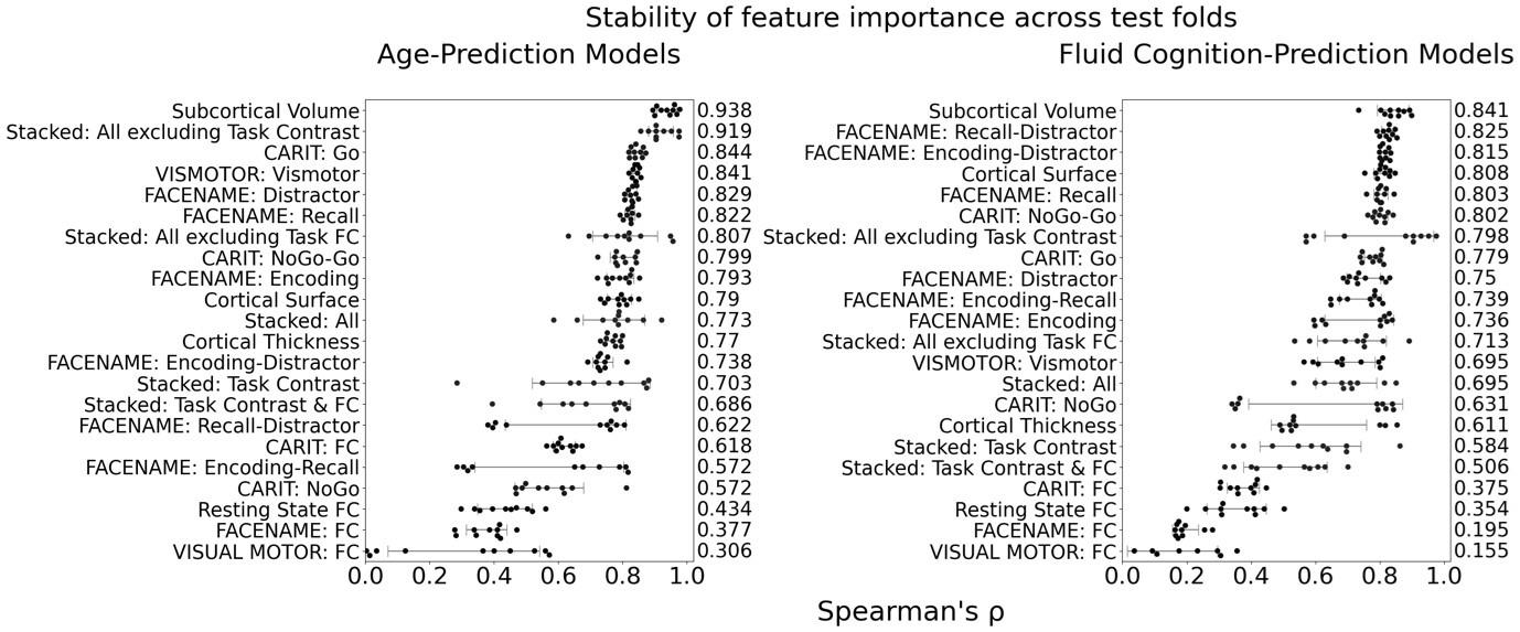
(3) I also must say that I agree with Reviewer 3 about the limitations of the brain-age and brain-cognition methods conceptually. In particular that the regression model used to predict fluid cognition will by construction explain more variance in cognition than a brain-age model that is trained to predict age. This suffers from the same problem the authors raise with brain-age and I agree that this would probably disappear if the authors had a separate measure of cognition against which to validate and were then to regress this out as they do for age correction. I am aware that these conceptual problems are more widespread than this paper alone (in fact throughout the brain-age literature), so I do not believe the authors should be penalised for that. However, I do think they can make these concerns more explicit and further tone down the comments they make about the utility of brain-cognition.
Thank you so much for raising this point. Reviewer 2 (Public Review #1) and Reviewer 3 (Recommendations for the Authors #1) made a similar observation. We now made changes to the introduction and discussion to address this concern (see below).
Briefly, we made it explicit that, by design, the variation in fluid cognition explained by Brain Cognition should be higher or equal to that explained by Brain Age. That is, the relationship between Brain Cognition and fluid cognition indicates the upper limit of Brain Age’s capability in capturing fluid cognition. More importantly, by examining what was captured by Brain Cognition, over and above Brain Age and chronological age via the unique effects of Brain Cognition, we were able to quantify the amount of co-variation between brain MRI and fluid cognition that was missed by Brain Age. And this is the third goal of this present study.
From Introduction:
“Third and finally, certain variation in fluid cognition is related to brain MRI, but to what extent does Brain Age not capture this variation? To estimate the variation in fluid cognition that is related to the brain MRI, we could build prediction models that directly predict fluid cognition (i.e., as opposed to chronological age) from brain MRI data. Previous studies found reasonable predictive performances of these cognition-prediction models, built from certain MRI modalities (Dubois et al., 2018; Pat et al., 2022; Rasero et al., 2021; Sripada et al., 2020; Tetereva et al., 2022; for review, see Vieira et al., 2022). Analogous to Brain Age, we called the predicted values from these cognition-prediction models, Brain Cognition. The strength of an out-of-sample relationship between Brain Cognition and fluid cognition reflects variation in fluid cognition that is related to the brain MRI and, therefore, indicates the upper limit of Brain Age’s capability in capturing fluid cognition. This is, by design, the variation in fluid cognition explained by Brain Cognition should be higher or equal to that explained by Brain Age. Consequently, if we included Brain Cognition, Brain Age and chronological age in the same model to explain fluid cognition, we would be able to examine the unique effects of Brain Cognition that explain fluid cognition beyond Brain Age and chronological age. These unique effects of Brain Cognition, in turn, would indicate the amount of co-variation between brain MRI and fluid cognition that is missed by Brain Age.”
From Discussion:
“Third, by introducing Brain Cognition, we showed the extent to which Brain Age indices were not able to capture the variation in fluid cognition that is related to brain MRI. More specifically, using Brain Cognition allowed us to gauge the variation in fluid cognition that is related to the brain MRI, and thereby, to estimate the upper limit of what Brain Age can do. Moreover, by examining what was captured by Brain Cognition, over and above Brain Age and chronological age via the unique effects of Brain Cognition, we were able to quantify the amount of co-variation between brain MRI and fluid cognition that was missed by Brain Age.
From our results, Brain Cognition, especially from certain cognition-prediction models such as the stacked models, has relatively good predictive performance, consistent with previous studies (Dubois et al., 2018; Pat et al., 2022; Rasero et al., 2021; Sripada et al., 2020; Tetereva et al., 2022; for review, see Vieira et al., 2022). We then examined Brain Cognition using commonality analyses (Nimon et al., 2008) in multiple regression models having a Brain Age index, chronological age and Brain Cognition as regressors to explain fluid cognition. Similar to Brain Age indices, Brain Cognition exhibited large common effects with chronological age. But more importantly, unlike Brain Age indices, Brain Cognition showed large unique effects, up to around 11%. As explained above, the unique effects of Brain Cognition indicated the amount of co-variation between brain MRI and fluid cognition that was missed by a Brain Age index and chronological age. This missing amount was relatively high, considering that Brain Age and chronological age together explained around 32% of the total variation in fluid cognition. Accordingly, if a Brain Age index was used as a biomarker along with chronological age, we would have missed an opportunity to improve the performance of the model by around one-third of the variation explained.”
Reviewer #3 (Recommendations For The Authors):
Thank you to the authors for addressing so many of my concerns with this revision. There are a few points that I feel still need addressing/clarifying related to: 1) calculating brain cognition, 2) the inevitability of their results, and 3) their continued recommendation to use brain age metrics.
(1) I understand your point here. I think the distinction is that it is fine to build predictive models, but then there is no need to go through this intermediate step of "brain-cognition". Just say that brain features can predict cognition XX well, and brain-age (or some related metric) can predict cognition YY well. It creates a confusing framework for the reader that can lead them to believe that "brain-cognition" is not just a predicted value of fluid cognition from a model using brain features to predict cognition. While you clearly state that that is in fact what it is in the text, which is a huge improvement, I do not see what is added by going through brain-cognition instead of simply just obtaining a change in R2 where the first model uses brain features alone to predict cognition, and the second adds on brain-age (or related metrics), or visa versa, depending on the question. Please do this analysis, and either compare and contrast it with going through "brain-cognition" in your paper, or switch to this analysis, as it more directly addresses the question of the incremental predictive utility of brain-age above and beyond brain features.
Thank you so much for raising this point. Reviewer 1 (Public Review #2/Recommendations For The Authors #3) and Reviewer 2 (Public Review #1) made a similar observation. We now made changes to the introduction and discussion to address this concern (see our responses to Reviewer 1 Recommendations For The Authors #3 above).
Briefly, as in our 2nd revision, we made it explicitly clear that we did not intend to compare Brain Age with Brain Cognition since, by design, the variation in fluid cognition explained by Brain Cognition should be higher or equal to that explained by Brain Age. And, by examining what was captured by Brain Cognition, over and above Brain Age and chronological age via the unique effects of Brain Cognition, we were able to quantify the amount of co-variation between brain MRI and fluid cognition that was missed by Brain Age.
We have thought about changing the name Brain Cognition into something along the lines of “predicted values of prediction models predicting fluid cognition based on brain MRI.” However, this made the manuscript hard to follow, especially with the commonality analyses. For instance, the sentence, “Here, we tested Brain Cognition’s unique effects in multiple regression models with a Brain Age index, chronological age and Brain Cognition as regressors to explain fluid cognition” would become “Here, we tested predicted values of prediction models predicting fluid cognition based on brain MRI unique effects in multiple regression models with a Brain Age index, chronological age and predicted values of prediction models predicting fluid cognition based on brain MRI as regressors to explain fluid cognition.” We believe, given our additional explanation (see our responses to Reviewer 1 Recommendations For The Authors #3 above), readers should understand what Brain Cognition is, and that we did not intend to compare Brain Age and Brain Cognition directly.
As for the suggested analysis, “obtaining a change in R2 where the first model uses brain features alone to predict cognition, and the second adds on brain-age (or related metrics), or visa versa,” we have already done this in the form of commonality analysis (Nimon et al., 2008) (see Figure 7 below). That is, to obtain unique and common effects of the regressors, we need to look at all of the possible changes in R2 when all possible subsets of regressors were excluded or included, see equations 12 and 13 below.
From Methods:
“Similar to the above multiple regression model, we had chronological age, each Brain Age index and Brain Cognition as the regressors for fluid cognition:
Fluid Cognitioni = β0 + β1 Chronological Agei + β2 Brain Age Indexi,j + β3 Brain Cognitioni + εi, (12)
Applying the commonality analysis here allowed us, first, to investigate the addictive, unique effects of Brain Cognition, over and above chronological age and Brain Age indices. More importantly, the commonality analysis also enabled us to test the common, shared effects that Brain Cognition had with chronological age and Brain Age indices in explaining fluid cognition. We calculated the commonality analysis as follows (Nimon et al., 2017):
Unique Effectchronological age = ΔR2chronological age = R2chronological age, Brain Age index, Brain Cognition – R2 Brain Age index, Brain Cognition
Unique EffectBrain Age index = ΔR2Brain Age index = R2chronological age, Brain Age index, Brain Cognition – R2 chronological age, Brain Cognition
Unique EffectBrain Cognition = ΔR2Brain Cognition = R2chronological age, Brain Age index, Brain Cognition – R2 chronological age, Brain Age Index
Common Effectchronological age, Brain Age index = R2chronological age, Brain Cognition + R2 Brain Age index, Brain Cognition – R2 Brain Cognition – R2chronological age, Brain Age index, Brain Cognition
Common Effectchronological age, Brain Cognition = R2chronological age, Brain Age Index + R2 Brain Age index, Brain Cognition – R2 Brain Age Index – R2chronological age, Brain Age index, Brain Cognition
Common Effect Brain Age index, Brain Cognition = R2chronological age, Brain Age Index + R2 chronological age, Brain Cognition – R2 chronological age – R2chronological age, Brain Age index, Brain Cognition
Common Effect chronological age, Brain Age index, Brain Cognition = R2 chronological age + R2 Brain Age Index + R2 Brain Cognition – R2chronological age, Brain Age Index – R2 chronological age, Brain Cognition – R2 Brain Age Index, Brain Cognition – R2chronological age, Brain Age index, Brain Cognition , (13)”
(2) I agree that the solution is not to exclude age as a covariate, and that there is a big difference between inevitable and obvious. I simply think a further discussion of the inevitability of the results would be clarifying for the readers. There is a big opportunity in the brain-age literature to be as direct as possible about why you are finding what you are finding. People need to know not only what you found, but why you found what you found.
Thank you. We agreed that we need to make this point more explicit and direct. In the revised manuscript, we had the statements in both Introduction and Discussion (see below) about the tight relationship between Brain Age and chronological age by design, making the small unique effects of Brain Age inevitable.
Introduction:
“Accordingly, by design, Brain Age is tightly close to chronological age. Because chronological age usually has a strong relationship with fluid cognition, to begin with, it is unclear how much Brain Age adds to what is already captured by chronological age.“
Discussion:
“First, Brain Age itself did not add much more information to help us capture fluid cognition than what we had already known from a person’s chronological age. This can clearly be seen from the small unique effects of Brain Age indices in the multiple regression models having Brain Age and chronological age as the regressors. While the unique effects of some Brain Age indices from certain age-prediction models were statistically significant, there were all relatively small. Without Brain Age indices, chronological age by itself already explained around 32% of the variation in fluid cognition. Including Brain Age indices only added around 1.6% at best. We believe the small unique effects of Brain Age were inevitable because, by design, Brain Age is tightly close to chronological age. Therefore, chronological age and Brain Age captured mostly a similar variation in fluid cognition.
Investigating the simple regression models and the commonality analysis between each Brain Age index and chronological age provided additional insights….”
(3) I believe it is very important to critically examine the use of brain-age and related metrics. As part of this process, I think we should be asking ourselves the following questions (among others): Why go through age prediction? Wouldn't the predictions of cognition (or another variable) using the same set of brain features always be as good or better? You still have not justified the use of brain-age. As I said before, if you are going to continue to recommend the use of brain-age, you need a very strong argument for why you are recommending this. What does it truly add? Otherwise, temper your statements to indicate possible better paths forward.
Thank you Reviewer 3 for making an argument against the use of Brain Age. We largely agree with you. However, our work only focuses on one phenotype, fluid cognition, and on the normative situation (i.e., not having a case vs control group). As Reviewer 2 pointed out, Brain Age might still have utility in other cases, not studied here. Still, future studies that focus on other phenotypes may consider using our approach as a template to test the utility of Brain Age in other situations. We added the conclusion statement to reflect this.
From Discussion:
“Altogether, we examined the utility of Brain Age as a biomarker for fluid cognition. Here are the three conclusions. First, Brain Age failed to add substantially more information over and above chronological age. Second, a higher ability to predict chronological age did not correspond to a higher utility to capture fluid cognition. Third, Brain Age missed up to around one-third of the variation in fluid cognition that could have been explained by brain MRI. Yet, given our focus on fluid cognition, future empirical research is needed to test the utility of Brain Age on other phenotypes, especially when Brain Age is used for anomaly detection in case-control studies (e.g., Bashyam et al., 2020; Rokicki et al., 2021). We hope that future studies may consider applying our approach (i.e., using the commonality analysis that includes predicted values from a model that directly predicts the phenotype of interest) to test the utility of Brain Age as a biomarker for other phenotypes.”
References
Bashyam, V. M., Erus, G., Doshi, J., Habes, M., Nasrallah, I. M., Truelove-Hill, M., Srinivasan, D., Mamourian, L., Pomponio, R., Fan, Y., Launer, L. J., Masters, C. L., Maruff, P., Zhuo, C., Völzke, H., Johnson, S. C., Fripp, J., Koutsouleris, N., Satterthwaite, T. D., … on behalf of the ISTAGING Consortium, the P. A. disease C., ADNI, and CARDIA studies. (2020). MRI signatures of brain age and disease over the lifespan based on a deep brain network and 14 468 individuals worldwide. Brain, 143(7), 2312–2324. https://doi.org/10.1093/brain/awaa160
Butler, E. R., Chen, A., Ramadan, R., Le, T. T., Ruparel, K., Moore, T. M., Satterthwaite, T. D., Zhang, F., Shou, H., Gur, R. C., Nichols, T. E., & Shinohara, R. T. (2021). Pitfalls in brain age analyses. Human Brain Mapping, 42(13), 4092–4101. https://doi.org/10.1002/hbm.25533
Cole, J. H. (2020). Multimodality neuroimaging brain-age in UK biobank: Relationship to biomedical, lifestyle, and cognitive factors. Neurobiology of Aging, 92, 34–42. https://doi.org/10.1016/j.neurobiolaging.2020.03.014
Dubois, J., Galdi, P., Paul, L. K., & Adolphs, R. (2018). A distributed brain network predicts general intelligence from resting-state human neuroimaging data. Philosophical Transactions of the Royal Society B: Biological Sciences, 373(1756), 20170284. https://doi.org/10.1098/rstb.2017.0284
Hahn, T., Fisch, L., Ernsting, J., Winter, N. R., Leenings, R., Sarink, K., Emden, D., Kircher, T., Berger, K., & Dannlowski, U. (2021). From ‘loose fitting’ to high-performance, uncertainty-aware brain-age modelling. Brain, 144(3), e31–e31. https://doi.org/10.1093/brain/awaa454
Insel, T., Cuthbert, B., Garvey, M., Heinssen, R., Pine, D. S., Quinn, K., Sanislow, C., & Wang, P. (2010). Research Domain Criteria (RDoC): Toward a New Classification Framework for Research on Mental Disorders. American Journal of Psychiatry, 167(7), 748–751. https://doi.org/10.1176/appi.ajp.2010.09091379
Jirsaraie, R. J., Kaufmann, T., Bashyam, V., Erus, G., Luby, J. L., Westlye, L. T., Davatzikos, C., Barch, D. M., & Sotiras, A. (2023). Benchmarking the generalizability of brain age models: Challenges posed by scanner variance and prediction bias. Human Brain Mapping, 44(3), 1118–1128. https://doi.org/10.1002/hbm.26144
Marquand, A. F., Rezek, I., Buitelaar, J., & Beckmann, C. F. (2016). Understanding Heterogeneity in Clinical Cohorts Using Normative Models: Beyond Case-Control Studies. Biological Psychiatry, 80(7), 552–561. https://doi.org/10.1016/j.biopsych.2015.12.023
Nimon, K., Lewis, M., Kane, R., & Haynes, R. M. (2008). An R package to compute commonality coefficients in the multiple regression case: An introduction to the package and a practical example. Behavior Research Methods, 40(2), 457–466. https://doi.org/10.3758/BRM.40.2.457
Pat, N., Wang, Y., Anney, R., Riglin, L., Thapar, A., & Stringaris, A. (2022). Longitudinally stable, brain‐based predictive models mediate the relationships between childhood cognition and socio‐demographic, psychological and genetic factors. Human Brain Mapping, hbm.26027. https://doi.org/10.1002/hbm.26027
Poldrack, R. A., Huckins, G., & Varoquaux, G. (2020). Establishment of Best Practices for Evidence for Prediction: A Review. JAMA Psychiatry, 77(5), 534–540. https://doi.org/10.1001/jamapsychiatry.2019.3671
Rasero, J., Sentis, A. I., Yeh, F.-C., & Verstynen, T. (2021). Integrating across neuroimaging modalities boosts prediction accuracy of cognitive ability. PLOS Computational Biology, 17(3), e1008347. https://doi.org/10.1371/journal.pcbi.1008347
Rokicki, J., Wolfers, T., Nordhøy, W., Tesli, N., Quintana, D. S., Alnæs, D., Richard, G., de Lange, A.-M. G., Lund, M. J., Norbom, L., Agartz, I., Melle, I., Nærland, T., Selbæk, G., Persson, K., Nordvik, J. E., Schwarz, E., Andreassen, O. A., Kaufmann, T., & Westlye, L. T. (2021). Multimodal imaging improves brain age prediction and reveals distinct abnormalities in patients with psychiatric and neurological disorders. Human Brain Mapping, 42(6), 1714–1726. https://doi.org/10.1002/hbm.25323
Sripada, C., Angstadt, M., Rutherford, S., Taxali, A., & Shedden, K. (2020). Toward a “treadmill test” for cognition: Improved prediction of general cognitive ability from the task activated brain. Human Brain Mapping, 41(12), 3186–3197. https://doi.org/10.1002/hbm.25007
Tetereva, A., Li, J., Deng, J. D., Stringaris, A., & Pat, N. (2022). Capturing brain‐cognition relationship: Integrating task‐based fMRI across tasks markedly boosts prediction and test‐retest reliability. NeuroImage, 263, 119588. https://doi.org/10.1016/j.neuroimage.2022.119588
Vieira, B. H., Pamplona, G. S. P., Fachinello, K., Silva, A. K., Foss, M. P., & Salmon, C. E. G. (2022). On the prediction of human intelligence from neuroimaging: A systematic review of methods and reporting. Intelligence, 93, 101654. https://doi.org/10.1016/j.intell.2022.101654
Author response:
The following is the authors’ response to the previous reviews.
eLife assessment
This study presents valuable data on the antigenic properties of neuraminidase proteins of human A/H3N2 influenza viruses sampled between 2009 and 2017. The antigenic properties are found to be generally concordant with genetic groups. Additional analysis have strengthened the revised manuscript, and the evidence supporting the claims is solid.
Public Reviews:
Reviewer #1 (Public Review):
Summary
The authors investigated the antigenic diversity of recent (2009-2017) A/H3N2 influenza neuraminidases (NAs), the second major antigenic protein after haemagglutinin. They used 27 viruses and 43 ferret sera and performed NA inhibition. This work was supported by a subset of mouse sera. Clustering analysis determined 4 antigenic clusters, mostly in concordance with the genetic groupings. Association analysis was used to estimate important amino acid positions, which were shown to be more likely close to the catalytic site. Antigenic distances were calculated and a random forest model used to determine potential important sites.
This revision has addressed many of my concerns of inconsistencies in the methods, results and presentation. There are still some remaining weaknesses in the computational work.
Strengths
(1) The data cover recent NA evolution and a substantial number (43) of ferret (and mouse) sera were generated and titrated against 27 viruses. This is laborious experimental work and is the largest publicly available neuraminidase inhibition dataset that I am aware of. As such, it will prove a useful resource for the influenza community.
(2) A variety of computational methods were used to analyse the data, which give a rounded picture of the antigenic and genetic relationships and link between sequence, structure and phenotype.
(3) Issues raised in the previous review have been thoroughly addressed.
Weaknesses
(1). Some inconsistencies and missing data in experimental methods Two ferret sera were boosted with H1N2, while recombinant NA protein for the others. This, and the underlying reason, are clearly explained in the manuscript. The authors note that boosting with live virus did not increase titres. Additionally, one homologous serum (A/Kansas/14/2017) was not generated, although this would not necessarily have impacted the results.
We agree with the reviewer and this point was addressed in the previous rebuttal.
(2) Inconsistency in experimental results
Clustering of the NA inhibition results identifies three viruses which do not cluster with their phylogenetic group. Again this is clearly pointed out in the paper and is consistent with the two replicate ferret sera. Additionally, A/Kansas/14/2017 is in a different cluster based on the antigenic cartography vs the clustering of the titres
We agree with the reviewer and this point was addressed in the previous rebuttal.
(3) Antigenic cartography plot would benefit from documentation of the parameters and supporting analyses
a. The number of optimisations used
We used 500 optimizations. This information is now included in the Methods section.
b. The final stress and the difference between the stress of the lowest few (e.g. 5) optimisations, or alternatively a graph of the stress of all the optimisations. Information on the stress per titre and per point, and whether any of these were outliers
The stress was obtained from 1, 5, 500, or even 5000 optimizations (resulting in stress values of respectively, 1366.47, 1366.47, 2908.60, and 3031.41). Besides limited variation or non-conversion of the stress values after optimization, the obtained maps were consistent in multiple runs. The map was obtained keeping the best optimization (stress value 1366.47, selected using the keepBestOptimization() function).
Author response image 1.
The stress per point is presented in the heat map below.
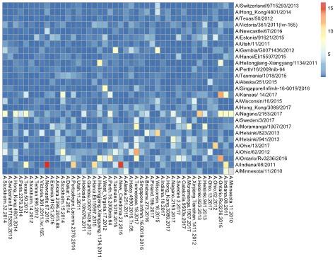
The heat map indicates stress per serum (x-axis) and strain (y-axis) in blue to red scale.
c. A measure of uncertainty in position (e.g. from bootstrapping)
Bootstrap was performed using 1000 repeats and 100 optimizations per repeat. The uncertainty is represented in the blob plot below.
Author response image 2.
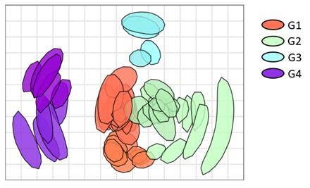
(4) Random forest
The full dataset was used for the random forest model, including tuning the hyperparameters. It is more robust to have a training and test set to be able to evaluate overfitting (there are 25 features to classify 43 sera).
Explicit cross validation is not necessary for random forests as the out of bag process with multiple trees implicitly covers cross validation. In the random forest function in R this is done by setting the mtry argument (number of variables randomly sampled as candidates at each split). R samples variables with replacement (the same variable can be sampled multiple times) of the candidates from the training set. RF will then automatically take the data that is not selected as candidates as test set. Overfit may happen when all data is used for training but the RF method implicitly does use a test set and does not use all data for training.
Code:
rf <- randomForest(X,y=Y,ntree=1500,mtry=25,keep.forest=TRUE,importance=TRUE)
Reviewer #2 (Public Review):
Summary:
The authors characterized the antigenicity of N2 protein of 43 selected A(H3N2) influenza A viruses isolated from 2009-2017 using ferret and mice immune sera. Four antigenic groups were identified, which the authors claimed to be correlated with their respective phylogenic/ genetic groups. Among 102 amino acids differed by the 44 selected N2 proteins, the authors identified residues that differentiate the antigenicity of the four groups and constructed a machine-learning model that provides antigenic distance estimation. Three recent A(H3N2) vaccine strains were tested in the model but there was no experimental data to confirm the model prediction results.
Strengths:
This study used N2 protein of 44 selected A(H3N2) influenza A viruses isolated from 2009-2017 and generated corresponding panels of ferret and mouse sera to react with the selected strains. The amount of experimental data for N2 antigenicity characterization is large enough for model building.
Weaknesses:
The main weakness is that the strategy of selecting 43 A(H3N2) viruses from 2009-2017 was not explained. It is not clear if they represent the overall genetic diversity of human A(H3N2) viruses circulating during this time. In response to the reviewer's comment, the authors have provided a N2 phylogenetic tree using180 randomly selected N2 sequences from human A(H3N2) viruses from 2009-2017. While the 43 strains seems to scatter across the N2 tree, the four antigenic groups described by the author did not correlated with their respective phylogenic/ genetic groups as shown in Fig. 2. The authors should show the N2 phylogenic tree together with Fig. 2 and discuss the discrepancy observed.
The discrepancies between the provided N2 phylogenetic tree using 180 selected N2 sequences was primarily due to visualization. In the tree presented in Figure 2 the phylogeny was ordered according to branch length in a decreasing way. Further, the tree represented in the rebuttal was built with PhyML 3.0 using JTT substitution model, while the tree in figure 2 was build in CLC Workbench 21.0.5 using Bishop-Friday substitution model. The tree below was built using the same methodology as Figure 2, including branch size ordering. No discrepancies are observed.
Phylogenetic tree representing relatedness of N2 head domain. N2 NA sequences were ordered according to the branch length and phylogenetic clusters are colored as follows: G1: orange, G2: green, G3: blue, and G4: purple. NA sequences that were retained in the breadth panel are named according to the corresponding H3N2 influenza viruses. The other NA sequences are coded.
Author response image 3.
The second weakness is the use of double-immune ferret sera (post-infection plus immunization with recombinant NA protein) or mouse sera (immunized twice with recombinant NA protein) to characterize the antigenicity of the selected A(H3N2) viruses. Conventionally, NA antigenicity is characterized using ferret sera after a single infection. Repeated influenza exposure in ferrets has been shown to enhance antibody binding affinity and may affect the cross-reactivity to heterologous strains (PMID: 29672713). The increased cross-reactivity is supported by the NAI titers shown in Table S3, as many of the double immune ferret sera showed the highest reactivity not against its own homologous virus but to heterologous strains. In response to the reviewer's comment, the authors agreed the use of double-immune ferret sera may be a limitation of the study. It would be helpful if the authors can discuss the potential effect on the use of double-immune ferret sera in antigenicity characterization in the manuscript.
Our study was designed to understand the breadth of the anti-NA response after the incorporation of NA as a vaccine antigens. Our data does not allow to conclude whether increased breadth of protection is merely due to increased antibody titers or whether an NA boost immunization was able to induce antibody responses against epitopes that were not previously recognized by primary response to infection. However, we now mention this possibility in the discussion and cite Kosikova et al. CID 2018, in this context.
Another weakness is that the authors used the newly constructed a model to predict antigenic distance of three recent A(H3N2) viruses but there is no experimental data to validate their prediction (eg. if these viruses are indeed antigenically deviating from group 2 strains as concluded by the authors). In response to the comment, the authors have taken two strains out of the dataset and use them for validation. The results is shown as Fig. R7. However, it may be useful to include this in the main manuscript to support the validity of the model.
The removal of 2 strains was performed to illustrate the predictive performance of the RF modeling. However, Random Forest does not require cross-validation. The reason is that RF modeling already uses an out-of-bag evaluation which, in short, consists of using only a fraction of the data for the creation of the decision trees (2/3 of the data), obviating the need for a set aside the test set:
“…In each bootstrap training set, about one-third of the instances are left out. Therefore, the out-of-bag estimates are based on combining only about one- third as many classifiers as in the ongoing main combination. Since the error rate decreases as the number of combinations increases, the out-of-bag estimates will tend to overestimate the current error rate. To get unbiased out-of-bag estimates, it is necessary to run past the point where the test set error converges. But unlike cross-validation, where bias is present but its extent unknown, the out-of-bag estimates are unbiased…” from https://www.stat.berkeley.edu/%7Ebreiman/randomforest2001.pdf
Reviewer #3 (Public Review):
Summary:
This paper by Portela Catani et al examines the antigenic relationships (measured using monotypic ferret and mouse sera) across a panel of N2 genes from the past 14 years, along with the underlying sequence differences and phylogenetic relationships. This is a highly significant topic given the recent increased appreciation of the importance of NA as a vaccine target, and the relative lack of information about NA antigenic evolution compared with what is known about HA. Thus, these data will be of interest to those studying the antigenic evolution of influenza viruses. The methods used are generally quite sound, though there are a few addressable concerns that limit the confidence with which conclusions can be drawn from the data/analyses.
Strengths:
- The significance of the work, and the (general) soundness of the methods. -Explicit comparison of results obtained with mouse and ferret sera
Weaknesses:
- Approach for assessing influence of individual polymorphisms on antigenicity does not account for potential effects of epistasis (this point is acknowledged by the authors).
We agree with the reviewer and this point was addressed in the previous rebuttal.
- Machine learning analyses neither experimentally validated nor shown to be better than simple, phylogenetic-based inference.
We respectfully disagree with the reviewer. This point was addressed in the previous rebuttal as follows.
This is a valid remark and indeed we have found a clear correlation between NAI cross reactivity and phylogenetic relatedness. However, besides achieving good prediction of the experimental data (as shown in Figure 5 and in FigureR7), machine Learning analysis has the potential to rank or indicate major antigenic divergences based on available sequences before it has consolidated as new clade. ML can also support the selection and design of broader reactive antigens. “
Recommendations for the authors:
Reviewer #2 (Recommendations For The Authors):
(1) Discuss the discrepancy between Fig. 2 and the newly constructed N2 phylogenetic tree with 180 randomly selected N2 sequences of A(H3N2) viruses from 2009-2017. Specifically please explain the antigenic vs. phylogenetic relationship observed in Fig. 2 was not observed in the large N2 phylogenetic tree.
Discrepancies were due to different method and visualization. A new tree was provided.
(2) Include a sentence to discuss the potential effect on the use of double-immune ferret sera in antigenic characterization.
We prefer not to speculate on this.
(3) Include the results of the exercise run (with the use of Swe17 and HK17) in the manuscript as a way to validate the model.
The exercise was performed to illustrate predictive potential of the RF modeling to the reviewer. However, cross-validation is not a usual requirement for random forest, since it uses out-of-bag calculations. We prefer to not include the exercise runs within the main manuscript.
Author Response
The following is the authors’ response to the original reviews.
Reviewer #1 (Recommendations for The Authors):
To hopefully contribute to more strongly support the conclusions of the manuscript, I am including a series of concerns regarding the experiments, as well as some recommendations that could be followed to address these issues:
(1) The Q-nMT bundle is largely unaffected by the nocodazole treatment in most phases during its formation. However, cells were only treated with nocodazole for a very short period of time (15 min). Have the authors analyzed Q-nMT stability after longer nocodazole exposures? Is a similar treatment enough to depolymerize the mitotic spindle? This result could be further substantiated by treatment with other MT-depolymerizing agents. Furthermore, the dynamicity of the Q-nMT bundle could be ideally also assessed by other techniques, such as FRAP.
The experiments suggested by the reviewer have been published in our previous paper (Laporte et al, JCB 2013). In this previous study, we presented data demonstrating the resistance of the Q-nMT bundle to several MT poisons: TBZ, benomyl, MBC (Sup Fig 2D) and to an increasing amount of nocodazole after a 90 min treatment (Sup Fig2E). These published figures are provided below.
Author response image 1.
The nMT array contains highly stable MTS. (A) Variation Of nuclear MT length in function Of time (second) in proliferating cells. Cells express GFP•Tubl (green) and Nup2•RFP (red). Bars, 2 pm. N = l, n is indicated. (B) Variation of the nMT array length in function of time measured for BirnlGFP—expressing cells In = 161, for 6-d•old Dad2GFP—expressing cells In = 171, for Stu2GFP—expressing cells (n = 17), and 6•d-old Nuf2• GFP—expressing cells (n = 17). Examples Of corresponding time lapse are shown. Time is in minutes experiments). Bar, 2 pm. (CJ Nuf2•GFP dots detected along nMT array (arrow) are immobile. Several time lapse images of cells are shown. Time is in minutes. gar, 2 pm _ MT organizations in proliferating cells and 4-d•old quiescent cells before and after a 90-min treatment With indicated drugs. Bar, 2 pm. (E) MT organizations in Sci-old quiescent cells before and after a 90min treatment With increasing concentrations Of nocodazole.
In the same article, we showed that Q-nMT bundles resist a 3h nocodazole treatment, while all MT structures assembled in proliferating cells, including mitotic spindle, vanished (see Fig 2E below). In addition, in our previous article, FRAP experiments were provided in Fig 2D.
Author response image 2.
The nuclear array is composed of stable MTS. Variation of the length in function of time of (A) aMTs in proliferating cells, (B) nMT array in quiescent cells (7 d), and the two MT structures in early quiescent cells (4 d). White arrows point ot dynamic aMTs. In A—C, N = 2, n is indicated ID) FRAP on 7-d-old quiescent cells. White arrows point to bleach areas. Error bars are SEM. In A—D. time is in seconds. (E) nMT array is not affected by nocodazole treatment. Before and various times after carbon exhaustion (red dashed line), cells were incubated for 3 h with 22.5 pg/pL nocodozole and then imaged. The corresponding control experiment is shown in Fig I A. In all panels, cells expressing GFP-TtJbl (green) and Nup2-RFP (red) are shown; bars, 2 pm.
This previous study was mentioned in the introduction and is now re-cited at the beginning of the results section (line 107-108).
As expected from our previous study, when proliferating cells were treated with Noc (30 µg/ml) in the same conditions as in Fig1, most of the short and the long mitotic spindles vanished after a 15 min treatment as shown in the graph below.
Author response image 3.
Proliferating cells expressing NOf2=GFP and mTQZ-TUb1 (00—2) were treated or not With NOC (30vgfmI) for 15 min.% Of cells With detectable MT and representative cells are shown. Khi-teet values are indicated. Bar: 2 pm,
(2) The graph in Figure 1B is somewhat confusing. Is the X-axis really displaying the length of the MTs as stated in the legend? If so, one would expect to see a displacement of the average MT length of the population as cells progress from phase II to phase III, as previously demonstrated in Figure 1A. Likewise, no data points would be anticipated for those phases in which the MT length is 0 or close to 0. Moreover, when the length of half pre-anaphase mitotic spindle was measured as a control, how can one get MT lengths that are equal or close to 0 in these cells? The length of the pre-anaphase spindle is between 2-4 um, so MT length values should range from 1 to 2 um if half the spindle is measured.
The graph in Fig1B represents the fluorescence intensity (a proxy for the Q-nMT bundle thickness) along the Q-nMT bundle length.
Fluorescence intensity is measured along a “virtual line” that starts 0,5 µm before the extremity of the QnMT bundle that is in contact with the SPB. In other words, we aligned all intensity measurements at the fluorescence increasing onset on the SPB side. We arbitrarily set the ‘zero’ at 0,5um before the fluorescence increased onset. That is why the fluorescence intensity is zero between 0 and 0,5 µm – The X-axis represents this virtual line, the 0 being set 0,5 µm before the Q-nMT bundle extremity on the SPB side. This virtual line allows us to standardize our “thickness” measurements for all Q-nMT bundles.
Using this standardization, it is clear that the length of the Q-nMT bundles increased from phase II to III (see the red arrow). Yet, as in phase II, Q-nMT bundles are not yet stable, their lengths are shorter in phase II than in phase II after a Noc treatment (compare the end of the orange line and the end of the blue line in phase II).
Author response image 4.
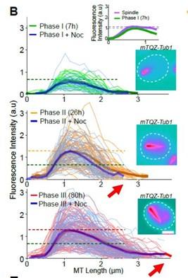
This is now explained in details in the Material and Methods section (line 539-545).
This is the same for the inset of Fig 1B and in Sup Fig 1A, in which we measured fluorescence intensity along the halfmitotic spindle just as we did for MT bundle. The X-axis represent a virtual line along the mitotic spindle, starting 0,5 µm before the SBP spindle extremity.
Author response image 5.
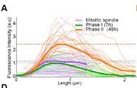
(3) Microtubules seem to locate next to or to extend beyond the nucleus in the control cells (DMSO) in Figure 1H. Since both nuclear MTs and cytoplasmic MTs emanate from the SPBs, it would have been desirable to display the morphology of the nucleus when possible. Moreover, since the nucleus is a tridimensional structure, it would also be advisable to image different Z-sections.
Analysis demonstrating that Q-nMT bundles are located inside the nucleus have been provided in our previous paper (Laporte et al, JCB 2013). In this article most of the images are maximal projections of Z-stacks in which the nuclear envelope is visualized via Nup2-RFP (see Fig1 of Laporte et al, JCB 2013 as an example below).
Author response image 6.
MTsare organized as a nuclear array in quiescent cells. (A) MT reorganization upon quiescence entry. Cells expressing GFP-Tub1 (green) and Nup2RFP (red) are shown. Glucose exhaustion is indicated as a red dashed line. Quiescent cells dl expressing Tub I-RFP and either Spc72GFP,
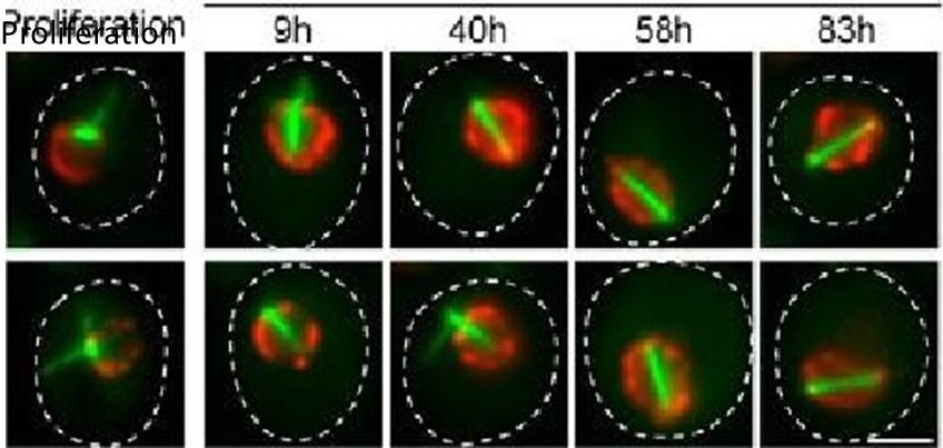
In Laporte et al, JCB 2013, we also provided EM analysis both in cryo and immune-gold (Fig 1E below).
Author response image 7.
(top) or coexpr;sse8 with Tub I-RFP (bottom). Arrows point dot along the nMT array. Bars: (A—C)) 2 pm. (E) AMT arroy visualized in WT cells by EMI Yellow arrows, MTS; red arrowheads, nuclear membrane; pink arrow, SPB. Insets: nMT cut transversally. Bar, 100 nm.
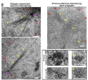
(4) Movies depicting the process of Q-nMT bundle formation in live cells would have been really informative to more precisely evaluate the MT dynamics. Likewise, together with still images (Fig 1D and Supp. Fig. 1D), movies depicting the changes in the localization of Nuf2-GFP would have further facilitated the analysis of this process.
In a new Sup Fig 1E, we now provide images of Q-nMT bundle formation initiation in phase I, in which it can be observed that Nuf2-GFP accompanies the growth of MT (mTQZ-TUB1) at the onset of Q-nMT bundle formation. Unfortunately, it is technically very challenging to follow the entire process of Q-nMT bundle formation in individual cells, as it takes > 48h. Indeed, for movies longer than 24h, on both microscope pads or specific microfluidic devices (Jacquel, et al, eLife 2021), phototoxicity and oxygen availability become problematic and affect cells’ viability.
(5) Western blot images displaying the relative protein levels for mTQZ-Tub1 and of the ADH2 promoter-driven mRuby-Tub1 at the different time points should be included to more strongly support the conclusion that new tubulin molecules are introduced in the Q-nMT bundle only after phase I. It is worth noting, in this sense, that the percentage of cells with 2 colors Q-nMT bundle is analyzed only 1 hour after expression of mRuby-Tub1 was induced for phase I cells, but after 24 hours for phase II cells.<br /> We have modified Fig 1F and now provide images of cells after 3, 6 and 24h after glucose exhaustion and the corresponding percentage of cells displaying Q-nMT bundle with the two colors. We also now provide a western blot in Sup Fig 1H using specific antibodies against mTQZ (anti-GFP) and mRuby (anti-RFP).
(6) In order to demonstrate that Q-nMT formation is an active process induced by a transient signal and that the Q-nMT bundle is required for cell survival, the authors treated cells with nocodazole for 24 h (Fig 1H and Supp Fig 1K). Both events, however, could be associated with the toxic effects of the extremely prolonged nocodazole treatment leading to cell death.
We have treated 5 days old cells for 24h with 30 µg/ml Noc. We then washed the drug and transferred the cells into a glucose free medium. We then followed both cell survival, using methylene blue, and the cell’s capacity to form a colony after refeeding. In these conditions, we did not observe any toxic effect of the nocodazole. This result is now provided in Sup Fig 1L and discussed line 172-176.
(7) The "Tub1-only" mutant displays shorter but stable Q-nMT bundles in phase II, although they are thinner than in wild-type cells. What happens in the "Tub3-only" mutant, which also has beta-tubulin levels similar to wild-type cells (Supp. Fig. 2B)?
In order to measure Q-nMT bundle length and thickness, we used Tub1 fused to GFP. This cannot be done in a Tub3-only mutant. Yet, we have measured Q-nMT bundle length in Tub3-only cells using Bim1-3GFP as a MT marker (as in Laporte et al, JCB 2013). As shown in the figure below, Q-nMT bundles were shorter in Tub3-only cells than in WT cells whatever the phase.
Author response image 8.
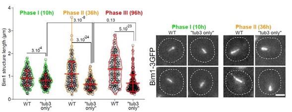
We do not know if this effect is directly linked to the absence of Tub1 or if it is very indirect and for example due to the fact that Tub1 and Tub3 interact differently with Bim1 or other proteins that are involved in Q-nMT bundle stabilization. As we cannot give a clear interpretation for that result, we decided not to present those data in our manuscript.
(8) Why were wild-type and ndc80-1 cells imaged after a 20 min nocodazole treatment to evaluate the role of KT-MT attachments in Q-nMT bundle formation (Fig 3A)? Importantly, this experiment is also missing a control in which Q-nMT length is analyzed in both wild-type and ndc80-1 cells at 25ºC instead of 37ºC.
In this experiment, we used nocodazole to test both the formation and the stability of the Q-nMT bundle. Fig 3A shows MT length distribution in WT (grey) and ndc80-1 (violet) cells expressing mTQZTub1 (green) and Nuf2-GFP (red), shifted to 37 °C at the onset of glucose exhaustion and kept at this non-permissive temperature for 12 or 96 h then treated with Noc. The control experiment was provided in Sup Fig 3B. Indeed, this figure shows MT length in WT (grey) and ndc80-1 (violet) expressing mTQZ-Tub1 (green) and Nuf2-GFP (red) grown for 4 d (96h) at 25 °C, and treated or not with Noc. This is now indicated in the text line 216 and in the figure legend line 976
Author response image 9.
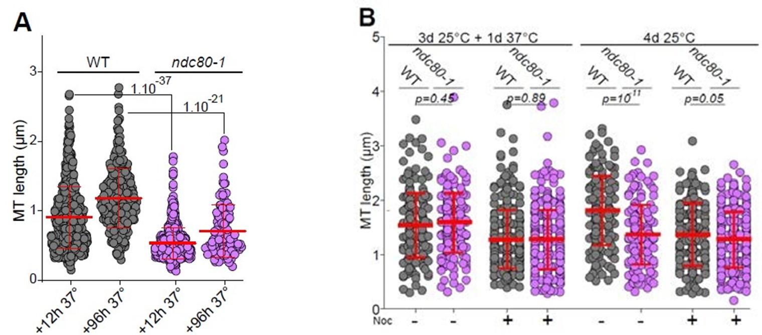
(9) As a general comment linked to the previous concern, it is striking that in many instances, Q-nMT bundle length is measured after nocodazole treatment without any evident reason to do this and without displaying the results in untreated cells as a control. If nocodazole is used, the authors should explicitly indicate it and state the reason for it.
We provide control experiments without nocodazole for all of the figures. For the sake of figure clarity, for Fig.3A the control without the drug is in Sup. Fig. 3B, for Fig. 3B it is shown in Sup. Fig. 3D, for Fig. 4B, it is shown in Sup. Fig 4A. This is now stated in the text and in the figure legend: for Fig. 3A: line 216 and in the figure legend line 976; for Fig. 3B: line 222 and figure legend line 984; for Fig. 4B: line 280 and in the figure legend line 1017.
The only figures where the untreated cells are not shown is for Fig 1D since the goal of the experiment is to make dynamic MTs shorten.
In Fig. 5C and Sup. Fig. 5D to F, we used nocodazole to get rid of dynamic cytoplasmic MTs that form upon quiescence exit in order to facilitate Q-nMT bundle measurement. This was explained in our previous study (Laporte et al, JCB 2013). We now mention it in the figure legends, see for example Fig. 5 legend line 1054.
(10) Ipl1 inactivation using the ipl1-1 thermosensitive allele impedes Q-nMT bundle formation. The inhibitor-sensitive ipl1-as1 allele could have been further used to show whether this depends on its kinase activity, also avoiding the need to increase the temperature, which affects MT dynamics. As suggested, we have used the ipl1-5as allele. We have thus modified Fig 3B and now show that is it indeed the Ipl1 kinase activity that is required for Q-nMT bundle formation initiation (line 222). In any case, it is surprising that deletion of SLI15 does not affect Q-nMT formation (in fact, MT length is even larger), despite the fact that Sli15, which localizes and activates Ipl1, is present at the Q-nMT (Fig 3C). Likewise, deletion of BIR1 has barely any effect on MT length after 4 days in quiescence (Fig 3D). Do the previous observations mean that Ipl1 role is CPC-independent? Does the lack of Sli15 or Bir1 aggravate the defect in Q-nMT formation of ipl1-1 cells at non-permissive or semi-permissive temperature?
Thanks to the Reviewer’s comments, we have re-checked our sli15Δ strain and found that it was accumulating suppressors very rapidly. To circumvent this problem, we utilized the previously described sli15-3 strain (Kim et al, JCB 1999). We found that sli15-3 was synthetic lethal with both ipl1-1, ipl1-2 (as described in Kim et al, JCB 1999) and with ipl1-as5, preventing us from addressing the CPC dependence of the Ipl1 effect asked by the Reviewer. However, using the sli15-3 strain, we now show that inactivation of Sli15 upon glucose exhaustion does prevent Q-nMT bundle formation (See new Sup Fig 3F and the text line 226-227).
(11) Lack of both Bir1 and Bim1 act in a synergistic way with regard to the defect in Q-nMT bundle formation. Although the absence of both Sli15 and Bim1 is proposed to lead to a similar defect, this is not sustained by the data provided, particularly in the absence of nocodazole treatment (Supp. Fig 3E).
Deletion of bir1 alone has only a subtle effect on Q-nMT bundle length in the absence of Noc, yet in bir1Δ cells, Q-nMT bundles are sensitive to Noc. Deletion of BIM1 (bim1Δ) aggravates this phenotype (Fig. 3D). As mentioned above, Q-nMT bundle formation is impaired in sli15-3 cells. In our hands, and as expected from (Zimnaik et al, Cur Biol 2012), this allele is synthetic lethal with bim1Δ.
On the other hand, the simultaneous lack of Bir1 and Bim1 drastically reduces the viability of cells in quiescence and this is proposed to be evidence supporting that KT-MT attachments are critical for QnMT bundle assembly (Supp Fig 3G). However, similarly to what was indicated previously for the 24 h nocodazole treatment, here again, the lack of viability could be originated by other reasons that are associated with the lack of Bir1 and Bim1 and not necessarily with problems in Q-nMT formation. In fact, the viability defect of cells lacking Bir1 and Bim1 is similar to that of cells only lacking Bir1 (Supp Fig 3G).
We have previously shown that many mutants impaired for Q-nMT bundle formation (dyn1Δ, nip100Δ etc) have a reduced viability in quiescence (Laporte et al, JCB 2013). In the current study, a very strong phenotype is observed for other mutants impaired for Q-nMT bundle formation such as bim1Δ bir1Δ cells, but also for slk19Δ bim1Δ.
Importantly, as shown in the new Sup Fig 1L, in WT cells treated with Noc upon entry into quiescence, a treatment that prevents Q-nMT formation, showed a reduced viability, while a Noc treatment that does not affect Q-nMT bundle formation, i.e. a treatment in late quiescence, has no effect on cell survival. This solid set of data point to a clear correlation between the ability of cells to assemble a Q-nMT bundle and their ability to survive in quiescence. Yet, of course, we cannot formally exclude that in all these mutants, the reduction of cell viability in quiescence is due to another reason.
(12) Both Mam1 and Spo13 are, to my knowledge, meiosis-specific proteins. It is therefore surprising that mutants in these proteins have an effect on MT bundle formation (Fig 3G-H, Supp. Fig. 3G). Are Mam1 and Spo13 also expressed during quiescence? Transcription of MAM1 or SPO13 does not seem to be induced by glucose depletion in previously published microarray experiments, but if Mam1 are Spo13 are expressed in quiescent cells, the authors should show this together with their results.<br /> Indeed, it is interesting to notice that Mam1 and Spo13 are involved in both meiosis and Q-nMT bundle formation. As suggested by the Reviewer we have performed western blots in order to address the expression of those proteins in proliferation and quiescence (4d). We tagged Spo13 with either GFP, HA or Myc but none of the fusion proteins were functional. Yet, as shown in the new Sup Fig 3I, Mam1-GFP, Csm1-GFP and Lsr4-GFP were expressed both in proliferation and quiescence.
(13) In the laser ablation experiments that demonstrate that KT-MT attachments are not needed in order to maintain Q-nMT bundles once formed, anaphase spindles of proliferating cells were cut as a control (Supp. Fig 3I). However, late anaphase cells have already segregated the chromosomes, which lie next to the SPBs (this can be evidenced by looking at Dad2-GFP localization in Supp. Fig 3I), so that only interpolar MTs are severed in these experiments. The authors should have instead used metaphase cells as a control, since chromosomes are maintained at the spindle midzone and the length and width of the metaphase spindle is more similar to that of the Q-nMT bundle.
We have tried to “cut” short metaphase spindles, but as they are < 1 µm, after the laser pulse, it is difficult to verify that spindles are indeed cut and not solely “bleached”. Furthermore, after the cut, the remaining MT structure that is detectable is very short, and we are not confident in our length measurements. Yet, this type of experiment has been done in S. pombe (Khodjakov et al, Cur Biol 2004 and Zareiesfandabadi et al, Biophys. J. 2022). In these articles the authors have demonstrated that after a cut, metaphase spindles are unstable and rapidly shrink through the action of Kinesin14 and dynein. This is now mentioned in the text line 265.
(14) In the experiment that shows that cycloheximide prevents Q-nMT disassembly after quiescence exit, and therefore that this process requires de novo protein synthesis (Fig. 5A), cells are indicated to express only Spc42-RFP and Nuf2-GFP. However, Stu2-GFP images are also shown next to the graph and, according to the figure legend, it was indeed Stu2-GFP that was used to measure individual QnMT bundles in cells treated with cycloheximide. In the graph, additionally, time t=0 represents the onset of MT bundle depolymerization, but Q-nMT bundle disassembly does not take place after cycloheximide treatment. The authors should clarify these aspects of the experiment.
Following the Reviewer’s suggestion, to clarify these aspects we have split Fig. 5A into 2 panels.
Finally, some minor issues are:
(1) The text should be checked for proper spelling and grammar.
We have done our best.
(2) In some instances, there is no indication of how many cells were imaged and analyzed.
We now provide all these details either in the figure itself or in the figure legend.
(3) Besides the Q-nMT bundle, it is sometimes noticeable an additional strong cytoplasmic fluorescent signal in cells that express mTQZ-Tub1 and/or mRuby-Tub1 (e.g., Figs 1F, 1H and, particularly, Supp Fig 1H). What is the nature of these cytoplasmic MT structures?
We did mention this observation in the material and methods section (see line 526-528). This signal is a background fluorescence signal detected with our long pass GFP filter. It is not GFP as it is “yellowish” when we view it via the microscope oculars. This background signal can also be observed in quiescent WT cells that do not express any GFP. We do not know what molecule could be at the origin of that signal but it may be derivative of an adenylic metabolite that accumulates in quiescence and could be fluorescent in the 550nm –ish wavelength, but this is pure speculation.
(4) It is remarkable that a 20-30% decrease in tubulin levels had such a strong impact on the assembly of the Q-nMT bundle (Supp. Fig. 2). Can this phenotype be recovered by increasing the amount of tubulin in the mutants impaired for tubulin folding?
Yes, this is astonishing, but we believe our data are very solid since we observed that with both tub3Δ and in all the tubulin folding mutants we have tested (See Sup. Fig. 2). To answer Reviewer’s question, we would need to increase the amount of properly folded tubulin, in a tubulin folding mutant. One way to try to do that would be to find suppressors of GIM mutations, but this is a lengthy process that we feel would not add much strength to this conclusion.
(5) The graphs displaying the length of the Q-nMT bundle in several mutants in microtubule motors throughout a time course are presented in a different manner than in previous experiments, with data points for individual cells being only shown for the most extreme values (Fig 4C, 4H). It would be advisable, for the sake of comparison, to unify the way to represent the data.
We have now unified the way we present our figures.
(6) How was the exit from quiescence established in the experiments evaluating Q-nMT disassembly? How synchronous is quiescence exit in the whole population of cells once they are transferred to a rich medium?
We set the “zero” time upon cell refeeding with new medium. In fact, quiescence exit is NOT synchronous. We have reported this in previous publications, with the best description of this phenomena being in Laporte et al, MIC 2017 . <br /> The figures below are the same data but on the left graph, the kinetic is aligned upon SPB separation onset, while on the right graph (Fig 5A), it is aligned on MT shrinking onset.
Author response image 10.
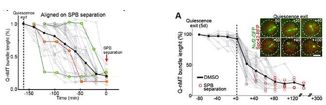
We can add this piece of data in a Sup Figure if the Reviewer believes it is important.
Reviewer #2 (Recommendations For The Authors):
General:
In general, more precise language that accurately describes the experiments would improve the text. <br /> We have tried to do our best to improve the text.
The authors should clearly define what they mean by an active process and provide context to support this statement regarding the Q-nMT.
We have strived to clarify this point in the text (see paragraph form line 146 to 178).
- It is reasonable to assume that structures composed of microtubules are dynamic during the assembly process. The authors should clarify what they mean by "stable by default i.e., intrinsically stable." Do they mean that when Q-nMT assembly starts, it will proceed to completion regardless of a change in condition?
We mean that in phase I the Q-nMT bundle is stabilized as it grows and that stabilization is concomitant with polymerization. By contrast, MTs polymerized during phase II are not stabilized upon elongation beyond the phase I polymer, and get stabilized later, in a separate phase (i.e. in phase III). We hope to have clarified this point in the text (see line 108-110).
- In lines 33-34, the authors claim that the Q-nMT bundle functions as a "sort of checkpoint for cell cycle resumption." This wording is imprecise, and more significantly the authors do not provide evidence supporting a direct role for Q-nMT in a quiescence checkpoint that inhibits re-entry into the cell cycle.
We have softened and clarified the text in the abstract (see line 29-30)., in the introduction (line 101104), in the result section (line 331-332) and in the discussion (line 426-430).
- Many statements are qualitative and subjective. Quantitative statements supported by the results should be used where possible, and if not possible restated or removed.
We provide statistical data analysis for all the figures.
- The number of hours after glucose exhaustion used for each phase varies between assays. This is likely a logistical issue but should be explained.
This is indeed a logistical issue and when pertinent, it is explained in the text.
- It would be interesting to address how this process occurs in diploids. Do they form a Q-nMT? How does this relate to the decision to enter meiosis?
Diploid cells enter meiosis when they are starved for nitrogen. Upon glucose exhaustion diploids do form a Q-nMT bundle. This is shown and measured in the new Sup Fig1C. In fact, in diploids, Q-nMT bundles are thicker than in haploid cells.
- It would be interesting to address how the timescale of this process compares to the types of nutrient stress yeast would be exposed to in the environment.
We have transferred proliferating yeast cells to water, to try to mimic what could happen when yeast cells face rain in the wild. As shown below, they do form a Q-nMT bundle that becomes nocodazole resistant after 30h. This data is now provided in the new Sup Fig 1D.
- It is recommended that the authors use FRAP experiments to directly measure the stability of the QnMT bundles.
This experiment was published in (Laporte et al, 2013). Please see response to Reviewer #1.
- In many cases, the description of the experimental methods lacks sufficient detail to evaluate the approach or for independent verification of results.
We have strived to provide a more detailed material and methods section, as well as more detailed figure legends and statistical informations.
Specific comments on figures:
- In Figure 1 c), what do the polygons represent? They do not contain all the points of the associated colour.
The polygon represented the area of distribution of 90% of the data points. As they did not significantly add to the data presentation they have been removed.
- In Figure 2 a), is the use of two different sets of markers to control for the effect of the markers on microtubule dynamics?
Yes, we are always concerned about the influence of GFP on our results, so very often we replicate our experiments with different fluorescent proteins or even with different proteins tagged with GFP. This is now mentioned in the text (line 184-186).
- Is it accurate to say (line 201, figure 3 a)) that no Q-nMT bundles were detected in ndc80-1 cells shifted to 37 degrees, or are they just shorter?
As shown in Fig 3A, in ndc80-1 cells, most of the MT structures that we measured are below 0,5um. This has been re-phrased in the text (line 214-215).
- Lines 265-269, figure 4 b), how can the phenotype observed in cin8∆ cells be explained given the low abundance of Cin8 that is detected in quiescent cells?
Faint fluorescence signal is not synonymous of an absence of function. As shown in Sup Fig 4B, we do detect Cin8-GFP in quiescent cells.
- Quantification is needed in Figure 4 panels c) and h).
Fig 4C and 4H have been changed and quantification are provided in the figure legend.
Reviewer #3 (Recommendations For The Authors):
A few points should be addressed for clarity:
(1) Sup. Fig. 1K: are only viable cells used for the colony-forming assay? How were these selected? If not, the assay would just measure survival (as in the viability assay).
Yes, only viable cells were selected for the colony forming assay. We used methylene blue to stain dead cells. Then, we used a micromanipulation instrument (Singer Spore Play) that is commonly used for tetrad dissection to select “non blue cells” and position them on a plate (as we do with spores). Each micromanipulated cell is then allowed to grow on the plate and we count colonies (see picture in Sup Fig 1L right panel). This was described in Laporte et al, JCB 2011. We have added that piece of information in the legend (line 1129-1130) and in the M&M section (line 580-586).
(2) Could Tub3 have a role in phase I? It is not clear why the authors conclude involvement only in phase II.
As it can be seen in Fig 2D, MT bundle length and thickness are quite similar in WT and Tub1-only cells in phase I, indicating that the absence of Tub3 as no effect in phase I. In Tub1-only cells, MT bundles are thinner in both phase II and phase III, yet, they get fully stabilized in phase III. Thus, the effect of Tub3 is largely specific to the nucleation/elongation of phase II MTs. We hope to have clarified that point in the text (line 203-207).
(3) Quantifications, statistics: for all quantifications, the authors should clearly state the number of experiments (replicates), and number of cells used in each, and what number was used for statistics. For all quantifications in cells, it seems that the values from the total number of cells across different experiments were plotted and used for statistics. This is not very useful and results in extremely small p values. I assume that the values for individual cells were obtained from multiple, independent experiments. Unless there are technical limitations that allow only a very small sample size (not the case here for most experiments), for experiments involving treatments the authors should determine values for each experiment and show statistics for comparison between experiments rather than individual cells pooled from multiple experiments.
All the experiments have been done at least in replicate. In the new Fig. 1A, we now display each independent experiment with a specific color code. For Fig 2B and 2C we now provide the data obtained for each separate experiment in Sup Fig 2C. Additional details about quantifications and statistics are provided in the M&M section or in the specific figure legends.
Author response:
The following is the authors’ response to the previous reviews.
Reviewer #1:
I am satisfied with all clarifications and additional analyses performed by the authors.
The only concern I have is about changes in running after [AM+VM] mismatches.
The authors reported that they "found no evidence of a change in running speed or pupil diameter following [AM + VM] mismatch (Figures S5A)" (line 197).
Nevertheless, it seems that there is a clear increase in running speed for the [AM+VM] condition (S5A). Could this be more specifically quantified? I am concerned that part of the [AM+VM] could stem from this change in running behavior. Could one factor out the running contribution?
Please excuse, this was unintentionally omitted. We have added the quantification to Table S1 and included the results of the significance test in (Fig S2A, Fig S4A and Fig S5A). The increase in running speed upon MM presentation (0.5 – 1 s), compared to the baseline running speed in the time window preceding MM presentation (-0.5 – 0 s), was not significant in any of the tested conditions.
In the process of adding the statistics, we noticed an unfortunate inconsistency in our figures that relates to Figure S5A. The data shown in all other Figures is aligned to the onset of audiomotor mismatch. In Figure S5A, however, the data were aligned to the onset of the visuomotor mismatch. As there is a differential delay in the closed loop coupling of auditory and visual feedback of approximately 170 ms (as described in the methods), visuomotor mismatch onset is slightly before audiomotor mismatch onset. We have corrected this now in the manuscript but have done the statistical analysis for both old and new versions of the figure. In neither case do we find evidence of a running speed response.
The authors thoroughly addressed the concerns raised. In my opinion, this has substantially strengthened the manuscript, enabling much clearer interpretation of the results reported. I commend the authors for the response to review. Overall, I find the experiments elegantly designed, and the results robust, providing compelling evidence for non-hierarchical interactions across neocortical areas and more specifically for the exchange of sensorimotor prediction error signals across modalities.
We are happy to hear!
Reviewer #2:
The incorporation of the analysis of the animal's running speed and the pupil size upon sound interruption improves the interpretation of the data. The authors can now conclude that responses to the mismatch are not due to behavioral effects.
The issue of the relationship between mismatch responses and offset responses remains uncommented. The auditory system is sensitive to transitions, also to silence. See the work of the Linden or the Barkat labs (including the work of the first author of this manuscript) on offset responses, and also that of the Mesgarani lab (Khalighinejad et al., 2019) on responses to transitions 'to clean' (Figure 1c) in human auditory cortex. Offset responses, as the first author knows well, are modulated by intensity and stimulus length (after adaptation?). That responses to the interruption of the sound are similar in quality, if not quantity, in the closed and open loop conditions suggest that offset response might modulate the mismatch response. A mismatch response that reflects a break in predictability would presumably be less modulated by the exact details of the sensory input than an offset response. Therefore, what is the relationship between the mismatch response and the mean sound amplitude prior to the sound interruption (for example during the preceding 1 second)? And between the mismatch response and the mean firing rate over the same period?
Finally, how do visual stimuli modulate sound responses in the absence of a mismatch? Is the multimodal response potentiation specific to a mismatch?
There are probably two points important to clarify before answering the question – just to make sure there is no semantic misunderstanding.
(1) In the jargon of predictive processing, a prediction error is a deviation from a predictable relationship. This can be sensorimotor coupling (as in audio- and visuomotor mismatch), stimulus history (as in oddball, or sound offset responses), surround sensory input (as in endstopping response and center-surround effects in visual processing), etc. A sound offset perceived by an animal in an open loop condition is thus a negative prediction error based on stimulus history (this assumes the animal has no way to predict the time of offset – as is the case in our experiments). We are primarily interested in our work here in characterizing negative prediction errors that result from motor-related predictions – hence the comparison we use is unpredictable sound offset in closed-loop coupling vs. unpredictable sound offset in open-loop coupling. The first is a mixture of an audiomotor prediction error and a stimulus history prediction error. The second is just a stimulus history prediction error. Thus, we compare the two types of responses to isolate the component that can only be attributed to audiomotor prediction errors.
(2) Audiomotor mismatch responses can of course be explained in a large variety of ways. For example, one could consider a sound offset a sensory stimulus. One could further assume that locomotion increases sensory responses. If so, one could explain audiomotor mismatch responses as a locomotion related gain of a sensory offset response. However, we need to further postulate that this locomotion related gain is stimulus specific, as for sound onset responses there is no detectable difference between locomotion and sitting. Thus, we are left with a model that explains audiomotor mismatch responses as a “stimulus specific locomotion gain of sensory responses”. This is correct – it is just not very satisfying, has no computational basis, and makes no useful predictions (see e.g. https://pubmed.ncbi.nlm.nih.gov/36821437/ for an extended treatise of exactly this point for visuomotor mismatch responses).
That responses to the interruption of the sound are similar in quality, if not quantity, in the closed and open loop conditions suggest that offset response might modulate the mismatch response.
Conceptually both a “sound offset” and an “audiomotor mismatch” are negative prediction errors. Could one describe the effect we see as an audiomotor mismatch modulating a sound offset? Certainly. But if the reviewer means modulate in the sense of neuromodulatory – we are not aware of a neuromodulatory responses that would be fast enough (or be strong enough to have these effects – we have looked into ACh, NA, and Ser (unpublished – no MM response)). Alternatively, they could simply add linearly (as predictive processing would predict). Given that AM mismatch responses are likely computed in auditory cortex, we see no reason to speculate that anything more complicated is happening than a linear summation of different prediction error responses.
A mismatch response that reflects a break in predictability would presumably be less modulated by the exact details of the sensory input than an offset response. Therefore, what is the relationship between the mismatch response and the mean sound amplitude prior to the sound interruption (for example during the preceding 1 second)? And between the mismatch response and the mean firing rate over the same period?
The reviewer’s intuition here – that mismatch responses have a lower resolution than what one thinks of as sensory responses (or sound offset responses) – is probably not warranted. Experiments that quantify the resolution of mismatch responses are relatively data intense – and to the best of our knowledge this has only been done once in the visual system for visuomotor mismatch responses (Zmarz and Keller, 2016). Here we found that visuomotor mismatch responses exhibited matched spatial (in visual space) resolution to that of visual responses.
Regarding the suggested analyses: In a closed loop session, the sound amplitude preceding the mismatch is directly related to the running speed of the mouse. In visual cortex, the amplitude of visuomotor mismatch responses linearly scales with running speed (and consequently visual flow speed) prior to the mismatch – as predicted by predictive processing. See e.g. figure 4B in (Zmarz and Keller, 2016). We have tried this analysis for audiomotor mismatches in the previous round of reviews, but we fear we do not have sufficient data to address this question properly. If we look at how mismatch responses change as a function of locomotion speed (sound amplitude) across the entire population of neurons, we have no evidence of a systematic change (and the effects are highly variable as a function of speed bins we choose). However, just looking at the most audiomotor mismatch responsive neurons, we find a trend for increased responses with increasing running speed (Author response image 1). We analyzed the top 5% of cells that showed the strongest response to mismatch (MM) and divided the MM trials into three groups based on running speed: slow (10-20 cm/s), middle (20-30 cm/s), and fast (>30 cm/s). Given the fact that we have on average 14 mismatch events in total per neuron, the analysis when split by running speed is under-powered.
Author response image 1.
The average response of strongest AM MM responders to AM mismatches as a function of running speed (data are from 51 cells, 11 fields of view, 6 mice).
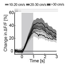
Regarding the relationship between mismatch response and firing rate prior to mismatch, we are not sure we understand the intuition. Does the reviewer mean, the average firing rate of the mismatch neuron? Or the population mean? The first is likely uninterpretable as it is bound to be confounded by regression to the mean type artefacts. But in either case, we would have no prediction of what to expect.
Author response:
The following is the authors’ response to the previous reviews
Reviewer #1:
Comment:
The authors quantified information in gesture and speech, and investigated the neural processing of speech and gestures in pMTG and LIFG, depending on their informational content, in 8 different time-windows, and using three different methods (EEG, HD-tDCS and TMS). They found that there is a time-sensitive and staged progression of neural engagement that is correlated with the informational content of the signal (speech/gesture).
Strengths:
A strength of the paper is that the authors attempted to combine three different methods to investigate speech-gesture processing.
We sincerely appreciate the reviewer’s recognition of our efforts in employing a multi-method approach, which integrates three complementary experimental paradigms, each leveraging distinct neurophysiological techniques to provide converging evidence.
In Experiment 1, we found that the degree of inhibition in the pMTG and LIFG was strongly associated with the overlap in gesture-speech representations, as quantified by mutual information. Experiment 2 revealed the time-sensitive dynamics of the pMTG-LIFG circuit in processing both unisensory (gesture or speech) and multisensory information. Experiment 3, utilizing high-temporal-resolution EEG, independently replicated the temporal dynamics of gesture-speech integration observed in Experiment 2, further validating our findings.
The striking convergence across these methodologically independent approaches significantly bolsters the robustness and generalizability of our conclusions regarding the neural mechanisms underlying multisensory integration.
Comment 1: I thank the authors for their careful responses to my comments. However, I remain not convinced by their argumentation regarding the specificity of their spatial targeting and the time-windows that they used.
The authors write that since they included a sham TMS condition, that the TMS selectively disrupted the IFG-pMTG interaction during specific time windows of the task related to gesture-speech semantic congruency. This to me does not show anything about the specificity of the time-windows itself, nor the selectivity of targeting in the TMS condition.
(1) Selection of brain regions (IFG/pMTG)
We thank the reviewer for their thoughtful consideration. The choice of the left IFG and pMTG as regions of interest (ROIs) was informed by a meta-analysis of fMRI studies on gesture-speech integration, which consistently identified these regions as critical hubs (see Author response table 1 for detailed studies and coordinates).
Author response table 1.
Meta-analysis of previous studies on gesture-speech integration.
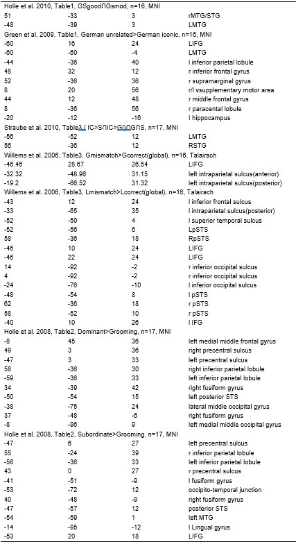
Based on the meta-analysis of previous studies, we selected the IFG and pMTG as ROIs for gesture-speech integration. The rationale for selecting these brain regions is outlined in the introduction in Lines 63-66: “Empirical studies have investigated the semantic integration between gesture and speech by manipulating their semantic relationship[15-18] and revealed a mutual interaction between them19-21 as reflected by the N400 latency and amplitude14 as well as common neural underpinnings in the left inferior frontal gyrus (IFG) and posterior middle temporal gyrus (pMTG)[15,22,23].”
And further described in Lines 77-78: “Experiment 1 employed high-definition transcranial direct current stimulation (HD-tDCS) to administer Anodal, Cathodal and Sham stimulation to either the IFG or the pMTG”. And Lines 85-88: ‘Given the differential involvement of the IFG and pMTG in gesture-speech integration, shaped by top-down gesture predictions and bottom-up speech processing [23], Experiment 2 was designed to assess whether the activity of these regions was associated with relevant informational matrices”.
In the Methods section, we clarified the selection of coordinates in Lines 194-200: “Building on a meta-analysis of prior fMRI studies examining gesture-speech integration[22], we targeted Montreal Neurological Institute (MNI) coordinates for the left IFG at (-62, 16, 22) and the pMTG at (-50, -56, 10). In the stimulation protocol for HD-tDCS, the IFG was targeted using electrode F7 as the optimal cortical projection site[36], with four return electrodes placed at AF7, FC5, F9, and FT9. For the pMTG, TP7 was selected as the cortical projection site[36], with return electrodes positioned at C5, P5, T9, and P9.”
The selection of IFG or pMTG as integration hubs for gesture and speech has also been validated in our previous studies. Specifically, Zhao et al. (2018, J. Neurosci) applied TMS to both areas. Results demonstrated that disrupting neural activity in the IFG or pMTG via TMS selectively impaired the semantic congruency effect (reaction time costs due to semantic incongruence), while leaving the gender congruency effect unaffected.
These findings identified the IFG and pMTG as crucial hubs for gesture-speech integration, guiding the selection of brain regions for our subsequent studies.
(2) Selection of time windows
The five key time windows (TWs) analyzed in this study were derived from our previous TMS work (Zhao et al., 2021, J. Neurosci), where we segmented the gesture-speech integration period (0–320 ms post-speech onset) into eight 40-ms windows. This interval aligns with established literature on gesture-speech integration, particularly the 200–300 ms window noted by the reviewer. As detailed in Lines (776-779): “Procedure of Experiment 2. Eight time windows (TWs, duration = 40 ms) were segmented in relative to the speech IP. Among the eight TWs, five (TW1, TW2, TW3, TW6, and TW7) were chosen based on the significant results in our prior study[23]. Double-pulse TMS was delivered over each of the TW of either the pMTG or the IFG”.
In our prior work (Zhao et al., 2021, J. Neurosci), we employed a carefully controlled experimental design incorporating two key factors: (1) gesture-speech semantic congruency (serving as our primary measure of integration) and (2) gesture-speech gender congruency (implemented as a matched control factor). Using a time-locked, double-pulse TMS protocol, we systematically targeted each of the eight predefined time windows (TWs) within the left IFG, left pMTG, or vertex (serving as a sham control condition). Our results demonstrated that a TW-selective disruption of gesture-speech integration, indexed by the semantic congruency effect (i.e., a cost of reaction time because of semantic conflict), when stimulating the left pMTG in TW1, TW2, and TW7 but when stimulating the left IFG in TW3 and TW6. Crucially, no significant effects were observed during either sham stimulation or the controlled gender congruency factor (Figure 3 from Zhao et al., 2021, J. Neurosci).
This triple dissociation - showing effects only for semantic integration, only in active stimulation, and only at specific time points - provides compelling causal evidence that IFG-pMTG connectivity plays a temporally precise role in gesture-speech integration.
Noted that this work has undergone rigorous peer review by two independent experts who both endorsed our methodological approach. Their original evaluations, provided below:
Reviewer 1: “significance: Using chronometric TMS-stimulation the data of this experiment suggests a feedforward information flow from left pMTG to left IFG followed by an information flow from left IFG back to the left pMTG. The study is the first to provide causal evidence for the temporal dynamics of the left pMTG and left IFG found during gesture-speech integration.”
Reviewer 2: “Beyond the new results the manuscript provides regarding the chronometrical interaction of the left inferior frontal gyrus and middle temporal gyrus in gesture-speech interaction, the study more basically shows the possibility of unfolding temporal stages of cognitive processing within domain-specific cortical networks using short-time interval double-pulse TMS. Although this method also has its limitations, a careful study planning as shown here and an appropiate discussion of the results can provide unique insights into cognitive processing.”
References:
Willems, R.M., Ozyurek, A., and Hagoort, P. (2009). Differential roles for left inferior frontal and superior temporal cortex in multimodal integration of action and language. Neuroimage 47, 1992-2004. 10.1016/j.neuroimage.2009.05.066.
Drijvers, L., Jensen, O., and Spaak, E. (2021). Rapid invisible frequency tagging reveals nonlinear integration of auditory and visual information. Human Brain Mapping 42, 1138-1152. 10.1002/hbm.25282.
Drijvers, L., and Ozyurek, A. (2018). Native language status of the listener modulates the neural integration of speech and iconic gestures in clear and adverse listening conditions. Brain and Language 177, 7-17. 10.1016/j.bandl.2018.01.003.
Drijvers, L., van der Plas, M., Ozyurek, A., and Jensen, O. (2019). Native and non-native listeners show similar yet distinct oscillatory dynamics when using gestures to access speech in noise. Neuroimage 194, 55-67. 10.1016/j.neuroimage.2019.03.032.
Holle, H., and Gunter, T.C. (2007). The role of iconic gestures in speech disambiguation: ERP evidence. J Cognitive Neurosci 19, 1175-1192. 10.1162/jocn.2007.19.7.1175.
Kita, S., and Ozyurek, A. (2003). What does cross-linguistic variation in semantic coordination of speech and gesture reveal?: Evidence for an interface representation of spatial thinking and speaking. J Mem Lang 48, 16-32. 10.1016/S0749-596x(02)00505-3.
Bernardis, P., and Gentilucci, M. (2006). Speech and gesture share the same communication system. Neuropsychologia 44, 178-190. 10.1016/j.neuropsychologia.2005.05.007.
Zhao, W.Y., Riggs, K., Schindler, I., and Holle, H. (2018). Transcranial magnetic stimulation over left inferior frontal and posterior temporal cortex disrupts gesture-speech integration. Journal of Neuroscience 38, 1891-1900. 10.1523/Jneurosci.1748-17.2017.
Zhao, W., Li, Y., and Du, Y. (2021). TMS reveals dynamic interaction between inferior frontal gyrus and posterior middle temporal gyrus in gesture-speech semantic integration. The Journal of Neuroscience, 10356-10364. 10.1523/jneurosci.1355-21.2021.
Hartwigsen, G., Bzdok, D., Klein, M., Wawrzyniak, M., Stockert, A., Wrede, K., Classen, J., and Saur, D. (2017). Rapid short-term reorganization in the language network. Elife 6. 10.7554/eLife.25964.
Jackson, R.L., Hoffman, P., Pobric, G., and Ralph, M.A.L. (2016). The semantic network at work and rest: Differential connectivity of anterior temporal lobe subregions. Journal of Neuroscience 36, 1490-1501. 10.1523/JNEUROSCI.2999-15.2016.
Humphreys, G. F., Lambon Ralph, M. A., & Simons, J. S. (2021). A Unifying Account of Angular Gyrus Contributions to Episodic and Semantic Cognition. Trends in neurosciences, 44(6), 452–463. https://doi.org/10.1016/j.tins.2021.01.006
Bonner, M. F., & Price, A. R. (2013). Where is the anterior temporal lobe and what does it do?. The Journal of neuroscience : the official journal of the Society for Neuroscience, 33(10), 4213–4215. https://doi.org/10.1523/JNEUROSCI.0041-13.2013
Comment 2: It could still equally well be the case that other regions or networks relevant for gesture-speech integration are targeted, and it can still be the case that these timewindows are not specific, and effects bleed into other time periods. There seems to be no experimental evidence here that this is not the case.
The selection of IFG and pMTG as regions of interest was rigorously justified through multiple lines of evidence. First, a comprehensive meta-analysis of fMRI studies on gesture-speech integration consistently identified these regions as central nodes (see response to comment 1). Second, our own previous work (Zhao et al., 2018, JN; 2021, JN) provided direct empirical validation of their involvement. Third, by employing the same experimental paradigm, we minimized the likelihood of engaging alternative networks. Fourth, even if other regions connected to IFG or pMTG might be affected by TMS, the distinct engagement of specific time windows of IFG and pMTG minimizes the likelihood of consistent influence from other regions.
Regarding temporal specificity, our 2021 study (Zhao et al., 2021, JN, see details in response to comment 1) systematically examined the entire 0-320ms integration window and found that only select time windows showed significant effects for gesture-speech semantic congruency, while remaining unaffected during gender congruency processing. This double dissociation (significant effects for semantic integration but not gender processing in specific windows) rules out broad temporal spillover.
Comment 3: To be more specific, the authors write that double-pulse TMS has been widely used in previous studies (as found in their table). However, the studies cited in the table do not necessarily demonstrate the level of spatial and temporal specificity required to disentangle the contributions of tightly-coupled brain regions like the IFG and pMTG during the speech-gesture integration process. pMTG and IFG are located in very close proximity, and are known to be functionally and structurally interconnected, something that is not necessarily the case for the relatively large and/or anatomically distinct areas that the authors mention in their table.
Our methodological approach is strongly supported by an established body of research employing double-pulse TMS (dpTMS) to investigate neural dynamics across both primary motor and higher-order cognitive regions. As documented in Author response table 1, multiple studies have successfully applied this technique to: (1) primary motor areas (tongue and lip representations in M1), and (2) semantic processing regions (including pMTG, PFC, and ATL). Particularly relevant precedents include:
(1) Teige et al. (2018, Cortex): Demonstrated precise spatial and temporal specificity by applying 40ms-interval dpTMS to ATL, pMTG, and mid-MTG across multiple time windows (0-40ms, 125-165ms, 250-290ms, 450-490ms), revealing distinct functional contributions from ATL versus pMTG.
(2) Vernet et al. (2015, Cortex): Successfully dissociated functional contributions of right IPS and DLPFC using 40ms-interval dpTMS, despite their anatomical proximity and functional connectivity.
These studies confirm double-pulse TMS can discriminate interconnected nodes at short timescales. Our 2021 study further validated this for IFG-pMTG.
Author response table 2.
Double-pulse TMS studies on brain regions over 3-60 ms time interval
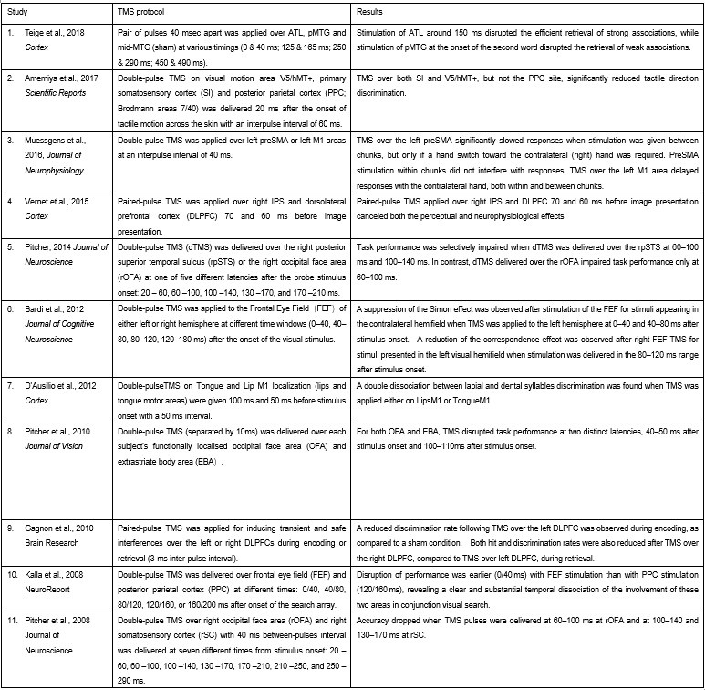
References:
Teige, C., Mollo, G., Millman, R., Savill, N., Smallwood, J., Cornelissen, P. L., & Jefferies, E. (2018). Dynamic semantic cognition: Characterising coherent and controlled conceptual retrieval through time using magnetoencephalography and chronometric transcranial magnetic stimulation. Cortex, 103, 329-349.
Vernet, M., Brem, A. K., Farzan, F., & Pascual-Leone, A. (2015). Synchronous and opposite roles of the parietal and prefrontal cortices in bistable perception: a double-coil TMS–EEG study. Cortex, 64, 78-88.
Comment 4: But also more in general: The mere fact that these methods have been used in other contexts does not necessarily mean they are appropriate or sufficient for investigating the current research question. Likewise, the cognitive processes involved in these studies are quite different from the complex, multimodal integration of gesture and speech. The authors have not provided a strong theoretical justification for why the temporal dynamics observed in these previous studies should generalize to the specific mechanisms of gesture-speech integration..
The neurophysiological mechanisms underlying double-pulse TMS (dpTMS) are well-characterized. While it is established that single-pulse TMS can produce brief artifacts (typically within 0–10 ms) due to transient cortical depolarization (Romero et al., 2019, NC), the dynamics of double-pulse TMS (dpTMS) involve more intricate inhibitory interactions. Specifically, the first pulse increases membrane conductance via GABAergic shunting inhibition, effectively lowering membrane resistance and attenuating the excitatory impact of the second pulse. This results in a measurable reduction in cortical excitability at the paired-pulse interval, as evidenced by suppressed motor evoked potentials (MEPs) (Paulus & Rothwell, 2016, J Physiol). Importantly, this neurophysiological mechanism is independent of cognitive domain and has been robustly demonstrated across multiple functional paradigms.
In our study, we did not rely on previously reported timing parameters but instead employed a dpTMS protocol using a 40-ms inter-pulse interval. Based on the inhibitory dynamics of this protocol, we designed a sliding temporal window sufficiently broad to encompass the integration period of interest. This approach enabled us to capture and localize the critical temporal window associated with ongoing integrative processing in the targeted brain region.
We acknowledge that the previous phrasing may have been ambiguous, a clearer and more detailed description of the dpTMS protocol has now been provided in Lines 88-92: “To this end, we employed chronometric double-pulse transcranial magnetic stimulation, which is known to transiently reduce cortical excitability at the inter-pulse interval]27]. Within a temporal period broad enough to capture the full duration of gesture–speech integration[28], we targeted specific timepoints previously implicated in integrative processing within IFG and pMTG [23].”
References:
Romero, M.C., Davare, M., Armendariz, M. et al. Neural effects of transcranial magnetic stimulation at the single-cell level. Nat Commun 10, 2642 (2019). https://doi.org/10.1038/s41467-019-10638-7
Paulus W, Rothwell JC. Membrane resistance and shunting inhibition: where biophysics meets state-dependent human neurophysiology. J Physiol. 2016 May 15;594(10):2719-28. doi: 10.1113/JP271452. PMID: 26940751; PMCID: PMC4865581.
Obermeier, C., & Gunter, T. C. (2015). Multisensory Integration: The Case of a Time Window of Gesture-Speech Integration. Journal of Cognitive Neuroscience, 27(2), 292-307. https://doi.org/10.1162/jocn_a_00688
Comment 5: Moreover, the studies cited in the table provided by the authors have used a wide range of interpulse intervals, from 20 ms to 100 ms, suggesting that the temporal precision required to capture the dynamics of gesture-speech integration (which is believed to occur within 200-300 ms; Obermeier & Gunter, 2015) may not even be achievable with their 40 ms time windows.
Double-pulse TMS has been empirically validated across neurocognitive studies as an effective method for establishing causal temporal relationships in cortical networks, with demonstrated sensitivity at timescales spanning 3-60 m. Our selection of a 40-ms interpulse interval represents an optimal compromise between temporal precision and physiological feasibility, as evidenced by its successful application in dissociating functional contributions of interconnected regions including ATL/pMTG (Teige et al., 2018) and IPS/DLPFC (Vernet et al., 2015). This methodological approach combines established experimental rigor with demonstrated empirical validity for investigating the precisely timed IFG-pMTG dynamics underlying gesture-speech integration, as shown in our current findings and prior work (Zhao et al., 2021).
Our experimental design comprehensively sampled the 0-320 ms post-stimulus period, fully encompassing the critical 200-300 ms window associated with gesture-speech integration, as raised by the reviewer. Notably, our results revealed temporally distinct causal dynamics within this period: the significantly reduced semantic congruency effect emerged at IFG at 200-240ms, followed by feedback projections from IFG to pMTG at 240-280ms. This precisely timed interaction provides direct neurophysiological evidence for the proposed architecture of gesture-speech integration, demonstrating how these interconnected regions sequentially contribute to multisensory semantic integration.
Comment 6: I do appreciate the extra analyses that the authors mention. However, my 5th comment is still unanswered: why not use entropy scores as a continous measure?
Analysis with MI and entropy as continuous variables were conducted employing Representational Similarity Analysis (RSA) (Popal et.al, 2019). This analysis aimed to build a model to predict neural responses based on these feature metrics.
To capture dynamic temporal features indicative of different stages of multisensory integration, we segmented the EEG data into overlapping time windows (40 ms in duration with a 10 ms step size). The 40 ms window was chosen based on the TMS protocol used in Experiment 2, which also employed a 40 ms time window. The 10 ms step size (equivalent to 5 time points) was used to detect subtle shifts in neural responses that might not be captured by larger time windows, allowing for a more granular analysis of the temporal dynamics of neural activity.
Following segmentation, the EEG data were reshaped into a four-dimensional matrix (42 channels × 20 time points × 97 time windows × 20 features). To construct a neural similarity matrix, we averaged the EEG data across time points within each channel and each time window. The resulting matrix was then processed using the pdist function to compute pairwise distances between adjacent data points. This allowed us to calculate correlations between the neural matrix and three feature similarity matrices, which were constructed in a similar manner. These three matrices corresponded to (1) gesture entropy, (2) speech entropy, and (3) mutual information (MI). This approach enabled us to quantify how well the neural responses corresponded to the semantic dimensions of gesture and speech stimuli at each time window.
To determine the significance of the correlations between neural activity and feature matrices, we conducted 1000 permutation tests. In this procedure, we randomized the data or feature matrices and recalculated the correlations repeatedly, generating a null distribution against which the observed correlation values were compared. Statistical significance was determined if the observed correlation exceeded the null distribution threshold (p < 0.05). This permutation approach helps mitigate the risk of spurious correlations, ensuring that the relationships between the neural data and feature matrices are both robust and meaningful.
Finally, significant correlations were subjected to clustering analysis, which grouped similar neural response patterns across time windows and channels. This clustering allowed us to identify temporal and spatial patterns in the neural data that consistently aligned with the semantic features of gesture and speech stimuli, thus revealing the dynamic integration of these multisensory modalities across time. Results are as follows:
(1) Two significant clusters were identified for gesture entropy (Figure 1 left). The first cluster was observed between 60-110 ms (channels F1 and F3), with correlation coefficients (r) ranging from 0.207 to 0.236 (p < 0.001). The second cluster was found between 210-280 ms (channel O1), with r-values ranging from 0.244 to 0.313 (p < 0.001).
(2) For speech entropy (Figure 1 middle), significant clusters were detected in both early and late time windows. In the early time windows, the largest significant cluster was found between 10-170 ms (channels F2, F4, F6, FC2, FC4, FC6, C4, C6, CP4, and CP6), with r-values ranging from 0.151 to 0.340 (p = 0.013), corresponding to the P1 component (0-100 ms). In the late time windows, the largest significant cluster was observed between 560-920 ms (across the whole brain, all channels), with r-values ranging from 0.152 to 0.619 (p = 0.013).
(3) For mutual information (MI) (Figure 1 right), a significant cluster was found between 270-380 ms (channels FC1, FC2, FC3, FC5, C1, C2, C3, C5, CP1, CP2, CP3, CP5, FCz, Cz, and CPz), with r-values ranging from 0.198 to 0.372 (p = 0.001).
Author response image 1.
Results of RSA analysis.
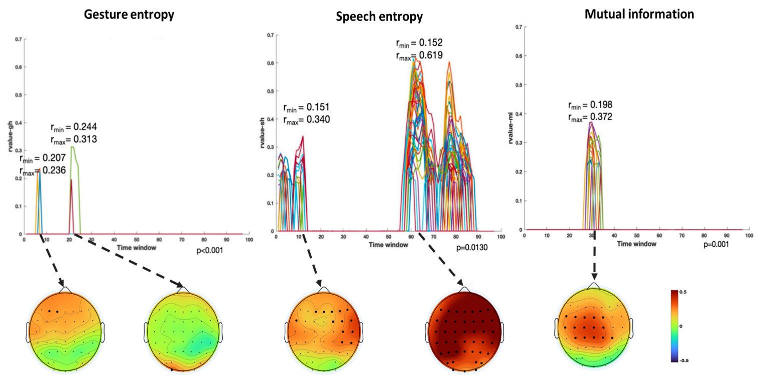
These additional findings suggest that even using a different modeling approach, neural responses, as indexed by feature metrics of entropy and mutual information, are temporally aligned with distinct ERP components and ERP clusters, as reported in the current manuscript. This alignment serves to further consolidate the results, reinforcing the conclusion we draw. Considering the length of the manuscript, we did not include these results in the current manuscript.
Reference:
Popal, H., Wang, Y., & Olson, I. R. (2019). A guide to representational similarity analysis for social neuroscience. Social cognitive and affective neuroscience, 14(11), 1243-1253.
Comment 7: In light of these concerns, I do not believe the authors have adequately demonstrated the spatial and temporal specificity required to disentangle the contributions of the IFG and pMTG during the gesture-speech integration process. While the authors have made a sincere effort to address the concerns raised by the reviewers, and have done so with a lot of new analyses, I remain doubtful that the current methodological approach is sufficient to draw conclusions about the causal roles of the IFG and pMTG in gesture-speech integration.
To sum up:
(1) Empirical validation from our prior work (Zhao et al., 2018,2021,JN): The selection of IFG and pMTG as target regions was informed by both: (1) a comprehensive meta-analysis of fMRI studies on gesture-speech integration, and (2) our own prior causal evidence from Zhao et al. (2018, J Neurosci), with detailed stereotactic coordinates provided in the attached Response to Editors and Reviewers letter. The temporal parameters were similarly grounded in empirical data from Zhao et al. (2021, J Neurosci), where we systematically examined eight consecutive 40-ms windows spanning the full integration period (0-320 ms). This study revealed a triple dissociation of effects - occurring exclusively during: (i)semantic integration (but not control tasks), (ii) active stimulation (but not sham), and (iii) specific time windows (but not all time windows)- providing robust causal evidence for the spatiotemporal specificity of IFG-pMTG interactions in gesture-speech processing. Notably, all reviewers recognized the methodological strength of this dpTMS approach in their evaluations (see attached JN assessment for details).
(2) Convergent evidence from Experiment 3: Our study employed a multi-method approach incorporating three complementary experimental paradigms, each utilizing distinct neurophysiological techniques to provide converging evidence. Specifically, Experiment 3 implemented high-temporal-resolution EEG, which independently replicated the time-sensitive dynamics of gesture-speech integration observed in our double-pulse TMS experiments. The remarkable convergence between these methodologically independent approaches -demonstrating consistent temporal staging of IFG-pMTG interactions across both causal (TMS) and correlational (EEG) measures - significantly strengthens the validity and generalizability of our conclusions regarding the neural mechanisms underlying multisensory integration.
(3) Established precedents in double-pulse TMS literature: The double-pulse TMS methodology employed in our study is firmly grounded in established neuroscience research. As documented in our detailed Response to Editors and Reviewers letter (citing 11 representative studies), dpTMS has been extensively validated for investigating causal temporal dynamics in cortical networks, with demonstrated sensitivity at timescales ranging from 3-60 ms. Particularly relevant precedents include: 1. Teige et al. (2018, Cortex) successfully dissociated functional contributions of anatomically proximal regions (ATL vs. pMTG vs.mid-MTG) using 40-ms-interval double-pulse TMS; 2. Vernet et al. (2015, Cortex) effectively distinguished neural processing in interconnected frontoparietal regions (right IPS vs. DLPFC) using 40-ms double-pulse TMS parameters. Both parameters are identical to those employed in our current study.
(4) Neurophysiological Plausibility: The neurophysiological basis for the transient double-pulse TMS effects is well-established through mechanistic studies of TMS-induced cortical inhibition (Romero et al.,2019; Paulus & Rothwell, 2016).
Taking together, we respectfully submit that our methodology provides robust support for our conclusions.
Author response:
The following is the authors’ response to the previous reviews.
We thank you for the time you took to review our work and for your feedback!
The major changes to the manuscript are:
(1) We have added visual flow speed and locomotion velocity traces to Figure 5 as suggested.
(2) We have rephrased the abstract to more clearly indicate that our statement regarding acetylcholine enabling faster switching of internal representations in layer 5 is speculative.
(3) We have further clarified the positioning of our findings regarding the basal forebrain cholinergic signal in visual cortex in the introduction.
(4) We have added a video (Video S1) to illustrate different mouse running speeds covered by our data.
A detailed point-by-point response to all reviewer concerns is provided below.
Reviewer #1 (Recommendations For The Authors):
The authors have addressed most of the concerns raised in the initial review. While the paper has been improved, there are still some points of concern in the revised version.
Major comments
(1) Page 1, Line 21: The authors claim, "Our results suggest that acetylcholine augments the responsiveness of layer 5 neurons to inputs from outside of the local network, enabling faster switching between internal representations during locomotion." However, it is not clear which specific data or results support the claim of "switching between internal representations." ...
Authors' response: "... That acetylcholine enables a faster switching between internal representations in layer 5 is a speculation. We have attempted to make this clearer in the discussion. ..."
In the revised version, there is no new data added to directly support the claim - "Our results suggest acetylcholine ..., enabling faster switching between internal representations during locomotion" (in the abstract). The authors themselves acknowledge that this statement is speculative. The present data only demonstrate that ACh reduces the response latency of L5 neurons to visual stimuli, but not that ACh facilitates quicker transitions in neuronal responses from one visual stimulus to another. To maintain scientific rigor and clarity, I recommend the authors amend this sentence to more accurately reflect the findings.
This might be a semantic disagreement? We would argue both a gray screen and a grating are visual stimuli. Hence, we are not sure we understand what the reviewer means by “but not that ACh facilitates quicker transitions in neuronal responses from one visual stimulus to another”. We concur, our data only address one of many possible transitions, but it is a switch between distinct visual stimuli that is sped up by ACh. Nevertheless, we have rephrased the sentence in question by changing “our data suggest” to “based on this we speculate” - but are not sure whether this addresses the reviewer’s concern.
(2) Page 4, Line 103: "..., a direct measurement of the activity of cholinergic projection from basal forebrain to the visual cortex during locomotion has not been made." This statement is incorrect. An earlier study by Reimer et al. indeed imaged cholinergic axons in the visual cortex of mice running on a wheel.
Authors' response: "We have clarified this as suggested. However, we disagree slightly with the reviewer here. The key question is whether the cholinergic axons imaged originate in basal forebrain. While Reimer et al. 2016 did set out to do this, we believe a number of methodological considerations prevent this conclusion: ... Collins et al. 2023 inject more laterally and thus characterize cholinergic input to S1 and A1, ..."
The authors pointed out some methodological caveats in previous studies that measured the BF input in V1, and I agree with them on several points. Nonetheless, the statement that "a direct measurement of the activity of cholinergic projection from basal forebrain to visual cortex during locomotion has not been made. ... Prior measurements of the activity of cholinergic axons in visual cortex have all relied on data from a cross of ChAT-Cre mice with a reporter line ..." (Page 4, Line 103) seems to be an oversimplification. In fact, contrary to what the authors noted, Collins et al. (2023) conducted direct imaging of BF cholinergic axons in V1 (Fig. 1) - "Selected axon segments were chosen from putative retrosplenial, somatosensory, primary and secondary motor, and visual cortices". They used a viral approach to express GCaMP in BF axons to bypass the limitations associated with the use of a GCaMP reporter mouse line - "Viral injections were used for BF- ACh studies to avoid imaging axons or dendrites from cholinergic projections not arising from the BF (e.g. cortical cholinergic interneurons)." The authors should reconsider the text.
The reason we think that our statement here was – while simplified – accurate, is that Collins et al. do record from cholinergic axons in V1, but they don’t show these data (they only show pooled data across all recordings sites). By superimposing the recording locations of the Collins paper on the Allen mouse brain atlas (Figure R1), we estimate that of the approximately 50 recording sites, most are in somatosensory and somatomotor areas of cortex, and only 1 appears to be in V1, something that is often missed as it is not really highlighted in that paper. If this is indeed correct, we would argue that the data in the Collins et al. paper are not representative of cholinergic activity in visual cortex (we fear only the authors would know for sure). Nevertheless, we have rephrased again.
Author response image 1.
Overlay of the Collins et al. imaging sites (red dots, black outline and dashed circle) on the Allen mouse brain atlas (green shading). Very few (we estimate that it was only 1) of the recording sites appear to be in V1 (the lightest green area), and maybe an additional 4 appear to be in secondary visual areas.
Minor comments
(1) It is unclear which BF subregion(s) were targeted in this study.
Authors' response: Thanks for pointing this out. We targeted the entire basal forebrain (medial septum, vertical and horizontal limbs of the diagonal band, and nucleus basalis) with our viral injections. ... We have now added the labels for basal forebrain subregions targeted next to the injection coordinates in the manuscript.
The authors provided the coordinates for their virus injections targeting the BF subregions - "(AP, ML, DV (in mm): ... ; +0.6, +0.6, -4.9 (nucleus basalis) ..." Is this the right coordinates for the nucleus basalis?
Thank you for catching this - this was indeed incorrect. The coordinates were correct, but our annotation of brain region was not (as the reviewer correctly points out, these coordinates are in the horizontal limb of the diagonal band, not the nucleus basalis). We have corrected this.
Reviewer #2 (Recommendations For The Authors):
Thank you for addressing most of the points raised in my original review. I still some concerns relating to the analysis of the data.
(1) I appreciate the authors point that getting mice to reliably during head-fixed recordings can require training. Since mice in this study were not trained to run, their low speed of locomotion limits the interpretation of the results. I think this is an important potential caveat and I have retained it in the public review.
This might be a misunderstanding. The Jordan paper was a bit of an outlier in that we needed mice to run at very high rates due to fact that our recording times was only minutes. Mice were chosen such that they would more or less continuously run, to maximize the likelihood that they would run during the intracellular recordings. This was what we tried to convey in our previous response. The speed range covered by the analysis in this paper is 0 cm/s to 36 cm/s. 36 cm/s is not far away from the top speed mice can reach on this treadmill (30 cm/s is 1 revolution of the treadmill per second). In our data, the top speed we measured across all mice was 36 cm/s. In the Jordan paper, the peak running speed across the entire dataset was 44 cm/s. Based on the reviewer’s comment, we suspect that the reviewer may be under the impression that 30 cm/s is a relatively slow running speed. To illustrate what this looks like we have made added a video (Video S1) to illustrate different running speeds.
(2) The majority of the analyses in the revised manuscript focus on grand average responses, which may mask heterogeneity in the underlying neural populations. This could be addressed by analysing the magnitude and latency of responses for individual neurons. For example, if I understand correctly, the analyses include all neurons, whether or not they are activated, inhibited, or unaffected by visual stimulation and locomotion. For example, while on average layer 2/3 neurons are suppressed by the grating stimulus (Figure 4A), presumable a subset are activated. Evaluating the effects of optogenetic stimulation and locomotion without analyzing them at the level of individual neurons could result in misleading conclusions. This could be presented in the form of a scatter plot, depicting the magnitude of neuronal responses in locomotion vs stationary condition, and opto+ vs no opto conditions.
We might be misunderstanding. The first part of the comment is a bit too unspecific to address directly. In cases in which we find the variability is relevant to our conclusions, we do show this for individual cells (e.g.the latencies to running onset are shown as histograms for all cells and axons in Figure S1). It is also unclear to us what the reviewer means by “Evaluating the effects of optogenetic stimulation and locomotion without analyzing them at the level of individual neurons could result in misleading conclusions”. Our conclusions relate to the average responses in L2/3, consistent with the analysis shown. All data will be freely available for anyone to perform follow-up analysis of things we may have missed. E.g., the specific suggestion of presenting the data shown in Figure 4 as a scatter plot is shown below (Figure R2). This is something we had looked at but found not to be relevant to our conclusions. The problem with this analysis is that it is difficult to estimate how much the different sources of variability contribute to the total variability observed in the data, and no interesting pattern is clearly apparent. All relevant and clear conclusions are already captured by the mean differences shown in Figure 4.
Author response image 2.
Optogenetic activation of cholinergic axons in visual cortex primarily enhances responses of layer 5, but not layer 2/3 neurons. Related to Figure 4. (A) Average calcium response of layer 2/3 neurons in visual cortex to full field drifting grating in the absence or presence of locomotion. Each dot is the average calcium activity of an individual neuron during the two conditions. (B) As in A, but for layer 5 neurons. (C) As in A, but comparing the average response while the mice were stationary, to that while cholinergic axons were optogenetically stimulated. (D) As in C, but for layer 5 neurons. (E) Average calcium response of layer 2/3 neurons in visual cortex to visuomotor mismatch, without and with optogenetic stimulation of cholinergic axons in visual cortex. (F) As in E, but for layer 5 neurons. (G) Average calcium response of layer 2/3 neurons in visual cortex to locomotion onset in closed loop, without and with optogenetic stimulation of cholinergic axons in visual cortex. (H) As in G, but for layer 5 neurons.
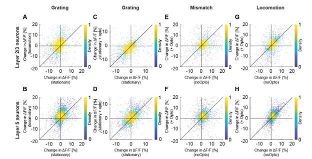
(3) To help the reader understand the experimental conditions in open loop experiments, please include average visual flow speed traces for each condition in Figure 5.
We have added the locomotion velocity and visual flow speeds to the corresponding conditions in Figure
Author response:
The following is the authors’ response to the original reviews.
Public Reviews:
Reviewer #1:
Summary:
The work by Combrisson and colleagues investigates the degree to which reward and punishment learning signals overlap in the human brain using intracranial EEG recordings. The authors used information theory approaches to show that local field potential signals in the anterior insula and the three sub regions of the prefrontal cortex encode both reward and punishment prediction errors, albeit to different degrees. Specifically, the authors found that all four regions have electrodes that can selectively encode either the reward or the punishment prediction errors. Additionally, the authors analyzed the neural dynamics across pairs of brain regions and found that the anterior insula to dorsolateral prefrontal cortex neural interactions were specific for punishment prediction errors whereas the ventromedial prefrontal cortex to lateral orbitofrontal cortex interactions were specific to reward prediction errors. This work contributes to the ongoing efforts in both systems neuroscience and learning theory by demonstrating how two differing behavioral signals can be differentiated to a greater extent by analyzing neural interactions between regions as opposed to studying neural signals within one region.
Strengths:
The experimental paradigm incorporates both a reward and punishment component that enables investigating both types of learning in the same group of subjects allowing direct comparisons.
The use of intracranial EEG signals provides much needed insight into the timing of when reward and punishment prediction errors signals emerge in the studied brain regions.
Information theory methods provide important insight into the interregional dynamics associated with reward and punishment learning and allows the authors to assess that reward versus punishment learning can be better dissociated based on interregional dynamics over local activity alone.
We thank the reviewer for this accurate summary. Please find below our answers to the weaknesses raised by the reviewer.
Weaknesses:
The analysis presented in the manuscript focuses solely on gamma band activity. The presence and potential relevance of other frequency bands is not discussed. It is possible that slow oscillations, which are thought to be important for coordinating neural activity across brain regions could provide additional insight.
We thank the reviewer for pointing us to this missing discussion in the first version of the manuscript. We now made this point clearer in the Methods sections entitled “iEEG data analysis” and “Estimate of single-trial gamma-band activity”:
“Here, we focused solely on broadband gamma for three main reasons. First, it has been shown that the gamma band activity correlates with both spiking activity and the BOLD fMRI signals (Lachaux et al., 2007; Mukamel et al., 2004; Niessing et al., 2005; Nir et al., 2007), and it is commonly used in MEG and iEEG studies to map task-related brain regions (Brovelli et al., 2005; Crone et al., 2006; Vidal et al., 2006; Ball et al., 2008; Jerbi et al., 2009; Darvas et al., 2010; Lachaux et al., 2012; Cheyne and Ferrari, 2013; Ko et al., 2013). Therefore, focusing on the gamma band facilitates linking our results with the fMRI and spiking literatures on probabilistic learning. Second, single-trial and time-resolved high-gamma activity can be exploited for the analysis of cortico-cortical interactions in humans using MEG and iEEG techniques (Brovelli et al., 2015; 2017; Combrisson et al., 2022). Finally, while previous analyses of the current dataset (Gueguen et al., 2021) reported an encoding of PE signals at different frequency bands, the power in lower frequency bands were shown to carry redundant information compared to the gamma band power.”
The data is averaged across all electrodes which could introduce biases if some subjects had many more electrodes than others. Controlling for this variation in electrode number across subjects would ensure that the results are not driven by a small subset of subjects with more electrodes.
We thank the reviewer for raising this important issue. We would like to point out that the gamma activity was not averaged across bipolar recordings within an area, nor measures of connectivity. Instead, we used a statistical approach proposed in a previous paper that combines non-parametric permutations with measures of information (Combrisson et al., 2022). As we explain in the “Statistical analysis” section, mutual information (MI) is estimated between PE signals and single-trial modulations in gamma activity separately for each contact (or for each pair of contacts). Then, a one-sample t-test is computed across all of the recordings of all subjects to form the effect size at the group-level. We will address the point of the electrode number in our answer below.
The potential variation in reward versus punishment learning across subjects is not included in the manuscript. While the time course of reward versus punishment prediction errors is symmetrical at the group level, it is possible that some subjects show faster learning for one versus the other type which can bias the group average. Subject level behavioral data along with subject level electrode numbers would provide more convincing evidence that the observed effects are not arising from these potential confounds.
We thank the reviewer for the two points raised. We performed additional analyses at the single-participant level to address the issues raised by the reviewer. We should note, however, that these results are descriptive and cannot be generalized to account for population-level effects. As suggested by the reviewer, we prepared two new figures. The first supplementary figure summarizes the number of participants that had iEEG contacts per brain region and pair of brain regions (Fig. S1A in the Appendix). It can be seen that the number of participants sampled in different brain regions is relatively constant (left panel) and the number of participants with pairs of contacts across brain regions is relatively homogeneous, ranging from 7 to 11 (right panel). Fig. S1B shows the number of bipolar derivations per subject and per brain region.
Author response image 1.
Single subject anatomical repartition. (A) Number of unique subject per brain region and per pair of brain regions (B) Number of bipolar derivations per subject and per brain region

The second supplementary figure describes the estimated prediction error for rewarding and punishing trials for each subject (Fig. S2). The single-subject error bars represent the 95th percentile confidence interval estimated using a bootstrap approach across the different pairs of stimuli presented during the three to six sessions. As the reviewer anticipated, there are indeed variations across subjects, but we observe that RPE and PPE are relatively symmetrical, even at the subject level, and tend toward zero around trial number 10. These results therefore corroborate the patterns observed at the group-level.
Author response image 2.
Single-subject estimation of predictions errors. Single-subject trial-wise reward PE (RPE - blue) and punishment PE (PPE - red), ± 95% confidence interval.

Finally, to assess the variability of local encoding of prediction errors across participants, we quantified the proportion of subjects having at least one significant bipolar derivation encoding either the RPE or PPE (Fig. S4). As expected, we found various proportions of unique subjects with significant R/PPE encoding per region. The lowest proportion was achieved in the ventromedial prefrontal cortex (vmPFC) and lateral orbitofrontal cortex (lOFC) for encoding PPE and RPE, respectively, with approximately 30% of the subjects having the effect. Conversely, we found highly reproducible encodings in the anterior insula (aINS) and dorsolateral prefrontal cortex (dlPFC) with a maximum of 100% of the 9 subjects having at least one bipolar derivation encoding PPE in the dlPFC.
Author response image 3.
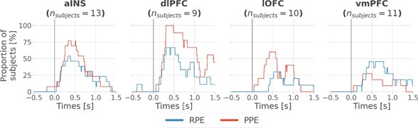
Taken together, we acknowledge a certain variability per region and per condition. Nevertheless, the results presented in the supplementary figures suggest that the main results do not arise from a minority of subjects.
We would like to point out that in order to assess across-subject variability, a much larger number of participants would have been needed, given the low signal-to-noise ratios observed at the single-participant level. We thus prefer to add these results as supplementary material in the Appendix, rather than in the main text.
It is unclear if the findings in Figures 3 and 4 truly reflect the differential interregional dynamics in reward versus punishment learning or if these results arise as a statistical byproduct of the reward vs punishment bias observed within each region. For instance, the authors show that information transfer from anterior insula to dorsolateral prefrontal cortex is specific to punishment prediction error. However, both anterior insula and dorsolateral prefrontal cortex have higher prevalence of punishment prediction error selective electrodes to begin with. Therefore the findings in Fig 3 may simply be reflecting the prevalence of punishment specificity in these two regions above and beyond a punishment specific neural interaction between the two regions. Either mathematical or analytical evidence that assesses if the interaction effect is simply reflecting the local dynamics would be important to make this result convincing.
This is an important point that we partly addressed in the manuscript. More precisely, we investigated whether the synergistic effects observed between the dlPFC and vmPFC encoding global PEs (Fig. 5) could be explained by their respective local specificity. Indeed, since we reported larger proportions of recordings encoding the PPE in the dlPFC and the RPE in the vmPFC (Fig. 2B), we checked whether the synergy between dlPFC and vmPFC could be mainly due to complementary roles where the dlPFC brings information about the PPE only and the vmPFC brings information to the RPE only. To address this point, we selected PPE-specific bipolar derivations from the dlPFC and RPE-specific from the vmPFC and, as the reviewer predicted, we found synergistic II between the two regions probably mainly because of their respective specificity. In addition, we included the II estimated between non-selective bipolar derivations (i.e. recordings with significant encoding for both RPE and PPE) and we observed synergistic interactions (Fig. 5C and Fig. S9). Taken together, the local specificity certainly plays a role, but this is not the only factor in defining the type of interactions.
Concerning the interaction information results (II, Fig. 3), several lines of evidence suggest that local specificity cannot account alone for the II effects. For example, the local specificity for PPE is observed across all four areas (Fig. 2A) and the percentage of bipolar derivations displaying an effect is large (equal or above 10%) for three brain regions (aINS, dlPLF and lOFC). If the local specificity were the main driving cause, we would have observed significant redundancy between all pairs of brain regions. On the other hand, the interaction between the aINS and lOFC displayed no significant redundant effect (Fig. 3B). Another example is the result observed in lOFC: approximately 30% of bipolar derivations display a selectivity for PPE (Fig. 2B, third panel from the left), but do not show clear signs of redundant encoding at the level of within-area interactions (Fig. 3A, bottom-left panel). Similarly, the local encoding for RPE is observed across all four brain regions (Fig. 2A) and the percentage of bipolar derivations displaying an effect is large (equal or above 10%) for three brain regions (aINS, dlPLF and vmPFC). Nevertheless, significant between-regions interactions have been observed only between the lOFC and vmPFC (Fig. 3B bottom right panel).
To further support the reasoning, we performed a simulation to show that it is possible to observe synergistic interactions between two regions with the same specificity. As an example, we may consider one region locally encoding early trials of RPE and a second region encoding the late trials of the RPE. Combining the two with the II would lead to synergistic interactions, because each one of them carries information that is not carried by the other. To illustrate this point, we simulated the data of two regions (x and y). To simulate redundant interactions (first row), each region receives a copy of the prediction (one-to-all) and for the synergy (second row), x and y receive early and late PE trials, respectively (all-to-one). This toy example illustrates that the local specificity is not the only factor determining the type of their interactions. We added the following result to the Appendix.
Author response image 4.
Local specificity does not fully determine the type of interactions. Within-area local encoding of PE using the mutual information (MI, in bits) for regions X and Y and between-area interaction information (II, in bits) leading to (A) redundant interactions and (B) synergistic interactions about the PE
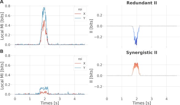
Regarding the information transfer results (Fig. 4), similar arguments hold and suggest that the prevalence is not the main factor explaining the arising transfer entropy between the anterior insula (aINS) and dorsolateral prefrontal cortex (dlPFC). Indeed, the lOFC has a strong local specificity for PPE, but the transfer entropy between the lOFC and aINS (or dlPFC) is shown in Fig. S7 does not show significant differences in encoding between PPE and RPE.
Indeed, such transfer can only be found when there is a delay between the gamma activity of the two regions. In this example, the transfer entropy quantifies the amount of information shared between the past activity of the aINS and the present activity of the dlPFC conditioned on the past activity of the dlPFC. The conditioning ensures that the present activity of the dlPFC is not only explained by its own past. Consequently, if both regions exhibit various prevalences toward reward and punishment but without delay (i.e. at the same timing), the transfer entropy would be null because of the conditioning. As a fact, between 10 to -20% of bipolar recordings show a selectivity to the reward PE (represented by a proportion of 40-60% of subjects, Fig.S4). However, the transfer entropy estimated from the aINS to the dlPFC across rewarding trials is flat and clearly non-significant. If the transfer entropy was a byproduct of the local specificity then we should observe an increase, which is not the case here.
Reviewer #2:
Summary:
Reward and punishment learning have long been seen as emerging from separate networks of frontal and subcortical areas, often studied separately. Nevertheless, both systems are complimentary and distributed representations of rewards and punishments have been repeatedly observed within multiple areas. This raised the unsolved question of the possible mechanisms by which both systems might interact, which this manuscript went after. The authors skillfully leveraged intracranial recordings in epileptic patients performing a probabilistic learning task combined with model-based information theoretical analyses of gamma activities to reveal that information about reward and punishment was not only distributed across multiple prefrontal and insular regions, but that each system showed specific redundant interactions. The reward subsystem was characterized by redundant interactions between orbitofrontal and ventromedial prefrontal cortex, while the punishment subsystem relied on insular and dorsolateral redundant interactions. Finally, the authors revealed a way by which the two systems might interact, through synergistic interaction between ventromedial and dorsolateral prefrontal cortex.
Strengths:
Here, the authors performed an excellent reanalysis of a unique dataset using innovative approaches, pushing our understanding on the interaction at play between prefrontal and insular cortex regions during learning. Importantly, the description of the methods and results is truly made accessible, making it an excellent resource to the community.
This manuscript goes beyond what is classically performed using intracranial EEG dataset, by not only reporting where a given information, like reward and punishment prediction errors, is represented but also by characterizing the functional interactions that might underlie such representations. The authors highlight the distributed nature of frontal cortex representations and propose new ways by which the information specifically flows between nodes. This work is well placed to unify our understanding of the complementarity and specificity of the reward and punishment learning systems.
We thank the reviewer for the positive feedback. Please find below our answers to the weaknesses raised by the reviewer.
Weaknesses:
The conclusions of this paper are mostly supported by the data, but whether the findings are entirely generalizable would require further information/analyses.
First, the authors found that prediction errors very quickly converge toward 0 (less than 10 trials) while subjects performed the task for sets of 96 trials. Considering all trials, and therefore having a non-uniform distribution of prediction errors, could potentially bias the various estimates the authors are extracting. Separating trials between learning (at the start of a set) and exploiting periods could prove that the observed functional interactions are specific to the learning stages, which would strengthen the results.
We thank the reviewer for this question. We would like to note that the probabilistic nature of the learning task does not allow a strict distinction between the exploration and exploitation phases. Indeed, the probability of obtaining the less rewarding outcome was 25% (i.e., for 0€ gain in the reward learning condition and -1€ loss in the punishment learning condition). Thus, participants tended to explore even during the last set of trials in each session. This is evident from the average learning curves shown in Fig. 1B of (Gueguen et al., 2021). Learning curves show rates of correct choice (75% chance of 1€ gain) in the reward condition (blue curves) and incorrect choice (75% chance of 1€ loss) in the punishment condition (red curves).
For what concerns the evolution of PEs, as reviewer #1 suggested, we added a new figure representing the single-subject estimates of the R/PPE (Fig S2). Here, the confidence interval is obtained across all pairs of stimuli presented during the different sessions. We retrieved the general trend of the R/PPE converging toward zero around 10 trials. Both average reward and punishment prediction errors converge toward zero in approximately 10 trials, single-participant curves display large variability, also at the end of each session. As a reminder, the 96 trials represent the total number of trials for one session for the four pairs and the number of trials for each stimulus was only 24.
Author response image 5.
Single-subject estimation of predictions errors. Single-subject trial-wise reward PE (RPE - blue) and punishment PE (PPE - red), ± 95% confidence interval
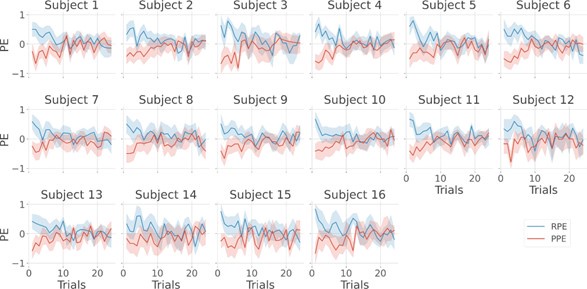
However, the convergence of the R/PPE is due to the average across the pairs of stimuli. In the figure below, we superimposed the estimated R/PPE, per pair of stimuli, for each subject. It becomes very clear that high values of PE can be reached, even for late trials. Therefore, we believe that the split into early/late trials because of the convergence of PE is far from being trivial.
Author response image 6.
Single-subject estimation of predictions errors per pair of stimuli. Single-subject trial-wise reward PE (RPE - blue) and punishment PE (PPE - red)
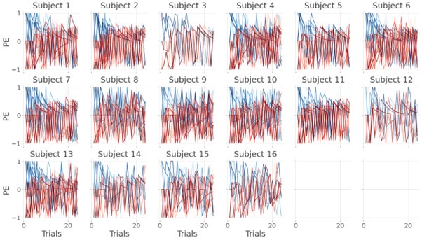
Consequently, nonzero PRE and PPE occur during the whole session and separating trials between learning (at the start of a set) and exploiting periods, as suggested by the reviewer, does not allow a strict dissociation between learning vs no-learning. Nevertheless, we tested the analysis proposed by the reviewer, at the local level. We splitted the 24 trials of each pair of stimuli into early, middle and late trials (8 trials each). We then reproduced Fig. 2 by computing the mutual information between the gamma activity and the R/PPE for subsets of trials: early (first row) and late trials (second row). We retrieved significant encoding of both R/PPE in the aINS, dlPFC and lOFC in both early and late trials. The vmPFC also showed significant encoding of both during early trials. The only difference emerges in the late trials of the vmPFC where we found a strong encoding of the RPE only. It should also be noted that here since we are sub-selecting the trials, the statistical analyses are only performed using a third of the trials.
Taken together, the combination of high values of PE achieved even for late trials and the fact that most of the findings are reproduced even with a third of the trials does not justify the split into early and late trials here. Crucially, this latest analysis confirms that the neural correlates of learning that we observed reflect PE signals rather than early versus late trials in the session.
Author response image 7.
MI between gamma activity and R/PPE using early and late trials. Time courses of MI estimated between the gamma power and both RPE (blue) and PPE (red) using either early or late trials (first and second row, respectively). Horizontal thick lines represent significant clusters of information (p<0.05, cluster-based correction, non-parametric randomization across epochs).
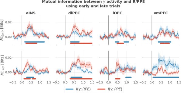
Importantly, it is unclear whether the results described are a common feature observed across subjects or the results of a minority of them. The authors should report and assess the reliability of each result across subjects. For example, the authors found RPE-specific interactions between vmPFC and lOFC, even though less than 10% of sites represent RPE or both RPE/PPE in lOFC. It is questionable whether such a low proportion of sites might come from different subjects, and therefore whether the interactions observed are truly observed in multiple subjects. The nature of the dataset obviously precludes from requiring all subjects to show all effects (given the known limits inherent to intracerebral recording in patients), but it should be proven that the effects were reproducibly seen across multiple subjects.
We thank the reviewer for this remark that has also been raised by the first reviewer. This issue was raised by the first reviewer. Indeed, we added a supplementary figure describing the number of unique subjects per brain region and per pair of brain regions (Fig. S1A) such as the number of bipolar derivations per region and per subject (Fig. S1B).
Author response image 8.
Single subject anatomical repartition. (A) Number of unique subject per brain region and per pair of brain regions (B) Number of bipolar derivations per subject and per brain region
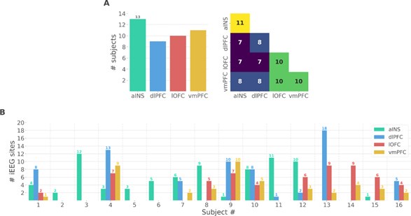
Regarding the reproducibility of the results across subjects for the local analysis (Fig. 2), we also added the instantaneous proportion of subjects having at least one bipolar derivation showing a significant encoding of the RPE and PPE (Fig. S4). We found a minimum proportion of approximately 30% of unique subjects having the effect in the lOFC and vmPFC, respectively with the RPE and PPE. On the other hand, both the aINS and dlPFC showed between 50 to 100% of the subjects having the effect. Therefore, local encoding of RPE and PPE was never represented by a single subject.
Author response image 9.

Similarly, we performed statistical analysis on interaction information at the single-subject level and counted the proportion of unique subjects having at least one pair of recordings with significant redundant and synergistic interactions about the RPE and PPE (Fig. S5). Consistently with the results shown in Fig. 3, the proportions of significant redundant and synergistic interactions are negative and positive, respectively. For the within-regions interactions, approximately 60% of the subjects with redundant interactions are about R/PPE in the aINS and about the PPE in the dlPFC and 40% about the RPE in the vmPFC. For the across-regions interactions, 60% of the subjects have redundant interactions between the aINS-dlPFC and dlPFC-lOFC about the PPE, and 30% have redundant interactions between lOFC-vmPFC about the RPE. Globally, we reproduced the main results shown in Fig. 3.
Author response image 10.
Inter-subjects reproducibility of redundant interactions about PE signals. Time-courses of proportion of subjects having at least one pair of bipolar derivation with a significant interaction information (p<0.05, cluster-based correction, non-parametric randomization across epochs) about the RPE (blue) or PPE (red). Data are aligned to the outcome presentation (vertical line at 0 seconds). Proportion of subjects with redundant (solid) and synergistic (dashed) interactions are respectively going downward and upward.
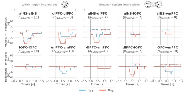
Finally, the timings of the observed interactions between areas preclude one of the authors' main conclusions. Specifically, the authors repeatedly concluded that the encoding of RPE/PPE signals are "emerging" from redundancy-dominated prefrontal-insular interactions. However, the between-region information and transfer entropy between vmPFC and lOFC for example is observed almost 500ms after the encoding of RPE/PPE in these regions, questioning how it could possibly lead to the encoding of RPE/PPE. It is also noteworthy that the two information measures, interaction information and transfer entropy, between these areas happened at non overlapping time windows, questioning the underlying mechanism of the communication at play (see Figures 3/4). As an aside, when assessing the direction of information flow, the authors also found delays between pairs of signals peaking at 176ms, far beyond what would be expected for direct communication between nodes. Discussing this aspect might also be of importance as it raises the possibility of third-party involvement.
The local encoding of RPE in the vmPFC and lOFC is observed in a time interval ranging from approximately 0.2-0.4s to 1.2-1.4s after outcome presentation (blue bars in Fig. 2A). The encoding of RPE by interaction information covers a time interval from approximately 1.1s to 1.5s (blue bars in Fig. 3B, bottom right panel). Similarly, significant TE modulations between the vmPFC and lOFC specific for PPE occur mainly in the 0.7s-1.1s range. Thus, it seems that the local encoding of PPE precedes the effects observed at the level of the neural interactions (II and TE). On the other hand, the modulations in MI, II and TE related to PPE co-occur in a time window from 0.2s to 0.7s after outcome presentation. Thus, we agree with the reviewer that a generic conclusion about the potential mechanisms relating the three levels of analysis cannot be drawn. We thus replaced the term “emerge from” by “occur with” from the manuscript which may be misinterpreted as hinting at a potential mechanism. We nevertheless concluded that the three levels of analysis (and phenomena) co-occur in time, thus hinting at a potential across-scales interaction that needs further study. Indeed, our study suggests that further work, beyond the scope of the current study, is required to better understand the interaction between scales.
Regarding the delay for the conditioning of the transfer entropy, the value of 176 ms reflects the delay at which we observed a maximum of transfer entropy. However, we did not use a single delay for conditioning, we used every possible delay between [116, 236] ms, as explained in the Method section. We would like to stress that transfer entropy is a directed metric of functional connectivity, and it can only be interpreted as quantifying statistical causality defined in terms of predictacìbility according to the Wiener-Granger principle, as detailed in the methods. Thus, it cannot be interpreted in Pearl’s causal terms and as indexing any type of direct communication between nodes. This is a known limitation of the method, which has been stressed in past literature and that we believe does not need to be addressed here.
To account for this, we revised the discussion to make sure this issue is addressed in the following paragraph:
“Here, we quantified directional relationships between regions using the transfer entropy (Schreiber, 2000), which is a functional connectivity measure based on the Granger-Wiener causality principle. Tract tracing studies in the macaque have revealed strong interconnections between the lOFC and vmPFC in the macaque (Carmichael and Price, 1996; Öngür and Price, 2000). In humans, cortico-cortical anatomical connections have mainly been investigated using diffusion magnetic resonance imaging (dMRI). Several studies found strong probabilities of structural connectivity between the anterior insula with the orbitofrontal cortex and dorsolateral part of the prefrontal cortex (Cloutman et al., 2012; Ghaziri et al., 2017), and between the lOFC and vmPFC (Heather Hsu et al., 2020). In addition, the statistical dependency (e.g. coherence) between the LFP of distant areas could be potentially explained by direct anatomical connections (Schneider et al., 2021; Vinck et al., 2023). Taken together, the existence of an information transfer might rely on both direct or indirect structural connectivity. However, here we also reported differences of TE between rewarding and punishing trials given the same backbone anatomical connectivity (Fig. 4). [...] “
Reviewer #3:
Summary:
The authors investigated that learning processes relied on distinct reward or punishment outcomes in probabilistic instrumental learning tasks were involved in functional interactions of two different cortico-cortical gamma-band modulations, suggesting that learning signals like reward or punishment prediction errors can be processed by two dominated interactions, such as areas lOFC-vmPFC and areas aINS-dlPFC, and later on integrated together in support of switching conditions between reward and punishment learning. By performing the well-known analyses of mutual information, interaction information, and transfer entropy, the conclusion was accomplished by identifying directional task information flow between redundancy-dominated and synergy-dominated interactions. Also, this integral concept provided a unifying view to explain how functional distributed reward and/or punishment information were segregated and integrated across cortical areas.
Strengths:
The dataset used in this manuscript may come from previously published works (Gueguen et al., 2021) or from the same grant project due to the methods. Previous works have shown strong evidence about why gamma-band activities and those 4 areas are important. For further analyses, the current manuscript moved the ideas forward to examine how reward/punishment information transfer between recorded areas corresponding to the task conditions. The standard measurements such mutual information, interaction information, and transfer entropy showed time-series activities in the millisecond level and allowed us to learn the directional information flow during a certain window. In addition, the diagram in Figure 6 summarized the results and proposed an integral concept with functional heterogeneities in cortical areas. These findings in this manuscript will support the ideas from human fMRI studies and add a new insight to electrophysiological studies with the non-human primates.
We thank the reviewer for the summary such as for highlighting the strengths. Please find below our answers regarding the weaknesses of the manuscript.
Weaknesses:
After reading through the manuscript, the term "non-selective" in the abstract confused me and I did not actually know what it meant and how it fits the conclusion. If I learned the methods correctly, the 4 areas were studied in this manuscript because of their selective responses to the RPE and PPE signals (Figure 2). The redundancy- and synergy-dominated subsystems indicated that two areas shared similar and complementary information, respectively, due to the negative and positive value of interaction information (Page 6). For me, it doesn't mean they are "non-selective", especially in redundancy-dominated subsystem. I may miss something about how you calculate the mutual information or interaction information. Could you elaborate this and explain what the "non-selective" means?
In the study performed by Gueguen et al. in 2021, the authors used a general linear model (GLM) to link the gamma activity to both the reward and punishment prediction errors and they looked for differences between the two conditions. Here, we reproduced this analysis except that we used measures from the information theory (mutual information) that were able to capture linear and non-linear relationships (although monotonic) between the gamma activity and the prediction errors. The clusters we reported reflect significant encoding of either the RPE and/or the PPE. From Fig. 2, it can be seen that the four regions have a gamma activity that is modulated according to both reward and punishment PE. We used the term “non-selective”, because the regions did not encode either one or the other, but various proportions of bipolar derivations encoding either one or both of them.
The directional information flows identified in this manuscript were evidenced by the recording contacts of iEEG with levels of concurrent neural activities to the task conditions. However, are the conclusions well supported by the anatomical connections? Is it possible that the information was transferred to the target via another area? These questions may remain to be elucidated by using other approaches or animal models. It would be great to point this out here for further investigation.
We thank the reviewer for this interesting question. We added the following paragraph to the discussion to clarify the current limitations of the transfer entropy and the link with anatomical connections :
“Here, we quantified directional relationships between regions using the transfer entropy (Schreiber, 2000), which is a functional connectivity measure based on the Granger-Wiener causality principle. Tract tracing studies in the macaque have revealed strong interconnections between the lOFC and vmPFC in the macaque (Carmichael and Price, 1996; Öngür and Price, 2000). In humans, cortico-cortical anatomical connections have mainly been investigated using diffusion magnetic resonance imaging (dMRI). Several studies found strong probabilities of structural connectivity between the anterior insula with the orbitofrontal cortex and dorsolateral part of the prefrontal cortex (Cloutman et al., 2012; Ghaziri et al., 2017), and between the lOFC and vmPFC (Heather Hsu et al., 2020). In addition, the statistical dependency (e.g. coherence) between the LFP of distant areas could be potentially explained by direct anatomical connections (Schneider et al., 2021). Taken together, the existence of an information transfer might rely on both direct or indirect structural connectivity. However, here we also reported differences of TE between rewarding and punishing trials given the same backbone anatomical connectivity (Fig. 4). Our results are further supported by a recent study involving drug-resistant epileptic patients with resected insula who showed poorer performance than healthy controls in case of risky loss compared to risky gains (Von Siebenthal et al., 2017).”
References
Carmichael ST, Price J. 1996. Connectional networks within the orbital and medial prefrontal cortex of macaque monkeys. J Comp Neurol 371:179–207.
Cloutman LL, Binney RJ, Drakesmith M, Parker GJM, Lambon Ralph MA. 2012. The variation of function across the human insula mirrors its patterns of structural connectivity: Evidence from in vivo probabilistic tractography. NeuroImage 59:3514–3521. oi:10.1016/j.neuroimage.2011.11.016
Combrisson E, Allegra M, Basanisi R, Ince RAA, Giordano BL, Bastin J, Brovelli A. 2022. Group-level inference of information-based measures for the analyses of cognitive brain networks from neurophysiological data. NeuroImage 258:119347. doi:10.1016/j.neuroimage.2022.119347
Ghaziri J, Tucholka A, Girard G, Houde J-C, Boucher O, Gilbert G, Descoteaux M, Lippé S, Rainville P, Nguyen DK. 2017. The Corticocortical Structural Connectivity of the Human Insula. Cereb Cortex 27:1216–1228. doi:10.1093/cercor/bhv308
Gueguen MCM, Lopez-Persem A, Billeke P, Lachaux J-P, Rheims S, Kahane P, Minotti L, David O, Pessiglione M, Bastin J. 2021. Anatomical dissociation of intracerebral signals for reward and punishment prediction errors in humans. Nat Commun 12:3344. doi:10.1038/s41467-021-23704-w
Heather Hsu C-C, Rolls ET, Huang C-C, Chong ST, Zac Lo C-Y, Feng J, Lin C-P. 2020. Connections of the Human Orbitofrontal Cortex and Inferior Frontal Gyrus. Cereb Cortex 30:5830–5843. doi:10.1093/cercor/bhaa160
Lachaux J-P, Fonlupt P, Kahane P, Minotti L, Hoffmann D, Bertrand O, Baciu M. 2007. Relationship between task-related gamma oscillations and BOLD signal: new insights from combined fMRI and intracranial EEG. Hum Brain Mapp 28:1368–1375. doi:10.1002/hbm.20352
Mukamel R, Gelbard H, Arieli A, Hasson U, Fried I, Malach R. 2004. Coupling Between Neuronal Firing, Field Potentials, and fMRI in Human Auditory Cortex. Cereb Cortex 14:881.
Niessing J, Ebisch B, Schmidt KE, Niessing M, Singer W, Galuske RA. 2005. Hemodynamic signals correlate tightly with synchronized gamma oscillations. science 309:948–951.
Nir Y, Fisch L, Mukamel R, Gelbard-Sagiv H, Arieli A, Fried I, Malach R. 2007. Coupling between neuronal firing rate, gamma LFP, and BOLD fMRI is related to interneuronal correlations. Curr Biol 17:1275–1285.
Öngür D, Price JL. 2000. The organization of networks within the orbital and medial prefrontal cortex of rats, monkeys and humans. Cereb Cortex 10:206–219.
Schneider M, Broggini AC, Dann B, Tzanou A, Uran C, Sheshadri S, Scherberger H, Vinck M. 2021. A mechanism for inter-areal coherence through communication based on connectivity and oscillatory power. Neuron 109:4050-4067.e12. doi:10.1016/j.neuron.2021.09.037
Schreiber T. 2000. Measuring information transfer. Phys Rev Lett 85:461.
Von Siebenthal Z, Boucher O, Rouleau I, Lassonde M, Lepore F, Nguyen DK. 2017. Decision-making impairments following insular and medial temporal lobe resection for drug-resistant epilepsy. Soc Cogn Affect Neurosci 12:128–137. doi:10.1093/scan/nsw152
Recommendations for the authors
Reviewer #1
(1) Overall, the writing of the manuscript is dense and makes it hard to follow the scientific logic and appreciate the key findings of the manuscript. I believe the manuscript would be accessible to a broader audience if the authors improved the writing and provided greater detail for their scientific questions, choice of analysis, and an explanation of their results in simpler terms.
We extensively modified the introduction to better describe the rationale and research question.
(2) In the introduction the authors state "we hypothesized that reward and punishment learning arise from complementary neural interactions between frontal cortex regions". This stated hypothesis arrives rather abruptly after a summary of the literature given that the literature summary does not directly inform their stated hypothesis. Put differently, the authors should explicitly state what the contradictions and/or gaps in the literature are, and what specific combinations of findings guide them to their hypothesis. When the authors state their hypothesis the reader is still left asking: why are the authors focusing on the frontal regions? What do the authors mean by complementary interactions? What specific evidence or contradiction in the literature led them to hypothesize that complementary interactions between frontal regions underlie reward and punishment learning?
We extensively modified the introduction and provided a clearer description of the brain circuits involved and the rationale for searching redundant and synergistic interactions between areas.
(3) Related to the above point: when the authors subsequently state "we tested whether redundancy- or synergy dominated interactions allow the emergence of collective brain networks differentially supporting reward and punishment learning", the Introduction (up to the point of this sentence) has not been written to explain the synergy vs. redundancy framework in the literature and how this framework comes into play to inform the authors' hypothesis on reward and punishment learning.
We extensively modified the introduction and provided a clearer description of redundant and synergistic interactions between areas.
(4) The explanation of redundancy vs synergy dominated brain networks itself is written densely and hard to follow. Furthermore, how this framework informs the question on the neural substrates of reward versus punishment learning is unclear. The authors should provide more precise statements on how and why redundancy vs. synergy comes into play in reward and punishment learning. Put differently, this redundancy vs. synergy framework is key for understanding the manuscript and the introduction is not written clearly enough to explain the framework and how it informs the authors' hypothesis and research questions on the neural substrates of reward vs. punishment learning.
Same as above
(5) While the choice of these four brain regions in context of reward and punishment learning does makes sense, the authors do not outline a clear scientific justification as to why these regions were selected in relation to their question.
Same as above
(6) Could the authors explain why they used gamma band power (as opposed to or in addition to the lower frequency bands) to investigate MI. Relatedly, when the authors introduce MI analysis, it would be helpful to briefly explain what this analysis measures and why it is relevant to address the question they are asking.
Please see our answer to the first public comment. We added a paragraph to the discussion section to justify our choice of focusing on the gamma band only. We added the following sentence to the result section to justify our choice for using mutual-information:
The MI allowed us to detect both linear and non-linear relationships between the gamma activity and the PE
An extended explanation justifying our choice for the MI was already present in the method section.
(7) The authors state that "all regions displayed a local "probabilistic" encoding of prediction errors with temporal dynamics peaking around 500 ms after outcome presentation". It would be helpful for the reader if the authors spelled out what they mean by probabilistic in this context as the term can be interpreted in many different ways.
We agree with the reviewer that the term “probabilistic” can be interpreted in different ways. In the revised manuscript we changed “probabilistic” for “mixed”.
(8) The authors should include a brief description of how they compute RPE and PPE in the beginning of the relevant results section.
The explanation of how we estimated the PE is already present in the result section: “We estimated trial-wise prediction errors by fitting a Q-learning model to behavioral data. Fitting the model consisted in adjusting the constant parameters to maximize the likelihood of observed choices etc.”
(9) It is unclear from the Methods whether the authors have taken any measures to address the likely difference in the number of electrodes across subjects. For example, it is likely that some subjects have 10 electrodes in vmPFC while others may have 20. In group analyses, if the data is simply averaged across all electrodes then each subject contributes a different number of data points to the analysis. Hence, a subject with more electrodes can bias the group average. A starting point would be to state the variation in number of electrodes across subjects per brain region. If this variation is rather small, then simple averaging across electrodes might be justified. If the variation is large then one idea would be to average data across electrodes within subjects prior to taking the group average or use a resampling approach where the minimum number of electrodes per brain area is subsampled.
We addressed this point in our public answers. As a reminder, the new version of the manuscript contains a figure showing the number of unique patients per region, the PE at per participant level together with local-encoding at the single participant level.
(10) One thing to consider is whether the reward and punishment in the task is symmetrical in valence. While 1$ increase and 1$ decrease is equivalent in magnitude, the psychological effect of the positive (vs. the negative) outcome may still be asymmetrical and the direction and magnitude of this asymmetry can vary across individuals. For instance, some subjects may be more sensitive to the reward (over punishment) while others are more sensitive to the punishment (over reward). In this scenario, it is possible that the differentiation observed in PPE versus RPE signals may arise from such psychological asymmetry rather than the intrinsic differences in how certain brain regions (and their interactions) may encode for reward vs punishment. Perhaps the authors can comment on this possibility, and/or conduct more in depth behavioral analysis to determine if certain subjects adjust their choice behavior faster in response to reward vs. punishment contexts.
While it could be possible that individuals display different sensitivities vis-à-vis positive and negative prediction errors (and, indeed, a vast body of human reinforcement learning literature seems to point in this direction; Palminteri & Lebreton, 2022), it is unclear to us how such differences would explain into the recruitment of anatomically distinct areas reward and punishment prediction errors. It is important to note here that our design partially orthogonalized positive and reward vs. negative and punishment PEs, because the neutral outcome can generate both positive and negative prediction errors, as a function of the learning context (reward-seeking and punishment avoidance). Back to the main question, for instance, Lefebvre et al (2017) investigated with fMRI the neural correlates of reward prediction errors only and found that inter-individual differences in learning rates for positive and negative prediction errors correlated with differences in the degree of striatal activation and not with the recruitment of different areas. To sum up, while we acknowledge that individuals may display different sensitivity to prediction errors (and reward magnitudes), we believe that such differences should translated in difference in the degree of activation of a given system (the reward systems vs the punishment one) rather than difference in neural system recruitment
(11) As summarized in Fig 6, the authors show that information transfer between aINS to dlPFC was PPE specific whereas the information transfer between vmPFC to lOFC was RPE specific. What is unclear is if these findings arise as an inevitable statistical byproduct of the fact that aINS has high PPE-specificity and that vmPFC has high RPE-specificity. In other words, it is possible that the analysis in Fig 3,4 are sensitive to fact that there is a larger proportion of electrodes with either PPE or RPE sensitivity in aINS and vmPFC respectively - and as such, the II analysis might reflect the dominant local encoding properties above and beyond reflecting the interactions between regions per se. Simply put, could the analysis in Fig 3B turn out in any other way given that there are more PPE specific electrodes in aINS and more RPE specific electrodes in vmPFC? Some options to address this question would be to limit the electrodes included in the analyses (in Fig 3B for example) so that each region has the same number of PPE and RPE specific electrodes included.
Please see the simulation we added to the revised manuscript (Fig. S10) demonstrating that synergistic interactions can emerge between regions with the same specificity.
Regarding the possibility that Fig. 3 and 4 are sensitive to the number of bipolar derivations being R/PPE specific, a counter-example is the vmPFC. The vmPFC has a few recordings specific to punishment (Fig. 2) in almost 30% of the subjects (Fig. S4). However, there is no II about the PPE between recordings of the vmPFC (Fig. 3). The same reasoning also holds for the lOFC. Therefore, the proportion of recordings being RPE or PPE-specific is not sufficient to determine the type of interactions.
(12) Related to the point above, what would the results presented in Fig 3A (and 3B) look like if the authors ran the analyses on RPE specific and PPE specific electrodes only. Is the vmPFC-vmPFC RPE effect in Fig 3A arising simply due to the high prevalence of RPE specific electrodes in vmPFC (as shown in Fig. 2)?
Please see our answer above.
Reviewer #2:
Regarding Figure 2A, the authors argued that their findings "globally reproduced their previously published findings" (from Gueguen et al, 2021). It is worth noting though that in their original analysis, both aINS and lOFC show differential effects (aINS showing greater punishment compared to reward, and the opposite for lOFC) compared to the current analysis. Although I would be akin to believe that the nonlinear approach used here might explain part of the differences (as the authors discussed), I am very wary of the other argument advanced: "the removal of iEEG sites contaminated with pathological activity". This raised some red flags. Does that mean some of the conclusions observed in Gueguen et al (2021) are only the result of noise contamination, and therefore should be disregarded? The author might want to add a short supplementary figure using the same approach as in Gueguen (2021) but using the subset of contacts used here to comfort potential readers of the validity of their previous manuscript.
We appreciate the reviewer's concerns and understand the request for additional information. However, we would like to point out that the figure suggested by the reviewer is already present in the supplementary files of Gueguen et al. 2021 (see Fig. S2). The results of this study should not be disregarded, as the supplementary figure reproduces the results of the main text after excluding sites with pathological activity. Including or excluding sites contaminated with epileptic activity does not have a significant impact on the results, as analyses are performed at each time-stamp and across trials, and epileptic spikes are never aligned in time across trials.
That being said, there are some methodological differences between the two studies. To extract gamma power, Gueguen et al. filtered and averaged 10 Hz sub-bands, while we used multi-tapers. Additionally, they used a temporal smoothing of 250 ms, while we used less smoothing. However, as explained in the main text, we used information-theoretical approaches to capture the statistical dependencies between gamma power and PE. Despite divergent methodologies, we obtained almost identical results.
The data and code supporting this manuscript should be made available. If raw data cannot be shared for ethical reasons, single-trial gamma activities should at least be provided. Regarding the code used to process the data, sharing it could increase the appeal (and use) of the methods applied.
We thank the reviewer for this suggestion. We added a section entitled “Code and data availability” and gave links to the scripts, notebooks and preprocessed data.
Author response:
The following is the authors’ response to the previous reviews.
Recommendations for the authors:
Reviewer #2 (Recommendations for the authors):
I appreciate the efforts the authors made to clarify and justify their statements and methodology, respectively. I additionally appreciate the efforts they made to provide me with detailed information - including figures - to aid my comprehension. However, there are two things I nevertheless recommend the authors to include in the main manuscript.
(1) Statement about animal wellbeing: The authors state that they were constrained in their imaging session duration not because of a commonly reported technical limitation, such as photobleaching (which I honestly assumed), but rather the general wellbeing of the animals, who exhibited signs of distress after longer imaging periods. I find this to be a critical issue and perhaps the best argument against performing longer imaging experiments (which would have increased the number of trials, thus potentially boosting the performance of their model). To say that they put animal welfare above all other scientific and technical considerations speaks to a strong ethical adherence to animal welfare policy, and I believe this should be somehow incorporated into the methods.
We have now included this at the top of page 26:
“Mice fully recovered from the brief isoflurane anesthesia, showing a clear blinking reflex, whisking and sniffing behaviors and normal body posture and movements, immediately after head fixation. In our experimental conditions, mice were imaged in sessions of up to 25 min since beyond this time we started observing some signs of distress or discomfort. Thus, we avoided longer recording times at the expense of collecting larger trial numbers, in strong adherence of animal welfare and ethics policy. A pilot group of mice were habituated to the head fixed condition in daily 20 min sessions for 3 days, however we did not observe a marked contrast in the behavior of habituated versus unhabituated mice beyond our relatively short 25 min imaging sessions. In consequence imaging sessions never surpassed a maximum of 25 min, after which the mouse was returned to its home cage.”
(2) Author response image 2: I sincerely thank the authors for providing us reviewers with this figure, which compares the performance of the naïve Bayesian classifier their ultimately use in the study with other commonly implemented models. Also here I falsely assumed that other models, which take correlated activity into account, did not generally perform better than their ultimate model of choice. Although dwelling on it would be distractive (and outside the primary scope of the study), I would encourage the authors to include it as a figure supplement (and simply mention these controls en passant when they justify their choice of the naïve Bayesian classifier).
This figure was now included in the revised manuscript as supplemental figure 3.
Page 10 now reads:
“We performed cross-validated, multi-class classification of the single-trial population responses (decoding, Fig. 2A) using a naive Bayes classifier to evaluate the prediction errors as the absolute difference between the stimulus azimuth and the predicted azimuth (Fig. 2A). We chose this classification algorithm over others due to its generally good performance with limited available data. We visualized the cross-validated prediction error distribution in cumulative plots where the observed prediction errors were compared to the distribution of errors for random azimuth sampling (Fig. 2B). When decoding all simultaneously recorded units, the observed classifier output was not significantly better (shifted towards smaller prediction errors) than the chance level distribution (Fig. 2B). The classifier also failed to decode complete DCIC population responses recorded with neuropixels probes (Fig. 3A). Other classifiers performed similarly (Suppl. Fig. 3A).”
The bottom paragraph in page 19 now reads:
“To characterize how the observed positive noise correlations could affect the representation of stimulus azimuth by DCIC top ranked unit population responses, we compared the decoding performance obtained by classifying the single-trial response patterns from top ranked units in the modeled decorrelated datasets versus the acquired data (with noise correlations). With the intention to characterize this with a conservative approach that would be less likely to find a contribution of noise correlations as it assumes response independence, we relied on the naive Bayes classifier for decoding throughout the study. Using this classifier, we observed that the modeled decorrelated datasets produced stimulus azimuth prediction error distributions that were significantly shifted towards higher decoding errors (Fig. 6B, C) and, in our imaging datasets, were not significantly different from chance level (Fig. 6B). Altogether, these results suggest that the detected noise correlations in our simultaneously acquired datasets can help reduce the error of the IC population code for sound azimuth. We observed a similar, but not significant tendency with another classifier that does not assume response independence (KNN classifier), though overall producing larger decoding errors than the Bayes classifier (Suppl. Fig. 3B).”
Reviewer #3 (Recommendations for the authors):
I am generally happy with the response to the reviews.
I find the Author response image 3 quite interesting. The neuropixel data looks somewhat like I expected (especially for mouse #3 and maybe mouse #4). I find the distribution of weights across units in the imaging dataset compared to in the pixel dataset intriguing (though it probably is just the dimensionality of the data being so much higher).
I'm not too familiar with facial movements but is it the case that the DCIC would be more modulated by ipsilateral movement compared to contralateral movements? Are face movements in mice conjugate or do both sides of the face move more or less independently? If not it may be interesting in future work to record bilaterally and see if that provides more information about DCIC responses.
We sincerely thank the editors and reviewers for their careful appraisal, commendation of our effort and helpful constructive feedback which greatly improved the presentation of our study. Below in green font is a point by point reply to the comments provided by the reviewers.
Public Reviews:
Reviewer #1 (Public Review):
Summary: In this study, the authors address whether the dorsal nucleus of the inferior colliculus (DCIC) in mice encodes sound source location within the front horizontal plane (i.e., azimuth). They do this using volumetric two-photon Ca2+ imaging and high-density silicon probes (Neuropixels) to collect single-unit data. Such recordings are beneficial because they allow large populations of simultaneous neural data to be collected. Their main results and the claims about those results are the following:
(1) DCIC single-unit responses have high trial-to-trial variability (i.e., neural noise);
(2) approximately 32% to 40% of DCIC single units have responses that are sensitive to sound source azimuth;
(3) single-trial population responses (i.e., the joint response across all sampled single units in an animal) encode sound source azimuth "effectively" (as stated in title) in that localization decoding error matches average mouse discrimination thresholds;
(4) DCIC can encode sound source azimuth in a similar format to that in the central nucleus of the inferior colliculus (as stated in Abstract);
(5) evidence of noise correlation between pairs of neurons exists;
and (6) noise correlations between responses of neurons help reduce population decoding error.
While simultaneous recordings are not necessary to demonstrate results #1, #2, and #4, they are necessary to demonstrate results #3, #5, and #6.
Strengths:
- Important research question to all researchers interested in sensory coding in the nervous system.
- State-of-the-art data collection: volumetric two-photon Ca2+ imaging and extracellular recording using high-density probes. Large neuronal data sets.
- Confirmation of imaging results (lower temporal resolution) with more traditional microelectrode results (higher temporal resolution).
- Clear and appropriate explanation of surgical and electrophysiological methods. I cannot comment on the appropriateness of the imaging methods.
Strength of evidence for claims of the study:
(1) DCIC single-unit responses have high trial-to-trial variability - The authors' data clearly shows this.
(2) Approximately 32% to 40% of DCIC single units have responses that are sensitive to sound source azimuth - The sensitivity of each neuron's response to sound source azimuth was tested with a Kruskal-Wallis test, which is appropriate since response distributions were not normal. Using this statistical test, only 8% of neurons (median for imaging data) were found to be sensitive to azimuth, and the authors noted this was not significantly different than the false positive rate. The Kruskal-Wallis test was not performed on electrophysiological data. The authors suggested that low numbers of azimuth-sensitive units resulting from the statistical analysis may be due to the combination of high neural noise and relatively low number of trials, which would reduce statistical power of the test. This may be true, but if single-unit responses were moderately or strongly sensitive to azimuth, one would expect them to pass the test even with relatively low statistical power. At best, if their statistical test missed some azimuthsensitive units, they were likely only weakly sensitive to azimuth. The authors went on to perform a second test of azimuth sensitivity-a chi-squared test-and found 32% (imaging) and 40% (e-phys) of single units to have statistically significant sensitivity. This feels a bit like fishing for a lower p-value. The Kruskal-Wallis test should have been left as the only analysis. Moreover, the use of a chi-squared test is questionable because it is meant to be used between two categorical variables, and neural response had to be binned before applying the test.
The determination of what is a physiologically relevant “moderate or strong azimuth sensitivity” is not trivial, particularly when comparing tuning across different relays of the auditory pathway like the CNIC, auditory cortex, or in our case DCIC, where physiologically relevant azimuth sensitivities might be different. This is likely the reason why azimuth sensitivity has been defined in diverse ways across the bibliography (see Groh, Kelly & Underhill, 2003 for an early discussion of this issue). These diverse approaches include reaching a certain percentage of maximal response modulation, like used by Day et al. (2012, 2015, 2016) in CNIC, and ANOVA tests, like used by Panniello et al. (2018) and Groh, Kelly & Underhill (2003) in auditory cortex and IC respectively. Moreover, the influence of response variability and biases in response distribution estimation due to limited sampling has not been usually accounted for in the determination of azimuth sensitivity.
As Reviewer #1 points out, in our study we used an appropriate ANOVA test (KruskalWallis) as a starting point to study response sensitivity to stimulus azimuth at DCIC. Please note that the alpha = 0.05 used for this test is not based on experimental evidence about physiologically relevant azimuth sensitivity but instead is an arbitrary p-value threshold. Using this test on the electrophysiological data, we found that ~ 21% of the simultaneously recorded single units reached significance (n = 4 mice). Nevertheless these percentages, in our small sample size (n = 4) were not significantly different from our false positive detection rate (p = 0.0625, Mann-Whitney, See Author response image 1). In consequence, for both our imaging (Fig. 3C) and electrophysiological data, we could not ascertain if the percentage of neurons reaching significance in these ANOVA tests were indeed meaningfully sensitive to azimuth or this was due to chance.
Author response image 1.
Percentage of the neuropixels recorded DCIC single units across mice that showed significant median response tuning, compared to false positive detection rate (α = 0.05, chance level).
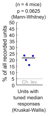
We reasoned that the observed markedly variable responses from DCIC units, which frequently failed to respond in many trials (Fig. 3D, 4A), in combination with the limited number of trial repetitions we could collect, results in under-sampled response distribution estimations. This under-sampling can bias the determination of stochastic dominance across azimuth response samples in Kruskal-Wallis tests. We would like to highlight that we decided not to implement resampling strategies to artificially increase the azimuth response sample sizes with “virtual trials”, in order to avoid “fishing for a smaller p-value”, when our collected samples might not accurately reflect the actual response population variability.
As an alternative to hypothesis testing based on ranking and determining stochastic dominance of one or more azimuth response samples (Kruskal-Wallis test), we evaluated the overall statistical dependency to stimulus azimuth of the collected responses. To do this we implement the Chi-square test by binning neuronal responses into categories. Binning responses into categories can reduce the influence of response variability to some extent, which constitutes an advantage of the Chi-square approach, but we note the important consideration that these response categories are arbitrary.
Altogether, we acknowledge that our Chi-square approach to define azimuth sensitivity is not free of limitations and despite enabling the interrogation of azimuth sensitivity at DCIC, its interpretability might not extend to other brain regions like CNIC or auditory cortex. Nevertheless we hope the aforementioned arguments justify why the Kruskal-Wallis test simply could not “have been left as the only analysis”.
(3) Single-trial population responses encode sound source azimuth "effectively" in that localization decoding error matches average mouse discrimination thresholds - If only one neuron in a population had responses that were sensitive to azimuth, we would expect that decoding azimuth from observation of that one neuron's response would perform better than chance. By observing the responses of more than one neuron (if more than one were sensitive to azimuth), we would expect performance to increase. The authors found that decoding from the whole population response was no better than chance. They argue (reasonably) that this is because of overfitting of the decoder modeltoo few trials used to fit too many parameters-and provide evidence from decoding combined with principal components analysis which suggests that overfitting is occurring. What is troubling is the performance of the decoder when using only a handful of "topranked" neurons (in terms of azimuth sensitivity) (Fig. 4F and G). Decoder performance seems to increase when going from one to two neurons, then decreases when going from two to three neurons, and doesn't get much better for more neurons than for one neuron alone. It seems likely there is more information about azimuth in the population response, but decoder performance is not able to capture it because spike count distributions in the decoder model are not being accurately estimated due to too few stimulus trials (14, on average). In other words, it seems likely that decoder performance is underestimating the ability of the DCIC population to encode sound source azimuth.
To get a sense of how effective a neural population is at coding a particular stimulus parameter, it is useful to compare population decoder performance to psychophysical performance. Unfortunately, mouse behavioral localization data do not exist. Therefore, the authors compare decoder error to mouse left-right discrimination thresholds published previously by a different lab. However, this comparison is inappropriate because the decoder and the mice were performing different perceptual tasks. The decoder is classifying sound sources to 1 of 13 locations from left to right, whereas the mice were discriminating between left or right sources centered around zero degrees. The errors in these two tasks represent different things. The two data sets may potentially be more accurately compared by extracting information from the confusion matrices of population decoder performance. For example, when the stimulus was at -30 deg, how often did the decoder classify the stimulus to a lefthand azimuth? Likewise, when the stimulus was +30 deg, how often did the decoder classify the stimulus to a righthand azimuth?
The azimuth discrimination error reported by Lauer et al. (2011) comes from engaged and highly trained mice, which is a very different context to our experimental setting with untrained mice passively listening to stimuli from 13 random azimuths. Therefore we did not perform analyses or interpretations of our results based on the behavioral task from Lauer et al. (2011) and only made the qualitative observation that the errors match for discussion.
We believe it is further important to clarify that Lauer et al. (2011) tested the ability of mice to discriminate between a positively conditioned stimulus (reference speaker at 0º center azimuth associated to a liquid reward) and a negatively conditioned stimulus (coming from one of five comparison speakers positioned at 20º, 30º, 50º, 70 and 90º azimuth, associated to an electrified lickport) in a conditioned avoidance task. In this task, mice are not precisely “discriminating between left or right sources centered around zero degrees”, making further analyses to compare the experimental design of Lauer et al (2011) and ours even more challenging for valid interpretation.
(4) DCIC can encode sound source azimuth in a similar format to that in the central nucleus of the inferior colliculus - It is unclear what exactly the authors mean by this statement in the Abstract. There are major differences in the encoding of azimuth between the two neighboring brain areas: a large majority of neurons in the CNIC are sensitive to azimuth (and strongly so), whereas the present study shows a minority of azimuth-sensitive neurons in the DCIC. Furthermore, CNIC neurons fire reliably to sound stimuli (low neural noise), whereas the present study shows that DCIC neurons fire more erratically (high neural noise).
Since sound source azimuth is reported to be encoded by population activity patterns at CNIC (Day and Delgutte, 2013), we refer to a population activity pattern code as the “similar format” in which this information is encoded at DCIC. Please note that this is a qualitative comparison and we do not claim this is the “same format”, due to the differences the reviewer precisely describes in the encoding of azimuth at CNIC where a much larger majority of neurons show stronger azimuth sensitivity and response reliability with respect to our observations at DCIC. By this qualitative similarity of encoding format we specifically mean the similar occurrence of activity patterns from azimuth sensitive subpopulations of neurons in both CNIC and DCIC, which carry sufficient information about the stimulus azimuth for a sufficiently accurate prediction with regard to the behavioral discrimination ability.
(5) Evidence of noise correlation between pairs of neurons exists - The authors' data and analyses seem appropriate and sufficient to justify this claim.
(6) Noise correlations between responses of neurons help reduce population decoding error - The authors show convincing analysis that performance of their decoder increased when simultaneously measured responses were tested (which include noise correlation) than when scrambled-trial responses were tested (eliminating noise correlation). This makes it seem likely that noise correlation in the responses improved decoder performance. The authors mention that the naïve Bayesian classifier was used as their decoder for computational efficiency, presumably because it assumes no noise correlation and, therefore, assumes responses of individual neurons are independent of each other across trials to the same stimulus. The use of decoder that assumes independence seems key here in testing the hypothesis that noise correlation contains information about sound source azimuth. The logic of using this decoder could be more clearly spelled out to the reader. For example, if the null hypothesis is that noise correlations do not carry azimuth information, then a decoder that assumes independence should perform the same whether population responses are simultaneous or scrambled. The authors' analysis showing a difference in performance between these two cases provides evidence against this null hypothesis.
We sincerely thank the reviewer for this careful and detailed consideration of our analysis approach. Following the reviewer’s constructive suggestion, we justified the decoder choice in the results section at the last paragraph of page 18:
“To characterize how the observed positive noise correlations could affect the representation of stimulus azimuth by DCIC top ranked unit population responses, we compared the decoding performance obtained by classifying the single-trial response patterns from top ranked units in the modeled decorrelated datasets versus the acquired data (with noise correlations). With the intention to characterize this with a conservative approach that would be less likely to find a contribution of noise correlations as it assumes response independence, we relied on the naive Bayes classifier for decoding throughout the study.
Using this classifier, we observed that the modeled decorrelated datasets produced stimulus azimuth prediction error distributions that were significantly shifted towards higher decoding errors (Fig. 5B, C) and, in our imaging datasets, were not significantly different from chance level (Fig. 5B). Altogether, these results suggest that the detected noise correlations in our simultaneously acquired datasets can help reduce the error of the IC population code for sound azimuth.”
Minor weakness:
- Most studies of neural encoding of sound source azimuth are done in a noise-free environment, but the experimental setup in the present study had substantial background noise. This complicates comparison of the azimuth tuning results in this study to those of other studies. One is left wondering if azimuth sensitivity would have been greater in the absence of background noise, particularly for the imaging data where the signal was only about 12 dB above the noise. The description of the noise level and signal + noise level in the Methods should be made clearer. Mice hear from about 2.5 - 80 kHz, so it is important to know the noise level within this band as well as specifically within the band overlapping with the signal.
We agree with the reviewer that this information is useful. In our study, the background R.M.S. SPL during imaging across the mouse hearing range (2.5-80kHz) was 44.53 dB and for neuropixels recordings 34.68 dB. We have added this information to the methods section of the revised manuscript.
Reviewer #2 (Public Review):
In the present study, Boffi et al. investigate the manner in which the dorsal cortex of the of the inferior colliculus (DCIC), an auditory midbrain area, encodes sound location azimuth in awake, passively listening mice. By employing volumetric calcium imaging (scanned temporal focusing or s-TeFo), complemented with high-density electrode electrophysiological recordings (neuropixels probes), they show that sound-evoked responses are exquisitely noisy, with only a small portion of neurons (units) exhibiting spatial sensitivity. Nevertheless, a naïve Bayesian classifier was able to predict the presented azimuth based on the responses from small populations of these spatially sensitive units. A portion of the spatial information was provided by correlated trial-to-trial response variability between individual units (noise correlations). The study presents a novel characterization of spatial auditory coding in a non-canonical structure, representing a noteworthy contribution specifically to the auditory field and generally to systems neuroscience, due to its implementation of state-of-the-art techniques in an experimentally challenging brain region. However, nuances in the calcium imaging dataset and the naïve Bayesian classifier warrant caution when interpreting some of the results.
Strengths:
The primary strength of the study lies in its methodological achievements, which allowed the authors to collect a comprehensive and novel dataset. While the DCIC is a dorsal structure, it extends up to a millimetre in depth, making it optically challenging to access in its entirety. It is also more highly myelinated and vascularised compared to e.g., the cerebral cortex, compounding the problem. The authors successfully overcame these challenges and present an impressive volumetric calcium imaging dataset. Furthermore, they corroborated this dataset with electrophysiological recordings, which produced overlapping results. This methodological combination ameliorates the natural concerns that arise from inferring neuronal activity from calcium signals alone, which are in essence an indirect measurement thereof.
Another strength of the study is its interdisciplinary relevance. For the auditory field, it represents a significant contribution to the question of how auditory space is represented in the mammalian brain. "Space" per se is not mapped onto the basilar membrane of the cochlea and must be computed entirely within the brain. For azimuth, this requires the comparison between miniscule differences between the timing and intensity of sounds arriving at each ear. It is now generally thought that azimuth is initially encoded in two, opposing hemispheric channels, but the extent to which this initial arrangement is maintained throughout the auditory system remains an open question. The authors observe only a slight contralateral bias in their data, suggesting that sound source azimuth in the DCIC is encoded in a more nuanced manner compared to earlier processing stages of the auditory hindbrain. This is interesting, because it is also known to be an auditory structure to receive more descending inputs from the cortex.
Systems neuroscience continues to strive for the perfection of imaging novel, less accessible brain regions. Volumetric calcium imaging is a promising emerging technique, allowing the simultaneous measurement of large populations of neurons in three dimensions. But this necessitates corroboration with other methods, such as electrophysiological recordings, which the authors achieve. The dataset moreover highlights the distinctive characteristics of neuronal auditory representations in the brain. Its signals can be exceptionally sparse and noisy, which provide an additional layer of complexity in the processing and analysis of such datasets. This will be undoubtedly useful for future studies of other less accessible structures with sparse responsiveness.
Weaknesses:
Although the primary finding that small populations of neurons carry enough spatial information for a naïve Bayesian classifier to reasonably decode the presented stimulus is not called into question, certain idiosyncrasies, in particular the calcium imaging dataset and model, complicate specific interpretations of the model output, and the readership is urged to interpret these aspects of the study's conclusions with caution.
I remain in favour of volumetric calcium imaging as a suitable technique for the study, but the presently constrained spatial resolution is insufficient to unequivocally identify regions of interest as cell bodies (and are instead referred to as "units" akin to those of electrophysiological recordings). It remains possible that the imaging set is inadvertently influenced by non-somatic structures (including neuropil), which could report neuronal activity differently than cell bodies. Due to the lack of a comprehensive ground-truth comparison in this regard (which to my knowledge is impossible to achieve with current technology), it is difficult to imagine how many informative such units might have been missed because their signals were influenced by spurious, non-somatic signals, which could have subsequently misled the models. The authors reference the original Nature Methods article (Prevedel et al., 2016) throughout the manuscript, presumably in order to avoid having to repeat previously published experimental metrics. But the DCIC is neither the cortex nor hippocampus (for which the method was originally developed) and may not have the same light scattering properties (not to mention neuronal noise levels). Although the corroborative electrophysiology data largely eleviates these concerns for this particular study, the readership should be cognisant of such caveats, in particular those who are interested in implementing the technique for their own research.
A related technical limitation of the calcium imaging dataset is the relatively low number of trials (14) given the inherently high level of noise (both neuronal and imaging). Volumetric calcium imaging, while offering a uniquely expansive field of view, requires relatively high average excitation laser power (in this case nearly 200 mW), a level of exposure the authors may have wanted to minimise by maintaining a low the number of repetitions, but I yield to them to explain.
We assumed that the levels of heating by excitation light measured at the neocortex in Prevedel et al. (2016), were representative for DCIC also. Nevertheless, we recognize this approximation might not be very accurate, due to the differences in tissue architecture and vascularization from these two brain areas, just to name a few factors. The limiting factor preventing us from collecting more trials in our imaging sessions was that we observed signs of discomfort or slight distress in some mice after ~30 min of imaging in our custom setup, which we established as a humane end point to prevent distress. In consequence imaging sessions were kept to 25 min in duration, limiting the number of trials collected. However we cannot rule out that with more extensive habituation prior to experiments the imaging sessions could be prolonged without these signs of discomfort or if indeed influence from our custom setup like potential heating of the brain by illumination light might be the causing factor of the observed distress. Nevertheless, we note that previous work has shown that ~200mW average power is a safe regime for imaging in the cortex by keeping brain heating minimal (Prevedel et al., 2016), without producing the lasting damages observed by immunohistochemisty against apoptosis markers above 250mW (Podgorski and Ranganathan 2016, https://doi.org/10.1152/jn.00275.2016).
Calcium imaging is also inherently slow, requiring relatively long inter-stimulus intervals (in this case 5 s). This unfortunately renders any model designed to predict a stimulus (in this case sound azimuth) from particularly noisy population neuronal data like these as highly prone to overfitting, to which the authors correctly admit after a model trained on the entire raw dataset failed to perform significantly above chance level. This prompted them to feed the model only with data from neurons with the highest spatial sensitivity. This ultimately produced reasonable performance (and was implemented throughout the rest of the study), but it remains possible that if the model was fed with more repetitions of imaging data, its performance would have been more stable across the number of units used to train it. (All models trained with imaging data eventually failed to converge.) However, I also see these limitations as an opportunity to improve the technology further, which I reiterate will be generally important for volume imaging of other sparse or noisy calcium signals in the brain.
Transitioning to the naïve Bayesian classifier itself, I first openly ask the authors to justify their choice of this specific model. There are countless types of classifiers for these data, each with their own pros and cons. Did they actually try other models (such as support vector machines), which ultimately failed? If so, these negative results (even if mentioned en passant) would be extremely valuable to the community, in my view. I ask this specifically because different methods assume correspondingly different statistical properties of the input data, and to my knowledge naïve Bayesian classifiers assume that predictors (neuronal responses) are assumed to be independent within a class (azimuth). As the authors show that noise correlations are informative in predicting azimuth, I wonder why they chose a model that doesn't take advantage of these statistical regularities. It could be because of technical considerations (they mention computing efficiency), but I am left generally uncertain about the specific logic that was used to guide the authors through their analytical journey.
One of the main reasons we chose the naïve Bayesian classifier is indeed because it assumes that the responses of the simultaneously recorded neurons are independent and therefore it does not assume a contribution of noise correlations to the estimation of the posterior probability of each azimuth. This model would represent the null hypothesis that noise correlations do not contribute to the encoding of stimulus azimuth, which would be verified by an equal decoding outcome from correlated or decorrelated datasets. Since we observed that this is not the case, the model supports the alternative hypothesis that noise correlations do indeed influence stimulus azimuth encoding. We wanted to test these hypotheses with the most conservative approach possible that would be least likely to find a contribution of noise correlations. Other relevant reasons that justify our choice of the naive Bayesian classifier are its robustness against the limited numbers of trials we could collect in comparison to other more “data hungry” classifiers like SVM, KNN, or artificial neuronal nets. We did perform preliminary tests with alternative classifiers but the obtained decoding errors were similar when decoding the whole population activity (Supplemental figure 3A). Dimensionality reduction following the approach described in the manuscript showed a tendency towards smaller decoding errors observed with an alternative classifier like KNN, but these errors were still larger than the ones observed with the naive Bayesian classifier (median error 45º). Nevertheless, we also observe a similar tendency for slightly larger decoding errors in the absence of noise correlations (decorrelated, Supplemental figure 3B). Sentences detailing the logic of classifier choice are now included in the results section at page 10 and at the last paragraph of page 18 (see responses to Reviewer 1).
That aside, there remain other peculiarities in model performance that warrant further investigation. For example, what spurious features (or lack of informative features) in these additional units prevented the models of imaging data from converging?
Considering the amount of variability observed throughout the neuronal responses both in imaging and neuropixels datasets, it is easy to suspect that the information about stimulus azimuth carried in different amounts by individual DCIC neurons can be mixed up with information about other factors (Stringer et al., 2019). In an attempt to study the origin of these features that could confound stimulus azimuth decoding we explored their relation to face movement (Supplemental Figure 2), finding a correlation to snout movements, in line with previous work by Stringer et al. (2019).
In an orthogonal question, did the most spatially sensitive units share any detectable tuning features? A different model trained with electrophysiology data in contrast did not collapse in the range of top-ranked units plotted. Did this model collapse at some point after adding enough units, and how well did that correlate with the model for the imaging data?
Our electrophysiology datasets were much smaller in size (number of simultaneously recorded neurons) compared to our volumetric calcium imaging datasets, resulting in a much smaller total number of top ranked units detected per dataset. This precluded the determination of a collapse of decoder performance due to overfitting beyond the range plotted in Fig 4G.
How well did the form (and diversity) of the spatial tuning functions as recorded with electrophysiology resemble their calcium imaging counterparts? These fundamental questions could be addressed with more basic, but transparent analyses of the data (e.g., the diversity of spatial tuning functions of their recorded units across the population). Even if the model extracts features that are not obvious to the human eye in traditional visualisations, I would still find this interesting.
The diversity of the azimuth tuning curves recorded with calcium imaging (Fig. 3B) was qualitatively larger than the ones recorded with electrophysiology (Fig. 4B), potentially due to the larger sampling obtained with volumetric imaging. We did not perform a detailed comparison of the form and a more quantitative comparison of the diversity of these functions because the signals compared are quite different, as calcium indicator signal is subject to non linearities due to Ca2+ binding cooperativity and low pass filtering due to binding kinetics. We feared this could lead to misleading interpretations about the similarities or differences between the azimuth tuning functions in imaged and electrophysiology datasets. Our model uses statistical response dependency to stimulus azimuth, which does not rely on features from a descriptive statistic like mean response tuning. In this context, visualizing the trial-to-trial responses as a function of azimuth shows “features that are not obvious to the human eye in traditional visualizations” (Fig. 3D, left inset).
Finally, the readership is encouraged to interpret certain statements by the authors in the current version conservatively. How the brain ultimately extracts spatial neuronal data for perception is anyone's guess, but it is important to remember that this study only shows that a naïve Bayesian classifier could decode this information, and it remains entirely unclear whether the brain does this as well. For example, the model is able to achieve a prediction error that corresponds to the psychophysical threshold in mice performing a discrimination task (~30 {degree sign}). Although this is an interesting coincidental observation, it does not mean that the two metrics are necessarily related. The authors correctly do not explicitly claim this, but the manner in which the prose flows may lead a non-expert into drawing that conclusion.
To avoid misleading the non-expert readers, we have clarified in the manuscript that the observed correspondence between decoding error and psychophysical threshold is explicitly coincidental.
Page 13, end of middle paragraph:
“If we consider the median of the prediction error distribution as an overall measure of decoding performance, the single-trial response patterns from subsamples of at least the 7 top ranked units produced median decoding errors that coincidentally matched the reported azimuth discrimination ability of mice (Fig 4G, minimum audible angle = 31º) (Lauer et al., 2011).”
Page 14, bottom paragraph:
“Decoding analysis (Fig. 4F) of the population response patterns from azimuth dependent top ranked units simultaneously recorded with neuropixels probes showed that the 4 top ranked units are the smallest subsample necessary to produce a significant decoding performance that coincidentally matches the discrimination ability of mice (31° (Lauer et al., 2011)) (Fig. 5F, G).”
We also added to the Discussion sentences clarifying that a relationship between these two variables remains to be determined and it also remains to be determined if the DCIC indeed performs a bayesian decoding computation for sound localization.
Page 20, bottom:
“… Concretely, we show that sound location coding does indeed occur at DCIC on the single trial basis, and that this follows a comparable mechanism to the characterized population code at CNIC (Day and Delgutte, 2013). However, it remains to be determined if indeed the DCIC network is physiologically capable of Bayesian decoding computations. Interestingly, the small number of DCIC top ranked units necessary to effectively decode stimulus azimuth suggests that sound azimuth information is redundantly distributed across DCIC top ranked units, which points out that mechanisms beyond coding efficiency could be relevant for this population code.
While the decoding error observed from our DCIC datasets obtained in passively listening, untrained mice coincidentally matches the discrimination ability of highly trained, motivated mice (Lauer et al., 2011), a relationship between decoding error and psychophysical performance remains to be determined. Interestingly, a primary sensory representations should theoretically be even more precise than the behavioral performance as reported in the visual system (Stringer et al., 2021).”
Moreover, the concept of redundancy (of spatial information carried by units throughout the DCIC) is difficult for me to disentangle. One interpretation of this formulation could be that there are non-overlapping populations of neurons distributed across the DCIC that each could predict azimuth independently of each other, which is unlikely what the authors meant. If the authors meant generally that multiple neurons in the DCIC carry sufficient spatial information, then a single neuron would have been able to predict sound source azimuth, which was not the case. I have the feeling that they actually mean "complimentary", but I leave it to the authors to clarify my confusion, should they wish.
We observed that the response patterns from relatively small fractions of the azimuth sensitive DCIC units (4-7 top ranked units) are sufficient to generate an effective code for sound azimuth, while 32-40% of all simultaneously recorded DCIC units are azimuth sensitive. In light of this observation, we interpreted that the azimuth information carried by the population should be redundantly distributed across the complete subpopulation of azimuth sensitive DCIC units.
In summary, the present study represents a significant body of work that contributes substantially to the field of spatial auditory coding and systems neuroscience. However, limitations of the imaging dataset and model as applied in the study muddles concrete conclusions about how the DCIC precisely encodes sound source azimuth and even more so to sound localisation in a behaving animal. Nevertheless, it presents a novel and unique dataset, which, regardless of secondary interpretation, corroborates the general notion that auditory space is encoded in an extraordinarily complex manner in the mammalian brain.
Reviewer #3 (Public Review):
Summary: Boffi and colleagues sought to quantify the single-trial, azimuthal information in the dorsal cortex of the inferior colliculus (DCIC), a relatively understudied subnucleus of the auditory midbrain. They used two complementary recording methods while mice passively listened to sounds at different locations: a large volume but slow sampling calcium-imaging method, and a smaller volume but temporally precise electrophysiology method. They found that neurons in the DCIC were variable in their activity, unreliably responding to sound presentation and responding during inter-sound intervals. Boffi and colleagues used a naïve Bayesian decoder to determine if the DCIC population encoded sound location on a single trial. The decoder failed to classify sound location better than chance when using the raw single-trial population response but performed significantly better than chance when using intermediate principal components of the population response. In line with this, when the most azimuth dependent neurons were used to decode azimuthal position, the decoder performed equivalently to the azimuthal localization abilities of mice. The top azimuthal units were not clustered in the DCIC, possessed a contralateral bias in response, and were correlated in their variability (e.g., positive noise correlations). Interestingly, when these noise correlations were perturbed by inter-trial shuffling decoding performance decreased. Although Boffi and colleagues display that azimuthal information can be extracted from DCIC responses, it remains unclear to what degree this information is used and what role noise correlations play in azimuthal encoding.
Strengths: The authors should be commended for collection of this dataset. When done in isolation (which is typical), calcium imaging and linear array recordings have intrinsic weaknesses. However, those weaknesses are alleviated when done in conjunction with one another - especially when the data largely recapitulates the findings of the other recording methodology. In addition to the video of the head during the calcium imaging, this data set is extremely rich and will be of use to those interested in the information available in the DCIC, an understudied but likely important subnucleus in the auditory midbrain.
The DCIC neural responses are complex; the units unreliably respond to sound onset, and at the very least respond to some unknown input or internal state (e.g., large inter-sound interval responses). The authors do a decent job in wrangling these complex responses: using interpretable decoders to extract information available from population responses.
Weaknesses:
The authors observe that neurons with the most azimuthal sensitivity within the DCIC are positively correlated, but they use a Naïve Bayesian decoder which assume independence between units. Although this is a bit strange given their observation that some of the recorded units are correlated, it is unlikely to be a critical flaw. At one point the authors reduce the dimensionality of their data through PCA and use the loadings onto these components in their decoder. PCA incorporates the correlational structure when finding the principal components and constrains these components to be orthogonal and uncorrelated. This should alleviate some of the concern regarding the use of the naïve Bayesian decoder because the projections onto the different components are independent. Nevertheless, the decoding results are a bit strange, likely because there is not much linearly decodable azimuth information in the DCIC responses. Raw population responses failed to provide sufficient information concerning azimuth for the decoder to perform better than chance. Additionally, it only performed better than chance when certain principal components or top ranked units contributed to the decoder but not as more components or units were added. So, although there does appear to be some azimuthal information in the recoded DCIC populations - it is somewhat difficult to extract and likely not an 'effective' encoding of sound localization as their title suggests.
As described in the responses to reviewers 1 and 2, we chose the naïve Bayes classifier as a decoder to determine the influence of noise correlations through the most conservative approach possible, as this classifier would be least likely to find a contribution of correlated noise. Also, we chose this decoder due to its robustness against limited numbers of trials collected, in comparison to “data hungry” non linear classifiers like KNN or artificial neuronal nets. Lastly, we observed that small populations of noisy, unreliable (do not respond in every trial) DCIC neurons can encode stimulus azimuth in passively listening mice matching the discrimination error of trained mice. Therefore, while this encoding is definitely not efficient, it can still be considered effective.
Although this is quite a worthwhile dataset, the authors present relatively little about the characteristics of the units they've recorded. This may be due to the high variance in responses seen in their population. Nevertheless, the authors note that units do not respond on every trial but do not report what percent of trials that fail to evoke a response. Is it that neurons are noisy because they do not respond on every trial or is it also that when they do respond they have variable response distributions? It would be nice to gain some insight into the heterogeneity of the responses.
The limited number of azimuth trial repetitions that we could collect precluded us from making any quantification of the unreliability (failures to respond) and variability in the response distributions from the units we recorded, as we feared they could be misleading. In qualitative terms, “due to the high variance in responses seen” in the recordings and the limited trial sampling, it is hard to make any generalization. In consequence we referred to the observed response variance altogether as neuronal noise. Considering these points, our datasets are publicly available for exploration of the response characteristics.
Additionally, is there any clustering at all in response profiles or is each neuron they recorded in the DCIC unique?
We attempted to qualitatively visualize response clustering using dimensionality reduction, observing different degrees of clustering or lack thereof across the azimuth classes in the datasets collected from different mice. It is likely that the limited number of azimuth trials we could collect and the high response variance contribute to an inconsistent response clustering across datasets.
They also only report the noise correlations for their top ranked units, but it is possible that the noise correlations in the rest of the population are different.
For this study, since our aim was to interrogate the influence of noise correlations on stimulus azimuth encoding by DCIC populations, we focused on the noise correlations from the top ranked unit subpopulation, which likely carry the bulk of the sound location information. Noise correlations can be defined as correlation in the trial to trial response variation of neurons. In this respect, it is hard to ascertain if the rest of the population, that is not in the top rank unit percentage, are really responding and showing response variation to evaluate this correlation, or are simply not responding at all and show unrelated activity altogether. This makes observations about noise correlations from “the rest of the population” potentially hard to interpret.
It would also be worth digging into the noise correlations more - are units positively correlated because they respond together (e.g., if unit x responds on trial 1 so does unit y) or are they also modulated around their mean rates on similar trials (e.g., unit x and y respond and both are responding more than their mean response rate). A large portion of trial with no response can occlude noise correlations. More transparency around the response properties of these populations would be welcome.
Due to the limited number of azimuth trial repetitions collected, to evaluate noise correlations we used the non parametric Kendall tau correlation coefficient which is a measure of pairwise rank correlation or ordinal association in the responses to each azimuth. Positive rank correlation would represent neurons more likely responding together. Evaluating response modulation “around their mean rates on similar trials” would require assumptions about the response distributions, which we avoided due to the potential biases associated with limited sample sizes.
It is largely unclear what the DCIC is encoding. Although the authors are interested in azimuth, sound location seems to be only a small part of DCIC responses. The authors report responses during inter-sound interval and unreliable sound-evoked responses. Although they have video of the head during recording, we only see a correlation to snout and ear movements (which are peculiar since in the example shown it seems the head movements predict the sound presentation). Additional correlates could be eye movements or pupil size. Eye movement are of particular interest due to their known interaction with IC responses - especially if the DCIC encodes sound location in relation to eye position instead of head position (though much of eye-position-IC work was done in primates and not rodent). Alternatively, much of the population may only encode sound location if an animal is engaged in a localization task. Ideally, the authors could perform more substantive analyses to determine if this population is truly noisy or if the DCIC is integrating un-analyzed signals.
We unsuccessfully attempted eye tracking and pupillometry in our videos. We suspect that the reason behind this is a generally overly dilated pupil due to the low visible light illumination conditions we used which were necessary to protect the PMT of our custom scope.
It is likely that DCIC population activity is integrating un-analyzed signals, like the signal associated with spontaneous behaviors including face movements (Stringer et al., 2019), which we observed at the level of spontaneous snout movements. However investigating if and how these signals are integrated to stimulus azimuth coding requires extensive behavioral testing and experimentation which is out of the scope of this study. For the purpose of our study, we referred to trial-to-trial response variation as neuronal noise. We note that this definition of neuronal noise can, and likely does, include an influence from un-analyzed signals like the ones from spontaneous behaviors.
Although this critique is ubiquitous among decoding papers in the absence of behavioral or causal perturbations, it is unclear what - if any - role the decoded information may play in neuronal computations. The interpretation of the decoder means that there is some extractable information concerning sound azimuth - but not if it is functional. This information may just be epiphenomenal, leaking in from inputs, and not used in computation or relayed to downstream structures. This should be kept in mind when the authors suggest their findings implicate the DCIC functionally in sound localization.
Our study builds upon previous reports by other independent groups relying on “causal and behavioral perturbations” and implicating DCIC in sound location learning induced experience dependent plasticity (Bajo et al., 2019, 2010; Bajo and King, 2012), which altogether argues in favor of DCIC functionality in sound localization.
Nevertheless, we clarified in the discussion of the revised manuscript that a relationship between the observed decoding error and the psychophysical performance, or the ability of the DCIC network to perform Bayesian decoding computations, both remain to be determined (please see responses to Reviewer #2).
It is unclear why positive noise correlations amongst similarly tuned neurons would improve decoding. A toy model exploring how positive noise correlations in conjunction with unreliable units that inconsistently respond may anchor these findings in an interpretable way. It seems plausible that inconsistent responses would benefit from strong noise correlations, simply by units responding together. This would predict that shuffling would impair performance because you would then be sampling from trials in which some units respond, and trials in which some units do not respond - and may predict a bimodal performance distribution in which some trials decode well (when the units respond) and poor performance (when the units do not respond).
In samples with more that 2 dimensions, the relationship between signal and noise correlations is more complex than in two dimensional samples (Montijn et al., 2016) which makes constructing interpretable and simple toy models of this challenging. Montijn et al. (2016) provide a detailed characterization and model describing how the accuracy of a multidimensional population code can improve when including “positive noise correlations amongst similarly tuned neurons”. Unfortunately we could not successfully test their model based on Mahalanobis distances as we could not verify that the recorded DCIC population responses followed a multivariate gaussian distribution, due to the limited azimuth trial repetitions we could sample.
Significance: Boffi and colleagues set out to parse the azimuthal information available in the DCIC on a single trial. They largely accomplish this goal and are able to extract this information when allowing the units that contain more information about sound location to contribute to their decoding (e.g., through PCA or decoding on top unit activity specifically). The dataset will be of value to those interested in the DCIC and also to anyone interested in the role of noise correlations in population coding. Although this work is first step into parsing the information available in the DCIC, it remains difficult to interpret if/how this azimuthal information is used in localization behaviors of engaged mice.
Author response:
The following is the authors’ response to the previous reviews
Reviewer #1 (Public review):
Summary:
Ma & Yang et al. report a new investigation aimed at elucidating one of the key nutrients S. Typhimurium (STM) utilizes with the nutrient-poor intracellular niche within macrophage, focusing on the amino acid beta-alanine. From these data, the authors report that beta-alanine plays important roles in mediating STM infection and virulence. The authors employ a multidisciplinary approach that includes some mouse studies, and ultimately propose a mechanism by which panD, involved in B-Ala synthesis, mediates regulation of zinc homeostatisis in Salmonella.
Strengths and weaknesses:
The results and model are adequately supported by the authors' data. Further work will need to be performed to learn whether the Zn2+ functions as proposed in their mechanism. By performing a small set of confirmatory experiments in S. Typhi, the authors provide some evidence of relevance to human infections.
Impact:
This work adds to the body of literature on the metabolic flexibility of Salmonella during infection that enable pathogenesis.
Reviewer #1 (Recommendations for the authors):
No further suggestions. The authors have adequately addressed my prior concerns through new data and revisions to the text.
Thank you for considering this work. We appreciate your efforts in aiding us to improve our manuscript.
Reviewer #3 (Public review):
Summary:
Salmonella is interesting due to its life within a compact compartment, which we call SCV or Salmonella containing vacuole in the field of Salmonella. SCV is a tight-fitting vacuole where the acquisition of nutrients is a key factor by Salmonella. The authors among many nutrients, focussed on beta-alanine. It is also known that Salmonella requires beta-alanine from many other studies. The authors have done in vitro RAW macrophage infection assays and In vivo mouse infection assays to see the life of Salmonella in the presence of beta-alanine. They concluded by comprehending that beta-alanine modulates the expression of many genes including zinc transporters which is required for pathogenesis.
Strengths:
Made a couple of knockouts in Salmonella and did transcriptomic to understand the global gene expression pattern
Weaknesses:
(1) Transport of Beta-alanine to SCV is not yet elucidated. Is it possible to determine whether the Zn transporter is involved in B-alanine transport?
Thank you for the comment. Following your suggestion, we investigated the growth of Salmonella WT and the ∆znuA mutant cultured in N-minimal and M9 minimal medium, with β-alanine as the sole carbon source. We observed no significant difference in growth kinetics between the ∆znuA mutant and WT strain under either culture condition (please refer to Author response image 1). The results indicate that ZnuA is not involved in β-alanine transport in Salmonella.
Author response image 1.
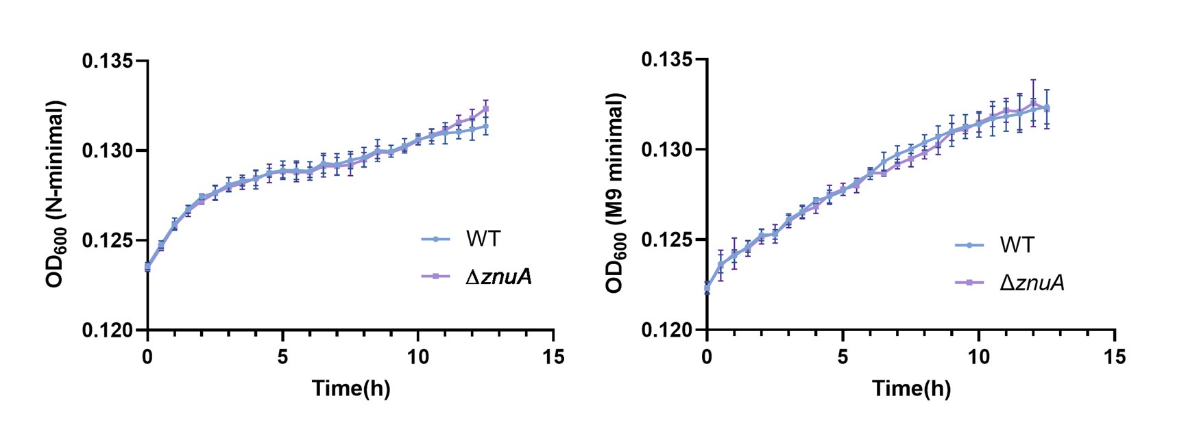
(2) Beta-alanine can also be shuttled to form carnosine along with histidine. If beta-alanine is channelled to make more carnosine, then the virulence phenotypes may be very different.
Our study reveals that β-alanine availability, whether obtained from the host or synthesized de novo via the panD-dependent pathway, is important for Salmonella pathogenesis. We have shown that β-alanine influences Salmonella intracellular replication and in vivo virulence partly by enhancing the expression of the zinc transporter genes.
Although β-alanine can also be shuttled to form carnosine along with histidine in animals, the Salmonella genome lacks canonical carnosine synthase (CARNS) orthologs that catalyze the condensation of β-alanine and histidine into carnosine. Therefore, we believe that the carnosine biosynthetic pathway does not influence the virulence phenotypes of Salmonella.
(3) Some amino acid transporters can be knocked out to see if beta-alanine uptake is perturbed. Like ArgT transport Arginine, and its mutation perturbs the uptake of beta-alanine. What is the beta-alanine concentration in the SCV? SCVS can be purified at different time points, and the Beta-alanine concentration can be measured
Thank you for the comment. As suggested, we have investigated the role of other amino acid transporters in the uptake of β-alanine. In E. coli, GabP transports γ-aminobutyric acid (GABA), a structural analogue of β-alanine, and may also transport β-alanine (J Bacteriol. 2021, 203(4):e00642-20). Nevertheless, Salmonella ∆gabP mutant displayed no growth defect in minimal medium with β-alanine as the sole carbon source (Figure 1_figure Supplement 7, Figure 1_figure Supplement 8), indicating that GabP is not involved in β-alanine uptake in Salmonella. Strikingly, the Δ_argT_ mutant—defective in arginine uptake—showed markedly decreased growth in the minimal medium with β-alanine as the sole carbon source (Figure 1F),suggesting that ArgT also transports β-alanine in Salmonella. We have added the results in the revised manuscript (lines 167-179).
It has been reported that ArgT is essential for Salmonella replication within macrophages and full virulence in vivo (PloS one. 2010, 5(12):e15466). Given that ArgT is involved in both arginine and β-alanine uptake (as verified in this study), whether the attenuated virulence of the ∆argT mutant is due to a deficiency in β-alanine or arginine requires further investigation. We have also included a discussion on this issue (lines 409-415).
In this work, to avoid delays and alterations in metabolite concentrations during the isolation of bacterial contents from macrophages, we directly assessed the combined metabolite concentrations within infected cells and Salmonella. It has been previously verified that these metabolites are primarily of host origin (Nat Commun. 2021, 12(1):879.). We noted a decrease in β-alanine levels in macrophages infected with Salmonella. The process of separating SCV is intricate and encompasses dissociation and sonication (Nat Commun. 2018, 9(1):2091). These steps may potentially result in alterations of metabolite concentrations during the separation procedure. Therefore, we did not measure the β-alanine concentration in the SCV.
Reviewer #3 (Recommendations for the authors):
The Authors have done meticulous experiments to address the questions asked by the reviewers. My one question of beta-alanine transport inside the SCV remains undone, though the authors have tried.
Was Zinc transporter mutant checked? It is possible that the Zn transporter can take up Beta-alanine.
Thank you for the comment. Following your suggestion, we investigated the growth of Salmonella WT and the ∆znuA mutant cultured in N-minimal and M9 minimal medium, with β-alanine as the sole carbon source. We observed no significant difference in growth kinetics between the ∆znuA mutant and WT strain under either culture condition (please refer to Author response image 1). The results indicate that ZnuA is not involved in β-alanine transport in Salmonella.
Additionally, we have investigated the role of other amino acid transporters in the uptake of β-alanine and have ultimately identified that ArgT, the arginine transporter, is involved in the uptake of β-alanine in Salmonella (please refer to our previous response).
Author Response:
The following is the authors’ response to the original reviews.
eLife assessment
This study presents potentially useful findings describing how activity in the corticotropin-releasing hormone neurons in the paraventricular nucleus of the hypothalamus modulates sevoflurane anesthesia, as well as a phenomenon the authors term a "general anesthetic stress response". The technical approaches are solid and the data presented are largely clear. However, the primary conclusion, that the PVHCRH neurons are a mechanism of sevoflurane anesthesia, is inadequately supported.
We appreciate the editors and reviewers for their thorough assessment and constructive feedback. We have provided clarifications and updated the manuscripts to better interpret our results, please see below. As for the primary conclusion, we revised it as PVH CRH neurons potently modulate states of anaesthesia in sevoflurane general anesthesia, being a part of anaesthesia regulatory network of sevoflurane.
Combined Public Review:
This study describes a group of CRH-releasing neurons, located in the paraventricular nucleus of the hypothalamus, which, in mice, affects both the state of sevoflurane anesthesia and a grooming behavior observed after it. PVH-CRH neurons showed elevated calcium activity during the post-anesthesia period. Optogenetic activation of these PVH-CRH neurons during sevoflurane anesthesia shifts the EEG from burst-suppression to a seemingly activated state (an apparent arousal effect), although without a behavioral correlate. Chemogenetic activation of the PVH-CRH neurons delays sevoflurane-induced loss of righting reflex (another apparent arousal effect). On the other hand, chemogenetic inhibition of PVH-CRH neurons delays recovery of the righting reflex and decreases sevoflurane-induced stress (an apparent decrease in the arousal effect). The authors conclude that PVH-CRH neurons are a common substrate for sevoflurane-induced anesthesia and stress. The PVH-CRH neurons are related to behavioral stress responses, and the authors claim that these findings provide direct evidence for a relationship between sevoflurane anesthesia and sevoflurane-mediated stress that might exist even when there is no surgical trauma, such as an incision. In its current form, the article does not achieve its intended goal.
Thank you for the detailed review. We have carefully considered your comments and have revised the manuscript to provide a clearer interpretation of our findings. Our findings indicate that PVH CRH neurons integrate the anesthetic effect and post-anesthesia stress response of sevoflurane (GA), providing new evidence for understanding the neuronal regulation of sevoflurane GA and identifying a potential brain target for further investigation into modulating the post-anesthesia stress response. However, we did not propose that there was a direct relationship between sevoflurane anesthesia and sevoflurane-mediated stress in the absence of incision. Our results mainly concluded that PVH CRH neurons integrate the anaesthetic effect and post-anaesthesia stress response of sevoflurane GA, which offers new evidence for the neuronal regulation of sevoflurane GA and provides an important but ignored potential cause of the post-anesthesia stress response.
Strengths:
The manuscript uses targeted manipulation of the PVH-CRH neurons, and is technically sound. Also, the number of experiments is substantial.
Thank you.
Weaknesses:
The most significant weaknesses are a) the lack of consideration and measurement of GABAergic mechanisms of sevoflurane anesthesia, b) the failure to use another anesthetic as a control, c) a failure to document a compelling post-anesthesia stress response to sevoflurane in humans, d) limitations in the novelty of the findings. These weaknesses are related to the primary concerns described below:
Concerns about the primary conclusion, that PVH-CRH neurons mediate "the anesthetic effects and post-anesthesia stress response of sevoflurane GA".
Thanks for the advice. Our responses are as below:
1) Just because the activity of a given neural cell type or neural circuit alters an anesthetic's response, this does not mean that those neurons play a role in how the anesthetic creates its anesthetic state. For example, sevoflurane is commonly used in children. Its primary mechanism of action is through enhancement of GABA-mediated inhibition. Children with ADHD on Ritalin (a dopamine reuptake inhibitor) who take it on the day of surgery can often require increased doses of sevoflurane to achieve the appropriate anesthetic state. The mesocortical pathway through which Ritalin acts is not part of the mechanism of action of sevoflurane. Through this pathway, Ritalin is simply increasing cortical excitability making it more challenging for the inhibitory effects of sevoflurane at GABAergic synapses to be effective. Similarly, here, altering the activity of the PVHCRH neurons and seeing a change in anesthetic response to sevoflurane does not mean that these neurons play a role in the fundamental mechanism of this anesthetic's action. With the current data set, the primary conclusions should be tempered.
Thank you for your comments. Our results adequately uncover PVH CRH neurons that modulate the state of consciousness as well as the stress response in sevoflurane GA, but are insufficient to demonstrate that these neurons play a role in the underlying mechanism of sevoflurane anesthesia. We will revise our conclusions and make them concrete. The primary conclusion has been revised as PVH CRH neurons potently modulate states of anaesthesia in sevoflurane GA, being a part of the anaesthesia regulatory network of sevoflurane.
2) It is important to compare the effects of sevoflurane with at least one other inhaled ether anesthetic. Isoflurane, desflurane, and enflurane are ether anesthetics that are very similar to each other, as well as being similar to sevoflurane. It is important to distinguish whether the effects of sevoflurane pertain to other anesthetics, or, alternatively, relate to unique idiosyncratic properties of this gas that may not be a part of its anesthetic properties.
For example, one study cited by the authors (Marana et al.. 2013) concludes that there is weak evidence for differences in stress-related hormones between sevoflurane and desflurane, with lower levels of cortisol and ACTH observed during the desflurane intraoperative period. It is not clear that this difference in some stress-related hormones is modeled by post-sevoflurane excess grooming in the mice, but using desflurane as a control could help determine this.
Thank you for your suggestions. We completely agree on the importance of determining whether the effects of sevoflurane apply to other anesthetics or arise from unique idiosyncratic attributes separate from its anesthetic properties. However, it is challenging to definitively conclude whether the effects of sevoflurane observed in our study extend to other inhaled anesthetics, even with desflurane as a control. While sevoflurane shares many common anesthetic properties with other inhalation agents, it also exhibits distinct characteristics and potential idiosyncrasies that set it apart from its counterparts. Regarding studies related to desflurane's impact on hormone levels or stress-like behaviors, one study involving 20 women scheduled for elective total abdominal hysterectomy demonstrated that there was no significant correlation between the intra-operative depth of anesthesia achieved with desflurane and the extent of the endocrine-metabolic stress response (as indicated by the concentrations of plasma cortisol, glucose, and lactate)1. Besides, a study conducted with mice suggested the abilities related to sensorimotor functions, anxiety and depression did not undergo significant changes after 7 days of anesthesia administered with 8.0% desflurane for 6 h2. Furthermore, a study involving 50 Caucasian women undergoing laparoscopic surgery for benign ovarian cysts demonstrated that in low stress surgery, desflurane, when compared to sevoflurane, exhibited superior control over the intraoperative cortisol and ACTH response 3. Based on these findings, we propose that the effect we observed in this study is likely attributed to the unique idiosyncratic properties of sevoflurane. We will conduct additional experiments to investigate this proposal with other commonly used anaesthetics in our future studies.
Concerns about the clinical relevance of the experiments
In anesthesiology practice, perioperative stress observed in patients is more commonly related to the trauma of the surgical intervention, with inadequate levels of antinociception or unconsciousness intraoperatively and/or poor post-operative pain control. The authors seem to be suggesting that the anesthetic itself is causing stress, but there is no evidence of this from human patients cited. We were not aware that this is a documented clinical phenomenon. It is important to know whether sevoflurane effectively produces behavioral stress in the recovery room in patients that could be related to the putative stress response (excess grooming) observed in mice. For example, in surgeries or procedures that required only a brief period of unconsciousness that could be achieved by administering sevoflurane alone (comparable to the 30 min administered to the mice), is there clinical evidence of post-operative stress?
Thank you for your question. There is currently no direct evidence available. Studies on sevoflurane in humans primarily focus on its use during surgical interventions, making it difficult to find studies that solely administer sevoflurane, as was done in our study with mice. Generally, a short anesthesia time refers to procedures that last less than one hour, while a long anesthesia time could be considered for procedures lasting several hours or more4. A study published in eLife investigated the patterns of reemerging consciousness and cognitive function in 30 healthy adults who underwent GA for three hours 5. This finding suggests that the cognitive dysfunction observed immediately and persistently after GA in healthy animals may not necessarily apply anesthesia and postoperative neurocognitive disorders could be influenced by factors other than GA, such as surgery or patient comorbidity. Therefore, further studies are needed to verify the post-operative stress in sevoflurane-only short time anesthesia.
Indeed, stress after surgeries can result from multiple factors aside from anesthesia, including pain, anxiety, inflammation, but what we want to illustrate in this study is that anesthesia could be one of these factors that we ignored in previous studies. In our current study, we did not propose that there was a direct relationship between sevoflurane anesthesia and sevoflurane-mediated stress without incision. We observed stress-related behavioural changes after exposure of sevoflurane GA in mouse model, indicating sevoflurane-mediated stress might exist without surgical trauma. Importantly, whether anesthetic administration alone will cause post-operative stress is worth studying in different species especially human.
Patients who receive sevoflurane as the primary anesthetic do not wake up more stressed than if they had had one of the other GABAergic anesthetics. If there were signs of stress upon emergence (increased heart rate, blood pressure, thrashing movements) from general anesthesia, the anesthesiologist would treat this right away. The most likely cause of post-operative stress behaviors in humans is probably inadequate anti-nociception during the procedure, which translates into inadequate post-op analgesia and likely delirium. It is the case that children receiving sevoflurane do have a higher likelihood of post-operative delirium. Perhaps the authors' studies address a mechanism for delirium associated with sevoflurane, but this is not considered. Delirium seems likely to be the closest clinical phenomenon to what was studied.
We agree with your idea. We aim to establish a connection between post-operative delirium in humans and stress-like behaviors observed in mice following sevoflurane anesthesia. Specifically, we have observed that the increased grooming behavior exhibited by mice after sevoflurane anesthesia resembles the fuzzy state of consciousness experienced during post-operative delirium6. In our discussion, we also emphasized the occurrence of sevoflurane-induced emergence agitation, a common phenomenon reported in clinical studies with an incidence of up to 80%. This state is characterized by hyperactivity, confusion, delirium, and emotional agitation 7,8. Meanwhile, in our experimental tests, namely the open field test (OFT) and elevated plus maze (EPM) test, we observed that mice exposed to sevoflurane inhalation displayed reduced movement distances during both the OFT and EPM tests (Figure 7G and I). These findings suggest a decline in behavioral activity similar to what is observed in cases of delirium.
Concerns about the novelty of the findings
CRH is associated with arousal in numerous studies. In fact, the authors' own work, published in eLife in 2021, showed that stimulating the hypothalamic CRH cells leads to arousal and their inhibition promotes hypersomnia. In both papers, the authors use fos expression in CRH cells during a specific event to implicate the cells, then manipulate them and measure EEG responses. In the previous work, the cells were active during wakefulness; here- they were active in the awake state that follows anesthesia (Figure 1). Thus, the findings in the current work are incremental.
Thank you for acknowledging our previous work focusing on the changes in the sleep-wake state of mice when PVH CRH neurons are manipulated. In this study, our primary objective was to identify the neuronal mechanisms mediating the anesthetic effects and post-anesthetic stress response of sevoflurane GA. While our study claims that activation of PVH CRH neurons leads to arousal, it provides evidence that PVH CRH neurons may play a role in the regulation of conscious states in GA. Our current findings uncover that PVH CRH neurons modulate the state of consciousness as well as the stress response in sevoflurane GA, and that the modulation of PVH CRH neurons bidirectionally altered the induction and recovery of sevoflurane GA. This identifies a new brain region involved in sevoflurane GA that goes beyond the arousal-related regions.
The activation of CRH cells in PVN has already been shown to result in grooming by Jaideep Bains (cited as reference 58). Thus, the involvement of these cells in this behavior is expected. The authors perform elaborate manipulations of CRH cells and numerous analyses of grooming and related behaviors. For example, they compare grooming and paw licking after anesthesia with those after other stressors such as forced swim, spraying mice with water, physical attack, and restraint. However, the relevance of these behaviors to humans and generalization to other types of anesthetics is not clear.
The hyperactivity of PVH CRH neurons and behavior (e.g., excessive self-grooming) in mice may partially mirror the observed agitation and underlying mechanisms during emergence from sevoflurane GA in patients. As mentioned in the Discussion section (page 16, lines 371-374), sevoflurane-induced emergence agitation represents a prevalent manifestation of the post-anesthesia stress response. It is frequently observed, with an incidence of up to 80% in clinical reports, and is characterized by hyperactivity, confusion, delirium, and emotional agitation7,8. Our aim in this study is to distinguish the excessive stress responses of patients to sevoflurane GA from stress triggered by other factors. Other stimuli, such as forced swimming, can be considered sources of both physical and emotional stress, which are associated with depression and anxiety in humans.
Regarding generalization to other types of anesthetics, we propose that the stress-related behavioral effects observed in this study might occur in cases of the administration of certain types of anesthetics. For example, one study showed that intravenous ketamine infusion (10 mg/kg, 2 hours) elevated plasma corticosterone and progesterone levels in rats, reducing locomotor activity (sedation) 9. The administration of intravenous anesthesia with propofol combined with sevoflurane caused greater postoperative stress than the single use of propofol10. However, desflurane, a common inhaled ether anesthetic, when compared to sevoflurane, was associated with better control of intraoperative cortisol and ACTH response in low-stress surgeries8. Thus, these behaviors observed after exposure to sevoflurane GA may be related to the post-anesthesia stress response in humans, which might also occur in cases of the administration of certain types of anesthetics.
Recommendations for the authors:
Reviewer 1
1) The CRH-Cre mouse line should be validated. There are several lines of these mice, and their fidelity varies.
The CRH-Cre mouse line we used in this study is from The Jackson Laboratory (https://www.jax.org/strain/012704) with the name B6(Cg)-Crhtm1(cre)Zjh/J (Strain #: 012704). These CRH-ires-CRE knock-in mice have Cre recombinase expression directed to CRH positive neurons by the endogenous promoter/enhancer elements of the corticotropin releasing hormone locus (Crh). We have done standard PCR to validate the mouse line following genotyping protocols provided by the Jackson Laboratory. The protocol primers were: 10574 (SEQUENCE 5' → 3': CTT ACA CAT TTC GTC CTA GCC); 10575 (SEQUENCE 5' → 3': CAC GAC CAG GCT GCG GCT AAC); 10576 (SEQUENCE 5' → 3': CAA TGT ATC TTA TCA TGT CTG GAT CC). The 468-bp CRH-specific PCR product was amplified in mutant (CRH-Cre+/+) mice; in heterozygote (CRH-Cre+/-) mice, both the 468-bp and the 676-bp PCR products were detected; in wild type (WT) mice, only the 676-bp WT allele-specific PCR product was amplified. An example of PCR results is presented below. The heterozygote and mutant mice were included in our study.
Author response image 1.
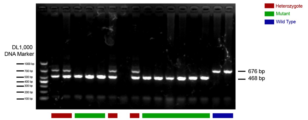
- It would be very helpful to validate the CRH antibody. Using any antiserum at 1:800 suggests that it may not be potent or highly specific.
As requested, we used the same CRH antibody at a concentration of 1:800, following the methods described in the Method section. The results are displayed below.
Author response image 2.
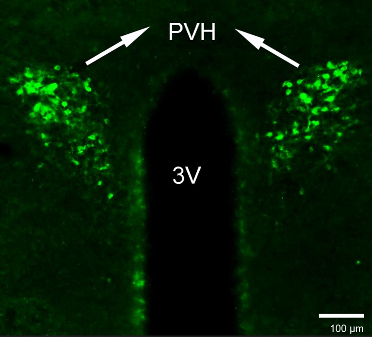
- In Figure 1C, the control sections are out of focus, any cells are blurry, reducing confidence in the analyses (locus ceruleus cells appear confluent in the control?)
Sorry for the confusing figure and we have revised the control section part of Figure 1C:
Author response image 3.
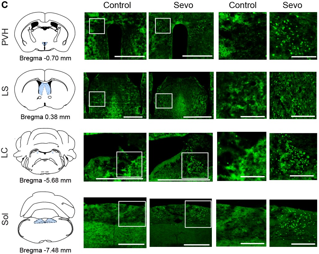
Reviewer 2
1) In the Abstract, to say that "General anesthetics benefit patients undergoing surgeries without consciousness. ..." is a gross understatement of the essential role that general anesthesia plays today to make surgery not only tolerable but humane. This opening sentence should be rewritten. General anesthesia is a fundamental process required to undertake safely and humanely a high fraction of surgeries and invasive diagnostic procedures.
As requested, we rewrote this opening sentence, please see the follows:
GA is a fundamental process required to undertake surgeries and invasive diagnostic procedures safely and humanely. However, the undesired stress response associated with GA can lead to delayed recovery and even increased morbidity in clinical settings.
2) In the Abstract, when discussing the response of the PVN-CRH neurons to chemogenetic inhibition, say exactly what the "opposite effect" is.
Thanks for your insights. We have rewritten our abstract as follows:
Chemogenetic activation of these neurons delayed the induction and accelerated emergence from sevoflurane GA, whereas chemogenetic inhibition of PVH CRH neurons promoted induction and prolonged emergence from sevoflurane GA.
3) In all spectrograms the dynamic range is compressed between 0.5 and 1. Please make use of the full range, as some details might be missed because of this compression.
We are sorry for the incorrect unit of the spectrograms. We have provided the correct one with full range, please see below:
Author response image 4.
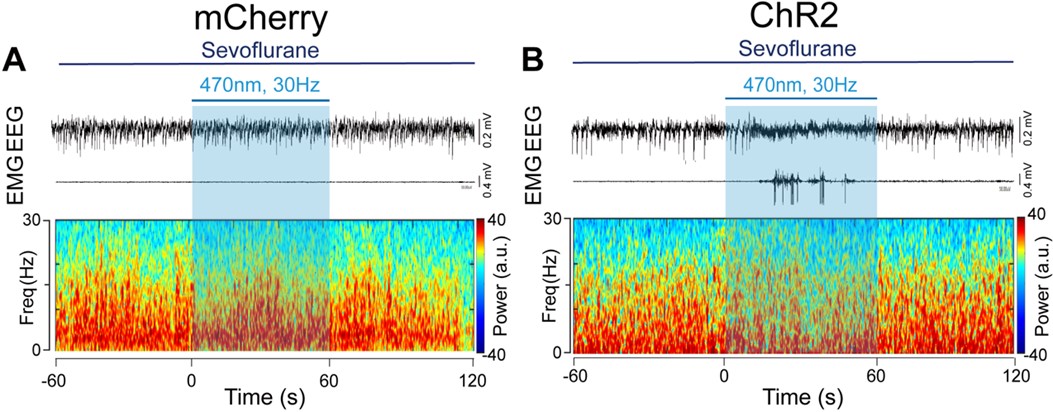
Author response image 5.
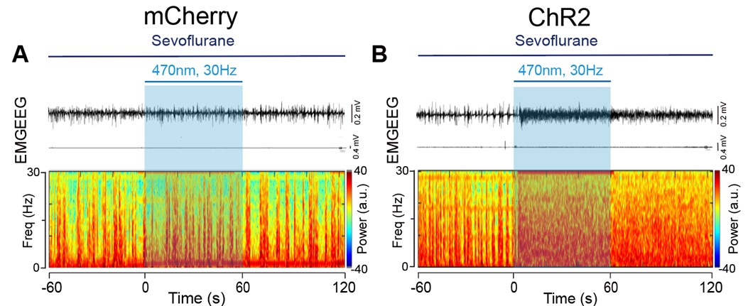
4) The spectrogram in Figure 2D has several frequency chirps that do not seem physiological.
Thank you for your comments. The frequency chips of the spectrogram during the During and Post 1 phase were caused by recording noises. To avoid confusion, we have deleted the spectrogram in Figure 2D.
5) The 3D plots in Figures 3G and H are not helpful. Thanks for the comment. We'd like to keep the 3D plots as they aid visual comparison of three different features of grooming, which complements other panels in Figure 3.
6) The spectrograms in Figures 5A and B are too small, while the spectra in Figures 5C and D are too large. Please invert this relationship, as it is interesting and important to see the details in the spectrograms. The same happens in Figure 6.
We adjusted the layout of the Figure 5 and Figure 6 as requested, please see below:
Author response image 6.
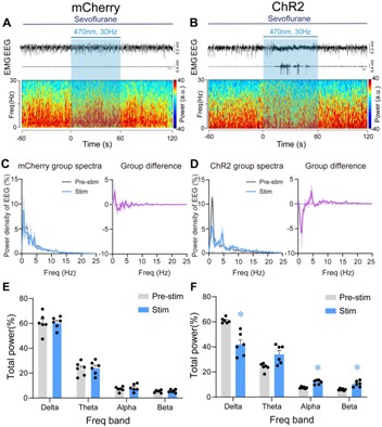
Author response image 7.
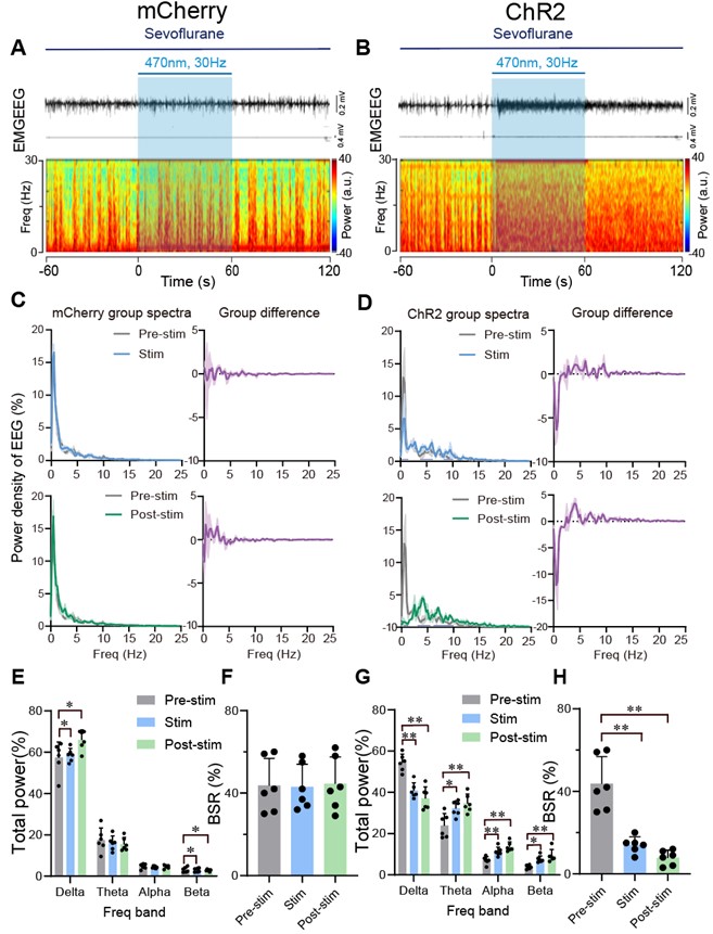
7) In Figure 6H, the authors compute the burst-suppression ratio during a period that seemingly has no bursts or suppressions (Figure 6B).
The burst-suppression ratio was computed from data with the minimum duration of burst and suppression periods set at 0.5 s. Sorry for the confusion. We added a new supplementary figure (Figure 6-figure supplement 8) displaying a 40-second EEG with a burst suppression period to better visualize the burst suppression.
Author response image 8.
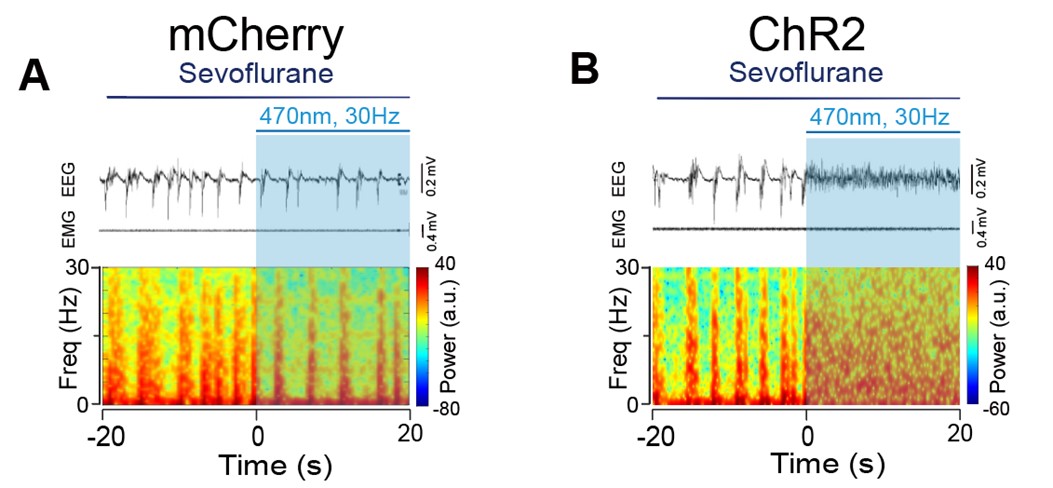
8) The data analyses are done in terms of p-values. They should be reported as confidence intervals so that any effect the authors wish to establish is measured along with its uncertainty.
Thank you for your valuable suggestions regarding our manuscript. We appreciate your thoughtful consideration of our work. We understand your concern but we would like to provide some justification for our choice of reporting p-values and explain why we believe they are appropriate for our study. First, the use of p-values for hypothesis testing and significance assessment is a common practice in our field. Many previous studies in our area of research also report results in terms of p-values. For example, Wei Xu11 published in 2020 suggested sevoflurane inhibits MPB neurons through postsynaptic GABAA-Rs and background potassium channels, Ao Y12 demonstrated that activation of the TH:LC-PVT projections is helpful in facilitating the transition from isoflurane anesthesia to an arousal state, using P-value as data analyses. By adhering to this convention, we ensure that our findings are consistent with the existing body of literature. This makes it easier for readers to compare and integrate our results with previous work. Secondly, while confidence intervals can provide a measure of effect size and uncertainty, p-values offer a concise way to communicate statistical significance. They help readers quickly assess whether an effect is statistically significant or not, which is often the primary concern when interpreting research findings. We hope that by providing these reasons for our choice of reporting p-values, we can address your concern while maintaining the integrity and consistency of our study. If you believe there are specific instances where reporting confidence intervals would be more informative, please feel free to highlight those, and we will consider your suggestion on a case-by-case basis.
References
Author response:
The following is the authors’ response to the previous reviews
Public Reviews:
Reviewer #1 (Public review):
(1) Authors' experimental designs have some caveats to definitely support their claims. Authors claimed that aged LT-HSCs have no myeloid-biased clone expansion using transplantation assays. In these experiments, authors used 10 HSCs and young mice as recipients. Given the huge expansion of old HSC by number and known heterogeneity in immunophenotypically defined HSC populations, it is questionable how 10 out of so many old HSCs (an average of 300,000 up to 500,000 cells per mouse; Mitchell et al., Nature Cell Biology, 2023) can faithfully represent old HSC population. The Hoxb5+ old HSC primary and secondary recipient mice data (Fig. 2C and D) support this concern. In addition, they only used young recipients. Considering the importance of inflammatory aged niche in the myeloid-biased lineage output, transplanting young vs old LT-HSCs into aged mice will complete the whole picture.
We sincerely appreciate your insightful comment regarding the existence of approximately 500,000 HSCs per mouse in older mice. To address this, we have conducted a statistical analysis to determine the appropriate sample size needed to estimate the characteristics of a population of 500,000 cells with a 95% confidence level and a ±5% margin of error. This calculation was performed using the finite population correction applied to Cochran’s formula.
For our calculations, we used a proportion of 50% (p = 0.5), as it has been reported that approximately 50% of HSCs are myeloid-biased1,2. The formula used is as follows:
N \= 500,000 (total population size)
Z = 1.96 (Z-score for a 95% confidence level)
p = 0.5 (expected proportion)
e \= 0.05 (margin of error)
Applying this formula, we determined that the required sample size is approximately 384 cells. This sample size ensures that the observed proportion in the sample will reflect the characteristics of the entire population. In our study, we have conducted functional experiments across Figures 2, 3, 5, 6, S3, and S6, with a total sample size of n = 126, which corresponds to over 1260 cells. While it would be ideal to analyze all 500,000 cells, this would necessitate the use of 50,000 recipient mice, which is not feasible. We believe that the number of cells analyzed is reasonable from a statistical standpoint.
References
(1) Dykstra, Brad et al. “Clonal analysis reveals multiple functional defects of aged murine hematopoietic stem cells.” The Journal of experimental medicine vol. 208,13 (2011): 2691-703. doi:10.1084/jem.20111490
(2) Beerman, Isabel et al. “Functionally distinct hematopoietic stem cells modulate hematopoietic lineage potential during aging by a mechanism of clonal expansion.” Proceedings of the National Academy of Sciences of the United States of America vol. 107,12 (2010): 5465-70. doi:10.1073/pnas.1000834107
(2) Authors' molecular data analyses need more rigor with unbiased approaches. They claimed that neither aged LT-HSCs nor aged ST-HSCs exhibited myeloid or lymphoid gene set enrichment but aged bulk HSCs, which are just a sum of LTHSCs and ST-HSCs by their gating scheme (Fig. 4A), showed the "tendency" of enrichment of myeloid-related genes based on the selected gene set (Fig. 4D). Although the proportion of ST-HSCs is reduced in bulk HSCs upon aging, since STHSCs do not exhibit lymphoid gene set enrichment based on their data, it is hard to understand how aged bulk HSCs have more myeloid gene set enrichment compared to young bulk HSCs. This bulk HSC data rather suggest that there could be a trend toward certain lineage bias (although not significant) in aged LT-HSCs or ST-HSCs. Authors need to verify the molecular lineage priming of LT-HSCs and ST-HSCs using another comprehensive dataset.
Thank you for your thoughtful feedback regarding the lack of myeloid or lymphoid gene set enrichment in aged LT-HSCs and aged ST-HSCs, despite the observed tendency for myeloid-related gene enrichment in aged bulk HSCs.
First, we acknowledge that the GSEA results vary among the different myeloid gene sets analyzed (Fig. 4, D–F; Fig. S4, C–D). Additionally, a comprehensive analysis of mouse HSC aging using multiple RNA-seq datasets reported that nearly 80% of differentially expressed genes show poor reproducibility across datasets[1]. These factors highlight the challenges of interpreting lineage bias in HSCs based solely on previously published transcriptomic data.
Given these points, we believe that emphasizing functional experimental results is more critical than incorporating an additional dataset to support our claim. In this regard, we have confirmed that young and aged LT-HSCs have similar differentiation capacity (Figure 3), while myeloid-biased hematopoiesis is observed in aged bulk HSCs (Figure S3). These findings are further corroborated by independent functional experiments. We sincerely appreciate your insightful comments.
Reference
(1) Flohr Svendsen, Arthur et al. “A comprehensive transcriptome signature of murine hematopoietic stem cell aging.” Blood vol. 138,6 (2021): 439-451. doi:10.1182/blood.2020009729
(3) Although authors could not find any molecular evidence for myeloid-biased hematopoiesis from old HSCs (either LT or ST), they argued that the ratio between LT-HSC and ST-HSC causes myeloid-biased hematopoiesis upon aging based on young HSC experiments (Fig. 6). However, old ST-HSC functional data showed that they barely contribute to blood production unlike young Hoxb5- HSCs (ST-HSC) in the transplantation setting (Fig. 2). Is there any evidence that in unperturbed native old hematopoiesis, old Hoxb5- HSCs (ST-HSC) still contribute to blood production?
If so, what are their lineage potential/output? Without this information, it is hard to argue that the different ratio causes myeloid-biased hematopoiesis in aging context.
Thank you for the insightful and important question. The post-transplant chimerism of ST-HSCs was low in Fig. 2, indicating that transplantation induced a short-term loss of hematopoietic potential due to hematopoietic stress per cell.
To reduce this stress, we increased the number of HSCs in transplantation setting. In Fig. S6, old LT-HSCs and old ST-HSCs were transplanted in a 50:50 or 20:80 ratio, respectively. As shown in Fig. S6.D, the 20:80 group, which had a higher proportion of old ST-HSCs, exhibited a statistically significant increase in the lymphoid percentage in the peripheral blood post-transplantation.
These findings suggest that old ST-HSCs contribute to blood production following transplantation.
Reviewer #2 (Public review):
While aspects of their work are fascinating and might have merit, several issues weaken the overall strength of the arguments and interpretation. Multiple experiments were done with a very low number of recipient mice, showed very large standard deviations, and had no statistically detectable difference between experimental groups. While the authors conclude that these experimental groups are not different, the displayed results seem too variable to conclude anything with certainty. The sensitivity of the performed experiments (e.g. Fig 3; Fig 6C, D) is too low to detect even reasonably strong differences between experimental groups and is thus inadequate to support the author's claims. This weakness of the study is not acknowledged in the text and is also not discussed. To support their conclusions the authors need to provide higher n-numbers and provide a detailed power analysis of the transplants in the methods section.
Response #2-1:
Thank you for your important remarks. The power analysis for this experiment shows that power = 0.319, suggesting that more number may be needed. On the other hand, our method for determining the sample size in Figure 3 is as follows:
(1) First, we checked whether myeloid biased change is detected in the bulk-HSC fraction (Figure S3). The results showed that the difference in myeloid output at 16 weeks after transplantation was statistically significant (young vs. aged = 7.2 ± 8.9 vs. 42.1 ± 35.5%, p = 0.01), even though n = 10.
(2) Next, myeloid biased HSCs have been reported to be a fraction with high selfrenewal ability (2004, Blood). If myeloid biased HSCs increase with aging, the increase in myeloid biased HSCs in LT-HSC fraction would be detected with higher sensitivity than in the bulk-HSC fraction used in Figure S3.
(3) However, there was no difference not only in p-values but also in the mean itself, young vs aged = 51.4±31.5% vs 47.4±39.0%, p = 0.82, even though n = 8 in Figure 3. Since there was no difference in the mean itself, it is highly likely that no difference will be detected even if n is further increased.
Regarding Figure 6, we obtained a statistically significant difference and consider the sample size to be sufficient. In addition, we have performed various functional experiments (Figures 2, 5, 6 and S6), and have obtained consistent results that expansion of myeloid biased HSCs does not occur with aging in Hoxb5+HSCs fraction. Based on the above, we conclude that the LT-HSC fraction does not differ in myeloid differentiation potential with aging.
As the authors attempt to challenge the current model of the age-associated expansion of myeloid-biased HSCs (which has been observed and reproduced by many different groups), ideally additional strong evidence in the form of single-cell transplants is provided.
Response #2-2:
Thank you for the comments. As the reviewer pointed out, we hope we could reconfirm our results using single-cell level technology in the future.
On the other hand, we have reported that the ratio of myeloid to lymphoid cells in the peripheral blood changes when the number of HSCs transplanted, or the number of supporting cells transplanted with HSCs, is varied[1-2]. Therefore, single-cell transplant data need to be interpreted very carefully to determine differentiation potential.
From this viewpoint, future experiments will combine the Hoxb5 reporter system with a lineage tracing system that can track HSCs at the single-cell level over time. This approach will investigate changes in the self-renewal capacity of individual HSCs and their subsequent differentiation into progenitor cells and peripheral blood cells. We have reflected this comment by adding the following sentences in the manuscript.
[P19, L451] “In contrast, our findings should be considered in light of some limitations. In this report, we primarily performed ten to twenty cell transplantation assays. Therefore, the current theory should be revalidated using single-cell technology with lineage tracing system[3-4]. This approach will investigate changes in the self-renewal capacity of individual HSCs and their subsequent differentiation into progenitor cells and peripheral blood cells.”
It is also unclear why the authors believe that the observed reduction of ST-HSCs relative to LT-HSCs explains the myeloid-biased phenotype observed in the peripheral blood. This point seems counterintuitive and requires further explanation.
Response #2-3:
Thank you for your comment. We apologize for the insufficient explanation. Our data, as shown in Figures 3 and 4, demonstrate that the differentiation potential of LT-HSCs remains unchanged with age. Therefore, rather than suggesting that an increase in LT-HSCs with a consistent differentiation capacity leads to myeloidbiased hematopoiesis, it seems more accurate to highlight that the relative decrease in the proportion of ST-HSCs, which remain in peripheral blood as lymphocytes, leads to a relative increase in myeloid cells in peripheral blood and thus causes myeloid-biased hematopoiesis.
However, if we focus on the increase in the ratio of LT-HSCs, it is also plausible to explain that “with aging, the proportion of LT-HSCs capable of long-term myeloid hematopoiesis increases. As a result, from 16 weeks after transplantation, the influence of LT-HSCs maintaining the long-term ability to produce myeloid cells becomes relatively more significant, leading to an increase in the ratio of myeloid cells in the peripheral blood and causing myeloid-biased hematopoiesis.”
Based on my understanding of the presented data, the authors argue that myeloidbiased HSCs do not exist, as
a) they detect no difference between young/aged HSCs after transplant (mind low nnumbers and large std!!!); b) myeloid progenitors downstream of HSCs only show minor or no changes in frequency and c) aged LT-HSCs do not outperform young LT-HSC in myeloid output LT-HSCs in competitive transplants (mind low n-numbers and large std!!!).
However, given the low n-numbers and high variance of the results, the argument seems weak and the presented data does not support the claims sufficiently. That the number of downstream progenitors does not change could be explained by other mechanisms, for instance, the frequently reported differentiation short-cuts of HSCs and/or changes in the microenvironment.
Response #2-4:
We appreciate the comments. As mentioned above, we will correct the manuscript regarding the sample size. Regarding the interpreting of the lack of increase in the percentage of myeloid progenitor cells in the bone marrow with age, it is instead possible that various confounding factors, such as differentiation shortcuts or changes in the microenvironment, are involved.
However, even when aged LT-HSCs and young LT-HSCs are transplanted into the same recipient mice, the timing of the appearance of different cell fractions in peripheral blood is similar (Figure 3 of this paper). Therefore, we have not obtained data suggesting that clear shortcuts exist in the differentiation process of aged HSCs into neutrophils or monocytes. Additionally, it is currently consensually accepted that myeloid cells, including neutrophils and monocytes, differentiate from GMPs[1]. Since there is no changes in the proportion of GMPs in the bone marrow with age, we concluded that the differentiation potential into myeloid cells remains consistent with aging.
"Then, we found that the myeloid lineage proportions from young and aged LT-HSCs were nearly comparable during the observation period after transplantation (Fig. 3, B and C)."
[Comment to the authors]: Given the large standard deviation and low n-numbers, the power of the analysis to detect differences between experimental groups is very low. Experimental groups with too large standard deviations (as displayed here) are difficult to interpret and might be inconclusive. The absence of clearly detectable differences between young and aged transplanted HSCs could thus simply be a false-negative result. The shown experimental results hence do not provide strong evidence for the author's interpretation of the data. The authors should add additional transplants and include a detailed power analysis to be able to detect differences between experimental groups with reasonable sensitivity.
Response #2-5:
Thank you for providing these insights. Regarding the sample size, we have addressed this in Response #2-1.
Line 293: "Based on these findings, we concluded that myeloid-biased hematopoiesis observed following transplantation of aged HSCs was caused by a relative decrease in ST-HSC in the bulk-HSC compartment in aged mice rather than the selective expansion of myeloid-biased HSC clones."
Couldn't that also be explained by an increase in myeloid-biased HSCs, as repeatedly reported and seen in the expansion of CD150+ HSCs? It is not intuitively clear why a reduction of ST-HSCs clones would lead to a myeloid bias. The author should try to explain more clearly where they believe the increased number of myeloid cells comes from. What is the source of myeloid cells if the authors believe they are not derived from the expanded population of myeloid-biased HSCs? t
Response #2-6:
Thank you for pointing this out. We apologize for the insufficient explanation. We will explain using Figure 8 from the paper.
First, our data show that LT-HSCs maintain their differentiation capacity with age, while ST-HSCs lose their self-renewal capacity earlier, so that only long-lived memory lymphocytes remain in the peripheral blood after the loss of selfrenewal capacity in ST-HSCs (Figure 8, upper panel). In mouse bone marrow, the proportion of LT-HSCs increases with age, while the proportion of ST-HSCs relatively decreases (Figure 8, lower panel and Figure S5).
Our data show that merely reproducing the ratio of LT-HSCs to ST-HSCs observed in aged mice using young LT-HSCs and ST-HSCs can replicate myeloidbiased hematopoiesis. This suggests that the increase in LT-HSC and the relative decrease in ST-HSC within the HSC compartment with aging are likely to contribute to myeloid-biased hematopoiesis.
As mentioned earlier, since the differentiation capacity of LT-HSCs remain unchaged with age, it seems more accurate to describe that the relative decrease in the proportion of ST-HSCs, which retain long-lived memory lymphocytes in peripheral blood, leads to a relative increase in myeloid cells in peripheral blood and thus causes myeloid-biased hematopoiesis.
However, focusing on the increase in the proportion of LT-HSCs, it is also possible to explain that “with aging, the proportion of LT-HSCs capable of long-term myeloid hematopoiesis increases. As a result, from 16 weeks after transplantation, the influence of LT-HSCs maintaining the long-term ability to produce myeloid cells becomes relatively more significant, leading to an increase in the ratio of myeloid cells in the peripheral blood and causing myeloid-biased hematopoiesis.”
Recommendations for the authors:
Reviewer #2 (Recommendations for the authors):
Summary:
Comment #2-1: While aspects of their work are fascinating and might have merit, several issues weaken the overall strength of the arguments and interpretation. Multiple experiments were done with a very low number of recipient mice, showed very large standard deviations, and had no statistically detectable difference between experimental groups. While the authors conclude that these experimental groups are not different, the displayed results seem too variable to conclude anything with certainty. The sensitivity of the performed experiments (e.g. Figure 3; Figure 6C, D) is too low to detect even reasonably strong differences between experimental groups and is thus inadequate to support the author's claims. This weakness of the study is not acknowledged in the text and is also not discussed. To support their conclusions the authors, need to provide higher n-numbers and provide a detailed power analysis of the transplants in the methods section.
Response #2-1
Thank you for your important remarks. The power analysis for this experiment shows that power = 0.319, suggesting that more number may be needed. On the other hand, our method for determining the sample size in Figure 3 is as follows:
(1) First, we checked whether myeloid biased change is detected in the bulk-HSC fraction (Figure S3). The results showed that the difference in myeloid output at 16 weeks after transplantation was statistically significant (young vs. aged = 7.2 {plus minus} 8.9 vs. 42.1 {plus minus} 35.5%, p = 0.01), even though n = 10.
(2) Next, myeloid biased HSCs have been reported to be a fraction with high selfrenewal ability (2004, Blood). If myeloid biased HSCs increase with aging, the increase in myeloid biased HSCs in LT-HSC fraction would be detected with higher sensitivity than in the bulk-HSC fraction used in Figure S3.
(3) However, there was no difference not only in p-values but also in the mean itself, young vs aged = 51.4{plus minus}31.5% vs 47.4{plus minus}39.0%, p = 0.82, even though n = 8 in Figure 3. Since there was no difference in the mean itself, it is highly likely that no difference will be detected even if n is further increased.
Regarding Figure 6, we obtained a statistically significant difference and consider the sample size to be sufficient. In addition, we have performed various functional experiments (Figures 2, 5, 6 and S6), and have obtained consistent results that expansion of myeloid-biased HSCs does not occur with aging in Hoxb5+HSCs fraction. Based on the above, we conclude that the LT-HSC fraction does not differ in myeloid differentiation potential with aging.
[Comment for authors]
Paradigm-shifting extraordinary claims require extraordinary data. Unfortunately, the authors do not provide additional data to further support their claims. Instead, the authors argue the following: Because they were able to find significant differences between experimental groups in some experiments, the absence of significant differences in the results of other experiments must be correct, too.
This logic is in my view flawed. Any assay/experiment with highly variable data has a very low sensitivity to detect significant differences between groups. If, as in this case, the variance is as large as the entire dynamic range of the readout, it becomes impossible to be able to detect any difference. In these cases, it is not surprising and actually expected that the mean of the group is located close to the center of the dynamic range as is the case here (center of dynamic range: 50%). In other words, this means that the experiments are simply not reproducible. It is absolutely critical to remember that any experiment and its associated statistical analysis has 3 (!!!) instead of 2 possible outcomes:
(1) There is a statistically significant difference
(2) There is no statistically significant difference
(3) The results of the experiment are inconclusive because the replicates are too variable and the results are not reproducible.
While most of us are inclined to think about outcomes (1) or (2), outcome (3) cannot be neglected. While it might be painful to accept, the only way to address concerns about data reproducibility is to provide additional data, improve reproducibility, and lower the power of the analysis to an acceptable level (e.g. able to detect difference of 5-10% between groups).
Without going into the technical details, the example graph from the link below illustrates that with a power 0.319 as stated by the authors, approx. 25 transplants, instead of 8, would be required.
Typically, however, a power of 0.8 is a reasonable value for any power analysis (although it's not a very strong power either). Even if we are optimistic and assume that there might be a reasonably large difference between experimental groups (in the example above P2 = 0.6, which is actually not that large) we can estimate that we would need over 10 transplants per group to say with confidence that two experimental groups likely do not differ. With smaller differences, these numbers increase quickly to 20+ transplants per group as can be seen in the example graph using an Alpha of 0.1 above.
Further reading can be found here and in many textbooks or other online resources: https://power-analysis.com/effect_size.htm https://tss.awf.poznan.pl/pdf-188978-110207? filename=Using%20power%20analysis%20to.pdf
Response:
Thank you for your feedback. We fully agree with the reviewer that paradigmshifting claims must be supported by equally robust data. It has been welldocumented that the frequency of myeloid-biased HSCs increases with age, with reports indicating that over 50% of the HSC compartment in aged mice consists of myeloid-biased HSCs[1,2]. Based on this, we believe that if aged LT-HSCs were substantially myeloid-biased, the difference should be readily detectable.
To further validate our findings, we showed the similar preliminary experiment. The resulting data are shown below (n = 8).
Author response image 1.
(A) Experimental design for competitive co-transplantation assay. Ten CD45.2<sup>+</sup> young LT-HSCs and ten CD45.2<sup>+</sup> aged LT-HSCs were transplanted with 2 × 10<sup>5</sup> CD45.1<sup>+</sup>/CD45.2<sup>+</sup> supporting cells into lethally irradiated CD45.1<sup>+</sup> recipient mice (n \= 8). (B) Lineage output of young or aged LT-HSCs at 4, 8, 12, 16 weeks after transplantation. Each bar represents an individual mouse. *P < 0.05. **P < 0.01.
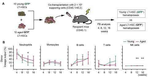
While a slight increase in myeloid-biased hematopoiesis was observed in the aged LT-HSC fraction, the difference was not statistically significant. These new results are presented alongside the original Figure 3, which was generated using a larger sample size (n = 16).
Author response image 2.
(A) Experimental design for competitive co-transplantation assay. Ten CD45.2<sup>+</sup> young LT-HSCs and ten CD45.2<sup>+</sup> aged LT-HSCs were transplanted with 2 × 10<sup>5</sup> CD45.1<sup>+</sup>/CD45.2<sup>+</sup> supporting cells into lethally irradiated CD45.1<sup>+</sup> recipient mice (n \= 16). (B) Lineage output of young or aged LT-HSCs at 4, 8, 12, 16 weeks after transplantation. Each bar represents an individual mouse.
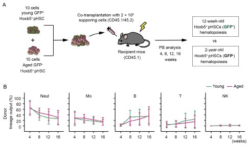
Consistent with the original data, aged LT-HSCs exhibited a lineage output that was nearly identical to that of young LT-HSCs. Nonetheless, as the reviewer rightly pointed out, we cannot completely exclude the possibility that subtle differences may exist but remain undetected. To address this, we have added the following sentence to the manuscript:
[P9, L200] “These findings unmistakably demonstrated that mixed/bulk-HSCs showed myeloid skewed hematopoiesis in PB with aging. In contrast, LT-HSCs maintained a consistent lineage output throughout life, although subtle differences between aged and young LT-HSCs may exist and cannot be entirely ruled out.”
References
(1) Dykstra, Brad et al. “Clonal analysis reveals multiple functional defects of aged murine hematopoietic stem cells.” The Journal of experimental medicine vol. 208,13 (2011): 2691-703. doi:10.1084/jem.20111490
(2) Beerman, Isabel et al. “Functionally distinct hematopoietic stem cells modulate hematopoietic lineage potential during aging by a mechanism of clonal expansion.” Proceedings of the National Academy of Sciences of the United States of America vol. 107,12 (2010): 5465-70. doi:10.1073/pnas.1000834107
Comment #2-3: It is also unclear why the authors believe that the observed reduction of STHSCs relative to LT-HSCs explains the myeloid-biased phenotype observed in the peripheral blood. This point seems counterintuitive and requires further explanation.
Response #2-3:
Thank you for your comment. We apologize for the insufficient explanation. Our data, as shown in Figures 3 and 4, demonstrate that the differentiation potential of LTHSCs remains unchanged with age. Therefore, rather than suggesting that an increase in LT-HSCs with a consistent differentiation capacity leads to myeloid biased hematopoiesis, it seems more accurate to highlight that the relative decrease in the proportion of ST-HSCs, which remain in peripheral blood as lymphocytes, leads to a relative increase in myeloid cells in peripheral blood and thus causes myeloid-biased hematopoiesis. However, if we focus on the increase in the ratio of LT-HSCs, it is also plausible to explain that "with aging, the proportion of LT-HSCs capable of long-term myeloid hematopoiesis increases. As a result, from 16 weeks after transplantation, the influence of LT-HSCs maintaining the long-term ability to produce myeloid cells becomes relatively more significant, leading to an increase in the ratio of myeloid cells in the peripheral blood and causing myeloid-biased hematopoiesis."
[Comment for authors]
While this interpretation of the data might make sense the shown data do not exclude alternative explanations. The authors do not exclude the possibility that LTHSCs expand with age and that this expansion in combination with an aging microenvironment drives myeloid bias. The authors should quantify the frequency [%] and absolute number of LT-HSCs and ST-HSCs in young vs. aged animals. Especially analyzing the abs. numbers of cells will be important to support their claims as % can be affected by changes in the frequency of other populations.
Thank you for your very important point. As this reviewer pointed out, we do not exclude the possibility that the combination of aged microenvironment drives myeloid bias. Additionally, we acknowledge that myeloid-biased hematopoiesis with age is a complex process likely influenced by multiple factors. We would like to discuss the mechanism mentioned as a future research direction. Thank you for the insightful feedback. Regarding the point about the absolute cell numbers mentioned in the latter half of the paragraph, we will address this in detail in our subsequent response (Response #2-4).
Comment #2-4: Based on my understanding of the presented data, the authors argue that myeloid-biased HSCs do not exist, as a) they detect no difference between young/aged HSCs after transplant (mind low n-numbers and large std!); b) myeloid progenitors downstream of HSCs only show minor or no changes in frequency and c) aged LT-HSCs do not outperform young LT-HSCs in myeloid output LTHSCs in competitive transplants (mind low n-numbers and large std!). However, given the low n-numbers and high variance of the results, the argument seems weak and the presented data does not support the claims sufficiently. That the number of downstream progenitors does not change could be explained by other mechanisms, for instance, the frequently reported differentiation short-cuts of HSCs and/or changes in the microenvironment.
Response #2-4:
We appreciate the comments. As mentioned above, we will correct the manuscript regarding the sample size. Regarding the interpreting of the lack of increase in the percentage of myeloid progenitor cells in the bone marrow with age, it is instead possible that various confounding factors, such as differentiation shortcuts or changes in the microenviroment, are involved. However, even when aged LT-HSCs and young LT-HSCs are transplanted into the same recipient mice, the timing of the appearance of different cell fractions in peripheral blood is similar (Figure 3 of this paper). Therefore, we have not obtained data suggesting that clear shortcuts exist in the differentiation process of aged HSCs into neutrophils or monocytes. Additionally, it is currently consensually accepted that myeloid cells, including neutrophils and monocytes, differentiate from GMPs1. Since there are no changes in the proportion of GMPs in the bone marrow with age, we concluded that the differentiation potential into myeloid cells remains consistent with aging.
Reference
(1) Akashi K and others, 'A Clonogenic Common Myeloid Progenitor That Gives Rise to All Myeloid Lineages', Nature, 404.6774 (2000), 193-97.
[Comment for authors]
As the relative frequency of cell population can be misleading, the authors should compare the absolute numbers of progenitors in young vs. aged mice to strengthen their argument. It would also be helpful to quantify the absolute numbers and relative frequencies in WT mice to exclude the possibility the HoxB5-trimcherry mouse model suffers from unexpected aging phenotypes and the hematopoietic system differs from wild-type animals.
Thank you for your valuable feedback. We understand the importance of comparing the absolute numbers of progenitors in young versus aged mice to provide a more accurate representation of the changes in cell populations.
Therefore, we quantified the absolute cell count of hematopoietic cells in the bone marrow using flow cytometry data.
Author response image 3.
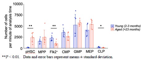
As previously reported, we observed a 10-fold increase in the number of pHSCs in aged mice compared to young mice. Additionally, our analysis revealed a statistically significant decrease in the number of Flk2+ progenitors and CLPs in aged mice. On the other hand, there was no statistically significant change in the number of myeloid progenitors between the two age groups. We appreciate the suggestion and hope that this additional information strengthens our argument and addresses your concerns.
Comment #2-5:
"Then, we found that the myeloid lineage proportions from young and aged LT-HSCs were nearly comparable during the observation period after transplantation (Figure 3, B and C)." Given the large standard deviation and low n-numbers, the power of the analysis to detect differences between experimental groups is very low. Experimental groups with too large standard deviations (as displayed here) are difficult to interpret and might be inconclusive. The absence of clearly detectable differences between young and aged transplanted HSCs could thus simply be a false-negative result. The shown experimental results hence do not provide strong evidence for the author's interpretation of the data. The authors should add additional transplants and include a detailed power analysis to be able to detect differences between experimental groups with reasonable sensitivity.
Response #2-5:
Thank you for providing these insights. Regarding the sample size, we have addressed this in Response #2-1.
[Comment for authors]
As explained in detail in the response to #2-1 the provided arguments are not convincing. As the authors pointed out, the power of these experiments is too low to make strong claims. If the author does not intend to provide new data, the language of the manuscript needs to be adjusted to reflect this weakness. A paragraph discussing the limitations of the study mentioning the limited power of the data should be included beyond the above-mentioned rather vague statement that the data should be validated (which is almost always necessary anyway).
Thank you for your valuable comment. We agree with the importance of discussing potential limitations in our experimental design. In response to the reviewer’s suggestion, we have revised the manuscript to include the following sentences:
[P19, L434] "In the co-transplantation assay shown in Figure 3, the myeloid lineage output derived from young and aged LT-HSCs was comparable (Young LT-HSC: 51.4 ± 31.5% vs. Aged LT-HSC: 47.4 ± 39.0%, p = 0.82). Although no significant difference was detected, the small sample size (n = 8) may limit the sensitivity of the assay to detect subtle myeloid-biased phenotypes."
This addition acknowledges the potential limitations of our analysis and highlights the need for further investigation with larger cohorts.
Comment #2-6:
Line 293: "Based on these findings, we concluded that myeloid biased hematopoiesis observed following transplantation of aged HSCs was caused by a relative decrease in ST-HSC in the bulk-HSC compartment in aged mice rather than the selective expansion of myeloid-biased HSC clones." Couldn't that also be explained by an increase in myeloid-biased HSCs, as repeatedly reported and seen in the expansion of CD150+ HSCs? It is not intuitively clear why a reduction of STHSCs clones would lead to a myeloid bias. The author should try to explain more clearly where they believe the increased number of myeloid cells comes from. What is the source of myeloid cells if the authors believe they are not derived from the expanded population of myeloid-biased HSCs?
Response #2-6:
Thank you for pointing this out. We apologize for the insufficient explanation. We will explain using attached Figure 8 from the paper. First, our data show that LT-HSCs maintain their differentiation capacity with age, while ST-HSCs lose their self-renewal capacity earlier, so that only long-lived memory lymphocytes remain in the peripheral blood after the loss of self-renewal capacity in ST-HSCs (Figure 8, upper panel). In mouse bone marrow, the proportion of LT-HSCs increases with age, while the proportion of STHSCs relatively decreases (Figure 8, lower panel and Figure S5).
Our data show that merely reproducing the ratio of LT-HSCs to ST-HSCs observed in aged mice using young LT-HSCs and ST-HSCs can replicate myeloid-biased hematopoiesis. This suggests that the increase in LT-HSC and the relative decrease in ST-HSC within the HSC compartment with aging are likely to contribute to myeloid-biased hematopoiesis.
As mentioned earlier, since the differentiation capacity of LT-HSCs remain unchanged with age, it seems more accurate to describe that the relative decrease in the proportion of STHSCs, which retain long-lived memory lymphocytes in peripheral blood, leading to a relative increase in myeloid cells in peripheral blood and thus causes myeloid-biased hematopoiesis. However, focusing on the increase in the proportion of LT-HSCs, it is also possible to explain that "with aging, the proportion of LT-HSCs capable of long-term myeloid hematopoiesis increases. As a result, from 16 weeks after transplantation, the influence of LT-HSCs maintaining the long-term ability to produce myeloid cells become relatively more significant, leading to an increase in the ratio of myeloid cells in the peripheral blood and causing myeloid biased hematopoiesis."
[Comment for authors]
While I can follow the logic of the argument, my concerns about the interpretation remain as I see discrepancies in other findings in the published literature. For instance, what the authors call ST-HSCs, differs from the classical functional definition of ST-HSCs. It is thus difficult to relate the described observations to previous reports. ST-HSCs typically can contribute significantly to multiple lineages for several weeks (see for example PMID: 29625072). It is somewhat surprising that the ST-HSC in this study don't show this potential and loose their potential much quicker.
The authors should thus provide a more comprehensive depth of immunophenotypic and molecular characterization to compare their LT-HSCs to ST-HSCs. For instance, are LT-HSCs CD41- HSCs? How do ST-HSCs differ in their surface marker expression from previously used definitions of ST-HSCs? A list of differentially expressed genes between young and old LT-HSCs and ST-HSCs should be done and will likely provide important insights into the molecular programs/markers (beyond the provided GO analysis, which seems superficial).
Thank you for your valuable feedback. As the reviewer noted, there are indeed multiple definitions of ST-HSCs. We appreciate the opportunity to clarify our definitions of ST-HSCs. We define ST-HSCs functionally, rather than by surface antigens, which we believe is the most classical and widely accepted definition [1]. In our study, we define long-term hematopoietic stem cells (LT-HSCs) as those HSCs that continue to contribute to hematopoiesis after a second transplantation and possess long-term self-renewal potential. Conversely, we define short-term hematopoietic stem cells (ST-HSCs) as those HSCs that do not contribute to hematopoiesis after a second transplantation and only exhibit self-renewal potential in the short term.
Next, in the paper referenced by the reviewer[2], the chimerism of each fraction of ST-HSCs also peaked at 4 weeks and then decreased to approximately 0.1% after 12 weeks post-transplantation. Author response image 5 illustrates our ST-HSC donor chimerism in Figure 2. We believe that data in the paper referenced by the reviewer2 is consistent with our own observations of the hematopoietic pattern following ST-HSC transplantation, indicating a characteristic loss of hematopoietic potential 4 weeks after the transplantation. Furthermore, as shown in Figures 2D and 2F, the fraction of ST-HSCs does not exhibit hematopoietic activity after the second transplantation. Therefore, we consider this fraction to be ST-HSCs.
Author response image 4.
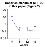
Additionally, the RNAseq data presented in Figures 4 and S4 revealed that the GSEA results vary among the different myeloid gene sets analyzed (Fig. 4, D–F; Fig. S4, C–D). Moreover, a comprehensive analysis of mouse HSC aging using multiple RNA-seq datasets reported that nearly 80% of differentially expressed genes show poor reproducibility across datasets[3]. From the above, while RNAseq data is indeed helpful, we believe that emphasizing functional experimental results is more critical than incorporating an additional dataset to support our claim. Thank you once again for your insightful feedback.
References
(1) Kiel, Mark J et al. “SLAM family receptors distinguish hematopoietic stem and progenitor cells and reveal endothelial niches for stem cells.” Cell vol. 121,7 (2005): 1109-21. doi:10.1016/j.cell.2005.05.026
(2) Yamamoto, Ryo et al. “Large-Scale Clonal Analysis Resolves Aging of the Mouse Hematopoietic Stem Cell Compartment.” Cell stem cell vol. 22,4 (2018): 600-607.e4. doi:10.1016/j.stem.2018.03.013
(3) Flohr Svendsen, Arthur et al. “A comprehensive transcriptome signature of murine hematopoietic stem cell aging.” Blood vol. 138,6 (2021): 439-451. doi:10.1182/blood.2020009729
Reviewer #3 (Public review):
Although the topic is appropriate and the new model provides a new way to think about lineage-biased output observed in multiple hematopoietic contexts, some of the experimental design choices, as well as some of the conclusions drawn from the results could be substantially improved. Also, they do not propose any potential mechanism to explain this process, which reduces the potential impact and novelty of the study.
The authors have satisfactorily replied to some of my comments. However, there are multiple key aspects that still remain unresolved.
Reviewer #3 (Recommendations for the authors):
Comment #3-1,2:
Although the additional details are much appreciated the core of my original comments remains unanswered. There are still no details about the irradiation dose for each particular experiment. Is any transplant performed using a 9.1 Gy dose? If yes, please indicate it in text or figure legend. If not, please remove this number from the corresponding method section.
Again, 9.5 Gy (split in two doses) is commonly reported as sublethal. The fact that the authors used a methodology that deviates from the "standard" for the field makes difficult to put these results in context with previous studies. It is not possible to know if the direct and indirect effects of this conditioning method in the hematopoietic system have any consequences in the presented results.
Thank you for your clarification. We confirm that none of the transplantation experiments described were performed using a 9.1 Gy irradiation dose. We have therefore removed the mention of "9.1 Gy" from the relevant section of the Materials and Methods. We appreciate helpful suggestion to improve the clarity of the manuscript.
[P22, L493] “12-24 hours prior to transplantation, C57BL/6-Ly5.1 mice, or aged C57BL/6J recipient mice were lethally irradiated with single doses of 8.7 Gy.”
Regarding the reviewer’s concern about the radiation dose used in our experiments, we will address this point in more detail in our subsequent response (see Response #3-4).
Comment #3-4(Original): When representing the contribution to PB from transplanted cells, the authors show the % of each lineage within the donor-derived cells (Figures 3B-C, 5B, 6B-D, 7C-E, and S3 B-C). To have a better picture of total donor contribution, total PB and BM chimerism should be included for each transplantation assay. Also, for Figures 2C-D and Figures S2A-B, do the graphs represent 100% of the PB cells? Are there any radioresistant cells?
Response #3-4 (Original): Thank you for highlighting this point. Indeed, donor contribution to total peripheral blood (PB) is important information. We have included the donor contribution data for each figure above mentioned.
In Figure 2C-D and Figure S2A-B, the percentage of donor chimerism in PB was defined as the percentage of CD45.1-CD45.2+ cells among total CD45.1-CD45.2+ and CD45.1+CD45.2+ cells as described in method section.
Comment for our #3-4 response:
Thanks for sharing these data. These graphs should be included in their corresponding figures along with donor contribution to BM.
Regarding Figure2 C-D, as currently shown, the graphs only account for CD45.1CD45.2+ (donor-derived) and CD45.1+CD45.2+ (supporting-derived). What is the percentage of CD45.1+CD45.2- (recipient-derived)? Since the irradiation regiment is atypical, including this information would help to know more about the effects of this conditioning method.
Thank you for your insightful comment regarding Figure 2C-D. To address the concern that the reviewer pointed out, we provide the kinetics of the percentage of CD45.1+CD45.2- (recipient-derived) in Author response image 7.
Author response image 5.
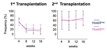
As the reviewer pointed out, we observed the persistence of recipient-derived cells, particularly in the secondary transplant. As noted, this suggests that our conditioning regimen may have been suboptimal. In response, we will include the donor chimerism analysis in the total cells and add the following statement in the study limitations section to acknowledge this point:
[P19, L439] “Additionally, in this study, we purified LT-HSCs using the Hoxb5 reporter system and employed a moderate conditioning regimen (8.7 Gy). To have a better picture of total donor contribution, total PB chimerism are presented in Figure S7 and we cannot exclude the possibility that these factors may have influenced the results. Therefore, it would be ideal to validate our findings using alternative LT-HSC markers and different conditioning regimens.”
Comment #3-5: For BM progenitor frequencies, the authors present the data as the frequency of cKit+ cells. This normalization might be misleading as changes in the proportion of cKit+ between the different experimental conditions could mask differences in these BM subpopulations. Representing this data as the frequency of BM single cells or as absolute numbers (e.g., per femur) would be valuable.
Response #3-5:
We appreciate the reviewer's comment on this point.
Firstly, as shown in Supplemental Figures S1B and S1C, we analyze the upstream (HSC, MPP, Flk2+) and downstream (CLP, MEP, CMP, GMP) fractions in different panels. Therefore, normalization is required to assess the differentiation of HSCs from upstream to downstream.
Additionally, the reason for normalizing by c-Kit+ is that the bone marrow analysis was performed after enrichment using the Anti-c-Kit antibody for both upstream and downstream fractions. Based on this, we calculated the progenitor populations as a frequency within the c-Kit positive cells. Next, the results of normalizing the whole bone marrow cells (live cells) are shown below.
Author response image 6.
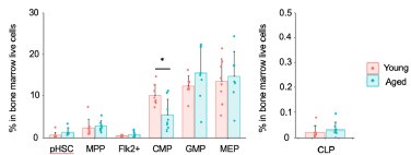
Similar to the results of normalizing c-Kit+ cells, myeloid progenitors remained unchanged, including a statistically significant decrease in CMP in aged mice. Additionally, there were no significant differences in CLP. In conclusion, similar results were obtained between the normalization with c-Kit and the normalization with whole bone marrow cells (live cells).
However, as the reviewer pointed out, it is necessary to explain the reason for normalization with c-Kit. Therefore, we will add the following description.
[P21, L502] For the combined analysis of the upstream (HSC, MPP, Flk2+) and downstream (CLP, MEP, CMP, GMP) fractions in Figures 1B, we normalized by cKit+ cells because we performed a c-Kit enrichment for the bone marrow analysis.
Comment for our #3-5 response:
I understand that normalization is necessary to compare across different BM populations. However, the best way would be to normalize to single cells. As I mentioned in my original comment, normalizing to cKit+ cells could be misleading, as the proportion of cKit+ cells could be different across the experimental conditions. Further, enriching for cKit+ cells when analyzing BM subpopulation frequencies could introduce similar potential errors. The enrichment would depend on the level of expression of cKit for each of these population, what would alter the final quantification. Indeed, CLP are typically defined as cKit-med/low. Thus, cKit enrichment would not be a great method to analyze the frequency of these cells.
The graph in the authors' response to my comment, show similar trend to what is represented Figure 1B for some populations. However, there are multiple statistically significant changes that disappear in this new version. This supports my original concern and, in consequence, I would encourage to represent this data as the frequency of BM single cells or as absolute numbers (e.g., per femur).
Thank you for your thoughtful follow-up comment. In response to the reviewer’s suggestion, we will represent the data as the frequency among total BM single cells. These revised graphs have been incorporated into the updated Figure 7F and corresponding figure legend have been revised accordingly to accurately reflect these representations. We appreciate your valuable input, which has helped us improve the clarity and rigor of our data presentation.
Comment #3-6: Regarding Figure 1B, the authors argue that if myeloid-biased HSC clones increase with age, they should see increased frequency of all components of the myeloid differentiation pathway (CMP, GMP, MEP). This would imply that their results (no changes or reduction in these myeloid subpopulations) suggest the absence of myeloid-biased HSC clones expansion with age. This reviewer believes that differentiation dynamics within the hematopoietic hierarchy can be more complex than a cascade of sequential and compartmentalized events (e.g., accelerated differentiation at the CMP level could cause exhaustion of this compartment and explain its reduction with age and why GMP and MEP are unchanged) and these conclusions should be considered more carefully.
Response #3-6:
We wish to thank the reviewer for this comment. We agree with that the differentiation pathway may not be a cascade of sequential events but could be influenced by various factors such as extrinsic factors.
In Figure 1B, we hypothesized that there may be other mechanisms causing myeloid-biased hematopoiesis besides the age-related increase in myeloid-biased HSCs, given that the percentage of myeloid progenitor cells in the bone marrow did not change with age. However, we do not discuss the presence or absence of myeloid-biased HSCs based on the data in Figure 1B.
Our newly proposed theories—that the differentiation capacity of LT-HSCs remains unchanged with age and that age-related myeloid-biased hematopoiesis is due to changes in the ratio of LT-HSCs to ST-HSCs—are based on functional experiment results. As the reviewer pointed out, to discuss the presence or absence of myeloid-biased HSCs based on the data in Figure 1B, it is necessary to apply a system that can track HSC differentiation at single-cell level. The technology would clarify changes in the self-renewal capacity of individual HSCs and their differentiation into progenitor cells and peripheral blood cells. The authors believe that those single-cell technologies will be beneficial in understanding the differentiation of HSCs. Based on the above, the following statement has been added to the text.
[P19, L440] In contrast, our findings should be considered in light of some limitations. In this report, we primarily performed ten to twenty cell transplantation assays. Therefore, the current theory should be revalidated using single-cell technology with lineage tracing system1-2. This approach will investigate changes in the self-renewal capacity of individual HSCs and their subsequent differentiation into progenitor cells and peripheral blood cells.
Comment for our #3-6 response:
Thanks for the response. My original comments referred to the statement "On the other hand, in contrast to what we anticipated, the frequency of GMP was stable, and the percentage of CMP actually decreased significantly with age, defying our prediction that the frequency of components of the myeloid differentiation pathway, such as CMP, GMP, and MEP would increase in aged mice if myeloid-biased HSC clones increase with age (Fig. 1 B)" (lines #129-133). Again, the absence of an increase in CMP, GMP and MEP with age does not mean the absence of and increase in myeloid-biased HSC clones. This statement should be considered more carefully.
Thank you for the insightful comment. We agree that the absence of an increase in CMP, GMP and MEP with age does not mean the absence of an increase in myeloid-biased HSC clones. In our revised manuscript, we have refined the statement to acknowledge this nuance more clearly. The updated text now reads as follows:
P6, L129] On the other hand, in contrast to what we anticipated, the frequency of GMP was stable, and the percentage of CMP actually decreased significantly with age, defying our prediction that the frequency of components of the myeloid differentiation pathway, such as CMP, GMP, and MEP may increase in aged mice, if myeloid-biased HSC clones increase with age.
Comment #3-7: Within the few recipients showing good donor engraftment in Figure 2C, there is a big proportion of T cells that are "amplified" upon secondary transplantation (Figure 2D). Is this expected?
Response #3-7:
We wish to express our deep appreciation to the reviewer for insightful comment on this point. As the reviewers pointed out, in Figure 2D, a few recipients show a very high percentage of T cells. The authors had the same question and considered this phenomenon as follows:
(1) One reason for the very high percentage of T cells is that we used 1 x 10⁷ whole bone marrow cells in the secondary transplantation. Consequently, the donor cells in the secondary transplantation contained more T-cell progenitor cells, leading to a greater increase in T cells compared to the primary transplantation.
(2) We also consider that this phenomenon may be influenced by the reduced selfrenewal capacity of aged LT-HSCs, resulting in decreased sustained production of myeloid cells in the secondary recipient mice. As a result, long-lived memorytype lymphocytes may preferentially remain in the peripheral blood, increasing the percentage of T cells in the secondary recipient mice.
We have discussed our hypothesis regarding this interesting phenomenon. To further clarify the characteristics of the increased T-cell count in the secondary recipient mice, we will analyze TCR clonality and diversity in the future.
Comment for our #3-7 response:
Thanks for the potential explanations to my question. This fact is not commonly reported in previous transplantation studies using aged HSCs. Could Hoxb5 label fraction of HSCs that is lymphoid/T-cell biased upon secondary transplantation? The number of recipients with high frequency of lymphoid cells in the peripheral blood (even from young mice) is remarkable.
Response:
Thank you for your insightful suggestion. Based on this comment, we calculated the percentage of lymphoid cells in the donor fraction at 16 weeks following the secondary transplantation, which was 56.1 ± 25.8% (L/M = 1.27). According to the Müller-Sieburg criteria, lymphoid-biased hematopoiesis is defined as having an L/M ratio greater than 10.
Given our findings, we concluded that the Hoxb5-labeled fraction does not specifically indicate lymphoid-biased hematopoiesis. We sincerely appreciate the valuable input, which helped us to further clarify the interpretation of our results.
Comment #3-8: Do the authors have any explanation for the high level of variabilitywithin the recipients of Hoxb5+ cells in Figure 2C?
Response #3-8:
We appreciate the reviewer's comment on this point. As noted in our previous report, transplantation of a sufficient number of HSCs results in stable donor chimerism, whereas a small number of HSCs leads to increased variability in donor chimerism1. Additionally, other studies have observed high variability when fewer than 10 HSCs are transplanted2-3. Based on this evidence, we consider that the transplantation of a small number of cells (10 cells) is the primary cause of the high level of variability observed.
Comment for our #3-8 response:
I agree that transplanting low number of HSC increases the mouse-to-mouse variability. For that reason, a larger cohort of recipients for this kind of experiment would be ideal.
Response:
Thank you for the insightful comment. We agree that a larger cohort of recipients would be ideal for this type of experiment. In Figure 2, the difference between Hoxb5<suup>+</sup> and Hoxb5⁻ cells are robust, allowing for a clear statistical distinction despite the cohort size. However, we also recognize that a larger cohort would be necessary to detect more subtle differences, particularly in Figure 3. In response, we have added the following statement to the main text to acknowledge this limitation.
P9, L200] These findings unmistakably demonstrated that mixed/bulk-HSCs showed myeloid skewed hematopoiesis in PB with aging. In contrast, LT-HSCs maintained a consistent lineage output throughout life, although subtle differences between aged and young LT-HSCs may exist and cannot be entirely ruled out.
Comment #3-10: Is Figure 2G considering all primary recipients or only the ones that were used for secondary transplants? The second option would be a fairer comparison.
Response #3-10:
We appreciate the reviewer's comment on this point. We considered all primary recipients in Figure 2G to ensure a fair comparison, given the influence of various factors such as the radiosensitivity of individual recipient mice[1]. Comparing only the primary recipients used in the secondary transplantation would result in n = 3 (primary recipient) vs. n = 12 (secondary recipient). Including all primary recipients yields n = 11 vs. n = 12, providing a more balanced comparison. Therefore, we analyzed all primary recipient mice to ensure the reliability of our results.
Comment for our #3-10 response:
I respectfully disagree. Secondary recipients are derived from only 3 of the primary recipients. Therefore, the BM composition is determined by the composition of their donors. Including primary recipients that are not transplanted into secondary recipients for is not the fairest comparison for this analysis.
Thank you for your comment and for highlighting this important issue. We acknowledge the concern that including primary recipients that are not transplanted into secondary recipients is not the fairest comparison for this analysis. In response, we have reanalyzed the data using only the primary recipients whose bone marrow was actually transplanted into secondary recipients.
Author response image 7.
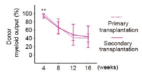
Importantly, the reanalysis confirmed that the kinetics of myeloid cell proportions in peripheral blood were consistent between primary and secondary transplant recipients. We sincerely appreciate your thoughtful feedback, which has helped us improve the clarity.
Comment #3-11: When discussing the transcriptional profile of young and aged HSCs, the authors claim that genes linked to myeloid differentiation remain unchanged in the LT-HSC fraction while there are significant changes in the STHSCs. However, 2 out of the 4 genes shown in Figure S4B show ratios higher than 1 in LT-HSCs.
Response #3-11:
Thank you for highlighting this important point. As the reviewer pointed out, when we analyze the expression of myeloid-related genes, some genes are elevated in aged LT-HSCs compared to young LT-HSCs. However, the GSEA analysis using myeloid-related gene sets, which include several hundred genes, shows no significant difference between young and aged LT-HSCs (see Figure S4C in this paper). Furthermore, functional experiments using the co-transplantation system show no difference in differentiation capacity between young and aged LT-HSCs (see Figure 3 in this paper). Based on these results, we conclude that LT-HSCs do not exhibit any change in differentiation capacity with aging.
Comment for our #3-11 response:
The authors used the data in Figure S4 to claim that "myeloid genes were tended to be enriched in aged bulk-HSCs but not in aged LT-HSCs compared to their respective controls" (this is the title of the figure; line # 1326). This is based on an increase in gene expression of CD150, vWF, Selp, Itgb3 in aged cells compared to young cells (Figure S4B). However, an increase in Selp and Itgb3 is also observed for LT-HSCs (lower magnitude, but still and increase).
Also, regarding the GSEA, the only term showing statistical significance in bulk HSCs is "Myeloid gene set", which does not reach significance in LT-HSCs, but present a trend for enrichment (q = 0.077). None of the terms in shown in this panel present statistical significance in ST-HSCs.
Thank you for your valuable point. As the reviewer noted, the current title may cause confusion. Therefore, we propose changing it to the following:
[P52, L1331] “Figure S4. Compared to their respective young controls, aged bulk-HSCs exhibit greater enrichment of myeloid gene expression than aged LT-HSCs”
Author response:
The following is the authors’ response to the previous reviews.
Public Reviews:
Reviewer #1 (Public review):
Summary:
The authors aim to assess the effect of salt stress on root:shoot ratio, identify the underlying genetic mechanisms, and evaluate their contribution to salt tolerance. To this end, the authors systematically quantified natural variations in salt-induced changes in root:shoot ratio. This innovative approach considers the coordination of root and shoot growth rather than exploring biomass and the development of each organ separately. Using this approach, the authors identified a gene cluster encoding eight paralog genes with a domain-of-unknown-function 247 (DUF247), with the majority of SNPs clustering into SR3G (At3g50160). In the manuscript, the authors utilized an integrative approach that includes genomic, genetic, evolutionary, histological, and physiological assays to functionally assess the contribution of their genes of interest to salt tolerance and root development.
Comments on revisions:
As the authors correctly noted, variations across samples, genotypes, or experiments make achieving statistical significance challenging. Should the authors choose to emphasize trends across experiments to draw biological conclusions, careful revisions of the text, including titles and figure legends, will be necessary to address some of the inconsistencies between figures (see examples below). However, I would caution that this approach may dilute the overall impact of the work on SR3G function and regulation. Therefore, I strongly recommend pursuing additional experimental evidence wherever possible to strengthen the conclusions.
(1) Given the phenotypic differences shown in Figures S17A-B, 10A-C, and 6A, the statement that "SR3G does not play a role in plant development under non-stress conditions" (lines 680-681) requires revision to better reflect the observed data.
Thank you to the reviewer for the comment. We appreciate the acknowledgment that variations among experiments are inherent to biological studies. Figures 6A and S17 represent the same experiment, which initially indicated a phenotype for the sr3g mutant under salt stress. To ensure that growth changes were specifically normalized for stress conditions, we calculated the Stress Tolerance Index (Fig. 6B). In Figure 10, we repeated the experiment including all five genotypes, which supported our original observation that the sr3g mutant exhibited a trend toward reduced lateral root number under 75 mM NaCl compared to Col-0, although this difference was not significant (Fig. 10B). Additionally, we confirmed that the wrky75 mutant showed a significant reduction in main root growth under salt stress compared to Col-0, consistent with findings reported in The Plant Cell by Lu et al. 2023. For both main root length and lateral root number, we demonstrated that the double mutants of wrky75/sr3g displayed growth comparable to wild-type Col-0. This result suggests that the sr3g mutation compensates for the salt sensitivity of the wrky75 mutant.
We completely agree with the reviewer that there is a variation in our results regarding the sr3g phenotype under control conditions, as presented in Fig. 6A/Fig. S17 and Fig. 10A-C. In Fig. 6A/Fig. S17, we did not observe any consistent trends in main root or lateral root length for the sr3g mutant compared to Col-0 under control conditions. However, in Fig. 10A-C, we observed a significant reduction in main root length, lateral root number, and lateral root length for the sr3g mutant under control conditions. We believe this may align with SR3G’s role as a negative regulator of salt stress responses. While loss of this gene benefits plants in coping with salt stress, it might negatively impact overall plant growth under non-stress conditions. This interpretation is further supported by our findings on the root suberization pattern in sr3g mutants under control conditions (Fig. 8B), where increased suberization in root sections 1 to 3, compared to Col-0, could inhibit root growth. While SR3G's role in overall plant fitness is intriguing, it is beyond the scope of this study. We cannot rule out the possibility that SR3G contributes positively to plant growth, particularly root growth. That said, we observed no differences in shoot growth between Col-0 and the sr3g mutant under control conditions (Fig. 7). Additionally, we calculated the Stress Tolerance Index for all aspects of root growth shown in Fig. 10 and presented it in Fig. S25.
To address the reviewer request on rephrasing the lines 680-681 from"SR3G does not play a role in plant development under non-stress conditions" (lines 680-681) statement, this statement is found in lines 652-653 and corresponds to Fig. 7, where we evaluated rosette growth in the WT and sr3g mutant under both control and salt stress conditions. We did not observe any significant differences or even trends between the two genotypes under control conditions, confirming the accuracy of the statement. To clarify further, we have added “SR3G does not play a role in rosette growth and development under non-stress conditions”.
(2) I agree with the authors that detecting expression differences in lowly expressed genes can be challenging. However, as demonstrated in the reference provided (Lu et al., 2023), a significant reduction in WRKY75 expression is observed in T-DNA insertion mutant alleles of WRKY75. In contrast, Fig. 9B in the current manuscript shows no reduction in WRKY75 expression in the two mutant alleles selected by the authors, which suggests that these alleles cannot be classified as loss-of-function mutants (line 745). Additionally, the authors note that the wrky75 mutant exhibits reduced main root length under salt stress, consistent with the phenotype reported by Lu et al. (2023). However, other phenotypic discrepancies exist between the two studies. For example, 1) Lu et al. (2023) report that w¬rky75 root length is comparable to WT under control conditions, whereas the current manuscript shows that wrky75 root growth is significantly lower than WT; 2) under salt stress, Lu et al. (2023) show that wrky75 accumulates higher levels of Na+, whereas the current study finds Na+ levels in wrky75 indistinguishable from WT. To confirm the loss of WRKY75 function in these T-DNA insertion alleles the authors should provide additional evidence (e.g., Western blot analysis).
We sincerely appreciate the reviewer acknowledging the challenge of detecting expression differences in lowly expressed genes, such as transcription factors. Transcription factors are typically expressed at lower levels compared to structural or enzymatic proteins, as they function as regulators where small quantities can have substantial effects on downstream gene expression.
That said, we respectfully disagree with the reviewer’s interpretation that there is no reduction in WRKY75 expression in the two mutant lines tested in Fig. 9C. Among the two independent alleles examined, wrky75-3 showed a clear reduction in expression compared to WT Col-0 under both control and salt stress conditions. Using the Tukey test to compare all groups, we observed distinct changes in the assigned significance letters for each case:
Col/root/control (cd) vs wrky75-3/root/control (cd): Although the same significance letter was assigned, we still observed a clear reduction in WRKY75 transcript abundance. More importantly, the variation in expression is notably lower compared to Col-0.
Col/shoot/control (bcd) vs wrky75-3/shoot/control (a): This is significant reduction compared to Col
Col/root/salt (cd) vs wrky75-3/root/salt (bcd): Once again, the reduction in WRKY75 transcript levels corresponds to changes in the assigned significance letters.
Col/shoot/salt (bc) vs wrky75-3/shoot/salt (ab): Once again, the reduction in WRKY75 transcript levels corresponds to changes in the assigned significance letters.
To address the reviewer’s comment regarding the significant reduction in WRKY75 expression observed in T-DNA insertion mutant alleles of WRKY75 in the reference by Lu et al., 2023, we would like to draw the reviewer’s attention to the following points:
a) Different alleles: The authors in The Plant Cell used different alleles than those used in our study, with one of their alleles targeting regions upstream of the WRKY75 gene. While we identified one of their described alleles (WRKY75-1, SALK_101367) on the T-DNA express website, which targets upstream of WRKY75, the other allele (wrky75-25) appears to have been generated through a different mechanism (possibly an RNAi line) that is not defined in the Plant Cell paper and does not appear on the T-DNA express website. The authors mentioned they have received these seeds as gifts from other labs in the acknowledgement ”We thank Prof. Hongwei Guo (Southern University of Science and Technology, China) and Prof. Diqiu Yu (Yunnan University, China) for kindly providing the WRKY75<sub>pro</sub>:GUS, 35S<sub>pro</sub>:WRKY75-GFP, wrky75-1, and wrky75-25 seeds. We thank Man-cang Zhang (Electrophysiology platform, Henan University) for performing the NMT experiment”.
However, in our study, we selected two different T-DNAs that target the coding regions. While this may explain slight differences in the observed responses, both studies independently link WRKY75 to salt stress, regardless of the alleles used. For your reference, we have included a screenshot of the different alleles used.
Author response image 1.
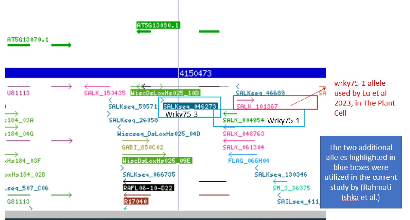
b) Different developmental stages: They measured WRKY75 expression in 5-day-old seedlings. In our experiment, we used seedlings grown on 1/2x MS for 4 days, followed by transfer to treatment plates with or without 75 mM NaCl for one week. As a result, we analyzed older plants (12 days old) for gene expression analysis. Despite the difference in developmental stage, we were still able to observe a reduction in gene expression.
c) Different tissues: The authors of The Plant Cell used whole seedlings for gene expression analysis, whereas we separated the roots and shoots and measured gene expression in each tissue type individually. This approach is logical, as WRKY75 is a root cell-specific transcription factor with higher expression in the roots compared to the shoots, as demonstrated in our analysis (Fig. 9C).
Based on the reasoning above, we did work with loss-of-function mutants of WRKY75, particularly wrky75-3. To more accurately reflect the nature of the mutation, we have changed the term "loss-of-function" to "knock-down" in line 717.
The reviewer mentioned phenotypic discrepancies between the two studies. We agree that there are some differences, particularly in the magnitude of responses or expression levels. However, despite variations in the alleles used, developmental stages, and tissue types, both studies reached the same conclusion: WRKY75 is involved in the salt stress response and acts as a positive regulator. We have discussed the differences between our study and The Plant Cell in the section above, summarizing them into three main points: different alleles, different developmental stages, and different tissue types.
To address the reviewer’s comment regarding "Lu et al. (2023) report that wrky75 root length is comparable to WT under control conditions, whereas the current manuscript shows that wrky75 root growth is significantly lower than WT": We evaluated root growth differently than The Plant Cell study. In The Plant Cell (Fig. 5, H-J), root elongation was measured in 10-day-old plants with a single time point measurement. They transferred five-day-old wild-type, wrky75-1, wrky75-25, and WRKY75-OE plants to 1/2× MS medium supplemented with 0 mM or 125 mM NaCl for further growth and photographed them 5 days after transfer. In contrast, our study used 4-day-old seedlings, which were transferred to 1/2 MS with or without 0, 75, or 125 mM salt for additional growth (9 days). Rather than measuring root growth only at the end, we scanned the roots every other day, up to five times, to assess root growth rates. Essentially, the precision of our method is higher as we captured growth changes throughout the developmental process, compared to the approach used in The Plant Cell. We do not underestimate the significance of the work conducted by other colleagues in the field, but we also recognize that each laboratory has its own approach and specific practices. This variation in experimental setup is intrinsic to biology, and we believe it is important to study biological phenomena in different ways. Especially as the common or contrasting conclusions reached by different studies, performed by different labs and using different experimental setups are shedding more light on reproducibility and gene contribution across different conditions, which is intrinsic to phenotypic plasticity, and GxE interactions.
The Plant Cell used a very high salt concentration, starting at 125 mM, while we were more cautious in our approach, as such a high concentration can inhibit and obscure more subtle phenotypic changes.
To address the reviewer’s comment on "Lu et al. (2023) show that wrky75 accumulates higher levels of Na+, whereas the current study finds Na+ levels in wrky75 indistinguishable from WT," we would like to highlight the differences in the methodologies used in both studies. The Plant Cell measured Na+ accumulation in the wrky75 mutant using xylem sap (Supplemental Figure S10), which appears to be a convenient and practical approach in their laboratory. In their experiment, wild-type and wrky75 mutant plants were grown in soil for 3 weeks, watered with either a mock solution or 100 mM NaCl solution for 1 day, and then xylem sap was collected for Na+ content analysis. In contrast, our study employed a different method to measure Na+ and K+ ion content, using Inductively Coupled Plasma Atomic Emission Spectroscopy (ICP-AES) for root and shoot Na+ and K+ measurements. Additionally, we collected samples after two weeks on treatment plates and focused on the Na+/K+ ratio, which we consider more relevant than net Na+ or K+ levels, as the ratio of these ions is a critical determinant of plant salt tolerance. With this in mind, we observed a considerable non-significant increase in the Na+/K+ ratio in the shoots of the wrky75-3 mutant (assigned Tukey’s letter c) compared to the Col-0 WT (assigned Tukey’s letters abc) under 125 mM salt, suggesting that this mutant is salt-sensitive. Importantly, the Na+/K+ ratio in the double wrky75/sr3g mutants was reduced to the WT level under the same salt conditions, further indicating that the salt sensitivity of wrky75 is mitigated by the sr3g mutation.
Based on the reasons mentioned above, we believe that conducting additional experiments, such as Western blot analysis, is unnecessary and would not contribute new insights or alter the context of our findings.
Reviewer #2 (Public review):
Summary:
Salt stress is a significant and growing concern for agriculture in some parts of the world. While the effects of sodium excess have been studied in Arabidopsis and (many) crop species, most studies have focused on Na uptake, toxicity and overall effects on yield, rather than on developmental responses to excess Na, per se. The work by Ishka and colleagues aims to fill this gap.
Working from an existing dataset that exposed a diverse panel of A. thaliana accessions to control, moderate, and severe salt stress, the authors identify candidate loci associated with altering the root:shoot ratio under salt stress. Following a series of molecular assays, they characterize a DUF247 protein which they dub SR3G, which appears to be a negative regulator of root growth under salt stress.
Overall, this is a well-executed study which demonstrates the functional role played by a single gene in plant response to salt stress in Arabidopsis.
Review of revised manuscript:
The authors have addressed my point-by-point comments to my satisfaction. In the cases where they have changed their manuscript language, clarified figures, or added analyses I have no further comment. In some cases, there is a fruitful back-and-forth discussion of methodology which I think will be of interest to readers.
I have nothing to add during this round of review. I think that the paper and associated discussion will make a nice contribution to the field.
We sincerely appreciate the reviewer’s recognition of the significance of our work to the field.
Recommendations for the authors:
Reviewer #1 (Recommendations for the authors):
Lines 518-519: The statement that other DUF247s exhibit similar expression patterns to SR3G, suggesting their responsiveness to salt stress, is not fully supported by Fig. S14. Please clarify the specific similarities (and differences) in the expression patterns of the DUF247s shown in Fig. S14, as their expression appears to be spatially and temporally diverse. Additionally, the scale is missing in Fig. S14.
We thank the reviewer. We fixed the text and added expression scales to Figure S14.
Line 684, Fig. 6A should be 7A.
Thanks. It is fixed.
Line 686, Fig. 7A should be 7B.
Thanks. It is fixed.
Lines 721-723: The signal quantification in Fig. 8B does not support the claim that "in section one,..., sr3g-5 showed more suberization compared to Col-0." Given the variability and noise often associated with histological dyes such as Fluorol Yellow staining, conclusions should be cautiously grounded in robust signal quantification. Additionally, please specify the number of biological replicates used in both Fig. 8B and C.
We thank the reviewer for their comments. We believe the statement in the text accurately reflects our results presented in Figure 8B, where we stated “non-significant, but substantially higher levels of root suberization in sr3g-5 compared to Col-0 in sections one to three of the root under control condition (Fig. 8B).” Therefore, we kept the statement and have included the number of biological replicates in the figure legend.
Lines 731-732: Please provide a more detailed explanation of how the significant changes in suberin monomer levels align with the Fluorol Yellow staining results, and clarify how these findings support the proposed negative role of SR3G in root suberization.
Fluorol Yellow is a lipophilic dye widely used to label suberin in plant tissues, specifically in roots in this study. Given the inherent variability in histological assays, we confirmed the increase in suberization using an alternative method, Gas Chromatography–Mass Spectrometry (GC-MS). Both approaches revealed elevated suberin levels in the sr3g mutant compared to Col-0. Since the overall suberin content was higher in the mutant under both control and salt stress conditions, we proposed that SR3G acts as a negative regulator of root suberization.
Lines 686-688 and Figure S24: The authors calculated water mass as FW-DW. A more standard approach for calculating water content is (FW-DW)/FW x 100. Please update the text or adjust the calculation accordingly. Additionally, if the goal is to test differences between WT and the mutant within each condition, a t-test would be a more appropriate statistical method.
We thank the reviewer. We added water content % to the figure S24. We kept the statistical test as it is as we wanted to be able to observe changes across conditions and genotypes.
Lines 633-635 states that "No significant difference was observed between sr3g-4 and Col-0 (Fig. S18), except for the Stress Tolerance Index (STI) calculated using growth rates of lateral root length and number." However, based on the Figure S18 legend and statistical analysis (i.e., ns), it appears that the sr3g-4 mutant shows no alterations in root system architecture compared to Col-0. Please revise the text to accurately reflect the results of the statistical analysis.
We thank the reviewer. We now fixed the text to reflect the result.
Lines 698-707: The statistical analysis does not support the reported differences in the Na+/K+ ratio for the single and double mutants of sr3g-5 and wrky75-3 (Fig. 10D, where levels connected by the same letters indicate they are not significantly different). Furthermore, the conclusion that "the SR3G mutation indeed compensated for the increased Na+ accumulation observed in the wrky75 mutant under salt stress" is also based on non-significant differences (Fig. S25B). Please revise the text to accurately reflect the results of the statistical analysis. Additionally, since each mutant is compared to the WT, I recommend using Dunnett's test for statistical analysis.
We thank the reviewer for their feedback. We have carefully revised the text to better support our findings. As previously mentioned, variations among samples are evident and are well-reflected across all our datasets. We have presented all data and focused on identifying trends within our samples to guide interpretation.
We observed that the SR3G mutation effectively compensated for the increased Na+ accumulation observed in the wrky75 mutant under salt stress. A closer examination of the shoot Na+/K+ ratio under 125 mM salt shows that the wrky75 single mutant has a higher Na+/K+ ratio (indicated by the letter "c") compared to Col-0 (indicated by "abc") and the two double mutants (also indicated by "abc"). Therefore, we have retained the statistical analysis as originally conducted, and maintain our conclusions as is.
Figure 6: data in panel C present the Na/K ratio, not Na+ content. Based on the statistical analysis of root Na+ levels presented in Fig. S17C, there is no significant difference between sr3g-5 and WT. Please update the title of Fig. 6. In addition, in panel A, the title of the Y-axis and figure legend should be "Lateral root growth rate" without the word length, and in panel C, the statistical analysis is missing.
We thank the reviewer. We updated Fig. 6 title and fixed the Y-axis in panel A, and added statistical letters to panel C. Legend was updated to reflect the changes.
Figure 7: Please clearly label the time points where significant differences between genotypes are observed for both early and late salt treatments. Was there a significant difference recorded between WT and sr3g-5 on day 0 under early salt stress? Such differences may arise from initial variations in plant size within this experiment, as indicated by Fig. 7B, where significant differences in rosette area are evident starting from day 0. Additionally, please indicate the statistical analysis in panel E.
We thank the reviewer for this suggestion. We updated the figure with a statistical test added to the panel E. Although the difference between sr3g mutant and Col-0 is indeed significant in its growth rate at day 0, we would like to draw the attention of the reviewer that this growth rate was calculated over the 24 hours after adding salt stress. Therefore, this difference in growth rate is related to exposure to salt stress. Moreover, the growth rate between Col-0 and sr3g mutant does not differ in two other treatments (Control and Late Salt Stress) further supporting the conclusion that sr3g is affecting rosette size and growth rate only under early salt stress conditions.
We have also added the Salt Tolerance Index calculation to Figure S24 as additional evidence, controlling for potential differences in size between Col-0 and sr3g mutant.
Figure S17: statistical analysis is not indicated in panels A, B, and D.
We thank the reviewer for spotting that. We updated the figure with a statistical test.
Figures S21-23: The quality of these figures is insufficient, hindering the ability to effectively interpret the authors' results and main message. Furthermore, a Dunnett's test, rather than a t-test, is the appropriate statistical method for this analysis.
We thank the reviewer for this observation. We have now added a high resolution figures for all supplemental figures, which should increase the resolution of the figures. As we are comparing all of the genotypes to Col-0 one-by-one - the results of individual t-tests are sufficient for this analysis.
Author Response
The following is the authors’ response to the previous reviews.
Recommendations for the authors:
(1) Substantial revision of the claims and interpretation of the results is needed, especially in the setting of additional data showing enhanced erythrophagocytosis with decreased RBC lifespan.
Thank you for your valuable feedback and suggestion for a substantial revision of the claims and interpretation of our results. We acknowledge the importance of considering additional data that shows enhanced erythrophagocytosis with decreased RBC lifespan. In response, we have revised our manuscript and incorporated additional experimental data to support and clarify our findings.
(1) In our original manuscript, we reported a decrease in the number of splenic red pulp macrophages (RPMs) and phagocytic erythrocytes after hypobaric hypoxia (HH) exposure. This conclusion was primarily based on our observations of reduced phagocytosis in the spleen.
(2) Additional experimental data on RBC labeling and erythrophagocytosis:
We conducted an experiment where RBCs from mice were labeled with PKH67 and injected back into the mice. These mice were then exposed to normal normoxia (NN) or HH for 7 or 14 days. The subsequent assessment of RPMs in the spleen using flow cytometry and immunofluorescence detection revealed a significant decrease in both the population of splenic RPMs (F4/80hiCD11blo, new Figure 5A and C) and PKH67-positive macrophages after HH exposure (as depicted in new Figure 5A and C-E). This finding supports our original claim of reduced phagocytosis under HH conditions.
Author response image 1.
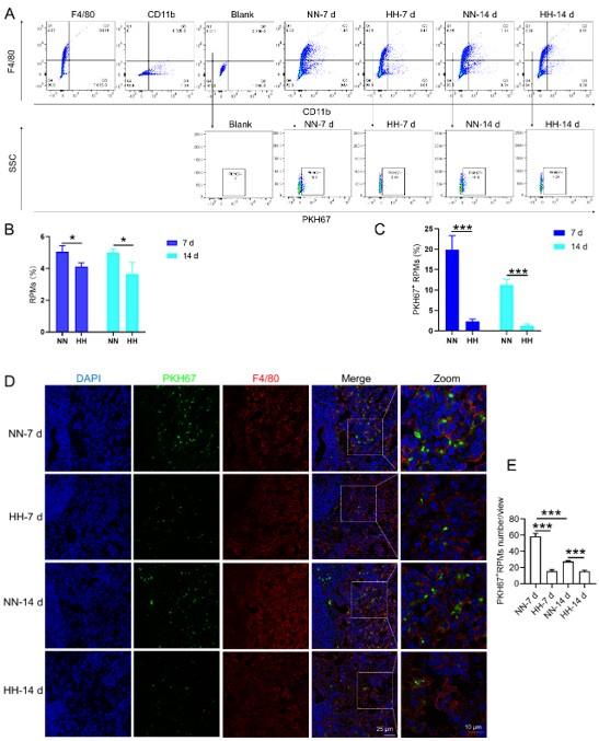
-Experiment 2 (erythrophagocytosis enhancement)
To examine the effects of enhanced erythrophagocytosis, we injected Tuftsin after administering PKH67-labelled RBCs. Our observations showed a significant decrease in PKH67 fluorescence in the spleen, particularly after Tuftsin injection compared to the NN group. This result suggests a reduction in RBC lifespan when erythrophagocytosis is enhanced (illustrated in new Figure 7, A-B).
Author response image 2.
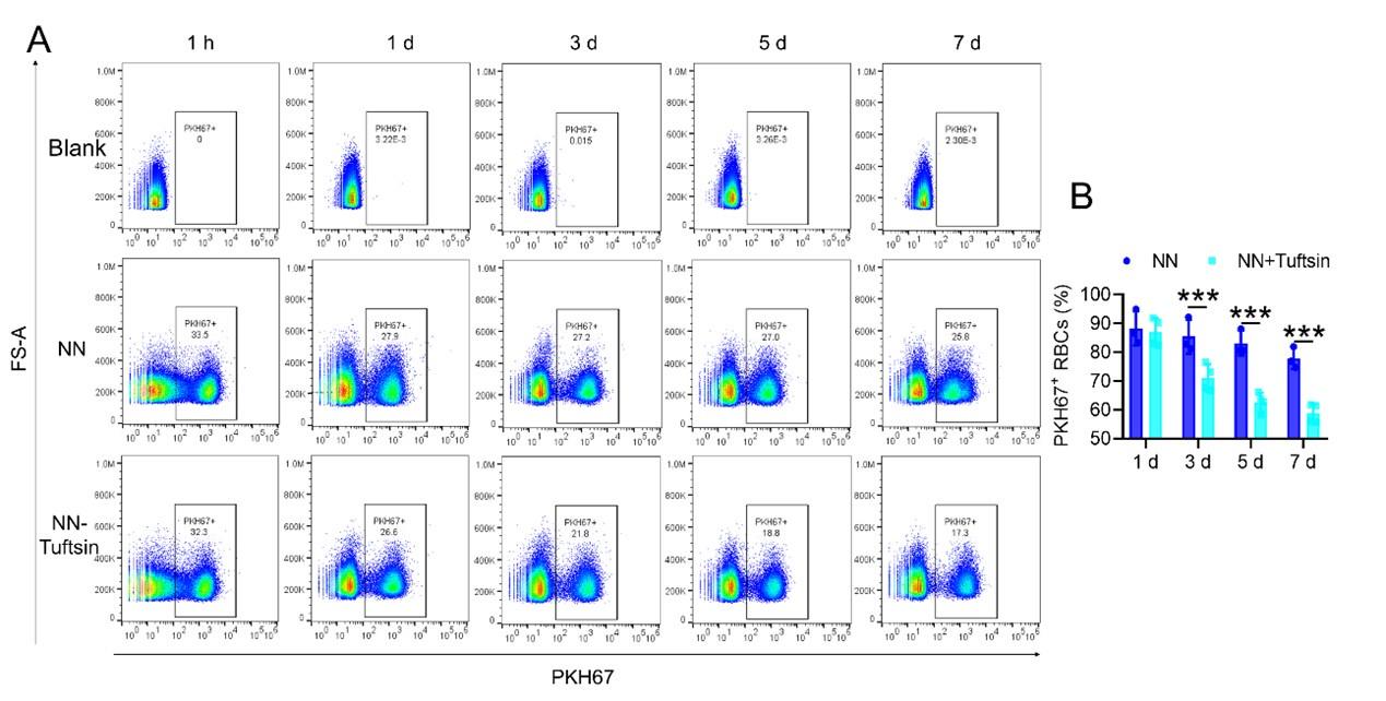
(3) Revised conclusions:
The additional data from these experiments support our original findings by providing a more comprehensive view of the impact of HH exposure on splenic erythrophagocytosis.
The decrease in phagocytic RPMs and phagocytic erythrocytes after HH exposure, along with the observed decrease in RBC lifespan following enhanced erythrophagocytosis, collectively suggest a more complex interplay between hypoxia, erythrophagocytosis, and RBC lifespan than initially interpreted.
We think that these revisions and additional experimental data provide a more robust and detailed understanding of the effects of HH on splenic erythrophagocytosis and RBCs lifespan. We hope that these changes adequately address the concerns raised and strengthen the conclusions drawn in our manuscript.
(2) F4/80 high; CD11b low are true RPMs which the cells which the authors are presenting, i.e. splenic monocytes / pre-RPMs. To discuss RPM function requires the presentation of these cells specifically rather than general cells in the proper area of the spleen.
Thank you for your feedback requesting a substantial revision of our claims and interpretation, particularly considering additional data showing enhanced erythrophagocytosis with decreased RBC lifespan. In response, we have thoroughly revised our manuscript and included new experimental data that further elucidate the effects of HH on RPMs and erythrophagocytosis.
(1) Re-evaluation of RPMs population after HH exposure:
Author response image 3.
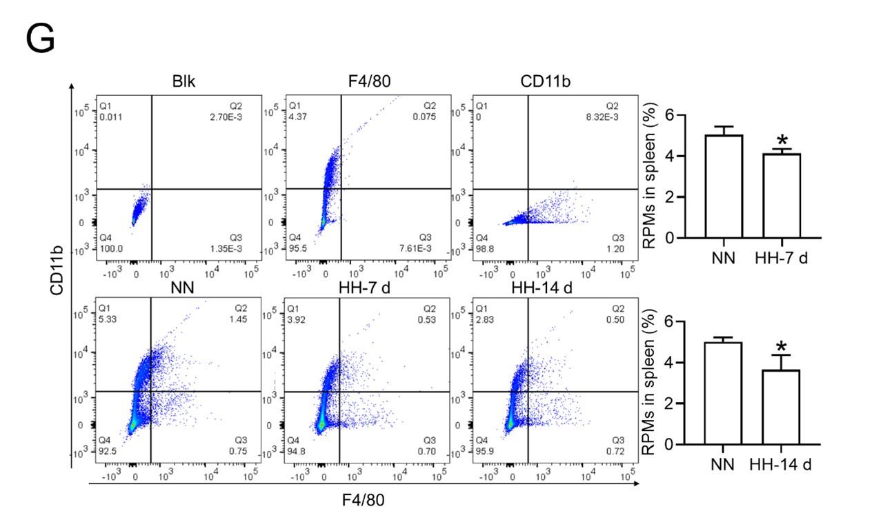
Author response image 4.
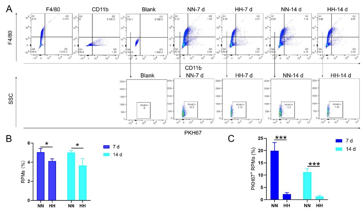
We further confirmed the decreased population of RPMs through in situ co-staining with F4/80 and CD11b, and F4/80 and CD68, in spleen tissues. These results clearly demonstrated a significant reduction in F4/80hiCD11blo (Figure S1, A and B) and F4/80hiCD68hi (Figure S1, C and D) cells following HH exposure.
Author response image 5.
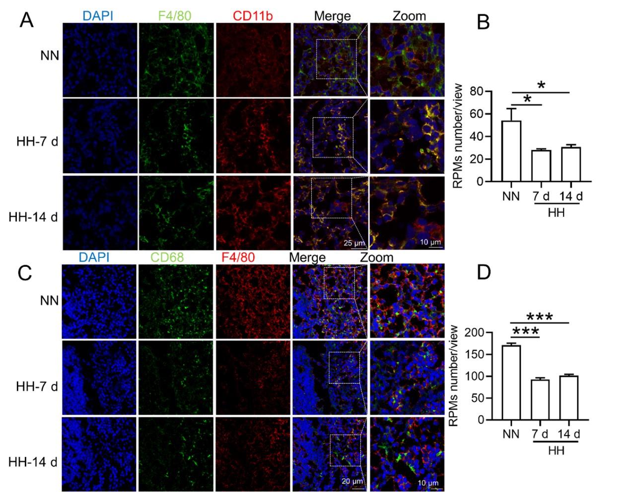
(2) Single-cell sequencing analysis of splenic RPMs:
We conducted a single-cell sequencing analysis of spleen samples post 7 days of HH exposure (Figure S2, A-C). This analysis revealed a notable shift in the distribution of RPMs, predominantly associated with Cluster 0 under NN conditions, to a reduced presence in this cluster after HH exposure.
Pseudo-time series analysis indicated a transition pattern change in spleen RPMs, with a shift from Cluster 2 and Cluster 1 towards Cluster 0 under NN conditions, and a reverse transition following HH exposure (Figure S2, B and D). This finding implies a decrease in resident RPMs in the spleen under HH conditions.
(3) Consolidated findings and revised interpretation:
The comprehensive analysis of flow cytometry, in situ staining, and single-cell sequencing data consistently indicates a significant reduction in the number of RPMs following HH exposure.
These findings, taken together, strongly support the revised conclusion that HH exposure leads to a decrease in RPMs in the spleen, which in turn may affect erythrophagocytosis and RBC lifespan.
Author response image 6.
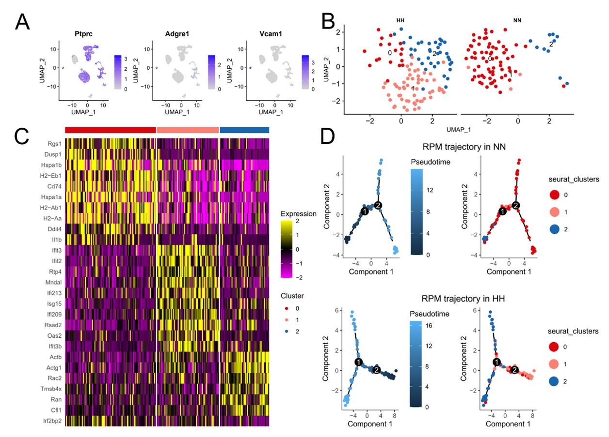
In conclusion, our revised manuscript now includes additional experimental data and analyses, strengthening our claims and providing a more nuanced interpretation of the impact of HH on spleen RPMs and related erythrophagocytosis processes. We believe these revisions and additional data address your concerns and enhance the scientific validity of our study.
(3) RBC retention in the spleen should be measured anyway quantitatively, eg, with proper flow cytometry, to determine whether it is increased or decreased.
Thank you for your query regarding the quantitative measurement of RBC retention in the spleen, particularly in relation to HH exposure. We have utilized a combination of techniques, including flow cytometry and histological staining, to investigate this aspect comprehensively. Below is a summary of our findings and methodology.
(1) Flow cytometry analysis of labeled RBCs:
Our study employed both NHS-biotin (new Figure 4, A-D) and PKH67 labeling (new Figure 4, E-H) to track RBCs in mice exposed to HH. Flow cytometry results from these experiments (new Figure 4, A-H) showed a decrease in the proportion of labeled RBCs over time, both in the blood and spleen. Notably, there was a significantly greater reduction in the amplitude of fluorescently labeled RBCs after NN exposure compared to the reduced amplitude of fluorescently labeled RBCs observed in blood and spleen under HH exposure. The observed decrease in labeled RBCs was initially counterintuitive, as we expected an increase in RBC retention due to reduced erythrophagocytosis. However, this decrease can be attributed to the significantly increased production of RBCs following HH exposure, diluting the proportion of labeled cells.
Specifically, for blood, the biotin-labeled RBCs decreased by 12.06% under NN exposure and by 7.82% under HH exposure, while the PKH67-labeled RBCs decreased by 9.70% under NN exposure and by 4.09% under HH exposure. For spleen, the biotin-labeled RBCs decreased by 3.13% under NN exposure and by 0.46% under HH exposure, while the PKH67-labeled RBCs decreased by 1.16% under NN exposure and by 0.92% under HH exposure. These findings suggest that HH exposure leads to a decrease in the clearance rate of RBCs.
Author response image 7.
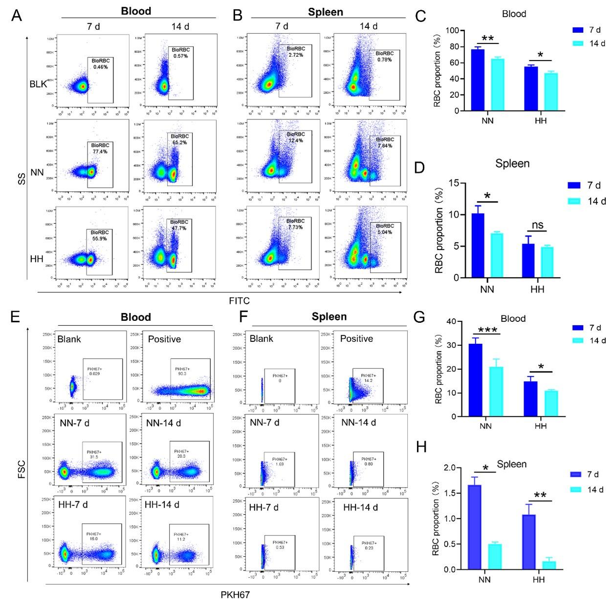
(2) Detection of erythrophagocytosis in spleen:
To assess erythrophagocytosis directly, we labeled RBCs with PKH67 and analyzed their uptake by splenic macrophages (F4/80hi) after HH exposure. Our findings (new Figure 5, D-E) indicated a decrease in PKH67-positive macrophages in the spleen, suggesting reduced erythrophagocytosis.
Author response image 8.
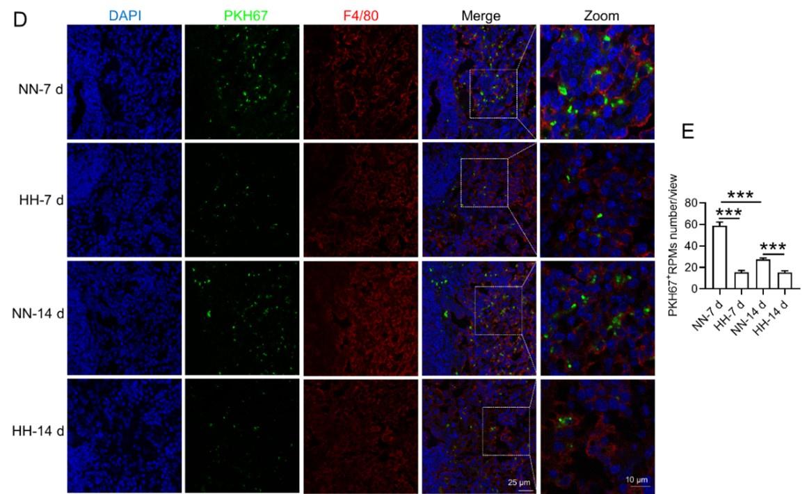
(3) Flow cytometry analysis of RBC retention:
Our flow cytometry analysis revealed a decrease in PKH67-positive RBCs in both blood and spleen (Figure S4). We postulated that this was due to increased RBC production after HH exposure. However, this method might not accurately reflect RBC retention, as it measures the proportion of PKH67-labeled RBCs relative to the total number of RBCs, which increased after HH exposure.
Author response image 9.
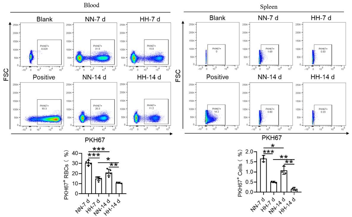
(4) Histological and immunostaining analysis:
Histological examination using HE staining and band3 immunostaining in situ (new Figure 6, A-D, and G-H) revealed a significant increase in RBC numbers in the spleen after HH exposure. This was further confirmed by detecting retained RBCs in splenic single cells using Wright-Giemsa composite stain (new Figure 6, E and F) and retained PKH67-labelled RBCs in spleen (new Figure 6, I and J).
Author response image 10.
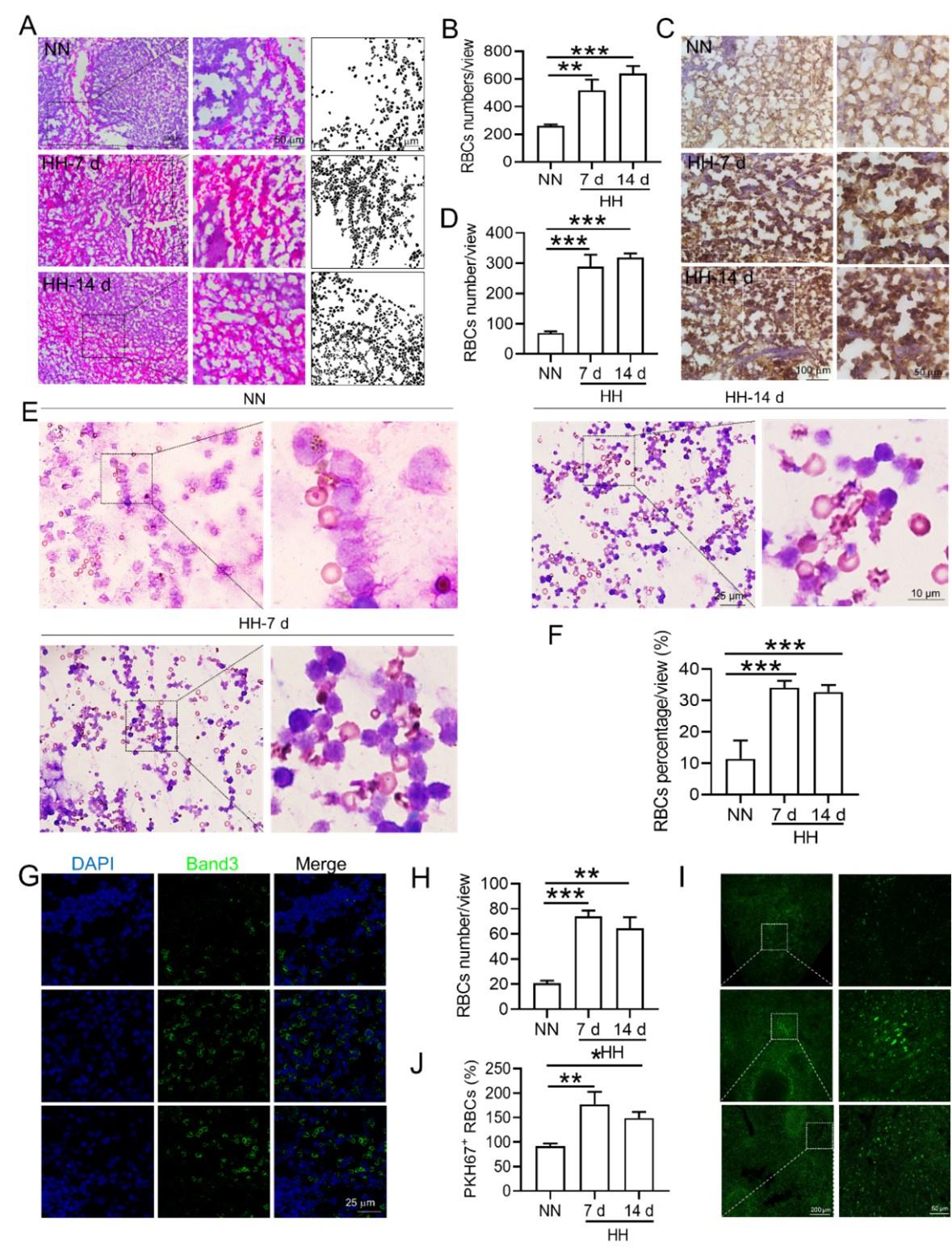
(5) Interpreting the data:
The comprehensive analysis suggests a complex interplay between increased RBC production and decreased erythrophagocytosis in the spleen following HH exposure. While flow cytometry indicated a decrease in the proportion of labeled RBCs, histological and immunostaining analyses demonstrated an actual increase in RBCs retention in the spleen. These findings collectively suggest that while the overall RBCs production is upregulated following HH exposure, the spleen's capacity for erythrophagocytosis is concurrently diminished, leading to increased RBCs retention.
(6) Conclusion:
Taken together, our results indicate a significant increase in RBCs retention in the spleen post-HH exposure, likely due to reduced residual RPMs and erythrophagocytosis. This conclusion is supported by a combination of flow cytometry, histological staining, and immunostaining techniques, providing a comprehensive view of RBC dynamics under HH conditions. We think these findings offer a clear quantitative measure of RBC retention in the spleen, addressing the concerns raised in your question.
(4) Numerous other methodological problems as listed below.
We appreciate your question, which highlights the importance of using multiple analytical approaches to understand complex physiological processes. Please find below our point-by-point response to the methodological comments.
Reviewer #1 (Recommendations For The Authors):
(1) Decreased BM and spleen monocytes d/t increased liver monocyte migration is unclear. there is no evidence that this happens or why it would be a reasonable hypothesis, even in splenectomized mice.
Thank you for highlighting the need for further clarification and justification of our hypothesized decrease in BM and spleen monocytes due to increased monocyte migration to the liver, particularly in the context of splenectomized mice. Indeed, our study has not explicitly verified an augmentation in mononuclear cell migration to the liver in splenectomized mice.
Nonetheless, our investigations have revealed a notable increase in monocyte migration to the liver after HH exposure. Noteworthy is our discovery of a significant upregulation in colony stimulating factor-1 (CSF-1) expression in the liver, observed after both 7 and 14 days of HH exposure (data not included). This observation was substantiated through flow cytometry analysis (as depicted in Figure S4), which affirmed an enhanced migration of monocytes to the liver. Specifically, we noted a considerable increase in the population of transient macrophages, monocytes, and Kupffer cells in the liver following HH exposure.
Author response image 11.
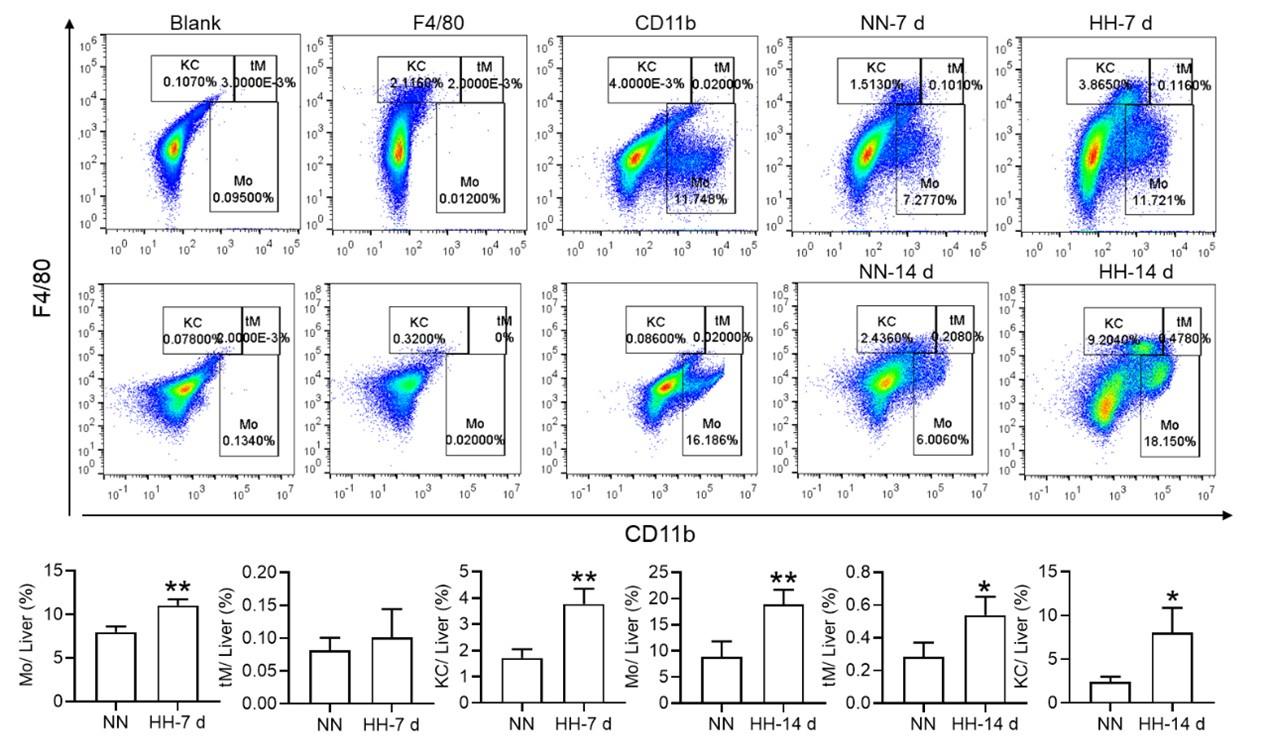
Considering these findings, we hypothesize that hypoxic conditions may activate a compensatory mechanism that directs monocytes towards the liver, potentially linked to the liver’s integral role in the systemic immune response. In accordance with these insights, we intend to revise our manuscript to reflect the speculative nature of this hypothesis more accurately, and to delineate the strategies we propose for its further empirical investigation. This amendment ensures that our hypothesis is presented with full consideration of its speculative basis, supported by a coherent framework for future validation.
(2) While F4/80+CD11b+ population is decreased, this is mainly driven by CD11b and F4/80+ alone population is significantly increased. This is counter to the hypothesis.
Thank you for addressing the apparent discrepancy in our findings concerning the F4/80+CD11b+ population and the increase in the F4/80+ alone population, which seems to contradict our initial hypothesis. Your observation is indeed crucial for the integrity of our study, and we appreciate the opportunity to clarify this matter.
(1) Clarification of flow cytometry results:
In response to the concerns raised, we revisited our flow cytometry experiments with a focus on more clearly distinguishing the cell populations. Our initial graph had some ambiguities in cell grouping, which might have led to misinterpretations.
The revised flow cytometry analysis, specifically aimed at identifying red pulp macrophages (RPMs) characterized as F4/80hiCD11blo in the spleen, demonstrated a significant decrease in the F4/80 population. This finding is now in alignment with our immunofluorescence results.
Author response image 12.

Author response image 13.
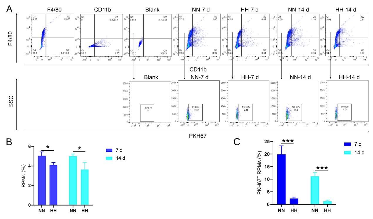
(2) Revised data and interpretation:
We’ve updated our manuscript to reflect these new findings and interpretations. The revised manuscript details the revised flow cytometry analysis and discusses the potential mechanisms behind the observed changes in macrophage populations.
(3) HO-1 expression cannot be used as a surrogate to quantify number of macrophages as the expression per cell can decrease and give the same results. In addition, the localization of effect to the red pulp is not equivalent to an assertion that the conclusion applies to macrophages given the heterogeneity of this part of the organ and the spleen in general.
Thank you for your insightful comments regarding the use of HO-1 expression as a surrogate marker for quantifying macrophage numbers, and for pointing out the complexity of attributing changes in HO-1 expression specifically to macrophages in the splenic red pulp. Your observations are indeed valid and warrant a detailed response.
(1) Role of HO-1 in macrophage activity:
In our study, HO-1 expression was not utilized as a direct marker for quantifying macrophages. Instead, it was considered an indicator of macrophage activity, particularly in relation to erythrophagocytosis. HO-1, being upregulated in response to erythrophagocytosis, serves as an indirect marker of this process within splenic macrophages.
The rationale behind this approach was that increased HO-1 expression, induced by erythrophagocytosis in the spleen’s red pulp, could suggest an augmentation in the activity of splenic macrophages involved in this process.
(2) Limitations of using HO-1 as an indicator:
We acknowledge your point that HO-1 expression per cell might decrease, potentially leading to misleading interpretations if used as a direct quantifier of macrophage numbers. The variability in HO-1 expression per cell indeed presents a limitation in using it as a sole indicator of macrophage quantity.
Furthermore, your observation about the heterogeneity of the spleen, particularly the red pulp, is crucial. The red pulp is a complex environment with various cell types, and asserting that changes in HO-1 expression are exclusive to macrophages could oversimplify this complexity.
(3) Addressing the concerns:
To address these concerns, we propose to supplement our HO-1 expression data with additional specific markers for macrophages. This would help in correlating HO-1 expression more accurately with macrophage numbers and activity.
We also plan to conduct further studies to delineate the specific cell types in the red pulp contributing to HO-1 expression. This could involve techniques such as immunofluorescence or immunohistochemistry, which would allow us to localize HO-1 expression to specific cell populations within the splenic red pulp.
We’ve revised our manuscript to clarify the role of HO-1 expression as an indirect marker of erythrophagocytosis and to acknowledge its limitations as a surrogate for quantifying macrophage numbers.
(4) line 63-65 is inaccurate as red cell homeostasis reaches a new steady state in chronic hypoxia.
Thank you for pointing out the inaccuracy in lines 63-65 of our manuscript regarding red cell homeostasis in chronic hypoxia. Your feedback is invaluable in ensuring the accuracy and scientific integrity of our work. We’ve revised lines 63-65 to accurately reflect the understanding.
(5) Eryptosis is not defined in the manuscript.
Thank you for highlighting the omission of a definition for eryptosis in our manuscript. We acknowledge the significance of precisely defining such key terminologies, particularly when they play a crucial role in the context of our research findings. Eryptosis, a term referenced in our study, is a specialized form of programmed cell death unique to erythrocytes. Similar with apoptosis in other cell types, eryptosis is characterized by distinct physiological changes including cell shrinkage, membrane blebbing, and the externalization of phosphatidylserine on the erythrocyte surface. These features are indicative of the RBCs lifecycle and its regulated destruction process.
However, it is pertinent to note that our current study does not extensively delve into the mechanisms or implications of eryptosis. Our primary focus has been to elucidate the effects of HH exposure on the processes of splenic erythrophagocytosis and the resultant impact on the lifespan of RBCs. Given this focus, and to maintain the coherence and relevance of our manuscript, we have decided to exclude specific discussions of eryptosis from our revised manuscript. This decision aligns with our aim to provide a clear and concentrated exploration of the influence of HH exposure on RBCs dynamics and splenic function.
We appreciate your input, which has significantly contributed to enhancing the clarity and accuracy of our manuscript. The revision ensures that our research is presented with a focused scope, aligning closely with our experimental investigations and findings.
(6) Physiologically, there is no evidence that there is any "free iron" in cells, making line 89 point inaccurate.
Thank you for highlighting the concern regarding the reference to "free iron" in cells in line 89 of our manuscript. The term "free iron" in our manuscript was intended to refer to divalent iron (Fe2+), rather than unbound iron ions freely circulating within cells. We acknowledge that the term "free iron" might lead to misconceptions, as it implies the presence of unchelated iron, which is not physiologically common due to the potential for oxidative damage. To rectify this and provide clarity, we’ve revised line 89 of our manuscript to reflect our meaning more accurately. Instead of "free iron," we use "divalent iron (Fe2+)" to avoid any misunderstanding regarding the state of iron in cells. We also ensure that any implications drawn from the presence of Fe2+ in cells are consistent with current scientific literature and understanding.
(7) Fig 1f no stats
We appreciate your critical review and suggestions, which help in improving the accuracy and clarity of our research. We’ve revised statistic diagram of new Figure 1F.
(8) Splenectomy experiments demonstrate that erythrophagocytosis is almost completely replaced by functional macrophages in other tissues (likely Kupffer cells in the liver). there is only a minor defect and no data on whether it is in fact the liver or other organs that provide this replacement function and makes the assertions in lines 345-349 significantly overstated.
Thank you for your critical assessment of our interpretation of the splenectomy experiments, especially concerning the role of erythrophagocytosis by macrophages in other tissues, such as Kupffer cells in the liver. We appreciate your observation that our assertions may be overstated and acknowledge the need for more specific data to identify which organs compensate for the loss of splenic erythrophagocytosis.
(1) Splenectomy experiment findings:
Our findings in Figure 2D do indicate that in the splenectomized group under NN conditions, erythrophagocytosis is substantially compensated for by functional macrophages in other tissues. This is an important observation that highlights the body's ability to adapt to the loss of splenic function.
However, under HH conditions, our data suggest that the spleen plays an important role in managing erythrocyte turnover, as indicated by the significant impact of splenectomy on erythrophagocytosis and subsequent erythrocyte dynamics.
(2) Addressing the lack of specific organ identification:
We acknowledge that our study does not definitively identify which organs, such as the liver or others, take over the erythrophagocytosis function post-splenectomy. This is an important aspect that needs further investigation.
To address this, we also plan to perform additional experiments that could more accurately point out the specific tissues compensating for the loss of splenic erythrophagocytosis. This could involve tracking labeled erythrocytes or using specific markers to identify macrophages actively engaged in erythrophagocytosis in various organs.
(3) Revising manuscript statements:
Considering your feedback, we’ve revised the statements in lines 345-349 (lines 378-383 in revised manuscript) to enhance the scientific rigor and clarity of our research presentation.
(9) M1 vs M2 macrophage experiments are irrelevant to the main thrust of the manuscript, there are no references to support the use of only CD16 and CD86 for these purposes, and no stats are provided. It is also unclear why bone marrow monocyte data is presented and how it is relevant to the rest of the manuscript.
Thank you for your critical evaluation of the relevance and presentation of the M1 vs. M2 macrophage experiments in our manuscript. We appreciate your insights, especially regarding the use of specific markers and the lack of statistical analysis, as well as the relevance of bone marrow monocyte data to our study's main focus.
(1) Removal of M1 and M2 macrophage data:
Based on your feedback and our reassessment, we agree that the results pertaining to M1 and M2 macrophages did not align well with the main objectives of our manuscript. Consequently, we have decided to remove the related content on M1 and M2 macrophages from the revised manuscript. This decision was made to ensure that our manuscript remains focused and coherent, highlighting our primary findings without the distraction of unrelated or insufficiently supported data.
The use of only CD16 and CD86 markers for M1 and M2 macrophage characterization, without appropriate statistical analysis, was indeed a methodological limitation. We recognize that a more comprehensive set of markers and rigorous statistical analysis would be necessary for a meaningful interpretation of M1/M2 macrophage polarization. Furthermore, the relevance of these experiments to the central theme of our manuscript was not adequately established. Our study primarily focuses on erythrophagocytosis and red pulp macrophage dynamics under hypobaric hypoxia, and the M1/M2 polarization aspect did not contribute significantly to this narrative.
(2) Clarification on bone marrow monocyte data:
Regarding the inclusion of bone marrow monocyte data, we acknowledge that its relevance to the main thrust of the manuscript was not clearly articulated. In the revised manuscript, we provide a clearer rationale for its inclusion and how it relates to our primary objectives.
(3) Commitment to clarity and relevance:
We are committed to ensuring that every component of our manuscript contributes meaningfully to our overall objectives and research questions. Your feedback has been instrumental in guiding us to streamline our focus and present our findings more effectively.
We appreciate your valuable feedback, which has led to a more focused and relevant presentation of our research. These changes enhance the clarity and impact of our manuscript, ensuring that it accurately reflects our key research findings.
(10) Biotinolated RBC clearance is enhanced, demonstrating that RBC erythrophagocytosis is in fact ENHANCED, not diminished, calling into question the founding hypothesis that the manuscript proposes.
Thank you for your critical evaluation of our data on biotinylated RBC clearance, which suggests enhanced erythrophagocytosis under HH conditions. This observation indeed challenges our founding hypothesis that erythrophagocytosis is diminished in this setting. Below is a summary of our findings and methodology.
(1) Interpretation of RBC labeling results:
Both the previous results of NHS-biotin labeled RBCs (new Figure 4, A-D) and the current results of PKH67-labeled RBCs (new Figure 4, E-H) demonstrated a decrease in the number of labeled RBCs with an increase in injection time. The production of RBCs, including bone marrow and spleen production, was significantly increased following HH exposure, resulting in a consistent decrease in the proportion of labeled RBCs via flow cytometry detection both in the blood and spleen of mice compared to the NN group. However, compared to the reduced amplitude of fluorescently labeled RBCs observed in blood and spleen under NN exposure, there was a significantly weaker reduction in the amplitude of fluorescently labeled RBCs after HH exposure. Specifically, for blood, the biotin-labeled RBCs decreased by 12.06% under NN exposure and by 7.82% under HH exposure, while the PKH67-labeled RBCs decreased by 9.70% under NN exposure and by 4.09% under HH exposure. For spleen, the biotin-labeled RBCs decreased by 3.13% under NN exposure and by 0.46% under HH exposure, while the PKH67-labeled RBCs decreased by 1.16% under NN exposure and by 0.92% under HH exposure.
Author response image 14.
(2) Increased RBCs production under HH conditions:
It's important to note that RBCs production, including from bone marrow and spleen, was significantly increased following HH exposure. This increase in RBCs production could contribute to the decreased proportion of labeled RBCs observed in flow cytometry analyses, as there are more unlabeled RBCs diluting the proportion of labeled cells in the blood and spleen.
(3) Analysis of erythrophagocytosis in RPMs:
Our analysis of PKH67-labeled RBCs content within RPMs following HH exposure showed a significant reduction in the number of PKH67-positive RPMs in the spleen (new Figure 5). This finding suggests a decrease in erythrophagocytosis by RPMs under HH conditions.
Author response image 15.
(4) Reconciling the findings:
The apparent contradiction between enhanced RBC clearance (suggested by the reduced proportion of labeled RBCs) and reduced erythrophagocytosis in RPMs (indicated by fewer PKH67-positive RPMs) may be explained by the increased overall production of RBCs under HH. This increased production could mask the actual erythrophagocytosis activity in terms of the proportion of labeled cells. Therefore, while the proportion of labeled RBCs decreases more significantly under HH conditions, this does not necessarily indicate an enhanced erythrophagocytosis rate, but rather an increased dilution effect due to higher RBCs turnover.
(5) Revised interpretation and manuscript changes:
Given these factors, we update our manuscript to reflect this detailed interpretation and clarify the implications of the increased RBCs production under HH conditions on our observations of labeled RBCs clearance and erythrophagocytosis. We appreciate your insightful feedback, which has prompted a careful re-examination of our data and interpretations. We hope that these revisions provide a more accurate and comprehensive understanding of the effects of HH on erythrophagocytosis and RBCs dynamics.
(11) Legend in Fig 4c-4d looks incorrect and Fig 4e-4f is very non-specific since Wright stain does not provide evidence of what type of cells these are and making for a significant overstatement in the contribution of this data to "confirming" increased erythrophagocytosis in the spleen under HH exposure (line 395-396).
Thank you for your insightful observations regarding the data presentation and figure legends in our manuscript, particularly in relation to Figure 4 (renamed as Figure 6 in the revised manuscript) and the use of Wright-Giemsa composite staining. We appreciate your constructive feedback and acknowledge the importance of presenting our data with utmost clarity and precision.
(1) Amendments to Figure legends:
We recognize the necessity of rectifying inaccuracies in the legends of the previously labeled Figure 4C and D. Corrections have been meticulously implemented to ensure the legends accurately contain the data presented. Additionally, we acknowledge the error concerning the description of Wright staining. The method employed in our study is Wright-Giemsa composite staining, which, unlike Wright staining that solely stains cytoplasm (RBC), is capable of staining both nuclei and cytoplasm.
(2) Addressing the specificity of Wright-Giemsa Composite staining:
Our approach involved quantifying RBC retention using Wright-Giemsa composite staining on single splenic cells post-perfusion at 7 and 14 days post HH exposure. We understand and appreciate your concerns regarding the nonspecific nature of Wright staining. Although Wright stain is a general hematologic stain and not explicitly specific for certain cell types, its application in our study aimed to provide preliminary insights. The spleen cells, devoid of nuclei and thus likely to be RBCs, were stained and observed post-perfusion, indicating RBC retention within the spleen.
(3) Incorporating additional methods for RBC identification:
To enhance the specificity of our findings, we integrated supplementary methods for RBC identification in the revised manuscript. We employed band3 immunostaining (in the new Figure 6, C-D and G-H) and PKH67 labeling (Figure 6, I-J) for a more targeted identification of RBCs. Band3, serving as a reliable marker for RBCs, augments the specificity of our immunostaining approach. Likewise, PKH67 labeling affords a direct and definitive means to assess RBC retention in the spleen following HH exposure.
Author response image 16. same as 10
(4) Revised interpretation and manuscript modifications:
Based on these enhanced methodologies, we have refined our interpretation of the data and accordingly updated the manuscript. The revised narrative underscores that our conclusions regarding reduced erythrophagocytosis and RBC retention under HH conditions are corroborated by not only Wright-Giemsa composite staining but also by band3 immunostaining and PKH67 labeling, each contributing distinctively to our comprehensive understanding.
We are committed to ensuring that our manuscript precisely reflects the contribution of each method to our findings and conclusions. Your thorough review has been invaluable in identifying and rectifying areas for improvement in our research report and interpretation.
(12) Ferroptosis data in Fig 5 is not specific to macrophages and Fer-1 data confirms the expected effect of Fer-1 but there is no data that supports that Fer-1 reverses the destruction of these cells or restores their function in hypoxia. Finally, these experiments were performed in peritoneal macrophages which are functionally distinct from splenic RPM.
Thank you for your critique of our presentation and interpretation of the ferroptosis data in Figure 5 (renamed as Figure 9 in the revised manuscript), as well as your observations regarding the specificity of the experiments to macrophages and the effects of Fer-1. We value your input and acknowledge the need to clarify these aspects in our manuscript.
(1) Clarification on cell type used in experiments:
(2) Specificity of ferroptosis data:
We recognize that the data presented in Figure 9 need to be more explicitly linked to the specific macrophage population being studied. In the revised manuscript, we ensure that the discussion around ferroptosis data is clearly situated within the framework of splenic macrophages.
We also provide additional methodological details in the 'Methods' section to reinforce the specificity of our experiments to splenic macrophages.
(3) Effects of Fer-1 on macrophage function and survival:
Regarding the effect of Fer-1, we agree that while our data confirms the expected effect of Fer-1 in inhibiting ferroptosis, we have not provided direct evidence that Fer-1 reverses the destruction of macrophages or restores their function in hypoxia.
To address this, we propose additional experiments to specifically investigate the impact of Fer-1 on the survival and functional restoration of splenic macrophages under hypoxic conditions. This would involve assessing not only the inhibition of ferroptosis but also the recovery of macrophage functionality post-treatment.
(4) Revised interpretation and manuscript changes:
We’ve revised the relevant sections of our manuscript to reflect these clarifications and proposed additional studies. This includes modifying the discussion of the ferroptosis data to more accurately represent the cell types involved and the limitations of our current findings regarding the effects of Fer-1.
The revised manuscript presents a more detailed interpretation of the ferroptosis data, clearly describing what our current experiments demonstrate and what remains to be investigated.
We are grateful for your insightful feedback, which has highlighted important areas for improvement in our research presentation. We think that these revisions will enhance the clarity and scientific accuracy of our manuscript, ensuring that our findings and conclusions are well-supported and precisely communicated.
Reviewer #2 (Recommendations For The Authors):
The following questions and remarks should be considered by the authors:
(1) The methods should clearly state whether the HH was discontinued during the 7 or 14 day exposure for cleaning, fresh water etc. Moreover, how was CO2 controlled? The procedure for splenectomy needs to be described in the methods.
Thank you for your inquiry regarding the specifics of our experimental methods, particularly the management of HH exposure and the procedure for splenectomy. We appreciate your attention to detail and the importance of these aspects for the reproducibility and clarity of our research.
(1) HH exposure conditions:
In our experiments, mice were continuously exposed to HH for the entire duration of 7 or 14 days, without interruption for activities such as cleaning or providing fresh water. This uninterrupted exposure was crucial for maintaining consistent hypobaric conditions throughout the experiment. The hypobaric chamber was configured to ensure a ventilation rate of 25 air exchanges per minute. This high ventilation rate was effective in regulating the concentration of CO2 inside the chamber, thereby maintaining a stable environment for the mice.
(2) The splenectomy was performed as follows:
After anesthesia, the mice were placed in a supine position, and their limbs were fixed. The abdominal operation area was skinned, disinfected, and covered with a sterile towel. A median incision was made in the upper abdomen, followed by laparotomy to locate the spleen. The spleen was then carefully pulled out through the incision. The arterial and venous directions in the splenic pedicle were examined, and two vascular forceps were used to clamp all the tissue in the main cadre of blood vessels below the splenic portal. The splenic pedicle was cut between the forceps to remove the spleen. The end of the proximal hepatic artery was clamped with a vascular clamp, and double or through ligation was performed to secure the site. The abdominal cavity was then cleaned to ensure there was no bleeding at the ligation site, and the incision was closed. Post-operatively, the animals were housed individually. Generally, they were able to feed themselves after recovering from anesthesia and did not require special care.
We hope this detailed description addresses your queries and provides a clear understanding of the experimental conditions and procedures used in our study. These methodological details are crucial for ensuring the accuracy and reproducibility of our research findings.
(2) The lack of changes in MCH needs explanation? During stress erythropoiesis some limit in iron availability should cause MCH decrease particularly if the authors claim that macrophages for rapid iron recycling are decreased. Fig 1A is dispensable. Fig 1G NN control 14 days does not make sense since it is higher than 7 days of HH.
Thank you for your inquiry regarding the lack of changes in Mean Corpuscular Hemoglobin (MCH) in our study, particularly in the context of stress erythropoiesis and decreased macrophage-mediated iron recycling. We appreciate the opportunity to provide further clarification on this aspect.
(1) Explanation for stable MCH levels:
Our research identified a decrease in erythrophagocytosis and iron recycling in the spleen following HH exposure. Despite this, the MCH levels remained stable. This observation can be explained by considering the compensatory roles of other organs, particularly the liver and duodenum, in maintaining iron homeostasis.
Specifically, our investigations revealed an enhanced capacity of the liver to engulf RBCs and process iron under HH conditions. This increased hepatic erythrophagocytosis likely compensates for the reduced splenic activity, thereby stabilizing MCH levels.
(2) Role of hepcidin and DMT1 expression:
Additionally, hypoxia is known to influence iron metabolism through the downregulation of Hepcidin and upregulation of Divalent Metal Transporter 1 (DMT1) expression. These alterations lead to enhanced intestinal iron absorption and increased blood iron levels, further contributing to the maintenance of MCH levels despite reduced splenic iron recycling.
(3) Revised Figure 1 and data presentation
To address the confusion regarding the data presented in Figure 1G, we have made revisions in our manuscript. The original Figure 1G, which did not align with the expected trends, has been removed. In its place, we have included a statistical chart of Figure 1F in the new version of Figure 1G. This revision will provide a clearer and more accurate representation of our findings.
(4) Manuscript updates and future research:
We update our manuscript to incorporate these explanations, ensuring that the rationale behind the stable MCH levels is clearly articulated. This includes a discussion on the role of the liver and duodenum in iron metabolism under hypoxic conditions.
Future research could explore in greater detail the mechanisms by which different organs contribute to iron homeostasis under stress conditions like HH, particularly focusing on the dynamic interplay between hepatic and splenic functions.
We thank you for your insightful question, which has prompted a thorough re-examination of our findings and interpretations. We believe that these clarifications will enhance the overall understanding of our study and its implications in the context of iron metabolism and erythropoiesis under hypoxic conditions.
(3) Fig 2 the difference between sham and splenectomy is really marginal and not convincing. Is there also a difference at 7 days? Why does the spleen size decrease between 7 and 14 days?
Thank you for your observations regarding the marginal differences observed between sham and splenectomy groups in Figure 2, as well as your inquiries about spleen size dynamics over time. We appreciate this opportunity to clarify these aspects of our study.
(1) Splenectomy vs. Sham group differences:
(2) Spleen size dynamics and peak stress erythropoiesis:
The observed splenic enlargement prior to 7 days can be attributed to a combination of factors, including the retention of RBCs and extramedullary hematopoiesis, which is known to be a response to hypoxic stress.
Prior research has elucidated that splenic stress-induced erythropoiesis, triggered by hypoxic conditions, typically attains its zenith within a timeframe of 3 to 7 days. This observation aligns with our Toluidine Blue (TO) staining results, which indicated that the apex of this response occurs at the 7-day mark (as depicted in Figure 1, F-G). Here, the culmination of this peak is characteristically succeeded by a diminution in extramedullary hematopoiesis, a phenomenon that could elucidate the observed contraction in spleen size, particularly in the interval between 7 and 14 days.
This pattern of splenic response under prolonged hypoxic stress is corroborated by studies such as those conducted by Wang et al. (2021), Harada et al. (2015), and Cenariu et al. (2021). These references collectively underscore that the spleen undergoes significant dynamism in reaction to sustained hypoxia. This dynamism is initially manifested as an enlargement of the spleen, attributable to escalated erythropoiesis and erythrophagocytosis. Subsequently, as these processes approach normalization, a regression in spleen size ensues.
We’ve revised our manuscript to include a more detailed explanation of these splenic dynamics under HH conditions, referencing the relevant literature to provide a comprehensive context for our findings. We will also consider performing additional analysis or providing further data on spleen size changes at 7 days to support our observations and ensure a thorough understanding of the splenic response to hypoxic stress over time.
(4) Fig 3 B the clusters should be explained in detail. If the decrease in macrophages in Fig 3K/L is responsible for the effect, why does splenectomy not have a much stronger effect? How do the authors know which cells died in the calcein stained population in Fig 3D?
Thank you for your insightful questions regarding the details of our data presentation in Figure 3, particularly about the identification of cell clusters and the implications of macrophage reduction. We appreciate the opportunity to address these aspects and clarify our findings.
(1) Explanation of cell clusters in Figure 3B:
In the revised manuscript, we have included detailed notes for each cell population represented in Figure 3B (Figure 3D in revised manuscript). These notes provide a clearer understanding of the cell types present in each cluster, enhancing the interpretability of our single-cell sequencing data.
This detailed annotation will help readers to better understand the composition of the splenic cell populations under study and how they are affected by hypoxic conditions.
(2) Impact of splenectomy vs. macrophage reduction:
The interplay between the reduction in macrophage populations, as evidenced by our single-cell sequencing data, and the ramifications of splenectomy presents a multifaceted scenario. Notably, the observed decline in macrophage numbers following HH exposure does not straightforwardly equate to a comparable alteration in overall splenic function, as might be anticipated with splenectomy.
In the context of splenectomy under HH conditions, a significant escalation in the RBCs count was observed, surpassing that in non-splenectomized mice exposed to HH. This finding underscores the spleen's critical role in modulating RBCs dynamics under HH. It also indirectly suggests that the diminished phagocytic capacity of the spleen following HH exposure contributes to an augmented RBCs count, albeit to a lesser extent than in the splenectomy group. This difference is attributed to the fact that, while the number of RPMs in the spleen post-HH is reduced, they are still present, unlike in the case of splenectomy, where they are entirely absent.
Splenectomy entails the complete removal of the spleen, thus eliminating a broad spectrum of functions beyond erythrophagocytosis and iron recycling mediated by macrophages. The nuanced changes observed in our study may be reflective of the spleen's diverse functionalities and the organism's adaptive compensatory mechanisms in response to the loss of this organ.
(3) Calcein stained population in Figure 3D:
Regarding the identification of cell death in the calcein-stained population in Figure 3D (Figure 3A in revised manuscript), we acknowledge that the specific cell types undergoing death could not be distinctly determined from this analysis alone.
The calcein staining method allows for the visualization of live (calcein-positive) and dead (calcein-negative) cells, but it does not provide specific information about the cell types. The decrease in macrophage population was inferred from the single-cell sequencing data, which offered a more precise identification of cell types.
(4) Revised manuscript and data presentation:
Considering your feedback, we have revised our manuscript to provide a more comprehensive explanation of the data presented in Figure 3, including the nature of the cell clusters and the interpretation of the calcein staining results.
We have also updated the manuscript to reflect the removal of Figure 3K/L results and to provide a more focused discussion on the relevant findings.
We are grateful for your detailed review, which has helped us to refine our data presentation and interpretation. These clarifications and revisions will enhance the clarity and scientific rigor of our manuscript, ensuring that our conclusions are well-supported and accurately conveyed.
(5) Is the reduced phagocytic capacity in Fig 4B significant? Erythrophagocytosis is compromised due to the considerable spontaneous loss of labelled erythrocytes; could other assays help? (potentially by a modified Chromium release assay?). Is it necessary to stimulated phagocytosis to see a significant effect?
Thank you for your inquiry regarding the significance of the reduced phagocytic capacity observed in Figure 4B, and the potential for employing alternative assays to elucidate erythrophagocytosis dynamics under HH conditions.
(1) Significance of reduced phagocytic capacity:
The observed reduction in the amplitude of fluorescently labeled RBCs in both the blood and spleen under HH conditions suggests a decrease in erythrophagocytosis. This is indicative of a diminished phagocytic capacity, particularly when contrasted with NN conditions.
(2) Investigation of erythrophagocytosis dynamics:
To delve deeper into erythrophagocytosis under HH, we employed Tuftsin to enhance this process. Following the injection of PKH67-labeled RBCs and subsequent HH exposure, we noted a significant decrease in PKH67 fluorescence in the spleen, particularly marked after the administration of Tuftsin. This finding implies that stimulated erythrophagocytosis can influence RBCs lifespan.
(3) Erythrophagocytosis under normal and hypoxic conditions:
Under normal conditions, the reduction in phagocytic activity is less apparent without stimulation. However, under HH conditions, our findings demonstrate a clear weakening of the phagocytic effect. While we established that promoting phagocytosis under NN conditions affects RBC lifespan, the impact of enhanced phagocytosis under HH on RBCs numbers was not explicitly investigated.
(4) Potential for alternative assays:
Considering the considerable spontaneous loss of labeled erythrocytes, alternative assays such as a modified Chromium release assay could provide further insights. Such assays might offer a more nuanced understanding of erythrophagocytosis efficiency and the stability of labeled RBCs under different conditions.
(5) Future research directions:
The implications of these results suggest that future studies should focus on comparing the effects of stimulated phagocytosis under both NN and HH conditions. This would offer a clearer picture of the impact of hypoxia on the phagocytic capacity of macrophages and the subsequent effects on RBC turnover.
In summary, our findings indicate a diminished erythrophagocytic capacity, with enhanced phagocytosis affecting RBCs lifespan. Further investigation, potentially using alternative assays, would be beneficial to comprehensively understand the dynamics of erythrophagocytosis in different physiological states.
(6) Can the observed ferroptosis be influenced by bi- and not trivalent iron chelators?
Thank you for your question regarding the potential influence of bi- and trivalent iron chelators on ferroptosis under hypoxic conditions. We appreciate the opportunity to discuss the implications of our findings in this context.
(1) Analysis of iron chelators on ferroptosis:
In our study, we did not specifically analyze the effects of bi- and trivalent iron chelators on ferroptosis under hypoxia. However, our observations with Deferoxamine (DFO), a well-known iron chelator, provide some insights into how iron chelation may influence ferroptosis in splenic macrophages under hypoxic conditions.
(2) Effect of DFO on oxidative stress markers:
Our findings showed that under 1% O2, there was an increase in Malondialdehyde (MDA) content, a marker of lipid peroxidation, and a decrease in Glutathione (GSH) content, indicative of oxidative stress. These changes are consistent with the induction of ferroptosis, which is characterized by increased lipid peroxidation and depletion of antioxidants. Treatment with Ferrostatin-1 (Fer-1) and DFO effectively reversed these alterations. This suggests that DFO, like Fer-1, can mitigate ferroptosis in splenic macrophages under hypoxia, primarily by impacting MDA and GSH levels.
Author response image 17.
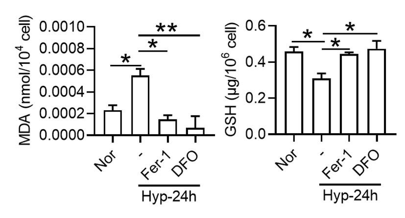
(3) Potential role of iron chelators in ferroptosis:
The effectiveness of DFO in reducing markers of ferroptosis indicates that iron availability plays a crucial role in the ferroptotic process under hypoxic conditions. It is plausible that both bi- and trivalent iron chelators could influence ferroptosis, given their ability to modulate iron availability within cells. Since ferroptosis is an iron-dependent form of cell death, chelating iron, irrespective of its valence state, could potentially disrupt the process by limiting the iron necessary for the generation of reactive oxygen species and lipid peroxidation.
(4) Additional research and manuscript updates:
Our study highlights the need for further research to explore the differential effects of various iron chelators on ferroptosis, particularly under hypoxic conditions. Such studies could provide a more comprehensive understanding of the role of iron in ferroptosis and the potential therapeutic applications of iron chelators. We update our manuscript to include these findings and discuss the potential implications of iron chelation in the context of ferroptosis under hypoxic conditions. This will provide a broader perspective on our research and its significance in understanding the mechanisms of ferroptosis.
Author response:
The following is the authors’ response to the previous reviews.
Reviewer #1 (Recommendations for The Authors):
Q1: In response to reviewers you noted totally 292 sequenced LECs, however in reviewer figure 3 B the numbers seem to add up to 221. Please include mention of the total number of LEC sequences. Please mention line 119, page 4 the total number of explored LEC transcriptomes
Thank you for your carefully review. We have updated Fig 2A, 2C and 2E. It was 242 (not 292) LECs included in our initial analysis, which contains the sample of d5 post MI in raw data (E-MTAB-7895). We dropped d5 in our subsequent analysis because the change in d5 did not significant differ from d3. Therefore, we included 221 LECs in our final analysis as we updated in Fig2A, 2C and 2E.
Q2-1: Figure 3A supposedly shows % of LEC subpopulations relative to their numbers found in day 0 samples. However, there seem to be some errors, because for example the subpop LEC Cap I include 13 cells day 1 and 6 cells day 1, which corresponds to 46% of initial numbers. However, from your graph 3B the blue population seems to occupy 10%. Please revise or explain how these relative % were calculated.
Thank you for your question. In the Figure 3A, each column was calculated by dn/d0*100%, that is d0=57/57*100%=100%, and d1= 21/57*100%=36.84%, d3=9/57*100%=15.79%, d7, d14, d28...Therefor, Cap I in d0 (13 cells) is 13/57*100%=22.81%, and Cap I in d1(6 cells) is 6/57*100%= 10.53%.
Q2-2: Further, based on the relative % of LEC subpopulations, using the numbers mentioned in Fig 3B, it would appear that the relative frequency LEC cap II population is actually stable at around 20-30% of all LECs per time point throughout the study (except day 1 drop). This contrasts with line 136 p. 4 statement. I would also urge caution for interpreting too much into the variation of relative levels of LEC co, as these represent exceeding rare cells in your samples, and could reflect technical issues rather than true biological variation (total LEC co numbers analyzed ranging from 1-24 cells/ time point). The same could be said of LEC cap II and cap III.
We strongly agree with your comment on the proportion of LEC cell subtypes post MI. As you pointed out, we have revised the result description on Page 4, line 137-143 as followed.
“In the early stages of myocardial infarction (D1 and D3), the quantity of LECs decreased sharply. The number of LECs gradually increasing from day 7 and returning to normal levels by day 14 after MI. Moreover, from day 14 onwards, the number and proportion of Ca I type LECs significantly increased.”
Q3: Please list in supplement the gene features used to identify in spatial transcriptomics the different LEC subpopulations, as their profiles (notably for capillary LECs) don't appear to be very different based on data in Fig 2F.
We have supplied gene features in supplementary materials.
Q4: In section 2.7 you refer to Gal9 secretion. Please replace with expression as no measure of protein levels from LECs has been described in your study.
Thank you for your suggestion, we have replaced secretion with expression.
Q5: The updated method to exclude non-lymphatic cells from lymphatic vessel analyses by incorporating pdpn as an additional marker ('present costained areas wherever possible' line 350 p 10)
Thank you for your correction. We have updated the description as follows and lighted them in the manuscript: rabbit anti-Lyve1 (1:300, ab14917, Abcam, UK), [Syrian hamster anti-Podoplanin (1:100, 53-5381-82, Thermo, USA), rabbit anti-Prox1(1:300, ab199359, Abcam, UK), both anti-podoplain and anti-prox1 are additional markers co-stained with Lyve1 to exclude non-lymphatic cells from lymphatic vessel].
Q6: Fig 1B, it is highly surprising to see the lymphatic density in the BZ go from 25 um² at day 3 to more than 1000 um² only four days later (day 7). Is it possible that your day 3 measurements were in the infarct area, and not BZ area? The H&E image shown in Fig1a for d3 sample would seem to indicate the analysis was done in a dead area, rather than BZ. Please revise (perhaps select similar zone as shown for d1 in fig 6D, adjusted for subepicardial region and not mid-myocardial as seems to be the case currently), and also provide lymphatic area measures in healthy myocardium for day 0 samples. The unit used (um²) also would depend on the size of the area examined. Is this unit per image? If so please report total imaged area as a reference.
A6: Thank you for your reminding and advises. We have labeled each zone on H&E and IF images in Fig1-supplementary Fig2B, and updated a clearer histological photo taken at 3 days post MI in Fig1A. Furthermore, we recalculated the lymphatic vessel area ratio as you suggested by calculating the ratio of LEC co-stained area to total imaged area under 100-fold magnification.
Q7: The mention that CD68 antibody isn't compatible with lyve1 antibody could easily have been bridged by using other macrophage markers, such as F4/80, which is readily available and often used marker for macs in mice and comes notably as a rat anti-mouse F4-80. It would have added much more relevant information to exclude Lyve1-/F4/80+ cells as compared to the current analysis, which may indeed include in area measures Lyve1+ /Pdpn- single cells erroneously spotted as 'lymphatic vessels'
Thank you for your excellent suggestion. We co-stained the sample with F4/80 and LYVE1 and supplied in the Fig1-supplementary Figure 1E, as shown in Author response image 1.
Author response image 1.
Immunofluorescence (IF) co-staining of tissue section with F4/80 and LYVE1 in sham and MI mice model at d3, d7, d14, and d28 post-MI. LYVE1: lymphatic vessel endothelial hyaluronan receptor 1; DAPI: 4’6-diamidino-2-phenylindole; scale bar in 10×-100 μm, 40×-25μm.
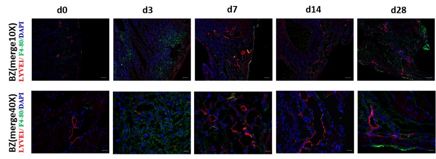
Reviewer 2 (Recommendations for The Authors):
Q1: Language expression must be improved. Many incomplete sentences exist throughout the manuscript. A few examples: Line 70-71: In order to further elucidate the effects and regulatory mechanisms of the lymphatic vessels in the repair process of myocardial injury following MI. Line 71-73. This study, integrated single-cell sequencing and spatial transcriptome data from mouse heart tissue at different timepoints after MI from publicly available data (E-MTAB-7895, GSE214611) in the ArrayExpress and gene expression omnibus (GEO) databases. Line 88-89: Since the membrane protein LYVE1 can present lymphatic vessel morphology more clearly than PROX1.
Thank you for your correction. We have carefully inspected and corrected the whole manuscript.
Q2: The type of animal models (i.e., permanent MI or MI plus reperfusion) included in Array Express and gene expression omnibus (GEO) databases must be clearly defined as these two models may have completely different effects on lymphatic vessel development during post-MI remodeling.
Thank you for your excellent suggestion. The animal models used in both E-MTAB-7895 and GSE214611 are permanent MI. We have modified the model information in the methodology section (page 12, line 400-401).
Q3: Line 119-120: Caution must be taken regarding Cav1 as a lymphocyte marker because Cav1 is expressed in all endothelial cells, not limited to LEC.
Thanks for your reminding. Cav 1 used in our clustering is one of the marker gene for its different expression in sub-types of LECs, referred in article PMID: 31402260
Q4: Figure 1 legend needs to be improved. RZ, BZ, and IZ need to be labeled in all IF images. Day 0 images suggest that RZ is the tissue section from the right ventricle.
Thank you for your suggestion. We have labeled and updated the regions of RZ, BZ, and IZ in H&E and IF image in Figure1-Figure supplement 2B.
Q5: The discussion section needs to be improved and better focused on the findings from the current study.
Thank you for your good comment. Based on your suggestion, we have revised the first paragraph of the discussion from lines 250-256 (Page 7) as followed:
Cardiac lymphatics play an important role in myocardial edema and inflammation. This study, for the first time, integrated single-cell sequencing data and spatial transcriptome data from mouse heart tissue at different time points of post-MI, and identified four transcriptionally distinct subtypes of LECs and their dynamic transcriptional heterogeneity distribution in different regions of myocardial tissue post-MI. These subgroups of LECs were shown to form different function involved in the inflammation, apoptosis, ferroptosis, and water absorption related regulation of vasopressin during the process of myocardial repair after MI.
Author response:
The following is the authors’ response to the previous reviews.
Public Reviews:
Reviewer #1 (Public review):
Summary:
In their manuscript entitled 'The domesticated transposon protein L1TD1 associates with its ancestor L1 ORF1p to promote LINE-1 retrotransposition', Kavaklıoğlu and colleagues delve into the role of L1TD1, an RNA binding protein (RBP) derived from a LINE1 transposon. L1TD1 proves crucial for maintaining pluripotency in embryonic stem cells and is linked to cancer progression in germ cell tumors, yet its precise molecular function remains elusive. Here, the authors uncover an intriguing interaction between L1TD1 and its ancestral LINE-1 retrotransposon.
The authors delete the DNA methyltransferase DNMT1 in a haploid human cell line (HAP1), inducing widespread DNA hypo-methylation. This hypomethylation prompts abnormal expression of L1TD1. To scrutinize L1TD1's function in a DNMT1 knock-out setting, the authors create DNMT1/L1TD1 double knock-out cell lines (DKO). Curiously, while the loss of global DNA methylation doesn't impede proliferation, additional depletion of L1TD1 leads to DNA damage and apoptosis.
To unravel the molecular mechanism underpinning L1TD1's protective role in the absence of DNA methylation, the authors dissect L1TD1 complexes in terms of protein and RNA composition. They unveil an association with the LINE-1 transposon protein L1-ORF1 and LINE-1 transcripts, among others.
Surprisingly, the authors note fewer LINE-1 retro-transposition events in DKO cells compared to DNMT1 KO alone.
Strengths:
The authors present compelling data suggesting the interplay of a transposon-derived human RNA binding protein with its ancestral transposable element. Their findings spur interesting questions for cancer types, where LINE1 and L1TD1 are aberrantly expressed.
Weaknesses:
Suggestions for refinement:
The initial experiment, inducing global hypo-methylation by eliminating DNMT1 in HAP1 cells, is intriguing and warrants more detailed description. How many genes experience misregulation or aberrant expression? What phenotypic changes occur in these cells? Why did the authors focus on L1TD1? Providing some of this data would be helpful to understand the rationale behind the thorough analysis of L1TD1.
The finding that L1TD1/DNMT1 DKO cells exhibit increased apoptosis and DNA damage but decreased L1 retro-transposition is unexpected. Considering the DNA damage associated with retro-transposition and the DNA damage and apoptosis observed in L1TD1/DNMT1 DKO cells, one would anticipate the opposite outcome. Could it be that the observation of fewer transposition-positive colonies stems from the demise of the most transpositionpositive colonies? Further exploration of this phenomenon would be intriguing.
Reviewer #2 (Public review):
In this study, Kavaklıoğlu et al. investigated and presented evidence for a role for domesticated transposon protein L1TD1 in enabling its ancestral relative, L1 ORF1p, to retrotranspose in HAP1 human tumor cells. The authors provided insight into the molecular function of L1TD1 and shed some clarifying light on previous studies that showed somewhat contradictory outcomes surrounding L1TD1 expression. Here, L1TD1 expression was correlated with L1 activation in a hypomethylation dependent manner, due to DNMT1 deletion in HAP1 cell line. The authors then identified L1TD1 associated RNAs using RIPSeq, which display a disconnect between transcript and protein abundance (via Tandem Mass Tag multiplex mass spectrometry analysis). The one exception was for L1TD1 itself, is consistent with a model in which the RNA transcripts associated with L1TD1 are not directly regulated at the translation level. Instead, the authors found L1TD1 protein associated with L1-RNPs and this interaction is associated with increased L1 retrotransposition, at least in the contexts of HAP1 cells. Overall, these results support a model in which L1TD1 is restrained by DNA methylation, but in the absence of this repressive mark, L1TD1 is expression, and collaborates with L1 ORF1p (either directly or through interaction with L1 RNA, which remains unclear based on current results), leads to enhances L1 retrotransposition. These results establish feasibility of this relationship existing in vivo in either development or disease, or both.
Comments on revised version:
In general, the authors did an acceptable job addressing the major concerns throughout the manuscript. This revision is much clearer and has improved in terms of logical progression.
Recommendations for the authors:
Reviewer #1 (Recommendations for the authors):
The authors have addressed all my questions in the revised version of the manuscript.
Reviewer #2 (Recommendations for the authors):
Revised comments:
A few points we'd like to see addressed are our comments about the model (Figure S7C), as this is important for the readership to understand this complex finding. Please try to apply some quantification, if possible (question 8). Please do your best to tone down the direct relationship of these findings to embryology (question 11). Based on both reviewer comments, we believe addressing reviewer #1s "Suggestions for refinement" (2 points), would help us change our view of solid to convincing.
Responses to changes:
Major
(1) The study only used one knockout (KO) cell line generated by CRISPR/Cas9.
Considering the possibility of an off-target effect, I suggest the authors attempt one or both of these suggestions.
A) Generate or acquire a similar DMNT1 deletion that uses distinct sgRNAs, so that the likelihood of off-targets is negligible. A few simple experiments such as qRT-PCR would be sufficient to suggest the same phenotype.
B) Confirm the DNMT1 depletion also by siRNA/ASO KD to phenocopy the KO effect.
(2) In addition to the strategies to demonstrate reproducibility, a rescue experiment restoring DNMT1 to the KO or KD cells would be more convincing. (Partial rescue would suffice in this case, as exact endogenous expression levels may be hard to replicate).
We have undertook several approaches to study the effect of DNMT1 loss or inactivation: As described above, we have generated a conditional KO mouse with ablation of DNMT1 in the epidermis. DNMT1-deficient keratinocytes isolated from these mice show a significant increase in L1TD1 expression. In addition, treatment of primary human keratinocytes and two squamous cell carcinoma cell lines with the DNMT inhibitor aza-deoxycytidine led to upregulation of L1TD1 expression. Thus, the derepression of L1TD1 upon loss of DNMT1 expression or activity is not a clonal effect.
Also, the spectrum of RNAs identified in RIP experiments as L1TD1-associated transcripts in HAP1 DNMT1 KO cells showed a strong overlap with the RNAs isolated by a related yet different method in human embryonic stem cells. When it comes to the effect of L1TD1 on L1-1 retrotranspostion, a recent study has reported a similar effect of L1TD1 upon overexpression in HeLa cells [4].
All of these points together help to convince us that our findings with HAP1 DNMT KO are in agreement with results obtained in various other cell systems and are therefore not due to off-target effects. With that in mind, we would pursue the suggestion of Reviewer 1 to analyze the effects of DNA hypomethylation upon DNMT1 ablation.
Thank you for addressing this concern. The reference to Beck 2021 and the additional cells lines (R2: keratinocytes and R3: squamous cell carcinoma) provides sufficient evidence that this result is unlikely to be a result of clonal expansion or off targets.
Question: Was the human ES Cell RIP Experiment shown here? What is the overlap?
We refer to the recently published study by Jin et al. (PMID: 38165001). As stated in the Discussion, the majority of L1TD1-associated transcripts in HAP1 cells (69%) identified in our study were also reported as L1TD1 targets in hESCs suggesting a conserved binding affinity of this domesticated transposon protein across different cell types.
(3) As stated in the introduction, L1TD1 and ORF1p share "sequence resemblance" (Martin 2006). Is the L1TD1 antibody specific or do we see L1 ORF1p if Fig 1C were uncropped?
(6) Is it possible the L1TD1 antibody binds L1 ORF1p? This could make Figure 2D somewhat difficult to interpret. Some validation of the specificity of the L1TD1 antibody would remove this concern (see minor concern below).
This is a relevant question. We are convinced that the L1TD1 antibody does not crossreact with L1 ORF1p for the following reasons: Firstly, the antibody does not recognize L1 ORF1p (40 kDa) in the uncropped Western blot for Figure 1C (Figure R4A). Secondly, the L1TD1 antibody gives only background signals in DKO cells in the indirect immunofluorescence experiment shown in Figure 1E of the manuscript.
Thirdly, the immunogene sequence of L1TD1 that determines the specificity of the antibody was checked in the antibody data sheet from Sigma Aldrich. The corresponding epitope is not present in the L1 ORF1p sequence.
Finally, we have shown that the ORF1p antibody does not cross-react with L1TD1 (Figure R4B).
Response: Thank you for sharing these images. These full images relieve concerns about specificity. The increase of ORF1P in R4B and Main figure 3C is interesting and pointed out in the manuscript. Not for the purposes of this review, but the observation of reduced transposition despite increased ORF1P could be an interesting follow up to this study (combined with the similar UPF1 result could indicate a complex of some kind).
(4) In abstract (P2), the authors mentioned that L1TD1 works as an RNA chaperone, but in the result section (P13), they showed that L1TD1 associates with L1 ORF1p in an RNA independent manner. Those conclusions appear contradictory. Clarification or revision is required.
Our findings that both proteins bind L1 RNA, and that L1TD1 interacts with ORF1p are compatible with a scenario where L1TD1/ORF1p heteromultimers bind to L1 RNA. The additional presence of L1TD1 might thereby enhance the RNA chaperone function of ORF1p. This model is visualized now in Suppl. Figure S7C.
Response: Thank you for the model. To further clarify, do you mean that L1TD1 can bind L1 RNA, but this is not needed for the effect, however this "bonus" binding (that is enabled by heteromultimerization) appears to enhance the retrotransposition frequency? Do you think L1TD1 is binding L1 RNA in this context or simply "stabilizing" ORF1P (Trimer) RNP?
Based on our data, L1TD1 associates with L1 RNA and interacts with L1 ORF1p. Both features might contribute to the enhanced retrotransposition frequency. Interestingly, the L1TD1 protein shares with its ancestor L1 ORF1p the non-canonical RNA recognition motif and the coiled-coil motif required for the trimerization but has two copies instead of one of the C-terminal domain (CTD), a structure with RNA binding and chaperone function. We speculate that the presence of an additional CTD within the L1TD1 protein might thereby enhance the RNA binding and chaperone function of L1TD1/ORF1p heteromultimers.
(5) Figure 2C fold enrichment for L1TD1 and ARMC1 is a bit difficult to fully appreciate. A 100 to 200-fold enrichment does not seem physiological. This appears to be a "divide by zero" type of result, as the CT for these genes was likely near 40 or undetectable. Another qRT-PCR based approach (absolute quantification) would be a more revealing experiment. This is the validation of the RIP experiments and the presentation mode is specifically developed for quantification of RIP assays (Sigma Aldrich RIP-qRT-PCR: Data Analysis Calculation Shell). The unspecific binding of the transcript in the absence of L1TD1 in DNMT1/L1TD1 DKO cells is set to 1 and the value in KO cells represents the specific binding relative the unspecific binding. The calculation also corrects for potential differences in the abundance of the respective transcript in the two cell lines. This is not a physiological value but the quantification of specific binding of transcripts to L1TD1. GAPDH as negative control shows no enrichment, whereas specifically associated transcripts show strong enrichement. We have explained the details of RIPqRT-PCR evaluation in Materials and Methods (page 14) and the legend of Figure 2C in the revised manuscript.
Response: Thank you for the clarification and additional information in the manuscript.
(6) Is it possible the L1TD1 antibody binds L1 ORF1p? This could make Figure 2D somewhat difficult to interpret. Some validation of the specificity of the L1TD1 antibody would remove this concern (see minor concern below).
See response to (3).
Response: Thanks.
(7) Figure S4A and S4B: There appear to be a few unusual aspects of these figures that should be pointed out and addressed. First, there doesn't seem to be any ORF1p in the Input (if there is, the exposure is too low). Second, there might be some L1TD1 in the DKO (lane 2) and lane 3. This could be non-specific, but the size is concerning. Overexposure would help see this.
The ORF1p IP gives rise to strong ORF1p signals in the immunoprecipitated complexes even after short exposure. Under these conditions ORF1p is hardly detectable in the input. Regarding the faint band in DKO HAP1 cells, this might be due to a technical problem during Western blot loading. Therefore, the input samples were loaded again on a Western blot and analyzed for the presence of ORF1p, L1TD1 and beta-actin (as loading control) and shown as separate panel in Suppl. Figure S4A.
The enhanced image is clearer. Thanks.
S4A and S4B now appear to the S6A and S6B, is that correct? (This is due to the addition of new S1 and S2, but please verify image orders were not disturbed).
Yes, the input is shown now as a separate panel in Suppl. Figure S6A.
(8) Figure S4C: This is related to our previous concerns involving antibody cross-reactivity. Figure 3E partially addresses this, where it looks like the L1TD1 "speckles" outnumber the ORF1p puncta, but overlap with all of them. This might be consistent with the antibody crossreacting. The western blot (Figure 3C) suggests an upregulation of ORF1p by at least 23x in the DKO, but the IF image in 3E is hard to tell if this is the case (slightly more signal, but fewer foci). Can you return to the images and confirm the contrast are comparable? Can you massively overexpose the red channel in 3E to see if there is residual overlap? In Figure 3E the L1TD1 antibody gives no signal in DNMT1/L1TD1 DKO cells confirming that it does not recognize ORF1p. In agreement with the Western blot in Figure 3C the L1 ORF1p signal in Figure 3E is stronger in DKO cells. In DNMT1 KO cells the L1 ORF1p antibody does not recognize all L1TD1 speckles. This result is in agreement with the Western blot shown above in Figure R4B and indicates that the L1 ORF1p antibody does not recognize the L1TD1 protein. The contrast is comparable and after overexposure there are still L1TD1 specific speckles. This might be due to differences in abundance of the two proteins.
Response: Suggestion: Would it be possible to use a program like ImageJ to supplement the western blot observation? Qualitatively, In figure 3E, it appears that there is more signal in the DKO, but this could also be due to there being multiple cells clustered together or a particularly nicely stained region. Could you randomly sample 20-30 cells across a few experiments to see if this holds up. I am interested in whether the puncta in the KO image(s) is a very highly concentrated region and in the DKO this is more disperse. Also, the representative DKO seems to be cropped slightly wrong. (Please use puncta as a guide to make the cropping more precise)
As suggested by the reviewer we have quantified the signals of 60 KO cells and 56 DKO cells in three different IF experiments by ImageJ. We measured a 1.4-fold higher expression level of L1 ORF1p in DKO cells. However, the difference is not statistically significant. This is most probably due to the change in cell size and protein content during the cell cycle with increasing protein contents from G1 to G2. Western blot analysis provides signals of comparable protein amounts representing an average expression levels over ten thousands of cells. Nevertheless, the quantification results reflect in principle the IF pictures shown in Figure 3E but IF is probably not the best method to quantify protein amounts. We have also corrected Figure 3E.
Author response image 1.
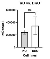
(9) The choice of ARMC1 and YY2 is unclear. What are the criteria for the selection?
ARMC1 was one of the top hits in a pilot RIP-seq experiment (IP versus input and IP versus IgG IP). In the actual RIP-seq experiment with DKO HAP1 cells instead of IgG IP as a negative control, we found ARMC1 as an enriched hit, although it was not among the top 5 hits. The results from the 2nd RIP-seq further confirmed the validity of ARMC1 as an L1TD1interacting transcript. YY2 was of potential biological relevance as an L1TD1 target due to the fact that it is a processed pseudogene originating from YY1 mRNA as a result of retrotransposition. This is mentioned on page 6 of the revised manuscript.
Response: Appreciated!
(10) (P16) L1 is the only protein-coding transposon that is active in humans. This is perhaps too generalized of a statement as written. Other examples are readily found in the literature.
Please clarify.
We will tone down this statement in the revised manuscript.
Response: Appreciated! To further clarify, the term "active" when it comes to transposable elements, has not been solidified. It can span "retrotransposition competent" to "transcripts can be recovered". There are quite a few reports of GAG transcripts and protein from various ERV/LTR subfamilies in various cells and tissues (in mouse and human at least), however whether they contribute to new insertions is actively researched.
(11) In both the abstract and last sentence in the discussion section (P17), embryogenesis is mentioned, but this is not addressed at all in the manuscript. Please refrain from implying normal biological functions based on the results of this study unless appropriate samples are used to support them.
Much of the published data on L1TD1 function are related to embryonic stem cells [3- 7].
Therefore, it is important to discuss our findings in the context of previous reports.
Response: It is well established that embryonic stem cells are not a perfect or direct proxies for the inner cell mass of embryos, as multiple reports have demonstrated transcriptomic, epigenetic, chromatin accessibility differences. The exact origin of ES cells is also considered controversial. We maintain that the distinction between embryos/embryogenesis and the results presented in the manuscript are not yet interchangeable. An important exception would be complex models of embryogenesis such as embryoids, (or synthetic/artificial embryo models that have been carefully been termed as such so as to not suggest direct implications to embryos). https://www.nature.com/articles/ncb2965
We have deleted the corresponding paragraph in the Discussion.
(12) Figure 3E: The format of Figures 1A and 3E are internally inconsistent. Please present similar data/images in a cohesive way throughout the manuscript. We show now consistent IF Figures in the revised manuscript.
Response: Thanks
Minor:
In general:
Still need checking for typos, mostly in Materials and Methods section; Please keep a consistent writing style throughout the whole manuscript. If you use L1 ORF1p, then please use L1 instead of LINE-1, or if you keep LINE-1 in your manuscript, then you should use LINE-1 ORF1p.
A lab member from the US checked again the Materials and Methods section for typos. We keep the short version L1 ORF1p.
(1) Intro:
- Is L1Td1 in mice and Humans? How "conserved" is it and does this suggest function? Murine and human L1TD1 proteins share 44% identity on the amino acid level and it was suggested that the corresponding genes were under positive selection during evolution with functions in transposon control and maintenance of pluripotency [8].
- Why HAP1? (Haploid?) The importance of this cell line is not clear.
HAP1 is a nearly haploid human cancer cell line derived from the KBM-7 chronic myelogenous leukemia (CML) cell line [9, 10]. Due to its haploidy is perfectly suited and widely used for loss-of-function screens and gene editing. After gene editing cells can be used in the nearly haploid or in the diploid state. We usually perform all experiments with diploid HAP1 cell lines. Importantly, in contrast to other human tumor cell lines, this cell line tolerates ablation of DNMT1. We have included a corresponding explanation in the revised manuscript on page 5, first paragraph.
- Global methylation status in DNMT1 KO? (Methylations near L1 insertions, for example?)
The HAP1 DNMT1 KO cell line with a 20 bp deletion in exon 4 used in our study was validated in the study by Smits et al. [11]. The authors report a significant reduction in overall DNA methylation. However, we are not aware of a DNA methylome study on this cell line. We show now data on the methylation of L1 elements in HAP1 cells and upon DNMT1 deletion in the revised manuscript in Suppl. Figure S1B.
Response: Looks great!
(2) Figure 1:
- Figure 1C. Why is LMNB used instead of Actin (Fig1D)?
We show now beta-actin as loading control in the revised manuscript.
- Figure 1G shows increased Caspase 3 in KO, while the matching sentence in the result section skips over this. It might be more accurate to mention this and suggest that the single KO has perhaps an intermediate phenotype (Figure 1F shows a slight but not significant trend).
We fully agree with the reviewer and have changed the sentence on page 6, 2nd paragraph accordingly.
- Would 96 hrs trend closer to significance? An interpretation is that L1TD1 loss could speed up this negative consequence.
We thank the reviewer for the suggestion. We have performed a time course experiment with 6 biological replicas for each time point up to 96 hours and found significant changes in the viability upon loss of DNMT1 and again significant reduction in viability upon additional loss of L1TD1 (shown in Figure 1F). These data suggest that as expected loss of DNMT1 leads to significant reduction viability and that additional ablation of L1TD1 further enhances this effect.
Response: Looks good!
- What are the "stringent conditions" used to remove non-specific binders and artifacts (negative control subtraction?)
Yes, we considered only hits from both analyses, L1TD1 IP in KO versus input and L1TD1 IP in KO versus L1TD1 IP in DKO. This is now explained in more detail in the revised manuscript on page 6, 3rd paragraph.
(3) Figure 2:
- Figure 2A is a bit too small to read when printed.
We have changed this in the revised manuscript.
- Since WT and DKO lack detectable L1TD1, would you expect any difference in RIP-Seq results between these two?
Due to the lack of DNMT1 and the resulting DNA hypomethylation, DKO cells are more similar to KO cells than WT cells with respect to the expressed transcripts.
- Legend says selected dots are in green (it appears blue to me). We have changed this in the revised manuscript.
- Would you recover L1 ORF1p and its binding partners in the KO? (Is the antibody specific in the absence of L1TD1 or can it recognize L1?) I noticed an increase in ORF1p in the KO in Figure 3C.
Thank you for the suggestion. Yes, L1 ORF1p shows slightly increased expression in the proteome analysis and we have marked the corresponding dot in the Volcano plot (Figure 3A).
- Should the figure panel reference near the (Rosspopoff & Trono) reference instead be Sup S1C as well? Otherwise, I don't think S1C is mentioned at all.
- What are the red vs. green dots in 2D? Can you highlight ERV and ALU with different colors?
We added the reference to Suppl. Figure S1C (now S3C) in the revised manuscript. In Figure 2D L1 elements are highlighted in green, ERV elements in yellow, and other associated transposon transcripts in red.
Response: Much better, thanks!
- Which L1 subfamily from Figure 2D is represented in the qRT-PCR in 2E "LINE-1"? Do the primers match a specific L1 subfamily? If so, which? We used primers specific for the human L1.2 subfamily.
- Pulling down SINE element transcripts makes some sense, as many insertions "borrow" L1 sequences for non-autonomous retro transposition, but can you speculate as to why ERVs are recovered? There should be essentially no overlap in sequence.
In the L1TD1 evolution paper [8], a potential link between L1TD1 and ERV elements was discussed:
"Alternatively, L1TD1 in sigmodonts could play a role in genome defense against another element active in these genomes. Indeed, the sigmodontine rodents have a highly active family of ERVs, the mysTR elements [46]. Expansion of this family preceded the death of L1s, but these elements are very active, with 3500 to 7000 speciesspecific insertions in the L1-extinct species examined [47]. This recent ERV amplification in Sigmodontinae contrasts with the megabats (where L1TD1 has been lost in many species); there are apparently no highly active DNA or RNA elements in megabats [48]. If L1TD1 can suppress retroelements other than L1s, this could explain why the gene is retained in sigmodontine rodents but not in megabats."
Furthermore, Jin et al. report the binding of L1TD1 to repetitive sequences in transcripts [12]. It is possible that some of these sequences are also present in ERV RNAs.
Response: Interesting, thanks for sharing
- Is S2B a screenshot? (the red underline).
No, it is a Powerpoint figure, and we have removed the red underline.
(4) Figure 3:
- Text refers to Figure 3B as a western blot. Figure 3B shows a volcano plot. This is likely 3C but would still be out of order (3A>3C>3B referencing). I think this error is repeated in the last result section.
- Figure and legends fail to mention what gene was used for ddCT method (actin, gapdh, etc.).
- In general, the supplemental legends feel underwritten and could benefit from additional explanations. (Main figures are appropriate but please double-check that all statistical tests have been mentioned correctly).
Thank you for pointing this out. We have corrected these errors in the revised manuscript.
(5) Discussion:
- Aluy connection is interesting. Is there an "Alu retrotransposition reporter assay" to test whether L1TD1 enhances this as well?
Thank you for the suggestion. There is indeed an Alu retrotransposition reporter assay reported be Dewannieux et al. [13]. The assay is based on a Neo selection marker. We have previously tested a Neo selection-based L1 retrotransposition reporter assay, but this system failed to properly work in HAP1 cells, therefore we switched to a blasticidin based L1 retrotransposition reporter assay. A corresponding blasticidin-based Alu retrotransposition reporter assay might be interesting for future studies (mentioned in the Discussion, page 11 paragraph 4 of the revised manuscript.
(6) Material and Methods :
- The number of typos in the materials and methods is too numerous to list. Instead, please refer to the next section that broadly describes the issues seen throughout the manuscript.
Writing style
(1) Keep a consistent style throughout the manuscript: for example, L1 or LINE-1 (also L1 ORF1p or LINE-1 ORF1p); per or "/"; knockout or knock-out; min or minute; 3 times or three times; media or medium. Additionally, as TE naming conventions are not uniform, it is important to maintain internal consistency so as to not accidentally establish an imprecise version.
(2) There's a period between "et al" and the comma, and "et al." should be italic.
(3) The authors should explain what the key jargon is when it is first used in the manuscript, such as "retrotransposon" and "retrotransposition".
(4) The authors should show the full spelling of some acronyms when they use it for the first time, such as RNA Immunoprecipitation (RIP).
(5) Use a space between numbers and alphabets, such as 5 μg. (6) 2.0 × 10⁵ cells, that's not an "x".
(7) Numbers in the reference section are lacking (hard to parse).
(8) In general, there are a significant number of typos in this draft which at times becomes distracting. For example, (P3) Introduction: Yet, co-option of TEs thorough (not thorough, it should be through) evolution has created so-called domesticated genes beneficial to the gene network in a wide range of organisms. Please carefully revise the entire manuscript for these minor issues that collectively erode the quality of this submission. Thank you for pointing out these mistakes. We have corrected them in the revised manuscript. A native speaker from our research group has carefully checked the paper. In summary, we have added Supplementary Figure S7C and have changed Figures 1C, 1E, 1F, 2A, 2D, 3A, 4B, S3A-D, S4B and S6A based on these comments.
Response: Thank you for taking these comments on board!
Author response:
The following is the authors’ response to the previous reviews.
Public Reviews:
Reviewer #1 (Public Review):
Summary:
The manuscript focuses on the role of the deubiquitinating enzyme UPS-50/USP8 in endosome maturation. The authors aimed to clarify how this enzyme drives the conversion of early endosomes into late endosomes. Overall, they did achieve their aims in shedding light on the precise mechanisms by which UPS-50/USP8 regulates endosome maturation. The results support their conclusions that UPS-50 acts by disassociating RABX-5 from early endosomes to deactivate RAB-5 and by recruiting SAND-1/Mon1 to activate RAB-7. This work is commendable and will have a significant impact on the field. The methods and data presented here will be useful to the community in advancing our understanding of endosome maturation and identifying potential therapeutic targets for diseases related to endosomal dysfunction. It is worth noting that further investigation is required to fully understand the complexities of endosome maturation. However, the findings presented in this manuscript provide a solid foundation for future studies.
We thank this reviewer for the instructive suggestions and encouragement.
Strengths:
The major strengths of this work lie in the well-designed experiments used to examine the effects of UPS-50 loss. The authors employed confocal imaging to obtain a picture of the aftermath of the USP-50 loss. Their findings indicated enlarged early endosomes and MVB-like structures in cells deficient in USP-50/USP8.
We thank this reviewer for the instructive suggestions and encouragement.
Weaknesses:
Specifically, there is a need for further investigation to accurately characterize the anomalous structures detected in the usp-50 mutant. Also, the correlation between the presence of these abnormal structures and ESCRT-0 is yet to be addressed, and the current working model needs to be revised to prevent any confusion between enlarged early endosomes and MVBs.
Excellent suggestions. USP8 has been identified as a protein associated with ESCRT components, which are crucial for endosomal membrane deformation and scission, leading to the formation of intraluminal vesicles (ILVs) within multivesicular bodies (MVBs). In usp-50 mutants, we observed a significant reduction in the punctate signals of HGRS-1::GFP and STAM-1 (Figure 1G and H; and Figure1-figure supplement 1B), indicating a disruption in ESCRT-0 complex localization (Author response image 1). Additionally, lysosomal structures are markedly reduced in these mutants. In contrast, we found that early endosomes, as marked by FYVE, RAB-5, RABEX5, and EEA1, are significantly enlarged in usp-50 mutants. Electron microscopy (EM) imaging further revealed an increase in large cellular vesicles containing various intraluminal structures. Given the reduction in lysosomal structures and the enlargement of early endosomes in usp-50 mutants, these enlarged vesicles are likely aberrant early endosomes rather than late endosomal or lysosomal structures. To address potential confusion, we have revised the manuscript according to the reviewer's comments and updated the model to accurately reflect these observations.
Reviewer #2 (Public Review):
Summary:
In this study, the authors study how the deubiquitinase USP8 regulates endosome maturation in C. elegans and mammalian cells. The authors have isolated USP8 mutant alleles in C. elegans and used multiple in vivo reporter lines to demonstrate the impact of USP8 loss-of-function on endosome morphology and maturation. They show that in USP8 mutant cells, the early endosomes and MVB-like structures are enlarged while the late endosomes and lysosomal compartments are reduced. They elucidate that USP8 interacts with Rabx5, a guanine nucleotide exchange factor (GEF) for Rab5, and show that USP8 likely targets specific lysine residue of Rabx5 to dissociate it from early endosomes. They also find that the localization of USP8 to early endosomes is disrupted in Rabx5 mutant cells. They observe that in both Rabx5 and USP8 mutant cells, the Rab7 GEF SAND-1 puncta which likely represents late endosomes are diminished, although Rabex5 is accumulated in USP8 mutant cells. The authors provide evidence that USP8 regulates endosomal maturation in a similar fashion in mammalian cells. Based on their observations they propose that USP8 dissociates Rabex5 from early endosomes and enhances the recruitment of SAND-1 to promote endosome maturation.
We thank this reviewer for the instructive suggestions and encouragement.
Strengths:
The major highlights of this study include the direct visualization of endosome dynamics in a living multi-cellular organism, C. elegans. The high-quality images provide clear in vivo evidence to support the main conclusions. The authors have generated valuable resources to study mechanisms involved in endosome dynamics regulation in both the worm and mammalian cells, which would benefit many members of the cell biology community. The work identifies a fascinating link between USP8 and the Rab5 guanine nucleotide exchange factor Rabx5, which expands the targets and modes of action of USP8. The findings make a solid contribution toward the understanding of how endosomal trafficking is controlled.
We thank this reviewer for the instructive suggestions and encouragement.
Weaknesses:
- The authors utilized multiple fluorescent protein reporters, including those generated by themselves, to label endosomal vesicles. Although these are routine and powerful tools for studying endosomal trafficking, these results cannot tell whether the endogenous proteins (Rab5, Rabex5, Rab7, etc.) are affected in the same fashion.
Good suggestion. Indeed, to test whether the endogenous proteins (Rab5, Rabex5, Rab7, etc.) are affected in the same fashion as fluorescent protein reporters, we supplemented our approach with the utilization of endogenous markers. These markers, including Rab5, RAB-5, Rabex5, RABX-5, and EEA1 for early endosomes, as well as RAB-7, Mon1a, and Mon1b for late endosomes, were instrumental in our investigations (refer to Figure 3, Figure 6, Figure 5-figure supplement 1, Figure 5-figure supplement 2, and Figure 6-figure supplement 1). Our comprehensive analysis, employing various methodologies such as tissue-specific fused proteins, CRISPR/Cas9 knock-in, and antibody staining, consistently highlights the critical role of USP8 in early-to-late endosome conversion.
- The authors clearly demonstrated a link between USP8 and Rabx5, and they showed that cells deficient in both factors displayed similar defects in late endosomes/lysosomes. However, the authors didn't confirm whether and/or to which extent USP8 regulates endosome maturation through Rabx5. Additional genetic and molecular evidence might be required to better support their working model.
Excellent point. To test whether USP-50 regulates endosome maturation through RABX-5, we performed additional genetic analyses. In rabx-5(null) mutant animals, the morphology of 2xFYVE-labeled early endosomes is comparable to that of wild-type controls (Figure 4H and I). Introducing the rabx-5(null) mutation into usp-50(xd413) backgrounds resulted in a significant suppression of the enlarged early endosome phenotype characteristic of usp-50(xd413) mutants (Figure 4H and I). These findings suggest that USP-50 may modulate the size of early endosomes through its interaction with RABX-5.
Reviewer #3 (Public Review):
Summary:
The authors were trying to elucidate the role of USP8 in the endocytic pathway. Using C. elegans epithelial cells as a model, they observed that when USP8 function is lost, the cells have a decreased number and size in lysosomes. Since USP8 was already known to be a protein linked to ESCRT components, they looked into what role USP8 might play in connecting lysosomes and multivesicular bodies (MVB). They observed fewer ESCRT-associated vesicles but an increased number of "abnormal" enlarged vesicles when USP8 function was lost. At this specific point, it's not clear what the objective of the authors was. What would have been their hypothesis addressing whether the reduced lysosomal structures in USP8 (-) animals were linked to MVB formation? Then they observed that the abnormally enlarged vesicles, marked by the PI3P biosensor YFP-2xFYVE, are bigger but in the same number in USP8 (-) compared to wild-type animals, suggesting homotypic fusion. They confirmed this result by knocking down USP8 in a human cell line, and they observed enlarged vesicles marked by YFP-2xFYVE as well. At this point, there is quite an important issue. The use of YFP-2xFYVE to detect early endosomes requires the transfection of the cells, which has already been demonstrated to produce differences in the distribution, number, and size of PI3P-positive vesicles (doi.org/10.1080/15548627.2017.1341465). The enlarged vesicles marked by YFP-2xFYVE would not necessarily be due to the loss of UPS8. In any case, it appears relatively clear that USP8 localizes to early endosomes, and the authors claim that this localization is mediated by Rabex-5 (or Rabx-5). They finally propose that USP8 dissociates Rabx-5 from early endosomes facilitating endosome maturation.
Weaknesses:
The weaknesses of this study are, on one side, that the results are almost exclusively dependent on the overexpression of fusion proteins. While useful in the field, this strategy does not represent the optimal way to dissect a cell biology issue. On the other side, the way the authors construct the rationale for each approximation is somehow difficult to follow. Finally, the use of two models, C. elegans and a mammalian cell line, which would strengthen the observations, contributes to the difficulty in reading the manuscript.
The findings are useful but do not clearly support the idea that USP8 mediates Rab5-Rab7 exchange and endosome maturation, In contrast, they appear to be incomplete and open new questions regarding the complexity of this process and the precise role of USP8 within it.
We thank this reviewer for the insightful comments. Fluorescence-fused proteins serve as potent tools for visualizing subcellular organelles both in vivo and in live settings. Specifically, in epidermal cells of worms, the tissue-specific expression of these fused proteins is indispensable for studying organelle dynamics within living organisms. This approach is necessitated by the inherent limitations of endogenously tagged proteins, whose fluorescence signals are often weak and unsuitable for live imaging or genetic screening purposes. Acknowledging concerns raised by the reviewer regarding potential alterations in organelle morphology due to overexpression of certain fused proteins, we supplemented our approach with the utilization of endogenous markers. These markers, including Rab5, RAB-5, Rabex5, RABX-5, and EEA1 for early endosomes, as well as RAB-7, Mon1a, and Mon1b for late endosomes, were instrumental in our investigations (refer to Figure 3, Figure 6, Figure 5-figure supplement 1, Figure 5-figure supplement 2, and Figure 6-figure supplement 1). Our comprehensive analysis, employing various methodologies such as tissue-specific fused proteins, CRISPR/Cas9 knock-in, and antibody staining, consistently highlights the critical role of USP8 in early-to-late endosome conversion. Specifically, we discovered that the recruitment of USP-50/USP8 to early endosomes is depending on Rabex5. However, instead of stabilizing Rabex5, the recruitment of USP-50/USP8 leads to its dissociation from endosomes, concomitantly facilitating the recruitment of the Rab7 GEF SAND-1/Mon1. In cells with loss-of-function mutations in usp-50/usp8, we observed enhanced RABX-5/Rabex5 signaling and mis-localization of SAND-1/Mon1 proteins from endosomes. Consequently, this disruption impairs endolysosomal trafficking, resulting in the accumulation of enlarged vesicles containing various intraluminal contents and rudimentary lysosomal structures.
Through an unbiased genetic screen, verified by cultured mammalian cell studies, we observed that loss-of-function mutations in usp-50/usp8 result in diminished lysosome/late endosomes. Electron microscopy (EM) analysis indicated that usp-50 mutation leads to abnormally enlarged vesicles containing various intraluminal structures in worm epidermal cells. USP8 is known to regulate the endocytic trafficking and stability of numerous transmembrane proteins. Given that lysosomes receive and degrade materials generated by endocytic pathways, we hypothesized that the abnormally enlarged vesicular structures observed in usp-50 or usp8 mutant cells correspond to the enlarged vesicles coated by early endosome markers. Indeed, in the absence of usp8/usp-50, the endosomal Rab5 signal is enhanced, while early endosomes are significantly enlarged. Given that Rab5 guanine nucleotide exchange factor (GEF), Rabex5, is essential for Rab5 activation, we further investigated its dynamics. Additional analyses conducted in both worm hypodermal cells and cultured mammalian cells revealed an increase of endosomal Rabex5 in response to usp8/usp-50 loss-of-function. Live imaging studies further demonstrated active recruitment of USP8 to newly formed Rab5-positive vesicles, aligning spatiotemporally with Rabex5 regulation. Through systematic exploration of putative USP-50 binding partners on early endosomes, we identified its interaction with Rabex5. Comprehensive genetics and biochemistry experiments demonstrated that USP8 acts through K323 site de-ubiquitination to dissociate Rabex5 from early endosomes and promotes the recruitment of the Rab7 GEF SAND-1/Mon1. In summary, our study began with an unbiased genetic screen and subsequent examination of established theories, leading to the formulation of our own hypothesis. Through multifaceted approaches, we unveiled a novel function of USP8 in early-to-late endosome conversion.
Recommendations for the authors:
Reviewer #1 (Recommendations For The Authors):
(1) Within Figures 1K-N, diverse anomalous structures were detected in the usp-50 mutant. Further scrutiny is needed to definitively characterize these structures, particularly as the images in Figures 1M and 1L exhibit notable similarities to lamellar bodies.
We thank the reviewer for the insightful question regarding the resemblance between the vesicles observed in our study and lamellar bodies (LBs). Lamellar bodies are specialized organelles involved in lipid storage and secretion1, prominently studied in keratinocytes of the skin and alveolar type II (ATII) epithelial cells in the lung2. These organelles contain not only lipids but also cell-type specific proteins and lytic enzymes. Due to their acidic pH and functional similarities, LBs are classified as lysosome-related organelles (LROs) or secretory lysosomes3,4. In usp-50 mutants, we observed a considerable number of abnormal vesicles, some of which contain threadlike membrane structures and exhibit morphological similarities to LBs (Figure 2O). However, further analysis with a comprehensive panel of lysosome-related markers demonstrated a significant reduction in lysosomal structures within these mutants. In contrast, vesicles marked by early endosome markers, such as FYVE, RAB-5, RABX-5, and EEA1, were notably enlarged. These results suggest that the enlarged vesicles observed in usp-50 mutants are more likely aberrant early endosomes rather than true lamellar bodies. We have revised the manuscript to reflect these findings and to clearly differentiate between these structures and lysosome-related organelles.
(2) The correlation between the presence of these abnormal structures and ESCRT-0 remains unaddressed, thus the assertion that UPS-50 regulates endolysosome trafficking in conjunction with ESCRT-0 lacks empirical support.
We thank the reviewer for the valuable suggestions. We apologize for any confusion and appreciate the opportunity to clarify our findings. The ESCRT machinery is essential for driving endosomal membrane deformation and scission, which leads to the formation of intraluminal vesicles (ILVs) within multivesicular bodies (MVBs). Recent research has shown that the absence of ESCRT components results in a reduction of ILVs in worm gut cells5. In wild type animals, the ESCRT-0 components HGRS-1 and STAM-1 display a distinct punctate distribution (Figure 1G and H). However, in usp-50 mutants, the punctate signals of HGRS-1::GFP and STAM-1::GFP are significantly reduced (Figure 1G and H; and Figure 1-figure supplement 1B), indicating a role for USP-50 in stabilizing the ESCRT-0 complex. Our TEM analysis revealed an accumulation of abnormally enlarged vesicles containing intraluminal structures in usp-50 mutants. When we examined a panel of early endosome and late endosome/lysosome markers, we found that early endosomes are significantly enlarged, while late endosomal/lysosomal structures are markedly reduced in these mutants. This suggests that the abnormal structures observed in usp-50 mutants are likely enlarged early endosomes rather than classical MVBs. To further investigate whether the reduction in ESCRT components contributes to the late endosome/lysosome defects, we analyzed stam-1 mutants. In these mutants, the size of RAB-7-coated vesicles was reduced (Author response image 1C), and the lysosomal marker LAAT-1 indicated a reduction in lysosomal structures (Author response image 1B). These results highlight the importance of the ESCRT complex in late endosome/lysosome formation. However, the morphology of early endosomes, as marked by 2xFYVE, remained similar to that of wild type in stam-1 mutants (Author response image 1A). Therefore, while reduced ESCRT-0 components may contribute to the late endosome/lysosome defects observed in usp-50 mutants, the enlargement of early endosomes in these mutants may involve additional mechanisms. We have revised the manuscript to incorporate these insights and to address the reviewer's comments more comprehensively.
Author response image 1.
(A) Confocal fluorescence images of hypodermis expressing YFP::2xFYVE to detect EEs in L4 stage animals in wild type and stam-1(ok406) mutants. Scale bar: 5 μm. (B) Confocal fluorescence images of hypodermal cell 7 (hyp7) expressing the LAAT-1::GFP marker to highlight lysosome structures in 3-day-old adult animals. Compared to wild type, LAAT-1::GFP signal is reduced in stam-1(ok406) animals. Scale bar, 5 μm. (C) The reduction of punctate endogenous GFP::RAB-7 signals in stam-1(ok406) animals. Scale bar: 10 μm.
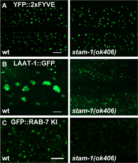
(3) Endosomal dysfunction typically leads to significant alterations in the spatial arrangement of marker proteins across distinct endosomes. In the manuscript, the authors examined the distribution and morphology of early endosomes, multivesicular bodies (MVBs), late endosomes, and lysosomes in a usp-50 deficient background primarily through single-channel confocal imaging. By employing two color images showing RAB-5 and RAB-7, in conjunction with HGRS-1, a more comprehensive picture of the aftermath of USP-50 loss can be obtained.
Good suggestions. We have conducted a double-labeling analysis to examine the distribution of RAB-5 and RAB-7 in conjunction with HGRS-1. In wild type animals, HGRS-1 exhibits a punctate distribution that is partially co-localized with both RAB-5 and RAB-7. In contrast, in usp-50 mutants, the punctate signal of HGRS-1 is significantly reduced, along with its co-localization with RAB-5 and RAB-7 (Author response image 2). These results suggest that, in the absence of USP-50, the stabilization of ESCRT-0 components on endosomes is compromised.
Author response image 2.
ESCRT-0 is adjacent to both early endosomes and late endosomes. (A) Confocal fluorescence images of wild-type and usp-50(xd413) hypodermis at L4 stage co-expressing HGRS-1::GFP (hgrs-1 promoter) and endogenous wrmScarlet::RAB-5. (B) HGRS-1 and RAB-5 puncta were analyzed to produce Manders overlap coefficient M1 (HGRS-1/RAB-5) and M2 (RAB-5/HGRS-1) (N=10). (C) Confocal fluorescence images of wild-type and usp-50(xd413) hypodermis at L4 stage co-expressing HGRS-1::GFP (hgrs-1 promoter) and endogenous wrmScarlet::RAB-7. (D) HGRS-1 and RAB-7 puncta were analyzed to produce Manders overlap coefficient M1 (HGRS-1/RAB-7) and M2 (RAB-7/HGRS-1) (N=10). Scale bar: 10 μm for (A) and (C).
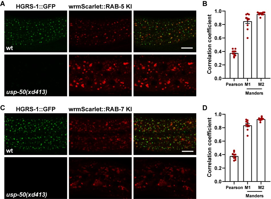
(4) The authors observed enlarged early endosomes in cells depleted of usp-50/usp8, along with enlarged MVB-like structures identified through TEM. The potential identity of these structures as the same organelle could be determined using CLEM.
We thank the reviewer for the valuable suggestion. Our TEM analysis identified a large number of abnormally enlarged vesicles with various intraluminal structures accumulated in usp-50 mutants. As the reviewer correctly noted, CLEM (correlative light and electron microscopy) would be an ideal approach to further characterize these structures. We have been attempting to implement CLEM in C. elegans for a few years. Given that CLEM relies on fluorescence markers, in this study we focused on two tagged proteins, RAB-5 and RABX-5, which show enlargement in their vesicles in usp-50 mutants. Unfortunately, we encountered significant challenges with this approach, as the GFP-tagged RAB-5 and RABX-5 signals did not survive the electron microscopy procedure. Attempts to align EM sections with residual GFP signaling yielded results that were not convincing. Consequently, we concentrated our analysis on a panel of molecular markers, including 2xFYVE, RAB-5, RABX-5, RAB-7, and LAAT-1. These markers consistently indicated that early endosomes are specifically enlarged in usp-50 mutants, while late endosomal/lysosomal structures are notably reduced. Thus, the abnormal structures identified in usp-50 mutants via TEM are likely to be enlarged early endosomes rather than the classical view of MVBs. We have revised the manuscript to reflect these findings and to clarify this point.
(5) The working model depicted in Figure 6 Y (right) requires revision, as it has the potential to mislead authors into mistaking enlarged early endosomes for multivesicular bodies (MVBs).
We thank the reviewer for the excellent suggestion. We have revised the model to clarify that it is the enlarged early endosomes, rather than MVBs, that are observed in usp-50 mutants.
Reviewer #2 (Recommendations For The Authors):
(1) Is there any change of Rabx5 protein level in USP8/USP50 mutant cells?
Good question. In the absence of usp-50/usp8, we indeed observed a noticeable increase in the signal of Rabex5 on endosomes. To determine whether usp-50/usp8 affects the protein level of Rabex5, we investigated the endogenous levels of RABX-5 using the RABX-5::GFP knock-in line. Compared to wild-type controls, we found an elevated protein level of RABX-5::GFP in the knock-in line (Author response image 3). This suggests that USP-50 may play a role in the destabilization of RABX-5/Rabex5 in vivo.
Author response image 3.
The endogenous RABX-5 protein level is increased in usp-50 mutants. (A) The RABX-5::GFP KI protein level is increased in usp-50(xd413). (B) Quantification of endogenous RABX-5::GFP protein level in wild type and usp-50(xd413) mutant animals.
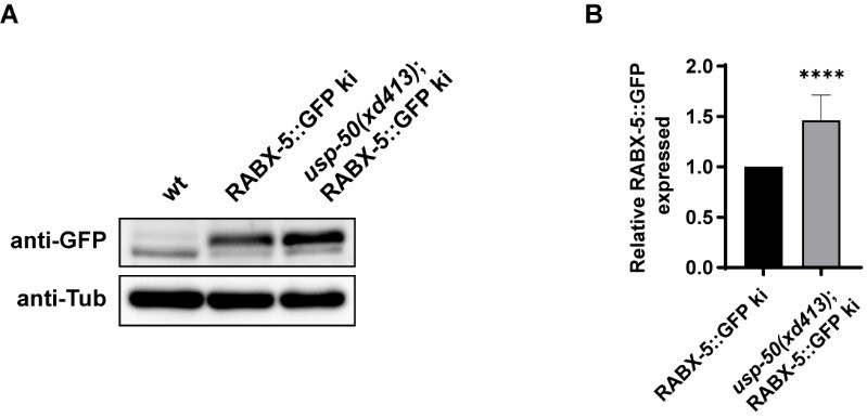
(2) It is interesting that "The rabx-5(null) animals are healthy and fertile and do not display obvious morphological or behavioral defects.", which seems contrary to its role in regulating USP8 localization and endosome maturation.
It has been previously documented that rabx-5 functions redundantly with rme-6, another RAB-5 GEF in C. elegans, to regulate RAB-5 localization in oocytes6. RNA interference (RNAi) targeting rabx-5 in a rme-6 mutant background results in synthetic lethality, whereas neither rabx-5 nor rme-6 single mutants are essential for worm viability. RME-6 co-localizes with clathrin-coated pits, while Rabex-5 is localized to early endosomes. Rabex-5 forms a stable complex with Rabaptin-5 and is part of a large EEA1-positive complex on early endosomes, whereas RME-6 does not interact with Rabaptin-5 (RABN-5) or EEA-1. These findings suggest that while RME-6 and RABX-5 may function redundantly, they likely play distinct roles in regulating intracellular trafficking processes. In the absence of RABX-5, USP-50 appears to lose its endosomal localization, although the size of the early endosome remains comparable to that of wild type. This observation contrasts with the phenotype associated with USP-50 loss-of-function, in which the early endosome is notably enlarged. These results suggest that residual USP-50 present in the endosomes is sufficient to maintain its role in the endocytic pathway. Conversely, the complete absence of USP-50 likely disrupts the transition of early endosomes to late endosomes, indicating a crucial role of USP-50 in this conversion process. It is also noteworthy that, although loss-of-function of rabx-5 does not result in obvious changes to early endosomes, increasing the gene expression level of rabx-5/Rabex-5 alone is sufficient to cause enlargement of early endosomes (Author response image 4) . Indeed, we observed that loss-of-function mutations in u_sp-50/usp_8 lead to abnormally enlarged early endosomes, accompanied by an enhanced signal of endosomal RABX-5. When the rabx-5(null) mutation was introduced into usp-50 mutant animals, the enlarged early endosome phenotype seen in usp-50 mutants was significantly suppressed (Figure 4H and I). This implies that maintaining a lower level of Rab5 GEF may be crucial for endolysosomal trafficking.
(3) Does Rabx5 mutation has any impact on early endosomes?
To address the question, we utilized the CRISPR/Cas9 technique to create a molecular null for rabx-5 (Figure 4E). In the rabx-5(null) mutant animals, we found that the 2xFYVE-labeled early endosomes are indistinguishable from wild type (Figure 4H and 4I). Given that r_abx-5_ functions redundantly with rme-6, another RAB-5 GEF in C. elegans, it is likely that the regulation of early endosome size involves a cooperative interaction between RABX-5 and RME-6.
(4) The authors observed a reduction of ESCRT-0 components in USP8 mutant cells, could this contribute to the late endosome/lysosome defects?
Good suggestion. In wild-type animals, the two ESCRT-0 components, HGRS-1 and STAM-1, exhibit a distinct punctate distribution (Figure 1G and H). However, in usp-50 mutants, the punctate signals of HGRS-1::GFP and STAM-1::GFP are significantly diminished (Figure 1G and H; and Figure 1-figure supplement 1B), which aligns with the role of USP-50 in stabilizing the ESCRT-0 complex. To investigate whether the reduction in ESCRT components might contribute to defects in late endosome/lysosome formation, we examined stam-1 mutants. In stam-1 mutants, we observed a reduction in the size of RAB-7-coated vesicles (Author response image 1). Further, when we introduced the lysosomal marker LAAT-1::GFP into stam-1 mutants, we found a substantial decrease in lysosomal structures compared to wild-type animals (Author response image 1). This suggests that the ESCRT complex is essential for proper late endosome/lysosome formation. In contrast, the morphology of early endosomes, as indicated by the 2xFYVE marker, appeared normal in stam-1 mutants, similar to wild-type animals (Author response image 1). This implies that while a reduction in ESCRT-0 components may contribute to the late endosome/lysosome defects observed in usp-50 mutants, the early endosome enlargement phenotype in _usp-5_0 mutants may involve additional mechanisms.
(5) Rabx5 is accumulated in USP8 mutant cells, I am very curious about the phenotype of USP8-Rabx5 double mutants. Could over-expression of Rabx5 (wild type or mutant forms) cause any defects?
Excellent suggestions. To address the question, we employed the CRISPR/Cas9 technique to create a molecular null for rabx-5 (Figure 4E). In the rabx-5(null) mutant animals, we observed that the punctate USP-50::GFP signal became diffusely distributed (Figure 4F and G). This suggests that rabx-5 is necessary for the endosomal localization of USP-50. Interestingly, in rabx-5(null) mutant animals, the 2xFYVE-labeled early endosomes appeared similar to those in wild-type animals (Figure 4H and I). When rabx-5(null) was introduced into usp-50 mutant animals, the enlarged early endosome phenotype observed in usp-50 was significantly suppressed (Figure 4H and I). This finding indicates that usp-50 indeed functions through rabx-5 to regulate early endosome size. Additionally, we constructed strains overexpressing either wild-type or K323R mutant RABX-5. Our results showed that overexpression of wild-type RABX-5 led to early endosome enlargement (as indicated by YFP::2xFYVE labeling) (Author response image 4A, B and D). In contrast, overexpression of the K323R mutant RABX-5 did not result in noticeable early endosome enlargement (Author response image 4A, C and D). Together, these data are in consistent with our model that USP-50 may regulate RABX-5 by deubiquitinating the K323 site.
Author response image 4.
(A-C) Over-expression wild type RABX-5 causes enlarged EEs (labeled by YFP::2xFYVE) while RABX-5(K323R) mutant form does not. (D) Quantification of the volume of individual YFP::2xFYVE vesicles. Data are presented as mean ± SEM. ****P<0.0001. ns, not significant. One-way ANOVA with Tukey’s test.
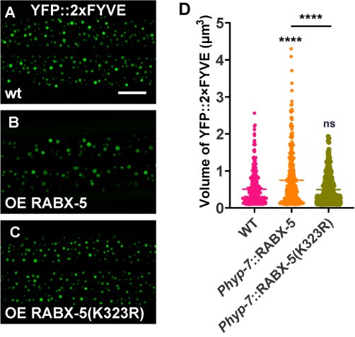
(6) Rabx5 could be ubiquitinated at K88 and K323, and Rabx5-K323R showed different activity when compared with the wild-type protein in USP8 mutant cells. Could the authors provide evidence that USP8 could remove the ubiquitin modification from K323 in Rabx5 protein?
We appreciate the reviewer's insightful suggestions. To explore the potential of USP-50 in removing ubiquitin modifications from lysine 323 on the RABX-5 protein, we undertook a series of experiments. Initially, we sought to determine whether USP-50 influences the ubiquitination level of RABX-5 in vivo. However, due to the low expression levels of USP-50, we encountered challenges in obtaining adequate amounts of USP-50 protein from worm lysates. To overcome this, we expressed USP-50::4xFLAG in HEK293 cells for subsequent affinity purification. Concurrently, we utilized anti-GFP agarose beads to purify RABX-5::GFP from worms expressing the rabx-5::gfp construct. We then incubated RABX-5::GFP with USP-50::4xFLAG for varying durations and performed immunoblotting with an anti-ubiquitin antibody. As shown in Author response image 5A, our results revealed a decrease in the ubiquitination level of RABX-5 in the presence of USP-50, suggesting that USP-50 directly deubiquitinates RABX-5. Previous studies have indicated that only a minor fraction of recombinant RABX-5 undergoes ubiquitination in HeLa cells, which is believed to have functional significance7. Our findings are consistent with this observation, as only a small fraction of RABX-5 in worms is ubiquitinated. Rabex-5 is known to interact with both K63- and K48-linked poly-ubiquitin chains. To further elucidate whether USP-50 specifically targets K48 or K63-linked ubiquitination at the K323 site of RABX-5, we incubated various HA-tagged ubiquitin mutants with either wild-type or K323R mutant RABX-5 protein. Our results indicated that the K323R mutation reduces K63-linked ubiquitination of RABX-5 (Author response image 5). This experiment was repeated multiple times with consistent results. Additionally, while overexpression of wild-type RABX-5 led to an enlargement of early endosomes, as evidenced by YFP::2xFYVE labeling, overexpression of the K323R mutant did not produce a noticeable effect on endosome size (Author response image 4). Collectively, this finding indicates that RABX-5 is subject to ubiquitin modification in vivo and that USP-50 plays a significant role in regulating this modification at the K323 site.
Author response image 5.
(A) RABX-5::GFP protein was purified from worm lysates using anti-GFP antibody. FLAG-tagged USP-50 was purified from HEK293T cells using anti-FLAG antibody. Purified RABX-5::GFP was incubated with USP-50::4FLAG for indicated times (0, 15, 30, 60 mins), followed by immunoblotting using antibody against ubiquitin, FLAG or GFP. In the presence of USP-50::4xFLAG, the ubiquitination level of RABX-5::GFP is decreased. (B) Quantification of RABX-5::GFP ubiquitination level from three independent experiments. (C) HEK293T cells were transfected with HA-Ub or indicated mutants and 4xFLAG tagged RABX-5 or RABX-5 K323R mutant for 48h. The cells were subjected to pull down using the FLAG beads, followed by immunoblotting using antibody against HA or Flag.
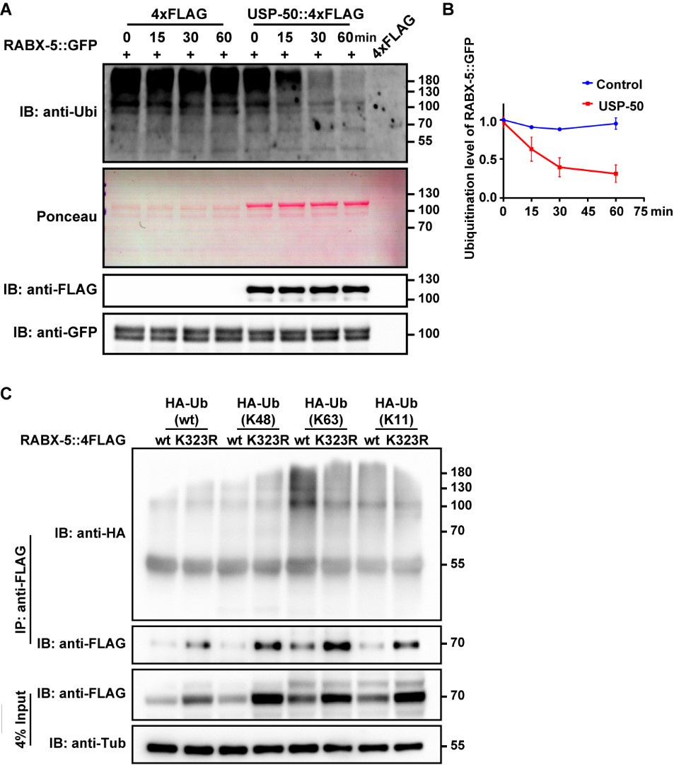
(7) The authors described "the almost identical phenotype of usp-50/usp8 and sand-1/Mon1 mutants", found protein-protein interaction between USP8 and sand-1, and showed that sand1-GFP signal is diminished in USP8 mutant cells. These observations fit with the possibility that USP8 regulates the stability of sand-1 to promote endosomal maturation. Could this be tested and integrated into the current model?
are grateful for the insightful comments provided by the reviewer. Rab5, known to be activated by Rabex-5, plays a crucial role in the homotypic fusion of early endosomes. Rab5 effectors also include the Rab7 GEF SAND-1/Mon1–Ccz1 complex. Rab7 activation by SAND-1/Mon1-Ccz1 complex is essential for the biogenesis and positioning of late endosomes (LEs) and lysosomes, and for the fusion of endosomes and autophagosomes with lysosomes. The Mon1-Ccz1 complex is able to interact with Rabex5, causing dissociation of Rabex5 from the membrane, which probably terminates the positive feedback loop of Rab5 activation and then promotes the recruitment and activation of Rab7 on endosomes. In our study, we identified an interaction between USP-50 and the Rab5 GEF, RABX-5. In the absence of USP-50, we observed an increased endosomal localization of RABX-5 and the formation of abnormally enlarged early endosomes. This phenotype is reminiscent of that seen in sand-1 loss-of-function mutants, which also exhibit enlarged early endosomes and a concomitant reduction in late endosomes/lysosomes. Notably, USP-50 also interacts with SAND-1, suggesting a potential role in regulating its localization. We could propose several models to elucidate how USP-50 might influence SAND-1 localization, including:
(1) USP-50 may stabilize SAND-1 through direct de-ubiquitination.
(2) In the absence of USP-50, the sustained presence of RABX-5 could lead to continuous Rab5 activation, which might hinder or delay the recruitment of SAND-1.
(3) USP-50 could facilitate SAND-1 recruitment by promoting the dissociation of RABX-5.
We are actively investigating these models in our laboratory. Due to space constraints, a more detailed exploration of how USP-50 regulates SAND-1 stability will be presented in a separate publication.
References:
(1) Schmitz, G., and Müller, G. (1991). Structure and function of lamellar bodies, lipid-protein complexes involved in storage and secretion of cellular lipids. J Lipid Res 32, 1539-1570.
(2) Dietl, P., and Frick, M. (2021). Channels and Transporters of the Pulmonary Lamellar Body in Health and Disease. Cells-Basel 11. https://doi.org/10.3390/cells11010045.
(3) Raposo, G., Marks, M.S., and Cutler, D.F. (2007). Lysosome-related organelles: driving post-Golgi compartments into specialisation. Current opinion in cell biology 19, 394-401. https://doi.org/10.1016/j.ceb.2007.05.001.
(4) Weaver, T.E., Na, C.L., and Stahlman, M. (2002). Biogenesis of lamellar bodies, lysosome-related organelles involved in storage and secretion of pulmonary surfactant. Semin Cell Dev Biol 13, 263-270. https://doi.org/10.1016/s1084952102000551.
(5) Ott, D.P., Desai, S., Solinger, J.A., Kaech, A., and Spang, A. (2024). Coordination between ESCRT function and Rab conversion during endosome maturation. bioRxiv, 2024.2005.2014.594104. https://doi.org/10.1101/2024.05.14.594104.
(6) Sato, M., Sato, K., Fonarev, P., Huang, C.J., Liou, W., and Grant, B.D. (2005). Caenorhabditis elegans RME-6 is a novel regulator of RAB-5 at the clathrin-coated pit. Nature cell biology 7, 559-569. https://doi.org/10.1038/ncb1261.
(7) Mattera, R., Tsai, Y.C., Weissman, A.M., and Bonifacino, J.S. (2006). The Rab5 guanine nucleotide exchange factor Rabex-5 binds ubiquitin (Ub) and functions as a Ub ligase through an atypical Ub-interacting motif and a zinc finger domain. The Journal of biological chemistry 281, 6874-6883. https://doi.org/10.1074/jbc.M509939200.
Author response:
The following is the authors’ response to the previous reviews.
Reviewer #1 (Public Review):
Comments on revisions)
The authors have done a good job at revising the manuscript to put this work into the context of earlier work on brainstem central pattern generators.
Thank you.
I still believe the case for the method is not as convincing as it would have been if the method had been validated first on oscillations produced by a known CPG model. Why would the inference of synaptic types from the model CPG voltage oscillations be predetermined? Such inverse problems are quite complicated and their solution is often not unique or sufficiently constrained. Recovering synaptic weights (or CPG parameters) from limited observations of a highly nonlinear system is not warranted (Gutenkunst et al., Universally sloppy parameter sensitivities in systems biology models, PLoS Comp. Biol. 2007; www.doi.org/10.1371/journal.pcbi.0030189) especially when using surrogate biological models like Hodgkin-Huxley models.
The model of the CPG is irrelevant for such a test of validity because what we reconstruct are postsynaptic conductances of an individual neuron. The network creates a periodic input to this neuron and thus forms a periodic pattern of excitatory and inhibitory conductances. The nature of this input, whether autonomously generated or created artificially (say by periodic optogenetic stimulation), is generally not important. To illustrate this, we used a one-compartment conductance-based (Hodgkin-Huxley style) model neuron incorporating a certain common set of channels (fast sodium (I<sub>NaF</sub>), potassium delayed rectifier (I<sub>Kdr</sub>), persistent sodium (I<sub>NaP</sub>), calcium-dependent potassium (I<sub>KCa</sub>), and cationic non-specific current (I<sub>CAN</sub>)), as well as excitatory and inhibitory synaptic channels whose conductances were implemented as predefined periodic functions. The test suggested by the reviewer would be to implement a current-step protocol similar to the experiments and apply our technique to see if the reconstructed conductance profiles match those predefined functions. Below we show the reconstruction steps for the following arbitrarily chosen pattern:
𝑔<sub>𝐸𝑋𝐶</sub>(𝑡) /𝑔<sub>𝐿𝐸𝐴𝐾</sub> = 0.1(1 + sin(π𝑡)) and 𝑔<sub>𝐼𝑁𝐻</sub>(𝑡)/𝑔<sub>𝐿𝐸𝐴𝐾</sub> = 0.1 (1 + cos(π𝑡)). Author response image 1 below shows the baseline activity of this model neuron in the absence of the injected current.
Author response image 1.
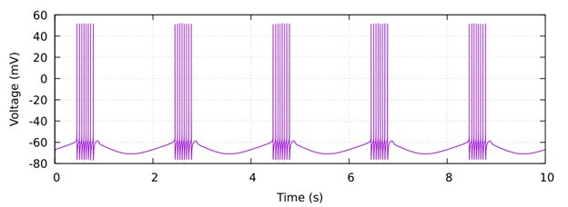
Then we applied a current-step protocol with four steps producing different levels of hyperpolarization and applied our method by calculating the total conductance using linear regression (see the current-voltage plots below) and then decomposing it into the excitatory and inhibitory components.
Author response image 2.
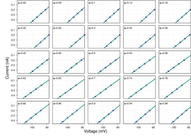
As one can see, the reconstructed conductances in Author response image 3 below are nearly identical to their theoretical profiles. This is not surprising because all voltage-dependent currents in the model neuron were inactive in the range of voltages matching our experimental conditions. Therefore, the model could be reduced to just the leak current, synaptic currents and the injected current, which matches precisely the model we used in our manuscript.
Author response image 3.
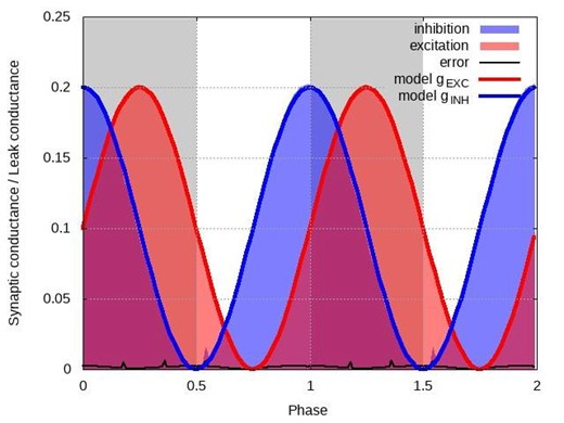
In p.2, the edited section refers to the interspike interval being much smaller than the period of the network. More important is to mention the relationship between the decay time of inhibitory synapses and the period of the network.
This interpretation misunderstands the focus of our method. The edited sections (including in the theory section of Results) highlight the conditions under which the capacitive current becomes negligible, emphasizing that the membrane time constant must be much smaller than the network oscillation period. This separation of time scales ensures that the membrane potential adjusts quickly to changes in postsynaptic conductance, rendering the capacitive current insignificant over the network’s rhythm. In contrast, the synaptic decay time governs how presynaptic inputs are transduced into postsynaptic conductances—a process relevant to understanding synaptic dynamics but not directly tied to our method’s core objective. Our approach reconstructs postsynaptic conductances from intracellular recordings, not presynaptic spike trains. While interpreting these conductance profiles in terms of specific synaptic connections would indeed involve synaptic decay dynamics, such an analysis exceeds the scope of our paper. Thus, the condition emphasized in the edited sections—concerning the membrane time constant and network period—is the critical one for our method’s applicability, and the synaptic decay time, while relevant to broader synaptic modeling, does not undermine our conclusions.
We have added the requirement for a much smaller membrane time constant in the Introduction on page 2. The Results theory section already incorporates an extensive discussion of this requirement.
Comments from the editors:
We apologize for the delay in coming to this decision, but there was quite a bit of post-review discussion that needed to be resolved. There are two issues that the reviewers agree should be addressed. They remain unconvinced that the simplifying assumptions of the approach are valid. 1) The main issue with the phase argument is that the biological synaptic conductance depends on time and not on the phase of the respiratory cycle as mentioned in the first round of reviews. The approximation g(t)=g(phase) seems to be far too simple to be biologically realistic.
As we elaborate below, time and phase are fundamentally and mathematically equivalent representations of the same underlying dynamics in a periodic system, and thus, a phase-based representation—where conductances are expressed as functions of the cycle’s phase—is a justified and effective approach for capturing their behavior. We have added this explanation to the theory section of Results. Below are the bases for our assertion.
In a periodic system, such as the respiratory CPG, the system’s behavior repeats at regular intervals, defined by a period T. For the respiratory cycle in our experimental preparation, this period is approximately 3–4 seconds, encompassing phases like inspiration, post-inspiration, and expiration. In such systems:
Time (t) is a continuous variable that progresses linearly.
Phase (φ) represents the position within one cycle, typically normalized between 0 and 1 (or 0 to 2π in some contexts). It can be mathematically related to time via: φ(t) = (t mod T)/T, where (t mod T) is the time elapsed within the current cycle.
Because the system is periodic, any variable that repeats with period T—such as synaptic conductance in a rhythmically active network—can be expressed as a function of either time or phase. Specifically, if g(t) is periodic with period T, then g(t) = g(t+T). This periodicity allows us to redefine g(t) in terms of phase: g(t) = g(φ(t)), where φ(t) maps time onto a repeating cycle. Thus, in a periodic system, time and phase are fundamentally equivalent representations of the same underlying dynamics. Saying that synaptic conductance depends on phase is mathematically equivalent to saying it depends on time in a periodic manner.
In a rhythmically active network like the respiratory central pattern generator (CPG), the synaptic conductances, regardless of the specific mechanisms by which they are formed, exhibit periodicity that matches the network’s oscillatory cycle. This occurs because the conductances are driven by the repetitive activity of presynaptic neurons, which are synchronized to the network’s overall rhythm. As a result, the synaptic conductances vary with the same period as the network, making a phase-based representation—where conductances are expressed as functions of the cycle’s phase—a justified and effective approach for capturing their behavior. In our study, we utilized the in situ arterially perfused brainstem-spinal cord preparation from mature rats, which is known to produce a highly periodic respiratory rhythm. To ensure the consistency of this periodicity, we carefully selected recordings where the coefficient of variation of the respiratory cycle period was less than 10%, as outlined in our methods. This strict selection criterion confirms the stability and regularity of the rhythm, supporting the validity of using a phase representation to analyze the synaptic conductances.
(2) Figure S1 is problematic. First, the currents injected appear to be infinitesimally small.
There was a typo in the current units, which should be nA and not pA, as evident from the injected current–membrane potential plots in Figure 1B. Figure S1 has been corrected.
Second, the input resistance is completely independent of voltage, as though there was little or no contribution from hyperpolarization activated currents, which would be surprising.
While hyperpolarization-activated currents are indeed present in many neuronal types and could theoretically affect input resistance, our data consistently show linear I-V relationships across the voltage range tested (-60 to -100 mV) for the neurons analyzed (see Figure S1 and Author response image 4-9 below). This linearity suggests that, under our experimental conditions, the contribution of voltage-dependent currents, such as h-currents, is negligible within this range.
Additionally, we now indicate in the manuscript in the theory section of Results how the presence of significant hyperpolarization-activated h-currents would impact our synaptic conductance reconstruction method. In current-clamp recordings, non-linearity from h-currents could introduce voltage-dependent changes in total conductance unrelated to synaptic inputs, potentially skewing the reconstruction. However, this concern does not apply to voltage-clamp recordings, where the membrane potential is held constant, eliminating contributions from voltage-dependent intrinsic currents. As strong evidence of the minimal influence of h-currents, we directly compared synaptic conductance reconstructions using both current-clamp and voltage-clamp protocols in a subset of neurons. The results from these two approaches were highly consistent, indicating that h-currents do not significantly affect our findings. This robustness across experimental methods reinforces the reliability of our conclusions.
Together, the linear I-V relationships and the agreement between current- and voltage-clamp reconstructions provide compelling evidence that our method accurately captures synaptic conductances without interference from h-currents.
Typical examples of I-V relationships for each respiratory neuron firing phenotype:
Author response image 4.
ramp-I
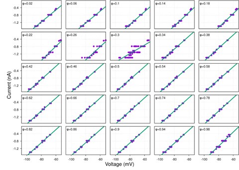
Author response image 5.
pre-I/I
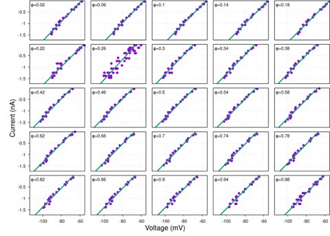
Author response image 6.
post-I
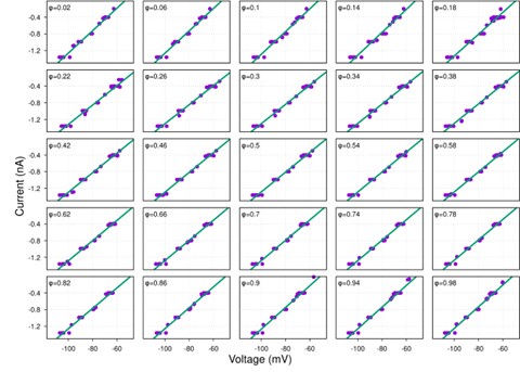
Author response image 7.
aug-E
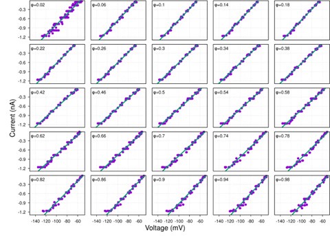
Author response image 8.
early-I
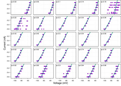
Author response image 9.
late-I
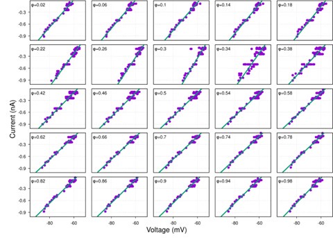
Author Response
The following is the authors’ response to the previous reviews.
We thank the reviewers for truly valuable advice and comments. We have made multiple corrections and revisions to the original pre-print accordingly per the following comments:
- Pro1153Leu is extremely common in the general population (allele frequency in gnomAD is 0.5). Further discussion is warranted to justify the possibility that this variant contributes to a phenotype documented in 1.5-3% of the population. Is it possible that this variant is tagging other rare SNPs in the COL11A1 locus, and could any of the existing exome sequencing data be mined for rare nonsynonymous variants?
One possible avenue for future work is to return to any existing exome sequencing data to query for rare variants at the COL11A1 locus. This should be possible for the USA MO case-control cohort. Any rare nonsynonymous variants identified should then be subjected to mutational burden testing, ideally after functional testing to diminish any noise introduced by rare benign variants in both cases and controls. If there is a significant association of rare variation in AIS cases, then they should consider returning to the other cohorts for targeted COL11A1 gene sequencing or whole exome sequencing (whichever approach is easier/less expensive) to demonstrate replication of the association.
Response: Regarding the genetic association of the common COL11A1 variant rs3753841 (p.(Pro1335Leu)), we do not propose that it is the sole risk variant contributing to the association signal we detected and have clarified this in the manuscript. We concluded that it was worthy of functional testing for reasons described here. Although there were several common variants in the discovery GWAS within and around COL11A1, none were significantly associated with AIS and none were in linkage disequilibrium (R2>0.6) with the top SNP rs3753841. We next reviewed rare (MAF<=0.01) coding variants within the COL11A1 LD region of the associated SNP (rs3753841) in 625 available exomes representing 46% of the 1,358 cases from the discovery cohort. The LD block was defined using Haploview based on the 1KG_CEU population. Within the ~41 KB LD region (chr1:103365089- 103406616, GRCh37) we found three rare missense mutations in 6 unrelated individuals, Table below. Two of them (NM_080629.2: c.G4093A:p.A1365T; NM_080629.2:c.G3394A:p.G1132S), from two individuals, are predicted to be deleterious based on CADD and GERP scores and are plausible AIS risk candidates. At this rate we could expect to find only 4-5 individuals with linked rare coding variants in the total cohort of 1,358 which collectively are unlikely to explain the overall association signal we detected. Of course, there also could be deep intronic variants contributing to the association that we would not detect by our methods. However, given this scenario, the relatively high predicted deleteriousness of rs3753841 (CADD= 25.7; GERP=5.75), and its occurrence in a GlyX-Y triplet repeat, we hypothesized that this variant itself could be a risk allele worthy of further investigation.
Author response table 1.
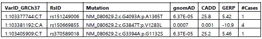
We also appreciate the reviewer’s suggestion to perform a rare variant burden analysis of COL11A1. We did conduct pilot gene-based analysis in 4534 European ancestry exomes including 797 of our own AIS cases and 3737 controls and tested the burden of rare variants in COL11A1. SKATO P value was not significant (COL11A1_P=0.18), but this could due to lack of power and/or background from rare benign variants that could be screened out using the functional testing we have developed.
- COL11A1 p.Pro1335Leu is pursued as a direct candidate susceptibility locus, but the functional validation involves both: (a) a complementation assay in mouse GPCs, Figure 5; and (b) cultured rib cartilage cells from Col11a1-Ad5 Cre mice (Figure 4). Please address the following:
2A. Is Pro1335Leu a loss of function, gain of function, or dominant negative variant? Further rationale for modeling this change in a Col11a1 loss of function cell line would be helpful.
Response: Regarding functional testing, by knockdown/knockout cell culture experiments, we showed for the first time that Col11a1 negatively regulates Mmp3 expression in cartilage chondrocytes, an AIS-relevant tissue. We then tested the effect of overexpressing the human wt or variant COL11A1 by lentiviral transduction in SV40-transformed chondrocyte cultures. We deleted endogenous mouse Col11a1 by Cre recombination to remove the background of its strong suppressive effects on Mmp3 expression. We acknowledge that Col11a1 missense mutations could confer gain of function or dominant negative effects that would not be revealed in this assay. However as indicated in our original manuscript we have noted that spinal deformity is described in the cho/cho mouse, a Col11a1 loss of function mutant. We also note the recent publication by Rebello et al. showing that missense mutations in Col11a2 associated with congenital scoliosis fail to rescue a vertebral malformation phenotype in a zebrafish col11a2 KO line. Although the connection between AIS and vertebral malformations is not altogether clear, we surmise that loss of the components of collagen type XI disrupt spinal development. in vivo experiments in vertebrate model systems are needed to fully establish the consequences and genetic mechanisms by which COL11A1 variants contribute to an AIS phenotype.
2B. Expression appears to be augmented compared WT in Fig 5B, but there is no direct comparison of WT with variant.
Response: Expression of the mutant (from the lentiviral expression vector) is increased compared to mutant. We observed this effect in repeated experiments. Sequencing confirmed that the mutant and wildtype constructs differed only at the position of the rs3753841 SNP. At this time, we cannot explain the difference in expression levels. Nonetheless, even when the variant COL11A1 is relatively overexpressed it fails to suppress MMP3 expression as observed for the wildtype form.
2C. How do the authors know that their complementation data in Figure 5 are specific? Repetition of this experiment with an alternative common nonsynonymous variant in COL11A1 (such as rs1676486) would be helpful as a comparison with the expectation that it would be similar to WT.
Response: We agree that testing an allelic series throughout COL11A1 could be informative, but we have shifted our resources toward in vivo experiments that we believe will ultimately be more informative for deciphering the mechanistic role of COL11A1 in MMP3 regulation and spine deformity.
2D. The y-axes of histograms in panel A need attention and clarification. What is meant by power? Do you mean fold change?
Response: Power is directly comparable to fold change but allows comparison of absolute expression levels between different genes.
2E. Figure 5: how many technical and biological replicates? Confirm that these are stated throughout the figures.
Response: Thank you for pointing out this oversight. This information has been added throughout.
- Figure 2: What does the gross anatomy of the IVD look like? Could the authors address this by showing an H&E of an adjacent section of the Fig. 2 A panels?
Response: Panel 2 shows H&E staining. Perhaps the reviewer is referring to the WT and Pax1 KO images in Figure 3? We have now added H&E staining of WT and Pax1 KO IVD as supplemental Figure 3E to clarify the IVD anatomy.
- Page 9: "Cells within the IVD were negative for Pax1 staining ..." There seems to be specific PAX1 expression in many cells within the IVD, which is concerning if this is indeed a supposed null allele of Pax1. This data seems to support that the allele is not null.
Response: We have now added updated images for the COL11A1 and PAX1 staining to include negative controls in which we omitted primary antibodies. As can be seen, there is faint autofluorescence in the PAX1 negative control that appears to explain the “specific staining” referred to by the reviewer. These images confirm that the allele is truly a null.
- There is currently a lack of evidence supporting the claim that "Col11a1 is positively regulated by Pax1 in mouse spine and tail". Therefore, it is necessary to conduct further research to determine the direct regulatory role of Pax1 on Col11a1.
Response: We agree with the reviewer and have clarified that Pax1 may have either a direct or indirect role in Col11a1 regulation.
- There is no data linking loss of COL11A1 function and spine defects in the mouse model. Furthermore, due to the absence of P1335L point mutant mice, it cannot be confirmed whether P1335L can actually cause AIS, and the pathogenicity of this mutation cannot be directly verified. These limitations need to be clearly stated and discussed. A Col11a1 mouse mutant called chondroysplasia (cho), was shown to be perinatal lethal with severe endochondral defects (https://pubmed.ncbi.nlm.nih.gov/4100752/). This information may help contextualize this study.
Response: We partially agree with the reviewer. Spine defects are reported in the cho mouse (for example, please see reference 36 Hafez et al). We appreciate the suggestion to cite the original Seegmiller et al 1971 reference and have added it to the manuscript.
- A recent article (PMID37462524) reported mutations in COL11A2 associated with AIS and functionally tested in zebrafish. That study should be cited and discussed as it is directly relevant for this manuscript.
Response: We agree with the reviewer that this study provides important information supporting loss of function I type XI collagen in spinal deformity. Language to this effect has been added to the manuscript and this study is now cited in the paper.
- Please reconcile the following result on page 10 of the results: "Interestingly, the AISassociated gene Adgrg6 was amongst the most significantly dysregulated genes in the RNA-seq analysis (Figure 3c). By qRT-PCR analysis, expression of Col11a1, Adgrg6, and Sox6 were significantly reduced in female and male Pax1-/- mice compared to wild-type mice (Figure 3d-g)." In Figure 3f, the downregulation of Adgrg6 appears to be modest so how can it possibly be highlighted as one of the most significantly downregulated transcripts in the RNAseq data?
Response: By “significant” we were referring to the P-value significance in RNAseq analysis, not in absolute change in expression. This language was clearly confusing, and we have removed it from the manuscript.
- It is incorrect to refer to the primary cell culture work as growth plate chondrocytes (GPCs), instead, these are primary costal chondrocyte cultures. These primary cultures have a mixture of chondrocytes at differing levels of differentiation, which may change differentiation status during the culturing on plastic. In sum, these cells are at best chondrocytes, and not specifically growth plate chondrocytes. This needs to be corrected in the abstract and throughout the manuscript. Moreover, on page 11 these cells are referred to as costal cartilage, which is confusing to the reader.
Response: Thank you for pointing out these inconsistencies. We have changed the manuscript to say “costal chondrocytes” throughout.
Minor points
- On 10 of the Results: "These data support a mechanistic link between Pax1 and Col11a1, and the AIS-associated genes Gpr126 and Sox6, in affected tissue of the developing tail." qRT-PCR validation of Sox6, although significant, appears to be very modestly downregulated in KO. Please soften this statement in the text.
Response: We have softened this statement.
- Have you got any information about how the immortalized (SV40) costal cartilage affected chondrogenic differentiation? The expression of SV40 seemed to stimulate Mmp13 expression. Do these cells still make cartilage nodules? Some feedback on this process and how it affects the nature of the culture what be appreciated.
Response: The “+ or –“ in Figure 5 refers to Ad5-cre. Each experiment was performed in SV40-immortalized costal chondrocytes. We have removed SV40 from the figure and have clarified the legend to say “qRT-PCR of human COL11A1 and endogenous mouse Mmp3 in SV40 immortalized mouse costal chondrocytes transduced with the lentiviral vector only (lanes 1,2), human WT COL11A1 (lane 3), or COL11A1P1335L. Otherwise we absolutely agree that understanding Mmp13 regulation during chondrocyte differentiation is important. We plan to study this using in vivo systems.
- Figure 1: is the average Odds ratio, can this be stated in the figure legend?
Response: We are not sure what is being asked here. The “combined odds ratio” is calculated as a weighted average of the log of the odds.
- A more consistent use of established nomenclature for mouse versus human genes and proteins is needed.
Human:GENE/PROTEIN Mouse: Gene/PROTEIN
Response: Thank you for pointing this out. The nomenclature has been corrected throughtout the manuscript.
- There is no Figure 5c, but a reference to results in the main text. Please reconcile. -There is no Figure 5-figure supplement 5a, but there is a reference to it in the main text. Please reconcile.
Response: Figure references have been corrected.
- Please indicate dilutions of all antibodies used when listed in the methods.
Response: Antibody dilutions have been added where missing.
- On page 25, there is a partial sentence missing information in the Histologic methods; "#S36964 Invitrogen, CA, USA)). All images were taken..."
Response: We apologize for the error. It has been removed.
- Table 1: please define all acronyms, including cohort names.
Response: We apologize for the oversight. The legend to the Table has been updated with definitions of all acronyms.
- Figure 2: Indicate that blue staining is DAPI in panel B. Clarify that "-ab" as an abbreviation is primary antibody negative.
Response: A color code for DAPI and COL11A! staining has been added and “-ab” is now defined.
- Page 4: ADGRG6 (also known as GPR126)...the authors set this up for ADGRG6 but then use GPR126 in the manuscript, which is confusing. For clarity, please use the gene name Adgrg6 consistently, rather than alternating with Gpr126.
Response: Thank you for pointing this out. GPR126 has now been changed to ADGRG6 thoughout the manuscript.
- REF 4: Richards, B.S., Sucato, D.J., Johnston C.E. Scoliosis, (Elsevier, 2020). Is this a book, can you provide more clarity in the Reference listing?
Response: Thank you for pointing this out. This reference has been corrected.
- While isolation was addressed, the methods for culturing Rat cartilage endplate and costal chondrocytes are poorly described and should be given more text.
Response: Details about the cartilage endplate and costal chondrocyte isolation and culture have been added to the Methods.
- Page 11: 1st paragraph, last sentence "These results suggest that Mmp3 expression"... this sentence needs attention. As written, I am not clear what the authors are trying to say.
Response: This sentence has been clarified and now reads “These results suggest that Mmp3 expression is negatively regulated by Col11a1 in mouse costal chondrocytes.”
- Page 13: line 4 from the bottom, "ECM-clearing"? This is confusing do you mean ECM degrading?
Response: Yes and thank you. We have changed to “ECM-degrading”.
- Please use version numbers for RefSeq IDs: e.g. NM_080629.3 instead of NM_080629
Response: This change has been made in the revised manuscript.
- It would be helpful for readers if the ethnicity of the discovery case cohort was clearly stated as European ancestry in the Results main text.
Response: “European ancestry” has been added at first description of the discovery cohort in the manuscript.
- Avoid using the term "mutation" and use "variant" instead.
Response: Thank you for pointing this out. “Variant” is now used throughout the manuscript.
- Define error bars for all bar charts throughout and include individual data points overlaid onto bars.
Response: Thank you. Error bars are now clarified in the Figure legends.
Author response:
The following is the authors’ response to the previous reviews.
Reviewer #2 (Public review):
Summary:
The authors reported that mutations were identified in the ZC3H11A gene in four adolescents from 1015 high myopia subjects in their myopia cohort. They further generated Zc3h11a knockout mice utilizing the CRISPR/Cas9 technology.
Comments on revisions:
Chong Chen and colleagues revised the manuscript; however, none of my suggestions from the initial review have been sufficiently addressed.
(1) I indicated that the pathogenicity and novelty of the mutation need to be determined according to established guidelines and databases. However, the conclusion was still drawn without sufficient justification.
Thank you for your valuable feedback on the assessment of mutation pathogenicity and novelty. We regret to inform you that complete familial genetic information required for segregation analysis is currently unavailable in this study. Despite our exhaustive efforts to contact the four mutation carriers and their relatives, we encountered the following uncontrollable limitations: Two patients could not be further traced due to invalid contact information, one patient had relocated to another region, making sample collection logistically unfeasible, the remaining patient explicitly declined family participation in genetic testing due to privacy concerns.
We fully acknowledge that the lack of pedigree data may affect the certainty of pathogenicity evaluation. To address this limitation, we systematically analyzed the four ZC3H11A missense mutations (c.412G>A p.V138I, c.128G>A p.G43E, c.461C>T p.P154L, and c.2239T>A p.S747T) based on ACMG guidelines and database evidence. The key findings are summarized below: All of the identified mutations exhibited very low frequencies or does not exist in the Genome Aggregation Database (gnomAD) and Clinvar, and using pathogenicity prediction software SIFT, PolyPhen2, and CADD, most of them display high pathogenicity levels. Among them, c.412G>A, c.128G>A and c.461C>T were located in or around a domain named zf-CCCH_3 (Figure 1A and B). Furthermore, all of the mutation sites were located in highly conserved amino acids across different species (Figure 1C). The four mutations induced higher structural flexibility and altered the negative charge at corresponding sites, potentially disrupting protein-RNA interactions (Figure 1D and E). Concurrently, overexpression of mutant constructs (ZC3H11A-V138I, ZC3H11A-G43E, ZC3H11A-P154L, and ZC3H11A-S747T) revealed significantly reduced nuclear IκBα mRNA levels compared to the wild-type, suggesting impaired NF-κB pathway regulation (Supplementary Figure 4). Zc3h11a knockout mice also exhibited a myopic phenotype, with alterations in the PI3K-AKT and NF-κB signaling pathways. Integrating this evidence, the mutations meet the following ACMG criteria: PM1 (domain-located mutations), PM2 (extremely low population frequency), PP3 (computational predictions supporting pathogenicity), PS3 (functional validation via experimental assays). Under the ACMG framework, these mutations are classified as "Likely Pathogenic".
Regarding the novelty of this mutation, comprehensive searches in ClinVar, dbSNP, and HGMD databases revealed no prior reports associating this variant with myopia. Similarly, a PubMed literature search identified no direct evidence linking this mutation to myopia. Based on this evidence, we classify this variant as a likely pathogenic and novel mutation.
On the other hand, we acknowledge that the absence of family segregation data may reduce the confidence in pathogenicity assessment. Nevertheless, functional experiments and converging multi-level evidence strongly support the reliability of our conclusion. Future studies will prioritize family-based validation to strengthen the evidence chain. We sincerely appreciate your attention to this matter and kindly request your understanding of the practical limitations inherent to this research.
(2) The phenotype of heterozygous mutant mice is too weak to support the gene's contribution to high myopia. The revised manuscript does not adequately address these discrepancies. Furthermore, no explanation was provided for why conditional gene deletion was not used to avoid embryonic lethality, nor was there any discussion on tissue- or cell-specific mechanistic investigations.
We sincerely appreciate your insightful comments regarding the relationship between murine phenotypes and human disease. We fully acknowledge your concerns about the phenotypic strength of Zc3h11a heterozygous mutant mice and their association with high myopia (HM) pathogenesis. Here we provide point-by-point responses to your valuable comments: Our study demonstrates that Zc3h11a heterozygous mutant mice exhibit myopic refractive phenotypes with upregulated myopia-associated factors (TGF-β1, MMP2, and IL6), although axial elongation did not reach statistical significance. Notably, at 4 and 6 weeks of age, Het mice did display longer axial lengths and vitreous chamber depths compared to WT mice. While these differences did not reach statistical significance at other time points, an increasing trend was still observed. Several technical considerations may explain these findings: The small murine eye size (where 1D refractive change corresponds to only 5-6μm axial length change). The theoretical resolution limit of 6μm for the SD-OCT device used in this study. These factors likely contributed to the marginal statistical significance observed in the subtle changes of vitreous chamber depth and axial length measurements. Additionally, existing research indicates that axial length measurements from frozen sections in age-matched mice tend to be longer than those obtained through in vivo measurements. This phenomenon may reflect species differences between humans and mice - while both show significant refractive power changes, the axial length differences are less pronounced in mice. These results align with previous reports of phenotypic differences between mouse models and human myopia.
To address these issues comprehensively, we have added a dedicated discussion section in the revised manuscript specifically examining these axial length measurement considerations, following your valuable suggestion.
Additionally, we regret to inform you that the currently available floxed ZC3H11A mouse strain requires a minimum of 12-18 months for custom construction, which exceeds our research timeline due to current resource limitations in our team. To address this gap, we have supplemented the discussion section with additional content regarding tissue- and cell-specific mechanisms. Based on your constructive suggestions, we will prioritize the following in our subsequent work: Collaborate with transgenic animal centers to generate Zc3h11a conditional knockout mice. Evaluate the impact of specific knockouts on myopia progression using form-deprivation (FDM) models. While we recognize the limitations of our current study, we believe that by integrating clinical cohort data, phenotypic evidence, and functional experiments, this research provides valuable directional evidence for ZC3H11A's potential role in myopia pathogenesis. Your comments will significantly contribute to improving our future research design, and we sincerely hope you can recognize the exploratory significance of our current findings.
(3) The title, abstract, and main text continue to misrepresent the role of the inflammatory intracellular PI3K-AKT and NF-κB signaling cascade in inducing high myopia. No specific cell types have been identified as contributors to the phenotype. The mice did not develop high myopia, and no relationship between intracellular signaling and myopia progression has been demonstrated in this study.
Thank you for your valuable comments regarding the interpretation of signaling pathways in our study. We fully acknowledge your rigorous concerns about the role of PI3K-AKT and NF-κB signaling cascades in high myopia and recognize that we did not identify specific cell types contributing to the observed phenotype. In response to your feedback, we have removed the hypothetical statement linking genetic changes within inflammatory cells to the development of myopia. The current interpretation is strictly based on experimental evidence of pathway relevance and is supported by the theoretical basis presented in the reference, specifically that loss of Zc3h11a leads to activation of the PI3K-AKT and NF-κB pathways in retinal cells, contributing to the myopic phenotype.
Author response image 1.
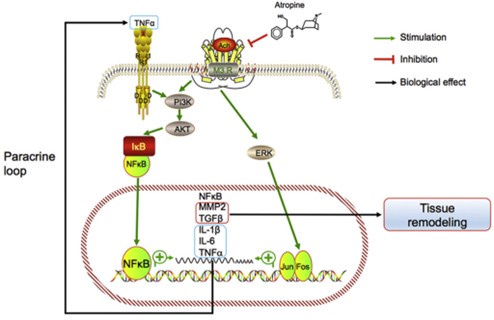
Model of the association between inflammation and myopia progression. Activated mAChR3 (M3R) activates phosphoinositide 3-kinase (PI3K)–AKT and mitogen-associated protein kinase (MAPK) signaling pathways, in turn activating NF-κB and AP1 (i.e., the Jun.-Fos heterodimer) and stimulating the expression of the target genes NF-κB, MMP2, TGFβ, IL- 1β and -6, and TNF-α. MMP2 and TGF-β promote tissue remodeling and TNF-α may act in a paracrine feedback loop in the retina or sclera to activate NF-κB during myopia progression.
To address the limitations raised, we will prioritize the following in future studies: Cell-type-specific knockout models to identify key cellular contributors. Mechanistic investigations to establish causal relationships between signaling pathways and myopia progression. We sincerely appreciate your rigorous review, which has significantly improved the scientific accuracy and clarity of our manuscript. We believe the revised version better reflects both the novelty and limitations of our findings. We kindly request your recognition of the study’s contributions while acknowledging its current constraints.
Reviewer #3 (Public review):
Chen et al have identified a new candidate gene for high myopia, ZC3H11A, and using a knock-out mouse model, have attempted to validate it as a myopia gene and explain a potential mechanism. They identified 4 heterozygous missense variants in highly myopic teenagers. These variants are in conserved regions of the protein, and predicted to be damaging, but the only evidence the authors provide that these specific variants affect protein function is a supplement figure showing decreased levels of IκBα after transfection with overexpression plasmids (not specified what type of cells were transfected). This does not prove that these mutations cause loss of function, in fact it implies they have a gain-of-function mechanism. They then created a knock-out mouse. Heterozygotes show myopia at all ages examined but increased axial length only at very early ages. Unfortunately, the authors do not address this point or examine corneal structure in these animals. They show that the mice have decreased B-wave amplitude on electroretinogram (a sign of retinal dysfunction associated with bipolar cells), and decreased expression of a bipolar cell marker, PKCα. On electron microscopy, there are morphologic differences in the outer nuclear layer (where bipolar, amacrine, and horizontal cell bodies reside). Transcriptome analysis identified over 700 differentially expressed genes. The authors chose to focus on the PI3K-AKT and NF-κB signaling pathways and show changes in expression of genes and proteins in those pathways, including PI3K, AKT, IκBα, NF-κB, TGF-β1, MMP-2 and IL-6, although there is very high variability between animals. They propose that myopia may develop in these animals either as a result of visual abnormality (decreased bipolar cell function in the retina) or by alteration of NF-κB signaling. These data provide an interesting new candidate variant for development of high myopia, and provide additional data that MMP2 and IL6 have a role in myopia development. For this revision, none of my previous suggestions have been addressed.
Reviewer #3 (Recommendations for the authors):
None of these suggestions were addressed in the revision:
Major issues:
(1) Figure 2: refraction is more myopic but axial length is not longer - why is this not discussed and explored? The text claims the axial length is longer, but that is not supported by the figure. If this is a measurement issue, that needs to be discussed in the text.
We sincerely appreciate your valuable comments regarding the relationship between refractive status and axial length in our study. In response to your concerns, we have conducted an in-depth analysis and would like to address the issues as follows:
Our data demonstrate significant differences in refractive error between heterozygous (Het) and wild-type (WT) mice during the 4-10 weeks. Notably, at 4 and 6 weeks of age, Het mice did exhibit longer axial lengths and greater vitreous chamber depth compared to WT mice, although these differences did not reach statistical significance at other time points while still showing an increasing trend. Additional measurements of corneal curvature revealed no significant differences between groups. Considering the small size of mouse eyes (where a 1D refractive change corresponds to only 5-6μm axial length change) and the theoretical resolution limit of 6μm for the SD-OCT device used in this study, these technical factors may account for the marginal statistical significance of the observed small changes in vitreous chamber depth and axial length measurements. Furthermore, existing studies have shown that axial length measurements from frozen sections tend to be longer than those obtained from in vivo measurements in age-matched mice. These considerations provide plausible explanations for the apparent discrepancy between refractive changes and axial length parameters. Following your suggestion, we have added a dedicated discussion section addressing these axial length measurement issues in the revised manuscript. We fully understand your concerns regarding data consistency, and your comments have prompted us to conduct more comprehensive and thorough analysis of our results. We believe the revised manuscript now more accurately reflects our findings while providing important technical references for future studies.
(2) Slipped into the methods is a statement that mice with small eyes or ocular lesions were excluded. How many mice were excluded? Are the authors ignoring another phenotype of these mice?
We appreciate your attention to the exclusion criteria and their implications. Below we provide a detailed clarification: A total of 7 mice (4 Het-KO and 3 WT) with small eyes or ocular lesions were excluded from the observation cohort. These anomalies were consistent with the baseline incidence of spontaneous malformations observed in historical colony data of wild-type C57BL/6J mice (approximately 11%), and were not attributed to the Zc3h11a heterozygous knockout. We have added the above content in the methods section. Your insightful comment has significantly strengthened our reporting rigor. We hope this clarification alleviates your concerns regarding potential selection bias or overlooked phenotypes.
Minor/Word choice issues:
All the figure legends need to be improved so that each figure can be interpreted without having to refer to the text.
Thank you for your valuable comments. We have made modifications to the legend of each graphic, as detailed in the main text.
Abstract: line 24: use refraction, not "vision"
Thank you for your valuable comments. The “Vision” has been changed to “refraction”.
Line 28: re-word "density of bipolar cell-labeled proteins" Do the authors mean density of bipolar cells? Or certain proteins were less abundant in bipolar cells?
Thank you for your rigorous review of this terminology. We acknowledge the need to clarify the precise meaning of the phrase "density of bipolar cell-labeled proteins." In the original text, this term specifically refers to the expression abundance of the bipolar cell-specific marker protein PKCα, which was identified using immunofluorescence labeling techniques. Specifically: We utilized PKCα (a bipolar cell marker) to label bipolar cell populations. The "density" was quantified by measuring the fluorescence signal intensity per unit area in confocal microscopy images, rather than direct cell counting. This metric reflects changes in the expression of the specific marker protein (PKCα) within bipolar cells, which indirectly correlates with alterations in bipolar cell populations. To address ambiguity, we have revised the terminology throughout the manuscript to "bipolar cell-labelled protein PKCα immunofluorescence abundance".
Additionally, since fluorescence intensity quantification is inherently semi-quantitative, we have included Western blot results for PKCα in the revised manuscript (Figure 3I, J) to validate the expression changes observed via immunofluorescence. We sincerely appreciate your feedback, which has significantly improved the precision of our manuscript.
Line 45: axial length, not ocular axis
Thank you for your valuable comments. The “ocular axis” has been changed to “axial length”.
Lines73-75: confusing
Thank you for your valuable comments. The relevant content has been modified to “Multiple zinc finger protein genes (e.g., ZNF644, ZC3H11B, ZFP161, ZENK) are associated with myopia or HM. Of these, ZC3H11B (a human homolog of ZC3H11A) and five GWAS loci (Schippert et al., 2007; Shi et al., 2011; Szczerkowska et al., 2019; Tang et al., 2020; Wang et al., 2004) correlate with AL elongation or HM severity. Proteomic studies further suggest ZC3H11A involvement in the TREX complex, implicating RNA export mechanisms in myopia pathogenesis”
Line 138: what is dark 3.0 and dark 10.0
Thank you for your valuable comments. The relevant content has been modified to “Upon dark adaptation, b-wave amplitudes in seven-week-old Het-KO mice were significantly lower at dark 3.0 (0.48 log cd·s/m²) and dark 10.0 (0.98 log cd·s/m²) compared to WT mice.” A detailed description has been added to the main text methods.
Line 171-175: the GO terms of "biological processes" and "molecular functions" are so broad as to be meaningless.
Thank you for your valuable comments. The relevant content has been modified to “GO enrichment analysis revealed significant enrichment of differentially expressed genes in the following functions: Zinc ion transmembrane transport (GO:0071577) within metal ion homeostasis, associated with retinal photoreceptor maintenance (Ugarte and Osborne, 2001), RNA biosynthesis and metabolism (GO:0006366) in transcriptional regulation, potentially influencing ocular development, negative regulation of NF-κB signaling (GO:0043124) in inflammatory modulation, a pathway involved in scleral remodelling (Xiao et al., 2025), calcium ion binding (GO:0005509), critical for phototransduction (Krizaj and Copenhagen, 2002), zinc ion transmembrane transporter activity (GO:0005385), participating in retinal zinc homeostasis (Figure 5C and D).”
Line 257-259: which results indicated loss of Zc3h11a inhibited translocation of IκBα from nucleus to cytoplasm? Results of this study, or the previously referenced study?
We sincerely appreciate your critical inquiry regarding the mechanistic relationship between Zc3h11a deficiency and IκBα translocation. We are grateful for this opportunity to clarify this important point. The findings regarding Zc3h11a-mediated regulation of IκBα mRNA nuclear export and its impact on NF-κB signaling originate from the study by Darweesh et al. The key experimental evidence demonstrates that: The depletion of Zc3h11a leads to nuclear retention of IκBα mRNA, resulting in failure to maintain normal levels of cytoplasmic IκBα mRNA and protein. This defect in IκBα mRNA export disrupts the essential inhibitory feedback loop on NF-κB activity, causing hyperactivation of this pathway. This manifests as upregulation of numerous innate immune-related mRNAs, including IL-6 and a large group of interferon-stimulated genes.While our study references this mechanism to explain the observed NF-κB dysregulation in Zc3h11a Het-KO mice, the specific nuclear export mechanism was indeed elucidated by Darweesh et al. The reference has been inserted into the corresponding position in the main text. Importantly, our research extends these previous molecular insights into the phenotypic context of myopia.
We sincerely regret any ambiguity in the original text and deeply appreciate your rigorous approach in ensuring proper attribution of these fundamental findings. Your comment has significantly improved the clarity and accuracy of our manuscript.
Figure 6 shows decrease of both mRNA and protein expression, but nothing about translocation.
Thank you for your valuable comments. The research results of Darweesh et al. showed that Zc3h11a protein plays a role in regulation of NF-κB signal transduction. Depletion of Zc3h11a resulted in enhanced NF-κB mediated signaling, with upregulation of numerous innate immune related mRNAs, including IL-6 and a large group of interferon-stimulated genes. IL-6 upregulation in the absence of the Zc3h11a protein correlated with an increased NF-κB transcription factor binding to the IL-6 promoter and decreased IL-6 mRNA decay. The enhanced NF-κB signaling pathway in Zc3h11a deficient cells correlated with a defect in IκBα inhibitory mRNA and protein accumulation. Upon Zc3h11a depletion The IκBα mRNA was retained in the cell nucleus resulting in failure to maintain normal levels of the cytoplasmic IκBα mRNA and protein that is essential for its inhibitory feedback loop on NF-κB activity. These findings demonstrate that ZC3H11A can regulate the NF-κB pathway by controlling the translocation of IκBα mRNA, a mechanism that was indeed elucidated by Darweesh et al. We sincerely apologize for any lack of clarity in our original description and have now inserted the appropriate reference in the relevant section of the main text.
We deeply appreciate your valuable comments in identifying this ambiguity in our manuscript, which have significantly improved the accuracy and clarity of our work.
Line 283: what do you mean "may confer embryonic lethality"? Were they embryonic lethal or not?
We sincerely appreciate your critical request for clarification. Our experimental data from 15 pregnancies of Zc3h11a Het-KO mice intercrosses (n = 15 litters) conclusively confirmed the absence of homozygous knockout (Homo-KO) pups at birth. These findings align with the embryonic lethality of Zc3h11a homozygous deletion as reported by Younis et al. We fully acknowledge the ambiguity in our original phrasing and have revised the text to:“Second, Zc3h11a homozygous KO (Homo-KO) mice were not obtained in our study because homozygous deletion of exons confer embryonic lethality.”Your vigilance in ensuring terminological precision has greatly strengthened the rigor of our manuscript. We hope this clarification fully resolves your concerns.
Line 338: What is meant that Het-KO mice were constructed at 4 weeks of age? Do these mice not have a germline mutation?
Thank you for your valuable comments. We have revised the following content: “The germline heterozygous Zc3h11a knockout (Het-KO) mice were generated by CRISPR/Cas9-mediated gene editing at the embryonic stage on a C57BL/6J background, provided by GemPharmatech Co., Ltd (Nanjing, China). Phenotypic analyses were initiated when the mice reached four weeks of age.”
Line 346-347: how many mice were excluded due to having small eyes or ocular lesions? The methods section should state how refraction and ocular biometrics were measured.
Thank you for your valuable comments. We have added or revised the following content: “To exclude potential confounding effects of spontaneous ocular developmental abnormalities, a total of 7 mice (4 Het-KO and 3 WT) with small eyes or ocular lesions were excluded from the observation cohort. These anomalies were consistent with the baseline incidence of spontaneous malformations observed in historical colony data of wild-type C57BL/6J mice (approximately 11%), and were not attributed to the Zc3h11a heterozygous knockout.
The methods for measuring refraction and ocular biometrics are as follows and have been added to the original method. Refractive measurements were performed by a researcher blinded to the genotypes. Briefly, in a darkroom, mice were gently restrained by tail-holding on a platform facing an eccentric infrared retinoscope (EIR) (Schaeffel et al., 2004; Zhou et al., 2008a). The operator swiftly aligned the mouse position to obtain crisp Purkinje images centered on the pupil using detection software (Schaeffel et al., 2004), enabling axial measurements of refractive state and pupil size. Three repeated measurements per eye were averaged for analysis. The anterior chamber (AC) depth, lens thickness, vitreous chamber (VC) depth, and axial length (AL) of the eye were measured by real-time optical coherence tomography (a custom built OCT) (Zhou et al., 2008b). In simple terms, after anesthesia, each mouse was placed in a cylindrical holder on a positioning stage in front of the optical scanning probe. A video monitoring system was used to observe the eyes during the process. Additionally, by detecting the specular reflection on the corneal apex and the posterior lens apex in the two dimensional OCT image, the optical axis of the mouse eye was aligned with the axis of the probe. Eye dimensions were determined by moving the focal plane with a stepper motor and recording the distance between the interfaces of the eyes. Then, using the designed MATLAB software and appropriate refractive indices, the recorded optical path length was converted into geometric path length. Each eye was scanned three times, and the average value was taken.”
Line 428: what age retinas
Thank you for your meticulous attention to the experimental design details. Regarding the age of retinal samples, we have clarified the following in the revised manuscript:" Retinas were harvested from four-week-old mice for RNA sequencing." This revision enhances the transparency and reproducibility of our methodology. We deeply appreciate your rigorous review.
Figure 3 D-F: these images are too small to adequately assess, please show at higher magnification. Are there fewer bipolar cells, or just decreased expression of PKC? From these images, expression of ZC3H11A does not appear decreased, but the retina appears thinner. Is that true, or are these poorly matched sections?
Thank you for your professional insights regarding image quality and data interpretation. Your rigorous review has significantly enhanced the scientific rigor of our study. We hereby address your concerns point by point: The images in Figures 3D-F were acquired using a Zeiss LSM880 confocal microscope with a 10x eyepiece and 20x objective lens, a standard magnification for retinal section imaging that balances cellular resolution with full-thickness structural preservation. We quantified PKCα immunofluorescence intensity (a bipolar cell-specific marker) to assess changes in bipolar cell populations, rather than direct cell counting. This metric reflects PKCα expression abundance as a proxy for bipolar cell alterations (Figure 3H). To clarify terminology, we have revised the text to "bipolar cell-labelled protein PKCα immunofluorescence abundance" and detailed the methodology in the revised Methods section. Recognizing the semi-quantitative nature of fluorescence intensity analysis, we supplemented these data with Western blot results confirming reduced PKCα protein levels (Figure 3I). Zc3h11a expression was validated both by immunofluorescence intensity (Figure 3G) and Western blot (Figures 6F, H) quantification, confirming reduced expression in Zc3h11a Het-KO retinas. The apparent "retinal thinning" observed in histology sections stems from technical artifacts during tissue processing (fixation, dehydration, sectioning), not biological differences. HE staining, which better preserves sample morphology, showed no structural or thickness differences between Zc3h11a Het-KO mice and wild-type mice (Supplementary Figure 2).
Your expert feedback has driven us to establish a more robust validation framework. We believe the revised data now more accurately reflect the biological reality and sincerely hope these improvements meet your approval.
Figure 3G-J: Relative fluorescence intensity of immunohistochemistry is not a valid measure of protein expression.
We sincerely appreciate your thorough review and valuable comments regarding the immunofluorescence quantification method in Figures 3G-J. In response to your concern that "relative fluorescence intensity is not an effective quantitative measure of protein expression," we have implemented the following improvements to our analysis and validation: To ensure result reliability, all immunofluorescence experiments followed strict protocols: experimental and control samples were fixed, stained, and imaged in the same batch to eliminate inter-batch variability. Imaging was performed using a Zeiss LSM 880 confocal microscope with identical parameters, and the relative fluorescence intensity of specific signals per unit area was measured and statistically analyzed using ZEN software. We fully acknowledge the semi-quantitative nature of relative fluorescence intensity measurements. Therefore, we validated key differentially expressed proteins using Western blot analysis: The Western blot results for Zc3h11a (Figures 6F, H) were completely consistent with the relative fluorescence intensity trends (Figure 3G). Additionally, the newly included Western blot data for PKCα (Figure 3 I) further confirmed the reliability of our relative fluorescence intensity quantification. Your expert advice has significantly enhanced the rigor of our study. Should any additional data or clarification be required, we would be pleased to provide further support.
Figure 4: what are the arrows pointing at? This should be in the Figure legend. What is MB? Why are there no scale bars? What is difference between E and F, not clear from legend.
We sincerely appreciate your thorough review of Figure 4 and your valuable suggestions. In response to your concerns, we have carefully examined and improved the relevant content with the following modifications and clarifications: We sincerely apologize for not clearly indicating the arrow annotations in the original figure legend. In the revised version, we have provided detailed explanations for the arrow indicators: black arrows indicate perinuclear space dilation, blue arrows indicate cytoplasmic edema, and red arrows indicate disorganized and loosely arranged membrane discs. The updated legend has been clearly marked below Figure 4 in the main text. MB represents membrane discs, which are critical subcellular structures in the outer segments of retinal photoreceptor cells (rods and cones). They are responsible for light signal capture and transduction (containing visual pigments such as rhodopsin). The structural integrity of MB is essential for normal visual function. The scale bars in the original figures were located in the lower right corner of each subpanel, with specific parameters as follows: Figures 4A and B: magnification ×1000, scale bar 10 μm; Figures 4C and D: magnification ×700, scale bar 20 μm; Figures 4E and G: magnification ×2000, scale bar 5 μm; Figures 4F and H: magnification ×7000, scale bar 2 μm. Both Figures 4E and 4F show electron microscopy images of membrane discs (MB) in wild-type mouse photoreceptor cells. The only difference lies in the magnification: Figure 4E (×2000) demonstrates the overall arrangement pattern of membrane discs, while Figure 4F (×7000) focuses on ultrastructural details of the membrane discs (such as structural integrity). We have thoroughly checked the consistency between the figures and text, and have supplemented detailed legend descriptions in the main text. Once again, we sincerely appreciate your rigorous review, which has significantly enhanced the scientific rigor and readability of our study. Should you have any further suggestions, we would be happy to incorporate them.
Figure 5A: Why such a large y-axis? Figure legend does not match figure
We sincerely appreciate your careful review of Figure 5A and your valuable suggestions regarding the figure details. In response to your concerns, we have thoroughly examined and improved the relevant content as follows: The Y-axis of the volcano plot represents -log₁₀(p-value), where the magnitude of the values reflects statistical significance. Our RNA-seq data underwent rigorous multiple testing correction, and the adjusted p-values for some genes were extremely small, resulting in large values after -log₁₀ transformation. We have re-examined the data distribution and confirmed that the expanded Y-axis range is solely due to a small number of highly significant genes (as shown in the figure, the majority of genes remain clustered in the lower half of the Y-axis). This result accurately reflects the true data characteristics.
We sincerely apologize for the inadvertent error in the original labeling of "Up/Down" in the figure legend. This has now been corrected, and we strictly adhere to the following threshold criteria: Significantly upregulated (Up): adjusted p-value < 0.05 and log₂(FC) ≥ 1. Significantly downregulated (Down): adjusted p-value < 0.05 and log₂(FC) ≤ -1. To ensure the reliability of our conclusions, we have rechecked the raw data, statistical analysis, and visualization process. We confirmed that all significant genes strictly meet the above threshold criteria and that the visualization accurately reflects the true results. The revised figure has been updated in the manuscript as Figure 5A. We deeply appreciate your valuable feedback, which has helped us correct the errors in the figure and improve its accuracy and readability.
Figure 6F: Based on the western blot, only Zc3h11a appears different.
Thank you for your careful evaluation of the Western blot data in Figure 6F. We fully understand your concerns regarding the visual differences in PI3K and p-AKT/AKT bands and appreciate the opportunity to clarify the quantitative methodology and biological significance of these findings. Below we provide a detailed explanation of the experimental design and data analysis.
First, the data for each group were derived from retinal samples of three independent mice, with all experiments performed in parallel to control for technical variability. Image analysis was conducted using ImageJ software with standardized settings for grayscale quantification. Zc3h11a and PI3K levels were normalized to GAPDH as an internal reference, while p-AKT levels were calculated as a ratio to total AKT. The results showed that Zc3h11a protein levels were significantly reduced (p < 0.01, Figures 6F and H), consistent with the expected effects of heterozygous knockout, with good agreement between visual and statistical results. For PI3K and p-AKT/AKT, the bands appeared visually similar due to: The nonlinear nature of Western blot chemiluminescence signals in the saturation range, which compresses subtle quantitative differences in the images; the fact that p-AKT represents only 5-15% of the total AKT pool, making small proportional changes difficult to discern visually. However, it is important to note that both PI3K and p-AKT/AKT showed statistically significant differences between groups (p < 0.001 and p < 0.01, respectively; Figures 6G and I). Furthermore, signal transduction pathways exhibit cascade amplification effects - in the PI3K-AKT pathway, even small changes in upstream proteins can produce significant downstream effects (e.g., NF-κB activation) through kinase cascades (Figure 6J). Additionally, our RNA-Seq results revealed activation of the PI3K-AKT signaling pathway in Zc3h11a Het-KO mice (Figure 5D), and the qRT-PCR results were consistent with the western blot results (Figure 6A-C). Your expert comments have prompted us to present these data differences with greater biological rigor. Although the visual differences are subtle, based on statistical significance, pathway characteristics, and RNA sequencing, and qRT-PCR data, we believe these changes have biological relevance. We sincerely appreciate your commitment to data rigor and respectfully request your recognition of both the experimental results and the scientific logic of this study.
Figure 8: What is the role of ZC3H11A in this figure? Are the authors proposing that ZC3H11A regulates the translation of IκBα? They have not shown any evidence of that.
Thank you for your insightful exploration of the role of ZC3H11A in Figure 8. We appreciate your critical review and hope to elucidate the mechanistic framework behind our findings. In Figure 8, Zc3h11a is depicted as a regulator of IκBα mRNA nucleocytoplasmic transport, a mechanism originally elucidated by Darweesh et al. Their studies demonstrated that Zc3h11a binds to IκBα mRNA and promotes its nuclear export. Loss of Zc3h11a results in nuclear retention of IκBα mRNA, leading to reduced cytoplasmic IκBα protein levels and subsequent hyperactivation of the NF-κB pathway. While the specific nuclear export mechanism has been elucidated by Darweesh et al., our study demonstrates that Zc3h11a haploinsufficiency results in decreased IκBα mRNA and protein levels in the retina (Figure 7), linking Zc3h11a haploinsufficiency to NF-κB pathway dysregulation in myopia and highlighting that these molecular insights can be extended to a new pathological context (myopia). Your critical comments have enhanced the clarity of our mechanistic concepts and we hope that these descriptions will demonstrate the importance of ZC3H11A as a new candidate gene for myopia.
Author response:
The following is the authors’ response to the previous reviews.
Public Reviews:
Reviewer #1 (Public review):
Summary:
Shen et al. conducted three experiments to study the cortical tracking of the natural rhythms involved in biological motion (BM), and whether these involve audiovisual integration (AVI). They presented participants with visual (dot) motion and/or the sound of a walking person. They found that EEG activity tracks the step rhythm, as well as the gait (2-step cycle) rhythm. The gait rhythm specifically is tracked superadditively (power for A+V condition is higher than the sum of the A-only and V-only condition, Experiments 1a/b), which is independent of the specific step frequency (Experiment 1b). Furthermore, audiovisual integration during tracking of gait was specific to BM, as it was absent (that is, the audiovisual congruency effect) when the walking dot motion was vertically inverted (Experiment 2). Finally, the study shows that an individual's autistic traits are negatively correlated with the BM-AVI congruency effect.
Strengths:
The three experiments are well designed and the various conditions are well controlled. The rationale of the study is clear, and the manuscript is pleasant to read. The analysis choices are easy to follow, and mostly appropriate.
Weaknesses:
There is a concern of double-dipping in one of the tests (Experiment 2, Figure 3: interaction of Upright/Inverted X Congruent/Incongruent). I raised this concern on the original submission, and it has not been resolved properly. The follow-up statistical test (after channel selection using the interaction contrast permutation test) still is geared towards that same contrast, even though the latter is now being tested differently. (Perhaps not explicitly testing the interaction, but in essence still testing the same.) A very simple solution would be to remove the post-hoc statistical tests and simply acknowledge that you're comparing simple means, while the statistical assessment was already taken care of using the permutation test. (In other words: the data appear compelling because of the cluster test, but NOT because of the subsequent t-tests.)
We are sorry that we did not explain this issue clearly before, which might have caused some misunderstanding. When performing the cluster-based permutation test, we only tested whether the audiovisual congruency effect (congruent vs. incongruent) between the upright and inverted conditions was significantly different [i.e., (UprCon – UprInc) vs. (InvCon – InvInc)], without conducting extra statistical analyses on whether the congruency effect was significant in each orientation condition. Such an analysis yielded a cluster with a significant interaction between audiovisual integration and BM orientation for the cortical tracking effect at 1Hz (but not at 2Hz). However, this does not provide valid information about whether the audiovisual congruency effect at this cluster is significant in each orientation condition, given that a significant interaction effect may result from various patterns of data across conditions: such as significant congruency effects in both orientation conditions (Author response image 1a), a significant congruency effect in the upright condition and a non-significant effect in the inverted condition (Author response image 1b), or even non-significant yet opposite effects in the two conditions (Author response image 1c). Here, our results conform to the second pattern, indicating that cortical tracking of the high-order gait cycles involves a domain-specific process exclusively engaged in the AVI of BM. In a similar vein, the non-significant interaction found at 2Hz does not necessarily indicate that the congruency effect is non-significant in each orientation condition (Author response image 1f&e). Indeed, the congruency effect was significant in both the upright and inverted conditions at 2Hz in our study despite the non-significant interaction, suggesting that neural tracking of the lower-order step cycles is associated with a domain-general AVI process mostly driven by temporal correspondence in physical stimuli.
Therefore, we need to perform subsequent t-tests to examine the significance of the simple effects in the two orientation conditions, which do not duplicate the clusterbased permutation test (for interaction only) and cause no double-dipping. Results from interaction and simple effects, put together, provide solid evidence that the cortical tracking of higher-order and lower-order rhythms involves BM-specific and domaingeneral audiovisual processing, respectively.
To avoid ambiguity, we have removed the sentence “We calculated the audiovisual congruency effect for the upright and the inverted conditions” (line 194, which referred to the calculation of the indices rather than any statistical tests) from the manuscript. We have also clarified the meanings of the findings based on the interaction and simple effects together at the two temporal scales, respectively (Lines 205-207; Lines 213-215).
Author response image 1.
Examples of different patterns of data yielding a significant or nonsignificant interaction effect.
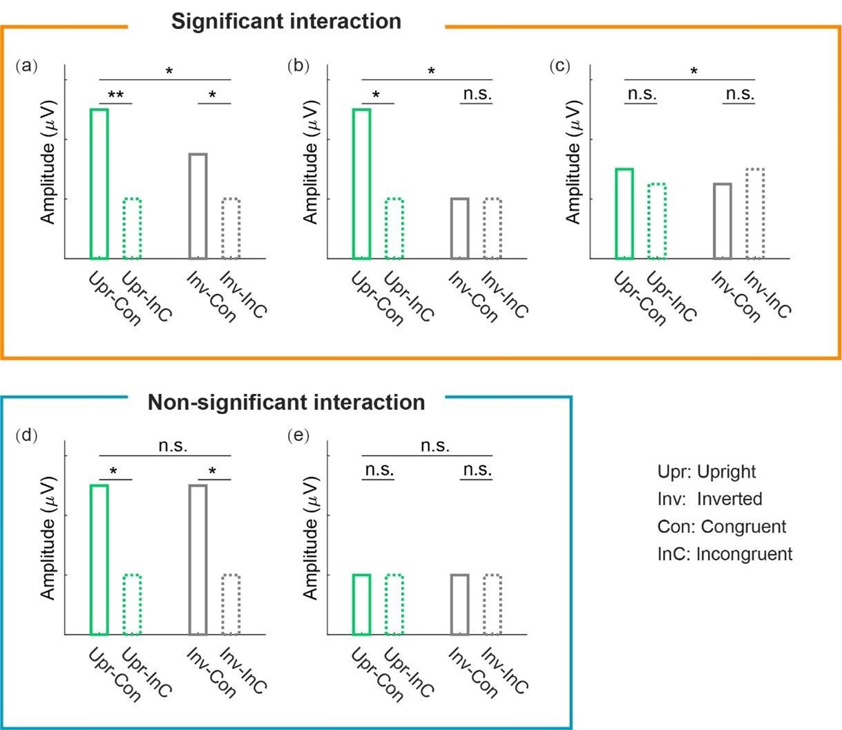
Reviewer #2 (Public review):
Summary:
The authors evaluate spectral changes in electroencephalography (EEG) data as a function of the congruency of audio and visual information associated with biological motion (BM) or non-biological motion. The results show supra-additive power gains in the neural response to gait dynamics, with trials in which audio and visual information was presented simultaneously producing higher average amplitude than the combined average power for auditory and visual conditions alone. Further analyses suggest that such supra-additivity is specific to BM and emerges from temporoparietal areas. The authors also find that the BM-specific supra-additivity is negatively correlated with autism traits.
Strengths:
The manuscript is well-written, with a concise and clear writing style. The visual presentation is largely clear. The study involves multiple experiments with different participant groups. Each experiment involves specific considered changes to the experimental paradigm that both replicate the previous experiment's finding yet extend it in a relevant manner.
Weaknesses:
In the revised version of the paper, the manuscript better relays the results and anticipates analyses, and this version adequately resolves some concerns I had about analysis details. Still, it is my view that the findings of the study are basic neural correlate results that do not provide insights into neural mechanisms or the causal relevance of neural effects towards behavior and cognition. The presence of an inversion effect suggests that the supra-additivity is related to cognition, but that leaves open whether any detected neural pattern is actually consequential for multi-sensory integration (i.e., correlation is not causation). In other words, the fact that frequency-specific neural responses to the [audio & visual] condition are stronger than those to [audio] and [visual] combined does not mean this has implications for behavioral performance. While the correlation to autism traits could suggest some relation to behavior and is interesting in its own right, this correlation is a highly indirect way of assessing behavioral relevance. It would be helpful to test the relevance of supra-additive cortical tracking on a behavioral task directly related to the processing of biological motion to justify the claim that inputs are being integrated in the service of behavior. Under either framework, cortical tracking or entrainment, the causal relevance of neural findings toward cognition is lacking.
Overall, I believe this study finds neural correlates of biological motion, and it is possible that such neural correlates relate to behaviorally relevant neural mechanisms, but based on the current task and associated analyses this has not been shown.
Thank you for providing these thoughtful comments regarding the theoretical implications of our neural findings. Previous behavioral evidence highlights the specificity of the audiovisual integration (AVI) of biological motion (BM) and reveals the impairment of such ability in individuals with autism spectrum disorder. However, the neural implementation underlying the AVI of BM, its specificity, and its association with autistic traits remain largely unknown. The current study aimed to address these issues.
It is noteworthy that the operation of multisensory integration does not always depend on specific tasks, as our brains tend to integrate signals from different sensory modalities even when there is no explicit task. Hence, many studies have investigated multisensory integration at the neural level without examining its correlation with behavioral performance. For example, the widely known super-additivity mode for multisensory integration proposed by Perrault and colleagues was based on single-cell recording findings without behavioral tasks (Perrault et al., 2003, 2005). As we mentioned in the manuscript, the super-additive and sub-additive modes indicate non-linear interaction processing, either with potentiated neural activation to facilitate the perception or detection of near-threshold signals (super-additive) or a deactivation mechanism to minimize the processing of redundant information cross-modally (subadditive) (Laurienti et al., 2005; Metzger et al., 2020; Stanford et al., 2005; Wright et al., 2003). Meanwhile, the additive integration mode represents a linear combination between two modalities. Distinguishing among these integration modes helps elucidate the neural mechanism underlying AVI in specific contexts, even though sometimes, the neural-level AVI effects do not directly correspond to a significant behavioral-level AVI effect (Ahmed et al., 2023; Metzger et al., 2020). In the current study, we unveiled the dissociation of multisensory integration modes between neural responses at two temporal scales (Exps. 1a & 1b), which may involve the cooperation of a domain-specific and a domain-general AVI processes (Exp. 2). While these findings were not expected to be captured by a single behavioral index, they revealed the multifaceted mechanism whereby hierarchical cortical activity supports audiovisual BM integration. They also advance our understanding of the emerging view that multi-timescale neural dynamics coordinate multisensory integration (Senkowski & Engel, 2024), especially from the perspective of natural stimuli processing.
Meanwhile, our finding that the cortical tracking of higher-order rhythmic structure in audiovisual BM specifically correlated with individual autistic traits extends previous behavioral evidence that ASD children exhibited reduced orienting to audiovisual synchrony in BM (Falck-Ytter et al., 2018), offering new evidence that individual differences in audiovisual BM processing are present at the neural level and associated with autistic traits. This finding opens the possibility of utilizing the cortical tracking of BM as a potential neural maker to assist the diagnosis of autism spectrum disorder (see more details in our Discussion Lines 334-346).
However, despite the main objective of the current study focusing on the neural processing of BM, we agree with the reviewer that it would be helpful to test the relevance of supra-additive cortical tracking on a behavioral task directly related to BM perception, for further justifying that inputs are being integrated in the service of behavior. In the current study, we adopted a color-change detection task entirely unrelated to audiovisual correspondence but only for maintaining participants’ attention. The advantage of this design is that it allows us to investigate whether and how the human brain integrates audiovisual BM information under task-irrelevant settings, as people in daily life can integrate such information even without a relevant task. However, this advantage is accompanied by a limitation: the task does not facilitate the direct examination of the correlation between neural responses and behavioral performance, since the task performance was generally high (mean accuracy >98% in all experiments). Future research could investigate this issue by introducing behavioral tasks more relevant to BM perception (e.g., Shen et al., 2023). They could also apply advanced neuromodulation techniques to elucidate the causal relevance of the cortical tracking effect to behavior (e.g., Ko sem et al., 2018, 2020).
We have discussed the abovementioned points as a separate paragraph in the revised manuscript (Lines 322-333). In addition, since the scope of the current study does not involve a causal correlation with behavioral performance, we have removed or modified the descriptions related to "functional relevance" in the manuscript (Abstract; Introduction, lines 101-103; Results, lines 239; Discussion, line 336; Supplementary Information, line 794、803). Moreover, we have strengthened the descriptions of the theoretical implications of the current findings in the abstract.
We hope these changes adequately address your concern.
References
Ahmed, F., Nidiffer, A. R., O’Sullivan, A. E., Zuk, N. J., & Lalor, E. C. (2023). The integration of continuous audio and visual speech in a cocktail-party environment depends on attention. Neuroimage, 274, 120143. https://doi.org/10.1016/j.neuroimage.2023.120143
Falck-Ytter, T., Nystro m, P., Gredeba ck, G., Gliga, T., Bo lte, S., & the EASE team. (2018). Reduced orienting to audiovisual synchrony in infancy predicts autism diagnosis at 3 years of age. Journal of Child Psychology and Psychiatry, 59(8), 872–880. https://doi.org/10.1111/jcpp.12863
Ko sem, A., Bosker, H., Jensen, O., Hagoort, P., & Riecke, L. (2020). Biasing the Perception of Spoken Words with Transcranial Alternating Current Stimulation. Journal of Cognitive Neuroscience, 32, 1–10. https://doi.org/10.1162/jocn_a_01579
Ko sem, A., Bosker, H. R., Takashima, A., Meyer, A., Jensen, O., & Hagoort, P. (2018). Neural Entrainment Determines the Words We Hear. Current Biology, 28(18), 2867-2875.e3. https://doi.org/10.1016/j.cub.2018.07.023
Laurienti, P. J., Perrault, T. J., Stanford, T. R., Wallace, M. T., & Stein, B. E. (2005). On the use of superadditivity as a metric for characterizing multisensory integration in functional neuroimaging studies. Experimental Brain Research, 166(3), 289–297. https://doi.org/10.1007/s00221-005-2370-2
Metzger, B. A., Magnotti, J. F., Wang, Z., Nesbitt, E., Karas, P. J., Yoshor, D., & Beauchamp, M. S. (2020). Responses to Visual Speech in Human Posterior Superior Temporal Gyrus Examined with iEEG Deconvolution. The Journal of Neuroscience: The Official Journal of the Society for Neuroscience, 40(36), 6938–6948. https://doi.org/10.1523/JNEUROSCI.0279-20.2020
Perrault, T. J., Vaughan, J. W., Stein, B. E., & Wallace, M. T. (2003). Neuron-Specific Response Characteristics Predict the Magnitude of Multisensory Integration. Journal of Neurophysiology, 90(6), 4022–4026. https://doi.org/10.1152/jn.00494.2003
Perrault, T. J., Vaughan, J. W., Stein, B. E., & Wallace, M. T. (2005). Superior Colliculus Neurons Use Distinct Operational Modes in the Integration of Multisensory Stimuli. Journal of Neurophysiology, 93(5), 2575–2586. https://doi.org/10.1152/jn.00926.2004
Senkowski, D., & Engel, A. K. (2024). Multi-timescale neural dynamics for multisensory integration. Nature Reviews Neuroscience, 25(9), 625–642. https://doi.org/10.1038/s41583-024-00845-7
Shen, L., Lu, X., Wang, Y., & Jiang, Y. (2023). Audiovisual correspondence facilitates the visual search for biological motion. Psychonomic Bulletin & Review, 30(6), 2272–2281. https://doi.org/10.3758/s13423-023-02308-z
Stanford, T. R., Quessy, S., & Stein, B. E. (2005). Evaluating the Operations Underlying Multisensory Integration in the Cat Superior Colliculus. Journal of Neuroscience, 25(28), 6499–6508. https://doi.org/10.1523/JNEUROSCI.5095-04.2005
Wright, T. M., Pelphrey, K. A., Allison, T., McKeown, M. J., & McCarthy, G. (2003). Polysensory Interactions along Lateral Temporal Regions Evoked by Audiovisual Speech. Cerebral Cortex, 13(10), 1034–1043. https://doi.org/10.1093/cercor/13.10.1034
Author Response
The following is the authors’ response to the original reviews.
Reviewer #1 (Public Review):
This is an interesting and somewhat unusual paper supporting the idea that creatine is a neurotransmitter in the central nervous system of vertebrates. The idea is not entirely new, and the authors carefully weigh the evidence, both past and newly acquired, to make their case. The strength of the paper lies in the importance of the potential discovery - as the authors point out, creatine ticks more boxes on criteria of neurotransmitters than some of the ones listed in textbooks - and the list of known transmitters (currently 16) certainly is textbook material. A further strength of the manuscript is the careful consideration of a list of criteria for transmitters and newly acquired evidence for four of these criteria: 1. evidence that creatine is stored in synaptic vesicles, 2. mutants for creatine synthesis and a vesicular transporter show reduced storage and release of creatine, 3. functional measurement that creatine release has an excitatory or inhibitory (here inhibitory) effect in vivo, and 4. ATP-dependence. The key weakness of the paper is that there is no single clear 'smoking gun', like a postsynaptic creatine receptor, that would really demonstrate the function as a transmitter. Instead, the evidence is of a cumulative nature, and not all bits of evidence are equally strong. On balance, I found the path to discovery and the evidence assembled in this manuscript to establish a clear possibility, positive evidence, and to provide a foundation for further work in this direction.
it is notable that, historically, no neurotransmitter has ever been established in a single paper. While creatine will not be an exception, data presented in this paper are more than any previous paper in demonstrating the possibility of a new neurotransmitter. However, we added an entire paragraph in the Discussion part about differences between Cr and classic neurotransmitters such as Glu, beginning with the absence of a molecularly defined receptor at this point and the Ca2+ independent component of Cr release induced by extracellular K+.
We appreciate the reviewer for noting that evidence obtained by us now support that creatine satisfies all 4 criteria of transmitters.
We respectively disagree the point about a smoking gun: any of these four is a smoking gun, while the satisfication of all 4 is quite strong, more than a smoking gun.
We find it disagreeable that a receptor “would really demonstrate the function of a transmitter”. Textbook criteria for a transmitter usually require postsynaptic responses, not a molecularly defined receptor. A molecularly defined receptor for many of the known transmitters required many years of work, while they were accepted as transmitters before their receptors were finally molecularly defined. As long as there is a postsynaptic response, there is of course a receptor, though its molecular properties should be further studied. For examples, responses to choline were discovered in 1900 (Hunt, Am J Physiol 3, xviii-xix, 1900), those to acetylcholine in 1906 (Hunt and Taveau, Br Med J 2:1788-1789, 1906), those to supradrenal glands before 1894 (Oliver and Schäfer, J Physiol 18:230-276 1895). Henry Dale was awarded a Nobel prize in 1936 partly for his work on acetylcholine. Receptors for acetylcholine and noradrenaline were not molecularly defined until the 1970s and 1980s. Before then, they were only known by mediating responses to natural transmitters and synthesized chemicals.
There were two previous reports that creatine could be taken into brain slices (Almeida et al., 2006) or synaptosomes (Peral, Vázquez-Carretero and Ilundain, 2010). These were used by the reviewer to argue that the idea of creatine as a neurotransmitter “is not entirely new”. However, no one has followed up these studies for 10 years, thus they would not be considered as good smoking guns. While we have reproduced the synaptosome uptake result (together with our new finding that this uptake was dependent on SLC6A8), it should be noted that uptake of molecules into synaptosomes is not absolutely required for a neurotransmitter because degradation of a transmitter is equally valid. Furthermore, molecules required synaptically but not as a transmitter can also be transported into the synaptic terminal.
Our detection of Cr in the synaptic vesicles provides much stronger evidence supporting its importance. If a smoking gun is important, the detection of creatine in the SVs is the best smoking gun, whose discovery in fact was the reason leading us to study its release, postsynaptic responses as well as repeating the uptake experiment with genetic mutants.
Reviewer #2 (Public Review):
Summary:
Bian et al studied creatine (Cr) in the context of central nervous system (CNS) function. They detected Cr in synaptic vesicles purified from mouse brains with anti-Synaptophysin using capillary electrophoresis-mass spectrometry. Cr levels in the synaptic vesicle fraction were reduced in mice lacking the Cr synthetase AGAT, or the Cr transporter SLC6A8. They provide evidence for Cr release within several minutes after treating brain slices with KCl. This KCl-induced Cr release was partially calcium-dependent and was attenuated in slices obtained from AGAT and SLC6A8 mutant mice. Cr application also decreased the excitability of cortical pyramidal cells in one third of the cells tested. Finally, they provide evidence for SLC6A8-dependent Cr uptake into synaptosomes, and ATP-dependent Cr loading into synaptic vesicles. Based on these data, the authors propose that Cr may act as a neurotransmitter in the CNS.
Strengths:
1) A major strength of the paper is the broad spectrum of tools used to investigate Cr.
2) The study provides strong evidence that Cr is present in/loaded into synaptic vesicles.
Weaknesses:
(in sequential order)
1) Are Cr levels indeed reduced in Agat-/-? The decrease in Cr IgG in Agat-/- (and Agat+/-) is similar to the corresponding decrease in Syp (Fig. 3B). What is the explanation for this? Is the decrease in Cr in Agat-/- significant when considering the drop in IgG? The data should be normalized to the respective IgG control.
We measured the Cr concentration in the whole brain lysates using Creatine Assay Kit (Sigma, MAK079). Cr levels in the brain were reduced in Agat-/- mice. The Cr concentration in AGAT-/- mice was reduced to about 1/10 of AGAT+/+ and AGAT+/- mice (Author response image 1).
Author response image 1.
Cr concentration in brain from AGAT+/+, AGAT+/- and AGAT-/- mice (n=5 male mice for each group). , p<0.05, **, p<0.001, one-way ANOVA with Tukey’s correction.
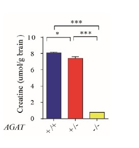
As pointed by the reviewer, the decrease in Cr IgG in Agat-/- seems similar to the corresponding decrease in Syp (Fig. 3B in the paper). Cr pulled down by IgG was 0.46 ± 0.04, 0.37 ± 0.06 and 0.17 ±0.03 pmol/μg anti-syp antibody for Agat+/+, Agat+/-, and Agat-/- mice respectively. There was a trend of reduction Cr IgG in Agat-/-, however, there were no statistically significant differences between Agat-/- and Agat+/+, or between Agat-/- and Agat+/-, as determined by one-way ANOVA (Fig. 3B in the paper). Due to the fact that Agat-/- reduced Cr concentration in the brain, we speculate that the apparent drop in Cr pulled down by IgG may have partially resulted from the overall reduction of Cr content in the brain.
The absolute content of Cr pulled down by Syp in Agat-/- mice was reduced to 21.6% of Agat+/+ mice and 23.6% of Agat+/- mice (Fig. 3B in the paper). As suggested by the reviewer, we normalized the Cr pulled down by Syp to the respective IgG control (Author response image 2). The normalized Cr content in AGAT-/- mice has a tendency to decrease, but not statistically significant, as compared to Agat+/+ and Agat+/- mice (n=10 for each group, one-way ANOVA).
Author response image 2.
Normalized Cr content in brain from AGAT+/+, AGAT+/- and AGAT-/- mice (n=10 for each group). Cr pulled down by anti-Syp antibody was normalized to that of IgG.
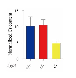
2) The data supporting that depolarization-induced Cr release is SLC6A8 dependent is not convincing because the relative increase in KCl-induced Cr release is similar between SLC6A8-/Y and SLC6A8+/Y (Fig. 5D). The data should be also normalized to the respective controls.
As suggested by the reviewer, we normalized the Cr release during KCl stimulation to the baseline (Author response image 3). The ratio of Cr release evoked by high KCl stimulation to the baseline was similar in WT and Slc6a8 knockouts. This suggests that Cr is not released through SLC6A8 transporter.
Author response image 3.
Normalized Cr release from slices from Slc6a8+/Y and Slc6a8-/Y mice (n=7 slices for each group). Cr released evoked by high KCl stimulation was normalized to baseline.
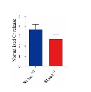
However, without Slc6a8, KCl-induced release of Cr was significantly reduced (Figure 5D in the paper). This is because Slc6a8 is a transporter to Cr uptake into synaptic terminals (Figure 5D and 8C in the paper). Therefore, Cr content in SVs (Figure 2C in the paper) indirectly reduced Cr release.
3) The majority (almost 3/4) of depolarization-induced Cr release is Ca2+ independent (Fig. 5G). Furthermore, KCl-induced, Ca2+-independent release persists in SLC6A8-/Y (Fig. 5G). What is the model for Ca2+-independent Cr release? Why is there Ca2+-independent Cr release from SLC6A8 KO neurons? How does this relate to the prominent decrease in Ca2+-dependent Cr release in SLC6A8-/Y (Fig. 5G)? They show a prominent decrease in Cr control levels in SLC6A8-/Y in Fig. 5D. Were the data shown in Fig. 5D obtained in the presence or absence of Ca2+? Could the decrease in Ca2+-dependent Cr release in SLC6A8-/Y (Fig. 5G) be due to decreased Cr baseline levels in the presence of Ca2+ (Fig. 5D)?
These are interesting questions that, at this point, could only be answered by references to literature. For example, one possibility was that Ca2+-independent Cr release might occurs in glia, since as pointed by the reviewer in Point 6, high GAMT levels were reported for astrocytes and oligodendrites (Schmidt et al. 2004; Rosko et al. 2023). As reported, other neuromodulators such as taurine can be released from astrocytes (Philibert, Rogers, and Dutton 1989) or slices (Saransaari and Oja 2006) in Ca2+ independent manner. In addition, in the absence of potassium stimulation, Ca2+ depletion lead to increased release of taurine in cultured astrocytes (Takuma et al. 1996) or in striatum in vivo (Molchanova, Oja, and Saransaari 2005). Similarly, in SLC6A8 KO slices, Ca2+ depletion (Figure 5G) also increased creatine baseline levels as compared to that in normal ACSF (Figure 5D). Another possibility was that Ca2+-independent Cr release might occurs in neurons lacking SLC6a8 expression.
As mentioned in the paper, data shown in Figure 5D was obtained in the presence Ca2+. Reduction of Ca2+-dependent Cr release evoked by potassium in SLC6A8-/Y (Figure 5G) may be due to decreased Cr baseline levels in the presence of Ca2+ and reduced Cr in synaptic vesicles (Figure 5D).
4) Cr levels are strongly reduced in Agat-/- (Figure 6B). However, KCl-induced Cr release persists after loss of AGAT (Figure 6B). These data do not support that Cr release is Agat dependent.
Although KCl-induced Cr release persisted in AGAT-/- mutants, it was dropped to 11.6% of WT mice (Figure 6B). AGAT is not directly involved in the release, but required for providing sufficient Cr.
5) The authors show that Cr application decreases excitability in ~1/3 of the tested neurons (Figure 7). How were responders and non-responders defined? What justifies this classification? The data for all Cr-treated cells should be pooled. Are there indeed two distributions (responders/non-responders)? Running statistics on pre-selected groups (Figure 7H-J) is meaningless. Given that the effects could be seen 2-8 minutes after Cr application - at what time points were the data shown in Figure 7E-J collected? Is the Cr group shown in Figure 7F significantly different from the control group/wash?
The responders were defined by three criteria: (1) When Cr was applied, the rheobase was increased as compared to both control and wash conditions. (2) The number of total evoked spikes was decreased during Cr application than both control and wash. (3) The number of total evoked spikes was decreased at least by 10% than control or wash.
For all the individual responders, when Cr was applied, the rheobase was increased (Figure 7E and 7F). While in individual non-responders, the rheobase was either identical to both control and wash (n=19/35), identical to either control or wash (n=11/35), between control and wash (n=2/35) or smaller than both control and wash (n=3/35) following Cr application. Thus, the responders and non-responders were separatable. When the rheobase data were pulled together, many points were overlapped, so we did not pull the data here.
As suggested, we pulled the data of the ratio of spike changes in response to 100 μM Cr application for all neurons together (Author response image 4). Evoked spikes of non-responders were typically (34/35) changed in the range of -10% to 10%.
Author response image 4.
Relative changes of total evoked spikes in response to 100 μM Cr. Responders are represented by red dots and non-responders by black dots. Dashed black line indicates 10%. Relative change = (Cr-(Control +wash)/2)/((Control +wash)/2)*100%.
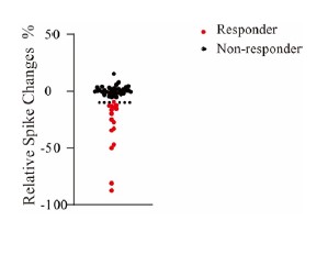
In Figure 7E-J, we collected data at time points when the maximal response was reached. The Cr group shown in Figure 7F was indeed significantly different from the control group/wash (p<0.05, paired t test, for data points collected under 75-500 pA current injection).
6) Indirect effects: The phenotypes could be partially caused by indirect effects of perturbing the Cr/PCr/CK system, which is known to play essential roles in ATP regeneration, Ca2+ homeostasis, neurotransmission, intracellular signaling systems, axonal and dendritic transport... Similarly, high GAMT levels were reported for astrocytes (e.g., Schmidt et al. 2004; doi: 10.1093/hmg/ddh112), and changes in astrocytic Cr may underlie the phenotypes. Cr has been also reported to be an osmolyte: a hyperosmotic shock of astrocytes induced an increase in Cr uptake, suggesting that Cr can work as a compensatory osmolyte (Alfieri et al. 2006; doi: 10.1113/jphysiol.2006.115006). Potential indirect effects are also consistent with a trend towards decreased KCl-induced GABA (and Glutamate) release in SLC6A8-/Y (Figure 5C). These indirect effects may in part explain the phenotypes seen after perturbing Agat, SLC6A8, and should be thoroughly discussed.
We discussed the possibility of creatine/phosphocreatine as non-transmitters in discussion part. We added the possibility of astrocytic Cr in discussion part. KCl-induced GABA (and Glutamate) release in SLC6A8-/Y (Figure 5C) was not significant.
7) As stated by the authors, there is some evidence that Cr may act as a co-transmitter for GABAA receptors (although only at high concentrations). Would a GABAA blocker decrease the fraction of cells with decreased excitability after Cr exposure?
We performed another experiment in CA1 pyramidal neurons in hippocampus showing that Cr at 100 μM did not change GABAergic neurotransmission (n=8, Author response image 5). Inhibitory postsynaptic currents (IPSCs) recorded in the presence of glutamate receptor blockers (10 μM APV and 10 μM CNQX) were not changed by 100 μM creatine in hippocampal CA1 pyramidal neurons (Bgroup data of IPSC frequency (B) and amplitude (C) averaged in 1 min duration). These did not support Cr activation of GABAA receptors.
Author response image 5.
IPSCs recorded in in hippocampal CA1 pyramidal neurons. (A) representative raw traces before (Control), during (Creatine) and after (Wash) the application of 100 μM creatine. (B&C) group data of IPSC frequency (B) and amplitude (C) averaged in 1 min duration.
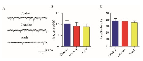
8) The statement "Our results have also satisfied the criteria of Purves et al. 67,68, because the presence of postsynaptic receptors can be inferred by postsynaptic responses." (l.568) is not supported by the data and should be removed.
We have deleted this sentence, though what could mediate postsynaptic responses other than receptors?
Reviewer #3 (Public Review):
SUMMARY:
The manuscript by Bian et al. promotes the idea that creatine is a new neurotransmitter. The authors conduct an impressive combination of mass spectrometry (Fig. 1), genetics (Figs. 2, 3, 6), biochemistry (Figs. 2, 3, 8), immunostaining (Fig. 4), electrophysiology (Figs. 5, 6, 7), and EM (Fig. 8) in order to offer support for the hypothesis that creatine is a CNS neurotransmitter.
We thank the reviewer for the summary.
STRENGTHS:
There are many strengths to this study.
• The combinatorial approach is a strength. There is no shortage of data in this study.
• The careful consideration of specific criteria that creatine would need to meet in order to be considered a neurotransmitter is a strength.
• The comparison studies that the authors have done in parallel with classical neurotransmitters are helpful.
• Demonstration that creatine has inhibitory effects is another strength.
• The new genetic mutations for Slc6a8 and AGAT are strengths and potentially incredibly helpful for downstream work.
WEAKNESSES:
• Some data are indirect. Even though Slc6a8 and AGAT are helpful sentinels for the presence of creatine, they are not creatine themselves. Therefore, the conclusions that are drawn should be circumspect.
SLC6A8 and AGAT mutants are not essential for Cr’s role as a neurotransmitter.
• Regarding Slc6a8, it seems to work only as a reuptake transporter - not as a transporter into SVs. Therefore, we do not know what the transporter is.
Indeed, SLC6A8 is only a transporter on the cytoplasmic membrane, not a transporter on synaptic vesicles. We have shown biochemistry here, and we have unpublished data that showed other SLCs on SVs, which did not include SLC6A8.
• Puzzlingly, Slc6a8 and AGAT are in different cells, setting up the complicated model that creatine is created in one cell type and then processed as a neurotransmitter in another.
• No candidate receptor for creatine has been identified postsynaptically.
• Because no candidate receptor has been identified, is it possible that creatine is exerting its effects indirectly through other inhibitory receptors (e.g., GABAergic Rs)?
As shown in our response to Question 7 of Reviewer 2, Cr did not exert its effects through inhibitory GABAA receptors.
• More broadly, what are the other possibilities for roles of creatine that would explain these observations other than it being a neurotransmitter? Could it simply be a modifier that exists in the SVs (lots of molecules exist in SVs)?
We discussed the possibility of a non-transmitter role for creatine/phosphocreatine in discussion part.
• The biochemical studies are helpful in terms of comparing relevant molecules (e.g., Figs. 8 and S1), but the images of the westerns are all so fuzzy that there are questions about processing and the accuracy of the quantification.
Multiple members (>4) have carried out SV purifications repeatedly over the last decade in our group, we are highly confident of SV purifications presented in Figs. 8 and S1.
There are several criteria that define a neurotransmitter. The authors nicely delineated many criteria in their discussion, but it is worth it for readers to do the same with their own understanding of the data.
By this reviewer's understanding (and the Purves' textbook definition) a neurotransmitter: 1) must be present within the presynaptic neuron and stored in vesicles; 2) must be released by depolarization of the presynaptic terminal; 3) must require Ca2+ influx upon depolarization prior to release; 4) must bind specific receptors present on the postsynaptic cell; 5) exogenous transmitter can mimic presynaptic release; 6) there exists a mechanism of removal of the neurotransmitter from the synaptic cleft.
6 criteria seem to be only required by the reviewer. As discussed in our Discussion part, Purves’ textbook did not list 6 criteria but only three criteria, “the substance must be present within the presynaptic neuron; the substance must be released in response to presynaptic depolarization, and the release must be Ca2+ dependent; specific receptors for the substance be present on the postsynaptic cell” (Purves et al., 2001, 2016).
Kandel et al. (2013, 2021) listed 4 criteria for a neurotransmitter: “it is synthesized in the presynaptic neuron; it is present within vesicles and is released in amounts sufficient to exert a defined action on the postsynaptic neuron or effector organ; when administered exogenously in reasonable concentrations it mimics the action of the endogenous transmitter; a specific mechanism usually exists for removing the substance from the synaptic cleft”.
While we agree that any neuroscientist can have his/her own criteria, it is more reasonable to accept the textbooks that have been widely read for decades.
For a paper to claim that the work has identified a new neurotransmitter, several of these criteria would be met - and the paper would acknowledge in the discussion which ones have not been met. For this particular paper, this reviewer finds that condition 1 is clearly met.
Conditions 2 and 3 seem to be met by electrophysiology, but there are caveats here. High KCl stimulation is a blunt instrument that will depolarize absolutely everything in the prep all at once and could result in any number of non-specific biological reactions as a result of K+ rushing into all neurons in the prep. Moreover, the results in 0 Ca2+ are puzzling. For creatine (and for the other neurotransmitters), why is there such a massive uptick in release, even when the extracellular saline is devoid of calcium?
To avoid the disadvantage of high KCl stimulation, we performed optogenetic experiments recently, with encouraging preliminary data. We do not know the source of Ca2+-independent release of Cr and neurotransmitters, though astrocytes are a possibility.
Condition 4 is not discussed in detail at all. In the discussion, the authors elide the criterion of receptors specified by Purves by inferring that the existence of postsynaptic responses implies the existence of receptors. True, but does it specifically imply the existence of creatinergic receptors? This reviewer does not think that is necessarily the case. The authors should be appropriately circumspect and consider other modes of inhibition that are induced by activation or potentiation of other receptors (e.g., GABAergic or glycinergic).
Our results did not support Cr stimulation of inhibitory GABAA receptors (see our answer to Point 7 in of Reviewer 2).
Condition 5 may be met, because the authors applied exogenous creatine and observed inhibition (Fig. 7). However, this is tough to know without understanding the effects of endogenous release of creatine. if they were to test if the absence of creatine caused excess excitation (at putative creatinergic synapses), then that would be supportive of the same.
After the submission of our manuscript, we found a recent paper showing that slc6a8 knockout led to increased excitation in pyramidal neurons in the prefrontal cortex (PFC), with increased firing frequency (Ghirardini et al., 2023). Because we have shown that slc6a8 knockout would cause decrease of Cr in SVs (Figure 2 in our paper), this result provide the evidence described as Condition 5 of this reviewer: that decrease of Cr in SVs led to excess excitation.
For condition 6, the authors made a great effort with Slc6a8. This is a very tough criterion to understand for many synapses and neurotransmitters.
In terms of fundamental neuroscience, the story would be impactful if proven correct. There are certainly more neurotransmitters out there than currently identified.
The impact as framed by the authors in the abstract and introduction for intellectual disability is uncertain (forming a "new basis for ID pathogenesis") and it seems quite speculative beyond the data in this paper.
We deleted this sentence.
Reviewer #1 (Recommendations For The Authors):
To strengthen the manuscript, I suggest the following considerations:
1) The key missing evidence to my mind is a receptor - but this is clearly outside the scope of this paper. Yet, I am surprised that in the list of criteria for neurotransmitters in general there is no mention of a receptor. Furthermore, many receptors have been identified through receptor agonists or antagonists, like neurotoxins or drugs. The authors do not talk about putative receptors except for a sentence in the discussion where they speculate on a GPCR. There are numerous GPCR agonists and antagonists, which may be a long-shot, or something even a bit more designed based on knowledge about creatine? I do not think the publication of this manuscript should have been made dependent on finding an agonist or antagonist of this specific unknown receptor (if it exists), but it would be good to have at least some leads on this from the authors what has been tried or what could be done? How about a manipulation of G-protein-coupled signal transduction to support the idea that there IS such a GPCR? There may be a real opportunity here to test existing compounds in wild type, the slc6a8 and agat mutants.
We will keep trying, but accept the reality that Rome was not built in a single day and that no transmitter was proven by one single paper.
A key new puzzle piece of evidence is the identification of creatine in synaptic vesicles. The experiment relies heavily on the purity of the SV fraction using the anti-synaptophysin antibody. I am quite sure that these preparations contain many other compartments - and of course a big mix of synaptic (and other) vesicles. Would it be possible to purify with an anti slc6a8 antibody?
Sl6a8 is expressed in on the plasma membrane of neurons7-9, instead of synaptic vesicles. Consistent with this, we could not detect obvious Slc6a8-HA signal in our starting material (Lane S in Author response image 6) that was used for SV purification. We have tried to purify SVs by HA antibody in Slc6a8 mice and SV markers could not be detected.
Author response image 6.
Lack of Slc6a8-HA in our starting material. In Slc6a8-HA knock-in mice, the HA signal was present in whole brain homogenate (H), but not obvious in supernatants (S) following 35000 × centrifugation. In contrast, SV marker Syp was present in supernatants.
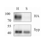
The K stimulation protocol in slices is relatively crude, as all neurons in the slice get simultaneously overactivated - and some of the effects on Ca-dependent release are not very strong (e.g. the 35 neurons that were not responsive to creatine at all). A primary neuronal culture of neurons that respond to creatine would strengthen this section.
To avoid the disadvantage of K stimulation, we also performed optogenetic experiments recently and obtained encouraging preliminary results.
Reviewer #2 (Recommendations For The Authors):
1) The different sections of the manuscript are not separated by headers.
2) The beginning of the results section either does not reference the underlying literature or refers to unpublished data.
We have kept a bit background in the beginning of the Results section.
3) The text contains many opinions and historical information that are not required (e.g., "It has never been easy to discover a new neurotransmitter, especially one in the central nervous system (CNS). We have been searching for new neurotransmitters for 12 years."; l. 17).
This is a field that has been dormant for decades and such background introductions are helpful for at least some readers.
4) Almeida et al. (2008; doi: 10.1002/syn.20280) provided evidence for electrical activity-, and Ca2+-dependent Cr release from rat brain slices. This paper should be introduced in the introduction.
Those were stand-alone papers which have not been reproduced or paid attention to. Our introduction part did not mention them because our research did not begin with those papers. We had no idea that those papers existed when we began. We started with SV purification and only read those papers afterwards. Thus, they were not necessary background to our paper but can be discussed after we discovered Cr in SVs.
5) Fig. 7: A Y-scale for the stimulation protocol is missing.
Revised.
Reviewer #3 (Recommendations For The Authors):
The main suggestion by this reviewer (beyond the details in the public review) is to consider the full spectrum of biology that is consistent with these results. By my reading, creatine could be a neurotransmitter, but other possibilities also exist, and the authors need to highlight those too.
We have discussed non-transmitter role in the discussion.
References
Ghirardini, E., G. Sagona, A. Marquez-Galera, F. Calugi, C. M. Navarron, F. Cacciante, S. Chen, F. Di Vetta, L. Dada, R. Mazziotti, L. Lupori, E. Putignano, P. Baldi, J. P. Lopez-Atalaya, T. Pizzorusso, and L. Baroncelli. 2023. Cell-specific vulnerability to metabolic failure: the crucial role of parvalbumin expressing neurons in creatine transporter deficiency. Acta Neuropathol Commun, 11: 34. doi: 10.1186/s40478-023-01533-w.
Lowe, M. T., Faull, R. L., Christie, D. L. & Waldvogel, H. J. Distribution of the creatine transporter throughout the human brain reveals a spectrum of creatine transporter immunoreactivity. J Comp Neurol 523, 699-725 (2015). https://doi.org:10.1002/cne.23667
Mak, C. S. et al. Immunohistochemical localisation of the creatine transporter in the rat brain. Neuroscience 163, 571-585 (2009). https://doi.org:10.1016/j.neuroscience.2009.06.065.
Molchanova, S. M., Oja, S. S. & Saransaari, P. Mechanisms of enhanced taurine release under Ca2+ depletion. Neurochem Int 47, 343-349 (2005). https://doi.org:10.1016/j.neuint.2005.04.027
Philibert, R. A., Rogers, K. L. & Dutton, G. R. K+-evoked taurine efflux from cerebellar astrocytes: on the roles of Ca2+ and Na+. Neurochem Res 14, 43-48 (1989). https://doi.org:10.1007/BF00969756
Rosko, L. M. et al. Cerebral Creatine Deficiency Affects the Timing of Oligodendrocyte Myelination. J Neurosci 43, 1143-1153 (2023). https://doi.org:10.1523/JNEUROSCI.2120-21.2022
Saransaari, P. & Oja, S. S. Characteristics of taurine release in slices from adult and developing mouse brain stem. Amino Acids 31, 35-43 (2006). https://doi.org:10.1007/s00726-006-0290-5
Schmidt, A. et al. Severely altered guanidino compound levels, disturbed body weight homeostasis and impaired fertility in a mouse model of guanidinoacetate N-methyltransferase (GAMT) deficiency. Hum Mol Genet 13, 905-921 (2004). https://doi.org:10.1093/hmg/ddh112
Speer, O. et al. Creatine transporters: a reappraisal. Mol Cell Biochem 256-257, 407-424 (2004). https://doi.org:10.1023/b:mcbi.0000009886.98508.e7
Takuma, K. et al. Ca2+ depletion facilitates taurine release in cultured rat astrocytes. Jpn J Pharmacol 72, 75-78 (1996). https://doi.org:10.1254/jjp.72.75
Author Response
The following is the authors’ response to the previous reviews.
eLife assessment
This valuable paper examines gene expression differences between male and female individuals over the course of flower development in the dioecious angiosperm Trichosantes pilosa. The authors show that male-biased genes evolve faster than female-biased and unbiased genes. This is frequently observed in animals, but this is the first report of such a pattern in plants. In spite of the limited sample size, the evidence is mostly solid and the methods appropriate for a non-model organism. The resources produced will be used by researchers working in the Cucurbitaceae, and the results obtained advance our understanding of the mechanisms of plant sexual reproduction and its evolutionary implications: as such they will broadly appeal to evolutionary biologists and plant biologists.
Public Reviews:
Reviewer #1 (Public Review):
The evolution of dioecy in angiosperms has significant implications for plant reproductive efficiency, adaptation, evolutionary potential, and resilience to environmental changes. Dioecy allows for the specialization and division of labor between male and female plants, where each sex can focus on specific aspects of reproduction and allocate resources accordingly. This division of labor creates an opportunity for sexual selection to act and can drive the evolution of sexual dimorphism.
In the present study, the authors investigate sex-biased gene expression patterns in juvenile and mature dioecious flowers to gain insights into the molecular basis of sexual dimorphism. They find that a large proportion of the plant transcriptome is differentially regulated between males and females with the number of sex-biased genes in floral buds being approximately 15 times higher than in mature flowers. The functional analysis of sex-biased genes reveals that chemical defense pathways against herbivores are up-regulated in the female buds along with genes involved in the acquisition of resources such as carbon for fruit and seed production, whereas male buds are enriched in genes related to signaling, inflorescence development and senescence of male flowers. Furthermore, the authors implement sophisticated maximum likelihood methods to understand the forces driving the evolution of sex-biased genes. They highlight the influence of positive and relaxed purifying selection on the evolution of male-biased genes, which show significantly higher rates of non-synonymous to synonymous substitutions than female or unbiased genes. This is the first report (to my knowledge) highlighting the occurrence of this pattern in plants. Overall, this study provides important insights into the genetic basis of sexual dimorphism and the evolution of reproductive genes in Cucurbitaceae.
Reviewer #2 (Public Review):
Summary:
This study uses transcriptome sequence from a dioecious plant to compare evolutionary rates between genes with male- and female-biased expression and distinguish between relaxed selection and positive selection as causes for more rapid evolution. These questions have been explored in animals and algae, but few studies have investigated this in dioecious angiosperms, and none have so far identified faster rates of evolution in male-biased genes (though see Hough et al. 2014 https://doi.org/10.1073/pnas.1319227111).
Strengths:
The methods are appropriate to the questions asked. Both the sample size and the depth of sequencing are sufficient, and the methods used to estimate evolutionary rates and the strength of selection are appropriate. The data presented are consistent with faster evolution of genes with male-biased expression, due to both positive and relaxed selection.
This is a useful contribution to understanding the effect of sex-biased expression in genetic evolution in plants. It demonstrates the range of variation in evolutionary rates and selective mechanisms, and provides further context to connect these patterns to potential explanatory factors in plant diversity such as the age of sex chromosomes and the developmental trajectories of male and female flowers.
Weaknesses:
The presence of sex chromosomes is a potential confounding factor, since there are different evolutionary expectations for X-linked, Y-linked, and autosomal genes. Attempting to distinguish transcripts on the sex chromosomes from autosomal transcripts could provide additional insight into the relative contributions of positive and relaxed selection.
Reviewer #3 (Public Review):
The potential for sexual selection and the extent of sexual dimorphism in gene expression have been studied in great detail in animals, but hardly examined in plants so far. In this context, the study by Zhao, Zhou et al. al represents a welcome addition to the literature.
Relative to the previous studies in Angiosperms, the dataset is interesting in that it focuses on reproductive rather than somatic tissues (which makes sense to investigate sexual selection), and includes more than a single developmental stage (buds + mature flowers).<br /> Some aspects of the presentation have been improved in this new version of the manuscript.
Specifically:
the link between sex-biased and tissue-biased genes is now slightly clearer,
the limitation related to the de novo assembled transcriptome is now formally acknowledged,
the interpretation of functional categories of the genes identified is more precise,
the legends of supplementary figures have been improved - a large number of typos have been fixed.
in response to this first round of reviews. As I detail below, many of the relevant and constructive suggestions by the previous reviewers were not taken into account in this revision.
For instance:
- Reviewer 2 made precise suggestions for trying to take into account the potential confounding factor of sex-chromosomes. This suggestion was not followed.
For the question of reviewer 2:
The presence of sex chromosomes is a potential confounding factor, since there are different evolutionary expectations for X-linked, Y-linked, and autosomal genes. Attempting to distinguish transcripts on the sex chromosomes from autosomal transcripts could provide additional insight into the relative contributions of positive and relaxed selection.
Empirically, the analyses could be expanded by an attempt to distinguish between genes on the autosomes and the sex chromosomes. Genotypic patterns can be used to provisionally assign transcripts to XY or XX-like behavior when all males are heterozygous and all females are homozygous (fixed X-Y SNPs) and when all females are heterozygous and males are homozygous (lost or silenced Y genes). Comparing such genes to autosomal genes with sex-biased expression would sharpen the results because there are different expectations for the efficacy of selection on sex chromosomes. See this paper (Hough et al. 2014; https://www.pnas.org/doi/abs/10.1073/pnas.1319227111), which should be cited and does in fact identify faster substitution rates in Y-linked genes.
Authors’ response: We have cited Hough et al. (2014) and Sandler et al. (2018) in the revised manuscript. We agree that the presence of sex chromosomes is potentially a confounding factor. By adopting methods in Hough et al. (2014) and Sandler et al. (2018), we tried to distinguish transcripts on sex chromosomes from autosomal chromosomes. For a total of 2,378 unbiased genes, we found that 36 genes were putatively sex chromosomal genes, 20 of which were exclusively heterozygous and homozygous for males and females, respectively; while the other 16 genes showing an opposite genotyping patterns between males and females. For 343 male-biased genes, only three ones exhibit a pattern of potentially sex-linked. For the 1,145 female-biased genes, we identified 19 genes which might located on the sex chromosomes. Among the 19 genes, five genes were exclusively heterozygous for males and exclusively homozygous for females, while reversed genotyping patterns presented in the other 14 genes. So, sex-linked genes may contribute relatively little to rapid evolution of male-biased genes. An alternative explanation is that the results could be unreliable due to small sample sizes. Thus, we did not describe them in the Results section. We will investigate the issue when whole genome sequences and population datasets become available in the near future.
- Reviewer 1 & 3 indicated that results were mentioned in the discussion section without having been described before. This was not fixed in this new version.
For the question of reviewer 1:
2) Paragraph (407-416) describes the analysis of duplicated genes under relaxed selection but there is no mention of this in the results.
Authors’ response: Following this suggestion, in the Results section, we have added a sentence, “We also found that most of them were members of different gene families generated by gene duplication (Table S13)” on line 310-311 in the revised manuscript (Rapid_evolution_of_malebiased_genes_Trichosanthes_pilosa_Tracked_change_2023_11_06.docx).
For the question of reviewer 1:
38- line 417-424. The discussion should not contain new results.
Authors’ response: Thank you for pointing out this. In the Results section, we have added a few sentences as following: “Similarly, given that dN/dS values of sex-biased genes were higher due to codon usage bias, lower dS rates would be expected in sex-biased genes relative to unbiased genes (Ellegren & Parsch, 2007; Parvathy et al., 2022). However, in our results, the median of dS values in male-biased genes were much higher than those in female-biased and unbiased genes in the results of ‘free-ratio’ (Fig. S4A, female-biased versus male-biased genes, P = 6.444e-12 and malebiased versus unbiased genes, P = 4.564e-13) and ‘two-ratio’ branch model (Fig. S4B, femalebiased versus male-biased genes, P = 2.2e-16 and male-biased versus unbiased genes, P = 9.421e08, respectively). ” on line 323-331, and consequently, removed the following sentence, “femalebiased vs male-biased genes, P = 6.444e-12 and male-biased vs unbiased genes, P = 4.564e-13” and “female-biased versus male-biased genes, P = 2.2e-16 and male-biased versus unbiased genes, P = 9.421e-08, respectively” in the Discussion section.
- Reviewer 1 asked for a comparison between the number of de novo assembled unigenes in this transcriptome and the number of genes in other Cucurbitaceae species. I could not see this comparison reported.
Authors’ response: In the first revision, we described only percentages. We have now added the number of genes. We modify this part as follows: “The majority of unigenes were annotated by homologs in species of Cucurbitaceae (61.6%, 36,375), including Momordica charantia (16.3%, 9,625), Cucumis melo (11.9%, 7,027), Cucurbita pepo (11.9%, 7,027), Cucurbita moschata (11.5%, 6,791), Cucurbita maxima (10.1%, 5,964) and other species (38.4%, 22,676) (Fig. S1C).”.
- Reviewer 1 pointed out that permutation tests were more appropriate, but no change was made to the manuscript.
Authors’ response: Thank you for your suggestion. In the first revision, we have indirectly responded to the issues. Wilcoxon rank sum test is more commonly used for all comparisons between sex-biased and unbiased genes in many papers. Additionally, we tested datasets using permutation t-tests, which is consistent with the results of Wilcoxon rank sum test. For example, we found that only in floral buds, there are significant differences in ω values in the results of ‘free-ratio’ (female-biased versus male-biased genes, P = 0.04282 and male-biased versus unbiased genes, P = 0.01114) and ‘two-ratio’ model (female-biased versus male-biased genes, P = 0.01992 and male-biased versus unbiased genes, P = 0.02127, respectively). We also described these results in the Results section accordingly (line 278-284).
- Reviewer 3 pointed out the small sample size (both for the RNA-seq and the phylogenetic analysis), but again this limitation is not acknowledged very clearly.
Authors’ response: Sorry, we acknowledged that our sample size was relatively small. In the revised version, we have added a sentence as follows, “Additionally, our sample size is relatively small, and may provide low power to detect differential expression.” in the Discussion section.
- Reviewer 1 & 3 pointed out that Fig 3 was hard to understand and asked for clarifications that I did not see in the text and the figure in unchanged.
Authors’ response: Thank you for your suggestions. We have revised the manuscript to clarify the meaning of the acronym (F1TGs, F2TGs, M1TGs, M2TGs, F1BGs, F2BGs, M1BGs and M2BGs) and presented the number of genes. We have added two labels, indicating that panels A and B correspond to males and C and D to females in Fig. 3.
- Reviewer 3 suggested to combine all genes with sex-bias expression when evaluating the evolutionary rate, in addition to the analyses already done. This suggestion was not followed.
For the question of reviewer 3:line 196 and following: In these analyses, I could not understand the rationale for keeping buds vs mature flowers as separate analyses throughout. Why not combine both and use the full set of genes showing sex-bias in any tissue? This would increase the power and make the presentation of the results a lot more straightforward.
Authors’ response: Thank you for your suggestions. In the first revision, we tried to respond to the issues. First, we observed strong sexual dimorphism in floral buds, such as racemose versus solitary, early-flowering versus late-flowering. Second, as you pointed out earlier, “the dataset is interesting in that it focuses on reproductive rather than somatic tissues (which makes sense to investigate sexual selection), and includes more than a single developmental stage (buds + mature flowers)”, we totally agree with you on this point. Third, according to your suggestions, we combined all genes with sex-bias expression to evaluate the evolutionary rates. We found significant differences (please see a Figure below) in ω values in the results of ‘free-ratio’ (female-biased versus male-biased genes, P =0.005622 and male-biased versus unbiased genes, P = 0.001961) and ‘two-ratio’ model (female-biased versus male-biased genes, P = 0.008546 and male-biased versus unbiased genes, P = 0.009831, respectively) using Wilcoxon rank sum test. However, the significance is lower than previous results in floral buds due to sex-biased genes of mature flower joined, especially compared to the results of “free-ratio model”. Additionally, we also test all combined genes with sex-bias expression using permutation t-test. Unfortunately, there are no significant differences in ω values expect for male-biased versus unbiased genes in the results of ‘free-ratio’ model (P = 0.03034) and ‘two-ratio’ model (P = 0.0376), respectively. To a certain extent, the combination of all genes with sex-bias expression may cover the signals of rapid evolution of sex-biased genes in floral buds. Therefore, these results are not described in our manuscript. In the near future, we would like to make further investigations through more development stages of flowers and new technologies (e.g. Single-Cell method, See Murat et al., 2023) in each sex to consolidate the conclusion, and it is hoped that we could find more meaningful results.
Author response image 1.
- Reviewer 3 pointed out that hand-picking specific categories of genes was not statistically valid, and in fact not necessary in the present context. This was not changed.
For the question of reviewer3: removing genes on a post-hoc basis seems statistically suspicious to me. I don't think your analysis has enough power to hand-pick specific categories of genes, and it is not clear what this brings here. I suggest simply removing these analyses and paragraphs.
Authors’ response: Thank you for your suggestions. We have changed them accordingly. We removed a part of the following paragraph, “To confirm the contributions of positive selection and relaxed selection to rapid rates of male-biased genes in floral buds, we generated three datasets of OGs by excluding different sets of genes. Specifically, we excluded 18 relaxed selective male-biased genes (5.23%), 98 positively selected male-biased genes (28.57%), and 112 male-biased genes (32.65%) under positive and relaxed selection from 343 OGs (Fig. S4). We observed that after excluding male-biased genes under relaxed purifying selection, the median (0.264) decreased by 0.34% compared to the median (0.265) of all OGs (Fig. S4A-B). However, after excluding positively selected male-biased genes, the median (0.236) was reduced by 11% (Fig. S4A, C) in the results of ‘free-ratio’ branch model. This pattern was consistent with the results of ‘two-ratio’ branch model as well (Fig. S4E-G).” on line 290 to 300.
However, we kept the following paragraph, “We also analyzed female-biased and unbiased genes that underwent positive and relaxed selection in floral buds (Tables S6-S10). We identified 216 (18.86%) positively selected, and 69 (6.03%) relaxed selective female-biased genes from 1,145 OGs, respectively. Similarly, we found 436 (18.33%) positively selected, and 43 (1.81%) unbiased genes under relaxed selection from 2,378 OGs, respectively. Notably, male-biased genes have a higher proportion (10%) of positively selected genes compared to female-biased and unbiased genes. However, relaxed selective male-biased genes have a higher proportion (3.24%) than unbiased genes, but about 0.8% lower than that of female-biased genes.”. In this way, we can compare the proportion of sex-biased genes that have undergone positive selection and release selection among female-biased genes, unbiased genes and male-biased genes in floral buds in the Discussion section.
- Reviewer 1 asked for all data to be public, but I could not find in the manuscript where the link to the data on ResearchGate was provided.
Authors’ response: We have added a link in the Data Availability section.
- Reviewers 1 & 3 pointed out that since only two tissues were compared, the claims on pleiotropy should have been toned down, but no change was made to the text.
Authors’ response: Thank you for your suggestions. We revised “due to low pleiotropic constraints” to “due to low evolutionary constraints” and revised “low pleiotropy” to “low constraints”.
- Reviewer 1 asked for a clarification on which genes are plotted on the heatmap of Fig3C and an explanation of the color scale. No change was made.
Authors’ response: Sorry for the confusion. Actually, Reviewer 1 asked that “Fig. 2C, which genes are plotted on the heatmap and what is the color scale corresponding to?” In the previous revision, we have revised them (See Fig. 2 Sex-biased gene expression for floral buds and flowers at anthesis in males and females of Trichosanthes pilosa). Sex-biased genes (the union of sex-biased genes in F1, M1, F2 and M2) are plotted on the heatmap. The color gradient represents from high to low (from red to green) gene expression.
- Reviewer 1 asked for panel B in Fig S5 and S6 to be removed. They are still there. They asked for abbreviations to be explained in the legend of Fig S8. This was not done. They asked for details about columns headers. Such detailed were not added. They asked for more recent references on line 53-56: this was not done.
Authors’ response: We have removed panel B in Fig. S5 and S6. We explained abbreviations in text and Fig. S8. We added more details about the column headers in Supplementary Table S4, S5, S6, S7, S8, S9 and S10. We also added more recent references on line 53-56.
Recommendations for the authors:
Reviewer #3 (Recommendations For The Authors):
Authors’ response: Thank you for your suggestions. We have revised/fixed these issues following your concerns and suggestions.
Line 46-48 would be clearer as « Sexual dimorphism is the condition where sexes of the same species exhibit different morphological, ecological and physiological traits in gonochoristic animals and dioecious plants, despite male and female individuals sharing the same genome except for sex chromosomes or sex-determining loci »
Authors’ response: Thanks. We have revised it accordingly.
Line 50: replace «in both » by «between the two »
Authors’ response: We have revised it.
Line 51: « genes exclusively » -> « genes expressed exclusively »
Authors’ response: We have revised it.
Line 58: « in many animals » -> « in several animal species »
Authors’ response: We have revised it to “in some animal species”.
Line 58: « to which » -> « of this bias »
Authors’ response: We have revised it.
Line 64: « Most dioecious plants possess homomorphic sex-chromosomes that are roughly similar in size when viewed by light microscopy. » : a reference is missing
Authors’ response: We have added the reference.
Line 67: remove « that »
Authors’ response: We have revised it.
line 96: change to: « only the five above-mentioned studies »
Authors’ response: We have revised it.
Line 97: remove « the »
Authors’ response: We have revised it.
Line 111: « Drosophia » -> Drosophila
Authors’ response: We have revised it.
Line 114: exhibiting -> « exhibited »
Authors’ response: We have revised it.
Line 115: suggest -> « suggesting »
Authors’ response: We have revised it.
Line 117: « studies in plants have rarely reported elevated rates of sex-biased genes » : is it « rarely » or « never » ?
Authors’ response: We have revised to “never”.
Line 143: « It’s » -> « Its »
Authors’ response: We have revised it.
Line 143-146: say whether the male parts (e.g. anthers) are still present in females flowers, and the female parts (pistil+ ovaries) in the male flowers, or whether these respective organs are fully aborted.
Authors’ response: We have added the following sentence, “The male parts (e. g., anthers) of female flowers, and the female parts (e. g., pistil and ovaries) of male flowers are fully aborted” in line 148150 of the Introduction section.
Line 158: this is now clearer, but please specify whether you are talking about 12 floral buds in total, or 12 per individual (i.e. 72 buds in total).
Authors’ response: We have revised it to “Using whole transcriptome shotgun sequencing, we sequenced floral buds and flowers at anthesis from female and male of dioecious T. pilosa. We set up three biological replicates from three female and three male plants, including 12 samples in total (six floral buds and six flowers at anthesis)”.
Line 194-198: These sentences are unclear and hard to link to the figure. Consider changing for « In male plants, the number of tissue-biased genes in flowers at anthesis (M2TGs: n = 2795) was higher than that in floral buds (M1TGs: n = 1755, Fig. 3A and 3B). Figure 3 is also very hard to read. Adding a label on the side to indicate that panels A and B correspond to male-biased genes and C and D to female-biased genes could be useful.
Authors’ response: Thank you for your suggestions. We have revised the text to clarify the meaning of the acronym (F1TGs, F2TGs, M1TGs, M2TGs, F1BGs, F2BGs, M1BGs and M2BGs) and presented the number of genes. We have added two labels, indicating that panels A and B correspond to males and C and D to females in Figure 3.
Line 208: explain the approach: e.g. « We then compared rates of protein evolution among malebiased, female-biased and unbiased genes. To do this, we sequenced floral bud transcriptomes from the closely related T. anguina, as well as two more distant outgroups, T. kirilowii and Luffa cylindrica. T. kirilowii is a dioecious species like T. pilosa, and the other two are monoecious. We identified one-to-one orthologous groups (OGs) for 1,145 female-biased, 343 male-biased, and 2,378 unbiased genes. »
Authors’ response: We have revised this paragraph to the following, “We compared rates of protein evolution among male-biased, female-biased and unbiased genes in four species with phylogenetic relationships (((T. anguina, T. pilosa), T. kirilowii), Luffa cylindrica), including dioecious T. pilosa, dioecious T. kirilowii, monoecious T. anguina in Trichosanthes, together with monoecious Luffa cylindrica. To do this, we sequenced transcriptomes of T. pilosa. We also collected transcriptomes of T. kirilowii, as well as genomes of T. anguina and Luffa cylindrica.”
Line 220: « the same ω value was in all branches » -> « all branches are constrained to have the same ω value ».
Authors’ response: We have revised it.
Line 221: « results of the 'two-ratio' branch model ... »
Authors’ response: We have revised it.
Line 235: add a few words to explain why the effect size is bigger than for buds, but still is not significant: e.g. «possibly because of limited statistical power due to the low number of sex-biased genes in flowers at anthesis »
Authors’ response: We have revised this to “However, there is no statistically significant difference in the distribution of ω values using Wilcoxon rank sum tests for female-biased versus male-biased genes (P = 0.0556), female-biased versus unbiased genes (P = 0.0796), and male-biased versus unbiased genes (P = 0.3296) possibly because of limited statistical power due to the low number of sex-biased genes in flowers at anthesis.” in line 260-261.
Line 255: explain in plain English what the « A model » is. This was already requested in the previous version.
Authors’ response: We have revised “A model” to “classical branch-site model A”.
Line 258: explain in plain English what the « foreground 2b ω value » corresponds to
Authors’ response: We have revised to as follows, “foreground 2b ω value” to “foreground ω >1”. Additionally, we also added the sentence “The classical branch-site model assumes four site classes (0, 1, 2a, 2b), with different ω values for the foreground and background branches. In site classes 2a and 2b, the foreground branch undergoes positive selection when there is ω > 1.” in line 624-627.
Line 259: explain how these different approaches complement each other rather than being redundant. This was also already requested in the previous version.
Authors’ response: Sorry. We have now revised it as follows, “As a complementary approach, we utilized the aBSREL and BUSTED methods that are implemented in HyPhy v.2.5 software, which avoids false positive results by classical branch-site models due to the presence of rate variation in background branches, and detected significant evidence of positive selection.” in line 292-295.
Line 270: remove « dramatically », and also remove « or eliminated at both gene-wide and genomewide levels », as well as « relative to positive selection »
Authors’ response: Thank you for your suggestions. We have revised it.
Line 290-309: remove this section - this was already pointed out in the previous reviews as a « ad hoc » procedure, and this point has already been made clear with the RELAX analysis.
Authors’ response: Thank you for your suggestions. We revised this section accordingly. We remove the following paragraph, “To confirm the contributions of positive selection and relaxed selection to rapid rates of male-biased genes in floral buds, we generated three datasets of OGs by excluding different sets of genes. Specifically, we excluded 18 relaxed selective male-biased genes (5.23%), 98 positively selected male-biased genes (28.57%), and 112 male-biased genes (32.65%) under positive and relaxed selection from 343 OGs (Fig. S4). We observed that after excluding malebiased genes under relaxed purifying selection, the median (0.264) decreased by 0.34% compared to the median (0.265) of all OGs (Fig. S4A-B). However, after excluding positively selected malebiased genes, the median (0.236) was reduced by 11% (Fig. S4A, C) in the results of ‘free-ratio’ branch model. This pattern was consistent with the results of ‘two-ratio’ branch model as well (Fig. S4E-G).” on line 334-344.
However, we kept the other parts “We also analyzed female-biased and unbiased genes that underwent positive and relaxed selection in floral buds (Tables S6-S10). We identified 216 (18.86%) positively selected, and 69 (6.03%) relaxed selective female-biased genes from 1,145 OGs, respectively. Similarly, we found 436 (18.33%) positively selected, and 43 (1.81%) unbiased genes under relaxed selection from 2,378 OGs, respectively. Notably, male-biased genes have a higher proportion (10%) of positively selected genes compared to female-biased and unbiased genes. However, relaxed selective male-biased genes have a higher proportion (3.24%) than unbiased genes, but about 0.8% lower than that of female-biased genes.”. In this way, we can compare the proportion of sex-biased genes that have undergone positive selection and release selection among female-biased genes, unbiased genes and male-biased genes in floral buds in the Discussion sections.
Line 348: Here you talk about « Numerous studies », but then only report three studies. Please clarify.
Authors’ response: Thank you for your suggestions. We have revised it to “Several studies”.
Line 352: Cut the sentence: « In contrast, the wind-pollinated dioecious plant Populus balsamifera ... »
Authors’ response: Thank you for your suggestions. We have revised it.
Line 357: « In contrast to the above studies... »: If I understand correctly, this is not in contrast to the observation in Populus balsamifera. Please clarify.
Authors’ response: Thank you for your suggestions. We have revised to “Similar to the above study of Populus balsamifera.”.
Line 420: « our results » -> « we »; « that underwent » -> « undergoing »
Authors’ response: Thank you for your suggestions. We have revised it.
Figure 3 is very hard to read and poorly labeled (see my comments on line 194 above). It is also hard to link to the text, since the numbers reported in the text are actually not present in the figure unless the readers makes some calculations themselves. This should be improved. Also, the use of acronyms (e.g. M1BG, F2TG etc.) contributes to making the text very difficult to read. The acronyms should at least be explained very clearly in the text when they are used.
Authors’ response: Thank you for your suggestions. We have revised the text to clarify the meaning of the acronym (F1TGs, F2TGs, M1TGs, M2TGs, F1BGs, F2BGs, M1BGs and M2BGs) and give the number of genes. We have added two labels, indicating that panels A and B correspond to males and C and D to females in Figure 3.
Author response:
The following is the authors’ response to the original reviews.
Public Review:
Reviewer #2 (Public Review):
Regarding reviewer #2 public review, we update here our answers to this public review with new analysis and modification done in the manuscript.
This manuscript is missing a direct phenotypic comparison of control cells to complement that of cells expressing RhoGEF2-DHPH at "low levels" (the cells that would respond to optogenetic stimulation by retracting); and cells expressing RhoGEF2-DHPH at "high levels" (the cells that would respond to optogenetic stimulation by protruding). In other words, the authors should examine cell area, the distribution of actin and myosin, etc in all three groups of cells (akin to the time zero data from figures 3 and 5, with a negative control). For example, does the basal expression meaningfully affect the PRG low-expressing cells before activation e.g. ectopic stress fibers? This need not be an optogenetic experiment, the authors could express RhoGEF2DHPH without SspB (as in Fig 4G).
Updated answer: We thank reviewer #2 for this suggestion. PRG-DHPH overexpression is known to affect the phenotype of the cell as shown in Valon et al., 2017. In our experiments, we could not identify any evidence of a particular phenotype before optogenetic activation apart from the area and spontaneous membrane speed that were already reported in our manuscript (Fig 2E and SuppFig 2). Regarding the distribution of actin and myosin, we did not observe an obvious pattern that will be predictive of the protruding/retracting phenotype. Trying to be more quantitative, we have classified (by eye, without knowing the expression level of PRG nor the future phenotype) the presence of stress fibers, the amount of cortical actin, the strength of focal adhesions, and the circularity of cells. As shown below, when these classes are binned by levels of expression of PRG (two levels below the threshold and two above) there is no clear determinant. Thus, we concluded that the main driver of the phenotype was the PRG basal expression rather than any particularity of the actin cytoskeleton/cell shape.
Author response image 1.
Author response image 2.
Relatedly, the authors seem to assume ("recruitment of the same DH-PH domain of PRG at the membrane, in the same cell line, which means in the same biochemical environment." supplement) that the only difference between the high and low expressors are the level of expression. Given the chronic overexpression and the fact that the capacity for this phenotypic shift is not recruitmentdependent, this is not necessarily a safe assumption. The expression of this GEF could well induce e.g. gene expression changes.
Updated answer: We agree with reviewer #2 that there could be changes in gene expression. In the next point of this supplementary note, we had specified it, by saying « that overexpression has an influence on cell state, defined as protein basal activity or concentration before activation. » We are sorry if it was not clear, and we changed this sentence in the revised manuscript (in red in the supp note).
One of the interests of the model is that it does not require any change in absolute concentrations, beside the GEF. The model is thought to be minimal and fits well and explains the data with very few parameters. We do not show that there is no change in concentration, but we show that it is not required to invoke it. We revised a sentence in the new version of the manuscript to include this point.
Additional answer: During the revision process, we have been looking for an experimental demonstration of the independence of the phenotypic switch to any change in global gene expression pattern due to the chronic overexpression of PRG. Our idea was to be in a condition of high PRG overexpression such that cells protrude upon optogenetic activation, and then acutely deplete PRG to see if cells where then retracting. To deplete PRG in a timescale that prevent any change of gene expression, we considered the recently developed CATCHFIRE (PMID: 37640938) chemical dimerizer. We designed an experiment in which the PRG DH-PH domain was expressed in fusion with a FIRE-tag and co-expressing the FIRE-mate fused to TOM20 together with the optoPRG tool. Upon incubation with the MATCH small molecule, we should be able to recruit the overexpressed PRG to the mitochondria within minutes, hereby preventing it to form a complex with active RhoA in the vicinity of the plasma membrane. Unfortunately, despite of numerous trials we never achieved the required conditions: we could not have cells with high enough expression of PRGFIRE-tag (for protrusive response) and low enough expression of optoPRG (for retraction upon PRGFIRE-tag depletion). We still think this would be a nice experiment to perform, but it will require the establishment of a stable cell line with finely tuned expression levels of the CATCHFIRE system that goes beyond the timeline of our present work.
Concerning the overall model summarizing the authors' observations, they "hypothesized that the activity of RhoA was in competition with the activity of Cdc42"; "At low concentration of the GEF, both RhoA and Cdc42 are activated by optogenetic recruitment of optoPRG, but RhoA takes over. At high GEF concentration, recruitment of optoPRG lead to both activation of Cdc42 and inhibition of already present activated RhoA, which pushes the balance towards Cdc42."
These descriptions are not precise. What is the nature of the competition between RhoA and Cdc42? Is this competition for activation by the GEFs? Is it a competition between the phenotypic output resulting from the effectors of the GEFs? Is it competition from the optogenetic probe and Rho effectors and the Rho biosensors? In all likelihood, all of these effects are involved, but the authors should more precisely explain the underlying nature of this phenotypic switch. Some of these points are clarified in the supplement, but should also be explicit in the main text.
Updated answer: We consider the competition between RhoA and Cdc42 as a competition between retraction due to the protein network triggered by RhoA (through ROCK-Myosin and mDia-bundled actin) and the protrusion triggered by Cdc42 (through PAK-Rac-ARP2/3-branched Actin). We made this point explicit in the main text.
Recommendations for the authors:
Reviewer #1 (Recommendations For The Authors):
Major
- why this is only possible for such few cells. Can the authors comment on this in the discussion? Does the model provide any hints?
As said in our answer to the public comment or reviewer #1, we think that the low number of cells being able to switch can be explained by two different reasons:
(1) First, we were looking for clear inversions of the phenotype, where we could see clear ruffles in the case of the protrusion, and clear retractions in the other case. Thus, we discarded cells that would show in-between phenotypes, because we had no quantitative parameter to compare how protrusive or retractile they were. This reduced the number of switching cells
(2) Second, we had a limitation due to the dynamic of the optogenetic dimer used here. Indeed, the control of the frequency was limited by the dynamic of unbinding of the optogenetic dimer. This dynamic of recruitment (~20s) is comparable to the dynamics of the deactivation of RhoA and Cdc42. Thus, the differences in frequency are smoothed and we could not vary enough the frequency to increase the number of switches. Thanks to the model, we can predict that increasing the unbinding rate of the optogenetic tool (shorter dimer lifetime) should allow us to increase the number of switching cells.
We have added a sentence in the discussion to make this second point explicit.
- I would encourage the authors to discuss this molecular signaling switch in the context of general design principles of switches. How generalizable is this network/mechanism? Is it exclusive to activating signaling proteins or would it work with inhibiting mechanisms? Is the competition for the same binding site between activators and effectors a common mechanism in other switches?
The most common design principle for molecular switches is the bistable switch that relies on a nonlinear activation (for example through cooperativity) with a linear deactivation. Such a design allows the switch between low and high levels. In our case, there is no need for a non-linearity since the core mechanism is a competition for the same binding site on active RhoA of the activator and the effectors. Thus, the design principle would be closer to the notion of a minimal “paradoxical component” (PMID: 23352242) that both activate and limit signal propagation, which in our case can be thought as a self-limiting mechanism to prevent uncontrolled RhoA activation by the positive feedback. Yet, as we show in our work, this core mechanism is not enough for the phenotypic switch to happen since the dual activation of RhoA and Cdc42 is ultimately required for the protrusion phenotype to take over the retracting one. Given the particularity of the switch we observed here, we do not feel comfortable to speculate on any general design principles in the main text, but we thank reviewer #1 for his/her suggestion.
- Supplementary figures - there is a discrepancy between the figures called in the text and the supplementary files, which only include SF1-4.
We apologize for this error and we made the correction.
- In the text, the authors use Supp Figure 7 to show that the phenotype could not be switched by varying the fold increase of recruitment through changing the intensity/duration of the light pulse. Aside from providing the figure, could you give an explanation or speculation of why? Does the model give any prediction as to why this could be difficult to achieve experimentally (is the range of experimentally feasible fold change of 1.1-3 too small? Also, could you clarify why the range is different than the 3 to 10-fold mentioned at the beginning of the results section?
We thank the reviewer for this question, and this difference between frequency and intensity can be indeed understood in a simple manner through the model.
All the reactions in our model were modeled as linear reactions. Thus, at any timepoint, changing the intensity of the pulse will only change proportionally the amount of the different components (amount of active RhoA, amount of sequestered RhoA, and amount of active Cdc42). This explains why we cannot change the balance between RhoA activity and Cdc42 activity only through the pulse strength. We observed the same experimentally: when we changed the intensity of the pulses, the phenotype would be smaller/stronger, but would never switch, supporting our hypothesis on the linearity of all biochemical reactions.
On the contrary, changing the frequency has an effect, for a simple reason: the dynamics of RhoA and Cdc42 activation are not the same as the dynamics of inhibition of RhoA by the PH domain (see
Figure 4). The inhibition of RhoA by the PH is almost instantaneous while the activation of RhoGTPases has a delay (sets by the deactivation parameter k_2). Intuitively, increasing the frequency will lead to sustained inhibition of RhoA, promoting the protrusion phenotype. Decreasing the frequency – with a stronger pulse to keep the same amount of recruited PRG – restricts this inhibition of RhoA to the first seconds following the activation. The delayed activation of RhoA will then take over.
We added two sentences in the manuscript to explain in greater details the difference between intensity and frequency.
Regarding the difference between the 1.3-3 fold and the 3 to 10 fold, the explanation is the following: the 3 to 10 fold referred to the cumulative amount of proteins being recruited after multiple activations (steady state amount reached after 5 minutes with one activation every 30s); while the 1.3-3 fold is what can be obtained after only one single pulse of activation.
- The transient expression achieves a large range of concentration levels which is a strength in this case. To solve the experimental difficulties associated with this, i.e. finding transfected cells at low cell density, the authors developed a software solution (Cell finder). Since this approach will be of interest for a wide range of applications, I think it would deserve a mention in the discussion part.
We thank the reviewer for his/her interest in this small software solution.
We developed the description of the tool in the Method section. The Cell finder is also available with comments on github (https://github.com/jdeseze/cellfinder) and usable for anyone using Metamorph or Micromanager imaging software.
Minor
- Can the authors describe what they mean with "cell state"? It is used multiple times in the manuscript and can be interpreted as various things.
We now explain what we mean by ‘cell state’ in the main text :
“protein basal activities and/or concentrations - which we called the cell state”
- “(from 0% to 45%, Figure 2D)", maybe add here: "compare also with Fig. 2A".
We completed the sentence as suggested, which clarifies the data for the readers.
- The sentence "Given that the phenotype switch appeared to be controlled by the amount of overexpressed optoPRG, we hypothesized that the corresponding leakiness of activity could influence the cell state prior to any activation." might be hard to understand for readers unfamiliar with optogenetic systems. I suggest adding a short sentence explaining dark-state activity/leakiness before putting the hypothesis forward.
We changed this whole beginning of the paragraph to clarify.
- Figure 2E and SF2A. I would suggest swapping these two panels as the quantification of the membrane displacement before activation seems more relevant in this context.
We thank reviewer #1 for this suggestion and we agree with it (we swapped the two panels)
- Fig. 2B is missing the white frames in the mixed panels.
We are sorry for this mistake, we changed it in the new version.
- In the text describing the experiment of Fig. 4G, it would again be helpful to define what the authors mean by cell state, or to state the expected outcome for both hypotheses before revealing the result.
We added precisions above on what we meant by cell state, which is the basal protein activities and/or concentrations prior to optogenetic activation. We added the expectation as follow:
To discriminate between these two hypotheses, we overexpressed the DH-PH domain alone in another fluorescent channel (iRFP) and recruited the mutated PH at the membrane. “If the binding to RhoA-GTP was only required to change the cell state, we would expect the same statistics than in Figure 2D, with a majority of protruding cells due to DH-PH overexpression. On the contrary, we observed a large majority of retracting phenotype even in highly expressing cells (Figure 4G), showing that the PH binding to RhoA-GTP during recruitment is a key component of the protruding phenotype.”
- Figure 4H,I: "of cells that overexpress PRG, where we only recruit the PH domain" doesn't match with the figure caption. Are these two constructs in the same cell? If not please clarify the main text.
We agree that it was not clear. Both constructs are in the same cell, and we changed the figure caption accordingly.
- "since RhoA dominates Cdc42" is this concluded from experiments (if yes, please refer to the figure) or is this known from the literature (if yes, please cite).
The assumption that RhoA dominates Cdc42 comes from the fact that we see retraction at low PRG concentration. We assumed that RhoA is responsible for the retraction phenotype. Our assumption is based on the literature (Burridge 2004 as an example of a review, confirmed by many experiments, such as the direct recruitment of RhoA to the membrane, see Berlew 2021) and is supported by our observations of immediate increase of RhoA activity at low PRG. We modified the text to clarify it is an assumption.
- Fig. 6G o left: is not intuitive, why are the number of molecules different to start with?
The number of molecules is different because they represent the active molecules: increasing the amount of PRG increases the amount of active RhoA and active Cdc42. We updated the figure to clarify this point.
o right: the y-axis label says "phenotype", maybe change it to "activity" or add a second y-axis on the right with "phenotype"?
We updated the figure following reviewer #1 suggestion.
- Discussion: "or a retraction in the same region" sounds like in the same cell. Perhaps rephrase to state retraction in a similar region?
Sorry for the confusion, we change it to be really clear: “a protrusion in the activation region when highly expressed, or a retraction in the activation region when expressed at low concentrations.”
Typos:
- "between 3 and 10 fold" without s.
- Fig. 1H, y-axis label.
- "whose spectrum overlaps" with s.
- "it first decays, and then rises" with s.
- Fig 4B and Fig 6B. Is the time in sec or min? (Maybe double-check all figures).
- "This result suggests that one could switch the phenotype in a single cell by selecting it for an intermediate expression level of the optoPRG.".
- "GEF-H1 PH domain has almost the same inhibition ability as PRG PH domain".
We corrected all these mistakes and thank the reviewer for his careful reading of the manuscript.
Reviewer #2 (Recommendations For The Authors):
Likewise, the model assumes that at high PRG GEF expression, the "reaction is happening far from saturation ..." and that "GTPases activated with strong stimuli -giving rise to strong phenotypic changes- lead to only 5% of the proteins in a GTP-state, both for RhoA and Cdc42". Given the high levels of expression (the absolute value of which is not known) this assumption is not necessarily safe to assume. The shift to Cdc42 could indeed result from the quantitative conversion of RhoA into its active state.
We agree with the reviewer that the hypothesis that RhoA is fully converted into its active state cannot be completely ruled out. However, we think that the two following points can justify our choice.
- First, we see that even in the protruding phenotype, RhoA activity is increasing upon optoPRG recruitment (Figure 3). This means that RhoA is not completely turned into its active GTP-loaded state. The biosensor intensity is rising by a factor 1.5 after 5 minutes (and continue to increase, even if not shown here). For sure, it could be explained by the relocation of RhoA to the place of activation, but it still shows that cells with high PRG expression are not completely saturated in RhoA-GTP.
- We agree that linearity (no saturation) is still an hypothesis and very difficult to rule out, because it is not only a question of absolute concentrations of GEFs and RhoA, but also a question of their reaction kinetics, which are unknow parameters in vivo. Yet, adding a saturation parameter would mean adding 3 unknown parameters (absolute concentrations of RhoA, as well as two reaction constants). The fact that there are not needed to fit the complex curves of RhoA as we do with only one parameter tends to show that the minimal ingredients representing the interaction are captured here.
The observed "inhibition of RhoA by the PH domain of the GEF at high concentrations" could result from the ability of the probe to, upon membrane recruitment, bind to active RhoA (via its PH domain) thereby outcompeting the RhoA biosensor (Figure 4A-C). This reaction is explicitly stated in the supplemental materials ("PH domain binding to RhoA-GTP is required for protruding phenotype but not sufficient, and it is acting as an inhibitor of RhoA activity."), but should be more explicit in the main text. Indeed, even when PRG DHPH is expressed at high concentrations, it does activate RhoA upon recruitment (figure 3GH). Not only might overexpression of this active RhoA-binding probe inhibit the cortical recruitment of the RhoA biosensor, but it may also inhibit the ability of active RhoA to activate its downstream effectors, such as ROCK, which could explain the decrease in myosin accumulation (figure 3D-F). It is not clear that there is a way to clearly rule this out, but it may impact the interpretation.
This hypothesis is actually what we claim in the manuscript. We think that the inhibition of RhoA by the PH domain is explained by its direct binding. We may have missed what Reviewer #2 wanted to say, but we think that we state it explicitly in the main text :
“Knowing that the PH domain of PRG triggers a positive feedback loop thanks to its binding to active RhoA 18, we hypothesized that this binding could sequester active RhoA at high optoPRG levels, thus being responsible for its inhibition.”
And also in the Discussion:
“However, this feedback loop can turn into a negative one for high levels of GEF: the direct interaction between the PH domain and RhoA-GTP prevents RhoA-GTP binding to effectors through a competition for the same binding site.”
We may have not been clear, but we think that this is what is happening: the PH domain prevents the binding to effectors and decreases RhoA activity (as was shown in Chen et al. 2010).
The X-axis in Figure 4C time is in seconds not minutes. The Y-axis in Figure 4H is unlabeled.
We are sorry for the mistake of Figure 4C. We changed the Y-axis in the Figure 4h.
Although this publication cites some of the relevant prior literature, it fails to cite some particularly relevant works. For example, the authors state, "The LARG DH domain was already used with the iLid system" and refers to a 2018 paper (ref 19), whereas that domain was first used in 2016 (PMID 27298323). Indeed, the authors used the plasmid from this 2016 paper to build their construct.
We thank the reviewer for pointing out this error, we have corrected the citation and put the seminal one in the revised version.
An analogous situation pertains to previous work that showed that an optogenetic probe containing the DH and PH domains in RhoGEF2 is somewhat toxic in vivo (table 6; PMID 33200987). Furthermore, it has previously been shown that mutation of the equivalent of F1044A and I1046E eliminates this toxicity (table 6; PMID 33200987) in vivo. This is particularly important because the Rho probe expressing RhoGEF2-DHPH is in widespread usage (76 citations in PubMed). The ability of this probe to activate Cdc42 may explain some of the phenotypic differences described resulting from the recruitment of RhoGEF2-DHPH and LARG-DH in a developmental context (PMID 29915285, 33200987).
We thank reviewer #2 for these comments, and added a small section in the discussion, for optogenetic users:
This underlines the attention that needs to be paid to the choice of specific GEF domains when using optogenetic tools. Tools using DH-PH domains of PRG have been widely used, both in mammalian cells and in Drosophila (with the orthologous gene RhoGEF2), and have been shown to be toxic in some contexts in vivo 28. Our study confirms the complex behavior of this domain which cannot be reduced to a simple RhoA activator.
Concerning the experiment shown in 4D, it would be informative to repeat this experiment in which a non-recruitable DH-PH domain of PRG is overexpressed at high levels and the DH domain of LARG is recruited. This would enable the authors to distinguish whether the protrusion response is entirely dependent on the cell state prior to activation or the combination of the cell state prior to activation and the ability of PRG DHPH to also activate Cdc42.
We thank the reviewer for his suggestion. Yet, we think that we have enough direct evidence that the protruding phenotype is due to both the cell state prior to activation and the ability of PRG DHPH to also activate Cdc42. First, we see a direct increase in Cdc42 activity following optoPRG recruitment (see Figure 6). This increase is sustained in the protruding phenotype and precedes Rac1 and RhoA activity, which shows that it is the first of these three GTPases to be activated. Moreover, we showed that inhibition of PAK by the very specific drug IPA3 is completely abolishing only the protruding phenotype, which shows that PAK, a direct effector of Cdc42 and Rac1, is required for the protruding phenotype to happen. We know also that the cell state prior to activation is defining the phenotype, thanks to the data presented in Figure 2.
We further showed in Figure 1 that LARG DH-PH domain was not able to promote protrusion. The proposed experiment would be interesting to confirm that LARG does not have the ability to activate another GTPase, even in a different cell state with overexpressed PRG. However, we are not sure it would bring any substantial findings to understand the mechanism we describe here, given the facts provided above.
Similarly, as PRG activates both Cdc42 and Rho at high levels, it would be important to determine the extent to which the acute Rho activation contributes to the observed phenotype (e.g. with Rho kinase inhibitor).
We agree with the reviewer that it would be interesting to know whether RhoA activation contributes to the observed phenotype, and we have tried such experiments.
For Rho kinase inhibitor, we tried with Y-27632 and we could never prevent the protruding phenotype to happen. However, we could not completely abolish the retracting phenotype either (even when the effect on the cells was quite strong and visible), which could be due to other effectors compensating for this inhibition. As RhoA has many other effectors, it does not tell us that RhoA is not required for protrusion.
We also tried with C3, which is a direct inhibitor of RhoA. However, it had too much impact on the basal state of the cells, making it impossible to recruit (cells were becoming round and clearly dying. As both the basal state and optogenetic activation require the activation of RhoA, it is hard to conclude out of experiments where no cell is responding.
The ability of PRG to activate Cdc42 in vivo is striking given the strong preference for RhoA over Cdc42 in vitro (2400X) (PMID 23255595). Is it possible that at these high expression levels, much of the RhoA in the cell is already activated, so that the sole effect that recruited PRG can induce is activation of Cdc42? This is related to the previous point pertaining to absolute expression levels.
As discussed before, we think that it is not only a question of absolute expression levels, but also of the affinities between the different partners. But Reviewer #2 is right, there is a competition between the activation of RhoA and Cdc42 by optoPRG, and activation of Cdc42 probably happens at higher concentration because of smaller effective affinity.
Still, we know that activation of the Cdc42 by PRG DH-PH domain is possible in vivo, as it was very clearly shown in Castillo-Kauil et al., 2020 (PMID 33023908). They show that this activation requires the linker between DH and PH domain of PRG, as well as Gαs activation, which requires a change in PRG DH-PH conformation. This conformational switch does not happen in vitro, which might explain why the affinity against Cdc42 was found to be very low.
Minor points
In both the abstract and the introduction the authors state, "we show that a single protein can trigger either protrusion or retraction when recruited to the plasma membrane, polarizing the cell in two opposite directions." However, the cells do not polarize in opposite directions, ie the cells that retract do not protrude in the direction opposite the retraction (or at least that is not shown). Rather a single protein can trigger either protrusion or retraction when recruited to the plasma membrane, depending upon expression levels.
We thank the reviewer for this remark, and we agree that we had not shown any data supporting a change in polarization. We solved this issue, by showing now in Supplementary Figure 1 the change in areas in both the activated and in the not activated region. The data clearly show that when a protrusion is happening, the cell retracts in the non-activated region. On the other hand, when the cell retracts, a protrusion happens in the other part of the cell, while the total area is staying approximately constant.
We added the following sentence to describe our new figure:
Quantification of the changes in membrane area in both the activated and non-activated part of the cell (Supp Figure 1B-C) reveals that the whole cell is moving, polarizing in one direction or the other upon optogenetic activation.
While the authors provide extensive quantitative data in this manuscript and quantify the relative differences in expression levels that result in the different phenotypes, it would be helpful to quantify the absolute levels of expression of these GEFs relative to e.g. an endogenously expressed GEF.
We agree with the reviewer comment, and we also wanted to have an idea of the absolute level of expression of GEFs present in these cells to be able to relate fluorescent intensities with absolute concentrations. We tried different methods, especially with the purified fluorescent protein, but having exact numbers is a hard task.
We ended up quantifying the amount of fluorescent protein within a stable cell line thanks to ELISA and comparing it with the mean fluorescence seen under the microscope.
We estimated that the switch concentration was around 200nM, which is 8 times more than the mean endogenous concentration according to https://opencell.czbiohub.org/, but should be reachable locally in wild type cell, or globally in mutated cancer cells.
Given the numerical data (mostly) in hand, it would be interesting to determine whether RhoGEF2 levels, cell area, the pattern of actin assembly, or some other property is most predictive of the response to PRG DHPH recruitment.
We think that the manuscript made it clear that the concentration of PRG DHPH is almost 100% predictive of the response to PRG DHPH. We believe that other phenotypes such as the cell area or the pattern of actin assembly would only be consequences of this. Interestingly, as experimentators we were absolutely not able to predict the behavior by only seeing the shape of the cell, event after hundreds of activation experiments, and we tried to find characteristics that would distinguish both populations with the data in our hands and could not find any.
There is some room for general improvement/editing of the text.
We tried our best to improve the text, following reviewers suggestions.
Author Response
The following is the authors’ response to the previous reviews
We appreciate the positive comments from the editors and reviewers. The followings are the point to point responses to the questions and comments of the Reviewers:
Reviewer #1 (Public Review):
In this study, Jiamin Lin et al. investigated the potential positive feedback loop between ZEB2 and ACSL4, which regulates lipid metabolism and breast cancer metastasis. They reported a correlation between high expression of ZEB2 and ACSL4 and poor survival of breast cancer patients, and showed that depletion of ZEB2 or ACSL4 significantly reduced lipid droplets abundance and cell migration in vitro. The authors also claimed that ZEB2 activated ACSL4 expression by directly binding to its promoter, while ACSL4 in turn stabilized ZEB2 by blocking its ubiquitination. While the topic is interesting, there are several concerns with the study:
- My concern regarding the absence of appropriate thresholds or False Discovery Rate (FDR) adjustments for the RNA-seq analysis has not been addressed, leading to incorrect thresholds and erroneous identification of significant signals.
Response: We thank the reviewer for the concern about the RNA-seq analysis. RNA-seq data was analyzed by the Benjamini and Hochberg’s approach for controlling the false discovery rate. The procedure of RNA-seq bioinformatic analysis is as follows: For data analysis, raw data of fastq format were firstly processed through in-house perl scripts. In this step, clean data were obtained by removing reads containing adapter, reads containing N base and low quality reads from raw data. All the downstream analyses were based on the clean data with high quality. Index of the reference genome was built using Hisat2 v2.0.5 and paired-end clean reads were aligned to the reference genome using Hisat2 v2.0.5. FeatureCounts v1.5.0-p3 was used to count the reads numbers mapped to each gene, and then FPKM of each gene was calculated based on the length of the gene and reads count mapped to this gene. Differential expression analysis of two conditions/groups was performed using the DESeq2 R package (1.20.0). The resulting P-values were adjusted using the Benjamini and Hochberg’s approach for controlling the false discovery rate. Genes with an adjusted P-value (<0.05) found by DESeq2 were assigned as differentially expressed.
- In Figure 3B and C, it appears that the knockdown efficiency of ACSL4 is inadequate in these cells, which contradicts the Western blot results presented in Figure 2F.
Response: We thank the reviewer for the concern. In figure 3B and 3C, we use the shRNA for the knockdown experiment and in Figure 2F we use siRNA for the knockdown experiment, so the efficiency of them were different.
- Regarding Figure 6, the discovery of consensus binding sequences (CACCT) for ZEB2 alone is insufficient evidence to support the direct binding of ZEB2 to the ACSL4 promoter.
Response: We thank the reviewer for the concern. We performed chromatin immunoprecipitation (ChIP), which examines the direct interaction between DNA and protein, to test if ZEB2 directly binds to the ACSL4 promoter. The results showed that the primer set 1, which covered -184 to -295 of ACSL4 promoter region exhibited apparent ZEB2 binding (Fig. 6F). Moreover, the mutant sequence (AAAA) of ACSL4 promoter showed significant decreased luciferase activity (Fig. 7H). All these evidences suggest that ZEB2 directly bond to the consensus sequence of ACSL4 promoter.
- For Figure 7E, there are multiple bands present, and it appears that ZEB2-HA has been cropped, which should ideally be presented with unaltered raw data. Please provide the uncropped raw data.
Response: We thank the reviewer for the concern. The raw data of the figure 7E ZEB2-HA is shown in Author response image 1:
Author response image 1.
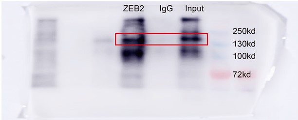
- In Figure 7C, the author claimed to have used 293T cells for the ubiquitin assay, which are not breast cancer cells. Moreover, the efficiency of over-expression differs between ZEB2 and ACSL4 in 293T cell lines. Performing the experiment in an unrelated cell line to justify an important interaction is not acceptable.
Response: We thank the reviewer for the concern. We also performed the ubiquitination assay in MDA-MB-231 cells in Fig 7D (Author response image 2), The results confirm that knockdown of ACSL4 obviously enhanced the ubiqutination of ZEB2. We also have performed the IP experiment in MDA-MB-231 cells in Author response image 3 (Fig 7F). The results confirmed the interaction between ZEB2 and ACSL4:
Author response image 2.
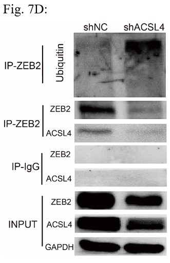
Author response image 3.
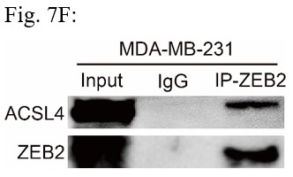
Reviewer #2 (Public Review):
In this study, the authors validated a positive feedback loop between ZEB2 and ACSL4 in breast cancer, which regulates lipid metabolism to promote metastasis.
Overall, the study is original, well structured, and easy to read.
We appreciate the positive comments from the reviewer.
Reviewer #3 (Public Review):
The manuscript by Lin et al. reveals a novel positive regulatory loop between ZEB2 and ACSL4, which promotes lipid droplets storage to meet the energy needs of breast cancer metastasis.
We appreciate the positive comments from the reviewer.
Reviewer #2 (Recommendations For The Authors):
I still have some points that should be addressed by the Authors:
The interaction between ACSL4 and ZEB2 is still not convincing, due to the cellular localization of ACSL4 and ZEB2 is different. The authors should consider utilizing the Duolink experiment to more accurately determine the interaction location of these two proteins in cells.
Response: We appreciate the reviewer’s suggestion. We performed GST pull-down assay to examine whether ZEB2 and ACSL4 form a complex. GST pull-down assay confirmed the interaction of ZEB2 and ACSL4 (Supplementary Fig. S10). We also performed immunofluorescence assay and found that ZEB2 was co-localized with ACSL4 in some certain regions of the cytoplasm in Author response image 5 (Supplementary Fig. S11):
Author response image 4.
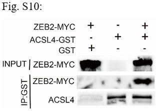
Author response image 5.
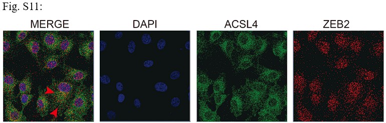
In Figure S4, the authors showed both "shACSL4" and "siACSL4", which is a description error.
Response: We appreciate the reviewer to point out the mistake. We have corrected the "siACSL4" into "shACSL4".
Author response image 6.
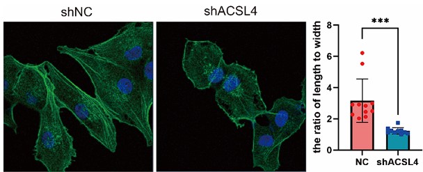
Reviewer #3 (Recommendations For The Authors):
The manuscript is improved.
We appreciate the positive comments from the reviewer.
Author response:
The following is the authors’ response to the previous reviews.
Responses to Reviewer #1:
Reviewer #1: The study shows a new mechanism of NFkB-p65 regulation mediated by Vangl2-dependent autophagic targeting. Autophagic regulation of p65 has been reported earlier; this study brings an additional set of molecular players involved in this important regulatory event, which may have implications for chronic and acute inflammatory conditions.
Comments on the revised version:
The authors have addressed the earlier concerns and I am satisfied with the revised version. I have no additional comments to make.
We appreciate the reviewer’s comments on our revised manuscript.
Responses to Reviewer #2:
Reviewer #2: Vangl2, a core planar cell polarity protein involved in Wnt/PCP signaling, cell proliferation, differentiation, homeostasis, and cell migration. Vangl2 malfunctioning has been linked to various human ailments, including autoimmune and neoplastic disorders. Interestingly, it was shown that Vangl2 interacts with the autophagy regulator p62, and autophagic degradation limits the activity of inflammatory mediators, such as p65/NF-κB. However, the possible role of Vangl2 in inflammation has not been investigated. In this manuscript, Lu et al. describe that Vangl2 expression is upregulated in human sepsis-associated PBMCs and that Vangl2 mitigates experimental sepsis in mice by negatively regulating p65/NF-κB signaling in myeloid cells. Their mechanistic studies further revealed that Vangl2 recruits the E3 ubiquitin ligase PDLIM2 to promote K63-linked poly-ubiquitination of p65. Vangl2 also facilitated the recognition of ubiquitinated p65 by the cargo receptor NDP52. These molecular processes caused selective autophagic degradation of p65. Indeed, abrogation of PDLIM2 or NDP52 functions rescued p65 from autophagic degradation, leading to extended p65/NF-κB activity in myeloid cells. Overall, the manuscript presents convincing evidence for novel Vangl2-mediated control of inflammatory p65/NF-kB activity. The proposed pathway may expand interventional opportunities restraining aberrant p65/NF-kB activity in human ailments.
IKK is known to mediate p65 phosphorylation, which instructs NF-kB transcriptional activity. In this manuscript, Vangl2 deficiency led to an increased accumulation of phosphorylated p65 and IKK also at 30 minutes post-LPS stimulation; however, autophagic degradation of p-p65 may not have been initiated at this early time point. Therefore, this set of data put forward the exciting possibility that Vangl2 could also be regulating the immediate early phase of inflammatory response involving the IKK-p65 axis - a proposition that may be tested in future studies.
We appreciate the reviewer’s comments on our manuscript, and we have added the discussion about IKK-p65 axis in revised version. (Page 15, lines 467-474)
Responses to Reviewer #3:
Reviewer #3: Lu et al. describe Vangl2 as a negative regulator of inflammation in myeloid cells. The primary mechanism appears to be through binding p65 and promoting its degradation, albeit in an unusual autolysosome/autophagy dependent manner. Overall, these findings are novel, valuable and the crosstalk of PCP pathway protein Vangl2 with NF-kappaB is of interest. While generally solid, some concerns still remain about the rigor and conclusions drawn.
Comments on the revised version:
(1) Lu et al. address my comments through responses and new experimental data. However, some of the explanations provided are inadequate.
However, in response to my enquiry regarding directly exploring PCP effects, the authors simply assert "Our study revealed that Vangl2 recruits the E3 ubiquitin ligase PDLIM2 to facilitate K63-linked ubiquitination of p65, which is subsequently recognized by autophagy receptor NDP52 and then promotes the autophagic degradation of p65. Our findings by using autophagy inhibitors and autophagic-deficient cells indicate that Vangl2 regulates NFkB signaling through a selective autophagic pathway, rather than affecting the PCP pathway, WNT, HH/GLI, Fat-Dachsous or even mechanical tension."
I do not agree that the use of autophagy inhibitors and autophagy-deficient cells can rule out the contributions of PCP or any other pathways. Only experimentally inhibiting the pathway(s) with adequate demonstration of target inhibition/abolition of well-known effector function and documenting unaltered p65 regulation under these conditions can be considered proof. Autophagy inhibitors and autophagy-deficient cells only prove that this particular pathway is necessary. Nonetheless, I do not want to dwell on proving a negative and agree that Vangl2 is a novel regulator of p65 through its role in promoting p65 degradation. The inclusion of a statement discussing the limitations of their approach would have sufficed. The response from the authors could have been better.
We thank the reviewer for helping us improve the quality of the manuscript. We provided new data and revised the Discussion as suggested.
To ascertain whether Vangl2 degrades p65 through a selective autophagic pathway or the PCP pathway, 293T cells were transfected with p65, together with or without the Vangl2 plasmids, and treated with different pharmacological inhibitors. We found the degradation of p65 induced by Vangl2 was blocked by autolysosome inhibitor (CQ), but not by the JNK inhibitor (SP600125) or Wnt/β-catenin inhibitor (FH535) (New Figure. 1). These data suggest that Vangl2 primarily degrades p65 through a selective autophagic pathway, rather than through the JNK or Wnt signaling pathway. Nevertheless, additional pathway inhibitions, such as those of the HH/GLI and Fat-Dachsous pathways, should also be employed to further elucidate the function of Vangl2 in p65 degradation. As suggested, we have added a statement about the limitation of the approach in the discussion (Page 12, lines 378-385).
Author response image 1.
Vangl2 degrades p65 through a selective autophagic pathway, but not by the PCP pathway. HEK293T cells were transfected with Flag-p65 and HA-Vangl2 plasmids, and treated with DMSO, CQ (50 mM) for 6 h, SP600125 (20 mM) for 1 h or FH535 (30 mM) for 6 h. The cell lysates were analyzed by immunoblot.
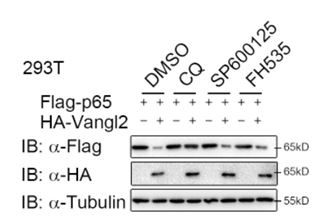
(2) I am also not satisfied with the explanation that "immune cells represent a minor fraction of the lungs and liver". There are lots of resident immune cells in the lungs and liver (alveolar macrophages in the lung and Kuppfer cells in the liver). For example, it may be so that Vangl2 is important in monocytes and not in the resident population. This might be a potential explanation. But this is not explored. The restricted tissue-specificity of the interaction between two ubiquitously present proteins is still a challenge to understand. The response from the authors is not satisfactory. There is plenty of Vangl2 in the liver in their western blot.
We thank the reviewer for this question. We added this explanation in the Discussion. (Page 13, lines 398-404)
(3) I had also simply pointed out PMID: 34214490 with reference to the findings described in the manuscript. There were no suggestions of contradiction. In fact, I would refer to the publication in discussion to support the findings and stress the novelty. The response from the authors could have been better.
Thank you for the reviewer's insightful comments. We have modified this discussion as suggested. (Page 13, lines 410-415; Page 14, lines 419-421)
(4) The response to my enquiry regarding homo- or heterozygosity is unsupported by any reference or data.
As suggested, we provided the data that only Vangl2 deficient homozygous showed inhibition of the activation of NF-kB in New Figure. 2.
Author response image 2.
Vangl2 deficiency promotes NF-kB activation. (A) The survival rates of WT, Vangl2ΔM/ΔM and Vangl2ΔM/WT mice treated with high-dosage of LPS (30 mg/kg, i.p.) (n≥4). (B) IL-6 and TNF-a secretion by WT and Vangl2-deficient BMDMs treated with LPS for 6 h was measured by ELISA. IL-1β secretion by WT, Vangl2ΔM/ΔM and Vangl2ΔM/WT BMDMs treated with LPS for 6 h and ATP for 30 min was measured by ELISA.
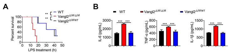
(5) The listing of 8 patients and healthy controls are also appreciated. The body temperature of #6 doesn't fall in the <36 or >38 degree C SIRS criteria. The inclusion of CRP, PCT, heart rate and respiratory rate, and other lab values would have further improved the inclusion criteria. Moreover, it is difficult to understand why there are 16 value points for healthy and sepsis cohorts in Fig 1 when there are 8 patients.
We thank the reviewer for this valuable suggestion. We are sorry for our mistake that we entered data from two repeated experiments in Figure. 1 A and we have revised this data in the updated version (Figure. 1 A, Pages 12 Lines 146). As suggested, we have added CRP, WBC and heart rate in sepsis patients’ information. (Supplementary Materials and Methods)
Recommendations for the authors:
Reviewer #2 (Recommendations For The Authors):
The proposition that Vangl2 may target additional mediators of inflammation could be indicated in the text.
We thank the reviewer for this valuable suggestion. We had added discussion in modified version. (Page 15, lines 467-474)
Reviewer #3 (Recommendations For The Authors):
It is advised that some of the deficiencies pointed out by Reviewer #3 are textually addressed. Additionally, there could be some inconsistency in the number of healthy controls and patients (see Fig S1A and FIg 1A and Supplementary table, also see comments from Reviewer #3) - this should be carefully scrutinised and revised, if necessary.
We thank the reviewer for this valuable suggestion. We are sorry for our mistake that we entered data from two repeated experiments in Figure. 1 A and we have revised this data in the updated version (Figure. 1 A, Pages 12 Lines 146).
Author response:
The following is the authors’ response to the previous reviews
Reviewer #1 (Public review):
Summary:
Audio et al. measured cerebral blood volume (CBV) across cortical areas and layers using high-resolution MRI with contrast agents in non-human primates. While the non-invasive CBV MRI methodology is often used to enhance fMRI sensitivity in NHPs, its application for baseline CBV measurement is rare due to the complexities of susceptibility contrast mechanisms. The authors determined the number of large vessels and the areal and laminar variations of CBV in NHP, and compared those with various other metrics.
Strengths:
Noninvasive mapping of relative cerebral blood volume is novel for non-human primates. A key finding was the observation of variations in CBV across regions; primary sensory cortices had high CBV, whereas other higher areas had low CBV. The measured CBV values correlated with previously reported neuronal and receptor densities.
We appreciate your recognition of the novelty of our non-invasive relative cerebral blood volume (CBV) mapping in non-human primates, as well as the observed areal variations and their correlations with neuronal and receptor densities. However, we are concerned that key contributions of our work—such as cortical layer-specific vasculature mapping and benchmarking surface vessel density estimations against anatomical ground truth—are being framed as limitations rather than significant advances in the field pushing the boundaries of current neuroimaging capabilities and providing a valuable foundation for future research. Additionally, we would like to clarify that dynamic susceptibility contrast (DSC) MRI using gadolinium is the gold standard for CBV measurement in clinical settings and the argument that “baseline CBV measurements are rare due to the complexities of susceptibility contrast” is simply not true. The limited use of ferumoxytol for CBV imaging is primarily due to previous FDA regulatory restrictions, rather than inherent methodological shortcomings.
Changes in text:
Compared to clinically used gadolinium-based agents, ferumoxytol's substantially longer half-life and stronger R<sub>2</sub>* effect allows for higher-resolution and more sensitive vascular volume measurements (Buch et al., 2022), albeit these methodologies are hampered by confounding factors such as vessel orientation relative to the magnetic field (B<sub>0</sub>) direction (Ogawa et al., 1993).
Weaknesses:
A weakness of this manuscript is that the quantification of CBV with postprocessing approaches to remove susceptibility effects from pial and penetrating vessels is not fully validated, especially on a laminar scale. Further specific comments follow.
(1) Baseline CBV indices were determined using contrast agent-enhanced MRI (deltaR<sub>2</sub>*). Although this approach is suitable for areal comparisons, its application at a laminar scale poses challenges due to significant contributions from large vessels including pial vessels. The primary concern is whether large-vessel contributions can be removed from the measured deltaR<sub>2</sub>* through processing techniques.
Eliminating the contribution of large vessels completely is unlikely, and we agree with the reviewer that ΔR<sub>2</sub>* results likely reflect a weighted combination of signals from both large vessels and capillaries. However, the distribution of ΔR<sub>2</sub>* more closely aligns with capillary density in areas V1–V5 than with large vessel distributions (Weber et al., 2008), suggesting that our ΔR<sub>2</sub>* results are more weighted toward capillaries. Moreover, we demonstrated that the pial vessel induced signal-intensity drop-outs are clearly limited to the superficial layers and exhibit smaller spatial extent than generally thought (Supp. Figs. 2 and 4).
(2) High-resolution MRI with a critical sampling frequency estimated from previous studies (Weber 2008, Zheng 1991) was performed to separate penetrating vessels. However, this approach is still insufficient to accurately identify the number of vessels due to the blooming effects of susceptibility and insufficient spatial resolution. The reported number of penetrating vessels is only applicable to the experimental and processing conditions used in this study, which cannot be generalized.
Our intention was not to suggest that our measurements provide a general estimate of vessel density across the macaque cerebral cortex. At 0.23 mm isotropic resolution, we successfully delineated approximately 30% of the penetrating vessels in V1. Our primary objective was to demonstrate a proof-of-concept quantifiable measurement rather than to establish a generalized vessel density metric for all brain regions. We have consistently emphasized this throughout the manuscript, but if there is a specific point of misunderstanding, we would be happy to consider revisions for clarity.
(3) Baseline R<sub>2</sub>* is sensitive to baseline R<sub>2</sub>, vascular volume, iron content, and susceptibility gradients. Additionally, it is sensitive to imaging parameters; higher spatial resolution tends to result in lower R<sub>2</sub>* values (closer to the R<sub>2</sub> value). Thus, it is difficult to correlate baseline R<sub>2</sub>* with physiological parameters.
The observed correlation between R<sub>2</sub>* and neuron density is likely indirect, as R<sub>2</sub>* is strongly influenced by iron, myelin, and deoxyhemoglobin densities. However, the robust correlation between R<sub>2</sub>* and neuron density, peaking in the superficial layers (R = 0.86, p < 10<sup>-10</sup>), is striking and difficult to ignore (revised Supp. Fig. 6D-E). Upon revision, we identified an error in Supp. Fig. 6D-E, where the previous version used single-subject R<sub>2</sub>* and ΔR<sub>2</sub>* maps instead of the group-averaged maps. The revised correlations are slightly stronger than in the earlier version.
Given that the correlation between neuron density and R<sub>2</sub>* is strongest in the superficial layers, we suggest this relationship reflects an underlying association with tissue cytochrome oxidase (CO) activity and cumulative effect of deoxygenated venous blood drainage toward the pial network. The superficial cortical layers are also less influenced by myelin and iron densities, which are more concentrated in the deeper cortical layers. Additional factors may contribute to this relationship, including the iron dependence of mitochondrial CO activity, as iron is an essential component of CO’s heme groups. Moreover, myelin maintenance depends on iron, which is predominantly stored in oligodendrocytes. The presence of myelinated thin axons and a higher axonal surface density may, in turn, be a prerequisite for high neuron density.
In this context, it is also valuable to note the absolute range of superficial R<sub>2</sub>* values (≈ 6 s<sup>-1</sup>; Supp. Fig. 6D). This variation in cortical surface R<sub>2</sub>* is about 12-30 times larger compared to the signal changes observed during task-based fMRI (6 vs. 0.2-0.5 s<sup>-1</sup>). This relation seems reasonable because regional increases in absolute blood flow associated with imaging signals, as measured by PET, typically do not exceed 5%–10% of the brain's resting blood flow (Raichle and Mintum 2016; Brain work and brain imaging). The venous oxygenation level is typically 60%, with task-induced activation increasing it by only a few percent. We suggest that this is ~40% oxygen extraction is reflected in the superficial R<sub>2</sub>*. Finally, the large intercept (≈ 14.5 1/s; Supp. Fig. 6D), which is not equivalent to the water R<sub>2</sub>* (≈ 1 1/s), suggests that R<sub>2</sub>* is influenced by substantial non-neuron density factors, such as receptor, myelin, iron, susceptibility gradients and spatial resolution.
The R<sub>2</sub>* values are well known to be influenced by intra-voxel phase coherence and thus spatial resolution. However, our view is that the proposed methodology of acquiring cortical-layer thickness adjusted high-resolution (spin-echo) R<sub>2</sub> maps poses more methodological limitations and is less practical. Notwithstanding, to further corroborate the relationship between R<sub>2</sub>* and neuron density, we investigated whether a similar correlation exists in non-quantitative T2w SPACE-FLAIR images (0.32 mm isotropic) signal-intensity and neuron density. Using B<sub>1</sub> bias-field and B<sub>0</sub> orientation bias corrected T2w SPACE-FLAIR images (N=7), we parcellated the equivolumetric surface maps using Vanderbilt sections. Our findings showed that signal intensity—where regions with high signal intensity correspond to low R<sub>2</sub> values, and areas with low signal intensity correspond to high R<sub>2</sub> values—was positively correlated with neuron density, particularly in the superficial layers (R = 0.77, p = 10<sup>-11</sup>; Author response image 1).This analysis confirmed the correlation with neuron density and R<sub>2</sub> peaks at superficial layers. However, this correlation was slightly weaker compared to quantitative R<sub>2</sub>* (Supp. Fig. 6D), suggesting the variable flip-angle spin-echo train refocused signal-phase coherence loss from large draining vessels or that non-quantitative T2w-FLAIR images may be confounded by other factors such as B<sub>1</sub> transmission field biases (Glasser et al., 2022). Notwithstanding, this non-quantitative fast spin-echo with variable flip-angles approach, which is in principle less dependent on image resolution and closer to R<sub>2,intrinsic</sub> than R<sub>2</sub>*, yields similar findings in comparison to quantitative gradient-echo.
Author response image 1.
(A) T2w-FLAIR SPACE normalized signal-intensity plotted vs neuron density. Note that low signal-intensity corresponds to high R<sub>2</sub> and high neuron density, consistent with findings using ME-GRE. (B) Correlation between T2w-FLAIR SPACE and neuron density across equivolumetric layers. Notably, a similar relationship with neuron density was observed using a variable spin-echo pulse sequence as with quantitative gradient-echo-based imaging.
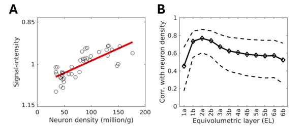
Changes in text:
Results:
“Because the Julich cortical area atlas covers only a section of the cerebral cortex, and the neuron density estimates are interpolated maps, we extended our analysis using the original Collins sample borders encompassing the entire cerebral cortex (Supp. Fig. 6A-C). This analysis reaffirmed the positive correlation with ΔR<sub>2</sub>* (peak at EL2, R = 0.80, p < 10<sup>-11</sup>) and baseline R<sub>2</sub>* (peak at EL2a, R = 0.86, p < 10<sup>-13</sup>), yielding linear coefficients of ΔR<sub>2</sub>* = 102 × 10<sup>3</sup> neurons/s and R<sub>2</sub>* = 41 × 10<sup>3</sup> neurons/s (Supp. Fig. 6D-G). This suggests that the sensitivity of quantitative layer R<sub>2</sub>* MRI in detecting neuronal loss is relatively weak, and the introduction of the Ferumoxytol contrast agent has the potential to enhance this sensitivity by a factor of 2.5.”
A new paragraph was added into discussion section 4.3 corroborating the relation between R<sub>2</sub>* and neuron density:
“Another key finding of this study was the strong correlation between baseline R<sub>2</sub>* and neuron density (Supp. Fig. 6D, E). While R<sub>2</sub>* is well known to be influenced by iron, myelin, and deoxyhemoglobin densities, this correlation peaks in the superficial layers (Supp. Fig. 6E), suggesting a link to CO activity and the accumulation of deoxygenated venous blood draining from all cortical layers toward the pial network. Notably, the absolute range of superficial R<sub>2</sub>* values (max - min ≈ 6 s<sup>-1</sup>; Supp. Fig. 6D) is approximately 12-30 times larger than the ΔR<sub>2</sub>* observed during task-based BOLD fMRI at 3T (0.2-0.5 1/s) (Yablonskiy and Haacke 1994). Since venous oxygenation is around 60% and task-induced changes in blood flow account for only 5%–10% of the brain's resting blood flow (Raichle & Mintun, 2006), these results suggest that superficial R<sub>2</sub>* (Fig. 1D) may serve as a more accurate proxy for total deoxyhemoglobin content (and thus total oxygen consumption), which scales with the neuron density of the underlying cortical gray matter. Importantly, superficial layers may also provide a more specific measure of deoxyhemoglobin, as they are less influenced by myelin and iron, which are more concentrated in deeper cortical layers. Additionally, smaller but direct contributors, such as mitochondrial CO density—an iron-dependent factor—may also play a role in this relationship.”
References:
Raichle, M.E., Mintun, M.A., 2006. BRAIN WORK AND BRAIN IMAGING. Annu. Rev. Neurosci. 29, 449–476. https://doi.org/10.1146/annurev.neuro.29.051605.112819
(4) CBV-weighted deltaR<sub>2</sub>* is correlated with various other metrics (cytoarchitectural parcellation, myelin/receptor density, cortical thickness, CO, cell-type specificity, etc.). While testing the correlation between deltaR<sub>2</sub>* and these other metrics may be acceptable as an exploratory analysis, it is challenging for readers to discern a causal relationship between them. A critical question is whether CBV-weighted deltaR<sub>2</sub>* can provide insights into other metrics in diseased or abnormal brain states.
We acknowledge that having multivariate analysis using dense histological maps would be valuable to establish causality among these several metrics:
“To comprehensively understand the factors contributing to the vascular organization of the brain, experimental disentanglement through multivariate analysis of laminar cell types and receptor densities is needed (Hayashi et al., 2021, Froudist-Walsh et al., 2023). Moreover, employing more advanced statistical modeling, including considerations for synapse-neuron interactions, may be important for refined evaluations.”
We think the primary contributors to the brain's energy budget are neurons and receptors, as shown in several references and stated in the manuscript. To investigate relationship between neuron density and CBV, we estimated the energy budget allocated to neurons and extrapolated the remaining CBV to other contributing factors:
Changes in text:
“However, this is a simplified estimation, and a more comprehensive assessment would need to account for an aggregate of biophysical factors such as neuron types, neuron membrane surface area, firing rates, dendritic and synaptic densities (Fig. 6F-G), neurotransmitter recycling, and other cell types (Kageyama 1982; Elston and Rose 1997; Perge et al., 2009; Harris et al., 2012). Indeed, the majority of the mitochondria reside in the dendrites and synaptic transmission is widely acknowledged to drive the majority of the energy consumption and blood flow (Wong-Riley, 1989; Attwell et al., 2001).
Extrapolating cortical ΔR<sub>2</sub>* to zero neuron density results in a large intercept (~35 1/s), corresponding to 60% of the maximum cortical CBV (57 1/s; Supp. Fig. 6F). This supports the view that the majority of energy consumption occurs in the neuropil—comprising dendrites, synapses, and axons—which accounts for ~80–90% of cortical gray matter volume, whereas neuronal somata constitute only ~10–20% (Wong-Riley, 1989). Although neuronal cell bodies exhibit higher CO activity per unit volume due to their dense mitochondrial content, these results suggest their overall contribution to the total CBV per mm<sup>3</sup> tissue remains lower than that of the neuropil, given the latter's substantially larger volume fraction in cortical tissue.
Contrary to our initial expectations, we observed a relatively smaller CBV in regions and layers with high receptor density (Fig. 6B, D, F). This relationship extends to other factors, such as number of spines (putative excitatory inputs) and dendrite tree size across the entire cerebral cortex (Supp. Fig. 7) (Froudist-Walsh et al., 2023, Elston 2007). These results align with the work of Weber and colleagues, who reported a similar negative correlation between vascular length density and synaptic density, as well as a positive correlation with neuron density in macaque V1 across cortical layers (Weber et al., 2008).”
Variations in neurons and receptors are reflected in cytoarchitecture, myelin (axon density likely scales with neuron density and myelin inhibits synaptic connections), and cell-type composition. For example, fast-spiking parvalbumin interneurons, which target the soma or axon hillock, are well-suited for regulating activity in regions with high neuron density, whereas bursting calretinin interneurons, which target distal dendrites, are more adapted to areas with high synaptic density. These factors in turn, gradually change along the cortical hierarchy level (higher levels have thinner cortical layer IV, more complex dendrite trees and more numerous inter-areal connectivity patterns). In our view, these factors are tightly interlinked and explain the strong correlations and metabolic demands observed across different metrics.
We also agree that cortical layer imaging of vasculature in diseased or abnormal brain states is an intriguing direction for future research; however, it falls beyond the scope of the present study.
Reviewer #2 (Public review):
Summary:
This manuscript presents a new approach for non-invasive, MRI-based, measurements of cerebral blood volume (CBV). Here, the authors use ferumoxytol, a high-contrast agent and apply specific sequences to infer CBV. The authors then move to statistically compare measured regional CBV with known distribution of different types of neurons, markers of metabolic load and others. While the presented methodology captures and estimated 30% of the vasculature, the authors corroborated previous findings regarding lack of vascular compartmentalization around functional neuronal units in the primary visual cortex.
Strengths:
Non invasive methodology geared to map vascular properties in vivo.
Implementation of a highly sensitive approach for measuring blood volume.
Ability to map vascular structural and functional vascular metrics to other types of published data.
Weaknesses:
The key issue here is the underlying assumption about the appropriate spatial sampling frequency needed to captures the architecture of the brain vasculature. Namely, ~7 penetrating vessels / mm2 as derived from Weber et al 2008 (Cer Cor). The cited work, begins by characterizing the spacing of penetrating arteries and ascending veins using vascular cast of 7 monkeys (Macaca mulatta, same as in the current paper). The ~7 penetrating vessels / mm2 is computed by dividing the total number of identified vessels by the area imaged. The problem here is that all measurements were made in a "non-volumetric" manner and only in V1. Extrapolating from here to the entire brain seems like an over-assumption, particularly given the region-dependent heterogeneity that the current paper reports.
We appreciate the reviewer’s concerns regarding spatial sampling frequency and its implications for characterizing brain vasculature, which we investigated in this study. To clarify, our analysis of surface vessel density was explicitly restricted to V1 precisely due to the limitations of our experimental precision. While we reported the total number of vessels identified in the cortex, we intentionally chose not to present density values across regions in this manuscript. Although these calculations are feasible, we focused on the data directly analyzed and avoided extrapolating density values beyond the scope of our findings. Thus, we are uncertain about the suggestion that we extrapolated vessel density values across the entire brain, as we have taken care to limit our conclusions of our vessel density precision to V1.
Regarding methodology, we conducted two independent analyses of vessel density specifically in V1. The first involved volumetric analysis using the Frangi filter, while the second used surface-based analysis of local signal-intensity gradients (as illustrated in Fig. 2E and Supp. Figs. 3 and 4), albeit the final surface density analysis is performed using the ultra-high resolution equivolumetric layers. Notably, these two approaches produced consistent and comparable vessel density estimates, supporting the reliability of our findings within the scope of V1 (we found 30% of the vessels relative to the ground-truth).
Comments on revisions:
I appreciate the effort made to improve the manuscript. That said, the direct validation of the underlying assumption about spatial resolution sampling remains unaddressed in the final version of this manuscript. With the only intention to further strengthen the methodology presented here, I would encourage again the authors to seek a direct validation of this assumption for other brain areas.
In their reply, the authors stated "... line scanning or single-plane sequences, at least on first impression, seem inadequate for whole-brain coverage and cortical surface mapping. ". This seems to emanate for a misunderstanding as the method could be used to validate the mapping, not to map per-se.
We apologize for any misunderstanding in our previous response and appreciate your clarification. We now understand that you were suggesting the use of line-scanning or single-plane sequences as a method to validate, rather than map, our spatial sampling assumptions.
We agree that single-plane sequences at very high in-plane resolution (e.g., 50 × 50 × 1000 µm) have great potential to detect penetrating vessels and even vessel branching patterns. These techniques could indeed provide valuable insights into region-specific vessel density variations which could then be used to validate whole brain 3D acquisitions. However, as noted above, we have refrained from reporting vessel densities outside V1 precisely due to sampling limitations (we only found 30% of the penetrating vessels in V1, or only 2 mm<sup>2</sup>/30mm<sup>2</sup> ≈ 7% of branching vessel ground-truth, see discussion).
We acknowledge the merit of incorporating such methods to validate regional vessel densities and agree that this would be an important avenue for future research. Thank you for suggesting this point, we have briefly mentioned the advantage of single-plane EPI at discussion.
Changes in text:
“4.1 Methodological considerations - vessel density informed MRI
…anatomical studies accounting for branching patterns have reported much higher vessel densities up to 30 vessels/mm<sup>2</sup> (Keller et al., 2011; Adams et al., 2015). Further investigations are warranted, taking into account critical sampling frequencies associated with vessel branching patterns (Duverney 1981), and achieving higher SNR through ultra-high B<sub>0</sub> MRI (Bolan et al., 2006; Harel et al., 2010; Kim et al., 2013) and utilize high-resolution single-plane sequences and prospective motion correction schemes to accurately characterize regional vessel densities. Such advancements hold promise for improving vessel quantification, classifications for veins and arteries and constructing detailed cortical surface maps of the vascular networks which may have diagnostic and neurosurgical utilities (Fig. 2A, B) (Iadecola, 2013; Qi and Roper, 2021; Sweeney et al., 2018).”
During the revision we found a typo and corrected it in Supp. Fig. 8: Dosal -> Dorsal.
Author response:
The following is the authors’ response to the original reviews.
In light of some reviewer comments requesting more clarity on the relationship between our model and prior theoretical studies of systems consolidation, we propose a modification to the title of our manuscript: “Selective consolidation of learning and memory via recall-gated plasticity.” We believe this title better reflects the key distinguishing feature of our model, that it selectively consolidates only a subset of memories, and also highlights the model’s applicability to task learning as well as memory storage.
Major comments:
Reviewer #3’s primary concern with the paper is the following: “The main weakness of the paper is the equation of recall strength with the synaptic changes brought about by the presentation of a stimulus. In most models of learning, synaptic changes are driven by an error signal and hence cease once the task has been learned. The suggested consolidation mechanism would stop at that point, although recall is still fine. The authors should discuss other notions of recall strength that would allow memory consolidation to continue after the initial learning phase.”
We thank the reviewer for drawing attention to this issue, which primarily results from a poor that memories should be interpreted as actual synaptic weight updates,∆𝑤and thus in the context choice of notation on our part. Our decision to denote memories as gives the impression of supervised learning would go to zero when the task is learned. However, in the formalism of our model, memories are in fact better interpreted as target values of synaptic weights, and the synaptic model/plasticity rule is responsible for converting these target values into synaptic weight updates. We were unclear on this point in our initial submission, because our paper primarily considers binary synaptic weights, where target synaptic weights have a one-to-one correspondence with candidate synaptic weight updates. We have updated the paper to use w* to refer to memories, which we hope resolves this confusion, and have updated our introduction to the term “memory” to reflect their interpretation as target synaptic weight values. We have also updated the paper’s language to more clearly disambiguate between the “learning rule,” which determines how the memory vector (target synaptic weight vectors) are derived from task variables, and the “plasticity rule,” which governs how these are translated into actual synaptic weight updates. We acknowledge that our manuscript still does not explicitly consider a plasticity rule that is sensitive to continuous error error signals, as our analysis is restricted to binary weights. However, we believe that the updated notation and exposition makes it more clear that our model could be applied in such a case.
Reviewer #1 brought up that our framework cannot capture “single-shot learning, for example, under fear conditioning or if a presented stimulus is astonishing.” Reviewer #2 raised a related question of how our model “relates to the opposite more intuitive idea, that novel surprising experiences should be stored in memory, as the familiar ones are presumably already stored.”
We agree that the built-in inability to consolidate memories after a single experience is a limitation of our model, and that extreme novelty is one factor (among others, such as salience or reward) that might incentivize one-shot consolidation. We have added a comment to the discussion to acknowledge these points (added text in bold): “ Moreover, in real neural circuits, additional factors besides recall, such as reward or salience, are likely to influence consolidation as well. For instance, a sufficiently salient event should be stored in long-term memory even if encountered only once. Furthermore, while in our model familiarity drives consolidation, certain forms of novelty may also incentivize consolidation, raising the prospect of a non-monotonic relationship between consolidation probability and familiarity.” We agree that future work should address the combined influence of recall (as in our model) and other factors on the propensity to consolidate a memory.
Reviewer #1 requested, “a comparison/discussion of the wide range of models on synaptic tagging for consolidation by various types of signals. Notably, studies from Wulfram Gerstner's group (e.g., Brea, J., Clayton, N. S., & Gerstner, W. (2023). Computational models of episodic-like memory in food-caching birds. Nature Communications, 14(1); and studies on surprise).”
We thank the reviewer for the reference, which we have added to the manuscript. The model of Brea et al.(2023) is similar to that of Roxin & Fusi (2013), in that consolidation consists of “copying” synaptic weights from one population to another. As a result, just like the model of Roxin & Fusi (2013), this model does not provide the benefit that our model offers in the context of consolidating repeatedly recurring memories. However, the model of Brea et al. does have other interesting properties – for instance, it affords the ability to decode the age of a memory, which our model does not. We have added a comment on this point in the subsection of the Discussion tilted “Other models of systems consolidation.”
Reviewer #2 noted, “While the article extensively discusses the strengths and advantages of the recall-gated consolidation model, it provides a limited discussion of potential limitations or shortcomings of the model, such as the missing feature of generalization, which is part of previous consolidation models. The model is not compared to other consolidation models in terms of performance and how much it increases the signal-to-noise ratio.”
We agree that our work does not consider the notion of generalization and associated changes to representational geometry that accompany consolidation, which is the focus of many other studies on consolidation. We have further highlighted this limitation in the discussion. Regarding the comparison to other models, this is a tricky point as the desiderata we emphasize in this study (the ability to recall memories that are intermittently reinforced) is not the focus of other studies. Indeed, our focus is primarily on the ability of systems consolidation to be selective in which memories are consolidated, which is somewhat orthogonal to the focus of many other theoretical studies of consolidation. We have updated some wording in the introduction to emphasize this focus.
Additional comments made by reviewer #1
Reviewer #1 pointed out issues in the clarity of Fig. 2A. We have added substantial clarifying text to the figure caption.
Reviewer #1 pointed out lack of clarity in our introduction to the terms “reliability” and “reinforcement.” We have now made it more clear what we mean by these terms the first time they are used.
We have updated our definition of “recall” to use the term “recall factor,” which is how we refer to it subsequently in the paper.
We have made explicit in the main text our simplifying assumption that memories are mean-centered.
We have made consistent our use of “forgetting curve” and “memory trace”.
Additional comments made by reviewer #2
We have added a comment in the discussion acknowledging alternative interpretations of the result of Terada et al. (2021)
We have significantly expanded the discussion of findings about the mushroom body to make it accessible to readers who do not specialize in this area. We hope this clarifies the nature of the experimental finding, which uncovered a circuit that performs a strikingly clean implementation of our model.
The reviewer expresses concern that the songbird study (Tachibana et al., 2022) does not provide direct evidence for consolidation being gated by familiarity of patterns of activity. Indeed, the experimental finding is one-step removed from the direct predictions of our model. That said, the finding – that the rate of consolidation increases with performance – is highly nontrivial, and is predicted by our model when applied to reinforcement learning tasks. We have added a comment to the discussion acknowledging that this experimental support for our model is behavioral and not mechanistic.
We do not regard it as completely trivial that the parallel LTM model performs roughly the same as the STM model, since a slower learning rate can achieve a higher SNR (as in Fig. 2C). Nevertheless we have added wording to the main text around Fig. 4B to note that the result is not too surprising.
We have added a sentence that clarifies the goal / question of our paper earlier on in the introduction.
We have updated Figure 3 by labeling the key components of the schematics and adding more detail to the legend, as suggested by the reviewer. We also reordered the figure panels as suggested.
Additional comments made by reviewer #3:
We have clarified in the main text that Fig. 2C and all results from Fig. 4 onward are derived from an ideal observer model (which we also more clearly define).
We have now emphasized in the main text that the derivations of the recall factors for specific learning rules are derived in the Supplementary Information.
We have highlighted more clearly in the main text that the recall factors associated with specific learning rules may correspond to other notions that do not intuitively correspond to “recall,” and have added a pointer to Fig. 3A where these interpretations are spelled out.
We have added references corresponding to the types of learning rules we consider.
The cutoffs / piecewise-looking behavior of plots in Fig. 4 are primarily the result of finite N, which limits the maximum SNR of the system, rather than coarse sampling of parameter values.
Thank you for pointing out the error in the legend in Fig. 5D (also affected Supp Fig. S7/S8), which is now fixed.
The reference to the nonexistence panel Fig. 5G has been removed.
As the reviewer points out, the use of a binary action output in our reinforcement learning task renders it quite similar to the supervised learning task, making the example less compelling. In the revised manuscript we have updated the RL simulation to use three actions. Note also that in our original submission the network outputs represented action probabilities directly (which is straightforward to do for binary actions, but not for more than two available actions). In order to parameterize a policy when more than two actions are available, we sample actions using a softmax policy, as is more standard in the field and as the reviewer suggested. The associated recall factor is still a product of reward and a “confidence factor,” and the confidence factor is still the value of the network output in the unit corresponding to the chosen action, but in the updated implementation this factor is equal to  , similar (though with a sign difference) to the reviewer’s suggestion. We believe these updates make our RL implementation and simulation more compelling, as it allows them to be applied to tasks with arbitrary numbers of actions.
Additional minor comments
The reviewers made a number of other specific line-by-line wording suggestions, typo corrections,
Author response:
The following is the authors’ response to the original reviews.
eLife assessment
The study provides potentially fundamental insight into the function and evolution of daily rhythms. The authors investigate the function of the putative core circadian clock gene Clock in the cnidarian Nematostella vectensis. While it parts still incomplete, the evidence suggests that, in contrast to mice and fruit flies, Clock in this species is important for daily rhythms under constant conditions, but not under a rhythmic light/dark cycle, suggesting that the major role of the circadian oscillator in this species could be a stabilizing function under non-rhythmic environmental conditions.
Public Reviews:
Reviewer #1 (Public Review):
In this nice study, the authors set out to investigate the role of the canonical circadian gene Clock in the rhythmic biology of the basal metazoan Nematostella vectensis, a sea anemone, which might illuminate the evolution of the Clock gene functionality. To achieve their aims the team generated a Clock knockout mutant line (Clock-/- ) by CRISPR/Cas9 gene deletion and subsequent crossing. They then compared wild-type (WT) with Clock-/- animals for locomotor activity and transcriptomic changes over time in constant darkness (DD) and under light/dark cycles to establish these phenotypes under circadian control and those driven by light cycles. In addition, they used Hybridization Chain Reaction-In situ Hybridization (HCR-ISH) to demonstrate the spatial expression of Clock and a putative circadian clocl-controlled gene Myh7 in whole-mounted juvenile anemones.
The authors demonstrate that under LD both WT and Clock-/- animals were behaviourally rhythmic but under DD the mutants lost this rhythmicity, indicating that Clock is necessary for endogenous rhythms in activity. With altered LD regimes (LD6:6) they show also that Clock is light-dependent. RNAseq comparisons of rhythmic gene expression in WT and Clock-/- animals suggest that clock KO has a profound effect on the rhythmic genome, with very little overlap in rhythmic transcripts between the two phenotypes; of the rhythmic genes in both LD and DD in WT animals (220- termed clock-controlled genes, CCGS) 85% were not rhythmic in Clock-/- animals in either light condition. In silico gene ontology (GO) analysis of CCGS reflected process associated with circadian control. Correspondingly, those genes rhythmic in KO animals under DD (here termed neoCCGs) were not rhythmic in WT, lacked upstream E-box motifs associated with circadian regulation, and did not display any GO enrichment terms. 'Core' circadian genes (as identified in previous literature) in WT and Clock-/- animals were only rhythmic under entrainment (LD) conditions whilst Clock-/- displayed altered expression profiles under LD compared to WT. Comparing CCGs with previous studies of cycling genes in Nematostellar, the authors selected a gene from 16 rhythmic transcripts. One of these, Myh7 was detectable by both RNAseq and HCR-ISH and considered a marker of the circadian clock by the authors.
The authors claim that the study reveals insights into the evolutionary origin of circadian timing; Clock is conserved across distant groups of organisms, having a function as a positive regulator of the transcriptional translational feedback loop at the heart of daily timing, but is not a central element of the core feedback loop circadian system in this basal species. Their behavioural and transcriptomic data largely support the claims that Clock is necessary for endogenous daily activity but that the putative molecular circadian system is not self-sustained under constant darkness (this was known already for WT animals)- rather it is responsive to light cycles with altered dynamics in Clock-/- specimens in some core genes under LD. In the main, I think the authors achieved their aims and the manuscript is a solid piece of important work. The Clock-/- animal is a useful resource for examining time-keeping in a basal metazoan.
The work described builds on other transcriptomic-based works on cnidaria, including Nematostellar, and does probe into the molecular underpinnings with a loss-of-function in a gene known to be core in other circadian systems. The field of chronobiology will benefit from the evolutionary aspect of this work and the fact that it highlights the necessity to study a range of non-model species to get a fuller picture of timing systems to better appreciate the development and diversity of clocks.
Strengths:
The generation of a line of Clock mutant Nematostellar is a very useful tool for the chronobiological community and coupled with a growing suite of tools in this species will be an asset. The experiments seem mostly well conceived and executed (NB see 'weaknesses'). The problem tackled is an interesting one and should be an important contribution to the field.
Weaknesses:
I think the claims about shedding light on the evolutionary origin of circadian time maintenance are a little bold. I agree that the data do point to an alternative role for Clock in this animal in light responsiveness, but this doesn't illuminate the evolution of time-keeping more broadly in my view. In addition, these are transcriptomic data and so should be caveated- they only demonstrate the expression of genes and not physiology beyond that. The time-course analysis is weakened by its low resolution, particularly for the RAIN algorithm when 4-hour intervals constrain the analysis. I accept that only 24h rhythms were selected in the analysis from this but, it might be that detail was lost - I think a preferred option would be 2 or 3-hour resolution or 2 full 24h cycles of analysis.
The authors discount the possibility of the observed 12h rhythmicity in Clock-/- animals by exposing them to LD6:6 cycles before free-running them in DD. I suggest that LD cycles are not a particularly robust way to entrain tidal animals as far as we know. Recent papers show inundation/mechanical agitation are more reliable cues (Kwiatkowski ER, et al. Curr Biol. 2023, 2;33(10):1867-1882.e5. doi: 10.1016/j.cub.2023.03.015; Zhang L., et al Curr Biol. 2013, 23;19, 1863-1873 doi.org/10.1016/j.cub.2013.08.038.) and might be more effective in revealing endogenous 12h rhythms in the absence of 24h cues.
Response: We removed the suggestion that we used 6:6h LD to perform tidal entrainment. We generated this ultradian light condition to address the 24h rhythmicity observed in the NvClk1-/- in 12:12h LD.
Reviewer #2 (Public Review):
This manuscript addresses an important question: what is the role of the gene Clock in the control of circadian rhythms in a very primitive group of animals: Cnidaria. Clock has been found to be essential for circadian rhythms in several animals, but its function outside of Bilaterian animals is unknown. The authors successfully generated a severe loss-of-function mutant in Nematostella. This is an important achievement that should help in understanding the early evolution of circadian clocks. Unfortunately, this study currently suffers from several important weaknesses. In particular, the authors do not present their work in a clear fashion, neither for a general audience nor for more expert readers, and there is a lack of attention to detail. There are also important methodological issues that weaken the study, and I have questions about the robustness of the data and their analysis. I am hoping that the authors will be able to address my concerns, as this work should prove important for the chronobiology field and beyond. I have highlighted below the most important issues, but the manuscript needs editing throughout to be accessible to a broad audience, and referencing could be improved.
Major issues:
(1) Why do the authors make the claim in the abstract that CLOCK function is conserved with other animals when their data suggest that it is not essential for circadian rhythms? dCLK is strictly required in Drosophila for circadian rhythms. In mammals, there are two paralogs, CLOCK and NPAS2, but without them, there are no circadian rhythms either. Note also that the recent claim of BMAL1-independent rhythms in mammals by Ray et al., quoted in the discussion to support the idea that rhythms can be observed in the absence of the positive elements of the circadian core clock, had to be corrected substantially, and its main conclusions have been disputed by both Abruzzi et al. and Ness-Cohn et al. This should be mentioned.
Response: According to our Behavioral and Transcriptomic data, CLOCK function is conserved in constant light condition. In LD context, the rhythmicity is maintained probably by the light-response pathway in Nematostella. We modified our rhythmic transcriptomic analysis and considered the context of the contested results by Ray et al., and discussed it in the revised manuscript.
(2) The discussion of CIPC on line 222 is hard to follow as well. How does mRNA rhythm inform the function of CIPC, and why would it function as a "dampening factor"? Given that it is "the only core clock member included in the Clock-dependent CCGs," (220) more discussion seems warranted. Discussing work done on this protein in mammals and flies might provide more insight.
Response: The initial sentence was unclear. Furthermore, since we restricted our rhythmic analysis to genes only found rhythmic with a p<0.01 with RAIN combined with JTK, NvCipc was no longer defined as rhythmic in free running.
(3) The behavioral arrhythmicity seen with their Clock mutation is really interesting. However, what is shown is only an averaged behavior trace and a single periodogram for the entire population. This leaves open the possibility that individual animals are poorly synchronized with each other, rather than arrhythmic. I also note that in DD there seem to be some residual rhythms, though they do not reach significance. Thus, it is also possible that at least some individual animals retain weak rhythms. The authors should analyze behavioral rhythms in individual animals to determine whether behavioral rhythmicity is really lost. This is important for the solidity of their main conclusions.
Response: Fig. 1 has been modified. We have separated the data for WT and NvClk1-/- animals to provide clarity on the average behavior pattern for each genotype. While the LSP analysis on the population average informs us about the synchronization of the population, it is true that it does not provide insight into individual rhythmicity. To address this, we analyzed individuals in all conditions using the Discorhythm website (Carlucci et al., 2019).
In the revised figure, we have included a comparison plot of the acrophase of 24-hour rhythmic animals between genotypes using Cosinor analysis, which is most suitable for acrophase detection. This plot indicates the number of animals detected as significantly rhythmic, providing direct visual input to the reader regarding individual rhythmicity. Additionally, we have added Table 1, which contains the Cosinor period analysis (24 and 12 hours) of individuals for all genotypes and conditions, further enhancing the clarity of our findings.
(4) There is no mention in the results section of the behavior of heterozygotes. Based on supplement figure 2A, there is a clear reduction in amplitude in the heterozygous animals. Perhaps this might be because there is only half a dose of Clock, but perhaps this could be because of a dominant-negative activity of the truncated protein. There is no direct functional evidence to support the claim that the mutant allele is nonfunctional, so it is important to discuss carefully studies in other species that would support this claim, and the heterozygous behavior since it raises the possibility that the mutant allele acts as a dominant negative.
Response: Extended Data Fig.1 modified. We show NvClk1+/- normalized locomotion over time in DD of the population, comparison of individual normalized behavior amplitude, LSP of the average population and individual acrophase of only rhythmic 24h individuals. Indeed, we cannot discriminate Dominant-negative from non-functional allele.
(5) I do not understand what the bar graphs in Figure 2E and 3B represent - what does the y-axis label refer to?
Response: Not relevant to the revised manuscript.
(6a) I note that RAIN was used, with a p<0.05 cut-off. I believe RAIN is quite generous in calling genes rhythmic, and the p-value cut-off is also quite high. What happens if the stringency is increased, for example with a p<0.01.
Response: We acknowledge your concern regarding the stringency of our statistical analysis. To address this, we opted to combine both RAIN and JTK methods and applied a more stringent p-value cut-off of p<0.01.
(6b) It would be worth choosing a few genes called rhythmic in different conditions (mutant or wild-type. LD or DD), and using qPCR to validate the RNAseq results. For example, in Figure 3D, Myh7 RNAseq data are shown, and they do not look convincing. I am surprised this would be called a circadian rhythm. In wild-type, the curve seems arrhythmic to me, with three peaks, and a rather large difference between the first and second ZT0 time point. In the Clock mutants, rhythms seem to have a 12hr period, so they should not be called rhythmic according to the material and methods, which says that only ca 24hr period mRNA rhythms were considered rhythmic. Also, the result section does not say anything about Myh7 rhythms. What do they tell us? Why were they presented at all?
Response: Regarding the suggestion for independent verification of our RNAseq results, we agree that such validation would enhance the robustness of our findings. To address this, we chose to overlap our identified rhythmic genes under WT LD conditions with those from another transcriptomic study that shared similarities in experimental design. Notably, the majority of overlapping rhythmic genes between the studies are candidate pacemaker genes. We believe that this replication of biologically significant rhythmic genes strengthens the validity and reliability of our results (see Extended Data Fig. 2).
Furthermore, we have decided to remove the NvMhc-st (mistakenly named Myh7, only rhythmic in WT DD in the new analysis) as it does not contribute substantively to the revised version of the manuscript.
(7) The authors should explain better why only the genes that are both rhythmic in LD and DD are considered to be clock-controlled genes (CCGs). In theory, any gene rhythmic in DD could be a CCG. However, Leach and Reitzel actually found that most genes in DD1 do not cycle the next day (DD2)? This suggests that most "rhythmic" genes might show a transient change in expression due to prolonged obscurity and/or the stress induced by the absence of a light-dark cycle, rather than being clock controlled. Is this why the authors saw genes rhythmic under both LD and DD as actual CCGs? I would suggest verifying that in DD the phase of the oscillation for each CCG is similar to that in LD. If a gene is just responding to obscurity, it might show an elevated expression at the end of the dark period of LD, and then a high level in the first hours of DD. Such an expression pattern would be very unlikely to be controlled by the circadian clock.
Response: As we modified our transcriptomic analysis, we do no longer analyze LD+DD rhythmic genes, but any genes rhythmic (RAIN and JTK p<0.01) in each condition. As such we end up with four list of genes corresponding to each experimental conditions.
(8) Since there are still rhythms in LD in Clock mutants, I wonder whether there is a paralog that could be taking Clock's place, similar to NPAS2 in mammals.
Response: see response to (1) > The only NPAS2 orthologous identified in Nematostella NPAS3 showed marginally significance (p=0.013) with RAIN in LD WT suggesting a regulation similar to the candidate pacemaker genes. As such we included within our candidate pacemaker genes list.
(9) I do not follow the point the authors try to make in lines 268-272. The absence of anticipatory behavior in Drosophila Clk mutants results from disruption of the circadian molecular clock, due to the loss of Clk's circadian function. Which light-dependent function of Clock are the authors referring to, then? Also, following this, it should be kept in mind that clock mutant mice have a weakened oscillator. The effect on entrainment is secondary to the weakening of the oscillator, rather than a direct effect on the light input pathway (weaker oscillators have increased response to environmental inputs). The authors thus need to more clearly explain why they think there is a conservation of circadian and photic clock function.
Response: Following the changes in our statistical analysis we reframed the discussion and address directly the circadian and the photic clock function (we call it light-response pathway in the manuscript)
Recommendations for the authors:
We suggest the following improvements:
(1) Please undertake a serious effort to make this work more accessible to non-marine chronobiologists. This includes better explanations, and schemes of the animal when images of staining are shown (e.g. Fig.1b) which include the labeling of relevant morphological structures mentioned in the text (like "tentacle endodermis and mesenteries" (line 132)). Similar issues for mentioned life cycle stages like "late planula stage" (line 133), "bisected physa" (line 149).
Response: Fig. 1b, we outlined the animal shaped and added 2 arrows to locate the tentacle endodermis and mesenteries. We replaced the term late planula stage, by larvae. And we rephrased bisected physa by tissue sampling.
Please attend to details. This includes:
- Wrong referrals to figures (currently line 151 refers to EDF2- but should be EDF 1 instead, there is a Fig.3f mentioned in the text, but there is no such Fig.).
Response: Fixed
- Mentioning of ZTs when the HCR stainings were performed.
Response: Fixed
- Fig.1 a shows a rather incomplete and thus potentially confusing phylogenetic tree. Vertebrates have at least two Clk orthologs (NPAS2 and CLK), please include both, use an outgroup, and rout the tree.
Response: Identifying NPAS2 and CLK orthologous in all species added more confusion into the conclusion. However, we followed the suggestion of adding an outgroup using a CLK orthologous sequence identified in the sponge Amphimedon queenslandica and rout the tree. Thank for the suggestion.
- What do the y-axis labels in Figure 2E and 3B refer to exactly? Y-axis label annotations in Fig.3a,d are entirely missing- what do the numbers refer to?
Response: not relevant in the revised manuscript
- Fig.2D- is the Go term enrichment referring to LD or DD?
Response: to DD. We made it cleared on the figure 5.
- Wording: "Clock regulates genetic pathways." What is meant by "genetic pathways"? There are no "non-genetic pathways". Could one simply say: "Clock regulates a variety of transcripts".
Response: We modified our threshold to use only p.adj<0.01, which reduced the GO term numbers. We removed “genetic pathways” and now address the specific pathways: cell-cycle and neuronal.
The use of the term "epistatic" is confusing (line 219), i.e. that light is epistatic to Clock. In genetics, epistasis is defined as the effect of gene interactions on phenotypes. To a geneticist, this implies that there is a second gene impacting on the phenotype of the Clock mutants. Please re-word.
Response: “light is epistatic on Clock” has been re-phrased.
The provided Supplementary tables are not well annotated. Several of them need guess-work about what is shown. For instance, for Supplementary Table 1, the Ns are unclear, which in total can go up to almost 200 per condition-genotype, but only about 30 animals for each were tested. Thus, where do the high totals in the LSP table come from? What do the numbers of each periodicity mean? Initially one might assume it was the number of animals that showed a periodogram peak at a given periodicity, but it seems that cannot be. Maybe it counted any period bin over statistical significance? Please clarify with better descriptions and labels.
Response: Supplementary tables are now clearly annotated on their first Tabs. About Fig.1, we already addressed this point in the public review.
Albeit not essential, it would be more reader-friendly to also add a summary table with average period and SD, power and SD, and percentage rhythmicity to the main figure.
Response: Table 1 is added: it contains individual count of rhythmic animals (24h and 12h) with Cosinor. However, using Discorhythm we had to ask for a specific Period. Thus, we can only provide animal count significant for a given period value. And not an estimation of their own period.
(2) Some of the terminology is quite confusing, in particular the double meaning of the word "clock" (i.e the pacemaker and the transcription factor). This is not a specific problem to this manuscript, but it would be helpful for the readability to try to improve this.
Could the gene/transcript/protein be spelled: clk and Clk?
Alternatively, for clarity- how about talking about "core pacemaker genes," "CLOCK-dependent rhythmic genes" and "CLOCK-independent rhythmic genes"?
Response:
Clock/CLOCK > NvClk / NvCLK and the mutant is NvClk1-/-
Core clock genes > candidate pacemaker genes.
CLOCK-dependent CCG > this notion no longer exists in the revised manuscript.
CLOCK-independent CCG > this notion no longer exists in the revised manuscript.
(3) The dismissal of the 12h rhythmicity in Clock-/- animals is not really convincing and should be reconsidered. LD6:6 cycles (before free-running animals in DD) is likely a not particularly robust way to entrain tidal animals. Recent papers show inundation/mechanical agitation are more reliable cues (Kwiatkowski ER, et al. Curr Biol. 2023, 2;33(10):1867-1882.e5. doi: 10.1016/j.cub.2023.03.015; Zhang L., et al Curr Biol. 2013, 23;19, 1863-1873 doi.org/10.1016/j.cub.2013.08.038.) and might be more effective in revealing endogenous 12h rhythms in the absence of 24h cues.
Response: We removed the proposition of using 6:6hLD as Tidal entrainment. Instead, the LD 6:6 experiment reveals the direct light-dependency of the NvClk1-/- mutant.
(4) There are significant questions raised on the validity of BMAL1-independent rhythms in mammals as suggested by the Ray et al study. See DOI: 10.1126/science.abe9230 and DOI: 10.1126/science.abf0922
These technical comments should also be taken into account and the discussion adjusted accordingly to better reflect the ongoing discussions in the chronobiology field.
Response: We modified our rhythmic analysis. As we cannot use BHQ or adjusted p-value which resulted in very genes, we defined 24h-rhythmic genes if p<0.01 with two different algorithms (RAIN and JTK). We propose this compromise to reduce the risk of false-positive. Furthermore, we discussed our methodology in the light of the significant questions raised by these papers you cited. We thank the reviewer for this important point.
(5) The HCR stainings for clk are not very convincing. Normally, HCR should have more dots. In principle, the logic of HCR is such that it detects individual mRNA molecules in the cell. Thus, having only one strong dot/cell like in Fig.1b doesn't make much sense.
Response: We were the first surprised by this single dot signal. We are experienced users of HCRv.3 across different species. We decided to remove the close-up (for further investigations) but to keep the full animal signal. According to our approach it is a convincing signal. However, the doty nature of the signal itself it is not easy to make it highly visible at full scale animal on the picture. We did our best to show the mRNA signal visible without altering the pattern.
Furthermore, the controls for the HCR in situ hybridization are unclear. In the methods, there are two Clock probes described (B3 & B5) and two control probes (B1 & B3), however, in the negative control image, a combination of one Clock (B1) and one control (B3) probes is used and is unclear what "redundant detection" means in the legend of figure S2.
Response: Considering the nature of the signal (single of few dots), we decided to use two probes with 2 different fluorophores. A noise is by nature random. Our hypothesis was: only overlapping fluorescent dots are true signal of NvClk mRNA.
For Control probes we used two zebrafish probes labelling hypothalamic peptides.
Based on the experience with non-Drosophila, non-mouse animal model systems the reviewers assume that non-sense mediated mRNA decay (NMD) is not strongly initiated upon Crispr-induced premature STOP-codons. If this assumption is correct it would be worth to mention it. Alternatively, it would be worth testing if Nematostella induces NMD, as this would be a great control for the HCR and the mutation itself. At which ZT was the HCR done?
Response: We performed the HCR at ZT10 when NvClk is described to be at peak. It is now indicated in the Fig. 1b. The RNAseq detected a higher quantity of NvClk1 mRNA in the NvClk1-/- (see Fig. 4a). mRNA quantity regulation involves transcription, stabilization, and degradation. At this stage, we cannot identify which specific step is affected.
For Fig.1c- please provide the binding site and sequence in the figure, simply include EDF 1 in the main figure.
Response: We generated a clear indication in the new Fig.1c and EDF. 1b about the protein domains, the CRISPR binding site and the consequences on the DNA and AA sequences.
(6) Please provide the individual trace data for the behavioral analyses either as supplementary files or as a link to an openly accessible database like DRYAD (see also comment 7 in the public review of reviewer 2). Maybe this is what is shown in Supplementary Table 1, but it is really not clear what is actually shown.
Response: Fig.1 is updated. Table 1 is added. Supplementary Table 1 contains individual normalized locomotor data of each polyps for each genotypes and light conditions. Supplementary Table 2 contains the cosinor individual rhythmic behavior analysis based on the Supplementary Table 1.
(7) It is not really clear if the mutation is a true loss-of-function or could also be dominant negative. While this is raised in the discussion, it should be more carefully considered. The reason why a dominant negative would be unlikely is unclear. More specifically also see comment 8) in the public review of reviewer 2.
Response: Indeed, the results cannot tell us if it is a true loss of function, a dominant negative or non-functional allele. We addressed it in the first part of the discussion.
(8) The pretty small overlap of rhythmic transcripts in LD and DD could reflect the true biology of a more core clock driven-process under constant conditions and a more light-driven process under LD. But still- wouldn't one expect that similar processes should be rhythmic? If not, why not?
It would certainly add strength to the data if for one or two transcripts these results were independently verified by qPCR from an independent sampling. This could even be done for just two time points with the most extreme differences.
Response: We appreciate the reviewer's comments and concerns regarding the overlap of rhythmic transcripts in different conditions. In response to the reviewer's query, we revised our interpretation of the transcriptomic data, acknowledging the limited overlap between light and genotype conditions in our study. This prompted us to reconsider the underlying biological processes driving rhythmic gene expression under constant conditions versus light-dark cycles.
Regarding the suggestion for independent verification of our RNAseq results, we agree that such validation would enhance the robustness of our findings. To address this, we chose to overlap our identified rhythmic genes under WT LD conditions with those from another transcriptomic study that shared similarities in experimental design. Notably, the majority of overlapping rhythmic genes between the studies are candidate pacemaker genes. We believe that this replication of biologically significant rhythmic genes strengthens the validity and reliability of our results (see Extended Data Fig. 2).
(9) Expression of myh7 : Checking for co-expression should be pretty straightforward by HCR. This is what this type of staining technique is really good for. Please do clk and myh7 co-staining if you want to claim co-expression. Otherwise don't make such a claim.
Response: We agree that checking for co-expression should be straightforward by HCR. However, due to time constraints during the revision period, we are unable to conduct the double in-situ experiment. Additionally, upon careful consideration, we recognize that including myhc-st (mistakenly named myh7) staining and co-expression analysis would not significantly contribute to the main conclusions of our study. Therefore, we have decided to remove this analysis from the revised manuscript.
(10) Missing methodological details:
- The false discovery rate for each analysis should be included (see Hughes et al.,: "Guidelines for Genome-Scale Analysis of Biological Rhythms," 2017).
Response: THE FDR is indicated for each gene in supplementary table 3
- Fig.1f- continuous light- please provide a spectrum (If there is no good spectrophotometer available, please provide at least manufacturer information.
Response: Unfortunately, we don’t have a good spectrophotometer available during the time of the revision. We added to the method the reference of the lamp. We found the light spectrum provided by the supplier. However, we did not add it to the revised manuscript.
Author response image 1.
Spectrum of the Aquastar t8
Also, it would be easier for the reader, if the measurements of light intensity are provided in photons, because this is what the light receptors ultimately measure.
Response: Modified.
- Fig.2E- please add the consensus sequence used for circadian E-box vs. E-box to the figure.
Response: In the revised manuscript Fig.4c, we show which E-box motifs we extracted for our promoter analysis. We as well changed our analysis and did no longer use HOMER, but we directly extracted promoter sequences and looked for canonical Ebox CANNTG and Circadian Ebox CACGTG and generate a Circadian Ebox enrichment output per gene promoter.
(11) There has been some discussion about the evolutionary statement as stated by the authors. It appears that depending on the background of the reader, this can be misunderstood. We thus suggest to more clearly point out where the author thinks there is evolutionary conservation (a function for clk in the circadian oscillator under constant light or dark conditions) versus where there is no apparent evolutionary conservation (the situation under light-dark conditions).
Response: In the revised manuscript we proposed a conserved function of NvCLK in constant darkness, and a light-response pathway compensating in LD conditions in the mutant.
Please also consider the major comments 8 and 9 of the common review from reviewer 2.
Reviewer #1 (Recommendations For The Authors):
The hybridization chain-reaction ISH is OK but, I'm not sure I understand the control condition-this should be clarified. I would also welcome the use of Clock-/- animals in HCR as another, more direct level of control. In addition, the authors state that the Myh7 probes hybridise in anatomical regions resembling those for Clock (Fig 3e). It would be better to duplex these two probe sets with different fluors for a better representation of the relative spatial distributions of each transcript.
Response: We agree that checking for co-expression should be straightforward by HCR. However, due to time constraints during the revision period, we are unable to conduct the double in-situ experiment. Additionally, upon careful consideration, we recognize that including myhc-st (mistakenly named myh7) staining and co-expression analysis would not significantly contribute to the main conclusions of our study. Therefore, we have decided to remove this analysis from the revised manuscript.
We clarified in the methods the control probes design.
Minor points:
Figure legends do not all convey sufficient detail. For instance, Figure 1c needs a better explanation. Figure 3e- are these images both WT? Fig 3f doesn't exist and other figure text references do not align with figures and need an overhaul.
Response: All errors have been fixed.
Reviewer #2 (Recommendations For The Authors):
Major issues:
(1) The authors need to introduce their model system better for a broad audience. What are the tissues/cells that express Clock at a higher level? What is their function, does this provide a potential explanation for their specific Clock expression, and how CLOCK might regulate behavior? Terms such as "tentacle endodermis and mesenteries" (line 132), "late planula stage" (line 133), "bisected physa" (line 149) would need some explanation.
Response: We modified term such as planula to larvae, and bisected physa to tissue samples.
2) Some of the terminology used is quite confusing, because of the double-meaning of the word "clock" (i.e the pacemaker and the transcription factor). The authors use terms such as "clock-controlled genes", "core clock genes", "CLOCK-dependent clock-controlled genes", "neo-clock-controlled genes". Is there any way to help the reader? Here are several suggestions: "core pacemaker genes," "CLOCK-dependent rhythmic genes" and "CLOCK-independent rhythmic genes".
Response: all the terminology has been clarified, see previous comments
3) Also in the abstract, there is mention of "hierarchal light- and Clock-signaling" (52-3) - is this related to the statement on line 219 that light is epistatic to Clock? I do not quite understand what epistatic would mean here. Who is upstream of whom? LD modifies rhythmicity in Clock mutant animals, but Clock mutations also impact rhythmicity in LD. Also, as epistasis is defined as the effect of gene interactions on phenotypes - what is the secondary gene impacting the phenotype of the Clock mutants? I am not sure the term epistatic is appropriate in the present context.
Response: Indeed, Epistatic is a genetic term which might be unclear in this context. We removed it.
4) The control for the in situ hybridization is unclear. In the methods, there are two Clock probes described (B3 & B5) and two control probes (B1 & B3), however, in the negative control image, a combination of one Clock (B1) and one control (B3) probe is used, I am not sure what "redundant detection" means in the legend of figure S2. Also, the sequences of each Clock probe should be provided. It might be worth testing the Clock mutant the authors generated. Clock mRNA could be reduced due to non-sense, mediated RNA decay, since the mutation causes a premature stop codon. This would be a great additional control for the in situ hybridization. Even better would be if, by chance, the probes target the mutated sequence. The signal should then be completely lost.
Response: HCR is a tilling probe. Which means the target transcript is covered by dozens of successive DNA sequence “primer-like” which allow the HCRv.3 technology. We cannot design a mutant probe specific with this technology.
(5) I have concerns with rhythmic-expression calls, particularly as there is so little overlap between LD and DD, and that a completely different set of rhythmic genes is observed in Clock mutant and wild-type animals. I am not an expert in whole-genome expression studies, so I hope one of my colleague reviewers can weigh in.
When describing rhythmicity analysis in the Methods, it states that Benjamini-Hochberg corrections were applied to account for multiple comparisons. However, the false discovery rate for each analysis should be included (see Hughes et al.,: "Guidelines for Genome-Scale Analysis of Biological Rhythms," 2017).
Response: As explained before we cannot used Benjamini-Hochberg corrections as only few genes (mostly oscillator gene pass the threshold). As such we combined two different algorithms (RAIN and JTK) with a p<0.01 to detect confidently rhythmic genes while reducing the risk of false-positives.
Minor issues:
(1) Environmental inputs are not "circadian", as written in the title.
Response: Title modified
(2) In the abstract, the description of the Clock mutant behavioral phenotypes is hard to follow, with no mention of whether or not Clock mutant animals are behaviorally rhythmic or arrhythmic in constant conditions.
Response: corrected
(3) Abstract: A 6/6 h LD cycle is not a compressed tidal cycle as written in the abstract. Light is not an input to tidal rhythms.
Response: corrected
(4) Line 101: timeout is not a core clock gene in animals.
Response: we removed it from the candidate pacemaker genes.
(5) What is the evidence for the role of PAR-Zip proteins in the Nematostella clock? The reference provided does not mention those.
Response: There is no functional data in Nematostella yet to support their role within the pacemaker. However based on their rhythmicity in LD and protein conservation, we included them within the candidate pacemaker genes list. The refences have been corrected.
(6) Line 125. should refer to Fig 1C when describing the Clock protein.
Response: corrected
(7) Line 143-4. based on the figure, the region targeted by gRNA was not "close to the 5' end" as stated, it is closer to the middle of the gene sequence as shown in Figure 1C. A more accurate description would be a region in between the PAS domains.
Response: Indeed we modified the figure and the text.
(8) Line 150. The mutant allele is described as Clock1 initially, then for the rest of the paper as Clock-. SInce it is not clear that the allele is a null (see major comment #8), Clock1 should be used throughout the manuscript.
Response: the allele is named NvClk1 in the revised manuscript
(9) Figure 2A, the second CT/ZT0 is misplaced.
Response: Fig. 2 modified in the revised manuscript
(10) Figure legend for 2E and 3B. "The 1000bp upstream ATG" is unclear. I guess it means that 1000bp upstream of the putative initiation codon was used.
Response: Right, and in the revised version we analyzed 5kb upstream the putative ATG.
(11) Line 164. The authors write "We discovered..." , but wasn't it already known that these animals are behaviorally rhythmic?
Response: Fixed
(12) It would be worth mentioning in the results section the reduced amplitude of rhythms in LL compared to DD (in WT and seemingly also in Clock mutants).
Response: Indeed, we observed a significant reduction in the mean amplitude in the NvClk1-/- in DD and LL compared WT and NvClk1-/- in LD, DD and LL. However, as rhythmicity is lost by virtually all mutants in LL and DD we do not think these results add to the current interpretation of the gene function.
(13) Please correct the figure numbers in the main text, there are several mistakes.
Response: Done
(14) Line 196, most genes in the quoted study did not cycle on day 2, so whether they are truly clock controlled is questionable.
Response: We agree, identifying free-running cycling genes in cnidarian remains a challenge to overcome. One of the limitations of this study was to detect rhythmic genes in LD which conserved rhythmicity in DD. However, considering different transcriptomic studies (cited in the discussion) it seems that in the cnidaria phyla rhythmic genes in LD are not necessarily the one we identified rhythmic in DD.
(15) Line 204-206 needs to be rephrased. It is confusing.
Response: rephrased
(16) Line 216. Rephrase to something like: "A similar finding was made for."
Response: rephrased
(17) "Clock regulates genetic pathways" sounds quite odd. Do you mean it regulates preferentially specific genetic (or maybe better, molecular) pathways?
Response: rephrased
(18) Figure 4 and legend: Dashed lines indicating threshold are missing. Do the black and red dots represent WT and Clock-/-, as indicated in the legend, or up/down, as indicated in the figures?
Response: Fig.5 modified accordingly. Colors in the Volcano plot indicate Up- (black) versus Down- (red) regulated. It is now coherent within the figure.
(19) Legend for Extended figure 1. "Immature peptide sequence" is incorrect.
Response: rephrased
(20) Extended data Figure 4. What the asterisks labels is unclear.
Response: EDF4 was modified and become EDF2 with different content. The * indicates NvClk mRNA
(21) Line 228. Gene "isoforms". I guess the authors mean "paralogs".
Response: corrected.
(22) Line 232-3/Figure 3e. Please include a comparable image of the Clk ISH to facilitate the comparison of the spatial expression pattern. In addition, where and what is the "analysis" referred to - "the spatial expression pattern of Myh7 closely resembled that of Clock, as evidenced by our analysis"?
Response: the analysis has been removed from the revised manuscript because we currently cannot perform the double ish.
(23) Line 282-3. As mentioned above, it is difficult to be sure that circadian behavior is lost, if only looking at a population of animals.
Response: Fig.1 corrected
(24) Line 301-5. Rephrase.
Response: Rephrased
(25) Line 325. I am not convinced that the author can say that their mutant is amorphic. See Major comment 8.
Response: corrected.
(26) Line 351 "simplifying interactions with the environment". Please explain what is meant here.
Response: this confusing sentence has been removed from the revised manuscript
Author response:
The following is the authors’ response to the previous reviews.
Public Reviews:
Reviewer #1 (Public review):
Summary:
In this work, the authors investigate the functional difference between the most commonly expressed form of PTH, and a novel point mutation in PTH identified in a patient with chronic hypocalcemia and hyperphosphatemia. The value of this mutant form of PTH as a potential anabolic agent for bone is investigated alongside PTH(1-84), which is a current anabolic therapy. The authors have achieved the aims of the study. Their conclusion that this suggests a "new path of therapeutic PTH analog development" seems unfounded; the benefit of this PTH variant is not clear, but the work is still interesting.
The work does not identify why the patient with this mutation has hypocalcemia and hyperphosphatemia; this was not the goal of the study, but the data is useful for helping to understand it.
Thank you for your valuable feedback. In this study, we confirmed that <sup>R25C</sup>PTH can form a dimer, and our in vivo experiments in the mouse model demonstrated that dimeric <sup>R25C</sup>PTH can stimulate bone formation similarly to normal PTH. Furthermore, patients with the <sup>R25C</sup>PTH mutation, who have been exposed to high levels of this variant over an extended period, were reported to have high bone mineral density. Based on these observations, we hypothesized that dimeric <sup>R25C</sup>PTH might have potential as a new therapeutic PTH analog, particularly as a bone anabolic agent. However, we acknowledge that it is premature to make definitive claims regarding its therapeutic utility. Thus, we are currently conducting follow-up research to further investigate the subsignaling pathway changes induced by dimeric <sup>R25C</sup>PTH and their impact on bone metabolism.
Moreover, to fully understand the patient’s symptoms, it is crucial to determine the form in which <sup>R25C</sup>PTH exists in vivo. While our in vitro experiments demonstrated that <sup>R25C</sup>PTH is secreted primarily in its dimeric form, we do not yet know whether this dimeric structure is maintained in vivo. We are actively conducting experiments to analyze the circulating form of <sup>R25C</sup>PTH in patients through blood sample collection (Andersen et al., 2022; Lee et al., 2015). Should the mutation predominantly exist in its monomeric form in vivo, this would align with clinical findings reported by Lee et al. (2015), which could help explain the patient’s hypocalcemia and hyperphosphatemia. However, if <sup>R25C</sup>PTH primarily exists in its dimeric form, additional research will be necessary to uncover the underlying mechanisms. Based on our experimental results, the dimeric <sup>R25C</sup>PTH exhibits a reduced binding affinity to PTH1R compared to the monomeric form. Furthermore, our in vitro experiments revealed that dimeric <sup>R25C</sup>PTH induces lower levels of cAMP production upon PTH1R activation. Accordingly, we can assume that this reduction in receptor signaling is likely to account for the impaired regulation of calcium and phosphate in patients with the mutation. However, despite this diminished signaling in calcium and phosphate homeostasis, dimeric <sup>R25C</sup>PTH was still capable of promoting bone formation at levels comparable to wild-type PTH. This apparent paradox warrants further investigation, and we are actively pursuing studies to elucidate how the dimeric form exerts its effects on bone metabolism.
References
Andersen, S. L., Frederiksen, A. L., Rasmussen, A. B., Madsen, M., & Christensen, A. R. (2022). Homozygous missense variant of PTH (c.166C>T, p.(Arg56Cys)) as the cause of familial isolated hypoparathyroidism in a three-year-old child. J Pediatr Endocrinol Metab, 35(5), 691-694. https://doi.org/10.1515/jpem-2021-0752
Lee, S., Mannstadt, M., Guo, J., Kim, S. M., Yi, H. S., Khatri, A., Dean, T., Okazaki, M., Gardella, T. J., & Juppner, H. (2015). A Homozygous [Cys25]PTH(1-84) Mutation That Impairs PTH/PTHrP Receptor Activation Defines a Novel Form of Hypoparathyroidism. J Bone Miner Res, 30(10), 1803-1813. https://doi.org/10.1002/jbmr.2532
Strengths:
The work is novel, as it describes the function of a novel, naturally occurring, variant of PTH in terms of its ability to dimerise, to lead to cAMP activation, to increase serum calcium, and its pharmacological action compared to normal PTH.
Weaknesses:
(1) The use of very young, 10 week old, mice as a model of postmenopausal osteoporosis remains a limitation of this study, but this is now quite clearly described as a limitation, including justifying the use of the primary spongiosa as a measurement site.
We appreciate the reviewer’s comment.
(2) Methods have been clarified. It is still necessary to properly define the micro-CT threshold in mm HA/cc^3. I think it might be acat about 200mg HA/cc^3 in this study.
Thank you for your insightful comment. To address this, we utilized hydroxyapatite (HA) phantom with HA content ranging from 0 to 1200 mg/cm<sup>3</sup>, with calibration points at 0, 50, 200, 800, 1000, and 1200 mg CaHA/cm<sup>3</sup>, to measure grayscale values via µ-CT. Based on these measurements, the trabecular bone BMD in our study was determined to range from 100 to 200 mg/cm<sup>3</sup>.
Author response image 1.
(3) The apparent contradiction between the cortical thickness data (where there is no difference between the two PTH formulations) and the mechanical testing data (where there is a difference) remains unresolved. It is still not clear whether there is a material defect in the bone, which can be partially assessed by reporting the 3-point bending test, corrected for the diameters of the bone (i.e. as stress / strain curves).
Thank you for your comment. First, we ensured that the bones sampled during the experiment showed no defects, and we carefully separated the femur bones from the mice to preserve their integrity. In the 3-point bending test, PTH treatment significantly increased the maximum load of the femur bone compared to the OVX-control group. Additionally, the maximum load in the PTH treatment group was significantly greater than that observed in the PTH dimer group. Furthermore, structural factors influencing bone strength, such as the perosteal perimeter and the endocortical bone perimeter, were also increased in the PTH treatment group compared to the PTH dimer group (data only for reviewer).
Author response image 2.
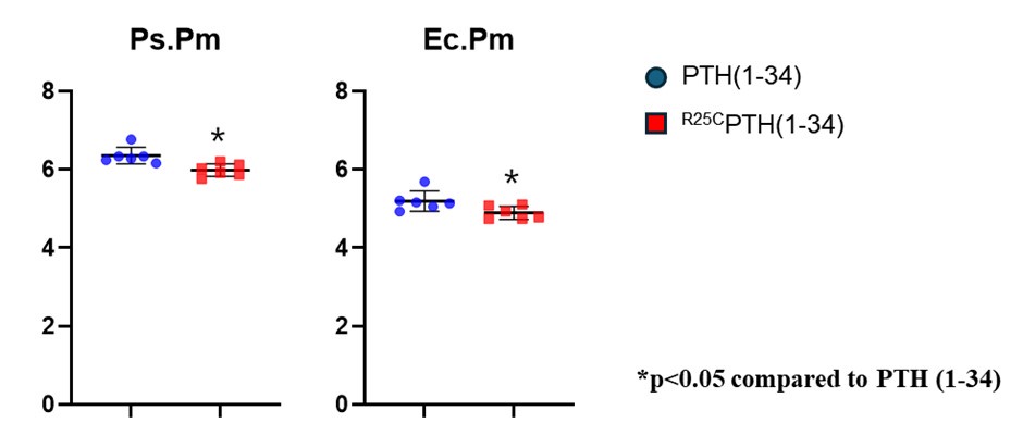
(4) It is also puzzling that both dimeric and monomeric PTH lead to a reduction in total bone area (cross sectional area?). This would suggest a reduction in bone growth. This should be discussed in the work.
In our experiment, the data showed an increase in cortical bone area in the PTH treatment group, but not in the PTH dimer treatment group. However, both dimeric and monomeric PTH treatments resulted in a reduction in total tissue area. We added revised sentence in page 13 line 317 and page 14 line 333 as follows:
“In addition, the data showed an increase in cortical bone area (Ct.Ar) in the PTH treatment group but not in the PTH dimer treatment group. However, both dimeric and monomeric PTH treatments reduced total tissue area (Tt.Ar), suggesting potential effects on bone growth in the width of mice or humans.”
“This study has several limitations. First, it is urgently necessary to determine whether dimeric <sup>R25C</sup>PTH is present in human patient serum. Second, TRAP staining showed an inhibitory effect of PTH treatment on the primary spongiosa area. However, the secondary spongiosa, which more accurately reflects bone remodeling (55), was not examined due to the barely detectable bone in this area in OVX-induced osteoporosis mouse models. Third, it is unclear whether similar bone phenotypes exist between human <sup>R25C</sup>PTH patients and dimeric <sup>R25C</sup>PTH-treated mice, particularly regarding low bone strength. Although the dimeric <sup>R25C</sup>PTH-treated group showed higher cortical BMD compared to WT-Sham or PTH groups, there was no difference in bone strength compared to the osteoporotic mouse model. Fourth, our study demonstrated that PTH or <sup>R25C</sup>PTH treatment decreased circumferential length, which could affect bone growth in width. However, whether this phenotype is also observed in patients treated with PTH or <sup>R25C</sup>PTH remains uncertain.”
Author Response
The following is the authors’ response to the original reviews.
We would like to thank the reviewers for their insightful comments and recommendations. We have extensively revised the manuscript in response to the valuable feedback. We believe the results is a more rigorous and thoughtful analysis of the data. Furthermore, our interpretation and discussion of the findings is more focused and highlights the importance of the circuit and its role in the response to stress. Thank you for helping to improve the presented science.
Key changes made in response to the reviewers comments include:
• Revision of statistical analyses for nearly all figures, with the addition of a new table of summary statistics to include F and/or t values alongside p-values.
• Addition of statistical analyses for all fiber photometry data.
• Examination of data for possible sex dependent effects.
• Clarification of breeding strategies and genotype differences, with added details to methods to improve clarity.
• Addressing concerns about the specificity of virus injections and the spread, with additional details added to methods.
• Modification of terminology related to goal-directed behavior based on reviewer feedback, including removal of the term from the manuscript.
• Clarification and additional data on the use of photostimulation and its effects, including efforts to inactivate neurons for further insight, despite technical challenges.
• Correction of grammatical errors throughout the manuscript.
Reviewer 1:
Despite the manuscript being generally well-written and easy to follow, there are several grammatical errors throughout that need to be addressed.
Thank you for highlighting this issue. Grammatical errors have been fixed in the revised version of the manuscript.
Only p values are given in the text to support statistical differences. This is not sufficient. F and/or t values should be given as well.
In response to this critique and similar comments from Reviewer 2, we re-evaluated our approach to statistical analyses and extensively revised analyses for nearly all figures. We also added a new table of summary statistics (Supplemental Table 1) containing the type of analysis, statistic, comparison, multiple comparisons, and p value(s). For Figures 4C-E, 5C, 6C-E, 7H-I, and 8H we analyzed these data using two-way repeated measures (RM) ANOVA that examined the main effect of time (either number of sessions or stimulation period) in the same animal and compared that to the main effect of genotype of the animal (Cre+ vs Cre-), and if there was an interaction. For Supplemental Figure 7A we also conducted a two-way RM ANOVA with time as a factor and activity state (number of port activations in active vs inactive nose port) as the other in Cre+ mice. For Figures 5D-E we conducted a two-way mixed model ANOVA that accounted and corrected for missing data. In figures that only compared two groups of data (Figures 5F-L, 6F, 8C-D, 8I, and Supp 6F-G) we used two-tailed t-test for the analysis. If our question and/or hypothesis required us to conduct multiple comparisons between or within treatments, we conducted Bonferroni’s multiple comparisons test for post hoc analysis (we note which groups we compared in Supplemental Table 1). For figures that did or did not show a change in calcium activity (Figure 3G, 3I-K, 7B, 7D-E, 8E-F), we compared waveform confidence intervals (Jean-Richard-Dit-Bressel, Clifford, McNally, 2020). The time windows we used as comparison are noted in Supplemental Table 1, and if the comparisons were significant at 95%, 99%, and 99.9% thresholds.
None of prior comparisons in prior analyses that were significant were found to have fallen below thresh holds for significance. Of those found to be not significantly different, only one change was noted. In Figure 6E there was now a significant baseline difference between Cre+ and Cre- mice with Cre- mice taking longer to first engage the port compared to Cre+ mice (p=0.045). Although the more rigorous approach the statistical analyses did not change our interpretations we feel the enhanced the paper and thank the reviewer for pushing this improvement.
Moreover, the fibre photometry data does not appear to have any statistical analyses reported - only confidence intervals represented in the figures without any mention of whether the null hypothesis that the elevations in activity observed are different from the baseline.
This is particularly important where there is ambiguity, such as in Figure 3K, where the spontaneous activity of the animal appears to correlate with a spike in activity but the text mentions that there is no such difference. Without statistics, this is difficult to judge.
Thank you for highlighting this critical point and providing an opportunity to strengthen our manuscript. We added statistical analyses of all fiber photometry data using a recently described approach based on waveform confidence intervals (Jean-Richard-Dit-Bressel, Clifford, McNally, 2020). In the statistical summary (Supplemental Table 1) we note the time window that we used for comparison in each analysis and if the comparisons were significant at 95%, 99%, and 99.9% thresholds. Thank you from highlighting this and helping make the manuscript stronger.
With respect to Figure 3K, we are not certain we understood the spike in activity the reviewer referred to. Figure 3J and K include both velocity data (gold) and Ca2+ dependent signal (blue). We used episodes of velocity that were comparable to the avoidance respond during the ambush test and no significant differences in the Ca2+ signal when gating around changes in velocity in the absence of stressor (Supplemental Table1). This is in contrast to the significant change in Ca2+ signal following a mock predator ambush (Figure 3J). We interpret these data together to indicate that locomotion does not correlate with an increase in calcium activity in SuMVGLUT2+::POA neurons, but that coping to a stressor does. This conclusion is further examined in supplemental Figure 5, including examining cross-correlation to test for temporally offset relationship between velocity and Ca2+ signal in SUMVGLUT2+::POA neurons.
The use of photostimulation only is unfortunate, it would have been really nice to see some inactivation of these neurons as well. This is because of the well-documented issues with being able to determine whether photostimulation is occurring in a physiological manner, and therefore makes certain data difficult to interpret. For instance, with regards to the 'active coping' behaviours - is this really the correct characterisation of what's going on? I wonder if the mice simply had developed immobile responding as a coping strategy but when they experience stimulation of these neurons that they find aversive, immobility is not sufficient to deal with the summative effects of the aversion from the swimming task as well as from the neuronal activation? An inactivation study would be more convincing.
We agree with the point of the reviewer, experiments demonstrating necessity of SUMVGLUT2+::POA neurons would have added to the story here. We carried out multiple experiments aimed at addressing questions about necessity of SuMVGLUT2+::POA neurons in stress coping behaviors, specifically the forced swim assay. Efforts included employing chemogenetic, optogenetic, and tetanus toxin-based methods. We observed no effects on locomotor activity or stress coping. These experiments are both technically difficult and challenging to interpret. Interpretation of negative results, as we obtained, is particularly difficult because of potential technical confounds. Selective targeting of SuMVGLUT2+::POA neurons for inhibition requires a process requiring three viral injections and two recombination steps, increasing variability and reducing the number of neurons impacted. Alternatively, photoinhibition targeting SuMVGLUT2+::POA cells can be done using Retro-AAV injected into POA and a fiber implant over SuM. We tried both approaches. Data obtained were difficult to interpret because of questions about adequate coverage of SuMVGLUT2+::POA population by virally expressed constructs and/or light spread arose. The challenge of adequate coverage to effectively prevent output from the targeted population is further confounded by challenges inherent in neural inhibition, specifically determining if the inhibition created at the cellular level is adequate to block output in the context of excitatory inputs or if neurons must be first engaged in a particular manner for inhibition to be effective. Baseline neural activity, release probability, and post-synaptic effects could all be relevant, which photo-inhibition will potentially not resolve. So, while the trend is to always show “necessary and sufficient” effects, we’ve tried nearly everything, and we simply cannot conclude much from our mixed results. There are also wellestablished problems with existing photo-inhibition methods, which while people use them and tout them, are often ignored. We have a lot of expertise in photo-inhibition optogenetics, and indeed have used it with some success, developed new methods, yet in this particular case we are unable to draw conclusions related to inhibition. People have experienced similar challenges in locus coeruleus neurons, which have very low basal activity, and inhibition with chemogenetics is very hard, as well as with optogenetic pump-based approaches, because the neurons fire robust rebound APs. We have spent almost 2.5 years trying to get this to work in this circuit because reviews have been insistent on this result for the paper to be conclusive. Unfortunately, it simply isn’t possible in our view until we know more about the cell types involved. This is all in spite of experience using the approach in many other publications.
We also employed less selective approaches, such as injecting AAV-DIO-tetanus toxin light chain (Tettox) constructs directly into SuM VGLUT2-Cre mice but found off target effects impacting animal wellbeing and impeding behavioral testing due viral spread to surrounding areas.
While we are disappointed for being unable to directly address questions about necessity of SuMVGLUT2+::POA neurons in active coping with experimental data, we were unable to obtain results allowing for clear interpretation across numerous other domains the reviewers requested. We also feel strongly that until we have a clear picture of the molecular cell type architecture in the SuM, and Cre-drivers to target subsets of neurons, this question will be difficult to resolve for any group. We are working now on RNAseq and related spatial transcriptomics efforts in the SuM and examining additional behavioral paradigm to resolve these issues, so stay tuned for future publications.
Accordingly, we avoid making statements relating to necessity in the manuscript. In spite of having several lines of physiological data with strong robust correlations behavior related to the SuMVGLUT2+::POA circuit.
Nose poke is only nominally instrumental as it cannot be shown to have a unique relationship with the outcome that is independent of the stimuli-outcome relationships (in the same way that a lever press can, for example). Moreover, there is nothing here to show that the behaviours are goal-directed.
Thank you for highlighting this point. Regarding goal-direct terminology, we removed this terminology from the manuscript. Since the mice perform highly selective (active vs inactive) port activation robustly across multiple days of training the behavior likely transitions to habitual behavior. We only tested the valuation of stimuli termination of the final day of training with time limited progressive ratio test. With respect to lever press versus active port activation, we are unclear how using a lever in this context would offer a different interpretation. Lever pressing may be more sensitive to changes in valuation when compared to nose poke port activation (Atalayer and Rowland 2008); however, in this study the focus of the operant behavior is separating innate behaviors for learned action–outcome instrumental learned behaviors for threat response (LeDoux and Daw 2018). The robust highly selective activation of the active port illustrated in Figure 6 fits as an action–outcome instrumental behavior wherein mice learn to engage the active but not inactive port to terminate photostimulation. The first activation of the port occurs through exploration of the arena but as demonstrated by the number of active port activations and the decline in time of the first active port engagement, mice expressing ChR2eYFP learn to engage the port to terminate the stimulation. To aid in illustrating this point we have added Supplemental Figure 7 showing active and inactive port activations for both Cre+ and Cre- mice. This adds clarity to high rate of selective port activation driven my stimulation of SUMVGLUT2+::POA neurons compared to controls. The elimination of goal directed and providing additional data narrows and supports one of the key points of the operant experiment.
With regards to Figure 1: This is a nice figure, but I wonder if some quantification of the pathways and their density might be helpful, perhaps by measuring the intensity of fluorescence in image J (as these are processes, not cell bodies that can be counted)? Mind you, they all look pretty dense so perhaps this is not necessary! However, because the authors are looking at projections in so-called 'stress-engaged regions', the amygdala seems conspicuous by its absence. Did the authors look in the amygdala and find no projections? If so it seems that this would be worth noting.
This is an interesting question but has proven to be a very technically challenging question. We consulted with several leaders who routinely use complimentary viral tracing methods in the field. We were unable to devise a method to provide a satisfactorily meaningful quantitative (as opposed to qualitative) approach to compare SUMVGLUT2+::POA to SuMVGLUT2+ projections. A few limitations are present that hinder a meaningful quantitative approach. One limitation was the need for different viral strategies to label the two populations. Labeling SuMVGLUT2+::POA neurons requires using VGLUT2-Flp mice with two injections into the POA and one into SuM. Two recombinase steps were required, reducing efficiency of overlap. This combination of viral injections, particularly the injections of RetroAAVs in the POA, can induce significant quantitative variability due to tropism, efficacy, and variability of retro-viral methods, and viral infection generally. These issues are often totally ignored in similar studies across the “neural circuit” landscape, but it doesn’t make them less relevant here.
Although people do this in the field, and show quantification, we actually believe that it can be a quite misleading read-out of functionally relevant circuitry, given that neurotransmitter release ultimately is amplified by receptors post-synaptically, and many examples of robust behavioral effects have been observed with low fiber tracing complimentary methods (McCall, Siuda et al. 2017). In contrast, the broader SuMVGLUT2+ population was labeled using a single injection into the SuM. This means there like more efficient expression of the fluorophore. Additionally, in areas that contain terminals and passing fibers understanding and interpreting fluorescent signal is challenging. Together, these factors limit a meaningful quantitative comparison and make an interpretation difficult to make. In this context, we focused on a conservative qualitative presentation to demonstrate two central points. That 1) SuMVGLUT2+::POA neurons are subset of SuMVGLUT2+ neurons that project to specific areas and that exclude dentate gyrus, and they 2) arborize extensively to multiple areas which have be linked to threat responses. We agree that there is much to be learned about how different populations in SuM connect to targets in different regions of the brain and to continue to examine this question with different techniques. A meaningful quantitative study comparing projections is technically complex and, we feel, beyond our ability for this study.
Also, for the reasons above we do not believe that quantification provides exceptional clarity with respect to the putative function of the circuit, glutamate released, or other cotransmitters given known amplification at the post-synaptic side of the circuit.
With regard to the amygdala, other studies on SuM projections have found efferent projections to amygdala (Ottersen, 1980; Vertes, 1992). In our study we were unable to definitively determine projections from SuMVGLUT2+::POA neurons to amygdala, which if present are not particularly dense. For this reason we were conservative and do not comment on this particular structure.
I would suggest removing the term goal-directed from the manuscript and just focusing on the active vs. passive distinction.
We removed the use of goal-directed. Thank you for helping us clarify our terminology.
The effect observed in Figure 7I is interesting, and I'm wondering if a rebound effect is the most likely explanation for this. Did the authors inhibit the VGAT neurons in this region at any other times and observe a similar rebound? If such a rebound was not observed it would suggest that it is something specific about this task that is producing the behaviour. I would like it if the authors could comment on this.
We agree that results showing the change in coping strategy (passive to active) in forced swim after but not during stimulation of SuMVGAT+ neurons is quite interesting (Figure 7I). This experiment activated SuMVGAT+ neurons during a section of the forced swim assay and mice showed a robust shift to mobility after the stimulation of SuMVGAT+ neurons stopped. We did not carry out inhibition of SuMVGAT+ neurons in this manuscript. As the reviewer suggested, strong inhibition of local SuM neurons, including SUMVGLUT2+::POA neurons, could lead to rebound activity that may shift coping behaviors in confusing ways. We agree this is an interesting idea but do not have data to support the hypothesis further at this time.
Reviewer 2
(1) These are very difficult, small brain regions to hit, and it is commendable to take on the circuit under investigation here. However, there is no evidence throughout the manuscript that the authors are reliably hitting the targets and the spread is comparable across experiments, groups, etc., decreasing the significance of the current findings. There are no hit/virus spread maps presented for any data, and the representative images are cropped to avoid showing the brain regions lateral and dorsal to the target regions. In images where you can see the adjacent regions, there appears expression of cell bodies (such as Supp 6B), suggesting a lack of SuM specificity to the injections.
We agree with the reviewer that the areas studied are small and technically challenging to hit. This was one of driving motivations for using multiple tools in tandem to restrict the area targeted for stimulation. Approaches included using a retrograde AAVs to express ChR2eFYP in SUMVGLUT2+::POA neurons; thereby, restricting expression to VGLUT2+ neurons that project to the POA. Targeting was further limited by placement of the optic fiber over cell bodies on SuM. Thus, only neurons that are VGLUT2+, project to the POA, and were close enough to the fiber were active by photostimulation. Regrettably, we were not able to compile images from mice where the fiber was misplaced leading to loss of behavioral effects. We would have liked to provide that here to address this comment. Unfortunately, generating heat maps for injections is not possible for anatomic studies that use unlabeled recombinase as part of an intersectional approach. Also determining the point of injection of a retroAAV can be difficult to accurately determine its location because neurons remote to injection site and their processes are labeled.
Experiments described in Supplemental Figure 6B on VGAT neurons in SuM were designed and interpreted to support the point that SUMVGLUT2+::POA neurons are a distinct population that does not overlap with GABAergic neurons. For this point it is important that we targeted SuM, but highly confined targeting is not needed to support the central interpretation of the data. We do see labeling in SuM in VGAT-Cre mice but photo stimulation of SuMVGAT+ neurons does not generate the behavioral changes seen with activation of SUMVGLUT2+::POA neurons. As the reviewer points out, SuM is small target and viral injection is likely to spread beyond the anatomic boundaries to other VGAT+ neurons in the region, which are not the focus here. The activation would be restricted by the spread of light from the fiber over SuM (estimated to be about a 200um sphere in all directions). We did not further examine projections or localization of VGAT+ neurons in this study but focused on the differential behavioral effects of SUMVGLUT2+::POA neurons.
(2) In addition, the whole brain tracing is very valuable, but there is very little quantification of the tracing. As the tracing is the first several figures and supp figure and the basis for the interpretation of the behavior results, it is important to understand things including how robust the POA projection is compared to the collateral regions, etc. Just a rep image for each of the first two figures is insufficient, especially given the above issue raised. The combination of validation of the restricted expression of viruses, rep images, and quantified tracing would add rigor that made the behavioral effects have more significance.
For example, in Fig 2, how can one be sure that the nature of the difference between the nonspecific anterograde glutamate neuron tracing and the Sum-POA glutamate neuron tracing is real when there is no quantification or validation of the hits and expression, nor any quantification showing the effects replicate across mice? It could be due to many factors, such as the spread up the tract of the injection in the nonspecific experiment resulting in the labeling of additional regions, etc.
Relatedly, in Supp 4, why isn’t C normalized to DAPI, which they show, or area? Similar for G what is the mcherry coverage/expression, and why isn’t Fos normalized to that?
Thank you for highlighting the importance of anatomy and the value of anatomy. Two points based on the anatomic studies are central to our interpretation of the experimental data. First, SUMVGLUT2+::POA are a distinct population within the SuM. We show this by demonstrating they are not GABAergic and that they do not project to dentate gyrus. Projections from SuM to dentate gyrus have been described in multiple studies (Boulland et al., 2009; Haglund et al., 1987; Hashimotodani et al., 2018; Vertes, 1992) and we demonstrate them here for SuMVGLUT2+ cells. Using an intersectional approach in VGLUT2-Flp mice we show SUMVGLUT2+::POA neurons do not project to dentate gyrus. We show cell bodies of SUMVGLUT2+::POA neurons located in SuM across multiple figures including clear brain images. Thus, SUMVGLUT2+::POA neurons are SuM neurons that do not project to dentate gyrus, are not GABAergic, send projections to a distinct subset of targets, most notably excluding dentate gyrus. Second, SUMVGLUT2+::POA neurons arborize sending projections to multiple regions. We show this using a combinatorial genetic and viral approach to restrict expression of eYFP to only neurons that are in SuM (based on viral injection), project to the POA (based on retrograde AAV injection in POA), and VGLUT2+ (VGLUT2-Flp mice). Thus, any eYFP labeled projection comes from SUMVGLUT2+::POA neurons. We further confirmed projections using retroAAV injection into areas identified using anterograde approaches (Supplemental Figure 2). As discussed above in replies to Reviewer 1, we feel limitations are present that preclude meaningful quantitative analysis. We thus opted for a conservative interpretation as outlined.
Prior studies have shown efferent projections from SuM to many areas, and projections to dentate gyrus have received substantial attention (Bouland et al., 2009; Haglund, Swanson, and Kohler, 1984; Hashimotodani et al., 2018; Soussi et al., 2010; Vertes, 1992; Pan and McNaugton, 2004). We saw many of the same projections from SuMVGLUT2+ neurons. We found no projections from SUMVGLUT2+::POA neurons to dentate gyrus (Figure 2). Our description of SuM projection to dentate gyrus is not new but finding a population of neurons in SuM that does not project to dentate gyrus but does project to other regions in hippocampus is new. This finding cannot be explained by spread of the virus in the tract or non-selective labeling.
(3) The authors state that they use male and female mice, but they do not describe the n’s for each experiment or address sex as a biological variable in the design here. As there are baseline sex differences in locomotion, stress responses, etc., these could easily factor into behavioral effects observed here.
Sex specific effects are possible; however, the studies presented here were not designed or powered to directly examine them. A point about experimental design that helps mitigate against strong sex dependent effect is that often the paradigm we used examined baseline (pre-stimulation) behavior, how behavior changed during stimulation, and how behavior returned (or not) to baseline after stimulation. Thus, we test changes in individual behaviors. Although we had limited statistical power, we conducted analyses to examine the effects of sex as variable in the experiments and found no differences among males and females.
(4) In a similar vein as the above, the authors appear to use mice of different genotypes (however the exact genotypes and breeding strategy are not described) for their circuit manipulation studies without first validating that baseline behavioral expression, habituation, stress responses are not different. Therefore, it is unclear how to interpret the behavioral effects of circuit manipulation. For example in 7H, what would the VGLUT2-Cre mouse with control virus look like over time? Time is a confound for these behaviors, as mice often habituate to the task, and this varies from genotype to genotype. In Fig 8H, it looks like there may be some baseline differences between genotypes- what is normal food consumption like in these mice compared to each other? Do Cre+ mice just locomote and/or eat less? This issue exists across the figures and is related to issues of statistics, potential genotype differences, and other experimental design issues as described, as well as the question about the possibility of a general locomotor difference (vs only stress-induced). In addition, the authors use a control virus for the control groups in VGAT-Cre manipulation studies but do not explain the reasoning for the difference in approach.
Thank you for highlighting the need for greater clarity about the breeding strategies used and for these related questions. We address the breeding strategy and then move to address the additional concerns raised. We have added details to the methods section to address this point. For VGLUT2-Cre mice we use litter mates controls from Cre/WT x WT/WT cross. The VGLUT2-Cre line (RRID:IMSR_JAX:028863) (Vong L , et al. 2011) used here been used in many other reports. We are not aware of any reports indicating a phenotype associated with the addition of the IRES-Cre to the Slc17a6 loci and there is no expected impact of expression of VGLUT2. Also, we see in many of the experiments here that the baseline (Figures 4, 5, and 7) behaviors are not different between the Cre+ and Cre- mice. For VGAT-Cre mice we used a different breeding strategy that allowed us to achieve greater control of the composition of litters and more efficient cohorts cohort. A Cre/Cre x WT/WT cross yielded all Cre/WT litters. The AAV injected, ChR2eYFP or eYFP, allowed us to balance the cohort.
Regarding Figure 7H, which shows time immobile on the second day of a swim test, data from the Cre- mice demonstrate the natural course of progression during the second day of the test. The control mice in the VGAT-Cre cohort (Figure 7I) have similar trend. The change in behavior during the stimulation period in the Cre+ mice is caused by the activation of SUMVGLUT2+::POA neurons. The behavioral shift largely, but not completely, returns to baseline when the photostimulation stops. We have no reason to believe a VGLUT2-Cre+ mouse injected with control AAV to express eYFP would be different from WT littermate injected with AVV expressing ChR2eYFP in a Cre dependent manner.
Turning to concerns related to 8H, which shows data from fasted mice quantify time spent interacting with food pellet immediately after presentation of a chow pellet, we found no significant difference between the control and Cre+ mice. We unaware of any evidence indicating that the two groups should have a different baseline since the Cre insertion is not expected to alter gene expression and we are unaware of reports of a phenotype relating to feeding and the presence of the transgene in this mouse line. Even if there were a small baseline shift this would not explain the large abrupt shift induced by the photostimulation. As noted above, we saw shifts in behavior abruptly induced by the initiation of photostimulation when compared to baseline in multiple experiments. This shift would not be explained by a hypothetical difference in the baseline behaviors of litter mates.
(5) The statistics used throughout are inappropriate. The authors use serial Mann-Whitney U tests without a description of data distributions within and across groups. Further, they do not use any overall F tests even though most of the data are presented with more than two bars on the same graph. Stats should be employed according to how the data are presented together on a graph. For example, stats for pre-stim, stim, and post-stim behavior X between Cre+ and Cre- groups should employ something like a two-way repeated measures ANOVA, with post-hoc comparisons following up on those effects and interactions. There are many instances in which one group changes over time or there could be overall main effects of genotype. Not only is serially using Mann-Whitney tests within the same panel misleading and statistically inaccurate, but it cherry-picks the comparisons to be made to avoid more complex results. It is difficult to comprehend the effects of the manipulations presented without more careful consideration of the appropriate options for statistical analysis.
We thank the reviewer for pointing this out and suggesting alterative analyses, we agree with the assessment on this topic. Therefore, we have extensively revised the statical approach to our data using the suggested approach. Reviewer 1 also made a similar comment, and we would like to point to our reply to reviewer 1’s second point in regard to what we changed and added to the new statistical analyses. Further, we have added a full table detailing the statical values for each figure to the paper.
Conceptual:
(6) What does the signal look like at the terminals in the POA? Any suggestion from the data that the projection to the POA is important?
This is an interesting question that we will pursue in future investigations into the roles of the POA. We used the projection to the POA from SuM to identify a subpopulation in SuM and we were surprised to find the extensive arborization of these neurons to many areas associated with threat responses. We focused on the cell bodies as “hubs” with many “spokes”. Extensive studies are needed to understand the roles of individual projections and their targets. There is also the hypothetical technical challenge of manipulating one projection without activating retrograde propagation of action potentials to the soma. At the current time we have no specific insights into the roles of the isolated projection to POA. Interpretation of experiments activating only “spoke” of the hub would be challenging. Simple terminal stimulation experiments are challenged by the need to separate POA projections from activation of passing fibers targeting more anterior structures of the accumbens and septum.
(7) Is this distinguishing active coping behavior without a locomotor phenotype? For example, Fig. 5I and other figure panels show a distance effect of stimulation (but see issues raised about the genotype of comparison groups). In addition, locomotor behavior is not included for many behaviors, so it is hard to completely buy the interpretation presented.
We agree with the reviewer and thank them for highlighting this fundamental challenge in studies examining active coping behaviors in rodents, which requires movement. Additionally, actively responding to threatening stressors would include increased locomotor activity. Separation of movement alone from active coping can be challenging. Because of these concerns we undertook experiments using diverse behavioral paradigms to examine the elicited behaviors and the recruitment of SuMVGLUT2+::POA neurons to stressors. We conducted experiments to directly examine behaviors evoked by photoactivation of SuMVGLUT2+::POA. In these experiments we observed a diversity of behaviors including increased locomotion and jumping but also treading/digging (Figure 4). These are behaviors elicited in mice by threatening and noxious stimuli. An Increase of running or only jumping could signify a specific locomotor effect, but this is not what was observed. Based on these behaviors, we expected to find evidence of increase movement in open field (Figure 5G-I) and light dark choice (Figure 5J-L) assays. For many of the assays, reporting distance traveled is not practical. An important set of experiments that argues against a generic increase in locomotion is the operant behavior experiments, which require the animal to engage in a learned behavior while receiving photostimulation of SuMVGLUT2+::POA neurons (Figure 6). This is particularly true for testing using a progressive ratio when the time of ongoing photostimulation is longer, yet animals actively and selectively engage the active port (Figure 6G-H). Further, we saw a shift in behavioral strategy induce by photoactivation in forced swim test (Figure 7H). Thus, activation of SUMVGLUT2+::POA neurons elicited a range of behaviors that included swimming, jumping, treading, and learned response, not just increased movement. Together these data strongly argue that SuMVGLUT2+::POA neurons do not only promote increased locomotor behavior. We interpret these data together with the data from fiber photometry studies to show SuMVGLUT2+::POA neurons are recruited during acute stressors, contribute to aversive affective component of stress, and promote active behaviors without constraining the behavioral pattern.
Regarding genotype, we address this in comments above as well but believe that clarifying the use of litter mates, the extensive use of the VGLUT2-Cre line by multiple groups, and experimental design allowing for comparison to baseline, stimulation evoked, and post stimulation behaviors within and across genotypes mitigate possible concerns relating to the genotype.
(8) What is the role of GABA neurons in the SuM and how does this relate to their function and interaction with glutamate neurons? In Supp 8, GABA neuron activation also modulates locomotion and in Fig 7 there is an effect on immobility, so this seems pretty important for the overall interpretation and should probably be mentioned in the abstract.
Thank you for noting these interesting findings. We added text to highlight these findings to the abstract. Possible roles of GABAergic neurons in SuM extend beyond the scope of the current study particularly since SuM neurons have been shown to release both GABA and glutamate (Li Y, Bao H, Luo Y, et al. 2020, Root DH, Zhang S, Barker DJ et al. 2018). GABAergic neurons regulate dentate gyrus (Ajibola MI, Wu JW, Abdulmajeed WI, Lien CC 2021), REM sleep (Billwiller F, Renouard L, Clement O, Fort P, Luppi PH 2017), and novelty processing Chen S, He L, Huang AJY, Boehringer R et al. 2020). The population of exclusively GABAergic vs dual neurotransmitter neurons in SuM requires further dissection to be understood. How they may relate to SUMVGLUT2+::POA neurons require further investigation.
Questions about figure presentation:
(9) In Fig 3, why are heat maps shown as a single animal for the first couple and a group average for the others?
Thank you for highlighting this point for further clarification. We modified the labels in the figure to help make clear which figures are from one animal across multiple trials and those that are from multiple animals. In the ambush assay each animal one had one trial, to avoid habituation to the mock predator. Accordingly, we do not have multiple trials for each animal in this test. In contrast, the dunk assay (10 trial/animal) and the shock (5 trials/animal) had multiple trials for each animal. We present data from a representative animal when there are multiple trials per animal and the aggerate data.
Why is the temporal resolution for J and K different even though the time scale shown is the same?
Thank you for noticing this error carried forward from a prior draft of the figure so we could correct it. We replaced the image in 3J with a more correctly scaled heatmap.
What is the evidence that these signal changes are not due to movement per se?
Thank you for the question. There are two points of evidence. First, all the 465 nm excitation (Ca2+ dependent) data was collected in interleaved fashion with 415 nm (isosbestic) excitation data. The isosbestic signal is derived from GCaMP emission but is independent of Ca2+ binding (Martianova E, Aronson S, Proulx CD. 2019). This approach, time-division multiplexing, can correct calcium-dependent for changes in signal most often due to mechanical change. The second piece of evidence is experimental. Using multiple cohorts of mice, we examined if the change in Ca2+ signal was correlated with movement. We used the threshold of velocity of movement seen following the ambush. We found no correlation between high velocity movements and Ca2+ signal (Figure 3K) including cross correlational analysis (Supplemental figure 5). Based on these points together we conclude the change in the Ca2+ signal in SUMVGLUT2+::POA neurons is not due to movement induced mechanical changes and we find no correlation to movement unless a stressor is present, i.e. mock predator ambush or forced swim. Further, the stressors evoke very different locomotor responses fleeing, jumping, or swimming.
(10) In Fig 4, the authors carefully code various behaviors in mice. While they pick a few and show them as bars, they do not show the distribution of behaviors in Cre- vs Cre+ mice before manipulation (to show they have similar behaviors) or how these behaviors shift categories in each group with stimulation. Which behaviors in each group are shifting to others across the stim and post-stim periods compared to pre-stim?
This is an important point. We selected behaviors to highlight in Figure4 C-E because these behaviors are exhibited in response to stress (De Boer & Koolhaas, 2003; van Erp et al., 1994). For the highlighted behaviors, jumping, treading/digging, grooming, we show baseline (pre photostimulation), stimulation, and post stimulation for Cre+ and Cre- mice with the values for each animal plotted. We show all nine behaviors as a heat map in Figure 4B. The panels show changes that may occur as a function of time and show changes induced by photostimulation.
The heatmaps demonstrate that photostimulation of SUMVGLUT2+::POA neurons causes a suppression of walking, grooming, and immobile behaviors with an increase in jumping, digging/treading, and rapid locomotion. After stimulation stops, there is an increase in grooming and time immobile. The control mice show a range of behaviors with no shifts noted with the onset or termination of photostimulation.
Of note, issues of statistics, genotype, and SABV are important here. For example, the hint that treading/digging may have a slightly different pre-stim basal expression, it seems important to first evaluate strain and sex differences before interpreting these data.
We examined the effects of sex as a biological variable in the experiments reported in the manuscript and found no differences among males and females in any of the experiments where we had enough animals in each sex (minimum of 5 mice) for meaningful comparisons. We did this by comparing means and SEM of males and females within each group (e.g. Cre+ males vs Cre+ female, Cre- males vs Cre- females) and then conducted a t-test to see if there was a difference. For figures that show time as a variable (e.g Figure 6C-E), we compared males and females with time x sex as main factors and compared them (including multiple comparisons if needed). We found no significant main effects or interactions between males and females. Because of this, and to maximize statistical power, we decided to move forward to keep males and females together in all the analyses presented in the manuscript. It is worth noting also that the core of the experimental design employed is a change in behavior caused by photostimulation. The mice are also the same strain with only difference being the modification to add an IRES and sequence for Cre behind the coding sequence of the Slc17A6 (VGLUT2) gene.
(11) Why do the authors use 10 Hz stimulation primarily? is this a physiologically relevant stim frequency? They show that they get effects with 1 Hz, which can be quite different in terms of plasticity compared to 10 Hz.
Thank you for the raising this important question. Because tests like open field and forced swim are subject to habituation and cannot be run multiple times per animal a test frequency was needed to use across multiple experiments for consistency. The frequency of 10Hz was selected because it falls within the rate of reported firing rates for SuM neurons (Farrel et al., 2021; Pedersen et al., 2017) and based on the robust but sub maximal effects seen in the real-time place preference assays. Identification of the native firing rates during stress response would be ideal but gathering this data for the identified population remains a dauting task.
(12) In Fig 5A-F, it is unclear whether locomotion differences are playing a role. Entrances (which are low for both groups) are shown but distance traveled or velocity are not.
In B, there is no color in the lower left panel. where are these mice spending their time? How is the entirety of the upper left panel brighter than the lower left? If the heat map is based on time distribution during the session, there should be more color in between blue and red in the lower left when you start to lose the red hot spots in the upper left, for example. That is, the mice have to be somewhere in apparatus. If the heat map is based on distance, it would seem the Cre- mice move less during the stim.
We appreciate the opportunity to address this question, and the attention to detail the reviewer applied to our paper. In the real time place preference test (RTPP) stimulation would only be provided while the animal was on the stimulation side. Mice quickly leave the stimulation side of the arena, as seen in the supplemental video, particularly at the higher frequencies. Thus, the time stimulation is applied is quite low. The mice often retreat to a corner from entering the stimulation side during trials using higher frequency stimulation. Changing locomotor activity along could drive changes in the number entrances but we did not find this. In regard to the heat map, the color scale is dynamically set for each of the paired examples that are pulled from a single trial. To maximize the visibility between the paired examples the color scale does not transfer between the trials. As a result, in the example for 10 Hz the mouse spent a larger amount of time in the in the area corresponding to the lower right corner of the image and the maximum value of the color scale is assigned to that region. As seen in the supplemental video, mice often retreated to the corner of the non-stimulation side after entering the stimulation side. The control animal did not spend a concentrated amount of time in any one region, thus there is a lack of warmer colors. In contrast the baseline condition both Cre+ and Cre- mice spent time in areas disturbed on both sides of arena, as expected. As a result, the maximum value in the heat map is lower and more area are coded in warmer colors allowing for easier visual comparison between the pair. Using the scale for the 10 Hz pair across all leads to mostly dark images. We considered ways to optimized visualization across and within pairs and focused on the within pair comparison for visualization.
(13) By starting with 1 hz, are the experimenters inducing LTD in the circuit? what would happen if you stop stimming after the first epoch? Would the behavioral effect continue? What does the heat map for the 1 hz stim look like?
Relatedly, it is a lot of consistent stimulation over time and you likely would get glutamate depletion without a break in the stim for that long.
Thank you for the opportunity to add clarity around this point regarding the trials in RTPP testing. Importantly, the trials were not carried out in order of increasing frequency of stimulation, as plotted. Rather, the order of trials was, to the extent possible with the number of mice, counterbalanced across the five conditions. Thus, possible contribution of effects of one trial on the next were minimized by altering the order of the trials.
We have added a heat map for the 1 Hz condition to figure 5B.
For experiments on RTPP the average stimulation time at 10Hz was less than 10 seconds per event. As a result, the data are unlikely to be affected by possible depletion of synaptic glutamate. For experiments using sustained stimulation (open field or light dark choice assays) we have no clear data to address if this might be a factor where 10Hz stimulation was applied for the entire trial.
(14) In Fig 6, the authors show that the Cre- mice just don't do the task, so it is unclear what the utility of the rest of the figure is (such as the PR part). Relatedly, the pause is dependent on the activation, so isn't C just the same as D? In G and H, why ids a subset of Cre+ mice shown?
Why not all mice, including Cre- mice?
Thank you for the opportunity to improve the clarity of this section. A central aspect of the experiments in Figure 6 is the aversiveness of SUMVGLUT2+::POA neuron photostimulation, as shown in Figure 5B-F. The aversion to photostimulation drives task performance in the negative reinforcer paradigm. The mice perform a task (active port activation) to terminate the negative reinforcer (photostimulation of SuMVGLUT2+::POA neurons). Accordingly, control mice are not expected to perform the task because SuMVGLUT2+::POA neurons are not activated and, thus the mice are not motivated to perform the task.
A central point we aim to covey in this figure is that while SuMVGLUT2+::POA neurons are being stimulated, mice perform the operant task. They selectively activated the active port (Supplemental Figure 7). As expected, control mice activate the active port at a low level in the process of exploring the arena. This diminishes on subsequent trials as mice habituate to the arena (Figure 6D). The data in Figures 6 C and D are related but can be divergent. Each pause in stimulation requires a port activation of a FR1 test but the number of port activations can exceed the pauses, which are 10 seconds long, if the animal continues to activate the port. Comparing data in Figures 6 C and D revels that mice generally activated the port two to three times for each pause earned with a trend towards greater efficiency on day 4 with more rewards and fewer activations.
The purpose of the progressive ratio test is to examine if photostimulation of SuMVGLUT2+::POA continues to drive behavior as the effort required to terminate the negative stimuli increases. As seen in Figures 6 G and H, the stimulation of SuMVGLUT2+::POA neurons remains highly motivating. In the 20-minute trial we did not find a break point even as the number of port activations required to pause the stimulation exceed 50. We do not show the Cre- mice is Figure 6G and H because they did not perform the task, as seen in Figure 6F. For technical reasons in early trials, we have fully timely time stamped data for rewards and port activations from a subset of the Cre+ mice. Of note, this contains both the highest and lowest performing mice from the entire data set.
Taken together, we interpret the results of the operant behavioral testing as demonstrating that SuMVGLUT2+::POA neuron activation is aversive, can drive performance of an operant tasks (as opposed to fixed escape behaviors), and is highly motivating.
(15) In Fig 7, what does the GCaMP signal look like if aligned to the onset of immobility? It looks like since the hindpaw swimming is short and seems to precede immobility, and the increase in the signal is ramping up at the onset of hindpaw swimming, it may be that the calcium signal is aligned with the onset of immobility.
What does it look like for swimming onset?
In I, what is the temporal resolution for the decrease in immobility? Does it start prior to the termination of the stim, or does it require some elapsed time after the termination, etc?
Thank for the opportunity to addresses these points and improve that clarity of our interpretation of the data. Regarding aligning the Ca2+ signal from fiber photometry recordings to swimming onset and offset, it is important to note that the swimming bouts are not the same length. As a result, in the time prior to alignment to offset of behaviors animals will have been swimming for different lengths of time. In Figure 7 C, we use the behavioral heat map to convey the behavioral average. Below we show the Ca2+ dependent signal aligned at the offset of hindpaw swim for an individual mouse (A) and for the total cohort (B). This alignment shows that the Ca2+ dependent signal declines corresponding to the termination of hindpaw swimming. Because these bouts last less than the total the widow shown, the data is largely included in Figure 7 C and D, which is aligned to onset. Due to the nuance of the difference is the alignment and the partial redundancy, we elected to include the requested alignment to swimming offset in the reply rather in primary figure.
Author response image 1.
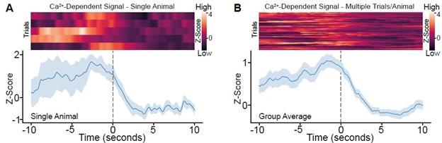
Turning to the question regarding swimming onset, the animals started swimming immediately when placed in the water and maintained swimming and climbing behaviors until shifting behaviors as illustrated in Figure 7A and B. During this time the Ca2+-dependent signal was elevated but there is only one trial per animal. This question can perhaps be better addressed in the dunk assay presented in Figure 3C, F and G and Supplemental Figure 4 H and I. Here swimming started with each dunk and the Ca2+ signal increased.
Regarding the question for about figure 7I. We scored for entire periods (2 mins) in aggerate. We noted in videos of the behavior test that there was an abrupt decrease in immobility tightly corresponding to the end of stimulation. In a few animals this shift occurred approximately 15-20s before the end of stimulation. This may relate to the depletion of neurotransmitter as suggested by the reviewer.
Reviewer 3
Major points
(1) Results in Figure 1 suggested that SuM-Vglu2::POA projected not only POA but also to the diverse brain regions. We can think of two models which account for this. One is that homogeneous populations of neurons in SuM-Vglu2::POA have collaterals and innervated all the efferent targets shown in Figure 1. Another is to think of distinct subpopulations of neurons projecting subsets of efferent targets shown in Figure 1 as well as POA. It is suggested to address this by combining approaches taken in experiments for Figure 1 and Supplemental Figure 2.
Thank you for raising this interesting point. We have attempted combining retroAAV injections into multiple areas that receive projections from SUMVGLUT2+::POA neurons. However, we have found the results unsatisfactory for separating the two models proposed. Using eYFP and tdTomato expressing we saw some overlapping expressing in SuM. We are not able to conclude if this indicates separate populations or partial labeling of a homogenous populations. A third option seems possible as well. There could be a mix of neurons projecting to different combinations of downstream targets. This seems particularly difficult to address using fluorophores. We are preparing to apply additional methodologies to this question, but it extends beyond the scope of this manuscript.
(2) Since the authors drew a hypothetical model in which the diverse brain regions mediate the effect of SuM-Vglu2::POA activation in behavioral alterations at least in part, examination of the concurrent activation of those brain regions upon photoactivation of SuM-Vglu2::POA. This must help the readers to understand which neural circuits act upon the induction of active coping behavior under stress.
Thank you for raising this important point. We agree that activating glutamatergic neurons should lead to activation of post synaptic neurons in the target regions. Delineating this in vivo is less straight forward. Doing so requires much greater knowledge of post synaptic partners of SUMVGLUT2+::POA neurons. There are a number of issues that would need to be accounted for. Undertaking two color photo stimulation plus fiber photometry is possible but not a technical triviality. Further, it is possible that we would measure Ca2+ signals in neurons that have no relevant input or that local circuits in a region may shape the signal. We would also lack temporal resolution to identify mono-postsynaptic vs polysynaptic connections. Thus, we would struggle to know if the change in signal was due to the excitatory input from SuM or from a second region. At present, we remain unclear on how to pursue this question experimentally in a manner that is likely to generate clearly interpretable results.
(3) In Figure 4, "active coping behaviors" must be called "behaviors relevant to the active behaviors" or "active coping-like behaviors", since those behaviors were in the absence of stressors to cope with.
Thank you for the suggestion on how to clarify our terminology. We have adopted the active coping-like term.
(4) For the Dunk test, it is suggested to describe the results and methods more in detail, since the readers would be new to it. In particular, the mice could change their behavior between dunks under this test, although they still showed immobility across trials as in Supplemental Figure 4I. Since neural activity during the test was summarized across trials as in Figure 3, it is critical to examine whether the behavior changes according to time.
Thank you for identifying this opportunity to improve our manuscript. We have expanded and added a detailed description of the dunk test in the methods section.
As for Supplemental Figure 4I, we apologize for the confusion because the purpose of this figure is to show that mice remained mobile for the entire 30-second dunk trial. This did not appreciably change over the 10 trials. We have revised this figure to plot both immobile and mobile time to achieve greater clarity on this point.
Minor points
Typos
In Figure 1, please add a serotype of AAVs to make it compatible with other figures and their legends.
In the main text and Figure 2K, the authors used MHb/LHb and mHb/lHb in a mixed fashion. Please make them unified.
In the figure legend of Figure 6, change "SuMVGLUT2+::POA neurons drive" to "SuMVGLUT2+::POA neurons " in the title.
In line 86, please change "Retro-AAV2-Nuc-flox(mCherry)-eGFP" to "AAV5-Nuc-flox(mCherry)eGFP".
In line 80, please change "Positive controls" to "As positive controls, ".
Thank you for taking the time and making the effort to identify and call these out. We have corrected them.
Author Response
The following is the authors’ response to the previous reviews
The revised manuscript is much improved - many unclear points are now better explained. However, in our opinion, some issues could still be significantly improved.
- Statistics: none of us are experts in statistics but several things remain questionable in our opinion and if it were our study, we would consult with an expert:
a) while we understand the authors note about N-chasing and p-hacking, we wonder how the number of N's was premeditated before obtaining the results. Why in 4M an N of 3 is sufficient while in 3E the N is >20 (and not mentioned). At the very least, we think it would be wise to be cautious when stating something as not-significant when it is clear (as in 4M) that the likelihood of it actually being statistically significant is quite large.
b) In most analyses, the data is not only normalized by actin or some other measure but also to the first (i.e left side on the graph) condition, resulting in identical data points that equal '1' (in Figure 4 alone - C; I; K; M; and O) - while this might be scientifically sound, it should be mentioned (the specific normalization) and also note that this technique shadows any real variance that exists in the original data in this condition. consider exploring techniques to overcome this issue.
c) In 3C, - if we understand the experiment, you want to convince us that the DIFFERENCE between eB2-FC compared to FC is larger in the control compared to the experiment. We are not absolutely sure that the statistical tools employed here are sufficient - which is why we would consult an expert.
A) We are aware that many studies do not consistently quantify such experiments. For example, there are essentially no published examples of the signalling timelines of EphB2 receptors as in Fig. 5. By striving to quantifying such biochemical effects, an unquantified experiment stands out, and so perhaps we were too strict by trying to quantify as many experiments as possible, resulting in low n’s for some of them. We acknowledge that additional experiments on EPHB1 protein stability may reach significance. We have adjusted our text on line 332-335 to point to this interesting trend, and slightly changed the conclusion to this section. Similarly, we commented on similar trends when describing Figs. 1E and 4G on lines 901 and 952.
B) For the Western blot band intensity normalisation, we believe that our method is scientifically sound. Normally, when the replicate samples are loaded on one gel and blotted on the same membrane, the experimenter only needs to normalise the target band intensity to its cognate loading control band intensity for quantitation. However, we usually have a large number of samples from multiple experiments, carried out on different dates. For example, in Fig. 4B,C there are 7 biological replicates collected from 7 experiments and in Fig. 4D there are 10 protein samples. It is not possible for us to run all samples on the same gel. In addition, due to the combined effects of variance in transfer efficiency, the potency of antibodies, detection efficiency and the developing time for each blot, it is practically impossible to generate similar band intensity for each batch. Thus, we use normalisation of test bands to the loading control for individual experiments, and this analysis method is widely accepted by reputable journals with a focus on biochemical experiments (for example: PMID 37695914: Fig. 3 A,B,C; PMID 36282215: Fig. 3 B,C,D,E; PMID 33843588: Fig. 3 C,D,E,F,G,H). Since the value of the first sample on the plot is 1, which is a hypothetical value and does not meet the parametric test requirement, we performed one-sample t-test for statistics when other samples are compared with the first sample (PMID 35243233 Fig. 6 A,B,C,D; https://www.graphpad.com/quickcalcs/oneSampleT1/, “A one sample t-test compares the mean with a hypothetical value. In most cases, the hypothetical value comes from theory. For example, if you express your data as 'percent of control', you can test whether the average differs significantly from 100.”). Thus, we believe that our normalisation and statistical methods are both correct with a large number of precedents.
C) This comment refers to the cell collapse experiment shown in Fig. 3C for which the data are plotted in Fig. 3D. We stand by the statistical method used. There are two groups of cells (CTRLCRISPR and MYCBP2 CRISPR) and two treatments for each cell group (Fc control and eB2), thus we should use two-way ANOVA. Since we compared the cell retraction effects of Fc and eB2 on the two groups of cells, Sidak post hoc comparison is the right method to avoid errors introduced by multiple comparisons. Here is an example of an eLife article that used the same statistical method for similar comparisons: PMID 37830910, Fig. 1 H,I. To make the comparison easier, we grouped the experiments by cell type (CTRLCRISPR and MYCBP2 CRISPR) as opposed to by treatment. Below, the old version is on the right, and the new version is on the left. The conclusion is that eB2 induces less cell collapse in cells depleted of MYCBP2, when compared to the control cells. However, eB2 is still able to collapse cells lacking MYCBP2.
Author response image 1.
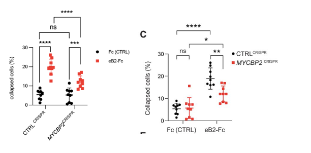
Revisiting these data, we noticed an error introduced when CC compiled the data used to generate Fig. 3D. The data were acquired from nine biological replicates per condition. CC used a mix of two methods for cell collapse rate calculation: the first method involved the sum of collapsed cells and all cells from multiple regions of one coverslip (biological replicate). The second method involved computing a collapse rate in each region which then was used to calculate the average collapse rate for the entire coverslip (technical replicate). Given the small cell numbers due to sparse culture conditions, we believe that the first method is a more conservative approach. We hence re-plotted all replicate data using the first method. This resulted in slightly different % collapse and p values. These were changed accordingly in the text and plot and do not affect the conclusion of this experiment.
2) thanks for the clarification that the interaction between the extracellular domain of EPHB2 and MYCBP2 might not occur directly - however, unless we missed this it was not clearly stated in the text. It is an important point and also a cool direction for the future - to find the elusive co-receptor that actually helps EPHB2 and MYCBP2 form a complex.
We now also refer to this in the results section on line 215.
“Since EPHB2 is a transmembrane protein and MYCBP2 is localised in the cytosol, these experiments suggest that the interaction between the extracellular domain of EPHB2 and MYCBP2 might be indirect and mediated by other unknown transmembrane proteins.”
3) The Hela CRISPR cell line is better explained in the response letter but still not sufficiently explained in the text for a non-expert reader. If the authors want any reader to comprehend this, we would strongly recommend adding a scheme.
We now include a schematic outlining the CRISPR cell generation as Fig. 3A and its description on line 926.
Author response image 2.
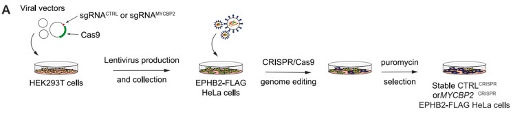
4) To clarify some of our previous (and persisting) concerns about Figure 3D/E - it is true that a reduction in 25% of cell size is dramatic. But (if we understand correctly) your claim is that a reduction in 22% (this is a guess, as the actual numbers are not supplies) is significantly less than 25%. Even if it is, statistically speaking, significant, what is the physiological relevance of this very slight effect? In this experiment, the N was quite large, and we wonder if the images in D are representative - it would be nice to label the data points in E to highlight which images you used.
We now mention the average cell area contraction measurements in the legend to Fig. 3F on line 935. We also tracked down the individual cells shown in Fig. 3E and they are now labelled as data points in blue in Fig. 3F. HeLa cell collapse is a simplified model of EPHB2 function and we do not know whether the difference between the behaviour of CTRLCRISPR and MYCBP2 CRISPR cells is physiologically significant and thus we prefer not to speculate on this.
5) Figure 3F and other stripe assays - In the end, it is your choice how to quantify. We believe that quantifying area of overlap is a more informative and objective measurement that might actually benefit your analyses. That said, if you do keep the quantification as it is now, you have to define the threshold of what you mean by "cell/s (or an axon in 7A, where it is even more complicated as are you eluding to primary, secondary, or even smaller branches) are RESIDING within the stripe". Is 1% overlap sufficient or do you need 10 or 50% overlap?
We now added this statement to the methods on line 745: “A cell was considered to be on an ephrin-B2 stripe when more than 50% of its nucleus was located on that stripe”. For chick explant stripe assay, when measuring the length of an axon on a stripe, we only measured the main axons originated from the explants.
For explant/stripe experiments in Fig. 7 AB, we now use the term “GFP-expressing neurite” rather than “branch”. This was already present in the results of the previous version, but the methods and legend needed to be brought up to date (lines 786 and 1008. We think that “branch” was a confusing term that was supposed to mean the same thing as “neurite” but came across as some indication of branching. We do not know whether the GFP+ neurites were primary or secondary extensions of explants, or in fact, whether some of them contained more than one axon. We also adjusted the method to reflect the fact that some stripes were used in conjunction with a single explant and added a reference to a previous study extensively using this method (Poliak et al., 2015) on line 778.
6) We still don't get the link to the lysosomal degradation. Your data suggests that in your cells EPHB2 is primarily degraded by the lysosomal pathway and not proteasome. Any statement about MYCBP2 is not strongly supported by the data, in our opinion - Unless you develop some statistical measurement that shows that the effect of BafA1 is statistically different in MYCBP2 cells than in control cells. Currently, this is not the case and the link is therefore not warranted in our opinion.
We generated a new version of Fig. 4K with average increase in EPHB2 levels in the presence of BafA1 and CoQ, compared to DMSO treated controls (see below). BafA1 and CoQ restored EPHB2 protein levels by 19% and 14% respectively in CtrlCRISPR cells, while the inhibitors restored EPHB2 protein levels by 40% and 35% respectively in MYCBP2 CRISPR cells.
Author response image 3.
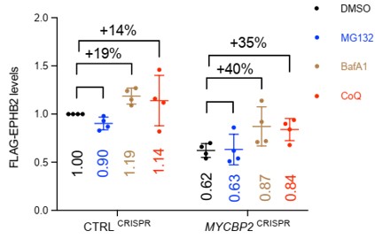
For each of the 4 replicates, the increase in EPHB2 levels by BafA1 compared to DMSO is as follows:
Author response table 1.

These values are not significantly different between CtrlCRISPR cells versus MYCBP2 CRISPR cells (p= 0.08, student’s t test). Similarly for the CoQ experiment. We now temper our conclusion for this experiment: Although the difference in percentage increase between CTRLCRISPR cells and MYCBP2CRISPR cells is not significant, this trend raises the possibility that the loss of MYCBP2 promotes EPHB2 receptor degradation through the lysosomal pathway (line 319). We also adjusted the section title (line 306).
7) While the C. elegans part is now MUCH better explained - we are not sure we understand the additional insight. The fact that vab-1 and glo4 double mutants are additive as are vab1 and fsn1, suggest they act in parallel (if the mutants are NULL, and not if they are hypomorphs, if one wants to be accurate) - how this relates to your story is unclear. The vab1/rpm1 double mutant is still uninformative and incomplete. rpm1 phenotype is so severe that nothing would make it more severe. We read the Jin paper that the authors directed to - nothing makes the rpm1 phenotype more severe. Yes, some DOWNSTREAM elements make the rpm1 phenotype LESS severe - this is not something you were testing, to the best of our knowledge. Rather, you wanted to see if rpm1 mutant resulted in stabilization of vab1 and thus suppression of vab1 phenotype - we are just not sure the system is amenable to test (actually reject) your hypothesis that Vab1 is degraded by rpm1. Also, assuming we are talking about NULLs, the fact that the rpm1 phenotype is WAY stronger than the vab1 mutant, suggests that rpm1 functions via multiple routes, adding even more complexity to the system. Given these results, despite the much improved clarity, we are still not sure that the worm data adds new insight, rather than potentially confusing the reader.
We realise that the genetic interactions between vab-1 and the RPM-1/MYCBP2 signalling network are complicated. However, we insist on keeping the data for the sake of its availability for future studies and completeness. We also think it is important for readers and the community to see these data, even if the authors and reviewers are not entirely in agreement about the importance/interpretation of experimental outcomes. It is our hope that the community will examine the results and draw their own conclusions.
A few points of clarification:
The C. elegans experiments were designed to test genetically if the vertebrate interactions between EPHB2 and MYCBP2 and its signalling network are conserved. We studied two kinds of interactions: (1) between vab-1 and RPM-1/MYCBP2 downstream proteins (GLO-4 and FSN-1) and (2) between vab-1 and rpm-1. For these studies, we used null alleles for vab-1, glo-4 and fsn-1 which is now noted on lines 440, 453, 475 and 859. Our findings are consistent with the VAB-1 Ephrin receptor functioning in parallel to known RPM-1 binding proteins. This is further supported by new data: vab-1; fsn-1 double mutants showed enhanced incidence of axon overextension defects using a second transgenic background, zdIs5 (Pmec-4::GFP), to visualize axon termination (Fig. 8F).
This second transgenic background also allowed us to generate new data to address your concerns about phenotypic saturation in rpm-1 mutants. To do this, we used the zdIs5 (Pmec4::GFP) genetic background, in which axon termination defects are not saturated in rpm-1 mutants (Fig. 8F) because they can be enhanced by other mutants such as cdc-42 and unc-33 (Fig. 7C, D, in Borgen et al. Development 144, 4658–4672 (2017), PMID 29084805). In this new background, we found that vab-1 loss of function fails to enhance the incidence of severe “hook” defects in rpm-1 mutants which is an indication that the two genes function in the same pathway. Importantly, prior studies in this background, also showed that mutants in the RPM-1 signalling network (e.g. fsn-1, glo-4 and ppm-2) do not enhance the incidence of severe “hook” defects as double mutants with rpm-1 compared to rpm-1 single mutants (Fig. 7B, ibid.).
To reflect these ideas more clearly, we revised the Results section pertaining to C. elegans genetics (starting on line 418) and tempered our discussion (lines 517). Basically, this section now says that we studied genetic interactions between vab-1 and the RPM-1/MYCBP2 signalling network. From these experiments we conclude that: (1) The enhancement of overextension defects in vab-1; glo-4 and vab-1; fsn-1 double mutants compared to single mutants indicates that VAB-1/EPHR functions in parallel to known RPM-1 binding proteins to facilitate axon termination, and (2) Since the vab-1; rpm-1 double mutants do not display an increased frequency or severity of overextension defects compared to rpm-1 single mutants, VAB-1 /EPHR functions in the same genetic pathway as RPM-1/MYCBP2.
The new genetic data included in this version were generated by Karla J. Opperman who is now included as a co-author.
Further corrections:
Author response image 4.
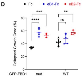
Because of the errors associated with quantifications in Fig. 3D (see above), we reviewed other quantification methodologies and noticed another discrepancy that required a correction. In the hippocampal neuron growth cone collapse assay shown in the previous version of Fig. 7 D (left), the growth cones were classified into three groups: 1, fully collapsed; 2, hard to tell, but not fully collapsed; 3, fan-shape cones. Two different quantifications were performed as follows: (1), number of fully collapsed cones divided by the numbers of all growth cones; (2), number of fully collapsed cones divided by [number of fully collapsed cones + fan-shape cones]. CC erroneously used the second method to generate Fig. 7D.
We think that the first method is more appropriate. Furthermore, since n=5 for the Fc and eB1-Fc conditions, but n=3 for the eB2-Fc condition, we decided to omit it. The final plot for figure 7D is the following:
Author response image 5.
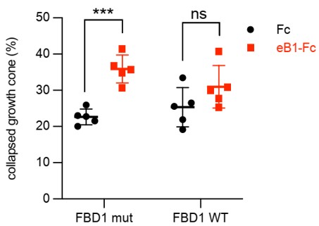
Our conclusion still stands that exogenous FBD1 WT overexpression impaired the growth cone collapse mediated by EphB.
Author response:
The following is the authors’ response to the original reviews.
Public Reviews:
Reviewer #1 (Public Review):
Summary:
In this paper, Steinemann et al. characterized the nature of stochastic signals underlying the trial-averaged responses observed in the lateral intraparietal cortex (LIP) of non-human primates (NHPs), while these performed the widely used random dot direction discrimination task. Ramp-up dynamics in the trial averaged LIP responses were reported in numerous papers before. However, the temporal dynamics of these signals at the single-trial level have been subject to debate. Using large-scale neuronal recordings with Neuropixels in NHPs, allows the authors to settle this debate rather compellingly. They show that drift-diffusion-like computations account well for the observed dynamics in LIP.
Strengths:
This work uses innovative technical approaches (Neuropixel recordings in behaving macaque monkeys). The authors tackle a vexing question that requires measurements of simultaneous neuronal population activity and hence leverage this advanced recording technique in a convincing way
They use different population decoding strategies to help interpret the results.
They also compare how decoders relying on the data-driven approach using dimensionality reduction of the full neural population space compare to decoders relying on more traditional ways to categorize neurons that are based on hypotheses about their function. Intriguingly, although the functionally identified neurons are a modest fraction of the population, decoders that only rely on this fraction achieve comparable decoding performance to those relying on the full population. Moreover, decoding weights for the full population did not allow the authors to reliably identify the functionally identified subpopulation.
Weaknesses:
No major weaknesses beyond a few, largely clarification issues, detailed below.
We thank Reviewer 1 (R1) for this summary. The revised manuscript incorporates R1’s suggestions, as detailed below.
Reviewer #2 (Public Review):
Steinemann, Stine, and their co-authors studied the noisy accumulation of sensory evidence during perceptual decision-making using Neuropixels recordings in awake, behaving monkeys. Previous work has largely focused on describing the neural underpinnings through which sensory evidence accumulates to inform decisions, a process which on average resembles the systematic drift of a scalar decision variable toward an evidence threshold. The additional order of magnitude in recording throughput permitted by the methodology adopted in this work offers two opportunities to extend this understanding. First, larger-scale recordings allow for the study of relationships between the population activity state and behavior without averaging across trials. The authors’ observation here of covariation between the trial-to-trial fluctuations of activity and behavior (choice, reaction time) constitutes interesting new evidence for the claim that neural populations in LIP encode the behaviorally-relevant internal decision variable. Second, using Neuropixels allows the authors to sample LIP neurons with more diverse response properties (e.g. spatial RF location, motion direction selectivity), making the important question of how decision-related computations are structured in LIP amenable to study. For these reasons, the dataset collected in this study is unique and potentially quite valuable.
However, the analyses at present do not convincingly support two of the manuscript’s key claims: (1) that ”sophisticated analyses of the full neuronal state space” and ”a simple average of Tconin neurons’ yield roughly equivalent representations of the decision variable; and (2) that direction-selective units in LIP provide the samples of instantaneous evidence that these Tconin neurons integrate. Supporting claim (1) would require results from sophisticated population analyses leveraging the full neuronal state space; however, the current analyses instead focus almost exclusively on 1D projections of the data. Supporting claim (2) convincingly would require larger samples of units overlapping the motion stimulus, as well as additional control analyses.
We thank the reviewer (R2) for their careful reading of our paper and the many useful suggestions.
As detailed below, the revised manuscript incorporates new control analyses, improved quantification, and statistical rigor, which now provide compelling support for key claim #1. We do not regard claim #2 as a key claim of the paper. It is an intriguing finding with solid support, worthy of dissemination and further investigation. We have clarified the writing on this matter.
Specific shortcomings are addressed in further detail below:
(1) The key analysis-correlation between trial-by-trial activity fluctuations and behavior, presented in Figure 5 is opaque, and would be more convincing with negative controls. To strengthen the claim that the relationship between fluctuations in (a projection of) activity and fluctuations in behavior is significant/meaningful, some evidence should be brought that this relationship is specific - e.g. do all projections of activity give rise to this relationship (or not), or what level of leverage is achieved with respect to choice/RT when the trial-by-trial correspondence with activity is broken by shuffling.
We do not understand why R2 finds the analysis opaque, but we are grateful for the lucid recommendations. The relationships between fluctuations in neural activity and behavior are indeed “specific” in the sense that R2 uses this term. In addition to the shuffle control, which destroys both relationships (Reviewer Figure 1), we performed additional control analyses that preserve the correspondence of neural signals and behavior on the same trial. We generated random coding directions (CDs) by establishing weight vectors that were either chosen from a standard normal distribution or by permuting the weights assigned to PC-1 in each session. The latter is the more conservative measure. Projections of the neural responses onto these random coding directions render 𝑆rand(𝑡). Specifically, the degree of leverage is effectively zero or greatly reduced. These analyses are summarized in a new Supplementary Figure S10. The bottom row of Figure S10 also addresses the question, “What degree of leverage and mediation would be expected for a theoretical decision variable?” This is accomplished by simulating decision variables using the drift-diffusion model fits in Figure 1c. The simulation is consistent with the leverage and (incomplete) mediation observed for the populations of Tcon neurons. For details see Methods, Simulated decision variables and Leverage of single-trial activity on behavior.
(2) The choice to perform most analysis on 1D projections of population activity is not wholly appropriate for this unique type of dataset, limiting the novelty of the findings, and the interpretation of similarity between results across choices of projection appears circular:
We disagree with the characterization of our argument as circular, but R2 raises several important points that will probably occur to other careful readers. We address them as subpoints 2.1–2.4, below. Importantly, we are neither claiming nor assuming that the LIP population activity is one-dimensional. We have revised the paper to avoid giving this impression. We are also not claiming that the average of Tin neurons (or the 1D projections) explains all features of the LIP population, nor would we expect it to, given the diversity of response fields across the population. Our objective is to identify the specific dimension within population activity that captures the decision variable (DV), which has been characterized successfully as a one-dimensional stochastic process—that is, a scalar function of time. We have endeavored to clarify our thinking on this point in the revised manuscript (e.g., lines 97–98, 103–104).
(2.1) The bulk of the analyses (Figure 2, Figure 3, part of Figure 4, Figure 5, Figure 6) operate on one of several 1D projections of simultaneously recorded activity. Unless the embedding dimension of these datasets really does not exceed 1 (dimensionality using e.g. participation ratio in each session is not quantified), it is likely that these projections elide meaningful features of LIP population activity.
We now report the participation ratio (4.4 ± 0.4, mean ± s.e. across sessions), and we state that the first 3 PCs explain 67.1±3.1% of the variance of time- and coherence-dependent signals used for the PCA. We agree that the 1D projections may elide meaningful features of LIP population activity. Indeed, we make this point through our analysis of the Min neurons. We do not claim that the 1D projections explain all of the meaningful features of LIP population activity. They do, however, reveal the decision variable, which is our main focus. These 1D signals contain features that correlate with events in the superior colliculus, summarized in Stine et al. (2023), attesting to their biological relevance.
(2.2) Further, the observed similarity of results across these 1D projections may not be meaningful/interpretable. First, the rationale behind deriving Sramp was based on the ramping historically observed in Tin neurons during this task, so should be expected to resemble Tin.
The Reviewer is correct that we would expect 𝑆ramp to resemble the ramping observed in Tin neurons. We refer to this approach as hypothesis-driven. It captures the drift component of drift-diffusion. It is true that the Tcon neurons exhibit such ramps in their trial average firing rates, but this does not guarantee in
that the single-trial population firing rates would manifest as drift-diffusion. Indeed Latimer et al. (2015) concluded that the ramp-like averages comprise stepping from a low to a high firing rate on each trial at a random time. Therefore, while R2 is right to characterize the similarity of Tcon to the ramp direction in in trial-averaged activity as unsurprising, their similarity on single trials is not guaranteed.
(2.3) Second, Tin comprises the largest fraction of the neuron groups sampled during most sessions, so SPC1 should resemble Tin too. The finding that decision variables derived from the whole population’s activity reduce essentially to the average of Tin neurons is thus at least in part ’baked in’ to the approach used for deriving the decision variables.
This is incorrect. The Tcon in neurons constitute only 14.5% of the population, on average, across the sessions (see Table 1). This misunderstanding might contribute to R2’s concern about the importance of these neurons in shaping PC1. It is not simply because they are over-represented. Also, addressing R2’s concern about circularity, we would like to remind R2 that the selection of Tin neurons was based only on their spatial selectivity in the delayed saccade task. We do not see how it could be baked-in/guaranteed that a simple average of these neurons (i.e. zero degrees of freedom) yields dynamics and behavioral correlations that match those produced by dimensionality-reduction techniques that (𝑖) have degrees of freedom equal to the number of neurons and (𝑖𝑖) are blind to the neurons’ spatial selectivity. We have additionally modified what is now Supplementary Figure S13 (old Supplementary Figure S8), which portrays the mean accuracy of choice decoders trained on the neural activity of all neurons, only Tin neurons, all but the Tin neurons, and all but Tin and Min neurons, respectively. Figure S13 now highlights how much more readily choice can be decoded from the small population of Tin neurons than the remainder of the population.
(2.4) The analysis presented in Figure S6 looks like an attempt to demonstrate that this isn’t the case, but is opaque. Are the magnitudes of weights assigned to units in Tin larger than in the other groups of units with preselected response properties? What is their mean weighting magnitude, in comparison with the mean weight magnitude assigned to other groups? What is the null level of correspondence observed between weight magnitude and assignment to Tin (e.g. a negative control, where the identities of units are scrambled)?
The revised Figure S6—what is now Figure S9—displays more clearly that the weights assigned to Tcon and Tips neurons (purple & yellow, respectively) are larger in magnitude than those assigned in in to other neurons (gray). Author response table 1 shows a more detailed breakdown of the groups. Note that the length of the vector of weights is one. We are unsure what R2 means by “the null level of correspondence.” Perhaps it helps to know that the mean weight of the “other neurons” is close to zero for all four coding directions. However, it is the overlap of the weights and the relative abundance of non-Tin neurons that is more germane to the point we are making. To wit, knowing the weight (or percentile) of a neuron is a poor predictor that it belongs to the Tin category. This point is most clearly supported by the logistic regression (Fig. S9, bottom row). In other words, the large group of non-Tin neurons contribute substantially to all four coding directions examined in Figure S9. Thus, the similarity between Tin neurons and PC1 is not simply due to an over-representation of Tin neurons as suggested in item 2.3.
Author response table 1.
Mean weights assigned to neuron classes in four coding directions.
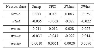
(3) The principal components analysis normalization procedure is unclear, and potentially incorrect and misleading: Why use the chosen normalization window (±25ms around 100ms after motion stimulus onset) for standardizing activity for PCA, rather than the typical choice of mean/standard deviation of activity in the full data window? This choice would specifically squash responses for units with a strong visual response, which distorts the covariance matrix, and thus the principal components that result. This kind of departure from the standard procedure should be clearly justified: what do the principal components look like when a standard procedure is used, and why was this insufficient/incorrect/unsuitable for this setting?
We used the early window because it is a robust measure of overall excitability, but we now use a more conventional window that spans the main epoch of our analyses, 200–600 ms after motion onset. This method yields results qualitatively similar to the original method. We are persuaded that this is the more sensible choice. We thank R2 for raising this concern.
(4) Analysis conclusions would generally be stronger with estimates of variability and control analyses: This applies broadly to Figures 2-6.
We have added estimates of variability and control analyses where appropriate.
Figure 2 shows examples of single-trial signals. The variability is addressed in Figure 3a and the new Supplementary Figure S5.
Figure 3 now contains error bars derived by bootstrapping (see Methods, Variance and autocorrelation of smoothed diffusion signals). We have also added Supplementary Figure S5, which substantiates the sublinearity claim using simulations.
Figure 4 (i) We now indicate the s.e.m. of decoding accuracy (across sessions) by the shading in Figure 4a. (ii) The black symbols in new Supplementary Figure S8 show the mean±s.e.m. for all pairwise comparisons shown in Figure 4d & e. (iii) Supplementary Figure S8 also summarizes two control analyses that deploy random coding directions (CDs) in neuronal state space. The upper row of Fig S9 compares the observed cosine similarity (CoSim)—between the CD identified by the graph title and the other four CDs labeled along the abscissa—with values obtained with 1000 random CDs established by random permutations of the weight assignments. The brown symbols are the mean±sdev of the CoSim (N=1000). The error bars are smaller than the symbols. We use the cumulative distribution of CoSim under permutation to estimate p-values (p<0.001 for all comparisons). We used a similar approach to estimate the distribution of the analogous correlation statistics between signals rendered by random directions in state space (Figure S8, lower row). For additional details, please see Methods, Similarity of single-trial signals.
Figure 5: The rigor of all claims associated with this figure is adduced from two control analyses and a simulation. The first control breaks the trial-by-trial correspondence between neural signals and behavior (Reviewer Figure 1). The second control shows that neural activity does not have substantial leverage on behavior when projected onto random directions in state space (Supplementary Figure S10, top). Simulations of decision variables using parameters derived from the fits to the behavioral data (Figure 1) support a degree of leverage and mediation comparable to the values observed for 𝑆Tincon (Supplementary Figure S10, bottom). For additional details, please see Methods (Leverage of single-trial activity on behavior) and the reply to item 1, above.
Figure 6: Panels c&d show estimates of variability across neurons and experimental sessions, respectively. The reported p-value is based on a permutation test (see Methods, Correlations between Min and Tconin ). The correlations shown in panel e (heatmap) are derived from pooled data across sessions. The reported p-value is based on a permutation test (see Methods, Correlations between Min and Tconin ).
Reviewer #3 (Public Review):
Summary:
The paper investigates which aspects of neural activity in LIP of the macaque give rise to individual decisions
(specificity of choice and reaction times) in single trials, by recording simultaneously from hundreds of neurons. Using a variety of dimensionality reduction and decoding techniques, they demonstrate that a population-based drift-diffusion signal, which relies on a small subset of neurons that overlap choice targets, is responsible for the choice and reaction time variability. Analysis of direction-selective neurons in LIP and their correlation with decision-related neurons (T con in [Tconin ] neurons ) suggests that evidence integration occurs within area LIP.
Strengths:
This is an important and interesting paper, which resolves conflicting hypotheses regarding the mechanisms that underlie decision-making in single trials. This is made possible by exploiting novel technology (Primatepixels recordings), in conjunction with state-of-the-art analyses and well-established dynamic random dot motion discrimination tasks.
General recommendations:
(1) Please tone down causal language. You presentcompelling correlativeevidencefor the idea thatLIP population activity encodes the drift-diffusion DV. We feel that claims beyond that (e.g., ”Single-trial drift-diffusion signals control the choice and decision time”) would require direct interventions, and are only partially supported by the current evidence. Further examples are provided in point 1) of Reviewer 1 below.
We have adopted the recommendation to “tone down the causal language.” Throughout the manuscript, we strive to avoid conveying the false impression that the present findings provide causal support for the decision mechanism. However, other causal studies of LIP support causality in the random dot motion task (Hanks et al., 2006; Jeurissen et al., 2022). It is therefore justifiable to use terms that imply causality in statements intended to convey hypotheses about mechanism. We agree that we should not give the false impression that the present support for said mechanism is adduced from causal perturbations in this study, as there were none.
(2) Please provide a commonly used, data-driven quantification of the dimensionality of the population activity – for example, using participation ratio or the number of PCs explaining 90 % of the variance. This will help readers evaluate the conclusions about the dimensionality of the data.
Principal component analysis reveals a participation ratio of 4.4 ± 0.4 (mean ±s.e., across sessions), and the first 3 PCs explain 67.1 ± 3.1 percent of the variance. The dimensionality of the data is low, but greater than one. We state this in Methods (Principal Component Analysis) and in Results (Single-trial drift-diffusion signals approximate the decision variable, lines 200–201).
(3) Please justify the normalization procedure used for PCA: Why use the chosen normalization window (±25ms around 100ms after motion stimulus onset) for standardizing activity for PCA, rather than the more common quantification of mean/standard deviation across the full data window? What do the first principal components look like when the latter procedure is used?
We now use a more conventional window that spans the main epoch of our analyses, 200–600 ms after motion onset. This method yields results qualitatively similar to the original method. We are persuaded that this is the more sensible choice.
(4) Please provide estimates of variability for variance and autocorrelation in Fig. 3 (e.g., through bootstrapping). Further, simulations could substantiate the claim about the expected sub-linearity at later time points (Fig. 3a) due to the upper stopping bound and limited firing rate range.
We thank the reviewers for these helpful recommendations. The revised Fig. 3 now contains error bars derived by bootstrapping (see Methods, Variance and autocorrelation of smoothed diffusion signals). We have also added Supplementary Figure S5, which substantiates the sub-linearity claim using simulations.
(5) Please add controls and estimates of variability for decoding across sessions in Fig. 4: what are the levels of within-trial correlation/cosine similarity for random coding directions? What is the variability in the estimates of values shown in a/d/e?
We have addressed each of these items. (1) Figure 4a now shows the s.e.m. of decoding accuracy (across sessions). (2) Regarding the variability of estimates shown in Figure 4d & e, the standard errors are displayed in the new supplementary Figure S8. It makes sense to show them there because there is no natural way to represent error on the heat maps in Figure 4, and Figure S8 concerns the comparison of the values in Figure 4d&e to values derived from random coding directions. (3) Random coding directions lead to values of cosine similarity and within-trial correlation that do not differ significantly from zero. We show this in several ways, summarized in our reply to Public Review item 4. Additional details are in the revised manuscript (Methods, Similarity of single-trial signals) and the new Supplementary Figure S8.
(6) Please perform additional analysis to strengthen the claim from Fig. 6, that Min represents the integrand and not the integral. The analysis in Fig. 6d could be repeated with the integral (cumulative sum) of the single-trial Min signals. Does this yield an increase in leverage over time?
The short answer is, yes in part. Reviewer Figure 2a provides support for leverage of the integral on choice, and this leverage, like 𝑆Tincon (t), increases as a function of time. The effect is present in all seven sessions that have both Mleftin and Mrightin neurons (all 𝑝 < 1𝑒 − 10). However, as shown in panel b, the same integral fails to demonstrate more than a hint of leverage on RT. All correlations are barely negative, and the magnitude does not increase as a function of time. We suspect—but cannot prove—that this failure arises because of limited power and the expected weak effect. Recall that the mediation analysis of RT is restricted to longer trials. Moreover, the correlation between the Min difference and the Tin signal is less than 0.1 (heatmap, Fig. 6e), implying that the Min difference explains less than 1% of the variance of 𝑆Tin(𝑡). We considered including Reviewer Figure 2 in the paper, but we feel it would be disingenuous (cherry-picking) to report only the positive outcome of the leverage on choice. If the editors feel strongly about it, we would be open to including it, but leaving these analyses out of the revised manuscript seems more consistent with our effort to deëmphasize this finding. In the future, we plan to record simultaneously from populations MT and LIP neurons (Min and Tin, of course) and optimize Min neuron yield by placing the RDM stimulus in the periphery.
(7) Please describe the complete procedure for determining spatially-selective activity. E.g.: What response epoch was used, what was the spatial layout of the response targets, were responses to all ipsi- vs contralateral targets pooled, what was the spatial distribution of response fields relative to the choice targets across the population?
We thank the reviewers for pointing out this oversight. We now explain this procedure in the Methods (lines 629–644):
Neurons were classified post hoc as Tin by visual-inspection of spatial heatmaps of neural activity acquired in the delayed saccade task. We inspected activity in the visual, delay, and perisaccadic epochs of the task. The distribution of target locations was guided by the spatial selectivity of simultaneously recorded neurons in the superior colliculus (see Stine 2023 for details). Briefly, after identifying the location of the SC response fields, we randomly presented saccade targets within this location and seven other, equally spaced locations at the same eccentricity. In monkey J we also included 1–3 additional eccentricities, spanning 5–16 degrees. Neurons were classified as Tin if they displayed a clear, spatially-selective response in at least one epoch to one of the two locations occupied by the choice targets in the main task. Neurons that switched their spatial selectivity in different epochs were not classified as Tin. The classification was conducted before the analyses of activity in the motion discrimination task. The procedure was meant to mimic those used in earlier single-neuron studies of LIP (e.g., Roitman & Shadlen 2002) in which the location of the choice targets was determined online by the qualitative spatial selectivity of the neuron under study. The Tcon neurons in the in present study were highly selective for either the contralateral or ipislateral choice target used in the RDM task (AUC = 0.89±0.01; 𝑝 < 0.05 for 97% of neurons, Wilcoxon rank sum test). Given the sparse sampling of saccade target locations, we are unable to supply a quantitative estimate of the center and spatial extent of the RFs.
(8) Please clarify if a neuron could be classified as both Tin and Min. Or were these categories mutually exclusive?
These categories are mutually exclusive. If a neuron has spatially-selective persistent activity, as defined by the method described above, it is classified as a Tin neuron and not as an Min neuron even if it also shows motion-selective activity during passive motion viewing. We now specify this in the Methods (lines 831–832).
Reviewer #1 (Recommendations For The Authors):
𝑅∗1.1a Causal language (Line 23-24): “population activity represents […] drift” and “we provide direct support for the hypothesis that drift-diffusion signal is the quantity responsible for the variability in choice and RT” reads at first sight as if the authors claim that they present evidence for a causal effect of LIP activity on choice. The authors areotherwisenuanced and carefultopointout thattheir evidence is correlational. What seems to be meant is that the population activity/drift-diffusion signal ”approximates the DV that gives rise to the choices […]” (cf. line 399). I would recommend using such alternative phrasing to avoid confusion (and the typically strong reactions by readers against misleading causal statements).
We have adopted the reviewer’s recommendation and have modified the text throughout to reduce causal language. See our response to General Recommendation 1.
𝑅∗1.1b Relatedly, any discussion about the possibility of LIP being causally involved in evidence integration (e.g. lines 429-445 [Au: now 462–478]) should also comment on the possibility of a distributed representation of the decision variable given that neural correlates of the DV have been reported in several areas including PFC, caudate and FEF.
We believe this is possible. However, we hope to avoid discussions about causality given that it is not a focus of the paper. Although it is somewhat tangential, we have shown elsewhere that LIP is causal in the sense that causal manipulations affect behavior, but it is also true that causality does not imply necessity, and similarly, lack of necessity does not imply “only correlation.” Regarding distributed representations, it is worth keeping in mind the cautionary counter-example furnished by the SC study (Stine et al., 2023). The firing rates measured by averaging over trials are similar in SC and LIP; both manifest as coherence and direction-dependent ramps, leading to the suggestion that they form a distributed representation of the decision variable. With single-trial resolution, we now know that LIP and SC exhibit distinct dynamics—drift-diffusion and bursting, respectively. It remains to be seen if single-trial resolution achievable by simultaneous Neuropixels recordings from prefrontal areas and LIP reveal shared or distinct dynamics.
𝑅∗1.2 How was the spatially selective activity determined? The classification of Tin neurons is critical to this study - how was their spatial selectivity determined? Please describe this in similar detail as the description of direction selectivity on lines 681-690 [Au: now 824–832]. E.g.: what response epoch was used, what was the spatial layout of the response targets, were responses to all ipsi- vs contralateral targets pooled, and what was the spatial distribution of response fields relative to the choice targets across the population?
We now explain the selection procedure in Methods (lines 629–644). Please see our reply to General Recommendation 7, above.
𝑅∗1.3 Could a neuron be classified as both Tin and Min, or were these categories mutually exclusive? Please clarify. (This goes beyond the scope of the current study: but did the authors find evidence for topographic organization or clustering of these categories of neurons?)
These categories are mutually exclusive. Please see our response to General Recommendation 8, above.
𝑅∗1.4 Contrary to the statement on line 121, the trial averages in Fig. 2a, 2b show coherence dependency at the time of the saccade in saccade-aligned traces for the coding strategies, except for STin (fig. 2c). Is this a result of the choice for t1 (= 0.1s)? (The authors may want to change their statement on line 121.) Relatedly, do the population responses for the two coding strategies Sramp and SPC1 depend on the epoch used to derive weights for individual neurons?
We have revised the description to accommodate R2’s observation. 𝑆ramp retains weak coherence-dependence before saccades towards the choice target contralateral to the recording site. This was true in four of the eight sessions. For 𝑆PC1, there is no longer a coherence dependency for the Tin choices, owing to the change in normalization method (see revised Figure 2b).
We also corrected an error in the Methods section. Specifically, the ramp ends at 𝑡1 \= 0.05 s before the time of the saccade, not 𝑡1 \= 0.1 s. While we no longer emphasize the similarity of traces aligned to saccade, it is reasonable to find issue with the observation that they retain a dependency on coherence (𝑆ramp only) because, according to theory, traces associated with Tin choices should reach a common positive threshold at decision termination. That said, for the Ramp direction there may be a reason to expect this discrepancy from theory. The deterministic part of drift-diffusion includes an urgency signal that confers positive convexity to the deterministic drift. This accelerating nonlinearity is not captured by the ramp, and it is more prominent at longer decision times, thus low coherences. We do not share this interpretation in the revised manuscript, in part because retention of coherence dependency is present in only half the sessions (see Reviewer Figure 3) The correction to the definition of 𝑡1 also provides an opportunity to address R2’s final question (“Relatedly,…?”). For 𝑆ramp this particular variation in 𝑡1 does not affect 𝑆ramp, and 𝑆PC1 no longer retains coherence dependency for Tin choices. Note that our choice of 𝑡0 and 𝑡1 is based on the empirical observation that the ramping activity in response averages of Tin neurons typically begins 200 ms after motion onset and ends 50–100 ms before initiation of the saccadic choice. The starting time (𝑡0) is also supported by the observation that the decoding accuracy of a choice-decoder begins to diverge from chance at this time (Figure 4a).
𝑅∗1.5 It is intriguing that Sramp and SPC1 show dynamics that look so similar (fig. 2a, 2b). How do the weights assigned to each neuron in both strategies compare across the population?
The weights assigned to each neuron are very similar across the two strategies as indicated by a cosine similarity (0.65 ± 0.04, mean ±s.e.m. across sessions).
𝑅∗1.6 Tin neurons, which show dynamics closely resembling different coding directions (fig. 2) and the decoders do not have weights that can distinguish them from the rest of the population in each of these analyses (fig. S7). Is it fair to interpret these findings as evidence for broad decision-related co-variability in the recorded neural population in LIP?
Yes, our results are consistent with this interpretation. However, it is worth reiterating that decoding performance drops considerably when Tin neurons are not included (see Supplementary Figure S13). Thus, this broad decision-related co-variability is present but weak.
𝑅∗1.7 It is intriguing that the decoding weights of the different decoders did not allow the authors to reliably identify Tin neurons. Could this be, in part, due to the low dimensionality of the population activity and task that the animals are presumably overtrained on? Or do the authors expect this finding to hold up if the population activity and task were higher dimensional?
Great question! We can only speculate, but it seems possible that a more complex, “higher dimensional” task could make it easier to identify Tin neurons. For example, a task with four choices instead of two may decrease correlations among groups of neurons with different response fields. We have added this caveat to the discussion (lines 459-–461). One minor semantic objection: The animal has learned to perform a highly contrived task at low signal-to-noise. The animal is well-trained, not over-trained.
𝑅∗1.8 Lines 135-137 [Au: now 141–142]: The similarity in the single trial traces from different coding strategies (fig. 2a-2c, left) is not as evident to me as the authors suggest. It might be worthwhile computing the correlation coefficients between individual traces for each pair of strategies and reporting the mean correlation to support the author’s point.
We report the mean correlation between single-trial signals generated by the chosen dimensionality reduction methods in Figure 4e. We show the variability in this measure in Supplementary Figure S8. We have also adjusted the opacity of the single-trial traces in Figure 2, left.
𝑅∗1.9 Minor/typos:
-line 74: consider additionally citing Hyafil et al. 2023.
-line 588: ”that were strongly correlated”?
-line 615: ”were the actual drift-diffusion process were...”.
-line 717: ”a causal influence” -> ”no causal influence”.
Fig. 6: panel labels e vs d are swapped between the figure and caption.
Fig. 3c: labels r1,3 & r2,3 are flipped.
We have addressed all of these items. Thank you.
Reviewer #2 (Recommendations For The Authors):
𝑅∗2.1 (Figure 2) Determine whether restricting the analysis to 1D projections of the data is a suitable approach given the actual dimensionality of the datasets being analyzed:
- Should show some quantification of the dimensionality of the recorded activity; could do this by quantifying the dimensionality of population activity in each session, e.g. with participation ratio or related measures (like # PCs to explain some high proportion of the variance, e.g. 90 %). If much of the variation is not described in 1 dimension, then the paper would benefit from some discussion/analysis of the signals that occupy the other dimensions.
We now report the participation ratio (4.4 ± 0.4, mean ±s.e. across sessions), and we state that the first 3 PCs explain 67.1 ± 3.1% of the variance of the time- and coherence-dependent signals used for the PCA (mean ±s.e). We agree that the 1D projections may elide meaningful features of LIP population activity. Indeed, we make this point through our analysis of the Min neurons. To reiterate our response above, we do not claim that the 1D projections explain all of the meaningful features of LIP population activity. They do, however, reveal the decision variable, which is our main focus. These 1D signals contain features that correlate with events in the superior colliculus, summarized in Stine et al. (2023), attesting to their biological relevance.
The Reviewer is correct that our approach presupposes a linear embedding of the 1D decision variable inthepopulationactivity. Inotherwords, anonlinearrepresentationofthe1Ddecisionvariableinpopulation activity could have an embedding dimensionality greater than 1, and there may well be a non-linear method that reveals this representation. To test this possibility, we decoded choice on each trial from population activity using (1) a linear decoder (logistic classifier) or (2) a multi-layer neural network, which can exploit non-linearities. We found that, for each session, the two decoders performed similarly: the neural network outperforms the logistic decoder (barely) in just one session. The analysis suggests that the assumption of linear embedding of the decision variable is justified. We hope this analysis convinces the reviewer that “sophisticated analyses of the full neuronal state space” and “a simple average of [Tcon ] neurons” do in indeed yield roughly equivalent representations of the decision variable. We have included the results of this analysis in Supplementary Figure S12. See also item 2 of the Public response.
𝑅∗2.2 (Figure 3) Add estimates of variability for variance and autocorrelation through time from single-trial signals:
– E.g. by bootstrapping. Would be helpful for making rigorous the discussion of when the deviation from the theory is outside what would be expected by chance, even if it doesn’t change the specific conclusions here.
– If possible, it would help (by simulations, or maybe an added reference if it exists) to substantiate the claim about the expected sub-linearity at later time-points (Figure 3a) due to the upper stopping bound and limited firing rate range.
We thank the reviewer for this helpful comment. The revised Fig. 3 now contains error bars derived by bootstrapping (see Methods, §Variance and autocorrelation of smoothed diffusion signals). We have also added Supplementary Figure S5, which substantiates the sub-linearity claim using simulations.
𝑅∗2.3 (Figure 4) Add controls and estimates of variability for decoding across sessions:
– As a baseline - what is the level of within-trial correlation/cosine similarity when random coding directions are used?
– What is the variability in the estimates of values shown in a/d/e?
We have addressed each of these items. (1) Figure 4a now shows the s.e.m. of decoding accuracy (across sessions). (2) Regarding the variability of estimates shown in Figure 4d & e, the standard errors are displayed in the new Supplementary Figure S8. It makes sense to show them there because (i) there is no natural way to represent error on the heat maps in Figure 4, and (ii) S8 concerns the comparison of the values in Figure 4d & e to values derived from random coding directions. (3) Random coding directions lead to values of cosine similarity and within-trial correlation that do not differ significantly from zero. We show this in several ways, summarized in our reply to Public Review item 4. Additional details are in the revised manuscript (Methods: Similarity of single-trial signals) and the new Supplementary Figure S8. We also provide this information in response to Recommendation 5, above.
𝑅∗2.4 (Figure 5) Add negative controls and significance tests to support claims about trends in leverage:
– What is the level of increase in leverage attained from random 1D projections of the data, or other projections where the prior would be no leverage?
– What is the range of leverage values fit for a simulated signal with a ground-truth of no trend?
We have added two control analyses. In addition to a shuffle control, which destroys the relationship (Review Figure 1) we performed additional analyses that preserve the correspondence of neural signals and behavior on the same trial. We generated random coding directions (CDs) by establishing weight-vectors that were either chosen from a Normal distribution or by permuting the weights assigned to PC-1 in each session. The latter is the more conservative measure. Projections of the neural responses onto these random coding directions render 𝑆rand(𝑡). Specifically, the degree of leverage is effectively zero or very much reduced. These analyses are summarized in a new Supplementary Figure S10. The distributions of our test statistics (e.g., leverage on choice and RT) under the variants of the null hypothesis also support traditional metrics of statistical significance. Figure S10 (bottom row) also provides an approximate answer to the question: What degree of leverage and mediation would be expected for a theoretical decision variable? Briefly, we simulated 60,000 trials using the race model that best fits the behavioral data of monkey M. For any noise-free representation of a Markovian integration process, the leverage of an early sample of the DV on behavior would be mediated completely by later activity as the latter sample—up to the time of commitment—subsumes all variability captured by the earlier sample. We, therefore, generated 𝑆sim(𝑡) by first subsampling the simulated data to match the trial numbers of each session. To evaluate a DV approximated from the activity of 𝑁 Tconin neurons per session rather than the true DV represented by the entire population, we generated 𝑁 noisy instantiations of the signal for each of the subsampled, simulated trials. The noisy decision variable, 𝑆sim (t) is the mean activity of these 𝑁 noise-corrupted signals. The simulation is consistent with the leverage and incomplete mediation observed for the populations of Tcon neurons. For in additional details, see Methods, §Leverage of single-trial activity on behavior) and Supplementary Figure S10, caption. See also our response to item 1 of the Public Response.
𝑅∗2.5 The analysis is performed across several signed coherence levels, with data detrended for each signed coherence and choice to enable comparison of fluctuations relative to the relevant baseline; are results similar for the different coherences?
The results are qualitatively similar for individual coherences. There is less power, of course, because there are fewer trials. The analyses cannot be performed for coherences ≥ 12.8% because there are not enough trials that satisfy the inclusion criteria (presence of left and right choice trials with RT ≤ 670 ms). Nonetheless, leverage on choice and RT is statistically significant for 27 of the 30 combinations of motion strengths < 12.8% × three signals (𝑆ramp, 𝑆PC1 and 𝑆Tin) × behavioral measures (RT and choice) (RT: all 𝑝 < 0.008, Fisher-z; choice: all 𝑝 < 0.05, t-test ). The three exceptions are trials with 6.4% coherence rightward motion, which do not correlate significantly with RT on leftward choice trials. Reviewer Figure 4 shows the results of the leverage and mediation analyses, using only the 0% coherence trials.
𝑅∗2.6 (Figure 6) Additional analysis to strengthen the claim that Min represents the integrand and not the integral:
a. Repeating the analysis in Figure 6d with the integral (cumulative sum) of the single-trial Min signals and instead observing a significant increase in leverage over time would be strong evidence for this interpretation. If you again see no increase, then it suggests that the activity of these units (while direction selective) may not be strongly yoked to behavior. This scenario (no increasing leverage of the integral of Min on behavior through time) also raises an intriguing alternative possibility: that the noise driving the ’diffusion’ of drift-diffusion here may originate in the integrating circuit, rather than just reflecting the complete integration of noise in the stream of evidence itself.
b. Repeating the analysis in Figure 6d with the projection of the M subspace onto its own first PC (e.g. take the union of units {Mrightin, Mleftin} [our
], do PCA just on those units’ single
trial activities, identify the first PC, and project those activities on that dimension to obtain SPC1-M.
c. Ameliorating the sample-size limitation by relaxing the criteria for inclusion in Min - performing the same analyses shown, but including all units with visual RFs overlapping the motion stimulus, irrespective of their direction selectivity.
a. Reviewer Figure 2a provides support for leverage of the integral on choice, and this leverage, like  , increases as a function of time. The effect is present in all seven sessions that have both
  and
and  neurons (all 𝑝 < 1𝑒 − 10). However, as shown in panel b, the same integral fails
to demonstrate more than a hint of leverage on RT (all correlations are negative) and the magnitude does not vary as a function of time. We suspect—but cannot prove—that this failure arises because of limited power and the expected weak effect. Recall that the mediation analysis of RT is restricted to longer trials and that the correlation between the Min difference and the signal is less than 0.1 over the heatmap in Fig. 6e, implying that the Min difference explains less than 1% of the variance of 𝑆Tin(𝑡). We considered including Reviewer Figure 2 in the paper, but we feel it would be disingenuous (cherrypicking) to report only the positive outcome of the leverage on choice. If the editors feel strongly about it, we would be open to including it, but leaving these analyses out of the revised manuscript seems more consistent with our effort to deëmphasize this finding. In the future, we plan to record simultaneously from populations MT and LIP neurons (Min and Tin, of course) and optimize Min neuron yield by placing the RDM stimulus in the periphery. We also provide this information in response to Recommendation (6) above.
b. We tried the R’s suggestion to apply PCA to the union of Min neurons , , fully expecting PC1 to comprise weights of opposite sign for the right and left preferring neurons, but that is not what we observed. Instead, the direction selectivity is distributed over at least two PCs. We think this is a reflection of the prominence of other signals, such as the strong visual response and normalization signals (see Shushruth et al., 2018). In the spirit of the R’s suggestion, we also established an “evidence coding direction” using a regression strategy similar to the Ramp CD applied to the union of Min neurons. The strategy produced a coding direction with opposite signed weights dominating the right and left subsets. The projection of the neural data on this evidence CD yields a signal similar to the difference variable used in Fig. 6e (i.e., signals that are approximately constant firing rates vs time and scale as a function of signed coherence). These unintegrated signals exhibit weak leverage on choice and RT, consistent with Figure 6d. However, the integrated signal has leverage on choice but not RT, similar to the integral of the difference signal in Reviewer Figure 2.
c. We do not understand the motivation for this analysis. We could apply PCA or dPCA (or the regression approach, described above) to the population of units with RFs that overlap the motion stimulus, but it is hard to see how this would test the hypothesis that direction-selective neurons similar to those in area MT supply the momentary evidence. As mentioned, we have very few Min neurons (as few as two in session 3). Future experiments that place the motion stimulus in the periphery would likely increase the yield of Min neurons and would be better suited to study this question. As such, we do not see the integrand-like responses of Min neurons as a major claim of the paper. Instead, we view it as an intriguing observation that deserves follow-up in future experiments, including simultaneous recordings from populations of MT and LIP neurons (Min and Tin, of course). We have softened the language considerably to make it clear that future work will be needed to make strong claims about the nature of Min neurons.
𝑅∗2.7 Other questions: Figure 2c is described as showing the average firing rate of units in Tconin on single trials, but must also incorporate some baseline subtraction (as the shown traces dip into negative firing rates). Whatbaselineissubtracted? Aretheseresidualsignals, asdescribedforlaterfigures, orisadifferent method used? (Presumably, a similar procedure is used also for Figure 2a/b, given that all single-trial traces begin at 0.). Is the baseline subtraction justified? If the dataset really does reflect the decision variable with single-trial resolution, eliminating the baseline subtraction when visualizing single-trial activity might actually help to make the point clearer: trials which (for any reason) begin with a higher projection on the particular direction that furnishes the DV would be predicted to reach the decision bound, at any fixed coherence, more quickly than trials with a smaller projection onto this direction.
We thank the reviewer for this comment. For each trial, the mean activity between 175 ms and 225 ms after motion onset was subtracted when generating the single-trial traces. The baseline subtraction was only applied for visualization to better portray the diffusion component in the signal. Unless otherwise indicated, all analyses are computed on non-baseline corrected data. We now describe in the caption of Figure 2 that “For visualization, single-trial traces were baseline corrected by subtracting the activity in a 50 ms window around 200 ms.” Examples of the raw traces used for all follow-up analyses are displayed in Reviewer Figure 6.
Reviewer #3 (Recommendations For The Authors):
I only have a few comments to make the paper more accessible:
𝑅∗3.1 I struggle to understand how the linear fitting from -1 to 1 was done. More detail about how the single cell single-trial activity was generated to possibly go from -1 to 1 or do I completely misunderstand the approach? I assume the data standardization does that job?
We have rephrased and added clarifying detail to the section describing the derivation of the ramp signal in the Methods (Ramp direction).
We applied linear regression to generate a signal that best approximates a linear ramp, on each trial, 𝑖, that terminates with a saccade to the choice-target contralateral to the hemisphere of the LIP recordings. The ramps are defined in the epoch spanning the decision time: each ramp begins at 𝑓𝑖(𝑡0) = −1, where 𝑡0 \= 0.2 s after motion onset, and ends at 𝑓𝑖(𝑡1) = 1, where 𝑡1 \= 𝑡sac − 0.05 s (i.e., 50 ms before saccade initiation). The ramps are sampled every 25 ms and concatenated using all eligible trials to construct a long saw-tooth function (see Supplementary Figure S2). The regression solves for the weights assigned to each neuron such that the weighted sum of the activity of all neurons best approximates the saw-tooth. We constructed a time series of standardized neural activity, sampled identically to the saw-tooth. The spike times from each neuron are represented as delta functions (rasters) and convolved with a non-causal 25 ms boxcar filter. The mean and standard deviation of all sampled values of activity were used to standardize the activity for each neuron (i.e., Z-transform). The coefficients derived by the regression establish the vector of weights that define 𝑆ramp. The algorithm ensures that the population signal 𝑆ramp(𝑡), but not necessarily individual neurons, have amplitudes ranging from approximately −1 to 1.
𝑅∗3.2 It is difficult to understand how the urgency signal is derived, to then generate fig S4.
The urgency signal is estimated by averaging 𝑆𝑥(𝑡) at each time point relative to motion onset, using only the 0% coherence trials. We have clarified this in the caption of Supplementary Figure S4.
Author response image 1.
Shuffle control for Fig. 5. Breaking the within-trial correspondence between neural signal, 𝑆(𝑡), and choice suppresses leverage to near zero.
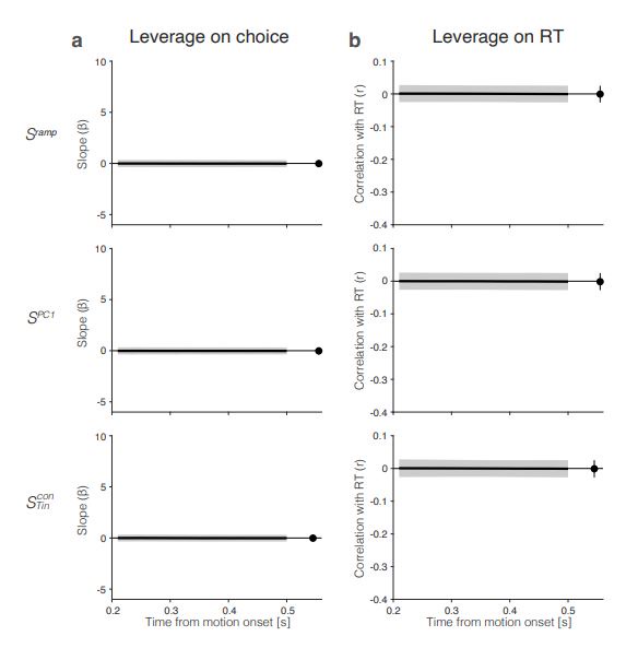
Author response image 2.
Leverage of the integrated difference signal  on choice and RT. Traces are the average leverage across seven sessions. Same conventions as in Figure 5.
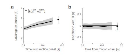
Author response image 3.
Trial-averaged 𝑆ramp activity during individual sessions. Same as Figure 2b for individual sessions for Monkey M (left) and Monkey J (right). The figure is intended to illustrate the consistency and heterogeneity of the averaged signals. For example, the saccade-aligned averages lose their association with motion strength before left (contra) choices in sessions 1, 2, 5, and 6 but retain the association in sessions 3, 4, 7, and 8.
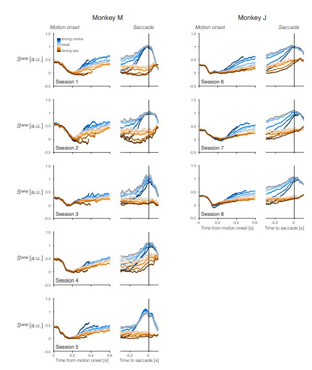
Author response image 4.
Drift-diffusion signals have measurable leverage on choice and RT even when only 0%-coherence trials are included in the analysis.
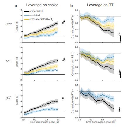
Author response image 5.
Raw single-trial activity for three types of population averages. Representative single-trial activity during the first 300 ms of evidence accumulation using two motion strengths: 0% and 25.6% coherence toward the left (contralateral) choice target. Unlike in Figure 2 in the paper, single-trial traces are not baseline corrected by subtracting the activity in a 50 ms window around 200 ms. We highlight a number of trials with thick traces and these are the same trials in each of the rows.
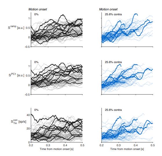
Author response:
The following is the authors’ response to the previous reviews.
Public Reviews:
Reviewer #1 (Public review):
Summary:
The investigators in this study analyzed the dataset assembly from 540 Salmonella isolates, and those from 45 recent isolates from Zhejiang University of China. The analysis and comparison of the resistome and mobilome of these isolates identified a significantly higher rate of cross-region dissemination compared to localized propagation. This study highlights the key role of the resistome in driving the transition and evolutionary history of S. Gallinarum.
Strengths:
The isolates included in this study were from 16 countries in the past century (1920 to 2023). While the study uses S. Gallinarun as the prototype, the conclusion from this work will likely apply to other Salmonella serotypes and other pathogens.
Thank you very much for your positive feedback. We recognize, as you noted, that emphasizing Salmonella enterica Serovar Gallinarum in the title may lead readers to perceive our methods and conclusions as overly restrictive. In light of your evaluation of our work, we have revised the title to: “Avian-specific Salmonella transition to endemicity is accompanied by localized resistome and mobilome interaction” We believe this final version not only reflects the applicability of our conclusions, as you appreciated, but also addresses your previous suggestion to highlight the resistome and mobilome.
Revisions in the manuscript Lines: 1-3
Weaknesses:
While the isolates came from 16 countries, most strains in this study were originally from China.
We believe that this issue was discussed in detail in our previous response. Although potential bias exists, we have minimized its impact by constructing the largest global S. Gallinarum genome dataset to date. In addition, we have further emphasized these limitations in the manuscript.
Comments on revisions:
This reviewer is happy with the detailed responses from the authors regarding revising this manuscript. I do not have further comments.
We greatly appreciate your positive feedback and are pleased that our responses have addressed your concerns.
Reviewer #2 (Public review):
Summary:
The authors sequence 45 new samples of S. Gallinarum, a commensal Salmonella found in chickens, which can sometimes cause disease. They combine these sequences with around 500 from public databases, determine the population structure of the pathogen, and coarse relationships of lineages with geography. The authors further investigate known anti-microbial genes found in these genomes, how they associate with each other, whether they have been horizontally transferred, and date the emergence of clades.
Strengths:
- It doesn't seem that much is known about this serovar, so publicly available new sequences from a high burden region are a valuable addition to the literature.
- Combining these sequences with publicly available sequences is a good way to better contextualise any findings.
- The genomic analyses have been greatly improved since the first version of the manuscript, and appropriately analyse the population and date emergence of clades.
- The SNP thresholds are contextualised in terms of evolutionary time.
- The importance and context of the findings are fairly well described.
Thank you so much for your thorough review and constructive comments on the manuscript.
Weaknesses:
- There are still a few issues with the genomic analyses, although they no longer undermine the main conclusions:
We are grateful for the valuable time and effort you have dedicated to improving our manuscript. In this revision, we have provided a point-by-point response to each of your concerns. Moreover, with the addition of new supplementary materials and modifications to the figures, we have re-examined and adjusted the numbering of figures and supplementary materials in the text to ensure they appear correctly in the manuscript.
(1) Although the SNP distance is now considered in terms of time, the 5 SNP distance presented still represents ~7yrs evolution, so it is unlikely to be a transmission event, as described. It would be better to use a much lower threshold or describe the interpretation of these clusters more clearly. Bringing in epidemiological evidence or external references on the likely time interval between transmissions would be helpful.
We sincerely thank you for highlighting this issue. We appreciate your concern regarding the use of a 5-SNP threshold to define a transmission event, especially given the approximate 7-year evolutionary timeframe. Considering our updated estimate for the evolutionary rate of S. Gallinarum (approximately 0.74 SNPs per year, with a 95% HPD range of 0.42 to 1.06), we have revised the manuscript to use a 2-SNP threshold (approximately representing less than two years of evolution) to better control the temporal span of transmission events. In addition, we have updated the manuscript to reflect this new threshold and demonstrated that the use of a more stringent SNP threshold does not affect the overall conclusions of the study.
Specifically, we adopted the newly established 2-SNP threshold to update Figure 3a and corresponding Supplementary Figure 8. The heatmap on the far right of New Figure 3a illustrates the SNP distances among 45 newly isolated S. Gallinarum strains from two locations in Zhejiang Province (Taishun and Yueqing). New Supplementary Figure 8 simulates potential transmission events between the bvSP strains isolated from Zhejiang Province (n=95) and those from other regions of China with available provincial information (n=435). These analyses collectively demonstrate the localized transmission patterns of bvSP within China.
For New Figure 3a, we found that even with the 2-SNP threshold, the number of potential transmission events among the 45 newly isolated S. Gallinarum strains from the two Zhejiang locations (Taishun and Yueqing) remains unchanged. In fact, we observed that the results from SNP tracing using an SNP threshold of less than 5 are consistent (see Author response image 1).
Author response image 1.
Clustering results of 45 newly isolated S. Gallinarum strains using different SNP thresholds of 1, 2, 3, 4, and 5 SNPs. The five subplots represent the clustering results under each threshold. Each point corresponds to an individual strain, and lines connect strains with potential transmission relationships.
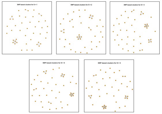
For New Supplementary Figure 8, we employed the 2-SNP threshold and found that the number of transmission events between the bvSP strains isolated from Zhejiang Province (n=95) and those from other Chinese provinces (n=435) decreased from 91 to 53. The names of the strains involved in these potential transmission events are listed in Supplementary Table 5.
Revisions in the manuscript
Lines: 352-357
Figures: Figure 3; Supplementary Figure 8
Table: Supplementary Table 5
(2) The HGT definition has not fundamentally been changed and therefore still has some issues, mainly that vertical evolution is still not systematically controlled for.
We sincerely thank you for highlighting this issue. We hope the following explanation will help clarify and improve our manuscript, as well as address your concerns.
In bacteria, mobile genetic elements (MGEs) such as plasmids, transposons, integrons, and prophages, as mentioned in our manuscript, are segments of DNA that encode enzymes and proteins responsible for mediating the movement of genetic material between bacterial genomes (commonly referred to as “jumping genes”). These MGEs contribute to the mechanisms of horizontal gene transfer (HGT) in Salmonella, including transduction (via prophages), conjugation (via plasmids), and transposition (via integrons and transposons) (Nat Rev Microbiol. 2005 Sep;3(9):722-32). These “jumping genes” can enable Salmonella to acquire additional antimicrobial resistance genes (ARGs), which may not only originate from other Salmonella strains but also from distantly related species.
To further address your concern regarding the systematic control of vertical evolution, we employed the HGTphyloDetect pipeline developed by Le Yuan et al. (Brief Bioinform. 2023 Mar 19;24(2):bbad035) to control for vertical evolution in the ARG sequences mentioned in our manuscript. We chose HGTphyloDetect because, as noted, "jumping genes" often occur among evolutionarily distant species, rendering the use of Gubbins potentially unsuitable for these distant HGT events.
Using the HGTphyloDetect pipeline, we extracted base sequences for the eight ARGs shown in Figure 6b with an HGT frequency greater than zero (bla<sup>TEM-1B</sup>, sul1, dfrA17, aadA5, sul2, aph(3’’)-Ib, tet(A), aph(6)-Id). For bla<sup>TEM-1B</sup>, sul1, dfrA17, aadA5, and sul2, the HGT frequency reached 100% across different isolates, indicating that these ARG sequences have a unique sequence type. In contrast, due to the ResFinder settings requiring both similarity and coverage to meet a minimum value of 90%, the base sequences for aph(3’’)-Ib, tet(A), and aph(6)-Id are not unique. Consequently, we applied the HGTphyloDetect pipeline individually to each sequence type of ARGs to verify their association with HGT events. Specifically, among 436 bvSP isolates collected in China, we identified two sequence types of aph(3’’)-Ib, four sequence types of tet(A), and three sequence types of aph(6)-Id.
Subsequently, to identify potential ARGs horizontally acquired from evolutionarily distant organisms, we queried the translated amino acid sequences of each ARG against the National Center for Biotechnology Information (NCBI) non-redundant protein database. We then evaluated whether these sequences were products of HGT by calculating Alien Index (AI) scores and out_perc values.
The calculation of AI score is as follows:

In this study, bbhG and bbhO represent the E-values of the best blast hit in ingroup and outgroup lineages, respectively. The outgroup lineage is defined as all species outside of the kingdom, while the ingroup lineage encompasses species within the kingdom but outside of the subphylum. An AI score ≥ 45 is considered a strong indicator that the gene in question is likely derived from an HGT event.
Regarding the calculation method for out_perc:

Finally, according to the definition provided by the HGTphyloDetect pipeline, ARGs with AI score ≥ 45 and out_perc ≥ 90% are presumed to be potential candidates for HGT from evolutionarily distant species. We have compiled the calculation results for the aforementioned genes in New Supplementary Table 9. The results indicate that all ARGs presented in Figure 6b, which exhibited a HGT frequency greater than zero, were acquired horizontally by S. Gallinarum. Based on these findings, we have revised the manuscript accordingly.
Revisions in the manuscript
Lines: 302-307; 616-650; 955-957
Table: Supplementary Table 9
Using a 5kb window is not sufficient, as LD may extend across the entire genome.
We agree with your point that linkage disequilibrium (LD) could influence the transmission of genes within chromosomal regions. LD can lead to the non-random cooccurrence of alleles at different loci within a population. Considering that horizontal gene transfer (HGT) events involving more distantly related ARGs may be accompanied by vertical propagation on chromosomes, and to simultaneously assess the impact of LD, we conducted two evaluations.
It is important to note that the following assessments are based on the assumption that plasmid replicons detected by PlasmidsFinder are part of self-replicating, extrachromosomal DNA.
(1) In the revised pipeline used to calculate ARG HGT frequencies, we categorized a total of 621 ARGs carried by 436 bvSP isolates collected in China and found that 415 of these ARGs were located on MGEs. We further investigated the distribution of these 415 ARGs across different MGEs, taking into account the complex nesting relationships among them. We observed that 90% of the ARGs (372/415) were located on plasmid contigs. It is important to clarify that this finding does not contradict our statement in the manuscript regarding plasmids and transposons as the primary reservoirs for resistome geo-temporal dissemination. This is because transposons, integrons, and prophages carrying ARGs can also be found on plasmids. Additionally, only 25 bvSG isolates from China contained ARGs, which were likely acquired via transposons or integrons located on the chromosome.
(2) In our manuscript, we searched for ARGs within a 5kb upstream and downstream region (a total of 10kb) of transposons and integrons (The BLASTn parameters used in the Bacant pipeline to identify transposons and integrons were set to a coverage threshold of 60%, rather than 100%). However, in light of the potential impact of LD on vertical transmission, we expanded our search to include a 10kb upstream and downstream range (a total of 20kb) for these 25 isolates. The decision to expand the search range to 10kb upstream and downstream range is based on the following two considerations: 1) Based on literature, we determined the overall lengths of the integrons and transposons carried by the 25 isolates (Tn801, Tn6205, Tn1721, In498, In1440, In473, and In282), and found that the maximum length of these elements is ~13.5 kb. Using a 10kb upstream and downstream threshold effectively covers these integrons/transposons. 2) The limitation posed by genomic fragmentation due to next-generation sequencing, which restrict the search range. We present the results of this expanded search for colocalization of ARGs with transposons and integrons at: Figshare: https://doi.org/10.6084/m9.figshare.28129130.v1
We found that these results were consistent with those obtained using the previous search range.
Taken together, these results suggest that although linkage disequilibrium may influence genetic processes within chromosomal regions—particularly for the few chromosomeassociated antibiotic resistance genes linked to integrons and transposons—the overall impact in our study is likely minimal. This conclusion is supported by the observation that 90% of the ARGs in our dataset are located on plasmids, and even an expanded search range does not alter this outcome. Additionally, by incorporating Alien Index scores and calculating out_perc, we can further confirm the occurrence of horizontal gene transfer events.
However, it is undeniable that other studies using our current pipeline may be affected. As a temporary remedial measure, we have included a note in the "README" file as below (https://github.com/tjiaa/Cal_HGT_Frequency):
“Note: Considering that ARGs located on the chromosome and carried by mobile genetic elements—such as integrons and transposons—may introduce potential computational errors, we recommend evaluating the number of ARGs associated with these elements on the chromosome during your analysis. If a majority of ARGs in your dataset fall into this category, we suggest using additional methods to evaluate the potential impact of linkage disequilibrium. Additionally, by modifying the “MGE_start” and “MGE_end” parameters in the “eLife_MGE_ARG_Co_location.ipynb” script, you can assess the distance between different ARGs and integrons or transposons on the chromosome. This approach will further aid in evaluating the impact of linkage disequilibrium on the genetic process.”
We believe this approach will assist researchers in further assessing the potential impact of vertical evolution and help other users determine whether additional methods are necessary to account for such effects.
As the authors have now run gubbins correctly, they could use the results from this existing analysis to find recent HGT.
We sincerely thank you for your valuable suggestion. Utilizing additional methods to predict potential horizontal gene transfer (HGT) events could indeed enhance the robustness of the results. However, "jumping genes" often occur among evolutionarily distant species, rendering the use of Gubbins potentially unsuitable for these distant HGT events.
Furthermore, the primary focus of our study is to identify HGT of antimicrobial resistance genes (ARGs) in the Salmonella genome driven by mobile genetic elements. Therefore, we employed the HGTphyloDetect pipeline developed by Le Yuan et al. (Brief Bioinform. 2023 Mar 19;24(2):bbad035) to control for vertical evolution in the ARG sequences. The specific computational methods and conclusions have been detailed above.
To definite mobilisation, perhaps a standard pipeline such (e.g. https://github.com/EBIMetagenomics/mobilome-annotation-pipeline) would be more convincing.
Thank you for your valuable suggestion. We agree that defining mobilization using a standardized pipeline can add rigor and clarity to our analysis. The pipeline you referenced (https://github.com/EBI-Metagenomics/mobilome-annotation-pipeline) is an excellent resource and provides a robust approach to the identification and annotation of mobile genetic elements.
We have examined and run this pipeline, which uses “IntegronFinder” and “ICEfinder” to detect integrons, “geNomad” to identify plasmids, and “geNomad” and “VIRify” to detect prophages. Our initial checks revealed that the numbers of integrons, plasmids, and prophages identified using this pipeline were consistent with those detected in our study. However, due to the significantly different output formats, the results from this pipeline could not be integrated with the pipeline we used for calculating HGT frequency.
We will incorporate the standardized pipeline you suggested in future studies to further improve the reliability of our findings.
(3) The invasiveness index is better described, but the authors still did not provide convincing evidence that the small difference is actually biologically meaningful (there was no statistical difference between the two strains provided in response Figure 6). What do other Salmonella papers using this approach find, and can their links be brought in? If there is still no good evidence, a better description of this difference would help make the conclusions better supported.
We sincerely appreciate your thoughtful feedback. The initial introduction of the invasiveness index in our manuscript aimed to quantitatively assess the differences in invasiveness between two geographically distinct strains of S. Gallinarum (isolated from Taishun and Yueqing) by comparing the degradation of 196 top predicted genes associated with invasiveness in their genomes. We found a highly significant statistical difference (P < 0.0001) in the invasiveness index between them.
Several studies have also employed the invasiveness index to predict biological relevance in Salmonella strains, and we believe these examples provide further context for our approach:
(1) Caisey V. Pulford et al, Nat Microbiol, 2021, used the same method to calculate the invasiveness index for Salmonella Typhimurium and employed it to characterize the invasiveness of different lineage strains. They found that Salmonella in Lineage-3 exhibited the highest invasiveness index, suggesting an adaptation from an intestinal to a systemic lifestyle. The authors noted, "Although the invasiveness index cannot yet be experimentally validated, Salmonella isolates with different invasiveness indices produce distinct clinical symptoms in a human population (BMC Med. 2020 Jul 17; 18(1):212)". They emphasized the necessity of developing more robust methods to measure Salmonella invasiveness.
(2) Sandra Van Puyvelde et al, Nat Commun, 2019, reported that Salmonella Typhimurium sequence type 313 (ST313) lineage II.1 exhibited a higher invasiveness index compared to lineage II, suggesting that the two lineages might have distinct adaptations to an invasive lifestyle. Further experiments demonstrated significant differences between these lineages in terms of biofilm formation (A red dry and rough (RDAR) assay) and metabolic capacity for carbon compounds.
(3) Wim L. Cuypers et al, Nat Commun, 2023, calculated the invasiveness index for 284 global Salmonella Concord strains across different lineages and found that Lineage-4 potentially exhibited the highest invasiveness.
Given these evidences, we acknowledge that no significant difference in mortality was observed between the L2b and L3b S. Gallinarum strains in 16-day-old SPF chicken embryos. Existing literature suggests that strains with higher invasiveness indices may still exhibit differences in biofilm formation and metabolic capacities, reflecting their adaptation to different host environments. As such, we maintain that the invasiveness index remains a valuable metric for evaluating the genomic differences between S. Gallinarum strains from Taishun and Yueqing. We plan to further investigate these differences through phenotypic experiments in our next research.
In the revised manuscript, we have added the following discussion along with additional references:
Lines 358-365: “Moreover, the invasiveness index of bvSP from Taishun and Yueqing suggests that different lineages of S. Gallinarum recovered from distinct regions may exhibit biological differences. Previous studies have shown that strains with higher invasiveness indexes tend to be more virulent in hosts (30, 31), potentially causing neurological or arthritic symptoms in S. Gallinarum infections. Furthermore, strains with varying invasiveness indexes have been confirmed to differ in their biofilm formation abilities and metabolic capacities for carbon compounds (32).”
Revisions in the manuscript:
Lines: 358-365, 806-827.
In summary, the analysis is broadly well described and feels appropriate. Some of the conclusions are still not fully supported, although the main points and context of the paper now appear sound.
Thank you so much for your positive evaluation of our work. We hope that the revised manuscript meets your expectations and offers a more accurate interpretation of our findings.
Recommendations for the authors:
Reviewer #2 (Recommendations for the authors):
This is a great improvement over the first version and I thank the authors for a thorough response, as well as changing their conclusions in response to their improvements.
Other small remaining issues:
Figure 3: Heatmap of SNPs is hard to read in grayscale. It also just represents the between clade distances already shown by the tree. It would be more useful to present intraclade distances only to see the SNP resolution _within_ each lineage. Using a better colour scheme would also help.
Thank you for your insightful comments and suggestions regarding Figure 3. We agree that the grayscale heatmap may present challenges in terms of visual clarity. To address this, we have updated the heatmap with a more distinct color gradient, ensuring better contrast and easier interpretation (New Figure 3).
Regarding your second suggestion: "It would be more useful to present intraclade distances only to see the SNP resolution within each lineage," we believe it is already addressed in the current version of New Figure 3. Specifically, the heatmap on the right side of New Figure 3 illustrates the SNP distances between S. Gallinarum isolates from Taishun and Yueqing, with the goal of demonstrating that genomic variation within isolates from a single region is generally smaller compared to those from different regions. In this figure, 45 newly isolated S. Gallinarum strains are categorized into two lineages: L2b and L3b. The heatmap on the right side of Figure 3 displays the SNP distances between all pairwise combinations of these 45 strains, where the intraclade distances are represented by the red regions (highlighting the pairwise distances within each lineage, specifically L3b and L2b, which are indicated by two triangles). The between-clade distances are shown by the blue regions.
We also believe in further exploring the intraclade distances across the entire dataset of 580 S. Gallinarum strains, as it could provide additional insights. However, this analysis would extend beyond the scope of the current section.
Revisions in the manuscript Line: 998
Figure: Figure 3
Please remove Figure 6c, it does not add anything to the paper and raises questions about performing this regression.
Thank you for pointing out this issue. We have removed Figure 6c and the corresponding description in the "Results" section from the manuscript (New Figure 6).
Revisions in the manuscript Lines: 316, 319, 1035-1041.
Figure: Figure 6
Again, thank you all for your time and efforts in reviewing our work. We believe the improved manuscript meets the high standards of the journal.
Author response:
The following is the authors’ response to the original reviews.
Public Reviews:
Reviewer #1 (Public Review):
Weaknesses & incompletely supported claims:
(1) A central mechanistic claim of the paper is that "DCP1a can regulate DCP2's cellular decapping activity by enhancing DCP2's affinity to RNA, in addition to bridging the interactions of DCP2 with other decapping factors. This represents a pivotal molecular mechanism by which DCP1a exerts its regulatory control over the mRNA decapping process." Similar versions of this claim are repeated in the abstract and discussion sections. However, this appears to be entirely at odds with the observation from in vitro decapping assays with immunoprecipitated DCP2 that showed DCP1 knockout does not significantly affect the enzymatic activity of DCP2 (Figures 2B-D; I note that there may be a very small change in DCP2 activity shown in panel C, but this may be due to slightly different amounts of immunoprecipitated DCP2 used in the assay, as suggested by panel D). If DCP1 pivotally regulates decapping activity by enhancing RNA binding to DCP2, why is no difference in decapping activity observed in the absence of DCP1?
Furthermore, the authors show only weak changes in relative RNA levels immunoprecipitated by DCP2 with versus without DCP1 (~2-3 fold change; consistent with the Valkov 2016 NSMB paper, which shows what looks like only modest changes in RNA binding affinity for yeast Dcp2 +/- Dcp1). Is the argument that only a 2-3 fold change in RNA binding affinity is responsible for the sizable decapping defects and significant accumulation of deadenylated intermediates observed in cells upon Dcp1 depletion? (and if so, why is this the case for in-cell data, but not the immunoprecipitated in vitro data?)
We appreciate the reviewer's thoughtful comments on our paper. The reviewer points out an apparent contradiction between the claim that DCP1a regulates DCP2's cellular decapping activity and the observation that knocking out DCP1a does not significantly affect DCP2's enzymatic activity in vitro. However, it is important to underscore the challenge of reconciling differences between in vitro and in vivo experiments in scientific research. Although in vitro systems provide a controlled environment, they have inherent limitations that often fail to capture the complexities of cellular processes. Our in vitro experiments used immunoprecipitated proteins to ensure the presence of relevant factors, but these experiments cannot fully replicate the precise stoichiometry and dynamic interactions present in a cellular environment. Furthermore, the limited volume in vitro can actually facilitate reactions that may not occur as readily in the complex and heterogeneous environment of a cell. Therefore, the lack of a significant difference in decapping activity observed in vitro does not necessarily negate the regulatory role of DCP1 in the cellular context. Rather, it underscores our previous oversight of DCP1's importance in the decapping process under in vitro conditions. The conclusions regarding DCP1's regulatory mechanisms remain valid and supported by the presented evidence, especially when considering the inherent differences between in vitro and in vivo experimental conditions. It is precisely because of these differences that we recognized our previous underestimation of DCP1's significance. Therefore, our subsequent experiments focused on elucidating DCP1's regulatory mechanisms in the decapping process
The authors acknowledge this apparent discrepancy between the in vitro DCP2 decapping assays and in-cell decapping data, writing: "this observation could be attributed to the inherent constraints of in vitro assays, which often fall short of faithfully replicating the complexity of the cellular environment where multiple factors and cofactors are at play. To determine the underlying cause, we postulated that the observed cellular decapping defect in DCP1a/b knockout cells might be attributed to DCP1 functioning as a scaffold." This is fair. They next show that DCP1 acts as a scaffold to recruit multiple factors to DCP2 in cells (EDC3, DDX6, PatL1, and PNRC1 and 2). However, while DCP1 is shown to recruit multiple cofactors to DCP2 (consistent with other studies in the decapping field, and primarily through motifs in the Dcp1 C-terminal tail), the authors ultimately show that *none* of these cofactors are actually essential for DCP2-mediated decapping in cells (Figures 3A-F). More specifically, the authors showed that the EVH1 domain was sufficient to rescue decapping defects in DCP1a/b knockout cells, that PNRC1 and PNRC2 were the only cofactors that interact with the EVH1 domain, and finally that shRNA-mediated PNRC1 or PNCR2 knockdown has no effect on in-cell decapping (Figures 3E and F). Therefore, based on the presented data, while DCP1 certainly does act as a scaffold, it doesn't seem to be the case that the major cellular decapping defect observed in DCP1a/b knockout is due to DCP1's ability to recruit specific cofactors to DCP2.
The findings that none of the decapping cofactors recruited by DCP1 to DCP2 are essential for decapping in cells further underscore the complexity of the decapping process in vivo. This observation suggests that while DCP1's scaffolding function is crucial for recruiting cofactors, the decapping process likely involves additional layers of regulation that are not fully captured by our current understanding of DCP1. Furthermore, the reviewer mentions that the observed changes in RNA binding affinity (approximately 2-3 fold) in our in vitro experiments seem relatively modest. While these changes may appear insignificant in vitro, their cumulative impact in the dynamic cellular environment could be substantial. Even minor perturbations in RNA binding affinity can trigger cascading effects, leading to significant changes in decapping activity and the accumulation of deadenylated intermediates upon Dcp1 depletion. Cellular processes involve complex networks of interrelated events, and small molecular changes can result in amplified biological outcomes. The subtle molecular variations observed in vitro may translate into significant phenotypic outcomes within the complex cellular environment, underscoring the importance of DCP1a's regulatory role in the cellular decapping process.
So as far as I can tell, the discrepancy between the in vitro (DCP1 not required) and in-cell (DCP1 required) decapping data, remains entirely unresolved. Therefore, I don't think that the conclusions that DCP1 regulates decapping by (a) changing RNA binding affinity (authors show this doesn't matter in vitro, and that the change in RNA binding affinity is very small) or (b) by bridging interactions of cofactors with DCP2 (authors show all tested cofactors are dispensable for robust in-cell decapping activity), are supported by the evidence presented in the paper (or convincingly supported by previous structural and functional studies of the decapping complex).
We have addressed the reconciliation of differences between in vitro and in vivo experiments in the revised manuscript and emphasized the importance of considering cellular interactions when interpreting our findings.
(2) Related to the RNA binding claims mentioned above, are the differences shown in Figure 3H statistically significant? Why are there no error bars shown for the MBP control? (I understand this was normalized to 1, but presumably, there were 3 biological replicates here that have some spread of values?). The individual data points for each replicate should be displayed for each bar so that readers can better assess the spread of data and the significance of the observed differences. I've listed these points as major because of the key mechanistic claim that DCP1 enhances RNA binding to DCP2 hinges in large part on this data.
Thank you for your feedback. Regarding your comments on the statistical significance of the differences shown in Figure 3H and the absence of error bars for the MBP control, we will address these concerns in the revised manuscript. We’ll include individual data points for the three biological replicates and corresponding statistical analysis to more clearly demonstrate the data spread and significance of the observed differences.
(3) Also related to point (1) above, the kinetic analysis presented in Figure 2C shows that the large majority of transcript is mostly decapped at the first 5-minute timepoint; it may be that DCP2-mediated decapping activity is actually different in vitro with or without DCP1, but that this is being missed because the reaction is basically done in less than 5 minutes under the conditions being assayed (i.e. these are basically endpoint assays under these conditions). It may be that if kinetics were done under conditions to slow down the reaction somewhat (e.g. lower Dcp2 concentration, lower temperatures), so that more of the kinetic behavior is captured, the apparent discrepancy between in vitro and in-cell data would be much less. Indeed, previous studies have shown that in yeast, Dcp1 strongly activates the catalytic step (kcat) of decapping by ~10-fold, and reduces the KM by only ~2 fold (Floor et al, NSMB 2010). It might be beneficial to use purified proteins here (only a Western blot is used in Figure 2D to show the presence of DCP2 and/or DCP1, but do these complexes have other, and different, components immunoprecipitated along with them?), if possible, to better control reaction conditions.
This contradiction between the in vitro and in-cell decapping data undercuts one of the main mechanistic takeaways from the first half of the paper. This needs to be addressed/resolved with further experiments to better define the role of DCP1-mediated activation, or the mechanistic conclusions significantly changed or removed.
We genuinely appreciate the reviewer’s insightful comments on the kinetic analysis presented in Figure 2C. Your astute observation regarding the potential influence of reaction duration on the interpretation of in vitro decapping activity, especially in the absence of DCP1, is well-received. The time-sensitive nature of our experiments, as you rightly pointed out, might not fully capture the nuanced kinetic behaviors. In addition, the DCP2 complex purified from cells could not be precisely quantified. In response to your suggestion, we attempted to purify human DCP2 protein from E. coli; however, regrettably, the purified protein failed to exhibit any enzymatic activity. This disparity may be attributed to species differences.
Considering the reviewer’s valuable insights, our revised manuscript emphasized that purified DCP2 from cells exhibits activity regardless of the presence of DCP1. This adjustment aims to provide a clearer perspective on our findings and to better align with the nuances of our experimental design and the meticulous consideration of the results.
(4) The second half of the paper compares the transcriptomic and metabolic profiles of DCP1a versus DCP1b knockouts to reveal that these target a different subset of mRNAs for degradation and have different levels of cellular metabolites. This is a great application of the DCP1a/b KO cells developed in this paper and provides new information about DCP1a vs b function in metazoans, which to my knowledge has not really been explored at all. However, the analysis of DCP1 function/expression levels in human cancer seems superficial and inconclusive: for example, the authors conclude that "...these findings indicate that DCP1a and DCP1b likely have distinct and non-redundant roles in the development and progression of cancer", but what is the evidence for this? I see that DCP1a and b levels vary in different cancer cell types, but is there any evidence that these changes are actually linked to cancer development, progression, or tumorigenesis? If not, these broader conclusions should be removed.
Thank you to the reviewer for pointing out that such a description may be misleading. We have removed our previous broader conclusion and revised our sentences. To further explore the potential impact of DCP1a and DCP1b on cancer progression, we examined the association between the expression levels of DCP1a and DCP1b and progression-free interval (PFI). We have incorporated this information into our revised manuscript.
(5) The authors used CRISPR-Cas9 to introduce frameshift mutations that result in premature termination codons in DCP1a/b knockout cells (verified by Sanger sequencing). They then use Western blotting with DCP1a or DCP1b antibodies to confirm the absence of DCP1 in the knockout cell lines. However, the DCP1a antibody used in this study (Sigma D5444) is targeted to the C-terminal end of DCP1a. Can the authors conclusively rule out that the CRISPR/Cas-generated mutations do not result in the production of truncated DCP1a that is just unable to be detected by the C-terminally targeted antibody? While it is likely the introduced premature termination codon in the DCP1a gene results in nonsense-mediated decay of the resulting transcript, this outcome is indeed supported by the knockout results showing large defects in cellular decapping which can be rescued by the addition of the EVH1 domain, it would be better to carefully validate the success of the DCP1a knockout and conclusively show no truncated DCP1a is produced by using N-terminally targeted DCP1a antibodies (as was the case for DCP1b).
Thank you for your insightful comment regarding the validation of our DCP1a/b knockout cell line. We acknowledge your point about the DCP1a C-terminal targeting of the Sigma D5444 antibody used in our Western blot analysis. We agree that we cannot definitively rule out the possibility of truncated DCP1a protein production solely based on the lack of full-length protein detection. To address this limitation, we utilized a commercial information available N-terminally targeted DCP1a antibody (aviva ARP39353_T100) in a Western blot analysis. This will allow us to comprehensively detect any truncated protein fragments remaining after the CRISPR-Cas9-generated frameshift mutation.
Some additional minor comments:
• More information would be helpful on the choice of DCP1 truncation boundaries; why was 1-254 chosen as one of the truncations?
Thank you for the reviewer's comment and suggestion. Regarding the choice of DCP1 1-254 truncation boundaries based on the predicted structure from AlphaFoldDB (A0A087WT55). We will include this information in the revised manuscript.
• Figure S2D is a pretty important experiment because it suggests that the observed deadenylated intermediates are in fact still capped; can a positive control be added to these experiments to show that removal of cap results in rapid terminator-mediated degradation?
Unfortunately, due to our institution's current laboratory safety policies, we are unable to perform experiments involving the use of radioactive isotopes such as 32P. Therefore, while adding the suggested positive control experiment to demonstrate rapid RNA degradation upon decapping would further validate our interpretation, we regret that we cannot carry out this experiment at the moment. However, the observed deadenylated intermediates in Figure S2D match the predicted size of capped RNA fragments, and not the expected sizes of degradation products after decapping. Furthermore, previous literature has well-established that for these types of RNAs, decapping leads directly to rapid 5' to 3' exonuclease-mediated degradation, without producing stable deadenylated intermediates. Thus, we believe that the current data is sufficient to support our conclusion that the deadenylated intermediates retain the 5' cap structure.
Reviewer #2 (Public Review):
Weaknesses:
The direct targets of DCP1a and/or DCP1b were not determined as the analysis was restricted to RNA-seq to assess RNA abundance, which can be a result of direct or indirect regulation by DCP1a/b.
Thank you for raising this important point. In our study, we acknowledge that the use of RNA-seq to assess RNA abundance provides a broad overview of the regulatory impacts of DCP1a and DCP1b. This method captures changes in RNA levels that may arise from both direct and indirect regulatory actions of these proteins. While we did not directly determine the targets of DCP1a and DCP1b, the data obtained from our RNA-seq analysis serve as a foundational step for future targeted experiments, which could include techniques such as RIP-seq, to delineate the direct targets of DCP1a and DCP1b more precisely. We believe that our current findings contribute valuable information to the field and pave the way for these subsequent analyses.
P-bodies appear to be larger in human cells lacking DCP1a and DCP1b but a lack of image quantification prevents this conclusion from being drawn.
Thank you for the reviewer’s valuable feedback. We have addressed the reviewer’s concern regarding P-bodies' size in human cells lacking DCP1a and DCP1b. We have now performed image quantification and can confirm that P-bodies are indeed larger in these cells.
The lack of details in the methodology and figure legends limit reader understanding.
We acknowledge the reviewer's concerns regarding the level of detail provided in the methodology and figure legends. To address this, we are committed to enhancing both sections with additional details and clarifications in our revised manuscript. Thank you for bringing this to our attention.
Recommendations for the authors:
Reviewer #1 (Recommendations For The Authors):
(1) To me, the second half of the paper comparing DCP1a and DCP1b is in many ways distinct from the first half and could stand on its own as an interesting paper if this comparative analysis is explored a little deeper (maybe by validating some of the differences in decay observed for individual mRNAs targeted by DCP1a versus DCP1b, by measuring and comparing the decay rates of some individual transcripts under differential control by DCP1a vs b?), and revising the conclusions about links to cancer as mentioned above. I think these later comparative results in the paper present the most new and interesting data concerning DCP1 function in humans (especially since I think the mechanistic conclusions from the first half aren't well supported yet or are at least inconsistent), but when I read these later sections of the paper I struggle to understand the key takeaways from the transcriptomic and metabolomic data.
Thank you for the reviewer's suggestions. Estimating the decay rates of individual transcripts within the transcriptomes of DCP1a_KO, DCP1b_KO, and wild type can provide insight into the direct targets of DCP1a or DCP1b. However, this requires either time-series RNA-seq or specialized sequencing technologies such as Precision Run-On sequencing (PRO-seq) or RNA Approach to Equilibrium Sequencing (RATE-Seq). Unfortunately, we lack the necessary dataset in our project to estimate the decay rates for the potential targets identified in our RNA-seq data. Despite this limitation, we acknowledge the potential of this approach in identifying the true targets of DCP1a and DCP1b and have included this idea in our discussion.
(2) I think it would be helpful to add a little more descriptive or narrative language to the figure legends (I know some of them are already quite long!) so that readers can follow the general idea of the experiment through the figure legend as well as the main text; as written, the figure legends are mostly exclusively technical details, so it can be hard to parse what experiment is being carried out in some cases.
Thank you for the reviewer’s suggestion, we will strive to improve the language of the figure legends to include technical details while clearly conveying the main idea of the experiment. We will ensure that the language of the figure legends is more readable and comprehensible so that readers can more easily parse what experiment is being carried out.
Reviewer #2 (Recommendations For The Authors):
Suggestions for improved or additional experiments, data, or analyses:
The use of RNA-seq to measure RNA abundance in DCP1a and/or b knockout cells can give some insight into both the indirect and direct effects of DCP1a/b on gene expression but cannot identify the direct targets of these genes. Rather, global analysis of RNA stability or capturing uncapped RNA decay intermediates would allow the authors to conclude they have identified direct targets of DCP1a and/or b. Without such analyses, the interpretation of these data should be scaled back to clearly state that RNA levels can be altered through indirect effects of DCP1a/b absence throughout the text.
We appreciate the reviewer's suggestion. We have modified our sentences to emphasize that the dysregulated genes could be caused by both direct and indirect effects.
A control/randomly generated gene list should be analyzed for GO terms to determine whether the enrichment of cancer-related pathways in the differentially expressed genes in the DCP1a/b knockout cells is meaningful.
Thank you for the reviewer's comment. We shuffled our gene list and reperformed the pathway enrichment analysis in Figure 4C and 4D 1,000 times. We focused on the following cancer-related pathways: E2F targets, MTORC1 signaling, G2M checkpoint, MYC target V1, EMT transition, KRAS signaling DN, P53 pathway, and NOTCH signaling pathways. We then calculated how many times the q-values obtained from the shuffled gene list were more significant than the q-value obtained from our real data. In four of the eight pathways (E2F targets, MTORC1 signaling, G2M checkpoint, and MYC target v1), none of the shuffled gene lists resulted in a q-value smaller than the real one. In the other four pathways (EMT transition, KRAS signaling DN, P53 pathway, and NOTCH signaling pathways), the q-values were smaller than the real q-value 2, 11, 4, and 4 times out of the 1000 shuffles. Based on the shuffled results, we conclude that the transcriptome of DCP1a/b knockout cells is statistically enriched in these cancer-related pathways.
Author response image 1.
Distribution of q-values resulting from the Gene Set Enrichment Analysis (GSEA) conducted on 1,000 shuffled gene lists for eight cancer-related pathways. The q-values derived from Figure 4C and 4D are indicated by red (DCP1a_KO) and blue (DCP1b_KO) dashed lines, respectively. Some q-values derived from Figure 4C are too small to be labeled on the plots, such as in E2F targets (q value: 5.87E-07), MTORC1 signaling (q values: 6.59E-07 and 1.58E-06 for DCP1a_KO and DCP1b_KO, respectively), MYC target V1 (q value: 0.004644174 for DCP1a_KO), etc. The numbers x/1000 indicate how often the shuffled q-values were smaller than the real q-value out of 1,000 permutations.
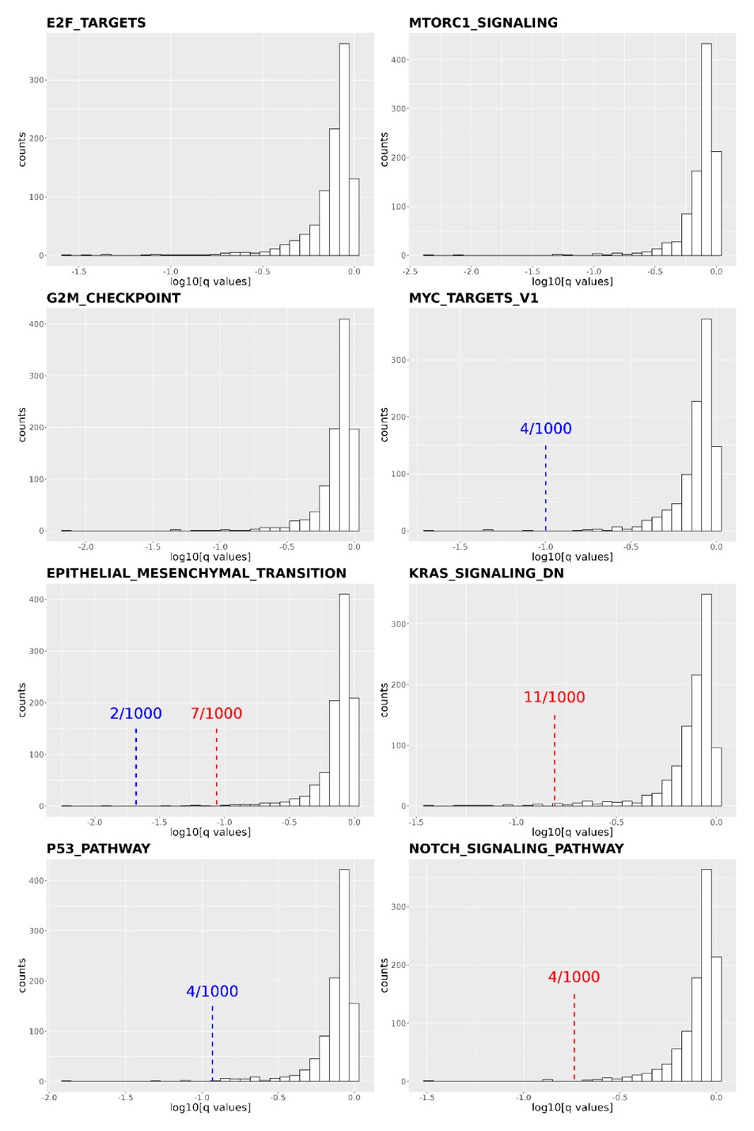
Comparisons of the DCP1a and/or b knockout RNA-seq results should be done to published datasets such as those published by Luo et al., Cell Chemical Biology (2021) to determine whether there are common targets with DCP2 and validate the reported findings.
Thank you for reviewer’s suggestion. We compared the upregulated genes from DCP1a_KO, DCP1b_KO, and DCP1a/b_KO cell lines with the 91 targets of DPC2 identified by Luo et al. in Cell Chemical Biology (2021). Only EPPK1 was found to be overlapped between the potential DCP1b_KO targets and the targets of DCP2. No genes were found to be overlapped between the potential DCP1a_KO targets and the targets of DCP2. However, three genes, TES, PAX6, and C18orf21, were found to be overlapped between the significantly upregulated DEGs of DCP1a/b_KO and the targets of DCP2. We have included this information in the discussion section.
The RNA tethering assays are not clear and are difficult to interpret without further controls to delineate the polyadenylated and deadenylated species.
Thank you for the reviewer’s feedback. We acknowledge that the reviewer might harbor some doubts regarding the outcomes of the RNA tethering assays. Nonetheless, this methodology is well-established and has also found extensive application across many studies. We are committed to enhancing the clarity of our experiment’s details and results within the figure legends and textual descriptions.
The representative images of p-bodies clearly show that DCP1a/b KO cells have larger p-bodies than the wild-type cells. The authors should quantify p-body size in each image set as the current interpretation of the data is that there is no difference in size or number of p-bodies, but the data suggest otherwise.
Thank you very much for the reviewer’s insightful comments and for drawing our attention to the need to quantify p-body sizes in DCP1a/b KO and wild-type cells. We agree with the reviewer’s assessment that the representative images suggest a difference in p-body size between DCP1a/b KO cells and wild-type cells, which we initially overlooked. We will revise our manuscript accordingly to include these findings, ensuring that our interpretation of the data aligns with the observed differences.
Statistical analysis of the Figure 2C results should be included because the difference between the wild-type and Dco1a/b KO cells with GFP-DCP2 looks significantly different but is interpreted in the text as not significant.
Thank you for pointing out the need for a statistical analysis of the results shown in Figure 2C. We acknowledge that the visual difference between the wild-type and Dco1a/b KO cells with GFP-DCP2 suggests a significant variation, which may not have been clearly communicated in our text. We will conduct the necessary statistical analysis to substantiate the observations made in Figure 2C. Furthermore, we would like to emphasize that our primary focus was to demonstrate that purified DCP2 within cells retains its activity even in the absence of DCP1. This critical point will be highlighted and clarified in the revised version of our manuscript to prevent any misunderstanding.
Recommendations for improving the writing and presentation:
Additional context including what is known about the role of dcp1 in decapping from the decades of work in yeast and other model organisms should be incorporated into the introduction and discussion sections.
Thank you for the reviewer’s suggestion. We will incorporate additional context about the function and significance of DCP1 in decapping processes within our revised manuscript's introduction and discussion sections.
Details should be provided within the figure legends and methods section on experimental approaches and the number of replicates and statistical analyses used throughout the manuscript. For example, it is not clear whether western blots or RNA-IP experiments were performed more than once as representative images are shown.
Thank you for the reviewer’s suggestion. In the figure legends and methods section, we will provide more details about the experimental methods, number of replicates, and statistical analyses. Regarding the Western blots and RNA-IP experiments the reviewer mentioned, we performed multiple experiments and presented representative images in the manuscript. We will clarify this in the revised manuscript to eliminate potential confusion.
The rationale for performing metabolic profiling is not clear.
We appreciate the reviewer's thoughtful feedback. The rationale behind conducting metabolic profiling in our study is rooted in its efficacy as a valuable tool for deciphering the consequences of specific gene mutations, particularly those closely associated with phenotypic changes or final metabolic pathways. Our objective is to utilize metabolic profiling to unravel the distinct biofunctions of DCP1a and DCP1b. By employing this approach, we aim to gain insights into the intricate metabolic alterations that result from the absence of these genes, thereby enhancing our understanding of their roles in cellular processes. We recognize the necessity of clearly presenting this rationale and promise to bolster the articulation of these points in the revised version of our manuscript to ensure the clarity and transparency of our research motivation.
Details in the methods section should be included for the CRISPR/Cas9-mediated gene editing validation. The Sangar sequencing results presented in Figure S1b should be explained. The entire western blot(s) should be shown in Figure S1A to give confidence the Dcp1a/b KO cells are not expressing truncated proteins and the epitopes of the antibodies used to detect Dcp1a/b should be described. The northern blot probes should be described and sequences included. The transcriptomics method should be detailed.
Thank you for your feedback, in the revised manuscript we will detail the CRISPR/Cas9 gene editing validation, explain the Sanger sequencing results in Figure S1b, show the full Western blot in Figure S1A to confirm that the Dcp1a/b knockout cells are not expressing truncated proteins, describe the Northern blot probes used, and detail the transcriptomics method, all to ensure clarity and comprehensiveness in our experimental procedures and results.
A diagram showing the RNA tethering assays with labels corresponding to all blots/gels should be provided.
Thank you for your suggestion. We will provide a diagram showing the RNA tethering assays with labels corresponding to all blots/gels in our revised manuscript. This will help readers better understand our experimental design and results.
The statement, "This suggests that the disruption of the decapping process in DCP1a/b-knockout cells results in the accumulation of unprocessed mRNA intermediates" regarding the results of the RNA-seq assay is not supported by the evidence as RNA-seq does not measure RNA decay intermediates or RNA decay rates.
Thank you for the reviewer’s comment. We agree with that RNA-seq experiments indeed do not directly measure RNA decay intermediates or RNA decay rates. Our statement could have caused confusion, and we have therefore removed this sentence from the manuscript.
Minor corrections to the text and figures:
Figure S6A is uninterpretable as presented.
Thank you for the reviewer’s valuable feedback. We have taken note and made improvements. We have simplified Figure S6A to enhance its interpretability, hoping that the current version will make it easier for the readers to understand.
Author response:
The following is the authors’ response to the previous reviews
Overview of reviewer's concerns after peer review:
As for the initial submission, the reviewers' unanimous opinion is that the authors should perform additional controls to show that their key findings may not be affected by experimental or analysis artefacts, and clarify key aspects of their core methods, chiefly:
(1) The fact that their extremely high decoding accuracy is driven by frequency bands that would reflect the key press movements and that these are located bilaterally in frontal brain regions (with the task being unilateral) are seen as key concerns,
The above statement that decoding was driven by bilateral frontal brain regions is not entirely consistent with our results. The confusion was likely caused by the way we originally presented our data in Figure 2. We have revised that figure to make it more clear that decoding performance at both the parcel- (Figure 2B) and voxel-space (Figure 2C) level is predominantly driven by contralateral (as opposed to ipsilateral) sensorimotor regions. Figure 2D, which highlights bilateral sensorimotor and premotor regions, displays accuracy of individual regional voxel-space decoders assessed independently. This was the criteria used to determine which regional voxel-spaces were included in the hybridspace decoder. This result is not surprising given that motor and premotor regions are known to display adaptive interhemispheric interactions during motor sequence learning [1, 2], and particularly so when the skill is performed with the non-dominant hand [3-5]. We now discuss this important detail in the revised manuscript:
Discussion (lines 348-353)
“The whole-brain parcel-space decoder likely emphasized more stable activity patterns in contralateral frontoparietal regions that differed between individual finger movements [21,35], while the regional voxel-space decoder likely incorporated information related to adaptive interhemispheric interactions operating during motor sequence learning [32,36,37], particularly pertinent when the skill is performed with the non-dominant hand [38-40].”
We now also include new control analyses that directly address the potential contribution of movement-related artefact to the results. These changes are reported in the revised manuscript as follows:
Results (lines 207-211):
“An alternate decoder trained on ICA components labeled as movement or physiological artefacts (e.g. – head movement, ECG, eye movements and blinks; Figure 3 – figure supplement 3A, D) and removed from the original input feature set during the pre-processing stage approached chance-level performance (Figure 4 – figure supplement 3), indicating that the 4-class hybrid decoder results were not driven by task-related artefacts.”
Results (lines 261-268):
“As expected, the 5-class hybrid-space decoder performance approached chance levels when tested with randomly shuffled keypress labels (18.41%± SD 7.4% for Day 1 data; Figure 4 – figure supplement 3C). Task-related eye movements did not explain these results since an alternate 5-class hybrid decoder constructed from three eye movement features (gaze position at the KeyDown event, gaze position 200ms later, and peak eye movement velocity within this window; Figure 4 – figure supplement 3A) performed at chance levels (cross-validated test accuracy = 0.2181; Figure 4 – figure supplement 3B, C). “
Discussion (Lines 362-368):
“Task-related movements—which also express in lower frequency ranges—did not explain these results given the near chance-level performance of alternative decoders trained on (a) artefact-related ICA components removed during MEG preprocessing (Figure 3 – figure supplement 3A-C) and on (b) task-related eye movement features (Figure 4 – figure supplement 3B, C). This explanation is also inconsistent with the minimal average head motion of 1.159 mm (± 1.077 SD) across the MEG recording (Figure 3 – figure supplement 3D).“
(2) Relatedly, the use of a wide time window (~200 ms) for a 250-330 ms typing speed makes it hard to pinpoint the changes underpinning learning,
The revised manuscript now includes analyses carried out with decoding time windows ranging from 50 to 250ms in duration. These additional results are now reported in:
Results (lines 258-261):
“The improved decoding accuracy is supported by greater differentiation in neural representations of the index finger keypresses performed at positions 1 and 5 of the sequence (Figure 4A), and by the trial-by-trial increase in 2-class decoding accuracy over early learning (Figure 4C) across different decoder window durations (Figure 4 – figure supplement 2).”
Results (lines 310-312):
“Offline contextualization strongly correlated with cumulative micro-offline gains (r = 0.903, R<sup>2</sup> = 0.816, p < 0.001; Figure 5 – figure supplement 1A, inset) across decoder window durations ranging from 50 to 250ms (Figure 5 – figure supplement 1B, C).“
Discussion (lines 382-385):
“This was further supported by the progressive differentiation of neural representations of the index finger keypress (Figure 4A) and by the robust trial-bytrial increase in 2-class decoding accuracy across time windows ranging between 50 and 250ms (Figure 4C; Figure 4 – figure supplement 2).”
Discussion (lines 408-9):
“Offline contextualization consistently correlated with early learning gains across a range of decoding windows (50–250ms; Figure 5 – figure supplement 1).”
(3) These concerns make it hard to conclude from their data that learning is mediated by "contextualisation" ---a key claim in the manuscript;
We believe the revised manuscript now addresses all concerns raised in Editor points 1 and 2.
(4) The hybrid voxel + parcel space decoder ---a key contribution of the paper--- is not clearly explained;
We now provide additional details regarding the hybrid-space decoder approach in the following sections of the revised manuscript:
Results (lines 158-172):
“Next, given that the brain simultaneously processes information more efficiently across multiple spatial and temporal scales [28, 32, 33], we asked if the combination of lower resolution whole-brain and higher resolution regional brain activity patterns further improve keypress prediction accuracy. We constructed hybrid-space decoders (N = 1295 ± 20 features; Figure 3A) combining whole-brain parcel-space activity (n = 148 features; Figure 2B) with regional voxel-space activity from a datadriven subset of brain areas (n = 1147 ± 20 features; Figure 2D). This subset covers brain regions showing the highest regional voxel-space decoding performances (top regions across all subjects shown in Figure 2D; Methods – Hybrid Spatial Approach).
[…]
Note that while features from contralateral brain regions were more important for whole-brain decoding (in both parcel- and voxel-spaces), regional voxel-space decoders performed best for bilateral sensorimotor areas on average across the group. Thus, a multi-scale hybrid-space representation best characterizes the keypress action manifolds.”
Results (lines 275-282):
“We used a Euclidian distance measure to evaluate the differentiation of the neural representation manifold of the same action (i.e. - an index-finger keypress) executed within different local sequence contexts (i.e. - ordinal position 1 vs. ordinal position 5; Figure 5). To make these distance measures comparable across participants, a new set of classifiers was then trained with group-optimal parameters (i.e. – broadband hybrid-space MEG data with subsequent manifold extraction (Figure 3 – figure supplements 2) and LDA classifiers (Figure 3 – figure supplements 7) trained on 200ms duration windows aligned to the KeyDown event (see Methods, Figure 3 – figure supplements 5). “
Discussion (lines 341-360):
“The initial phase of the study focused on optimizing the accuracy of decoding individual finger keypresses from MEG brain activity. Recent work showed that the brain simultaneously processes information more efficiently across multiple—rather than a single—spatial scale(s) [28, 32]. To this effect, we developed a novel hybridspace approach designed to integrate neural representation dynamics over two different spatial scales: (1) whole-brain parcel-space (i.e. – spatial activity patterns across all cortical brain regions) and (2) regional voxel-space (i.e. – spatial activity patterns within select brain regions) activity. We found consistent spatial differences between whole-brain parcel-space feature importance (predominantly contralateral frontoparietal, Figure 2B) and regional voxel-space decoder accuracy (bilateral sensorimotor regions, Figure 2D). The whole-brain parcel-space decoder likely emphasized more stable activity patterns in contralateral frontoparietal regions that differed between individual finger movements [21, 35], while the regional voxelspace decoder likely incorporated information related to adaptive interhemispheric interactions operating during motor sequence learning [32, 36, 37], particularly pertinent when the skill is performed with the non-dominant hand [38-40]. The observation of increased cross-validated test accuracy (as shown in Figure 3 – Figure Supplement 6) indicates that the spatially overlapping information in parcel- and voxel-space time-series in the hybrid decoder was complementary, rather than redundant [41]. The hybrid-space decoder which achieved an accuracy exceeding 90%—and robustly generalized to Day 2 across trained and untrained sequences— surpassed the performance of both parcel-space and voxel-space decoders and compared favorably to other neuroimaging-based finger movement decoding strategies [6, 24, 42-44].”
Methods (lines 636-647):
“Hybrid Spatial Approach. First, we evaluated the decoding performance of each individual brain region in accurately labeling finger keypresses from regional voxelspace (i.e. - all voxels within a brain region as defined by the Desikan-Killiany Atlas) activity. Brain regions were then ranked from 1 to 148 based on their decoding accuracy at the group level. In a stepwise manner, we then constructed a “hybridspace” decoder by incrementally concatenating regional voxel-space activity of brain regions—starting with the top-ranked region—with whole-brain parcel-level features and assessed decoding accuracy. Subsequently, we added the regional voxel-space features of the second-ranked brain region and continued this process until decoding accuracy reached saturation. The optimal “hybrid-space” input feature set over the group included the 148 parcel-space features and regional voxelspace features from a total of 8 brain regions (bilateral superior frontal, middle frontal, pre-central and post-central; N = 1295 ± 20 features).”
(5) More controls are needed to show that their decoder approach is capturing a neural representation dedicated to context rather than independent representations of consecutive keypresses;
These controls have been implemented and are now reported in the manuscript:
Results (lines 318-328):
“Within-subject correlations were consistent with these group-level findings. The average correlation between offline contextualization and micro-offline gains within individuals was significantly greater than zero (Figure 5 – figure supplement 4, left; t = 3.87, p = 0.00035, df = 25, Cohen's d = 0.76) and stronger than correlations between online contextualization and either micro-online (Figure 5 – figure supplement 4, middle; t = 3.28, p = 0.0015, df = 25, Cohen's d = 1.2) or micro-offline gains (Figure 5 – figure supplement 4, right; t = 3.7021, p = 5.3013e-04, df = 25, Cohen's d = 0.69). These findings were not explained by behavioral changes of typing rhythm (t = -0.03, p = 0.976; Figure 5 – figure supplement 5), adjacent keypress transition times (R2 = 0.00507, F[1,3202] = 16.3; Figure 5 – figure supplement 6), or overall typing speed (between-subject; R2 = 0.028, p \= 0.41; Figure 5 – figure supplement 7).”
Results (lines 385-390):
“Further, the 5-class classifier—which directly incorporated information about the sequence location context of each keypress into the decoding pipeline—improved decoding accuracy relative to the 4-class classifier (Figure 4C). Importantly, testing on Day 2 revealed specificity of this representational differentiation for the trained skill but not for the same keypresses performed during various unpracticed control sequences (Figure 5C).”
Discussion (lines 408-423):
“Offline contextualization consistently correlated with early learning gains across a range of decoding windows (50–250ms; Figure 5 – figure supplement 1). This result remained unchanged when measuring offline contextualization between the last and second sequence of consecutive trials, inconsistent with a possible confounding effect of pre-planning [30] (Figure 5 – figure supplement 2A). On the other hand, online contextualization did not predict learning (Figure 5 – figure supplement 3). Consistent with these results the average within-subject correlation between offline contextualization and micro-offline gains was significantly stronger than withinsubject correlations between online contextualization and either micro-online or micro-offline gains (Figure 5 – figure supplement 4).
Offline contextualization was not driven by trial-by-trial behavioral differences, including typing rhythm (Figure 5 – figure supplement 5) and adjacent keypress transition times (Figure 5 – figure supplement 6) nor by between-subject differences in overall typing speed (Figure 5 – figure supplement 7)—ruling out a reliance on differences in the temporal overlap of keypresses. Importantly, offline contextualization documented on Day 1 stabilized once a performance plateau was reached (trials 11-36), and was retained on Day 2, documenting overnight consolidation of the differentiated neural representations.”
(6) The need to show more convincingly that their data is not affected by head movements, e.g., by regressing out signal components that are correlated with the fiducial signal;
We now include data in Figure 3 – figure supplement 3D showing that head movement was minimal in all participants (mean of 1.159 mm ± 1.077 SD). Further, the requested additional control analyses have been carried out and are reported in the revised manuscript:
Results (lines 204-211):
“Testing the keypress state (4-class) hybrid decoder performance on Day 1 after randomly shupling keypress labels for held-out test data resulted in a performance drop approaching expected chance levels (22.12%± SD 9.1%; Figure 3 – figure supplement 3C). An alternate decoder trained on ICA components labeled as movement or physiological artefacts (e.g. – head movement, ECG, eye movements and blinks; Figure 3 – figure supplement 3A, D) and removed from the original input feature set during the pre-processing stage approached chance-level performance (Figure 4 – figure supplement 3), indicating that the 4-class hybrid decoder results were not driven by task-related artefacts.” Results (lines 261-268):
“As expected, the 5-class hybrid-space decoder performance approached chance levels when tested with randomly shuffled keypress labels (18.41%± SD 7.4% for Day 1 data; Figure 4 – figure supplement 3C). Task-related eye movements did not explain these results since an alternate 5-class hybrid decoder constructed from three eye movement features (gaze position at the KeyDown event, gaze position 200ms later, and peak eye movement velocity within this window; Figure 4 – figure supplement 3A) performed at chance levels (cross-validated test accuracy = 0.2181; Figure 4 – figure supplement 3B, C). “
Discussion (Lines 362-368):
“Task-related movements—which also express in lower frequency ranges—did not explain these results given the near chance-level performance of alternative decoders trained on (a) artefact-related ICA components removed during MEG preprocessing (Figure 3 – figure supplement 3A-C) and on (b) task-related eye movement features (Figure 4 – figure supplement 3B, C). This explanation is also inconsistent with the minimal average head motion of 1.159 mm (± 1.077 SD) across the MEG recording (Figure 3 – figure supplement 3D). “
(7) The offline neural representation analysis as executed is a bit odd, since it seems to be based on comparing the last key press to the first key press of the next sequence, rather than focus on the inter-sequence interval
While we previously evaluated replay of skill sequences during rest intervals, identification of how offline reactivation patterns of a single keypress state representation evolve with learning presents non-trivial challenges. First, replay events tend to occur in clusters with irregular temporal spacing as previously shown by our group and others. Second, replay of experienced sequences is intermixed with replay of sequences that have never been experienced but are possible. Finally, and perhaps the most significant issue, replay is temporally compressed up to 20x with respect to the behavior [6]. That means our decoders would need to accurately evaluate spatial pattern changes related to individual keypresses over much smaller time windows (i.e. - less than 10 ms) than evaluated here. This future work, which is undoubtably of great interest to our research group, will require more substantial tool development before we can apply them to this question. We now articulate this future direction in the Discussion:
Discussion (lines 423-427):
“A possible neural mechanism supporting contextualization could be the emergence and stabilization of conjunctive “what–where” representations of procedural memories [64] with the corresponding modulation of neuronal population dynamics [65, 66] during early learning. Exploring the link between contextualization and neural replay could provide additional insights into this issue [6, 12, 13, 15].”
(8) And this analysis could be confounded by the fact that they are comparing the last element in a sequence vs the first movement in a new one.
We have now addressed this control analysis in the revised manuscript:
Results (Lines 310-316)
“Offline contextualization strongly correlated with cumulative micro-offline gains (r = 0.903, R<sup>2</sup> = 0.816, p < 0.001; Figure 5 – figure supplement 1A, inset) across decoder window durations ranging from 50 to 250ms (Figure 5 – figure supplement 1B, C). The offline contextualization between the final sequence of each trial and the second sequence of the subsequent trial (excluding the first sequence) yielded comparable results. This indicates that pre-planning at the start of each practice trial did not directly influence the offline contextualization measure [30] (Figure 5 – figure supplement 2A, 1st vs. 2nd Sequence approaches).”
Discussion (lines 408-416):
“Offline contextualization consistently correlated with early learning gains across a range of decoding windows (50–250ms; Figure 5 – figure supplement 1). This result remained unchanged when measuring offline contextualization between the last and second sequence of consecutive trials, inconsistent with a possible confounding effect of pre-planning [30] (Figure 5 – figure supplement 2A). On the other hand, online contextualization did not predict learning (Figure 5 – figure supplement 3). Consistent with these results the average within-subject correlation between offline contextualization and micro-offline gains was significantly stronger than within-subject correlations between online contextualization and either micro-online or micro-offline gains (Figure 5 – figure supplement 4).”
It also seems to be the case that many analyses suggested by the reviewers in the first round of revisions that could have helped strengthen the manuscript have not been included (they are only in the rebuttal). Moreover, some of the control analyses mentioned in the rebuttal seem not to be described anywhere, neither in the manuscript, nor in the rebuttal itself; please double check that.
All suggested analyses carried out and mentioned are now in the revised manuscript.
eLife Assessment
This valuable study investigates how the neural representation of individual finger movements changes during the early period of sequence learning. By combining a new method for extracting features from human magnetoencephalography data and decoding analyses, the authors provide incomplete evidence of an early, swift change in the brain regions correlated with sequence learning…
We have now included all the requested control analyses supporting “an early, swift change in the brain regions correlated with sequence learning”:
The addition of more control analyses to rule out that head movement artefacts influence the findings,
We now include data in Figure 3 – figure supplement 3D showing that head movement was minimal in all participants (mean of 1.159 mm ± 1.077 SD). Further, we have implemented the requested additional control analyses addressing this issue:
Results (lines 207-211):
“An alternate decoder trained on ICA components labeled as movement or physiological artefacts (e.g. – head movement, ECG, eye movements and blinks; Figure 3 – figure supplement 3A, D) and removed from the original input feature set during the pre-processing stage approached chance-level performance (Figure 4 – figure supplement 3), indicating that the 4-class hybrid decoder results were not driven by task-related artefacts.”
Results (lines 261-268):
“As expected, the 5-class hybrid-space decoder performance approached chance levels when tested with randomly shuffled keypress labels (18.41%± SD 7.4% for Day 1 data; Figure 4 – figure supplement 3C). Task-related eye movements did not explain these results since an alternate 5-class hybrid decoder constructed from three eye movement features (gaze position at the KeyDown event, gaze position 200ms later, and peak eye movement velocity within this window; Figure 4 – figure supplement 3A) performed at chance levels (cross-validated test accuracy = 0.2181; Figure 4 – figure supplement 3B, C). “
Discussion (Lines 362-368):
“Task-related movements—which also express in lower frequency ranges—did not explain these results given the near chance-level performance of alternative decoders trained on (a) artefact-related ICA components removed during MEG preprocessing (Figure 3 – figure supplement 3A-C) and on (b) task-related eye movement features (Figure 4 – figure supplement 3B, C). This explanation is also inconsistent with the minimal average head motion of 1.159 mm (± 1.077 SD) across the MEG recording (Figure 3 – figure supplement 3D).“
and to further explain the proposal of offline contextualization during short rest periods as the basis for improvement performance would strengthen the manuscript.
We have edited the manuscript to clarify that the degree of representational differentiation (contextualization) parallels skill learning. We have no evidence at this point to indicate that “offline contextualization during short rest periods is the basis for improvement in performance”. The following areas of the revised manuscript now clarify this point:
Summary (Lines 455-458):
“In summary, individual sequence action representations contextualize during early learning of a new skill and the degree of differentiation parallels skill gains. Differentiation of the neural representations developed during rest intervals of early learning to a larger extent than during practice in parallel with rapid consolidation of skill.”
Additional control analyses are also provided supporting a link between offline contextualization and early learning:
Results (lines 302-318):
“The Euclidian distance between neural representations of Index<sub>OP1</sub> (i.e. - index finger keypress at ordinal position 1 of the sequence) and Index<sub>OP5</sub> (i.e. - index finger keypress at ordinal position 5 of the sequence) increased progressively during early learning (Figure 5A)—predominantly during rest intervals (offline contextualization) rather than during practice (online) (t = 4.84, p < 0.001, df = 25, Cohen's d = 1.2; Figure 5B; Figure 5 – figure supplement 1A). An alternative online contextualization determination equaling the time interval between online and offline comparisons (Trial-based; 10 seconds between Index<sub>OP1</sub> and Index<sub>OP5</sub> observations in both cases) rendered a similar result (Figure 5 – figure supplement 2B).
Offline contextualization strongly correlated with cumulative micro-offline gains (r = 0.903, R<sup>2</sup> = 0.816, p < 0.001; Figure 5 – figure supplement 1A, inset) across decoder window durations ranging from 50 to 250ms (Figure 5 – figure supplement 1B, C). The offline contextualization between the final sequence of each trial and the second sequence of the subsequent trial (excluding the first sequence) yielded comparable results. This indicates that pre-planning at the start of each practice trial did not directly influence the offline contextualization measure [30] (Figure 5 – figure supplement 2A, 1st vs. 2nd Sequence approaches). Conversely, online contextualization (using either measurement approach) did not explain early online learning gains (i.e. – Figure 5 – figure supplement 3).”
Public Reviews:
Reviewer #1 (Public review):
Summary:
This study addresses the issue of rapid skill learning and whether individual sequence elements (here: finger presses) are differentially represented in human MEG data. The authors use a decoding approach to classify individual finger elements and accomplish an accuracy of around 94%. A relevant finding is that the neural representations of individual finger elements dynamically change over the course of learning. This would be highly relevant for any attempts to develop better brain machine interfaces - one now can decode individual elements within a sequence with high precision, but these representations are not static but develop over the course of learning.
Strengths:
The work follows a large body of work from the same group on the behavioural and neural foundations of sequence learning. The behavioural task is well established a neatly designed to allow for tracking learning and how individual sequence elements contribute. The inclusion of short offline rest periods between learning epochs has been influential because it has revealed that a lot, if not most of the gains in behaviour (ie speed of finger movements) occur in these so-called micro-offline rest periods.
The authors use a range of new decoding techniques, and exhaustively interrogate their data in different ways, using different decoding approaches. Regardless of the approach, impressively high decoding accuracies are observed, but when using a hybrid approach that combines the MEG data in different ways, the authors observe decoding accuracies of individual sequence elements from the MEG data of up to 94%.
Weaknesses:
A formal analysis and quantification of how head movement may have contributed to the results should be included in the paper or supplemental material. The type of correlated head movements coming from vigorous key presses aren't necessarily visible to the naked eye, and even if arms etc are restricted, this will not preclude shoulder, neck or head movement necessarily; if ICA was conducted, for example, the authors are in the position to show the components that relate to such movement; but eye-balling the data would not seem sufficient. The related issue of eye movements is addressed via classifier analysis. A formal analysis which directly accounts for finger/eye movements in the same analysis as the main result (ie any variance related to these factors) should be presented.
We now present additional data related to head (Figure 3 – figure supplement 3; note that average measured head movement across participants was 1.159 mm ± 1.077 SD) and eye movements (Figure 4 – figure supplement 3) and have implemented the requested control analyses addressing this issue. They are reported in the revised manuscript in the following locations: Results (lines 207-211), Results (lines 261-268), Discussion (Lines 362-368).
This reviewer recommends inclusion of a formal analysis that the intra-vs inter parcels are indeed completely independent. For example, the authors state that the inter-parcel features reflect "lower spatially resolved whole-brain activity patterns or global brain dynamics". A formal quantitative demonstration that the signals indeed show "complete independence" (as claimed by the authors) and are orthogonal would be helpful.
Please note that we never claim in the manuscript that the parcel-space and regional voxelspace features show “complete independence”. More importantly, input feature orthogonality is not a requirement for the machine learning-based decoding methods utilized in the present study while non-redundancy is [7] (a requirement satisfied by our data, see below). Finally, our results show that the hybrid space decoder out-performed all other methods even after input features were fully orthogonalized with LDA (the procedure used in all contextualization analyses) or PCA dimensionality reduction procedures prior to the classification step (Figure 3 – figure supplement 2).
Relevant to this issue, please note that if spatially overlapping parcel- and voxel-space timeseries only provided redundant information, inclusion of both as input features should increase model over-fitting to the training dataset and decrease overall cross-validated test accuracy [8]. In the present study however, we see the opposite effect on decoder performance. First, Figure 3 – figure supplement 1 & 2 clearly show that decoders constructed from hybrid-space features outperform the other input feature (sensor-, wholebrain parcel- and whole-brain voxel-) spaces in every case (e.g. – wideband, all narrowband frequency ranges, and even after the input space is fully orthogonalized through dimensionality reduction procedures prior to the decoding step). Furthermore, Figure 3 – figure supplement 6 shows that hybrid-space decoder performance supers when parceltime series that spatially overlap with the included regional voxel-spaces are removed from the input feature set.
We state in the Discussion (lines 353-356)
“The observation of increased cross-validated test accuracy (as shown in Figure 3 – Figure Supplement 6) indicates that the spatially overlapping information in parcel- and voxel-space time-series in the hybrid decoder was complementary, rather than redundant [41].”
To gain insight into the complimentary information contributed by the two spatial scales to the hybrid-space decoder, we first independently computed the matrix rank for whole-brain parcel- and voxel-space input features for each participant (shown in Author response image 1). The results indicate that whole-brain parcel-space input features are full rank (rank = 148) for all participants (i.e. - MEG activity is orthogonal between all parcels). The matrix rank of voxelspace input features (rank = 267± 17 SD), exceeded the parcel-space rank for all participants and approached the number of useable MEG sensor channels (n = 272). Thus, voxel-space features provide both additional and complimentary information to representations at the parcel-space scale.
Author response image 1.
Matrix rank computed for whole-brain parcel- and voxel-space time-series in individual subjects across the training run. The results indicate that whole-brain parcel-space input features are full rank (rank = 148) for all participants (i.e. - MEG activity is orthogonal between all parcels). The matrix rank of voxel-space input features (rank = 267 ± 17 SD), on the other hand, approached the number of useable MEG sensor channels (n = 272). Although not full rank, the voxel-space rank exceeded the parcel-space rank for all participants. Thus, some voxel-space features provide additional orthogonal information to representations at the parcel-space scale. An expression of this is shown in the correlation distribution between parcel and constituent voxel time-series in Figure 2—figure Supplement 2.
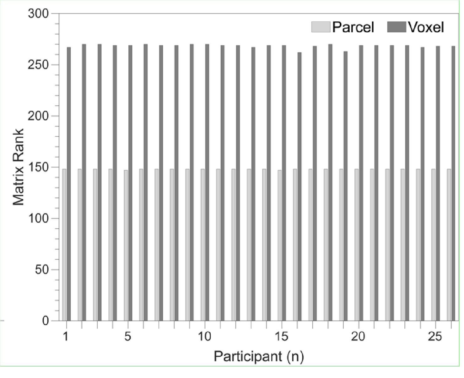
Figure 2—figure Supplement 2 in the revised manuscript now shows that the degree of dependence between the two spatial scales varies over the regional voxel-space. That is, some voxels within a given parcel correlate strongly with the time-series of the parcel they belong to, while others do not. This finding is consistent with a documented increase in correlational structure of neural activity across spatial scales that does not reflect perfect dependency or orthogonality [9]. Notably, the regional voxel-spaces included in the hybridspace decoder are significantly less correlated with the averaged parcel-space time-series than excluded voxels. We now point readers to this new figure in the results.
Taken together, these results indicate that the multi-scale information in the hybrid feature set is complimentary rather than orthogonal. This is consistent with the idea that hybridspace features better represent multi-scale temporospatial dynamics reported to be a fundamental characteristic of how the brain stores and adapts memories, and generates behavior across species [9].
Reviewer #2 (Public review):
Summary:
The current paper consists of two parts. The first part is the rigorous feature optimization of the MEG signal to decode individual finger identity performed in a sequence (4-1-3-2-4; 1~4 corresponds to little~index fingers of the left hand). By optimizing various parameters for the MEG signal, in terms of (i) reconstructed source activity in voxel- and parcel-level resolution and their combination, (ii) frequency bands, and (iii) time window relative to press onset for each finger movement, as well as the choice of decoders, the resultant "hybrid decoder" achieved extremely high decoding accuracy (~95%). This part seems driven almost by pure engineering interest in gaining as high decoding accuracy as possible.
In the second part of the paper, armed with the successful 'hybrid decoder,' the authors asked more scientific questions about how neural representation of individual finger movement that is embedded in a sequence, changes during a very early period of skill learning and whether and how such representational change can predict skill learning. They assessed the difference in MEG feature patterns between the first and the last press 4 in sequence 41324 at each training trial and found that the pattern differentiation progressively increased over the course of early learning trials. Additionally, they found that this pattern differentiation specifically occurred during the rest period rather than during the practice trial. With a significant correlation between the trial-by-trial profile of this pattern differentiation and that for accumulation of offline learning, the authors argue that such "contextualization" of finger movement in a sequence (e.g., what-where association) underlies the early improvement of sequential skill. This is an important and timely topic for the field of motor learning and beyond.
Strengths:
Each part has its own strength. For the first part, the use of temporally rich neural information (MEG signal) has a significant advantage over previous studies testing sequential representations using fMRI. This allowed the authors to examine the earliest period (= the first few minutes of training) of skill learning with finer temporal resolution. Through the optimization of MEG feature extraction, the current study achieved extremely high decoding accuracy (approx. 94%) compared to previous works. For the second part, the finding of the early "contextualization" of the finger movement in a sequence and its correlation to early (offline) skill improvement is interesting and important. The comparison between "online" and "offline" pattern distance is a neat idea.
Weaknesses:
Despite the strengths raised, the specific goal for each part of the current paper, i.e., achieving high decoding accuracy and answering the scientific question of early skill learning, seems not to harmonize with each other very well. In short, the current approach, which is solely optimized for achieving high decoding accuracy, does not provide enough support and interpretability for the paper's interesting scientific claim. This reminds me of the accuracy-explainability tradeoff in machine learning studies (e.g., Linardatos et al., 2020). More details follow.
There are a number of different neural processes occurring before and after a key press, such as planning of upcoming movement and ahead around premotor/parietal cortices, motor command generation in primary motor cortex, sensory feedback related processes in sensory cortices, and performance monitoring/evaluation around the prefrontal area. Some of these may show learning-dependent change and others may not.
In this paper, the focus as stated in the Introduction was to evaluate “the millisecond-level differentiation of discrete action representations during learning”, a proposal that first required the development of more accurate computational tools. Our first step, reported here, was to develop that tool. With that in hand, we then proceeded to test if neural representations differentiated during early skill learning. Our results showed they did. Addressing the question the Reviewer asks is part of exciting future work, now possible based on the results presented in this paper. We acknowledge this issue in the revised Discussion:
Discussion (Lines 428-434):
“In this study, classifiers were trained on MEG activity recorded during or immediately after each keypress, emphasizing neural representations related to action execution, memory consolidation and recall over those related to planning. An important direction for future research is determining whether separate decoders can be developed to distinguish the representations or networks separately supporting these processes. Ongoing work in our lab is addressing this question. The present accuracy results across varied decoding window durations and alignment with each keypress action support the feasibility of this approach (Figure 3—figure supplement 5).”
Given the use of whole-brain MEG features with a wide time window (up to ~200 ms after each key press) under the situation of 3~4 Hz (i.e., 250~330 ms press interval) typing speed, these different processes in different brain regions could have contributed to the expression of the "contextualization," making it difficult to interpret what really contributed to the "contextualization" and whether it is learning related. Critically, the majority of data used for decoder training has the chance of such potential overlap of signal, as the typing speed almost reached a plateau already at the end of the 11th trial and stayed until the 36th trial. Thus, the decoder could have relied on such overlapping features related to the future presses. If that is the case, a gradual increase in "contextualization" (pattern separation) during earlier trials makes sense, simply because the temporal overlap of the MEG feature was insufficient for the earlier trials due to slower typing speed. Several direct ways to address the above concern, at the cost of decoding accuracy to some degree, would be either using the shorter temporal window for the MEG feature or training the model with the early learning period data only (trials 1 through 11) to see if the main results are unaffected would be some example.
We now include additional analyses carried out with decoding time windows ranging from 50 to 250ms in duration, which have been added to the revised manuscript as follows:
Results (lines 258-261):
“The improved decoding accuracy is supported by greater differentiation in neural representations of the index finger keypresses performed at positions 1 and 5 of the sequence (Figure 4A), and by the trial-by-trial increase in 2-class decoding accuracy over early learning (Figure 4C) across different decoder window durations (Figure 4 – figure supplement 2).”
Results (lines 310-312):
“Offline contextualization strongly correlated with cumulative micro-offline gains (r = 0.903, R<sup>2</sup> = 0.816, p < 0.001; Figure 5 – figure supplement 1A, inset) across decoder window durations ranging from 50 to 250ms (Figure 5 – figure supplement 1B, C).“
Discussion (lines 382-385):
“This was further supported by the progressive differentiation of neural representations of the index finger keypress (Figure 4A) and by the robust trial-by trial increase in 2-class decoding accuracy across time windows ranging between 50 and 250ms (Figure 4C; Figure 4 – figure supplement 2).”
Discussion (lines 408-9):
“Offline contextualization consistently correlated with early learning gains across a range of decoding windows (50–250ms; Figure 5 – figure supplement 1).”
Several new control analyses are also provided addressing the question of overlapping keypresses:
Reviewer #3 (Public review):
Summary:
One goal of this paper is to introduce a new approach for highly accurate decoding of finger movements from human magnetoencephalography data via dimension reduction of a "multi-scale, hybrid" feature space. Following this decoding approach, the authors aim to show that early skill learning involves "contextualization" of the neural coding of individual movements, relative to their position in a sequence of consecutive movements.
Furthermore, they aim to show that this "contextualization" develops primarily during short rest periods interspersed with skill training and correlates with a performance metric which the authors interpret as an indicator of offline learning.
Strengths:
A strength of the paper is the innovative decoding approach, which achieves impressive decoding accuracies via dimension reduction of a "multi-scale, hybrid space". This hybridspace approach follows the neurobiologically plausible idea of concurrent distribution of neural coding across local circuits as well as large-scale networks. A further strength of the study is the large number of tested dimension reduction techniques and classifiers.
Weaknesses:
A clear weakness of the paper lies in the authors' conclusions regarding "contextualization". Several potential confounds, which partly arise from the experimental design (mainly the use of a single sequence) and which are described below, question the neurobiological implications proposed by the authors and provide a simpler explanation of the results. Furthermore, the paper follows the assumption that short breaks result in offline skill learning, while recent evidence, described below, casts doubt on this assumption.
Please, see below for detailed response to each of these points.
Specifically: The authors interpret the ordinal position information captured by their decoding approach as a reflection of neural coding dedicated to the local context of a movement (Figure 4). One way to dissociate ordinal position information from information about the moving effectors is to train a classifier on one sequence and test the classifier on other sequences that require the same movements, but in different positions (Kornysheva et al., Neuron 2019). In the present study, however, participants trained to repeat a single sequence (4-1-3-2-4).
A crucial difference between our present study and the elegant study from Kornysheva et al. (2019) in Neuron highlighted by the Reviewer is that while ours is a learning study, the Kornysheva et al. study is not. Kornysheva et al. included an initial separate behavioral training session (i.e. – performed outside of the MEG) during which participants learned associations between fractal image patterns and different keypress sequences. Then in a separate, later MEG session—after the stimulus-response associations had been already learned in the first session—participants were tasked with recalling the learned sequences in response to a presented visual cue (i.e. – the paired fractal pattern).
Our rationale for not including multiple sequences in the same Day 1 training session of our study design was that it would lead to prominent interference effects, as widely reported in the literature [10-12]. Thus, while we had to take the issue of interference into consideration for our design, the Kornysheva et al. study did not. While Kornysheva et al. aimed to “dissociate ordinal position information from information about the moving effectors”, we tested various untrained sequences on Day 2 allowing us to determine that the contextualization result was specific to the trained sequence. By using this approach, we avoided interference effects on the learning of the primary skill caused by simultaneous acquisition of a second skill.
The revised manuscript states our findings related to the Day 2 Control data in the following locations:
Results (lines 117-122):
“On the following day, participants were retested on performance of the same sequence (4-1-3-2-4) over 9 trials (Day 2 Retest), as well as on the single-trial performance of 9 different untrained control sequences (Day 2 Controls: 2-1-3-4-2, 4-2-4-3-1, 3-4-2-3-1, 1-4-3-4-2, 3-2-4-3-1, 1-4-2-3-1, 3-2-4-2-1, 3-2-1-4-2, and 4-23-1-4). As expected, an upward shift in performance of the trained sequence (0.68 ± SD 0.56 keypresses/s; t = 7.21, p < 0.001) was observed during Day 2 Retest, indicative of an overnight skill consolidation effect (Figure 1 – figure supplement 1A).”
Results (lines 212-219):
“Utilizing the highest performing decoders that included LDA-based manifold extraction, we assessed the robustness of hybrid-space decoding over multiple sessions by applying it to data collected on the following day during the Day 2 Retest (9-trial retest of the trained sequence) and Day 2 Control (single-trial performance of 9 different untrained sequences) blocks. The decoding accuracy for Day 2 MEG data remained high (87.11% ± SD 8.54% for the trained sequence during Retest, and 79.44% ± SD 5.54% for the untrained Control sequences; Figure 3 – figure supplement 4). Thus, index finger classifiers constructed using the hybrid decoding approach robustly generalized from Day 1 to Day 2 across trained and untrained keypress sequences.”
Results (lines 269-273):
“On Day 2, incorporating contextual information into the hybrid-space decoder enhanced classification accuracy for the trained sequence only (improving from 87.11% for 4-class to 90.22% for 5-class), while performing at or below-chance levels for the Control sequences (≤ 30.22% ± SD 0.44%). Thus, the accuracy improvements resulting from inclusion of contextual information in the decoding framework was specific for the trained skill sequence.”
As a result, ordinal position information is potentially confounded by the fixed finger transitions around each of the two critical positions (first and fifth press). Across consecutive correct sequences, the first keypress in a given sequence was always preceded by a movement of the index finger (=last movement of the preceding sequence), and followed by a little finger movement. The last keypress, on the other hand, was always preceded by a ring finger movement, and followed by an index finger movement (=first movement of the next sequence). Figure 4 - supplement 2 shows that finger identity can be decoded with high accuracy (>70%) across a large time window around the time of the keypress, up to at least +/-100 ms (and likely beyond, given that decoding accuracy is still high at the boundaries of the window depicted in that figure). This time window approaches the keypress transition times in this study. Given that distinct finger transitions characterized the first and fifth keypress, the classifier could thus rely on persistent (or "lingering") information from the preceding finger movement, and/or "preparatory" information about the subsequent finger movement, in order to dissociate the first and fifth keypress.
Currently, the manuscript provides little evidence that the context information captured by the decoding approach is more than a by-product of temporally extended, and therefore overlapping, but independent neural representations of consecutive keypresses that are executed in close temporal proximity - rather than a neural representation dedicated to context.
During the review process, the authors pointed out that a "mixing" of temporally overlapping information from consecutive keypresses, as described above, should result in systematic misclassifications and therefore be detectable in the confusion matrices in Figures 3C and 4B, which indeed do not provide any evidence that consecutive keypresses are systematically confused. However, such absence of evidence (of systematic misclassification) should be interpreted with caution, and, of course, provides no evidence of absence. The authors also pointed out that such "mixing" would hamper the discriminability of the two ordinal positions of the index finger, given that "ordinal position 5" is systematically followed by "ordinal position 1". This is a valid point which, however, cannot rule out that "contextualization" nevertheless reflects the described "mixing".
The revised manuscript contains several control analyses which rule out this potential confound.
Results (lines 318-328):
“Within-subject correlations were consistent with these group-level findings. The average correlation between offline contextualization and micro-offline gains within individuals was significantly greater than zero (Figure 5 – figure supplement 4, left; t = 3.87, p = 0.00035, df = 25, Cohen's d = 0.76) and stronger than correlations between online contextualization and either micro-online (Figure 5 – figure supplement 4, middle; t = 3.28, p = 0.0015, df = 25, Cohen's d = 1.2) or micro-offline gains (Figure 5 – figure supplement 4, right; t = 3.7021, p = 5.3013e-04, df = 25, Cohen's d = 0.69). These findings were not explained by behavioral changes of typing rhythm (t = -0.03, p = 0.976; Figure 5 – figure supplement 5), adjacent keypress transition times (R<sup>2</sup> = 0.00507, F[1,3202] = 16.3; Figure 5 – figure supplement 6), or overall typing speed (between-subject; R<sup>2</sup> = 0.028, p \= 0.41; Figure 5 – figure supplement 7).”
Results (lines 385-390):
“Further, the 5-class classifier—which directly incorporated information about the sequence location context of each keypress into the decoding pipeline—improved decoding accuracy relative to the 4-class classifier (Figure 4C). Importantly, testing on Day 2 revealed specificity of this representational differentiation for the trained skill but not for the same keypresses performed during various unpracticed control sequences (Figure 5C).”
Discussion (lines 408-423):
“Offline contextualization consistently correlated with early learning gains across a range of decoding windows (50–250ms; Figure 5 – figure supplement 1). This result remained unchanged when measuring offline contextualization between the last and second sequence of consecutive trials, inconsistent with a possible confounding effect of pre-planning [30] (Figure 5 – figure supplement 2A). On the other hand, online contextualization did not predict learning (Figure 5 – figure supplement 3). Consistent with these results the average within-subject correlation between offline contextualization and micro-offline gains was significantly stronger than within subject correlations between online contextualization and either micro-online or micro-offline gains (Figure 5 – figure supplement 4).
Offline contextualization was not driven by trial-by-trial behavioral differences, including typing rhythm (Figure 5 – figure supplement 5) and adjacent keypress transition times (Figure 5 – figure supplement 6) nor by between-subject differences in overall typing speed (Figure 5 – figure supplement 7)—ruling out a reliance on differences in the temporal overlap of keypresses. Importantly, offline contextualization documented on Day 1 stabilized once a performance plateau was reached (trials 11-36), and was retained on Day 2, documenting overnight consolidation of the differentiated neural representations.”
During the review process, the authors responded to my concern that training of a single sequence introduces the potential confound of "mixing" described above, which could have been avoided by training on several sequences, as in Kornysheva et al. (Neuron 2019), by arguing that Day 2 in their study did include control sequences. However, the authors' findings regarding these control sequences are fundamentally different from the findings in Kornysheva et al. (2019), and do not provide any indication of effector-independent ordinal information in the described contextualization - but, actually, the contrary. In Kornysheva et al. (Neuron 2019), ordinal, or positional, information refers purely to the rank of a movement in a sequence. In line with the idea of competitive queuing, Kornysheva et al. (2019) have shown that humans prepare for a motor sequence via a simultaneous representation of several of the upcoming movements, weighted by their rank in the sequence. Importantly, they could show that this gradient carries information that is largely devoid of information about the order of specific effectors involved in a sequence, or their timing, in line with competitive queuing. They showed this by training a classifier to discriminate between the five consecutive movements that constituted one specific sequence of finger movements (five classes: 1st, 2nd, 3rd, 4th, 5th movement in the sequence) and then testing whether that classifier could identify the rank (1st, 2nd, 3rd, etc) of movements in another sequence, in which the fingers moved in a different order, and with different timings. Importantly, this approach demonstrated that the graded representations observed during preparation were largely maintained after this cross decoding, indicating that the sequence was represented via ordinal position information that was largely devoid of information about the specific effectors or timings involved in sequence execution. This result differs completely from the findings in the current manuscript. Dash et al. report a drop in detected ordinal position information (degree of contextualization in figure 5C) when testing for contextualization in their novel, untrained sequences on Day 2, indicating that context and ordinal information as defined in Dash et al. is not at all devoid of information about the specific effectors involved in a sequence. In this regard, a main concern in my public review, as well as the second reviewer's public review, is that Dash et al. cannot tell apart, by design, whether there is truly contextualization in the neural representation of a sequence (which they claim), or whether their results regarding "contextualization" are explained by what they call "mixing" in their author response, i.e., an overlap of representations of consecutive movements, as suggested as an alternative explanation by Reviewer 2 and myself.
Again, as stated in response to a related comment by the Reviewer above, it is not surprising that our results differ from the study by Kornysheva et al. (2019) . A crucial difference between the studies that the Reviewer fails to recognize is that while ours is a learning study, the Kornysheva et al. study is not. Our rationale for not including multiple sequences in the same Day 1 training session of our study design was that it would lead to prominent interference effects, as widely reported in the literature [10-12]. Thus, while we had to take the issue of interference into consideration for our design, the Kornysheva et al. study did not, since it was not concerned with learning dynamics. The strengths of the elegant Kornysheva study highlighted by the Reviewer—that the pre-planned sequence queuing gradient of sequence actions was independent of the effectors or timings used—is precisely due to the fact that participants were selecting between sequence options that had been previously—and equivalently—learned. The decoders in the Kornynsheva study were trained to classify effector- and timing-independent sequence position information— by design—so it is not surprising that this is the information they reflect.
The questions asked in our study were different: 1) Do the neural representations of the same sequence action executed in different skill (ordinal sequence) locations differentiate (contextualize) during early learning? and 2) Is the observed contextualization specific to the learned sequence? Thus, while Kornysheva et al. aimed to “dissociate ordinal position information from information about the moving effectors”, we tested various untrained sequences on Day 2 allowing us to determine that the contextualization result was specific to the trained sequence. By using this approach, we avoided interference effects on the learning of the primary skill caused by simultaneous acquisition of a second skill.
Such temporal overlap of consecutive, independent finger representations may also account for the dynamics of "ordinal coding"/"contextualization", i.e., the increase in 2class decoding accuracy, across Day 1 (Figure 4C). As learning progresses, both tapping speed and the consistency of keypress transition times increase (Figure 1), i.e., consecutive keypresses are closer in time, and more consistently so. As a result, information related to a given keypress is increasingly overlapping in time with information related to the preceding and subsequent keypresses. The authors seem to argue that their regression analysis in Figure 5 - figure supplement 3 speaks against any influence of tapping speed on "ordinal coding" (even though that argument is not made explicitly in the manuscript). However, Figure 5 - figure supplement 3 shows inter-individual differences in a between-subject analysis (across trials, as in panel A, or separately for each trial, as in panel B), and, therefore, says little about the within-subject dynamics of "ordinal coding" across the experiment. A regression of trial-by-trial "ordinal coding" on trial-by-trial tapping speed (either within-subject, or at a group-level, after averaging across subjects) could address this issue. Given the highly similar dynamics of "ordinal coding" on the one hand (Figure 4C), and tapping speed on the other hand (Figure 1B), I would expect a strong relationship between the two in the suggested within-subject (or group-level) regression.
The aim of the between-subject regression analysis presented in the Results (see below) and in Figure 5—figure supplement 7 (previously Figure 5—figure supplement 3) of the revised manuscript, was to rule out a general effect of tapping speed on the magnitude of contextualization observed. If temporal overlap of neural representations was driving their differentiation, then participants typing at higher speeds should also show greater contextualization scores. We made the decision to use a between-subject analysis to address this issue since within-subject skill speed variance was rather small over most of the training session.
The Reviewer’s request that we additionally carry-out a “regression of trial-by-trial "ordinal coding" on trial-by-trial tapping speed (either within-subject, or at a group-level, after averaging across subjects)” is essentially the same request of Reviewer 2 above. That request was to perform a modified simple linear regression analysis where the predictor is the sum the 4-4 and 4-1 transition times, since these transitions are where any temporal overlaps of neural representations would occur. A new Figure 5 – figure supplement 6 in the revised manuscript includes a scatter plot showing the sum of adjacent index finger keypress transition times (i.e. – the 4-4 transition at the conclusion of one sequence iteration and the 4-1 transition at the beginning of the next sequence iteration) versus online contextualization distances measured during practice trials. Both the keypress transition times and online contextualization scores were z-score normalized within individual subjects, and then concatenated into a single data superset. As is clear in the figure data, results of the regression analysis showed a very weak linear relationship between the two (R<sup>2</sup> = 0.00507, F[1,3202] = 16.3). Thus, contextualization score magnitudes do not reflect the amount of overlap between adjacent keypresses when assessed either within- or between-subject.
The revised manuscript now states:
Results (lines 318-328):
“Within-subject correlations were consistent with these group-level findings. The average correlation between offline contextualization and micro-offline gains within individuals was significantly greater than zero (Figure 5 – figure supplement 4, left; t = 3.87, p = 0.00035, df = 25, Cohen's d = 0.76) and stronger than correlations between online contextualization and either micro-online (Figure 5 – figure supplement 4, middle; t = 3.28, p = 0.0015, df = 25, Cohen's d = 1.2) or micro-offline gains (Figure 5 – figure supplement 4, right; t = 3.7021, p = 5.3013e-04, df = 25, Cohen's d = 0.69). These findings were not explained by behavioral changes of typing rhythm (t = -0.03, p = 0.976; Figure 5 – figure supplement 5), adjacent keypress transition times (R<sup>2</sup> = 0.00507, F[1,3202] = 16.3; Figure 5 – figure supplement 6), or overall typing speed (between-subject; R<sup>2</sup> = 0.028, p \= 0.41; Figure 5 – figure supplement 7).”
Furthermore, learning should increase the number of (consecutively) correct sequences, and, thus, the consistency of finger transitions. Therefore, the increase in 2-class decoding accuracy may simply reflect an increasing overlap in time of increasingly consistent information from consecutive keypresses, which allows the classifier to dissociate the first and fifth keypress more reliably as learning progresses, simply based on the characteristic finger transitions associated with each. In other words, given that the physical context of a given keypress changes as learning progresses - keypresses move closer together in time and are more consistently correct - it seems problematic to conclude that the mental representation of that context changes. To draw that conclusion, the physical context should remain stable (or any changes to the physical context should be controlled for).
The revised manuscript now addresses specifically the question of mixing of temporally overlapping information:
Results (Lines 310-328)
“Offline contextualization strongly correlated with cumulative micro-offline gains (r = 0.903, R<sup>2</sup> = 0.816, p < 0.001; Figure 5 – figure supplement 1A, inset) across decoder window durations ranging from 50 to 250ms (Figure 5 – figure supplement 1B, C). The offline contextualization between the final sequence of each trial and the second sequence of the subsequent trial (excluding the first sequence) yielded comparable results. This indicates that pre-planning at the start of each practice trial did not directly influence the offline contextualization measure [30] (Figure 5 – figure supplement 2A, 1st vs. 2nd Sequence approaches). Conversely, online contextualization (using either measurement approach) did not explain early online learning gains (i.e. – Figure 5 – figure supplement 3). Within-subject correlations were consistent with these group-level findings. The average correlation between offline contextualization and micro-offline gains within individuals was significantly greater than zero (Figure 5 – figure supplement 4, left; t = 3.87, p = 0.00035, df = 25, Cohen's d = 0.76) and stronger than correlations between online contextualization and either micro-online (Figure 5 – figure supplement 4, middle; t = 3.28, p = 0.0015, df = 25, Cohen's d = 1.2) or micro-offline gains (Figure 5 – figure supplement 4, right; t = 3.7021, p = 5.3013e-04, df = 25, Cohen's d = 0.69). These findings were not explained by behavioral changes of typing rhythm (t = -0.03, p = 0.976; Figure 5 – figure supplement 5), adjacent keypress transition times (R<sup>2</sup> = 0.00507, F[1,3202] = 16.3; Figure 5 – figure supplement 6), or overall typing speed (between-subject; R<sup>2</sup> = 0.028, p \= 0.41; Figure 5 – figure supplement 7). “
Discussion (Lines 417-423)
“Offline contextualization was not driven by trial-by-trial behavioral differences, including typing rhythm (Figure 5 – figure supplement 5) and adjacent keypress transition times (Figure 5 – figure supplement 6) nor by between-subject differences in overall typing speed (Figure 5 – figure supplement 7)—ruling out a reliance on differences in the temporal overlap of keypresses. Importantly, offline contextualization documented on Day 1 stabilized once a performance plateau was reached (trials 11-36), and was retained on Day 2, documenting overnight consolidation of the differentiated neural representations.”
A similar difference in physical context may explain why neural representation distances ("differentiation") differ between rest and practice (Figure 5). The authors define "offline differentiation" by comparing the hybrid space features of the last index finger movement of a trial (ordinal position 5) and the first index finger movement of the next trial (ordinal position 1). However, the latter is not only the first movement in the sequence but also the very first movement in that trial (at least in trials that started with a correct sequence), i.e., not preceded by any recent movement. In contrast, the last index finger of the last correct sequence in the preceding trial includes the characteristic finger transition from the fourth to the fifth movement. Thus, there is more overlapping information arising from the consistent, neighbouring keypresses for the last index finger movement, compared to the first index finger movement of the next trial. A strong difference (larger neural representation distance) between these two movements is, therefore, not surprising, given the task design, and this difference is also expected to increase with learning, given the increase in tapping speed, and the consequent stronger overlap in representations for consecutive keypresses. Furthermore, initiating a new sequence involves pre-planning, while ongoing practice relies on online planning (Ariani et al., eNeuro 2021), i.e., two mental operations that are dissociable at the level of neural representation (Ariani et al., bioRxiv 2023).
The revised manuscript now addresses specifically the question of pre-planning:
Results (lines 310-318):
“Offline contextualization strongly correlated with cumulative micro-offline gains (r = 0.903, R<sup>2</sup> = 0.816, p < 0.001; Figure 5 – figure supplement 1A, inset) across decoder window durations ranging from 50 to 250ms (Figure 5 – figure supplement 1B, C). The offline contextualization between the final sequence of each trial and the second sequence of the subsequent trial (excluding the first sequence) yielded comparable results. This indicates that pre-planning at the start of each practice trial did not directly influence the offline contextualization measure [30] (Figure 5 – figure supplement 2A, 1st vs. 2nd Sequence approaches). Conversely, online contextualization (using either measurement approach) did not explain early online learning gains (i.e. – Figure 5 – figure supplement 3).”
Discussion (lines 408-416):
“Offline contextualization consistently correlated with early learning gains across a range of decoding windows (50–250ms; Figure 5 – figure supplement 1). This result remained unchanged when measuring offline contextualization between the last and second sequence of consecutive trials, inconsistent with a possible confounding effect of pre-planning [30] (Figure 5 – figure supplement 2A). On the other hand, online contextualization did not predict learning (Figure 5 – figure supplement 3). Consistent with these results the average within-subject correlation between offline contextualization and micro-offline gains was significantly stronger than within-subject correlations between online contextualization and either micro-online or micro-offline gains (Figure 5 – figure supplement 4).”
A further complication in interpreting the results stems from the visual feedback that participants received during the task. Each keypress generated an asterisk shown above the string on the screen. It is not clear why the authors introduced this complicating visual feedback in their task, besides consistency with their previous studies. The resulting systematic link between the pattern of visual stimulation (the number of asterisks on the screen) and the ordinal position of a keypress makes the interpretation of "contextual information" that differentiates between ordinal positions difficult. During the review process, the authors reported a confusion matrix from a classification of asterisks position based on eye tracking data recorded during the task and concluded that the classifier performed at chance level and gaze was, thus, apparently not biased by the visual stimulation. However, the confusion matrix showed a huge bias that was difficult to interpret (a very strong tendency to predict one of the five asterisk positions, despite chance-level performance). Without including additional information for this analysis (or simply the gaze position as a function of the number of astersisk on the screen) in the manuscript, this important control analysis cannot be properly assessed, and is not available to the public.
We now include the gaze position data requested by the Reviewer alongside the confusion matrix results in Figure 4 – figure supplement 3.
Results (lines 207-211):
“An alternate decoder trained on ICA components labeled as movement or physiological artefacts (e.g. – head movement, ECG, eye movements and blinks; Figure 3 – figure supplement 3A, D) and removed from the original input feature set during the pre-processing stage approached chance-level performance (Figure 4 – figure supplement 3), indicating that the 4-class hybrid decoder results were not driven by task-related artefacts.” Results (lines 261-268):
“As expected, the 5-class hybrid-space decoder performance approached chance levels when tested with randomly shuffled keypress labels (18.41%± SD 7.4% for Day 1 data; Figure 4 – figure supplement 3C). Task-related eye movements did not explain these results since an alternate 5-class hybrid decoder constructed from three eye movement features (gaze position at the KeyDown event, gaze position 200ms later, and peak eye movement velocity within this window; Figure 4 – figure supplement 3A) performed at chance levels (cross-validated test accuracy = 0.2181; Figure 4 – figure supplement 3B, C). “
Discussion (Lines 362-368):
“Task-related movements—which also express in lower frequency ranges—did not explain these results given the near chance-level performance of alternative decoders trained on (a) artefact-related ICA components removed during MEG preprocessing (Figure 3 – figure supplement 3A-C) and on (b) task-related eye movement features (Figure 4 – figure supplement 3B, C). This explanation is also inconsistent with the minimal average head motion of 1.159 mm (± 1.077 SD) across the MEG recording (Figure 3 – figure supplement 3D).”
The rationale for the task design including the asterisks is presented below:
Methods (Lines 500-514)
“The five-item sequence was displayed on the computer screen for the duration of each practice round and participants were directed to fix their gaze on the sequence. Small asterisks were displayed above a sequence item after each successive keypress, signaling the participants' present position within the sequence. Inclusion of this feedback minimizes working memory loads during task performance [73]. Following the completion of a full sequence iteration, the asterisk returned to the first sequence item. The asterisk did not provide error feedback as it appeared for both correct and incorrect keypresses. At the end of each practice round, the displayed number sequence was replaced by a string of five "X" symbols displayed on the computer screen, which remained for the duration of the rest break. Participants were instructed to focus their gaze on the screen during this time. The behavior in this explicit, motor learning task consists of generative action sequences rather than sequences of stimulus-induced responses as in the serial reaction time task (SRTT). A similar real-world example would be manually inputting a long password into a secure online application in which one intrinsically generates the sequence from memory and receives similar feedback about the password sequence position (also provided as asterisks), which is typically ignored by the user.”
The authors report a significant correlation between "offline differentiation" and cumulative micro-offline gains. However, this does not address the question whether there is a trial-by-trial relation between the degree of "contextualization" and the amount of micro-offline gains - i.e., the question whether performance changes (micro-offline gains) are less pronounced across rest periods for which the change in "contextualization" is relatively low. The single-subject correlation between contextualization changes "during" rest and micro-offline gains (Figure 5 - figure supplement 4) addresses this question, however, the critical statistical test (are correlation coefficients significantly different from zero) is not included. Given the displayed distribution, it seems unlikely that correlation coefficients are significantly above zero.
As recommend by the Reviewer, we now include one-way right-tailed t-test results which provide further support to the previously reported finding. The mean of within-subject correlations between offline contextualization and cumulative micro-offline gains was significantly greater than zero (t = 3.87, p = 0.00035, df = 25, Cohen's d = 0.76; see Figure 5 – figure supplement 4, left), while correlations for online contextualization versus cumulative micro-online (t = -1.14, p = 0.8669, df = 25, Cohen's d = -0.22) or micro-offline gains t = -0.097, p = 0.5384, df = 25, Cohen's d = -0.019) were not. We have incorporated the significant one-way t-test for offline contextualization and cumulative micro-offline gains in the Results section of the revised manuscript (lines 313-318) and the Figure 5 – figure supplement 4 legend.
The authors follow the assumption that micro-offline gains reflect offline learning.
However, there is no compelling evidence in the literature, and no evidence in the present manuscript, that micro-offline gains (during any training phase) reflect offline learning. Instead, emerging evidence in the literature indicates that they do not (Das et al., bioRxiv 2024), and instead reflect transient performance benefits when participants train with breaks, compared to participants who train without breaks, however, these benefits vanish within seconds after training if both groups of participants perform under comparable conditions (Das et al., bioRxiv 2024). During the review process, the authors argued that differences in the design between Das et al. (2024) on the one hand (Experiments 1 and 2), and the study by Bönstrup et al. (2019) on the other hand, may have prevented Das et al. (2024) from finding the assumed (lasting) learning benefit by micro-offline consolidation. However, the Supplementary Material of Das et al. (2024) includes an experiment (Experiment S1) whose design closely follows the early learning phase of Bönstrup et al. (2019), and which, nevertheless, demonstrates that there is no lasting benefit of taking breaks for the acquired skill level, despite the presence of micro-offline gains.
We thank the Reviewer for alerting us to this new data added to the revised supplementary materials of Das et al. (2024) posted to bioRxiv. However, despite the Reviewer’s claim to the contrary, a careful comparison between the Das et al and Bönstrup et al studies reveal more substantive differences than similarities and does not “closely follows a large proportion of the early learning phase of Bönstrup et al. (2019)” as stated.
In the Das et al. Experiment S1, sixty-two participants were randomly assigned to “with breaks” or “no breaks” skill training groups. The “with breaks” group alternated 10 seconds of skill sequence practice with 10 seconds of rest over seven trials (2 min and 2 sec total training duration). This amounts to 66.7% of the early learning period defined by Bönstrup et al. (2019) (i.e. - eleven 10-second-long practice periods interleaved with ten 10-second-long rest breaks; 3 min 30 sec total training duration).
Also, please note that while no performance feedback nor reward was given in the Bönstrup et al. (2019) study, participants in the Das et al. study received explicit performance-based monetary rewards, a potentially crucial driver of differentiated behavior between the two studies:
“Participants were incentivized with bonus money based on the total number of correct sequences completed throughout the experiment.”
The “no breaks” group in the Das et al. study practiced the skill sequence for 70 continuous seconds. Both groups (despite one being labeled “no breaks”) follow training with a long 3-minute break (also note that since the “with breaks” group ends with 10 seconds of rest their break is actually longer), before finishing with a skill “test” over a continuous 50-second-long block. During the 70 seconds of training, the “with breaks” group shows more learning than the “no breaks” group. Interestingly, following the long 3minute break the “with breaks” group display a performance drop (relative to their performance at the end of training) that is stable over the full 50-second test, while the “no breaks” group shows an immediate performance improvement following the long break that continues to increase over the 50-second test.
Separately, there are important issues regarding the Das et al. study that should be considered through the lens of recent findings not referred to in the preprint. A major element of their experimental design is that both groups—“with breaks” and “no breaks”— actually receive quite a long 3-minute break just before the skill test. This long break is more than 2.5x the cumulative interleaved rest experienced by the “with breaks” group. Thus, although the design is intended to contrast the presence or absence of rest “breaks”, that difference between groups is no longer maintained at the point of the skill test.
The Das et al. results are most consistent with an alternative interpretation of the data— that the “no breaks” group experiences offline learning during their long 3-minute break. This is supported by the recent work of Griffin et al. (2025) where micro-array recordings from primary and premotor cortex were obtained from macaque monkeys while they performed blocks of ten continuous reaching sequences up to 81.4 seconds in duration (see source data for Extended Data Figure 1h) with 90 seconds of interleaved rest. Griffin et al. observed offline improvement in skill immediately following the rest break that was causally related to neural reactivations (i.e. – neural replay) that occurred during the rest break. Importantly, the highest density of reactivations was present in the very first 90second break between Blocks 1 and 2 (see Fig. 2f in Griffin et al., 2025). This supports the interpretation that both the “with breaks” and “no breaks” group express offline learning gains, with these gains being delayed in the “no breaks” group due to the practice schedule.
On the other hand, if offline learning can occur during this longer break, then why would the “with breaks” group show no benefit? Again, it could be that most of the offline gains for this group were front-loaded during the seven shorter 10-second rest breaks. Another possible, though not mutually exclusive, explanation is that the observed drop in performance in the “with breaks” group is driven by contextual interference. Specifically, similar to Experiments 1 and 2 in Das et al. (2024), the skill test is conducted under very different conditions than those which the “with breaks” group practiced the skill under (short bursts of practiced alternating with equally short breaks). On the other hand, the “no breaks” group is tested (50 seconds of continuous practice) under quite similar conditions to their training schedule (70 seconds of continuous practice). Thus, it is possible that this dissimilarity between training and test could lead to reduced performance in the “with breaks” group.
We made the following manuscript revisions related to these important issues:
Introduction (Lines 26-56)
“Practicing a new motor skill elicits rapid performance improvements (early learning) [1] that precede skill performance plateaus [5]. Skill gains during early learning accumulate over rest periods (micro-offline) interspersed with practice [1, 6-10], and are up to four times larger than offline performance improvements reported following overnight sleep [1]. During this initial interval of prominent learning, retroactive interference immediately following each practice interval reduces learning rates relative to interference after passage of time, consistent with stabilization of the motor memory [11]. Micro-offline gains observed during early learning are reproducible [7, 10-13] and are similar in magnitude even when practice periods are reduced by half to 5 seconds in length, thereby confirming that they are not merely a result of recovery from performance fatigue [11]. Additionally, they are unaffected by the random termination of practice periods, which eliminates the possibility of predictive motor slowing as a contributing factor [11]. Collectively, these behavioral findings point towards the interpretation that micro offline gains during early learning represent a form of memory consolidation [1].
This interpretation has been further supported by brain imaging and electrophysiological studies linking known memory-related networks and consolidation mechanisms to rapid offline performance improvements. In humans, the rate of hippocampo-neocortical neural replay predicts micro-offline gains [6]. Consistent with these findings, Chen et al. [12] and Sjøgård et al. [13] furnished direct evidence from intracranial human EEG studies, demonstrating a connection between the density of hippocampal sharp-wave ripples (80-120 Hz)—recognized markers of neural replay—and micro-offline gains during early learning. Further, Griffin et al. reported that neural replay of task-related ensembles in the motor cortex of macaques during brief rest periods— akin to those observed in humans [1, 6-8, 14]—are not merely correlated with, but are causal drivers of micro-offline learning [15]. Specifically, the same reach directions that were replayed the most during rest breaks showed the greatest reduction in path length (i.e. – more efficient movement path between two locations in the reach sequence) during subsequent trials, while stimulation applied during rest intervals preceding performance plateau reduced reactivation rates and virtually abolished micro-offline gains [15]. Thus, converging evidence in humans and non-human primates across indirect non-invasive and direct invasive recording techniques link hippocampal activity, neural replay dynamics and offline skill gains in early motor learning that precede performance plateau.”
Next, in the Methods, we articulate important constrains formulated by Pan and Rickard and Bonstrup et al for meaningful measurements:
Methods (Lines 493-499)
“The study design followed specific recommendations by Pan and Rickard (2015): 1) utilizing 10-second practice trials and 2) constraining analysis of micro-offline gains to early learning trials (where performance monotonically increases and 95% of overall performance gains occur) that precede the emergence of “scalloped” performance dynamics strongly linked to reactive inhibition effects ( [29, 72]). This is precisely the portion of the learning curve Pan and Rickard referred to when they stated “…rapid learning during that period masks any reactive inhibition effect” [29].”
We finally discuss the implications of neglecting some or all of these recommendations:
Discussion (Lines 444-452):
“Finally, caution should be exercised when extrapolating findings during early skill learning, a period of steep performance improvements, to findings reported after insufficient practice [67], post-plateau performance periods [68], or non-learning situations (e.g. performance of non-repeating keypress sequences in [67]) when reactive inhibition or contextual interference effects are prominent. Ultimately, it will be important to develop new paradigms allowing one to independently estimate the different coincident or antagonistic features (e.g. - memory consolidation, planning, working memory and reactive inhibition) contributing to micro-online and micro-offline gains during and after early skill learning within a unifying framework.”
Along these lines, the authors' claim, based on Bönstrup et al. 2020, that "retroactive interference immediately following practice periods reduces micro-offline learning", is not supported by that very reference. Citing Bönstrup et al. (2020), "Regarding early learning dynamics (trials 1-5), we found no differences in microscale learning parameters (micro online/offline) or total early learning between both interference groups." That is, contrary to Dash et al.'s current claim, Bönstrup et al. (2020) did not find any retroactive interference effect on the specific behavioral readout (micro-offline gains) that the authors assume to reflect consolidation.
Please, note that the Bönstrup et al. 2020 paper abstract states:
“Third, retroactive interference immediately after each practice period reduced the learning rate relative to interference after passage of time (N = 373), indicating stabilization of the motor memory at a microscale of several seconds.”
which is further supported by this statement in the Results:
“The model comprised three parameters representing the initial performance, maximum performance and learning rate (see Eq. 1, “Methods”, “Data Analysis” section). We then statistically compared the model parameters between the interference groups (Fig. 2d). The late interference group showed a higher learning rate compared with the early interference group (late: 0.26 ± 0.23, early: 2.15 ± 0.20, P=0.04). The effect size of the group difference was small to medium (Cohen’s d 0.15)[29]. Similar differences with a stronger rise in the learning curve of a late interference groups vs. an early interference group were found in a smaller sample collected in the lab environment (Supplementary Fig. 3).”
We have modified the statement in the revised manuscript to specify that the difference observed was between learning rates: Introduction (Lines 30-32)
“During this initial interval of prominent learning, retroactive interference immediately following each practice interval reduces learning rates relative to interference after passage of time, consistent with stabilization of the motor memory [11].”
The authors conclude that performance improves, and representation manifolds differentiate, "during" rest periods (see, e.g., abstract). However, micro-offline gains (as well as offline contextualization) are computed from data obtained during practice, not rest, and may, thus, just as well reflect a change that occurs "online", e.g., at the very onset of practice (like pre-planning) or throughout practice (like fatigue, or reactive inhibition).
The Reviewer raises again the issue of a potential confound of “pre-planning” on our contextualization measures as in the comment above:
“Furthermore, initiating a new sequence involves pre-planning, while ongoing practice relies on online planning (Ariani et al., eNeuro 2021), i.e., two mental operations that are dissociable at the level of neural representation (Ariani et al., bioRxiv 2023).”
The cited studies by Ariani et al. indicate that effects of pre-planning are likely to impact the first 3 keypresses of the initial sequence iteration in each trial. As stated in the response to this comment above, we conducted a control analysis of contextualization that ignores the first sequence iteration in each trial to partial out any potential preplanning effect. This control analyses yielded comparable results, indicating that preplanning is not a major driver of our reported contextualization effects. We now report this in the revised manuscript:
We also state in the Figure 1 legend (Lines 99-103) in the revised manuscript that preplanning has no effect on the behavioral measures of micro-offline and micro-online gains in our dataset:
The Reviewer also raises the issue of possible effects stemming from “fatigue” and “reactive inhibition” which inhibit performance and are indeed relevant to skill learning studies. We designed our task to specifically mitigate these effects. We now more clearly articulate this rationale in the description of the task design as well as the measurement constraints essential for minimizing their impact.
We also discuss the implications of fatigue and reactive inhibition effects in experimental designs that neglect to follow these recommendations formulated by Pan and Rickard in the Discussion section and propose how this issue can be better addressed in future investigations.
To summarize, the results of our study indicate that: (a) offline contextualization effects are not explained by pre-planning of the first action sequence iteration in each practice trial; and (b) the task design implemented in this study purposefully minimize any possible effects of reactive inhibition or fatigue. Circling back to the Reviewer’s proposal that “contextualization…may just as well reflect a change that occurs "online"”, we show in this paper direct empirical evidence that contextualization develops to a greater extent across rest periods rather than across practice trials, contrary to the Reviewer’s proposal.
That is, the definition of micro-offline gains (as well as offline contextualization) conflates online and "offline" processes. This becomes strikingly clear in the recent Nature paper by Griffin et al. (2025), who computed micro-offline gains as the difference in average performance across the first five sequences in a practice period (a block, in their terminology) and the last five sequences in the previous practice period. Averaging across sequences in this way minimises the chance to detect online performance changes and inflates changes in performance "offline". The problem that "online" gains (or contextualization) is actually computed from data entirely generated online, and therefore subject to processes that occur online, is inherent in the very definition of micro-online gains, whether, or not, they computed from averaged performance.
We would like to make it clear that the issue raised by the Reviewer with respect to averaging across sequences done in the Griffin et al. (2025) study does not impact our study in any way. The primary skill measure used in all analyses reported in our paper is not temporally averaged. We estimated instantaneous correct sequence speed over the entire trial. Once the first sequence iteration within a trial is completed, the speed estimate is then updated at the resolution of individual keypresses. All micro-online and -offline behavioral changes are measured as the difference in instantaneous speed at the beginning and end of individual practice trials.
Methods (lines 528-530):
“The instantaneous correct sequence speed was calculated as the inverse of the average KTT across a single correct sequence iteration and was updated for each correct keypress.”
The instantaneous speed measure used in our analyses, in fact, maximizes the likelihood of detecting changes in online performance, as the Reviewer indicates. Despite this optimally sensitive measurement of online changes, our findings remained robust, consistently converging on the same outcome across our original analyses and the multiple controls recommended by the reviewers. Notably, online contextualization changes are significantly weaker than offline contextualization in all comparisons with different measurement approaches.
Results (lines 302-309)
“The Euclidian distance between neural representations of Index<sub>OP1</sub> (i.e. - index finger keypress at ordinal position 1 of the sequence) and Index<sub>OP5</sub> (i.e. - index finger keypress at ordinal position 5 of the sequence) increased progressively during early learning (Figure 5A)—predominantly during rest intervals (offline contextualization) rather than during practice (online) (t = 4.84, p < 0.001, df = 25, Cohen's d = 1.2; Figure 5B; Figure 5 – figure supplement 1A). An alternative online contextualization determination equalling the time interval between online and offline comparisons (Trial-based; 10 seconds between Index<sub>OP1</sub> and Index<sub>OP5</sub> observations in both cases) rendered a similar result (Figure 5 – figure supplement 2B).
Results (lines 316-318)
“Conversely, online contextualization (using either measurement approach) did not explain early online learning gains (i.e. – Figure 5 – figure supplement 3).”
Results (lines 318-328)
“Within-subject correlations were consistent with these group-level findings. The average correlation between offline contextualization and micro-offline gains within individuals was significantly greater than zero (Figure 5 – figure supplement 4, left; t = 3.87, p = 0.00035, df = 25, Cohen's d = 0.76) and stronger than correlations between online contextualization and either micro-online (Figure 5 – figure supplement 4, middle; t = 3.28, p = 0.0015, df = 25, Cohen's d = 1.2) or microoffline gains (Figure 5 – figure supplement 4, right; t = 3.7021, p = 5.3013e-04, df = 25, Cohen's d = 0.69). These findings were not explained by behavioral changes of typing rhythm (t = -0.03, p = 0.976; Figure 5 – figure supplement 5), adjacent keypress transition times (R<sup>2</sup> = 0.00507, F[1,3202] = 16.3; Figure 5 – figure supplement 6), or overall typing speed (between-subject; R<sup>2</sup> = 0.028, p \= 0.41; Figure 5 – figure supplement 7).”
We disagree with the Reviewer’s statement that “the definition of micro-offline gains (as well as offline contextualization) conflates online and "offline" processes”. From a strictly behavioral point of view, it is obviously true that one can only measure skill (rather than the absence of it during rest) to determine how it changes over time. While skill changes surrounding rest are used to infer offline learning processes, recovery of skill decay following intense practice is used to infer “unmeasurable” recovery from fatigue or reactive inhibition. In other words, the alternative processes proposed by the Reviewer also rely on the same inferential reasoning.
Importantly, inferences can be validated through the identification of mechanisms. Our experiment constrained the study to evaluation of changes in neural representations of the same action in different contexts, while minimized the impact of mechanisms related to fatigue/reactive inhibition [13, 14]. In this way, we observed that behavioral gains and neural contextualization occurs to a greater extent over rest breaks rather than during practice trials and that offline contextualization changes strongly correlate with the offline behavioral gains, while online contextualization does not. This result was supported by the results of all control analyses recommended by the Reviewers. Specifically:
Methods (Lines 493-499)
“The study design followed specific recommendations by Pan and Rickard (2015): 1) utilizing 10-second practice trials and 2) constraining analysis of micro-offline gains to early learning trials (where performance monotonically increases and 95% of overall performance gains occur) that precede the emergence of “scalloped” performance dynamics strongly linked to reactive inhibition effects ( [29, 72]). This is precisely the portion of the learning curve Pan and Rickard referred to when they stated “…rapid learning during that period masks any reactive inhibition effect” [29].”
And Discussion (Lines 444-448):
“Finally, caution should be exercised when extrapolating findings during early skill learning, a period of steep performance improvements, to findings reported after insufficient practice [67], post-plateau performance periods [68], or non-learning situations (e.g. performance of non-repeating keypress sequences in [67]) when reactive inhibition or contextual interference effects are prominent.”
Next, we show that offline contextualization is greater than online contextualization and predicts offline behavioral gains across all measurement approaches, including all controls suggested by the Reviewer’s comments and recommendations.
Results (lines 302-318):
“The Euclidian distance between neural representations of Index<sub>OP1</sub> (i.e. - index finger keypress at ordinal position 1 of the sequence) and Index<sub>OP5</sub> (i.e. - index finger keypress at ordinal position 5 of the sequence) increased progressively during early learning (Figure 5A)—predominantly during rest intervals (offline contextualization) rather than during practice (online) (t = 4.84, p < 0.001, df = 25, Cohen's d = 1.2; Figure 5B; Figure 5 – figure supplement 1A). An alternative online contextualization determination equalling the time interval between online and offline comparisons (Trial-based; 10 seconds between Index<sub>OP1</sub> and Index<sub>OP5</sub> observations in both cases) rendered a similar result (Figure 5 – figure supplement 2B).
Offline contextualization strongly correlated with cumulative micro-offline gains (r = 0.903, R<sup>2</sup> = 0.816, p < 0.001; Figure 5 – figure supplement 1A, inset) across decoder window durations ranging from 50 to 250ms (Figure 5 – figure supplement 1B, C). The offline contextualization between the final sequence of each trial and the second sequence of the subsequent trial (excluding the first sequence) yielded comparable results. This indicates that pre-planning at the start of each practice trial did not directly influence the offline contextualization measure [30] (Figure 5 – figure supplement 2A, 1st vs. 2nd Sequence approaches). Conversely, online contextualization (using either measurement approach) did not explain early online learning gains (i.e. – Figure 5 – figure supplement 3).”
Results (lines 318-324)
“Within-subject correlations were consistent with these group-level findings. The average correlation between offline contextualization and micro-offline gains within individuals was significantly greater than zero (Figure 5 – figure supplement 4, left; t = 3.87, p = 0.00035, df = 25, Cohen's d = 0.76) and stronger than correlations between online contextualization and either micro-online (Figure 5 – figure supplement 4, middle; t = 3.28, p = 0.0015, df = 25, Cohen's d = 1.2) or microoffline gains (Figure 5 – figure supplement 4, right; t = 3.7021, p = 5.3013e-04, df = 25, Cohen's d = 0.69).”
Discussion (lines 408-416):
“Offline contextualization consistently correlated with early learning gains across a range of decoding windows (50–250ms; Figure 5 – figure supplement 1). This result remained unchanged when measuring offline contextualization between the last and second sequence of consecutive trials, inconsistent with a possible confounding effect of pre-planning [30] (Figure 5 – figure supplement 2A). On the other hand, online contextualization did not predict learning (Figure 5 – figure supplement 3). Consistent with these results the average within-subject correlation between offline contextualization and micro-offline gains was significantly stronger than within subject correlations between online contextualization and either micro-online or micro-offline gains (Figure 5 – figure supplement 4).”
We then show that offline contextualization is not explained by pre-planning of the first action sequence:
Results (lines 310-316):
“Offline contextualization strongly correlated with cumulative micro-offline gains (r = 0.903, R<sup>2</sup> = 0.816, p < 0.001; Figure 5 – figure supplement 1A, inset) across decoder window durations ranging from 50 to 250ms (Figure 5 – figure supplement 1B, C). The offline contextualization between the final sequence of each trial and the second sequence of the subsequent trial (excluding the first sequence) yielded comparable results. This indicates that pre-planning at the start of each practice trial did not directly influence the offline contextualization measure [30] (Figure 5 – figure supplement 2A, 1st vs. 2nd Sequence approaches).”
Discussion (lines 409-412):
“This result remained unchanged when measuring offline contextualization between the last and second sequence of consecutive trials, inconsistent with a possible confounding effect of pre-planning [30] (Figure 5 – figure supplement 2A).”
In summary, none of the presented evidence in this paper—including results of the multiple control analyses carried out in response to the Reviewers’ recommendations— supports the Reviewer’s position.
Please note that the micro-offline learning "inference" has extensive mechanistic support across species and neural recording techniques (see Introduction, lines 26-56). In contrast, the reactive inhibition "inference," which is the Reviewer's alternative interpretation, has no such support yet [15].
Introduction (Lines 26-56)
“Practicing a new motor skill elicits rapid performance improvements (early learning) [1] that precede skill performance plateaus [5]. Skill gains during early learning accumulate over rest periods (micro-offline) interspersed with practice [1, 6-10], and are up to four times larger than offline performance improvements reported following overnight sleep [1]. During this initial interval of prominent learning, retroactive interference immediately following each practice interval reduces learning rates relative to interference after passage of time, consistent with stabilization of the motor memory [11]. Micro-offline gains observed during early learning are reproducible [7, 10-13] and are similar in magnitude even when practice periods are reduced by half to 5 seconds in length, thereby confirming that they are not merely a result of recovery from performance fatigue [11]. Additionally, they are unaffected by the random termination of practice periods, which eliminates the possibility of predictive motor slowing as a contributing factor [11]. Collectively, these behavioral findings point towards the interpretation that microoffline gains during early learning represent a form of memory consolidation [1].
This interpretation has been further supported by brain imaging and electrophysiological studies linking known memory-related networks and consolidation mechanisms to rapid offline performance improvements. In humans, the rate of hippocampo-neocortical neural replay predicts micro-offline gains [6].
Consistent with these findings, Chen et al. [12] and Sjøgård et al. [13] furnished direct evidence from intracranial human EEG studies, demonstrating a connection between the density of hippocampal sharp-wave ripples (80-120 Hz)—recognized markers of neural replay—and micro-offline gains during early learning. Further, Griffin et al. reported that neural replay of task-related ensembles in the motor cortex of macaques during brief rest periods— akin to those observed in humans [1, 6-8, 14]—are not merely correlated with, but are causal drivers of micro-offline learning [15]. Specifically, the same reach directions that were replayed the most during rest breaks showed the greatest reduction in path length (i.e. – more efficient movement path between two locations in the reach sequence) during subsequent trials, while stimulation applied during rest intervals preceding performance plateau reduced reactivation rates and virtually abolished micro-offline gains [15]. Thus, converging evidence in humans and non-human primates across indirect non-invasive and direct invasive recording techniques link hippocampal activity, neural replay dynamics and offline skill gains in early motor learning that precede performance plateau.”
That said, absence of evidence, is not evidence of absence and for that reason we also state in the Discussion (lines 448-452):
A simple control analysis based on shuffled class labels could lend further support to the authors' complex decoding approach. As a control analysis that completely rules out any source of overfitting, the authors could test the decoder after shuffling class labels. Following such shuffling, decoding accuracies should drop to chance-level for all decoding approaches, including the optimized decoder. This would also provide an estimate of actual chance-level performance (which is informative over and beyond the theoretical chance level). During the review process, the authors reported this analysis to the reviewers. Given that readers may consider following the presented decoding approach in their own work, it would have been important to include that control analysis in the manuscript to convince readers of its validity.
As requested, the label-shuffling analysis was carried out for both 4- and 5-class decoders and is now reported in the revised manuscript.
Results (lines 204-207):
“Testing the keypress state (4-class) hybrid decoder performance on Day 1 after randomly shuffling keypress labels for held-out test data resulted in a performance drop approaching expected chance levels (22.12%± SD 9.1%; Figure 3 – figure supplement 3C).”
Results (lines 261-264):
“As expected, the 5-class hybrid-space decoder performance approached chance levels when tested with randomly shuffled keypress labels (18.41%± SD 7.4% for Day 1 data; Figure 4 – figure supplement 3C).”
Furthermore, the authors' approach to cortical parcellation raises questions regarding the information carried by varying dipole orientations within a parcel (which currently seems to be ignored?) and the implementation of the mean-flipping method (given that there are two dimensions - space and time - it is unclear what the authors refer to when they talk about the sign of the "average source", line 477).
The revised manuscript now provides a more detailed explanation of the parcellation, and sign-flipping procedures implemented:
Methods (lines 604-611):
“Source-space parcellation was carried out by averaging all voxel time-series located within distinct anatomical regions defined in the Desikan-Killiany Atlas [31]. Since source time-series estimated with beamforming approaches are inherently sign-ambiguous, a custom Matlab-based implementation of the mne.extract_label_time_course with “mean_flip” sign-flipping procedure in MNEPython [78] was applied prior to averaging to prevent within-parcel signal cancellation. All voxel time-series within each parcel were extracted and the timeseries sign was flipped at locations where the orientation difference was greater than 90° from the parcel mode. A mean time-series was then computed across all voxels within the parcel after sign-flipping.”
Recommendations for the authors:
Reviewer #1 (Recommendations for the authors):
Comments on the revision:
The authors have made large efforts to address all concerns raised. A couple of suggestions remain:
- formally show if and how movement artefacts may contribute to the signal and analysis; it seems that the authors have data to allow for such an analysis
We have implemented the requested control analyses addressing this issue. They are reported in: Results (lines 207-211 and 261-268), Discussion (Lines 362-368):
- formally show that the signals from the intra- and inter parcel spaces are orthogonal.
Please note that, despite the Reviewer’s statement above, we never claim in the manuscript that the parcel-space and regional voxel-space features show “complete independence”.
Furthermore, the machine learning-based decoding methods used in the present study do not require input feature orthogonality, but instead non-redundancy [7], which is a requirement satisfied by our data (see below and the new Figure 2 – figure supplement 2 in the revised manuscript). Finally, our results already show that the hybrid space decoder outperformed all other methods even after input features were fully orthogonalized with LDA or PCA dimensionality reduction procedures prior to the classification step (Figure 3 – figure supplement 2).
We also highlight several additional results that are informative regarding this issue. For example, if spatially overlapping parcel- and voxel-space time-series only provided redundant information, inclusion of both as input features should increase model overfitting to the training dataset and decrease overall cross-validated test accuracy [8]. In the present study however, we see the opposite effect on decoder performance. First, Figure 3 – figure supplements 1 & 2 clearly show that decoders constructed from hybrid-space features outperform the other input feature (sensor-, whole-brain parcel- and whole-brain voxel-) spaces in every case (e.g. – wideband, all narrowband frequency ranges, and even after the input space is fully orthogonalized through dimensionality reduction procedures prior to the decoding step). Furthermore, Figure 3 – figure supplement 6 shows that hybridspace decoder performance supers when parcel-time series that spatially overlap with the included regional voxel-spaces are removed from the input feature set. We state in the Discussion (lines 353-356)
“The observation of increased cross-validated test accuracy (as shown in Figure 3 – Figure Supplement 6) indicates that the spatially overlapping information in parcel- and voxel-space time-series in the hybrid decoder was complementary, rather than redundant [41].”
To gain insight into the complimentary information contributed by the two spatial scales to the hybrid-space decoder, we first independently computed the matrix rank for whole-brain parcel- and voxel-space input features for each participant (shown in Author response image 1). The results indicate that whole-brain parcel-space input features are full rank (rank = 148) for all participants (i.e. - MEG activity is orthogonal between all parcels). The matrix rank of voxelspace input features (rank = 267± 17 SD), exceeded the parcel-space rank for all participants and approached the number of useable MEG sensor channels (n = 272). Thus, voxel-space features provide both additional and complimentary information to representations at the parcel-space scale.
Figure 2—figure Supplement 2 in the revised manuscript now shows that the degree of dependence between the two spatial scales varies over the regional voxel-space. That is, some voxels within a given parcel correlate strongly with the time-series of the parcel they belong to, while others do not. This finding is consistent with a documented increase in correlational structure of neural activity across spatial scales that does not reflect perfect dependency or orthogonality [9]. Notably, the regional voxel-spaces included in the hybridspace decoder are significantly less correlated with the averaged parcel-space time-series than excluded voxels. We now point readers to this new figure in the results.
Taken together, these results indicate that the multi-scale information in the hybrid feature set is complimentary rather than orthogonal. This is consistent with the idea that hybridspace features better represent multi-scale temporospatial dynamics reported to be a fundamental characteristic of how the brain stores and adapts memories, and generates behavior across species [9].
Reviewer #2 (Recommendations for the authors):
I appreciate the authors' efforts in addressing the concerns I raised. The responses generally made sense to me. However, I had some trouble finding several corrections/additions that the authors claim they made in the revised manuscript:
"We addressed this question by conducting a new multivariate regression analysis to directly assess whether the neural representation distance score could be predicted by the 4-1, 2-4, and 4-4 keypress transition times observed for each complete correct sequence (both predictor and response variables were z-score normalized within-subject). The results of this analysis also affirmed that the possible alternative explanation that contextualization effects are simple reflections of increased mixing is not supported by the data (Adjusted R<sup>2</sup> = 0.00431; F = 5.62). We now include this new negative control analysis in the revised manuscript."
This approach is now reported in the manuscript in the Results (Lines 324-328 and Figure 5-Figure Supplement 6 legend.
"We strongly agree with the Reviewer that the issue of generalizability is extremely important and have added a new paragraph to the Discussion in the revised manuscript highlighting the strengths and weaknesses of our study with respect to this issue."
Discussion (Lines 436-441)
“One limitation of this study is that contextualization was investigated for only one finger movement (index finger or digit 4) embedded within a relatively short 5-item skill sequence. Determining if representational contextualization is exhibited across multiple finger movements embedded within for example longer sequences (e.g. – two index finger and two little finger keypresses performed within a short piece of piano music) will be an important extension to the present results.”
"We strongly agree with the Reviewer that any intended clinical application must carefully consider the specific input feature constraints dictated by the clinical cohort, and in turn impose appropriate and complimentary constraints on classifier parameters that may differ from the ones used in the present study. We now highlight this issue in the Discussion of the revised manuscript and relate our present findings to published clinical BCI work within this context."
Discussion (Lines 441-444)
“While a supervised manifold learning approach (LDA) was used here because it optimized hybrid-space decoder performance, unsupervised strategies (e.g. - PCA and MDS, which also substantially improved decoding accuracy in the present study; Figure 3 – figure supplement 2) are likely more suitable for real-time BCI applications.”
and
"The Reviewer makes a good point. We have now implemented the suggested normalization procedure in the analysis provided in the revised manuscript."
Results (lines 275-282)
“We used a Euclidian distance measure to evaluate the differentiation of the neural representation manifold of the same action (i.e. - an index-finger keypress) executed within different local sequence contexts (i.e. - ordinal position 1 vs. ordinal position 5; Figure 5). To make these distance measures comparable across participants, a new set of classifiers was then trained with group-optimal parameters (i.e. – broadband hybrid-space MEG data with subsequent manifold extraction (Figure 3 – figure supplements 2) and LDA classifiers (Figure 3 – figure supplements 7) trained on 200ms duration windows aligned to the KeyDown event (see Methods, Figure 3 – figure supplements 5). “
Where are they in the manuscript? Did I read the wrong version? It would be more helpful to specify with page/line numbers. Please also add the detailed procedure of the control/additional analyses in the Method.
As requested, we now refer to all manuscript revisions with specific line numbers. We have also included all detailed procedures related to any additional analyses requested by reviewers.
I also have a few other comments back to the authors' following responses:
"Thus, increased overlap between the "4" and "1" keypresses (at the start of the sequence) and "2" and "4" keypresses (at the end of the sequence) could artefactually increase contextualization distances even if the underlying neural representations for the individual keypresses remain unchanged. One must also keep in mind that since participants repeat the sequence multiple times within the same trial, a majority of the index finger keypresses are performed adjacent to one another (i.e. - the "4-4" transition marking the end of one sequence and the beginning of the next). Thus, increased overlap between consecutive index finger keypresses as typing speed increased should increase their similarity and mask contextualization- related changes to the underlying neural representations." "We also re-examined our previously reported classification results with respect to this issue.
We reasoned that if mixing effects reflecting the ordinal sequence structure is an important driver of the contextualization finding, these effects should be observable in the distribution of decoder misclassifications. For example, "4" keypresses would be more likely to be misclassified as "1" or "2" keypresses (or vice versa) than as "3" keypresses. The confusion matrices presented in Figures 3C and 4B and Figure 3-figure supplement 3A display a distribution of misclassifications that is inconsistent with an alternative mixing effect explanation of contextualization."
"Based upon the increased overlap between adjacent index finger keypresses (i.e. - "4-4" transition), we also reasoned that the decoder tasked with separating individual index finger keypresses into two distinct classes based upon sequence position, should show decreased performance as typing speed increases. However, Figure 4C in our manuscript shows that this is not the case. The 2-class hybrid classifier actually displays improved classification performance over early practice trials despite greater temporal overlap. Again, this is inconsistent with the idea that the contextualization effect simply reflects increased mixing of individual keypress features."
As the time window for MEG feature is defined after the onset of each press, it is more likely that the feature overlap is the current and the future presses, rather than the current and the past presses (of course the three will overlap at very fast typing speed). Therefore, for sequence 41324, if we note the planning-related processes by a Roman numeral, the overlapping features would be '4i', '1iii', '3ii', '2iv', and '4iv'. Assuming execution-related process (e.g., 1) and planning-related process (e.g., i) are not necessarily similar, especially in finer temporal resolution, the patterns for '4i' and '4iv' are well separated in terms of process 'i' and 'iv,' and this advantage will be larger in faster typing speed. This also applies to the other presses. Thus, the author's arguments about the masking of contextualization and misclassification due to pattern overlap seem odd. The most direct and probably easiest way to resolve this would be to use a shorter time window for the MEG feature. Some decrease in decoding accuracy in this case is totally acceptable for the science purpose.
The revised manuscript now includes analyses carried out with decoding time windows ranging from 50 to 250ms in duration. These additional results are now reported in:
Results (lines 258-268):
“The improved decoding accuracy is supported by greater differentiation in neural representations of the index finger keypresses performed at positions 1 and 5 of the sequence (Figure 4A), and by the trial-by-trial increase in 2-class decoding accuracy over early learning (Figure 4C) across different decoder window durations (Figure 4 – figure supplement 2). As expected, the 5-class hybrid-space decoder performance approached chance levels when tested with randomly shuffled keypress labels (18.41%± SD 7.4% for Day 1 data; Figure 4 – figure supplement 3C). Task-related eye movements did not explain these results since an alternate 5-class hybrid decoder constructed from three eye movement features (gaze position at the KeyDown event, gaze position 200ms later, and peak eye movement velocity within this window; Figure 4 – figure supplement 3A) performed at chance levels (crossvalidated test accuracy = 0.2181; Figure 4 – figure supplement 3B, C).”
Results (lines 310-316):
“Offline contextualization strongly correlated with cumulative micro-offline gains (r = 0.903, R² = 0.816, p < 0.001; Figure 5 – figure supplement 1A, inset) across decoder window durations ranging from 50 to 250ms (Figure 5 – figure supplement 1B, C). The offline contextualization between the final sequence of each trial and the second sequence of the subsequent trial (excluding the first sequence) yielded comparable results. This indicates that pre-planning at the start of each practice trial did not directly influence the offline contextualization measure [30] (Figure 5 – figure supplement 2A, 1st vs. 2nd Sequence approaches). “
Discussion (lines 380-385):
“The first hint of representational differentiation was the highest false-negative and lowest false-positive misclassification rates for index finger keypresses performed at different locations in the sequence compared with all other digits (Figure 3C). This was further supported by the progressive differentiation of neural representations of the index finger keypress (Figure 4A) and by the robust trial-by-trial increase in 2class decoding accuracy across time windows ranging between 50 and 250ms (Figure 4C; Figure 4 – figure supplement 2).”
Discussion (lines 408-9):
“Offline contextualization consistently correlated with early learning gains across a range of decoding windows (50–250ms; Figure 5 – figure supplement 1).”
"We addressed this question by conducting a new multivariate regression analysis to directly assess whether the neural representation distance score could be predicted by the 4-1, 2-4 and 4-4 keypress transition times observed for each complete correct sequence"
For regression analysis, I recommend to use total keypress time per a sequence (or sum of 4-1 and 4-4) instead of specific transition intervals, because there likely exist specific correlational structure across the transition intervals. Using correlated regressors may distort the result.
This approach is now reported in the manuscript:
Results (Lines 324-328) and Figure 5-Figure Supplement 6 legend.
"We do agree with the Reviewer that the naturalistic, generative, self-paced task employed in the present study results in overlapping brain processes related to planning, execution, evaluation and memory of the action sequence. We also agree that there are several tradeoffs to consider in the construction of the classifiers depending on the study aim. Given our aim of optimizing keypress decoder accuracy in the present study, the set of tradeoffs resulted in representations reflecting more the latter three processes, and less so the planning component. Whether separate decoders can be constructed to tease apart the representations or networks supporting these overlapping processes is an important future direction of research in this area. For example, work presently underway in our lab constrains the selection of windowing parameters in a manner that allows individual classifiers to be temporally linked to specific planning, execution, evaluation or memoryrelated processes to discern which brain networks are involved and how they adaptively reorganize with learning. Results from the present study (Figure 4-figure supplement 2) showing hybrid-space decoder prediction accuracies exceeding 74% for temporal windows spanning as little as 25ms and located up to 100ms prior to the KeyDown event strongly support the feasibility of such an approach."
I recommend that the authors add this paragraph or a paragraph like this to the Discussion. This perspective is very important and still missing in the revised manuscript.
We now included in the manuscript the following sections addressing this point:
Discussion (lines 334-338)
“The main findings of this study during which subjects engaged in a naturalistic, self-paced task were that individual sequence action representations differentiate during early skill learning in a manner reflecting the local sequence context in which they were performed, and that the degree of representational differentiation— particularly prominent over rest intervals—correlated with skill gains. “
Discussion (lines 428-434)
“In this study, classifiers were trained on MEG activity recorded during or immediately after each keypress, emphasizing neural representations related to action execution, memory consolidation and recall over those related to planning. An important direction for future research is determining whether separate decoders can be developed to distinguish the representations or networks separately supporting these processes. Ongoing work in our lab is addressing this question. The present accuracy results across varied decoding window durations and alignment with each keypress action support the feasibility of this approach (Figure 3—figure supplement 5).”
"The rapid initial skill gains that characterize early learning are followed by micro-scale fluctuations around skill plateau levels (i.e. following trial 11 in Figure 1B)" Is this a mention of Figure 1 Supplement 1 A?
The sentence was replaced with the following: Results (lines 108-110)
“Participants reached 95% of maximal skill (i.e. - Early Learning) within the initial 11 practice trials (Figure 1B), with improvements developing over inter-practice rest periods (micro-offline gains) accounting for almost all total learning across participants (Figure 1B, inset) [1].”
The citation below seems to have been selected by mistake;
"9. Chen, S. & Epps, J. Using task-induced pupil diameter and blink rate to infer cognitive load. Hum Comput Interact 29, 390-413 (2014)."
We thank the Reviewer for bringing this mistake to our attention. This citation has now been corrected.
Reviewer #3 (Recommendations for the authors):
The authors write in their response that "We now provide additional details in the Methods of the revised manuscript pertaining to the parcellation procedure and how the sign ambiguity problem was addressed in our analysis." I could not find anything along these lines in the (redlined) version of the manuscript and therefore did not change the corresponding comment in the public review.
The revised manuscript now provides a more detailed explanation of the parcellation, and sign-flipping procedure implemented:
Methods (lines 604-611):
“Source-space parcellation was carried out by averaging all voxel time-series located within distinct anatomical regions defined in the Desikan-Killiany Atlas [31]. Since source time-series estimated with beamforming approaches are inherently sign-ambiguous, a custom Matlab-based implementation of the mne.extract_label_time_course with “mean_flip” sign-flipping procedure in MNEPython [78] was applied prior to averaging to prevent within-parcel signal cancellation. All voxel time-series within each parcel were extracted and the timeseries sign was flipped at locations where the orientation difference was greater than 90° from the parcel mode. A mean time-series was then computed across all voxels within the parcel after sign-flipping.”
The control analysis based on a multivariate regression that assessed whether the neural representation distance score could be predicted by the 4-1, 2-4 and 4-4 keypress transition times, as briefly mentioned in the authors' responses to Reviewer 2 and myself, was not included in the manuscript and could not be sufficiently evaluated.
This approach is now reported in the manuscript: Results (Lines 324-328) and Figure 5-Figure Supplement 6 legend.
The authors argue that differences in the design between Das et al. (2024) on the one hand (Experiments 1 and 2), and the study by Bönstrup et al. (2019) on the other hand, may have prevented Das et al. (2024) from finding the assumed learning benefit by micro-offline consolidation. However, the Supplementary Material of Das et al. (2024) includes an experiment (Experiment S1) whose design closely follows a large proportion of the early learning phase of Bönstrup et al. (2019), and which, nevertheless, demonstrates that there is no lasting benefit of taking breaks with respect to the acquired skill level, despite the presence of micro-offline gains.
We thank the Reviewer for alerting us to this new data added to the revised supplementary materials of Das et al. (2024) posted to bioRxiv. However, despite the Reviewer’s claim to the contrary, a careful comparison between the Das et al and Bönstrup et al studies reveal more substantive differences than similarities and does not “closely follows a large proportion of the early learning phase of Bönstrup et al. (2019)” as stated.
In the Das et al. Experiment S1, sixty-two participants were randomly assigned to “with breaks” or “no breaks” skill training groups. The “with breaks” group alternated 10 seconds of skill sequence practice with 10 seconds of rest over seven trials (2 min and 2 sec total training duration). This amounts to 66.7% of the early learning period defined by Bönstrup et al. (2019) (i.e. - eleven 10-second long practice periods interleaved with ten 10-second long rest breaks; 3 min 30 sec total training duration). Also, please note that while no performance feedback nor reward was given in the Bönstrup et al. (2019) study, participants in the Das et al. study received explicit performance-based monetary rewards, a potentially crucial driver of differentiated behavior between the two studies:
“Participants were incentivized with bonus money based on the total number of correct sequences completed throughout the experiment.”
The “no breaks” group in the Das et al. study practiced the skill sequence for 70 continuous seconds. Both groups (despite one being labeled “no breaks”) follow training with a long 3-minute break (also note that since the “with breaks” group ends with 10 seconds of rest their break is actually longer), before finishing with a skill “test” over a continuous 50-second-long block. During the 70 seconds of training, the “with breaks” group shows more learning than the “no breaks” group. Interestingly, following the long 3minute break the “with breaks” group display a performance drop (relative to their performance at the end of training) that is stable over the full 50-second test, while the “no breaks” group shows an immediate performance improvement following the long break that continues to increase over the 50-second test.
Separately, there are important issues regarding the Das et al study that should be considered through the lens of recent findings not referred to in the preprint. A major element of their experimental design is that both groups—“with breaks” and “no breaks”— actually receive quite a long 3-minute break just before the skill test. This long break is more than 2.5x the cumulative interleaved rest experienced by the “with breaks” group. Thus, although the design is intended to contrast the presence or absence of rest “breaks”, that difference between groups is no longer maintained at the point of the skill test.
The Das et al results are most consistent with an alternative interpretation of the data— that the “no breaks” group experiences offline learning during their long 3-minute break. This is supported by the recent work of Griffin et al. (2025) where micro-array recordings from primary and premotor cortex were obtained from macaque monkeys while they performed blocks of ten continuous reaching sequences up to 81.4 seconds in duration (see source data for Extended Data Figure 1h) with 90 seconds of interleaved rest. Griffin et al. observed offline improvement in skill immediately following the rest break that was causally related to neural reactivations (i.e. – neural replay) that occurred during the rest break. Importantly, the highest density of reactivations was present in the very first 90second break between Blocks 1 and 2 (see Fig. 2f in Griffin et al., 2025). This supports the interpretation that both the “with breaks” and “no breaks” group express offline learning gains, with these gains being delayed in the “no breaks” group due to the practice schedule.
On the other hand, if offline learning can occur during this longer break, then why would the “with breaks” group show no benefit? Again, it could be that most of the offline gains for this group were front-loaded during the seven shorter 10-second rest breaks. Another possible, though not mutually exclusive, explanation is that the observed drop in performance in the “with breaks” group is driven by contextual interference. Specifically, similar to Experiments 1 and 2 in Das et al. (2024), the skill test is conducted under very different conditions than those which the “with breaks” group practiced the skill under (short bursts of practiced alternating with equally short breaks). On the other hand, the “no breaks” group is tested (50 seconds of continuous practice) under quite similar conditions to their training schedule (70 seconds of continuous practice). Thus, it is possible that this dissimilarity between training and test could lead to reduced performance in the “with breaks” group.
We made the following manuscript revisions related to these important issues:
Introduction (Lines 26-56)
“Practicing a new motor skill elicits rapid performance improvements (early learning) [1] that precede skill performance plateaus [5]. Skill gains during early learning accumulate over rest periods (micro-offline) interspersed with practice [1, 6-10], and are up to four times larger than offline performance improvements reported following overnight sleep [1]. During this initial interval of prominent learning, retroactive interference immediately following each practice interval reduces learning rates relative to interference after passage of time, consistent with stabilization of the motor memory [11]. Micro-offline gains observed during early learning are reproducible [7, 10-13] and are similar in magnitude even when practice periods are reduced by half to 5 seconds in length, thereby confirming that they are not merely a result of recovery from performance fatigue [11]. Additionally, they are unaffected by the random termination of practice periods, which eliminates the possibility of predictive motor slowing as a contributing factor [11]. Collectively, these behavioral findings point towards the interpretation that microoffline gains during early learning represent a form of memory consolidation [1].
This interpretation has been further supported by brain imaging and electrophysiological studies linking known memory-related networks and consolidation mechanisms to rapid offline performance improvements. In humans, the rate of hippocampo-neocortical neural replay predicts micro-offline gains [6]. Consistent with these findings, Chen et al. [12] and Sjøgård et al. [13] furnished direct evidence from intracranial human EEG studies, demonstrating a connection between the density of hippocampal sharp-wave ripples (80-120 Hz)—recognized markers of neural replay—and micro-offline gains during early learning. Further, Griffin et al. reported that neural replay of task-related ensembles in the motor cortex of macaques during brief rest periods— akin to those observed in humans [1, 6-8, 14]—are not merely correlated with, but are causal drivers of micro-offline learning [15]. Specifically, the same reach directions that were replayed the most during rest breaks showed the greatest reduction in path length (i.e. – more efficient movement path between two locations in the reach sequence) during subsequent trials, while stimulation applied during rest intervals preceding performance plateau reduced reactivation rates and virtually abolished micro-offline gains [15]. Thus, converging evidence in humans and non-human primates across indirect non-invasive and direct invasive recording techniques link hippocampal activity, neural replay dynamics and offline skill gains in early motor learning that precede performance plateau.”
Next, in the Methods, we articulate important constraints formulated by Pan and Rickard (2015) and Bönstrup et al. (2019) for meaningful measurements:
Methods (Lines 493-499)
“The study design followed specific recommendations by Pan and Rickard (2015): 1) utilizing 10-second practice trials and 2) constraining analysis of micro-offline gains to early learning trials (where performance monotonically increases and 95% of overall performance gains occur) that precede the emergence of “scalloped” performance dynamics strongly linked to reactive inhibition effects ([29, 72]). This is precisely the portion of the learning curve Pan and Rickard referred to when they stated “…rapid learning during that period masks any reactive inhibition effect” [29].”
We finally discuss the implications of neglecting some or all of these recommendations:
Discussion (Lines 444-452):
“Finally, caution should be exercised when extrapolating findings during early skill learning, a period of steep performance improvements, to findings reported after insufficient practice [67], post-plateau performance periods [68], or non-learning situations (e.g. performance of non-repeating keypress sequences in [67]) when reactive inhibition or contextual interference effects are prominent. Ultimately, it will be important to develop new paradigms allowing one to independently estimate the different coincident or antagonistic features (e.g. - memory consolidation, planning, working memory and reactive inhibition) contributing to micro-online and micro-offline gains during and after early skill learning within a unifying framework.”
Personally, given that the idea of (micro-offline) consolidation seems to attract a lot of interest (and therefore cause a lot of future effort/cost public money) in the scientific community, I would find it extremely important to be cautious in interpreting results in this field. For me, this would include abstaining from the claim that processes occur "during" a rest period (see abstract, for example), given that micro-offline gains (as well as offline contextualization) are computed from data obtained during practice, not rest, and may, thus, just as well reflect a change that occurs "online", e.g., at the very onset of practice (like pre-planning) or throughout practice (like fatigue, or reactive inhibition). In addition, I would suggest to discuss in more depth the actual evidence not only in favour, but also against, the assumption of micro-offline gains as a phenomenon of learning.
We agree with the reviewer that caution is warranted. Based upon these suggestions, we have now expanded the manuscript to very clearly define the experimental constraints under which different groups have successfully studied micro-offline learning and its mechanisms, the impact of fatigue/reactive inhibition on micro-offline performance changes unrelated to learning, as well as the interpretation problems that emerge when those recommendations are not followed.
We clearly articulate the crucial constrains recommended by Pan and Rickard (2015) and Bönstrup et al. (2019) for meaningful measurements and interpretation of offline gains in the revised manuscript.
Methods (Lines 493-499)
“The study design followed specific recommendations by Pan and Rickard (2015): 1) utilizing 10-second practice trials and 2) constraining analysis of micro-offline gains to early learning trials (where performance monotonically increases and 95% of overall performance gains occur) that precede the emergence of “scalloped” performance dynamics strongly linked to reactive inhibition effects ( [29, 72]). This is precisely the portion of the learning curve Pan and Rickard referred to when they stated “…rapid learning during that period masks any reactive inhibition effect” [29].”
In the Introduction, we review the extensive evidence emerging from LFP and microelectrode recordings in humans and monkeys (including causality of neural replay with respect to micro-offline gains and early learning in the Griffin et al. Nature 2025 publication):
Introduction (Lines 26-56)
“Practicing a new motor skill elicits rapid performance improvements (early learning) [1] that precede skill performance plateaus [5]. Skill gains during early learning accumulate over rest periods (micro-offline) interspersed with practice [1, 6-10], and are up to four times larger than offline performance improvements reported following overnight sleep [1]. During this initial interval of prominent learning, retroactive interference immediately following each practice interval reduces learning rates relative to interference after passage of time, consistent with stabilization of the motor memory [11]. Micro-offline gains observed during early learning are reproducible [7, 10-13] and are similar in magnitude even when practice periods are reduced by half to 5 seconds in length, thereby confirming that they are not merely a result of recovery from performance fatigue [11]. Additionally, they are unaffected by the random termination of practice periods, which eliminates the possibility of predictive motor slowing as a contributing factor [11]. Collectively, these behavioral findings point towards the interpretation that microoffline gains during early learning represent a form of memory consolidation [1].
This interpretation has been further supported by brain imaging and electrophysiological studies linking known memory-related networks and consolidation mechanisms to rapid offline performance improvements. In humans, the rate of hippocampo-neocortical neural replay predicts micro-offline gains [6]. Consistent with these findings, Chen et al. [12] and Sjøgård et al. [13] furnished direct evidence from intracranial human EEG studies, demonstrating a connection between the density of hippocampal sharp-wave ripples (80-120 Hz)—recognized markers of neural replay—and micro-offline gains during early learning. Further, Griffin et al. reported that neural replay of task-related ensembles in the motor cortex of macaques during brief rest periods— akin to those observed in humans [1, 6-8, 14]—are not merely correlated with, but are causal drivers of micro-offline learning [15]. Specifically, the same reach directions that were replayed the most during rest breaks showed the greatest reduction in path length (i.e. – more efficient movement path between two locations in the reach sequence) during subsequent trials, while stimulation applied during rest intervals preceding performance plateau reduced reactivation rates and virtually abolished micro-offline gains [15]. Thus, converging evidence in humans and non-human primates across indirect non-invasive and direct invasive recording techniques link hippocampal activity, neural replay dynamics and offline skill gains in early motor learning that precede performance plateau.”
Following the reviewer’s advice, we have expanded our discussion in the revised manuscript of alternative hypotheses put forward in the literature and call for caution when extrapolating results across studies with fundamental differences in design (e.g. – different practice and rest durations, or presence/absence of extrinsic reward, etc).
Discussion (Lines 444-452):
“Finally, caution should be exercised when extrapolating findings during early skill learning, a period of steep performance improvements, to findings reported after insufficient practice [67], post-plateau performance periods [68], or non-learning situations (e.g. performance of non-repeating keypress sequences in [67]) when reactive inhibition or contextual interference effects are prominent. Ultimately, it will be important to develop new paradigms allowing one to independently estimate the different coincident or antagonistic features (e.g. - memory consolidation, planning, working memory and reactive inhibition) contributing to micro-online and micro-offline gains during and after early skill learning within a unifying framework.”
References
(1) Zimerman, M., et al., Disrupting the Ipsilateral Motor Cortex Interferes with Training of a Complex Motor Task in Older Adults. Cereb Cortex, 2012.
(2) Waters, S., T. Wiestler, and J. Diedrichsen, Cooperation Not Competition: Bihemispheric tDCS and fMRI Show Role for Ipsilateral Hemisphere in Motor Learning. J Neurosci, 2017. 37(31): p. 7500-7512.
(3) Sawamura, D., et al., Acquisition of chopstick-operation skills with the nondominant hand and concomitant changes in brain activity. Sci Rep, 2019. 9(1): p. 20397.
(4) Lee, S.H., S.H. Jin, and J. An, The dieerence in cortical activation pattern for complex motor skills: A functional near- infrared spectroscopy study. Sci Rep, 2019. 9(1): p. 14066.
(5) Grafton, S.T., E. Hazeltine, and R.B. Ivry, Motor sequence learning with the nondominant left hand. A PET functional imaging study. Exp Brain Res, 2002. 146(3): p. 369-78.
(6) Buch, E.R., et al., Consolidation of human skill linked to waking hippocamponeocortical replay. Cell Rep, 2021. 35(10): p. 109193.
(7) Wang, L. and S. Jiang, A feature selection method via analysis of relevance, redundancy, and interaction, in Expert Systems with Applications, Elsevier, Editor. 2021.
(8) Yu, L. and H. Liu, Eeicient feature selection via analysis of relevance and redundancy. Journal of Machine Learning Research, 2004. 5: p. 1205-1224.
(9) Munn, B.R., et al., Multiscale organization of neuronal activity unifies scaledependent theories of brain function. Cell, 2024.
(10) Borragan, G., et al., Sleep and memory consolidation: motor performance and proactive interference eeects in sequence learning. Brain Cogn, 2015. 95: p. 54-61.
(11) Landry, S., C. Anderson, and R. Conduit, The eeects of sleep, wake activity and timeon-task on oeline motor sequence learning. Neurobiol Learn Mem, 2016. 127: p. 5663.
(12) Gabitov, E., et al., Susceptibility of consolidated procedural memory to interference is independent of its active task-based retrieval. PLoS One, 2019. 14(1): p. e0210876.
(13) Pan, S.C. and T.C. Rickard, Sleep and motor learning: Is there room for consolidation? Psychol Bull, 2015. 141(4): p. 812-34.
(14) , M., et al., A Rapid Form of Oeline Consolidation in Skill Learning. Curr Biol, 2019. 29(8): p. 1346-1351 e4.
(15) Gupta, M.W. and T.C. Rickard, Comparison of online, oeline, and hybrid hypotheses of motor sequence learning using a quantitative model that incorporate reactive inhibition. Sci Rep, 2024. 14(1): p. 4661.
Author response:
The following is the authors’ response to the previous reviews
Reviewer #1 (Public Review):
Summary:
This paper explores how diverse forms of inhibition impact firing rates in models for cortical circuits. In particular, the paper studies how the network operating point affects the balance of direct inhibition from SOM inhibitory neurons to pyramidal cells, and disinhibition from SOM inhibitory input to PV inhibitory neurons. This is an important issue as these two inhibitory pathways have largely been studies in isolation. Support for the main conclusions is generally solid, but could be strengthened by additional analyses.
Strengths
The paper has improved in revision, and the new intuitive summary statements added to the end of each results section are quite helpful. Weaknesses
The concern about whether the results hold outside of the range in which neural responses are linear remains. This is particularly true given the discontinuity observed in the stability measure. I appreciate the concern (provided in the response to the first round of reviews) that studying nonlinear networks requires a lot of work. A more limited undertaking would be to test the behavior of a spiking network at a few key points identified by your linearization approach. Such tests could use relatively simple (and perhaps imperfect) measures of gain and stability. This could substantially enhance the paper, regardless of the outcome.
We appreciate the reviewer’s concern and in our resubmission we explore if networks dynamics that operate outside of the case where linearization is possible would continue to show our main result on the (dis)entanglement of stability and gain; the short answer is yes. To this end we have added a new section and Figure to our main text.
“Gain and stability in stochastically forced E – PV – SOM circuits
To confirm that our results do not depend on our approach of a linearization around a fixed point, we numerically simulate similar networks as shown above (Figure 2) in which the E and PV population receive slow varying, large amplitude noise (Figure 6A). This leads to noisy rate dynamics sampling a large subspace of the full firing rate grid (r<sub>E</sub>,r<sub>P</sub>) and thus any linearization would fail to describe the network response. In this stochastically forced network we explore how adding an SOM modulation or a stimulus affects this subspace (Figure 6B). To quantify stability without linearization, we assume that a network is more stable the lower the mean and variance of E rates. This is because very stable networks can better quench input fluctuations [Kanashiro et al., 2017; Hennequin et al., 2018]. To quantify gain, we calculate the change in E rates when adding the stimulus, yet having identical noise realizations for stimulated and non-stimulated networks (Methods).
For the disinhibitory network without feedback a positive SOM modulation decreases stability due to increases of the mean and variance of E rates (Figure 6Ci) while the network gain increases (Figure 6Cii). As seen before (Figure 2A,B), stability and gain change in opposite directions in a disinhibitory circuit without feedback. Adding feedback PV → SOM and applying a negative SOM modulation increases both, stability and gain and therefore disentangles the inverse relation also in a noisy circuit (Figure 6D-F). This gives numerical support that our results do not depend on the assumption of linearization.
“Methods: Noisy input and numerical measurement of stability and gain
We consider a temporally smoothed input process ξ<sub>X</sub> with white noise ζ (zero mean, standard deviation one):  for populations X ∈{E,P} with timescale τ<sub>ξ</sub> = 50ms, σ<sub>X</sub> \= 6 and fixed mean input IX. To quantify the stability of the network without linearization, we assume that a network is more stable if the mean and variance of excitatory rates are low. To quantify network gain, we freeze the white noise process ζ for the case of with and without stimulus presentation and calculate the difference of E rates at each time point, leading to a distribution of network gains (Figure 6Cii,Fii). Total simulation time is 1000 seconds.”
We decided against using a spiking network because sufficiently asynchronous spiking network dynamics can still obey a linearized mean field theory (if the fluctuations in population firing rates are small). In our new analysis the firing rate deviations from the time averaged firing rate are sizable, making a linearization ineffective.
In summary, based on our additional analysis of recurrent circuits with noisy inputs we conclude that our results also hold in fluctuating networks, without the need of assuming realization aroud a stable fixed point.
Reviewer #2 (Public Review):
Summary:
Bos and colleagues address the important question of how two major inhibitory interneuron classes in the neocortex differentially affect cortical dynamics. They address this question by studying Wilson-Cowan-type mathematical models. Using a linearized fixed point approach, they provide convincing evidence that the existence of multiple interneuron classes can explain the counterintuitive finding that inhibitory modulation can increase the gain of the excitatory cell population while also increasing the stability of the circuit’s state to minor perturbations. This effect depends on the connection strengths within their circuit model, providing valuable guidance as to when and why it arises.
Overall, I find this study to have substantial merit. I have some suggestions on how to improve the clarity and completeness of the paper.
Strengths:
(1) The thorough investigation of how changes in the connectivity structure affect the gain-stability relationship is a major strength of this work. It provides an opportunity to understand when and why gain and stability will or will not both increase together. It also provides a nice bridge to the experimental literature, where different gain-stability relationships are reported from different studies.
(2) The simplified and abstracted mathematical model has the benefit of facilitating our understanding of this puzzling phenomenon. (I have some suggestions for how the authors could push this understanding further.) It is not easy to find the right balance between biologically-detailed models vs simple but mathematically tractable ones, and I think the authors struck an excellent balance in this study.
We thank the reviewer for their support of our work.
Weaknesses:
(1) The fixed-point analysis has potentially substantial limitations for understanding cortical computations away from the steady-state. I think the authors should have emphasized this limitation more strongly and possibly included some additional analyses to show that their conclusions extend to the chaotic dynamical regimes in which cortical circuits often live.
In the response to reviewer 1 we have included model analyses that addresses the limitations of linearization. Rather than use a chaotic model, which would require significant effort, we opted for a stochastically forced network, where the sizable fluctuations in rate dynamics preclude linearization.
(2) The authors could have discussed – even somewhat speculatively – how VIP interneurons fit into this picture. Their absence from this modelling framework stands out as a missed opportunity.
We agree that including VIP neurons into the framework would be an obvious and potentially interesting next step. At this point we only include them as potential modulators of SOM neurons. Modeling their dynamics without them receiving inputs from E, PV, or SOM neurons would be uninteresting. However, including them properly into the circuit would be outside the scope of the paper.
(3) The analysis is limited to paths within this simple E, PV, SOM circuit. This misses more extended paths (like thalamocortical loops) that involve interactions between multiple brain areas. Including those paths in the expansion in Eqs. 11-14 (Fig. 1C) may be an important consideration.
We agree that our pathway expansion can be used to study more than just the E – PV – SOM circuit. However, properly investigating full thalamocortcial loops should be done in a subsequent study.
Comments on revisions:
I think the authors have done a reasonable job of responding to my critiques, and the paper is in pretty good shape. (Also, thanks for correctly inferring that I meant VIP interneurons when I had written SST in my review! I have updated the public review accordingly.)
I still think this line of research would benefit substantially from considering dynamic regimes including chaotic ones. I strongly encourage the authors to consider such an extension in future work.
Please see our response above to Reviewer 1.
Reviewer #3 (Public Review):
Summary:
Bos et al study a computational model of cortical circuits with excitatory (E) and two subtypes of inhibition parvalbumin (PV) and somatostatin (SOM) expressing interneurons. They perform stability and gain analysis of simplified models with nonlinear transfer functions when SOM neurons are perturbed. Their analysis suggests that in a specific setup of connectivity, instability and gain can be untangled, such that SOM modulation leads to both increases in stability and gain, in contrast to the typical direction in neuronal networks where increased gain results in decreased stability.
Strengths:
- Analysis of the canonical circuit in response to SOM perturbations. Through numerical simulations and mathematical analysis, the authors have provided a rather comprehensive picture of how SOM modulation may affect response changes.
- Shedding light on two opposing circuit motifs involved in the canonical E-PV-SOM circuitry - namely, direct inhibition (SOM -¿ E) vs disinhibition (SOM -¿ PV -¿ E). These two pathways can lead to opposing effects, and it is often difficult to predict which one results from modulating SOM neurons. In simplified circuits, the authors show how these two motifs can emerge and depend on parameters like connection weights.
- Suggesting potentially interesting consequences for cortical computation. The authors suggest that certain regimes of connectivity may lead to untangling of stability and gain, such that increases in network gain are not compromised by decreasing stability. They also link SOM modulation in different connectivity regimes to versatile computations in visual processing in simple models.
We thank the reviewer for their support of our work.
Weaknesses
Computationally, the analysis is solid, but it’s very similar to previous studies (del Molino et al, 2017). Many studies in the past few years have done the perturbation analysis of a similar circuitry with or without nonlinear transfer functions (some of them listed in the references). This study applies the same framework to SOM perturbations, which is a useful computational analysis, in view of the complexity of the high-dimensional parameter space.
Link to biology: the most interesting result of the paper with regard to biology is the suggestion of a regime in which gain and stability can be modulated in an unconventional way - however, it is difficult to link the results to biological networks:
- A general weakness of the paper is a lack of direct comparison to biological parameters or experiments. How different experiments can be reconciled by the results obtained here, and what new circuit mechanisms can be revealed? In its current form, the paper reads as a general suggestion that different combinations of gain modulation and stability can be achieved in a circuit model equipped with many parameters (12 parameters). This is potentially interesting but not surprising, given the high dimensional space of possible dynamical properties. A more interesting result would have been to relate this to biology, by providing reasoning why it might be relevant to certain circuits (and not others), or to provide some predictions or postdictions, which are currently missing in the manuscript.
- For instance, a nice motivation for the paper at the beginning of the Results section is the different results of SOM modulation in different experiments - especially between L23 (inhibition) and L4 (disinhibition). But no further explanation is provided for why such a difference should exist, in view of their results and the insights obtained from their suggested circuit mechanisms. How the parameters identified for the two regimes correspond to different properties of different layers?
Please see our answer to the previous round of revision.
- One of the key assumptions of the model is nonlinear transfer functions for all neuron types. In terms of modelling and computational analysis, a thorough analysis of how and when this is necessary is missing (an analysis similar to what has been attempted in Figure 6 for synaptic weights, but for cellular gains). A discussion of this, along with the former analysis to know which nonlinearities would be necessary for the results, is needed, but currently missing from the study. The nonlinearity is assumed for all subtypes because it seems to be needed to obtain the results, but it’s not clear how the model would behave in the presence or absence of them, and whether they are relevant to biological networks with inhibitory transfer functions.
Please see our answer to the previous round of revision.
- Tuning curves are simulated for an individual orientation (same for all), not considering the heterogeneity of neuronal networks with multiple orientation selectivity (and other visual features) - making the model too simplistic.
Please see our answer to the previous round of revision.
Reviewer #1 (Recommendations For The Authors):
Introduction, first paragraph, last sentence: suggest ”sense,” -¿ ”sense” (no comma)
Introduction, second paragraph, first sentence: suggest ”is been” -¿ ”has been”
Introduction, very end of next to last paragraph: clarify ”modulate the circuit”
Figure 1 legend: can you make the ”Change ...” in the legend for 1D clearer - e.g. ”strenghen SOM → E connections and eliminate SOM → P connections”.
Paragraph immediately below Figure 1: In sentence starting ”Specifically ...” can you relate the cases described here back to the equation in Figure 1C?
Sentence right below equation 2: This sentence does not separate the network gain from the cellular gain as clearly as it could.
Page 7, second full paragraph: sentence starting ”Therefore, with ...” could be split into two or otherwise made clearer.
Sentence starting ”Furthermore” right below Figure 5 has an extra comma
We thank the reviewer for their additional comments, we made the respective changes in the manuscript.
Reviewer #3 (Recommendations For The Authors):
There is a long part in the reply letter discussing the link to biology - but the revised manuscript doesn’t seem to reflect that.
The information in the reply letter discussing the link to biology has been added at multiple points in the discussion. In the section ‘decision of labor between PV and SOM neurons’ we mention Ferguson and Carding 2020, in the section ‘impact of SOM neuron modulation on tuning curves’ we discuss Phillups and Hasenstaub 2016, and in the section ‘limitations and future directions’ we mention Tobin et al., 2023.
The writing can be improved - for example, see below instances:
P. 7: Intuitively, the inverse relationship follows for inhibitory and disinhibitory pathways (and their mixture) because the firing rate grid (heatmap) does not depend on how the SOM neurons inhibit the E - PV circuit.
P.8: We first remark that by adding feedback E connections onto SOM neurons, changes in SOM rates can now affect the underlying heatmaps in the (rE, rP) grid.
Not clear how ”rates can affect the heatmaps”. It’s too colloquial and not scientifically rigorous or sound.
We added further explanations at the respective places in the manuscript to improve the writing.
Author Response
The following is the authors’ response to the previous reviews.
We appreciate the constructive comments made by the editor and the reviewers. We have corrected errors and provided additional experimental data and analysis to address the latest criticisms raised by the reviewers and provided point-by-point response to the reviewers as below.
Reviewer #1 (Recommendations For The Authors):
I do acknowledge the work the authors put into this manuscript and I can accept the fact that the authors decided on a minimum of additional experiments. However, I would recommend the authors to be more concise by adding more information in the method and result sections about how they performed their experiments such as which Nav and AMPAR DNA constructs they used, the age of the mice, how long time they exposed the patches to quinidine, information on how many times they repeated their pull downs etc.
Answer: We thank the reviewer’s comments. we have incorporated the suggested modifications into our revised manuscript. Specifically, we have included detailed information on the NaV and AMPAR constructs in the Methods section. The age of the homozygous NaV1.6 knockout mice and the wild-type littermate controls is postnatal (P0-P1) (see in Results and Methods section). Prior to the application of step pulses, cells were subjected to the bath solution containing quinidine for approximately one minute (see in Methods section). Additionally, the co-immunoprecipitation assays for Slack and NaV1.6 were repeated three times (see in Methods section).
Minor detail in line 263: "...KCNT1 (Slack) have been identified to related to seizure..." I guess this should have been "...KCNT1 (Slack) have been identified and related to seizure..."?
Answer: We thank the reviewer for raising this point. We have corrected it in the revised manuscript.
Also, and again minor detail, I had a comment about the color coding in Fig 4 and by mistake, I added 4B, but I meant the use of colors in the entire figure, and mainly the use of colors in 4C, G and I.
Answer: We apologize for the confusion. We have changed the color coding of Figure 4 in the revised manuscript.
Reviewer #2 (Recommendations For The Authors):
While the paper is improved, several concerns do not seem to have been addressed. Some may have been missed because there is no response at all, but others may have been unclear because the response does not address the concern, but a related issue. Details are below.
Answer: We thank the reviewer for the criticisms. We have made changes of our manuscript to address the concerns.
Original issue:
3) Remove the term in vivo.
Answer: We thank the reviewer for raising this point. In our experiments, although we did not conduct experiments directly in living organisms, our results demonstrated the coimmunoprecipitation of NaV1.6 with Slack in homogenates from mouse cortical and hippocampal tissues (Fig. 3C). This result may support that the interaction between Slack and NaV1.6 occurs in vivo.
New comment from reviewer:
The argument to use the term in vivo is not well supported by what the authors have said. Just because tissues are used from an animal does not mean experiments were conducted in vivo. As the authors say, they did not conduct experiments in living organisms. Therefore the term in vivo should be avoided. This is a minor point.
Answer: We thank the reviewer for pointing this out. We have removed the term “in vivo” in the revised manuscript.
Original:
4) Figure 1C Why does Nav1.2 have a small inward current before the large inward current in the inset?
Answer: We apologize for the confusion. We would like to clarify that the small inward current can be attributed to the current of membrane capacitance (slow capacitance or C-slow). The larger inward current is mediated by NaV1.2.
New comment:
This is not well argued. Please note why the authors know the current is due to capacitance. Also, how do they know the larger current is due to NaV1.2? Please add that to the paper so readers know too.
Answer: We thank the reviewer’s comment. To provide a clearer representation of NaV1.2mediated currents in Fig. 1C, we have replaced the original example trace with a new one in which only one inward current is observed.
Original:
The slope of the rising phase of the larger sodium current seems greater than Nav1.6 or Nav1.5. Was this examined?
Answer: Additionally, we did not compare the slope of the rising phase of NaV subtypes sodium currents but primarily focused on the current amplitudes.
New comment:
This is not a strong answer. There seems to be an effect that the authors do not mention and evidently did not quantify that argues against their conclusion, which weakens the presentation.
Answer: We thank the reviewer’s comment. To assess the slope of the rising phase of NaV subtype currents, we compared the activation time constants of NaV1.2, NaV1.5, and NaV1.6 peak currents in HEK293 cells co-expressing NaV channel subtypes with Slack. The results have shown no significant differences (Author response image 1). We have included this analysis (see Fig. S9A) and the corresponding fitting equation (see in Methods section) in the revised manuscript.
Author response image 1.
The activation time constants of peak sodium currents in HEK293 cells co-expressing NaV1.2 (n=6), NaV1.5 (n=5), and NaV1.6 (n=5) with Slack, respectively. ns, p > 0.05, one-way ANOVA followed by Bonferroni’s post hoc test.
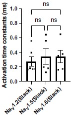
Original:
2D-E For Nav1.5 the sodium current is very large compared to Nav1.6. Is it possible the greater effect of quinidine for Nav1.6 is due to the lesser sodium current of Nav1.6?
Answer: We thank the reviewer for raising this point. We would like to clarify that our results indicate that transient sodium currents contribute to the sensitization of Slack to quinidine blockade (Fig. 2C,E). Therefore, it is unlikely that the greater effect observed for NaV1.6 in sensitizing Slack is due to its lower sodium currents.
New comment:
I am not sure the question I was asking was clear. How can the authors discount the possibility that quinidine is more effective on NaV1.6 because the NaV1.6 current is relatively weak?
Answer: We thank the reviewer for raising this point. We have examined the sodium current amplitudes of NaV1.5, NaV1.5/1.6 chimeras, and NaV1.6 upon co-expression of NaV with Slack. Our analysis revealed that there are no significant differences between NaV1.5 and NaV1.5/6N, with both exhibiting much larger current amplitudes compared to NaV1.6 (Author response image 2), but only NaV1.5/6N replicates the effect of NaV1.6 in sensitizing Slack to quinidine blockade (Fig. 4H-I), suggesting the observed differences between NaV1.5 and NaV1.6 in sensitizing Slack are unlikely to be attributed to NaV1.6's lower sodium currents but may instead involve NaV1.6's Nterminus-induced physical interaction. We have included this analysis in the revised manuscript (see Fig. S9B).
Author response image 2.
Comparison of peak sodium current amplitudes of NaV1.5 (n=9), NaV1.5/6NC (n=13), NaV1.5/6N (n=10), and NaV1.6 (n=8) upon co-expressed with Slack in HEK293 cells. ns, p > 0.05, * p < 0.05, ** p < 0.01, *** p < 0.001, **** p < 0.0001; one-way ANOVA followed by Bonferroni’s post hoc test.
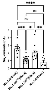
Original:
The differences between WT and KO in G -H are hard to appreciate. Could quantification be shown? The text uses words like "block" but this is not clear from the figure. It seems that the replacement of Na+ with Li+ did not block the outward current or effect of quinidine.
Answer: We apologize for the confusion. We would like to clarify the methods used in this experiment. The lithium ion (Li+) is a much weaker activator of sodium-activated potassium channel Slack than sodium ion (Na+)1,2.
Zhang Z, Rosenhouse-Dantsker A, Tang QY, Noskov S, Logothetis DE. The RCK2 domain uses a coordination site present in Kir channels to confer sodium sensitivity to Slo2.2 channels. J Neurosci. Jun 2 2010;30(22):7554-62. doi:10.1523/JNEUROSCI.0525-10.2010
Kaczmarek LK. Slack, Slick and Sodium-Activated Potassium Channels. ISRN Neurosci. Apr 18 2013;2013(2013)doi:10.1155/2013/354262 Therefore, we replaced Na+ with Li+ in the bath solution to measure the current amplitudes of sodium-activated potassium currents (IKNa)3.
Budelli G, Hage TA, Wei A, et al. Na+-activated K+ channels express a large delayed outward current in neurons during normal physiology. Nat Neurosci. Jun 2009;12(6):745-50. doi:10.1038/nn.2313
The following equation was used for quantification:
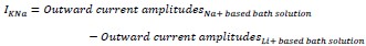
Furthermore, the remaining IKNa after application of 3 μM quinidine in the bath solution was measured as the following:
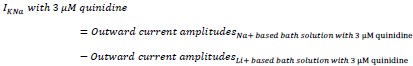
The quantification results were presented in Fig. 1K. The term "block" used in the text referred to the inhibitory effect of quinidine on IKNa.
New comment:
The fact remains that the term "block" is too strong for an effect that is incomplete. Also, the authors should add to the paper that Li+ is a weaker activator, so the reader knows some of the caveats to the approach.
Answer: We thank the reviewer for raising this point. We have added related citations and replaced the term “block” with “inhibit” in the revised manuscript.
Original:
- In K, for the WT, why is the effect of quinidine only striking for the largest currents?
Answer: We thank the reviewer for raising this point. After conducting an analysis, we found no correlation between the inhibitory effect of quinidine and the amplitudes of baseline IKNa in WT neurons (p = 0.6294) (Author response image 3). Therefore, the effect of quinidine is not solely limited to targeting the larger currents.
Author response image 3.
The correlation between the inhibitory effect of quinidine and the amplitudes of baseline IKNa in WT neurons (data from manuscript Fig. 1K). r = 0.1555, p=0.6294, Pearson correlation analysis.
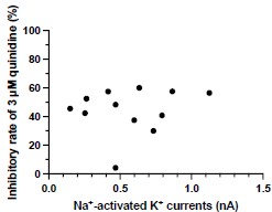
New comment:
Please add this to the paper and the figure as Supplemental.
Answer: We thank the reviewer for raising this point. We have added this figure as Fig.S3B in the revised manuscript.
Original:
5) Figure 2 A. The argument could be better made if the same concentration of quinidine were used for Slack and Slack + Nav1.6. It is recognized a greater sensitivity to quinidine is to be shown but as presented the figure is a bit confusing."
Answer: We apologize for the confusion. We would like to clarify that the presented concentrations of quinidine were chosen to be near the IC50 values for Slack and Slack+NaV1.6.
New comment:
Please add this to the paper.
Answer: We thank the reviewer for raising this point. We have added the clarification about the presented concentrations in the revised manuscript.
Original:
2C. Can the authors add the effect of quinidine to the condition where the prepulse potential was 90?"
Answer: We apologize for the confusion. We would like to clarify that the condition of prepulse potential at -90 mV is the same as the condition in Fig. 1. We only changed one experiment condition where the prepulse potential was changed to -40 mV from -90 mV.
New comment:
There was no confusion. The authors should consider adding the condition where the prepulse potential was -90.
Answer: We thank the reviewer for raising this point. We have added the clarification about the voltage condition in the revised manuscript (see in Fig. 2A caption).
Original:
2A. Clarify these 6 panels."
Answer: We thank the reviewer for raising this point. We have clarified the captions of Fig. 3A in the revised manuscript.
New comment: Clarification is needed. What is the blue? DAPI? What area of hippocamps? Please label cell layers. What area of cortex? Please label layers.
Answer: We thank the reviewer for raising this point. We have included the clarification in the Figure caption.
Original:
Figure 7. The images need more clarity. They are very hard to see. Text is also hard to see."
Answer: We apologize for the lack of clarity in the images and text. we would like to provide a concise summary of the key findings shown in this figure.
Figure 7 illustrates an innovative intervention for treating SlackG269S-induced seizures in mice by disrupting the Slack-NaV1.6 interaction. Our results showed that blocking NaV1.6-mediated sodium influx significantly reduced Slack current amplitudes (Fig. 2D,G), suggesting that the Slack-NaV1.6 interaction contributes to the current amplitudes of epilepsy-related Slack mutant variants, aggravating the gain-of-function phenotype. Additionally, Slack’s C-terminus is involved in the Slack-NaV1.6 interaction (Fig. 5D). We assumed that overexpressing Slack’s C-terminus can disrupt the Slack-NaV1.6 interaction (compete with Slack) and thereby encounter the current amplitudes of epilepsy-related Slack mutant variants.
In HEK293 cells, overexpression of Slack’s C-terminus indeed significantly reduced the current amplitudes of epilepsy-related SlackG288S and SlackR398Q upon co-expression with NaV1.5/6NC (Fig. 7A,B). Subsequently, we evaluated this intervention in an in vivo epilepsy model by introducing the Slack G269S variant into C57BL/6N mice using AAV injection, mimicking the human Slack mutation G288S that we previously identified (Fig. 7C-G).
New comment:
The images do not appear to have changed. Consider moving labels above the images so they can be distinguished better. Please label cell layers. Consider adding arrows to the point in the figure the authors want the reader to notice. The study design and timeline are unclear. What is (1) + (3), (2), etc.?
Answer: We thank the reviewer for pointing this out. We have modified Figure 7 in the revised manuscript and included the cell layer information in the Figure caption.
Original:
It is not clear how data were obtained because injection of kainic acid does not lead to a convulsive seizure every 10 min for several hours, which is what appears to be shown. Individual seizures are just at the beginning and then they merge at the start of status epilepticus. After the onset of status epilepticus the animals twitch, have varied movements, sometime rear and fall, but there is not a return to normal behavior. Therefore one can not call them individual seizures. In some strains of mice, however, individual convulsive seizures do occur (even if the EEG shows status epilepticus is occurring) but there are rarely more than 5 over several hours and the graph has many more. Please explain."
Answer: We apologize for the confusion. Regarding the data acquisition in relation to kainic acid injection, we initiated the timing following intraperitoneal injection of kainic acid and recorded the seizure scores of per mouse at ten-minute intervals, following the methodology described in previous studies4.
The seizure scores were determined using a modified Racine, Pinal, and Rovner scale5,6: (1) Facial movements; (2) head nodding; (3) forelimb clonus; (4) dorsal extension (rearing); (5) Loss of balance and falling; (6) Repeated rearing and failing; (7) Violent jumping and running; (8) Stage 7 with periods of tonus; (9) Dead.
Pinel JP, Rovner LI. Electrode placement and kindling-induced experimental epilepsy. Exp Neurol. Jan 15 1978;58(2):335-46. doi:10.1016/0014-4886(78)90145-0
Racine RJ. Modification of seizure activity by electrical stimulation. II. Motor seizure. Electroencephalogr Clin Neurophysiol. Mar 1972;32(3):281-94. doi:10.1016/00134694(72)90177-0
New comment:
This was clear. Perhaps my question was not clear. The question is how one can count individual seizures if animals have continuous seizures. It seems like the authors did not consider or observe status epilepticus but individual seizures. If that is true the data are hard to believe because too many seizures were counted. Animals do not have nearly this many seizures after kainic acid.
Answer: We appreciate the reviewer’s clarification. Our methodology involved assessing the maximum seizure scale during 10-minute intervals per mouse as previously described7, rather than counting individual seizures. For instance, a mouse exhibited the loss of balance and falling multiple times within 30-40 minute interval, we recorded the seizure scale as 5 for that time interval.
Reviewer #3 (Recommendations For The Authors):
While the authors have improved the manuscript, several outstanding issues still need to be addressed. Some may have been missed because there is no response at all, but others may have been unclear.
Answer: We thank the reviewer for the criticisms. We have added additional experimental data and analysis to address the concerns.
Original issue from Public Review:
- Immunolabeling of the hippocampus CA1 suggests sodium channels as well as Slack colocalization with AnkG (Fig 3A). Proximity ligation assay for NaV1.6 and Slack or a super-resolution microscopy approach would be needed to increase confidence in the presented colocalization results. Furthermore, coimmunoprecipitation studies on the membrane fraction would bolster the functional relevance of NaV1.6-Slack interaction on the cell surface.
Answer: We thank the reviewer for good suggestions. We acknowledge that employing proximity ligation assay and high-resolution techniques would significantly enhance our understanding of the localization of the Slack-NaV1.6 coupling.
At present, the technical capabilities available in our laboratory and institution do not support highresolution testing. However, we are enthusiastic about exploring potential collaborations to address these questions in the future. Furthermore, we fully recognize the importance of conducting coimmunoprecipitation (Co-IP) assays from membrane fractions. While we have already completed Co-IP assays for total protein and quantified the FRET efficiency values between Slack and NaV1.6 in the membrane region, the Co-IP assays on membrane fractions will be conducted in our future investigations.
New comment from reviewer: so far, the authors have not demonstrated that Nav1.6 and Slack interact on the cell surface.
Answer: We thank the reviewer for pointing this out. We acknowledgement that our data did not directly demonstrate interaction between NaV1.6 and Slack on the cell surface and we have removed related terminology in the revised manuscript. Notably, our patch-clamp experiments in Fig. 2D,G and Fig. S10B showed a Na+-mediated membrane current coupling of Slack and NaV1.6. Additionally, the FRET efficiency values between Slack and NaV1.6 were quantified in the membrane region. These findings suggest that membrane-near Slack interacts with NaV1.6.
- Although hippocampal slices from Scn8a+/- were used for studies in Fig. S8, it is not clear whether Scn8a-/- or Scn8a+/- tissue was used in other studies (Fig 1J & 1K). It will be important to clarify whether genetic manipulation of NaV1.6 expression (Fig. 1K) has an impact on sodiumactivated potassium current, level of surface Slack expression, or that of NaV1.6 near Slack.
Answer: We thank the reviewer for pointing this out. In Fig. 1G,J,K, primary cortical neurons from homozygous NaV1.6 knockout (Scn8a-/-) mice were used. We will clarify this information in the revised manuscript. In terms of the effects of genetic manipulation of NaV1.6 expression on IKNa and surface Slack expression, we compared the amplitudes of IKNa measured from homozygous NaV1.6 knockout (NaV1.6-KO) neurons and wild-type (WT) neurons. The results showed that homozygous knockout of NaV1.6 does not alter the amplitudes of IKNa (Author response image 4). The level of surface Slack expression will be tested further.
Author response image 4.
The amplitudes of IKNa in WT and NaV1.6-KO neurons (data from manuscript Fig. 1K). ns, p > 0.05, unpaired two-tailed Student’s t test.
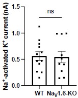
New comment from reviewer: The current version of the manuscrip>t does not contain these pertinent details and needs to be updated to include the information pertaining homozygous NaV1.6 knockouts. What age were these homozygous NaV1.6 knockout mice? These details need to be clearly stated in the manuscript.
Answer: We thank the reviewer for pointing this out. We have included this analysis in the revised manuscript (see Fig. S3A). The age of homozygous NaV1.6 knockout mice are P0-P1 and we have added this detail in the revised manuscript.
- Did the epilepsy-related Slack mutations have an impact on NaV1.6-mediated sodium current?
Answer: We thank the reviewer’s question. We examined the amplitudes of NaV1.6 sodium current upon expression alone or co-expression of NaV1.6 with epilepsy-related Slack mutations (K629N, R950Q, K985N). The results showed that the tested epilepsy-related Slack mutations do not alter the amplitudes of NaV1.6 sodium current (Author response image 5).
Author response image 5.
The amplitudes of NaV1.6 sodium currents upon co-expression of NaV1.6 with epilepsy-related Slack mutant variants (SlackK629N, SlackR950Q, and SlackK985N). ns, p>0.05, oneway ANOVA followed by Bonferroni’s post hoc test.
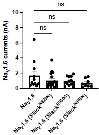
New comment from reviewer: Figure with the functional effect of co-expression of NaV1.6 with epilepsy-related Slack mutations should be included in the revised manuscript
Answer: We thank the reviewer for pointing this out. We have included this analysis in the revised manuscript (see Fig. S10A).
Original issue from Recommendations For The Authors:
- A reference to homozygous knockout is made in the abstract; however, only heterozygous mice are mentioned in the methods section. The genotype of the mice needs to be made clear in the manuscript. Furthermore, at what age were these mice used in the study. Since homozygous knockout of NaV1.6 is lethal at a very young age (<4 wks), it would be important to clarify that point as well.
Answer: We thank the reviewer for pointing this out. In the revised manuscript, we have included information about the source of the primary cortical neurons used in our study. These neurons were obtained from postnatal homozygous NaV1.6 knockout C3HeB/FeJ mice and their wild-type littermate controls.
New comment from reviewer: The answer that postnatal homozygous NaV1.6 knockout C3HeB/FeJ mice were used is insufficient. What age were these mice? This needs to be clearly stated in the manuscript.
Answer: We thank the reviewer for pointing this out. The postnatal homozygous NaV1.6 knockout C3HeB/FeJ mice and their wild-type littermate controls are in P0-P1. We have included this information in the revised manuscript.
- How long were the cells exposed to quinidine before the functional measurement were performed?
Answer: We thank the reviewer for pointing this out. The cells were exposed to the bath solution with quinidine for about one minute before applying step pulses.
New comment from reviewer: This needs to be clearly stated in the manuscript.
Answer: We thank the reviewer for pointing this out. We have included this information in the revised manuscript (see in Methods section).
- In Fig. 6B-D, it is not clear to what extent co-expression of Slack mutants and NaV1.6 increases sodium-activated potassium current.
Answer: We thank the reviewer for pointing this out. We notice that the current amplitudes of Slack mutants exhibit a considerable degree of variation, ranging from less than 1 nA to over 20 nA (n =58). To accurately measure the effects of NaV1.6 on increasing current amplitudes of Slack mutants, we plan to apply tetrodotoxin in the bath solution to block NaV1.6 sodium currents upon coexpression of Slack mutants with NaV1.6.
New comment from reviewer: Were these experiments with TTX completed? If so, they should be added to the revised manuscript.
Answer: We thank the reviewer for pointing this out. We compared the current amplitudes of epilepsy-related Slack mutant (SlackR950Q) before and after bath-application of 100 nM TTX upon co-expression with NaV1.6 in HEK293 cells. The results showed that bath-application of TTX significantly reduced the current amplitudes of SlackR950Q at +100 mV by nearly 40% (Author response image 6), suggesting NaV1.6 contributes to the current amplitudes of SlackR950Q. We have included this data in the revised manuscript (see Fig. S10B).
Author response image 6.
The current amplitudes of SlackR950Q before and after bath-application of 100 nM TTX upon co-expression with NaV1.6 in HEK293 cells (n=5). ***p < 0.001, Two-way repeated measures ANOVA followed by Bonferroni’s post hoc test.
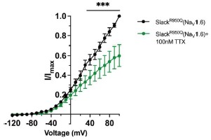
Additionally, we have corrected some errors in the methods and figure captions section:
Line 513, bath solution “5 glucose” should be “10 glucose.”
Figure 3A caption, the description “hippocampus CA1 (left) and neocortex (right)” was flipped and we have corrected it.
References
Zhang Z, Rosenhouse-Dantsker A, Tang QY, Noskov S, Logothetis DE. The RCK2 domain uses a coordination site present in Kir channels to confer sodium sensitivity to Slo2.2 channels. J Neurosci. Jun 2 2010;30(22):7554-62. doi:10.1523/JNEUROSCI.0525-10.2010
Kaczmarek LK. Slack, Slick and Sodium-Activated Potassium Channels. ISRN Neurosci. Apr 18 2013;2013(2013)doi:10.1155/2013/354262
Budelli G, Hage TA, Wei A, et al. Na+-activated K+ channels express a large delayed outward current in neurons during normal physiology. Nat Neurosci. Jun 2009;12(6):745-50. doi:10.1038/nn.2313
Huang Z, Walker MC, Shah MM. Loss of dendritic HCN1 subunits enhances cortical excitability and epileptogenesis. J Neurosci. Sep 2 2009;29(35):10979-88. doi:10.1523/JNEUROSCI.1531-09.2009
Pinel JP, Rovner LI. Electrode placement and kindling-induced experimental epilepsy. Exp Neurol. Jan 15 1978;58(2):335-46. doi:10.1016/0014-4886(78)90145-0
Racine RJ. Modification of seizure activity by electrical stimulation. II. Motor seizure. Electroencephalogr Clin Neurophysiol. Mar 1972;32(3):281-94. doi:10.1016/0013-4694(72)90177-0
Kim EC, Zhang J, Tang AY, et al. Spontaneous seizure and memory loss in mice expressing an epileptic encephalopathy variant in the calmodulin-binding domain of Kv7.2. Proc Natl Acad Sci U S A. Dec 21 2021;118(51)doi:10.1073/pnas.2021265118
Author response:
The following is the authors’ response to the previous reviews.
eLife assessment
In this important study, the authors report a novel measurement of the Escherichia coli chemotactic response and demonstrate that these bacteria display an attractant response to potassium, which is connected to intracellular pH level. Whilst the experiments are mostly convincing, there are some confounders regards pH changes and fluorescent proteins that remain to be addressed.
Public Reviews:
Reviewer #1 (Public Review):
Summary:
This paper shows that E. coli exhibits a chemotactic response to potassium by measuring both the motor response (using a bead assay) and the intracellular signaling response (CheY phosporylation level via FRET) to step changes in potassium concentration. They find increase in potassium concentration induces a considerable attractant response, with amplitude comparable to aspartate, and cells can quickly adapt (and generally over-adapt). The authors propose that the mechanism for potassium response is through modifying intracellular pH; they find both that potassium modifies pH and other pH modifiers induce similar attractant responses. It is also shown, using Tar- and Tsr-only mutants, that these two chemoreceptors respond to potassium differently. Tsr has a standard attractant response, while Tar has a biphasic response (repellent-like then attractant-like). Finally, the authors use computer simulations to study the swimming response of cells to a periodic potassium signal secreted from a biofilm and find a phase delay that depends on the period of oscillation.
Strengths:
The finding that E. coli can sense and adapt to potassium signals and the connection to intracellular pH is quite interesting and this work should stimulate future experimental and theoretical studies regarding the microscopic mechanisms governing this response. The evidence (from both the bead assay and FRET) that potassium induces an attractant response is convincing, as is the proposed mechanism involving modification of intracellular pH. The updated manuscript controls for the impact of pH on the fluorescent protein brightness that can bias the measured FRET signal. After correction the response amplitude and sharpness (hill coefficient) are comparable to conventional chemoattractants (e.g. aspartate), indicating the general mechanisms underlying the response may be similar. The authors suggest that the biphasic response of Tar mutants may be due to pH influencing the activity of other enzymes (CheA, CheR or CheB), which will be an interesting direction for future study.
Weaknesses:
The measured response may be biased by adaptation, especially for weak potassium signals. For other attractant stimuli, the response typically shows a low plateau before it recovers (adapts). In the case of potassium, the FRET signal does not have an obvious plateau following the stimuli of small potassium concentrations, perhaps due to the faster adaptation compared to other chemoattractants. It is possible cells have already partially adapted when the response reaches its minimum, so the measured response may be a slight underestimate of the true response. Mutants without adaptation enzymes appear to be sensitive to potassium only at much larger concentrations, where the pH significantly disrupts the FRET signal; more accurate measurements would require development of new mutants and/or measurement techniques.
We acknowledge and appreciate the reviewer's concerns regarding the potential impact of adaptation on the measured response magnitude. We have estimated the effect of adaptation on the measured response magnitude. The half-time of adaptation at 30 mM KCl was measured to be approximately 80 s, corresponding to a time constant of t = 80/ln(2) = 115.4 s, which is significantly longer than the time required for medium exchange in the flow chamber (less than 10 s). Consequently, the relative effect of adaptation on the measured response magnitude should be less than 1-exp(-10/t) = 8.3%. Even for the fastest adaptation (at the lowest KCl concentration) we measured, the effect should be less than 20%, which is within experimental uncertainties. Nevertheless, we agree that developing new techniques to measure the dose-response curve more precisely would be beneficial.
Reviewer #2 (Public Review):
Zhang et al investigated the biophysical mechanism of potassium-mediated chemotactic behavior in E coli. Previously, it was reported by Humphries et al that the potassium waves from oscillating B subtilis biofilm attract P aeruginosa through chemotactic behavior of motile P aeruginosa cells. It was proposed that K+ waves alter PMF of P aeruginosa. However, the mechanism was this behaviour was not elusive. In this study, Zhang et al demonstrated that motile E coli cells accumulate in regions of high potassium levels. They found that this behavior is likely resulting from the chemotaxis signalling pathway, mediated by an elevation of intracellular pH. Overall, a solid body of evidence is provided to support the claims. However, the impacts of pH on the fluorescence proteins need to be better evaluated. In its current form, the evidence is insufficient to say that the fluoresce intensity ratio results from FRET. It may well be an artefact of pH change.
The authors now carefully evaluated the impact of pH on their FRET sensor by examining the YFP and CFP fluorescence with no-receptor mutant. The authors used this data to correct the impact of pH on their FRET sensor. This is an improvement, but the mathematical operation of this correction needs clarification. This is particularly important because, looking at the data, it is not fully convincing if the correction was done properly. For instance, 3mM KCl gives 0.98 FRET signal both in Fig3 and FigS4, but there is almost no difference between blue and red lines in Fig 3. FigS4 is very informative, but it does not address the concern raised by both reviewers that FRET reporter may not be a reliable tool here due to pH change.
We apologize for not making the correction process clear. We corrected the impact of pH on the original signals for both CFP and YFP channels by

where  and
and  represent the pH-corrected and original PMT signal (CFP or YFP channel) from the moment of addition of L mM KCl to the moment of its removal, respectively, and is the correction factor, which is the ratio of PMT signal post- to pre-KCl addition for the no-receptor mutant at L mM KCl, for CFP or YFP channel as shown Fig. S5. The pH-corrected FRET response is then calculated as the ratio of the pH-corrected YFP to the pH-corrected CFP signals, normalized by the pre-stimulus ratio.
As shown in Author response image1, which represents the same data as Fig. 3A and Fig. S5A, the original normalized FRET responses to 3 mM KCl are 0.967 for the wild-type strain (Fig. 3) and 0.981 for the no-receptor strain (Fig. S5). The standard deviation of the FRET values under steady-state conditions is 0.003. Thus, the difference in responses between the wild-type and no-receptor strains is significant and clearly exceeds the standard deviation. The pH correction factors CpH at 3 mM KCl are 1.004 for the YFP signal and 1.016 for the CFP signal. Consequently, the pH-corrected FRET responses are 0.967´1.016/1.004=0.979 for the wild-type and 0.981´1.016/1.004=0.993 for the no-receptor strain. The reason the pH-corrected FRET response for the no-receptor strain is 0.993 instead of the expected 1.000 is that this value represents the lowest observed response rather than the average value for the FRET response.
The detailed mathematical operation for correcting the pH impact has now been included in the “FRET assay” section of Materials and Methods.
Author response image 1.
Chemotactic response of the wild-type strain (A, HCB1288-pVS88) and the no-receptor strain (B, HCB1414-pVS88) to stepwise addition and removal of KCl. The blue solid line denotes the original normalized signal. Downward and upward arrows indicate the time points of addition and removal of 3 mM KCl, respectively. The horizontal red dashed line denotes the original normalized FRET response value to 3 mM KCl.
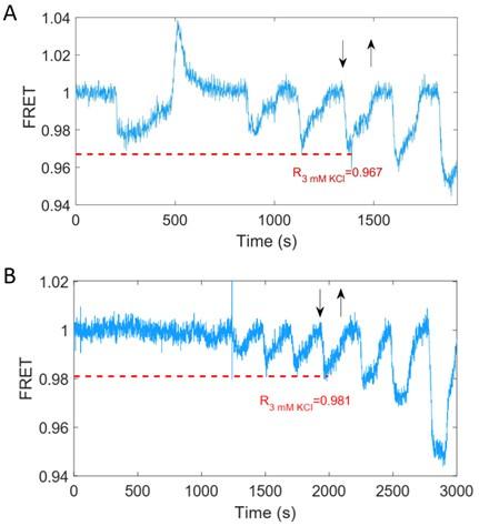
The authors show the FRET data with both KCl and K2SO4, concluding that the chemotactic response mainly resulted from potassium ions. However, this was only measured by FRET. It would be more convincing if the motility assay in Fig1 is also performed with K2SO4. The authors did not address this point. In light of complications associated with the use of the FRET sensor, this experiment is more important.
We thank the reviewer for the suggestion. We agree that additional confirmation with a motility assay is important. To address this, we have now measured the response of the motor rotational signal to 15 mM K2SO4 using the bead assay and compared it with the response to 30 mM KCl. The results are shown in Fig. S2. The response of motor CW bias to 15 mM K2SO4 exhibited an attractant response, characterized by a decreased CW bias upon the addition of K2SO4, followed by an over-adaptation that is qualitatively similar to the response to 30 mM KCl. However, there were notable differences in the adaptation time and the presence of an overshoot. Specifically, the adaptation time to K2SO4 was shorter compared to that for KCl, and there was a notable overshoot in the CW bias during the adaptation phase. These differences may have resulted from the weaker response to K2SO4 (Fig. S1B) and additional modifications due to CysZ-mediated cellular uptake of sulfate (Zhang et al., Biochimica et Biophysica Acta 1838,1809–1816 (2014)). The faster adaptation and overshoot complicated the chemotactic drift in the microfluidic assay as in Fig. 1, such that we were unable to observe a noticeable drift in a K2SO4 gradient under the same experimental conditions used for the KCl gradient.
The response of motor rotational signal to 15 mM K2SO4 has been added to Fig. S2.
Recommendations for the authors:
Reviewer #1 (Recommendations For The Authors):
(1) The response curve and adaptation level/time in the main text (Fig. 4) should be replaced by the corrected counterparts (currently in Fig. S5). The current version is especially confusing because Fig. 6 shows the corrected response, but the difference from Fig. 4 is not mentioned.
We thank the reviewer for the suggestion. We have now merged the results of the original Fig. S5 into Fig. 4.
a. The discussion of the uncorrected response with small hill coefficient and potentially negative cooperativity was left in the text (lines 223-234), but the new measurements show this is not true for the actual response. This should be removed or significantly rephrased.
We thank the reviewer for the suggestion. We have now removed the statement about potentially negative cooperativity and added the corrected results for the actual response.
(2) It may be helpful to restate the definition of f_m in the methods (near Eq. 3-4).
Thank you for the suggestion. We have now restated the definition of fm and fL below Eq. 3-4: “In the denominator on the right-hand side of Eq. 3, the two terms within the parentheses of exponential expression represent the methylation-dependent (fm) and ligand-dependent (fL) free energy, respectively.”
Author response:
The following is the authors’ response to the previous reviews.
Reviewer #2:
(1) The use of two m<sup>5</sup>C reader proteins is likely a reason for the high number of edits introduced by the DRAM-Seq method. Both ALYREF and YBX1 are ubiquitous proteins with multiple roles in RNA metabolism including splicing and mRNA export. It is reasonable to assume that both ALYREF and YBX1 bind to many mRNAs that do not contain m<sup>5</sup>C.
To substantiate the author's claim that ALYREF or YBX1 binds m<sup>5</sup>C-modified RNAs to an extent that would allow distinguishing its binding to non-modified RNAs from binding to m<sup>5</sup>C-modified RNAs, it would be recommended to provide data on the affinity of these, supposedly proven, m<sup>5</sup>C readers to non-modified versus m<sup>5</sup>C-modified RNAs. To do so, this reviewer suggests performing experiments as described in Slama et al., 2020 (doi: 10.1016/j.ymeth.2018.10.020). However, using dot blots like in so many published studies to show modification of a specific antibody or protein binding, is insufficient as an argument because no antibody, nor protein, encounters nanograms to micrograms of a specific RNA identity in a cell. This issue remains a major caveat in all studies using so-called RNA modification reader proteins as bait for detecting RNA modifications in epitranscriptomics research. It becomes a pertinent problem if used as a platform for base editing similar to the work presented in this manuscript.
The authors have tried to address the point made by this reviewer. However, rather than performing an experiment with recombinant ALYREF-fusions and m<sup>5</sup>C-modified to unmodified RNA oligos for testing the enrichment factor of ALYREF in vitro, the authors resorted to citing two manuscripts. One manuscript is cited by everybody when it comes to ALYREF as m<sup>5</sup>C reader, however none of the experiments have been repeated by another laboratory. The other manuscript is reporting on YBX1 binding to m<sup>5</sup>C-containing RNA and mentions PAR-CLiP experiments with ALYREF, the details of which are nowhere to be found in doi: 10.1038/s41556-019-0361-y.<br /> Furthermore, the authors have added RNA pull-down assays that should substitute for the requested experiments. Interestingly, Figure S1E shows that ALYREF binds equally well to unmodified and m<sup>5</sup>C-modified RNA oligos, which contradicts doi:10.1038/cr.2017.55, and supports the conclusion that wild-type ALYREF is not specific m<sup>5</sup>C binder. The necessity of including always an overexpression of ALYREF-mut in parallel DRAM experiments, makes the developed method better controlled but not easy to handle (expression differences of the plasmid-driven proteins etc.)
Thank you for pointing this out. First, we would like to correct our previous response: the binding ability of ALYREF to m<sup>5</sup>C-modified RNA was initially reported in doi: 10.1038/cr.2017.55, (and not in doi: 10.1038/s41556-019-0361-y), where it was observed through PAR-CLIP analysis that the K171 mutation weakens its binding affinity to m<sup>5</sup>C -modified RNA.
Our previous experimental approach was not optimal: the protein concentration in the INPUT group was too high, leading to overexposure in the experimental group. Additionally, we did not conduct a quantitative analysis of the results at that time. In response to your suggestion, we performed RNA pull-down experiments with YBX1 and ALYREF, rather than with the pan-DRAM protein, to better validate and reproduce the previously reported findings. Our quantitative analysis revealed that both ALYREF and YBX1 exhibit a stronger affinity for m<sup>5</sup>C -modified RNAs. Furthermore, mutating the key amino acids involved in m<sup>5</sup>C recognition significantly reduced the binding affinity of both readers. These results align with previous studies (doi: 10.1038/cr.2017.55 and doi: 10.1038/s41556-019-0361-y), confirming that ALYREF and YBX1 are specific readers of m<sup>5</sup>C -modified RNAs. However, our detection system has certain limitations. Despite mutating the critical amino acids, both readers retained a weak binding affinity for m<sup>5</sup>C, suggesting that while the mutation helps reduce false positives, it is still challenging to precisely map the distribution of m<sup>5</sup>C modifications. To address this, we plan to further investigate the protein structure and function to obtain a more accurate m<sup>5</sup>C sequencing of the transcriptome in future studies. Accordingly, we have updated our results and conclusions in lines 294-299 and discuss these limitations in lines 109-114.
In addition, while the m<sup>5</sup>C assay can be performed using only the DRAM system alone, comparing it with the DRAM<sup>mut</sup>C control enhances the accuracy of m<sup>5</sup>C region detection. To minimize the variations in transfection efficiency across experimental groups, it is recommended to use the same batch of transfections. This approach not only ensures more consistent results but also improve the standardization of the DRAM assay, as discussed in the section added on line 308-312.
(2) Using sodium arsenite treatment of cells as a means to change the m<sup>5</sup>C status of transcripts through the downregulation of the two major m<sup>5</sup>C writer proteins NSUN2 and NSUN6 is problematic and the conclusions from these experiments are not warranted. Sodium arsenite is a chemical that poisons every protein containing thiol groups. Not only do NSUN proteins contain cysteines but also the base editor fusion proteins. Arsenite will inactivate these proteins, hence the editing frequency will drop, as observed in the experiments shown in Figure 5, which the authors explain with fewer m<sup>5</sup>C sites to be detected by the fusion proteins.
The authors have not addressed the point made by this reviewer. Instead the authors state that they have not addressed that possibility. They claim that they have revised the results section, but this reviewer can only see the point raised in the conclusions. An experiment would have been to purify base editors via the HA tag and then perform some kind of binding/editing assay in vitro before and after arsenite treatment of cells.
We appreciate the reviewer’s insightful comment. We fully agree with the concern raised. In the original manuscript, our intention was to use sodium arsenite treatment to downregulate NSUN mediated m<sup>5</sup>C levels and subsequently decrease DRAM editing efficiency, with the aim of monitoring m<sup>5</sup>C dynamics through the DRAM system. However, as the reviewer pointed out, sodium arsenite may inactivate both NSUN proteins and the base editor fusion proteins, and any such inactivation would likely result in a reduced DRAM editing. This confounds the interpretation of our experimental data.
As demonstrated in Appendix A, western blot analysis confirmed that sodium arsenite indeed decreased the expression of fusion proteins. In addition, we attempted in vitro fusion protein purification using multiple fusion tags (HIS, GST, HA, MBP) for DRAM fusion protein expression, but unfortunately, we were unable to obtain purified proteins. However, using the Promega TNT T7 Rapid Coupled In Vitro Transcription/Translation Kit, we successfully purified the DRAM protein (Appendix B). Despite this success, subsequent in vitro deamination experiments did not yield the expected mutation results (Appendix C), indicating that further optimization is required. This issue is further discussed in line 314-315.
Taken together, the above evidence supports that the experiment of sodium arsenite treatment was confusing and we determined to remove the corresponding results from the main text of the revised manuscript.
Author response image 1.
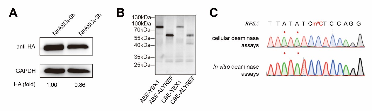
(3) The authors should move high-confidence editing site data contained in Supplementary Tables 2 and 3 into one of the main Figures to substantiate what is discussed in Figure 4A. However, the data needs to be visualized in another way then excel format. Furthermore, Supplementary Table 2 does not contain a description of the columns, while Supplementary Table 3 contains a single row with letters and numbers.
The authors have not addressed the point made by this reviewer. Figure 3F shows the screening process for DRAM-seq assays and principles for screening high-confidence genes rather than the data contained in Supplementary Tables 2 and 3 of the former version of this manuscript.
Thank you for your valuable suggestion. We have visualized the data from Supplementary Tables 2 and 3 in Figure 4A as a circlize diagram (described in lines 213-216), illustrating the distribution of mutation sites detected by the DRAM system across each chromosome. Additionally, to improve the presentation and clarity of the data, we have revised Supplementary Tables 2 and 3 by adding column descriptions, merging the DRAM-ABE and DRAM-CBE sites, and including overlapping m<sup>5</sup>C genes from previous datasets.
Author response:
The following is the authors’ response to the previous reviews
Reviewer #1 (Public review):
Summary:
Liver cancer shows a high incidence in males than females with incompletely understood causes. This study utilized a mouse model that lacks the bile acid feedback mechanisms (FXR/SHP DKO mice) to study how dysregulation of bile acid homeostasis and a high circulating bile acid may underlie the gender-dependent prevalence and prognosis of HCC. By transcriptomics analysis comparing male and female mice, unique sets of gene signatures were identified and correlated with HCC outcomes in human patients. The study showed that ovariectomy procedure increased HCC incidence in female FXR/SHP DKO mice that were otherwise resistant to agedependent HCC development, and that removing bile acids by blocking intestine bile acid absorption reduced HCC progression in FXR/SHP DKO mice. Based on these findings, the authors suggest that gender-dependent bile acid metabolism may play a role in the male-dominant HCC incidence, and that reducing bile acid level and signaling may be beneficial in HCC treatment.
strengths:
(1) Chronic liver diseases often proceed the development of liver and bile duct cancer. Advanced chronic liver diseases are often associated with dysregulation of bile acid homeostasis and cholestasis. This study takes advantage of a unique FXR/SHP DKO model that develop high organ bile acid exposure and spontaneous age-dependent HCC development in males but not females to identify unique HCC-associated gene signatures. The study showed that the unique gene signature in female DKO mice that had lower HCC incidence also correlated with lower grade HCC and better survival in human HCC patients. 2. The study also suggests that differentially regulated bile acid signaling or gender-dependent response to altered bile acids may contribute to gender-dependent susceptibility to HCC development and/or progression. 3. The sex-dependent differences in bile acidmediated pathology clearly exist but are still not fully understood at the mechanistic level. Female mice have been shown to be more sensitive to bile acid toxicity in a few cholestasis models, while this study showed a male dominance of bile acid promotion of HCC. This study used ovariectomy to demonstrate that female hormones are possible underlying factors. Future studies are needed to understand the interaction of sex hormones, bile acids, and chronic liver diseases and cancer.
We thank Reviewer 1 for their positive and thorough assessment of our manuscript
Weaknesses:
(1) HCC shows heterogeneity, and it is unclear what tissues (tumor or normal) were used from the DKO mice and human HCC gene expression dataset to obtain the gene signature, and how the authors reconcile these gene signatures with HCC prognosis.
Mice studies: Aged DKO mice develop aggressive tumors (major and minor nodules, See Figure 1), and the entire liver is burdened with multiple tumor nodules. It is technically challenging to demarcate the tumor boundaries as most of the surrounding tissues do not display normal tissue architecture. Therefore, livers from age- and sexmatched wild-type C57/BL6 mice were used as control tissue. All the mice were inbred in our facility. Spatial transcriptomics and longitudinal studies are ongoing to collect tumors at earlier time points wherein we can differentiate tumor and non-tumor tissue.
Human Studies: We mined five separate clinical data sets. The human HCC gene expression comprised of samples from the (i) National Cancer Institute (NCI) cohort (GEO accession numbers, GSE1898 and GSE4024) and (ii) Korea, (iii) Samsung, (iv) Modena, and (v) Fudan cohorts as previously described (GEO accession numbers, GSE14520, GSE16757, GSE43619, GSE36376, and GSE54236). We have added a new supplemental table 4, giving details of these datasets. Depending on the cohort, they are primarily HCC samples- surgical resections of HCC, control samples, with some tumors and paired non-tumor tissues.
(2) The authors identified a unique set of gene expression signatures that are linked to HCC patient outcomes, but analysis of these gene sets to understand the causes of cancer promotion is still lacking. The studies of urea cycle metabolism and estrogen signaling were preliminary and inconclusive. These mechanistic aspects may be followed up in revision or future studies.
We agree. Experiments to elicit HCC causality and promotion are complex, given the heterogeneous nature of liver cancer. Moreover, the length of time (12 months) needed to spontaneously develop cancer in this DKO mouse model makes it challenging. As mentioned by the reviewer, mechanistic studies are ongoing, and longitudinal time course experiments are actively being pursued to delineate causality. Having said that, we mined the TCGA LIHC (The Cancer Genome Atlas Liver Hepatocellular Carcinoma) database to examine the expression of the individual urea cycle genes and found them suppressed in liver tumorigenesis (new Supplementary Figure 4). We also evaluated if estrogen receptor (Er) targets altered in DKO females (DKO_Estrogen) correlate with overall survival in HCC (new Supplementary Figure 6). We note that Er expression per se is reduced in males and females upon liver tumorigenesis. Also, DKO_Estrogen signature positively corroborated with better overall survival (new Supplementary Figure 6). These findings further bolster the relevance of urea cycle metabolism and estrogen signaling during HCC.
(3) While high levels of bile acids are convincingly shown to promote HCC progression, their role in HCC initiation is not established. The DKO model may be limited to conditions of extremely high levels of organ bile acid exposure. The DKO mice do not model the human population of HCC patients with various etiology and shared liver pathology (i.e. cirrhosis). Therefore, high circulating bile acids may not fully explain the male prevalence of HCC incidence.
We agree with this comment that our studies do not show bile acids can initiate HCC and may act as one of the many factors that contribute to the high male prevalence of HCC. This is exactly the reason why throughout the manuscript we do not write about HCC initiation. To clarify further, in the revised discussion of the manuscript, we have added a sentence to highlight this aspect, “while this study demonstrates bile acids promote HCC progression it does not investigate or provide evidence if excess bile acids are sufficient for HCC initiation.”
(4) The authors showed lower circulating bile acids and increased fecal bile acid excretion in female mice and hypothesized that this may be a mechanism underlying the lower bile acid exposure that contributed to lower HCC incidence in female DKO mice. Additional analysis of organ bile acids within the enterohepatic circulation may be performed because a more accurate interpretation of the circulating bile acids and fecal bile acids can be made in reference to organ bile acids and total bile acid pool changes in these mice.
As shown in this manuscript- we provide BA compositional analyses from the liver, serum, urine, and feces (Figures 5 and 6, new Supplementary Figure 8, Supplementary Tables 4 and 5). Unfortunately, we did not collect the intestinal tissue or gallbladders for BA analysis in this study. Separate cohorts of mice are being aged for future BA analyses from different organs within the enterohepatic loop. We thank you for this suggestion. Nevertheless, we have previously measured and reported BA values to be elevated in the intestines and the gall bladder of young DKO mice (PMC3007143).
Reviewer #2 (Public review):
Weaknesses:
(1) The translational value to human HCC is not so strong yet. Authors show that there is a correlation between the female-selective gene signature and low-grade tumors and better survival in HCC patients overall. However, these data do not show whether this signature is more highly correlated with female tumor burden and survival. In other words, whether the mechanisms of female protection may be similar between humans and mice. In that respect, it would also be good to elaborate on whether women have higher fecal BA excretion and lower serum BA concentration.
The reviewer poses an interesting question to test if the DKO female-specific signatures are altered differently in male vs. female HCC samples. As we found the urea cycle and estrogen signaling to be protective and enriched in our mouse model, we tested their expression pattern using the TCGA-LIHC RNA-seq data. We found urea cycle genes and Er transcripts broadly reduced in tumor samples irrespective of the sex (new Supplementary Figure 4 and Supplementary Figure 6), indicating that these pathways are compromised upon tumorigenesis even in the female livers.
While prior studies have shown (i) a smaller BA pool w synthesis in men than women (PMID: 22003820), we did not find a study that systematically investigated BA excretion between the sexes in HCC context. The reviewer is spot on in suggesting BA analysis from HCC and unaffected human fecal samples from both sexes. Designing and performing such studies in the future will provide concrete proof of whether BA excretion protects female livers from developing liver cancer. We thank you for these suggestions.
(2) The authors should perform a thorough spelling and grammar check.
We apologize for the typos, which have been fixed, and as suggested by the reviewer, we have performed a grammar check.
(3) There are quite some errors and inaccuracies in the result section, figures, and legends. The authors should correct this.
We apologize for the inadvertent errors in the manuscript, and we have clarified these inaccuracies in the revised version. Thank you.
Reviewer#1 (Recommendations for the authors).
(1) Figures 1A-F, This statement of altered liver steatosis needs to be further supported by measurement of liver triglycerides. Lower magnification images of Sirius red stain should be shown for better evaluation of liver fibrosis.
Unfortunately, we did not measure liver triglycerides and sirius red stained samples have faded, and lower magnification is unavailable at this juncture. We have modified our results accordingly.
We did not take the gross picture of WT female and DKO female livers in the same frame as shown below. Since the manuscript is focused on male and female differences in liver cancer incidence, we provided DKO male and female liver images as Figure 1D in the paper.
Author response image 1.
Gross liver images of a year-old WT and DKO mice which show prominent hepatocarcinogenesis in DKO male mice
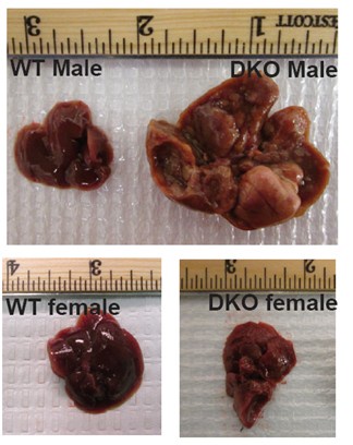
(2) Can the authors clarify if the gene transcriptomics was performed with normal or tumor tissues of DKO mice?
Gene transcriptomics were performed with the tumor tissue of DKO mice. We have previously published data from younger non tumor bearing DKO male mice (PMCID: PMC3007143).
(3) Supplementary Figure 3C. Could the authors confirm if this is F vs M or just DKO female since it does not seem to match the result description in the main text? It is better practice to indicate the sub-panels of the Supplementary Figures in the main text while describing the results.
As the reviewer correctly points out Supplementary Figure 3C is DKO F vs M signature not DKO_female signature and this has been clarified in the text. We have also included DKO_F data now to reduce the confusion.
(4) Figure 3. Legend, the data presented are not well explained in the Legend, especially the labeling and what is being presented and compared.
As suggested by the reviewer, we have modified the legend accordingly.
(5) Supplementary Table 4 does not contain total serum bile acid as described in the main text.
We agree with the reviewer. We provided primary and secondary BA concentrations, Supplementary Table 4 (currently Supplementary Table 5 in the revised version): Rows 20 and 21. but not their added total. We have modified the text accordingly.
(6) Method section: many experiments lack descriptions of details.
We have added details to the animal experimental design, ER ChIP-PCR, schematics of experiments are included within the main and supplemental figures, metabolomics and BA analysis have been expanded.
Reviewer #2 (Recommendations For The Authors):
General:
(1) The authors are advised to do a thorough grammar and spelling check.
We have performed spelling and grammar check as suggested using an online platform Grammarly. Thank You.
Results:
(1) Figure 1 o The authors should show in Figure 1D female WT and female DKO liver.
See Figure 1 added in our responses to point 1 of reviewer 1’s comment.
In the Figure legend, (A-E) should be replaced by (A+D).
Thank you. We have modified it accordingly.
The authors do not refer to 1J in the text, please add this reference.
Thank you for pointing it. We have referenced 1J in the text.
The description of 1H does not elaborate on the sex differences in ALT/AST levels, as this is the focus of the manuscript.
We have added a sentence to show that the injury markers are higher in DKO males, which is consistent with an advanced disease. Thanks.
The authors should use the correct nomenclature in Figure 1I/1J (gene vs protein and capitals vs non-capitals).
The Figure 1I and 1J show gene expression of Fxr and Shp and hence we used the non-capital italicized nomenclature. Thanks.
(2) Figure 2:
The x-axis length is different in Figures 2A and 2B. Please correct to visualize the differences between males and females better.
The x axis length has been fixed as suggested. Thanks
(3) Figure 3:
The authors should elaborate on how the patients were assigned to each gene signature. This is not fully clear.
The gene set obtained from the WT and DKO mice were used. The process used is shown as a schematic in Supplemental Fig 2C and the gene list is included in an excel sheet as Supplemental table 1.
We are curious how these data (F3A-C) would look when separating male and female human patients.
We performed an overall survival analysis with a subgroup of patients and provide it. We segregated the HCC cohort data on sex and age (>55 yr, since we assumed 55 as an age for menopause) and evaluated the DKO gene signature. Similar to the original figure 3, we find that irrespective of sex, and age, DKO FvsM gene signature corresponds with better overall survival in men and in women. These findings align with the combined analysis in overall survival shown in original Figure 3 of the manuscript, and therefore we did not modify it. If deemed necessary, we are happy to include the figure below to reviewers in the main manuscript.
Author response image 2.
Correlation of gene signatures obtained from WT and DKO mouse model with the survival data of HCC patients segregated by age and sex. The Kaplan Meier Survival graphs were generated based on WT and DKO transcriptome changes using five HCC clinical cohorts. Analysis of OS (Overall Survival) in patients ((A) Men and (B) Women) using the gene signatures representative of either male WT or male DKO, female WT or female DKO, and unique changes observed in female DKO mice but not in male DKO mice.
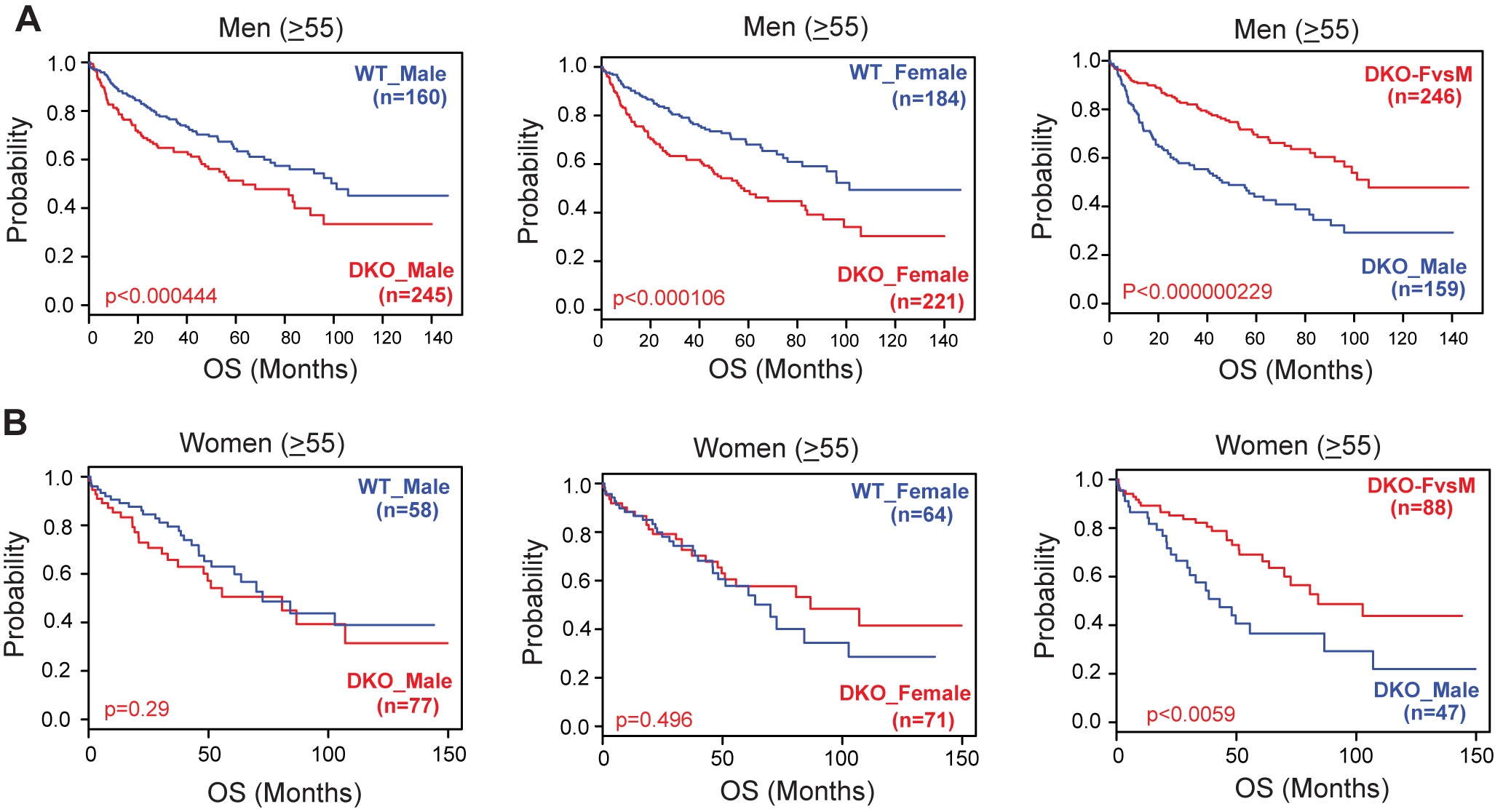
What was used as the control signature in Figure 3C? Please specify this.
For Figure 3C we compared the DKO_M signature to that of DKOF vs M signature. These genes are listed as an Excel Sheet (Supplementary Table 1).
The authors claim that DKO female mice display chronic cholestasis, similar to their male counterparts. Please refer to previous work or show the data.
Serum BA levels are elevated in DKO females are reported in supplementary table 5 and we find comparable hepatic BA composition in Figure 5 F.
(4) Figure 4: Labels for the x-axis are missing in Figure 4C. Please add legends or labels to the bars.
The x axis label is included in the top Serum BAs in (M)
In Figure 4I, the percentage of input is quite low. An IgG control would show whether recruitment of ERalpha to the shown loci is significant above background levels. Also, ChIP on the OVX liver could serve as a negative control.
We did use IgG as control pull down and the signals above this background were considered. We have not performed this in OVX, which would be an excellent negative control for future studies. Thank You.
The results and legends refer to ChIP-qPCR, while methods only mention ChIP-seq.Please adapt.
We sincerely apologize for the mistake. We used published ChIP-seq to identify putative binding site and then performed ChIP PCR to validate it. We have clarified and rectified this error. Thank You.
Significance indications in the figure legend do not correspond with significance indications in the figure. Please explain the used significance symbols in the figure in the legend.
Thank You. The legends and their significance have been matched.
(5) Figure 5:
Authors claim lowered total serum BA in females compared to males, and reference to Supplementary Table 4. However, these data are not provided, only percentages and ratios are displayed.
In the revised version, this has become Table 5. See response to the same concern noted by Reviewer 1, Point 5 above.
Figure 5D: Are sulphated BA also elevated in WT females? Please provide these data.
There is no significant urinary excretion of BAs in WT control animals. We have previously measured and found none. But under cholestatic conditions BAs are observed in urine. Therefore, sulphated BA levels were found only in the DKO mice.
Figure 5H: Is the fecal BA excretion in WT females also proportionally higher than in males? Please provide these data.
We were unable to perform the untargeted metabolomics profiling of WT fecal samples. When we measured for BAs in the feces, as expected very low conc were present irrespective of the sex (~0.01 M) and we did not find any sex difference. Also, prior studies in 129SVJ strain exhibited comparable fecal excretion (PMC150802). We did not find any clinical studies that measured fecal BA between the sexes.
(6) Figure 6:
References in the text of the result section to Figure 6 are wrong. The authors should change this.
Thank You. This has been rectified.
Significance indications in the legend do not correspond with significance indications in the figure. Please explain the used significance symbols in the figure in the legend.
Thank You. The legends and their significance have been matched.
(7) Supplemental Figure 3:
Please adapt the title of this figure; the sentence is incorrect. The description of this figure is very poor.
We have modified the legend and the title of the Supplemental Figure 3 to make it more appropriate. Thanks
Please explain what the blue and red dots represent.
Each dot in blue and yellow indicate the Bayesian probability generated from our BCCP model.
What are the bold horizontal lines representing? Why are there no dots in some box plots? Please elaborate.
The box represents the interquartile range (IQR), encompassing the middle 50% of the data. The bottom and top edges correspond to the 25th and 75th percentiles, respectively, while the bold horizontal line indicates the median value.
The absence of visible dots in certain categories—particularly in higher CLIP and TNM stages—is due to the small number of patients, all of whom had similar Bayesian prediction probabilities. As these values cluster tightly around the median, the individual dots may be overlapped and hidden behind the median line.
The figure is not visually easy to understand, please reconsider the representation.
We hope the modified figure legends with the explanation of the lines and the points in the graphs increases the clarity and makes them acceptable.
Please add the DKO_female signature plot.
We have added these graph to Supplemental figure 3
(8) Supplemental 4A:
Fold change at Z-score is missing. This should be added.
Thank you we have added this information
(9) Supplemental 5:
The scale bar is missing. This should be included.
The figure is now supplemental figure 8 and the scale bar has been added.
Methods:
(1) Did the authors use ChIP-sequencing or ChIP-qPCR? Please describe the correct method.
We apologize for the error. We have used ChIP-PCR and rectified it in our methods and in our response to a figure 4 query.
(2) It is unclear how the mouse model was generated. Please refer to earlier publications.
The mice were generated in house at UIUC, and we have added this sentence to the Methods section. The original reference has been cited in the text (PMCID: PMC3007143).
Discussion:
(1) The authors claim in the discussion: 'consistently higher recruitment of ER to the classical BA synthetic genes ...' This is not shown in Figure 4I, only ER recruitment to Cyp7a1 is significantly higher in females. Please rephrase.
We agree and we have modified the sentence Cyp7A1 accounts for ~75% of BA synthesis and is a rate-limiting gene in the classical BA synthesis pathway.
(2) The authors could make their statements stronger if they could elaborate on whether women have more fecal BA excretion, and if there are differences in serum BA concentration in HCC between male and female patients.
Unfortunately, we were unable to find clinical studies with appropriate controls which examined and reported serum BA in HCC in a sex specific manner.
In addition, to understand whether the female-specific protections in humans are similar to mice, it would be nice to show correlations of the female-specific mouse signature with male and female liver signatures.
At this time, we do not have large n numbers of control or precancerous early-stage patient datasets from both sexes to make such comparisons. Nevertheless, there is translational relevance of these sex-specific signature. Figure 2 included in the reviewer response shows that DKO male signature correlates with poor overall survival in males, whereas neither DKO male nor DKO female signature predict outcome in females. In contrast, DKO female-specific gene signature (DKOFvsM) correlates with better overall survival in both men and in women.
(3) The authors state in the discussion: 'Currently we do not know how to reconcile this data other than indicating a potential ER independent mechanism.' We do not understand the reasoning behind this statement. Please clarify.
We find that increased Erα expression in DKO coincides with CA-mediated suppression of BA synthesis genes in the absence of Fxr and Shp. But we also noticed that in OVX DKO mice, Erα expression is blunted, and so is basal BA synthesis gene expression. Putting together these data, it is intriguing that Erα expression correlates both positively and negatively with BA synthesis genes. To reconcile these contrasting results, we have written the following sentence in the discussion.
“These findings suggest Erα expression is linked to both positive and negative regulation of BA synthesis genes. But we do not know how ER elicits these differential effects on BA synthesis.”
Author response:
The following is the authors’ response to the previous reviews.
Public Reviews:
Reviewer #2 (Public Review):
Summary:
The manuscript by Kelbert et al. presents results on the involvement of the yeast transcription factor Sfp1 in the stabilisation of transcripts whose synthesis it stimulates. Sfp1 is known to affect the synthesis of a number of important cellular transcripts, such as many of those that code for ribosomal proteins. The hypothesis that a transcription factor can remain bound to the nascent transcript and affect its cytoplasmic half-life is attractive. However, the association of Sfp1 with cytoplasmic transcripts remains to be validated, as explained in the following comments:
A two-hybrid based assay for protein-protein interactions identified Sfp1, a transcription factor known for its effects on ribosomal protein gene expression, as interacting with Rpb4, a subunit of RNA polymerase II. Classical two-hybrid experiments depend on the presence of the tested proteins in the nucleus of yeast cells, suggesting that the observed interaction occurs in the nucleus. Unfortunately, the two-hybrid method cannot determine whether the interaction is direct or mediated by nucleic acids. The revised version of the manuscript now states that the observed interaction could be indirect.
To understand to which RNA Sfp1 might bind, the authors used an N-terminally tagged fusion protein in a cross-linking and purification experiment. This method identified 264 transcripts for which the CRAC signal was considered positive and which mostly correspond to abundant mRNAs, including 74 ribosomal protein mRNAs or metabolic enzyme-abundant mRNAs such as PGK1. The authors did not provide evidence for the specificity of the observed CRAC signal, in particular what would be the background of a similar experiment performed without UV cross-linking. This is crucial, as Figure S2G shows very localized and sharp peaks for the CRAC signal, often associated with over-amplification of weak signal during sequencing library preparation.
(1) To rule out possible PCR artifacts, we used a UMI (Unique Molecular Identifier) scan. UMIs are short, random sequences added to each molecule by the 5’ adapter to uniquely tag them. After PCR amplification and alignment to the reference genome, groups of reads with identical UMIs represent only one unique original molecule. Thus, UMIs allow distinguishing between original molecules and PCR duplicates, effectively eliminating the duplicates.
(2) Looking closely at the peaks using the IGV browser, we noticed that the reads are by no means identical. Each carrying a mutation [probably due to the cross-linking] in a different position and having different length. Note that the reads are highly reproducible in two replicate.
(3) CRAC+ genes do not all fall into the category of highly transcribed genes. On the contrary, as depicted in Figure 6A (green dots), it is evident that CRAC+ genes exhibit a diverse range of Rpb3 ChIP and GRO signals. Furthermore, as illustrated in Figure 7A, when comparing CRAC+ to Q1 (the most highly transcribed genes), it becomes evident that the Rpb4/Rpb3 profile of CRAC+ genes is not a result of high transcription levels.
(4) Only a portion of the RiBi mRNAs binds Sfp1, despite similar expression of all RiBi.
(5) The CRAC+ genes represent a distinct group with many unique features. Moreover, many CRAC+ genes do not fall into the category of highly transcribed genes.
(6) The biological significance of the 262 CRAC+ mRNAs was demonstrated by various experiments; all are inconsistent with technical flaws. Some examples are:
a) Fig. 2a and B show that most reads of CRAC+ mRNA were mapped to specific location – close the pA sites.
b) Fig. 2C shows that most reads of CRAC+ mRNA were mapped to specific RNA motif.
c) Most RiBi CRAC+ promoter contain Rap1 binding sites (p= 1.9x10⁻²²), whereas the vast majority of RiBi CRAC- promoters do not contain Rap1 binding site. (Fig. 3C).
d) Fig. 4A shows that RiBi CRAC+ mRNAs become destabilized due to Sfp1 deletion, whereas RiBi CRAC- mRNAs do not. Fig. 4B shows similar results due to
e) Fig. 6B shows that the impact of Sfp1 on backtracking is substantially higher for CRAC+ than for CRAC- genes. This is most clearly visible in RiBi genes.
f) Fig. 7A shows that the Sfp1-dependent changes along the transcription units is substantially more rigorous for CRAC+ than for CRAC-.
g) Fig. S4B Shows that chromatin binding profile of Sfp1 is different for CRAC+ and CRAC- genes
In a validation experiment, the presence of several mRNAs in a purified SFP1 fraction was measured at levels that reflect the relative levels of RNA in a total RNA extract. Negative controls showing that abundant mRNAs not found in the CRAC experiment were clearly depleted from the purified fraction with Sfp1 would be crucial to assess the specificity of the observed protein-RNA interactions (to complement Fig. 2D).
GPP1, a highly expressed genes, is not to be pulled down by Sfp1 (Fig. 2D). GPP1 (alias RHR2) was included in our Table S2 as one of the 264 CRAC+ genes, having a low CRAC value. However, when we inspected GPP1 results using the IGV browser, we realized that the few reads mapped to GPP1 are actually anti-sense to GPP1 (perhaps they belong to the neighboring RPL34B genes, which is convergently transcribed to GPP1) (see Fig. 1 at the bottom of the document). Thus, GPP1 is not a CRAC+ gene and would now serve as a control. See We changed the text accordingly (see page 11 blue sentences). In light of this observation, we checked other CRAC genes and found that, except for ALG2, they all contain sense reads (some contain both sense and anti-sense reads). ALG2 and GPP1 were removed leaving 262 CRAC+ genes.
The CRAC-selected mRNAs were enriched for genes whose expression was previously shown to be upregulated upon Sfp1 overexpression (Albert et al., 2019). The presence of unspliced RPL30 pre-mRNA in the Sfp1 purification was interpreted as a sign of co-transcriptional assembly of Sfp1 into mRNA, but in the absence of valid negative controls, this hypothesis would require further experimental validation. Also, whether the fraction of mRNA bound by Sfp1 is nuclear or cytoplasmic is unclear.
Further experimental validation was provided in some of our figures (e.g., Fig. 5C, Fig. 3B).
We argue that Sfp1 binds RNA co-transcriptionally and accompanies the mRNA till its demise in the cytoplasm: Co-transcriptional binding is shown in: (I) a drop in the Sfp1 ChIP-exo signal that coincides with the position of Sfp1 binding site in the RNA (Fig. 5C), demonstrating a movement of Sfp1 from chromatin to the transcript, (II) the dependence of Sfp1 RNA-binding on the promoter (Fig. 3B) and binding of intron-containing RNA. Taken together these 3 different experiments demonstrate that Sfp1 binds Pol II transcript co-transcriptionally. Association of Sfp1 with cytoplasmic mRNAs is shown in the following experiments: (I) Figure 2D shows that Sfp1 pulled down full length RNA, strongly suggesting that these RNA are mature cytoplasmic mRNAs. (II) mRNA encoding ribosomal proteins, which belong to the CRAC+ mRNAs group are degraded by Xrn1 in the cytoplasm (Bresson et al., Mol Cell 2020). The capacity of Sfp1 to regulates this process (Fig. 4A-D) is therefore consistent with cytoplasmic activity of Sfp1. (III) The effect of Sfp1 on deadenylation (Fig. 4D), a cytoplasmic process, is also consistent with cytoplasmic activity of Sfp1.
To address the important question of whether co-transcriptional assembly of Spf1 with transcripts could alter their stability, the authors first used a reporter system in which the RPL30 transcription unit is transferred to vectors under different transcriptional contexts, as previously described by the Choder laboratory (Bregman et al. 2011). While RPL30 expressed under an ACT1 promoter was barely detectable, the highest levels of RNA were observed in the context of the native upstream RPL30 sequence when Rap1 binding sites were also present. Sfp1 showed better association with reporter mRNAs containing Rap1 binding sites in the promoter region. Removal of the Rap1 binding sites from the reporter vector also led to a drastic decrease in reporter mRNA levels. Co-purification of reporter RNA with Sfp1 was only observed when Rap1 binding sites were included in the reporter. Negative controls for all the purification experiments might be useful.
In the swapping experiment, the plasmid lacking RapBS serves as the control for the one with RapBS and vice versa (see Bregman et al., 2011). Remember, that all these contracts give rise to identical RNA. Indeed, RabBS affects both mRNA synthesis and decay, therefore the controls are not ideal. However, see next section.
More importantly, in Fig. 3B “Input” panel, one can see that the RNA level of “construct F” was higher than the level of “construct E”. Despite this difference, only the RNA encoded by construct E was detected in the IP panel. This clearly shows that the detection of the RNA was not merely a result of its expression level.
To complement the biochemical data presented in the first part of the manuscript, the authors turned to the deletion or rapid depletion of SFP1 and used labelling experiments to assess changes in the rate of synthesis, abundance and decay of mRNAs under these conditions. An important observation was that in the absence of Sfp1, mRNAs encoding ribosomal protein genes not only had a reduced synthesis rate, but also an increased degradation rate. This important observation needs careful validation,
Indeed, we do provide validations in Fig. 4C Fig. 4D Fig. S3A and during the revision we included an additional validation as Fig. S3B. Of note, we strongly suspect that GRO is among the most reliable approaches to determine half-lives (see our response in the first revision letter).
As genomic run-on experiments were used to measure half-lives, and this particular method was found to give results that correlated poorly with other measures of half-life in yeast (e.g. Chappelboim et al., 2022 for a comparison). As an additional validation, a temperature shift to 42{degree sign}C was used to show that , for specific ribosomal protein mRNA, the degradation was faster, assuming that transcription stops at that temperature. It would be important to cite and discuss the work from the Tollervey laboratory showing that a temperature shift to 42{degree sign}C leads to a strong and specific decrease in ribosomal protein mRNA levels, probably through an accelerated RNA degradation (Bresson et al., Mol Cell 2020, e.g. Fig 5E).
This was cited. Thank you.
Finally, the conclusion that mRNA deadenylation rate is altered in the absence of Sfp1, is difficult to assess from the presented results (Fig. 3D).
This type of experiment was popular in the past. The results in the literature are similar to ours (in fact, ours are nicer). Please check the papers cited in our MS and a number of papers by Roy Parker.
The effects of SFP1 on transcription were investigated by chromatin purification with Rpb3, a subunit of RNA polymerase, and the results were compared with synthesis rates determined by genomic run-on experiments. The decrease in polII presence on transcripts in the absence of SFP1 was not accompanied by a marked decrease in transcript output, suggesting an effect of Sfp1 in ensuring robust transcription and avoiding RNA polymerase backtracking. To further investigate the phenotypes associated with the depletion or absence of Sfp1, the authors examined the presence of Rpb4 along transcription units compared to Rpb3. An effect of spf1 deficiency was that this ratio, which decreased from the start of transcription towards the end of transcripts, increased slightly. To what extent this result is important for the main message of the manuscript is unclear.
Suggestions: a) please clearly indicate in the figures when they correspond to reanalyses of published results.
This was done.
b) In table S2, it would be important to mention what the results represent and what statistics were used for the selection of "positive" hits.
This was discussed in the text.
Strengths:
- Diversity of experimental approaches used.
- Validation of large-scale results with appropriate reporters.
Weaknesses:
- Lack of controls for the CRAC results and lack of negative controls for the co-purification experiments that were used to validate specific mRNA targets potentially bound by Sfp1.
- Several conclusions are derived from complex correlative analyses that fully depend on the validity of the aforementioned Sfp1-mRNA interactions.
We hope that our responses to Reviewer 2's thoughtful comments have rulled out concerns regarding the lack of controls.
Recommendations for the authors:
Reviewer #2 (Recommendations For The Authors):
Please review the text for spelling errors. While not mandatory, wig or begraph files for the CRAC results would be very useful for the readers.
Author response image 1.
A snapshot of IGV GPP1 locus showing that all the reads are anti-sense (pointing at the opposite direction of the gene (the gene arrows [white arrows over blue, at the bottom] are pointing to the right whereas the reads’ orientations are pointing to the left).
Author Response
The following is the authors’ response to the current reviews.
We confirm that that “count-down” parameter, mentioned by reviewer 1, is indeed counted from the first lockdown day and increases continuously, even when we do not have any data – and that this is clearly written in the manuscript.
The following is the authors’ response to the original reviews.
Reviewer 1:
(Note, while these authors do reference Derryberry et al., I thought that there could have been much more direct comparison between the results of the two approaches).
We added some more discussion of the differences between the papers.
One important drawback of the approach, which potentially calls into question the authors' conclusions, is that the acoustic sampling only occurred during the pandemic: for several lockdown periods and then for a period of 10 days immediately after the end of the final lockdown period in May of 2020. Several relevant things changed from March to May of 2020, most notably the shift from spring to summer, and the accompanying shift into and through the breeding season (differing for each of the three focal species). Although the statistical methods included an attempt to address this, neither the inclusion of the "count down" variable nor the temperature variable could account for any non-linear effects of breeding phenology on vocal activity. I found the reliance on temperature particularly troubling, because despite the authors' claims that it was "a good proxy of seasonality", an examination of the temperature data revealed a considerable non-linear pattern across much of the study duration. In addition, using a period immediately after the lockdowns as a "no-lockdown" control meant that any lingering or delayed effects of human activity changes in the preceding two months could still have been relevant (not to mention the fact that despite the end of an official lockdown, the pandemic still had dramatic effects on human activity during late May 2020).
In general, the reviewer is correct, and we reformulated some of the text to more carefully address these points. However, we would like to note two things: (1) Changes occurred rapidly with birds rapidly changing their behavior – this is one of the main conclusions of our study, i.e., that urban dwelling animals are highly plastic in behavior. So that lingering effects were unlikely. (2) Changes occurred in both directions, and thus seasonality (which is expected to have a uni-directional effect) cannot explain everything we observed. We are not sure what the reviewer means by ‘considerable non-linear patterns’ when referring to the temperature. Except for ~5 days with temperatures that exceeded the expected average by 3-4 degrees, the temperature increased approximately linearly during the period as expected from seasonality (see Author response image 1). Following the reviewer’s comment, we tested whether exclusion of data from these days changes the results and found no change.
We would like to note that in terms of breeding, all birds were within the same state during both the lockdown and the non-lockdown periods. Parakeets and crows have a long breeding season Feb-end of June with one cycle. They will stay around the nest throughout this season and especially in the peak of the season March-May. Prinias start slightly later at the beginning of March with 2-3 cycles till end of June.
Regarding the comment about human activity, as we now also note in the manuscript, reality in Israel was actually the opposite of the reviewer’s suggestion with people returning to normal behavior towards the end of the lockdown (even before its official removal). We believe that this added noise to our results, and that the effect of the lockdown was probably higher than we observed.
Author response image 1.
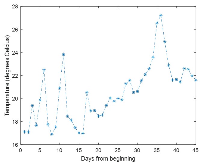
Another weakness of the current version of the manuscript is the use of a supposed "contradiction" in the existing literature to create the context for the present study. Although the various studies cited do have many differences in their results, those other papers lay out many nuanced hypotheses for those differences. Almost none of the studies cited in this manuscript actually reported blanket increases or decreases in urban birds, as suggested here, and each of those papers includes examples of species that showed different responses. To suggest that they are on opposite sides of a supposed dichotomy is a misrepresentation. Many of those other studies also included a larger number of different species, whereas this study focused on three. Finally, this study was completed at a much finer spatial scale than most others and was examining micro-habitat differences rather than patterns apparent across landscapes. I believe that highlighting differences in scale to explain nuanced differences among studies is a much better approach that more accurately adds to the body of literature.
We thank the reviewer for this good feedback and revised the manuscript, accordingly, placing more emphasis on the micro-scale of this study.
Finally a note on L244-247: I would recommend against discounting the possibility that lockdowns resulted in changes to the birds' vocal acoustics, as Derryberry et al. 2020 found, especially while suggesting that their results were the effects of signal processing artifacts. Audio analysis is not my area of expertise, but isn't it possible that the birds did increase call intensity, but were simply not willing (or able) to increase it to the same degree as the additional ambient noise?
This is an important question. The fact is that when ambient noise increases (at the relevant frequency channels), then the measured vocalizations will also increase. There is no way to separate the two effects. Thus, as scientists, when we cannot measure an effect, it is safer not to suggest an effect. Unfortunately, most studies that claim an increase in vocalizations’ intensity in noise, do not account for this potential artifact (and most of them do not estimate noise at a species-specific level as we have done). This has created a lot of “noise” in the field. We do not want to criticize the Derryberry results without analyzing the data, but from reading their methods it does not seem like they took the noise into account in their acoustic measurements. But if you look at their figure 4A you will see a lot of variability in measuring the minimum frequency – which could be strongly affected by ambient noise.
In light of the above, we thus prefer to be careful and not to state changes that are probably false. We added some of this information to the manuscript. We also added the linear equations to the graph (in the caption of figure 3) where it can be seen that the slope is always <=1.
Reviewer 2:
The explanation of methods can be improved. For example, it is not clear if data were low-pass filtered before resampling to avoid aliasing.
We edited the methods and hopefully they are clearer now. Regarding the specific question – yes, an LPF was applied to prevent aliasing before the resampling. This information was added to the manuscript.
It is quite possible that birds move into the trees and further from the recorders with human activity. Since sound level decreases by the square of the distance of the source from the recorders, this could significantly affect the data. As indicated in the Discussion, this is a significant parameter that could not be controlled.
The reviewer is correct, and we addressed this point. Such biases could arise with any type of surveying including manual transects (except for perhaps, placing tags on the animals). We note that we only analyzed high SNR signals and that the species we selected somewhat overcome this bias – both crows and parakeets are not shy and Prinias are anyway shy and prefer to not be out in the open. We would also expect to see a stronger effect for human speech if this was a central phenomenon, and we did not see this, but of course this might have affected our results.
In interpreting the data, the authors mention the effect of human activity on bird vocalizations in the context of inter-species predator-prey interactions; however, the presence of humans could also modify intraspecies interactions by acting as triggers for communication of warning and alarm, and/or food calls (as may sometimes be the case) to conspecifics. Along the same lines, it is important to have a better understanding of the behavioral significance of the syllables used to monitor animal activity in the present study.
We agree with this point and added more discussion of both this potential bias and the type of syllables that were analyzed.
Another potential effect that may influence the results but is difficult to study, relates to the examination of vocalizations near to the ambient noise level. This is the bandwidth of sound levels where most significant changes may occur, for example, due to the Lombard effect demonstrated in bird and bat species. However, as indicated, these are also more difficult to track and quantify. Moreover, human generated noise, other than speech, may be a more relevant factor in influencing acoustic activity of different bird species. Speech, per se, similar to the vocalizations of many other species, may simply enrich the acoustic environment so that the effects observed in the present study may be transient without significant long-term consequences.
We note that we already included a noise parameter (in addition to human speech) in the original manuscript. Following the reviewer’s comment, we examined another factor, namely we replaced the previous ambient noise parameter with an estimate of ambient noise under 1kHz which should reflect most anthropogenic noise (not restricted to human speech). This model gave very similar results to the previous one (which is not very surprising as noise is usually correlated). We added this information to the revised manuscript, and we now also added examples of anthropogenic noise to the supplementary materials (Fig. S8). In general, we accept the comments made by the reviewer, but would like to emphasize that we only analyze high SNR vocalization (and not vocalizations that were close to the noise level). This strategy should have overcome biases that resulted from slight changes in ambient noise.
In general, the authors achieved their aim of illustrating the complexity of the effect of human activity on animal behavior. At the same time, their study also made it clear that estimating such effects is not simple given the dynamics of animal behavior. For example, seasonality, temperature changes, animal migration and movement, as well as interspecies interactions, such as related to predator-prey behavior, and inter/intra-species competition in other respects can all play into site-specific changes in the vocal activity of a particular species.
We completely agree and tried to further emphasize this in the revised manuscript. This is one of the main conclusions of this study – we should be careful when reaching conclusions.
Although the methods used in the present study are statistically rigorous, a multivariate approach and visualization techniques afforded by principal components analysis and multidimensional scaling methods may be more effective in communicating the overall results.
Following this comment, we ran a discriminant function analysis with the parameters of the best model (site category, ambient noise, human activity, temperature and lockdown state) with the task of classifying the level of bird activity. The DFA analysis managed to classify activity significantly above chance and the weights of the parameters revealed some insight about their relative importance. We added this information to the revised manuscript
Suggestions for improvement:
In Figure 2, the labeling of the Y-axis in the right panel should be moved to the left, similar to A and C. This will provide clear separation between the two side-to-side panels.
Revised
In Figure 3, it will be good to see the regression lines (as dashed lines) separately for the lockdown and no-lockdown conditions in addition to the overall effect.
Revised
Editor:
Limitations
Scale: The study's limited spatial and temporal scale was not addressed by the authors, which contrasts with the broader scope of other cited studies. To enhance the significance of the study, acknowledging and clearly highlighting this limitation, along with its potential caveats, modifications in the language used throughout the text would be beneficial. Furthermore, although the authors examined slight variations in habitat, it is important to note that all sites were primarily located within an urban landscape.
We revised the manuscript accordingly.
Control period: The control period is significantly shorter than the lockdown treatment period and occurs at a different time of year, potentially impacting the vocalization patterns of birds due to different annual cycle stages. It is crucial to consider that the control period falls within the pandemic timeframe despite being shortly after the lockdowns ended.
Revised – we included a control comparison to periods of equal length within the lockdown. People gradually stopped obeying the lockdown regulations before its removal so in fact, the official removal date is probably an overestimate for the effect of the lockdown. We now explain this.
Recommendations
Human-generated noise, beyond speech, might have a greater influence on the acoustic activity of various bird species, but previous studies lacked detailed human activity data. Instead of solely noting the number of human talkers, the authors could quantify other aspects of human activity such as vehicles or overall anthropogenic noise volume. Exploring the relationships between these factors and bird activity at a fine scale, while disentangling them from bird detection, would be compelling. It is important to consider the potential difficulty in resolving other anthropogenic sounds within a specific bandwidth, which could be demonstrated to readers through spectrograms and potential post-pandemic changes. Such information, including daily coefficient of variation/fluctuation rather than absolute frequency spectra, could provide valuable insights.
We note that we have already included an ambient noise factor (in addition to human speech) in the previous version. Following the reviewers’ comments, we examined another factor, namely we replaced the current ambient noise parameter with the ambient noise under 1kHz which should reflect most of anthropogenic noise (not restricted to human speech). This model gave very similar results to the previous one (which is not surprising as noise is usually correlated). We also added several spectrograms in the Supplementary material that show examples of different types of noise.
Authors should limit their data interpretation to the impact of lockdown on behavioral responses within small-scale variations in habitat. A key critique is the assumption that activity changes solely resulted from the lockdown, disregarding other environmental factors and phenology.
Following the editor comment we realized that our conclusion\assertations were not clear. We never claimed that activity changes solely resulted from the lockdown. While revsing the mansucirpt we ensurred that we show a significant effect of temperature, ambient noise and human activity – all of which are not dependent on lockdown. We made an effort to emphasize the complexity of the system. We show that the lockdown seemed to have an additional impact, but we never claimed it was the only factor.
To address this, the authors could compare acoustic monitoring data within a shorter timeframe before and after the lockdown (20 days), while also controlling for temperature effects, to strengthen the validity of their claims. They would need to explain in their discussion, however, that such a comparison may still be confounded by any carry-over effects from the 10 days of treatment.
This analysis would be difficult because although the lockdown was officially removed at a specific date, it was gradually less respected by the citizens and thus the last period of the lockdown was somewhere between lockdown and no-lockdown. This is why we chose the approach of taking 10 days randomly from within the lockdown period and comparing them with the 10 post-lockdown days. We now clarify the reason better.
An option is that authors could frame their analysis as a study of the behavior of wildlife coming out of a lockdown, to draw a distinction from other studies that compared pre-pandemic data to pandemic data.
Good idea – revised.