Do these AI-related business growth things include replacing workers with machines?

The OOHC Toolbox source helped me understand public shaming differently. It explains that shame can make a person feel like their whole self is bad, while guilt focuses on a specific behavior. This connects to online shaming because public criticism often attacks someone’s identity instead of helping them repair harm.

I chose this source because it shows why shame can sometimes be seen as useful, especially when weaker groups are trying to pressure more powerful people. But it also seems risky, because public shaming can easily become excessive. That connects well to this chapter’s distinction between public criticism and public shaming.

This article discusses the concept of shame, specifically in relation to child development. It explains how shame is, in many ways, necessary for children to experience as it discourages them from harmful behaviors. However, the article also notes that in the context of abuse and trauma, shame can be very harmful, leading to lifelong scars for the child.

I read this article which discussed the effects of pranks similar to the one shown/done by Jimmy Kimmel. The author talks about how jokes like the Halloween candy one are actually harmful to children as their humor is not developed enough to understand the humor in the situation afterwards. While the prank is not something that should cause psychological trauma (as the situation is made better by the truth afterwards), it is still harmful for children to face such negative emotions from a trusted figure.

The article argues that Jimmy Kimmel’s Halloween candy prank is not harmless fun for young kids, but confusing and emotionally upsetting because they take the lie literally and feel real betrayal. The psychologist notes that children under about 10 don’t share adults’ sense of humor, so they can’t easily see it as a joke. He also says it’s usually not “trauma” in the clinical sense, since the parent quickly reveals the truth, but it still shows poor judgment to turn a child’s distress into entertainment.

I think the chapter shows why public shaming is ethically complicated. Online criticism can hold people accountable, but it can also become punishment without context, forgiveness, or a chance to change. I like the idea of a retract feature because people should be able to admit mistakes and repair harm, not be permanently defined by one post.

Fred Trotter (me) analysis of the security of Fax from 2010

Change indicating that digital copies of patient records stored in the memory of fax machines was covered under HIPAA

Discussing print then scan-over-fax

Transparent Peer Review

Download the complete Review Process [PDF] including:

• reviews
• authors' reply
• editorial decisions

</br>

I like this point because “cancel culture” has become such a vague term. People use it to describe a lot of very different situations, from serious accountability to just being criticized online. Breaking it into public shaming and public criticism feels clearer and more useful.

The most important factors in making public shaming bad is proportionality and evidentiality, in my opinion: often, public shaming escalates far beyond what is warranted. I often see on Twitter that the escalating event is just a difference in media opinion (and not one based on anything substantial). Evidentiality is one factor because it's often the case that acts/words that are put upon a person are often highly exaggerated or sometimes even fabricated- which leads to a huge deal of drama for often no reason at all.

Even if this article is meant to be satirical. I do see a sense of truth in this, just from my personal perspective gained from other people's social media use. When I read this section, it made me immediately think of people who "hate" certain celebrities. I often encounter people who make it very known they dislike certain public figures for their "recent scandals" and affairs, that it just seems like another form of being parasocial. I understand if this hate comes from a celebrity doing actual wrong doings, but I am more specifically referring to people who hate celebrities for petty drama/news. For example, it seems like a big personality trait is to hate on Chappel Roan for her online drama, yet it seems they only tune in for the entertainment of it all, not actually because she is really doing anything noteworthy. I say this as someone who has no regard or care for her at all, because from an outside perspective, some people's hatred of celebrities seems to stem from the entertainment they get from it.

Government forces used violence to stop the labor protests, showing how authorities often sided with businesses against striking workers during labor conflicts.

The strikes became a major conflict between the working class and wealthy business owners, showing deep economic and social divisions during the Gilded Age.

In my opinion I think destroying things is never the answer

State governments used military force to stop the strikes and protect businesses.

important

interesting paper. since the two strains are foundational to the study, need more information on them. for strain RM1164, only says who donated it. need how isolated, where isolated, when, etc. for strain HC1, again, just gives source. need relevant patient data, history, date of isolation, method, etc.

delete

delete

BOLD

BOLD

delete

delete

delete and capitalize the E in educators

delete and capitalize the E in educators

delete and capitalize the E in educators

delete

delete

delete section it is repeated 4.3

delete question #7

under these two bullets add the following: What strengths-based strategies from the case could be applied to multilingual learners in K–12 classrooms?

Where do you see opportunities to improve?

delete and replace with: an

Delete this entire section it is a repeat from begining of 1.4.

Hello, Could you please update this preprint as the final version of this work is published now: https://www.nature.com/articles/s41598-026-37259-7

Gesell held the belief that genes were responsible for the development of a child. He actively opposed efforts to teach children. His reasoning for this was that he believed that children would naturally begin engaging in behaviors once their systems sufficiently matured.

Jean-Jacques Rousseau believed that children should be allowed their own ways of thinking, arguing that they had a biological timetable but were not little adults.

Biological maturation was monumental to terming Rousseau as the father of developmental psychology.

Antonio Rotta (1828–1903) Il Ciabattino (At the Cobbler's Workshop)

Major theme of this text is mental health and loss of identity

The man collapsed while the narrator continues moving

Yellow may be the color used to describe sickness

The house may be viewed as a prison

Is John dismissive of the narrators feelings or emotions?

I'm struggling to work through the model of cytoplasmic organization and how that translates to disease pathogenesis. Is the hypothesis that this organization is mostly a result of disrupted cytoskeletal structure, so that the cell can't transmit forces as well? Or does crowding also play a role in this physical aspect of the cell?

I'm curious if reduced ribosome production has any impact on total protein levels within the cell, or if it just impacts cytoplasmic organization?

Do you have a sense (on the molecular level) of what these two classes represent? Or how you conceptualize these two classes of proteins based on what their functions might be within a cell?

大多数人认为GPU编译器已经提供了足够的优化选项，开发者可以通过手动调整获得最佳性能。但作者指出，在当前AI基础设施的竞争环境下，这种观点已经过时，暗示传统方法无法满足现代AI工作负载的性能需求。

大多数人认为一旦开发者完成优化工作，就没有更多性能提升空间。但作者表明，即使是"完成"的优化代码仍可能通过编译器级别的调整获得显著提升（高达15%），这挑战了开发者对优化极限的认知。

大多数人可能认为AI驱动的自动调优工具可以弥补代码质量不足的问题，但作者明确表示，即使是CompileIQ这样的先进工具也需要基于已经相当优化的代码才能发挥最大作用。这挑战了"自动化工具可以解决一切性能问题"的常见误解。

大多数人认为优化整个应用程序或算法才能获得显著性能提升，但作者指出，仅仅优化占计算量90%的两个关键内核类型就能带来最大收益。这与广泛应用的"全面优化"策略相悖，暗示开发者应该将资源集中在最关键的代码路径上。

大多数人认为编译器已经提供了足够的优化，开发者只需关注算法和代码实现即可。但作者认为，即使是最先进的GPU编译器也使用通用的启发式方法，这些方法无法针对特定工作负载进行优化，导致性能损失。这挑战了开发者社区对编译器优化能力的普遍认知。

大多数人认为历史经验可以预测AI对就业的影响，但作者认为这次可能真的不同，AI可能以前所未有的方式吞噬工作。这一观点挑战了技术变革历史模式的适用性，暗示AI可能是真正的范式转变。

大多数人认为计算机科学和编程技能仍然是就业的保证，但作者认为这些技能可能不再是工作的保证，这解释了计算机科学专业人数的下降。这一观点挑战了传统技术教育价值的认知，暗示AI正在改变就业市场的基本规则。

大多数人认为AI会压低工资或导致工资增长停滞，但作者认为AI高度影响行业的工资实际上在快速增长。这一发现与主流预期相悖，表明AI可能正在增加而非减少高技能工作的价值。

大多数人认为AI会替代所有相关工作，但作者认为AI对就业的影响取决于使用方式——完全自动化的工作确实减少，但增强人类工作的AI反而促进了就业增长。这一区分挑战了AI必然导致失业的简单化观点。

大多数人认为合规风险主要来自人类行为者和交易对手。但作者认为随着AI代理成为网络上的主要购买者，将出现全新的风险类别。这挑战了传统合规框架的基本假设，暗示未来合规需要考虑非人类行为者的独特风险特征。

大多数人认为合规工作是枯燥且增长缓慢的辅助职能，但作者认为合规已成为美国增长最快的职业之一，仅次于美甲师。这挑战了人们对合规工作价值的传统认知，暗示合规职能在当代经济中扮演着比想象中重要得多的角色。

大多数人认为复杂的AI系统漏洞需要复杂的攻击手段，但作者认为这个漏洞仅通过修改HTTP主机头就能实现，这挑战了'高级系统需要高级攻击'的直觉认知，展示了简单输入验证错误可能导致灾难性后果的反直觉案例。

大多数人认为开源软件的安全风险主要来自小众或使用率低的项目，但作者认为即使是像Starlette这样每周下载量高达3.25亿次的主流开源框架也可能存在严重漏洞，这挑战了'流行项目更安全'的普遍认知。

This talks about how you pick the person you are going to be with in life and who you are going to reproduce with and all of the things that come with that.

In summary it talks about how your family shapes you into the community and your personality and how you treat people.

Emotional support is basically it deals with relationships and the emotional that tie into that when having a partner.

Economic support is the basic need in life to get by like food, shelter, and clothes and in Many different countries they do it differently in some ways but it all comes done to food,shelter,clothes at the end of the day.

• A study published by the American Psychological Association found that walking consistently boosts creative thinking compared to sitting or being pushed in a wheelchair.
• Walking improved performance on tests measuring divergent thinking—such as coming up with alternate uses for common objects and original analogies—but walkers fell slightly behind seated participants when solving problems with a single correct answer (convergent thinking).
• In the experiments, an overwhelming majority of participants (81% to 100% depending on the specific group) generated significantly more creative and novel responses while walking.
• The creative boost was found to be a result of the physical act of walking itself rather than the outdoor environment, as walking indoors on a treadmill yielded similar strong improvements in creative output.
• The study revealed a residual effect of physical activity, showing that participants continued to display higher levels of creative inspiration even after they sat back down following a walk.

Hacker News Discussion

• Users widely agreed with the study, sharing personal anecdotes about solving complex programming or engineering problems only after stepping away for a walk.
• Many comments criticized modern corporate management for prioritizing rigid quantitative metrics—like "seats in butts" or hours worked—instead of allowing employees to take walks, which would ultimately optimize productivity and happiness.
• Some users suggested integrating short, frequent physical activities or exercise sessions directly into the workday rather than rigidly separating fitness from working hours.
• A few participants looked at the topic through an evolutionary lens, speculating that the human brain and cognitive processes naturally evolved to function optimally alongside bipedal locomotion, since endurance hunting required multitasking and complex reasoning while moving.

I wonder what the average time was to build these? If im correct, Egypt built their pyramids very fast.

Its interesting how every religion is different and how they work.

bars

gold

new social patterns

Hello Class. Hypothesis allow us to interact in this youtube video as if it were a mini social network. Respond to this post by leaving your impressions about the content of this video. Leave three major takeaway for you and screenshot your contribution. Everyone should respond to this thread. Let me kow if you have any questions.

look up this artist - what is your interpretation of this scene? what formal techniques are employed to achieve this vision/intention? do research on the cultural and socio-policital climate of this era, what was the pre-dominant subject of this artist's paintings and how did the subject matter/technique/medium, etc. evolve (or not evolve?) , identify why this painting is relevant to the conversation of "awe" and "absurdity"

https://en.wikipedia.org/wiki/Stand_by_Me_(Charles_Albert_Tindley_song)

See also:<br /> - "Stand By Me Father" - The Soul Stirrers https://www.youtube.com/watch?v=weYZt3FAqi4

via u/ksigler at https://www.reddit.com/r/typewriters/comments/1t5resr/replacement_feet_for_a_hermes_rocketbaby/

very important

important

very important

important

important

important

super important

Maxim Suravegin is working on a Ph.D. thesis relating to typewriters.<br /> https://www.facebook.com/groups/TypewriterCollectors/posts/10163573420424678/

The solutions from one generation can often be passed down to newer generations for intergenerational use.

We change in the physical, cognitive, and psychosocial domains. They each pertain to physical capabilities, changes in intelligence and mental skills, and growth in emotional intelligence, conjointly with relationships in one's life, each respective to their own kinds of intelligence.

Development doesn't stop at the age of 25. We are always changing and growing, even when society may tell us otherwise.

eLife Assessment

The nematode C. elegans is an ideal model in which to achieve the ambitious goal of a genome-wide atlas of protein expression and localization. In this paper, the authors develop a rational and useful strategy for at-scale tagging of all protein coding genes with fluorescent markers, providing solid evidence that it could be a feasible foundation for a large-scale, community-wide project.

Reviewer #1 (Public review):

Summary:

Eroglu and Hobert demonstrate that injecting CRISPR guides and repair constructs to target three genes at a time, tagging each with a different fluorescent protein, and selecting which gene to tag with which fluorophore based on genes' expression levels, can improve efficiency of gene tagging.

Strengths:

This manuscript demonstrates that three genes can be targeted efficiently with three different fluorophores. It also presents some practical considerations, like using the fluorophore least complicated by agar/worm autofluorescence for genes with low expression levels, and cost calculations if the same methods were used on all genes.

Weaknesses:

Eroglu has demonstrated in a previous publication that single-stranded DNA injection can increase efficiency of CRISPR in C. elegans, while inserting two fluorescent proteins and a co-CRISPR marker into three loci, and Paix et al 2015 demonstrated simultaneous insertion of two fluorescent tags. The current work is valuable and incremental advance. In general, I applaud the authors' willingness to strategize about how whole proteome tagging might be accomplished. I predict that the advance here will be one of many small advances that will get the field to that goal. The title oversells the advance presented, in my view, since seems like one among many key advances, and the first sentence of the Discussion seems a more apt summary of the key advance here.

Some injections targeted genes on the same chromosome together, which will create unnecessary issues when doing crossing that will be useful for some future experiments. This made me wonder if injecting 3 together really is helpful vs targeting each gene separately, since only 5 worms need to be injected. It cuts time down by 2/3, but perhaps avoiding targeting the same chromosome with two tags would be useful.

The limited utility of current blue fluorescent proteins makes me wonder if it's worth using at this stage, before there are better blue fluorescent proteins, or better yet, far red, to avoid issues with live imaging under phototoxic UV or near-UV illumination.

Reviewer #2 (Public review):

Original Review:

The manuscript by Eroglu and Hobert presents a set of strains each harboring up to three fluorescently tagged endogenous proteins. While there is technically nothing wrong with the method and the images are beautiful, we struggled to appreciate the advance of this work - who is this paper for?

As a technical method, the advance is minimal since the first author had already demonstrated that three mutations (fluorophore insertion and co-CRISPR marker) could be introduced simultaneously.

As a pilot for creating genome-scale resources, it is not clear whether three different fluorophores in one animal, while elegantly designed and implemented, will be desired by the broader community.

Finally, the interpretation of the patterns observed in the created lines leaves much to be desired. A Table with all the observations must be included and can replace the tedious (and often wrong) descriptions of the observations with the different lines. It would be too much to point out every mistaken expectation of protein expression. Two examples include:

The expectation that ACDH-10 is enriched in the intestine and epidermal tissues (hypodermis) is naïve - there are multiple paralogs of this protein (look at WormPaths or WormFlux) that may share functions in different tissues. There is also no reason to assume that fatty acid metabolism does not occur in other tissues (including the germline). Finally, there are no published studies about this enzyme, so we really don't know for sure what it's doing.

The expectation that HXK-1 is ubiquitously expressed is similarly naïve. There are three paralogous enzymes that are all associated with the same reaction, and we have shown that these three function redundantly in vivo, perhaps in different tissues (PMID: 40011787). Moreover, single cell RNA-seq data (PMID: 38816550) also shows enrichment of hxk-1 in gonadal sheath cells.

The table should have at least the following information: gene/protein name - Wormbase ID - TPM levels of single cell data assigned to tissues for L2, L4 and adult (all published) - tissues in which expression is observed in the lines presented by the authors.

Other points:

(1) We would encourage the authors to provide systematic validation of the reported insertions. The manuscript reports that 24 of 30 tags were isolated and visible but does not clearly state whether each isolated line was confirmed by sequence‑level validation to be correctly in‑frame and free of unintended mutations at the target locus.

(2) The manuscript presents aggregated success counts (e.g., 8/10 mTagBFP2 tags, 9/10 mStayGold, 7/10 mScarlet3) and useful narrative descriptions of injection outcomes. We suggest also to include per‑locus success rates.

(3) For pools that required re‑injection after initial failures, we would like to see a description of the specific changes that were made to the injection mixes or procedures (e.g., new repair template prep, different Cas9 reagent lot, guide redesign). This will be useful troubleshooting information for others.

(4) The authors states that the fluorophore sequences are codon-optimized for C. elegans. We suggest they provide the exact donor/tag sequences used specifically state whether the fluorophore sequences contain any synthetic/artificial introns or other sequence modifications (e.g., silent PAM‑disrupting mutations) were included in the donor templates.

(5) Page 3: Include a reference for "The C. elegans genome encodes around 20,000 genes"

We hope these comments are useful.

Comments on Revised Version:

Overall, we found the responses to be quite recalcitrant.

We have one remaining composite concern about the comparison between observed expression patterns with the new strains versus published data.

First, the authors only report patterns for one stage while it should be not too much effort to image the different life stages. However, since this is a revision, we are not formally requesting they do this.

Second, in the now provided Table (thank you) 'observed expression' (last column) is lacking for 9 of the 30 proteins, and for 6 of these the procedure was not successful. Why not report patterns for the other three? It is confusing also because on page 5, the authors say that "overall, 24 of 30 tags ...all of which were visible with fluorescence stereomicroscopy" - are we missing something? Also, they then said that they "obtained 6/9 of the originally failed tags"; why are the corresponding patterns not included in table 1, and are 9 proteins still labeled as "no" in the "success?" Column?

Third, we strongly feel that the response to our comments about expression patterns is not adequate. On page 5 the authors say that "all proteins were expected to be ubiquitously expressed" and that "scRNA-seq indicated that transcript abundance was ubiquitous and without strong tissue-specific enrichment with few exceptions". However, in their rebuttal, the authors now argue for tissue-specific expression for proteins with paralogs, turning around their own argument! Moreover, their Table indicates that many genes show tissue-enriched expression by RNA-seq while many of their tagged proteins exhibit ubiquitous expression.

Overall, this indicates that both the overall accomplishment of generating tagged protein strains and analyzing their expression is oversold.

Reviewer #3 (Public review):

Summary:

The authors argue that establishing the expression pattern and sub-cellular localisation of an animal's proteome will highlight hypotheses for further study. This claim is probably accepted by many in the community. This manuscript seeks to confirm the feasibility of establishing such a resource, by using current transgenic methods to knock in DNA encoding different colored fluorescent tags into C. elegans genes.

Strengths:

The authors make the points above. For example, they provide evidence that the C. elegans germline harbors two populations of mitochondria that differ qualitatively in the proteins they express. They also confirm that labelling the whole proteome is an achievable goal with relatively limited resources and time.

Weaknesses:

The work is somewhat incremental in that it uses existing transgenic technology. Cell biology in C. elegans is challenging because of the small size of many of its cells, notably neurons. This can make establishing the sub-cellular localisation of a fluorescently tagged protein, or co-localizing it with another protein, tricky. The authors point out in their introduction that advances in light microscopy such as diSPIM, STED and ISM (a close relative of SIM), have increased the resolution of light microscopy. They also point out that recent advances in expansion microscopy can similarly help overcome the resolution limit. However, they do not use these technologies to characterize their transgenic strains.

Reviewer #4 (Public review):

Summary:

Tagging the entire proteome of a metazoan would be a landmark achievement, providing a powerful complement and extension to existing "omic" catalogs in model systems. Here, Eroglu and Hobert argue that efficiently tagging multiple loci in a single "batch" would make the community-based achievement of this goal realistic. They provide rigorous evidence that such an approach is indeed feasible, exploring issues related to efficiency, design and screening strategies, disruption of gene function, and the potential for endogenously tagged alleles to reveal unexpected aspects of protein expression and localization. While the work has some minor gaps that are important to rigorously assess the feasibility of the proposed effort, the detailed and valuable insights that emerge should provide impetus to the community to coordinate efforts to make this ambitious goal a reality.

Strengths:

The work has numerous strengths. The authors provide compelling evidence that:

- three distinct loci can be efficiently targeted with three distinct fluorescent tags in a single injection.

- thoughtful targeting design can reduce the likelihood of disruption of function by the tag.

- systematic design principles based on expression level and predicted localization/function can be used to optimize tagging strategies.

- the resulting tags can provide unexpected insight into patterns of protein production and subcellular localization.

Not all of these advances are novel in themselves, but taken together, they represent an important technical and conceptual advance. The most important strength comes from the exceptionally high value of the goal itself, in that the work is that it has the potential to spur a community-wide effort toward achieving the ambitious goal of proteome-wide tagging.

Weaknesses:

The work's shortcomings are minor.

- One concern has to do with the feasibility of the proposed screening strategies. The experimental design cleverly coinjects tags for three loci in different gene expression 'zones'; this expression level determines which tag will be used. As the authors allude to, there is an important distinction between genes with the same overall FKPM value between those that are expressed broadly and those focally expressed in a specific tissue. The proposed strategy claims that there are a sufficient number of highly expressed genes "to be used as visible markers" for recovering successfully edited animals. It would be useful for the authors to discuss the issue of broad vs focused expression among this set of genes a bit more thoroughly, with an eye toward the issue of how likely it is that these genes could indeed consistently be used as visible markers, particularly for those at the low end of this limit.

- What fraction of the proteome (on a per-gene basis) is secreted proteins? How difficult will it be to screen these for successful tags? Are there specific tags that would be more optimal for secreted proteins? (The authors mention the use of an SL2 or T2A cassette to label the cells in which these proteins are expressed but note that there are technical challenges associated with doing this at scale.)

- For secreted and/or weakly expressed genes, it would be useful for the authors to estimate for what fraction of these would successful insertions need to be screened by PCR, and what resources (time and money) this would likely entail.

- For how many genes would a single tag not capture all predicted isoforms?

- Finally, some readers might object to the authors' assertion in the abstract that this work is "a first step in this direction" (presumably referring to designing a strategy for whole-proteome tagging). There is no concern that the authors are disregarding the extensive work of other groups, as they explicitly mention the contributions of other groups to the foundation that enables the present work. However, the spirit of the abstract could be misinterpreted by a well-intentioned reader.

Author response:

The following is the authors’ response to the original reviews.

eLife Assessment

The nematode C. elegans is an ideal model in which to achieve the ambitious goal of a genome-wide atlas of protein expression and localization. In this paper, the authors explore the utility of a new and efficient method for labeling proteins with fluorescent tags, evaluating its potential to be the basis for a larger, genome-wide effort that is likely to be very useful for the community. While the evidence for the method itself is solid, carrying out this project at a large scale will require significant additional feasibility studies.

We appreciate the editor’s recognition that the evidence for our method is solid and that a genome-wide protein atlas in C. elegans would be highly valuable to the community. However, we respectfully disagree that “significant additional feasibility studies” are required. Take the yeast proteome-wide GFP tagging project (Huh et al., Nature 2003). It achieved ~75% coverage of ~6,000 proteins directly from an established protocol without any prior significant feasibility studies, at least to our knowledge. While the C. elegans genome is 3 times in size, we would argue that our tagging protocol may even be less labor intensive as it does not involve any cloning and the screening is visual, requiring no molecular biology skills. Reviewer 3 notes: ‘They also provide convincing evidence that labelling the whole proteome is an achievable goal with relatively limited resources and time.’

Our pilot study validates all key parameters for genome-wide scaling: editing efficiency at novel loci with untested reagents, viability of tagged worms, and detectability of multiple spectrally separated fluorophores across expression ranges. These address the core technical, biological, and practical challenges of large-scale endogenous tagging in a multicellular organism, leaving no fundamental barriers in our view.

The proposed cost and timeline align quite favorably with established large-scale consortium projects: e.g., ENCODE pilot analyzed 1% of the human genome at ~$55 million over 4 years; Mouse Knockout Consortium scaled to ~20,000 genes over 20 years (ongoing) with ~$100 million; Human Protein Atlas mapped ~87% of proteins with antibodies in fixed cells (through much more labor intensive methods) over 20+ years at >$100 million. With ~8% of C. elegans genes already tagged (WormTagDB) and labs already tagging entire gene classes (PMID: 40463100), scaling our protocol to the proteome is feasible, potentially covering the genome in 5-6 years by a single lab or faster with distributed effort at a reagent cost of merely $2.2 million. The main barriers now are funding commitment and assembling collaborators, not further feasibility testing.

Public Reviews:

Reviewer #1 (Public review):

Summary:

Eroglu and Hobert demonstrate that injecting CRISPR guides and repair constructs to target three genes at a time, tagging each with a different fluorescent protein, and selecting which gene to tag with which fluorophore based on genes' expression levels, can improve the efficiency of gene tagging.

Strengths:

This manuscript demonstrates that three genes can be targeted efficiently with three different fluorophores. It also presents some practical considerations, like using the fluorophore least complicated by agar/worm autofluorescence for genes with low expression levels, and cost calculations if the same methods were used on all genes.

Weaknesses:

Eroglu has demonstrated in a previous publication that single-stranded DNA injection can increase the efficiency of CRISPR in C. elegans while inserting two fluorescent proteins and a co-CRISPR marker into three loci. The current work is, therefore, an incremental advance. In general, I applaud the authors' willingness to think ahead to how whole proteome tagging might be accomplished, but I predict that the advance here will be one of many small advances that will get the field to that goal.

Our manuscript indeed builds on prior multiplex editing (including our own co-CRISPR work), but the manuscript's primary contribution is not a novel technical breakthrough per se. Instead, our main goal was to pilot and strategize a feasible path to whole-proteome tagging in C. elegans and, most critically, test the following key parameters: (1) success rate of triple pools with prior untested reagents at novel targets; (2) utility of fluorophores across expression levels; (3) major effects on tagged protein function. In prior multiplexing, we used two targets which we already knew could be edited quite efficiently, with the 3rd target a point mutation with nearly 100% efficiency. Thus, it was not at all clear that picking 3 random genes and replacing the 3rd highly efficient locus with another less efficient large insertion would work or be sufficiently scalable for thousands of novel genes with unvalidated reagents at first pass.

The title vastly oversells the advance in my view, and the first sentence of the Discussion seems a more apt summary of the key advance here.

Some injections target genes on the same chromosome together, which will create unnecessary issues when doing necessary backcrossing, especially if the mutation rate is increased by CRISPR.

We disagree with the reviewer’s assessment of the need for backcrossing, for two reasons: (1) Prior studies have shown that off-target mutations are not a serious concern in C. elegans (reviewed in PMID: 26336798). For instance, WGS of strains after CRISPR/Cas9 found negligible off-target effects (PMID: 25249454, PMID: 30420468 – using similar RNP/ssDNA method and multiple guides; PMID: 23979577, PMID: 27650892 using other methods). Targeted sequencing studies have reported similar findings, using various CRISPR/Cas9 methods, with essentially no mutations at sites other than the intended target (PMID: 23995389; PMID: 23817069). (2) If the goal is to tag the entire genome, the introduction of backcrossing should not reasonably be a routine part of the initial tagging.

Lastly, if one really does want to backcross, the existence of tags on the same chromosome is actually an advantage because it permits selection for recombinants with wild-type chromosomes.

Also, the need for backcrossing and perhaps sequencing made me wonder if injecting 3 together really is helpful vs targeting each gene separately, since only 5 worms need to be injected.

Apart from our disagreement regarding backcrossing, we are puzzled by the reviewer’s comment. Why would one do single tagging at a time, rather than triple tagging if the whole point is to scale up tagging? It is important to keep in mind that the rate limiting step for tagging the whole genome is the number of injections that can be done per day. Since there is no cloning to generate the repair templates/guides and all other reagents are commercially available and not sample specific, these can be prepared quite rapidly. Being able to isolate multiple lines (together or independently) from the same injection increases throughput 3-fold and in our view does not provide any disadvantages as individual tags can be isolated independently if desired.

Beyond the numerous technical advantages pooling provides (also lower cost and throughput for making injection mixes as well as imaging), our results show that it yields epistemic benefits as well: we would never have noted the subcellular pattern in Fig. 6B, C with different sets of mitochondria being marked by different mitochondrial proteins had we imaged them separately or even aligned to a pan-mitochondrial landmark. As we mentioned in the discussion, grouping proteins predicted to localize to the same compartment together can simultaneously test how uniform or differentiated such compartments are during the screen.

The limited utility of current blue fluorescent proteins makes me wonder if it's worth using at all at this stage, before there are better blue (or far red) fluorescent proteins.

We do not think that the utility of current BFPs is that limiting. At least the theoretical brightness of mTagBFP2 is comparable to that of EGFP (PMID: 30886412), which was useful for the bulk of currently tagged proteins. Due to modestly higher autofluorescence in the blue spectrum, the practical brightness is somewhat less ideal, but we have shown that many proteins are expressed high enough to be detected quite well with mTagBFP2 by eye at low magnification. We also note that many tags that are not visible by eye under a dissection scope become visible with long exposure cameras of widefield microscopes or modern confocal (GaAsP) detectors, so the list of genes detectable with mTagBFP2 is likely to be much higher. We routinely use mTagBFP2 to super-resolve subnuclear structures with endogenous tags (e.g., in the nucleolus), with some tags having lower annotated FPKMs than the genes tested here.

Some literature reviews, particularly in the Introduction and Abstract, rely too much on recent examples from the authors' laboratory instead of presenting the state of the field. I'd like to have known what exactly has been done with simultaneous injection targeting multiple loci more thoroughly, comparing what has been accomplished to date by various laboratories' advances to date.

We are not sure what the reviewer is referring to. In the Abstract, we do not refer to any literature. In the Introduction, we cite 28 papers, 6 of those from our lab (4 of which providing examples of protein tags). We do not believe that this can be fairly called an unbalanced presentation of the state of the field.

This being said, we have gladly expanded our Introduction to provide more background on co-CRISPRing. Labs have routinely used co-conversion (“coCRISPR”) markers for picking out their intended edits (e.g., point mutations or insertions), as it has been shown by multiple groups that a CRISPR/Cas9 edit at one locus correlates with efficiency at other simultaneous targets (PMID: 25161212). Generally, making point mutations with the Cas9/RNP protocol is highly efficient, especially at specific loci such as dpy-10. However, multiple FP-sized insertions have not been routinely attempted. We and only one other group have successfully attempted it using previously working targets and reagents (e.g., 28% in PMID: 26187122). Importantly, the efficiency of such multiple insertions has never been assessed at scale and using entirely untested reagents at novel sites – critical parameters to determine for a whole genome approach. So, we test here (1) the efficiency of triple insertions and (2) the chance of getting them with new and untested guides and reagents.

In our view, since we have to use some injection/coCRISPR marker anyway for those genes which are not expressed at dissecting-scope visible levels (likely most genes), using highly expressed intended targets as improvised markers in a pooled approach makes our approach much more efficient. It allows us to find the worms with the highest chance of yielding CRISPR insertions, which we can screen with higher power methods for the dimmer targets, while enabling us to co-isolate other intended targets. Insertions, being often heterozygous in F1, can be segregated independently if desired, or homozygosed together to facilitate maintenance then outcrossed individually by those interested in studying specific genes in more detail.

In the revised version of this manuscript, we now discuss some of these points in the introduction section:

“Currently, around 1554 proteins representing 8% of the proteome are estimated to have been endogenously tagged (Leyhr et al., 2025). However, at current rates, tagging the proteome is projected to take around 100 years and likely involve numerous duplicate attempts on a small number of commonly studied proteins (Leyhr et al., 2025). It will thus be crucial for the field to coordinate tagging efforts and scale up tagging protocols to enable coverage of the entire genome at a reasonable timescale and cost. Given the number of injections is a major time-limiting factor, pooling multiple injections into one would at minimum cut tagging time by a factor of 3. In C. elegans, screening for novel CRISPR/Cas9-induced genomic edits is already facilitated either by use of co-injection markers (i.e., plasmids that form extrachromosomal arrays) that yield phenotypes or fluorescence in progeny of successfully injected worms, or co-editing well characterized loci using established and highly efficient reagents which likewise yield visible phenotypes. In the latter approach, termed “co-CRISPR”, worms edited at the marker locus are most likely to also carry the intended edit (Arribere et al., 2014). Recent methods for CRISPR/Cas9 mediated genomic insertions have pushed efficiencies to sufficient levels to simultaneously insert multiple fluorophores (e.g., mNeonGreen and mScarlet) as well as a co-CRISPR marker (dpy-10) at three independent loci in a single injection (Eroglu et al., 2023; Paix et al., 2015). These attempts pooled reagents previously established to work efficiently and targeted genes that were known to yield functional fusion proteins when tagged. Thus, while in principle current methods could allow tagging of at least 3 independent loci in one injection if a co-CRISPR marker is omitted, it is not known to what extent such an approach could be generalized across the genome with previously unvalidated reagents (i.e., guides and repair template homology arms) at novel loci to yield functional tags”

Reviewer #2 (Public review):

The manuscript by Eroglu and Hobert presents a set of strains each harboring up to three fluorescently tagged endogenous proteins. While there is technically nothing wrong with the method and the images are beautiful, we struggled to appreciate the advance of this work - who is this paper for?

We consider this paper to have two purposes: (1) motivate the community to come together to consider such genome-wide tagging approach; (2) provide a reference point for funding agencies that such an aim is not unreasonable and will provide novel interesting insights.

As a technical method, the advance is minimal since the first author had already demonstrated that three mutations (fluorophore insertion and co-CRISPR marker) could be introduced simultaneously.

We agree that the basic principle is similar. However, it was not clear that triple pooling three novel large edits would work, given the numbers in our original paper or that it would be scalable.

The dpy-10 coCRISPR marker previously used is a highly efficient single site, with close to 100% hit rate. We also knew in the earlier study that the two pooled insertions already worked quite efficiently and did not disrupt the function of targeted proteins. Exchanging these plus dpy-10 for three novel tags was not guaranteed to succeed for many potential reasons, including both biological and technical. For instance, such a “marker free” approach necessitates that a significant number of targets in the genome should be expressed highly enough to be visible by fluorescence stereomicroscopy when tagged with current best fluorophores. The chance of disrupting gene function by tagging was also not explored in detail in C. elegans, nor whether one untested guide is generally sufficient. We think that establishing these parameters was meaningful and necessary for the goal of whole genome tagging. We have clarified some of these points in the text.

As a pilot for creating genome-scale resources, it is not clear whether three different fluorophores in one animal, while elegantly designed and implemented, will be desired by the broader community. 

The usage of three different fluorophores is largely driven by the ability to co-inject and therefore cut injection effort by a factor of three. Moreover, having all three fluorophores together facilitates imaging and maintenance. Lastly, co-labeling has the potential to reveal unexpected patterns of co-localization or lack thereof (example: two mitochondrial proteins that we found to not have overlapping distribution). We clarified this point in the revised text in both the results and discussion.

Finally, the interpretation of the patterns observed in the created lines is somewhat lacking. A Table with all the observations must be included. This can replace the descriptions of the observations with the different lines, which could be somewhat laborious for the reader, and are often wrong. There are numerous mistaken expectations of protein expression here, but two examples include:

We are not convinced that our expectations are mistaken. Below we respond to the reviewer’s specific examples, and we are open to hear from the reviewer about additional cases.

(1) The expectation that ACDH-10 is enriched in the intestine and epidermal tissues (hypodermis).

There are multiple paralogs of this protein (see WormPaths or WormFlux) that may share functions in different tissues. There is also no reason to assume that fatty acid metabolism does not occur in other tissues (including the germline). Finally, there are no published studies about this enzyme, so we really don't know for sure what it's doing.

The expression of acdh-10 is annotated in multiple scRNA datasets as intestine and epidermal enriched (CeNGEN/Taylor et al. 2021, highest in epidermis; Ghaddar et al 2023 highest in intestine). We did not mean to imply that fatty acid metabolism does not occur in the gonad, nor that a paralog of acdh-10 could not be performing the same function in tissues where acdh-10 is not expressed.

However, this raises an important question: why have different paralogs doing the same thing? Duplicate genes with the same function are generally not evolutionarily stable (PMID: 11073452, PMID: 24659815). That there are such striking tissue specific expression patterns of an essential or widely expressed protein class suggests that paralogs of the gene likely differ in some meaningful parameter that might align with tissue-specific functional needs or regulation. The reviewer’s statement that ‘there are no published studies about this enzyme, so we really don't know for sure what it's doing’ is in fact an excellent demonstration of our point; finding out where the duplicates are expressed can provide a starting point to uncover potential differences between the paralogs. At the very least it can delineate to what degree paralogs diverge in their expression across the proteome and identify which such cases merit further study. In a more ideal scenario, prior information of protein function could indicate that the involved pathway requires tissue specific regulation.

(2) The expectation that HXK-1 is ubiquitously expressed.

Three paralogous enzymes are all associated with the same reaction, and we have shown that these three function redundantly in vivo, perhaps in different tissues (PMID: 40011787).

The cited paper (PMID: 40011787) does not show where they are expressed. We discussed redundancy/paralogs above in point 1, and in our view the same applies here. They may perform the same reaction but are likely to differ in some meaningful way, be it regulation or rate of activity, for them to be stably maintained as functional genes over evolution.

Moreover, single-cell RNA-seq data (PMID: 38816550) also show enrichment of hxk-1 in gonadal sheath cells.

The Ghaddar et al. and CeNGEN/Taylor et al. datasets do not show this. The scRNA paper cited (PMID: 38816550) also shows enrichment in neurons, pharynx, coelomocyte and germ cells which we did not note. In our view, these in fact further support our goals: often, transcript datasets alone (frequently used to infer tissue function) do not sufficiently predict protein expression. One can post hoc find an scRNA-seq dataset that aligns somewhat with our protein observations, but how does one know which to trust a priori? Disagreements between transcript datasets will ultimately require resolution at the protein level, in our view.

To clarify these points, we added the following to the discussion section:

“We also noted unexpected cell type dependent distributions of proteins involved in broadly important metabolic processes such as ACDH-10, which was depleted from the germline compared to other tissues, and HXK-1, which was highly enriched in the gonadal sheath. Notably, for these as well as other cases, scRNA-seq datasets were not sufficient to deduce a priori the observed cell type specific differences at the protein level. Importantly, many genes encoding metabolic enzymes including acdh-10 and hxk-1 have paralogs that likely perform similar catalytic functions. Yet, duplicate genes with identical functions are generally not evolutionarily stable (Adler et al., 2014; Lynch and Conery, 2000); thus such genes are likely to differ in some meaningful parameter (e.g., regulation or activity) that might align with tissue-specific functional needs. Fully annotating the expression patterns of paralogs at the protein level could indicate which tissues require unique metabolic needs and indicate which paralogous genes have undergone sub- versus neo-functionalization. For those proteins that are less functionally understood, unexpected distributions might indicate which merit further study.”

The table should have at least the following information: gene/protein name - Wormbase ID - TPM levels of single cell data assigned to tissues for L2, L4, and adult (all published) - tissues in which expression is observed in the lines presented by the authors.

We added some of this information such as annotated expression levels in young adults from various scRNA datasets (but not larval datasets as we did not image these). We note that each of these studies use different pipelines and report different metrics (scaled TPM/Z-score versus Seurat average expression versus TPM), so comparisons between them are not informative unless they are integrated and analyzed together.

Reviewer #3 (Public review):

Summary:

The authors argue that establishing the expression pattern and subcellular localisation of an animal's proteome will highlight many hypotheses for further study. To make this point and show feasibility, they developed a pipeline to knock in DNA encoding fluorescent tags into C. elegans genes.

Strengths:

The authors effectively make the points above. For example, they provide evidence of two populations of mitochondria in the C. elegans germline that differ qualitatively in the proteins they express. They also provide convincing evidence that labelling the whole proteome is an achievable goal with relatively limited resources and time.

We appreciate the referee’s recognition that whole proteome tagging is feasible.

Weaknesses:

Cell biology in C. elegans is challenging because of the small size of many of its cells, notably neurons. This can make establishing the sub-cellular localisation of a fluorescently tagged protein, or co-localizing it with another protein, tricky. The authors point out in their introduction that advances in light microscopy, such as diSPIM, STED, and ISM (a close relative of SIM), have increased the resolution of light microscopy. They also point out that recent advances in expansion microscopy can similarly help overcome the resolution limit.

(1) Have the authors investigated if the three fluorescent tags they use are appropriate for super-resolution microscopy of C. elegans, e.g., STED or SIM? Would Elektra be better than mTAGBFP2? How does mScarlet3-S2 compare to mScarlet 3?

All three tags work for ISM (i.e., Airyscan). We previously tried Electra (not for the genes tested here) but could not isolate positive tags. Given Electra is not that much brighter on paper than mTagBFP2 we did not pursue it further, though we recognize that these may simply have been unlucky injections. mScarlet3-S2 is quite a bit dimmer than mScarlet3 on paper – the advantage is that it has higher photostability. In our view, the limiting factor will be having FPs that are bright enough to screen, image and scale to the whole genome, so brightness will likely provide an advantage over photostability at this stage.

(2) Have the authors investigated what tags could be used in expansion microscopy - that is, which retain antigenicity or even fluorescence after the protocol is applied? It may be useful to add different epitope tags to the knock-in cassettes for this purpose.

mSG and mSc3 retain fluorescence after fixing with formaldehyde. We have not tested mTagBFP2 fluorescence in fixed worms. We agree that adding different epitope tags would be useful.

The paper is fine as it stands. The experiments above could add value to it and future-proof it, but are not essential. If the experiments are not attempted, the authors could refer to the points above in the discussion.

Recommendations for the authors:

Reviewer #1 (Recommendations for the authors):

(1) Merged figures appear saturated, and use colors that won't work for red-green colorblind viewers. 

For all figures, we also show individual channels separately, which is common practice for making fluorescence images accessible to colorblind readers (PMID: 33788834). Figures highlighting non-overlap like 6B and C are already in accessible colors when merged (blue/green) and include a numerical quantification. 3-color RGB images preserve the greatest information for the highest number of individuals.

(2) Targeting ubiquitously expressed genes as a proof of concept gives me some concern that this might underestimate the challenges that may be experienced with less widely expressed genes.

While the genes were predicted to be ubiquitously expressed, many were not in practice, like HXK-1 and F54C8.1, which were also among the lower expressed genes on our list and highly cell type restricted. As discussed, the more tissue restricted a gene, the likelier that bulk RNA levels underestimate expression. Such genes are therefore more likely to be detected in a specific tissue. We routinely isolate tissue restricted endogenous tags, including those expressed in only a few neurons, with bulk FPKMs lower than the ranges tested in this manuscript.

(3) Some results are not shown or referenced (autofluorescence, for example, is shown using a schematic in Figure 1C).

We now provide representative images alongside what would be expected to be observed by eye during screening.

(4) It would be useful to describe how to recover worms from what is shown in Figure 1A. 

In the revised version, we added the following in the caption for Fig. 1A:

“Selected worms expressing the brighter tag can be screened for dimmer tags by higher magnification and long exposure imaging. Worms can be recovered directly from slides if immobilized by levamisole as described (Ghanta et al., 2021). Alternatively, single hermaphrodite worms can be isolated, allowed to lay eggs, then screened.”

(5) A blue bar of data must be missing from Figure 3B injection pool 5.

As stated in the text, “All but one tag (cox-6B::mTagBFP2) was visible in the F1 generation of injected P0 animals, and these were subsequently isolated among F2 worms positive for the other tags in the pool.”

To clarify that data points are not unintentionally omitted, we added the following text to the caption of Fig. 3B:

“For group 5 including cox-6B::mTagBFP2, worms with detectable levels of mTagBFP2 fluorescence were not recovered in the F1 generation but were isolated among progeny of F1s positive for mStayGold and mScarlet3; we were thus unable to quantify efficiency for this locus at F1.”

(6) Some expression or localization patterns were unexpected, but complications like germline silencing and protein mislocalization, with a small fraction localizing normally and rescuing function, were not presented as possibilities. Viability is used to confirm function, but without presenting whether this means 100% viability, less, or just the ability to maintain a strain.

We already do discuss mislocalization and functionality issues in the Discussion, as well as tradeoffs of alternate methods. Any existing method to observe biological molecules, be it protein, RNA or DNA, has multiple drawbacks and sources of artifacts, which are unlikely to be fully eliminated in the foreseeable future.

In regard to germline silencing of endogenously tagged genes in C. elegans, there is actually very little evidence for this. Collectively, various labs have now generated over 200 reporter alleles of germline-expressed genes (WormTagDB), with robust expression throughout the germline and retention of function. Likewise, numerous of our tags across fluorophores showed robust germline expressions including EEF-1A.1::mTagBFP2, Y22D7AL.10::mStayGold, and HAT-1::mScarlet3. In fact, overall transcript levels generally tended to underestimate germline enrichment at the protein level. We note that single-copy transgenes driven by eef-1A.1/eft-3 promoter by itself are frequently not expressed in the germline (PMID: 31064766); that we could detect EEF-1A.1 robustly in the germline when tagged endogenously is evidence that silencing is unlikely to be a widespread concern, and at the least less of a concern than single copy transgenes. We appreciate that for a transgene, presence/absence of specific sequence elements and genomic loci play a role in expression, but an endogenous tag captures all such information at a given locus.

Indeed, we found only two reports of endogenous tags being silenced in the germline, the first being a novel tag (not fluorophore) which initially prevented expression at the tagged locus (PMID: 30109984), but after making changes to the sequence to avoid silencing signals the authors could rescue expression and thereafter saw robust expression in various novel contexts with this tag. The second example (PMID: 34547227) leaves open the possibility that germline repression of that particular gene might be a part of its endogenous regulation.

Nevertheless, given it is probably rare if occurs at all, it will likely take a large scale tagging effort to uncover such cases at sufficient numbers to study. In our view, this further justifies tagging at large, ideally genomic, scales. If we do discover that there are numerous annotated germline proteins which we don’t observe by tagging, that would be interesting to study on its own.

(7) Halotag is presented in the Discussion as a small tag, but it is bigger than GFP.

Thank you for catching this. We have removed the discussion of Halotag. Given the comparable size to FPs, it would be unlikely to alleviate issues of tag functionality.

(8) It would be useful to include FPKMs and viability percentages in Table 1.

FPKM is included in column 6, but the title for this column is cut off. In the revised table FPKM values are now shown more clearly across stages.

We did not quantify viability percentage. In our view it does not yield an informative metric when there is little information about the protein’s required dosage for function, which was the case for most proteins here. A haplosufficient gene might yield a full brood size even if 50% of protein function is lost; conversely, a highly dose sensitive protein could yield penetrant and severe inviability with mild perturbation of function. It also is not actionable information at this stage if there is no alternate tagging strategy as a baseline of comparison. The worms we picked to image all have viable embryos as adults, so in those individuals the genes were likely to be sufficiently expressed and functional.

(9) Because establishing that a guide works well is a limiting step for many CRISPR experiments (once a guide works well, it's easy to inject 5 worms and get lines), I wondered if testing that for many genes is what is really needed in the field at this stage. 

Guide quality is rarely an issue in C. elegans, as for all the genes here we tried only one guide, all of which were previously untested. We now clarified this in the discussion section:

“Notably, we find that previously untested guide RNAs and homology arms perform exceptionally well at novel loci, as we only tested one set of reagents for each locus which yielded satisfactory tagging rates.”

(10) For a manuscript where the injection is so central to what was done, I was surprised to read in the Acknowledgments that all of the injections were done by someone who is not included as an author.

We are likewise surprised by such a comment but gladly clarify: Chi Chen has been with us as an expert microinjection specialist for more than 25 years and her very important technical contributions have been acknowledged in many dozen papers. Multiple authorship guidelines, including COPE’s and ICMJE’s, state that technical contributions alone do not qualify for authorship.

Reviewer #2 (Recommendations for the authors):

(1) We would encourage the authors to provide systematic validation of the reported insertions. The manuscript reports that 24 of 30 tags were isolated and visible, but does not clearly state whether each isolated line was confirmed by sequence‑level validation to be correctly in‑frame and free of unintended mutations at the target locus.

We appreciate the reviewer’s concerns on fidelity. These parameters have been assessed in prior published work (e.g., PMID: 30504364, PMID: 34748534) and in our hands are in the range of 80% whenever we sequence non-fluorescent tags of similar sizes. The efficiencies we observed are high enough that one can expect to recover numerous worms with the exact intended sequence for each target, though we would argue mutations within the FP reporter are less likely to matter if it retains high fluorescence.

(2) The manuscript presents aggregated success counts (e.g., 8/10 mTagBFP2 tags, 9/10 mStayGold, 7/10 mScarlet3) and useful narrative descriptions of injection outcomes. We also suggest including per‑locus success rates.

Figure 3B shows per locus success rate and source data is provided for this figure. Each dot is an individual injection and the Y axis is per locus rate. We now worded this more clearly in the figure’s caption.

“Total insertion efficiencies per locus for the indicated targets across injection pools.”

(3) For pools that required re‑injection after initial failures, we would like to see a description of the specific changes that were made to the injection mixes or procedures (e.g., new repair template prep, different Cas9 reagent lot, guide redesign). This will be useful troubleshooting information for others.

We re-made the exact same injection mix but with nanodrop to ensure the purity of the repair templates as assessed by absorbance ratios (A260/230 and A260/280) were sufficient after each purification step. No other changes were made. This is now specified in the methods section in the following way:

“For re-runs of pools 4, 6 and 10 which failed initially, we regenerated the repair templates and ensured that after each column purification, the A260/230 ratio of the purified DNA was ≥2.2 and A260/280 was 1.8 ± 0.05 when measured with a Nanodrop spectrophotometer.”

(4) The authors state that the fluorophore sequences are codon-optimized for C. elegans. We suggest they provide the exact donor/tag sequences, specifically state whether the fluorophore sequences contain any synthetic/artificial introns, or whether other sequence modifications (e.g., silent PAM‑disrupting mutations) were included in the donor templates. 

This information is provided in Supplementary Table 1.

(5) Page 3: Include a reference for "The C. elegans genome encodes around 20,000 genes" 

We added a reference to the most recent release of the genome (WS237, May 2013). Spieth et al., 2014.

eLife Assessment

This important paper substantially advances our understanding of how Molidustat may work, beyond its canonical role, by identifying its therapeutic targets in cancer. This study presents a compelling and well-structured investigation into the therapeutic vulnerabilities of APC-mutant colorectal cancer. This work will be of broad interest to the cancer community in studying small molecules and their therapeutic targets.

Reviewer #1 (Public review):

[Editor's note: this version has been assessed by the Reviewing Editor without further input from the original reviewers. The authors have addressed the comments raised in the previous round of review.]

Summary:

The authors aimed to uncover novel therapeutic vulnerabilities in APC-mutant colorectal cancer (CRC), which constitutes the majority of CRC cases. They hypothesized that modulating oxygen-sensing pathways (via PHD inhibition) could disrupt adaptive stress responses in these tumours.

Strengths:

The study employs a powerful, two-pronged approach to identify Molidustat's targets. By using both Thermal Proteome Profiling (TPP) and an orthogonal chemical proteomic competition assay, the authors provide compelling evidence that GSTP1 is a genuine, direct off-target, effectively addressing the common limitation of indirect effects in proteomic screens.

Reviewer #2 (Public review):

Summary:

The authors aimed to determine Molidustat targets and the potential utility of these findings. They clearly demonstrate that Molidustat interferes with GSTP1 and some other proteins on top of PHD2. They also demonstrate that PHD2 deletion is not sufficient to recapitulate Molidustat effects in cells and proteomes. Finally, they demonstrate synthetic lethality in organoids for Molidustat and APC deletion.

Strengths:

The data on Molidustat proteomes, GSTP1 binding, inhibition and metabolic health of organoids is really clear. All biochemical, docking and omic data are really strong. The potential impact of these findings could be the use of Molidustat in APC null tumours and awareness of potential off-target effects.

Reviewer #3 (Public review):

In this paper, the authors revealed that Molidustat can induce a dose-dependent increase in Caspase-3/7 activity in the HT29 cell line, which is an APC-mutant colorectal cancer cell line. More importantly, they found that targeting PHD2 alone cannot cause cell death. By using thermal proteome profiling (TPP) and orthogonal chemical proteomic competition assays, they determined GTSP1 as a previously undiscovered off-target of Molidustat. They also revealed that combined PHD2 and GSTP1 loss leads to an increase in intracellular ROS and apoptosis. Moreover, they evaluated the effects of Molidustat in colonic organoids and showed that Molidustat has a high selectivity for colonic organoids with activated WNT signaling and/or KRAS pathway alterations, and this effect is not reproduced by hydroxylase inhibition alone, providing a new potential approach to targeting both PHD2 and GTSP1 for the treatment of APC-mutant CRC.

Author response:

The following is the authors’ response to the original reviews.

Public Reviews:

Reviewer #1 (Public review):

Summary:

The authors aimed to uncover novel therapeutic vulnerabilities in APC-mutant colorectal cancer (CRC), which constitutes the majority of CRC cases. They hypothesized that modulating oxygen-sensing pathways (via PHD inhibition) could disrupt adaptive stress responses in these tumours.

Strengths:

The study employs a powerful, two-pronged approach to identify Molidustat's targets. By using both Thermal Proteome Profiling (TPP) and an orthogonal chemical proteomic competition assay, the authors provide compelling evidence that GSTP1 is a genuine, direct off-target, effectively addressing the common limitation of indirect effects in proteomic screens.

Weaknesses:

(1) In Figure 1, the current data rely on a single guide RNA (sgRNA). To make the data solid, at least two independent sgRNAs targeting different regions of PHD2 should be used.

We thank the reviewer for raising this. Clarity on the CRISPR strategy was missing from the original submission and we have now added the following to the Methods (Page 4). We did not use a single sgRNA. PHD2 was targeted with a pool of three chemically modified crRNAs:

(IDT Alt-R; target sequences: 5'-TACAACCAGCATATGCTACA, 5'GTGGCTGCCGAAGCCGAGCC, 5'-GATAAGATCACCTGGATCGA)

Delivered as in vitro assembled ribonucleoprotein complexes with high-fidelity Cas9. This format has been reported to achieve high on-target efficiency while minimising off-target cutting [1,2] such that any residual stochastic off-target events are distributed across the population and are not expected to manifest as a coherent phenotype at the population level. Working with pooled, unselected knockouts rather than single-cell clones also avoids the confounds of clonal heterogeneity that normally motivate the use of multiple independent guides and rescue experiments in single-clone workflows. We have previously validated this approach for GSTP1 knockout in a separate single-cell proteomics study [3], where loss of GSTP1 protein was observed in over 90% of single cells and GSTP1 was the most significantly altered protein between sgControl and sgGSTP1 populations.

(2) Figure 3E: Asn205 site should be mutated to prove that whether Molidustat inhibits GSTP1 activity via Asn205 or not.

This is a good suggestion, and we explored it in silico before concluding it was not tractable. We used PyMol mutagenesis to model Molidustat binding to GSTP1 variants at the predicted contact residues: Asn205 was mutated to Ala, Gly and Ser; Trp39 (predicted to hydrogen-bond Molidustat) was mutated to Ala, Phe and Thr; and a Tyr8Phe/Asn205Ser double mutant was also modelled. In every case, Molidustat reoriented within the active site and adopted an alternative hydrogen-bonding configuration (most commonly with Tyr8), yielding a docking score equal to or better than binding to native GSTP1 (Author response image 1– Author response image 4). The model therefore does not predict any single or double point mutant that would ablate Molidustat binding in a clean, interpretable way, and we could not design a rational loss-of-interaction mutant on this basis. Given this limitation, and that definitive mapping of the binding interface would require co-crystallography, which is beyond the scope of the present study, we have moved the docking model to the supplement and flagged it as predictive rather than definitive.

Author response image 1.

Molidustat in native GSTP1

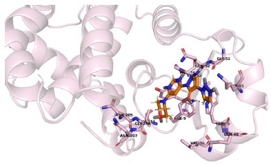
Author response image 2.

Molidustat docking with mutated GSTP1, Asn205 mutated to Gln205

Author response image 3.

Molidustat docking with mutated GSTP1, Tyr39 mutated to Phe39

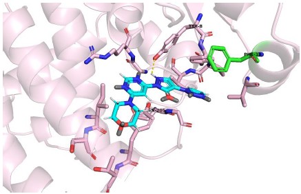
Author response image 4.

Molidustat docking with mutated GSTP1, Asn205 mutated to Ser205 and Tyr8 mutated to Phe8

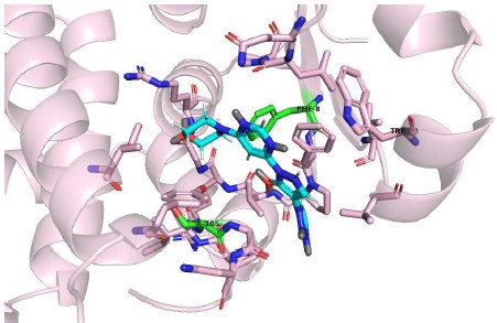
(3) Figure 5B and 5C: The metabolic imbalance phenotype observed upon dual knockout of PHD2 and GSTP1 requires rescue experiments to confirm on-target specificity.

We thank the reviewer for this important point and agree that rescue experiments could represent the most direct demonstration of on-target specificity for the metabolic phenotype observed in Figures 5B and 5C. These rescue experiments are necessary when working with single clones, as they allow for comparing a knock-out clone with a reconstituted pool and sidestep the issue of clonal heterogeneity.

In our case, we think that there is no advantage to doing so, as we work with pooled knockouts, so any clonal heterogeneity is diluted in the pool.

One could even make the case that such a rescue experiment would introduce additional artefacts. Combined loss of PHD2 and GSTP1 leads to reduced cellular viability, with decreased proliferation and increased apoptosis, consistent with a synthetic lethal interaction. To devise a rescue experiment, we would have to isolate a single-cell clone (the pool is not a complete 100% knock out, WT cells would outgrow the knock out cells). The isolation of such a clone that has overcome the anti-proliferative insult of the double knockout is likely to have a phenotype distinct from the original, pooled population, as would the rescued have from the WT cells. For these reasons, we have not performed rescue experiments in the current study. We have added the absence of a rescue as a limitation to the study in the discussion

“While genetic rescue experiments would provide definitive confirmation of on-target specificity, the pronounced loss-of-fitness and apoptotic phenotype observed upon combined PHD2 and GSTP1 loss limited the feasibility of establishing stable rescued double-knockout populations, and therefore represents a limitation of the current study.”

Reviewer #2 (Public review):

Summary:

The authors aimed to determine Molidustat targets and the potential utility of these findings. They clearly demonstrate that Molidustat interferes with GSTP1 and some other proteins on top of PHD2. They also demonstrate that PHD2 deletion is not sufficient to recapitulate Molidustat effects in cells and proteomes. Finally, they demonstrate synthetic lethality in organoids for Molidustat and APC deletion.

Strengths:

The data on Molidustat proteomes, GSTP1 binding, inhibition and metabolic health of organoids is really clear. All biochemical, docking and omic data are really strong. The potential impact of these findings could be the use of Molidustat in APC null tumours and awareness of potential off-target effects.

Weaknesses:

A main but minor weakness is that Molidustat also inhibits other PHDs, although these are less expressed. PHD1 has been shown to control the cell cycle and be expressed in the colon, where it is needed for viability. Although this does not explain the lack of effect of other PHD inhibitors, it does warrant some discussion. The use of MTT is not very good to detect viability when it measures metabolism; this also needs to be discussed and perhaps supplemented with colony or cell number measurements.

Great point, for this reason, we have assayed apoptosis throughout. In addition, we have added a clonogenicity assay with APC organoids. Organoid cells were treated with an acute dose of Molidustat. We subsequently measured the level of Lgr5 (a stem cell marker) and of the ability of the cells to generate organoids (these data have been added as Figure 5 F-G.)

Reviewer #3 (Public review):

In this paper, the authors revealed that Molidustat can induce a dose-dependent increase in Caspase-3/7 activity in the HT29 cell line, which is an APC-mutant colorectal cancer cell line. More importantly, they found that targeting PHD2 alone cannot cause cell death. By using thermal proteome profiling (TPP) and orthogonal chemical proteomic competition assays, they determined GTSP1 as a previously undiscovered off-target of Molidustat. They also revealed that combined PHD2 and GSTP1 loss leads to an increase in intracellular ROS and apoptosis. Moreover, they evaluated the effects of Molidustat in colonic organoids and showed that

Molidustat has a high selectivity for colonic organoids with activated WNT signaling and/or KRAS pathway alterations, and this effect is not reproduced by hydroxylase inhibition alone, providing a new potential approach to targeting both PHD2 and GTSP1 for the treatment of APC-mutant CRC.

Specific comments:

(1) What is the possible molecular mechanism of dual GSTP1/PHD2 loss, inducing cell death?

This is an important question. Our data support a model in which combined loss of GSTP1 and PHD2 disrupts cellular redox homeostasis, leading to accumulation of reactive oxygen species, increased GSSG/GSH ratios, and depletion of antioxidant buffering capacity. This redox imbalance is accompanied by downregulation of pro-survival pathways. In this context, activation of apoptotic signalling, as evidenced by increased caspase-3/7 activity and proteomic enrichment of apoptosis-associated pathways, contributes to the observed cell death phenotype.

While apoptosis is supported by our data, the magnitude of oxidative stress suggests that additional oxidative stress-associated cell death mechanisms may also contribute. We have clarified this point in the Discussion (Page 11).

(2) Can the authors mutate the binding site of Molidustat on GTSP1 to verify the in silico docking results?

This is a very important question. Currently, the model is of limited value. Reviewer 1 had a similar question. Can we refer you to Reviewer 1, question 2.

(3) Evidence for Molidustat inhibiting PHD2 activity or stabilising HIF-1α should be provided.

We thank the reviewer for this suggestion. Data showing HIF-1α stabilisation and evidence of downstream signalling is now added to Supplementary Figure 1.

Recommendations for the authors:

Reviewer #2 (Recommendations for the authors):

I only have minor suggestions:

Molidustat also inhibits other PHDs, although these are less expressed. PHD1 has been shown to control the cell cycle and be expressed in the colon, where it is needed for viability. Although this does not explain the lack of effect of other PHD inhibitors, it does warrant some discussion. The use of MTT is not very good to detect viability when it measures metabolism; this also needs to be discussed and perhaps supplemented with colony or cell number measurements.

This is correct, PHD1 is of particular interest, given the effects inhibition/knock-out has on the inflamed colon. We have added a new paragraph to the Discussion (Page 13) that addresses the isoform selectivity of Molidustat. We note that, although developed as a PHD2 inhibitor, Molidustat retains appreciable activity against PHD1 and PHD3 [4], and we discuss the non-redundant and in some contexts opposing roles of PHD1 and PHD2 in the colon, PHD1 loss is protective in DSS colitis [5] and restrains colitis-associated tumour growth, whereas PHD2 loss in the tumour and stroma is reported to inhibit metastasis and treatment response [6]. We further note that this pattern of isoform engagement is shared with other pan-PHD inhibitors that did not phenocopy Molidustat in our screens, indicating that PHD isoform profile alone is insufficient to explain Molidustat’s distinctive activity and pointing to GSTP1 off-target engagement as the key distinguishing feature. We argue that localised colonic delivery (as discussed earlier in the Discussion) would concentrate drug at the APC-mutant epithelium while limiting systemic exposure.

We fully agree with the reviewer, MTT measures metabolic activity/NADH levels rather than viability in the strict sense, and that this is particularly relevant for a compound that perturbs redox metabolism. We have added a clonogenicity assay in APC organoids (Fig. 5 F-G) to supplement the MTT and Cleaved Caspase 3 assays already present in the manuscript.

(1) Lee, J. K. et al. Directed evolution of CRISPR-Cas9 to increase its specificity. Nat. Commun. 9, (2018).

(2) Sakovina, L., Vokhtantsev, I., Vorobyeva, M., Vorobyev, P. & Novopashina, D. Improving Stability and Specificity of CRISPR/Cas9 System by Selective Modification of Guide RNAs with 2′-fluoro and Locked Nucleic Acid Nucleotides. Int. J. Mol. Sci. 23, (2022).

(3) Makar, A. N., Holkham, J., Lilla, S., Wilkinson, S. & von Kriegsheim, A. Overcoming preservation challenges to enable single-cell proteomics of fixed cell and tissue samples with retained proteome integrity. Preprint at https://doi.org/10.1101/2025.03.10.642380 (2025).

(4) Flamme, I. et al. Mimicking hypoxia to treat anemia: HIF-stabilizer BAY 85-3934 (molidustat) stimulates erythropoietin production without hypertensive effects. PLoS One 9, (2014).

(5) Tambuwala, M. M. et al. Loss of prolyl hydroxylase-1 protects against colitis through reduced epithelial cell apoptosis and increased barrier function. Gastroenterology 139, (2010).

(6) Leite de Oliveira, R. et al. Gene-Targeting of Phd2 Improves Tumor Response to Chemotherapy and Prevents Side-Toxicity. Cancer Cell 22, (2012).

eLife Assessment

This study used pupillometry to provide an objective assessment of a form of synesthesia in which people see additional color when reading numbers. It provides convincing evidence that subjective color ratings are matched by changes in pupil size that recapitulate brightness-mediated changes when exposed to the real color. The work provides a valuable contribution to the literature on both synesthetic perception and the use of pupillometry to probe perception and related psychological processes.

Reviewer #1 (Public review):

Summary:

Knowing that small pupil-size variations accompany brightness variations (even when these are illusory), the authors asked whether pupil constrictions would accompany the synesthetic perception of a brighter color (compared with a darker one), induced by the presentation of a black-white character. This grapheme-colour synesthesia is only experienced by few participants, sixteen of whom were enrolled in this study. The results reliably showed that a relative pupil constriction would "betray" the perception of a brighter color in these participants, while no such effect would be observed in control participants who were asked to report a color in association with each grapheme, even though they did not perceive any.

Strengths:

The main strength of the study lays in its combination of psychophysics (brightness ratings) and pupillometry, which allowed for showing clear-cut results.

Weaknesses:

I only see the following relatively minor weaknesses, namely:

- The pupil traces in Figure3 (main results) are heavily pre-processed (per-participant demeaned), loosing any feature besides the effect of interest. As I argued in my first review, I worry that this format gives unrealistic expectations about the effect (the perception of dark/bright colors do not generate a net dilation/constriction of the pupil; perception-related modulations of pupil size are always relative and generally small compared to the numerous other effects registered in pupil size; these include a pupil dilation that is more prominent in the controls and that gets analyzed later on in the manuscript; I do not think that eliminating one of the effects of interests from a main results figure helps the reader understand the results). In the revised manuscript, the authors addressed this concern by adding a Supplementary Figure 4, where a more complete representation of the results is shown (traces from individual trials are baseline corrected and averaged, resulting in more informative timecourses). I would strongly recommend that Supplementary Figure4 is brought to the main text (Figure3 could be presented in Supplementary).

- Responses to physical brightness modulations were only measured in the synesthethes group, not in controls. The authors point out that pupillary light responses have been thoroughly characterized in previous studies, and conclude that synesthethes' responses were in line with the expectations both in terms of amplitude and latency. However, as we are not dealing with standardized measurements, subtle differences in pupil reactivity across the two populations remain a possibility. I recommend that this possibility is mentioned in the discussion.

Impact:

This work is likely to improve our understanding of synesthesia, providing a new tool to quantify the subjective sensations; an interesting potential extension would be using pupillometry for tracking changes over time of the synesthetic experiences, opening up the possibility to evaluate the importance of learning for this peculiar experience.

Reviewer #2 (Public review):

Synesthesia is a neurological condition where stimulation of one sensory channel leads to involuntary, automatic, and consistent experience of another, unrelated percept. For example, Sir Francis Galton (1880, Nature) famously described the robust tendency of some individual (synesthetes) to associate numerals with a distinct color. Ever since, synesthesia keeps attracting a broad interest in the cognitive neurosciences in light of its implications for the study of domains such as perception, consciousness, and brain connectivity, among others.

Strauch, Leenaars, and Rouw measured pupil size in a group of 16 grapheme-color synesthetes and two matched control groups. The participants were presented with gray digits - that is, visual stimuli having identical physical properties in terms of brightness. Each participant subsequently rated the corresponding evoked color and brightness: unlike controls, synesthetes did so in a very consistent and reliable fashion. Accordingly, this was also shown in their pupils: despite the same objective luminance, digits associated with brighter percepts caused their pupils to constrict and digits associated with darker percepts caused their pupils to dilate more than controls. These results highlight how crossmodal correspondences are deeply rooted in synesthetes, and puts forward pupillometry as a particularly appealing biomarker for some phenomenological experience (at least those grounded in "brightness").

Further strengths of the technique are its temporal resolution and its responsiveness to several constructs. Across several tasks, the authors show for example that responses to synesthetic light are somewhat slower than responses to real light (i.e., they are likely mediated), but at the same time faster than responses to mental imagery. The role of mental imagery can also be reasonably dismissed when considering the second feature of pupil size: its responsiveness to mental effort and cognitive load. The pupils tend to dilate with demanding, challenging tasks, and this was the case when control participants were asked to report the color of a digit for which they did not consistently experience a synesthetic association. The same task was, instead, seemingly effortless for synesthetes, again speaking in favor of the automaticity of number-color correspondences in their case.

Overall, the findings by Strauch, Leenaars, and Rouw are highly significant for the field and likely to be impactful. The strength of their evidence, when accounting for the relatively small sample size and the inherent variability of both phenomenology (color perception and subjective reporting) and physiology (pupil size), is adequate and sufficiently convincing.

Comments on revisions:

I thank the authors for addressing all my comments in a satisfactory way. I think that the paper has improved, especially in terms of transparency of the reporting and clarity of the results.

Reviewer #3 (Public review):

Summary:

In the present study, the authors examined pupillary responses to uncolored stimuli (number graphemes) among number-color synesthetes and non-synesthetes. After seeing a digit, the synesthetes and active control participants were asked to indicate which color they perceived using three dimensions of hue, saturation, and lightness. The lightness values were the primary independent variable for follow-up analyses. To see how the pupil responded to psychologically "bright" and "dark" digits, the authors split the reported lightness values at the median and plotted them. The synesthetes showed a pupillary constriction to digits they perceived as bright and dilation to digits they perceived as dark. Active control participants did not show that effect. In a subsequent block, only the synesthetes were shown the colors they reported perceiving as colored discs. Their pupillary responses were similar. The authors also found that the differences in pupillary responses between light and dark perceptions (with digits) were only slightly delayed in their onset to the perception of a colored disc, and therefore the color perception accompanying a digit is unlikely to be effortful or a retrieved association, but occurs rather automatically.

Strengths:

The authors employed a well-controlled and designed quasi-experiment comparing color-grapheme synesthetes to non-synesthetes and showed convincingly that the color perceptions accompanying graphemes alter the physical perception of brightness. They also made a reasoned attempt to ruled out the possibility that color associations are occurring effortful via retrieved associations.

The follow are questions which I had asked in a first round of reviews, and which were answered adequately by the authors:

(1) Are the pupillary responses among synesthetes, which objectively do not seem to match the degree of physical stimulation entering the retina, in any way maladaptive for eye functioning? I understand the constriction/dilation of the pupil to not only benefit visual acuity but also to protect the retina from damage. Are synesthetes at any risk of retinal damage due to over-dilation of the pupil to brighter stimuli? Or are these effects of a magnitude that is too small to matter? As reported in arbitrary units, it was hard to know how large these effects were in terms of measurable changes in dilation (e.g., millimeters).

(2) Likewise, is the automatic synesthetic merging of two percepts something that could be learned such that natural synesthetes and "artificial" synesthetes would look similar? For example, if a group of non-synesthetic participants were to learn a color-grapheme association to automaticity, would you expect their pupillary responses to the graphemes look similar to the synesthetes? If so (or if not), what would this tell us anything about the phenomenology of synesthesia?

(3) Do the synesthetic perceptions of digit graphemes merge in a sensible way? For example, if a synesthete sees a particular color with the digit 1, and a different color with the digit 9, what do they perceive when they see 19? or 1-9, or 1 9? Is there color blending, or an altogether different color perception?

Author response:

The following is the authors’ response to the original reviews.

eLife Assessment

This study used pupillometry to provide an objective assessment of a form of synesthesia in which people see additional color when reading numbers. It provides convincing evidence that subjective color ratings are matched by changes in pupil size that recapitulate brightnessmediated changes when exposed to the real color. The work provides a valuable contribution to the literature on both synesthetic perception and the use of pupillometry to probe perception and related psychological processes.

We were pleased to learn that our manuscript was of interest to the reviewers and the editor. We thank the reviewers for their useful feedback and have addressed all their comments in the revised version. We here give the most prominent changes as quotes.

We thank all reviewers and for their very helpful input.

Public Reviews:

Reviewer #1 (Public review):

Summary:

Knowing that small pupil-size variations accompany brightness variations (even when these are illusory), the authors asked whether pupil constrictions would accompany the synesthetic perception of a brighter color (compared with a darker one), induced by the presentation of a blackwhite character. This grapheme-colour synesthesia is only experienced by a few participants, sixteen of whom were enrolled in this study. The results reliably showed that a relative pupil constriction would "betray" the perception of a brighter color in these participants, while no such effect would be observed in control participants who were asked to report a color in association with each grapheme, even though they did not perceive any.

Strengths:

The main strength of the study lies in its combination of psychophysics (brightness ratings) and pupillometry, which allowed for showing clear-cut results.

Weaknesses:

Some relatively minor weaknesses concern the ancillary analyses, which tackle secondary questions and are not entirely convincing.

(1) The linear mixed model approach is a powerful way to identify important variables, but it does not clarify whether the key factors are between-subject or between-trial variations. Some variables are inherently defined at a subject level (e.g., PA scores), others are not. I would strongly recommend an alternative visualisation of the results to examine inter-individual variability.

Visualizing the highly idiosyncratic effects is indeed challenging. Addressing R1’s point 4 and a point brought up by R2, we updated all figures to now visualize pupil size in millimeters instead of arbitrary units. Furthermore, we added a supplementary figure (supplementary figure 4) that visualizes pupil size change without demeaning (please see reply to point 4).

To get a better grasp of the interaction between lightness and coupling strength, we further included the supplementary figure 5 that splits by lightness and coupling strength in synesthetes.

Furthermore, as this review and response will be publicly available, Author response image 1 provides participant-mean traces per lightness bin in addition to the overall means and hopefully makes the stability/variability of effects visually clearer (in addition to the strip plots that attempt this for the average response).

Author response image 1.

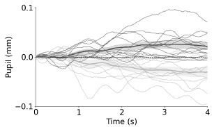
We hope that these additional visualizations make the effects of interest more transparent. Ultimately, however, the LME figure likely provides the information best, albeit at the cost of complexity.

(2) It is not clear why taking the first derivative of pupil size in Figure 5 would isolate the effect of arousal, eliminating those of luminance and contrast changes (in fact, one could argue for the opposite, since arousal effects are generally constant for extended periods of time while contrast effects are typically more local and transient).

First, please note that the results in 2.3.1 cannot be explained by task or context effects such as luminance and contrast: the exact same active color reporting task (same task and context) was presented to synesthetes and non-synesthetes.

Indeed, the reviewer is correct that the first derivative does not eliminate other concurrent pupil-driving effects, that was expressed wrongly in our original text. Indeed, any stimulus-locked effect, such as the luminance and contrast effects, but also the effort effect will reflect similarly in the derivative measure.

We did take the derivative because pupil responses driven by other non-trial related activity, such as increasing tiredness or excitement over the course of trials differ almost by necessity between participants, thus creating variability. However, these effects are most likely happening at a slower timescale and thus show less in the derivative measure. Accordingly in past research, we previously found clearer response-locked effects in the past when using a derivative measure (Douze et al., 2025; Ten Brink et al., 2024). This way, we also hoped to get rid of such variability that happens between participants for this between participant analysis.

Even if we were to use the same baseline corrected analysis, we would arrive at the same conclusion: we here directly compared baseline-corrected pupil sizes by taking individual differences into account (using a LME). In other words, we tested for the same question, but not relying on the derivative. We thus compared baseline-corrected pupil sizes using over-time LMEs. Group (active control vs. synesthete) gained significance between ~1.7s and 3s, aligning with the derivative-based result.

Author response image 2.

t-values of a per-time point LME predicting pupil response from group (synesthete/active control) Group reached significance.

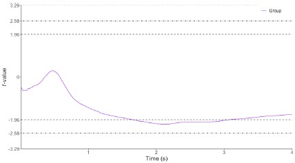
In sum, we deem the derivative more powerful/more appropriate in this context, but the interpretation of findings does not hinge on that analysis choice (as can be seen in the Author response image 2).

We corrected the claims on the derivative as a measure cleaning out other effects that indeed was oversimplified as it stood. We now write:

“Mental effort presents in task-evoked pupil dilations, yet other factors simultaneously affect the pupil, such as luminance and contrast changes at trial onset, as well as slower trends across the session (e.g., fatigue). To reduce the influence of these slower, non-trial-locked fluctuations while retaining the trial-evoked dynamics, we calculated the first derivative of the pupil time course to assess the velocity of pupillary changes (Butterworth filter, 18 Hz, order 3, 2.5 Hz lowpass, following our previous works [60, 61]).”

Douze, B. T., Ten Brink, A. F., Dijkerman, H. C., & Strauch, C. (2025). Pupil responses objectively index pharmacologically altered tactile sensitivity. Cortex, 193, 90-104.

Ten Brink, A. F., Heiner, I., Dijkerman, H. C., & Strauch, C. (2024). Pupil dilation reveals the intensity of touch. Psychophysiology, 61(6), e14538.

(3) It is a pity that responses to physical brightness modulations were only measured in the synesthete group, not in controls, as this would have allowed for ruling out differences in pupil reactivity across the two populations.

The reviewer is correct that this would allow additional comparisons, but argue that light responses in healthy control samples are very well documented and stereotypical. For instance, Bergamin & Kardon (2003) provide very systematic latency estimations, for low-luminance change stimuli in the realm of about 320ms that can accelerate to about 250ms for very strong luminance changes. Our relatively small luminance increments should thus be expected in this range. Indeed, this also well describes the response latencies we observed in synesthetes when exposed to the colored disks. While there is no detailed information about participants in Bergamin & Kardon (2003), data from previous studies shows very similar pupil light response profiles in a healthy student control population that matches our synesthetes well demographically (Strauch, Romein et al., 2022 Figure 2a, exact same lab as for the present study; Koevoet et al., 2025 Figure 3a). See also the further responses, baseline pupil size in millimeters across groups did not differ.

Together, we can safely conclude that pupil light responses in synesthetes are not different from pupil light responses in controls. We agree with the reviewer that this is a sensible point to also make in the manuscript:

“Specifically, pupil size first responded significantly to physical luminance after 330 ms (see Supplementary Figure 7 for per-timepoint LME; in line with response latencies of similar control populations, see Bergamin & Kardon [52], Koevoet et al. [40], and Strauch et al. [53]), but only responded significantly to synesthetic lightness at about 870 ms (see also Figure 3c vs e and Figure 4 for per-timepoint LME)”.

Bergamin, O., & Kardon, R. H. (2003). Latency of the pupil light reflex: sample rate, stimulus intensity, and variation in normal subjects. Investigative Ophthalmology & Visual Science, 44(4), 1546-1554.

Koevoet, D., Naber, M., Strauch, C. & Van der Stigchel, S. Presaccadic Attention Shifts Up-and Downwards: Evidence From the Pupil Light Response. Psychophysiology 62, e70047 (2025).

Strauch, C., Romein, C., Naber, M., Van der Stigchel, S., & Ten Brink, A. F. (2022). The orienting response drives pseudoneglect—Evidence from an objective pupillometric method. Cortex, 151, 259-271.

(4) Another concern is with the visualisation of the pupil traces in Figure 3 (main results); these were heavily pre-processed (per-participant demeaned), losing any feature besides the effect of interest and generating the unrealistic expectation that perception of dark/bright colors generate a net dilation/constriction of the pupil - whereas perception-related modulations of pupil size are always relative and generally small compared to the numerous other effects registered in pupil size. It would be far better to see the actual profiles, preserving the unfolding of dilations and constrictions over time, especially since these are further analysed in Figures 4 and 5.

Indeed, the expectation that any dark synesthetic experience would lead to pupil dilation whereas any bright synesthetic experience would lead to constriction is not warranted – it would only do that relative to the counterfactual of not having that experience.

Many factors affect the pupillary signal at the same time, and often differently across individuals (think of tiredness etc.), making merely baseline corrected traces seemingly noisy. Our visualization highlights that there is a systematic part to that variation that lies in the synesthetic brightness experience.

Visualizing the effects of idiosyncratic experiences, varying within and between participants is challenging. For the theoretical insight brought about through our paper in Figure 4 (synesthesia being sensory in nature), demeaning is favorable in our opinion as it isolates the effect of interest in visualization. However, for methodological reasons and to better show effect sizes etc., there is certainly use in additional transparency. We now thus provide non-demeaned traces in the supplementary material as the reviewer suggested and also refer to these in the main manuscript. Furthermore, all figures are now provided in millimeters, with all pupil related analysis being rerun and updated to this end (without qualitative changes to the results). This should further rectify possibly inflated expectations about the absolute size of effects and allows to put effects into perspective across studies. We now added:

“Pupillary data were transformed from arbitrary eyelink units to millimeters using a conversion factor obtained with an artificial eye (see Hayes & Petrov, 2016).”

Hayes, T. R., & Petrov, A. A. (2016). Mapping and correcting the influence of gaze position on pupil size measurements. Behavior research methods, 48(2), 510-527.

Impact:

Despite these weaknesses, and especially if they are adequately addressed in the review, this work is likely to improve our understanding of synesthesia, providing a new tool to quantify the subjective sensations; an interesting potential extension would be using pupillometry for tracking changes over time of the synesthetic experiences, opening up the possibility to evaluate the importance of learning for this peculiar experience.

We were happy to read our manuscript was evaluated this positively and hope that our replies can address the remaining smaller concerns and make findings more transparent to the readers.

Reviewer #2 (Public review):

Synesthesia is a neurological condition where stimulation of one sensory channel leads to involuntary, automatic, and consistent experience of another, unrelated percept. For example, Sir Francis Galton (1880, Nature) famously described the robust tendency of some individuals (synesthetes) to associate numerals with a distinct color. Ever since, synesthesia has continued to attract a broad interest in the cognitive neurosciences in light of its implications for the study of domains such as perception, consciousness, and brain connectivity, among others.

Strauch, Leenaars, and Rouw measured pupil size in a group of 16 grapheme-color synesthetes and two matched control groups. The participants were presented with gray digits - that is, visual stimuli having identical physical properties in terms of brightness. Each participant subsequently rated the corresponding evoked color and brightness: unlike controls, synesthetes did so in a very consistent and reliable fashion. Accordingly, this was also shown in their pupils: despite the same objective luminance, digits associated with brighter percepts caused their pupils to constrict, and digits associated with darker percepts caused their pupils to dilate more than controls. These results highlight how crossmodal correspondences are deeply rooted in synesthetes, and put forward pupillometry as a particularly appealing biomarker for some phenomenological experience (at least those grounded in "brightness").

Further strengths of the technique are its temporal resolution and its responsiveness to several constructs. Across several tasks, the authors show, for example, that responses to synesthetic light are somewhat slower than responses to real light (i.e., they are likely mediated), but at the same time faster than responses to mental imagery. The role of mental imagery can also be reasonably dismissed when considering the second feature of pupil size: its responsiveness to mental effort and cognitive load. The pupils tend to dilate with demanding, challenging tasks, and this was the case when control participants were asked to report the color of a digit for which they did not consistently experience a synesthetic association. The same task was, instead, seemingly effortless for synesthetes, again speaking in favor of the automaticity of number-color correspondences in their case.

Overall, the findings by Strauch, Leenaars, and Rouw are highly significant for the field and likely to be impactful. The strength of their evidence, when accounting for the relatively small sample size and the inherent variability of both phenomenology (color perception and subjective reporting) and physiology (pupil size), is adequate and sufficiently convincing.

We were glad to read this overall very positive assessment of our work and thank the reviewer for the additional non-public suggestions for improvements.

Reviewer #3 (Public review):

Summary:

In the present study, the authors examined pupillary responses to uncolored stimuli (number graphemes) among number-color synesthetes and non-synesthetes. After seeing a digit, the synesthetes and active control participants were asked to indicate which color they perceived using three dimensions of hue, saturation, and lightness. The lightness values were the primary independent variable for follow-up analyses. To see how the pupil responded to psychologically "bright" and "dark" digits, the authors split the reported lightness values at the median and plotted them. The synesthetes showed a pupillary constriction to digits they perceived as bright and dilation to digits they perceived as dark. Active control participants did not show that effect. In a subsequent block, only the synesthetes were shown the colors they reported perceiving as colored discs. Their pupillary responses were similar. The authors also found that the differences in pupillary responses between light and dark perceptions (with digits) were only slightly delayed in their onset to the perception of a colored disc, and therefore, the color perception accompanying a digit is unlikely to be effortful or a retrieved association, but occurs rather automatically.

Strengths:

The authors employed a well-controlled and designed quasi-experiment comparing colorgrapheme synesthetes to non-synesthetes and showed convincingly that the color perceptions accompanying graphemes alter the physical perception of brightness. They also made a reasoned attempt to rule out the possibility that color associations are occurring effortfully via retrieved associations.

We appreciate the positive assessment and useful suggestions for revision.

Weaknesses:

There are some areas in which the implications of these findings could be elaborated upon. I had the following questions:

(1) Are the pupillary responses among synesthetes, which objectively do not seem to match the degree of physical stimulation entering the retina, in any way maladaptive for eye functioning? I understand the constriction/dilation of the pupil to not only benefit visual acuity but also to protect the retina from damage. Are synesthetes at any risk of retinal damage due to over-dilation of the pupil to brighter stimuli? Or are these effects of a magnitude that is too small to matter? As reported in arbitrary units, it was hard to know how large these effects were in terms of measurable changes in dilation (e.g., millimeters).

This is an interesting point. Some argue that pupil size changes in a mid-range mildly affect optics thus affecting detection performance, contrast perception, and depth of field (Eberhardt et al., 2022, Mathôt & Ivanov 2019, Ruuskanen, Boehler, & Mathôt, 2025), rather than serving a protective role for the retina (Mathôt, 2018). Indeed, any effects reported here were quite small. We agree with the reviewer that this can be made more accessible by reporting effects in millimeters. We thus now adjusted all figures accordingly and write in the methods section:

“Pupillary data were transformed from arbitrary eyelink units to millimeters using a conversion factor obtained with an artificial eye (see Hayes & Petrov, 2016).”

Note that even the largest effects here (those elicited by physical luminance change in block 2 for the synesthetes) only caused differences in pupil size of about 0.3mm. This lies below the maximal pupil dilations observable in response maximal effort (about 0.5mm), for instance, and substantially below the full range of pupil size changes elicited through strong luminance stimulation (several millimeters). We therefore deem the changes in pupil size as obtained in our study too minor to be practically maladaptive for optics/perception.

Eberhardt, L. V., Strauch, C., Hartmann, T. S., & Huckauf, A. (2022). Increasing pupil size is associated with improved detection performance in the periphery. Attention, perception, & psychophysics, 84(1), 138-149.

Hayes, T. R., & Petrov, A. A. (2016). Mapping and correcting the influence of gaze position on pupil size measurements. Behavior research methods, 48(2), 510-527.

Mathôt, S., & Ivanov, Y. (2019). The effect of pupil size and peripheral brightness on detection and discrimination performance. PeerJ, 7, e8220.

Mathôt, S. (2018). Pupillometry: Psychology, physiology, and function. Journal of cognition, 1(1), 16.

Ruuskanen, V., Boehler, C. N., & Mathôt, S. (2025). The Interplay of Spontaneous Pupil-Size Fluctuations and EEG Power in Near-Threshold Detection. Psychophysiology, 62(3), e70035.

(2) Likewise, is the automatic synesthetic merging of two percepts something that could be learned such that natural synesthetes and "artificial" synesthetes would look similar? For example, if a group of non-synesthetic participants were to learn a color-grapheme association to automaticity, would you expect their pupillary responses to the graphemes look similar to the synesthetes'? If so (or if not), what would this tell us anything about the phenomenology of synesthesia?

We find this question most interesting. Likely, different synesthesia researchers wouldn’t even fully agree on the most plausible answers to these questions. Training studies have shown that nonsynesthetes can be trained to associate particular colors to particular graphemes, as revealed in the synesthetic Stroop effect: interference effects of the learned color onto reporting the typeface color of the grapheme. The degree to which non-synesthetes can be trained to become similar to synesthetes is however still topic of debate.

We now discuss as follows:

“Future studies could examine to what degree training a non-synesthete to associate specific colors to particular inducers (e.g., digits), can provide similar patterns of results as genuine synesthesia (Bor et al., 2014, Colizoli et al., 2012, Rothen & Meier, 2014). Could learning produce similar brightness-related pupil effects in non-synesthetes? Similarly, would effort-linked responses diminish with increased training duration? The perhaps most interesting question relates to response latencies: Would a trained participant ever be able to produce brightnessrelated pupil effects as fast as a synesthete?”

Bor, D., Rothen, N., Schwartzman, D. J., Clayton, S., & Seth, A. K. (2014). Adults can be trained to acquire synesthetic experiences. Scientific reports, 4(1), 7089.

Colizoli, O., Murre, J. M., & Rouw, R. (2012). Pseudo-synesthesia through reading books with colored letters. PloS one, 7(6), e39799.

Rothen, N., & Meier, B. (2014). Acquiring synaesthesia: insights from training studies. Frontiers in human neuroscience, 8, 109.

(3) Do the synesthetic perceptions of digit graphemes merge in a sensible way? For example, if a synesthete sees a particular color with the digit 1, and a different color with the digit 9, what do they perceive when they see 19? or 1-9, or 1 9? Is there color blending, or an altogether different color perception?

This is a very interesting question indeed. While each synesthete will have their own specific expression of synesthesia, there are regularities in how a combination of digits evokes synesthetic color. First, if asked about the color of a specific digit, each digit keeps its own color, as the color of a digit is linked to the identity of the digit (Dixon et al., 2006). Context effects are however possible, in particular when context alters the interpretation of the digit (Myles et al., 2003). A particularly common context in a multi-digit number is a dominant first digit, spreading its color to the subsequent digits in the number. However, as the digit color is linked to digit identity, what does ‘not’ happen is a mixing of colors into a qualitatively new color; for example, a yellow "1" and blue "9" do not merge into a green "19".

Dixon, M. J., Smilek, D., Duffy, P. L., Zanna, M. P., & Merikle, P. M. (2006). The role of meaning in grapheme-colour synaesthesia. Cortex, 42(2), 243-252.

Myles, K. M., Dixon, M. J., Smilek, D., & Merikle, P. M. (2003). Seeing double: The role of meaning in alphanumeric-colour synaesthesia. Brain and Cognition, 53(2), 342-345.

Many thanks for the constructive assessment of our work.

Recommendations for the authors:

Reviewer #1 (Recommendations for the authors):

(1) I am not sure I'd use the term 'cross-modal' given that the case considered here (graphemecolor) is purely visual.

The reviewer is absolutely right: the term 'cross-modal' has a historical background rather than reflecting an exact factual accuracy. The term is still commonly used however, as it readily reflects how the induced additional experience is always of a different (sub)type than the inducing experience. There is a cross-over between experiences that might occur within the same sensory modality, or even induce awareness of a particular concept. But key to synesthesia is the crossover experience as the inducer and concurrent are different (sub)types of experiences. For example, seeing a letter can evoke a synesthetic experience of seeing a color, or evoke awareness of a particular gender or personality of that letter, but does not evoke another letter. To remain consistent with literature, we refer to 'cross-modality' when explaining the link to previous literature, but generally switched to using 'cross-over experience':

“Therefore, synesthesia might provide a unique window into how the brain’s constructive processes can generate additional, conscious content, in cross-over experiences, often across modalities, going all the way down to the level of sensory phenomenology.”

We adjusted throughout the manuscript accordingly.

(2) I would not recommend focusing the introduction on the problem of qualia; this is a much more general and complex question than the one addressed in the study; the space of the introduction may be better used to present the actual object of study, giving a better picture of the synesthetic phenomenon and of previous work aimed at characterising it (behavioural, including PA scores and consistency measures, and neuroimaging). It is important to discuss how the pupillometric approach differs from the previously adopted neuroimaging techniques and what it can add to those.

We agree that qualia is a very general and complex question. However, we respectfully disagree that this complex question is not the object of the study. What is remarkable about synesthesia is not the presence of an additional perceptual association per se, but the presence of a specific perceptual experience. As illustration, think of a test where an unconscious color association to the word 'banana' was tested. While a generic 'yellow' could semantically be linked and would likely be obtained in the (e.g. priming) experimental results, a follow-up question of picking on a color wheel the exact shade of yellow to this association, or describing the perceptual sensation of the color, would be non-sensical to the participants.

This sharply contrasts with the current study: synesthetes, but not non-synesthetes, indicate a perceptual sensation of additional colors, and subsequently indeed the sensory properties of this percept (experienced brightness) affects the objective reflection of this sensation (pupil size) in synesthetes but not in non-synesthetes. In our view, the presence of additional qualia is key in understanding what sets synesthetic apart from non-synesthete associations, including so-called cross-modal correspondences (unconscious consistent associations across modalities, common to us all). We even believe that the reported qualia is what makes synesthesia so interesting in the first place. We now more clearly explain this link to qualia better in the introduction.

"The most remarkable aspect of synesthesia is the subjective perceptual phenomenology of the induced colors, setting these sensations apart from color memory, thought, or amodal association. The contrast between synesthetes and non-synesthetes can thus offer an interesting doorway into examining qualia, the subjective perceptual phenomenology or first person (what's-it-like) perspective."

We also improved the explanation of the synesthetic phenomenon, including a more detailed characterisation of behavioural measures (including consistency scores) and added neuroimaging studies. These changes have been incorporated into the text in response to previous comments (point 1- reviewer 1).

Please note that we have chosen not to include more detailed discussion of PA scores. Our results show a trend but do not allow for a conclusive interpretation on PA scores, and we feel that placing greater emphasis on this topic might therefore be confusing or even misleading. Still, it would be a very interesting topic for follow-up research to examine how alterations in characteristics of the synesthetic experience influence pupil responses.

The different synesthesia types all share the defining characteristics of an additional conscious and consistent experience. Synesthetes can verbally report their additional experience, and synesthetic sensations can be measured in behavioral paradigms such as the ’synesthetic Stroop’ effect, or brain activation patterns in sensory cortex [15]. Furthermore, test-retest paradigms show how synesthetic, but not non-synesthetic associations are highly specific and consistent [16-18]. Thus, over the past decades, research has established synesthesia as a ’real’ condition that can reliably be identified using behavior, neurophysiology, and neuroimaging [11, 13, 15–21]. The most remarkable aspect of synesthesia is the subjective perceptual phenomenology of the induced additional sensation, i.e., color in grapheme-color synesthesia. This sets synesthetic sensations apart from (color) memory, thought, or amodal association. Synesthesia can thus offer an interesting doorway into examining qualia, the subjective perceptual phenomenology or first person (what’s-it-like) perspective.

We now discuss the pupillometric approach as it differs from the previously adopted neuroimaging techniques as follows:

“Compared to neuroimaging studies [12,15,51], pupillometry may offer a more direct window into synesthetic phenomenology, as the directionality between pupil light reflex and perceived brightness is straightforward. Finally, improved understanding of the underlying processes can be obtained by contrasting responses to perceived versus actual (physical) brightness, given that the pupil light reflex is a well-characterised reflex arc involving few inferential steps.

This adds to the explanation that was already present on how the current approach differs from previous techniques, and what it can add to those techniques:

"Instead, current paradigms capturing synesthesia employ objective measures, but fail to capture its phenomenology [16, 17, 21, 23]."

(3) There are a few typos and word repetitions.

Many thanks – we identified typos and repetitions after another set of careful reads and hope to have eradicated them completely now.

Reviewer #2 (Recommendations for the authors):

I am overall very supportive of this work, but addressing the following points may enrich it further:

(1) Paragraph 2.2.1. Here, models do not seem to compare synesthetes versus controls but rather assess the effects of interest separately in the two groups. The fact that experimental effects are significant in synesthetes, but not in controls, does not tell us much about differences between groups. Controls (e.g., Figure 3) do show a similar trend, albeit clearly smaller. There is one passage in which this issue appears to be tackled (page 10): "Critically, in an LME ran on synesthetes and controls and using only graphemes and the interaction of group and lightness as predictors, we found lightness to predict pupil size in synesthetes (t = -2.754, p = 0.006), but not controls (t = -1.134, p = 0.257)." But I am not sure that the reported statistics belong to the interaction - they seem to refer to the lightness effect within each group, not the difference.

This is an important point, power for between-group comparisons is inherently limited for n = 16 per group (while still feasible for overall responses, things become trickier when less trials remain). A simple model of pupil ~ grapheme + group * lightness_scaled + (1 | participant) shows no significant interaction (despite one group showing the effect and the other not showing the effect significantly). The additional negative effect for group is in line with the effort-related effect reported later in the manuscript. Where does this leave us? Based on the lightness responses alone, the group difference can be characterized as a quantitative distinction, but the degree in which it is also a qualitative distinction cannot clearly be determined from current data. We revised the manuscript to make sure that such an interaction is not implied/ point to the absence of the significance of that interaction.

The sensory nature of synesthetic color is supported by within-synesthete analyses, where coupling strength parametrically modulates the lightness-pupil relationship in a theoretically predicted manner. Importantly, the effort-related findings provide a complementary and statistically robust group comparison: synesthetes and controls performing the identical colorreporting task showed significantly different pupil dilation rates, directly demonstrating that the two groups differ in how they access color information. Together, these two independent pupillometric signatures, one tracking perceptual quality, one tracking effort, converge on the same conclusion and mutually reinforce the interpretation that synesthetic color constitutes genuine sensory phenomenology.

Author response image 3.

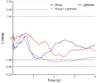
We now make this more explicit in the manuscript as follows:

“We found significant modulations of pupil size by the lightness of the grapheme's synesthetic color - sustained and in the to-be-expected time window. Specifically, the pupil constricted more for brighter reported colors, and dilated more for darker reported colors, as predicted (Average pupil size 800-4000ms, t = -3.601, p < 0.001). In an LME ran for synesthetes and controls and using only graphemes and lightness as predictors, we found lightness to predict pupil size in synesthetes (t = 2.844, p = 0.004), but not controls (t = 0.606, p = 0.544). However, when taking group as interacting factor in a joint LME, there was no interaction of lightness and group (t = -0.949 p = 0.342).”

and

“For controls a separate model was run, now without the PA score as predictor (not assessed for controls). Neither lightness (t = -0.815, p = 0.415), coupling strength (t = 0.438, p = 0.661), nor their interaction gained significance (t = -1.058, p = 0.290; all for average pupil size between 800 ms and 4000 ms). Critically, we also ran a LME with the three-way interaction of coupling strength, group, and lightness (Wilkinson notation: pupil = grapheme + group + lightness * group + coupling strength * lightness * group + (1 | participant)). This analysis revealed a significant three-way interaction between lightness, coupling strength, and group (F = 3.86, p = .021), indicating that the lightness × coupling strength effect on pupil size was not equivalent across groups. Decomposing this interaction by group, the lightness × coupling strength slope was significant in synesthetes (t = 2.59, p = .010) but not in controls (t=-1.01, p=.311), suggesting that reported lightness and its coupling strength were more consistently related to pupil size in synesthetes than in controls. Note however, that this decomposition does not directly test whether the two slopes significantly differ from each other, however. Lastly, pupil size was marginally larger in controls than in synesthetes (t = 1.94, p = .062; see later sections for more in-depth analyses)”

(2) The authors choose to analyze pupil size in arbitrary eye tracker units. This is fine, although I would recommend assessing and reporting whether the average pupil size (e.g., during the baseline) is roughly comparable between groups. The size of the effects may be difficult to compare between groups in the presence of very different baseline pupil size.

Please see Author response image 4 for Baseline pupil sizes per group in millimeters. There were no differences between groups.

Author response image 4.

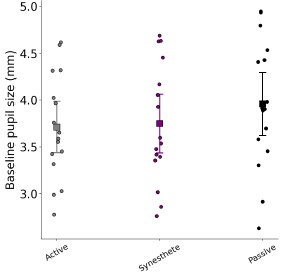
F2, 45) = 0.707, p = 0.499 (One-way Anova).

We now write:

“Baseline pupil sizes did not differ between groups (F(2, 45) = 0.707, p = 0.499).”

We agree with the reviewer that millimeters are a more intuitive measure and updated all figures throughout manuscript and supplementary materials accordingly. We also briefly added to signal processing that this conversion was applied.

“Pupillary data were transformed from arbitrary eyelink units to millimeters using a conversion factor obtained with an artificial eye (see Hayes & Petrov, 2016).”

Hayes, T. R., & Petrov, A. A. (2016). Mapping and correcting the influence of gaze position on pupil size measurements. Behavior research methods, 48(2), 510-527.

(3) If I understand correctly, the main task counted 120 trials overall (12 per digit). It seems, however, that only 3 and 4 participants remained with at least 50 trials (or 25 per median split by lightness) after preprocessing. This appears to be quite a massive data loss: is there a reason behind it? Please also clarify: the overall percentage of discarded trials; whether the median split by lightness was computed on all responses or only on those of the remaining, valid trials.

This is an important point for clarification indeed. The exclusion of participants in Figure 3 applies only to that particular visualization, not to the statistical analyses. The linear mixed effects models (LMEs) used all available valid trials from all participants, with no participant-level exclusions. The figure-specific threshold (≥25 trials per median-split bin) was applied purely for display clarity, as plotting participants with very few trials per bin would produce unreliable/noisy and thus visually misleading traces (as we note in the figure caption and point readers to Supplementary Figure 1, which shows the same visualization without any exclusions).

Since the paradigm required participants to repeat discarded trials until 120 valid trials were collected, all participants thus contributed exactly 120 valid trials to the analyses. There was therefore no data loss at the analysis level for the LME that is central to the claims of the manuscript (albeit more complex to grasp than the t-tests between bins).

Why were there sometimes so little trials per brightness bin?

First, participants differed in how dark or bright (synesthetic or forced-report) colors were overall, meaning that differing proportions thereof would fall above or below the 0.5 cutoff that overall, well represented the sample (but not necessarily every single participant). Note that this median split was not performed per individual but across all color reports to allow an apples-to-apples comparison.

Second, participants often reported colors that differed in Hue and Saturation, but not Lightness. This is in line with synesthetes picking certain colors more often than others, as compared with non-synesthetes (Rouw & Root, 2019; Ward et al., 2025).

We now include a new Supplementary Figure that visualizes responses on the Hue and Saturation dimensions of HSL space for both synesthetes and controls; fully saturated reports appear on the outer edge. We refer to the supplementary figure in the caption of Figure 2 as follows:

"See Supplementary Figure 1 for color reports on the hue and saturation axes.”

Rouw, R., & Root, N. B. (2019). Distinct colours in the ‘synaesthetic colour palette’. Philosophical Transactions of the Royal Society B: Biological Sciences, 374(1787).

Ward, J., Maciel, S., Rouw, R., Simner, J., & Root, N. (2025). Synaesthesia is linked to differences in music preference and musical sophistication and a distinctive pattern of sound-color associations. Psychology of Music, 53(3), 453-473.

Minor points:

(1) "Building on this evidence, we hypothesized that the cross modal color phenomenology in synesthesia can, if truly sensory in nature, could likewise be (...)" -> may need rephrasing (can/could).

Many thanks, fixed.

(2) Caption of Figure 1: "Block 2 (synesthetes only): a colored disk and gray central patch, matching the average indicated color per digit, and the number and luminance of pixels of said digit were presented to assess externally triggered light responses." -> I find this sentence a bit hard to follow; perhaps consider rephrasing it.

Agreed, we rephrased to:

Block 2 (synesthetes only): a colored disk was presented, colored according to the synesthete's average indicated color for that digit. At its center sat a gray patch matching the luminance and pixel area of the original digit from Block 1, together allowing assessment of externally triggered light responses.

(3) Figure 2 b: Consider truncating the y-axis to 1 if that improves the visualization.

We adjusted the axis accordingly and added a bit more detail in the caption for the interpretation of the measure.

(4) Caption of Figure 3 points to "see Supplementary Figure 1", but it should probably be SF2.

Many thanks for spotting, all references to supplementary figures have been checked and are corrected now.

Elvio Blini

Reviewer #3 (Recommendations for the authors):

(1) As a minor comment, there are some terms that felt overused in the manuscript. For example, the words "extraordinary" and "exceptional" were used multiple times throughout. I believe I understand the authors to mean them in their descriptive sense (i.e., outside the realm of typical experience), but in context, those words make it seem like they are touting their own experiment as "exceptional" or "extraordinary," which I don't believe was their intention.

We agree. We removed words such as exceptional and extraordinary when they do not directly refer to the sensation throughout the manuscript (which is indeed how we intended to use it). We hope that this removes unnecessary and convoluting hyperbole.

(2) It seemed counterintuitive to me that the color consistency score would be reverse-coded. In this case, the scores actually seem to indicate inconsistency, rather than consistency. Perhaps the raw scores can be inverted for a more intuitive interpretation that aligns with the terminology. I understand that they were following a previous publication in their method (Rothen et al., 2013).

This manner of coding is counter-intuitive indeed. However, there are both logical and practical reasons to this approach. Importantly, this is indeed the standard way of reporting color consistency in synesthesia research (Carmichael et al., 2015; Eagleman et al., 2007; Root et al., 2025; Rothen et al., 2013). The calculation is based on a simple logic; a higher number reflects a larger distance in color space. An additional advantage is the clear and intuitive zero- reference: a score of zero implies choosing the exact same color. Finally, it intuitively reflects the distinction between synesthetes and non-synesthetes; there is by definition little variation across synesthetes (visualized at the bottom of the graph), then a 'cut-off line' (if consistency is used as diagnostic tool), and then the height of the range shows how large the range in consistency is, in that particular sample of non-synesthetes. In a way we therefore inherit a confusing definition/standard, but changing it would lead to new confusion instead. We now specifically clarify this in the caption as follows:

“Note that higher consistency is reflected in lower color distance, hence lower values [17].”

Carmichael, D.A., Down, M.P., Shillcock, R.C., Eagleman, D.M., Simner, J., 2015. Validating a standardised test battery for synesthesia: does the synesthesia battery reliably detect synesthesia? Conscious. Cogn. 33, 375–385

Eagleman, D.M., Kagan, A.D., Nelson, S.S., Sagaram, D., Sarma, A.K., 2007. A standardized test battery for the study of synesthesia. J. Neurosci. Methods 159 (1), 139–145.

Root, N., Chkhaidze, A., Melero, H., Sidoro -Dorso, A., Volberg, G., Zhang, Y., & Rouw, R. (2025). How “diagnostic” criteria interact to shape synesthetic behavior: The role of self-report and test–retest consistency in synesthesia research. Consciousness and Cognition, 129, 103819.

Rothen, N., Seth, A.K., Witzel, C., Ward, J., 2013. Diagnosing synaesthesia with online colour pickers: maximising sensitivity and specificity. J. Neurosci. Methods 215 (1), 156–160.

eLife Assessment

This study presents a large, systematically curated catalog of non-canonical open reading frames (ncORFs) in human and mouse through the reanalysis of nearly 400 Ribo-seq datasets using a standardized pipeline; the resulting atlas consolidates ncORF annotations across tissues and provides a valuable resource for investigating non-canonical translation and ORF emergence. The main conclusions are supported by consistent data processing and multiple computational measures of translation and conservation. While the pipeline is transparent and technically robust, some analytical criteria and dataset limitations could be described more explicitly, and several downstream conclusions would benefit from more cautious interpretation, some evolutionary inferences are primarily correlative; dataset heterogeneity, uneven tissue representation, and limited experimental validation also constrain the strength of a subset of the findings. Overall, the evidence is solid, and the resource is likely to be broadly beneficial to the community.

Reviewer #1 (Public review):

This work compiles a comprehensive atlas of ncORFs across mammalian tissues and cell types, derived from reanalysis of ~400 public ribosome profiling datasets. The authors then evaluate cross-species conservation and functional signatures, proposing that evolutionarily ancient ncORFs tend to have higher translation potential, stronger expression, and closer relationships with canonical coding sequences.

Strengths:

In general, the study provides a large-scale and timely resource of annotated ncORFs, which could be broadly useful for the community. The authors collected ~400 public ribosome profiling datasets for annotations of ncORFs, which, to my best knowledge, is the largest collection of data for such purpose. The catalog could facilitate future investigations into ncORF biology and broaden understanding of the coding potential of the "non-coding" genome.

Weaknesses:

Based on the ncORF catalog, some of the analyses were not properly done. Some of the results are descriptive.

(1) Bias and representations of data source. Public ribo-seq datasets are unevenly distributed across tissues and cell lines, raising concerns about heterogeneity and underrepresentation of certain contexts. This may limit the generalizability of the catalog.

(2) The discussion on modular domains of ncORFs is unclear, and the claim that they may originate via TE-related mechanisms is not well supported. Stronger evidence or clearer reasoning is needed.

(3) The conservation comparisons are not fully convincing. Figure S7 shows only mild differences between ncORFs and CDS, and statistical significance is not clearly demonstrated. Comparisons with other non-coding RNAs should be added, and overlapping sequences between ncORFs and CDS should be excluded to avoid bias.

(4) Figure 3 indicates that some ncORFs are subject to evolutionary constraints. This is not surprising. The authors should provide further analyses on more detailed features of these "conserved" ncORFs vs. the "non-conserved" ones. Some pretty informative works have been done in drosophila, worms, mouse, and human. Figure 3 suggests some ncORFs are under evolutionary constraint, but this is not unexpected. More granular analyses contrasting "conserved" versus "non-conserved" ncORFs would be informative. In fact, small ORFs, especially uORFs, have been extensively studied, for their functions and corss-species conservations. The authors should explicitly show what is new here in their analyses.

(5) Translation levels are reported using RPF counts. However, translation efficiency (normalized by RNA expression) is a more appropriate measure to account for expression heterogeneity.

(6) The correlation analyses between ncORF translation levels and PhyloCSF are confusing and largely descriptive. These sections need sharper framing and clearer conclusions.

(7) Public ribo-seq datasets, generated by different research labs, are known for their strong batch effects. Representations of tissues and cells are also very unbalanced. Therefore, the co-translation analysis between ncORFs and canonical CDS is not well controlled. This should be done by referring to a recent large-scale ribo-seq meta-analysis (Nat Biotechnol. 2025. doi: 10.1038/s41587-025-02718-5).

Comments on revisions:

The authors have made efforts to address most of the previous concerns, and several points have been clarified or improved in the revision. However, in a number of cases, the responses rely more on acknowledgment and reframing rather than substantive analytical strengthening. Overall, the manuscript is improved, particularly in terms of clarity, transparency, and positioning of claims. I support its publication and look forward to seeing how the field engages with and discusses these claims.

Reviewer #2 (Public review):

Summary:

Chang et al. attempted to analyze a large number of ribo-seq datasets through a standardized pipeline, identifying novel non-canonical ORFs and elucidating their evolutionary and expression characteristics.

Strengths:

(1) The datasets analyzed by the authors are sufficiently comprehensive, and the use of standardized pipelines ensures excellent analytical consistency.

(2) Their analyses of ORF evolution and co-expression further deepen our understanding of these ORFs.

Weaknesses:

(1) The authors primarily conducted analyses through bioinformatics, lacking sufficient wet-lab experimental evidence.

(2) Some analytical methods and standards were not clearly presented in the manuscript.

Author response:

The following is the authors’ response to the original reviews.

Public Reviews:

Reviewer #1 (Public review):

This work compiles a comprehensive atlas of ncORFs across mammalian tissues and cell types, derived from reanalysis of ~400 public ribosome profiling datasets. The authors then evaluate cross-species conservation and functional signatures, proposing that evolutionarily ancient ncORFs tend to have higher translation potential, stronger expression, and closer relationships with canonical coding sequences.

Strengths:

In general, the study provides a large-scale and timely resource of annotated ncORFs, which could be broadly useful for the community. The authors collected ~400 public ribosome profiling datasets for annotations of ncORFs, which, to my best knowledge, is the largest collection of data for such a purpose. The catalog could facilitate future investigations into ncORF biology and broaden understanding of the coding potential of the "non-coding" genome.

We thank the reviewer for the positive evaluation of our manuscript and for recognizing the significance of our contribution.

Weaknesses:

Based on the ncORF catalog, some of the analyses were not properly done. Some of the results are descriptive.

(1) Bias and representations of the data source. Public ribo-seq datasets are unevenly distributed across tissues and cell lines, raising concerns about heterogeneity and underrepresentation of certain contexts. This may limit the generalizability of the catalog.

We agree with the reviewer that the uneven distribution of public Ribo-seq datasets across tissues can inevitably introduce bias in the ncORF composition of our catalog. This bias is likely more pronounced in humans due to the narrower tissue coverage. We have addressed this point in the Discussion section of the revised manuscript.

(2) The discussion on modular domains of ncORFs is unclear, and the claim that they may originate via TErelated mechanisms is not well supported. Stronger evidence or clearer reasoning is needed.

We thank the reviewer for highlighting this point. We have revised the manuscript to more clearly explain the rationale behind our analysis of ncORF modular domains and have adopted more cautious language regarding their potential transposable element–related origins, limiting interpretations to what is directly supported by the data.

(3) The conservation comparisons are not fully convincing. Figure S7 shows only mild differences between ncORFs and CDS, and statistical significance is not clearly demonstrated.

Comparisons with other non-coding RNAs should be added, and overlapping sequences between ncORFs and CDS should be excluded to avoid bias.

We thank the reviewer for this comment and apologize for the lack of clarity in the original figure. Both CDSs and ncORFs show significant deviation from zero Gnocchi scores (two-sided Wilcoxon signed-rank tests), which is now stated explicitly in the revised legend and text. CDS-overlapping ncORFs were already excluded in the original analysis; this has been clarified to avoid confusion.

As suggested, we have added lncRNAs for comparison. ncORFs display modestly higher Gnocchi scores than lncRNAs, and this difference persists when restricting the analysis to lncRNA-derived ncORFs and their corresponding full-length lncRNAs (see revised Fig. S7). These additions strengthen the conservation comparison while controlling for transcript context.

(4) Figure 3 indicates that some ncORFs are subject to evolutionary constraints. This is not surprising. The authors should provide further analyses on more detailed features of these "conserved" ncORFs vs. the "non-conserved" ones. Some pretty informative works have been done in Drosophila, worms, mice, and humans. Figure 3 suggests some ncORFs are under evolutionary constraint, but this is not unexpected. More granular analyses contrasting "conserved" versus "non-conserved" ncORFs would be informative. In fact, small ORFs, especially uORFs, have been extensively studied for their functions and cross-species conservation. The authors should explicitly show what is new here in their analyses.

We thank the reviewer for this insightful comment. We agree that cross-species conservation of ncORFs (particularly uORFs) has been extensively investigated in prior studies, including our own.

However, most prior analyses have focused on conservation of start codons or overall ORF integrity, which does not distinguish selection acting on translational activity from selection acting on the encoded peptide sequence itself. In contrast, our analysis leverages codon-level periodic PhyloP signals across the full ORF. The observed three-nucleotide periodicity is consistent with selective constraint at the amino acid level, rather than merely preservation of initiation sites or translational potential. Furthermore, our newly developed branch-length statistic uncovers lineage-restricted conservation patterns among ncORFs, enabling resolution of evolutionary dynamics not captured by conventional conservation metrics.

Thus, while the existence of conserved ncORFs is not unexpected, the conceptual advance of our study lies in demonstrating that a subset exhibits coding-like evolutionary constraint consistent with selection on their peptide products, as well as revealing lineage-specific conservation patterns. We have clarified this distinction in the revised Discussion.

(5) Translation levels are reported using RPF counts. However, translation efficiency (normalized by RNA expression) is a more appropriate measure to account for expression heterogeneity.

We agree that translation efficiency (TE), which normalizes ribosome footprint counts by RNA abundance, is in principle an appropriate metric. We initially calculated TE and compared ncORFs with CDSs. However, we found that TE estimates for short ncORFs were substantially inflated by RPF enrichment near start and stop codons, leading to unstable and potentially misleading values.

For CDSs, this bias is commonly addressed by excluding the first and last 10 to 20 codons when quantifying RPF density. This strategy is not feasible for ncORFs because of their short length. We therefore used RPF counts in the final analysis, applying stringent positional filtering. Only RPFs whose P sites fall within the ORF body, excluding start and stop codons, were counted. RPFs overlapping the ORF but with P sites outside the annotated frame, likely derived from adjacent ORFs or initiation or termination pausing, were excluded.

TE and RPF counts both measure translation but capture different aspects. TE reflects ribosome density relative to transcript abundance, whereas RPF counts quantify overall ribosome engagement. Given the short lengths of ncORFs, count-based quantification provides a more robust and conservative estimate of their translational activity.

(6) The correlation analyses between ncORF translation levels and PhyloCSF are confusing and largely descriptive. These sections need sharper framing and clearer conclusions.

We thank the reviewer for this comment. We agree that the original presentation lacked clear framing. The relationship between PhyloCSF scores and mean ncORF translation levels across tissues is influenced by both evolutionary age and tissue specificity. Older ncORFs with higher coding potential tend to exhibit stronger tissue-restricted expression. As a result, their mean translation levels across all tissues appear lower, not because they are weakly translated, but because their translation is concentrated in specific tissues. This point is addressed in the revised manuscript.

(7) Public ribo-seq datasets, generated by different research labs, are known for their strong batch effects. Representations of tissues and cells are also very unbalanced. Therefore, the co-translation analysis between ncORFs and canonical CDS is not well controlled. This should be done by referring to a recent large-scale ribo-seq meta-analysis (Nat Biotechnol. 2025. doi: 10.1038/s41587-025-02718-5).

We thank the reviewer for highlighting this important study and for raising concerns regarding batch effects and tissue imbalance in public Ribo-seq datasets. We are aware that public Ribo-seq data generated by different laboratories are subject to substantial batch effects. During the ncORF annotation phase, we applied stringent quality-control criteria to minimize technical variability. For the co-translation analysis, inclusion criteria were relaxed to increase tissue and cell-type coverage. To partially mitigate representation bias, libraries derived from the same tissue or cell type were merged when quantifying ORF translation levels, thereby reducing overrepresentation from heavily sampled contexts.

Nevertheless, we acknowledge that these measures cannot completely eliminate batch effects or imbalance inherent to public datasets. We agree that co-translation analysis would benefit from uniformly processed, high-quality datasets generated under standardized protocols with balanced tissue representation, representing a valuable direction for future research.

Reviewer #2 (Public review):

Summary:

Chang et al. attempted to analyze a large number of ribo-seq datasets through a standardized pipeline, identifying novel non-canonical ORFs and elucidating their evolutionary and expression characteristics.

Strengths:

(1) The datasets analyzed by the authors are sufficiently comprehensive, and the use of standardized pipelines ensures excellent analytical consistency.

(2) Their analyses of ORF evolution and co-expression further deepen our understanding of these ORFs.

We thank the reviewer for the positive evaluation of our manuscript. It is encouraging to know that the analytical framework was found to be sound and appropriate.

Weaknesses:

(1) The authors primarily conducted analyses through bioinformatics, lacking sufficient wet-lab experimental evidence.

We thank the reviewer for this comment and acknowledge this limitation. We agree that functional validation through wet-lab experiments would provide important mechanistic insight into individual ncORFs. However, this study was designed as a systematic, genome-wide computational analysis to characterize translated ncORFs across species and tissues. Our objective was to define global patterns of translation, conservation, and structural features using large-scale datasets. Given the breadth and scale of these analyses, experimental validation of specific ncORFs falls beyond the scope of the current study. We have clarified this point in the dicussion and noted that our results provide a framework for future targeted experimental investigation.

(2) Regarding the evolution of non-canonical ORFs, a considerable amount of prior work already exists. The authors need to further clarify what new insights and discoveries they have made based on the analysis of such a large dataset.

We thank the reviewer for this suggestion. Similar concerns were also raised by Reviewer #1. In response, we have revised the Discussion to more clearly delineate the conceptual advances enabled by our large-scale dataset.

Recommendations for the authors:

Reviewing Editor Comments:

Several aspects of the downstream analyses would benefit from additional refinement. The heterogeneity and tissue imbalance inherent in public Ribo-seq datasets introduce potential biases in ncORF detection and inferences about co-translation. Given the breadth of the dataset, it would also be informative to quantify how consistently the newly identified ncORFs are detected across samples-distinguishing those observed broadly across tissues, those enriched in specific contexts, and those detected in only a few datasets. Such stratification would help differentiate reproducibly translated ORFs from candidates requiring further validation.

We thank the editor for the helpful comments. We agree that heterogeneity and tissue imbalance in public Ribo-seq datasets can influence ncORF detection and downstream interpretations. We have added discussion of this limitation in the revised manuscript.

Detection of ncORF translation depends not only on biological activity but also on sequencing depth and data quality. Although all ncORFs reported here were reproducibly identified by multiple methods across independent libraries, we agree that those detected in a larger number of datasets represent stronger candidates for functional validation. Accordingly, we now report the number of methods and libraries in which each ncORF was detected in the final catalog (Supplementary Table 3). Overall, 22.3–26.3% of ncORFs were detected in more than 10 libraries, whereas more than half were observed in only two to five libraries (Fig. S1B), enabling clearer stratification of broadly translated versus more context-specific candidates.

Some evolutionary and functional interpretations are largely descriptive or consistent with established findings for small ORFs, and the authors should more clearly articulate what is novel in their analyses. The criteria separating "young," "old," and "ancient" ORFs require clearer definition, and conservation analyses would be strengthened by improved statistical rigor and explicit exclusion of regions overlapping annotated coding sequences. Evidence for modular domain features or transposable element-related origins is limited and warrants either stronger support or more cautious framing. Proteomics validation is currently minimal and could be substantially reinforced using existing public MS resources.

We thank the reviewer for these constructive comments. In the revised manuscript, we more clearly delineate the novel insights derived from our evolutionary analyses of ncORFs, distinguishing them from established findings on small ORFs.

We have clarified the criteria used to classify ORFs by evolutionary age in figure 6E and refined the terminology describing “young,” “old,” and “ancient” categories to ensure precise definition. The conservation analyses have been strengthened through more rigorous statistical treatment and by explicitly excluding regions overlapping annotated coding sequences.

With respect to modular domain features and potential transposable element–related origins, we have adopted more cautious language and limited our interpretations to what is directly supported by the data. Finally, we acknowledge that current proteomic validation remains limited and have clarified this point in the manuscript while outlining the potential for future integration of large-scale public mass spectrometry datasets in Discussion.

The authors additionally report an interesting observation that many ncORFs on mRNA co-translate with the main CDS of the same gene. Because canonical models often posit that uORF translation suppresses downstream CDS translation, further analysis would be valuable. In particular, it would be useful to determine whether patterns of co-translation differ among ORF types or evolutionary categories and to discuss possible regulatory mechanisms underlying these relationships.

We thank the editor for this thoughtful comment. As noted in our response to Reviewer #2, uORF–CDS co-translation does not contradict the canonical model in which uORFs repress downstream CDS translation. Co-translation reflects concurrent ribosome occupancy, whereas repression concerns the fraction of initiating ribosomes that ultimately reach and translate the CDS. Following the editor’s suggestion, we further examined whether co-translation patterns differ across ORF types or evolutionary categories. We found that ncORFs co-translating with their corresponding main CDSs are predominantly uORFs. However, these uORFs do not show statistically significant differences in conservation metrics or evolutionary age compared with other non-overlapping uORFs. Thus, we did not detect clear subtype- or age-specific distinctions among co-translating ncORFs. We have clarified these analyses in the revised manuscript.

Addressing these points would enhance the precision, interpretability, and robustness of the study's conclusions.

Reviewer #2 (Recommendations for the authors):

(1) The authors developed and refined a standardized pipeline to analyze nearly 400 ribo-seq datasets, identifying over 10,000 novel non-canonical ORFs in both human and mouse samples. Given the scale of this analysis, it is intriguing to consider how many of the newly identified non-canonical ORFs are consistently detected across multiple sample types (conservatively expressed ORFs), how many are restricted to specific tissues/ or tissue-specific ORFs), and how many were detected in only a single or very few samples (ORFs requiring further validation). Providing these data could offer new insights into understanding ORF translation.

Thanks for this constructive suggestion. This information has been presented in the revised Supplementary Table 3 and in a newly added supplementary figure (Fig. S1B), which together provide a clearer overview of ncORF detection consistency and context specificity.

(2) The authors' validation of MS data lacks specific details in the paper. Regarding the MS-supported ORF mentioned in Lane 117, which dataset's MS data is being referenced? Or does it refer to the content in Reference 20? At present, substantial research exists in both public general proteomics studies (e.g., CPTAC) and MS investigations targeting non-canonical ORFs. We recommend the authors incorporate additional MS data or public MS-based databases to strengthen validation in this area (PMID: 34129944, 39794466, 37823596，39413795).

We thank the reviewer for this comment and for the helpful suggestions. The MS-supported ORFs mentioned in line 117 refer to the compilation reported in Reference 20, which integrates evidence from multiple independent proteomics studies. In addition, we examined MS-supported ORFs curated by GENCODE and PeptideAtlas, which are shown in Fig. 1E.

We agree that incorporating additional MS datasets would further strengthen validation of ncORFs. Studies cited by the reviewer and recent community efforts such as the GENCODE and PeptideAtlas analyses (PMID: 39314370) provide valuable examples in this direction. However, performing a comprehensive reanalysis of more than 95,000 public human MS runs is computationally demanding and currently infeasible for our group given resource and funding constraints.

To our knowledge, ongoing community-wide initiatives are working toward more comprehensive catalogs of translated human ncORFs. Large-scale, exhaustive MS searches will be particularly effective once a community consensus annotation framework for ncORFs is established. We have added discussion of these limitations and future directions in the revised manuscript.

(3) The authors classified ncORFs into three groups-"Ancient," "Young," and "Old"-based on their origin nodes. However, both the "Young" and 'Old' groups appear to be "mammalian-specific," yet the specific criteria for their division remain unclear. It is recommended to more clearly define in the figure legend or main text how "Young" and "Old" are categorized (e.g., based on specific evolutionary nodes or distance thresholds from nodes to the end) to avoid reader confusion.

In Fig. 5, “old” and “young” were intended as qualitative descriptors of relative evolutionary age based on the position of ncORF origination nodes along the phylogeny, as indicated on the x-axis. They were not meant to represent discrete categories. To avoid confusion, we have revised the manuscript to use “older” and “younger” throughout when referring to relative age differences. A binary classification is used only in Fig. 6E, where ncORFs are grouped into ancient (pre-mammalian) and younger (mammalian-specific) categories. This distinction is clearly defined in both the main text and the corresponding figure legend.

(4) The authors observed an intriguing phenomenon: ncORFs on mRNA tend to co-translate with the main CDS of the same gene. However, the conventional view holds that uORF translation often inhibits the translation of the main CDS. I suggest the authors could refine their analysis in this section further. For instance, do different types of ORFs or ORFs at different evolutionary levels exhibit distinct levels of cotranslation with the main CDS? Additionally, while observing this phenomenon, the authors should also propose hypotheses regarding the regulatory mechanisms involved in these processes.

We thank the reviewer for these constructive suggestions. After excluding CDS-overlapping ORFs, we identified 258 human and 128 mouse ncORFs that co-translate with their corresponding main CDSs. With the exception of 10 human dORFs, all remaining cases were uORFs. We compared these cotranslating ncORFs with other non-overlapping uORFs and dORFs but did not detect statistically significant differences in evolutionary age and conservation metrics. Because no clear distinguishing features emerged, we did not include these results in the manuscript.

Importantly, the observation of uORF–CDS co-translation does not contradict the established repressive role of uORFs. Co-translation reflects concurrent ribosome occupancy, whereas repression concerns the proportion of initiating ribosomes that ultimately translate the CDS. For example, if two ribosomes initiate within a given interval and one translates the uORF while one translates the CDS, CDS output is reduced by 50% relative to a uORF-free transcript. If four ribosomes initiate under the same repressive regime, two may translate the uORF and two the CDS. In this case, absolute translation of both ORFs increases, while the fractional repression remains unchanged. Thus, co-translation is compatible with a regulatory model in which uORFs reduce CDS translation efficiency without abolishing it. This has been clarified in the revised manuscript.

eLife Assessment

This study offers an important contribution to our understanding of the role of layer 6b cortical neurons in sleep-wake regulation, providing new insight into how this understudied neural population may regulate cortical arousal via orexin signaling. The evidence supporting these findings is solid, although somewhat constrained by limitations in the specificity of the genetic targeting strategy. Nonetheless, the work introduces new avenues for uncovering how the classical wake-promoting peptide, orexin, exerts its effects on the cortex.

Reviewer #1 (Public review):

Summary:

Meijer et al. sought to investigate the role of cortical layer 6b (L6b) neurons in modulating sleep-wake states and cortical oscillations under baseline and sleep deprived conditions and in response to orexin A and B. Using chronic EEG recordings in mice with silencing of Drd1a+ neurons (via constitutive Cre-dependent knockout of SNAP25), the authors report that while overall baseline sleep-wake architecture and response to sleep deprivation are minimal/unchanged, "L6b silencing leads" to a slowing of theta activity during wakefulness and REM sleep, and a reduction in EEG power during NREM sleep. The manuscript is well written with clarity and transparency. Although Drd1a+ neurons are not exclusive to L6b, the authors describe key future studies to identify a causal role for L6b neurons in brain state regulation. These studies contribute to a growing body of evidence that cortex-in addition to subcortical brain regions-plays a role in brain state regulation.

Strengths:

(1) The text is well written.

(2) The authors are transparent about methodological details and study limitations.

(3) The stated sleep, circadian, and orexin infusion experiments are well designed, executed, and analyzed.

Weaknesses:

(1) Outcomes are attributed to silencing cortical L6b neurons, but the genetic manipulation is not specific to L6b neurons or cortex. The authors acknowledge this as a limitation and offer targets for future studies to identify L6b neuron-specific contributions to stated outcomes that include spatially restricted manipulations.

(2) Experiments use only male mice, which limits generalizability to females.

Comments on revised version:

The authors took great care in addressing my previous comments, and I do not have any additional concerns.

Reviewer #2 (Public review):

Summary:

In this manuscript, Meijer and colleagues investigated the effects of inactivation (conditional silencing) of cortical layer 6b neurons on sleep-wake states and EEG spectral power under the following three conditions: during natural sleep-wake states, after sleep deprivation, or after intracerebroventricular administration of orexin A and B. The authors report that silencing of L6b neurons did not have a significant effect on the total time spent in sleep-wake states, duration or number of state epochs, or the response to sleep deprivation. However, silencing of L6b neurons did slow down theta-frequency (6-9 Hz) during wake and REM sleep, and reduced the total EEG power during NREM sleep. Infusion of orexin A in the mice in which cortical layer 6b neurons were inactivated produced an increase in wakefulness. A similar effect was observed after infusion of orexin A in the mice in which these neurons were not silenced, but the effect (i.e., increase in wakefulness) was of a smaller magnitude. Silencing of cortical layer 6b neurons attenuated the effect of orexin B in increasing theta activity, as was observed in the control mice. The authors conclude that the cortical neurons in layer 6b play an essential role in state-dependent dynamics of brain activity, vigilance state control and sleep regulation.

Strengths:

- A focus on cortical layer 6b neurons, which is an understudied neuronal population, especially in the context of brain and behavioral state transitions.

- The authors used a well-established mouse model to study the effect of inactivation of cortical layer 6b neurons.

Weaknesses:

- Although the authors used a highly selective approach to silence layer 6b neurons, the observed changes in EEG oscillations cannot be solely attributed to layer 6b neurons because of the ICV route for orexin administration.

- The rationale for using only male rats is not provided.

Comments on revised version:

The authors have addressed my concerns.

Author response:

The following is the authors’ response to the original reviews.

Public Reviews:

Reviewer #1 (Public review):

(1) All outcomes are attributed specifically to L6b neurons, but the genetic manipulation is not specific to L6b neurons. The authors acknowledge this as a limitation, but in my view, this global manipulation is more than a limitation - it affects the overall interpretations of the data. The Hoerder-Suabedissen et al., 2018 paper shows sparse, but also dense, expression of Drd1a+ neurons in brain regions outside of the L6b. Given this issue, the results are largely overstated throughout the paper.

We appreciate the reviewer’s careful reading and concern that some of our statements may have overstated the implications of our data. The Drd1a Cre mouse model used (FK164) has a relatively selective expression of Drd1a Cre in cortex, but indeed some expression is seen subcortically. This is an acknowledged limitation which is now explicitly addressed in the revised manuscript.

(2) It is not clear to me that the "silencing" of Drd1a+ neurons was verified.

In our previous publications, we showed confirmation of the loss of regulated synaptic vesicle release from the Cre-positive neuronal population (Marques-Smith et al., 2016; Hoerder-Suabedissen et al., 2018; Messore et al., 2024). This has now been described in the revised manuscript.

(3) There were various discrepancies (and potentially misattributions) between the stated significant differences in Supplementary Table T1 data and Figure 3a & S2 spectral plots. This issue makes it difficult to effectively evaluate the main text and stated outcomes.

We thank the reviewer for their careful attention to the statistical analyses and for noting the inconsistencies in how the results of the spectral analysis were presented: in the text we described two-way ANOVAs with according posthoc tests but in the figures significance markers were positioned based on multiple t tests. We have now carefully revised the spectral results and implemented a consistent approach in statistical reporting and spectral plots. We have updated Supplementary Table T1, Figure 3a and S2 to ensure that all statistics are presented consistently throughout the manuscript, i.e. with two-way ANOVAs and accompanying posthoc tests. Please note that we performed all spectral analyses in the range between 0.5 and 128 Hz (excluding the range between 49-51.5 Hz due to electrical noise from the power grid) but only plot the range between 0.5-30 Hz as the spectral bands most relevant for sleep neurophysiology are contained in this range.

Related, the authors stated that post hoc comparisons of EEG spectral frequency bins were not corrected for multiple testing. Instead, significance was only denoted if changes in at least two consecutive frequency bins were significant. However, there are multiple plots in which a single significance marker is placed over an isolated bin (i.e., 4c, 6, S5, S6). Unless each marker is equivalent to 2 consecutive frequency bins, these markers should be removed from the plots. Otherwise, please define the frequency and size of these markers in the main text.

In line with the previous comment, we have adjusted markers to reflect the results from posthoc tests after two-way ANOVAs.Please note that Figure 6 and the related supplementary figures S5 and S6 have now been removed from the manuscript, as careful re-analysis indicated that the sample size was too low to support a strong conclusion regarding the comparison of orexin effects between genotypes. We stated in the text that we would only include posthoc significance when at least two consecutive bins were significant, but this was indeed not supported in our figure, where each marker reflects one 0.25 Hz bin. We have now adjusted our code to ensure that only markers are plotted when at least two consecutive bins are significant in bin-wise posthoc comparisons.

(4) A rainbow color scale, as in Figure 3, we've now learned, can be misleading and difficult to interpret. The viridis color scale or a different diverging color scale are good alternatives.

Thank you for pointing this out, we have adjusted the colour scale.

(5) How much time elapsed between vehicle/orexin A & B infusions?

There were 2-4 non-infusions days between infusions. We have added this information to methods.

(6) For Figure 6, there are statistical discrepancies between the main text and the plots (pg. 10):

(a) The text claims post hoc differences for relative ORXA frontal EEG, but there are no significance markers on the plot.

(b) The text states that there were no post hoc differences for the relative ORXA occipital EEG, but significance markers are on the plot.

(c) The main test for the relative ORXB frontal EEG was not significant, but there are post hoc significance markers on the plot.

(d) For relative ORXB occipital EEG, there are significant markers on the plot outside of the stated range in the text.

We agree with the reviewer, and we decided to exclude this figure from the manuscript as the sample size for some key comparisons was too low to support any strong conclusions and therefore presenting this analysis is potentially misleading. We explain the rationale for excluding this analyses in the revised manuscript.

(7) Some important details are only available in figure captions, making it difficult to understand the main text. For example, when describing Figure 3c in the main text on page 7, it is not clear what type of transitions are being discussed without reading the figure caption. Likewise, a "decrease," "shift," and "change" are mentioned, but relative to what? Similar comment for the EEG theta activity description on pages 7 - 8. Please add relevant details to the main text.

We have adjusted the wording in the main text to reflect more precisely which comparisons are shown in the figures.

(8) Statistical comparisons for data in Figure 3e, post hoc analyses for data in Figure S7a-b REM data, and post hoc analyses for Figure S7c (not b) occipital EEG should be included to support differences claims. Please denote these differences on the respective plots.

Please note that the previously named Supplementary Figures S5 and S6 have been removed from the manuscript, and that the Supplementary Figure S7 in this comment refers to the figure currently named Supplementary Figure S5.

We have added the statistical comparisons for Figure 3e, Supplementary Figure S5A and Figure S5b to the results section. In Figure S5c, there was an overall genotype difference, but there was no significant time x genotype interaction, so we have not performed posthoc tests and did not plot posthoc significance markers for this figure. We have adjusted the wording in the results section to make this clearer. We have adjusted the reference to the figure S5c which was incorrect, thank you for your careful attention.

(9) In the subsection titled "Layer 6b mediates effects of orexin on vigilance states (pg. 8)," there does not seem to be any stated differences between control and L6b silenced mice. A more accurate subtitle is needed.

We agree with the reviewer and the title of this sub-section has now been changed accordingly.

Reviewer #2 (Public review):

Weaknesses:

(1) Although the authors used a highly selective approach to silence layer 6b neurons, the observed changes in EEG oscillations cannot be solely attributed to layer 6b neurons because of the ICV route for orexin administration.

We thank the reviewer for this important comment. The ICV route of orexin administration cannot guarantee that only cortical Drd1a-Cre–expressing neurons are reached by orexin, and the Drd1a-Cre driver line is highly selective but not entirely specific for layer 6b neurons (see also response to reviewer #1, comment 1). We have therefore changed the wording of the stated effects and addressed this consideration in the Limitations section of the manuscript. Please note that, as mentioned above, Figure 6 has now been excluded from the manuscript.

(2) The rationale for using only male rats is not provided.

We thank the reviewer for highlighting this omission. We now provide the rationale for using only male mice in the methods section as follows: “In the current study, only male mice were used, because our experimental protocol precluded the possibility of accurately monitoring the oestrous cycle, which has marked effects on brain activity, arousal and vigilance states. We therefore decided to use male mice only for the current study but are planning to use both sexes in future work.”

Recommendations for the authors:

Reviewer #1 (Recommendations for the authors):

(1) Better descriptions of L6b connectivity will improve clarity in the second paragraph of the Introduction (pg. 3). For example, it is not explicitly stated that L6b projects to L5 before the authors describe L5. Therefore, the L5 description seems irrelevant.

We thank the reviewer for this request for clarification. We mention the connectivity between L6b and L5 because L5 pyramidal neurons have recently been found to play a key role in sleep-wake regulation (Krone et al., Nat. Neurosci. 2021; Honjo et al., 2025; Wasilczuk et al, 2025; Krone et al., 2025). We have now amended the corresponding section of the introduction to emphasise the potential functional relevance of this connection as follows:

“L5, the major output layer of the cortex, is also bidirectionally communicative with higher order thalamic nuclei (Hoerder-Suabedissen et al., 2018) as well as layer 5 pyramidal neurons (Zolnik et al., 2024). Since several subtypes of L5 pyramidal neurons have recently been shown to play important roles in distinct aspects of sleep-wake regulation (Krone et al., 2021, 2025; Hong et al. 2023; Wasilczuk et al. 2025; Honjo et al., 2025; Chouafeev et al., 2025); depth of anaesthesia (Wasilczuk et al. 2025), and the influence of stress on sleep (Chouafeev et al. 2025) the projections of orexin-sensitive L6b to L5 pyramidal neurons may be a key circuitry in the top-down regulation of brain states.”

(2) There are plots where the y-axis tick label appears to be offset from the tick mark (4a, S5b, S6a).

Thank you for spotting this graphical issue. We have removed the y-axis tick labels from Figure 4a to avoid confusion. Please note that we decided to remove Figure S5 and Figure S6, because after careful re-analysis we concluded that the group size was too small to draw conclusions on orexin spectra and that any results could be potentially misleading.

(3) The 2-h time constant, I believe, is depicted in Figure 4H (not 4G).

Thank you for spotting this. We have corrected the figure legends accordingly and double-checked that Figure 4G depicts the 2-h time constant and Figure 4H the 6-h time constant.

(4) "...although there was an indication of a higher absolute theta-peak power in layer 6b silenced mice (Figure S6)," pg. 10. It is not clear to me how the data lead to this conclusion.

Thank you for identifying this inconsistency, which resulted from a preliminary statistical analysis subsequently corrected. We have now improved the statistical analysis of spectral data (for more details see comments to both reviewers in public response) and removed this statement, which in fact is no longer supported by the data.

(5) Exclusion of female mice is not listed as a limitation.

We now discuss this limitation as follows:

“In the current study, only male mice were used, because our experimental protocol precluded the possibility of accurately monitoring the oestrous cycle, which has marked effects on brain activity, arousal and vigilance states. We therefore decided to use male mice only for the current study but are planning to use both sexes in future work.”

(6) A brief description of why Cplx3 and Tbr1 antibodies are being used will be helpful to include in the Methods (pg. 21) in addition to what is in the figure caption.

We have added the following information to the methods section to clarify why we used these two antibodies: “rabbit α-Cplx3 to distinguish between L6a and L6b” “mouse α-Tbr1 to identify the L5-6 boundary”

(7) Including a label/title for the Figure 2c spectral plots will be helpful. It is not immediately clear if these are light period & dark period data or frontal & occipital data.

Thank you for pointing this out, we have updated the figure legend to clarify what is shown on this Figure

Similar comments for S2 and S3a plots. Including a state label on the plots will be helpful in addition to the caption description.

We have now added the state labels for Figure panels S2 and S3a for improved clarity.

Reviewer #2 (Recommendations for the authors):

This is a soundly conducted and well-written study that enhances our understanding of the cortical control of states of consciousness. I do not have any major concerns, but would like the authors to consider some alternate possibilities as suggested in my comments below:

We thank the reviewer for this positive assessment of our manuscript and the helpful suggestions.

(1) Given that the inactivation of layer6b neurons did not affect the time spent in sleep-wake states, to me it appears that these neurons likely have a role in creating the background neural conditions/oscillations supportive of an activated state rather than a direct role in behavioral state control.

We completely agree with the reviewer and have made the wording more consistent throughout the manuscript, now using “brain state control” rather than “behavioural state control” to clarify that the main effect observed in the L6b-silenced mouse model is a change in spectral characteristics reflecting brain oscillations, rather than effects on vigilance states, which were modest.

(2) Does the observed shift in REM sleep-related theta-peak frequency in the occipital derivation suggest changes in local neural processes, or could it be just a matter of better signal detection because theta is most prominent at or around the hippocampal region, which is approximately the location of occipital electrodes in this study.

The source of the shift in REM sleep–related theta peak frequency in the occipital derivation cannot be established with EEG recordings alone. Additional intracortical or intrahippocampal recordings would be necessary to distinguish between the two possible explanations proposed by the reviewer. We have discussed this further in the revised manuscript.

(3) Orexinergic system innervates multiple subcortical sites and widely covers the cortex too, because of which the effect of ICV orexins cannot be attributed to just layer6b neurons as described in the manuscript ("Layer 6b mediates effects of orexin on brain activity.").

We agree with the reviewer that this is a limitation. We have now adjusted the subtitle of the paragraph describing the results from the ICV administration of orexin and further mention this important consideration in the ‘limitations’ section of the discussion.

(4) While the current study is focused on sleep-wake mechanisms, the findings reported here have much broader implications for behavioral and/or brain state arousal and provide a mechanistic bridge between different states of consciousness, including general anesthesia. Therefore, the authors may consider tying these findings with the recent work on the role of the prefrontal cortex in arousal from general anesthesia and slow-wave sleep (PMID: 35436248, PMID: 29937348, PMID: 33328847).

We thank the reviewer for this excellent recommendation. We are now citing these papers in the revised manuscript.

(5) It's up to the authors, but I do not see the need for the section on Clinical Implications. It's very speculative, and it makes the entire discussion section heavy.<br />

We have considerably shortened the discussion of potential clinical implications to make the manuscript more concise.

(6) Figure 1: It's difficult to compare the EEG power the way figures are set up right now. I think it would enhance clarity if the authors separate the plots based on state and show power from the control and silenced neuronal group in the same plot. Also, the colors are too similar (essentially a shade of green/blue) to provide effective visual resolution. This is especially true in panel d. Please consider changing the color scheme.

This comment seems to refer to Figure 2 and subsequent figures with analysis of vigilance states and EEG spectra (Figure 1 contains histological images). We have selected the colour scheme for colour-blind individuals. Therefore, the main difference is in the saturation, not the colour of the plots. We have tested the visibility of the colour scheme on a high-resolution screen with the original image files and can reassure the reviewer that the genotype differences, which are slightly blurred in the reduced-resolution figures provided within the combined text file for the review process, are easily distinguishable in the final figure quality.

(7) I don't understand the y-axis scale in Figure 1. How can this be 500% and if it is, then 500% of what?

This comment also seems to refer to the analysis of slow wave activity (SWA) in Figure 2 rather than to Figure 1 (histology figure). The percentage of SWA is normalised to the average SWA across the recording. Since NREM sleep is characterised by considerably higher SWA than wakefulness and REM sleep, the level of SWA during NREM sleep is in the range of 200-300%, and can be even higher after long wake episodes which are followed by a rebound of NREM sleep SWA. Hence, the upper limit of the y-axis in these (and subsequent) plots of SWA is 500% (of the average SWA). We have amended the figure legend to clarify that SWA is presented here as percentage of average SWA across the recording.

eLife Assessment

In this potentially valuable computational study, the authors conducted extensive atomistic and coarse-grained simulations to probe the temperature-dependent phase behaviors of ELF3, a disordered component of the evening complex in plant. The results aim to highlight the role of polyQ tracts in modulating temperature-responsive structural and condensation behavior. Despite considerable improvements in the revised manuscript, the level of evidence is considered incomplete, since several of the supplementary observables introduced to support the revised claim indicate that the variants studied are not statistically distinguishable within the reported replicate uncertainty.

Reviewer #1 (Public review):

Summary:

This manuscript explores the role of the Evening Complex (EC), specifically focusing on ELF3, a disordered protein component of the EC, and its temperature-dependent phase behavior. The study highlights the role of polyQ tracts in modulating temperature-sensitive condensate formation and provides a combination of computational approaches, including REST2 simulations and coarse-grained Martini simulations, to investigate how polyQ tract length and sequence context influence this behavior.

Strengths:

The study addresses a key question in plant biology - how temperature influences circadian clock-mediated growth regulation through protein phase behavior. The manuscript introduces the novel finding that polyQ tract length modulates the temperature-dependent formation of helices and condensates.

Weaknesses:

(1) Coarse-Grained Simulation Results Not Supported by Data:

The results presented in Figure 6A of the manuscript do not seem to show a clear trend in the number of clusters formed as a function of polyQ tract length. This is particularly evident in the comparison between 0Q and 7Q polyQ lengths, which display statistically similar values in terms of the number of clusters. The lack of distinction between these values raises questions about the sensitivity of the coarse-grained simulations to polyQ tract length, which the authors claim as a key modulator of condensate formation. This discrepancy weakens the argument that polyQ length directly impacts the clustering behavior in the simulations.

Suggested Analysis:

a) A more detailed statistical analysis should be performed to assess whether the observed differences between polyQ lengths are significant. This could involve hypothesis testing or the use of error bars in the graphs to better communicate the variability in the data.

b) Additionally, the authors should examine whether there are other features, such as cluster shape or internal structure, that might differentiate between different polyQ lengths, even if the total number of clusters is similar.

(2) Inconsistency in Cluster Size Across Temperatures (Figure 6B):

The results in Figure 6B show a striking difference in the size of the largest cluster between temperatures of 290K and 300K. This abrupt shift in behavior lacks a clear mechanistic explanation. Typically, phase transitions driven by temperature are more gradual, unless there is some underlying structural or chemical shift that the authors have not accounted for. Without a clear explanation, this sudden change in behavior reduces confidence in the simulation results.

Suggested Analysis:

a) The authors should explore possible explanations for the dramatic difference in cluster size between 290K and 300K. For example, they could investigate whether specific interactions (such as the breaking or formation of hydrogen bonds or hydrophobic contacts) might explain the behavior at higher temperatures.

b) It is important to check whether the coarse-grained simulation model has been adequately parameterized and scaled for accurate temperature dependence. Atomistic simulations of monomers and dimers with varying polyQ tract lengths could be used to fine-tune the coarse-grained model, ensuring it accurately reflects molecular behavior. The gross estimate of a 10% scaling factor might be insufficient and could lead to inaccurate representations of cluster formation.

(3) Scaling of Coarse-Grained Model with Atomistic Simulations:

As mentioned, the coarse-grained model used in the study may not have been properly scaled against atomistic data. A simple scaling factor of 10% may not be appropriate for accurately capturing the behavior of polyQ tracts across different lengths, especially considering their sensitivity to subtle changes in temperature. Without rigorous validation against atomistic simulations, the coarse-grained model's predictions could be skewed.

Suggested Analysis:

a) To address this, the authors should compare the coarse-grained model with atomistic simulations of monomeric and dimeric forms of ELF3 with different polyQ tract lengths. By comparing key structural parameters (e.g., radius of gyration, contact maps, and clustering propensity), the authors could adjust the coarse-grained model to more accurately reflect the atomistic behavior. The authors have wealth of atomistic simulation data that could afford such benchmarking and identification of scaling factor

b) Additionally, the authors should investigate whether the assumed scaling factor of 10% is appropriate for each polyQ length or whether it needs to be refined based on specific properties, such as the number of hydrophobic interactions or secondary structure stability.

(4) Lack of Analysis for Liquid-Like Behavior in Phase Separation:

The simulations presented in the manuscript do not analyze the liquid-like behavior of ELF3 condensates, which is a key characteristic of liquid-liquid phase separation (LLPS). In LLPS systems, condensates are often dynamic, with chains exchanging between clusters, indicating liquid-like rather than solid-like behavior. The authors fail to probe this crucial aspect, which is necessary to support the claim that ELF3 undergoes phase separation.

Suggested Analysis:

a) The authors should conduct additional analyses to probe the liquid-like nature of the clusters formed by ELF3. One approach would be to analyze the dynamics of chain exchange between clusters, measuring how frequently chains leave one cluster and join another over time. This analysis would reveal whether the condensates behave as liquid-like, dynamic structures or more static, solid-like aggregates.

b) Additionally, the temperature dependence of these exchange dynamics should be investigated. In true liquid-liquid phase separation, the rate of chain exchange is often sensitive to temperature. Observing how this rate changes between 290K and 300K, for instance, could help explain the abrupt shift in cluster size seen in Figure 6B.

c) The authors should also analyze whether the internal structures of the condensates are consistent with a liquid-like phase. For example, radial distribution functions and contact lifetimes could be calculated to reveal whether the clusters exhibit liquid-like organization.

(5) Lack of justification of polydispersity of polyQ:

The authors don't provide any rationale for choice of different copies of polyQ used in the manuscript for their chain-growth simulation studies. It will be more apt if it can be motivated via some precedent experimental observations.

(6) Lack of initiative to connect to Experiments:

While the computational models and simulations provide robust theoretical insights, the absence of direct experimental validation weakens the overall impact of the manuscript. For example, experimental data on how specific mutations in the polyQ tract influence ELF3 behavior in vivo would significantly bolster the authors' claims. The manuscript would benefit from either citing existing experimental studies that corroborate these findings or from suggesting future experimental directions.

Comments on revised version:

The authors have now adequately addressed to the key concerns of manuscript. The manuscript in the present form looks significantly improved.

Reviewer #2 (Public review):

Summary:

The authors investigate how ELF3, a disordered scaffolding protein in the plant circadian Evening Complex, responds to temperature by forming reversible nuclear condensates. They focus on the C-terminal prion-like domain and on a variable polyglutamine tract within it, asking how the tract length and surrounding sequence context tune temperature-responsive structural and condensation behavior. Using a tiered set of computational approaches, including sequence heuristics, hierarchical chain-growth ensembles, all-atom enhanced-sampling simulations, and coarse-grained condensate simulations of 100 monomers, they characterize wild-type, polyQ deletion, polyQ expansion, and an aromatic-disrupting F527A variant. In the revised manuscript, the central claim has been reframed so that polyQ length is now described as tuning condensate material properties rather than driving temperature-sensitive phase separation, with temperature-responsive condensation attributed primarily to a sticker-rich aromatic contact network.

Strengths:

The biological question is important and timely, and the multiscale computational strategy provides a fresh view of an intrinsically disordered protein and its variants. The all-atom enhanced sampling analyses identify a temperature-dependent long-range aromatic contact involving F527 and a methionine-tyrosine coordination motif, which are concrete and mechanistically interesting observations beyond what coarse-grained or sequence-only methods could provide. In response to the previous round of review the authors have added replicate averaged statistics with error bars on the new condensate analyses, introduced new dynamics observables including effective diffusivity, an anomalous diffusion exponent, the self van Hove function, shape anisotropy, per chain radius of gyration in the condensed phase, and a condensate lifetime, provided cluster size time series for transparency, justified the choice of polyQ tract lengths against published Arabidopsis polymorphisms, expanded the Methods with explicit formulas for the new analyses, and included a split half convergence check for the all atom ensembles. The reframing toward a sticker spacer interpretation is consistent with recent experimental work and represents a more cautious and defensible reading of the data.

Weaknesses:

Despite these substantive additions, several core concerns from the previous review remain only partially addressed, and, on close reading, the new supplementary analyses do not robustly support the reframed claim that polyQ length tunes condensate material properties. Error bars and replicate-averaged statistics were added to the new condensate panels, but the helical propensity and per-residue analyses throughout the rest of the manuscript still show only a single curve per temperature, so variability for these key observables remains unreported. Several of the newly added dynamics observables show that the variants are essentially indistinguishable within the reported uncertainty: the self van Hove distributions, the shape anisotropy distributions, and the per chain radius of gyration distributions in the condensed phase overlap almost entirely across variants, and the anomalous diffusion exponent has between replica spreads at low temperature that exceed the variant to variant differences, with variant orderings that change with temperature. The variant-dependent signal that does survive, namely a drop in condensate lifetime for the polyQ expansion and the aromatic mutant at the highest temperature studied, rests on a single temperature point, with replicate spreads spanning most of the metric's dynamic range.

The cluster size time series at higher temperatures shows the dominant cluster oscillating over a wide range across replicas, indicating intermittent dissolution and incomplete convergence in the very temperature regime where the variant-specific claims are made. The only convergence test provided is a split-half radius-of-gyration analysis for the all-atom ensembles, with no slab-geometry or coexistence-density check for the coarse-grained condensate simulations. The polyQ deletion variant forms dominant clusters comparable in size to wild type at low and intermediate temperatures, which on its own argues that variable polyQ presence is not a primary determinant of clustering and supports the earlier concern that the temperature sensitive behavior is dominated by generic chain length and aromatic sticker effects rather than polyQ specific sequence effects, a concern that the reframing softens but does not resolve. Statistical significance is not assessed anywhere, and with three replicas and largely overlapping error bars, claims of variant-specific differences would benefit from explicit statistical tests. Minor quality control issues are also visible in the supplementary material, including a mislabeling of the aromatic mutant in two analysis panels and an inconsistent trajectory length for one variant at one temperature.

Additional Context for Readers:

Readers should interpret the molecular mechanism proposed here with caution. The reframing from polyQ length driving temperature-sensitive phase separation to polyQ length tuning of condensate material properties is more scientifically measured and aligns with recent experimental work, but several of the supplementary observables introduced to support this revised claim indicate that the variants studied are statistically indistinguishable within the reported replicate uncertainty. The most robust observation in the revised work is that the prion-like domain undergoes a temperature-responsive break of an aromatic contact in all-atom simulations and that aromatic sticker contacts dominate inter-protein interactions in coarse-grained condensate simulations. The mechanistic role of the polyQ tract, beyond generic chain length and hydration effects, remains, as in the original submission, not clearly established by the simulations presented. Independent experimental validation of the proposed aromatic contact and of the predicted material-state differences between polyQ variants will be needed to establish the molecular mechanism, and improved condensate convergence tests, uniformly reported error bars across all simulation-derived figures, and explicit statistical tests of variant-versus-variant differences would substantially strengthen confidence in the conclusions.

Author response:

The following is the authors’ response to the original reviews.

eLife Assessment

In this potentially valuable computational study, the authors conducted atomistic and coarsegrained simulations to probe the temperature-dependent phase behaviors of ELF3, a disordered component of the evening complex in plant. The results aim to highlight the role of polyQ tracts in modulating the temperature sensitivity. The level of evidence is considered incomplete, due to the lack of systematic calibration of the coarse-grained model and limited statistical uncertainty analysis, especially considering the relatively subtle nature of the differences due to temperature change.

We agree that the subtle temperature dependence of ELF3-PrD condensation requires rigorous uncertainty reporting and careful interpretation of CG predictions. In the revised manuscript we therefore (i) report mean ± SEM across independent replicas for all CG observables and provide full time series in the Supplementary Information, and (ii) expand our CG analysis beyond cluster counting to include condensate stability (size), lifetime, internal mobility (D, α), dynamic heterogeneity (van Hove), and structural descriptors (anisotropy, singlechain compaction/density). These additions strengthen the robustness of the conclusions and even enable physical explanations of recent experimental measurements on ELF3-PrD condensates.

Public Reviews:

Reviewer #1 (Public review):

Summary:

This manuscript explores the role of the Evening Complex (EC), specifically focusing on ELF3, a disordered protein component of the EC, and its temperature-dependent phase behavior. The study highlights the role of polyQ tracts in modulating temperature-sensitive condensate formation and provides a combination of computational approaches, including REST2 simulations and coarse-grained Martini simulations, to investigate how polyQ tract length and sequence context influence this behavior.

Strengths:

The study addresses a key question in plant biology - how temperature influences circadian clock-mediated growth regulation through protein phase behavior. The manuscript introduces the novel finding that polyQ tract length modulates the temperature-dependent formation of helices and condensates.

Weaknesses:

(1) Coarse-Grained Simulation Results Not Supported by Data:

The results presented in Figure 6A of the manuscript do not seem to show a clear trend in the number of clusters formed as a function of polyQ tract length. This is particularly evident in the comparison between 0Q and 7Q polyQ lengths, which display statistically similar values in terms of the number of clusters. The lack of distinction between these values raises questions about the sensitivity of the coarse-grained simulations to polyQ tract length, which the authors claim as a key modulator of condensate formation. This discrepancy weakens the argument that polyQ length directly impacts the clustering behavior in the simulations.

Suggested Analysis:

A more detailed statistical analysis should be performed to assess whether the observed differences between polyQ lengths are significant. This could involve hypothesis testing or the use of error bars in the graphs to better communicate the variability in the data.

Additionally, the authors should examine whether there are other features, such as cluster shape or internal structure, that might differentiate between different polyQ lengths, even if the total number of clusters is similar.

We agree that the number of clusters in Fig. 6A does not show a strong or monotonic dependence on polyQ length (e.g., 0Q vs 7Q can overlap within uncertainty). The cluster number is highly sensitive to coarsening kinetics and rapidly approaches a late-time plateau, and therefore is not our primary discriminator of variant-dependent condensation behavior.

To address the reviewer’s request for statistical rigor and additional differentiating features, we have revised the analysis in two ways. First, we now report mean ± SEM across independent replicas for all key CG observables and provide full replicate time series in the Supplementary Information to make variability and convergence/coarsening explicit.

Second, we shift our main CG conclusions away from “cluster number” and toward more diagnostic observables of condensate robustness and material state, including: (i) stability via the late-time mean largest-cluster size, (ii) persistence/lifetime via the fraction of frames with largest cluster size greater than 50, (iii) internal dynamics via MSD-derived DDD and anomalous exponent ααα, (iv) dynamic heterogeneity via self van Hove distributions relative to a Gaussian reference, and (v) morphology/internal structure via κ² and Rg distributions.

Notably, the κ²/Rg distributions are broadly overlapping at 300 K, indicating that in our system variant differences are expressed more strongly in stability/persistence and internal dynamics (D/α/van Hove) than in a large shift in single-chain compaction at this temperature.

This revised framing also aligns our interpretation with the experimental picture put forward by Huntin et al -- polyQ length modestly affects onset-like behavior but more strongly tunes condensed-phase regimes and dynamics.

Relevant revisions have been made in the Results and the Discussion sections.

(2) Inconsistency in Cluster Size Across Temperatures (Figure 6B):

The results in Figure 6B show a striking difference in the size of the largest cluster between temperatures of 290K and 300K. This abrupt shift in behavior lacks a clear mechanistic explanation. Typically, phase transitions driven by temperature are more gradual, unless there is some underlying structural or chemical shift that the authors have not accounted for. Without a clear explanation, this sudden change in behavior reduces confidence in the simulation Results.

Suggested Analysis:

The authors should explore possible explanations for the dramatic difference in cluster size between 290K and 300K. For example, they could investigate whether specific interactions (such as the breaking or formation of hydrogen bonds or hydrophobic contacts) might explain the behavior at higher temperatures.

It is important to check whether the coarse-grained simulation model has been adequately parameterized and scaled for accurate temperature dependence. Atomistic simulations of monomers and dimers with varying polyQ tract lengths could be used to fine-tune the coarsegrained model, ensuring it accurately reflects molecular behavior. The gross estimate of a 10% scaling factor might be insufficient and could lead to inaccurate representations of cluster formation.

We agree that the apparently sharp change in largest-cluster size between 290 K and 300 K requires clearer interpretation. In the revised manuscript, we clarify that this behavior does not imply an abrupt thermodynamic phase transition; rather, in a finite (~100-chain) simulation box, the largest cluster size is sensitive to both (i) proximity to a coexistence boundary and (ii) coarsening kinetics. Consistent with this, all systems rapidly coarsen early and then approach a late-time plateau, so the dominant cluster size can change steeply when conditions shift the balance between one system-spanning droplet versus multiple long-lived subclusters.

To distinguish “true loss of condensation” from “differences in coarsening state,” we added replica-averaged stability and persistence metrics (mean ± SEM) and full time series. Importantly, the condensate lifetime (fraction of frames with largest aggregate-population > 50) is ~1 at both 290 K and 300 K, indicating that both temperatures correspond to a persistently condensed regime, not intermittent nucleation/dissolution. We therefore interpret the smaller dominant cluster at 290 K as reflecting slower coarsening / stronger kinetic arrest, where reduced chain mobility delays merger/annealing into a single large droplet within the simulated time window, leaving a larger satellite/dispersed population despite sustained condensation.

We further support this interpretation with mechanistic and dynamical analyses added in the revision. As temperature increases from 290 K to 300 K, we observe increased internal mobility (higher effective diffusivity, D) that would accelerate rearrangements and coalescence. In parallel, contact/desolvation analyses show progressive loss of protein-water contacts and gain of protein-protein contacts as clusters mature, and a residue-resolved comparison indicates net contact increases at 300 K relative to 290 K concentrated in aromatic-rich “sticker” regions, consistent with a strengthened intermolecular contact network that promotes more complete annealing at 300 K.

(We address the reviewer’s points regarding Martini temperature scaling/parameterization together with points (3)-(4) below.)

(3) Scaling of Coarse-Grained Model with Atomistic Simulations:

As mentioned, the coarse-grained model used in the study may not have been properly scaled against atomistic data. A simple scaling factor of 10% may not be appropriate for accurately capturing the behavior of polyQ tracts across different lengths, especially considering their sensitivity to subtle changes in temperature. Without rigorous validation against atomistic simulations, the coarse-grained model's predictions could be skewed.

(4) To address this, the authors should compare the coarse-grained model with atomistic simulations of monomeric and dimeric forms of ELF3 with different polyQ tract lengths. By comparing key structural parameters (e.g., radius of gyration, contact maps, and clustering propensity), the authors could adjust the coarse-grained model to more accurately reflect the atomistic behavior. The authors have wealth of atomistic simulation data that could afford such benchmarking and identification of scaling factor

Additionally, the authors should investigate whether the assumed scaling factor of 10% is appropriate for each polyQ length or whether it needs to be refined based on specific properties, such as the number of hydrophobic interactions or secondary structure stability.

We agree that temperature-dependent CG predictions must be interpreted carefully and that the interaction balance should be justified. In the revision, we therefore clarify both our calibration choice and the scope of inference.

We use Martini 3 with a single, literature-motivated adjustment: protein-water Lennard-Jones interactions are strengthened by 10 percent, following an established strategy shown to improve IDP/multidomain protein behavior in Martini 3. This scaling is applied uniformly to all residues, polyQ lengths, and temperatures to avoid introducing construct-specific parameters and to preserve a controlled comparison across variants.

We emphasize that our CG simulations are used in a comparative manner (how stability/dynamics/structure change with temperature and polyQ length under a fixed model), and we do not claim a quantitatively exact phase boundary or transition temperature for ELF3. In this spirit, and consistent with how Martini 3 has been used in prior work to probe thermally varying properties across temperature windows (while acknowledging documented limits to temperature transferability), we treat the temperature sweep as a comparative probe rather than an absolute calibration (https://doi.org/10.1063/5.0221199, 10.1021/acscentsci.5c00755, https://doi.org/10.1038/s41592-021-01098-3). Accordingly, we report replica uncertainty (mean ± SEM) for all CG observables and restrict conclusions to qualitative trends that are robust to replicate variability.

Finally, while we do not undertake a full ELF3-specific reparameterization, we include qualitative checks linking atomistic and CG behavior: the CG model reproduces the same qualitative features of single-chain reorganization inferred from atomistic simulations — notably the radiusof-gyration (Fig. S8) and the rearrangement/exposure of aromatic “sticker” regions that correlate with strengthened intermolecular contacts in the condensate. We emphasize that these comparisons are intended as qualitative sanity checks on trend direction, not as a quantitative validation or calibration of an absolute phase boundary.

(5) Lack of Analysis for Liquid-Like Behavior in Phase Separation:

The simulations presented in the manuscript do not analyze the liquid-like behavior of ELF3 condensates, which is a key characteristic of liquid-liquid phase separation (LLPS). In LLPS systems, condensates are often dynamic, with chains exchanging between clusters, indicating liquid-like rather than solid-like behavior. The authors fail to probe this crucial aspect, which is necessary to support the claim that ELF3 undergoes phase separation.

Suggested Analysis:

The authors should conduct additional analyses to probe the liquid-like nature of the clusters formed by ELF3. One approach would be to analyze the dynamics of chain exchange between clusters, measuring how frequently chains leave one cluster and join another over time. This analysis would reveal whether the condensates behave as liquid- like, dynamic structures or more static, solid-like aggregates.

Additionally, the temperature dependence of these exchange dynamics should be investigated. In true liquid-liquid phase separation, the rate of chain exchange is often sensitive to temperature. Observing how this rate changes between 290K and 300K, for instance, could help explain the abrupt shift in cluster size seen in Figure 6B.

The authors should also analyze whether the internal structures of the condensates are consistent with a liquid-like phase. For example, radial distribution functions and contact lifetimes could be calculated to reveal whether the clusters exhibit liquid-like organization.

We thank the reviewer for highlighting that liquid-like behavior is a key diagnostic for LLPS. We agree that our original manuscript did not explicitly quantify condensate material properties. In the revision, we therefore add several complementary analyses and figures that directly probe whether the condensed state in our simulations is liquid-like versus dynamically arrested, and how this depends on temperature and polyQ length.

(i) Condensate persistence vs temperature (stability and lifetime).

We now quantify two replica-averaged metrics with uncertainty (mean ± SEM): (a) stability, defined as the mean largest-cluster size over a late-time analysis window, and (b) lifetime, defined as the fraction of frames in which the dominant cluster exceeds a fixed size threshold. These results are shown in the new figures “Stability (Mean cluster size)” and “Lifetime (P [size > 50])”. In our system, both 290 K and 300 K correspond to a persistently condensed regime (lifetime ≈ 1 across variants), whereas at 340 K the lifetime drops substantially (≈0.3-0.5 depending on variant), indicating intermittent condensation / partial dissolution at high temperature. This directly demonstrates temperature-dependent persistence of the condensed state and clarifies that the key qualitative change at high temperature is loss of stability and intermittency, rather than a purely static cluster-size difference.

(ii) Internal mobility and viscoelasticity (D and α).

To probe liquid-like dynamics within the condensed state, we compute internal Mean squared displacement (MSD) and extract an effective internal diffusivity D(T) and anomalous exponent α(T) (new figures FIG X). In our system, D increases systematically with temperature for all variants, confirming that internal rearrangements accelerate at higher temperature. At the same time, α remains strongly subdiffusive (α ≈ 0.3-0.5), indicating constrained, non-Fickian motion rather than simple liquid diffusion. Importantly, we also observe variant-dependent mobility: around 300-320 K, 0Q exhibits markedly lower D than 19Q, consistent with stronger kinetic arrest in 0Q even when both variants are condensed. Together, these dynamics metrics show that our condensates are not ideal liquids, but instead occupy a viscoelastic / dynamically slowed regime with clear temperature dependence.

(ii) Dynamic heterogeneity (self van Hove).

We additionally compute the self van Hove displacement distributions (Fig. SX). In our system, the van Hove distributions deviate from a Gaussian reference matched to the MSD, with an excess of near-zero displacements relative to a simple Gaussian model. This non-Gaussian displacement statistics is consistent with heterogeneous/caging-like dynamics inside the condensed phase, further supporting a viscoelastic (gel-like) rather than purely liquid material state at the timescales accessible to simulation.

(iv) Internal structure and morphology (Rg and anisotropy).

Finally, we add structural descriptors as requested. The new Rg distribution and shape anisotropy (κ²) violin plots quantify single-chain compaction and heterogeneity in morphology within the condensed phase. In our system these structural distributions are broadly overlapping at 300 K, indicating that differences among variants are more strongly expressed in dynamics (D/α/van Hove) and stability/lifetime, rather than in a large change in single-chain compaction at this temperature. We report these results transparently and include them in the SI as additional mechanistic context.

We now explicitly frame our CG condensed phases as viscoelastic/dynamically slowed condensates rather than assuming fully liquid droplets. This interpretation is consistent with experimental observations on ELF3 PrLD that report very slow recovery/gel-like behavior under some conditions (i.e., condensates can age into low-mobility hydrogel states).

(6) Lack of justification of polydispersity of polyQ:

The authors don't provide any rationale for choice of different copies of polyQ used in the manuscript for their chain- growth simulation studies. It will be more apt if it can be motivated via some precedent experimental observations.

We agree and have clarified our rationale in the revised manuscript. ELF3’s polyQ tract is a naturally polymorphic short tandem repeat in Arabidopsis, reported to vary from roughly ~7 to ~29 glutamines in natural populations, and this variation has been linked to ELF3-dependent phenotypes and temperature-responsive growth (Undurraga et al.; Jung et al.). Importantly, recent ELF3 PrLD thermosensing/condensation experiments explicitly compare multiple polyQ lengths (including Q0, short/WT-like constructs such as Q7, and expanded tracts around ~Q20) and show that polyQ length tunes temperature-responsive phase behavior and condensate properties (Jung et al.; Hutin et al.).

Accordingly, for our chain-growth ensembles we chose a small, experimentally motivated set that brackets this range - 0Q (deletion), 7Q (WT-like short), and expanded lengths 13Q and 19Q (with 19Q closely matching the ~Q20 construct used experimentally), so that our simulations map onto established constructs and naturally occurring variation rather than arbitrary copy numbers.

The manuscript draft has been modified in the Results and Methods sections.

Jung J-H. et al. A prion-like domain in ELF3 functions as a thermosensor in Arabidopsis. Nature (2020).

Undurraga S. et al. Background-dependent effects of polyglutamine variation in the Arabidopsis thaliana gene ELF3. PNAS (2012), DOI: 10.1073/pnas.1211021109.

Hutin S. et al. Phase separation and molecular ordering of the prion-like domain of the Arabidopsis thermosensory protein EARLY FLOWERING 3. PNAS (2023).

(7) Lack of initiative to connect to Experiments:

While the computational models and simulations provide robust theoretical insights, the absence of direct experimental validation weakens the overall impact of the manuscript. For example, experimental data on how specific mutations in the polyQ tract influence ELF3 behavior in vivo would significantly bolster the authors' claims. The manuscript would benefit from either citing existing experimental studies that corroborate these findings or from suggesting future experimental directions.

We agree that our original submission did not make the experimental connections explicit enough, and we have strengthened this in the revision by (i) explicitly anchoring our results to published ELF3 thermosensing/condensation measurements and (ii) articulating concrete, experimentally testable mechanistic predictions that follow from the simulations.

(i) Explicit connection to published experimental benchmarks: We now cite and discuss key experimental studies that directly probe ELF3 temperature responsiveness and polyQ effects. Jung et al. demonstrated temperature-triggered ELF3 condensation/speckle formation in vivo and showed that polyQ length modulates thermoresponsive behavior. More recently, Hutin et al. compared ELF3 PrLD constructs spanning polyQ lengths (e.g., Q0, Q7, and ~Q20) and reported temperature-triggered phase separation, condition-dependent condensed-phase regimes (droplet-like versus more arrested/gel-/hydrogel-like), and reduced mobility/immobile fractions quantified by FRAP in some regimes. In the revised manuscript we explicitly map these observations onto our results: our coarse-grained simulations capture temperature-dependent condensation propensity, while our added condensate dynamics analyses (MSD-derived internal mobility DDD, anomalous exponent α\alphaα, and self van Hove displacement statistics) indicate dynamically slowed/heterogeneous condensates rather than assuming ideal liquid droplets—consistent with experimentally observed slow FRAP recovery and arrested behavior under some conditions.

(ii) Mechanistic Connections: While existing experiments establish that ELF3 condensation is temperature-triggered and tuned by polyQ length, they cannot directly resolve the molecular interaction changes that drive these macroscopic readouts. We therefore emphasize that our atomistic and coarse-grained analyses provide a mechanistic interpretation: temperature shifts reorganize and expose “sticker”-rich regions (notably aromatics), strengthening intermolecular contact networks that tune condensate stability and material properties. This framing aligns our conclusions with the experimental picture that polyQ length has modest effects on onset-like behavior but more strongly tunes condensed-phase robustness and dynamics (persistence, internal mobility, and arrest) across temperature

The modifications relevant to this are in the Discussion section.

Reviewer #2 (Public review):

Summary:

The authors aimed to explore how a key protein in the circadian clock of plants, ELF3, responds to temperature changes by forming molecular condensates. They focused on understanding the role of a specific region of the protein, a polyQ tract, in promoting temperature-sensitive structural changes and regulating the formation of condensates. Through a series of computational simulations, they sought to uncover the molecular basis for ELF3's temperature responsiveness and its broader implications for plant growth and adaptation to environmental conditions.

Strengths:

The study's strength lies in its focus on an important biological question: how plants sense and respond to temperature changes at the molecular level. The authors employed a variety of computational techniques, including coarse-grained simulations, to explore the role of specific molecular features in this process. These methods provide a multi-scale view of protein behavior and offer valuable insights into how molecular structures may influence biological function.

Weaknesses:

However, there are notable weaknesses in the evidence provided. While the authors present trends in molecular changes, such as shifts in helical propensity and the formation of condensates, these results seem subtle and are not strongly substantiated by statistical analysis. The lack of error bars in the figures makes it difficult to distinguish between meaningful signals and potential noise in the data. Furthermore, the temperature-sensitive behavior appears to be influenced more by chain length than by sequence-specific effects of the polyQ region, raising questions about whether the findings truly capture the molecular mechanisms responsible for temperature sensing. Additionally, some simulations, particularly those related to the formation of condensates, do not appear fully converged, which casts further doubt on the robustness of the results.

We appreciate the reviewer’s concerns regarding statistical support, sequence specificity, and convergence. In the revised manuscript we (i) report replicate-averaged means with uncertainty (mean ± SEM) for all key observables and add error bars/shaded bands to the relevant figures, (ii) provide the full time series plots in the Supplementary Information to make variability and equilibration transparent, and (iii) revise our interpretation to emphasize that polyQ length has only modest effects on onset-like metrics but more strongly tunes condensate stability and material state (lifetime, internal mobility (D), subdiffusion exponent (α), and non-Gaussian van Hove signatures). This revised framing is consistent with recent ELF3 PrLD experiments showing that polyQ variation can subtly affect onset while substantially modulating condensed-phase behavior and dynamics. Relevant changes to the main text have been made in the Results and Discussion section.

Additional Context for Readers:

Readers should interpret the results with caution, especially regarding the molecular mechanisms proposed for temperature sensing. While the study presents interesting trends, the evidence is not definitive, and the findings may be more reflective of general protein behavior (such as the effect of chain length on condensate formation) than specific sequence-driven responses to temperature. Further experimental studies and more converged simulations will be necessary to fully understand the role of ELF3 in temperature regulation.

Recommendations for the authors:

Reviewer #1 (Recommendations for the authors):

I already have listed my possible recommendations for authors for revising their manuscript in the review. By addressing these issues, the authors could significantly improve the robustness of their conclusions and provide stronger evidence for ELF3's role in temperature-responsive phase separation.

Thanks Vladimir. You're right, our data are nicely consistent with your work on GARP, pointing to a likely conservation of function. We will make that point in the Discussion.

• Training for success has increasingly become a balance between achieving peak performance and avoiding the negative consequences of overtraining

• Hard training can apparently be the formula for both success and failure.

• Rest, however, is avoided by most athletes since it is diametrically opposed to their instinctive response when a decline in performance occurs.

• Highly motivated athletes and coaches usually respond to a plateau or drop in performance with increases in the training load.

Line 45: Also, like toxin/antitoxin systems (the most dominant phage inhibition systems) combining with type IV restriction system McrBC to thwart T2 infection (see https://journals.asm.org/doi/10.1128/spectrum.03388-23 , ).

A firm might apply a 6 percent discount rate to potential investments in Great Britain, the United States, and Germany, reflecting those countries’ economic and political stability, and it might use a 12 percent discount rate for potential investments in Russia, reflecting the greater per- ceived political and economic risks in that country.

While these restrictions don’t affect the net present value of the project itself, they do affect the net present value of the project to the parent company because they limit the cash flows that can be remitted to it from the project.

it incorporates expected currency movements while still avoiding distortion

It reflects what managers were EXPECTED to face. This is considered the most realistic and balanced method.

the most important criterion for evaluating the performance of a foreign subsidiary is the subsidiary’s actual profits compared to budgeted profits. This is closely followed by a subsidiary’s actual sales compared to budgeted sales and its return on investment.

Because EU directives have the power of law, the EU might have a better chance of achieving harmonization than the IASB does.

There may soon be only two major accounting standard-setting bodies with dominant global influence:

• Financial Accounting Standards Board (FASB) in the United States

• International Accounting Standards Board (IASB) in most other countries

These two organizations have entered into an agreement to: Align their accounting standards. This suggests that: Differences in accounting standards between countries may eventually disappear.

An independent group of experts (13 members as of 2021) . Made up of people with practical experience in:

Setting accounting standards

Preparing financial reports

Auditing financial reports

Using financial reports

Accounting education

So far, IASB standards have had less visible impact in the U.S. because many IASB standards already matched positions previously developed by the FASB. The FASB is responsible for: Writing GAAP standards used by U.S. companies. However: Differences between IASB and FASB standards still exist.

Transnational investment occurs when an investor based in one country enters the capital market of another nation to invest in the stocks or bonds of a firm based in that country.

possible source?

look into federal and local subsidy programs used in tenant purchase transactions in mass and 2MSX!

additional effect of TOPA when housing stays rental because of joint venture

this is also super interesting.... are there cased in which TOPA is actually detrimental? like when it would have been better if the building just remained rent controlled and affordable in that sense

super interesting... any possible effects of this? good or bad? any cases of wealthier people taking advantage of this law? or specific effects on the middle class that doesnt fall into the low-income category

is this referring to the other benefits that come with the tenant associations that TOPA mandates? interesting

look into other mass or 2nd Middlesex specific tenant protections

possibly related to Jehlen's other policies like rent control and transfer fees! and other state policies....

how does this work if the tenants are already given the first right to purchase? is this like if they deny to purchase and then a third party comes in, the tenants have another opportunity to match that?

see Stanton v. Gerstenfeld case regarding who has the legal authority to represent tenants during the sale of a multi-unit building. excluded individual tentants! everything has to be done within the tenant association... possible issues with this? again the collective bargaining stuff....

Empirical rule

Characterictic of normal distribution

What made them switch over from that? It seemed to be working well.

hello

This is interesting.

I completely agree with this statement since AI should support the education of learners instead of take care of everything. Students still need to work hard to fully understand topics and progress academically, even though technology can be helpful for support and guidance. I believe the article does an adequate job of clarifying how practice, hardship, and personal effort lead to true learning.

I agree because a lot of learners today depend too much on AI to finish projects on time. Even though AI saves time, if students stop trying to solve questions independently, it could reduce their critical thinking and imaginative thinking skills. I was reminded by this portion of how crucial it is to strike a balance among technology and actual learning and effort.

Historically true, but changed with the introduction of the 13th Ammendment to abolish slavery.

This part caught my attention since it explains how AI in education can be both beneficial and harmful. While I agree that AI has a chance to enhance education, students ought to continue to use independent thought and avoid being overly reliant on technology. Additionally, I agree that the discussion of emotional health is crucial because AI might have an impact on students' mental well-being in addition to their overall academic performance.

This needs removing and is just to illustrate this is the HERO section

eLife Assessment

This is an important study describing 'SPEx', a broadly accessible method that combines cell expansion, laser microdissection, and mass spectrometry to enable subcellular proteomic profiling. The authors provide convincing evidence that this flexible integration of established techniques provides a robust and practical approach for compartment-resolved spatial proteomics. The authors support their main claims with appropriate validation across multiple subcellular compartments and show that the method can recover known markers while also identifying previously uncharacterized components. Overall, the work is likely to be of broad interest to cell and molecular biologists, particularly those seeking scalable and cost-effective strategies for mapping organelle composition.

Reviewer #1 (Public review):

Summary:

The authors present a novel approach to subcellular spatial proteomics by combining laser microdissection with expansion microscopy and LC-MS/MS analysis (SPEx). They implement two different workflows for LMD and LC-MS/MS quantification:

(1)The standard approach, where an area of interest is cut out by LMD, subjected to proteomics analysis, and compared to the rest of the cell without the dissected ROI.

(2) The subtraction approach, where ROIs are removed, and the remaining cellular material is compared to samples containing both the surrounding material and the ROI.

The authors assess the technique by applying it to subcellular targets of various sizes, volumes, and protein compositions such as the nucleus, nucleoli, and Golgi. They demonstrate that SPEx can identify proteins enriched or reduced in ROIs.

Strengths:

The broad, relatively easy, and inexpensive applicability of this approach to potentially many cell types and subcellular areas of interest provides an exciting alternative to subcellular fractionation, native immunoprecipitation, or genetically encoded proximity labeling constructs. Moreover, by visually selecting ROIs for subsequent analysis, subcellular context or organelle morphology can be taken into account, as discussed by the authors in the discussion section.

Weaknesses:

While strongly supporting the sharing of this approach, we have a number of comments and questions that will improve the impact of the manuscript:

(1) General:

a) The manuscript would benefit from restructuring and language revision. In its current form, the writing is sometimes dense and verbose (in particular, the Results section). This makes it difficult to follow the authors' arguments.

b) The authors mention the possibility of selecting organelles based on morphology. This is left for the discussion, but it seems like a missed opportunity - the authors could compare individual organelles in different morphological states, e.g., connected vs. fragmented mitochondria.

(2) Technical:

a) Why do the authors strive and optimize for a 10x expansion factor? Is SPEx compatible with a more standard 4x expansion, as e.g., used in the classic U-ExM approach (https://www.nature.com/articles/s41592-018-0238-1)? This could be added to the discussion.

b) The U-ExM approach shows improved ultrastructural preservation when using 3%FA with 0.1% glutaraldehyde fixation (GA). Is SPEx compatible with the use of low amounts of GA for fixation?

c) Related to the above, was the anchoring efficiency reduced only to achieve a 10x expansion factor or does this additionally affect the proteome coverage?

d) Have the authors considered using alternative anchoring approaches, such as GMA (https://journals.plos.org/plosone/article?id=10.1371/journal.pone.0291506#pone.0291506.s001), which potentially increase the amount of sample retained in the hydrogel, thus allowing for better proteome coverage? This could be added to the discussion.

e) The limitation of the approach to near-2D samples should be mentioned, and alternative approaches for more 3D samples could be discussed.

f) How are peptides that are directly anchored to the hydrogel dealt with during LC-MS/MS analysis? Are they excluded, or can they be identified during the spectral search? The latter would allow us to get a deeper structural understanding of how proteins are actually anchored into hydrogels, which so far has not been assessed.

An alternative approach to address this question would be to investigate if the peptide coverage of proteins detected by SPEx is enriched for peptides representing the folded core of proteins as opposed to the surface-exposed regions, which likely get more anchored into the hydrogel.

g) Same question regarding peptides with NHS labeling. Can they be identified, or do they just compete for ionization and thus negatively affect coverage and dynamic range of the LC-MS/MS approach?

h) How are the primary and secondary antibodies affecting the proteomics analysis identified as contaminants?

i) Have the authors observed differences in proteomics coverage of only antibody vs NHS-labeling? Depending on the questions above, could pure antibody-based labeling increase proteomic coverage?

Reviewer #2 (Public review):

Summary:

This study introduces a method that combines physical expansion of cells, imaging-guided isolation of defined regions, and protein identification to enable compartment-resolved analysis of protein composition at the subcellular scale. The authors aim to address a central limitation in existing approaches, namely the loss of spatial information during sample preparation or the indirect nature of proximity-based labeling methods. Using several cellular compartments as examples, they demonstrate that their approach can recover compartment-enriched protein sets and identify candidate proteins with previously unassigned localization.

Strengths:

A major strength of this work is the conceptual simplicity and accessibility of the approach. By combining established techniques in a modular way, the method avoids the need for genetic manipulation or specialized labeling strategies, making it broadly adaptable across experimental systems. The ability to directly select regions of interest based on imaging represents a clear advantage over indirect enrichment strategies and allows flexible targeting of both membrane-bound and non-membrane-bound compartments.

The experimental design is also a strong aspect of the study. The use of complementary comparison strategies-analyzing isolated compartments alongside matched "subtracted" controls-provides an internal framework for assessing enrichment and depletion, increasing confidence in spatial assignment. The application of the method across multiple organelles of different sizes and properties demonstrates versatility, and the reported specificity for several compartments is encouraging. In particular, the ability to profile small and biochemically challenging structures highlights a potentially important niche for the approach.

Weaknesses:

Despite these strengths, several methodological limitations constrain the interpretation of the results. The most important relates to spatial accuracy in three dimensions. While lateral resolution is improved through physical expansion, the lack of depth resolution introduces uncertainty regarding contributions from structures above and below the selected region. Although the authors argue that this does not substantially affect specificity, the current evidence is largely indirect, and a more rigorous quantification of potential contamination would strengthen this conclusion.<br /> Quantitative interpretation also remains challenging. Because the measurements reflect total protein abundance rather than local concentration, differences in compartment size and protein density can influence enrichment values, particularly for small structures embedded within larger volumes. This issue is evident in the analysis of smaller compartments and complicates direct comparison across conditions. Additional normalization or modeling would help clarify how to interpret these measurements.

Another limitation concerns variability in the expansion process and its downstream consequences. Differences in expansion factor across samples may affect the definition of regions of interest and introduce variability in sampling, yet the impact of this variability is not fully explored. Similarly, the use of a modified chemical treatment to preserve proteins for downstream analysis is central to the workflow but is not extensively validated with respect to preservation of spatial organization.

While the identification of previously unannotated proteins is an appealing aspect of the study, validation is limited to a small number of examples, and broader support from independent datasets or literature context is lacking. In addition, the study primarily focuses on steady-state measurements in a single cell type, and therefore does not yet demonstrate the ability of the method to capture dynamic or condition-dependent changes in protein localization.

Finally, the positioning of the method relative to existing approaches could be more clearly articulated. Although qualitative comparisons are provided, a more systematic and quantitative benchmarking against alternative strategies would help readers better understand the specific advantages and trade-offs.

Reviewer #3 (Public review):

Franziscus et al. describe an elegant approach for spatially specific proteome analysis. To achieve this, they expand fixed cells and subsequently use a laser to micro-dissect a region of interest, which is then analyzed by mass spectrometry.

They demonstrate the effectiveness of their approach by analyzing the nucleus, nucleolus, and the Golgi, and benchmark their hits against previous datasets for these organelles.

The manuscript is very well written and nicely guides the reader through the applied methods. The presented data is convincing, and I do not see the need for additional experimental verification of the protocol. The only minor concern is the novelty of the method and the presentation. A combination of expansion, laser microdissection, and proteomics has been applied in the past (PMID: 36450705, PMID: 39477916). In the manuscript, one of these studies is cited, though it does not become clear that this approach is already described. However, Franziscus et al. describe the approach better and make it more accessible to the reader, especially since the other studies described this methodology in combination with tissue expansion and not in combination with single cell expansion as it is done here. I would ask the authors to be clearer in the introduction about what others have already done and what their contribution is here. In general, I am convinced that the community will benefit from the presented protocol to analyze organelle proteomics in detail.

Author Response:

Reviewer #1 (Public review):

Summary:

The authors present a novel approach to subcellular spatial proteomics by combining laser microdissection with expansion microscopy and LC-MS/MS analysis (SPEx). They implement two different workflows for LMD and LC-MS/MS quantification:

(1)The standard approach, where an area of interest is cut out by LMD, subjected to proteomics analysis, and compared to the rest of the cell without the dissected ROI.

(2) The subtraction approach, where ROIs are removed, and the remaining cellular material is compared to samples containing both the surrounding material and the ROI.

The authors assess the technique by applying it to subcellular targets of various sizes, volumes, and protein compositions such as the nucleus, nucleoli, and Golgi. They demonstrate that SPEx can identify proteins enriched or reduced in ROIs.

Strengths:

The broad, relatively easy, and inexpensive applicability of this approach to potentially many cell types and subcellular areas of interest provides an exciting alternative to subcellular fractionation, native immunoprecipitation, or genetically encoded proximity labeling constructs. Moreover, by visually selecting ROIs for subsequent analysis, subcellular context or organelle morphology can be taken into account, as discussed by the authors in the discussion section.

Weaknesses:

While strongly supporting the sharing of this approach, we have a number of comments and questions that will improve the impact of the manuscript:

We thank the reviewer for the careful evaluation of our manuscript and the generally positive assessment. We plan on improving our manuscript based on the reviewers’ comments.

(1) General:

a) The manuscript would benefit from restructuring and language revision. In its current form, the writing is sometimes dense and verbose (in particular, the Results section). This makes it difficult to follow the authors' arguments.

We will improve readability and clarity of the results section in the revised manuscript.

b) The authors mention the possibility of selecting organelles based on morphology. This is left for the discussion, but it seems like a missed opportunity - the authors could compare individual organelles in different morphological states, e.g., connected vs. fragmented mitochondria.

The authors agree with the reviewers’ assessment that investigating proteome of organelles based on morphology or cellular state is an exciting application of SPEx. While we plan experiments along this line in the future, we think that these experiments are beyond the scope of this manuscript, which is meant to describe the method and its general usefulness.

(2) Technical:

a) Why do the authors strive and optimize for a 10x expansion factor? Is SPEx compatible with a more standard 4x expansion, as e.g., used in the classic U-ExM approach (https://www.nature.com/articles/s41592-018-0238-1)? This could be added to the discussion.

We aimed for 10x expansion solely because our ultimate goal is to cut out very small structures. Isolating structures as small as nucleoli would not be as reliable with a lower expansion factor (i.e. 4x) expansion. We did not assess the compatibility with U-ExM. We would assume that SPEx would also work with U-ExM as expansion method; omitting protease treatment, however. Still, we performed pilots with just 4x expansion (using TREx) in the early stages of optimization. We were able to isolate single cells and obtain similar protein coverage as with 10x expansion. We will further clarify our motivation to use 10x expansion in the discussion.

We would also like to point out whether to U-ExM the standard method or not is rather subjective. Even though TREx was published three years later, it is also very widely used. The original expansion microscopy method was published three years prior to U-ExM.

b) The U-ExM approach shows improved ultrastructural preservation when using 3%FA with 0.1% glutaraldehyde fixation (GA). Is SPEx compatible with the use of low amounts of GA for fixation?

We tried different fixation methods in the early stages of this study (where expansion was not yet close to 10x). We saw a mild negative effect of GA on the expansion factor, so we avoided it in the later experiments since it also did not seem necessary to preserve the structure of our organelles of interest. However, the use of GA would generally be compatible with SPEx, potentially at the cost of a mild negative effect on expansion factor (see Author response image 1) and proteome coverage. We can add this information to the discussion.

Author response image 1.

Fixation methods mini-screen. Cells were fixed with the indicated reagents for 10 minutes at 37°C. After TREx expansion, the diameter of the nucleus was measured (A) and the resulting expansion factor compared to the non-expanded control was determined (B).

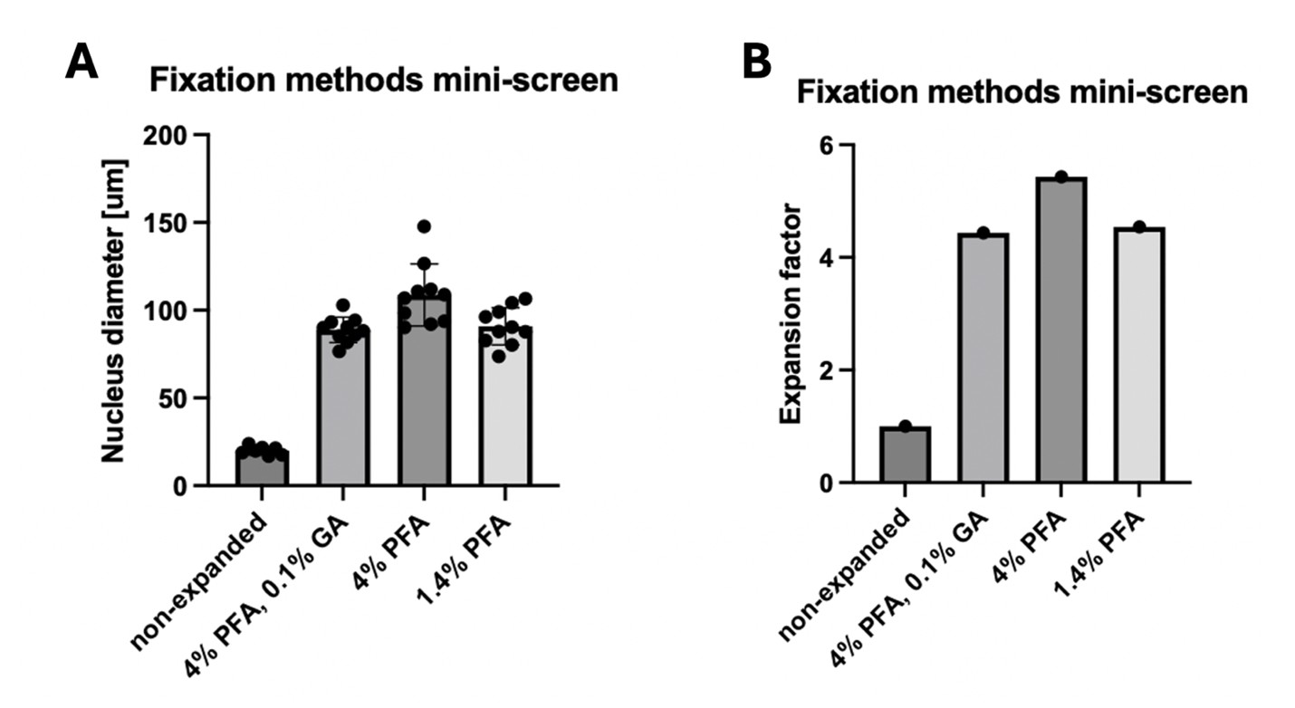
Related to the above, was the anchoring efficiency reduced only to achieve a 10x expansion factor or does this additionally affect the proteome coverage?

We solely lowered the anchoring in order to allow for higher expansion factors. In earlier pilots we performed proteomic analysis on samples that were just expanded 4x using standard TREx expansion (also using the original anchoring strategy from the TREx publication, consisting of 0.2 mg/ml AcX for overnight at RT). We presented the results of this pilot in Fig S1A. We still detected over 2,000 proteins from 10 cells, a coverage, which is highly similar to what we found in the final experiments (Figure 2F), in which the anchoring was lower yielding 10x expansion. Based on these data, we hypothesize that anchoring (and expansion factor!) has a negligible impact on protein coverage. We will clarify this in the manuscript.

d) Have the authors considered using alternative anchoring approaches, such as GMA (https://journals.plos.org/plosone/article?id=10.1371/journal.pone.0291506#pone.0291506.s001), which potentially increase the amount of sample retained in the hydrogel, thus allowing for better proteome coverage? This could be added to the discussion.

We did not use alternative anchoring approaches. We modified the TREx protocol to fit our purposes and since this was sufficient, we did not explore alternatives. However, using anchoring approaches, in which higher amounts of sample could be retained in the gel might be beneficial for the proteomics coverage. We will keep this suggestion in mind for future experiments. Thank you for the suggestion!

e) The limitation of the approach to near-2D samples should be mentioned, and alternative approaches for more 3D samples could be discussed.

The authors agree that SPEx is limited to near-2D samples at this point. We suggest that SPEx is applicable for 3D samples (e.g. in tissues) by performing cryosectioning. TREx has been shown to be compatible with sectioned tissue (Damstra et al., 2022). We will elaborate this in the discussion.

f) How are peptides that are directly anchored to the hydrogel dealt with during LC-MS/MS analysis? Are they excluded, or can they be identified during the spectral search? The latter would allow us to get a deeper structural understanding of how proteins are actually anchored into hydrogels, which so far has not been assessed.

The reviewer raises an interesting point. In general, peptides carrying the anchoring modification are analysed by LC-MS, but we did not include these specific modifications in the database search. Overall, we assumed that the labeling would be low and stochastic and hence should, if at all, only minimally affect the detection of peptides. Nevertheless, in response to the reviewers’ comment, we searched the MS data again for the crosslinking reagent linked to lysine residues. However, we could not get any confident hit for any peptide containing this modification. Since we cannot exclude that the modification precludes the identification of the corresponding peptides, we compared the number peptides generated by trypsin cleavage after arginine and lysine. As the human genome contains similar proportions of both amino acids, one would expect similar numbers of both peptide types being identified. Any modifications of lysine by the anchoring reagent used, would prevent tryptic cleavage and thus reduce the number of lysine peptides. As shown in Author response image 2, the number of lysine terminating is only slightly lower compared to arginine terminating peptides. Notably, the proteomics results of a different fixed human tissue sample directly extracted by laser capture micro dissection without expansion showed a very similar lysine to arginine peptide ratio. This indicates that the large majority of lysine residues is not modified and affected by the hydrogel anchoring.

Author response image 2.

Number of peptides identified either terminating with lysine (K) or arginine (R) across all samples shown in Figure 5F.

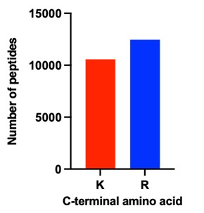
An alternative approach to address this question would be to investigate if the peptide coverage of proteins detected by SPEx is enriched for peptides representing the folded core of proteins as opposed to the surface-exposed regions, which likely get more anchored into the hydrogel.

Because of the negligible amounts of modified peptides, we did not investigate this potential bias of surface-exposed versus folded-core peptides.

g) Same question regarding peptides with NHS labeling. Can they be identified, or do they just compete for ionization and thus negatively affect coverage and dynamic range of the LC-MS/MS approach?

The reviewer raises a similar point as above for another lysine labeling used during the SPEx protocol. Again, we specifically looked for this modification by re-searching the raw MS data, but still could not identify any peptides, carrying this modification on a lysine residue. Even though we cannot exclude that this rather large modification prevents detection, considering the high number of lysine terminating peptides in our dataset (see Figure 2), we would expect that also this labeling step is stochastic and affects only a minor proportion of the proteins.

h) How are the primary and secondary antibodies affecting the proteomics analysis identified as contaminants?

We thank the reviewer for this comment. Since antibodies bind to proteins in a non-covalent manner, they will be released during the denaturing steps of the protocol. Of course, the antibodies will stay in the sample, be digested and analyzed and could, if very abundant, affect the analysis of the proteins from the samples. To check this possibility, we re-searched the MS data including the sequences of the antibodies used. To our surprise, we could not detect any peptides of these antibodies. This suggests that the concentrations of the antibodies used are much lower than those of the sample proteins and thus should not have any impact on the proteomics results.  We interpret this result also as a benefit of our method compared to organellar-IP.

i) Have the authors observed differences in proteomics coverage of only antibody vs NHS-labeling? Depending on the questions above, could pure antibody-based labeling increase proteomic coverage?

We did not perform this comparative analysis, since we always used NHS dyes. In the experiments presented in this manuscript, NHS dyes allowed easy visualization of the whole cell without the use of antibodies. This NHS staining was essential for this particular setup for sample acquisition. We cut out entire cells, cells lacking the nucleus and cells lacking the Golgi apparatus, which served as critical controls. However, other ways of detecting cell boundaries could be used to avoid NHS staining. As shown above, both, the anchor and NHS labeling are likewise sparse and stochastic. Moreover, we could not detect any impact of the antibody labeling to our results. Thus, we assume that both labeling procedures could be used.

Reviewer #2 (Public review):

Summary:

This study introduces a method that combines physical expansion of cells, imaging-guided isolation of defined regions, and protein identification to enable compartment-resolved analysis of protein composition at the subcellular scale. The authors aim to address a central limitation in existing approaches, namely the loss of spatial information during sample preparation or the indirect nature of proximity-based labeling methods. Using several cellular compartments as examples, they demonstrate that their approach can recover compartment-enriched protein sets and identify candidate proteins with previously unassigned localization.

Strengths:

A major strength of this work is the conceptual simplicity and accessibility of the approach. By combining established techniques in a modular way, the method avoids the need for genetic manipulation or specialized labeling strategies, making it broadly adaptable across experimental systems. The ability to directly select regions of interest based on imaging represents a clear advantage over indirect enrichment strategies and allows flexible targeting of both membrane-bound and non-membrane-bound compartments.

The experimental design is also a strong aspect of the study. The use of complementary comparison strategies-analyzing isolated compartments alongside matched "subtracted" controls-provides an internal framework for assessing enrichment and depletion, increasing confidence in spatial assignment. The application of the method across multiple organelles of different sizes and properties demonstrates versatility, and the reported specificity for several compartments is encouraging. In particular, the ability to profile small and biochemically challenging structures highlights a potentially important niche for the approach.

Weaknesses:

Despite these strengths, several methodological limitations constrain the interpretation of the results. The most important relates to spatial accuracy in three dimensions. While lateral resolution is improved through physical expansion, the lack of depth resolution introduces uncertainty regarding contributions from structures above and below the selected region. Although the authors argue that this does not substantially affect specificity, the current evidence is largely indirect, and a more rigorous quantification of potential contamination would strengthen this conclusion.

Quantitative interpretation also remains challenging. Because the measurements reflect total protein abundance rather than local concentration, differences in compartment size and protein density can influence enrichment values, particularly for small structures embedded within larger volumes. This issue is evident in the analysis of smaller compartments and complicates direct comparison across conditions. Additional normalization or modeling would help clarify how to interpret these measurements.

Another limitation concerns variability in the expansion process and its downstream consequences. Differences in expansion factor across samples may affect the definition of regions of interest and introduce variability in sampling, yet the impact of this variability is not fully explored. Similarly, the use of a modified chemical treatment to preserve proteins for downstream analysis is central to the workflow but is not extensively validated with respect to preservation of spatial organization.

While the identification of previously unannotated proteins is an appealing aspect of the study, validation is limited to a small number of examples, and broader support from independent datasets or literature context is lacking. In addition, the study primarily focuses on steady-state measurements in a single cell type, and therefore does not yet demonstrate the ability of the method to capture dynamic or condition-dependent changes in protein localization.

Finally, the positioning of the method relative to existing approaches could be more clearly articulated. Although qualitative comparisons are provided, a more systematic and quantitative benchmarking against alternative strategies would help readers better understand the specific advantages and trade-offs.

We thank the reviewer for the careful evaluation of the manuscript and for the constructive feedback. We think the reviewer raises valid points and will address them in the revised manuscript.

Reviewer #3 (Public review):

Franziscus et al. describe an elegant approach for spatially specific proteome analysis. To achieve this, they expand fixed cells and subsequently use a laser to micro-dissect a region of interest, which is then analyzed by mass spectrometry.

They demonstrate the effectiveness of their approach by analyzing the nucleus, nucleolus, and the Golgi, and benchmark their hits against previous datasets for these organelles.

The manuscript is very well written and nicely guides the reader through the applied methods. The presented data is convincing, and I do not see the need for additional experimental verification of the protocol. The only minor concern is the novelty of the method and the presentation. A combination of expansion, laser microdissection, and proteomics has been applied in the past (PMID: 36450705, PMID: 39477916). In the manuscript, one of these studies is cited, though it does not become clear that this approach is already described. However, Franziscus et al. describe the approach better and make it more accessible to the reader, especially since the other studies described this methodology in combination with tissue expansion and not in combination with single cell expansion as it is done here. I would ask the authors to be clearer in the introduction about what others have already done and what their contribution is here. In general, I am convinced that the community will benefit from the presented protocol to analyze organelle proteomics in detail.

We thank the reviewer for the careful evaluation of our manuscript and overwhelmingly positive assessment. We apologize for the omission of the mentioned citations, and will adjust the introduction to make it clearer what has already been done and what the advance our method provides.

References

Damstra HG, Mohar B, Eddison M, Akhmanova A, Kapitein LC, Tillberg PW. 2022. Visualizing cellular and tissue ultrastructure using Ten-fold Robust Expansion Microscopy (TREx). eLife 11:e73775. DOI: https://doi.org/10.7554/eLife.73775

Gambarotto D, Hamel V, Guichard P. 2021. Ultrastructure expansion microscopy (U-ExM). Methods in Cell Biology 161:57–81. DOI: https://doi.org/10.1016/bs.mcb.2020.05.006, PMID: 33478697

Liffner B, Silva TLA e., Vega-Rodriguez J, Absalon S. 2024. Mosquito Tissue Ultrastructure-Expansion Microscopy (MoTissU-ExM) enables ultrastructural and anatomical analysis of malaria parasites and their mosquito. BMC Methods 1:13. DOI: https://doi.org/10.1186/s44330-024-00013-4

If accounts can be suspended based on violent behavior such as threats, sexism or perhaps even inappropriate content or posts, what stops AI from being limited on these sites? In the last year a conversation around X's Grok AI supports these issues as many users were requesting inappropriate content from the model, in which Grok delivered via anti-semitic text to graphic sexual photos that violated X's terms of service. The intersection of AI and human bias is dangerous and subject to regulation.

If AI is a for profit for research pursuit, how would biases benefit any result of AI's output if it appeals to personal opinions rather than factual or impartial results? In terms of scientific research, Artificial Intelligence must uphold factual information and standards to produce quality information and cannot maintain personal biases. I can see how generative AI can possibly connect to a users outlook when conversing or creating works surrounding sensitive topics, but legally would production of biases by AI cause a dispute?

How would AI companies and their expansion intersect with politicians' and the citizen's vote on this matter? Perhaps through environmental regulations data centers can be limited in size or distance from residential areas, or would water usage be limited on a per day-year scale?

Posing a general question: how does AI energy emissions and resources compare to general energy demands for electricity? Furthermore, would an expansion of "green AI" lead to a greater expansion of renewable or green energy initiatives as a whole, or would the increased output of green energy not even compute with the consumption?

The assumption-based structure of "string predication" poses a threat of interpreting information through lenses of common results or probability rather than facts that support it.

As summarized in this passage, these LMs input cost and environmental effects are being forced upon communities that do not agree to the expansion of these models and face real results in their communities such as raised electric bills or degradation of air quality.

So the model ultimately reflects whatever story the big media chooses to tell, which we already know can be very selective. This reminds us that “what’s in the data” is also affected by “what’s ignored.”

I find it interesting that bias is introduced at multiple stages, not just one. First, not everyone has equal access to the internet. Then, the way the data is collected (like scraping it from Reddit) filters out even more voices. Finally, the "cleaning" process removes more content. Therefore, by the time the data reaches the model, the scope has been reduced by three times. It does challenge the notion that online data is “neutral” or “representative” of everyone.

This definition actually helped me understand what the core of LM really does - it's basically just predicting the next token based on what happened before (or what's around it). It doesn't sound so magical when you put it like that. I think this is directly related to the "random parrot" idea later in this article: it makes sense that if all the model does is guess the most likely next word, it doesn't actually "understand" anything. It's very good at pattern matching.

Since most internet content comes from already dominant groups, this model ends up reinforcing these same views. It's a twofold problem: not only is the data biased, but it's too large for anyone to fully inspect or fix.

All newly detected solitary gastric polyps should be resected at the time of index endoscopy to achieve both diagnostic and therapeutic goals

For polyps exceeding 20 mm, referral to an endoscopist with experience in advanced resection techniques is advised

Surveillance Recommendations for Gastric Polyps

Surveillance plans should be formulated based on the histopathological type of the polyps and surrounding gastric mucosa: [1]

Fundic gland polyps (FGPs): Non-syndromic FGPs without dysplasia do not require surveillance endoscopy. However, watchful follow-up is advised for syndromic patients with dysplastic FGPs, large polyps (>10 mm), or mucosal carpeting by polyps. [1] Hyperplastic polyps: Endoscopic resection is advised for large polyps (>10 mm). If dysplasia is noted on biopsy, periodic (yearly) surveillance is advised. Helicobacter pylori eradication can lead to regression of hyperplastic polyps. [1] Gastric adenomas: After complete resection, follow-up surveillance endoscopy should be completed at 1 year for low-grade dysplasia and 6 months for high-grade dysplasia. If the polyp is biopsied or resection is incomplete, follow-up endoscopy is advised within 3 months for high-grade dysplasia and 6 months for low-grade dysplasia. Subsequent annual follow-up is recommended to monitor for malignant changes. [1] Surrounding mucosa: Endoscopic surveillance is advised when histopathology of adjacent mucosa confirms gastric intestinal metaplasia (GIM) and/or atrophic gastritis. Biopsies from the gastric antrum and corpus should be obtained at minimum

The majority are fundic gland polyps or hyperplastic polyps, which usually are small, single or multiple. Fundic gland polyps have no malignant potential and do not usually require removal or endoscopic surveillance

20) fundic gland polyps are found or concomitant duodenal adenomas are present, the possibility of familial polyposis should be considered. Large hyperplastic polyps (> 1.0 cm) should be removed at endoscopy as they may rarely cause chronic blood loss.

Adenomatous polyps account for 10–20% of gastric polyps. They are usually solitary lesions that usually arise in a background of chronic atrophic gastritis associated with H pylori infection, which should be treated

Submucosal gastric polypoid lesions include benign gastric stromal tumors (commonly misclassified as leiomyomas) and pancreatic rests

Hyperplastic polyps are associated with chronic gastritis and Helicobacter pylori infection. Fundic gland polyps are often multiple and associated with proton pump inhibitor use or familial adenomatous polyposis

Submucosal tumors present as polypoid lesions beneath intact mucosa and require differentiation from malignant entities:

Leiomyomas: Well-circumscribed, hypodense lesions commonly in the cardia; slow-growing tumors from smooth muscle cells [1-2] Lipomas: Well-circumscribed, low-attenuation lesions composed of adipose tissue with characteristic yellowish appearance on endoscopy [1][7] Schwannomas: Rare, well-defined tumors that may show progressive enhancement; more common in females and elderly patients (age 50-60 years) [1][3] Glomus tumors: Hypervascular solitary lesions typically in the antrum [1][7] Heterotopic pancreas: Developmental anomaly appearing as polypoid lesion, commonly in the antrum

For submucosal tumors, surface biopsy may be non-diagnostic as the overlying mucosa is typically intact. [5] Endoscopic ultrasound (EUS) is valuable for characterizing submucosal lesions, determining the layer of origin, assessing size, and differentiating benign from malignant features. EUS shows characteristic patterns: lipomas appear hyperechoic in the submucosa, while leiomyomas appear hypoechoic.

Specific CT features help differentiate tumor types

MRI may be used as an adjunct, particularly for characterizing larger lesions or when CT findings are equivocal.

Malignant transformation potential varies: adenomas are precancerous and require complete removal, while hyperplastic polyps have low malignant potential except when showing dysplasia

Case#: The patient is male, 3 years and 10 months old. Ethnicity not specified

DiseaseAssertion: The patient is asserted to have CTLA-4 insufficiency.

FamilyInfo: Patient's mother has type 1 diabetes and autoimmune thyroiditis. The patient's maternal aunt has celiac disease and Lenox-Gastaut syndrome.

CasePresentingHPOs: HP:0001873 (Thombocytopenia), HP:0011947 (Respiratory tract infection), HP:0000988 (skin rash), HP:0000967 (Petechiae), HP:0034752 (Axillary lymphadenopathy), HP:0001047 (Atopic dermatitis), HP:0001903 (Anemia), HP:0012234 (Agranulocytosis),

CaseHPOFreeText: Patient had a mild upper respiratory tract infect followed by a small-spotted hemorrhagic rash and skin bruising. Physical examination was significant for punctate petechiae on skin and soft palate, as well as enlarged axillary lymph nodes bilaterally. On a subsequent visit patient was

CaseNotHPOs:

CaseNotHPOFreeText: Bone marrow biopsy did not reveal any abnormalities.

CasePreviousTesting:

GenotypingMethod:

PreviouslyPublished No prior article is known to contain information on the same proband.

Variant:

ClinVar:

gnomAD:

SupplementalData:

Case#: The patient is male, 3 years and 10 months old. Ethnicity not specified

DiseaseAssertion: The patient is asserted to have CTLA-4 insufficiency.

FamilyInfo: Patient's mother has type 1 diabetes and autoimmune thyroiditis. The patient's maternal aunt has celiac disease and Lenox-Gastaut syndrome.

CasePresentingHPOs: HP:0001873 (Thombocytopenia), HP:0011947 (Respiratory tract infection), HP:0000988 (skin rash), HP:0000967 (Petechiae), HP:0034752 (Axillary lymphadenopathy), HP:0001047 (Atopic dermatitis), HP:0001903 (Anemia), HP:0012234 (Agranulocytosis),

CaseHPOFreeText: Patient had a mild upper respiratory tract infect followed by a small-spotted hemorrhagic rash and skin bruising. Physical examination was significant for punctate petechiae on skin and soft palate, as well as enlarged axillary lymph nodes bilaterally. On a subsequent visit patient was

CaseNotHPOs:

CaseNotHPOFreeText: Bone marrow biopsy did not reveal any abnormalities.

CasePreviousTesting:

GenotypingMethod:

PreviouslyPublished No prior article is known to contain information on the same proband.

Variant:

ClinVar:

gnomAD:

SupplementalData:

Case#: The patient is male, 3 years and 10 months old. Ethnicity not specified

DiseaseAssertion: The patient is asserted to have CTLA-4 insufficiency.

FamilyInfo: Patient's mother has type 1 diabetes and autoimmune thyroiditis. The patient's maternal aunt has celiac disease and Lenox-Gastaut syndrome.

CasePresentingHPOs: HP:0001873 (Thombocytopenia), HP:0011947 (Respiratory tract infection), HP:0000988 (skin rash), HP:0000967 (Petechiae), HP:0034752 (Axillary lymphadenopathy), HP:0001047 (Atopic dermatitis), HP:0001903 (Anemia), HP:0012234 (Agranulocytosis),

CaseHPOFreeText: Patient had a mild upper respiratory tract infect followed by a small-spotted hemorrhagic rash and skin bruising. Physical examination was significant for punctate petechiae on skin and soft palate, as well as enlarged axillary lymph nodes bilaterally. On a subsequent visit patient was

CaseNotHPOs:

CaseNotHPOFreeText: Bone marrow biopsy did not reveal any abnormalities.

CasePreviousTesting:

GenotypingMethod:

PreviouslyPublished No prior article is known to contain information on the same proband.

Variant:

ClinVar:

gnomAD:

SupplementalData:

Case#: The patient is male, 3 years and 10 months old. Ethnicity not specified

DiseaseAssertion: The patient is asserted to have CTLA-4 insufficiency.

FamilyInfo: Patient's mother has type 1 diabetes and autoimmune thyroiditis. The patient's maternal aunt has celiac disease and Lenox-Gastaut syndrome.

CasePresentingHPOs: HP:0001873 (Thombocytopenia), HP:0011947 (Respiratory tract infection), HP:0000988 (skin rash), HP:0000967 (Petechiae), HP:0034752 (Axillary lymphadenopathy), HP:0001047 (Atopic dermatitis), HP:0001903 (Anemia), HP:0012234 (Agranulocytosis),

CaseHPOFreeText: Patient had a mild upper respiratory tract infect followed by a small-spotted hemorrhagic rash and skin bruising. Physical examination was significant for punctate petechiae on skin and soft palate, as well as enlarged axillary lymph nodes bilaterally. On a subsequent visit patient was

CaseNotHPOs:

CaseNotHPOFreeText: Bone marrow biopsy did not reveal any abnormalities.

CasePreviousTesting:

GenotypingMethod:

PreviouslyPublished No prior article is known to contain information on the same proband.

Variant:

ClinVar:

gnomAD:

SupplementalData:

Case#: The patient is male, 3 years and 10 months old. Ethnicity not specified

DiseaseAssertion: The patient is asserted to have CTLA-4 insufficiency.

FamilyInfo: Patient's mother has type 1 diabetes and autoimmune thyroiditis. The patient's maternal aunt has celiac disease and Lenox-Gastaut syndrome.

CasePresentingHPOs: HP:0001873 (Thombocytopenia), HP:0011947 (Respiratory tract infection), HP:0000988 (skin rash), HP:0000967 (Petechiae), HP:0034752 (Axillary lymphadenopathy), HP:0001047 (Atopic dermatitis), HP:0001903 (Anemia), HP:0012234 (Agranulocytosis),

CaseHPOFreeText: Patient had a mild upper respiratory tract infect followed by a small-spotted hemorrhagic rash and skin bruising. Physical examination was significant for punctate petechiae on skin and soft palate, as well as enlarged axillary lymph nodes bilaterally. On a subsequent visit patient was

CaseNotHPOs:

CaseNotHPOFreeText: Bone marrow biopsy did not reveal any abnormalities.

CasePreviousTesting:

GenotypingMethod:

PreviouslyPublished No prior article is known to contain information on the same proband.

Variant:

ClinVar:

gnomAD:

SupplementalData:

GigaScience has a strict policy on publishing open source software, and while the GitLab repository isn't yet public you can see the original codebase under a GPL 3.0 license here: https://github.com/gigascience/gigadb-website/

The original GigaScience team did not start working on the project until late 2010, and the database launched in June 2011 (which was prior to the launch of the journal in July 2012). See the announcement blog blog https://doi.org/10.59350/r3pva-55v87

And the GigaDB launch Edtorial

Sneddon TP, Li P, Edmunds SC. GigaDB: announcing the GigaScience database. Gigascience. 2012 Jul 12;1(1):11. https://doi.org/10.1186/2047-217X-1-11

three major forms of managed care: Purpose is to control cost.

fee-for-service practice with utilization review- whether private insurance company or government agency) assumes the power to authorize or deny payment for expensive medical interventions (hospital admissions, extra hospital days, and surgeries).

preferred provider organizations (PPOs)- insurers contract with a limited number of physicians and hospitals who agree to care for patients, usually on a discounted fee-for-service or, for hospitals, a per diem basis, with utilization review (the insurer authorizing or denying payment for services deemed unnecessary).

health maintenance organizations (HMOs)- are required (except in emergencies) to receive their care from physicians and hospitals within that HMO. -Some HMOs pay physicians and hospitals by more highly bundled units of payment.

The physician or hospital is paid a fee for each office visit, ECG, intravenous fluid, or other service or supply provided.

the payment of a fee or grant to a doctor

this seems to need more digging into!

make it clearer that this is a living document, under active adjustment, and responsive to suggestions

Put the 'which animal products, and their welfare burden' as the fourth item (d instead of c), because that weighting acts on 'the net reduction in production of each animal product'

I'd make (c) 'how much the production of each animal product adjusts in response in market equilibrium' [tooltip: this may not be 1 for 1, e.g., with scarcity or increasing marginal costs, if some consumers purchase less of an animal product, other consumers may pick up the slack. For example, with an ~inelastic supply of wild fish, if some consumers switch to plant-based equivalents, this may drive prices down, getting other consumers to buy more wild fish]

"make it a relatively tractable" ('most' is too conclusive)

how large is the plant-based meat market today

I don't see how this follows -- if 50%+ rate it as as good or better than the conventional product, that should imply that the median consumer finds it 'as good or better'. Correct?

This wotks better as a note than a quantitative report. Same for "Most favorable public category result" -- perhaps put those at the bottom in a few sentences rather than a tabular format

I don't think this is 'the strongest evidence'. To me the GFI Germany/UK surveys seems particular strong at least for the EU.

which survey? a US-one right? THe GFI Europe one asked about actual consumption it seems

Letter to Parliament in which minister for digital economy acts on advice of the investment authority and forbids the sale of Solvinity to US Kyndryl, due to high risk to Dutch digital sovereignty