Author response:
eLife assessment
This potentially useful study involves neuro-imaging and electrophysiology in a small cohort of congenital cataract patients after sight recovery and age-matched control participants with normal sight. It aims to characterize the effects of early visual deprivation on excitatory and inhibitory balance in the visual cortex. While the findings are taken to suggest the existence of persistent alterations in Glx/GABA ratio and aperiodic EEG signals, the evidence supporting these claims is incomplete. Specifically, small sample sizes, lack of a specific control cohort, and other methodological limitations will likely restrict the usefulness of the work, with relevance limited to scientists working in this particular subfield.
As pointed out in the public reviews, there are only very few human models which allow for assessing the role of early experience on neural circuit development. While the prevalent research in permanent congenital blindness reveals the response and adaptation of the developing brain to an atypical situation (blindness), research in sight restoration addresses the question of whether and how atypical development can be remediated if typical experience (vision) is restored. The literature on the role of visual experience in the development of E/I balance in humans, assessed via Magnetic Resonance Spectroscopy (MRS), has been limited to a few studies on congenital permanent blindness. Thus, we assessed sight recovery individuals with a history of congenital blindness, as limited evidence from other researchers indicated that the visual cortex E/I ratio might differ compared to normally sighted controls.
Individuals with total bilateral congenital cataracts who remained untreated until later in life are extremely rare, particularly if only carefully diagnosed patients are included in a study sample. A sample size of 10 patients is, at the very least, typical of past studies in this population, even for exclusively behavioral assessments. In the present study, in addition to behavioral assessment as an indirect measure of sensitive periods, we investigated participants with two neuroimaging methods (Magnetic Resonance Spectroscopy and electroencephalography) to directly assess the neural correlates of sensitive periods in humans. The electroencephalography data allowed us to link the results of our small sample to findings documented in large cohorts of both, sight recovery individuals and permanently congenitally blind individuals. As pointed out in a recent editorial recommending an “exploration-then-estimation procedure,” (“Consideration of Sample Size in Neuroscience Studies,” 2020), exploratory studies like ours provide crucial direction and specific hypotheses for future work.
We included an age-matched sighted control group recruited from the same community, measured in the same scanner and laboratory, to assess whether early experience is necessary for a typical excitatory/inhibitory (E/I) ratio to emerge in adulthood. The present findings indicate that this is indeed the case. Based on these results, a possible question to answer in future work, with individuals who had developmental cataracts, is whether later visual deprivation causes similar effects. Note that even if visual deprivation at a later stage in life caused similar effects, the current results would not be invalidated; by contrast, they are essential to understand future work on late (permanent or transient) blindness.
Thus, we think that the present manuscript has far reaching implications for our understanding of the conditions under which E/I balance, a crucial characteristic of brain functioning, emerges in humans.
Finally, our manuscript is one of the first few studies which relates MRS neurotransmitter concentrations to parameters of EEG aperiodic activity. Since present research has been using aperiodic activity as a correlate of the E/I ratio, and partially of higher cognitive functions, we think that our manuscript additionally contributes to a better understanding of what might be measured with aperiodic neurophysiological activity.
Public Reviews:
Reviewer #1 (Public Review):
Summary:
In this human neuroimaging and electrophysiology study, the authors aimed to characterize the effects of a period of visual deprivation in the sensitive period on excitatory and inhibitory balance in the visual cortex. They attempted to do so by comparing neurochemistry conditions ('eyes open', 'eyes closed') and resting state, and visually evoked EEG activity between ten congenital cataract patients with recovered sight (CC), and ten age-matched control participants (SC) with normal sight.
First, they used magnetic resonance spectroscopy to measure in vivo neurochemistry from two locations, the primary location of interest in the visual cortex, and a control location in the frontal cortex. Such voxels are used to provide a control for the spatial specificity of any effects because the single-voxel MRS method provides a single sampling location. Using MR-visible proxies of excitatory and inhibitory neurotransmission, Glx and GABA+ respectively, the authors report no group effects in GABA+ or Glx, no difference in the functional conditions 'eyes closed' and 'eyes open'. They found an effect of the group in the ratio of Glx/GABA+ and no similar effect in the control voxel location. They then performed multiple exploratory correlations between MRS measures and visual acuity, and reported a weak positive correlation between the 'eyes open' condition and visual acuity in CC participants.
The same participants then took part in an EEG experiment. The authors selected only two electrodes placed in the visual cortex for analysis and reported a group difference in an EEG index of neural activity, the aperiodic intercept, as well as the aperiodic slope, considered a proxy for cortical inhibition. They report an exploratory correlation between the aperiodic intercept and Glx in one out of three EEG conditions.
The authors report the difference in E/I ratio, and interpret the lower E/I ratio as representing an adaptation to visual deprivation, which would have initially caused a higher E/I ratio. Although intriguing, the strength of evidence in support of this view is not strong. Amongst the limitations are the low sample size, a critical control cohort that could provide evidence for a higher E/I ratio in CC patients without recovered sight for example, and lower data quality in the control voxel.
Strengths of study:
How sensitive period experience shapes the developing brain is an enduring and important question in neuroscience. This question has been particularly difficult to investigate in humans. The authors recruited a small number of sight-recovered participants with bilateral congenital cataracts to investigate the effect of sensitive period deprivation on the balance of excitation and inhibition in the visual brain using measures of brain chemistry and brain electrophysiology. The research is novel, and the paper was interesting and well-written.
Limitations:
(1.1) Low sample size. Ten for CC and ten for SC, and a further two SC participants were rejected due to a lack of frontal control voxel data. The sample size limits the statistical power of the dataset and increases the likelihood of effect inflation.
Applying strict criteria, we only included individuals who were born with no patterned vision in the CC group. The population of individuals who have remained untreated past infancy is small in India, despite a higher prevalence of childhood cataract than Germany. Indeed, from the original 11 CC and 11 SC participants tested, one participant each from the CC and SC group had to be rejected, as their data had been corrupted, resulting in 10 participants in each group.
It was a challenge to recruit participants from this rare group with no history of neurological diagnosis/intake of neuromodulatory medications, who were able and willing to undergo both MRS and EEG. For this study, data collection took more than 1.5 years.
We took care of the validity of our results with two measures; first, assessed not just MRS, but additionally, EEG measures of E/I ratio. The latter allowed us to link results to a larger population of CC individuals, that is, we replicated the results of a larger group of 38 individuals (Ossandón et al., 2023) in our sub-group.
Second, we included a control voxel. As predicted, all group effects were restricted to the occipital voxel.
(1.2) Lack of specific control cohort. The control cohort has normal vision. The control cohort is not specific enough to distinguish between people with sight loss due to different causes and patients with congenital cataracts with co-morbidities. Further data from more specific populations, such as patients whose cataracts have not been removed, with developmental cataracts, or congenitally blind participants, would greatly improve the interpretability of the main finding. The lack of a more specific control cohort is a major caveat that limits a conclusive interpretation of the results.
The existing work on visual deprivation and neurochemical changes, as assessed with MRS, has been limited to permanent congenital blindness. In fact, most of the studies on permanent blindness included only congenitally blind or early blind humans (Coullon et al., 2015; Weaver et al., 2013), or, in separate studies, only late-blind individuals (Bernabeu et al., 2009). Thus, accordingly, we started with the most “extreme” visual deprivation model, sight recovery after congenital blindness. If we had not observed any group difference compared to normally sighted controls, investigating other groups might have been trivial. Based on our results, subsequent studies in late blind individuals, and then individuals with developmental cataracts, can be planned with clear hypotheses.
(1.3) MRS data quality differences. Data quality in the control voxel appears worse than in the visual cortex voxel. The frontal cortex MRS spectrum shows far broader linewidth than the visual cortex (Supplementary Figures). Compared to the visual voxel, the frontal cortex voxel has less defined Glx and GABA+ peaks; lower GABA+ and Glx concentrations, lower NAA SNR values; lower NAA concentrations. If the data quality is a lot worse in the FC, then small effects may not be detectable.
Worse data quality in the frontal than the visual cortex has been repeatedly observed in the MRS literature, attributable to magnetic field distortions (Juchem & Graaf, 2017) resulting from the proximity of the region to the sinuses (recent example: (Rideaux et al., 2022)). Nevertheless, we chose the frontal control region rather than a parietal voxel, given the potential neurochemical changes in multisensory regions of the parietal cortex due to blindness. Such reorganization would be less likely in frontal areas associated with higher cognitive functions. Further, prior MRS studies of the visual cortex have used the frontal cortex as a control region as well (Pitchaimuthu et al., 2017; Rideaux et al., 2022).
In the present study, we checked that the frontal cortex datasets for Glx and GABA+ concentrations were of sufficient quality: the fit error was below 8.31% in both groups (Supplementary Material S3). For reference, Mikkelsen et al. reported a mean GABA+ fit error of 6.24 +/- 1.95% from a posterior cingulate cortex voxel across 8 GE scanners, using the Gannet pipeline. No absolute cutoffs have been proposed for fit errors. However, MRS studies in special populations (I/E ratio assessed in narcolepsy (Gao et al., 2024), GABA concentration assessed in Autism Spectrum Disorder (Maier et al., 2022)) have used frontal cortex data with a fit error of <10% to identify differences between cohorts (Gao et al., 2024; Pitchaimuthu et al., 2017). Based on the literature, MRS data from the frontal voxel of the present study would have been of sufficient quality to uncover group differences.
In the revised manuscript, we will add the recently published MRS quality assessment form to the supplementary materials. Additionally, we would like to allude to our apriori prediction of group differences for the visual cortex, but not for the frontal cortex voxel.
(1.4) Because of the direction of the difference in E/I, the authors interpret their findings as representing signatures of sight improvement after surgery without further evidence, either within the study or from the literature. However, the literature suggests that plasticity and visual deprivation drive the E/I index up rather than down. Decreasing GABA+ is thought to facilitate experience-dependent remodelling. What evidence is there that cortical inhibition increases in response to a visual cortex that is over-sensitised due to congenital cataracts? Without further experimental or literature support this interpretation remains very speculative.
Indeed, higher inhibition was not predicted, which we attempt to reconcile in our discussion section. We base our discussion mainly on the non-human animal literature, which has shown evidence of homeostatic changes after prolonged visual deprivation in the adult brain (Barnes et al., 2015). It is also interesting to note that after monocular deprivation in adult humans, resting GABA+ levels decreased in the visual cortex (Lunghi et al., 2015). Assuming that after delayed sight restoration, adult neuroplasticity mechanisms must be employed, these studies would predict a “balancing” of the increased excitatory drive following sight restoration by a commensurate increase in inhibition (Keck et al., 2017). Additionally, the EEG results of the present study allowed for speculation regarding the underlying neural mechanisms of an altered E/I ratio. The aperiodic EEG activity suggested higher spontaneous spiking (increased intercept) and increased inhibition (steeper aperiodic slope between 1-20 Hz) in CC vs SC individuals (Ossandón et al., 2023).
In the revised manuscript, we will more clearly indicate that these speculations are based primarily on non-human animal work, due to the lack of human studies on the subject.
(1.5) Heterogeneity in the patient group. Congenital cataract (CC) patients experienced a variety of duration of visual impairment and were of different ages. They presented with co-morbidities (absorbed lens, strabismus, nystagmus). Strabismus has been associated with abnormalities in GABAergic inhibition in the visual cortex. The possible interactions with residual vision and confounds of co-morbidities are not experimentally controlled for in the correlations, and not discussed.
The goal of the present study was to assess whether we would observe changes in E/I ratio after restoring vision at all. We would not have included patients without nystagmus in the CC group of the present study, since it would have been unlikely that they experienced congenital patterned visual deprivation. Amongst diagnosticians, nystagmus or strabismus might not be considered genuine “comorbidities” that emerge in people with congenital cataracts. Rather, these are consequences of congenital visual deprivation, which we employed as diagnostic criteria. Similarly, absorbed lenses are clear signs that cataracts were congenital. As in other models of experience dependent brain development (e.g. the extant literature on congenital permanent blindness, including anophthalmic individuals (Coullon et al., 2015; Weaver et al., 2013), some uncertainty remains regarding whether the (remaining, in our case) abnormalities of the eye, or the blindness they caused, are the factors driving neural changes. In case of people with reversed congenital cataracts, at least the retina is considered to be intact, as they would otherwise not receive cataract removal surgery.
However, we consider it unlikely that strabismus caused the group differences, because the present study shows group differences in the Glx/GABA+ ratio at rest, regardless of eye opening or eye closure, for which strabismus would have caused distinct effects. By contrast, the link between GABA concentration and, for example, interocular suppression in strabismus, have so far been documented during visual stimulation (Mukerji et al., 2022; Sengpiel et al., 2006), and differed in direction depending on the amblyopic vs. non-amblyopic eye. Further, one MRS study did not find group differences in GABA concentration between the visual cortices of 16 amblyopic individuals and sighted controls (Mukerji et al., 2022), supporting that the differences in Glx/GABA+ concentration which we observed were driven by congenital deprivation, and not amblyopia-associated visual acuity or eye movement differences.
In the revised manuscript, we will discuss the inclusion criteria in more detail, and the aforementioned reasons why our data remains interpretable.
(1.6) Multiple exploratory correlations were performed to relate MRS measures to visual acuity (shown in Supplementary Materials), and only specific ones were shown in the main document. The authors describe the analysis as exploratory in the 'Methods' section. Furthermore, the correlation between visual acuity and E/I metric is weak, and not corrected for multiple comparisons. The results should be presented as preliminary, as no strong conclusions can be made from them. They can provide a hypothesis to test in a future study.
In the revised manuscript, we will clearly indicate that the exploratory correlation analyses are reported to put forth hypotheses for future studies.
(1.7) P.16 Given the correlation of the aperiodic intercept with age ("Age negatively correlated with the aperiodic intercept across CC and SC individuals, that is, a flattening of the intercept was observed with age"), age needs to be controlled for in the correlation between neurochemistry and the aperiodic intercept. Glx has also been shown to negatively correlate with age.
The correlation between chronological age and aperiodic intercept was observed across groups, but the correlation between Glx and the intercept of the aperiodic EEG activity was seen only in the CC group, even though the SC group was matched for age. Thus, such a correlation was very unlikely to be predominantly driven by an effect of chronological age.
In the revised manuscript, we will add the linear regressions with age as a covariate included below, for the relationship between aperiodic intercept and Glx concentration in the CC group.
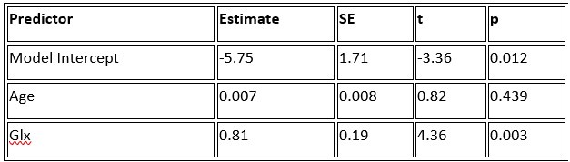
a. A linear regression was conducted within the CC group to predict the intercept during visual stimulation, based on age and visual cortex Glx concentration. The results of the regression analysis indicated that the model explained a significant proportion of the variance in the aperiodic intercept, 𝑅2\=0.82_, t_(2,7)=16.1_, 𝑝=0.0024._ Note that the coefficient for age was not significant, 𝛽=0.007, t(7)=0.82, 𝑝=0.439. The regression coefficients and their respective statistics are presented in Author response table 1.
Author response table 1.
Regression Analysis Summary for Predicting Aperiodic Intercept (Visual Stimulation) in the CC group
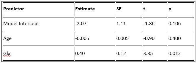
b. A linear regression was conducted to predict the intercept during eye opening at rest, based on age and visual cortex Glx concentration. The results of the regression analysis indicated that the model explained a significant proportion of the variance in the aperiodic intercept, 𝑅2\=0.842_, t_(2,7)=18.6, 𝑝=0.00159_._ Note that the coefficient for age was not significant, 𝛽=−0.005, t(7)=−0.90, 𝑝=0.400. The regression coefficients and their respective statistics are presented in Author response table 2.
Author response table 2.
Regression Analysis Summary for Predicting Aperiodic Intercept (Eyes Open) in the CC group
c. Given that the Glx coefficient is significant in both models and age does not significantly predict either outcome, it can be concluded that Glx independently predicts the intercept of the aperiodic intercept.
(1.8) Multiple exploratory correlations were performed to relate MRS to EEG measures (shown in Supplementary Materials), and only specific ones were shown in the main document. Given the multiple measures from the MRS, the correlations with the EEG measures were exploratory, as stated in the text, p.16, and in Figure 4. Yet the introduction said that there was a prior hypothesis "We further hypothesized that neurotransmitter changes would relate to changes in the slope and intercept of the EEG aperiodic activity in the same subjects." It would be great if the text could be revised for consistency and the analysis described as exploratory.
In the revised manuscript, we will improve the phrasing. We consider the correlation analyses as exploratory due to our sample size and the absence of prior work. However, we did hypothesize that both MRS and EEG markers would concurrently be altered in CC vs SC individuals.
(1.9) The analysis for the EEG needs to take more advantage of the available data. As far as I understand, only two electrodes were used, yet far more were available as seen in their previous study (Ossandon et al., 2023). The spatial specificity is not established. The authors could use the frontal cortex electrode (FP1, FP2) signals as a control for spatial specificity in the group effects, or even better, all available electrodes and correct for multiple comparisons. Furthermore, they could use the aperiodic intercept vs Glx in SC to evaluate the specificity of the correlation to CC.
The aperiodic intercept and slope did not differ between CC and SC individuals for Fp1 and Fp2, suggesting the spatial specificity of the results. In the revised manuscript, we will add this analysis to the supplementary material.
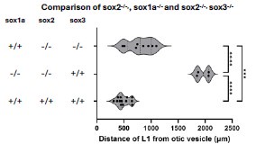
Author response image 1.
Aperiodic intercept (top) and slope (bottom) for congenital cataract-reversal (CC, red) and age-matched normally sighted control (SC, blue) individuals. Distributions of these parameters are displayed as violin plots for three conditions; at rest with eyes closed (EC), at rest with eyes open (EO) and during visual stimulation (LU). Aperiodic parameters were calculated across electrodes Fp1 and Fp2. Solid black lines indicate mean values, dotted black lines indicate median values. Coloured lines connect values of individual participants across conditions.
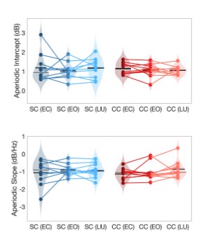
Further, Glx concentration in the visual cortex did not correlate with the aperiodic intercept in the SC group (Figure 4), suggesting that this relationship was indeed specific to the CC group.
The data from all electrodes has been analyzed and published in other studies as well (Pant et al., 2023; Ossandón et al., 2023).
Reviewer #2 (Public Review):
Summary:
The manuscript reports non-invasive measures of activity and neurochemical profiles of the visual cortex in congenitally blind patients who recovered vision through the surgical removal of bilateral dense cataracts. The declared aim of the study is to find out how restoring visual function after several months or years of complete blindness impacts the balance between excitation and inhibition in the visual cortex.
Strengths:
The findings are undoubtedly useful for the community, as they contribute towards characterising the many ways this special population differs from normally sighted individuals. The combination of MRS and EEG measures is a promising strategy to estimate a fundamental physiological parameter - the balance between excitation and inhibition in the visual cortex, which animal studies show to be heavily dependent upon early visual experience. Thus, the reported results pave the way for further studies, which may use a similar approach to evaluate more patients and control groups.
Weaknesses:
(2.1) The main issue is the lack of an appropriate comparison group or condition to delineate the effect of sight recovery (as opposed to the effect of congenital blindness). Few previous studies suggested an increased excitation/Inhibition ratio in the visual cortex of congenitally blind patients; the present study reports a decreased E/I ratio instead. The authors claim that this implies a change of E/I ratio following sight recovery. However, supporting this claim would require showing a shift of E/I after vs. before the sight-recovery surgery, or at least it would require comparing patients who did and did not undergo the sight-recovery surgery (as common in the field).
Longitudinal studies would indeed be the best way to test the hypothesis that the lower E/I ratio in the CC group observed by the present study is a consequence of sight restoration. However, longitudinal studies involving neuroimaging are an effortful challenge, particularly in research conducted outside of major developed countries and dedicated neuroimaging research facilities. Crucially, however, had CC and SC individuals, as well as permanently congenitally blind vs SC individuals (Coullon et al., 2015; Weaver et al., 2013), not differed on any neurochemical markers, such a longitudinal study might have been trivial. Thus, in order to justify and better tailor longitudinal studies, cross-sectional studies are an initial step.
(2.2) MR Spectroscopy shows a reduced GLX/GABA ratio in patients vs. sighted controls; however, this finding remains rather isolated, not corroborated by other observations. The difference between patients and controls only emerges for the GLX/GABA ratio, but there is no accompanying difference in either the GLX or the GABA concentrations. There is an attempt to relate the MRS data with acuity measurements and electrophysiological indices, but the explorative correlational analyses do not help to build a coherent picture. A bland correlation between GLX/GABA and visual impairment is reported, but this is specific to the patients' group (N=10) and would not hold across groups (the correlation is positive, predicting the lowest GLX/GABA ratio values for the sighted controls - the opposite of what is found). There is also a strong correlation between GLX concentrations and the EEG power at the lowest temporal frequencies. Although this relation is intriguing, it only holds for a very specific combination of parameters (of the many tested): only with eyes open, only in the patient group.
We interpret these findings differently, that is, in the context of experiments from non-human animals and the larger MRS literature.
Homeostatic control of E/I balance assumes that the ratio of excitation (reflected here by Glx) and inhibition (reflected here by GABA+) is regulated. Like prior work (Gao et al., 2024, 2024; Narayan et al., 2022; Perica et al., 2022; Steel et al., 2020; Takado et al., 2022; Takei et al., 2016), we assumed that the ratio of Glx/GABA+ is indicative of E/I balance rather than solely the individual neurotransmitter levels. One of the motivations for assessing the ratio vs the absolute concentration is that as per the underlying E/I balance hypothesis, a change in excitation would cause a concomitant change in inhibition, and vice versa, which has been shown in non-human animal work (Fang et al., 2021; Haider et al., 2006; Tao & Poo, 2005) and modeling research (Vreeswijk & Sompolinsky, 1996; Wu et al., 2022). Importantly, our interpretation of the lower E/I ratio is not just from the Glx/GABA+ ratio, but additionally, based on the steeper EEG aperiodic slope (1-20 Hz).
As in the discussion section and response 1.4, we did not expect to see a lower Glx/GABA+ ratio in CC individuals. We discuss the possible reasons for the direction of the correlation with visual acuity and aperiodic offset during passive visual stimulation, and offer interpretations and (testable) hypotheses.
We interpret the direction of the Glx/GABA+ correlation with visual acuity to imply that patients with highest (compensatory) balancing of the consequences of congenital blindness (hyperexcitation), in light of visual stimulation, are those who recover best. Note, the sighted control group was selected based on their “normal” vision. Thus, clinical visual acuity measures are not expected to sufficiently vary, nor have the resolution to show strong correlations with neurophysiological measures. By contrast, the CC group comprised patients highly varying in visual outcomes, and thus were ideal to investigate such correlations.
This holds for the correlation between Glx and the aperiodic intercept, as well. Previous work has suggested that the intercept of the aperiodic activity is associated with broadband spiking activity in neural circuits (Manning et al., 2009). Thus, an atypical increase of spiking activity during visual stimulation, as indirectly suggested by “old” non-human primate work on visual deprivation (Hyvärinen et al., 1981) might drive a correlation not observed in healthy populations.
In the revised manuscript, we will more clearly indicate in the discussion that these are possible post-hoc interpretations. We argue that given the lack of such studies in humans, it is all the more important that extant data be presented completely, even if the direction of the effects are not as expected.
(2.3) For these reasons, the reported findings do not allow us to draw firm conclusions on the relation between EEG parameters and E/I ratio or on the impact of early (vs. late) visual experience on the excitation/inhibition ratio of the human visual cortex.
Indeed, the correlations we have tested between the E/I ratio and EEG parameters were exploratory, and have been reported as such. The goal of our study was not to compare the effects of early vs. late visual experience. The goal was to study whether early visual experience is necessary for a typical E/I ratio in visual neural circuits. We provided clear evidence in favor of this hypothesis. Thus, the present results suggest the necessity of investigating the effects of late visual deprivation. In fact, such research is missing in permanent blindness as well.
Reviewer #3 (Public Review):
This manuscript examines the impact of congenital visual deprivation on the excitatory/inhibitory (E/I) ratio in the visual cortex using Magnetic Resonance Spectroscopy (MRS) and electroencephalography (EEG) in individuals whose sight was restored. Ten individuals with reversed congenital cataracts were compared to age-matched, normally sighted controls, assessing the cortical E/I balance and its interrelationship to visual acuity. The study reveals that the Glx/GABA ratio in the visual cortex and the intercept and aperiodic signal are significantly altered in those with a history of early visual deprivation, suggesting persistent neurophysiological changes despite visual restoration.
My expertise is in EEG (particularly in the decomposition of periodic and aperiodic activity) and statistical methods. I have several major concerns in terms of methodological and statistical approaches along with the (over)interpretation of the results. These major concerns are detailed below.
(3.1) Variability in visual deprivation:
- The document states a large variability in the duration of visual deprivation (probably also the age at restoration), with significant implications for the sensitivity period's impact on visual circuit development. The variability and its potential effects on the outcomes need thorough exploration and discussion.
We work with a rare, unique patient population, which makes it difficult to systematically assess the effects of different visual histories while maintaining stringent inclusion criteria such as complete patterned visual deprivation at birth. Regardless, we considered the large variance in age at surgery and time since surgery as supportive of our interpretation: group differences were found despite the large variance in duration of visual deprivation. Moreover, the existing variance was used to explore possible associations between behavior and neural measures, as well as neurochemical and EEG measures.
In the revised manuscript, we will detail the advantages and disadvantages of our CC sample, with respect to duration of congenital visual deprivation.
(3.2) Sample size:
- The small sample size is a major concern as it may not provide sufficient power to detect subtle effects and/or overestimate significant effects, which then tend not to generalize to new data. One of the biggest drivers of the replication crisis in neuroscience.
We address the small sample size in our discussion, and make clear that small sample sizes were due to the nature of investigations in special populations. It is worth noting that our EEG results fully align with those of a larger sample of CC individuals (Ossandón et al., 2023), providing us confidence about their validity and reproducibility. Moreover, our MRS results and correlations of those with EEG parameters were spatially specific to occipital cortex measures, as predicted.
The main problem with the correlation analyses between MRS and EEG measures is that the sample size is simply too small to conduct such an analysis. Moreover, it is unclear from the methods section that this analysis was only conducted in the patient group (which the reviewer assumed from the plots), and not explained why this was done only in the patient group. I would highly recommend removing these correlation analyses.
We marked the correlation analyses as exploratory; note that we do not base most of our discussion on the results of these analyses. As indicated by Reviewer 1, reporting them allows for deriving more precise hypothesis for future studies. It has to be noted that we investigate an extremely rare population, tested outside of major developed economies and dedicated neuroimaging research facilities. In addition to being a rare patient group, these individuals come from poor communities. Therefore, we consider it justified to report these correlations as exploratory, providing direction for future research.
(3.3) Statistical concerns:
- The statistical analyses, particularly the correlations drawn from a small sample, may not provide reliable estimates (see https://www.sciencedirect.com/science/article/pii/S0092656613000858, which clearly describes this problem).
It would undoubtedly be better to have a larger sample size. We nonetheless think it is of value to the research community to publish this dataset, since 10 multimodal data sets from a carefully diagnosed, rare population, representing a human model for the effects of early experience on brain development, are quite a lot. Sample sizes in prior neuroimaging studies in transient blindness have most often ranged from n = 1 to n = 10. They nevertheless provided valuable direction for future research, and integration of results across multiple studies provides scientific insights.
Identifying possible group differences was the goal of our study, with the correlations being an exploratory analysis, which we have clearly indicated in the methods, results and discussion.
- Statistical analyses for the MRS: The authors should consider some additional permutation statistics, which are more suitable for small sample sizes. The current statistical model (2x2) design ANOVA is not ideal for such small sample sizes. Moreover, it is unclear why the condition (EO & EC) was chosen as a predictor and not the brain region (visual & frontal) or neurochemicals. Finally, the authors did not provide any information on the alpha level nor any information on correction for multiple comparisons (in the methods section). Finally, even if the groups are matched w.r.t. age, the time between surgery and measurement, the duration of visual deprivation, (and sex?), these should be included as covariates as it has been shown that these are highly related to the measurements of interest (especially for the EEG measurements) and the age range of the current study is large.
In our ANOVA models, the neurochemicals were the outcome variables, and the conditions were chosen as predictors based on prior work suggesting that Glx/GABA+ might vary with eye closure (Kurcyus et al., 2018). The study was designed based on a hypothesis of group differences localized to the occipital cortex, due to visual deprivation. The frontal cortex voxel was chosen to indicate whether these differences were spatially specific. Therefore, we conducted separate ANOVAs based on this study design.
In the revised manuscript, we will add permutation analyses for our outcomes, as well as multiple regression models investigating whether the variance in visual history might have driven these results. Note that in the supplementary materials (S6, S7), we have reported the correlations between visual history metrics and MRS/EEG outcomes.
The alpha level used for the ANOVA models specified in the methods section was 0.05. The alpha level for the exploratory analyses reported in the main manuscript was 0.008, after correcting for (6) multiple comparisons using the Bonferroni correction, also specified in the methods. Note that the p-values following correction are expressed as multiplied by 6, due to most readers assuming an alpha level of 0.05 (see response regarding large p-values).
We used a control group matched for age and sex. Moreover, the controls were recruited and tested in the same institutes, using the same setup. We feel that we followed the gold standards for recruiting a healthy control group for a patient group.
- EEG statistical analyses: The same critique as for the MRS statistical analyses applies to the EEG analysis. In addition: was the 2x3 ANOVA conducted for EO and EC independently? This seems to be inconsistent with the approach in the MRS analyses, in which the authors chose EO & EC as predictors in their 2x2 ANOVA.
The 2x3 ANOVA was not conducted independently for the eyes open/eyes closed condition, the ANOVA conducted on the EEG metrics was 2x3 because it had group (CC, SC) and condition (eyes open (EO), eyes closed (EC) and visual stimulation (LU)) as predictors.
- Figure 4: The authors report a p-value of >0.999 with a correlation coefficient of -0.42 with a sample size of 10 subjects. This can't be correct (it should be around: p = 0.22). All statistical analyses should be checked.
As specified in the methods and figure legend, the reported p values in Figure 4 have been corrected using the Bonferroni correction, and therefore multiplied by the number of comparisons, leading to the seemingly large values.
Additionally, to check all statistical analyses, we put the manuscript through an independent Statistics Check (Nuijten & Polanin, 2020) (https://michelenuijten.shinyapps.io/statcheck-web/) and will upload the consistency report with the revised supplementary material.
- Figure 2c. Eyes closed condition: The highest score of the *Glx/GABA ratio seems to be ~3.6. In subplot 2a, there seem to be 3 subjects that show a Glx/GABA ratio score > 3.6. How can this be explained? There is also a discrepancy for the eyes-closed condition.
The three subjects that show the Glx/GABA+ ratio > 3.6 in subplot 2a are in the SC group, whereas the correlations plotted in figure 2c are only for the CC group, where the highest score is indeed ~3.6.
(3.4) Interpretation of aperiodic signal:
- Several recent papers demonstrated that the aperiodic signal measured in EEG or ECoG is related to various important aspects such as age, skull thickness, electrode impedance, as well as cognition. Thus, currently, very little is known about the underlying effects which influence the aperiodic intercept and slope. The entire interpretation of the aperiodic slope as a proxy for E/I is based on a computational model and simulation (as described in the Gao et al. paper).
Apart from the modeling work from Gao et al., multiple papers which have also been cited which used ECoG, EEG and MEG and showed concomitant changes in aperiodic activity with pharmacological manipulation of the E/I ratio (Colombo et al., 2019; Molina et al., 2020; Muthukumaraswamy & Liley, 2018). Further, several prior studies have interpreted changes in the aperiodic slope as reflective of changes in the E/I ratio, including studies of developmental groups (Favaro et al., 2023; Hill et al., 2022; McSweeney et al., 2023; Schaworonkow & Voytek, 2021) as well as patient groups (Molina et al., 2020; Ostlund et al., 2021).
In the revised manuscript, we will cite those studies not already included in the introduction.
- Especially the aperiodic intercept is a very sensitive measure to many influences (e.g. skull thickness, electrode impedance...). As crucial results (correlation aperiodic intercept and MRS measures) are facing this problem, this needs to be reevaluated. It is safer to make statements on the aperiodic slope than intercept. In theory, some of the potentially confounding measures are available to the authors (e.g. skull thickness can be computed from T1w images; electrode impedances are usually acquired alongside the EEG data) and could be therefore controlled.
All electrophysiological measures indeed depend on parameters such as skull thickness and electrode impedance. As in the extant literature using neurophysiological measures to compare brain function between patient and control groups, we used a control group matched in age/ sex, recruited in the same region, tested with the same devices, and analyzed with the same analysis pipeline. For example, impedance was kept below 10 kOhm for all subjects. There is no evidence available suggesting that congenital cataracts are associated with changes in skull thickness that would cause the observed pattern of group results. Moreover, we cannot think of how any of the exploratory correlations between neurophysiological measures and MRS measures could be accounted for by a difference e.g. in skull thickness.
- The authors wrote: "Higher frequencies (such as 20-40 Hz) have been predominantly associated with local circuit activity and feedforward signaling (Bastos et al., 2018; Van Kerkoerle et al., 2014); the increased 20-40 Hz slope may therefore signal increased spontaneous spiking activity in local networks. We speculate that the steeper slope of the aperiodic activity for the lower frequency range (1-20 Hz) in CC individuals reflects the concomitant increase in inhibition." The authors confuse the interpretation of periodic and aperiodic signals. This section refers to the interpretation of the periodic signal (higher frequencies). This interpretation cannot simply be translated to the aperiodic signal (slope).
Prior work has not always separated the aperiodic and periodic components, making it unclear what might have driven these effects in our data. The interpretation of the higher frequency range was intended to contrast with the interpretations of lower frequency range, in order to speculate as to why the two aperiodic fits might go in differing directions. We will clarify our interpretation in the revised manuscript. Note that Ossandon et al. reported highly similar results (group differences for CC individuals and for permanently congenitally blind humans) for the aperiodic activity between 20-40 Hz and oscillatory activity in the gamma range. We will allude to these findings in the revised manuscript.
- The authors further wrote: We used the slope of the aperiodic (1/f) component of the EEG spectrum as an estimate of E/I ratio (Gao et al., 2017; Medel et al., 2020; Muthukumaraswamy & Liley, 2018). This is a highly speculative interpretation with very little empirical evidence. These papers were conducted with ECoG data (mostly in animals) and mostly under anesthesia. Thus, these studies only allow an indirect interpretation by what the 1/f slope in EEG measurements is actually influenced.
Note that Muthukumaraswamy et al. (2018) used different types of pharmacological manipulations and analyzed periodic and aperiodic MEG activity in addition to monkey ECoG (Medel et al., 2020) (now published as (Medel et al., 2023)) compared EEG activity in addition to ECoG data after propofol administration. The interpretation of our results are in line with a number of recent studies in developing (Hill et al., 2022; Schaworonkow & Voytek, 2021) and special populations using EEG. As mentioned above, several prior studies have used the slope of the 1/f component/aperiodic activity as an indirect measure of the E/I ratio (Favaro et al., 2023; Hill et al., 2022; McSweeney et al., 2023; Molina et al., 2020; Ostlund et al., 2021; Schaworonkow & Voytek, 2021), including studies using scalp-recorded EEG. We will make more clear in the introduction of the revised manuscript that this metric is indirect.
While a full understanding of aperiodic activity needs to be provided, some convergent ideas have emerged . We think that our results contribute to this enterprise, since our study is, to the best of our knowledge, the first which assessed MRS measured neurotransmitter levels and EEG aperiodic activity.
(3.5) Problems with EEG preprocessing and analysis:
- It seems that the authors did not identify bad channels nor address the line noise issue (even a problem if a low pass filter of below-the-line noise was applied).
As pointed out in the methods and Figure 1, we only analyzed data from two channels, O1 and O2, neither of which were rejected for any participant. Channel rejection was performed for the larger dataset, published elsewhere (Ossandón et al., 2023; Pant et al., 2023).
In both published works, we did not consider frequency ranges above 40 Hz to avoid any possible contamination with line noise. Here, we focused on activity between 0 and 20 Hz, definitely excluding line noise contaminations. The low pass filter (FIR, 1-45 Hz) guaranteed that any spill-over effects of line noise would be restricted to frequencies just below the upper cutoff frequency.
Additionally, a prior version of the analysis used the cleanline.m function to remove line noise before filtering, and the group differences remained stable. We will report this analysis in the supplementary version of the revised manuscript. Further, both groups were measured in the same lab, making line noise as an account for the observed group effects highly unlikely. Finally, any of the exploratory MRS-EEG correlations would be hard to explain if the EEG parameters would be contaminated with line noise.
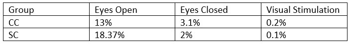
- What was the percentage of segments that needed to be rejected due to the 120μV criteria? This should be reported specifically for EO & EC and controls and patients.
The mean percentage of 1 second segments rejected for each resting state condition is below. Mean percentage of 6.25 long segments rejected in each group for the visual stimulation condition are also included, and will be added to the revised manuscript:
Author response table 3.
- The authors downsampled the data to 60Hz to "to match the stimulation rate". What is the intention of this? Because the subsequent spectral analyses are conflated by this choice (see Nyquist theorem).
This data were collected as part of a study designed to evoke alpha activity with visual white-noise, which ranged in luminance with equal power at all frequencies from 1-60 Hz, restricted by the refresh rate of the monitor on which stimuli were presented (Pant et al., 2023). This paradigm and method was developed by VanRullen and colleagues (Schwenk et al., 2020; Vanrullen & MacDonald, 2012), wherein the analysis requires the same sampling rate between the presented frequencies and the EEG data. The downsampling function used here automatically applies an anti-aliasing filter (EEGLAB 2019) .
- "Subsequently, baseline removal was conducted by subtracting the mean activity across the length of an epoch from every data point." The actual baseline time segment should be specified.
The time segment was the length of the epoch, that is, 1 second for the resting state conditions and 6.25 seconds for the visual stimulation conditions. This will be explicitly stated in the revised manuscript.
- "We excluded the alpha range (8-14 Hz) for this fit to avoid biasing the results due to documented differences in alpha activity between CC and SC individuals (Bottari et al., 2016; Ossandón et al., 2023; Pant et al., 2023)." This does not really make sense, as the FOOOF algorithm first fits the 1/f slope, for which the alpha activity is not relevant.
We did not use the FOOOF algorithm/toolbox in this manuscript. As stated in the methods, we used a 1/f fit to the 1-20 Hz spectrum in the log-log space, and subtracted this fit from the original spectrum to obtain the corrected spectrum. Given the pronounced difference in alpha power between groups (Bottari et al., 2016; Ossandón et al., 2023; Pant et al., 2023), we were concerned it might drive differences in the exponent values. Our analysis pipeline had been adapted from previous publications of our group and other labs (Ossandón et al., 2023; Voytek et al., 2015; Waschke et al., 2017).
We have conducted the analysis with and without the exclusion of the alpha range, as well as using the FOOOF toolbox both in the 1-20 Hz and 20-40 Hz ranges (Ossandón et al., 2023); The findings of a steeper slope in the 1-20 Hz range as well as lower alpha power in CC vs SC individuals remained stable. In Ossandón et al., the comparison between the piecewise fits and FOOOF fits led the authors to use the former as it outperformed the FOOOF algorithm for their data.
- The model fits of the 1/f fitting for EO, EC, and both participant groups should be reported.
In Figure 3 of the manuscript, we depicted the mean spectra and 1/f fits for each group. We will add the fit quality metrics and show individual subjects’ fits in the revised manuscript.
(3.6) Validity of GABA measurements and results:
- According the a newer study by the authors of the Gannet toolbox (https://analyticalsciencejournals.onlinelibrary.wiley.com/doi/abs/10.1002/nbm.5076), the reliability and reproducibility of the gamma-aminobutyric acid (GABA) measurement can vary significantly depending on acquisition and modeling parameter. Thus, did the author address these challenges?
We took care of data quality while acquiring MRS data by ensuring appropriate voxel placement and linewidth prior to scanning. Acquisition as well as modeling parameters were constant for both groups, so they cannot have driven group differences.
The linked article compares the reproducibility of GABA measurement using Osprey, which was released in 2020 and uses linear combination modeling to fit the peak as opposed to Gannet’s simple peak fitting (Hupfeld et al., 2024). The study finds better test-retest reliability for Osprey compared to Gannet’s method.
As the present work was conceptualized in 2018, we used Gannet 3.0, which was the state-of-the-art edited spectral analysis toolbox at the time, and still is widely used. In the revised manuscript, we will include a supplementary section reanalyzing the main findings with Osprey.
- Furthermore, the authors wrote: "We confirmed the within-subject stability of metabolite quantification by testing a subset of the sighted controls (n=6) 2-4 weeks apart. Looking at the supplementary Figure 5 (which would be rather plotted as ICC or Blant-Altman plots), the within-subject stability compared to between-subject variability seems not to be great. Furthermore, I don't think such a small sample size qualifies for a rigorous assessment of stability.
Indeed, we did not intend to provide a rigorous assessment of within-subject stability. Rather, we aimed to confirm that data quality/concentration ratios did not systematically differ between the same subjects tested longitudinally; driven, for example, by scanner heating or time of day. As with the phantom testing, we attempted to give readers an idea of the quality of the data, as they were collected from a primarily clinical rather than a research site.
In the revised manuscript we will remove the statement regarding stability, and add the Blant-Altman plot.
- "Why might an enhanced inhibitory drive, as indicated by the lower Glx/GABA ratio" Is this interpretation really warranted, as the results of the group differences in the Glx/GABA ratio seem to be rather driven by a decreased Glx concentration in CC rather than an increased GABA (see Figure 2).
We used the Glx/GABA+ ratio as a measure, rather than individual Glx or GABA+ concentration, which did not significantly differ between groups. As detailed in Response 2.2, we think this metric aligns better with an underlying E/I balance hypothesis and has been used in many previous studies (Gao et al., 2024; Liu et al., 2015; Narayan et al., 2022; Perica et al., 2022).
Our interpretation of an enhanced inhibitory drive additionally comes from the combination of aperiodic EEG (1-20 Hz) and MRS measures, which, when considered together, are consistent with a decreased E/I ratio.
In the revised manuscript, we will rephrase this sentence accordingly.
- Glx concentration predicted the aperiodic intercept in CC individuals' visual cortices during ambient and flickering visual stimulation. Why specifically investigate the Glx concentration, when the paper is about E/I ratio?
As stated in the methods, we exploratorily assessed the relationship between all MRS parameters (Glx, GABA+ and Glx/GABA+ ratio) with the aperiodic parameters (slope, offset), and corrected for multiple comparisons accordingly. We think this is a worthwhile analysis considering the rarity of the dataset/population (see 1.2, 1.6, 2.1 and reviewer 1’s comments about future hypotheses). We only report the Glx – aperiodic intercept correlation in the main manuscript as it survived correction for multiple comparisons.
(3.7) Interpretation of the correlation between MRS measurements and EEG aperiodic signal:
- The authors wrote: "The intercept of the aperiodic activity was highly correlated with the Glx concentration during rest with eyes open and during flickering stimulation (also see Supplementary Material S11). Based on the assumption that the aperiodic intercept reflects broadband firing (Manning et al., 2009; Winawer et al., 2013), this suggests that the Glx concentration might be related to broadband firing in CC individuals during active and passive visual stimulation." These results should not be interpreted (or with very caution) for several reasons (see also problem with influences on aperiodic intercept and small sample size). This is a result of the exploratory analyses of correlating every EEG parameter with every MRS parameter. This requires well-powered replication before any interpretation can be provided. Furthermore and importantly: why should this be specifically only in CC patients, but not in the SC control group?
We indicate clearly in all parts of the manuscript that these correlations are presented as exploratory. Further, we interpret the Glx-aperiodic offset correlation, and none of the others, as it survived the Bonferroni correction for multiple comparisons. We offer a hypothesis in the discussion section as to why such a correlation might exist in the CC but not the SC group (see response 2.2), and do not speculate further.
(3.8) Language and presentation:
- The manuscript requires language improvements and correction of numerous typos. Over-simplifications and unclear statements are present, which could mislead or confuse readers (see also interpretation of aperiodic signal).
In the revision, we will check that speculations are clearly marked and typos are removed.
- The authors state that "Together, the present results provide strong evidence for experience-dependent development of the E/I ratio in the human visual cortex, with consequences for behavior." The results of the study do not provide any strong evidence, because of the small sample size and exploratory analyses approach and not accounting for possible confounding factors.
We disagree with this statement and allude to convergent evidence of both MRS and neurophysiological measures. The latter link to corresponding results observed in a larger sample of CC individuals (Ossandón et al., 2023).
- "Our results imply a change in neurotransmitter concentrations as a consequence of *restoring* vision following congenital blindness." This is a speculative statement to infer a causal relationship on cross-sectional data.
As mentioned under 2.1, we conducted a cross-sectional study which might justify future longitudinal work. In order to advance science, new testable hypotheses were put forward at the end of a manuscript.
In the revised manuscript we will add “might imply” to better indicate the hypothetical character of this idea.
- In the limitation section, the authors wrote: "The sample size of the present study is relatively high for the rare population , but undoubtedly, overall, rather small." This sentence should be rewritten, as the study is plein underpowered. The further justification "We nevertheless think that our results are valid. Our findings neurochemically (Glx and GABA+ concentration), and anatomically (visual cortex) specific. The MRS parameters varied with parameters of the aperiodic EEG activity and visual acuity. The group differences for the EEG assessments corresponded to those of a larger sample of CC individuals (n=38) (Ossandón et al., 2023), and effects of chronological age were as expected from the literature." These statements do not provide any validation or justification of small samples. Furthermore, the current data set is a subset of an earlier published paper by the same authors "The EEG data sets reported here were part of data published earlier (Ossandón et al., 2023; Pant et al., 2023)." Thus, the statement "The group differences for the EEG assessments corresponded to those of a larger sample of CC individuals (n=38) " is a circular argument and should be avoided.
Our intention was not to justify having a small sample, but to justify why we think the results might be valid as they align with/replicate existing literature.
In the revised manuscript, we will add a figure showing that the EEG results of the 10 subjects considered here correspond to those of the 28 other subjects of Ossandon et al. We will adapt the text accordingly, clearly stating that the pattern of EEG results of the ten subjects reported here replicate those of the 28 additional subjects of Ossandon et al. (2023).
References
Barnes, S. J., Sammons, R. P., Jacobsen, R. I., Mackie, J., Keller, G. B., & Keck, T. (2015). Subnetwork-specific homeostatic plasticity in mouse visual cortex in vivo. Neuron, 86(5), 1290–1303. https://doi.org/10.1016/J.NEURON.2015.05.010
Bernabeu, A., Alfaro, A., García, M., & Fernández, E. (2009). Proton magnetic resonance spectroscopy (1H-MRS) reveals the presence of elevated myo-inositol in the occipital cortex of blind subjects. NeuroImage, 47(4), 1172–1176. https://doi.org/10.1016/j.neuroimage.2009.04.080
Bottari, D., Troje, N. F., Ley, P., Hense, M., Kekunnaya, R., & Röder, B. (2016). Sight restoration after congenital blindness does not reinstate alpha oscillatory activity in humans. Scientific Reports. https://doi.org/10.1038/srep24683
Colombo, M. A., Napolitani, M., Boly, M., Gosseries, O., Casarotto, S., Rosanova, M., Brichant, J. F., Boveroux, P., Rex, S., Laureys, S., Massimini, M., Chieregato, A., & Sarasso, S. (2019). The spectral exponent of the resting EEG indexes the presence of consciousness during unresponsiveness induced by propofol, xenon, and ketamine. NeuroImage, 189(September 2018), 631–644. https://doi.org/10.1016/j.neuroimage.2019.01.024
Consideration of Sample Size in Neuroscience Studies. (2020). Journal of Neuroscience, 40(21), 4076–4077. https://doi.org/10.1523/JNEUROSCI.0866-20.2020
Coullon, G. S. L., Emir, U. E., Fine, I., Watkins, K. E., & Bridge, H. (2015). Neurochemical changes in the pericalcarine cortex in congenital blindness attributable to bilateral anophthalmia. Journal of Neurophysiology. https://doi.org/10.1152/jn.00567.2015
Fang, Q., Li, Y. T., Peng, B., Li, Z., Zhang, L. I., & Tao, H. W. (2021). Balanced enhancements of synaptic excitation and inhibition underlie developmental maturation of receptive fields in the mouse visual cortex. Journal of Neuroscience, 41(49), 10065–10079. https://doi.org/10.1523/JNEUROSCI.0442-21.2021
Favaro, J., Colombo, M. A., Mikulan, E., Sartori, S., Nosadini, M., Pelizza, M. F., Rosanova, M., Sarasso, S., Massimini, M., & Toldo, I. (2023). The maturation of aperiodic EEG activity across development reveals a progressive differentiation of wakefulness from sleep. NeuroImage, 277. https://doi.org/10.1016/J.NEUROIMAGE.2023.120264
Gao, Y., Liu, Y., Zhao, S., Liu, Y., Zhang, C., Hui, S., Mikkelsen, M., Edden, R. A. E., Meng, X., Yu, B., & Xiao, L. (2024). MRS study on the correlation between frontal GABA+/Glx ratio and abnormal cognitive function in medication-naive patients with narcolepsy. Sleep Medicine, 119, 1–8. https://doi.org/10.1016/j.sleep.2024.04.004
Haider, B., Duque, A., Hasenstaub, A. R., & McCormick, D. A. (2006). Neocortical network activity in vivo is generated through a dynamic balance of excitation and inhibition. Journal of Neuroscience. https://doi.org/10.1523/JNEUROSCI.5297-05.2006
Hill, A. T., Clark, G. M., Bigelow, F. J., Lum, J. A. G., & Enticott, P. G. (2022). Periodic and aperiodic neural activity displays age-dependent changes across early-to-middle childhood. Developmental Cognitive Neuroscience, 54, 101076. https://doi.org/10.1016/J.DCN.2022.101076
Hupfeld, K. E., Zöllner, H. J., Hui, S. C. N., Song, Y., Murali-Manohar, S., Yedavalli, V., Oeltzschner, G., Prisciandaro, J. J., & Edden, R. A. E. (2024). Impact of acquisition and modeling parameters on the test–retest reproducibility of edited GABA+. NMR in Biomedicine, 37(4), e5076. https://doi.org/10.1002/nbm.5076
Hyvärinen, J., Carlson, S., & Hyvärinen, L. (1981). Early visual deprivation alters modality of neuronal responses in area 19 of monkey cortex. Neuroscience Letters, 26(3), 239–243. https://doi.org/10.1016/0304-3940(81)90139-7
Juchem, C., & Graaf, R. A. de. (2017). B0 magnetic field homogeneity and shimming for in vivo magnetic resonance spectroscopy. Analytical Biochemistry, 529, 17–29. https://doi.org/10.1016/j.ab.2016.06.003
Keck, T., Hübener, M., & Bonhoeffer, T. (2017). Interactions between synaptic homeostatic mechanisms: An attempt to reconcile BCM theory, synaptic scaling, and changing excitation/inhibition balance. Current Opinion in Neurobiology, 43, 87–93. https://doi.org/10.1016/J.CONB.2017.02.003
Kurcyus, K., Annac, E., Hanning, N. M., Harris, A. D., Oeltzschner, G., Edden, R., & Riedl, V. (2018). Opposite Dynamics of GABA and Glutamate Levels in the Occipital Cortex during Visual Processing. Journal of Neuroscience, 38(46), 9967–9976. https://doi.org/10.1523/JNEUROSCI.1214-18.2018
Liu, B., Wang, G., Gao, D., Gao, F., Zhao, B., Qiao, M., Yang, H., Yu, Y., Ren, F., Yang, P., Chen, W., & Rae, C. D. (2015). Alterations of GABA and glutamate-glutamine levels in premenstrual dysphoric disorder: A 3T proton magnetic resonance spectroscopy study. Psychiatry Research - Neuroimaging, 231(1), 64–70. https://doi.org/10.1016/J.PSCYCHRESNS.2014.10.020
Lunghi, C., Berchicci, M., Morrone, M. C., & Russo, F. D. (2015). Short‐term monocular deprivation alters early components of visual evoked potentials. The Journal of Physiology, 593(19), 4361. https://doi.org/10.1113/JP270950
Maier, S., Düppers, A. L., Runge, K., Dacko, M., Lange, T., Fangmeier, T., Riedel, A., Ebert, D., Endres, D., Domschke, K., Perlov, E., Nickel, K., & Tebartz van Elst, L. (2022). Increased prefrontal GABA concentrations in adults with autism spectrum disorders. Autism Research, 15(7), 1222–1236. https://doi.org/10.1002/aur.2740
Manning, J. R., Jacobs, J., Fried, I., & Kahana, M. J. (2009). Broadband shifts in local field potential power spectra are correlated with single-neuron spiking in humans. The Journal of Neuroscience : The Official Journal of the Society for Neuroscience, 29(43), 13613–13620. https://doi.org/10.1523/JNEUROSCI.2041-09.2009
McSweeney, M., Morales, S., Valadez, E. A., Buzzell, G. A., Yoder, L., Fifer, W. P., Pini, N., Shuffrey, L. C., Elliott, A. J., Isler, J. R., & Fox, N. A. (2023). Age-related trends in aperiodic EEG activity and alpha oscillations during early- to middle-childhood. NeuroImage, 269, 119925. https://doi.org/10.1016/j.neuroimage.2023.119925
Medel, V., Irani, M., Crossley, N., Ossandón, T., & Boncompte, G. (2023). Complexity and 1/f slope jointly reflect brain states. Scientific Reports, 13(1), 21700. https://doi.org/10.1038/s41598-023-47316-0
Medel, V., Irani, M., Ossandón, T., & Boncompte, G. (2020). Complexity and 1/f slope jointly reflect cortical states across different E/I balances. bioRxiv, 2020.09.15.298497. https://doi.org/10.1101/2020.09.15.298497
Molina, J. L., Voytek, B., Thomas, M. L., Joshi, Y. B., Bhakta, S. G., Talledo, J. A., Swerdlow, N. R., & Light, G. A. (2020). Memantine Effects on Electroencephalographic Measures of Putative Excitatory/Inhibitory Balance in Schizophrenia. Biological Psychiatry: Cognitive Neuroscience and Neuroimaging, 5(6), 562–568. https://doi.org/10.1016/j.bpsc.2020.02.004
Mukerji, A., Byrne, K. N., Yang, E., Levi, D. M., & Silver, M. A. (2022). Visual cortical γ−aminobutyric acid and perceptual suppression in amblyopia. Frontiers in Human Neuroscience, 16. https://doi.org/10.3389/fnhum.2022.949395
Muthukumaraswamy, S. D., & Liley, D. T. (2018). 1/F electrophysiological spectra in resting and drug-induced states can be explained by the dynamics of multiple oscillatory relaxation processes. NeuroImage, 179(November 2017), 582–595. https://doi.org/10.1016/j.neuroimage.2018.06.068
Narayan, G. A., Hill, K. R., Wengler, K., He, X., Wang, J., Yang, J., Parsey, R. V., & DeLorenzo, C. (2022). Does the change in glutamate to GABA ratio correlate with change in depression severity? A randomized, double-blind clinical trial. Molecular Psychiatry, 27(9), 3833—3841. https://doi.org/10.1038/s41380-022-01730-4
Nuijten, M. B., & Polanin, J. R. (2020). “statcheck”: Automatically detect statistical reporting inconsistencies to increase reproducibility of meta-analyses. Research Synthesis Methods, 11(5), 574–579. https://doi.org/10.1002/jrsm.1408
Ossandón, J. P., Stange, L., Gudi-Mindermann, H., Rimmele, J. M., Sourav, S., Bottari, D., Kekunnaya, R., & Röder, B. (2023). The development of oscillatory and aperiodic resting state activity is linked to a sensitive period in humans. NeuroImage, 275, 120171. https://doi.org/10.1016/J.NEUROIMAGE.2023.120171
Ostlund, B. D., Alperin, B. R., Drew, T., & Karalunas, S. L. (2021). Behavioral and cognitive correlates of the aperiodic (1/f-like) exponent of the EEG power spectrum in adolescents with and without ADHD. Developmental Cognitive Neuroscience, 48, 100931. https://doi.org/10.1016/j.dcn.2021.100931
Pant, R., Ossandón, J., Stange, L., Shareef, I., Kekunnaya, R., & Röder, B. (2023). Stimulus-evoked and resting-state alpha oscillations show a linked dependence on patterned visual experience for development. NeuroImage: Clinical, 103375. https://doi.org/10.1016/J.NICL.2023.103375
Perica, M. I., Calabro, F. J., Larsen, B., Foran, W., Yushmanov, V. E., Hetherington, H., Tervo-Clemmens, B., Moon, C.-H., & Luna, B. (2022). Development of frontal GABA and glutamate supports excitation/inhibition balance from adolescence into adulthood. Progress in Neurobiology, 219, 102370. https://doi.org/10.1016/j.pneurobio.2022.102370
Pitchaimuthu, K., Wu, Q. Z., Carter, O., Nguyen, B. N., Ahn, S., Egan, G. F., & McKendrick, A. M. (2017). Occipital GABA levels in older adults and their relationship to visual perceptual suppression. Scientific Reports, 7(1). https://doi.org/10.1038/S41598-017-14577-5
Rideaux, R., Ehrhardt, S. E., Wards, Y., Filmer, H. L., Jin, J., Deelchand, D. K., Marjańska, M., Mattingley, J. B., & Dux, P. E. (2022). On the relationship between GABA+ and glutamate across the brain. NeuroImage, 257, 119273. https://doi.org/10.1016/J.NEUROIMAGE.2022.119273
Schaworonkow, N., & Voytek, B. (2021). Longitudinal changes in aperiodic and periodic activity in electrophysiological recordings in the first seven months of life. Developmental Cognitive Neuroscience, 47. https://doi.org/10.1016/j.dcn.2020.100895
Schwenk, J. C. B., VanRullen, R., & Bremmer, F. (2020). Dynamics of Visual Perceptual Echoes Following Short-Term Visual Deprivation. Cerebral Cortex Communications, 1(1). https://doi.org/10.1093/TEXCOM/TGAA012
Sengpiel, F., Jirmann, K.-U., Vorobyov, V., & Eysel, U. T. (2006). Strabismic Suppression Is Mediated by Inhibitory Interactions in the Primary Visual Cortex. Cerebral Cortex, 16(12), 1750–1758. https://doi.org/10.1093/cercor/bhj110
Steel, A., Mikkelsen, M., Edden, R. A. E., & Robertson, C. E. (2020). Regional balance between glutamate+glutamine and GABA+ in the resting human brain. NeuroImage, 220. https://doi.org/10.1016/J.NEUROIMAGE.2020.117112
Takado, Y., Takuwa, H., Sampei, K., Urushihata, T., Takahashi, M., Shimojo, M., Uchida, S., Nitta, N., Shibata, S., Nagashima, K., Ochi, Y., Ono, M., Maeda, J., Tomita, Y., Sahara, N., Near, J., Aoki, I., Shibata, K., & Higuchi, M. (2022). MRS-measured glutamate versus GABA reflects excitatory versus inhibitory neural activities in awake mice. Journal of Cerebral Blood Flow & Metabolism, 42(1), 197. https://doi.org/10.1177/0271678X211045449
Takei, Y., Fujihara, K., Tagawa, M., Hironaga, N., Near, J., Kasagi, M., Takahashi, Y., Motegi, T., Suzuki, Y., Aoyama, Y., Sakurai, N., Yamaguchi, M., Tobimatsu, S., Ujita, K., Tsushima, Y., Narita, K., & Fukuda, M. (2016). The inhibition/excitation ratio related to task-induced oscillatory modulations during a working memory task: A multtimodal-imaging study using MEG and MRS. NeuroImage, 128, 302–315. https://doi.org/10.1016/J.NEUROIMAGE.2015.12.057
Tao, H. W., & Poo, M. M. (2005). Activity-dependent matching of excitatory and inhibitory inputs during refinement of visual receptive fields. Neuron, 45(6), 829–836. https://doi.org/10.1016/J.NEURON.2005.01.046
Vanrullen, R., & MacDonald, J. S. P. (2012). Perceptual echoes at 10 Hz in the human brain. Current Biology. https://doi.org/10.1016/j.cub.2012.03.050
Voytek, B., Kramer, M. A., Case, J., Lepage, K. Q., Tempesta, Z. R., Knight, R. T., & Gazzaley, A. (2015). Age-related changes in 1/f neural electrophysiological noise. Journal of Neuroscience, 35(38). https://doi.org/10.1523/JNEUROSCI.2332-14.2015
Vreeswijk, C. V., & Sompolinsky, H. (1996). Chaos in neuronal networks with balanced excitatory and inhibitory activity. Science, 274(5293), 1724–1726. https://doi.org/10.1126/SCIENCE.274.5293.1724
Waschke, L., Wöstmann, M., & Obleser, J. (2017). States and traits of neural irregularity in the age-varying human brain. Scientific Reports 2017 7:1, 7(1), 1–12. https://doi.org/10.1038/s41598-017-17766-4
Weaver, K. E., Richards, T. L., Saenz, M., Petropoulos, H., & Fine, I. (2013). Neurochemical changes within human early blind occipital cortex. Neuroscience. https://doi.org/10.1016/j.neuroscience.2013.08.004
Wu, Y. K., Miehl, C., & Gjorgjieva, J. (2022). Regulation of circuit organization and function through inhibitory synaptic plasticity. Trends in Neurosciences, 45(12), 884–898. https://doi.org/10.1016/J.TINS.2022.10.006