5,018 Matching Annotations
  1. Oct 2025
    1. Author response:

      Reviewer #1 (Public review):

      Summary:

      Loh and colleagues investigate valence encoding in the mesolimbic dopamine system. Using an elegant approach, they show that sucrose, which normally evokes strong dopamine neuron activity and release in the nucleus accumbens, is made aversive via conditioned taste aversion, the same sucrose stimulus later evokes much less dopamine neuron activity and release. Thus, dopamine activity can dynamically track the changing valence of an unconditioned stimulus. These results are important for helping clarify valence and value related questions that are the matter of ongoing debate regarding dopamine functions in the field.

      Strengths:

      This is an elegant way to ask this question, the within subject's design and the continuity of the stimulus is a strong way to remove a lot of the common confounds that make it difficult to interpret valence-related questions. I think these are valuable studies that help tie up questions in the field while also setting up a number of interesting future directions. There are number of control experiments and tweaks to the design that help eliminate a number of competing hypotheses regarding the results. The data are clearly presented and contextualized.

      Weaknesses for consideration:

      The focus on one relatively understudied region of the rat striatum for dopamine recordings could potentially limit generalization of the findings. While this can be determined in future studies, the implications should be further discussed in the current manuscript.

      We agree that the manuscript would benefit from providing a stronger rationale for our recording sites and acknowledging the potential for regional differences in dopamine signaling. We have made the following additions to the manuscript:

      Added to the Discussion: “Recordings were targeted to the lateral VTA and the corresponding approximate terminal site in the NAc lateral shell (Lammel et al., 2008). Subregional differences in dopamine activity likely contribute to mixed findings on dopamine and affect. For example, dopamine in the NAc lateral shell differentially encodes cues predictive of rewarding sucrose and aversive footshock, which is distinct from NAc medial shell dopamine responses (de Jong et al., 2019). Our findings are similar to prior work from our group targeting recordings to the NAc dorsomedial shell (Hsu et al., 2020; McCutcheon et al., 2012; Roitman et al., 2008): there, intraoral sucrose increased NAc dopamine release while the response in the same rats to quinine was significantly lower.”

      Reviewer #2 (Public review):

      Summary:

      Koh et al. report an interesting manuscript studying dopamine binding in the lateral accumbens shell of rats across the course of conditioned taste aversion. The question being asked here is how does the dopamine system respond to aversion? The authors take advantage of unique properties of taste aversion learning (notably, within-subjects remapping of valence to the same physical stimulus) to address this.

      They combine a well controlled behavioural design (including key, unpaired controls) with fibre photometry of dopamine binding via GrabDA and of dopamine neuron activity by gCaMP, careful analyses of behaviour (e.g., head movements; home cage ingestion), the authors show that, 1) conditioned taste aversion of sucrose suppresses the activity of VTA dopamine neurons and lateral shell dopamine binding to subsequent presentations of the sucrose tastant; 2) this pattern of activity was similar to the innately aversive tastant quinine; 3) dopamine responses were negatively correlated with behavioural (inferred taste reactivity) reactivity; and 4) dopamine responses tracked the contingency of between sucrose and illness because these responses recovered across extinction of the conditioned taste aversion.

      Strengths:

      There are important strengths here. The use of a well-controlled design, the measurement of both dopamine binding and VTA dopamine neuron activity, the inclusion of an extinction manipulation; and the thorough reporting of the data. I was not especially surprised by these results, but these data are a potentially important piece of the dopamine puzzle (e.g., as the authors note, salience-based argument struggles to explain these data).

      Weaknesses for consideration:

      (1) The focus here is on the lateral shell. This is a poorly investigated region in the context of the questions being asked here. Indeed, I suspect many readers might expect a focus on the medial shell. So, I think this focus is important. But, I think it does warrant greater attention in both the introduction and discussion. We do know from past work that there can be extensive compartmentalisation of dopamine responses to appetitive and aversive events and many of the inconsistent findings in the literature can be reconciled by careful examination of where dopamine is assessed. I do think readers would benefit from acknowledgement this - for example it is entirely reasonable to suppose that the findings here may be specific to the lateral shell.

      As with our response to Reviewer 1, we agree that we should provide further rationale for focusing our recordings on the lateral shell and acknowledge potential differences in dopamine dynamics across NAc subregions. In addition to the changes in the Discussion detailed in our response to Reviewer 1, we have made the following additions to the Introduction:

      Added to the Introduction: “NAc lateral shell dopamine differentially encodes cues predictive of rewarding (i.e., sipper spout with sucrose) and aversive stimuli (i.e., footshock), which is distinct from other subregions (de Jong et al., 2019). It is important to note that other regions of the NAc may serve as hedonic hotspots (e.g. dorsomedial shell; or may more closely align with the signaling of salience (e.g. ventromedial shell; (Yuan et al., 2021)).”

      (2) Relatedly, I think readers would benefit from an explicit rationale for studying the lateral shell as well as consideration of this in the discussion. We know that there are anatomical (PMID: 17574681), functional (PMID: 10357457), and cellular (PMID: 7906426) differences between the lateral shell and the rest of the ventral striatum. Critically, we know that profiles of dopamine binding during ingestive behaviours there can be highly dissimilar to the rest of ventral striatum (PMID: 32669355). I do think these points are worth considering.

      There are several reasons why dopamine dynamics were recorded in the NAc lateral shell:

      (1) Dopamine neurons in more medial aspects of the VTA preferentially target the NAc medial shell and core whereas dopamine neurons in the lateral VTA – our target for VTA DA recordings – project to the lateral shell of the NAc (Lammel et al., 2008). Thus, our goal was to sample NAc release dynamics in areas that receive projections from our cell body recording sites.

      (2) Cues predictive of reward availability (i.e., sipper spout with sucrose) and aversive stimuli (i.e., footshock) are differentially encoded by NAc lateral shell dopamine, which is distinct from NAc ventromedial shell dopamine responses (de Jong et al., 2019). These findings suggest a role for NAc lateral shell dopamine in the encoding of a stimulus’s valence, which made the subregion an area of interest for further examination.

      (3) With respect to the medial NAc shell specifically, extensive literature had already shown it to be a ‘hedonic hotspot’ (Morales and Berridge, 2020; Yuan et al., 2021) whereas the ventral portion is more mixed with respect to valence (Yuan et al., 2021). We had previously shown that intraoral infusions of primary taste stimuli of opposing valence (i.e., sucrose and quinine) evoke differential responses in dopamine release within the NAc dorsomedial shell (Roitman et al., 2008). We more recently replicated differential dopamine responses from dopamine cell bodies in the lateral VTA (Hsu et al., 2020) and thus endeavored to the possibility of changing dopamine responses in the lateral VTA to the same stimulus as its valence changes. As a result of these choices, measuring dopamine release in the lateral shell was a logical choice. The field would greatly benefit from continued future work surveying the entirety of the VTA DA projection terminus. 

      We have included these points of justification in the Introduction and Discussion sections.

      (3) I found the data to be very thoughtfully analysed. But in places I was somewhat unsure:

      (a) Please indicate clearly in the text when photometry data show averages across trials versus when they show averages across animals.

      We have now explicitly indicated in the figure legends of Figures 1, 3, 5, 7, and 8:

      (1) In heat maps, each row represents the averaged (across rats) response on that trial.

      (2) Traces below heat maps represent the response to infusion averaged first across trials for each rat and then across all rats.

      (3) Insets represent the average z-score across the infusion period averaged first across all trials for each rat and then across all rats.

      (b) I did struggle with the correlation analyses, for two reasons.

      (i) First, the key finding here is that the dopamine response to intraoral sucrose is suppressed by taste aversion. So, this will significantly restrict the range of dopamine transients, making interpretation of the correlations difficult.

      The overall hypothesis is that the dopamine response would correlate with the valence of a taste stimulus – even and especially when the stimulus remained constant but its valence changed. We inferred valence from the behavioral reactivity to the stimulus – reasoning that an appetitive taste will evoke minimal movement of the nose and paws (presumably because the animals are primarily engaging in small mouth movements associated with ingestion as shown by the seminal work of Grill and Norgren (1978) and the many studies published by the K.C. Berridge group) whereas an aversive taste will evoke significantly more movement as the rats engage in rejection responses (e.g. forelimb flails, chin rubs, etc.). When we conducted our regression analyses we endeavored to be as transparent as possible and labeled each symbol based on group (Unpaired vs Paired) and day (Conditioning vs Test). Both behavioral reactivity and dopamine responses change – but only for the Paired rats across days. In this sense, we believe the interpretation is clear. However, the Reviewer raises an important criticism that there would essentially be a floor effect with dopamine responses. We believe this is mitigated by data acquired across extinction and especially in Figure 9B. Here, the observations that dopamine responses fall to near zero but return to pre-conditioning levels in the Paired group with strong correlation between dopamine and behavioral reactivity throughout would hopefully partially allay the Reviewer’s concerns. See Part ii below for further support.

      (ii) Second, the authors report correlations by combining data across groups/conditions. I understand why the authors have done this, but it does risk obscuring differences between the groups. So, my question is: what happens to this trend when the correlations are computed separately for each group? I suspect other readers will share the same question. I think reporting these separate correlations would be very helpful for the field -

      regardless of the outcome.

      To address this concern, we performed separate regression analyses for Paired and Unpaired rats and provide the table below to detail results where data were combined across groups or separated. Expectedly, all analyses in Paired rats indicated a significant inverse relationship between dopamine and behavioral reactivity. Afterall, it is only in this group where behavioral reactivity to the taste stimulus changes as function of conditioning. Perhaps even more striking is that in almost all comparisons, even when restricting the regression analysis to Unpaired rats, we still observed a significant inverse relationship between dopamine and behavioral reactivity in most experiments. We have outlined the separated correlations below (asterisks denote slopes significantly different from 0; * p<0.05; ** p<0.01; *** p<0.005; **** p<0.001):

      Author response table 1.

      (4) Figure 1A is not as helpful as it might be. I do think readers would expect a more precise reporting of GCaMP expression in TH+ and TH- neurons. I also note that many of the nuances in terms of compartmentalisation of dopamine signalling discussed above apply to ventral tegmental area dopamine neurons (e.g. medial v lateral) and this is worth acknowledging when interpreting t

      Others have reported (Choi et al., 2020) and quantified (Hsu et al., 2020) GCaMP6f expression in TH+ neurons. While we didn’t report these quantifications, our observations were very much in line with previous quantifications from our laboratory (Hsu et al. 2020).

      We agree that we should elaborate on VTA subregional differences and have answered this response above (See responses to Reviewer 1 Weakness #1 and Reviewer 2 Weakness #2).

      Reviewer #3 (Public review):

      Summary:

      This study helps to clarify the mixed literature on dopamine responses to aversive stimuli. While it is well accepted that dopamine in the ventral striatum increases in response to various rewarding and appetitive stimuli, aversive stimuli have been shown to evoke phasic increases or decreasing depending on the exact aversive stimuli, behavioral paradigm, and/or dopamine recording method and location examined. Here the authors use a well-designed set of experiments to show differential responses to an appetitive primary reward (sucrose) that later becomes a conditioned aversive stimulus (sucrose previously paired with lithium chloride in a conditioned taste aversion paradigm). The results are interesting and add valuable data to the question of how the mesolimbic dopamine system encodes aversive stimuli, however, the conclusions are strongly stated given that the current data do not necessarily align with prior conflicting data in terms of recording location, and it is not clear exactly how to interpret the generally biphasic dopamine response to the CTA-sucrose which also evolves over exposures within a single session.

      Strengths:

      • The authors nicely demonstrate that their two aversive stimuli examined, quinine and sucrose following CTA, evoked aversive facial expressions and paw movements that differed from those following rewarding sucrose to support that the stimuli experienced by the rats differ in valence.

      • Examined dopamine responses to the exact same sensory stimuli conditioned to have opposing valences, avoiding standard confounds of appetitive and aversive stimuli being sensed by different sensory modalities (i.e., sweet taste vs. electric shock)

      • The authors examined multiple measurements of dopamine activity - cell body calcium (GCaMP6f) in midbrain and release in NAc (Grab-DA2h), which is useful as the prior mixed literature on aversive dopamine responses comes from a variety of recording methods.

      • Correlations between sucrose preference and dopamine signals demonstrate behavioral relevance of the differential dopamine signals.

      • The delayed testing experiment in Figure 7 nicely controls for the effect of time to demonstrate that the "rewarding" dopamine response to sucrose only recovers after multiple extinction sucrose exposures to extinguish the CTA.

      Weaknesses for consideration:

      (1) Regional differences in dopamine signaling to aversive stimuli are mentioned in the introduction and discussion. For instance, the idea that dopamine encodes salience is strongly argued against in the discussion, but the paper cited as arguing for that (Kutlu et al. 2021) is recording from the medial core in mice. Given other papers cited in the text about the regional differences in dopamine signaling in the NAc and from different populations of dopamine neurons in midbrain, it's important to mention this distinction wrt to salience signaling. Relatedly, the text says that the lateral NAc shell was targeted for accumbens recordings, but the histology figure looks like the majority of fibers were in the anterior lateral core of NAc. For the current paper to be a convincing last word on the issue, it would be extremely helpful to have similar recordings done in other parts of the NAc to do a more thorough comparison against other studies.

      As the Reviewer notes, NAc dopamine recordings were aimed at the lateral NAc shell. It is possible that some dopamine neurons lying within the anterior lateral core were recorded. Fiber photometry and the size of the fiber optics cannot definitively identify the precise location and number of dopamine neurons from which we recorded. Still, recording sites did not systematically differ between groups. Further, the within-subjects design helps to mitigate any potential biases for one subregion over another. The results presented in the manuscript strongly support a valence code. It is difficult to be the ‘last word’ on this topic and we suspect debate will continue. We used taste stimuli for appetitive and aversive stimuli – whereas many in the field will continue to use other noxious stimuli (e.g. foot shock) that likely recruit different circuits en route to the VTA. And there may very well be a different regional profile for dopamine signaling with different noxious stimuli. Moreover, we used intraoral infusion to avoid confounds of stimulus avoidance and competing motivations (e.g. food or fluid deprivation). We believe that this is one of the most important and unique features of our report. Recent work supports a role for phasic increases in dopamine in avoidance of noxious stimuli (Jung et al., 2024) and it will be critical for the field to reflect on the differences between avoidance and aversion. Moreover, in ongoing studies we aspire to fully survey dopamine signaling in conditioned taste aversion across the medial-lateral and dorsal-ventral axes of the VTA and NAc.

      (2) Dopamine release in the NAc never dips below baseline for the conditioned sucrose. Is it possible to really consider this as a signal for valence per se, as opposed to it being a weaker response relative to the original sucrose response?

      Indeed, NAc dopamine release to intraoral quinine nor aversive sucrose doesn’t dip below baseline but rather dopamine binding doesn’t change from pre-infusion baseline levels. It should be noted that VTA dopamine cell body activity does indeed dip below baseline in response to aversive sucrose. Moreover, using fast-scan cyclic voltammetry, we showed that dopamine release dips below baseline in the NAc dorsomedial shell in response to intraoral quinine (Roitman et al., 2008). The differences across recording sites may reflect regional differences but they may also reflect differences in recording approaches. GrabDA2h, used here, has relatively slow kinetics that may obscure dips below baseline (see response Weakness# 8 below).

      (3) Related to this, the main measure of the dopamine signal here, "mean z-score," obscures the temporal dynamics of the aversive dopamine response across a trial. This measure is used to claim that sucrose after CTA is "suppressing" dopamine neuron activity and release, which is true relative to the positive valence sucrose response. However, both GRAB-DA and cell-body GCaMP measurements show clear increases after onset of sucrose infusion before dipping back to baseline or slightly below in the average of all example experiments displayed. One could point to these data to argue either that aversive stimuli cause phasic increases in dopamine (due to the initial increase) or decreases (due to the delayed dip below baseline) depending on the measurement window. Some discussion of the dynamics of the response and how it relates to the prior literature would be useful.

      We have used mean z-score to do much of our quantitative analyses but the Reviewer raises the intriguing possibility that we are masking an initial increase in dopamine release and VTA DA activity evoked by aversive taste by doing so. We included the heat maps in the manuscript to be as transparent as possible about the time course of dopamine responses – both within a trial and across trials. The Reviewer’s point prompted us to reflect further on the heat maps and recognize that trials early in the session often showed a brief increase in dopamine for aversive sucrose but this response dissipated (NAc dopamine release) or flipped (VTA DA cell body activity) over trials. We now quantitatively characterize this feature by looking at the timecourse of dopamine responses in each third of the trials (1-10, 11-20, 21-30; see Author response images 1,2 and 3). As we infer the valence of the stimulus from nose and paw movements (behavioral reactivity), it is especially striking that we a similar timecourse for changes in behavior. Collectively, the data may reflect an updating process that is relatively slow and requires experience of the stimulus in a new (aversive) state – that is, a model-free process. While our experiments were not designed to test the updating of dopamine responses and discern their participation in model-based versus model-free learning processes – another debate in the dopamine field (Cone et al., 2016; Deserno et al., 2021)– the data reflect a model-free process. This is further supported in the experiment involving multiple conditioning sessions, where dopamine ‘dips’ are observed in trials 1-10 on Conditioning Day 3 and Extinction Day 1 when the new value of sucrose has been established. Finally, the relatively slow updating of the value of sucrose is reflected in older literature using a continuous intraoral infusion. Using this approach, rats began rejecting the saccharin infusion only after ~2min rather than immediately (Schafe et al., 1998; Schafe and Bernstein, 1996; Wilkins and Bernstein, 2006).   

      Author response image 1.

      Author response image 2.

      Author response image 3.

      (4) Would this delayed below-baseline dip be visible with a shorter infusion time?

      While our experiments did not explore this parameter, it would be interesting to parametrically vary infusion duration times and examine differences in dopamine responses. However, we believe the most parsimonious explanation is that the ‘dip’ in VTA cell body activity develops as a function of the slow updating of the value of sucrose reflective of a model-free process. We recognize that this is mere speculation.

      (5) Does the max of the increase or the dip of the decrease better correlate with the behavioral measures of aversion (orofacial, paw movements) or sucrose preference than "mean z-score" measure used here?

      It seems plausible that finding the most extreme value from baseline could better correlate to behavioral measures. Time courses to max increase and max decrease are different. Moreover, with appetitive sucrose, there are often multiple transients that occur throughout a single intraoral infusion. Coupled with a noisy time course for individual components of behavioral reactivity, we determined that averaging data across the whole infusion period (i.e. mean z-score) was the most objective way we could analyze the dopamine and behavioral responses to taste stimuli.

      (6) The authors argue strongly in the discussion against the idea that dopamine is encoding "salience." Could this initial peak (also seen in the first few trials of quinine delivery, fig 1c color plot) be a "salience" response?

      Our response above to the potential for ‘mixed’ dopamine responses to aversive sucrose led to additional analyses that support a slow updating of both behavior and dopamine to the new, aversive value of sucrose. Quinine is innately aversive and thus the Reviewer rightly points out that even here we observe an increase in dopamine release evoked by quinine on the first few trials (as observed in the heat map). We’d like to note, though, that the order of stimulus exposure was counterbalanced across rats. In those rats first receiving a sucrose session, quinine initially caused a modest increase in dopamine release during the first 10 trials (which is more pronounced in the first 2 trials). In the subsequent 2 blocks of 10 trials, no such increase was observed. Interestingly, in rats for which quinine was their first stimulus, we did not see an increase in dopamine release on the first few trials (see Author response image 4). We speculate that the initial sucrose session required the value of intraoral infusions to be updated when quinine was delivered to these rats and that, once more, the updating process may be slow and akin to a model-free process. This analysis, at present, is underpowered but will direct future attention in follow-up work.

      Author response image 4.

      (7) Related to this, the color plots showing individual trials show a reduction in the increases to positive valence sucrose across conditioning day trials and a flip from infusion-onset increase to delayed increases across test day trials. This evolution across days makes it appear that the last few conditioning day trials would be impossible to discriminate from the first few test day trials in the CTA-paired. Presumably, from strength of CTA as a paradigm, the sucrose is already aversive to the animals at the first trial of test day. Why do the authors think the response evolves across this session?

      As the Reviewer noted, Points 3-7 are related. We have speculated that the evolving dopamine response in Paired rats across test day trials reflects a model-free process. Importantly, as in the manuscript, our additional analyses once again show a tight relationship between behavioral reactivity and the dopamine response across the test session trials. It is important to note, though, that these experiments were not designed to test if responses reflect model-free or model-based processes.

      (8) Given that most of the work is using a conditioned aversive stimulus, the comparison to a primary aversive tastant quinine is useful. However, the authors saw basically no dopamine response to a primary aversive tastant quinine (measured only with GRAB-DA) and saw less noticeable decreases following CTA for NAc recordings with GRAB-DA2h than with cell body GCaMP. Given that they are using the high-affinity version of the GRAB sensor, this calls into question whether this is a true difference in release vs. soma activity or issue of high affinity release sensor making decreases in dopamine levels more difficult to observe.

      We share the same speculation as the Reviewer. Using fast-scan cyclic voltammetry, albeit measuring dopamine concentration in the dorsomedial shell, we observed a clear decrease from baseline with intraoral infusions of quinine (Roitman et al., 2008). Using fiber photometry here, the Reviewer and we note that GRAB_DA2h is a high-affinity (i.e., EC50: 7nM) dopamine sensor with relatively long off-kinetics (i.e., t1/2 decay time: 7300ms) (Labouesse et al., 2020). It may therefore be much more difficult to observe decreases (below baseline) using this sensor. The publication of new dopamine sensors - with lower affinity, faster kinetics, and greater dynamic range (Zhuo et al., 2024) – introduces opportunities for comparison and the greater potential for capturing decreases below baseline. Due to the poorer kinetics associated with GRAB_DA2h, we would not assert that direct comparisons between the GCaMP- and GRAB-based signals observed here represent true differences between somatic and terminal activity.

      References

      Choi JY, Jang HJ, Ornelas S, Fleming WT, Fürth D, Au J, Bandi A, Engel EA, Witten IB. 2020. A Comparison of Dopaminergic and Cholinergic Populations Reveals Unique Contributions of VTA Dopamine Neurons to Short-Term Memory. Cell Rep 33. doi:10.1016/j.celrep.2020.108492

      Cone JJ, Fortin SM, McHenry JA, Stuber GD, McCutcheon JE, Roitman MF. 2016. Physiological state gates acquisition and expression of mesolimbic reward prediction signals. Proc Natl Acad Sci U S A 113. doi:10.1073/pnas.1519643113

      de Jong JW, Afjei SA, Pollak Dorocic I, Peck JR, Liu C, Kim CK, Tian L, Deisseroth K, Lammel S. 2019. A Neural Circuit Mechanism for Encoding Aversive Stimuli in the Mesolimbic Dopamine System. Neuron 101. doi:10.1016/j.neuron.2018.11.005

      Deserno L, Moran R, Michely J, Lee Y, Dayan P, Dolan RJ. 2021. Dopamine enhances model-free credit assignment through boosting of retrospective model-based inference. Elife 10. doi:10.7554/eLife.67778

      Hsu TM, Bazzino P, Hurh SJ, Konanur VR, Roitman JD, Roitman MF. 2020. Thirst recruits phasic dopamine signaling through subfornical organ neurons. Proc Natl Acad Sci U S A 117:30744–30754. doi:10.1073/PNAS.2009233117/-/DCSUPPLEMENTAL

      Jung K, Krüssel S, Yoo S, An M, Burke B, Schappaugh N, Choi Y, Gu Z, Blackshaw S, Costa RM, Kwon HB. 2024. Dopamine-mediated formation of a memory module in the nucleus accumbens for goal-directed navigation. Nat Neurosci. doi:10.1038/s41593-024-01770-9

      Labouesse MA, Cola RB, Patriarchi T. 2020. GPCR-based dopamine sensors—A detailed guide to inform sensor choice for in vivo imaging. Int J Mol Sci. doi:10.3390/ijms21218048

      Lammel S, Hetzel A, Häckel O, Jones I, Liss B, Roeper J. 2008. Unique Properties of Mesoprefrontal Neurons within a Dual Mesocorticolimbic Dopamine System. Neuron 57. doi:10.1016/j.neuron.2008.01.022

      McCutcheon JE, Ebner SR, Loriaux AL, Roitman MF, Tobler PN. 2012. Encoding of aversion by dopamine and the nucleus accumbens. Front Neurosci 6. doi:10.3389/fnins.2012.00137

      Morales I, Berridge KC. 2020. ‘Liking’ and ‘wanting’ in eating and food reward: Brain mechanisms and clinical implications. Physiol Behav. doi:10.1016/j.physbeh.2020.113152

      Roitman MF, Wheeler RA, Wightman RM, Carelli RM. 2008. Real-time chemical responses in the nucleus accumbens differentiate rewarding and aversive stimuli. Nature Neuroscience 2008 11:12 11:1376–1377. doi:10.1038/nn.2219

      Schafe GE, Bernstein IL. 1996. Forebrain contribution to the induction of a brainstem correlate of conditioned taste aversion: I. The amygdala. Brain Res 741. doi:10.1016/S0006-8993(96)00906-7

      Schafe GE, Thiele TE, Bernstein IL. 1998. Conditioning method dramatically alters the role of amygdala in taste aversion learning. Learning and Memory 5. doi:10.1101/lm.5.6.481

      Wilkins EE, Bernstein IL. 2006. Conditioning method determines patterns of c-fos expression following novel taste-illness pairing. Behavioural Brain Research 169. doi:10.1016/j.bbr.2005.12.006

      Yuan L, Dou YN, Sun YG. 2021. Topography of reward and aversion encoding in the mesolimbic dopaminergic system. Journal of Neuroscience 39. doi:10.1523/JNEUROSCI.0271-19.2019

      Zhuo Y, Luo B, Yi X, Dong H, Miao X, Wan J, Williams JT, Campbell MG, Cai R, Qian T, Li F, Weber SJ, Wang L, Li B, Wei Y, Li G, Wang H, Zheng Y, Zhao Y, Wolf ME, Zhu Y, Watabe-Uchida M, Li Y. 2024. Improved green and red GRAB sensors for monitoring dopaminergic activity in vivo. Nat Methods 21. doi:10.1038/s41592-023-02100-w

    1. Author response:

      Responses to Editors:

      We appreciate Reviewer 1’s first concern regarding the difficulty of disentangling the contributions of tightly-coupled brain regions to the speech-gesture integration process—particularly due to the close temporal and spatial proximity of the stimulation windows and the potential for prolonged disruption. We would like to provide clarification and evidence supporting the validity of our methodology.

      Our previous study (Zhao et al., 2021, J. Neurosci) employed the same experimental protocol—using inhibitory double-pulse transcranial magnetic stimulation (TMS) over the inferior frontal gyrus (IFG) and posterior middle temporal gyrus (pMTG) in one of eight 40-ms time windows. The findings from that study demonstrated a time-window-selective disruption of the semantic congruency effect (i.e., reaction time costs driven by semantic conflict), with no significant modulation of the gender congruency effect (i.e., reaction time costs due to gender conflict). This result establishes that double-pulse TMS provides sufficient temporal precision to independently target the left IFG and pMTG within these 40-ms windows during gesture-speech integration. Importantly, by comparing the distinctively inhibited time windows for IFG and pMTG, we offered clear evidence of distinct engagement and temporal dynamics between these regions during different stages of gesture-speech semantic processing.

      Furthermore, we reviewed prior studies utilizing double-pulse TMS on structurally and functionally connected brain regions to explore neural contributions across timescales as brief as 3–60 ms. These studies, which encompass areas from the tongue and lip areas of the primary motor cortex (M1) to high-level semantic regions such as the pMTG and ATL (Author response table 1), consistently demonstrate the methodological rigor and precision of double-pulse TMS in disentangling the neural dynamics of different regions within these short temporal windows.

      Author response table 1.

      Double-pulse TMS studies on brain regions over 3-60 ms time interval

      Response to Reviewer #1:

      (1) For concern on the difficulty of disentangling the contributions of tightly-coupled brain regions to the speech-gesture integration process:

      We trust that the explanation provided above has clarified this issue.

      (2) For concern on the rationale for delivering HD-tDCS/TMS in set time windows for each region, as well as how these time windows were determined and how the current results compare to our previous studies from 2018 and 2023:

      The current study builds on a series of investigations that systematically examined the temporal and spatial dynamics of gesture-speech integration. In our earlier work (Zhao et al., 2018, J. Neurosci), we demonstrated that interrupting neural activity in the IFG or pMTG using TMS selectively disrupted the semantic congruency effect (reaction time costs due to semantic incongruence), without affecting the gender congruency effect (reaction time costs due to gender incongruence). These findings identified the IFG and pMTG as critical hubs for gesture-speech integration. This informed the brain regions selected for subsequent studies.

      In Zhao et al. (2021, J. Neurosci), we employed a double-pulse TMS protocol, delivering stimulation within one of eight 40-ms time windows, to further examine the temporal involvement of the IFG and pMTG. The results revealed time-window-selective disruptions of the semantic congruency effect, confirming the dynamic and temporally staged roles of these regions during gesture-speech integration.

      In Zhao et al. (2023, Frontiers in Psychology), we investigated the semantic predictive role of gestures relative to speech by comparing two experimental conditions: (1) gestures preceding speech by a fixed interval of 200 ms, and (2) gestures preceding speech at its semantic identification point. We observed time-window-selective disruptions of the semantic congruency effect in the IFG and pMTG only in the second condition, leading to the conclusion that gestures exert a semantic priming effect on co-occurring speech. These findings underscored the semantic advantage of gesture in facilitating speech integration, further refining our understanding of the temporal and functional interplay between these modalities.

      The design of the current study—including the choice of brain regions and time windows—was directly informed by these prior findings. Experiment 1 (HD-tDCS) targeted the entire gesture-speech integration process in the IFG and pMTG to assess whether neural activity in these regions, previously identified as integration hubs, is modulated by changes in informativeness from both modalities (i.e., entropy) and their interactions (mutual information, MI). The results revealed a gradual inhibition of neural activity in both areas as MI increased, evidenced by a negative correlation between MI and the tDCS inhibition effect in both regions. Building on this, Experiments 2 and 3 employed double-pulse TMS and event-related potentials (ERPs) to further assess whether the engaged neural activity was both time-sensitive and staged. These experiments also evaluated the contributions of various sources of information, revealing correlations between information-theoretic metrics and time-locked brain activity, providing insights into the ‘gradual’ nature of gesture-speech integration.

      We acknowledge that the rationale for the design of the current study was not fully articulated in the original manuscript. In the revised version, we will provide a more comprehensive and coherent explanation of the logic behind the three experiments, ensuring clear alignment with our previous findings.

      (3) For concern about the use of Pearson correlation and the normality of EEG data.

      We appreciate the reviewer’s thoughtful consideration. In Figure 5 of the manuscript, we have already included normal distribution curves that illustrate the relationships between the average ERP amplitudes within each ROI or elicited clusters and the three information models. Additionally, multiple comparisons were addressed using FDR correction, as outlined in the manuscript.

      To further clarify the data, we will calculate the Shapiro-Wilk test, a widely accepted method for assessing bivariate normality, for both the MI/entropy and averaged ERP data. The corresponding p-values will be provided in the following-up point-to-point responses.

      (4) For concern about the ROI selection, and the suggestion of using whole-brain electrodes to build models of different variables (MI/entropy) to predict neural responses:

      For the EEG data, we conducted both a traditional region-of-interest (ROI) analysis, with ROIs defined based on a well-established work (Habets et al., 2011), and a cluster-based permutation approach, which utilizes data-driven permutations to enhance robustness and address multiple comparisons. The latter method complements the hypothesis-driven ROI analysis by offering an exploratory, unbiased perspective. Notably, the results from both approaches were consistent, reinforcing the reliability of our findings.

      To make the methods more accessible to a broader audience, we will provide a clear description of the methods used and how they relate to each other in the revised manuscript.

      Reference:

      Habets, B., Kita, S., Shao, Z.S., Ozyurek, A., and Hagoort, P. (2011). The Role of Synchrony and Ambiguity in Speech-Gesture Integration during Comprehension. J Cognitive Neurosci 23, 1845-1854. 10.1162/jocn.2010.21462

      (5) For concern about the median split of the data:

      To identify ERP components or spatiotemporal clusters that demonstrated significant semantic differences, we split each model into higher and lower halves, focusing on indexing information changes reflected by entropy or mutual information (MI). To illustrate the gradual activation process, the identified components and clusters were further analyzed for correlations with each information matrix. Remarkably, consistent results were observed between the ERP components and clusters, providing robust evidence that semantic information conveyed through gestures and speech significantly influenced the amplitude of these components or clusters. Moreover, the semantic information was shown to be highly sensitive, varying in tandem with these amplitude changes.

      We acknowledge that the rationale behind this approach may not have been sufficiently clear in the initial manuscript. In our revision, we will ensure a more detailed and precise explanation to enhance the clarity and coherence of this logical framework.

      Response to Reviewer #2:

      We greatly appreciate Reviewer2 ’s concern regarding whether "mutual information" adequately captures the interplay between the meanings of speech and gesture. We would like to clarify that the materials used in the present study involved gestures performed without actual objects, paired with verbs that precisely describe the corresponding actions. For example, a hammering gesture was paired with the verb “hammer”, and a cutting gesture was paired with the verb “cut”. In this design, all gestures conveyed redundant meaning relative to the co-occurring speech, creating significant overlap between the information derived from speech alone and that from gesture alone.

      We understand the reviewer’s concern about cases where gestures and speech may provide complementary rather than redundant information. To address this, we have developed an alternative metric for quantifying information gains contributed by supplementary multisensory cues, which will be explored in a subsequent study. However, for the present study, we believe that the observed overlap in information serves as an indicator of the degree of multisensory convergence, a central focus of our investigation.

      Regarding the reviewer’s concern about how the neural processes of speech-gesture integration may change with variations in the relative timing between speech and gesture stimuli, we would like to highlight findings from our previous study (Zhao, 2023, Frontiers in Psychology). In that study, we explored the semantic predictive role of gestures relative to speech under two conditions: (1) gestures preceding speech by a fixed interval of 200 ms, and (2) gestures preceding speech of its semantic identification point. Interestingly, only in the second condition did we observe time-window-selective disruptions of the semantic congruency effect in the IFG and pMTG. This led us to conclude that gestures play a semantic priming role for co-occurring speech. Building on this, we designed the present study with gestures preceding speech of its semantic identification point to reflect this semantic priming relationship. Additionally, ongoing research is exploring gesture and speech interactions in natural conversational settings to investigate whether the neural processes identified here are consistent across varying contexts.

      To prevent any similar concerns from causing doubt among the audience and to ensure clarity regarding the follow-up study, we will provide a detailed discussion of the two issues in the revised manuscript.

      Response to Reviewer #3:

      The primary aim of this study is to investigate whether the degree of activity in the established integration hubs, IFG and pMTG, is influenced by the information provided by gesture-speech modalities and/or their interactions. While we provided evidence for the differential involvement of the IFG and pMTG by delineating their dynamic engagement across distinct time windows of gesture-speech integration and associating these patterns with unisensory information and their interaction, we acknowledge that the mechanisms underlying these dynamics remain open to interpretation. Specifically, whether the observed effects stem from difficulties in semantic control processes, as suggested by Reviewer 3, or from resolving information uncertainty, as quantified by entropy, falls outside the scope of the current study. Importantly, we view these two interpretations as complementary rather than mutually exclusive, as both may be contributing factors. Nonetheless, we agree that addressing this question is a compelling avenue for future research. In the revised manuscript, we will include an exploratory analysis to investigate whether the confounding difficulty, stemming from the number of lexical or semantic representations, is limited to high-entropy items. Additionally, we will address and discuss alternative interpretations.

      Regarding the concern of conceptual equivocation, we would like to emphasize that this study represents the first attempt to focus on the relationship between information quantity and neural engagement. In our initial presentation, we inadvertently conflated the commonly used term "graded hub," which refers to anatomical distribution, with its usage in the present context. We sincerely apologize for this oversight and are grateful for the reviewer’s careful critique. In the revised manuscript, we will clearly articulate the study’s objectives, clarify the representations of entropy and mutual information, and accurately describe their association with neural engagement.

      Reference

      Teige, C., Mollo, G., Millman, R., Savill, N., Smallwood, J., Cornelissen, P. L., & Jefferies, E. (2018). Dynamic semantic cognition: Characterising coherent and controlled conceptual retrieval through time using magnetoencephalography and chronometric transcranial magnetic stimulation. Cortex, 103, 329-349.

      Amemiya, T., Beck, B., Walsh, V., Gomi, H., & Haggard, P. (2017). Visual area V5/hMT+ contributes to perception of tactile motion direction: a TMS study. Scientific reports, 7(1), 40937.

      Muessgens, D., Thirugnanasambandam, N., Shitara, H., Popa, T., & Hallett, M. (2016). Dissociable roles of preSMA in motor sequence chunking and hand switching—a TMS study. Journal of Neurophysiology, 116(6), 2637-2646.

      Vernet, M., Brem, A. K., Farzan, F., & Pascual-Leone, A. (2015). Synchronous and opposite roles of the parietal and prefrontal cortices in bistable perception: a double-coil TMS–EEG study. Cortex, 64, 78-88.

      Pitcher, D. (2014). Facial expression recognition takes longer in the posterior superior temporal sulcus than in the occipital face area. Journal of Neuroscience, 34(27), 9173-9177.

      Bardi, L., Kanai, R., Mapelli, D., & Walsh, V. (2012). TMS of the FEF interferes with spatial conflict. Journal of cognitive neuroscience, 24(6), 1305-1313.

      D’Ausilio, A., Bufalari, I., Salmas, P., & Fadiga, L. (2012). The role of the motor system in discriminating normal and degraded speech sounds. Cortex, 48(7), 882-887.

      Pitcher, D., Duchaine, B., Walsh, V., & Kanwisher, N. (2010). TMS evidence for feedforward and feedback mechanisms of face and body perception. Journal of Vision, 10(7), 671-671.

      Gagnon, G., Blanchet, S., Grondin, S., & Schneider, C. (2010). Paired-pulse transcranial magnetic stimulation over the dorsolateral prefrontal cortex interferes with episodic encoding and retrieval for both verbal and non-verbal materials. Brain Research, 1344, 148-158.

      Kalla, R., Muggleton, N. G., Juan, C. H., Cowey, A., & Walsh, V. (2008). The timing of the involvement of the frontal eye fields and posterior parietal cortex in visual search. Neuroreport, 19(10), 1067-1071.

      Pitcher, D., Garrido, L., Walsh, V., & Duchaine, B. C. (2008). Transcranial magnetic stimulation disrupts the perception and embodiment of facial expressions. Journal of Neuroscience, 28(36), 8929-8933.

    1. Author Response

      We thank the reviewers and editorial team for the positive reaction to our paper and for the constructive recommendations and comments on our work. Here we provide a brief provisional response to key points that were identified. We will give a detailed point-by-point response with highlighted changes in our manuscript when we upload the revised version of our paper.

      Reviewer 1:

      Statistical evaluation of the null

      In Experiment 2, we inferred the existence of a null effect of image category on suppression depth based on frequentist statistics. At the reviewer’s suggestion we performed a statistical evaluation of the evidence in favour of the null effect using a Bayesian repeated measures ANOVA implemented in JASP. That analysis provides strong evidence for the null (BF01= 20.38) and will be included in the final version of the paper.

      Likelihood of exceptional cases

      We acknowledge that our selection of categories is only a sampling of possible categories to which our novel tCFS method can be applied for deriving suppression depth. Other possibilities that come to mind include objects that emerge from specific configurations of simple 'tokens' such as dots (such as actions defined by biological motion (Watson et al., 2004)) or different shaped tokens configured to generate pareidolia faces (Zhou et al., 2021). We will expand on the possibility of these exceptional cases impacting bCFS and reCFS thresholds in the discussion of our revised manuscript.

      Reviewer 2:

      In response to the claim “the paper overreaches by claiming breakthrough thresholds are insufficient for drawing certain conclusions about subconscious processing.”

      We agree that breakthrough thresholds can provide useful information to draw conclusions about unconscious processing – as our procedure is predicated on breakthrough thresholds. Our key point is that breakthrough provides only half of the needed information and will amend our manuscript accordingly. In so doing, we will also shift our focus toward the influence of semantics and low-level factors, including discussion of the possibility that suppression depth and bCFS thresholds could be driven by statistically orthogonal factors.

      Reviewer 3:

      On the appropriateness of log-transformed contrast

      Our motivation to quantify suppression depth after log-transform to decibel scale was two-fold. First, we recognised that the traditional use of a linear contrast ramp in bCFS is at odds with the well-characterised profile of contrast discrimination thresholds which obey a power law (Legge, 1981) and the observations that neural contrast response functions show the same compressive non-linearity in many different cortical processing areas (e.g.: V1, V2, V3, V4, MT, MST, FST, TEO. See Ekstrom et al., 2009). Increasing contrast in linear steps could thus lead to a rapid saturation of the response function, which may account for the overshoot that has been reported in many canonical bCFS studies. For example, in Jiang et al. (2007), target contrast reached 100% after 1 second, yet average suppression times for faces and inverted faces were 1.36 and 1.76 seconds respectively. As contrast response functions in visual neurons saturate at high contrast, the upper levels of a linear contrast ramp have less and less effect on the target's strength. This approach to response asymptote may have exaggerated small differences between stimulus conditions and may have inflated some previously reported differences. In sum, the use of a log-transformed contrast ramp allows finer increments in contrast to be explored before saturation, a simple manipulation which we hope will be adopted by our field.

      Second, by quantifying suppression depth as a decibel change, we enable the comparison of suppression depth between experiments and laboratories, which inevitably differ in presentation environments. As a comparison, a reaction-time for bCFS of 1.36 s cannot easily be compared without access to near-identical stimulation and testing environments. In addition, once ramp contrast is log-transformed it effectively linearises the neural contrast response function. This means that different studies that use different contrast levels for masker or target can be directly compared because a given suppression depth (for example, 15 dB) is the same proportionate difference between bCFS and reCFS regardless of the contrasts used in the particular study.

      We also acknowledge that different stimulus categories may engage neural and visual processing associated with different contrast gain values (e.g., magno- vs parvo-mediated processing). But the breaks and returns to suppression of a given stimulus category would be dependent on the same contrast gain function appropriate for that stimulus which thus permits their direct comparison. Indeed, this is why our novel approach offers a promising technique for comparing suppression depth associated with various stimulus categories (a point mentioned above). Viewed in this way, differences in actual durations of break times (such as we report in our paper) may tell us more about differences in gain control within neural mechanisms responsible for processing of those categories.

      Consider that preferential processing could shift both bCFS and reCFS thresholds together

      This is related to the point raised in the previous comment. A stimulus that is preferentially processed (such as a face) could have lower bCFS and reCFS thresholds than other stimuli such that it emerges into awareness at a lower contrast but also remains visible at lower contrasts. We plan to address this interpretation of our data in our revised discussion and highlight that this type of preferential processing could well occur, and yet could still produce the same uniform suppression depth.

      Can the effect of contrast ramp be explained by slower RTs?

      A 500 ms reaction time estimate would not account for the magnitude of the changes observed in Experiment 3. Suppression depths in our slow, medium, and fast contrast ramps were 9.64 dB, 14.64 dB and 18.97 dB, respectively (produced by step sizes of .035, .07 and .105 dB per video frame at 60 fps). At each rate, assuming a 500 ms reaction time for both thresholds (1 second total) would capture a change of 2.1 dB, 4.2 dB, 6.3 dB. This difference cannot account for the size of the effects observed between our different ramp speeds.

      Non-zero switch rate probability affecting ramping

      We agree that for a given ramp speed there is a variable probability of a switch in perceptual state for both bCFS and reCFS portions of the trial. To put it in other words, for a given ramp speed and a given observer the distribution of durations at which transitions occur will exhibit variance. We see that variance in our data (just as it’s present in conventional binocular rivalry duration histograms), as a non-zero probability of switches at very short durations (for example). One might surmise that slower ramp speeds would afford more opportunity for stochastic transitions to occur and that the measured suppression depths for slow ramps are underestimates of the suppression depth produced by contrast adaptation. Yet by the same token, the same underestimation would occur during fast ramp speeds, indicating that that difference may be even larger than we reported. In our revision we will spell this out in more detail, and indicate that a non-zero probability of switches at any time may lead to an underestimation of all recorded suppression depths.

      In our data, we believe the contribution of these stochastic switches are minimal. Our current Supplementary Figure 1(d) indicates that there is a non-zero probability of responses early in each ramp (e.g. durations < 2 seconds), yet these are a small proportion of all percept durations. This small proportion is clear in the empirical cumulative density function of percept durations, which we include in Author response image 1, and will address in our detailed response. Notably, during slow-ramp conditions, average percept durations actually increased, implying a resistance to any effect of early stochastic switching. We plan to expand on our analysis of these reaction-time differences in our revised manuscript.

      Author response image 1.

      The specificity of the DHO fit

      In our revised manuscript we will increase the justification for this model, and plan to include a comparison of model fits over time (as opposed to response number in the current manuscript).

      References

      Ekstrom, L. B., Roelfsema, P. R., Arsenault, J. T., Kolster, H., & Vanduffel, W. (2009). Modulation of the contrast response function by electrical microstimulation of the macaque frontal eye field. The Journal of Neuroscience: The Official Journal of the Society for Neuroscience, 29(34), 10683–10694.

      Jiang, Y., Costello, P., & He, S. (2007). Processing of invisible stimuli: advantage of upright faces and recognizable words in overcoming interocular suppression. Psychological Science, 18(4), 349–355.

      Legge, G. E. (1981). A power law for contrast discrimination. Vision Research, 21(4), 457–467.

      Watson, T. L., Pearson, J., & Clifford, C. W. G. (2004). Perceptual grouping of biological motion promotes binocular rivalry. Current Biology: CB, 14(18), 1670–1674.

      Zhou, L.-F., Wang, K., He, L., & Meng, M. (2021). Twofold advantages of face processing with or without visual awareness. Journal of Experimental Psychology. Human Perception and Performance, 47(6), 784–794.

    1. Author Response

      We thank the reviewers for their useful and constructive comments. In this provisional response, we will address a few of the major issues and plan to submit a detailed, point-by-point response along with the revised manuscript.

      1. Robustness of activated combination of neurons (the ‘activated ensemble’).

      The reviewers have asked for additional analyses and visualization of the group of neurons activated and a classification analysis to illustrate the point that the activated set of neurons would allow discrimination between different concentrations even after the spiking activity reduced significantly in the later trials. We relied on visualization using PCA (Manuscript Fig. 4) and quantification using correlation analysis (Manuscript Fig. 5a and Manuscript Supplementary Figure 2). But this point can be easily amplified further to support our conclusions and address a major concern raised by the reviewers.

      Visualization of neural responses across trials and odorants: As recommended, we followed the procedures used in Stopfer et al., 2003 (Fig. 6c) and Miura et al., 2012(Fig. 3C) to image neural responses across recorded PNs as a matrix (Author response image 1).

      Author response image 1.

      Author response image 1: Spike counts averaged over the entire 4s odor presentation window across all recorded neurons are shown as a function of trial number (columns). The sorting is same across different panels. Note that there are 80 neurons whose response was monitored for hexanol and octanol responses (Dataset 1; first row of panels), and 81 neurons whose response was monitored for isoamyl acetate and benzaldehyde (Dataset 2; second row of panels). As can be noted, across the 25 trials the pattern of activation remains consistent. Also, the activated combination of neurons varied robustly with odor identity and intensity.

      Classification analysis: To illustrate that there is enough information to recognize an odorant and discriminate between different intensities, we performed a leave-one-trial-out classification analysis. The left-out trial was assigned the class label of its nearest neighbor (using correlation distance metric). The results from this classification analysis are shown below in Author response image 2. As a control, we shuffled the odor class labels and repeated the leave-one-trial-out classification analysis.

      Author response image 2.

      Author response image 2: Results from classification analysis are shown for the two datasets: hexanol–octanol at different concentrations (dataset 1; 80 PNs), and isoamyl acetate and benzaldehyde (dataset 2; 81 PNs). We did a leave-onetrial-out validation. The true odor label is shown along the x-axis and the predicted odor label is shown along the yaxis. As can be noted, the class labels for every single trial were correctly predicted in both datasets. The result after class labels were shuffled is also shown for comparison. These results strongly support our conclusion that odor intensity information is preserved and odor concentration can be recognized independent of adaptation.

      Correlation with the first trial:

      We had shown the correlation across odorants and concentrations as a function of the trial (manuscript Figure 5A). To complement these analyses, here we focus on the correlations with the response evoked in the first trial of each odorant at high and low concentrations and plot this information as a function of trial number (Author response image 3, 4). As can be noted, the correlation across different trials of a given odorant at specific concentrations remains much higher than all other conditions.

      Author response image 3.

      Author response image 3: (top-left) Correlation between 80-dimensional neural responses (averaged over the entire 4s odor presentation window) with the first trial of hexanol at high intensity (hex-H; 1% v/v) is plotted as a function of trial number. (top-right) similar plots but correlation computed with neural responses evoked during the first trial of octanol at high intensity (oct-H; 1% v/v). (bottom-left) similar plots but correlation computed with neural responses evoked in the first trial of hexanol at low intensity (hex-L; 1% v/v). (bottom-right) similar plots but correlation computed with neural responses evoked in the first trial of octanol at low intensity (oct-L; 1% v/v).

      Author response image 4.

      Author response image 4: (top-left) Correlation between 81-dimensional neural responses (averaged over the entire 4s odor presentation window) with the first trial of isoamyl acetate at high intensity (iaa-H; 1% v/v) is plotted as a function of trial number. (top-right) similar plots but correlation computed with neural responses evoked in the first trial of benzaldehyde at a high intensity (bza-H; 1% v/v). (bottom-left) similar plots but correlation computed with neural responses evoked in the first trial of isoamyl acetate at low intensity (iaa-L; 1% v/v). (bottom-right) similar plots but correlation computed with neural responses evoked in the first trial of benzaldehyde at low intensity (bza-L; 1% v/v).

      Behavioral significance and dynamics: The reviewers had wondered about the relevance of the behavior to the organism. The maxillary palps are sensory organs close to the mouth parts that are used to grab food and help with the feeding process. In our previous studies, we had shown that these palpopening responses are innately triggered by many ‘appetitive odorants.’ However, the probability of palp opening varied across different odorants (Chandak and Raman, 2023). Some odorants evoked higher palp-opening responses and others reduced the probability of palp-opening response (below the median value across odorants). Since all other parameters (such as the clicking sound of valves, and mechanical cues due to airflow during odor presentation), are the same across these different odorants, these observed differences in palp-opening response probability are attributed to the identity of the odorants presented.

      Author response image 5.

      Author response image 5: Preference indices were calculated for all odors tested and are shown as a bar plot (n = 26 locusts). Blue bars indicate odors classified as appetitive, gray bars indicate neutral odors and red bars indicate unappetitive odors. Locusts with a significant deviation from the median response (one-sided binomial test, P < 0.1, were classified as either being appetitive or unappetitive; P < 0.1, P < 0.05, **P < 0.01). Error bars indicate s.e.m. [Replotted Fig 1.c from Chandak and Raman, 2023].

      We had also shown that we could train locusts to have stereo-typed palp-opening responses using the classical conditioning approach (odor – odor-conditioned stimulus and food reward – unconditioned stimulus; Video: https://static- content.springer.com/esm/art%3A10.1038%2Fncomms7953/MediaObjects/41467_2015_BFncomms7953 _MOESM483_ESM.mov; Saha et al., 2015). The dynamics of those conditioned palp-opening responses have been well characterized.

      We will use similar tracking procedures to monitor and quantify the dynamics of innate palp-opening responses as well. We will add supplementary videos to fully capture this behavior.

      Early vs. late neural responses:

      Since behavioral responses are more likely to start as soon as the odorant is presented, the reviewers wondered whether there are differences in the observed findings if we focus only on the early neural activity (as it might be more important to triggering behavior). Note that the median response time for conditioned palp-opening responses is less than 750 ms (Saha et al., 2015, Chandak and Raman, 2023). Hence, we divided the neural dataset and analyzed the neural response patterns during these early (0-750 ms after onset) and late (2-4 s after odor onset) time windows. In both these epochs, we found that the total spike counts across neurons reduced as a function of trial number or repetition and the combination of neuron activated remained robust (Author response images 6-11). Hence, we conclude that while the neural responses in different time windows would be important for shaping other parameters of behavioral response dynamics, the overall behavioral response probability that we used in our analysis had a similar relationship with early, late, or total neural activity during the entire odor presentation (i.e. time-window of the neural response did not matter for the analyses presented in the manuscript).

      Author response image 6.

      Author response image 6: Total spike counts reduced as a function of trial number. This reduction was observed for the total spike counts during the entire odor presentation window and during both the early (0-750 ms) and late (2-4 s) response time windows. Dataset 1: 80 PNs, hexanol, and octanol odorants.

      Author response image 7.

      Author response image 7: Total spike counts reduced as a function of trial number. This reduction was observed for the total spike counts during the entire odor presentation window and during both the early (0-750 ms) and late (2-4 s) response time windows. Dataset 2: 81 PNs, isoamyl acetate, and benzaldehyde odorants.

      Author response image 8.

      Author response image 8: Similar plots as in Figures 3 and 4 but analyzing 80-dimensional spike count vectors calculated using only the first 750 ms of odor-evoked response. Note that the correlation with the odor evoked response in the first trial remains high across trials. But between different odorants or different intensities of the same odorant, the response correlation drops significantly. Dataset 1: 80 PNs, hexanol, and octanol odorants.

      Author response image 9.

      Author response image 9: Similar plots as in Figures 3 and 4 but analyzing 80-dimensional spike count vectors calculated using only the last 2 seconds of odor-evoked response. Note that the correlation with the odor evoked response in the first trial remains high across trials. But between different odorants or different intensities of the same odorant, the response correlation drops significantly. Dataset 1: 80 PNs, hexanol, and octanol odorants.

      Author response image 10.

      Author response image 10: Similar plots as in Figures 3 and 4 but analyzing 80-dimensional spike count vectors calculated using only the first 750 ms of odor-evoked response. Note that the correlation with the odor evoked response in the first trial remains high across trials. But between different odorants or different intensities of the same odorant, the response correlation drops significantly. Dataset 2: 81 PNs, isoamyl acetate, and benzaldehyde odorants.

      Author response image 11.

      Author response image 11: Similar plots as in Figures 3 and 4 but analyzing 80-dimensional spike count vectors calculated using only the last 2 seconds of odor-evoked response. Note that the correlation with the odor evoked response in the first trial remains high across trials. But between different odorants or different intensities of the same odorant, the response correlation drops significantly. Dataset 2: 81 PNs, isoamyl acetate, and benzaldehyde odorants.

      Other Statistical Tests:

      The reviewers felt that in many analyses, we did not include error bars to indicate the sample size, SEM, or SD. We will fix this by adding the sample size information to each panel and as appropriate. However, we would also like to point out that many of the analyses are done in a trial-by-trial fashion (e.g. Manuscript Figures 3 – 6). For these analyses, it would not be possible to add SEM or SD. One condition (hex -H or iaa-H) was repeated in each dataset, and we have added them in the results shown in this response letter to demonstrate repeatability. We will strive our best to add these statistics as would be appropriate, but this cannot be done for the trial-by-trial analyses.

      References:

      Stopfer M, Jayaraman V, Laurent G. Intensity versus identity coding in an olfactory system. Neuron. 2003 Sep 11;39(6):991-1004. doi: 10.1016/j.neuron.2003.08.011. PMID: 12971898.

      Miura K, Mainen ZF, Uchida N. Odor representations in olfactory cortex: distributed rate coding and decorrelated population activity. Neuron. 2012 Jun 21;74(6):1087-98. doi: 10.1016/j.neuron.2012.04.021. PMID: 22726838; PMCID: PMC3383608.

      Chandak, R., Raman, B. Neural manifolds for odor-driven innate and acquired appetitive preferences. Nat Commun 14, 4719 (2023). https://doi.org/10.1038/s41467-023-40443-2

      Saha, D., Li, C., Peterson, S. et al. Behavioural correlates of combinatorial versus temporal features of odour codes. Nat Commun 6, 6953 (2015). https://doi.org/10.1038/ncomms7953

    1. Author response:

      Reviewer #1 (Public review):

      Wang et al., recorded concurrent EEG-fMRI in 107 participants during nocturnal NREM sleep to investigate brain activity and connectivity related to slow oscillations (SO), sleep spindles, and in particular their co-occurrence. The authors found SO-spindle coupling to be correlated with increased thalamic and hippocampal activity, and with increased functional connectivity from the hippocampus to the thalamus and from the thalamus to the neocortex, especially the medial prefrontal cortex (mPFC). They concluded the brain-wide activation pattern to resemble episodic memory processing, but to be dissociated from task-related processing and suggest that the thalamus plays a crucial role in coordinating the hippocampal-cortical dialogue during sleep.

      The paper offers an impressively large and highly valuable dataset that provides the opportunity for gaining important new insights into the network substrate involved in SOs, spindles, and their coupling. However, the paper does unfortunately not exploit the full potential of this dataset with the analyses currently provided, and the interpretation of the results is often not backed up by the results presented. I have the following specific comments.

      Thank you for your thoughtful and constructive feedback. We greatly appreciate your recognition of the strengths of our dataset and findings Below, we address your specific comments and provide responses to each point you raised to ensure our methods and results are as transparent and comprehensible as possible. We hope these revisions address your comments and further strengthen our manuscript. Thank you again for the constructive feedback.

      (1) The introduction is lacking sufficient review of the already existing literature on EEG-fMRI during sleep and the BOLD-correlates of slow oscillations and spindles in particular (Laufs et al., 2007; Schabus et al., 2007; Horovitz et al., 2008; Laufs, 2008; Czisch et al., 2009; Picchioni et al., 2010; Spoormaker et al., 2010; Caporro et al., 2011; Bergmann et al., 2012; Hale et al., 2016; Fogel et al., 2017; Moehlman et al., 2018; Ilhan-Bayrakci et al., 2022). The few studies mentioned are not discussed in terms of the methods used or insights gained.

      We acknowledge the need for a more comprehensive review of prior EEG-fMRI studies investigating BOLD correlates of slow oscillations and spindles. However, these articles are not all related to sleep SO or spindle. Articles (Hale et al., 2016; Horovitz et al., 2008; Laufs, 2008; Laufs, Walker, & Lund, 2007; Spoormaker et al., 2010) mainly focus on methodology for EEG-fMRI, sleep stages, or brain networks, which are not the focus of our study. Thank you again for your attention to the comprehensiveness of our literature review, and we will expand the introduction to include a more detailed discussion of the existing literature, ensuring that the contributions of previous EEG-fMRI sleep studies are adequately acknowledged.

      Introduction, Page 4 Lines 62-76

      “Investigating these sleep-related neural processes in humans is challenging because it requires tracking transient sleep rhythms while simultaneously assessing their widespread brain activation. Recent advances in simultaneous EEG-fMRI techniques provide a unique opportunity to explore these processes. EEG allows for precise event-based detection of neural signal, while fMRI provides insight into the broader spatial patterns of brain activation and functional connectivity (Horovitz et al., 2008; Huang et al., 2024; Laufs, 2008; Laufs, Walker, & Lund, 2007; Schabus et al., 2007; Spoormaker et al., 2010). Previous EEG-fMRI studies on sleep have focused on classifying sleep stages or examining the neural correlates of specific waves (Bergmann et al., 2012; Caporro et al., 2012; Czisch et al., 2009; Fogel et al., 2017; Hale et al., 2016; Ilhan-Bayrakcı et al., 2022; Moehlman et al., 2019; Picchioni et al., 2011). These studies have generally reported that slow oscillations are associated with widespread cortical and subcortical BOLD changes, whereas spindles elicit activation in the thalamus, as well as in several cortical and paralimbic regions. Although these findings provide valuable insights into the BOLD correlates of sleep rhythms, they often do not employ sophisticated temporal modeling (Huang et al., 2024), to capture the dynamic interactions between different oscillatory events, e.g., the coupling between SOs and spindles.”

      (2) The paper falls short in discussing the specific insights gained into the neurobiological substrate of the investigated slow oscillations, spindles, and their interactions. The validity of the inverse inference approach ("Open ended cognitive state decoding"), assuming certain cognitive functions to be related to these oscillations because of the brain regions/networks activated in temporal association with these events, is debatable at best. It is also unclear why eventually only episodic memory processing-like brain-wide activation is discussed further, despite the activity of 16 of 50 feature terms from the NeuroSynth v3 dataset were significant (episodic memory, declarative memory, working memory, task representation, language, learning, faces, visuospatial processing, category recognition, cognitive control, reading, cued attention, inhibition, and action).

      Thank you for pointing this out, particularly regarding the use of inverse inference approaches such as “open-ended cognitive state decoding.” Given the concerns about the indirectness of this approach, we decided to remove its related content and results from Figure 3 in the main text and include it in Supplementary Figure 7. We will refocus the main text on direct neurobiological insights gained from our EEG-fMRI analyses, particularly emphasizing the hippocampal-thalamocortical network dynamics underlying SO-spindle coupling, and we will acknowledge the exploratory nature of these findings and highlight their limitations.

      Discussion, Page 17-18 Lines 323-332

      “To explore functional relevance, we employed an open-ended cognitive state decoding approach using meta-analytic data (NeuroSynth: Yarkoni et al. (2011)). Although this method usefully generates hypotheses about potential cognitive processes, particularly in the absence of a pre- and post-sleep memory task, it is inherently indirect. Many cognitive terms showed significant associations (16 of 50), such as “episodic memory,” “declarative memory,” and “working memory.” We focused on episodic/declarative memory given the known link with hippocampal reactivation (Diekelmann & Born, 2010; Staresina et al., 2015; Staresina et al., 2023). Nonetheless, these inferences regarding memory reactivation should be interpreted cautiously without direct behavioral measures. Future research incorporating explicit tasks before and after sleep would more rigorously validate these potential functional claims.”

      (3) Hippocampal activation during SO-spindles is stated as a main hypothesis of the paper - for good reasons - however, other regions (e.g., several cortical as well as thalamic) would be equally expected given the known origin of both oscillations and the existing sleep-EEG-fMRI literature. However, this focus on the hippocampus contrasts with the focus on investigating the key role of the thalamus instead in the Results section.

      We appreciate your insight regarding the relative emphasis on hippocampal and thalamic activation in our study. We recognize that the manuscript may currently present an inconsistency between our initial hypothesis and the main focus of the results. To address this concern, we will ensure that our Introduction and Discussion section explicitly discusses both regions, highlighting the complementary roles of the hippocampus (memory processing and reactivation) and the thalamus (spindle generation and cortico-hippocampal coordination) in SO-spindle dynamics.

      Introduction, Page 5 Lines 87-103

      “To address this gap, our study investigates brain-wide activation and functional connectivity patterns associated with SO-spindle coupling, and employs a cognitive state decoding approach (Margulies et al., 2016; Yarkoni et al., 2011)—albeit indirectly—to infer potential cognitive functions. In the current study, we used simultaneous EEG-fMRI recordings during nocturnal naps (detailed sleep staging results are provided in the Methods and Table S1) in 107 participants. Although directly detecting hippocampal ripples using scalp EEG or fMRI is challenging, we expected that hippocampal activation in fMRI would coincide with SO-spindle coupling detected by EEG, given that SOs, spindles, and ripples frequently co-occur during NREM sleep. We also anticipated a critical role of the thalamus, particularly thalamic spindles, in coordinating hippocampal-cortical communication.

      We found significant coupling between SOs and spindles during NREM sleep (N2/3), with spindle peaks occurring slightly before the SO peak. This coupling was associated with increased activation in both the thalamus and hippocampus, with functional connectivity patterns suggesting thalamic coordination of hippocampal-cortical communication. These findings highlight the key role of the thalamus in coordinating hippocampal-cortical interactions during human sleep and provide new insights into the neural mechanisms underlying sleep-dependent brain communication. A deeper understanding of these mechanisms may contribute to future neuromodulation approaches aimed at enhancing sleep-dependent cognitive function and treating sleep-related disorders.”

      Discussion, Page 16-17 Lines 292-307

      “When modeling the timing of these sleep rhythms in the fMRI, we observed hippocampal activation selectively during SO-spindle events. This suggests the possibility of triple coupling (SOs–spindles–ripples), even though our scalp EEG was not sufficiently sensitive to detect hippocampal ripples—key markers of memory replay (Buzsáki, 2015). Recent iEEG evidence indicates that ripples often co-occur with both spindles (Ngo, Fell, & Staresina, 2020) and SOs (Staresina et al., 2015; Staresina et al., 2023). Therefore, the hippocampal involvement during SO-spindle events in our study may reflect memory replay from the hippocampus, propagated via thalamic spindles to distributed cortical regions.

      The thalamus, known to generate spindles (Halassa et al., 2011), plays a key role in producing and coordinating sleep rhythms (Coulon, Budde, & Pape, 2012; Crunelli et al., 2018), while the hippocampus is found essential for memory consolidation (Buzsáki, 2015; Diba & Buzsá ki, 2007; Singh, Norman, & Schapiro, 2022). The increased hippocampal and thalamic activity, along with strengthened connectivity between these regions and the mPFC during SO-spindle events, underscores a hippocampal-thalamic-neocortical information flow. This aligns with recent findings suggesting the thalamus orchestrates neocortical oscillations during sleep (Schreiner et al., 2022). The thalamus and hippocampus thus appear central to memory consolidation during sleep, guiding information transfer to the neocortex, e.g., mPFC.”

      (4) The study included an impressive number of 107 subjects. It is surprising though that only 31 subjects had to be excluded under these difficult recording conditions, especially since no adaptation night was performed. Since only subjects were excluded who slept less than 10 min (or had excessive head movements) there are likely several datasets included with comparably short durations and only a small number of SOs and spindles and even less combined SO-spindle events. A comprehensive table should be provided (supplement) including for each subject (included and excluded) the duration of included NREM sleep, number of SOs, spindles, and SO+spindle events. Also, some descriptive statistics (mean/SD/range) would be helpful.

      We appreciate your recognition of our sample size and the challenges associated with simultaneous EEG-fMRI sleep recordings. We acknowledge the importance of transparently reporting individual subject data, particularly regarding sleep duration and the number of detected SOs, spindles, and SO-spindle events. To address this, we will provide comprehensive tables in the supplementary materials, contains descriptive information about sleep-related characteristics (Table S1), as well as detailed information about sleep waves at each sleep stage for all 107 subjects(Table S2-S4), listing for each subject:(1)Different sleep stage duration; (2)Number of detected SOs; (3)Number of detected spindles; (4)Number of detected SO-spindle coupling events; (5)Density of detected SOs; (6)Density of detected spindles; (7)Density of detected SO-spindle coupling events.

      However, most of the excluded participants were unable to fall asleep or had too short a sleep duration, so they basically had no NREM sleep period, so it was impossible to count the NREM sleep duration, SO, spindle, and coupling numbers.

      Supplementary Materials, Page 42-54, Table S1-S4

      (Consider of the length, we do not list all the tables here. Please refer to the revised manuscript.)

      (5) Was the 20-channel head coil dedicated for EEG-fMRI measurements? How were the electrode cables guided through/out of the head coil? Usually, the 64-channel head coil is used for EEG-fMRI measurements in a Siemens PRISMA 3T scanner, which has a cable duct at the back that allows to guide the cables straight out of the head coil (to minimize MR-related artifacts). The choice for the 20-channel head coil should be motivated. Photos of the recording setup would also be helpful.

      Thank you for your comment regarding our choice of the 20-channel head coil for EEG-fMRI measurements. We acknowledge that the 64-channel head coil is commonly used in Siemens PRISMA 3T scanners; however, the 20-channel coil was selected due to specific practical and technical considerations in our study. In particular, the 20-channel head coil was compatible with our EEG system and ensured sufficient signal-to-noise ratio (SNR) for both EEG and fMRI acquisition. The EEG electrode cables were guided through the lateral and posterior openings of the head coil, secured with foam padding to reduce motion and minimize MR-related artifacts. Moreover, given the extended nature of nocturnal sleep recordings, the 20-channel coil allowed us to maintain participant comfort while still achieving high-quality simultaneous EEG-fMRI data.

      We have made this clearer in the revised manuscript.

      Methods, Page 20 Lines 385-392

      “All MRI data were acquired using a 20-channel head coil on a research-dedicated 3-Tesla Siemens Magnetom Prisma MRI scanner. Earplugs and cushions were provided for noise protection and head motion restriction. We chose the 20-channel head coil because it was compatible with our EEG system and ensured sufficient signal-to-noise ratio (SNR) for both EEG and fMRI acquisition. The EEG electrode cables were guided through the lateral and posterior openings of the head coil, secured with foam padding to reduce motion and minimize MR-related artifacts. Moreover, given the extended nature of nocturnal sleep recordings, the 20-channel coil helped maintain participant comfort while still achieving high-quality simultaneous EEG-fMRI data.”

      (6) Was the EEG sampling synchronized to the MR scanner (gradient system) clock (the 10 MHz signal; not referring to the volume TTL triggers here)? This is a requirement for stable gradient artifact shape over time and thus accurate gradient noise removal.

      Thank you for raising this important point. We confirm that the EEG sampling was synchronized to the MR scanner’s 10 MHz gradient system clock, ensuring a stable gradient artifact shape over time and enabling accurate artifact removal. This synchronization was achieved using the standard clock synchronization interface of the EEG amplifier, minimizing timing jitter and drift. As a result, the gradient artifact waveform remained stable across volumes, allowing for more effective artifact correction during preprocessing. We appreciate your attention to this critical aspect of EEG-fMRI data acquisition.

      We have made this clearer in the revised manuscript.

      Methods, Page 19-20 Lines 371-383

      “EEG was recorded simultaneously with fMRI data using an MR-compatible EEG amplifier system (BrainAmps MR-Plus, Brain Products, Germany), along with a specialized electrode cap. The recording was done using 64 channels in the international 10/20 system, with the reference channel positioned at FCz. In order to adhere to polysomnography (PSG) recording standards, six electrodes were removed from the EEG cap: one for electrocardiogram (ECG) recording, two for electrooculogram (EOG) recording, and three for electromyogram (EMG) recording. EEG data was recorded at a sample rate of 5000 Hz, the resistance of the reference and ground channels was kept below 10 kΩ, and the resistance of the other channels was kept below 20 kΩ. To synchronize the EEG and fMRI recordings, the BrainVision recording software (BrainProducts, Germany) was utilized to capture triggers from the MRI scanner. The EEG sampling was synchronized to the MR scanner’s 10 MHz gradient system clock, ensuring a stable gradient artifact shape over time and enabling accurate artifact removal. This was achieved via the standard clock synchronization interface of the EEG amplifier, minimizing timing jitter and drift.”

      (7) The TR is quite long and the voxel size is quite large in comparison to state-of-the-art EPI sequences. What was the rationale behind choosing a sequence with relatively low temporal and spatial resolution?

      We acknowledge that our chosen TR and voxel size are relatively long and large compared to state-of-the-art EPI sequences. This decision was made to optimize the signal-to-noise ratio (SNR) and reduce susceptibility-related distortions, which are particularly critical in EEG-fMRI sleep studies where head motion and physiological noise can be substantial. A longer TR allowed us to sample whole-brain activity with sufficient coverage, while a larger voxel size helped enhance BOLD sensitivity and minimize partial volume effects in deep brain structures such as the thalamus and hippocampus, which are key regions of interest in our study. We appreciate your concern and hope this clarification provides sufficient rationale for our sequence parameters.

      We have made this clearer in the revised manuscript.

      Methods, Page 20-21 Lines 398-408

      “Then, the “sleep” session began after the participants were instructed to try and fall asleep. For the functional scans, whole-brain images were acquired using k-space and steady-state T2*-weighted gradient echo-planar imaging (EPI) sequence that is sensitive to the BOLD contrast. This measures local magnetic changes caused by changes in blood oxygenation that accompany neural activity (sequence specification: 33 slices in interleaved ascending order, TR = 2000 ms, TE = 30 ms, voxel size = 3.5 × 3.5 × 4.2 mm<sup>3</sup>, FA = 90°, matrix = 64 × 64, gap = 0.7 mm). A relatively long TR and larger voxel size were chosen to optimize SNR and reduce susceptibility-related distortions, which are critical in EEG-fMRI sleep studies where head motion and physiological noise can be substantial. The longer TR allowed whole-brain coverage with sufficient temporal resolution, while the larger voxel size helped enhance BOLD sensitivity and minimize partial volume effects in deep brain structures (e.g., the thalamus and hippocampus), which are key regions of interest in this study.”

      (8) The anatomically defined ROIs are quite large. It should be elaborated on how this might reduce sensitivity to sleep rhythm-specific activity within sub-regions, especially for the thalamus, which has distinct nuclei involved in sleep functions.

      We appreciate your insight regarding the use of anatomically defined ROIs and their potential limitations in detecting sleep rhythm-specific activity within sub-regions, particularly in the thalamus. Given the distinct functional roles of thalamic nuclei in sleep processes, we acknowledge that using a single, large thalamic ROI may reduce sensitivity to localized activity patterns. To address this, we will discuss this limitation in the revised manuscript, acknowledging that our approach prioritizes whole-structure effects but may not fully capture nucleus-specific contributions.

      Discussion, Page 18 Lines 333-341

      “Despite providing new insights, our study has several limitations. First, our scalp EEG did not directly capture hippocampal ripples, preventing us from conclusively demonstrating triple coupling. Second, the combination of EEG-fMRI and the lack of a memory task limit our ability to parse fine-grained BOLD responses at the DOWN- vs. UP-states of SOs and link observed activations to behavioral outcomes. Third, the use of large anatomical ROIs may mask subregional contributions of specific thalamic nuclei or hippocampal subfields. Finally, without a memory task, we cannot establish a direct behavioral link between sleep-rhythm-locked activation and memory consolidation. Future studies combining techniques such as ultra-high-field fMRI or iEEG with cognitive tasks may refine our understanding of subregional network dynamics and functional significance during sleep.”

      (9) The study reports SO & spindle amplitudes & densities, as well as SO+spindle coupling, to be larger during N2/3 sleep compared to N1 and REM sleep, which is trivial but can be seen as a sanity check of the data. However, the amount of SOs and spindles reported for N1 and REM sleep is concerning, as per definition there should be hardly any (if SOs or spindles occur in N1 it becomes by definition N2, and the interval between spindles has to be considerably large in REM to still be scored as such). Thus, on the one hand, the report of these comparisons takes too much space in the main manuscript as it is trivial, but on the other hand, it raises concerns about the validity of the scoring.

      We appreciate your concern regarding the reported presence of SOs and spindles in N1 and REM sleep and the potential implications. Our detection method for detecting SO, spindle, and coupling were originally designed only for N2&N3 sleep data based on the characteristics of the data itself, and this method is widely recognized and used in the sleep research (Hahn et al., 2020; Helfrich et al., 2019; Helfrich et al., 2018; Ngo, Fell, & Staresina, 2020; Schreiner et al., 2022; Schreiner et al., 2021; Staresina et al., 2015; Staresina et al., 2023). While, because the detection methods for SO and spindle are based on percentiles, this method will always detect a certain number of events when used for other stages (N1 and REM) sleep data, but the differences between these events and those detected in stage N23 remain unclear. We will acknowledge the reasons for these results in the Methods section and emphasize that they are used only for sanity checks.

      Methods, Page 25 Lines 515-524

      “We note that the above methods for detecting SOs, spindles, and their couplings were originally developed for N2 and N3 sleep data, based on the specific characteristics of these stages. These methods are widely recognized in sleep research (Hahn et al., 2020; Helfrich et al., 2019; Helfrich et al., 2018; Ngo, Fell, & Staresina, 2020; Schreiner et al., 2022; Schreiner et al., 2021; Staresina et al., 2015; Staresina et al., 2023). However, because this percentile-based detection approach will inherently identify a certain number of events if applied to other stages (e.g., N1 and REM), the nature of these events in those stages remains unclear compared to N2/N3. We nevertheless identified and reported the detailed descriptive statistics of these sleep rhythms in all sleep stages, under the same operational definitions, both for completeness and as a sanity check. Within the same subject, there should be more SOs, spindles, and their couplings in N2/N3 than in N1 or REM (see also Figure S2-S4, Table S1-S4).”

      (10) Why was electrode F3 used to quantify the occurrence of SOs and spindles? Why not a midline frontal electrode like Fz (or a number of frontal electrodes for SOs) and Cz (or a number of centroparietal electrodes) for spindles to be closer to their maximum topography?

      We appreciate your suggestion regarding electrode selection for SO and spindle quantification. Our choice of F3 was primarily based on previous studies (Massimini et al., 2004; Molle et al., 2011), where bilateral frontal electrodes are commonly used for detecting SOs and spindles. Additionally, we considered the impact of MRI-related noise and, after a comprehensive evaluation, determined that F3 provided an optimal balance between signal quality and artifact minimization. We also acknowledge that alternative electrode choices, such as Fz for SOs and Cz for spindles, could provide additional insights into their topographical distributions.

      (11) Functional connectivity (hippocampus -> thalamus -> cortex (mPFC)) is reported to be increased during SO-spindle coupling and interpreted as evidence for coordination of hippocampo-neocortical communication likely by thalamic spindles. However, functional connectivity was only analysed during coupled SO+spindle events, not during isolated SOs or isolated spindles. Without the direct comparison of the connectivity patterns between these three events, it remains unclear whether this is specific for coupled SO+spindle events or rather associated with one or both of the other isolated events. The PPIs need to be conducted for those isolated events as well and compared statistically to the coupled events.

      We appreciate your critical perspective on our functional connectivity analysis and the interpretation of hippocampus-thalamus-cortex (mPFC) interactions during SO-spindle coupling. We acknowledge that, in the current analysis, functional connectivity was only examined during coupled SO-spindle events, without direct comparison to isolated SOs or isolated spindles. To address this concern, we have conducted PPI analyses for all three ROIs(Hippocampus, Thalamus, mPFC) and all three event types (SO-spindle couplings, isolated SOs, and isolated spindles). Our results indicate that neither isolated SOs nor isolated Spindles yielded significant connectivity changes in all three ROIs, as all failed to survive multiple comparison corrections. This suggests that the observed connectivity increase is specific to SO-spindle coupling, rather than being independently driven by either SOs or spindles alone.

      Results, Page 14 Lines 248-255

      “Crucially, the interaction between FC and SO-spindle coupling revealed that only the functional connectivity of hippocampus -> thalamus (ROI analysis, t<sub>(106)</sub> = 1.86, p = 0.0328) and thalamus -> mPFC (ROI analysis, t<sub>(106)</sub> = 1.98, p = 0.0251) significantly increased during SO-spindle coupling, with no significant changes in all other pathways (Fig. 4e). We also conducted PPI analyses for the other two events (SOs and spindles), and neither yielded significant connectivity changes in the three ROIs, as all failed to survive whole-brain FWE correction at the cluster level (p < 0.05). Together, these findings suggest that the thalamus, likely via spindles, coordinates hippocampal-cortical communication selectively during SO-spindle coupling, but not isolated SOs or spindle events alone.”

      (12) The limited temporal resolution of fMRI does indeed not allow for easily distinguishing between fMRI activation patterns related to SO-up- vs. SO-down-states. For this, one could try to extract the amplitudes of SO-up- and SO-down-states separately for each SO event and model them as two separate parametric modulators (with the risk of collinearity as they are likely correlated).

      We appreciate your insightful comment regarding the challenge of distinguishing fMRI activation patterns related to SO-up vs. SO-down states due to the limited temporal resolution of fMRI. While our current analysis does not differentiate between these two phases, we acknowledge that separately modeling SO-up and SO-down states using parametric modulators could provide a more refined understanding of their distinct neural correlates. However, as you notes, this approach carries the risk of collinearity, and there is indeed a high correlation between the two amplitudes across all subjects in our results (r=0.98). Future studies could explore more on leveraging high-temporal-resolution techniques. While implementing this in the current study is beyond our scope, we will acknowledge this limitation in the Discussion section.

      Discussion, Page 17 Lines 308-322

      “An intriguing aspect of our findings is the reduced DMN activity during SOs when modeled at the SO trough (DOWN-state). This reduced DMN activity may reflect large-scale neural inhibition characteristic of the SO trough. The DMN is typically active during internally oriented cognition (e.g., self-referential processing or mind-wandering) and is suppressed during external stimuli processing (Yeshurun, Nguyen, & Hasson, 2021). It is unlikely, however, that this suppression of DMN during SO events is related to a shift from internal cognition to external responses given it is during deep sleep time. Instead, it could be driven by the inherent rhythmic pattern of SOs, which makes it difficult to separate UP- from DOWN-states (the two temporal regressors were highly correlated, and similar brain activation during SOs events was obtained if modelled at the SO peak instead, Fig. S5). Since the amplitude at the SO trough is consistently larger than that at the SO peak, the neural activation we detected may primarily capture the large-scale inhibition from DOWN-state. Interestingly, no such DMN reduction was found during SO-spindle coupling, implying that coupling may involve distinct neural dynamics that partially re-engage DMN-related processes, possibly reflecting memory-related reactivation. Future research using high-temporal-resolution techniques like iEEG could clarify these possibilities.

      Discussion, Page 18 Lines 333-341

      “Despite providing new insights, our study has several limitations. First, our scalp EEG did not directly capture hippocampal ripples, preventing us from conclusively demonstrating triple coupling. Second, the combination of EEG-fMRI and the lack of a memory task limit our ability to parse fine-grained BOLD responses at the DOWN- vs. UP-states of SOs and link observed activations to behavioral outcomes. Third, the use of large anatomical ROIs may mask subregional contributions of specific thalamic nuclei or hippocampal subfields. Finally, without a memory task, we cannot establish a direct behavioral link between sleep-rhythm-locked activation and memory consolidation. Future studies combining techniques such as ultra-high-field fMRI or iEEG with cognitive tasks may refine our understanding of subregional network dynamics and functional significance during sleep.

      (13) L327: "It is likely that our findings of diminished DMN activity reflect brain activity during the SO DOWN-state, as this state consistently shows higher amplitude compared to the UP-state within subjects, which is why we modelled the SO trough as its onset in the fMRI analysis." This conclusion is not justified as the fact that SO down-states are larger in amplitude does not mean their impact on the BOLD response is larger.

      We appreciate your concern regarding our interpretation of diminished DMN activity reflecting the SO down-state. We acknowledge that the current expression is somewhat misleading, and our interpretation of it is: it could be driven by the inherent rhythmic pattern of SOs, which makes it difficult to separate UP- from DOWN-states (the two temporal regressors were highly correlated, and similar brain activation during SOs events was obtained if modelled at the SO peak instead). Since the amplitude at the SO trough is consistently larger than that at the SO peak, the neural activation we detected may primarily capture the large-scale inhibition from DOWN-state. And we will make this clear in the Discussion section.

      Discussion, Page 17 Lines 308-322

      “An intriguing aspect of our findings is the reduced DMN activity during SOs when modeled at the SO trough (DOWN-state). This reduced DMN activity may reflect large-scale neural inhibition characteristic of the SO trough. The DMN is typically active during internally oriented cognition (e.g., self-referential processing or mind-wandering) and is suppressed during external stimuli processing (Yeshurun, Nguyen, & Hasson, 2021). It is unlikely, however, that this suppression of DMN during SO events is related to a shift from internal cognition to external responses given it is during deep sleep time. Instead, it could be driven by the inherent rhythmic pattern of SOs, which makes it difficult to separate UP- from DOWN-states (the two temporal regressors were highly correlated, and similar brain activation during SOs events was obtained if modelled at the SO peak instead, Fig. S5). Since the amplitude at the SO trough is consistently larger than that at the SO peak, the neural activation we detected may primarily capture the large-scale inhibition from DOWN-state. Interestingly, no such DMN reduction was found during SO-spindle coupling, implying that coupling may involve distinct neural dynamics that partially re-engage DMN-related processes, possibly reflecting memory-related reactivation. Future research using high-temporal-resolution techniques like iEEG could clarify these possibilities.

      (14) Line 77: "In the current study, while directly capturing hippocampal ripples with scalp EEG or fMRI is difficult, we expect to observe hippocampal activation in fMRI whenever SOs-spindles coupling is detected by EEG, if SOs- spindles-ripples triple coupling occurs during human NREM sleep". Not all SO-spindle events are associated with ripples (Staresina et al., 2015), but hippocampal activation may also be expected based on the occurrence of spindles alone (Bergmann et al., 2012).

      We appreciate your clarification regarding the relationship between SO-spindle coupling and hippocampal ripples. We acknowledge that not all SO-spindle events are necessarily accompanied by ripples (Staresina et al., 2015). However, based on previous research, we found that hippocampal ripples are significantly more likely to occur during SO-spindle coupling events. This suggests that while ripple occurrence is not guaranteed, SO-spindle coupling creates a favorable network state for ripple generation and potential hippocampal activation. To ensure accuracy, we will revise the manuscript to delete this misleading sentence in the Introduction section and acknowledge in the Discussion that our results cannot conclusively directly observe the triple coupling of SO, spindle, and hippocampal ripples.

      Discussion, Page 18 Lines 333-341

      “Despite providing new insights, our study has several limitations. First, our scalp EEG did not directly capture hippocampal ripples, preventing us from conclusively demonstrating triple coupling. Second, the combination of EEG-fMRI and the lack of a memory task limit our ability to parse fine-grained BOLD responses at the DOWN- vs. UP-states of SOs and link observed activations to behavioral outcomes. Third, the use of large anatomical ROIs may mask subregional contributions of specific thalamic nuclei or hippocampal subfields. Finally, without a memory task, we cannot establish a direct behavioral link between sleep-rhythm-locked activation and memory consolidation. Future studies combining techniques such as ultra-high-field fMRI or iEEG with cognitive tasks may refine our understanding of subregional network dynamics and functional significance during sleep.”

      Reviewer #2 (Public review):

      In this study, Wang and colleagues aimed to explore brain-wide activation patterns associated with NREM sleep oscillations, including slow oscillations (SOs), spindles, and SO-spindle coupling events. Their findings reveal that SO-spindle events corresponded with increased activation in both the thalamus and hippocampus. Additionally, they observed that SO-spindle coupling was linked to heightened functional connectivity from the hippocampus to the thalamus, and from the thalamus to the medial prefrontal cortex-three key regions involved in memory consolidation and episodic memory processes.

      This study's findings are timely and highly relevant to the field. The authors' extensive data collection, involving 107 participants sleeping in an fMRI while undergoing simultaneous EEG recording, deserves special recognition. If shared, this unique dataset could lead to further valuable insights. While the conclusions of the data seem overall well supported by the data, some aspects with regard to the detection of sleep oscillations need clarification.

      The authors report that coupled SO-spindle events were most frequent during NREM sleep (2.46 [plus minus] 0.06 events/min), but they also observed a surprisingly high occurrence of these events during N1 and REM sleep (2.23 [plus minus] 0.09 and 2.32 [plus minus] 0.09 events/min, respectively), where SO-spindle coupling would not typically be expected. Combined with the relatively modest SO amplitudes reported (~25 µV, whereas >75 µV would be expected when using mastoids as reference electrodes), this raises the possibility that the parameters used for event detection may not have been conservative enough - or that sleep staging was inaccurately performed. This issue could present a significant challenge, as the fMRI findings are largely dependent on the reliability of these detected events.

      Thank you very much for your thorough and encouraging review. We appreciate your recognition of the significance and relevance of our study and dataset, particularly in highlighting how simultaneous EEG-fMRI recordings can provide complementary insights into the temporal dynamics of neural oscillations and their associated spatial activation patterns during sleep. In the sections that follow, we address each of your comments in detail. We have revised the text and conducted additional analyses wherever possible to strengthen our argument, clarify our methodological choices. We believe these revisions improve the clarity and rigor of our work, and we thank you for helping us refine it.

      We appreciate your insightful comments regarding the detection of sleep oscillations. Our methods for detecting SOs, spindles, and their couplings were originally developed for N2 and N3 sleep data, based on the specific characteristics of these stages. These methods are widely recognized in sleep research (Hahn et al., 2020; Helfrich et al., 2019; Helfrich et al., 2018; Ngo, Fell, & Staresina, 2020; Schreiner et al., 2022; Schreiner et al., 2021; Staresina et al., 2015; Staresina et al., 2023). However, because this percentile-based detection approach will inherently identify a certain number of events if applied to other stages (e.g., N1 and REM), the nature of these events in those stages remains unclear compared to N2/N3. We nevertheless identified and reported the detailed descriptive statistics of these sleep rhythms in all sleep stages, under the same operational definitions, both for completeness and as a sanity check. Within the same subject, there should be more SOs, spindles, and their couplings in N2/N3 than in N1 or REM. We will acknowledge the reasons for these results in the Methods section and emphasize that they are used only for sanity checks.

      Regarding the reported SO amplitudes (~25 µV), during preprocessing, we applied the Signal Space Projection (SSP) method to more effectively remove MRI gradient artifacts and cardiac pulse noise. While this approach enhances data quality, it also reduces overall signal power, leading to systematically lower reported amplitudes. Despite this, our SO detection in NREM sleep (especially N2/N3) remain physiologically meaningful and are consistent with previous fMRI studies using similar artifact removal techniques. We appreciate your careful evaluation and valuable suggestions.

      In addition, we will provide comprehensive tables in the supplementary materials, contains descriptive information about sleep-related characteristics (Table S1), as well as detailed information about sleep waves at each sleep stage for all 107 subjects(Table S2-S4), listing for each subject:(1)Different sleep stage duration; (2)Number of detected SOs; (3)Number of detected spindles; (4)Number of detected SO-spindle coupling events; (2)Density of detected SOs; (3)Density of detected spindles; (4)Density of detected SO-spindle coupling events.

      Methods, Page 25 Lines 515-524

      “We note that the above methods for detecting SOs, spindles, and their couplings were originally developed for N2 and N3 sleep data, based on the specific characteristics of these stages. These methods are widely recognized in sleep research (Hahn et al., 2020; Helfrich et al., 2019; Helfrich et al., 2018; Ngo, Fell, & Staresina, 2020; Schreiner et al., 2022; Schreiner et al., 2021; Staresina et al., 2015; Staresina et al., 2023). However, because this percentile-based detection approach will inherently identify a certain number of events if applied to other stages (e.g., N1 and REM), the nature of these events in those stages remains unclear compared to N2/N3. We nevertheless identified and reported the detailed descriptive statistics of these sleep rhythms in all sleep stages, under the same operational definitions, both for completeness and as a sanity check. Within the same subject, there should be more SOs, spindles, and their couplings in N2/N3 than in N1 or REM (see also Figure S2-S4, Table S1-S4).”

      Supplementary Materials, Page 42-54, Table S1-S4

      (Consider of the length, we do not list all the tables here. Please refer to the revised manuscript.)

      Reviewer #3 (Public review):

      Summary:

      Wang et al., examined the brain activity patterns during sleep, especially when locked to those canonical sleep rhythms such as SO, spindle, and their coupling. Analyzing data from a large sample, the authors found significant coupling between spindles and SOs, particularly during the upstate of the SO. Moreover, the authors examined the patterns of whole-brain activity locked to these sleep rhythms. To understand the functional significance of these brain activities, the authors further conducted open-ended cognitive state decoding and found a variety of cognitive processing may be involved during SO-spindle coupling and during other sleep events. The authors next investigated the functional connectivity analyses and found enhanced connectivity between the hippocampus, the thalamus, and the medial PFC. These results reinforced the theoretical model of sleep-dependent memory consolidation, such that SO-spindle coupling is conducive to systems-level memory reactivation and consolidation.

      Strengths:

      There are obvious strengths in this work, including the large sample size, state-of-the-art neuroimaging and neural oscillation analyses, and the richness of results.

      Weaknesses:

      Despite these strengths and the insights gained, there are weaknesses in the design, the analyses, and inferences.

      Thank you for your detailed and thoughtful review of our manuscript. We are delighted that you recognize our advanced analysis methods and rich results of neuroimaging and neural oscillations as well as the large sample size data. In the following sections, we provide detailed responses to each of your comments. And we have revised the text and conducted additional analyses to strengthen our arguments and clarify our methodological choices. We believe these revisions enhance the clarity and rigor of our work, and we sincerely appreciate your thoughtful feedback in helping us refine the manuscript.

      (1) A repeating statement in the manuscript is that brain activity could indicate memory reactivation and thus consolidation. This is indeed a highly relevant question that could be informed by the current data/results. However, an inherent weakness of the design is that there is no memory task before and after sleep. Thus, it is difficult (if not impossible) to make a strong argument linking SO/spindle/coupling-locked brain activity with memory reactivation or consolidation.

      We appreciate your suggestion regarding the lack of a pre- and post-sleep memory task in our study design. We acknowledge that, in the absence of behavioral measures, it is hard to directly link SO-spindle coupling to memory consolidation in an outcome-driven manner. Our interpretation is instead based on the well-established role of these oscillations in memory processes, as demonstrated in previous studies. We sincerely appreciate this feedback and will adjust our Discussion accordingly to reflect a more precise interpretation of our findings.

      Discussion, Page 18 Lines 333-341

      “Despite providing new insights, our study has several limitations. First, our scalp EEG did not directly capture hippocampal ripples, preventing us from conclusively demonstrating triple coupling. Second, the combination of EEG-fMRI and the lack of a memory task limit our ability to parse fine-grained BOLD responses at the DOWN- vs. UP-states of SOs and link observed activations to behavioral outcomes. Third, the use of large anatomical ROIs may mask subregional contributions of specific thalamic nuclei or hippocampal subfields. Finally, without a memory task, we cannot establish a direct behavioral link between sleep-rhythm-locked activation and memory consolidation. Future studies combining techniques such as ultra-high-field fMRI or iEEG with cognitive tasks may refine our understanding of subregional network dynamics and functional significance during sleep.”

      (2) Relatedly, to understand the functional implications of the sleep rhythm-locked brain activity, the authors employed the "open-ended cognitive state decoding" method. While this method is interesting, it is rather indirect given that there were no behavioral indices in the manuscript. Thus, discussions based on these analyses are speculative at best. Please either tone down the language or find additional evidence to support these claims.

      Moreover, the results from this method are difficult to understand. Figure 3e showed that for all three types of sleep events (SO, spindle, SO-spindle), the same mental states (e.g., working memory, episodic memory, declarative memory) showed opposite directions of activation (left and right panels showed negative and positive activation, respectively). How to interpret these conflicting results? This ambiguity is also reflected by the term used: declarative memory and episodic memories are both indexed in the results. Yet these two processes can be largely overlapped. So which specific memory processes do these brain activity patterns reflect? The Discussion shall discuss these results and the limitations of this method.

      We appreciate your critical assessment of the open-ended cognitive state decoding method and its interpretational challenges. Given the concerns about the indirectness of this approach, we decided to remove its related content and results from Figure 3 in the main text and include it in Supplementary Figure 7.

      Due to the complexity of memory-related processes, we acknowledge that distinguishing between episodic and declarative memory based solely on this approach is not straightforward. We will revise the Supplementary Materials to explicitly discuss these limitations and clarify that our findings do not isolate specific cognitive processes but rather suggest general associations with memory-related networks.

      Discussion, Page 17-18 Lines 323-332

      “To explore functional relevance, we employed an open-ended cognitive state decoding approach using meta-analytic data (NeuroSynth: Yarkoni et al. (2011)). Although this method usefully generates hypotheses about potential cognitive processes, particularly in the absence of a pre- and post-sleep memory task, it is inherently indirect. Many cognitive terms showed significant associations (16 of 50), such as “episodic memory,” “declarative memory,” and “working memory.” We focused on episodic/declarative memory given the known link with hippocampal reactivation (Diekelmann & Born, 2010; Staresina et al., 2015; Staresina et al., 2023). Nonetheless, these inferences regarding memory reactivation should be interpreted cautiously without direct behavioral measures. Future research incorporating explicit tasks before and after sleep would more rigorously validate these potenial functional claims.”

      (3) The coupling strength is somehow inconsistent with prior results (Hahn et al., 2020, eLife, Helfrich et al., 2018, Neuron). Specifically, Helfrich et al. showed that among young adults, the spindle is coupled to the peak of the SO. Here, the authors reported that the spindles were coupled to down-to-up transitions of SO and before the SO peak. It is possible that participants' age may influence the coupling (see Helfrich et al., 2018). Please discuss the findings in the context of previous research on SO-spindle coupling.

      We appreciate your concern regarding the temporal characteristics of SO-spindle coupling. We acknowledge that the SO-spindle coupling phase results in our study are not identical to those reported by Hahn et al. (2020); Helfrich et al. (2018). However, these differences may arise due to slight variations in event detection parameters, which can influence the precise phase estimation of coupling. Notably, Hahn et al. (2020) also reported slight discrepancies in their group-level coupling phase results, highlighting that methodological differences can contribute to variability across studies. Furthermore, our findings are consistent with those of Schreiner et al. (2021), further supporting the robustness of our observations.

      That said, we acknowledge that our original description of SO-spindle coupling as occurring at the "transition from the lower state to the upper state" was not entirely precise. The -π/2 phase represents the true transition point, while our observed coupling phase is actually closer to the SO peak rather than strictly at the transition. We will revise this statement in the manuscript to ensure clarity and accuracy in describing the coupling phase.

      Discussion, Page 16 Lines 283-291

      “Our data provide insights into the neurobiological underpinnings of these sleep rhythms. SOs, originating mainly in neocortical areas such as the mPFC, alternate between DOWN- and UP-states. The thalamus generates sleep spindles, which in turn couple with SOs. Our finding that spindle peaks consistently occurred slightly before the UP-state peak of SOs (in 83 out of 107 participants), concurs with prior studies, including Schreiner et al. (2021). Yet it differs from some results suggesting spindles might peak right at the SO UP-state (Hahn et al., 2020; Helfrich et al., 2018). Such discrepancies could arise from differences in detection algorithms, participant age (Helfrich et al., 2018), or subtle variations in cortical-thalamic timing. Nonetheless, these results underscore the importance of coordinated SO-spindle interplay in supporting sleep-dependent processes.”

      (4) The discussion is rather superficial with only two pages, without delving into many important arguments regarding the possible functional significance of these results. For example, the author wrote, "This internal processing contrasts with the brain patterns associated with external tasks, such as working memory." Without any references to working memory, and without delineating why WM is considered as an external task even working memory operations can be internal. Similarly, for the interesting results on SO and reduced DMN activity, the authors wrote "The DMN is typically active during wakeful rest and is associated with self-referential processes like mind-wandering, daydreaming, and task representation (Yeshurun, Nguyen, & Hasson, 2021). Its reduced activity during SOs may signal a shift towards endogenous processes such as memory consolidation." This argument is flawed. DMN is active during self-referential processing and mind-wandering, i.e., when the brain shifts from external stimuli processing to internal mental processing. During sleep, endogenous memory reactivation and consolidation are also part of the internal mental processing given the lack of external environmental stimulation. So why during SO or during memory consolidation, the DMN activity would be reduced? Were there differences in DMN activity between SO and SO-spindle coupling events?

      We appreciate your concerns regarding the brevity of the discussion and the need for clearer theoretical arguments. We will expand this section to provide more in-depth interpretations of our findings in the context of prior literature. Regarding working memory (WM), we acknowledge that our phrasing was ambiguous. We will modify this statement in the Discussion section.

      For the SO-related reduction in DMN activity, we recognize the need for a more precise explanation. This reduced DMN activity may reflect large-scale neural inhibition characteristic of the SO trough. The DMN is typically active during internally oriented cognition (e.g., self-referential processing or mind-wandering) and is suppressed during external stimuli processing (Yeshurun, Nguyen, & Hasson, 2021). It is unlikely, however, that this suppression of DMN during SO events is related to a shift from internal cognition to external responses given it is during deep sleep time. Instead, it could be driven by the inherent rhythmic pattern of SOs, which makes it difficult to separate UP- from DOWN-states (the two temporal regressors were highly correlated, and similar brain activation during SOs events was obtained if modelled at the SO peak instead). Since the amplitude at the SO trough is consistently larger than that at the SO peak, the neural activation we detected may primarily capture the large-scale inhibition from DOWN-state.

      To address your final question, we have conducted the additional post hoc comparison of DMN activity between isolated SOs and SO-spindle coupling events. Our results indicate that

      DMN activation during SOs was significantly lower than during SO-spindle coupling (t<sub>(106)</sub> = -4.17, p < 1e-4). This suggests that SO-spindle coupling may involve distinct neural dynamics that partially re-engage DMN-related processes, possibly reflecting memory-related reactivation. We appreciate your constructive feedback and will integrate these expanded analyses and discussions into our revised manuscript.

      Results, Page 11 Lines 199-208

      “Spindles were correlated with positive activation in the thalamus (ROI analysis, t<sub>(106)</sub> = 15.39, p < 1e-4), the anterior cingulate cortex (ACC), and the putamen, alongside deactivation in the DMN (Fig. 3c). Notably, SO-spindle coupling was linked to significant activation in both the thalamus (ROI analysis, t<sub>(106)</sub> \= 3.38, p = 0.0005) and the hippocampus (ROI analysis, t<sub>(106)</sub> \= 2.50, p = 0.0070, Fig. 3d). However, no decrease in DMN activity was found during SO-spindle coupling, and DMN activity during SO was significantly lower than during coupling (ROI analysis, t<sub>(106)</sub> \= -4.17, p < 1e-4). For more detailed activation patterns, see Table S5-S7. We also varied the threshold used to detect SO events to assess its effect on hippocampal activation during SO-spindle coupling and observed that hippocampal activation remained significant when the percentile thresholds for SO detection ranged between 71% and 80% (see Fig. S6).”

      Discussion, Page 17-18 Lines 308-332

      “An intriguing aspect of our findings is the reduced DMN activity during SOs when modeled at the SO trough (DOWN-state). This reduced DMN activity may reflect large-scale neural inhibition characteristic of the SO trough. The DMN is typically active during internally oriented cognition (e.g., self-referential processing or mind-wandering) and is suppressed during external stimuli processing (Yeshurun, Nguyen, & Hasson, 2021). It is unlikely, however, that this suppression of DMN during SO events is related to a shift from internal cognition to external responses given it is during deep sleep time. Instead, it could be driven by the inherent rhythmic pattern of SOs, which makes it difficult to separate UP- from DOWN-states (the two temporal regressors were highly correlated, and similar brain activation during SOs events was obtained if modelled at the SO peak instead, Fig. S5). Since the amplitude at the SO trough is consistently larger than that at the SO peak, the neural activation we detected may primarily capture the large-scale inhibition from DOWN-state. Interestingly, no such DMN reduction was found during SO-spindle coupling, implying that coupling may involve distinct neural dynamics that partially re-engage DMN-related processes, possibly reflecting memory-related reactivation. Future research using high-temporal-resolution techniques like iEEG could clarify these possibilities.

      To explore functional relevance, we employed an open-ended cognitive state decoding approach using meta-analytic data (NeuroSynth: Yarkoni et al. (2011)). Although this method usefully generates hypotheses about potential cognitive processes, particularly in the absence of a pre- and post-sleep memory task, it is inherently indirect. Many cognitive terms showed significant associations (16 of 50), such as “episodic memory,” “declarative memory,” and “working memory.” We focused on episodic/declarative memory given the known link with hippocampal reactivation (Diekelmann & Born, 2010; Staresina et al., 2015; Staresina et al., 2023). Nonetheless, these inferences regarding memory reactivation should be interpreted cautiously without direct behavioral measures. Future research incorporating explicit tasks before and after sleep would more rigorously validate these potential functional claims.”

      Reviewing Editor Comment:

      The reviewers think that you are working on a relevant and important topic. They are praising the large sample size used in the study. The reviewers are not all in line regarding the overall significance of the findings, but they all agree the paper would strongly benefit from some extra work, as all reviewers raise various critical points that need serious consideration.

      We appreciate your recognition of the relevance and importance of our study, as well as your acknowledgment of the large sample size as a strength of our work. We understand that there are differing perspectives regarding the overall significance of our findings, and we value the constructive critiques provided. We are committed to addressing the key concerns raised by all reviewers, including refining our analyses, clarifying our interpretations, and incorporating additional discussions to strengthen the manuscript. Below, we address your specific recommendations and provide responses to each point you raised to ensure our methods and results are as transparent and comprehensible as possible. We believe that these revisions will significantly enhance the rigor and impact of our study, and we sincerely appreciate your thoughtful feedback in helping us improve our work.

      Reviewer #1 (Recommendations for the authors):

      (1) The phrase "overnight sleep" suggests an entire night, while these were rather "nocturnal naps". Please rephrase.

      Thank you for pointing this out. We have revised the phrasing in our manuscript to "nocturnal naps" instead of "overnight sleep" to more accurately reflect the duration of the sleep recordings.

      (2) Sleep staging results (macroscopic sleep architecture) should be provided in more detail (at least min and % of the different sleep stages, sleep onset latency, total sleep duration, total recording duration), at least mean/SD/range.

      Thank you for this suggestion. We will provide comprehensive tables in the supplementary materials, contains descriptive information about sleep-related characteristics. This information will help provide a clearer overview of the macroscopic sleep architecture in our dataset.

      Supplementary Materials, Page 42, Table S1

      Author response table 1.

      Descriptive results of demographic information and sleep characteristics. Note: The total recorded time is equal to the awake time plus the total sleep time. The sleep onset latency is the time taken to reach the first sleep epoch. The Sleep Efficiency is the ratio of actual sleep time to total recording time.

      Reviewer #2 (Recommendations for the authors):

      In order to allow for a better estimation of the reliability of the detected sleep events, please:

      (1) Provide densities and absolute numbers of all detected SOs and spindles (N1, NREM, and REM sleep).

      Thank you for pointing this out. We will provide comprehensive tables in the supplementary materials, contains detailed information about sleep waves at each sleep stage for all 107 subjects (Table S2-S4), listing for each subject:1) Different sleep stage duration; 2) Number of detected SOs; 3) Number of detected spindles; 4) Number of detected SO-spindle coupling events; 5) Density of detected SOs; 6) Density of detected spindles; 7) Density of detected SO-spindle coupling events.

      Supplementary Materials, Page 43-54, Table S2-S4

      (Consider of the length, we do not list all the tables here. Please refer to the revised manuscript.)

      (2) Show ERPs for all detected SOs and spindles (per sleep stage).

      Thank you for the suggestion. We will provide ERPs for all detected SOs and spindles, separated by sleep stage (N1, N2&N3, and REM) in supplementary Fig. S2-S4. These ERP waveforms will help illustrate the characteristic temporal profiles of SOs and spindles across different sleep stages.

      Methods, Page 25, Line 525-532

      “Event-related potentials (ERP) analysis. After completing the detection of each sleep rhythm event, we performed ERP analyses for SOs, spindles, and coupling events in different sleep stages. Specifically, for SO events, we took the trough of the DOWN-state of each SO as the zero-time point, then extracted data in a [-2 s to 2 s] window from the broadband (0.1–30 Hz) EEG and used [-2 s to -0.5 s] for baseline correction; the results were then averaged across 107 subjects (see Fig. S2a). For spindle events, we used the peak of each spindle as the zero-time point and applied the same data extraction window and baseline correction before averaging across 107 subjects (see Fig. S2b). Finally, for SO-spindle coupling events, we followed the same procedure used for SO events (see Fig. 2a, Figs. S3–S4).”

      Supplementary Materials, Page 36-38, Fig. S2-S4

      Author response image 1.

      ERPs of SOs and spindles coupling during different sleep stages across all 107 subjects. a. ERP of SOs in different sleep stages using the broadband (0.1–30 Hz) EEG data. We align the trough of the DOWN-state of each SO at time zero (see Methods for details). The orange line represents the SO ERP in the N1 stage, the black line represents the SO ERP in the N2&N3 stage, and the green line represents the SO ERP in the REM stage. b. ERP of spindles in different sleep stages using the broadband (0.1–30 Hz) EEG data. We align the peak of each spindle at time zero (see Methods for details). The color scheme is the same as in panel a.

      Author response image 2.

      ERP and time-frequency patterns of SO-spindle coupling in the N1 stage. The averaged temporal frequency pattern and ERP across all instances of SO-spindle coupling, computed over all subjects, following the same procedure as in Fig. 2a, but for N1 stage.

      Author response image 3.

      ERP and time-frequency patterns of SO-spindle coupling in the REM stage. The averaged temporal frequency pattern and ERP across all instances of SO-spindle coupling, computed over all subjects, again following the same procedure as in Fig. 2a, but for REM stage.

      (3) Provide detailed info concerning sleep characteristics (time spent in each sleep stage etc.).

      Thank you for this suggestion. Same as the response above, we will provide comprehensive tables in the supplementary materials, contains descriptive information about sleep-related characteristics.

      Supplementary Materials, Page 42, Table S1 (same as above)

      (4) What would happen if more stringent parameters were used for event detection? Would the authors still observe a significant number of SO spindles during N1 and REM? Would this affect the fMRI-related results?

      Thank you for this suggestion. Our methods for detecting SOs, spindles, and their couplings were originally developed for N2 and N3 sleep data, based on the specific characteristics of these stages. These methods are widely recognized in sleep research (Hahn et al., 2020; Helfrich et al., 2019; Helfrich et al., 2018; Ngo, Fell, & Staresina, 2020; Schreiner et al., 2022; Schreiner et al., 2021; Staresina et al., 2015; Staresina et al., 2023). However, because this percentile-based detection approach will inherently identify a certain number of events if applied to other stages (e.g., N1 and REM), the nature of these events in those stages remains unclear compared to N2/N3. We nevertheless identified and reported the detailed descriptive statistics of these sleep rhythms in all sleep stages, under the same operational definitions, both for completeness and as a sanity check. Within the same subject, there should be more SOs, spindles, and their couplings in N2/N3 than in N1 or REM (see also Figure S2-S4, Table S1-S4).

      Furthermore, in order to explore the impact of this on our fMRI results, we conducted an additional sensitivity analysis by applying different detection parameters for SOs. Specifically, we adjusted amplitude percentile thresholds for SO detection (the parameter that has the greatest impact on the results). We used the hippocampal activation value during N2&N3 stage SO-spindle coupling as an anchor value and found that when the parameters gradually became stricter, the results were similar to or even better than the current results. However, when we continued to increase the threshold, the results began to gradually decrease until the threshold was increased to 80%, and the results were no longer significant. This indicates that our results are robust within a specific range of parameters, but as the threshold increases, the number of trials decreases, ultimately weakening the statistical power of the fMRI analysis.

      Thank you again for your suggestions on sleep rhythm event detection. We will add the results in Supplementary and revise our manuscript accordingly.

      Results, Page 11, Line 199-208

      “Spindles were correlated with positive activation in the thalamus (ROI analysis, t<sub>(106)</sub> = 15.39, p < 1e-4), the anterior cingulate cortex (ACC), and the putamen, alongside deactivation in the DMN (Fig. 3c). Notably, SO-spindle coupling was linked to significant activation in both the thalamus (ROI analysis, t<sub>(106)</sub> \= 3.38, p = 0.0005) and the hippocampus (ROI analysis, t<sub>(106)</sub> \= 2.50, p = 0.0070, Fig. 3d). However, no decrease in DMN activity was found during SO-spindle coupling, and DMN activity during SO was significantly lower than during coupling (ROI analysis, t<sub>(106)</sub> \= -4.17, p < 1e-4). For more detailed activation patterns, see Table S5-S7. We also varied the threshold used to detect SO events to assess its effect on hippocampal activation during SO-spindle coupling and observed that hippocampal activation remained significant when the percentile thresholds for SO detection ranged between 71% and 80% (see Fig. S6).”

      Supplementary Materials, Page 40, Fig. S6

      Author response image 4.

      Influence of the percentile threshold for SO detection on hippocampal activation (ROI) during SO-spindle coupling. We changed the percentile threshold for SO event detection in the EEG data analysis and then reconstructed the GLM design matrix based on the SO events detected at each threshold. The brain-wide activation pattern of SO-spindle couplings in the N2/3 stage was extracted using the same method as shown in Fig. 3. The gray horizontal line represents the significant range (71%–80%). * p < 0.05.

      Finally, we sincerely thank all again for your thoughtful and constructive feedback. Your insights have been invaluable in refining our analyses, strengthening our interpretations, and improving the clarity and rigor of our manuscript. We appreciate the time and effort you have dedicated to reviewing our work, and we are grateful for the opportunity to enhance our study based on your recommendations.

      References:

      Bergmann, T. O., Mölle, M., Diedrichs, J., Born, J., & Siebner, H. R. (2012). Sleep spindle-related reactivation of category-specific cortical regions after learning face-scene associations. NeuroImage, 59(3), 2733-2742.

      Buzsáki, G. (2015). Hippocampal sharp wave‐ripple: A cognitive biomarker for episodic memory and planning. Hippocampus, 25(10), 1073-1188.

      Caporro, M., Haneef, Z., Yeh, H. J., Lenartowicz, A., Buttinelli, C., Parvizi, J., & Stern, J. M. (2012). Functional MRI of sleep spindles and K-complexes. Clinical neurophysiology, 123(2), 303-309.

      Coulon, P., Budde, T., & Pape, H.-C. (2012). The sleep relay—the role of the thalamus in central and decentral sleep regulation. Pflügers Archiv-European Journal of Physiology, 463, 53-71.

      Crunelli, V., Lőrincz, M. L., Connelly, W. M., David, F., Hughes, S. W., Lambert, R. C., Leresche, N., & Errington, A. C. (2018). Dual function of thalamic low-vigilance state oscillations: rhythm-regulation and plasticity. Nature Reviews Neuroscience, 19(2), 107-118.

      Czisch, M., Wehrle, R., Stiegler, A., Peters, H., Andrade, K., Holsboer, F., & Sämann, P. G. (2009). Acoustic oddball during NREM sleep: a combined EEG/fMRI study. PloS one, 4(8), e6749.

      Diba, K., & Buzsáki, G. (2007). Forward and reverse hippocampal place-cell sequences during ripples. Nature Neuroscience, 10(10), 1241.

      Diekelmann, S., & Born, J. (2010). The memory function of sleep. Nature Reviews Neuroscience, 11(2), 114-126.

      Fogel, S., Albouy, G., King, B. R., Lungu, O., Vien, C., Bore, A., Pinsard, B., Benali, H., Carrier, J., & Doyon, J. (2017). Reactivation or transformation? Motor memory consolidation associated with cerebral activation time-locked to sleep spindles. PloS one, 12(4), e0174755.

      Hahn, M. A., Heib, D., Schabus, M., Hoedlmoser, K., & Helfrich, R. F. (2020). Slow oscillation-spindle coupling predicts enhanced memory formation from childhood to adolescence. Elife, 9, e53730.

      Halassa, M. M., Siegle, J. H., Ritt, J. T., Ting, J. T., Feng, G., & Moore, C. I. (2011). Selective optical drive of thalamic reticular nucleus generates thalamic bursts and cortical spindles. Nature Neuroscience, 14(9), 1118-1120.

      Hale, J. R., White, T. P., Mayhew, S. D., Wilson, R. S., Rollings, D. T., Khalsa, S., Arvanitis, T. N., & Bagshaw, A. P. (2016). Altered thalamocortical and intra-thalamic functional connectivity during light sleep compared with wake. NeuroImage, 125, 657-667.

      Helfrich, R. F., Lendner, J. D., Mander, B. A., Guillen, H., Paff, M., Mnatsakanyan, L., Vadera, S., Walker, M. P., Lin, J. J., & Knight, R. T. (2019). Bidirectional prefrontal-hippocampal dynamics organize information transfer during sleep in humans. Nature Communications, 10(1), 3572.

      Helfrich, R. F., Mander, B. A., Jagust, W. J., Knight, R. T., & Walker, M. P. (2018). Old brains come uncoupled in sleep: slow wave-spindle synchrony, brain atrophy, and forgetting. Neuron, 97(1), 221-230. e224.

      Horovitz, S. G., Fukunaga, M., de Zwart, J. A., van Gelderen, P., Fulton, S. C., Balkin, T. J., & Duyn, J. H. (2008). Low frequency BOLD fluctuations during resting wakefulness and light sleep: A simultaneous EEG‐fMRI study. Human brain mapping, 29(6), 671-682.

      Huang, Q., Xiao, Z., Yu, Q., Luo, Y., Xu, J., Qu, Y., Dolan, R., Behrens, T., & Liu, Y. (2024). Replay-triggered brain-wide activation in humans. Nature Communications, 15(1), 7185.

      Ilhan-Bayrakcı, M., Cabral-Calderin, Y., Bergmann, T. O., Tüscher, O., & Stroh, A. (2022). Individual slow wave events give rise to macroscopic fMRI signatures and drive the strength of the BOLD signal in human resting-state EEG-fMRI recordings. Cerebral Cortex, 32(21), 4782-4796.

      Laufs, H. (2008). Endogenous brain oscillations and related networks detected by surface EEG‐combined fMRI. Human brain mapping, 29(7), 762-769.

      Laufs, H., Walker, M. C., & Lund, T. E. (2007). ‘Brain activation and hypothalamic functional connectivity during human non-rapid eye movement sleep: an EEG/fMRI study’—its limitations and an alternative approach. Brain, 130(7), e75.

      Margulies, D. S., Ghosh, S. S., Goulas, A., Falkiewicz, M., Huntenburg, J. M., Langs, G., Bezgin, G., Eickhoff, S. B., Castellanos, F. X., & Petrides, M. (2016). Situating the default-mode network along a principal gradient of macroscale cortical organization. Proceedings of the National Academy of Sciences, 113(44), 12574-12579.

      Massimini, M., Huber, R., Ferrarelli, F., Hill, S., & Tononi, G. (2004). The sleep slow oscillation as a traveling wave. Journal of Neuroscience, 24(31), 6862-6870.

      Moehlman, T. M., de Zwart, J. A., Chappel-Farley, M. G., Liu, X., McClain, I. B., Chang, C., Mandelkow, H., Özbay, P. S., Johnson, N. L., & Bieber, R. E. (2019). All-night functional magnetic resonance imaging sleep studies. Journal of neuroscience methods, 316, 83-98.

      Molle, M., Bergmann, T. O., Marshall, L., & Born, J. (2011). Fast and slow spindles during the sleep slow oscillation: disparate coalescence and engagement in memory processing. Sleep, 34(10), 1411-1421.

      Ngo, H.-V., Fell, J., & Staresina, B. (2020). Sleep spindles mediate hippocampal-neocortical coupling during long-duration ripples. Elife, 9, e57011.

      Picchioni, D., Horovitz, S. G., Fukunaga, M., Carr, W. S., Meltzer, J. A., Balkin, T. J., Duyn, J. H., & Braun, A. R. (2011). Infraslow EEG oscillations organize large-scale cortical– subcortical interactions during sleep: a combined EEG/fMRI study. Brain research, 1374, 63-72.

      Schabus, M., Dang-Vu, T. T., Albouy, G., Balteau, E., Boly, M., Carrier, J., Darsaud, A., Degueldre, C., Desseilles, M., & Gais, S. (2007). Hemodynamic cerebral correlates of sleep spindles during human non-rapid eye movement sleep. Proceedings of the National Academy of Sciences, 104(32), 13164-13169.

      Schreiner, T., Kaufmann, E., Noachtar, S., Mehrkens, J.-H., & Staudigl, T. (2022). The human thalamus orchestrates neocortical oscillations during NREM sleep. Nature communications, 13(1), 5231.

      Schreiner, T., Petzka, M., Staudigl, T., & Staresina, B. P. (2021). Endogenous memory reactivation during sleep in humans is clocked by slow oscillation-spindle complexes. Nature Communications, 12(1), 3112.

      Singh, D., Norman, K. A., & Schapiro, A. C. (2022). A model of autonomous interactions between hippocampus and neocortex driving sleep-dependent memory consolidation. Proceedings of the National Academy of Sciences, 119(44), e2123432119.

      Spoormaker, V. I., Schröter, M. S., Gleiser, P. M., Andrade, K. C., Dresler, M., Wehrle, R., Sämann, P. G., & Czisch, M. (2010). Development of a large-scale functional brain network during human non-rapid eye movement sleep. Journal of Neuroscience, 30(34), 11379-11387.

      Staresina, B. P., Bergmann, T. O., Bonnefond, M., van der Meij, R., Jensen, O., Deuker, L., Elger, C. E., Axmacher, N., & Fell, J. (2015). Hierarchical nesting of slow oscillations, spindles and ripples in the human hippocampus during sleep. Nature Neuroscience, 18(11), 1679-1686.

      Staresina, B. P., Niediek, J., Borger, V., Surges, R., & Mormann, F. (2023). How coupled slow oscillations, spindles and ripples coordinate neuronal processing and communication during human sleep. Nature Neuroscience, 1-9.

      Yarkoni, T., Poldrack, R. A., Nichols, T. E., Van Essen, D. C., & Wager, T. D. (2011). Large-scale automated synthesis of human functional neuroimaging data. Nature methods, 8(8), 665-670.

      Yeshurun, Y., Nguyen, M., & Hasson, U. (2021). The default mode network: where the idiosyncratic self meets the shared social world. Nature Reviews Neuroscience, 1-12.

    1. Author response:

      We kindly thank the senior editor, the reviewing editor, and the esteemed reviewers for their invaluable insights in enhancing our manuscript. The assessment and feedback, particularly on the role of directly released bacterial ATP versus OMV-delivered bacterial ATP and its role on neutrophils, addressing study limitations, and discussing our models is highly appreciated.

      The points you raised let us critically rethink our approach, our results, and our conclusions. Furthermore, it gave us the chance to elaborate on some critical aspects that you mentioned. With your help, we will make clarifications throughout the manuscript, and we will add the data about neutrophil numbers in the different organs (reviewer #1, weaknesses #3).

      Reviewer #1 (Public Review):

      Summary:

      • Extracellular ATP represents a danger-associated molecular pattern associated to tissue damage and can act also in an autocrine fashion in macrophages to promote proinflammatory responses, as observed in a previous paper by the authors in abdominal sepsis. The present study addresses an important aspect possibly conditioning the outcome of sepsis that is the release of ATP by bacteria. The authors show that sepsis-associated bacteria do in fact release ATP in a growth dependent and strain-specific manner. However, whether this bacterial derived ATP play a role in the pathogenesis of abdominal sepsis has not been determined. To address this question, a number of mutant strains of E. coli has been used first to correlate bacterial ATP release with growth and then, with outer membrane integrity and bacterial death. By using E. coli transformants expressing the ATP-degrading enzyme apyrase in the periplasmic space, the paper nicely shows that abdominal sepsis by these transformants results in significantly improved survival. This effect was associated with a reduction of peritoneal macrophages and CX3CR1+ monocytes, and an increase in neutrophils. To extrapolate the function of bacterial ATP from the systemic response to microorganisms, the authors exploited bacterial OMVs either loaded or not with ATP to investigate the systemic effects devoid of living microorganisms. This approach showed that ATP-loaded OMVs induced degranulation of neutrophils after lysosomal uptake, suggesting that this mechanism could contribute to sepsis severity.

      Strengths:

      • A strong part of the study is the analysis of E. coli mutants to address different aspects of bacterial release of ATP that could be relevant during systemic dissemination of bacteria in the host.

      We want to thank the reviewer for recognizing this important aspect of our experimental approach.

      Weaknesses:

      • As pointed out in the limitations of the study whether ATP-loaded OMVs provide a mechanistic proof of the pathogenetic role of bacteria-derived ATP independently of live microorganisms in sepsis is interesting but not definitively convincing. It could be useful to see whether degranulation of neutrophils is differentially induced by apyrase-expressing vs control E. coli transformants.

      We thank the reviewer for raising several important points. In our study, we assessed local and systemic effects of released bacterial ATP. The consequences of local bacterial ATP release were assessed using an apyrase-expressing E. coli transformant. Locally, bacterial ATP resulted in a decrease in neutrophil numbers and we hypothesize that directly released bacterial ATP either leads to neutrophil death (e.g. via P2X7 receptor (Proietti et al., 2019)) or interferes with the recruitment of neutrophils (e.g. via P2Y receptors (Junger, 2011)).

      The systemic consequences were assessed using ATP-loaded and empty OMV. We have shown that degranulation is induced by OMV-derived bacterial ATP. ATP-containing OMV are engulfed by neutrophils, reach its endolysosomal compartment and might activate purinergic receptors, which then lead to aberrant degranulation. This concept, that needs to be explored in future studies, is fundamentally different from classical purinergic signaling via directly released bacterial ATP into the extracellular space.

      It is possible that neutrophil degranulation is also modulated by directly released bacterial ATP. We agree that this should be assessed in future studies. Also, the role of OMV-derived bacterial ATP should be assessed locally as well as the importance of directly released vs. OMV-mediated bacterial ATP dissected locally. Based on our measurements (Figure 4-figure supplement 1A and Figure 5C), we estimate that the effect of OMV-derived bacterial ATP might be much smaller than the effects of directly released bacterial ATP. Thus, direct ATP release might predominate locally. However, we fully agree that this has to be investigated in a future study to reconcile the different aspects of bacterial ATP signaling. A paragraph will be added to the manuscript, in which we discuss this particular issue.

      • Also, the increase of neutrophils in bacterial ATP-depleted abdominal sepsis, which has better outcomes than "ATP-proficient" sepsis, seems difficult to correlate to the hypothesized tissue damage induced by ATP delivered via non-infectious OMVs.

      We fully acknowledge the mentioned discrepancy. What we propose is that bacterial ATP exhibits different functions that are dependent on the release mechanism (see above). Locally, in the peritoneal cavity, neutrophil numbers are decreased by directly released bacterial ATP. Remotely, ATP is delivered via OMV and impacts on neutrophil function. We agree that, in particular, in the peritoneal cavity, both effects may play a role. However, the impact of directly released bacterial ATP seems to be dominant (see above).

      We propose that neutrophils are decreased locally because of directly released bacterial ATP, which prevents efficient infection control and, therefore, impairs sepsis survival. In addition, these fewer neutrophils might even be dysregulated by the engulfment of bacterial ATP delivered via OMV, which leads to an upregulated and possibly aberrant degranulation process worsening local and remote tissue damage. We agree that in addition to neutrophil numbers, the function of local neutrophils should be assessed with and without the influence of OMV-delivered bacterial ATP. This could be done by RNA sequencing of primary neutrophils from the peritoneal cavity or neutrophil cell lines as well as degranulation assays.

      • Are the neutrophils counts affected by ATP delivered via OMVs?

      This is difficult to show in the peritoneal cavity where we have both, directly released bacterial ATP and OMV-derived bacterial ATP. We assessed such putative difference, however, for the systemic organs and the blood, where we did not find any differences in neutrophil numbers. We will include the figure in the revised manuscript as Figure 6-figure supplement 3C.

      Author response image 1.

      • A comparison of cytokine profiles in the abdominal fluids of E. coli and OMV treated animals could be helpful in defining the different responses induced by OMV-delivered vs bacterial-released ATP. The analyses performed on OMV treated versus E. coli infected mice are not closely related and difficult to combine when trying to draw a hypothesis for bacterial ATP in sepsis.

      We fully agree that there are several open questions that remain to be elucidated, in particular, to differentiate the local role of directly released versus OMV-delivered bacterial ATP. In this study, we laid the foundation for future in vivo research to examine the specific role of bacterial ATP in sepsis. Such future research avenues might be to investigate the local effects of OMV-delivered bacterial ATP, and how neutrophil migration, apoptosis and degranulation are altered. We agree that exploration of the local secretory immune response and cytokine profiles are relevant to understand the different mechanisms of how bacterial ATP alters sepsis. However, such experiments should be ideally performed in systems where the source and the delivery of ATP can be modulated locally.

      • Also it was not clear why lung neutrophils were used for the RNAseq data generation and analysis.

      Thank you for this remark. We have chosen primary lung neutrophils for four reasons:

      (1) Isolation of primary lung neutrophils allowed us to assess an in vivo response that would not have been possible with cell lines.

      (2) The lung and the respiratory system are among the clinically most important organs affected during sepsis resulting in a significant cause of mortality.

      (3) We show in Figure 6C that specifically in the lung, OMV are engulfed by neutrophils, which shows the relevance of the lung also in our study context.

      (4) And finally, lung neutrophils were chosen to examine specifically distant and not local effects.

      Reviewer #2 (Public Review):

      Summary:

      • In their manuscript "Released Bacterial ATP Shapes Local and Systemic Inflammation during Abdominal Sepsis", Daniel Spari et al. explored the dual role of ATP in exacerbating sepsis, revealing that ATP from both host and bacteria significantly impacts immune responses and disease progression.

      Strengths:

      • The study meticulously examines the complex relationship between ATP release and bacterial growth, membrane integrity, and how bacterial ATP potentially dampens inflammatory responses, thereby impairing survival in sepsis models. Additionally, this compelling paper implies a concept that bacterial OMVs act as vehicles for the systemic distribution of ATP, influencing neutrophil activity and exacerbating sepsis severity.

      We thank the reviewer for mentioning these key points and supporting the relevance of our study.

      Weaknesses:

      (1) The researchers extracted and cultivated abdominal fluid on LB agar plates, then randomly picked 25 colonies for analysis. However, they did not conduct 16S rRNA gene amplicon sequencing on the fluid itself. It is worth noting that the bacterial species present may vary depending on the individual patients. It would be beneficial if the authors could specify whether they've verified the existence of unculturable species capable of secreting high levels of Extracellular ATP.

      Most septic complications are caused by a limited spectrum of bacteria, belonging mainly either to the Firmicutes or the Proteobacteria phyla, including E. coli, K. pneumoniae, S. aureus or E. faecalis (Diekema et al., 2019; Mureșan et al., 2018). We validated this well documented existing evidence by randomly assessing 25 colonies. For the planned experiments, it was crucial to work with culturable bacteria; otherwise, ATP measurements, the modulation of ATP generation or loading of OMV would not have been possible. Using such culturable bacteria allowed us to describe mechanisms of ATP release.

      We fully agree that hard-to-culture or unculturable bacteria might contribute significantly to septic complications. This, however, would need to be explored in future studies using extensive culturing methods (Cheng et al., 2022).

      (2) Do mice lacking commensal bacteria show a lack of extracellular ATP following cecal ligation puncture?

      ATP is typically secreted by many cells of the host in active and passive manners in the case of any injury, including cecal ligation and puncture (Burnstock, 2016; Dosch et al., 2018; Eltzschig et al., 2012; Idzko et al., 2014). We hypothesize that bacterial ATP is a potential priming agent at early stages of sepsis, and indeed, at such early time points, a comparison of peritoneal ATP levels between germfree and colonized mice could support our hypothesis. Future studies addressing this question must, however, correct for the different immune responses between germ-free and colonized mice. This is of utmost importance, especially for the cecal ligation and puncture model, since the cecum of germ-free mice is extremely large, making such experiments hard to control.

      (3) The authors isolated various bacteria from abdominal fluid, encompassing both Gram-negative and Gram-positive types. Nevertheless, their emphasis appeared to be primarily on the Gram-negative E. coli. It would be beneficial to ascertain whether the mechanisms of Extracellular ATP release differ between Gram-positive and Gram-negative bacteria. This is particularly relevant given that the Gram-positive bacterium E. faecalis, also isolated from the abdominal fluid, is recognized for its propensity to release substantial amounts of Extracellular ATP.

      We fully agree with this comment. In this paper, we used E. coli as our model organism to determine the principles of sepsis-associated bacterial ATP release and therefore focused on gram-negative bacteria. In addition to the direct, growth-dependent release, we found a relevant impact of OMV-delivered bacterial ATP. For this latter purpose, a gram-negative strain, in which OMV generation has been well described (Schwechheimer & Kuehn, 2015), was chosen. Recently, gram-positive bacteria have been shown to secrete ATP and OMV as well (Briaud & Carroll, 2020; Hironaka et al., 2013; Iwase et al., 2010). Given the fundamental differences in the structure of the cell wall of gram-positive bacteria and the mechanisms of OMV generation and release, future studies are required to assess the relevance of directly released and OMV-delivered ATP in gram-positive bacteria.

      (4) The authors observed changes in the levels of LPM, SPM, and neutrophils in vivo. However, it remains uncertain whether the proliferation or migration of these cells is modulated or inhibited by ATP receptors like P2Y receptors. This aspect requires further investigation to establish a convincing connection.

      We fully agree with this comment. The decrease in LPM and the consequential predomination of SPM have been well described after inflammatory stimuli in the context of the macrophage disappearance reaction (Ghosn et al., 2010). Also, it has been shown that purinergic signaling modulates infiltration of neutrophils and can lead to cell death as a consequence of P2Y and P2X receptor activation (Junger, 2011; Proietti et al., 2019). In our study, we propose that intracellular purinergic receptors contribute to neutrophil function during sepsis. After introducing the general principles and fundaments of bacterial ATP with our studies, we fully agree that additional experiments need to address downstream purinergic receptor activation. That, however, would go beyond the scope of our study.

      (5) Additionally, is it possible that the observed in vivo changes could be triggered by bacterial components other than Extracellular ATP? In this research field, a comprehensive collection of inhibitors is available, so it is desirable to utilize them to demonstrate clearer results.

      This question is of utmost importance and defined the choice of our model and experimental approach. When we started the project, we used two different E. coli mutants that release low (ompC) and high (eaeH) amounts of ATP. However, the limitation of this approach is that these are different bacteria, which may also differ in the components they secrete or the surface proteins they express. We, therefore, decided against that approach. With the approach we finally used (same bacterium, just with and without ATP), we aimed to minimize the influence of non-ATP bacterial components.

      (6) Have the authors considered the role of host-derived Extracellular ATP in the context of inflammation?

      Yes, the role of host-derived extracellular ATP in inflammation and sepsis is well-established with contradictory results (Csóka et al., 2015; Ledderose et al., 2016). This conflicting data was the rationale to test the relevance of bacterial ATP. We suggest that bacterial ATP is essential in the early phase of sepsis when bacteria invade the sterile compartment and before efficient host response, including the eukaryotic release of ATP, is established.

      (7) The authors mention that Extracellular ATP is rapidly hydrolyzed by ectonucleotases in vivo. Are the changes of immune cells within the peritoneal cavity caused by Extracellular ATP released from bacterial death or by OMVs?

      This is a relevant question that was also asked by reviewer #1, and we answered it in detail above (weaknesses comment #1 and #2). From our ATP measurements (Figure 4-figure supplement 1A and Figure 5C), we conclude that locally, the role of directly released bacterial ATP (extracellular) predominates over OMV-derived bacterial ATP. Furthermore, the mechanisms between directly released and OMV-derived bacterial ATP (within OMV, engulfed and transported to the endolysosomal compartment) are different, and especially extracellular ATP has been described to lead to apoptosis via P2X7 signaling.

      (8) In the manuscript, the sample size (n) for the data consistently remains at 2. I would suggest expanding the sample size to enhance the robustness and rigor of the results.

      Two biological replicates (independent cultures) were only used for the bacteria cultures in Figure 1, Figure 2, and Figure 3, which achieved similar results and the standard deviation remained very small, indicating its robustness. In the in vitro experiments in Figure 5 we used a sample size of 6 (three biological replicates measured in technical duplicates), since we saw bigger deviations in our measurements. For the in vivo experiments, we always used 5 or more animals in at least two independent experiments.

      References

      Briaud, P., & Carroll, R. K. (2020). Extracellular Vesicle Biogenesis and Functions in Gram-Positive Bacteria. Infection and Immunity, 88(12), 10.1128/iai.00433-20. https://doi.org/10.1128/iai.00433-20

      Burnstock, G. (2016). P2X ion channel receptors and inflammation. Purinergic Signalling, 12(1), 59–67. https://doi.org/10.1007/s11302-015-9493-0

      Cheng, A. G., Ho, P.-Y., Aranda-Díaz, A., Jain, S., Yu, F. B., Meng, X., Wang, M., Iakiviak, M., Nagashima, K., Zhao, A., Murugkar, P., Patil, A., Atabakhsh, K., Weakley, A., Yan, J., Brumbaugh, A. R., Higginbottom, S., Dimas, A., Shiver, A. L., … Fischbach, M. A. (2022). Design, construction, and in vivo augmentation of a complex gut microbiome. Cell, 185(19), 3617-3636.e19. https://doi.org/10.1016/j.cell.2022.08.003

      Csóka, B., Németh, Z. H., Törő, G., Idzko, M., Zech, A., Koscsó, B., Spolarics, Z., Antonioli, L., Cseri, K., Erdélyi, K., Pacher, P., & Haskó, G. (2015). Extracellular ATP protects against sepsis through macrophage P2X7 purinergic receptors by enhancing intracellular bacterial killing. The FASEB Journal, 29(9), 3626–3637. https://doi.org/10.1096/fj.15-272450

      Diekema, D. J., Hsueh, P.-R., Mendes, R. E., Pfaller, M. A., Rolston, K. V., Sader, H. S., & Jones, R. N. (2019). The Microbiology of Bloodstream Infection: 20-Year Trends from the SENTRY Antimicrobial Surveillance Program. Antimicrobial Agents and Chemotherapy, 63(7), e00355-19. https://doi.org/10.1128/AAC.00355-19

      Dosch, M., Gerber, J., Jebbawi, F., & Beldi, G. (2018). Mechanisms of ATP Release by Inflammatory Cells. International Journal of Molecular Sciences, 19(4), 1222. https://doi.org/10.3390/ijms19041222

      Eltzschig, H. K., Sitkovsky, M. V., & Robson, S. C. (2012). Purinergic Signaling during Inflammation. New England Journal of Medicine, 367(24), 2322–2333. https://doi.org/10.1056/NEJMra1205750

      Ghosn, E. E. B., Cassado, A. A., Govoni, G. R., Fukuhara, T., Yang, Y., Monack, D. M., Bortoluci, K. R., Almeida, S. R., Herzenberg, L. A., & Herzenberg, L. A. (2010). Two physically, functionally, and developmentally distinct peritoneal macrophage subsets. Proceedings of the National Academy of Sciences, 107(6), 2568–2573. https://doi.org/10.1073/pnas.0915000107

      Hironaka, I., Iwase, T., Sugimoto, S., Okuda, K., Tajima, A., Yanaga, K., & Mizunoe, Y. (2013). Glucose Triggers ATP Secretion from Bacteria in a Growth-Phase-Dependent Manner. Applied and Environmental Microbiology, 79(7), 2328–2335. https://doi.org/10.1128/AEM.03871-12

      Idzko, M., Ferrari, D., & Eltzschig, H. K. (2014). Nucleotide signalling during inflammation. Nature, 509(7500), 310–317. https://doi.org/10.1038/nature13085

      Iwase, T., Shinji, H., Tajima, A., Sato, F., Tamura, T., Iwamoto, T., Yoneda, M., & Mizunoe, Y. (2010). Isolation and Identification of ATP-Secreting Bacteria from Mice and Humans. Journal of Clinical Microbiology, 48(5), 1949–1951. https://doi.org/10.1128/JCM.01941-09

      Junger, W. G. (2011). Immune cell regulation by autocrine purinergic signalling. Nature Reviews Immunology, 11(3), 201–212. https://doi.org/10.1038/nri2938

      Ledderose, C., Bao, Y., Kondo, Y., Fakhari, M., Slubowski, C., Zhang, J., & Junger, W. G. (2016). Purinergic Signaling and the Immune Response in Sepsis: A Review. Clinical Therapeutics, 38(5), 1054–1065. https://doi.org/10.1016/j.clinthera.2016.04.002

      Mureșan, M. G., Balmoș, I. A., Badea, I., & Santini, A. (2018). Abdominal Sepsis: An Update. The Journal of Critical Care Medicine, 4(4), 120–125. https://doi.org/10.2478/jccm-2018-0023

      Proietti, M., Perruzza, L., Scribano, D., Pellegrini, G., D’Antuono, R., Strati, F., Raffaelli, M., Gonzalez, S. F., Thelen, M., Hardt, W.-D., Slack, E., Nicoletti, M., & Grassi, F. (2019). ATP released by intestinal bacteria limits the generation of protective IgA against enteropathogens. Nature Communications, 10(1), Article 1. https://doi.org/10.1038/s41467-018-08156-z

      Schwechheimer, C., & Kuehn, M. J. (2015). Outer-membrane vesicles from Gram-negative bacteria: Biogenesis and functions. Nature Reviews Microbiology, 13(10), 605–619. https://doi.org/10.1038/nrmicro3525

    1. Author Response

      We would like to thank the reviewers for providing constructive feedback on the manuscript. To address the weaknesses identified, we are performing additional experiments and generating additional data, to be added to the updated manuscript.

      (1) The utility of a pipeline depends on the generalization properties.

      While the proposed pipeline seems to work for the data the authors acquired, it is unclear if this pipeline will actually generalize to novel data sets possibly recorded by a different microscope (e.g. different brand), or different imagining conditions (e.g. illumination or different imagining artifacts) or even to different brain regions or animal species, etc.

      The authors provide a 'black-box' approach that might work well for their particular data sets and image acquisition settings but it is left unclear how this pipeline is actually widely applicable to other conditions as such data is not provided.

      In my experience, without well-defined image pre-processing steps and without training on a wide range of image conditions pipelines typically require significant retraining, which in turn requires generating sufficient amounts of training data, partly defying the purpose of the pipeline. It is unclear from the manuscript, how well this pipeline will perform on novel data possibly recorded by a different lab or with a different microscope.

      To address generalizability, we are performing several validation experiments with data from different 1) channels, 2) species (rat), and 3) microscopes, to highlight the robustness of our deep learning (DL) segmentation model to out-of-distribution data with different characteristics and acquisition protocols. We first used our model to segment three images (507x507 x&y, 250-170 um z) from three C57BL/6 mice acquired on the same two-photon fluorescent microscope following the same imaging protocol. The vasculature was labelled with the Texas Red dextran, as in the current experiment. In place of the EYFP signal from pyramidal neurons (2nd channel), gaussian noise was generated with a mean and standard deviation identical to the acquired vascular channel. A second set of two images(507x507 x&y, 300-400 um z) from two Fischer rats with Alexa680-dextran label in the plasma; these rats were imaged on the same two-photon fluorescence microscope, but with galvano scanners (instead of resonant scanners). A second channel of random Gaussian noise was also added here. Finally, an image of vasculature from a ex-vivo cleared mouse brain (1665x1205x780 um) imaged on a light sheet fluorescence microscope (Miltenyi UltraMicroscope Blaze) was also segmented with our model. Lectin-DyLight 649 was used to label the vasculature in this cohort. The Dice Score, Precision, Recall, Hausdorff 95%, and Mean surface distance will be reported for all of these additional image segmentations, upon generation of ground truth images. Finally, examples of the generated segmentation masks are presented in Author response image 1 for visual comparison. Of final note, should the segmentation results on a new data set be unsatisfactory, the methods downstream from segmentation are still applicable and the model can be further fine-tuned on other out-of-distribution data.

      Author response image 1.

      Examples of the deep learning model output on out of distribution data from a different mouse strain, from a different species (Fischer rat), and on a different microscope using a different imaging modality.

      (2) Some of the chosen analysis results seem to not fully match the shown data, or the visualization of the data is hard to interpret in the current form.

      We are updating the visualizations to make them more accessible and we will ensure matching between tables and figures.

      (3) Additionally, some measures seem not fully adapted to the current situation (e.g. the efficiency measure does not consider possible sources or sinks). Thus, some additional analysis work might be required to account for this.

      Thank you for your comment. The efficiency metric was selected as it does not consider sources or sinks. We do agree that accounting for vessel subtypes in the analysis (thus classifying larger vessels as either supplying or draining) would be uniquely useful: notwithstanding, it is extremely laborious. We are therefore leveraging machine learning in a parallel project to afford vessel classification by subtype. The source/sink analysis is also confounded by the small field-of-view of in situ 2PFM. Future work will investigate network remodelling across the whole brain with ex-vivo light sheet fluorescence microscopy.

      (4) The authors apply their method to in vivo data. However, there are some weaknesses in the design that make it hard to accept many of the conclusions and even to see that the method could yield much useful data with this type of application. Primarily, the acquisition of a large volume of tissue is very slow. In order to obtain a network of vascular activity, large volumes are imaged with high resolution. However, the volumes are scanned once every 42 seconds following stimulation. Most vascular responses to neuronal activation have come and gone in 42 seconds so each vessel segment is only being sampled at a single time point in the vascular response. So all of the data on diameter changes are impossible to compare since some vessels are sampled during the initial phase of the vascular response, some during the decay, and many probably after it has already returned to baseline. The authors attempt to overcome this by alternating the direction of the scan (from surface to deep and vice versa). But this only provides two sample points along the vascular response curve and so the problem still remains.

      We thank the Reviewer for bringing up this important point.

      Although vessels can show relatively rapid responses to perturbation, vascular responses to photostimulation of ChannelRhodopsin-2 in neighbouring neurons are typically long lasting: they do not come and go in 42 seconds. To demonstrate this point, we acquired higher temporal-resolution images of smaller volumes of tissue over 5 minutes preceding and following the 5-s photoactivation with the original parameters. Imaging protocol was different in that we utilized a piezoelectric motor, smaller field of view, and only 3x frame averaging, resulting in a temporal resolution of 1.57-2.63 seconds. This acquisition was repeated at 4 different cortical depths (325 um, 250 um, 150um, and 40 um) in a single mouse.The vascular radii were estimated using our presented pipeline. Raw data and LOESS fits are shown in Author response image 2 (below). Vessels shorter than 20 um in length were excluded from the analysis. A video of one of the acquisitions is shown along with the timecourses of select vessels’ caliber changes in Author response image 3. The vascular caliber changes following photostimulation persisted for several minutes, consistent with earlier observations by us and others1–4. These higher temporal-resolution scans of smaller tissue volumes will be repeated in two more mice; we will therein assess the repeatability of individual vessel responses to repeated stimulations.

      Author response image 2.

      A. The vascular radii of multiple vessels were imaged at 4 different cortical depths, each within a 507 x (75-150) x (30-45)um tissue volume. Baseline scanning lasted for 5 minutes, followed by 5 seconds of blue or green light stimulation at 4.3 mW/mm2, and culminating in 5 minutes of post-stimulation scanning. B. LOESS fits of the vessel radius estimates for each vessel segment identified.

      Author response image 3.

      Estimated vascular radius at each timepoint for select vessels from the imaging stack shown in the following video: https://flip.com/s/kB1eTwYzwMJE

      (5) A second problem is the use of optogenetic stimulation to activate the tissue. First, it has been shown that blue light itself can increase blood flow (Rungta et al 2017). The authors note the concern about temperature increases but that is not the same issue. The discussion mentions that non-transgenic mice were used to control for this with "data not shown". This is very important data given these earlier reports that have found such effects and so should be included.

      We will update the manuscript to incorporate the data on volumetric scanning in nontransgenic C57BL/6 mice undergoing blue light stimulation, with identical parameters as those used in Thy-ChR2 mice. As before, responders were identified as vessels that following blue light stimulation show a radius change greater than 2 standard deviations of their baseline radius standard deviation: their estimated radii changes are shown in Author response image 4 below. There were no statistical difference between radii distributions of any of the photostimulation conditions and pre-photostimulation baseline. A comparison of this with the transgenic THY1-ChR2-EYFP mice will be included in manuscript updates.

      Author response image 4.

      Radius change measurements for responding vessels from the Thy1-ChR2 mice described in the manuscript (top row) vs. 4 wild-type C57BL6/J mice (bottom row). Response to photostimulation was defined as a change above twice their baseline standard deviation. 458nm light was applied at 1.1 mW/mm^2 and 4.3 mW/mm^2; while 552 nm light was applied at 4.3 mW/mm^2. No statistically significant differences were observed between the radii distributions in any condition, Wilcoxon test, Bonferroni correction.

      (6) Secondly, there doesn't seem to be any monitoring of neural activity following the photo-stimulation. The authors repeatedly mention "activated" neurons and claim that vessel properties change based on distance from "activated" neurons. But I can't find anything to suggest that they know which neurons were active versus just labeled. Third, the stimulation laser is focused at a single depth plane. Since it is single-photon excitation, there is likely a large volume of activated neurons. But there is no way of knowing the spatial arrangement of neural activity and so again, including this as a factor in the analysis of vascular responses seems unjustified.

      Given the high fidelity of Channel-Rhodpsin2 activation with blue light, we assume that all labeled neurons within the volume of photostimulation are being activated. Depending on their respective connectivities, their postsynaptic neurons (whether or not they are labelled) are also activated. We indeed agree with the reviewer that the spatial distribution of neuronal activation is not well defined. We will revise the manuscript to update the terminology from activated to labeled neurons and stress in the Discussion that the motivation for assessing the distance to the closest labelled neuron as one of our metrics is purely to demonstrate the possibility of linking vascular response to activations in some of their neighbouring neurons and including morphological metrics in the computational pipeline. Of final note, the depth-dependence of the distance between labelled neurons and responding vessels can also readily be assessed using our computational pipeline.

      (7) The study could also benefit from more clear illustration of the quality of the model's output. It is hard to tell from static images of 3-D volumes how accurate the vessel segmentation is. Perhaps some videos going through the volume with the masks overlaid would provide some clarity. Also, a comparison to commercial vessel segmentation programs would be useful in addition to benchmarking to the ground truth manual data.

      We generated a video demonstrating the deep-learning model outputs and have made the video available here: https://flip.com/s/_XBs4yVxisNs Additional videos will be uploaded.

      (8) Another useful metric for the model's success would be the reproducibility of the vessel responses. Seeing such a large number of vessels showing constrictions raises some flags and so showing that the model pulled out the same response from the same vessels across multiple repetitions would make such data easier to accept.

      We have generated a figure demonstrating the repeatability of the vascular responses following photoactivation in a volume, and presented them next to the corresponding raw acquisitions for visual inspection. It is important to note that there is a significant biological variability in vessels’ responses to repeated stimulation, as described previously 2,5. Constrictions have been reported in the literature by our group and others 1,3,4,6,7, though their prevalence has not been systematically studied to date. Concerning the reproducibility of our analysis, we will demonstrate model reproducibility (as a metric of its success) in the updated manuscript.

      Author response image 5.

      Registered acquisitions of the vasculature before and after optogenetic stimulation for 5 scan pairs over 3 different stimulation conditions. The estimated radii along vessel segments are presented.

      Author response image 6.

      Sample capillaries constrictions from maximum intensity projections at repeated timepoints following optogenetic stimulation. Baseline (pre-stimulation) image is shown on the left and the post-stimulation image, on the right, with the estimated radius changes listed to the left.

      (9) A number of findings are questionable, at least in part due to these design properties. There are unrealistically large dilations and constrictions indicated. These are likely due to artifacts of the automated platform. Inspection of these results by eye would help understand what is going on.

      Some of the dilations were indeed large in magnitude. We present select examples of large dilations and constrictions ranging in magnitude from 2.08 to 10.80 um for visual inspection (for reference, average, across vessel and stimuli, magnitude of radius changes were 0.32 +/- 0.54 um). Diameter changes above 5 um were visually inspected.

      Author response image 7.

      Additional views of diameter changes in maximum intensity projections ranging in magnitude from 2.08 um to 10.80 um.

      (10) In Figure 6, there doesn't seem to be much correlation between vessels with large baseline level changes and vessels with large stimulus-evoked changes. It would be expected that large arteries would have a lot of variability in both conditions and veins much less. There is also not much within-vessel consistency. For instance, the third row shows what looks like a surface vessel constricting to stimulation but a branch coming off of it dilating - this seems biologically unrealistic.

      We now plot photostimulation-elicited vesselwise radius changes vs. their corresponding baseline radius standard deviations (Author response image 8 below). The Pearson correlation between the baseline standard deviation and the radius change was 0.08 (p<1e-5) for 552nm 4.3 mW/mm^2 stimulation, -0.08 (p<1e-5) for 458nm 1.1 mW/mm^2 stimulation, and -0.04 (p<1e-5) for 458nm 4.3 mW/mm^2 stimulation. For non-control (i.e. blue) photostimulation conditions, the change in the radius is thus negatively correlated to the vessel’s baseline radius standard deviation. The within-vessel consistency is explicitly evaluated in Figure 8 of the manuscript. As for the instance of a surface vessel constricting while a downstream vessel dilates, it is important to remember that the 2PFM FOV restricts us to imaging a very small portion of the cortical microvascular network (one (among many) daughter vessels showing changes in the opposite direction to the parent vessel is not violating the conservation of mass).

      Author response image 8.

      A plot of the vessel radius change elicited by photostimulation vs. baseline radius standard deviation.

      (11) As mentioned, the large proportion of constricting capillaries is not something found in the literature. Do these happen at a certain time point following the stimulation? Did the same vessel segments show dilation at times and constriction at other times? In fact, the overall proportion of dilators and constrictors is not given. Are they spatially clustered? The assortativity result implies that there is some clustering, and the theory of blood stealing by active tissue from inactive tissue is cited. However, this theory would imply a region where virtually all vessels are dilating and another region away from the active tissue with constrictions. Was anything that dramatic seen?

      The kinetics of the vascular responses are not accessible via the current imaging protocol and acquired data; however, this computational pipeline can readily be adapted to test hypotheses surrounding the temporal evolution of the vascular responses, as shown in Author response image 2 (with higher temporal-resolution data). Some vessels dilate at some time points and constrict at others as shown in Author response image 2. As listed in Table 2, 4.4% of all vessels constrict and 7.5% dilate for 452nm stimulation at 4.3 mW/mm^2. There was no obvious spatial clustering of dilators or constrictors: we expect such spatial patterns to more likely result from different modes of stimulation and/or in the presence of a pathology. The assortativity peaked at 0.4 (i.e. is quite far from 1 where each vessel’s response exactly matches that of its neighbour).

      (12) Why were nearly all vessels > 5um diameter not responding >2SD above baseline? Did they have highly variable baselines or small responses? Usually, bigger vessels respond strongly to local neural activity.

      In Author response image 9, we now present the stimulation-induced radius changes vs. baseline radius variability across vessels with a radius greater than 5 um. The Pearson correlation between the radius change and the baseline radius standard deviation was 0.04 (p=0.5) for 552nm 4.3 mW/mm^2 stimulation, -0.26 (p<1e-5) for 458nm 1.1 mW/mm^2 stimulation, and -0.24 (p<1e-5) for 458nm 4.3 mW/mm^2 stimulation. We will incorporate an additional analysis to address this issue by identifying responding vessels as those showing supra-threshold percent change in their radius (instead of SD).

      Author response image 9.

      A plot of the vessel radius change elicited by photostimulation vs. baseline radius standard deviation in vessels with a baseline radius greater than 5 um.

      References

      (1) Alarcon-Martinez L, Villafranca-Baughman D, Quintero H, et al. Interpericyte tunnelling nanotubes regulate neurovascular coupling. Nature. 2020;kir 2.1(7823):91-95. doi:10.1038/s41586-020-2589-x

      (2) Mester JR, Bazzigaluppi P, Weisspapir I, et al. In vivo neurovascular response to focused photoactivation of Channelrhodopsin-2. NeuroImage. 2019;192:135-144. doi:10.1016/j.neuroimage.2019.01.036

      (3) O’Herron PJ, Hartmann DA, Xie K, Kara P, Shih AY. 3D optogenetic control of arteriole diameter in vivo. Nelson MT, Calabrese RL, Nelson MT, Devor A, Rungta R, eds. eLife. 2022;11:e72802. doi:10.7554/eLife.72802

      (4) Hartmann DA, Berthiaume AA, Grant RI, et al. Brain capillary pericytes exert a substantial but slow influence on blood flow. Nat Neurosci. Published online February 18, 2021:1-13. doi:10.1038/s41593-020-00793-2

      (5) Mester JR, Bazzigaluppi P, Dorr A, et al. Attenuation of tonic inhibition prevents chronic neurovascular impairments in a Thy1-ChR2 mouse model of repeated, mild traumatic brain injury. Theranostics. 2021;11(16):7685-7699. doi:10.7150/thno.60190

      (6) Mester JR, Rozak MW, Dorr A, Goubran M, Sled JG, Stefanovic B. Network response of brain microvasculature to neuronal stimulation. NeuroImage. 2024;287:120512. doi:10.1016/j.neuroimage.2024.120512

      (7) Hall CN, Reynell C, Gesslein B, et al. Capillary pericytes regulate cerebral blood flow in health and disease. Nature. 2014;508(7494):55-60. doi:10.1038/nature13165

    1. Author Response

      We thank both the editors and the Reviewers for their thoughtful comments and recommendations, that will certainly help us improve the manuscript. Below we address in a brief format some of the comments made, and then outline the changes to the manuscript that we plan to implement in the revision.

      We see three interrelated issues in the comments of the Reviewers:

      • the length and complexity of the manuscript;

      • the link to previously proposed formalisms;

      • the impact of adopting the proposed information-theoretic framework.

      With regard to all of these issues, we would first like to highlight that the overall goal of our effort was to integrate con tributions to understanding the mechanisms underlying cognitive control across multiple different disciplines, using the information theoretic framework as a common formalism, while respecting and building on prior efforts as much as possible. Accordingly, we sought to be as explicit as possible about how we bridge from prior work using information theory, as well as neural networks and dynamical systems theory, which contributed to length of the original manuscript. While we continue to consider this an important goal, we will do our best to shorten and clarify the main exposition by reorganizing the manuscript as suggested by Reviewer #1 (i.e., in a way that is similar to what we did in our previous Nature Physics paper on multitasking). Specifically, we will move a substantially greater amount of the bridging material to the Supple mentary Information (SI), including the detailed discussion of the Stroop task, and the description of the link to Koechlin & Summerfield’s [L1] information theory formalism. We will also now include an outline of the full model at the beginning of the manuscript, that includes control and learning, and then more succinctly describe simplifications that focus on specific issues and applications in the remainder of the document.

      Along similar lines, we will revise and harmonize our presentation of the formalism and notations, to make these more consistent, clearer and more concise throughout the document. Again, some of the inconsistencies in notation arose from our initial description of previous work, and in particular that of Koechlin & Summerfield[L1] that was an important inspiration for our work but that used slightly different notations. An important motivation for our introduction of new notation was that their formulation focused on the performance of a single task at a time, whereas a primary goal of our work was to extend the information theoretic treatment to simultaneous performance of multiple tasks. That is, in focusing on single tasks, Koechlin & Summerfield could refer to a task simply as a direct association between stimuli and responses, whereas we required a way of being able to refer to sets of tasks performed at once (”multitasks”), which in turn required specification of internal pathways. Moreover, they do not provide a mechanism to compute the conditional information Q(a|s) of a response/action s conditioned to a stimulus s does not provide a way to compute it explicitly. Our formalism instead provides a way to explicitly unpack this expression in terms of the efficacies –automatic (Eq. 5) or controlled (Eq. 15)– which can also account for the competition between different stimuli {s1, s2, . . . sn}. It also describes explicitly the competition between multiple tasks (Eq. 18, and Eq. 25 for multiple layers), because different ways of processing schemes for the same combinations of stimuli/responses can incur different levels of internal dependencies and thus require different control strategies.

      To mitigate any confusion over terminology we will, as noted above, move a detailed discussion of Koechlin & Summer- field’s formulation, and how it maps to the one we present, to the SI, while taking care to introduce ours clearly at the beginning of the main document, and use it consistently throughout the remainder of the document. We will also make an important distinction – between informational and cognitive costs – more clearly, that we did not do adequately in the original manuscript.

      Finally, to more clearly and concretely convey what we consider to be the most important contributions, we will restrict the number of examples we present to ones that relate most directly to the central points (e.g., the effect and limits of control in the presence of interference, and the differences in control strategy under limited temporal horizons). Accompanying our revision, we will also provide a full point-by-point response to the comments and questions raised by the Reviewers. We summarize some the key points we will address below.

      PRELIMINARY REPLY TO THE REPORT OF REVIEWER #1

      We want to thank the Reviewer for the time and effort put into reviewing our paper and constructive feedback that was provided. We also thank the Reviewer for recognizing the need for a clear computational account of how ”control” manages conflicts by scheduling tasks to be executed in parallel versus serially, and for the positive evaluation on our “efforts of the authors to give these intuitions a more concrete computational grounding.”. As noted in the general reply above, we regret the lack of clarity in several parts of the manuscript and in our introduction and use of the formalism. We consider the following to be the main points to be addressed:

      • the role of task graphs and their mapping to standard neural architectures

      • the description of entropy and related information-theoretic concepts;

      • confusing choice of symbols in our notation between stimuli/responses and serialization/reconfiguration costs;

      • missing definition of response time;

      Regarding the first part point, we acknowledge that the network architectures we focus on do not draw direct inspiration from conventional machine learning models. Instead, our approach is rooted in the longstanding tradition of using (often simpler, but also more readily interpretable) neural network models to address human cognitive function and how this may be implemented in the brain [L2]; and, in particular, the mechanisms underlying cognitive control (e.g., [L3, L4]). In this context, we emphasize that, for analytical clarity, we deliberately abstract away from many biological details, in an effort to identify those principles of function that are most relevant to cognitive function. Nevertheless, our network architecture is inspired by two concepts that are central to neurobiological mechanisms of control: inhibition and gain modulation. Specifi- cally, we incorporate mutual inhibition among neural processing units, a feature represented by the parameter β. This aspect of our model is consistent with biologically inspired frameworks of neural processing, such as those discussed by Munakata et al. (2011)[L5], reflecting the competitive dynamics observed in neural circuits. Moreover, we introduce the parameter ν to represent a strictly modulatory form of control, akin to the role of neuromodulators in the brain. This modulatory control adjusts the sensitivity of a node to differences among its inputs (e.g., Servan-Schreiber, Printz, & Cohen, (1990)[L6]; Aston-Jones & Cohen (2005)[L7]). Finally, as the Reviewer notes, additional hidden layers can improve expressivity in neural networks, enabling the efficient implementation of more complex tasks, and are a universal feature of biological and artificial neural systems. We thus examined multitasking capability under the assumption that multiple hidden layers are present in a network; irrespective of whether they are needed to implement the corresponding tasks.

      Regarding the second point, as noted above, we believe that the confusion arose from our review of the work by Koechlin & Summerfield. In their formalism, in which an action a is chosen (from a set of potential actions) with probability p(a), the cost of choosing that action is − log p(a). This is usually referred to as the information content or, alternatively, the localized entropy [L8]. As the Reviewer correctly observed, the canonical (Shannon) entropy is actually the expectation lEa[− log p(a)] over the localized entropies of a set of actions. In summarizing their formulation, we misleadingly stated that ”they used standard Shannon entropy formalism as a measure of the information required to select the action a.” We will now correct this to state: “[..] they used local entropy (− log p(a)) as a measure of the information required to select the action a, that can be treated as the cost of choosing that action.” We follow this formulation in our own, referring to informational cost as Ψ, and generalizing this to include cases in which more than one action may be chosen to perform at a time.

      Regarding the third point, the confusion is due to our use of the letters S and R for both the stimulus and response units (in Sec. II.B) and then serialization and reconstruction costs (in eqs 31-33). We will fix this by renaming the serialization and reconstruction costs more explicitly as S er and Rec.

      Finally, we realized we never explicitly stated the expression of the response time we used, but only pointed to it in the literature. In the manuscript we used the expression given in Eq. 53 of [L9], which provides response times as function of the error rates ER and the number of options .

      PRELIMINARY REPLY TO THE REPORT OF REVIEWER #2

      We want to thank the Reviewer for recognizing our effort to ”rigorously synthesize ideas about multi-tasking within an information-theoretic framework” and its potential. We also thank the Reviewer for the careful comments.

      To our best understanding, and similarly to Reviewer #1, the main comments of the Reviewer are on:

      • the length and density of the paper;

      • the presentation of the Koechlin & Summerfield’s formalism, and the mismatch/lack of clarity of ours in certain points;

      • the added value of the information theoretic formalism.

      Regarding the first two points, which are common to Reviewer #1, we plan to move a significant part of the manuscript to the Supplementary Information, both to improve readability and make the manuscript shorter, as well as to provide one consistent and cleaner formalism (in particular with regards to the typos and errors highlighted by the Reviewer). In par- ticular, with respect to the comment on Eq. 4-5-6, we will clarify that the probability p[ fi j] is the probability that a certain input dimension (i in this case) is selected by on node j to produce its response (averaged over the individual inputs in each input dimension). We will also take care to make sure that the definition and domain of the various probabilities and probability distributions we use are clearly delineated (e.g. where the costs computed for tasks and task pathways come from).

      Regarding the third point, we hope that our work offers value in at least two ways: i) it helps bring unity to ideas and descriptions about the capacity constraints associated with cognitive control that have previously been articulated in different forms (viz., neural networks, dynamical systems, and statistical mechanical accounts); and ii) doing so within an information theoretic framework not only lends rigor and precision to the formulation, but also allows us to cast the allocation of control in normative form – that is, as an optimization problem in which the agent seeks to minimize costs while maximizing gains. While we do not address specific empirical phenomena or datasets in the present treatment, we have done our best to provide examples showing that: a) our information theoretic formulation aligns with treatments using other formalisms that have been used to address empirical phenomena (e.g., with neural network models of the Stroop task); and b) our formulation can be used as a framework for providing a normative approach to widely studied empirical phenomena (e.g., the transition from control-dependent to automatic processing during skill acquisition) that, to date, have been addressed largely from a descriptive perspective; and that it can provide a formally rigorous approach to addressing such phenomena.

      [L1] E. Koechlin and C. Summerfield, Trends in cognitive sciences 11, 229 (2007).

      [L2] J. L. McClelland, D. E. Rumelhart, P. R. Group, et al., Explorations in the Microstructure of Cognition 2, 216 (1986).

      [L3] J. D. Cohen, K. Dunbar, and J. L. McClelland, Psychological Review 97, 332 (1990).

      [L4] E. K. Miller and J. D. Cohen, Annual review of neuroscience 24, 167 (2001).

      [L5] Y. Munakata, S. A. Herd, C. H. Chatham, B. E. Depue, M. T. Banich, and R. C. O’Reilly, Trends in cognitive sciences 15, 453 (2011).

      [L6] D. Servan-Schreiber, H. Printz, and J. D. Cohen, Science 249, 892 (1990).

      [L7] G. Aston-Jones and J. D. Cohen, Annu. Rev. Neurosci. 28, 403 (2005).

      [L8] T. F. Varley, Plos one 19, e0297128 (2024).

      [L9] T. McMillen and P. Holmes, Journal of Mathematical Psychology 50, 30 (2006).

    1. Author response:

      We deeply appreciate the editors’ and reviewers’ invaluable time and effort. We would also like to extend our gratitude to eLife for its unwavering commitment to a transparent review and publication model. Below, we present our point-by-point responses to the comments.  

      Besides the WT allele, equivalent to the mouse TMEM173 gene, the human TMEM173 gene has two common alleles: the HAQ and AQ alleles carried by billions of people. The main conclusions and interpretation, summarized in the Title and Abstract, are (i) Different from the WT TMEM173 allele, the HAQ or AQ alleles are resistant to STING activation-induced cell death; (ii) STING residue 293 is critical for cell death; (iii) HAQ, AQ alleles are dominant to the SAVI allele; iv) One copy of the AQ allele rescues the SAVI disease in mice. We propose that STING research and STING-targeting immunotherapy should consider human TMEM173 heterogeneity. These interpretations and conclusions were based on Data and Logic. We welcome alternative, logical interpretations from our peers and potential collaborations to advance the human TMEM173 research.  

      Reviewer #1 (Public Review):

      Responses to Comment 1: We greatly appreciate Reviewer 1's insights. We will change the “lymphocytes” to “splenocytes” (line 134) as suggested. We respectfully disagree with Reviewer 1’s comments on TBK1 (lines 129 – 134). First, we used two different TBK1 inhibitors: BX795 and GSK8612. Second, because BX795 also inhibits PDK1, we used a PDK1 inhibitor GSK2334470; Third, both BX795 and GSK8612 completely inhibited diABZI-induced splenocyte cell death (Figure 1B). The logical conclusion is “TBK1 activation is required for STING-mediated mouse spleen cell death ex vivo”. (line 118). 

      This manuscript uncovers a significant aspect of the interplay between the common human TMEM173 alleles and the rare SAVI mutation (lines 23-26). Our discovery that the common human TMEM173 alleles are resistant to STING activation-induced cell death is a substantial finding. It further strengthens the argument that the HAQ and AQ alleles are functionally distinct from the WT allele 1-3. We wish to underscore the crucial message of this study-that 'STING research and STING-targeting immunotherapy should consider TMEM173 heterogeneity in humans' (line 37), which has been largely overlooked in current STING clinical trials 4.  

      Regarding STING-Cell death, as we stated in the Introduction (lines 62-79). (i) STING-mediated cell death is cell type-dependent 5-7 and type I IFNs-independent 5,7,8. (ii) The in vivo biological significance of STING-mediated cell death is not clear 7,8. (iii) The mechanisms of STING-Cell death remain controversial. Multiple cell death pathways, i.e., apoptosis, necroptosis, pyroptosis, ferroptosis, and PANoptosis, are proposed 7,9,10. SAVI patients (WT/SAVI) and mouse models had CD4 T cellpenia 8,11. SAVI/HAQ, SAVI/AQ restored T cells in mice. Thus, the manuscript provides some answers to the biological significance of STING-cell death. Next, splenocytes from Q293/Q293 mice are resistant to STING cell death. The logical conclusion is that the amino acid 293 is critical for STING cell death. How aa293 mediates this function needs future investigation. Similarly, how TBK1 mediates STING cell death, independent of type I IFNs and NFκB induction, needs future investigation.

      Responses to Comment 2: These are all very interesting questions that we will address in future studies. This manuscript, titled “The common TMEM173 HAQ, AQ alleles rescue CD4 T cellpenia, restore T-regs, and prevent SAVI (N153S) inflammatory disease in mice” does not focus on Q293 mice. We have been researching the common human TMEM173 alleles since 2011 from the discovery12 , mouse model1,3, human clinical trial2, and human genetics studies 3. This manuscript is another step towards understanding these common human TMEM173 alleles with the new discovery that HAQ, AQ are resistant to STING cell death. 

      Responses to Comment 3: We aim to address these worthy questions in future studies. In this manuscript, Figure 6 shows AQ/SAVI had more T-regs than HAQ/SAVI (lines 246 – 256). In our previous publication on HAQ, AQ knockin mice, we showed that AQ T-regs have more IL-10 and mitochondria activity than HAQ T-regs 3. We propose that increased IL-10+

      Tregs in AQ mice may contribute to an improved phenotype in AQ/SAVI compared to

      HAQ/SAVI. However, we are not excluding other contributions (e.g. metabolic difference) by the AQ allele. We will explore these possibilities in future research.   

      Responses to Comment 4: Figure 2 is necessary because it reveals the difference between mouse and human STING cell death. Figure 2A-2B showed that STING activation killed human CD4 T cells, but not human CD8 T cells or B cells. This observation is different from Figure 1A, where STING activation killed mouse CD4, CD8 T cells, and CD19 B cells, revealing the species-specific STING cell death responses. Regarding human CD8 T cells, as we stated in the Discussion (lines 318-320), human CD8 T cells (PBMC) are not as susceptible as the CD4 T cells to STING-induced cell death 8. We used lung lymphocytes that showed similar observations (Figure 2A). For Figure 2C, we used 2 WT/HAQ and 3 WT/WT individuals (lines 738-739). We generate HAQ, AQ THP-1 cells in STING-KO THP-1 cells (Invivogen,, cat no. thpd-kostg) (lines 740-741). 

      A recent study found that STING agonist SHR1032 induces cell death in STING-KO THP-1 cells expressing WT(R232) human STING 10 (line 182) independent of type I IFNs. SHR1032 suppressed THP1-STING-WT(R232) cell growth at GI50: 23 nM while in the parental THP1STING-HAQ cells, the GI50 of SHR1032 was >103 nM 10. Cytarabine was used as an internal control where SHR1032 killed more robustly than cytarabine in the THP1-STING-WT(R232) cells but much less efficiently than cytarabine in the THP-1-STING-HAQ cells 10.   

      This manuscript rigorously uses mouse splenocytes, human lung lymphocytes, THP-1 reconstituted with HAQ, AQ, and HAQ/SAVI, AQ/SAVI mice, to demonstrate that the common human HAQ, AQ alleles are resistant to STING cell death in vitro and in vivo.

      We agree with reviewer 1 that STING-mediated cell death mechanisms in myeloid and lymphoid cells may be different and likely contribute to the different mechanisms proposed in STING cell death research 7,9,10. Our study focuses on the in vivo mechanism of T cellpenia.  

      Responses to Comment 5: We stated in the Introduction that “AQ responds to CDNs and produce type I IFNs in vivo and in vitro 3,13,14 ”(line 94, 95). We reported that the AQ knock in mice responded to STING activation 3. We previously showed that there was a negative natural selection on the AQ allele in individuals outside of Africa 3. 28% of Africans are WT/AQ but only 0.6% East Asians are WT/AQ 3. Future research on the AQ allele will address this interesting question that may shed new mechanistic light on STING action.

      Responses to Comment 6: The comment here is similar to comment 3. In this manuscript, Figure 6 shows AQ/SAVI had more T-regs than HAQ/SAVI (lines 246 – 256). In our previous publication on HAQ, AQ knockin mice, we showed that AQ T-regs have more IL-10 and mitochondria activity than HAQ T-regs 3. We propose that increased IL-10+ Tregs in AQ mice may contribute to an improved phenotype in AQ/SAVI compared to HAQ/SAVI. However, we are not excluding other contributions (e.g. metabolic difference) by the AQ allele.

      Responses to Comment 7: Both radioresistant parenchymal and/or stromal cells and hematopoietic cells influence SAVI pathology in mice 15,16. Nevertheless, the lack of CD 4 T cells, including the anti-inflammatory T-regs, likely contributes to the inflammation in SAVI mice and patients. We characterized lung function, lung inflammation (Figure 4), lung neutrophils, and inflammatory monocyte infiltration (Figure S4). 

      Responses to Comment 8: Several publications have linked STING to HIV pathogenesis 17-22  (line 271). The manuscript studies STING activation-induced cell death. It is not stretching to ask, for example, does preventing STING cell death, without affecting type I IFNs production, restore CD4 T cell counts and improve care for AIDS patients?

      Reviewer #2 (Public Review):

      Response to Comment 1: Please see the Figure below for cell death by diABZI, DMXAA in Splenocytes from WT/WT, WT/HAQ, HAQ/SAVI, AQ/SAVI mice. The HAQ/SAVI and AQ/SAVI splenocytes showed similar partial resistance to STING activationinduced cell death. 

      Responses to Comment 2: We examined HAQ, AQ mouse splenocytes, HAQ human lung lymphocytes, THP-1 reconstituted with HAQ, AQ, and HAQ/SAVI, AQ/SAVI mice, to demonstrate that the common human HAQ, AQ alleles are resistant to STING cell death in vitro and in vivo. Additional human T cell line work does not add too much. 

      Responses to Comment 3: This is possibly a misunderstanding. We use BMDM for the purpose of comparing STING signaling (TBK1, IRF3, NFκB, STING activation) by WT/SAVI, HAQ/SAVI, AQ/SAVI. Ideally, we would like to compare STING signaling in CD4 T cells from WT/SAVI to HAQ/SAVI, AQ/SAVI mice. However, WT/SAVI has no CD4 T cells. Here, we are making the assumption that the basic STING signaling (TBK1, IRF3, NFκB, STING activation) is conserved between T cells and macrophages. 

      Responses to Comment 4: Reviewer 2 suggests looking for evidence of inflammation and STING activation in the lungs of HAQ/SAVI, AQ/SAVI. We would like to elaborate further. First, anti-inflammatory treatments, e.g. steroids, DMARDs, IVIG, Etanercept, rituximab, Nifedipine, amlodipine, et al., all failed in SAVI patients 11. Second, Figure S4 examined lung neutrophils and inflammatory monocyte infiltration. Interestingly, while AQ/SAVI mice had a better lung function than HAQ/SAVI mice (Figure 4D, 4E vs 4H, 4I), HAQ/SAVI and AQ/SAVI lungs had comparable neutrophils and inflammatory monocyte infiltration. Last, SAVI is classified as type I interferonopathy 11, but the lung diseases of SAVI are mainly independent of type I IFNs 23-26. The AQ allele suppresses SAVI in vivo.  Understanding the mechanisms by which AQ rescues SAVI can generate curative care for SAVI patients.  

      Author response image 1.

      (A-B). Flow cytometry of HAQ/SAVI, AQ/SAVI, WT/WT or WT/HAQ splenocytes treated with diABZI (100ng/ml) or DMXAA (20µg/ml) for 24hrs. Cell death was determined by PI staining. Data are representative of three independent experiments. Graphs represent the mean with error bars indication s.e.m. p values are determined by one-way ANOVA Tukey’s multiple comparison test. * p<0.05. n.s: not significant.

      References.

      (1)             Patel, S. et al. The Common R71H-G230A-R293Q Human TMEM173 Is a Null Allele. J Immunol 198, 776-787 (2017). 

      (2)             Sebastian, M. et al. Obesity and STING1 genotype associate with 23-valent pneumococcal vaccination efficacy. JCI Insight 5 (2020). 

      (3)             Mansouri, S. et al. MPYS Modulates Fatty Acid Metabolism and Immune Tolerance at Homeostasis Independent of Type I IFNs. J Immunol 209, 2114-2132 (2022). 

      (4)             Sivick, K. E. et al. Comment on "The Common R71H-G230A-R293Q Human TMEM173 Is a Null Allele". J Immunol 198, 4183-4185 (2017). 

      (5)             Gulen, M. F. et al. Signalling strength determines proapoptotic functions of STING. Nat Commun 8, 427 (2017). 

      (6)             Kabelitz, D. et al. Signal strength of STING activation determines cytokine plasticity and cell death in human monocytes. Sci Rep 12, 17827 (2022). 

      (7)             Murthy, A. M. V., Robinson, N. & Kumar, S. Crosstalk between cGAS-STING signaling and cell death. Cell Death Differ 27, 2989-3003 (2020). 

      (8)             Kuhl, N. et al. STING agonism turns human T cells into interferon-producing cells but impedes their functionality. EMBO Rep 24, e55536 (2023). 

      (9)             Li, C., Liu, J., Hou, W., Kang, R. & Tang, D. STING1 Promotes Ferroptosis Through MFN1/2-Dependent Mitochondrial Fusion. Front Cell Dev Biol 9, 698679 (2021). 

      (10)         Song, C. et al. SHR1032, a novel STING agonist, stimulates anti-tumor immunity and directly induces AML apoptosis. Sci Rep 12, 8579 (2022). 

      (11)         Liu, Y. et al. Activated STING in a vascular and pulmonary syndrome. N Engl J Med 371, 507-518 (2014). 

      (12)         Jin, L. et al. Identification and characterization of a loss-of-function human MPYS variant. Genes Immun 12, 263-269 (2011). 

      (13)         Yi, G. et al. Single nucleotide polymorphisms of human STING can affect innate immune response to cyclic dinucleotides. PLoS One 8, e77846 (2013). 

      (14)         Patel, S. et al. Response to Comment on "The Common R71H-G230A-R293Q Human TMEM173 Is a Null Allele". J Immunol 198, 4185-4188 (2017). 

      (15)         Gao, K. M. et al. Endothelial cell expression of a STING gain-of-function mutation initiates pulmonary lymphocytic infiltration. Cell Rep 43, 114114 (2024). 

      (16)         Gao, K. M., Motwani, M., Tedder, T., Marshak-Rothstein, A. & Fitzgerald, K. A. Radioresistant cells initiate lymphocyte-dependent lung inflammation and IFNgammadependent mortality in STING gain-of-function mice. Proc Natl Acad Sci U S A 119, e2202327119 (2022). 

      (17)         Monroe, K. M. et al. IFI16 DNA sensor is required for death of lymphoid CD4 T cells abortively infected with HIV. Science 343, 428-432 (2014). 

      (18)         Doitsh, G. et al. Cell death by pyroptosis drives CD4 T-cell depletion in HIV-1 infection. Nature 505, 509-514 (2014). 

      (19)         Jakobsen, M. R., Olagnier, D. & Hiscott, J. Innate immune sensing of HIV-1 infection. Curr Opin HIV AIDS 10, 96-102 (2015). 

      (20)         Silvin, A. & Manel, N. Innate immune sensing of HIV infection. Curr Opin Immunol 32, 54-60 (2015). 

      (21)         Altfeld, M. & Gale, M., Jr. Innate immunity against HIV-1 infection. Nat Immunol 16, 554-562 (2015). 

      (22)         Krapp, C., Jonsson, K. & Jakobsen, M. R. STING dependent sensing - Does HIV actually care? Cytokine Growth Factor Rev 40, 68-76 (2018). 

      (23)         Luksch, H. et al. STING-associated lung disease in mice relies on T cells but not type I interferon. J Allergy Clin Immunol 144, 254-266 e258 (2019). 

      (24)         Stinson, W. A. et al. The IFN-gamma receptor promotes immune dysregulation and disease in STING gain-of-function mice. JCI Insight 7 (2022). 

      (25)         Warner, J. D. et al. STING-associated vasculopathy develops independently of IRF3 in mice. J Exp Med 214, 3279-3292 (2017). 

      (26)         Fremond, M. L. et al. Overview of STING-Associated Vasculopathy with Onset in Infancy (SAVI) Among 21 Patients. J Allergy Clin Immunol Pract 9, 803-818 e811 (2021).

    1. Author response:

      eLife Assessment

      This useful study integrates experimental methods from materials science with psychophysical methods to investigate how frictional stabilities influence tactile surface discrimination. The authors argue that force fluctuations arising from transitions between frictional sliding conditions facilitate the discrimination of surfaces with similar friction coefficients. However, the reliance on friction data obtained from an artificial finger, together with the ambiguous correlative analyses relating these measurements to human psychophysics, renders the findings incomplete.

      Our main goal with this paper was to show that the most common metric, i.e. average friction coefficient—widely used in tactile perception and device design—is fundamentally unsound, and to offer a secondary parameter that is compatible with the fact that human motion is unconstrained, leading to dynamic interfacial mechanics. In contrast with the summary assessment, we also note that the average friction coefficients in our study were not particularly similar, ranging from differences of 0.4 – 1, a typical range seen in most studies. We believe some of the comments originate from a misinterpretation of our statistically significant, but negative correlation between human results and friction coefficients – which leads to the spurious conclusion that nearly identical objects should be very easy to tell apart, thus supporting our central argument for the need of an alternative. We understand the Reviewers wanting to see that we can demonstrate that humans using instabilities in situ. This is seemingly reasonable, but we explain the significant challenges and fundamental unknowns to those experiments. However, we modified our title to reflect our focus on offering an alternative to the average coefficient of friction.

      We do not think it was feasible, at this stage, to demonstrate that humans use friction instabilities through direct manipulation and observation in human participants. In short, there are still several fundamental unknowns: (1) a decision-making model would need to be created, but it is unknown if tactile decision making follows other models, (2) it is further unknown what constitutes “tactile evidence”, though at our manuscript’s conclusion, we propose that friction instabilities are better suited for to be tactile evidence than the averaging of friction coefficients from a narrow range of human exploration (3) in the design of samples, from a friction mechanics and materials perspective, it is not at this point, possible to pre-program surfaces a priori to deliver friction instabilities and instead must be experimentally determined – especially when attempting to achieve this in controlled surfaces that do not create other overriding tactile cues, like macroscopic bumps or large differences in surface roughness. (4) Given that the basis for tactile percepts, like which object feels “rougher” or “smoother” is not sufficiently established and we have seen leads to confusion, it is necessary to use a 3-alternative forced choice task which avoids asking objects along a preset perceptual dimension – a challenge recognized by Reviewer 3. However, this would bring in issues of memory in the decision-making model. (5) The prior points are compounded by the fact that, we believe, tactile exploration must be performed in an unconstrained manner, i.e., without an apparatus generating motion onto a stationary finger. Work by Liu et al. (IEEE ToH, 2024) showed that recreating friction obtained during free exploration onto a stationary finger was uninterpretable by the participants, hinting at the importance of efference copies(1). We believe that each of the above-mentioned issues constitutes a significant advance in knowledge and would require discussion and dissemination with the community. Finally, one of our overarching goals is to create a consistent method to characterize surfaces, and given individual variability in human fingers and motion, a machine-based method that can rapidly, consistently, and sufficiently replicate tactile exploration is needed.

      Finally, we also justify our use of a mock finger to provide a method to characterize surfaces in tactile studies that other researchers could reasonably recreate, without creating a standard around individual humans, considering the variability in finger shape and motion during exploration. We do not believe this is an “either-or” argument, but rather that standardized methods to characterize surfaces and devices are greatly needed in the field. From these standardized methods, like surface roughness, some tabulated values of friction coefficient, or surface energy, etc., the current metrics to parameterize results are largely incapable of capturing the dynamic changes in forces expected during human tactile exploration.

      Our changes to the manuscript (Page 1 & SI Page 1, Title)

      “Alternatives to Friction Coefficient: Role of Frictional Instabilities for Fine Touch Perception”

      Reviewer 1 (Public review):

      Summary:

      In this paper, Derkaloustian et. al look at the important topic of what affects fine touch perception. The observations that there may be some level of correlation with instabilities are intriguing. They attempted to characterize different materials by counting the frequency (occurrence #, not of vibration) of instabilities at various speeds and forces of a PDMS slab pulled lengthwise over the material. They then had humans make the same vertical motion to discriminate between these samples. They correlated the % correct in discrimination with differences in frequency of steady sliding over the design space as well as other traditional parameters such as friction coefficient and roughness. The authors pose an interesting hypothesis and make an interesting observation about the occurrences of instability regimes in different materials while in contact with PDMS, which is interesting for the community to see in the publication. It should be noted that the finger is complex, however, and there are many factors that may be quite oversimplified with the use of the PDMS finger, and the consideration and discounting of other parameters are not fully discussed in the main text or SI. Most importantly, however, the conclusions as stated do not align with the primary summary of the data in Figure 2.

      Strengths:

      The strength of this paper is in its intriguing hypothesis and important observation that instabilities may contribute to what humans are detecting as differences in these apparently similar samples.

      We thank Reviewer 1 for their time on the manuscript, recognizing the approach we took, and offering constructive feedback. We believe that our conclusions, in fact, are supported by the primary summary of the data in Figure 2 but we believe that our use of R<sup>2</sup> could have led to misinterpretation. The trend with friction coefficient and percent correct was indeed statistically significant but was spurious because the slope was negative. In the revision, we add clarifying comments throughout, change from R<sup>2</sup> to r as to highlight the negative trend, and adjust the figures to better focus on friction coefficient.

      Finally, we added a new section to discuss the tradeoffs between using a real human finger versus a mock finger, and which situations may warrant the use of one or the other. In short, for our goal of characterizing surfaces to be used in tactile experiments, we believe a mock finger is more sustainable and practical than using real humans because human fingers are unique per participant, humans move their fingers at constantly changing pressures and velocities, and friction generated during free exploring human cannot be satisfactorily replicated by moving a sample onto a stationary finger. But, we do not disagree that for other types of experiments, characterizing a human participant directly may be more advantageous.

      Weaknesses:

      Comment 1 - The most important weakness is that the findings do not support the statements of findings made in the abstract. Of specific note in this regard is the primary correlation in Figure 2B between SS (steady sliding) and percent correct discrimination. Of specific note in this regard is the primary correlation in Figure 2B between SS (steady sliding) and percent correct discrimination. While the statistical test shows significance (and is interesting!), the R-squared value is 0.38, while the R-squared value for the "Friction Coefficient vs. Percent Correct" plot has an R-squared of 0.6 and a p-value of < 0.01 (including Figure 2B). This suggests that the results do not support the claim in the abstract: "We found that participant accuracy in tactile discrimination was most strongly correlated with formations of steady sliding, and response times were negatively correlated with stiction spikes. Conversely, traditional metrics like surface roughness or average friction coefficient did not predict tactile discriminability."

      We disagree that the trend with friction coefficient suggests the results do not support the claim because the correlation was found to be negative. However, we could have made the comparison more apparent and expanded on this point, given its novelty.

      While the R<sup>2</sup> value corresponding to the “Friction Coefficient vs. Percent Correct” plot is notably higher, our results show that the slope is negative, which would be statistically spurious. This is because a negative correlation between percent correct (accuracy in discriminating surfaces) and difference in friction coefficient means that the more similar two surfaces are (by friction coefficient), the easier it would be for people to tell them apart. That is, it incorrectly concludes that two identical surfaces would be much easier to tell apart than two surfaces with greatly different friction coefficients.

      This is counterintuitive to nearly all existing results, but we believe our samples were well-positioned to uncover this trend by minimizing variability, by controlling multiple physical parameters in the samples, and that the friction coefficient — typically calculated in the field as an average friction coefficient — ignores all the dynamic changes in forces present in elastic systems undergoing mesoscale friction, i.e., human touch, as seen in Fig. 1 in a mock finger and Fig. 3 in a real finger. By demonstrating this statistically spurious trend, we believe this strongly supports our premise that an alternative to friction coefficient is needed in the design of tactile psychophysics and haptic interfaces.

      We believe that this could have been misinterpreted, so we took several steps to improve clarity, given the importance of this finding: we separated the panel on friction coefficient to its own panel, we changed from R<sup>2</sup> to r throughout, and we added clarifying text. We also added a small section focusing on this spurious trend.

      Our changes to the manuscript (Page 10)

      “To compare the value of looking at frictional instabilities, we also performed GLMM fits on common approaches in the field, like a friction coefficient or material property typically used in tactile discrimination, shown in Fig. 2D-E. Interestingly, in Fig. 2D, we observed a spurious, negative correlation between friction coefficient (typically and often problematically simplified as across all tested conditions) and accuracy (r = -0.64, p < 0.01); that is, the more different the surfaces are by friction coefficient, the less people can tell them apart. This spurious correlation would be the opposite of intuition, and further calls into question the common practice of using friction coefficients in touch-related studies. The alternative, two-term model which includes adhesive contact area for friction coefficient(29) was even less predictive (see Fig. S6A of SI). We believe such a correlation could not have been uncovered previously as our samples are minimal in their physical variations. Yet, the dynamic changes in force even within a single sample are not considered, despite being a key feature of mesoscale friction during human touch.

      We investigate different material properties in Fig. 2E. Differences in average roughness R<sub>a</sub> (or other parameters, like root mean square roughness R<sub>rms</sub> (Fig. S6A of SI) did not show a statistically significant correlation to accuracy. Though roughness is a popular parameter, correlating any roughness parameter to human performance here could be moot: the limit of detecting roughness differences has previously been defined as 13 nm on structured surfaces33 and much higher for randomly rough surfaces,(46) all of which are magnitudes larger than the roughness differences between our surfaces. The differences in contact angle hysteresis – as an approximation of the adhesion contributions(47) – do not present any statistically significant effects on performance.”

      Comment 2, Part 1

      Along the same lines, other parameters that were considered such as the "Percent Correct vs. Difference in Sp" and "Percent Correct vs. Difference in SFW" were not plotted for consideration in the SI. It would be helpful to compare these results with the other three metrics in order to fully understand the relationships.

      We have added these plots to the SI. We note that we had checked these relationships and discussed them briefly, but did not include the plot. The plots show that the type of instability was not as helpful as its presence or absence.

      Our changes to the manuscript (Page 9)

      “Furthermore, a model accounting for slow frictional waves alone specifically shows a significant, negative effect on performance (p < 0.01, Fig. S5 of SI), suggesting that in these samples and task, the type of instability was not as important.”

      Added (SI Page 4)

      “and no correlation between accuracy and stiction spikes (Fig. S5).”

      Comment 2, Part 2

      Other parameters such as stiction magnitude and differences in friction coefficient over the test space could also be important and interesting.

      We agree these are interesting and have thought about them. We are aware that others, like Gueorguiev et al., have studied stiction magnitudes, and though there was a correlation, the physical differences in surface roughness (glass versus PMMA) investigated made it unclear if these could be generalized further(2). We are unsure how to proceed here with a satisfactory analysis of stiction magnitude, given that stiction spikes are not always generated. In fact, Fig. 1 shows that for many velocities and pressures, they do not form. However, we offer some speculation on why stiction spikes may be overrepresented in the literature because:

      (1) They are prone to being created if the finger was loaded for a long time onto a surface prior to movement, thus creating adhesion by contact aging which is unlike active human exploration. We avoid this by discarding the first pull in our measurements, and is a standard practice in mechanical characterization if contact aging needs to be avoided.

      (2) The ranges of velocities and pressures explored were small.

      (3) In an effort to generate strong tactile stimuli, highly adhesive or rough surfaces are used.

      (4) They are visually distinctive on a plot, but we are unaware of any mechanistic reason that mechanoreceptors would be extremely sensitive to this low frequency event over other signals.

      In ongoing work, however, we are always cognizant that if stiction spikes are a dominant factor, then a secondary analysis on their magnitude would be important.

      We interpret “difference in friction coefficient over the test space” to be, for a single surface, like C4, to find the highest average friction for a condition of single velocity and mass and subtract that from the lowest average friction for a condition of single velocity and mass. We calculated the difference in friction coefficient in the typical manner of the field, by averaging all data collected at all velocities and masses and assigning a single value for all of a surface, like C4. We had performed this, and have the data, but we are wary of overinterpreting secondary and tertiary metrics because they do not have any fundamental basis in traditional tribology, and this value, if used by humans, would suggest that they rapidly explore a large parameter space to find a “maximum” and “minimum” friction. Furthermore, the range in friction across the test space, after averaging, may in fact, be smaller than the range of friction in a single measurement. For example, in Fig. 1B, the friction coefficient can be calculated by dividing the data by the normal force ([applied mass + 6 g finger] × gravity). The friction coefficient in a single run varies widely, as expected.

      Fig. 2D shows a GLMM fit between percent correct responses across our pairs and the differences in friction coefficient for each pair, where we see a spurious negative correlation. As we had the data of all average friction coefficients for each condition for a given material, we also looked at the difference in maximum and minimum friction coefficients. For our tested pairs, these differences also lined up on a statistically significant, negative GLMM fit (r = -0.86, p < 0.005). However, the values for a given surface can vary drastically, with an interquartile range of 1.20 to 2.09 on a single surface. We fit participant accuracy to the differences in these IQRs across pairs. This also led to a negative GLMM fit (r = -0.65, p < 0.05). However, we are hesitant to add this to the manuscript for the reasons stated previously.

      Comment 3, Part 1

      Beyond this fundamental concern, there is a weakness in the representativeness of the PDMS finger, the vertical motion, and the speed of sliding to real human exploration.

      Overall, this is a continuous debate that we think offers two solutions. There is always a tradeoff between using a synthetic model of a finger versus a real human finger, and there is a place for both models. That is, while our mock finger will be more successful the closer it is to a human finger, it is not our goal to fully replace a human finger, rather our goal is to provide a method of characterizing surfaces that is indeed relevant on the length scale of human touch.

      The usefulness of the mock finger is in isolating the features of each surface that is independent of human variability, i.e., instabilities that form without changing loading conditions between sliding motions or even within one sliding motion. Of course, with this method, we still require confirmation of these features still forming during human exploration, which we show in Fig. 3.

      We believe that this method of characterizing surfaces at the mesoscale will ultimately lead to more successful human studies on tactile perception. Currently, and as shown in the paper, characterizing surfaces through traditional techniques, such as a commercial tribometer (friction coefficient, using a steel or hard metal ball), roughness (via atomic force microscopy or some other metrology), surface energy are less predictive. Thus, we believe this mock finger is stronger than the current state-of-the-art characterizing surfaces (we are also aware of a commercial mock finger company, but we were unable to purchase or obtain an evaluation model).

      One of the main – and severe – limitations of using a human finger is that all fingers are different, meaning any study focusing on a particular user may not apply to others or be recreated easily by other researchers. We cannot set a standard for replication around a real human finger as that participant may no longer be available, or willing to travel the world as a “standard”. Furthermore, the method in which changes their pressures and velocities is different. We note that this is a challenge unique to touch perception – how an object is touched changes the friction generated, and thus the tactile stimulus generated, whereas a standardized stimulus is more straightforward for light or sound.

      However, we do emphasize that we have strongly considered the balance between feasibility and ecological validity in the design of a mock finger. We have a mock finger, with the three components of stiffness of a human finger (more below). Furthermore, we have also successfully used this mock finger in correlations with human psychophysics in previous work, where findings from our mechanical experiments were predictive of human performance(3-6).

      Our changes to the manuscript Added (Page 2-3)

      “Mock finger as a characterization tool

      In this work, we use a mechanical setup with a PDMS mock finger to derive tactile predictors from controlled friction traces alternative to average friction coefficients. While there is a tradeoff in selecting a synthetic finger over a more accurate, real human finger in modeling touch, our aim to design a method of mesoscale surface characterization for more successful studies on tactile perception cannot be fulfilled using one human participant as a standard. We believe that with sufficient replication of surface and bulk properties as well as contact geometry, and controlled friction measurements collected at loading conditions observed during a tactile discrimination task, we can isolate unique frictional features of a set of surfaces that do not arise from human-to-human variability.

      The major component of a human finger, by volume, is soft tissue (~56%)(22), resulting in an effective modulus close to 100 kPa(23,24). In order to achieve this same softness, we crosslink PDMS in a 1×1×5 cm mold at a 30:1 elastomer:crosslinker ratio. However, two more features impart increased stiffness in a human finger. Most of this added rigidity is derived from the bone at the fingertip, the distal phalanx(23–25), which we mimic with an acrylic bone within our PDMS network. The stratum corneum, the stiffer, glassier outer layer of skin(26), is replicated with the surface of the mock finger glassified, or further crosslinked, after 8 hours of UV-Ozone treatment(27). This treatment also modifies the surface properties of the native PDMS to align with those of a human finger more closely. It minimizes the viscoelastic tack at the surface, resulting in a comparable non-sticky surface. At least one day after treatment, the finger surface returns to moderate hydrophilicity (~60º), as is typically observed for a real finger(28).

      The initial contact area formed before a friction trace is collected is a rectangle of 1×1 cm. While this shape is not entirely representative of a human finger with curves and ridges, human fingers flatten out enough to reduce the effects of curvature with even very light pressures(28–30). This implies that regardless of finger pressure, the contact area is largely load-independent, which is more accurately replicated with a rectangular mock finger. It is still a challenge to control pressure distribution with this planar interface, but non-uniform pressures are also expected during human exploration.

      Lastly, we consider fingerprints vs. flat fingers. A key finding of our previous work is that while fingerprints enhanced frictional dynamics at certain conditions, key features were still maintained with a flat finger.7 Furthermore, for some loading conditions, the more amplified signals could also result in more similar friction traces for different surfaces. We have continued to use flat fingers in our mechanical experiments, and have observed good agreement between these friction traces and human experiments(7,8,21,31).”

      (Page 3-4, Materials and Methods)

      “Mock Finger Preparation

      Friction forces across all six surfaces were measured using a custom apparatus with a polydimethylsiloxane (PDMS, Dow Sylgard 184) mock finger that mimics a human finger’s

      mechanical properties and contact mechanics while exploring a surface relatively closely(7,8). PDMS and crosslinker were combined in a 30:1 ratio to achieve a stiffness of 100 kPa comparable to a real finger, then degassed in a vacuum desiccator for 30 minutes. We are aware that the manufacturer recommended crosslinking ratio for Sylgard 184 is 10:1 due to potential uncrosslinked liquid residues(32), but further crosslinking concentrated at the surface prevents this. The prepared PDMS was then poured into a 1×1×5 cm mold also containing an acrylic 3D-printed “bone” to attach applied masses on top of the “fingertip” area contacting a surface during friction testing. After crosslinking in the mold at 60ºC for 1 hour, the finger was treated with UV-Ozone for 8 hours out of the mold to minimize viscoelastic tack.

      Mechanical Testing

      A custom device using our PDMS mock finger was used to collect macroscopic friction force traces replicating human exploration(7,8). After placing a sample surface on a stage, the finger was lowered at a slight angle such that an initial 1×1 cm rectangle of “fingertip” contact area could be established. We considered a broad range of applied masses (M \= 0, 25, 75, and 100 g) added onto the deadweight of the finger (6 g) observed during a tactile discrimination task. The other side of the sensor was connected to a motorized stage (V-508 PIMag Precision Linear Stage, Physikinstrumente) to control both displacement (4 mm across all conditions) and sliding velocity (v \= 5, 10, 25, and 45 mm s<sup>-1</sup>). Forces were measured at all 16 combinations of mass and velocity via a 250 g Futek force sensor (k \= 13.9 kN m<sup>-1</sup>) threaded to the bone, and recorded at an average sampling rate of 550 Hz with a Keithley 7510 DMM digitized multimeter. Force traces were collected in sets of 4 slides, discarding the first due to contact aging. Because some mass-velocity combinations were near the boundaries of instability phase transitions, not all force traces at these given conditions exhibited similar profiles.

      Thus, three sets were collected on fresh spots for each condition to observe enough occurrences of multiple instabilities, at a total of nine traces per combination for each surface.”

      Added References (Page 13)

      M. Murai, H.-K. Lau, B. P. Pereira and R. W. H. Pho, J. Hand Surg., 1997, 22, 935–941.

      A. Abdouni, M. Djaghloul, C. Thieulin, R. Vargiolu, C. Pailler-Mattei and H. Zahouani, R. Soc. Open Sci., DOI:10.1098/rsos.170321.

      P.-H. Cornuault, L. Carpentier, M.-A. Bueno, J.-M. Cote and G. Monteil, J. R. Soc. Interface, DOI:10.1098/rsif.2015.0495.

      K. Qian, K. Traylor, S. W. Lee, B. Ellis, J. Weiss and D. Kamper, J. Biomech., 2014, 47, 3094– 3099.

      Y. Yuan and R. Verma, Colloids Surf. B Biointerfaces, 2006, 48, 6–12.

      Y.-J. Fu, H. Qui, K.-S. Liao, S. J. Lue, C.-C. Hu, K.-R. Lee and J.-Y. Lai, Langmuir, 2010, 26, 4392–4399.

      Comment 3, Part 2

      “The real finger has multiple layers with different moduli. In fact, the stratum corneum cells, which are the outer layer at the interface and determine the friction, have a much higher modulus than PDMS. The real finger has multiple layers with different moduli. In fact, the stratum corneum cells, which are the outer layer at the interface and determine the friction, have a much higher modulus than PDMS.

      We have approximated the softness of the finger with 100 kPa crosslinked PDMS, which is close to what has been reported for the bulk of a human fingertip(8,9). However, as mentioned in the Materials and Methods, there are two additional features of the mock finger that impart greater strength. The PDMS surrounds a rigid, acrylic bone comparable to the distal phalanx, which provides an additional layer of higher modulus(10). Additionally, the 8-hour UV-Ozone treatment decreases the viscoelastic tack of the pristine PDMS by glassifying, or further crosslinking the surface of the finger(11), therefore imparting greater stiffness at the surface similar to the contributions of the stratum corneum, along with a similar surface energy(12). This technique is widely used in wearables(13), soft robotics(14), and microfluidics(15) to induce both these material changes. Additionally, the finger is used at least a day after UV-Ozone treatment is completed in order for the surface to return to moderate hydrophilicity, similar to the outermost layer of human skin(16).

      Comment 3, Part 3

      In addition, the slanted position of the finger can cause non-uniform pressures across the finger. Both can contribute to making the PDMS finger have much more stick-slip than a real finger.

      To ensure that there is minimal contribution from the slanted position of the finger, an initial contact area of 1×1 cm is established before sliding and recording friction measurements. As the PDMS finger is a soft object, the portion in contact with a surface flattens and the contact area remains largely unchanged during sliding. Any additional stick-slip after this alignment step is caused by contact aging at the interface, but the first trace we collect is always discarded to only consider stick-slip events caused by surface chemistry. We recognize that it is difficult to completely control the pressure distribution due to the planar interface, but this is also expected when humans freely explore a surface.

      Comment 3, Part 4

      In fact, if you look at the regime maps, there is very little space that has steady sliding. This does not represent well human exploration of surfaces. We do not tend to use a force and velocity that will cause extensive stick-slip (frequent regions of 100% stick-slip) and, in fact, the speeds used in the study are on the slow side, which also contributes to more stick-slip. At higher speeds and lower forces, all of the materials had steady sliding regions.

      We are not aware of published studies that extensively show that humans avoid stickslip regimes. In fact, we are aware familiar with literature where stiction spike formation is suppressed – a recent paper by AliAbbasi, Basdogan et. al. investigates electroadhesion and friction with NaCl solution-infused interfaces, resulting in significantly steadier forces(17). We also directly showed evidence of instability formation that we observed during human exploration in Fig. 3B-C. These dynamic events are common, despite the lack of control of normal forces and sliding velocities. We also note that Reviewer 1, Comment 2, was suggesting that we further explore possible trends from parameterizing the stiction spike.

      We note that many studies have often not gone at the velocities and masses required for stiction spikes – even though these masses and velocities would be routinely seen in free exploration – this is usually due to constraints of equipment(18). Sliding events during human free exploration of surfaces can exceed 100 mm/s for rapid touches. However, for the surfaces investigated here, we observe that large regions of stick-slip can emerge at velocities as low as 5 mm/s depending on the applied load. The incidence of steady sliding appears more dependent on the applied mass, with almost no steady sliding observed at or above 75 g. Indeed, the force categorization along our transition zones is the main point of the paper.

      Comment 3, Part 5

      Further, on these very smooth surfaces, the friction and stiction are more complex and cannot dismiss considerations such as finger material property change with sweat pore occlusion and sweat capillary forces. Also, the vertical motion of both the PDMS finger and the instructed human subjects is not the motion that humans typically use to discriminate between surfaces.

      We did not describe the task sufficiently. Humans were only given the instruction to slide their finger along a single axis from top to bottom of a sample, not vertical as in azimuthal to gravity. We have updated our wording in the manuscript to reflect this.

      Our changes to the manuscript (Page 4)

      “Participants could touch for as long as they wanted, but were asked to only use their dominant index fingers along a single axis to better mimic the conditions for instability formation during mechanical testing with the mock finger.”

      (Page 11)

      “The participant was then asked to explore each sample simultaneously, and ran over each surface in strokes along a single axis until the participant could decide which of the two had “more friction”.”

      Comment 3, Part 6

      Finally, fingerprints may not affect the shape and size of the contact area, but they certainly do affect the dynamic response and detection of vibrations.

      We are aware of the nuance. Our previous work on the role of fingerprints on friction experienced by a PDMS mock finger showed enhanced signals with the incorporation of ridges on the finger and used a rate-and-state model of a heterogenous, elastic body to find corresponding trends (though there is no existing model of friction that can accurately model experiments on mesoscale friction)(7). The key conclusion was that a flat finger still preserved key dynamic features, and the presence of stronger or more vibrations could result in more similar forces for different surfaces depending on the sliding conditions.

      This is also in the context that we are seeking to provide a reasonable and experimentally accessible method to characterize surfaces, which will always be better as we get closer in replicating a true human finger. But our goal here was to replicate the finger sufficiently for use in human studies. We believe the more appropriate metric of success is if the mock finger is more successful than replacing traditional characterization experiments, like friction coefficient, roughness, surface energy, etc.

      Comment 4

      This all leads to the critical question, why are friction, normal force, and velocity not measured during the measured human exploration and in a systematic study using the real human finger? The authors posed an extremely interesting hypothesis that humans may alter their speed to feel the instability transition regions. This is something that could be measured with a real finger but is not likely to be correlated accurately enough to match regime boundaries with such a simplified artificial finger.

      We are excited that our manuscript offers a tractable manner to test the hypothesis that tactile decision-making models use friction instabilities as evidence. However, we lay out the challenges and barriers, and how the scope of this paper will lead us in that direction. We also clarify that our goals are to provide a method to characterize samples to better design tactile interfaces in haptics or in psychophysical experiments and raise awareness that the common methods of sample characterization in touch by an average friction coefficient or roughness is fundamentally unsound.

      In short, in our view, to further support our findings on instabilities would require answering:

      (1) Which one, or combination of, of the multiple swipes that people make responsible for a tactile decision? (The need for a decision-making model)

      (2) Establish what is, or may be, tactile evidence.

      (3) Establish tactile decision-making models are similar or different than existing decision-making models.

      (4) Test the hypothesis, in these models, that friction instabilities are evidence, and not some other unknown metric. This requires design samples that vary in the amount of evidence generated, but this evidence cannot be controlled directly. Rather, the samples indirectly vary evidence by how likely it is for a human to generate different types of friction instabilities during standard exploration.

      (5) Design a task that does not require the use of subjective tactile descriptors, like “which one feels rougher”, which we see cause confusion in participants, which will likely require accounting for memory effects.

      We elaborate these points below:

      To successfully perform this experiment, we note that freely exploring humans make multiple strokes on a surface. Therefore, we would need to construct a decision-making model. It has not yet been demonstrated whether tactile decision making follows visual decision making, but perhaps to start, we can assume it does. Then, in the design of our decision-making paradigm, we immediately run into the problem: What is tactile evidence?

      From Fig. 3C, we already can see that identifying evidence is challenging. Prior to this manuscript, people may have chosen the average force, or the highest force. Or we may choose the average friction force. Then, after deciding on the evidence, we need to find a method to manipulate the evidence, i.e., create samples or a machine that causes high friction, etc. We show that during the course of human touch, due to the dynamic nature of friction, the average can change a large amount and sample design becomes a central barrier to experiments. Others may suggest immobilizing the finger and applying a known force, but given how much friction changes with human exploration, there is no known method to make a machine recreate temporally and spatially varying friction forces during sliding onto a stationary finger. Finally, perhaps most importantly, in addition to mechanical challenges, a study by Liu, Colgate et al. showed that even if they recorded the friction (2D) of a finger exploring a surface and then replicated the same friction forces onto a finger, the participant could not determine which surface the replayed friction force was supposed to represent.1 This supports that the efference copy is important, that the forces in response to expected motion are important to determine friction. Finally, there is no known method to design instabilities a priori. They must be found through experiments. Especially since if we were to introduce, say a bump or a trough, then we bring in confounding variables to how participants tell surfaces apart.

      Furthermore, even if we had some consistent method to create tactile “evidence”, the paradigm also deserves some consideration. In our experience, the 3-AFC task we perform is important because the vocabulary for touch has not been established. That is, in 3-AFC, by asking to determine which one sample is unlike the others, we do not have to ask the participant questions like “which one is rougher” or “which one has less friction”. In contrast, 2-AFC, which is better for decision-making models because it does not include memory, requires the asking of a perceptual question like: “which one is rougher?”. In our ongoing work, taking two silane coatings, we found that participants could easily identify which surface is unlike the others above chance in a 3-AFC, but participants, even within their own trials, could not consistently identify one silane as perceptually “rougher” by 2-AFC. To us, this calls into question the validity of tactile descriptors, but is beyond the scope of this manuscript.

      This is not our only goal, but in the context of human exploration, in this manuscript here, we believed it was important to identify a mechanical parameter that was consistent with how humans explore surfaces, but was also a parameter that could characterize to some consistent property of a surface – irrespective of whether a human was touching it. We thought that designing human decision-making models and paradigms around the friction coefficient would not be successful.

      Given the scope of these challenges, we do not think it would be possible to establish these conceptual sequences in a single manuscript.

      Reviewer 2 (Public review):

      Summary:

      In this paper, the authors want to test the hypothesis that frictional instabilities rather than friction are the main drivers for discriminating flat surfaces of different sub-nanometric roughness profiles.

      They first produced flat surfaces with 6 different coatings giving them unique and various properties in terms of roughness (picometer scale), contact angles (from hydrophilic to hydrophobic), friction coefficient (as measured against a mock finger), and Hurst exponent.

      Then, they used those surfaces in two different experiments. In the first experiment, they used a mock finger (PDMS of 100kPA molded into a fingertip shape) and slid it over the surfaces at different normal forces and speeds. They categorized the sliding behavior as steady sliding, sticking spikes, and slow frictional waves by visual inspection, and show that the surfaces have different behaviors depending on normal force and speed. In a second experiment, participants (10) were asked to discriminate pairs of those surfaces. It is found that each of those pairs could be reliably discriminated by most participants.

      Finally, the participant's discrimination performance is correlated with differences in the physical attributes observed against the mock finger. The authors found a positive correlation between participants' performances and differences in the count of steady sliding against the mock finger and a negative correlation between participants' reaction time and differences in the count of stiction spikes against the mock finger. They interpret those correlations as evidence that participants use those differences to discriminate the surfaces.

      Strengths:

      The created surfaces are very interesting as they are flat at the nanometer scale, yet have different physical attributes and can be reliably discriminated.”

      We thank Reviewer 2 for their notes on our manuscript. The responses below address the reviewer’s comments and recommendations for revised work.

      Weaknesses:

      Comment 1

      In my opinion, the data presented in the paper do not support the conclusions. The conclusions are based on a correlation between results obtained on the mock finger and results obtained with human participants but there is no evidence that the human participants' fingertips will behave similarly to the mock finger during the experiment. Figure 3 gives a hint that the 3 sliding behaviors can be observed in a real finger, but does not prove that the human finger will behave as the mock finger, i.e., there is no evidence that the phase maps in Figure 1C are similar for human fingers and across different people that can have very different stiffness and moisture levels.

      The mechanical characterization conducted with the mock finger seeks to extract significant features of friction traces of a set of surfaces to use as predictors of tactile discriminability. The goal is to find a consistent method to characterize surfaces for use in tactile experiments that can be replicated by others and used prior to any human experiments. However, in the overall response and in a response to a similar comment by Reviewer 1, we also explain why we believe experiments on humans to establish this fact is not yet reasonable.

      Comment 2

      I believe that the authors collected the contact forces during the psychophysics experiments, so this shortcoming could be solved if the authors use the actual data, and show that the participant responses can be better predicted by the occurrence of frictional instabilities than by the usual metrics on a trial by trial basis, or at least on a subject by subject basis. I.e. Poor performers should show fewer signs of differences in the sliding behaviors than good performers.

      To fully implement this, a decision-making model is necessary because, as a counter example, a participant could have generated 10 swipes of SFW and 1 swipe of a Sp, but the Sp may have been the most important event for making a tactile decision. This type of scenario is not compatible with the analysis suggested — and similar counterpoints can be made for other types of seemingly straightforward analysis.

      While we are interested and actively working on this, the study here is critical to establish types of evidence for a future decision-making model. We know humans change their friction constantly during real exploration, so it is unclear which of these constantly changing values we should input into the decision making model, and the future challenges we anticipate are explained in Comment 1.

      Comment 3

      The sample size (10) is very small.

      We recognize that, with all factors being equal, this sample size is on the smaller end. However, we emphasize the degree of control of samples is far above typical, with minimal variations in sample properties such as surface roughness, and every sample for every trial was pristine. Furthermore, the sample preparation (> 300 individual wafers were used) and cost became a factor. Although not typically appropriate, and thus not included in the manuscript, a post-hoc power analysis for our 100 trials of our pair that was closest to chance, P4, (53%, closest to chance at 33%) showed a power of 98.2%, suggesting that the study was appropriately powered.

      Reviewer 2 (Recommendations for the authors):

      Comment 1

      Differences in SS and Sp (Table 2) are NOT physical or mechanical differences but are obtained by counting differences in the number of occurrences of each sliding behavior. It is rather a weird choice.

      We disagree that differences in SS and Sp are not physical or mechanical, as these are well-established phenomena in the soft matter and tribology literature(19-21). These are known as “mechanical instabilities” and generated due to the effects of two physical phenomena: the elasticity of the finger (which is constant in our mechanical testing) and the friction forces present (which change per sample type). The motivation behind using these different shapes is that the instabilities, in some conditions, can be invariant to external factors like velocity. This would be quite advantageous for human exploration because, unlike friction coefficient, which changes with nearly any factor, including velocity and mass, the instabilities being invariant to velocity would mean that we are accurately characterizing a unique identifier of the surface even though velocity may be variable.

      This “weird choice” is the central innovation of this paper. This choice was necessary because we demonstrated that the common usage of friction coefficient is fundamentally flawed: we see that friction coefficient suggests that surface which are more different would feel more similar – indeed the most distinctive surfaces would be two surfaces that are identical, which is clearly spurious. One potential explanation for why we were able to see this is effect is because our surfaces have similar (< 0.6 nm variability) roughness, removing potential confounding factors, and this type of low roughness control has not been used in tactile studies to the best of our knowledge.

      Comment 2

      Figures 2B-C: why are the x-data different than Table 2?

      The x-data in Fig. 2B-C are the absolute differences in the number of occurrences measured for a given instability type or material property out of 144 pulls. Modeling the human participant results in our GLMMs required the independent variables to be in this form rather than percentages. We initially chose to list percent differences in Table 2 to highlight the ranges of differences instead of an absolute value, but have added both for clarity.

      Our changes to the manuscript (Page 7)

      “To determine if humans can detect these three different instabilities, we selected six pairs of surfaces to create a broad range of potential instabilities present across all three types. These are summarized in Table 2, where the first column for each instability is the difference in occurrence of that instability formed between each pair, and the second is the percent difference.”

      Comment 3

      "We constructed a set of coated surfaces with physical differences which were imperceptible by touch but created different types of instabilities based on how quickly a finger is slid and how hard a human finger is pressed during sliding." Yet, in your experiment, participants could discriminate them, so this is incoherent.

      To clarify the point, macroscopic objects can differ in physical shape and in chemical composition. What we meant was that the physical differences, i.e., roughness, were below a limit (Skedung et al.) that participants, without a coating, would not be able to tell these apart(22). Therefore, the reason people could tell our surfaces apart was due to the chemical composition of the surface, and not any differences in roughness or physical effects like film stiffness (due to the molecular-scale thinness of the surface coatings, they are mechanically negligible). However, we concede that at the molecular scale, the traditional macroscopic distinction between physical and chemical is blurred.

      We have made minor revisions to the wording in the abstract. We clarify that the surface coatings had physical differences in roughness that were smaller than 0.6 nm, which based purely on roughness, would not be expected to be distinguishable to participants. Therefore, the reason participants can tell these surfaces apart is due to differences in friction generated by chemical composition, and we were able to minimize contributions from physical differences in the sample our study.

      Our changes to the manuscript (Page 1, Abstract)

      “We constructed a set of coated surfaces with minimal physical differences that by themselves, are not perceptible to people, but instead, due to modification in surface chemistry, the surfaces created different types of instabilities based on how quickly a finger is slid and how hard a human finger is pressed during sliding.”

      Reviewer 3 (Public review):

      Strengths:  

      The paper describes a new perspective on friction perception, with the hypothesis that humans are sensitive to the instabilities of the surface rather than the coefficient of friction. The paper is very well written and with a comprehensive literature survey.

      One of the central tools used by the author to characterize the frictional behavior is the frictional instabilities maps. With these maps, it becomes clear that two different surfaces can have both similar and different behavior depending on the normal force and the speed of exploration. It puts forward that friction is a complicated phenomenon, especially for soft materials.

      The psychophysics study is centered around an odd-one-out protocol, which has the advantage of avoiding any external reference to what would mean friction or texture for example. The comparisons are made only based on the texture being similar or not.

      The results show a significant relationship between the distance between frictional maps and the success rate in discriminating two kinds of surface.”

      We thank Reviewer 3 for their notes and interesting discussion points on our manuscript. Below, we address the reviewer’s feedback and comments on related works.

      Weaknesses:

      Comment 1

      The main weakness of the paper comes from the fact that the frictional maps and the extensive psychophysics study are not made at the same time, nor with the same finger. The frictional maps are produced with an artificial finger made out of PDMS which is a poor substitute for the complex tribological properties of skin.

      A similar comment was made by Reviewers 1 and 2 and parts are replicated below. We are not claiming that our PDMS fingers are superior to real fingers, but rather, we cannot establish standards in the field by using real human fingers that vary between subjects and researchers. We believe the mock finger we designed is a reasonable mimic of the human finger by matching surface energy, heterogeneous mechanical structure, and the ability to test multiple physiologically relevant pressures and sliding velocities.

      We achieve a heterogeneous mechanical structure with the 3 primary components of stiffness of a human finger. The effective modulus of ~100 kPa, from soft tissue,8,9 is obtained with a 30:1 ratio of PDMS to crosslinker. The PDMS also surrounds a rigid, acrylic bone comparable to the distal phalanx, which provides an additional layer of higher modulus.10 Additionally, the 8-hour UV-Ozone treatment decreases the viscoelastic tack of the pristine PDMS by glassifying, or further crosslinking the surface of the finger,11 therefore imparting greater stiffness at the surface similar to the contributions of the stratum corneum, along with a similar surface energy.12 The finger is used at least a day after UV-Ozone treatment is completed in order for the surface to return to moderate hydrophilicity, similar to the outermost layer of human skin.16 We also discuss the shape of the contact formed. To ensure that there is minimal contribution from the slanted position of the finger, an initial contact area of 1×1 cm is established before sliding and recording friction measurements. As the PDMS finger is a soft object, the portion in contact with a surface flattens and the contact area remains largely unchanged during sliding. We recognize that it is difficult to completely control the pressure distribution due to the planar interface, but this variation is also expected when humans freely explore a surface. Finally, we consider flat vs. fingerprinted fingers. Our previous work on the role of fingerprints on friction experienced by a PDMS mock finger showed enhanced signals with the incorporation of ridges on the finger and used a rate-andstate model of a heterogenous, elastic body to find corresponding trends.7 The key conclusion was that a flat finger still preserved key dynamic features, and the presence of stronger or more vibrations could result in more similar forces for different surfaces depending on the sliding conditions. We note that we have subsequently used the controlled mechanical data collected with this flat mock finger in correlations with human psychophysics in previous work, where findings from our mechanical experiments were predictive of human performance.3–6 Ultimately, we see from our prior work and here that, despite the drawbacks of our mock finger, it outperforms other standard characterization technique in providing information about the mesoscale that correlates to tactile perception. We have added these details to the manuscript.

      We also note that an intermediate option, replicating real fingers, even in a mold, may also inadvertently limit trends from characterization to a specific finger. One of the main – and severe – limitations of using a human finger is that all fingers are different, meaning any study focusing on a particular user may not apply to others or be recreated easily by other researchers. We cannot set a standard for replication around a real human finger as that participant may no longer be available, or willing to travel the world as a “standard”. Furthermore, the method in which a single person changes their pressures and velocities as they touch a surface is highly variable. We also note that in the Summary Response, we noted that a study by Colgate et al. (IEEE ToH 2024) demonstrated that efference copies may be important, and thus constraining a human finger and replaying the forces recorded during free exploration will not lead to the participant identifying a surface with any consistency. Thus, it is important to allow humans to freely explore surfaces, but creates nearly limitless variability in friction forces.

      This is also against the backdrop that we are seeking to provide a method to characterize surfaces, which will be aided as we get closer in replicate a true human finger. Indeed, the more features we replicate, the more successful the mechanical data will be in correlating to tactile distinguishability. But reasonably, our success would be in replacing traditional characterization experiments, not in recreating the forces of an arbitrary human finger.

      Our changes to the manuscript Added (Page 2-3)

      “Mock finger as a characterization tool

      In this work, we use a mechanical setup with a PDMS mock finger to derive tactile predictors from controlled friction traces alternative to average friction coefficients. While there is a tradeoff in selecting a synthetic finger over a more accurate, real human finger in modeling touch, our aim to design a method of mesoscale surface characterization for more successful studies on tactile perception cannot be fulfilled using one human participant as a standard. We believe that with sufficient replication of surface and bulk properties as well as contact geometry, and controlled friction measurements collected at loading conditions observed during a tactile discrimination task, we can isolate unique frictional features of a set of surfaces that do not arise from human-to-human variability.

      The major component of a human finger, by volume, is soft tissue (~56%)(22), resulting in an effective modulus close to 100 kPa(23,24). In order to achieve this same softness, we crosslink PDMS in a 1×1×5 cm mold at a 30:1 elastomer:crosslinker ratio. However, two more features impart increased stiffness in a human finger. Most of this added rigidity is derived from the bone at the fingertip, the distal phalanx(23-25), which we mimic with an acrylic bone within our PDMS network. The stratum corneum, the stiffer, glassier outer layer of skin(26), is replicated with the surface of the mock finger glassified, or further crosslinked, after 8 hours of UV-Ozone treatment(27). This treatment also modifies the surface properties of the native PDMS to align with those of a human finger more closely. It minimizes the viscoelastic tack at the surface, resulting in a comparable non-sticky surface. At least one day after treatment, the finger surface returns to moderate hydrophilicity (~60º), as is typically observed for a real finger(28).

      The initial contact area formed before a friction trace is collected is a rectangle of 1×1 cm. While this shape is not entirely representative of a human finger with curves and ridges, human fingers flatten out enough to reduce the effects of curvature with even very light pressures(28-30). This implies that regardless of finger pressure, the contact area is largely load-independent, which is more accurately replicated with a rectangular mock finger. It is still a challenge to control pressure distribution with this planar interface, but non-uniform pressures are also expected during human exploration.

      Lastly, we consider fingerprints vs. flat fingers. A key finding of our previous work is that while fingerprints enhanced frictional dynamics at certain conditions, key features were still maintained with a flat finger(7). Furthermore, for some loading conditions, the more amplified signals could also result in more similar friction traces for different surfaces. We have continued to use flat fingers in our mechanical experiments, and have observed good agreement between these friction traces and human experiments(7,8,21,31).”

      (Page 3-4, Materials and Methods)

      “Mock Finger Preparation

      Friction forces across all six surfaces were measured using a custom apparatus with a polydimethylsiloxane (PDMS, Dow Sylgard 184) mock finger that mimics a human finger’s

      mechanical properties and contact mechanics while exploring a surface relatively closely(7,8). PDMS and crosslinker were combined in a 30:1 ratio to achieve a stiffness of 100 kPa comparable to a real finger, then degassed in a vacuum desiccator for 30 minutes. We are aware that the manufacturer recommended crosslinking ratio for Sylgard 184 is 10:1 due to potential uncrosslinked liquid residues(32), but further crosslinking concentrated at the surface prevents this. The prepared PDMS was then poured into a 1×1×5 cm mold also containing an acrylic 3D-printed “bone” to attach applied masses on top of the “fingertip” area contacting a surface during friction testing. After crosslinking in the mold at 60ºC for 1 hour, the finger was treated with UV-Ozone for 8 hours out of the mold to minimize viscoelastic tack.  

      Mechanical Testing

      A custom device using our PDMS mock finger was used to collect macroscopic friction force traces replicating human exploration(7,8). After placing a sample surface on a stage, the finger was lowered at a slight angle such that an initial 1×1 cm rectangle of “fingertip” contact area could be established. We considered a broad range of applied masses (M \= 0, 25, 75, and 100 g) added onto the deadweight of the finger (6 g) observed during a tactile discrimination task. The other side of the sensor was connected to a motorized stage (V-508 PIMag Precision Linear Stage, Physikinstrumente) to control both displacement (4 mm across all conditions) and sliding velocity (v \= 5, 10, 25, and 45 mm s<sup>-1</sup>). Forces were measured at all 16 combinations of mass and velocity via a 250 g Futek force sensor (k \= 13.9 kN m<sup>-1</sup>) threaded to the bone, and recorded at an average sampling rate of 550 Hz with a Keithley 7510 DMM digitized multimeter. Force traces were collected in sets of 4 slides, discarding the first due to contact aging. Because some mass-velocity combinations were near the boundaries of instability phase transitions, not all force traces at these given conditions exhibited similar profiles. Thus, three sets were collected on fresh spots for each condition to observe enough occurrences of multiple instabilities, at a total of nine traces per combination for each surface.”

      Added References (Page 13)

      M. Murai, H.-K. Lau, B. P. Pereira and R. W. H. Pho, J. Hand Surg., 1997, 22, 935–941.

      A. Abdouni, M. Djaghloul, C. Thieulin, R. Vargiolu, C. Pailler-Mattei and H. Zahouani, R. Soc. Open Sci., DOI:10.1098/rsos.170321.

      P.-H. Cornuault, L. Carpentier, M.-A. Bueno, J.-M. Cote and G. Monteil, J. R. Soc. Interface, DOI:10.1098/rsif.2015.0495.

      K. Qian, K. Traylor, S. W. Lee, B. Ellis, J. Weiss and D. Kamper, J. Biomech., 2014, 47, 3094– 3099.

      Y. Yuan and R. Verma, Colloids Surf. B Biointerfaces, 2006, 48, 6–12.

      Y.-J. Fu, H. Qui, K.-S. Liao, S. J. Lue, C.-C. Hu, K.-R. Lee and J.-Y. Lai, Langmuir, 2010, 26, 4392–4399.

      Comment 2

      The evidence would have been much stronger if the measurement of the interaction was done during the psychophysical experiment. In addition, because of the protocol, the correlation is based on aggregates rather than on individual interactions.

      Our Response: We agree that this would have helped further establish our argument, but in the overall statement and in other reviewer responses, we describe the significant challenges to establishing this.

      To fully implement this, a decision-making model is necessary because, as a counter example, a participant could have generated 10 swipes of SFW and 1 swipe of a Sp, but the Sp may have been the most important event for making a tactile decision. We also clarify that our goals are to provide a method to characterize samples to better design tactile interfaces in haptics or in psychophysical experiments.

      In short, in our view, to develop a decision-making model, the challenges are as follows:

      (1) Which one, or combination of, of the multiple swipes that people make responsible for a tactile decision?

      (2) Establish what is, or may be, tactile evidence.

      (3) Establish tactile decision-making models are similar or different than existing decision-making models.

      (4) Test the hypothesis, in these models, that friction instabilities are evidence, and not some other unknown metric.

      (5) Design a task that does not require the use of subjective tactile descriptors, like “which one feels rougher”, which we see cause confusion in participants, which will likely require accounting for memory effects.

      (6) Design samples that vary in the amount of evidence generated, but this evidence cannot be controlled directly. Rather, the samples indirectly vary evidence by how likely it is for a human to generate different types of friction instabilities during standard exploration.

      We elaborate these points below:

      To successfully perform this experiment, we note that freely exploring humans make multiple strokes on a surface. Therefore, we would need to construct a decision-making model. It has not yet been demonstrated whether tactile decision making follows visual decision making, but perhaps to start, we can assume it does. Then, in the design of our decision-making paradigm, we immediately run into the problem: What is tactile evidence?

      From Fig. 3C, we already can see that identifying evidence is challenging. Prior to this manuscript, people may have chosen the average force, or the highest force. Or we may choose the average friction force. Then, after deciding on the evidence, we need to find a method to manipulate the evidence, i.e., create samples or a machine that causes high friction, etc. We show that during the course of human touch, due to the dynamic nature of friction, the average can change a large amount and sample design becomes a central barrier to experiments. Others may suggest to immobilize the finger and applying a known force, but given how much friction changes with human exploration, there is no known method to make a machine recreate temporally and spatially varying friction forces during sliding onto a stationary finger. Finally, perhaps most importantly, in addition to mechanical challenges, a study by Liu, Colgate et al. showed that even if they recorded the friction (2D) of a finger exploring a surface and then replicated the same friction forces onto a finger, the participant could not determine which surface the replayed friction force was supposed to represent.1 This supports that the efference copy is important, that the forces in response to expected motion are important to determine friction. Finally, there is no known method to design instabilities a priori. They must be found through experiments, especially since if we were to introduce, say a bump or a trough, then we bring in confounding variables to how participants tell surfaces apart.

      Furthermore, even if we had some consistent method to create tactile “evidence”, the paradigm also deserves some consideration. In our experience, the 3-AFC task we perform is important because the vocabulary for touch has not been established. That is, in 3-AFC, by asking to determine which one sample is unlike the others, we do not have to ask the participant questions like “which one is rougher” or “which one has less friction”. In contrast, 2-AFC, which is better for decision-making models because it does not include memory, requires the asking of a perceptual question like: “which one is rougher?”. In our ongoing work, taking two silane coatings, we found that participants could easily identify which surface is unlike the others above chance in a 3-AFC, but participants, even within their own trials, could not consistently identify one silane as perceptually “rougher” by 2-AFC. To us, this calls into question the validity of tactile descriptors, but is beyond the scope of the current manuscript.

      This is not our only goal, but in the context of human exploration, in this manuscript here, we believed it was important to identify a mechanical parameter that was consistent with how humans explore surfaces, but was also a parameter that could characterize to some consistent property of a surface – irrespective of whether a human was touching it. We thought that designing human decision-making models and paradigms around the friction coefficient would not be successful.

      Given the scope of these challenges, we do not think it would be possible to establish this conceptual sequence in a single manuscript.

      Comment 3

      The authors compensate with a third experiment where they used a 2AFC protocol and an online force measurement. But the results of this third study, fail to convince the relation.

      With this experiment, our central goal was to demonstrate that the instabilities we have identified with the PDMS finger also occur with a human finger. Several instances of SS, Sp, and SFW were recorded with this setup as a participant touched surfaces in real time.

      Comment 4

      No map of the real finger interaction is shown, bringing doubt to the validity of the frictional map for something as variable as human fingers.

      Real fingers change constantly during exploration, and friction is state-dependent, meaning that the friction will depend on how the person was moving the moment prior. Therefore, a map is only valid for a single human movement – even if participants all were instructed to take a single swipe and start from zero motion, humans are unable to maintain constant velocities and pressures. Clearly, this is not sustainable for any analysis, and these drawbacks apply to any measured parameter, whether instabilities suggested here, or friction coefficients used throughout. We believe the difficulty of this approach emphasizes why a standard map of characterization of a surface by a mock finger, even with its drawbacks, is a viable path forward.

      Reviewer 3 (Recommendations for the authors):

      Comment 1

      It would be interesting to comment on a potential connection between the frictional instability maps and Schalamack waves

      Schallamach waves are a subset of slow frictional waves (SFW). Schallmach waves are very specifically defined. They are a are pockets of air that form between a soft sliding object and rigid surface, and propagate rear-to-front (retrograde waves) as a soft object is slid and buckles due to adhesive pinning. Wrinkles form at the detached portion of the soft material, until the interface reattaches and the process repeats.23 There is typically a high burden of proof to establish a Schallamach wave over a more general slow frictional wave. We note that it would be exceeding difficult to design samples that can reliably create subsets of SFW, but we are aware that this may be an interesting question at a future point in our work.

      Comment 2

      The force sensors look very compliant, and given the dynamic nature of the signal, it is important to characterize the frequency response of the system to make sure that the fluctuations are not amplified.

      Our Response: Thank you for noticing. We mistyped the sensor spring constant as 13.9 N m<sup>-1</sup> instead of kN m<sup>-1</sup>. However, below we show how the instabilities are derived from the mechanics at the interface due to the compliance of the finger. The “springs” of the force sensor and PDMS finger are connected in parallel. Since k<sub>sensor</sub> = 13.9 kN m<sup>-1</sup>, the spring constant of the system overall reflects the compliance of the finger, and highlights the oscillations arising solely from stick-slip. A sample calculation is shown below.

      Author response image 1.

      Fitting a line to the initial slope of the force trace for C6 gives the equation y = 25.679_x_ – 0.2149. The slope here represents force data over time data, and is divided by the velocity (25 mm/s) to determine 𝐹𝐹 the spring constant of the system . This value is lower than ksensor = 13.9 kN/m, indicating that the “springs” representing the force sensor and PDMS finger are connected in parallel: . The finger is the compliant component of the system, with k<sub>finger</sub> = 0.902 N/m, and of course, real human fingers are also compliant so this matches our goals with the design of the mock finger.

      Our changes to the manuscript (Page 4)

      (k \= 13.9 kN m<sup>-1</sup>)

      Comment 3

      The authors should discuss about the stochastic nature of friction:

      Wiertlewski, Hudin, Hayward, IEEE WHC 2011

      Greenspon, McLellan, Lieber, Bensmaia, JRSI 2020”

      We believe that, given the references, this comment on “stochastic” refers to the macroscopically-observable fluctuations (i.e., the mechanical “noise” which is not due to instrument noise) in friction arising from the discordant network of stick-slip phenomena occurring throughout the contact zone, and not the stochastic nature of nanoscale friction that occurs thermal fluctuations nor due to statistical distributions in bond breaking associated with soft contact.

      We first note that our small-scale fluctuations do not arise from a periodic surface texture that dominates in the frequency regime. However, even on our comparatively smooth surfaces, we do expect fluctuations due to nanoscale variation in contact, generation of stick-slip across at microscale length scales that occur either concurrently or discordantly across the contact zone, and the nonlinear dependence of friction to nearly any variation in state and composition(7).

      Perhaps the most relevant to the manuscript is that a major advantage of analysis by friction is that it sidesteps these ever-present microscale fluctuations, leading to more clearly defined classifiers or categories during analysis. Wiertlewski et. al. showed repeated measurements in their systems ultimately gave rise to consistent frequencies(24) (we think their system was in a steady sliding regime and the patterning gave rise to underlying macroscopic waves). These consistent frequencies, at least in soft systems and absent obvious macroscopic patterned features, would be expected to arise from the instability categories and we see them throughout.

      Comment 4

      It is stated that "we observed a spurious, negative correlation between friction coefficient and accuracy”.

      What makes you qualify that correlation as spurious?

      We mean this as in the statistical definition of “spurious”.

      This correlation would indicate that by the metric of friction coefficient, more different surfaces are perceived more similarly. Thus, two very different surfaces, like Teflon and sandpaper, by friction coefficient would be expected to feel very similar. Two nearly identical surfaces would be expected to feel very different – but of course, humans cannot consistently distinguish two identical surfaces. This finding is counterintuitive and refutes that friction coefficient is a reliable classifier of surfaces by touch. We do not think it is productive to determine a mechanism for a spurious correlation, but perhaps one reason we were able to observe this is because our study, to the best of our knowledge, is unique for having samples that are controlled in their physical differences in roughness and surface features.

      Our changes to the manuscript (Page 10)

      “To compare the value of looking at frictional instabilities, we also performed GLMM fits on common approaches in the field, like a friction coefficient or material property typically used in tactile discrimination, shown in Fig. 2D-E. Interestingly, in Fig. 2D, we observed a spurious, negative correlation between friction coefficient (typically and often problematically simplified as across all tested conditions) and accuracy (r = -0.64, p < 0.01); that is, the more different the surfaces are by friction coefficient, the less people can tell them apart. This spurious correlation would be the opposite of intuition, and further calls into question the common practice of using friction coefficients in touch-related studies. The alternative, two-term model which includes adhesive contact area for friction coefficient(29) was even less predictive (see Fig. S6A of SI). We believe such a correlation could not have been uncovered previously as our samples are minimal in their physical variations. Yet, the dynamic changes in force even within a single sample are not considered, despite being a key feature of mesoscale friction during human touch.

      We investigate different material properties in Fig. 2E. Differences in average roughness R<sub>a</sub> (or other parameters, like root mean square roughness R<sub>rms</sub> (Fig. S6A of SI) did not show a statistically significant correlation to accuracy. Though roughness is a popular parameter, correlating any roughness parameter to human performance here could be moot: the limit of detecting roughness differences has previously been defined as 13 nm on structured surfaces(33) and much higher for randomly rough surfaces(46), all of which are magnitudes larger than the roughness differences between our surfaces. The differences in contact angle hysteresis – as an approximation of the adhesion contributions(47) – do not present any statistically significant effects on performance.”

      Comment 5

      The authors should comment on the influence of friction on perceptual invariance. Despite inducing radially different frictional behavior for various conditions, these surfaces are stably perceived. Maybe this is a sign that humans extract a different metric?

      We agree – we are excited that frictional instabilities may offer a more stable perceptual cue because they are not prone to fluctuations (Recommendations for the authors, Comment 3) and instability formation, in many conditions, is invariant to applied pressures and velocities – thus forming large zones where a human may reasonable encounter a given instability.

      Raw friction is highly prone to variation during human exploration (in alignment with Recommendations for the authors, Comment 3), but ongoing work seeks to explain tactile constancy, or the ability to identify objects despite these large changes in force. Very recently published work by Fehlberg et. al. identified the role of modulating finger speed and normal force in amplifying the differences in friction coefficient between materials in order to identify them(25), and we postulate that their work may be streamlined and consistent with the idea of friction instabilities, though we have not had a chance to discuss this in-depth with the authors yet.

      We think that the instability maps show a viable path forward to how surfaces are stably perceived, and instabilities themselves show a potential mechanism: mathematically, instabilities for given conditions can be invariant to velocity or mass, creating zones where a certain instability is encountered. This reduces the immense variability of friction to a smaller, more stable classification of surfaces (e.g., a 30% SS surface or a 60% SS surface). A given surface will typically produce the same instability at a specific condition (we found some boundaries are extremely condition sensitive, but many conditions are not), whereas a single friction trace which is highly prone to variation is not a stable metric.

      Added References (Page 14)

      53 M. Fehlberg, E. Monfort, S. Saikumar, K. Drewing and R. Bennewitz, IEEE Trans. Haptics, 2024, 17, 957–963.

      References

      Z. Liu, J.-T. Kim, J. A. Rogers, R. L. Klatzky and J. E. Colgate, IEEE Trans. Haptics, 2024, 17, 441– 450.

      D. Gueorguiev, S. Bochereau, A. Mouraux, V. Hayward and J.-L. Thonnard, Sci Rep, 2016, 6, 25553.

      C. W. Carpenter, C. Dhong, N. B. Root, D. Rodriquez, E. E. Abdo, K. Skelil, M. A. Alkhadra, J. Ramírez, V. S. Ramachandran and D. J. Lipomi, Mater. Horiz., 2018, 5, 70–77.

      A. Nolin, A. Licht, K. Pierson, C.-Y. Lo, L. V. Kayser and C. Dhong, Soft Matter, 2021, 17, 5050– 5060.

      A. Nolin, K. Pierson, R. Hlibok, C.-Y. Lo, L. V. Kayser and C. Dhong, Soft Matter, 2022, 18, 3928– 3940.

      Z. Swain, M. Derkaloustian, K. A. Hepler, A. Nolin, V. S. Damani, P. Bhattacharyya, T. Shrestha, J. Medina, L. Kayser and C. Dhong, J. Mater. Chem. B, DOI:10.1039/D4TB01646G.

      C. Dhong, L. V. Kayser, R. Arroyo, A. Shin, M. Finn, A. T. Kleinschmidt and D. J. Lipomi, Soft Matter, 2018, 14, 7483–7491.

      A. Abdouni, M. Djaghloul, C. Thieulin, R. Vargiolu, C. Pailler-Mattei and H. Zahouani, Royal Society Open Science, DOI:10.1098/rsos.170321.

      P.-H. Cornuault, L. Carpentier, M.-A. Bueno, J.-M. Cote and G. Monteil, Journal of The Royal Society Interface, DOI:10.1098/rsif.2015.0495.

      K. Qian, K. Traylor, S. W. Lee, B. Ellis, J. Weiss and D. Kamper, J Biomech, 2014, 47, 3094–3099.

      Y.-J. Fu, H. Qui, K.-S. Liao, S. J. Lue, C.-C. Hu, K.-R. Lee and J.-Y. Lai, Langmuir, 2010, 26, 4392– 4399.

      Y. Yuan and R. Verma, Colloids Surf B Biointerfaces, 2006, 48, 6–12.

      G. Yu, J. Hu, J. Tan, Y. Gao, Y. Lu and F. Xuan, Nanotechnology, 2018, 29, 115502.

      L. Zheng, S. Dong, J. Nie, S. Li, Z. Ren, X. Ma, X. Chen, H. Li and Z. L. Wang, ACS Appl. Mater. Interfaces, 2019, 11, 42504–42511.

      K. Ma, J. Rivera, G. J. Hirasaki and S. L. Biswal, Journal of Colloid and Interface Science, 2011, 363, 371–378.

      A. Mavon, H. Zahouani, D. Redoules, P. Agache, Y. Gall and Ph. Humbert, Colloids and Surfaces B: Biointerfaces, 1997, 8, 147–155.

      E. AliAbbasi, M. Muzammil, O. Sirin, P. Lefèvre, Ø. G. Martinsen and C. Basdogan, IEEE Trans. Haptics, 2024, 17, 841–849.

      G. Corniani, Z. S. Lee, M. J. Carré, R. Lewis, B. P. Delhaye and H. P. Saal, eLife, DOI:10.7554/eLife.93554.1.

      J. N. Israelachvili, Intermolecular and Surface Forces, Academic Press, 2011.

      S. Das, N. Cadirov, S. Chary, Y. Kaufman, J. Hogan, K. L. Turner and J. N. Israelachvili, J R Soc Interface, 2015, 12, 20141346.

      B. N. J. Persson, O. Albohr, C. Creton and V. Peveri, The Journal of Chemical Physics, 2004, 120, 8779–8793.

      L. Skedung, M. Arvidsson, J. Y. Chung, C. M. Stafford, B. Berglund and M. W. Rutland, Sci Rep, 2013, 3, 2617.

      K. Viswanathan, N. K. Sundaram and S. Chandrasekar, Soft Matter, 2016, 12, 5265–5275.

      M. Wiertlewski, C. Hudin and V. Hayward, in 2011 IEEE World Haptics Conference, 2011, pp. 25– 30.

      M. Fehlberg, E. Monfort, S. Saikumar, K. Drewing and R. Bennewitz, IEEE Transactions on Haptics, 2024, 17, 957–963.

    1. Author response:

      Public Reviews:

      Reviewer #1 (Public review):

      Summary:

      This paper is an elegant, mostly observational work, detailing observations that polysome accumulation appears to drive nucleoid splitting and segregation. Overall I think this is an insightful work with solid observations.

      Thank you for your appreciation and positive comments. In our view, an appealing aspect of this proposed biophysical mechanism for nucleoid segregation is its self-organizing nature and its ability to intrinsically couple nucleoid segregation to biomass growth, regardless of nutrient conditions.

      Strengths:

      The strengths of this paper are the careful and rigorous observational work that leads to their hypothesis. They find the accumulation of polysomes correlates with nucleoid splitting, and that the nucleoid segregation occurring right after splitting correlates with polysome segregation. These correlations are also backed up by other observations:

      (1) Faster polysome accumulation and DNA segregation at faster growth rates.

      (2) Polysome distribution negatively correlating with DNA positioning near asymmetric nucleoids.

      (3) Polysomes form in regions inaccessible to similarly sized particles.

      These above points are observational, I have no comments on these observations leading to their hypothesis.

      Thank you!

      Weaknesses:

      It is hard to state weaknesses in any of the observational findings, and furthermore, their two tests of causality, while not being completely definitive, are likely the best one could do to examine this interesting phenomenon.

      It is indeed difficult to prove causality in a definitive manner when the proposed coupling mechanism between nucleoid segregation and gene expression is self-organizing, i.e., does not involve a dedicated regulatory molecule (e.g., a protein, RNA, metabolite) that we could have depleted through genetic engineering to establish causality. We are grateful to the reviewer for recognizing that our two causality tests are the best that can be done in this context.

      Points to consider / address:

      Notably, demonstrating causality here is very difficult (given the coupling between transcription, growth, and many other processes) but an important part of the paper. They do two experiments toward demonstrating causality that help bolster - but not prove - their hypothesis. These experiments have minor caveats, my first two points.

      (1) First, "Blocking transcription (with rifampicin) should instantly reduce the rate of polysome production to zero, causing an immediate arrest of nucleoid segregation". Here they show that adding rifampicin does indeed lead to polysome loss and an immediate halting of segregation - data that does fit their model. This is not definitive proof of causation, as rifampicin also (a) stops cell growth, and (b) stops the translation of secreted proteins. Neither of these two possibilities is ruled out fully.

      That’s correct; cell growth also stops when gene expression is inhibited, which is consistent with our model in which gene expression within the nucleoid promotes nucleoid segregation and biomass growth (i.e., cell growth), inherently coupling these two processes. This said, we understand the reviewer’s point: the rifampicin experiment doesn’t exclude the possibility that protein secretion and cell growth drive nucleoid segregation. We are assuming that the reviewer is envisioning an alternative model in which sister nucleoids would move apart because they would be attached to the membrane through coupled transcription-translation-protein secretion (transertion) and the membrane would expand between the separating nucleoids, similar to the model proposed by Jacob et al in 1963 (doi:10.1101/SQB.1963.028.01.048). There are several observations arguing against this cell elongation/transertion model.

      (1) For this alternative mechanism to work, membrane growth must be localized at the middle of the splitting nucleoids (i.e., midcell position for slow growth and ¼ and ¾ cell positions for fast growth) to create a directional motion. To our knowledge, there is no evidence of such localized membrane incorporation. Furthermore, even if membrane growth was localized at the right places, the fluidity of the cytoplasmic membrane (PMID: 6996724, 20159151, 24735432, 27705775) would be problematic. To circumvent the membrane fluidity issue, one could potentially evoke an additional connection to the rigid peptidoglycan, but then again, peptidoglycan growth would have to be localized at the middle of the splitting nucleoid. However, peptidoglycan growth is dispersed early in the cell division cycle when the nucleoid splitting happens in fast growing cells and only appears to be zonal after the onset of cell constriction (PMID: 35705811, 36097171, 2656655).

      (2) Even if we ignore the aforementioned caveats, Paul Wiggins’s group ruled out the cell elongation/transertion model by showing that the rate of cell elongation is slower than the rate of chromosome segregation (PMID: 23775792). In the revised manuscript, we wil clarify this point and provide confirmatory data showing that the cell elongation rate is indeed slower than the nucleoid segregation rate, indicating that it cannot be the main driver.

      (3) Furthermore, our correlation analysis comparing the rate of nucleoid segregation to the rate of either cell elongation or polysome accumulation argues that polysome accumulation plays a larger role than cell elongation in nucleoid segregation. These data were already shown in Figure 1H and Figure 1 – figure supplement 3 of the original manuscript but were not highlighted in this context. We will revise the text to clarify this point.

      (4) The asymmetries in nucleoid compaction that we described in our paper are predicted by our model. We do not see how they could be explained by cell growth or protein secretion.

      (5) We also show that polysome accumulation at ectopic sites (outside the nucleoid) results in correlated nucleoid dynamics, consistent with our proposed mechanism. These nucleoid dynamics cannot be explained by cell growth or protein secretion (transertion).

      (1a) As rifampicin also stops all translation, it also stops translational insertion of membrane proteins, which in many old models has been put forward as a possible driver of nucleoid segregation, and perhaps independent of growth. This should at last be mentioned in the discussion, or if there are past experiments that rule this out it would be great to note them.

      It is not clear to us how the attachment of the DNA to the cytoplasmic membrane could alone create a directional force to move the sister nucleoids. We agree that old models have proposed a role for cell elongation (providing the force) and transertion (providing the membrane tether).  Please see our response above for the evidence (from the literature and our work) against it. This was mentioned in the introduction and Results section, but we agree that this was not well explained. We will add experimental data and revise the text to clarify these points.

      (1b) They address at great length in the discussion the possibility that growth may play a role in nucleoid segregation. However, this is testable - by stopping surface growth with antibiotics. Cells should still accumulate polysomes for some time, it would be easy to see if nucleoids are still segregated, and to what extent, thereby possibly decoupling growth and polysome production. If successful, this or similar experiments would further validate their model.

      We reviewed the literature and could not find a drug that stops cell growth without stopping gene expression. Any drug that affects the membrane integrity or potential stops gene expression, which requires ATP.  However, our experiment in which we drive polysome accumulation at ectopic sites decouples polysome accumulation from cell growth. In this experiment, by redirecting most of chromosome gene expression to a single plasmid-encoded gene, we reduce the rate of cell growth but still create a large accumulation of polysomes at an ectopic location. This ectopic polysome accumulation is sufficient to affect nucleoid dynamics in a correlated fashion. In the revised manuscript, we will clarify this point and add model simulations to show that our experimental observations are predicted by our model.

      (2) In the second experiment, they express excess TagBFP2 to delocalize polysomes from midcell. Here they again see the anticorrelation of the nucleoid and the polysomes, and in some cells, it appears similar to normal (polysomes separating the nucleoid) whereas in others the nucleoid has not separated. The one concern about this data - and the differences between the "separated" and "non-separated" nuclei - is that the over-expression of TagBFP2 has a huge impact on growth, which may also have an indirect effect on DNA replication and termination in some of these cells. Could the authors demonstrate these cells contain 2 fully replicated DNA molecules that are able to segregate?

      We will perform the requested experiment.

      (3) What is not clearly stated and is needed in this paper is to explain how polysomes do (or could) "exert force" in this system to segregate the nucleoid: what a "compaction force" is by definition, and what mechanisms causes this to arise (what causes the "force") as the "compaction force" arises from new polysomes being added into the gaps between them caused by thermal motions.

      They state, "polysomes exert an effective force", and they note their model requires "steric effects (repulsion) between DNA and polysomes" for the polysomes to segregate, which makes sense. But this makes it unclear to the reader what is giving the force. As written, it is unclear if (a) these repulsions alone are making the force, or (b) is it the accumulation of new polysomes in the center by adding more "repulsive" material, the force causes the nucleoids to move. If polysomes are concentrated more between nucleoids, and the polysome concentration does not increase, the DNA will not be driven apart (as in the first case) However, in the second case (which seems to be their model), the addition of new material (new polysomes) into a sterically crowded space is not exerting force - it is filling in the gaps between the molecules in that region, space that needs to arise somehow (like via Brownian motion). In other words, if the polysome region is crowded with polysomes, space must be made between these polysomes for new polysomes to be inserted, and this space must be made by thermal (or ATP-driven) fluctuations of the molecules. Thus, if polysome accumulation drives the DNA segregation, it is not "exerting force", but rather the addition of new polysomes is iteratively rectifying gaps being made by Brownian motion.

      We apologize for the understandable confusion. In our picture, the polysomes and DNA (conceptually considered as small plectonemic segments) basically behave as dissolved particles. If these particles were noninteracting, they would simply mix. However, both polysomes and DNA segments are large enough to interact sterically. So as density increases, steric avoidance implies a reduced conformational entropy and thus a higher free energy per particle. We argue (based on Miangolarra et al. PNAS 2021 PMID: 34675077 and Xiang et al. Cell 2021 PMID: 34186018) that the demixing of polysomes and DNA segments occurs because DNA segments pack better with each other than they do with polysomes. This raises the free energy cost associated with DNA-polysome interactions compared to DNA-DNA interactions.  We model this effect by introducing a term in the free energy χ_np, which refer to as a repulsion between DNA and polysomes, though as explained above it arises from entropic effects. At realistic cellular densities of DNA and polysomes this repulsive interaction is strong enough to cause the DNA and polysomes to phase separate.

      This same density-dependent free energy that causes phase separation can also give rise to forces, just in the way that a higher pressure on one side of a wall can give rise to a net force on the wall. Indeed, the “compaction force” we refer to is fundamentally an osmotic pressure difference. At some stages during nucleoid segregation, the region of the cell between nucleoids has a higher polysome concentration, and therefore a higher osmotic pressure, than the regions near the poles. This results in a net poleward force on the sister nucleoids that drives their migration toward the poles. This migration continues until the osmotic pressure equilibrates. Therefore, both phase separation (due to the steric repulsion described above) and nonequilibrium polysome production and degradation (which creates the initial accumulation of polysomes around midcell) are essential ingredients for nucleoid segregation.

      This will be clarified in the revised text, with the support of additional simulation results.

      The authors use polysome accumulation and phase separation to describe what is driving nucleoid segregation. Both terms are accurate, but it might help the less physically inclined reader to have one term, or have what each of these means explicitly defined at the start. I say this most especially in terms of "phase separation", as the currently huge momentum toward liquid-liquid interactions in biology causes the phrase "phase separation" to often evoke a number of wider (and less defined) phenomena and ideas that may not apply here. Thus, a simple clear definition at the start might help some readers.

      Phase separation means that the DNA-polysome steric repulsion is strong enough to drive their demixing, which creates a compact nucleoid. As mentioned in a previous point, this effect is captured in the free energy by the χ_np term, which is an effective repulsion between DNA and polysomes, though as explained above it arises from entropic effects.

      In the revised manuscript, we will illustrate this with our theoretical model by initializing a cell with a diffuse nucleoid and low polysome concentration. For the sake of simplicity, we assume that the cell does not elongate. We observe that the DNA-polysome steric repulsion is sufficient to compact the nucleoid and place it at mid-cell.

      (4) Line 478. "Altogether, these results support the notion that ectopic polysome accumulation drives nucleoid dynamics". Is this right? Should it not read "results support the notion that ectopic polysome accumulation inhibits/redirects nucleoid dynamics"?

      We think that this is correct; the ectopic polysome accumulation drives nucleoid dynamics. In our theoretical model, we can introduce polysome production at fixed sources to mimic the experiments where ectopic polysome production is achieved by high plasmid expression (Fig. 6). The model is able to recapitulate the two main phenotypes observed in experiments. These new simulation results will be added to the revised manuscript.

      (5) It would be helpful to clarify what happens as the RplA-GFP signal decreases at midcell in Figure 1- is the signal then increasing in the less "dense" parts of the cell? That is, (a) are the polysomes at midcell redistributing throughout the cell? (b) is the total concentration of polysomes in the entire cell increasing over time?

      It is a redistribution—the RplA-GFP signal remains constant in concentration from cell birth to division (Figure 1 – Figure Supplement 1E). This will be clarified in the revised text.

      (6) Line 154. "Cell constriction contributed to the apparent depletion of ribosomal signal from the mid-cell region at the end of the cell division cycle (Figure 1B-C and Movie S1)" - It would be helpful if when cell constriction began and ended was indicated in Figures 1B and C.

      Good idea. We will add markers to indicate the start of cell constriction. We will also indicate that cell birth and division correspond to the first and last images/timepoint in Fig. 1B and C, respectively.

      (7) In Figure 7 they demonstrate that radial confinement is needed for longitudinal nucleoid segregation. It should be noted (and cited) that past experiments of Bacillus l-forms in microfluidic channels showed a clear requirement role for rod shape (and a given width) in the positing and the spacing of the nucleoids.

      Wu et al, Nature Communications, 2020 . "Geometric principles underlying the proliferation of a model cell system" https://dx.doi.org/10.1038/s41467-020-17988-7

      Good point. We will add this reference. Thank you.

      (8) "The correlated variability in polysome and nucleoid patterning across cells suggests that the size of the polysome-depleted spaces helps determine where the chromosomal DNA is most concentrated along the cell length. This patterning is likely reinforced through the displacement of the polysomes away from the DNA dense region"

      It should be noted this likely functions not just in one direction (polysomes dictating DNA location), but also in the reverse - as the footprint of compacted DNA should also exclude (and thus affect) the location of polysomes

      We agree that the effects could go both ways at this early stage of the story. We will revise the text accordingly.  

      (9) Line 159. Rifampicin is a transcription inhibitor that causes polysome depletion over time. This indicates that all ribosomal enrichments consist of polysomes and therefore will be referred to as polysome accumulations hereafter". Here and throughout this paper they use the term polysome, but cells also have monosomes (and 2 somes, etc). Rifampicin stops the assembly of all of these, and thus the loss of localization could occur from both. Thus, is it accurate to state that all transcription events occur in polysomes? Or are they grouping all of the n-somes into one group?

      In the discussion, we noted that our term “polysomes” also includes monosomes for simplicity, but we agree that the term should have been defined much earlier. This will be done in the revised manuscript.

      Thank you for the valuable comments and suggestions!

      Reviewer #2 (Public review):

      Summary:

      The authors perform a remarkably comprehensive, rigorous, and extensive investigation into the spatiotemporal dynamics between ribosomal accumulation, nucleoid segregation, and cell division. Using detailed experimental characterization and rigorous physical models, they offer a compelling argument that nucleoid segregation rates are determined at least in part by the accumulation of ribosomes in the center of the cell, exerting a steric force to drive nucleoid segregation prior to cell division. This evolutionarily ingenious mechanism means cells can rely on ribosomal biogenesis as the sole determinant for the growth rate and cell division rate, avoiding the need for two separate 'sensors,' which would require careful coupling.

      Terrific summary! Thank you for your positive assessment.

      Strengths:

      In terms of strengths; the paper is very well written, the data are of extremely high quality, and the work is of fundamental importance to the field of cell growth and division. This is an important and innovative discovery enabled through a combination of rigorous experimental work and innovative conceptual, statistical, and physical modeling.

      Thank you!

      Weaknesses:

      In terms of weaknesses, I have three specific thoughts.

      Firstly, my biggest question (and this may or may not be a bona fide weakness) is how unambiguously the authors can be sure their ribosomal labeling is reporting on polysomes, specifically. My reading of the work is that the loss of spatial density upon rifampicin treatment is used to infer that spatial density corresponds to polysomes, yet this feels like a relatively indirect way to get at this question, given rifampicin targets RNA polymerase and not translation. It would be good if a more direct way to confirm polysome dependence were possible.

      The heterogeneity of ribosome distribution inside E. coli cells has been attributed to polysomes by many labs (PMID: 25056965, 38678067, 22624875, 31150626, 34186018, 10675340).  The attribution is also consistent with single-molecule tracking experiments showing that slow-moving ribosomes (polysomes) are excluded by the nucleoid whereas fast-diffusing ribosomes (free ribosomal subunits) are distributed throughout the cytoplasm (PMID: 25056965, 22624875).

      Furthermore, inhibition of translation initiation with kasugamycin treatment, which decreases the pool of polysomes, results in a homogenization of ribosomes and expansion of the nucleoid (see Author response image 1). This further supports the rifampicin experiments. Given that the attribution of ribosome heterogeneity to polysomes is well accepted in the field, we would prefer to not include these kasugamycin data in the revised manuscript because long-term exposure to this drug leads to nucleoid re-compaction (PMID: 25250841 and PMID: 34186018). This secondary effect may possibly be due to a dysregulated increase in synthesis of naked rRNAs (PMID: 14460744, PMID: 2114400, and PMID: 2448483) or ribosome aggregation, which we are currently investigating.

      Author response image 1.

      Effects of kasugamycin treatment on the intracellular distribution of ribosomes and nucleoids. Representative single cell (CJW7323) growing in M9gluCAAT.  Kasugamycin (3 mg/mL) was added at time = 0 min. Show is the early response (0-30 min) to the drug characterized by the homogenization of the ribosomal RplA-GFP fluorescence and the expansion of the HupA-mCherry-labeled nucleoids. For each segmented cell, the RplA-GFP and HupA-mCherry signals were normalized by the average fluorescence.

      Second, the authors invoke a phase separation model to explain the data, yet it is unclear whether there is any particular evidence supporting such a model, whether they can exclude simpler models of entanglement/local diffusion (and/or perhaps this is what is meant by phase separation?) and it's not clear if claiming phase separation offers any additional insight/predictive power/utility. I am OK with this being proposed as a hypothesis/idea/working model, and I agree the model is consistent with the data, BUT I also feel other models are consistent with the data. I also very much do not think that this specific aspect of the paper has any bearing on the paper's impact and importance.

      We appreciate the reviewer’s comment, but the output of our reaction-diffusion model is a bona fide phase separation (spinodal decomposition). So, we feel that we need to use the term when reporting the modeling results. Inside the cell, the situation is more complicated. As the reviewer points out, there likely are entanglements (not considered in our model) and other important factors (please see our discussion on the model limitations). This said, we will revise our text to clarify our terms and proposed mechanism.

      Finally, the writing and the figures are of extremely high quality, but the sheer volume of data here is potentially overwhelming. I wonder if there is any way for the authors to consider stripping down the text/figures to streamline things a bit? I also think it would be useful to include visually consistent schematics of the question/hypothesis/idea each of the figures is addressing to help keep readers on the same page as to what is going on in each figure. Again, there was no figure or section I felt was particularly unclear, but the sheer volume of text/data made reading this quite the mental endurance sport! I am completely guilty of this myself, so I don't think I have any super strong suggestions for how to fix this, but just something to consider.

      We agree that there is a lot to digest. We will add schematics and a didactic simulation. We will also try to streamline the text.

      Reviewer #3 (Public review):

      Summary:

      Papagiannakis et al. present a detailed study exploring the relationship between DNA/polysome phase separation and nucleoid segregation in Escherichia coli. Using a combination of experiments and modelling, the authors aim to link physical principles with biological processes to better understand nucleoid organisation and segregation during cell growth.

      Strengths:

      The authors have conducted a large number of experiments under different growth conditions and physiological perturbations (using antibiotics) to analyse the biophysical factors underlying the spatial organisation of nucleoids within growing E. coli cells. A simple model of ribosome-nucleoid segregation has been developed to explain the observations.

      Weaknesses:

      While the study addresses an important topic, several aspects of the modelling, assumptions, and claims warrant further consideration.

      Thank you for your feedback. Please see below for a response to each concern. 

      Major Concerns:

      Oversimplification of Modelling Assumptions:

      The model simplifies nucleoid organisation by focusing on the axial (long-axis) dimension of the cell while neglecting the radial dimension (cell width). While this approach simplifies the model, it fails to explain key experimental observations, such as:

      (1) Inconsistencies with Experimental Evidence:

      The simplified model presented in this study predicts that translation-inhibiting drugs like chloramphenicol would maintain separated nucleoids due to increased polysome fractions. However, experimental evidence shows the opposite-separated nucleoids condense into a single lobe post-treatment (Bakshi et al 2014), indicating limitations in the model's assumptions/predictions. For the nucleoids to coalesce into a single lobe, polysomes must cross the nucleoid zones via the radial shells around the nucleoid lobes.

      We do not think that the results from chloramphenicol-treated cells are inconsistent with our model. Our proposed mechanism predicts that nucleoids will condense in the presence of chloramphenicol, consistent with experiments. It also predicts that nucleoids that were still relatively close at the time of chloramphenicol treatment could fuse if they eventually touched through diffusion (thermal fluctuation) to reduce their interaction with the polysomes and minimize their conformational energy. Fusion is, however, not expected for well-separated nucleoids since their diffusion is slow in the crowded cytoplasm. This is consistent with our experimental observations: In the presence of a growth-inhibitory concentration of chloramphenicol (70 μg/mL), nucleoids in relatively close proximity can fuse, but well-separated nucleoids condense and do not fuse. Since the growth rate inhibition is not immediate upon chloramphenicol treatment, many cells with well-separated condensed nucleoids divide during the first hour. As a result, the non-fusion phenotype is more obvious in non-dividing cells, achieved by pre-treating cells with the cell division inhibitor cephalexin (50μg/mL). In these polyploid elongated cells, well-separated nucleoids condensed but did not fuse, not even after an hour in the presence of chloramphenicol (as illustrated in Author response image 2).

      In Bakshi et al, 2014, nucleoid fusion was shown for a single cell in which the sister nucleoids were relatively close to each other at the time of chloramphenicol treatment. Population statistics were provided for the relative length and width of the nucleoids, but not for the fusion events. So, it is unclear whether the illustrated fusion was universal or not. Also, we note that Bakshi et al (2014) used a chloramphenicol concentration of 300 μg/mL, which is 20-fold higher than the minimal inhibitory concentration for growth, compared to 70 μg/mL in our experiments.

      Author response image 2.

      Effects of chloramphenicol treatment on the intracellular distribution of ribosomes and nucleoids in non-dividing cells. Exponentially growing cells (M9glyCAAT at 30°C) were pre-treated with cephalexin for one hour before being spotted on an 1% agarose pad for time-lapse imaging. The agarose pad contained M9glyCAAT, cephalexin, and chloramphenicol.  (A) Phase contrast, RplA-GFP fluorescence and HupA-mCherry fluorescence images of a representative single cell. Three timepoints are shown, including the first image after spotting on the agarose pad (at 0 min), 30 minutes and one hour of chloramphenicol treatment. (B) One-dimensional profiles of the ribosomal (RplA-GFP) and nucleoid (HupA-mCherry) fluorescence from the cells shown in panel A. These intensity profiles correspond to the average fluorescence along the medial axis of the cell considering a 6-pixel region (0.4 μm) centered on the central line of the cell. The fluorescence intensity is plotted along the relative cell length, scaled from 0 to 100% between the two poles, illustrating the relative nucleoid length (L<sub>DNA</sub>/L<sub>cell</sub>) that was plotted by Bakshi et al in 2014 (PMID: 25250841).

      (2) The peripheral localisation of nucleoids observed after A22 treatment in this study and others (e.g., Japaridze et al., 2020; Wu et al., 2019), which conflicts with the model's assumptions and predictions. The assumption of radial confinement would predict nucleoids to fill up the volume or ribosomes to go near the cell wall, not the nucleoid, as seen in the data.

      The reviewer makes a good point that DNA attachment to the membrane through transertion likely contributes to the nucleoid being peripherally localized in A22 cells. We will revise the text to add this point. However, we do not think that this contradicts the proposed nucleoid segregation mechanism based on phase separation and out-of-equilibrium dynamics described in our model. On the contrary, by attaching the nucleoid to the cytoplasmic membrane along the cell width, transertion might help reduce the diffusion and thus exchange of polysomes across nucleoids. We will revise the text to discuss transertion over radial confinement.

      (3) The radial compaction of the nucleoid upon rifampicin or chloramphenicol treatment, as reported by Bakshi et al. (2014) and Spahn et al. (2023), also contradicts the model's predictions. This is not expected if the nucleoid is already radially confined.

      We originally evoked radial confinement to explain the observation that polysome accumulations do not equilibrate between DNA-free regions. We agree that transertion is an alternative explanation. Thank you for bringing it to our attention. However, please note that this does not contradict the model. In our view, it actually supports the 1D model by providing a reasonable explanation for the slow exchange of polysomes across DNA-free regions. The attachment of the nucleoid to the membrane along the cell width may act as diffusion barrier. We will revise the text and the title of the manuscript accordingly.

      (4) Radial Distribution of Nucleoid and Ribosomal Shell:

      The study does not account for well-documented features such as the membrane attachment of chromosomes and the ribosomal shell surrounding the nucleoid, observed in super-resolution studies (Bakshi et al., 2012; Sanamrad et al., 2014). These features are critical for understanding nucleoid dynamics, particularly under conditions of transcription-translation coupling or drug-induced detachment. Work by Yongren et al. (2014) has also shown that the radial organisation of the nucleoid is highly sensitive to growth and the multifork nature of DNA replication in bacteria.

      We will discuss the membrane attachment. Please see the previous response.

      The omission of organisation in the radial dimension and the entropic effects it entails, such as ribosome localisation near the membrane and nucleoid centralisation in expanded cells, undermines the model's explanatory power and predictive ability. Some observations have been previously explained by the membrane attachment of nucleoids (a hypothesis proposed by Rabinovitch et al., 2003, and supported by experiments from Bakshi et al., 2014, and recent super-resolution measurements by Spahn et al.).

      We agree—we will add a discussion about membrane attachment in the radial dimension. See previous responses.

      Ignoring the radial dimension and membrane attachment of nucleoid (which might coordinate cell growth with nucleoid expansion and segregation) presents a simplistic but potentially misleading picture of the underlying factors.

      As mentioned above, we will discuss membrane attachment in the revised manuscript.

      This reviewer suggests that the authors consider an alternative mechanism, supported by strong experimental evidence, as a potential explanation for the observed phenomena:

      Nucleoids may transiently attach to the cell membrane, possibly through transertion, allowing for coordinated increases in nucleoid volume and length alongside cell growth and DNA replication. Polysomes likely occupy cellular spaces devoid of the nucleoid, contributing to nucleoid compaction due to mutual exclusion effects. After the nucleoids separate following ter separation, axial expansion of the cell membrane could lead to their spatial separation.

      This “membrane attachment/cell elongation” model is reminiscent to the hypothesis proposed by Jacob et al in 1963 (doi:10.1101/SQB.1963.028.01.048). There are several lines of evidence arguing against it as the major driver of nucleoid segregation:

      (Below is a slightly modified version of our response to a comment from Reviewer 1—see page 3)

      (1) For this alternative model to work, axial membrane expansion (i.e., cell elongation) would have to be localized at the middle of the splitting nucleoids (i.e., midcell position for slow growth and ¼ and ¾ cell positions for fast growth) to create a directional motion. To our knowledge, there is no evidence of such localized membrane incorporation.  Furthermore, even if membrane growth was localized at the right places, the fluidity of the cytoplasmic membrane (PMID: 6996724, 20159151, 24735432, 27705775) would be problematic. To go around this fluidity issue, one could potentially evoke a potential connection to the rigid peptidoglycan, but then again, peptidoglycan growth would have to be localized at the middle of the splitting nucleoid to “push” the sister nucleoid apart from each other. However, peptidoglycan growth is dispersed prior to cell constriction (PMID: 35705811, 36097171, 2656655).

      (2) Even if we ignore the aforementioned caveats, Paul Wiggins’s group ruled out the cell elongation/transertion model by showing that the rate of cell elongation is slower than the rate of chromosome segregation (PMID: 23775792). In the revised manuscript, we will provide additional data showing that the cell elongation rate is indeed slower than the nucleoid segregation rate.

      (3) Furthermore, our correlation analysis comparing the rate of nucleoid segregation to the rate of either cell elongation or polysome accumulation argues that polysome accumulation plays a larger role than cell elongation in nucleoid segregation. These data were already shown in the original manuscript (Figure 1I and Figure 1 – figure supplement 3) but were not highlighted in this context. We will revise the text to clarify this point.

      (4) The membrane attachment/cell elongation model does not explain the nucleoid asymmetries described in our paper (Figure 3), whereas they can be recapitulated by our model.

      (5) The cell elongation/transertion model cannot predict the aberrant nucleoid dynamics observed when chromosomal expression is largely redirected to plasmid expression. In the revised manuscript, we will add simulation results showing that these nucleoid dynamics are predicted by our model.

      In line of these arguments, we do not believe that a mechanism based on membrane attachment and cell elongation is the major driver of nucleoid segregations. However, we do believe that it may play a complementary role (see “Nucleoid segregation likely involves multiple factors” in the Discussion). We will revise this section to clarify our thoughts and mention the potential role of transertion.

      Incorporating this perspective into the discussion or future iterations of the model may provide a more comprehensive framework that aligns with the experimental observations in this study and previous work.

      As noted above, we will revise the text to mention about transertion.

      Simplification of Ribosome States:

      Combining monomeric and translating ribosomes into a single 'polysome' category may overlook spatial variations in these states, particularly during ribosome accumulation at the mid-cell. Without validating uniform mRNA distribution or conducting experimental controls such as FRAP or single-molecule measurements to estimate the proportions of ribosome states based on diffusion, this assumption remains speculative.

      Indeed, for simplicity, we adopt an average description of all polysomes with an average diffusion coefficient and interaction parameters, which is sufficient for capturing the fundamental mechanism underlying nucleoid segregation. To illustrate that considering multiple polysome species does not change the physical picture, we consider an extension of our model, which contains three polysome species, each with a different diffusion coefficient (D<SUB>P</SUB> = 0.018, 0.023, or 0.028 μm<sup>2</sup>/s), reflecting that polysomes with more ribosomes will have a lower diffusion coefficient. Simulation of this model reveals that the different polysome species have essentially the same concentration distribution, suggesting that the average description in our minimal model is sufficient for our purposes. We will present these new simulation results in the revised manuscript.

    1. Author response:

      eLife assessment

      This study provides valuable information on the mechanism of PepT2 through enhanced-sampling molecular dynamics, backed by cell-based assays, highlighting the importance of protonation of selected residues for the function of a proton-coupled oligopeptide transporter (hsPepT2). The molecular dynamics approaches are convincing, but with limitations that could be addressed in the manuscript, including lack of incorporation of a protonation coordinate in the free energy landscape, possibility of protonation of the substrate, errors with the chosen constant pH MD method for membrane proteins, dismissal of hysteresis emerging from the MEMENTO method, and the likelihood of other residues being affected by peptide binding. Some changes to the presentation could be considered, including a better description of pKa calculations and the inclusion of error bars in all PMFs. Overall, the findings will appeal to structural biologists, biochemists, and biophysicists studying membrane transporters.

      We would like to express our gratitude to the reviewers for providing their feedback on our manuscript, and also for recognising the variety of computational methods employed, the amount of sampling collected and the experimental validation undertaken. Following the individual reviewer comments, as addressed point-by-point below, we will shortly prepare a revised version of this paper. Intended changes to the revised manuscript are marked up in bold font in the detailed responses below, but before that we address some of the comments made above in the general assessment:

      • “lack of incorporation of a protonation coordinate in the free energy landscape”. We acknowledge that of course it would be highly desirable to treat protonation state changes explicitly and fully coupled to conformational changes. However, at this point in time, evaluating such a free energy landscape is not computationally feasible (especially considering that the non-reactive approach taken here already amounts to almost 1ms of total sampling time). Previous reports in the literature tend to focus on either simpler systems or a reduced subset of a larger problem. As we were trying to obtain information on the whole transport cycle, we decided to focus here on non-reactive methods.

      • “possibility of protonation of the substrate”. The reviewers are correct in pointing out this possibility, which we had not discussed explicitly in our manuscript. Briefly, while we describe a mechanism in which protonation of only protein residues (with an unprotonated ligand) can account for driving all the necessary conformational changes of the transport cycle, there is some evidence for a further intermediate protonation site in our data (as we commented on in the first version of the manuscript as well), which may or may not be the substrate itself. A future explicit treatment of the proton movements through the transporter, when it will become computationally tractable to do so, will have to include the substrate as a possible protonation site; for the present moment, we will amend our discussion to alert the reader to the possibility that the substrate could be an intermediate to proton transport. This has repercussions for our study of the E56 pKa value, where – if protons reside with a significant population at the substrate C-terminus – our calculated shift in pKa upon substrate binding could be an overestimate, although we would qualitatively expect the direction of shift to be unaffected. However, we also anticipate that treating this potential coupling explicitly would make convergence of any CpHMD calculation impractical to achieve and thus it may be the case that for now only a semi-quantitative conclusion is all that can be obtained.

      • “errors with the chosen constant pH MD method for membrane proteins”. We acknowledge that – as reviewer #1 has reminded us – the AMBER implementation of hybrid-solvent CpHMD is not rigorous for membrane proteins, and as such we will add a cautionary note to our paper. We will also explain how the use of the ABFE thermodynamic cycle calculations helps to validate the CpHMD results in a completely orthogonal manner (we will promote this validation which was in the supplementary figures into the main text in the revised version). We therefore remain reasonably confident in the results presented with regards to the reported pKa shift of E56 upon substrate binding, and suggest that if the impact of neglecting the membrane in the implicit-solvent stage of CpHMD is significant, then there is likely an error cancellation when considering shifts induced by the incoming substrate.

      • “dismissal of hysteresis emerging from the MEMENTO method”. We have shown in our method design paper how the use of the MEMENTO method drastically reduces hysteresis compared to steered MD and metadynamics for path generation, and find this improvement again for PepT2 in this study. We will address reviewer #3’s concern about our presentation on this point by revising our introduction of the MEMENTO method, as detailed in the response below.

      • “the likelihood of other residues being affected by peptide binding”. In this study, we have investigated in detail the involvement of several residues in proton-coupled di-peptide transport by PepT2. Short of the potential intermediate protonation site mentioned above, the set of residues we investigate form a minimal set of sorts within which the important driving forces of alternating access can be rationalised. We have not investigated in substantial detail here the residues involved in holding the peptide in the binding site, as they are well studied in the literature and ligand promiscuity is not the problem of interest here. It remains entirely possible that further processes contribute to the mechanism of driving conformational changes by involving other residues not considered in this paper. We will make our speculation that an ensemble of different processes may be contributing simultaneously more explicit in our revision, but do not believe any of our conclusions would be affected by this.

      As for the additional suggested changes in presentation, we will provide the requested details on the CpHMD analysis. Furthermore, we will use the convergence data presented separately in figures S12 and S16 to include error bars on our 1D-reprojections of the 2D-PMFs in figures 3, 4 and 5. (Note that we will opt to not do so in figures S10 and S15 which collate all 1D PMF reprojections for the OCC ↔ OF and OCC ↔ IF transitions in single reference plots, respectively, to avoid overcrowding those necessarily busy figures). We are also changing the colours schemes of these plots in our revision to improve accessibility.

      Reviewer #1 (Public Review):

      The authors have performed all-atom MD simulations to study the working mechanism of hsPepT2. It is widely accepted that conformational transitions of proton-coupled oligopeptide transporters (POTs) are linked with gating hydrogen bonds and salt bridges involving protonatable residues, whose protonation triggers gate openings. Through unbiased MD simulations, the authors identified extra-cellular (H87 and D342) and intra-cellular (E53 and E622) triggers. The authors then validated these triggers using free energy calculations (FECs) and assessed the engagement of the substrate (Ala-Phe dipeptide). The linkage of substrate release with the protonation of the ExxER motif (E53 and E56) was confirmed using constant-pH molecular dynamics (CpHMD) simulations and cellbased transport assays. An alternating-access mechanism was proposed. The study was largely conducted properly, and the paper was well-organized. However, I have a couple of concerns for the authors to consider addressing.

      We would like to note here that it may be slightly misleading to the reader to state that “The linkage of substrate release with the protonation of the ExxER motif (E53 and E56) was confirmed using constant-pH molecular dynamics (CpHMD) simulations and cell-based transport assays.” The cellbased transport assays confirmed the importance of the extracellular gating trigger residues H87, S321 and D342 (as mentioned in the preceding sentence), not of the substrate-protonation link as this line might be understood to suggest.

      (1) As a proton-coupled membrane protein, the conformational dynamics of hsPepT2 are closely coupled to protonation events of gating residues. Instead of using semi-reactive methods like CpHMD or reactive methods such as reactive MD, where the coupling is accounted for, the authors opted for extensive non-reactive regular MD simulations to explore this coupling. Note that I am not criticizing the choice of methods, and I think those regular MD simulations were well-designed and conducted. But I do have two concerns.

      a) Ideally, proton-coupled conformational transitions should be modelled using a free energy landscape with two or more reaction coordinates (or CVs), with one describing the protonation event and the other describing the conformational transitions. The minimum free energy path then illustrates the reaction progress, such as OCC/H87D342- → OCC/H87HD342H → OF/H87HD342H as displayed in Figure 3.

      We concur with the reviewer that the ideal way of describing the processes studied in our paper would be as a higher-dimensional free energy landscapes obtained from a simulation method that can explicitly model proton-transfer processes. Indeed, it would have been particularly interesting and potentially informative with regards to the movement of protons down into the transporter in the OF → OCC → IF sequence of transitions. As we note in our discussion on the H87→E56 proton transfer:

      “This could be investigated using reactive MD or QM/MM simulations (both approaches have been employed for other protonation steps of prokaryotic peptide transporters, see Parker et al. (2017) and Li et al. (2022)). However, the putative path is very long (≈ 1.7 nm between H87 and E56) and may or may not involve a large number of intermediate protonatable residues, in addition to binding site water. While such an investigation is possible in principle, it is beyond the scope of the present study.”

      Where even sampling the proton transfer step itself in an essentially static protein conformation would be pushing the boundaries of what has been achieved in the field, we believe that considering the current state-of-the-art, a fully coupled investigation of large-scale conformational changes and proton-transfer reaction is not yet feasible in a realistic/practical time frame. We also note this limitation already when we say that:

      “The question of whether proton binding happens in OCC or OF warrants further investigation, and indeed the co-existence of several mechanisms may be plausible here”.

      Nonetheless, we are actively exploring approaches to treat uptake and movement of protons explicitly for future work.

      In our revision, we will expand on our discussion of the reasoning behind employing a nonreactive approach and the limitations that imposes on what questions can be answered in this study.

      Without including the protonation as a CV, the authors tried to model the free energy changes from multiple FECs using different charge states of H87 and D342. This is a practical workaround, and the conclusion drawn (the OCC→ OF transition is downhill with protonated H87 and D342) seems valid. However, I don't think the OF states with different charge states (OF/H87D342-, OF/H87HD342-, OF/H87D342H, and OF/H87HD342H) are equally stable, as plotted in Figure 3b. The concern extends to other cases like Figures 4b, S7, S10, S12, S15, and S16. While it may be appropriate to match all four OF states in the free energy plot for comparison purposes, the authors should clarify this to ensure readers are not misled.

      The reviewer is correct in their assessment that the aligning of PMFs in these figures is arbitrary; no relative free energies of the PMFs to each other can be estimated without explicit free energy calculations at least of protonation events at the end state basins. The PMFs in our figures are merely superimposed for illustrating the differences in shape between the obtained profiles in each condition, as discussed in the text, and we will make this clear in the appropriate figure captions in our revision.

      b) Regarding the substrate impact, it appears that the authors assumed fixed protonation states. I am afraid this is not necessarily the case. Variations in PepT2 stoichiometry suggest that substrates likely participate in proton transport, like the Phe-Ala (2:1) and Phe-Gln (1:1) dipeptides mentioned in the introduction. And it is not rigorous to assume that the N- and C-termini of a peptide do not protonate/deprotonate when transported. I think the authors should explicitly state that the current work and the proposed mechanism (Figure 8) are based on the assumption that the substrates do not uptake/release proton(s).

      This is indeed an assumption inherent in the current work. While we do “speculate that the proton movement processes may happen as an ensemble of different mechanisms, and potentially occur contemporaneously with the conformational change” we do not in the current version indicate explicitly that this may involve the substrate. We will make clear the assumption and this possibility in the revised version of our paper. Indeed, as we discuss, there is some evidence in our PMFs of an additional protonation site not considered thus far, which may or may not be the substrate. We will make note of this point in the revised manuscript.

      As for what information can be drawn from the given experimental stoichiometries, we note in our paper that “a 2:1 stoichiometry was reported for the neutral di-peptide D-Phe-L-Ala and 3:1 for anionic D-Phe-L-Glu. (Chen et al., 1999) Alternatively, Fei et al. (1999) have found 1:1 stoichiometries for either of D-Phe-L-Gln (neutral), D-Phe-L-Glu (anionic), and D-Phe-L-Lys (cationic).”

      We do not assume that it is our place to arbit among the apparent discrepancies in the experimental data here, although we believe that our assumed 2:1 stoichiometry is additionally “motivated also by our computational results that indicate distinct and additive roles played by two protons in the conformational cycle mechanism”.

      (2) I have more serious concerns about the CpHMD employed in the study.

      a) The CpHMD in AMBER is not rigorous for membrane simulations. The underlying generalized Born model fails to consider the membrane environment when updating charge states. In other words, the CpHMD places a membrane protein in a water environment to judge if changes in charge states are energetically favorable. While this might not be a big issue for peripheral residues of membrane proteins, it is likely unphysical for internal residues like the ExxER motif. As I recall, the developers have never used the method to study membrane proteins themselves. The only CpHMD variant suitable for membrane proteins is the membrane-enabled hybrid-solvent CpHMD in CHARMM. While I do not expect the authors to redo their CpHMD simulations, I do hope the authors recognize the limitations of their method.

      We will discuss the limitations of the AMBER CpHMD implementation in the revised version. However, despite that, we believe we have in fact provided sufficient grounds for our conclusion that substrate binding affects ExxER motif protonation in the following way:

      In addition to CpHMD simulations, we establish the same effect via ABFE calculations, where the substrate affinity is different at the E56 deprotonated vs protonated protein. This is currently figure S20, though in the revised version we will move this piece of validation into a new panel of figure 6 in the main text, since it becomes more important with the CpHMD membrane problem in mind. Since the ABFE calculations are conducted with an all-atom representation of the lipids and the thermodynamic cycle closes well, it would appear that if the chosen CpHMD method has a systematic error of significant magnitude for this particular membrane protein system, there may be the benefit of error cancellation. While the calculated absolute pKa values may not be reliable, the difference made by substrate binding appears to be so, as judged by the orthogonal ABFE technique.

      Although the reviewer does “not expect the authors to redo their CpHMD simulations”, we consider that it may be helpful to the reader to share in this response some results from trials using the continuous, all-atom constant pH implementation that has recently become available in GROMACS (Aho et al 2022, https://pubs.acs.org/doi/10.1021/acs.jctc.2c00516) and can be used rigorously with membrane proteins, given its all-atom lipid representation.

      Unfortunately, when trying to titrate E56 in this CpHMD implementation, we found few protonationstate transitions taking place, and the system often got stuck in protonation state–local conformation coupled minima (which need to interconvert through rearrangements of the salt bridge network involving slow side-chain dihedral rotations in E53, E56 and R57). Author response image 1 shows this for the apo OF state, Author response image 2 shows how noisy attempts at pKa estimation from this data turn out to be, necessitating the use of a hybrid-solvent method.

      Author response image 1.

      All-atom CpHMD simulations of apo-OF PepT2. Red indicates protonated E56, blue is deprotonated.

      Author response image 2.

      Difficulty in calculating the E56 pKa value from the noisy all-atom CpHMD data shown in Author response image 1

      b) It appears that the authors did not make the substrate (Ala-Phe dipeptide) protonatable in holosimulations. This oversight prevents a complete representation of ligand-induced protonation events, particularly given that the substrate ion pairs with hsPepT2 through its N- & C-termini. I believe it would be valuable for the authors to acknowledge this potential limitation.

      In this study, we implicitly assumed from the outset that the substrate does not get protonated, which – as by way of response to the comment above – we will acknowledge explicitly in revision. This potential limitation for the available mechanisms for proton transfer also applies to our investigation of the ExxER protonation states. In particular, a semi-grand canonical ensemble that takes into account the possibility of substrate C-terminus protonation may also sample states in which the substrate is protonated and oriented away from R57, thus leaving the ExxER salt bridge network in an apo-like state. The consequence would be that while the direction of shift in E56 pKa value will be the same, our CpHMD may overestimate its magnitude. It would thus be interesting to make the C-terminus protonatable for obtaining better quantitative estimates of the E56 pKa shift (as is indeed true in general for any other protein protonatable residue, though the effects are usually assumed to be negligible). We do note, however, that convergence of the CpHMD simulations would be much harder if the slow degree of freedom of substrate reorientation (which in our experience takes 10s to 100s of ns in this binding pocket) needs to be implicitly equilibrated upon protonation state transitions. We will discuss such considerations in the revision.

      Reviewer #2 (Public Review):

      This is an interesting manuscript that describes a series of molecular dynamics studies on the peptide transporter PepT2 (SLC15A2). They examine, in particular, the effect on the transport cycle of protonation of various charged amino acids within the protein. They then validate their conclusions by mutating two of the residues that they predict to be critical for transport in cell-based transport assays. The study suggests a series of protonation steps that are necessary for transport to occur in Petp2. Comparison with bacterial proteins from the same family shows that while the overall architecture of the proteins and likely mechanism are similar, the residues involved in the mechanism may differ.

      Strengths:

      This is an interesting and rigorous study that uses various state-of-the-art molecular dynamics techniques to dissect the transport cycle of PepT2 with nearly 1ms of sampling. It gives insight into the transport mechanism, investigating how the protonation of selected residues can alter the energetic barriers between various states of the transport cycle. The authors have, in general, been very careful in their interpretation of the data.

      Weaknesses:

      Interestingly, they suggest that there is an additional protonation event that may take place as the protein goes from occluded to inward-facing but they have not identified this residue.

      We have indeed suggested that there may be an additional protonation site involved in the conformational cycle that we have not been able to capture, which – as we discuss in our paper – might be indicated by the shapes of the OCC ↔ IF PMFs given in Figure S15. One possibility is for this to be the substrate itself (see the response to reviewer #1 above) though within the scope of this study the precise pathway by which protons move down the transporter and the exact ordering of conformational change and proton transfer reactions remains a (partially) open question. We acknowledge this and denote it with question marks in the mechanistic overview we give in Figure 8, and also “speculate that the proton movement processes may happen as an ensemble of different mechanisms, and potentially occur contemporaneously with the conformational change”.

      Some things are a little unclear. For instance, where does the state that they have defined as occluded sit on the diagram in Figure 1a? - is it truly the occluded state as shown on the diagram or does it tend to inward- or outward-facing?

      Figure 1a is a simple schematic overview intended to show which structures of PepT2 homologues are available to use in simulations. This was not meant to be a quantitative classification of states. Nonetheless, we can note that the OCC state we derived has extra- and intracellular gate opening distances (as measured by the simple CVs defined in the methods and illustrated in Figure 2a) that indicate full gate closure at both sides. In particular, although it was derived from the IF state via biased sampling, the intracellular gate opening distance in the OCC state used for our conformational change enhanced sampling was comparable to that of the OF state (ie, full closure of the gate), see Figure S2b and the grey bars therein. Therefore, we would schematically classify the OCC state to lie at the center of the diagram in Figure 1a. Furthermore, it is largely stable over triplicates of 1 μslong unbiased MD, where in 2/3 replicates the gates remain stable, and the remaining replicate there is partial opening of the intracellular gate (as shown in Figure 2 b/c under the “apo standard” condition). We comment on this in the main text by saying that “The intracellular gate, by contrast, is more flexible than the extracellular gate even in the apo, standard protonation state”, and link it to the lower barrier for transition to IF than to OF. We did this by saying that “As for the OCC↔OF transitions, these results explain the behaviour we had previously observed in the unbiased MD of Figure 2c.” We acknowledge this was not sufficiently clear and will add details to the latter sentence in revision to help clarify better the nature of the occluded state.

      The pKa calculations and their interpretation are a bit unclear. Firstly, it is unclear whether they are using all the data in the calculations of the histograms, or just selected data and if so on what basis was this selection done. Secondly, they dismiss the pKa calculations of E53 in the outward-facing form as not being affected by peptide binding but say that E56 is when there seems to be a similar change in profile in the histograms.

      In our manuscript, we have provided two distinct analyses of the raw CpHMD data. Firstly, we analysed the data by the replicates in which our simulations were conducted (Figure 6, shown as bar plots with mean from triplicates +/- standard deviation), where we found that only the effect on E56 protonation was distinct as lying beyond the combined error bars. This analysis uses the full amount of sampling conducted for each replicate. However, since we found that the range of pKa values estimated from 10ns/window chunks was larger than the error bars obtained from the replicate analysis (Figures S17 and S18), we sought to verify our conclusion by pooling all chunk estimates and plotting histograms (Figure S19). We recover from those the effect of substrate binding on the E56 protonation state on both the OF and OCC states. However, as the reviewer has pointed out (something we did not discuss in our original manuscript), there is a shift in the pKa of E53 of the OF state only. In fact, the trend is also apparent in the replicate-based analysis of Figure 6, though here the larger error bars overlap. In our revision, we will add more details of these analyses for clarity (including more detailed figure captions regarding the data used in Figure 6) as well as a discussion of the partial effect on the E53 pKa value.

      We do not believe, however, that our key conclusions are negatively affected. If anything, a further effect on the E53 pKa which we had not previously commented on (since we saw the evidence as weaker, pertaining to only one conformational state) would strengthen the case for an involvement of the ExxER motif in ligand coupling.

      Reviewer #3 (Public Review):

      Summary:

      Lichtinger et al. have used an extensive set of molecular dynamics (MD) simulations to study the conformational dynamics and transport cycle of an important member of the proton-coupled oligopeptide transporters (POTs), namely SLC15A2 or PepT2. This protein is one of the most wellstudied mammalian POT transporters that provides a good model with enough insight and structural information to be studied computationally using advanced enhanced sampling methods employed in this work. The authors have used microsecond-level MD simulations, constant-PH MD, and alchemical binding free energy calculations along with cell-based transport assay measurements; however, the most important part of this work is the use of enhanced sampling techniques to study the conformational dynamics of PepT2 under different conditions.

      The study attempts to identify links between conformational dynamics and chemical events such as proton binding, ligand-protein interactions, and intramolecular interactions. The ultimate goal is of course to understand the proton-coupled peptide and drug transport by PepT2 and homologous transporters in the solute carrier family.

      Some of the key results include:

      (1) Protonation of H87 and D342 initiate the occluded (Occ) to the outward-facing (OF) state transition.

      (2) In the OF state, through engaging R57, substrate entry increases the pKa value of E56 and thermodynamically facilitates the movement of protons further down.

      (3) E622 is not only essential for peptide recognition but also its protonation facilitates substrate release and contributes to the intracellular gate opening. In addition, cell-based transport assays show that mutation of residues such as H87 and D342 significantly decreases transport activity as expected from simulations.

      Strengths:

      (1) This is an extensive MD-based study of PepT2, which is beyond the typical MD studies both in terms of the sheer volume of simulations as well as the advanced methodology used. The authors have not limited themselves to one approach and have appropriately combined equilibrium MD with alchemical free energy calculations, constant-pH MD, and geometry-based free energy calculations. Each of these 4 methods provides a unique insight regarding the transport mechanism of PepT2.

      (2) The authors have not limited themselves to computational work and have performed experiments as well. The cell-based transport assays clearly establish the importance of the residues that have been identified as significant contributors to the transport mechanism using simulations.

      (3) The conclusions made based on the simulations are mostly convincing and provide useful information regarding the proton pathway and the role of important residues in proton binding, protein-ligand interaction, and conformational changes.

      Weaknesses:

      (1) Some of the statements made in the manuscript are not convincing and do not abide by the standards that are mostly followed in the manuscript. For instance, on page 4, it is stated that "the K64-D317 interaction is formed in only ≈ 70% of MD frames and therefore is unlikely to contribute much to extracellular gate stability." I do not agree that 70% is negligible. Particularly, Figure S3 does not include the time series so it is not clear whether the 30% of the time where the salt bridge is broken is in the beginning or the end of simulations. For instance, it is likely that the salt bridge is not initially present and then it forms very strongly. Of course, this is just one possible scenario but the point is that Figure S3 does not rule out the possibility of a significant role for the K64-D317 salt bridge.

      The reviewer is right to point out that the statement and Figure S3 as they stand do not adequately support our decision to exclude the K64-D317 salt-bridge in our further investigations. The violin plot shown in Figure S3, visualised as pooled data from unbiased 1 μs triplicates, does indeed not rule out a scenario where the salt bridge only formed late in our simulations (or only in some replicates), but then is stable. Therefore, in our revision, we will include the appropriate time-series of the salt bridge distances, showing how K64-D317 is initially stable but then falls apart in replicate 1, and is transiently formed and disengaged across the trajectories in replicates 2 and 3. We will also remake the data for this plot as we discovered a bug in the relevant analysis script that meant the D170-K642 distance was not calculated accurately. The results are however almost identical, and our conclusions remain.

      (2) Similarly, on page 4, it is stated that "whether by protonation or mutation - the extracellular gate only opens spontaneously when both the H87 interaction network and D342-R206 are perturbed (Figure S5)." I do not agree with this assessment. The authors need to be aware of the limitations of this approach. Consider "WT H87-prot" and "D342A H87-prot": when D342 residue is mutated, in one out of 3 simulations, we see the opening of the gate within 1 us. When D342 residue is not mutated we do not see the opening in any of the 3 simulations within 1 us. It is quite likely that if rather than 3 we have 10 simulations or rather than 1 us we have 10 us simulations, the 0/3 to 1/3 changes significantly. I do not find this argument and conclusion compelling at all.

      If the conclusions were based on that alone, then we would agree. However, this section of work covers merely the observations of the initial unbiased simulations which we go on to test/explore with enhanced sampling in the rest of the paper, and which then lead us to the eventual conclusions.

      Figure S5 shows the results from triplicate 1 μs-long trajectories as violin-plot histograms of the extracellular gate opening distance, also indicating the first and final frames of the trajectories as connected by an arrow for orientation – a format we chose for intuitively comparing 48 trajectories in one plot. The reviewer reads the plot correctly when they analyse the “WT H87-prot” vs “D342A H87-prot” conditions. In the former case, no spontaneous opening in unbiased MD is taking place, whereas when D342 is mutated to alanine in addition to H87 protonation, we see spontaneous transition in 1 out of 3 replicates. However, the reviewer does not seem to interpret the statement in question in our paper (“the extracellular gate only opens spontaneously when both the H87 interaction network and D342-R206 are perturbed”) in the way we intended it to be understood. We merely want to note here a correlation in the unbiased dataset we collected at this stage, and indeed the one spontaneous opening in the case comparison picked out by the reviewer is in the condition where both the H87 interaction network and D342-R206 are perturbed. In noting this we do not intend to make statistically significant statements from the limited dataset. Instead, we write that “these simulations show a large amount of stochasticity and drawing clean conclusions from the data is difficult”. We do however stand by our assessment that from this limited data we can “already appreciate a possible mechanism where protons move down the transporter pore” – a hypothesis we investigate more rigorously with enhanced sampling in the rest of the paper. We will revise the section in question to make clearer that the unbiased MD is only meant to give an initial hypothesis here to be investigated in more detail in the following sections. In doing so, we will also incorporate, as we had not done before, the case (not picked out by the reviewer here but concerning the same figure) of S321A & H87 prot. In the third replicate, this shows partial gate opening towards the end of the unbiased trajectory (despite D342 not being affected), highlighting further the stochastic nature that makes even clear correlative conclusions difficult to draw.

      (3) While the MEMENTO methodology is novel and interesting, the method is presented as flawless in the manuscript, which is not true at all. It is stated on Page 5 with regards to the path generated by MEMENTO that "These paths are then by definition non-hysteretic." I think this is too big of a claim to say the paths generated by MEMENTO are non-hysteretic by definition. This claim is not even mentioned in the original MEMENTO paper. What is mentioned is that linear interpolation generates a hysteresis-free path by definition. There are two important problems here: (a) MEMENTO uses the linear interpolation as an initial step but modifies the intermediates significantly later so they are no longer linearly interpolated structures and thus the path is no longer hysteresisfree; (b) a more serious problem is the attribution of by-definition hysteresis-free features to the linearly interpolated states. This is based on conflating the hysteresis-free and unique concepts. The hysteresis in MD-based enhanced sampling is related to the presence of barriers in orthogonal space. For instance, one may use a non-linear interpolation of any type and get a unique pathway, which could be substantially different from the one coming from the linear interpolation. None of these paths will be hysteresis-free necessarily once subjected to MD-based enhanced sampling techniques.

      We certainly do not intend to claim that the MEMENTO method is flawless. The concern the reviewer raises around the statement "These paths are then by definition non-hysteretic" is perhaps best addressed by a clarification of the language used and considering how MEMENTO is applied in this work.

      Hysteresis in the most general sense denotes the dependence of a system on its history, or – more specifically – the lagging behind of the system state with regards to some physical driver (for example the external field in magnetism, whence the term originates). In the context of biased MD and enhanced sampling, hysteresis commonly denotes the phenomenon where a path created by a biased dynamics method along a certain collective variable lags behind in phase space in slow orthogonal degrees of freedom (see Figure 1 in Lichtinger and Biggin 2023, https://doi.org/10.1021/acs.jctc.3c00140). When used to generate free energy profiles, this can manifest as starting state bias, where the conformational state that was used to seed the biased dynamics appears lower in free energy than alternative states. Figure S6 shows this effect on the PepT2 system for both steered MD (heavy atom RMSD CV) + umbrella sampling (tip CV) and metadynamics (tip CV). There is, in essence, a coupled problem: without an appropriate CV (which we did not have to start with here), path generation that is required for enhanced sampling displays hysteresis, but the refinement of CVs is only feasible when paths connecting the true phase space basins of the two conformations are available. MEMENTO helps solve this issue by reconstructing protein conformations along morphing paths which perform much better than steered MD paths with respect to giving consistent free energy profiles (see Figure S7 and the validation cases in the MEMENTO paper), even if the same CV is used in umbrella sampling.

      There are still differences between replicates in those PMFs, indicating slow conformational flexibility propagated from end-state sampling through MEMENTO. We use this to refine the CVs further with dimensionality reduction (see the Method section and Figure S8), before moving to 2D-umbrella sampling (figure 3). Here, we think, the reviewer’s point seems to bear. The MEMENTO paths are ‘non-hysteretic by definition’ with respect to given end states in the sense that they connect (by definition) the correct conformations at both end-states (unlike steered MD), which in enhanced sampling manifests as the absence of the strong starting-state bias we had previously observed (Figure S7 vs S6). They are not, however, hysteresis-free with regards to how representative of the end-state conformational flexibility the structures given to MEMENTO really were, which is where the iterative CV design and combination of several MEMENTO paths in 2D-PMFs comes in.

      We also cannot make a direct claim about whether in the transition region the MEMENTO paths might be separated from the true (lower free energy) transition paths by slow orthogonal degrees of freedom, which may conceivably result in overestimated barrier heights separating two free energy basins. We cannot guarantee that this is not the case, but neither in our MEMENTO validation examples nor in this work have we encountered any indications of a problem here.

      We hope that the reviewer will be satisfied by our revision, where we will replace the wording in question by a statement that the MEMENTO paths do not suffer from hysteresis that is otherwise incurred as a consequence of not reaching the correct target state in the biased run (in some orthogonal degrees of freedom).

    1. Author Response

      Joint Public Review

      The molecular composition of synaptic vesicles (SVs) has been defined in substantial detail, but the function of many SV-resident proteins are still unknown. The present study focused on one such protein, the 'orphan' SV-resident transporter SLC6A17. By utilizing sophisticated and extensive mouse genetics and behavioral experiments, the authors provide convincing support for the notion that certain SLC6A17 variants cause intellectual disability (ID) in humans carrying such genetic variations. This is an important and novel finding. Furthermore, the authors propose, based on LCMS analyses of isolated SVs, that SLC6A17 is responsible for glutamine (Gln) transport into SVs, leading to the provocative idea that Gln functions as a neurotransmitter and that deficits in Gln transport into SVs by SLC6A17 represents a key pathogenetic mechanism in human ID patients carrying variants of the SLC6A17 gene.

      This latter aspect of the present paper is not adequately supported by the experimental evidence so that the main conceptual claims of the study appear insufficiently justified at this juncture. Key weaknesses are as follows:

      A) Detection of Gln, along with classical neurotransmitters such as glutamate, GABA, or ACh, in isolated SV fractions does not prove that Gln is transported into SVs by active transport. Gln is quite abundant in extracellular compartments. Its appearance in SV samples can therefore also be explained by trapping in SVs during endocytosis, presence in other - contaminating - organelles, binding to membrane surfaces, and other processes. Direct assays of Gln uptake into SVs, which have the potential to stringently test key postulates of the authors, are lacking.

      We have conducted multiple control experiments to exclude the possibility of contamination.

      1). Western blot analysis of SLC6A17-HA immunoisolation (Figure 4D and Figure 4—figure supplement 1) has shown that this faction contained little other organelles and membranes. These results are strong argument that contaminations in our isolated fraction were in very low level.

      2). We then examined the proportion of SLC6A17 localized SVs through quantifying the co-localization of Syp and SLC6A17 by anti-Syp immunoisolation in Slc6a17-2A-HA-iCre mice. We found that SLC6A17 is predominately localized on SVs (with 98.7% compared with classical SV marker, Author response image 1A). This further showed that immunoisolated SLC6A17 fraction was mainly composed of SVs.

      3). We also analyzed other SV marker proteins such as Syt1 and Syb2 for IP-LC-MS, all results supported Gln enrichment (Author response image 1B).

      4). Importantly, immunoisolation of the SLC6A17P633R-HA protein, which caused SLC6A17 mislocalization away from the SVs (Figure 3B and Figure 3—figure supplement 1C, D), showed no Gln enrichment (Author response image 1C).

      5). Moreover, immunoisolation of AAV-PHP.eb overexpressed cytoplasmic membrane Gln transporter SLC38A1-HA did not show Gln enrichment (Author response image 1D).

      6). We also tested whether trafficking organelles such as the lysosome could enrich Gln. As is shown in Author response image 1E, immunoisolation of AAV-PHP.eb overexpressed TMEM192-HA did not show Gln enrichment. For active transport, we tested the effects of proton dissipator FCCP, v-ATPase inhibitor NEM and ΔpH dissipator nigercin. As is shown in Author response image 1F, 1G, Gln level was reduced by these inhibitors, supporting active transport of Gln.

      Author response image 1.

      Control experiments to test for contamination. A. Anti-Syp immunoisolation in Slc6a17-2A-HA-iCre mice. B. Quantification of Gln level in anti-Syt1 and anti-Syb2 immunoisolated fraction. C. Anti-HA immunoisolation in SLC6A7-2A-HA and anti-Slc6a17P633R mice. D. Anti-HA immunoisolation in AAV-PHP.eb-hSyn-SLC38A1-HA overexperssion mice. E. Anti-HA immunoisolation in AAV-PHP.eb-hSyn-TMEM192-HA overexperssion mice. F. Anti-HA immunoisolation in SLC6A7-2A-HA mice under FCCP (50 μM) and NEM (200 μM). G. Anti-Syp immunoisolation in wild type mice under FCCP (50 μM) and Nigercin (20 μM).

      B) The authors generated multiple potentially very useful genetic tools and models. However, the validation of these models is incomplete. Most importantly, it remains unclear whether the different mutations affect SLC6A17 expression levels, subcellular localization, or the expression and trafficking of other SV and synapse components.

      The verification of transgenic mouse line is described in the Material and Methods section of our manuscript. There are numerous literatures published for CRISPR mediated gene editing in animals and the off-target effect of CRISPR-Cas9 system is widely studied with optimized design tools developed by many groups (Platt et al., 2014; Chu et al., 2015, 2016; Liu et al., 2017; Gemberling et al., 2021; Singh et al., 2022). The gRNAs used for animal generation were chosen carefully based on publically available tools. Apart from basic genomic PCR sequencing of target regions of all gene edited mouse models, Southern blots were performed by Biocytogen company for Slc6a17-HA-2A-iCre and Slc6a17P633R mice to rule out random insertions. Expression levels in Slc6a17-KO and Slc6a17P633R mice were not affected, as shown in Figure R2. HA-tagged protein in Slc6a17-HA-2A-iCre and Slc6a17P633R mice were detected by immunoisolation, immunofluorescence, and fractionation (Figure 3, 4, Figure 3—figure supplement 1, Figure 4—figure supplement 1). Both showed localizations expected from previous reports ().

      C) Apart from the caveats mentioned above regarding Gln uptake into SVs, the data interpretation provided by the authors lacks stringency with respect to the biophysics of plasma membrane and SV transporters.

      The biophysics of SLC6A17 was carefully studied (Para et al 2008; Zaia and Reimer, 2009). Our work focused on in vivo biochemical results, not biophysics.

      Author response image 2.

      Verification of genetic mouse models. A. q-PCR verification of Slc6a17-KO mice; B. q-PCR verification of Slc6a17P633R mice; C. Example of genomic primer design for Slc6a17-HA-2A-iCre mice founder mice screen; D. Example of genomic PCR for Slc6a17-HA-2A-iCre mice founder mice screen; E. Southern blot performed for Slc6a17-HA-2A-iCre mice.

      Reference

      Chu, Van Trung et al. “Increasing the efficiency of homology-directed repair for CRISPR-Cas9-induced precise gene editing in mammalian cells.” Nature biotechnology vol. 33,5 (2015): 543-8. doi:10.1038/nbt.3198

      Chu, Van Trung, et al. "Efficient generation of Rosa26 knock-in mice using CRISPR/Cas9 in C57BL/6 zygotes." BMC biotechnology 16.1 (2016): 1-15.

      Gemberling, Matthew P et al. “Transgenic mice for in vivo epigenome editing with CRISPR-based systems.” Nature methods vol. 18,8 (2021): 965-974. doi:10.1038/s41592-021-01207-2

      Liu, Edison T., et al. "Of mice and CRISPR: The post‐CRISPR future of the mouse as a model system for the human condition." EMBO reports 18.2 (2017): 187-193.

      Madisen, Linda, et al. "A robust and high-throughput Cre reporting and characterization system for the whole mouse brain." Nature neuroscience 13.1 (2010): 133-140.

      Parra, Leonardo A., et al. "The orphan transporter Rxt1/NTT4 (SLC6A17) functions as a synaptic vesicle amino acid transporter selective for proline, glycine, leucine, and alanine." Molecular pharmacology 74.6 (2008): 15211532.

      Platt, R.J., Chen, S., Zhou, Y., Yim, M.J., Swiech, L., Kempton, H.R., Dahlman, J.E., Parnas, O., Eisenhaure, T.M., Jovanovic, M., et al. (2014). CRISPR-Cas9 knockin mice for genome editing and cancer mode Yang, Hui, Haoyi Wang, and Rudolf Jaenisch. "Generating genetically modified mice using CRISPR/Cas-mediated genome engineering." Nature protocols 9.8 (2014): 1956-1968.ling. Cell 159, 440-455.

      Singh, Surender et al. “Opportunities and challenges with CRISPR-Cas mediated homologous recombination based precise editing in plants and animals.” Plant molecular biology, 10.1007/s11103-022-01321-5. 31 Oct. 2022, doi:10.1007/s11103-022-01321-5

      Zaia, K.A., and Reimer, R.J. (2009). Synaptic vesicle protein NTT4/XT1 (SLC6A17) catalyzes Na+-coupled neutral amino acid transport. J Biol Chem 284, 8439-8448.

    1. Author Response

      eLife assessment

      In this valuable study, the authors investigate the mechanism of amyloid nucleation in a cellular system using their novel ratiometric measurements and uncover interesting insights regarding the role of polyglutamine length and the sequence features of glutamine-rich regions on amyloid formation. Overall, the problem is significant and being able to assess nucleation in cells is of considerable relevance. The data, as presented and analyzed, are currently still incomplete. The specific claims would be stronger if based on in vitro measurements that avoid the intricacies of specific cellular systems and that are more suitable for assessing sequence-intrinsic properties.

      We are pleased that the editors find our study valuable. We find that the reviewers’ criticisms largely arise from misunderstandings inherent to the conceptually challenging nature of the topic, rather than fundamental flaws, as we will elaborate here. We are grateful for the opportunity afforded by eLife to engage reviewers in a constructive public dialogue.

      Reviewer #1 (Public Review):

      The authors take on the challenge of defining the core nucleus for amyloid formation by polyglutamine tracts. This rests on the assertion that polyQ forms amyloid structures to the exclusion of all other forms of solids. Using their unique assay, deployed in yeast, the authors attempt to infer the size of the nucleus that templates amyloid formation by polyQ. Further, through a series of sequence titrations, all studied using a single type of assay, the authors converge on an assertion stating that a single polyQ molecule is the nucleus for amyloid formation, that 12-residues make up the core of the nucleus, that it takes ca. 60 Qs in a row to unmask this nucleation potential, and that polyQ amyloid formation belongs to the same universality class as self-poisoned crystallization, which is the hallmark of crystallization from polymer melts formed by large, high molecular weight synthetic polymers. Unfortunately, the authors have decided to lean in hard on their assertions without a critical assessment of whether their findings stand up to scrutiny. If their findings are truly an intrinsic property of polyQ molecules, then their findings should be reconstituted in vitro. Unfortunately, careful and rigorous experiments in vitro show that there is a threshold concentration for forming fibrillar solids. This threshold concentration depends on the flanking sequence context on temperature and on solution conditions. The existence of a threshold concentration defies the expectation of a monomer nucleus. The findings disagree with in vitro data presented by Crick et al., and ignored by the authors. Please see: https://doi.org/10.1073/pnas.1320626110. These reports present data from very different assays, the importance of which was underscored first by Regina Murphy and colleagues. The work of Crick et al., provides a detailed thermodynamic framework - see the SI Appendix. This framework dove tails with theory and simulations of Zhang and Muthukumar, which explains exactly how a system like polyQ might work (https://doi.org/10.1063/1.3050295). The picture one paints is radically different from what the authors converge upon. One is inclined to lean toward data that are gleaned using multiple methods in vitro because the test tube does not have all the confounding effects of a cellular milieu, especially when it comes to focusing on sequence-intrinsic conformational transitions of a protein. In addition to concerns about the limitations of the DAmFRET method, which based on the work of the authors in their collaborative paper by Posey et al., are being stretched to the limit, there is the real possibility that the cellular milieu, unique to the system being studied, is enabling transitions that are not necessarily intrinsic to the sequence alone. A nod in this direction is the work of Marc Diamond, which showed that having stabilized the amyloid form of Tau through coacervation, there is a large barrier that limits the loss of amyloid-like structure for Tau. There may well be something similar going on with the polyQ system. If the authors could show that their data are achievable in vitro without anything but physiological buffers one would have more confidence in a model that appears to contradict basic physical principles of how homopolymers self-assemble. Absent such additional evidence, numerous statements seem to be too strong. There are also several claims that are difficult to understand or appreciate.

      Rebuttal to the perceived necessity of in vitro experiments

      The overarching concern of this reviewer and reviewing editor is whether in-cell assays can inform on sequence-intrinsic properties. We understand this concern. We believe however that the relative merit of in-cell assays is largely a matter of perspective. The truly sequence-intrinsic behavior of polyQ, i.e. in a vacuum, is less informative than the “sequence-intrinsic” behaviors of interest that emerge in the presence of extraneous molecules from the appropriate biological context. In vitro experiments typically include a tiny number of these -- water, ions, and sometimes a crowding agent meant to approximate everything else. Obviously missing are the myriad quinary interactions with other proteins that collectively round out the physiological solvent. The question is what experimental context best approximates that of a living human neuron under which the pathological sequence-dependent properties of polyQ manifest. We submit that a living yeast cell comes closer to that ideal than does buffer in a test tube.

      The reviewer’s statements that our findings must be validated in vitro ignores the fact -- stressed in our introduction -- that decades of in vitro work have not yet generated definitive evidence for or against any specific nucleus model. In addition to the above, one major problem concerns the large sizes of in vitro systems that obscure the effects of primary nucleation. For example, a typical in vitro experimental volume of e.g. 1.5 ml is over one billion-fold larger than the femtoliter volume of a cell. This means that any nucleation-limited kinetics of relevant amyloid formation are lost, and any alternative amyloid polymorphs that have a kinetic growth advantage -- even if they nucleate at only a fraction the rate of relevant amyloid -- will tend to dominate the system (Buell, 2017). Novel approaches are clearly needed to address these problems. We present such an approach, stretch it to the limit (as the reviewer notes) across multiple complementary experiments, and arrive at a novel finding that is fully and uniquely consistent with all of our own data as well as the collective prior literature.

      That the preceding considerations are collectively essential to understand relevant amyloid behavior is evident from recent cryoEM studies showing that in vitro-generated amyloid structures generally differ from those in patients (Arseni et al., 2022; Bansal et al., 2021; Radamaker et al., 2021; Schmidt et al., 2019; Schweighauser et al., 2020; Yang et al., 2022). This is highly relevant to the present discourse because each amyloid structure is thought to emanate from a different nucleating structure. This means that in vitro experiments have broadly missed the mark in terms of the relevant thermodynamic parameters that govern disease onset and progression. Note that the rules laid out via our studies are not only consistent with structural features of polyQ amyloid in cells, but also (as described in the discussion) explain why the endogenous structure of a physiologically relevant Q zipper amyloid differs from that of polyQ.

      A recent collaboration between the Morimoto and Knowles groups (Sinnige et al.) investigated the kinetics of aggregation by Q40-YFP expressed in C. elegans body wall muscle cells, using quantitative approaches that have been well established for in vitro amyloid-forming systems of the type favored by the reviewer. They calculate a reaction order of just 1.6, slightly higher than what would be expected for a monomeric nucleus but nevertheless fully consistent with our own conclusions when one accounts for the following two aspects of their approach. First, the polyQ tract in their construct is flanked by short poly-Histidine tracts on both sides. These charges very likely disfavor monomeric nucleation because all possible configurations of a four-stranded bundle position the beginning and end of the Q tract in close proximity, and Q40 is only just long enough to achieve monomeric nucleation in the absence of such destabilization. Second, the protein is fused to YFP, a weak homodimer (Landgraf et al., 2012; Snapp et al., 2003). With these two considerations, our model -- which was generated from polyQ tracts lacking flanking charges or an oligomeric fusion -- predicts that amyloid nucleation by their construct will occur more frequently as a dimer than a monomer. Indeed, their observed reaction order of 1.6 supports a predominantly dimeric nucleus. Like us and others, Sinnige et al. did not observe phase separation prior to amyloid formation. This is important because it not only argues against nucleation occurring in a condensate, it also suggests that the reaction order they calculated has not been limited by the concentration-buffering effect of phase separation.

      While we agree that our conclusions rest heavily on DAmFRET data (for good reason), we do provide supporting evidence from molecular dynamics simulations, SDD-AGE, and microscopy.

      To summarize, given the extreme limitations of in vitro experiments in this field, the breadth of our current study, and supporting findings from another lab using rigorous quantitative approaches, we feel that our claims are justified without in vitro data.

      Rebuttal to the perceived incompatibility of monomeric nucleation with the existence of a critical concentration for amyloid

      We appreciate that the concept of a monomeric nucleus can superficially appear inconsistent with the fact that crystalline solids such as polyQ amyloid have a saturating concentration, but this is only true if one neglects that polyQ amyloids are polymer crystals with intramolecular ordering. The perceived discrepancy is perhaps most easily dispelled by protein crystallography. Folded proteins form crystals. These crystals have critical concentrations, and the protein subunits within them each have intramolecular crystalline order (in the form of secondary structure). To extrapolate these familiar examples to our present finding with polyQ, one need only appreciate the now well-established phenomenon of secondary nucleation, whereby transient interactions of soluble species with the ordered species leads to their own ordering (Törnquist et al., 2018). Transience is important here because it implies that intramolecular ordering can in principle propagate even in solutions that are subsaturated with respect to bulk crystallization. This is possible in the present case because the pairing of sufficiently short beta strands (equivalent to “stems” in the polymer crystal literature) will be more stable intramolecularly than intermolecularly, due to the reduced entropic penalty of the former. Our elucidation that Q zipper ordering can occur with shorter strands intramolecularly than intermolecularly (Fig. S4C-D) demonstrates this fact. It is also evident from published descriptions of single molecule “crystals” formed in sufficiently dilute solutions of sufficiently long polymers (Hong et al., 2015; Keller, 1957; Lauritzen and Hoffman, 1960).

      In suggesting that a saturating concentration for amyloid rules out monomeric nucleation, the reviewer assumes that the Q zipper-containing monomer must be stable relative to the disordered ensemble. This is not inherent to our claim and in fact opposes the definition of a nucleus. The monomeric nucleating structure need not be more stable than the disordered state, and monomers may very well be disordered at equilibrium at low concentrations. To be clear, our claim requires that the Q zipper-containing monomer is both on pathway to amyloid and less stable than all subsequent species that are on pathway to amyloid. The former requirement is supported by our extensive mutational analysis. The latter requirement is supported by our atomistic simulations showing the Q zipper-containing monomer is stabilized by dimerization (see our 2021 preprint). Hence, requisite ordering in the nucleating monomer is stabilized by intermolecular interactions. We provide in Author response image 1 an illustration to clarify what we believe to be the discrepancy between our claim and the reviewer’s interpretation.

      Author response image 1.

      That the rate-limiting fluctuation for a crystalline phase can occur in a monomer can also be understood as a consequence of Ostwald’s rule of stages, which describes the general tendency of supersaturated solutes, including amyloid forming proteins (Chakraborty et al., 2023), to populate metastable phases en route to more stable phases (De Yoreo, 2022; Schmelzer and Abyzov, 2017). Our findings with polyQ are consistent with a general mechanism for Ostwald’s rule wherein the relative stabilities of competing polymorphs differ with the number of subunits (De Yoreo, 2022; Navrotsky, 2004). As illustrated in Fig. 6 of Navrotsky, a polymorph that is relatively stable at small particle sizes tends to give way to a polymorph that -- while initially unstable -- becomes more stable as the particles grow. The former is analogous to our early stage Q zipper composed of two short sheets with an intramolecular interface, while the latter is analogous to the later stage Q zipper composed of longer sheets with an intermolecular interface. Subunit addition stabilizes the latter more than the former, hence the initial Q zipper that is stabilized more by intra- than intermolecular interactions will mature with growth to one that is stabilized more by intermolecular interactions.

      We apologize to the Pappu group for neglecting to cite Crick et al. 2013 in the current preprint. Contrary to the reviewer’s assessment, however, we find that the conclusions of this valuable study do more to support than to refute our findings. Briefly, Crick et al. investigated the aggregation of synthetic Q30 and Q40 peptides in vitro, wherein fibrils assembled from high concentrations of peptide were demonstrated to have saturating concentrations in the low micromolar range. As explained above, this finding of a saturating concentration does not refute our results. More relevant to the present work are their findings that “oligomers” accumulated over an hours-long timespan in solutions that are subsaturated with respect to fibrils, and these oligomers themselves have (nanomolar) critical concentrations. The authors postulated that the oligomers result from liquid–liquid demixing of intrinsically disordered polyglutamine. However, phase separation by a peptide is expected to fix its concentration in both the solute and condensed phases, and, because disordered phase separation is inherently faster than amyloid formation, the postulated explanation removes the driving force for any amyloid phase with a critical solubility greater than that of the oligomers. In place of this interpretation that truly does appear to -- in the reviewer’s words -- “contradict basic physical principles of how homopolymers self-assemble”, we interpret these oligomers as evidence of our Q zipper-containing self-poisoned multimers, rounded as an inherent consequence of self-poisoning (Ungar et al., 2005), and likely akin to semicrystalline spherulites that have been observed in other polymer crystal and amyloid-forming systems (Crist and Schultz, 2016; Vetri and Foderà, 2015). That Crick et al. also observed the formation of a relatively labile amyloid phase when the reactions were started with 50 uM peptide is unsurprising in light of the aforementioned kinetic advantage that large reaction volumes can confer to labile polymorphs, and that high concentrations (in this case, orders of magnitude higher than the likely physiological concentration of polyQ (Wild et al., 2015)) can favor the formation of labile amyloid polymorphs (Ohhashi et al., 2010). Indeed, a contemporaneous study by the Wetzel group using very similar peptide constructs and polyQ lengths -- but beginning with lower concentrations -- found that the relevant saturating concentrations for amyloid lie below their limit of detection of 100 nM (Sahoo et al., 2014).

      Rebuttals to other critiques

      The reviewer states that we found nucleation potential to require 60 Qs in a row. Our data are collectively consistent with nucleation occurring at and above approximately 36 Qs, a point repeated in the paper. The reviewer may be referring to our statement, ”Sixty residues proved to be the optimum length to observe both the pre- and post-nucleated states of polyQ in single experiments”. The purpose of this statement is simply to describe the practical consideration that led us to use 60 Qs for the bulk of our assays. We do appreciate that the fraction of AmFRET-positive cells is very low for lengths just above the threshold, especially Q40. They are nevertheless highly significant (p = 0.004 in [PIN+] cells, one-tailed T-test), and we will modify the figure and text to clarify this.

      The reviewer characterizes self-poisoning as the hallmark of crystallization from polymer melts, which would be problematic for our conclusions if self-poisoning were limited to this non-physiological context. In fact the term was first used to describe crystallization from solution (Organ et al., 1989), wherein the phenomenon is more pronounced (Ungar et al., 2005).

      Reviewer #2 (Public Review):

      Numerous neurodegenerative diseases are thought to be driven by the aggregation of proteins into insoluble filaments known as "amyloids". Despite decades of research, the mechanism by which proteins convert from the soluble to insoluble state is poorly understood. In particular, the initial nucleation step is has proven especially elusive to both experiments and simulation. This is because the critical nucleus is thermodynamically unstable, and therefore, occurs too infrequently to directly observe. Furthermore, after nucleation much faster processes like growth and secondary nucleation dominate the kinetics, which makes it difficult to isolate the effects of the initial nucleation event. In this work Kandola et al. attempt to surmount these obstacles using individual yeast cells as microscopic reaction vessels. The large number of cells, and their small size, provides the statistics to separate the cells into pre- and post-nucleation populations, allowing them to obtain nucleation rates under physiological conditions. By systematically introducing mutations into the amyloid-forming polyglutamine core of huntingtin protein, they deduce the probable structure of the amyloid nucleus. This work shows that, despite the complexity of the cellular environment, the seemingly random effects of mutations can be understood with a relatively simple physical model. Furthermore, their model shows how amyloid nucleation and growth differ in significant ways, which provides testable hypotheses for probing how different steps in the aggregation pathway may lead to neurotoxicity.

      In this study Kandola et al. probe the nucleation barrier by observing a bimodal distribution of cells that contain aggregates; the cells containing aggregates have had a stochastic fluctuation allowing the proteins to surmount the barrier, while those without aggregates have yet to have a fluctuation of suitable size. The authors confirm this interpretation with the selective manipulation of the PIN gene, which provides an amyloid template that allows the system to skip the nucleation event.

      In simple systems lacking internal degrees of freedom (i.e., colloids or rigid molecules) the nucleation barrier comes from a significant entropic cost that comes from bringing molecules together. In large aggregates this entropic cost is balanced by attractive interactions between the particles, but small clusters are unable to form the extensive network of stabilizing contacts present in the larger aggregates. Therefore, the initial steps in nucleation incur an entropic cost without compensating attractive interactions (this imbalance can be described as a surface tension). When internal degrees of freedom are present, such as the conformational states of a polypeptide chain, there is an additional contribution to the barrier coming from the loss of conformational entropy required to the adopt aggregation-prone state(s). In such systems the clustering and conformational processes do not necessarily coincide, and a major challenge studying nucleation is to separate out these two contributions to the free energy barrier. Surprisingly, Kandola et al. find that the critical nucleus occurs within a single molecule. This means that the largest contribution to the barrier comes from the conformational entropy cost of adopting the beta-sheet state. Once this state is attained, additional molecules can be recruited with a much lower free energy barrier.

      There are several caveats that come with this result. First, the height of the nucleation barrier(s) comes from the relative strength of the entropic costs compared to the binding affinities. This balance determines how large a nascent nucleus must grow before it can form interactions comparable to a mature aggregate. In amyloid nuclei the first three beta strands form immature contacts consisting of either side chain or backbone contacts, whereas the fourth strand is the first that is able to form both kinds of contacts (as in a mature fibril). This study used relatively long polypeptides of 60 amino acids. This is greater than the 20-40 amino acids found in amyloid-forming molecules like ABeta or IAPP. As a result, Kandola et al.'s molecules are able to fold enough times to create four beta strands and generate mature contacts intramolecularly. The authors make the plausible claim that these intramolecular folds explain the well-known length threshold (L~35) observed in polyQ diseases. The intramolecular folds reduce the importance of clustering multiple molecules together and increase the importance of the conformational states. Similarly, manipulating the sequence or molecular concentrations will be expected to manipulate the relative magnitude of the binding affinities and the clustering entropy, which will shift the relative heights of the entropic barriers.

      The reviewer correctly notes that the majority of our manipulations were conducted with 60-residue long tracts (which corresponds to disease onset in early adulthood), and this length facilitates intramolecular nucleation. However, we also analyzed a length series of polyQ spanning the pathological threshold, as well as a synthetic sequence designed explicitly to test the model nucleus structure with a tract shorter than the pathological threshold, and both experiments corroborate our findings.

      The authors make an important point that the structure of the nucleus does not necessarily resemble that of the mature fibril. They find that the critical nucleus has a serpentine structure that is required by the need to form four beta strands to get the first mature contacts. However, this structure comes at a cost because residues in the hairpins cannot form strong backbone or zipper interactions. Mature fibrils offer a beta sheet template that allows incoming molecules to form mature contacts immediately. Thus, it is expected that the role of the serpentine nucleus is to template a more extended beta sheet structure that is found in mature fibrils.

      A second caveat of this work is the striking homogeneity of the nucleus structure they describe. This homogeneity is likely to be somewhat illusory. Homopolymers, like polyglutamine, have a discrete translational symmetry, which implies that the hairpins needed to form multiple beta sheets can occur at many places along the sequence. The asparagine residues introduced by the authors place limitations on where the hairpins can occur, and should be expected to increase structural homogeneity. Furthermore, the authors demonstrate that polyglutamine chains close to the minimum length of ~35 will have strict limitations on where the folds must occur in order to attain the required four beta strands.

      We are unsure how to interpret the above statements as a caveat. We agree that increasing sequence complexity will tend to increase homogeneity, but this is exactly the motivation of our approach. We explicitly set out to determine the minimal complexity sequence sufficient to specify the nucleating conformation, which we ultimately identified in terms of secondary and tertiary structure. We do not specify which parts of a long polyQ tract correspond to which parts of the structure, because, as the reviewer points out, they can occur at many places. Hence, depending on the length of the polyQ tract, the nucleus we describe may have any length of sequence connecting the strand elements. We do not think that the effects of N-residue placement can be interpreted as a confounding influence on hairpin position because the striking even-odd pattern we observe implicates the sides of beta strands rather than the lengths. Moreover, we observe this pattern regardless of the residue used (Gly, Ser, Ala, and His in addition to Asn).

      A novel result of this work is the observation of multiple concentration regimes in the nucleation rate. Specifically, they report a plateau-like regime at intermediate regimes in which the nucleation rate is insensitive to protein concentration. The authors attribute this effect to the "self-poisoning" phenomenon observed in growth of some crystals. This is a valid comparison because the homogeneity observed in NMR and crystallography structures of mature fibrils resemble a one-dimensional crystal. Furthermore, the typical elongation rate of amyloid fibrils (on the order of one molecule per second) is many orders of magnitude slower than the molecular collision rate (by factors of 10^6 or more), implying that the search for the beta-sheet state is very slow. This slow conformational search implies the presence of deep kinetic traps that would be prone to poisoning phenomena. However, the observation of poisoning in nucleation during nucleation is striking, particularly in consideration of the expected disorder and concentration sensitivity of the nucleus. Kandola et al.'s structural model of an ordered, intramolecular nucleus explains why the internal states responsible for poisoning are relevant in nucleation.

      We thank the reviewer for noting the novelty and plausibility of the self-poisoning connection. We would like to elaborate on our finding that self-poisoning inhibits nucleation (in addition to elongation), as this could prove confusing to some readers. While self-poisoning is claimed to inhibit primary nucleation in the polymer crystal literature (Ungar et al., 2005; Zhang et al., 2018), the semantics of “nucleation” in this context warrants clarification. Technically, the same structure can be considered a nucleus in one context but not in another. The Q zipper monomer, even if it is rate-limiting for amyloid formation at low concentrations (and is therefore the “nucleus”), is not necessarily rate-limiting when self-poisoned at high concentrations. Whether it comprises the nucleus in this case depends on the rates of Q zipper formation relative to subunit addition to the poisoned state. If the latter happens slower than Q zipper formation de novo, it can be said that self-poisoning inhibits nucleation, regardless of whether the Q zipper formed. We suspect this to be the mechanism by which preemptive oligomerization blocks nucleation in the case of polyQ, though other mechanisms may be possible.

      To achieve these results the authors used a novel approach involving a systematic series of simple sequences. This is significant because, while individual experiments showed seemingly random behavior, the randomness resolved into clear trends with the systematic approach. These trends provided clues to build a model and guide further experiments.

      Reviewer #3 (Public Review):

      Kandola et al. explore the important and difficult question regarding the initiating event that triggers (nucleates) amyloid fibril growth in glutamine-rich domains. The researchers use a fluorescence technique that they developed, dAMFRET, in a yeast system where they can manipulate the expression level over several orders of magnitude, and they can control the length of the polyglutamine domain as well as the insertion of interfering non-glutamine residues. Using flow cytometry, they can interrogate each of these yeast 'reactors' to test for self-assembly, as detected by FRET.

      In the introduction, the authors provide a fairly thorough yet succinct review of the relevant literature into the mechanisms of polyglutamine-mediated aggregation over the last two decades. The presentation as well as the illustrations in Figure 1A and 1B are difficult to understand, and unfortunately, there is no clear description of the experimental technique that would allow the reader to connect the hypothetical illustrations to the measurement outcomes. The authors do not explain what the FRET signal specifically indicates or what its intensity is correlated to. FRET measures distance between donor and acceptor, but can it be reliably taken as an indicator of a specific beta-sheet conformation and of amyloid? Does the signal increase with both nucleation and with elongation, and is the signal intensity the same if, e.g., there were 5 aggregates of 10 monomers each versus 50 monomeric nuclei? Is there a reason why the AmFRET signal intensity decreases at longer Q even though the number of cells with positive signal increases? Does the number of positive cells increase with time? The authors state later that 'non-amyloid containing cells lacked AmFRET altogether', but this seems to be a tautology - isn't the lack of AmFRET taken as a proof of lack of amyloid? Overall, a clearer description of the experimental method and what is actually measured (and validation of the quantitative interpretation of the FRET signal) would greatly assist the reader in understanding and interpreting the data.

      We believe the difficulty in understanding the illustrations in Figure 1A and 1B is inherent to the subject. We agree that elaborating how DAmFRET works would help the reader, and will add a few sentences to this end. Beyond this, we refer the reviewer and readers to our cited prior work describing the theory and interpretation of DAmFRET. Note that the y-axes of DAmFRET plots are not raw FRET but rather “AmFRET”, a ratio of FRET to total expression level. As explained thoroughly in our cited prior work, the discontinuity of AmFRET with expression level indicates that the high AmFRET-population formed via a disorder-to-order transition. When the query protein is predicted to be intrinsically disordered, the discontinuous transition to high AmFRET invariably (among hundreds of proteins tested in prior published and unpublished work) signifies amyloid formation as corroborated by SDD-AGE and tinctorial assays.

      When performed using standard flow cytometry as in the present study, every AmFRET measurement corresponds to a cell-wide average, and hence does not directly inform on the distribution of the protein between different stoichiometric species. As there is only one fluorophore per protein molecule, monomeric nuclei have no signal. DAmFRET can distinguish cells expressing monomers from stable dimers from higher order oligomers (see e.g. Venkatesan et al. 2019), and we are therefore quite confident that AmFRET values of zero correspond to cells in which a vast majority of the respective protein is not in homo-oligomeric species (i.e. is monomeric or in hetero-complexes with endogenous proteins). The exact value of AmFRET, even for species with the same stoichiometry, will depend both on the effect of their respective geometries on the proximity of mEos3.1 fluorophores, and on the fraction of protein molecules in the species. Hence, we only attempt to interpret the plateau values of AmFRET (where the fraction of protein in an assembled state approaches unity) as directly informing on structure, as we did in Fig. S3A.

      We believe that AmFRET decreases with longer polyQ because the mass fraction of fluorophore decreases in the aggregate, simply because the extra polypeptide takes up volume in the aggregate.

      Yes, the fraction of positive cells in a discontinuous DAmFRET plot does increase with time. However, given the more laborious data collection and derivation of nucleation kinetics in a system with ongoing translation, especially across hundreds of experiments with other variables, ours is a snapshot measurement to approximately derive the relative contributions of intra- and intermolecular fluctuations to the nucleation barrier, rather than the barrier’s magnitude.

      We will revise the tautological statement by removing “non-amyloid containing”.

      The authors demonstrate that their assay shows that the fraction of cells with AmFRET signal increases strongly with an increase in polyQ length, with a 'threshold around 50-60 glutamines. This roughly correlates with the Q-length dependence of disease. The experiments in which asparagine or other amino acids are inserted at variable positions in the glutamine repeat are creative and thorough, and the data along with the simulations provide compelling support for the proposed Q zipper model. The experiments shown in Figure 5 are strongly supportive of a model where formation of the beta-sheet nucleus is within a monomer. This is a potentially important result, as there are conflicting data in the literature as to whether the nucleus in polyQ is monomer.

      We thank the reviewer for these comments. We wish to clarify one important point, however, concerning the correlation of our data with the pathological length threshold. As we state in the first results section, “Our data recapitulated the pathologic threshold -- Q lengths 35 and shorter lacked AmFRET, indicating a failure to aggregate or even appreciably oligomerize, while Q lengths 40 and longer did acquire AmFRET in a length and concentration-dependent manner”. Hence, most of our experiments were conducted with 60Q not because it resembles the pathological threshold, but rather because it was most convenient for DAmFRET experiments.

      I did not find the argument, that their data shows the Q zipper grows in two dimensions, compelling; there are more direct experimental methods to answer this question. I was also confused by the section that Q zippers poison themselves. It would be easier for the reader to follow if the authors first presented their results without interpretation. The data seem more consistent with an argument that, at high concentrations, non-structured polyQ oligomers form which interfere with elongation into structured amyloid assemblies - but such oligomers would not be zippers.

      Self-poisoning is a widely observed and heavily studied phenomenon in polymer crystal physics, though it seems not yet to have entered the lexicon of amyloid biologists. We were new to this concept before it emerged as an extremely parsimonious explanation for our results. As described in the text, two pieces of evidence exclude the alternative mechanism suggested by the reviewer -- that non-structured oligomers form and subsequently engage and inhibit the template. Specifically, 1) inhibition occurs without any detectable FRET, even at high total protein concentration, indicating the species do not form in a concentration-dependent manner that would be expected of disordered oligomers; and 2) inhibition itself has strict sequence requirements that match those of Q zippers. Hence our data collectively suggest that inhibition is a consequence of the deposition of partially ordered molecules onto the templating surface.

      Although some speculation or hypothesizing is perfectly appropriate in the discussion, overall the authors stretch this beyond what can be supported by the results. A couple of examples: The conclusion that toxicity arises from 'self-poisoned polymer crystals' is not warranted, as there is no relevant data presented in this manuscript. The authors refer to findings 'that kinetically arrested aggregates emerge from the same nucleating event responsible for amyloid formation', but I cannot recall any evidence for this statement in the results section.

      We restricted any mention of toxicity to the introduction and a section in the discussion that is not worded as conclusive. Nevertheless, we will soften the subheading and text of the relevant section in the discussion to more clearly indicate the speculative nature of the statements.

      We stand by our statement 'that kinetically arrested aggregates emerge from the same nucleating event responsible for amyloid formation', as this follows directly from self-poisoning.

      Bibliography

      Arseni D, Hasegawa M, Murzin AG, Kametani F, Arai M, Yoshida M, Ryskeldi-Falcon B. 2022. Structure of pathological TDP-43 filaments from ALS with FTLD. Nature 601:139–143. doi:10.1038/s41586-021-04199-3

      Bansal A, Schmidt M, Rennegarbe M, Haupt C, Liberta F, Stecher S, Puscalau-Girtu I, Biedermann A, Fändrich M. 2021. AA amyloid fibrils from diseased tissue are structurally different from in vitro formed SAA fibrils. Nat Commun 12:1013. doi:10.1038/s41467-021-21129-z

      Buell AK. 2017. The Nucleation of Protein Aggregates - From Crystals to Amyloid Fibrils. Int Rev Cell Mol Biol 329:187–226. doi:10.1016/bs.ircmb.2016.08.014

      Chakraborty D, Straub JE, Thirumalai D. 2023. Energy landscapes of Aβ monomers are sculpted in accordance with Ostwald’s rule of stages. Sci Adv 9:eadd6921. doi:10.1126/sciadv.add6921 Crist B, Schultz JM. 2016. Polymer spherulites: A critical review. Prog Polym Sci 56:1–63. doi:10.1016/j.progpolymsci.2015.11.006

      De Yoreo JJ. 2022. Casting a bright light on Ostwald’s rule of stages. Proc Natl Acad Sci USA 119. doi:10.1073/pnas.2121661119

      Hong Y, Yuan S, Li Z, Ke Y, Nozaki K, Miyoshi T. 2015. Three-Dimensional Conformation of Folded Polymers in Single Crystals. Phys Rev Lett 115:168301. doi:10.1103/PhysRevLett.115.168301

      Keller A. 1957. A note on single crystals in polymers: Evidence for a folded chain configuration. Philosophical Magazine 2:1171–1175. doi:10.1080/14786435708242746

      Landgraf D, Okumus B, Chien P, Baker TA, Paulsson J. 2012. Segregation of molecules at cell division reveals native protein localization. Nat Methods 9:480–482. doi:10.1038/nmeth.1955

      Lauritzen JI, Hoffman JD. 1960. Theory of Formation of Polymer Crystals with Folded Chains in Dilute Solution. J Res Natl Bur Stand A Phys Chem 64A:73–102. doi:10.6028/jres.064A.007

      Navrotsky A. 2004. Energetic clues to pathways to biomineralization: precursors, clusters, and nanoparticles. Proc Natl Acad Sci USA 101:12096–12101. doi:10.1073/pnas.0404778101

      Ohhashi Y, Ito K, Toyama BH, Weissman JS, Tanaka M. 2010. Differences in prion strain conformations result from non-native interactions in a nucleus. Nat Chem Biol 6:225–230. doi:10.1038/nchembio.306

      Organ SJ, Ungar G, Keller A. 1989. Rate minimum in solution crystallization of long paraffins. Macromolecules 22:1995–2000. doi:10.1021/ma00194a078

      Radamaker L, Baur J, Huhn S, Haupt C, Hegenbart U, Schönland S, Bansal A, Schmidt M, Fändrich M. 2021. Cryo-EM reveals structural breaks in a patient-derived amyloid fibril from systemic AL amyloidosis. Nat Commun 12:875. doi:10.1038/s41467-021-21126-2

      Sahoo B, Singer D, Kodali R, Zuchner T, Wetzel R. 2014. Aggregation behavior of chemically synthesized, full-length huntingtin exon1. Biochemistry 53:3897–3907. doi:10.1021/bi500300c

      Schmelzer JWP, Abyzov AS. 2017. How do crystals nucleate and grow: ostwald’s rule of stages and beyond In: Šesták J, Hubík P, Mareš JJ, editors. Thermal Physics and Thermal Analysis, Hot Topics in Thermal Analysis and Calorimetry. Cham: Springer International Publishing. pp. 195–211. doi:10.1007/978-3-319-45899-1_9

      Schmidt M, Wiese S, Adak V, Engler J, Agarwal S, Fritz G, Westermark P, Zacharias M, Fändrich M. 2019. Cryo-EM structure of a transthyretin-derived amyloid fibril from a patient with hereditary ATTR amyloidosis. Nat Commun 10:5008. doi:10.1038/s41467-019-13038-z

      Schweighauser M, Shi Y, Tarutani A, Kametani F, Murzin AG, Ghetti B, Matsubara T, Tomita T, Ando T, Hasegawa K, Murayama S, Yoshida M, Hasegawa M, Scheres SHW, Goedert M. 2020. Structures of α-synuclein filaments from multiple system atrophy. Nature 585:464–469. doi:10.1038/s41586-020-2317-6

      Snapp EL, Hegde RS, Francolini M, Lombardo F, Colombo S, Pedrazzini E, Borgese N, Lippincott-Schwartz J. 2003. Formation of stacked ER cisternae by low affinity protein interactions. J Cell Biol 163:257–269. doi:10.1083/jcb.200306020

      Törnquist M, Michaels TCT, Sanagavarapu K, Yang X, Meisl G, Cohen SIA, Knowles TPJ, Linse S. 2018. Secondary nucleation in amyloid formation. Chem Commun 54:8667–8684. doi:10.1039/c8cc02204f

      Ungar G, Putra EGR, de Silva DSM, Shcherbina MA, Waddon AJ. 2005. The Effect of Self-Poisoning on Crystal Morphology and Growth Rates In: Allegra G, editor. Interphases and Mesophases in Polymer Crystallization I, Advances in Polymer Science. Berlin, Heidelberg: Springer Berlin Heidelberg. pp. 45–87. doi:10.1007/b107232

      Vetri V, Foderà V. 2015. The route to protein aggregate superstructures: Particulates and amyloid-like spherulites. FEBS Lett 589:2448–2463. doi:10.1016/j.febslet.2015.07.006

      Wild EJ, Boggio R, Langbehn D, Robertson N, Haider S, Miller JRC, Zetterberg H, Leavitt BR, Kuhn R, Tabrizi SJ, Macdonald D, Weiss A. 2015. Quantification of mutant huntingtin protein in cerebrospinal fluid from Huntington’s disease patients. The Journal of Clinical Investigation.

      Yang Y, Arseni D, Zhang W, Huang M, Lövestam S, Schweighauser M, Kotecha A, Murzin AG, Peak-Chew SY, Macdonald J, Lavenir I, Garringer HJ, Gelpi E, Newell KL, Kovacs GG, Vidal R, Ghetti B, Ryskeldi-Falcon B, Scheres SHW, Goedert M. 2022. Cryo-EM structures of amyloid-β 42 filaments from human brains. Science 375:167–172. doi:10.1126/science.abm7285

      Zhang X, Zhang W, Wagener KB, Boz E, Alamo RG. 2018. Effect of Self-Poisoning on Crystallization Kinetics of Dimorphic Precision Polyethylenes with Bromine. Macromolecules 51:1386–1397. doi:10.1021/acs.macromol.7b02745

    1. Author Response

      Response to Reviewer 1:

      Summary of what the author was trying to achieve: In this study, the author aimed to develop a method for estimating neuronal-type connectivity from transcriptomic gene expression data, specifically from mouse retinal neurons. They sought to develop an interpretable model that could be used to characterize the underlying genetic mechanisms of circuit assembly and connectivity.

      Strengths: The proposed bilinear model draws inspiration from commonly implemented recommendation systems in the field of machine learning. The author presents the model clearly and addresses critical statistical limitations that may weaken the validity of the model such as multicollinearity and outliers. The author presents two formulations of the model for separate scenarios in which varying levels of data resolution are available. The author effectively references key work in the field when establishing assumptions that affect the underlying model and subsequent results. For example, correspondence between gene expression cell types and connectivity cell types from different references are clearly outlined in Tables 1-3. The model training and validation are sufficient and yield a relatively high correlation with the ground truth connectivity matrix. Seemingly valid biological assumptions are made throughout, however, some assumptions may reduce resolution (such as averaging over cell types), thus missing potentially important single-cell gene expression interactions.

      Thank you for acknowledging the strengths of this work. The assumption to average gene expression data across individual cells within a given cell type was made in response to the inherent limitations of, for example, the mouse retina dataset, where individual cell-level connectivity and gene expression data are not profiled jointly (the second scenario in our paper). This approach was a necessary compromise to facilitate the analysis at the cell type level. However, in datasets where individual cell-level connectivity and gene expression data are matched, such as the C.elegans dataset referenced below, our model can be applied to achieve single-cell resolution (the first scenario in our paper), offering a more detailed understanding of genetic underpinnings in neuronal connectivity.

      Weaknesses: The main results of the study could benefit from replication in another dataset beyond mouse retinal neurons, to validate the proposed method. Dimensionality reduction significantly reduces the resolution of the model and the PCA methodology employed is largely non-deterministic. This may reduce the resolution and reproducibility of the model. It may be worth exploring how the PCA methodology of the model may affect results when replicating. Figure 5, ’Gene signatures associated with the two latent dimensions’, lacks some readability and related results could be outlined more clearly in the results section. There should be more discussion on weaknesses of the results e.g. quantification of what connectivity motifs were not captured and what gene signatures might have been missed.

      I value the suggestion of validating the propose method in another dataset. In response, I found the C.elegans dataset in the references the reviewer suggested below a good candidate for this purpose, and I plan to explore this dataset and incorporate findings in the revised manuscript. I understand the concerns regarding the PCA methodology and its potential impact on the model’s resolution and reproducibility. In response, alternative methods, such as regularization techniques, will be explored to address these issues. Additionally, I agree that enhancing the clarity and readability of Figure 5, as well as including a more comprehensive discussion of the model’s limitations, would significantly strengthen the manuscript.

      The main weakness is the lack of comparison against other similar methods, e.g. methods presented in Barabási, Dániel L., and Albert-László Barabási. "A genetic model of the connectome." Neuron 105.3 (2020): 435-445. Kovács, István A., Dániel L. Barabási, and Albert-László Barabási. "Uncovering the genetic blueprint of the C. elegans nervous system." Proceedings of the National Academy of Sciences 117.52 (2020): 33570-33577. Taylor, Seth R., et al. "Molecular topography of an entire nervous system." Cell 184.16 (2021): 4329-4347.

      Thank you for highlighting the importance of comparing our model with others, particularly those mentioned in your comments. After reviewing these papers, I find that our bilinear model aligns closely with the methods described, especially in [1, 2]. To see this, let’s start with Equation 1 in Kovács et al. [2]:

      In this equation, B represents the connectivity matrix, while X denotes the gene expression patterns of individual neurons in C.elegans. The operator O is the genetic rule operator governing synapse formation, linking connectivity with individual neuronal expression patterns. It’s noteworthy that the work of Barabási and Barabási [1] explores a specific application of this framework, focusing on O for B that represents biclique motifs in the C.elegans neural network.

      To identify the the operator O, the authors sought to minimize the squared residual error:

      with regularization on O.

      Adopting the notation from our bilinear model paper and using Z to represent the connectivity matrix, the above becomes

      Coming back to the bilinear model formulation, the optimization problem, as formulated for the C.elegans dataset where individual neuron connectivity and gene expression are accessible, takes the form:

      where we consider each neuron as a distinct neuronal type. In addition, we extend the dimensions of X and Y to encompass the entire set of neurons in C.elegans, with X = Y ∈ Rn×p, where n signifies the total number of neurons and p the number of genes. Accordingly, our optimization challenge evolves into:

      Upon comparison with the earlier stated equation, it becomes clear that our approach aligns consistently with the notion of O = ABT. This effectively results in a decomposition of the genetic rule operator O. This decomposition extends beyond mere mathematical convenience, offering several substantial benefits reminiscent of those seen in the collaborative filtering of recommendation systems:

      • Computational Efficiency: The primary advantage of this approach is its improvement in computational efficiency. For instance, solving for O ∈ Rp×p necessitates determining p2 entries. In contrast, solving for A ∈ Rp×d and B ∈ Rp×d involves determining only 2pd entries, where p is the number of genes, and d is the number of latent dimensions. Assuming the existence of a lower-dimensional latent space (d << p) that captures the essential variability in connectivity, resolving A and B becomes markedly more efficient than resolving O. Additionally, from a computational system design perspective, inferring the connectivity of a neuron allows for caching the latent embeddings of presynaptic neurons XA or postsynaptic neurons XB with a space complexity of O(nd). This is significantly more space-efficient than caching XO or OXT, which has a space complexity of O(np). This difference is particularly notable when dealing with large numbers of neurons, such as those in the entire mouse brain. The bilinear modeling approach thus enables effective handling of large datasets, simplifying the optimization problem and reducing computational load, thereby making the model more scalable and faster to execute.

      • Interpretability: The separation into A for presynaptic features and B for postsynaptic features provides a clearer understanding of the distinct roles of pre- and post- synaptic neurons in forming the connection. By projecting the pre- and post- synaptic neurons into a shared latent space through XA and YB, one can identify meaningful representations within each axis, as exemplified in different motifs from the mouse retina dataset. The linear characteristics of A and B facilitate direct evaluation of each gene’s contribution to a latent dimension. This interpretability, offering insights into the genetic factors influencing synaptic connections, is beyond what O could provide itself.

      • Flexibility and Adaptability: The bilinear model’s adaptability is another strength. Much like collaborative filtering, which can manage very different user and item features, our bilinear model can be tailored to synaptic partners with genetic data from varied sources. A potential application of this model is in deciphering the genetic correlates of long-range projectomic rules, where pre- and post-synaptic neurons are processed and sequenced separately, or even involving post-synaptic targets being brain regions with genetic information acquired through bulk sequencing. This level of flexibility also allows for model adjustments or extensions to incorporate other biological factors, such as proteomics, thereby broadening its utility across various research inquiries into the determinants of neuronal connectivity.

      In the study by Taylor et al. [3], the authors introduced a generalization of differential gene expressions (DGE) analysis called network DGE (nDGE) to identify genetic determinants of synaptic connections. It focuses on genes co-expressed across pairs of neurons connected, compared with pairs without connection.

      As the authors acknowledged in the method part of the paper, nDGE can only examine single genes co-expressed at synaptic terminals: "While the nDGE technique introduced here is a generalization of standard DGE, interrogating the contribution of pairs of genes in the formation and maintenance of synapses between pairs of neurons, nDGE can only account for a single co-expressed gene in either of the two synaptic terminals (pre/post)."

      In contrast, the bilinear model offers a more comprehensive analysis by seeking a linear combination of gene expressions in both pre- and post-synaptic neurons. This model goes beyond the scope of examining individual co-expressed genes, as it incorporates different weights for the gene expressions of pre- and post-synaptic neurons. This feature of the bilinear model enables it to capture not only homogeneous but also complex and heterogeneous genetic interactions that are pivotal in synaptic connectivity. This highlights the bilinear model’s capability to delve into the intricate interactions of synaptic gene expression.

      Appraisal of whether the author achieved their aims, and whether results support their conclusions: The author achieved their aims by recapitulating key connectivity motifs from single-cell gene expression data in the mouse retina. Furthermore, the model setup allowed for insight into gene signatures and interactions, however could have benefited from a deeper evaluation of the accuracy of these signatures. The author claims the method sets a new benchmark for single-cell transcriptomic analysis of synaptic connections. This should be more rigorously proven. (I’m not sure I can speak on the novelty of the method)

      I value your appraisal. In response, additional validation of the bilinear model on a second dataset will be undertaken.

      Discussion of the likely impact of the work on the field, and the utility of methods and data to the community : This study provides an understandable bilinear model for decoding the genetic programming of neuronal type connectivity. The proposed model leaves the door open for further testing and comparison with alternative linear and/or non-linear models, such as neural networkbased models. In addition to more complex models, this model can be built on to include higher resolution data such as more gene expression dimensions, different types of connectivity measures, and additional omics data.

      Thank you for your positive assessment of the potential impact of the study.

      Response to Reviewer 2:

      Summary: In this study, Mu Qiao employs a bilinear modeling approach, commonly utilized in recommendation systems, to explore the intricate neural connections between different pre- and post-synaptic neuronal types. This approach involves projecting single-cell transcriptomic datasets of pre- and post-synaptic neuronal types into a latent space through transformation matrices. Subsequently, the cross-correlation between these projected latent spaces is employed to estimate neuronal connectivity. To facilitate the model training, connectomic data is used to estimate the ground-truth connectivity map. This work introduces a promising model for the exploration of neuronal connectivity and its associated molecular determinants. However, it is important to note that the current model has only been tested with Bipolar Cell and Retinal Ganglion Cell data, and its applicability in more general neuronal connectivity scenarios remains to be demonstrated.

      Strengths: This study introduces a succinct yet promising computational model for investigating connections between neuronal types. The model, while straightforward, effectively integrates singlecell transcriptomic and connectomic data to produce a reasonably accurate connectivity map, particularly within the context of retinal connectivity. Furthermore, it successfully recapitulates connectivity patterns and helps uncover the genetic factors that underlie these connections.

      Thank you for your positive assessment of the paper.

      Weaknesses:

      1. The study lacks experimental validation of the model’s prediction results.

      Thank you for pointing out the importance of experimental validation. I acknowledge that the current version of the study is focused on the development and validation of the computational model, using the datasets presently available to us. Moving forward, I plan to collaborate with experimental neurobiologists. These collaborations are aimed at validating our model’s predictions, including the delta-protocadherins mentioned in the paper. However, considering the extensive time and resources required for conducting and interpreting experimental results, I believe it is more pragmatic to present a comprehensive experimental study, including the design and execution of experiments informed by the model’s predictions, in a separate follow-up paper. I intend to include a paragraph in the discussion of this paper outlining the future direction for experimental validation.

      1. The model’s applicability in other neuronal connectivity settings has not been thoroughly explored.

      I recognize the importance of assessing the model across different neuronal systems. In response to similar feedback from Reviewer 1, I am keen to extend the study to include the C.elegans dataset mentioned earlier. The results from applying our bilinear model to the second dataset will be incorporated into the revised manuscript.

      1. The proposed method relies on the availability of neuronal connectomic data for model training, which may be limited or absent in certain brain connectivity settings.

      The concern regarding the dependency of our model on the availability of connectomic data is valid. While complete connectomes are available for organisms like C.elegans and Drosophila, and efforts are underway to map the connectome of the entire mouse brain, such data may not always be accessible for all research contexts. Recognizing this limitation, part of the ongoing research is to explore ways to adapt our model to the available data, such as projectomic data. Furthermore, our bilinear model is compatible with trans-synaptic virus-based sequencing techniques [4, 5], allowing us to leverage data from these experimental approaches to uncover the genetic underpinnings of neuronal connectivity. These initiatives are crucial steps towards broadening the applicability of our model, ensuring its relevance and usefulness in diverse brain connectivity studies where detailed connectomic data may not be readily available.

      References

      [1] Dániel L. Barabási and Albert-László Barabási. A genetic model of the connectome. Neuron, 105(3):435–445, 2020.

      [2] István A. Kovács, Dániel L. Barabási, and Albert-László Barabási. Uncovering the genetic blueprint of the c. elegans nervous system. Proceedings of the National Academy of Sciences, 117(52):33570–33577, 2020.

      [3] Seth R. Taylor, Gabriel Santpere, Alexis Weinreb, Alec Barrett, Molly B. Reilly, Chuan Xu, Erdem Varol, Panos Oikonomou, Lori Glenwinkel, Rebecca McWhirter, Abigail Poff, Manasa Basavaraju, Ibnul Rafi, Eviatar Yemini, Steven J. Cook, Alexander Abrams, Berta Vidal, Cyril Cros, Saeed Tavazoie, Nenad Sestan, Marc Hammarlund, Oliver Hobert, and David M. 3rd Miller. Molecular topography of an entire nervous system. Cell, 184(16):4329–4347, 2021.

      [4] Nicole Y. Tsai, Fei Wang, Kenichi Toma, Chen Yin, Jun Takatoh, Emily L. Pai, Kongyan Wu, Angela C. Matcham, Luping Yin, Eric J. Dang, Denise K. Marciano, John L. Rubenstein, Fan Wang, Erik M. Ullian, and Xin Duan. Trans-seq maps a selective mammalian retinotectal synapse instructed by nephronectin. Nat Neurosci, 25(5):659–674, May 2022.

      [5] Aixin Zhang, Lei Jin, Shenqin Yao, Makoto Matsuyama, Cindy van Velthoven, Heather Sullivan, Na Sun, Manolis Kellis, Bosiljka Tasic, Ian R. Wickersham, and Xiaoyin Chen. Rabies virusbased barcoded neuroanatomy resolved by single-cell rna and in situ sequencing. bioRxiv, 2023.

    1. Author Response

      Reviewer 1 (Public Review):

      1. With respect to the predictions, the authors propose that the subjects, depending on their linguistic background and the length of the tone in a trial, can put forward one or two predictions. The first is a short-term prediction based on the statistics of the previous stimuli and identical for both groups (i.e. short tones are expected after long tones and vice versa). The second is a long-term prediction based on their linguistic background. According to the authors, after a short tone, Basque speakers will predict the beginning of a new phrasal chunk, and Spanish speakers will predict it after a long tone.

      In this way, when a short tone is omitted, Basque speakers would experience the violation of only one prediction (i.e. the short-term prediction), but Spanish speakers will experience the violation of two predictions (i.e. the short-term and long-term predictions), resulting in a higher amplitude MMN. The opposite would occur when a long tone is omitted. So, to recap, the authors propose that subjects will predict the alternation of tone durations (short-term predictions) and the beginning of new phrasal chunks (long-term predictions).

      The problem with this is that subjects are also likely to predict the completion of the current phrasal chunk. In speech, phrases are seldom left incomplete. In Spanish is very unlikely to hear a function-word that is not followed by a content-word (and the opposite happens in Basque). On the contrary, after the completion of a phrasal chunk, a speaker might stop talking and a silence might follow, instead of the beginning of a new phrasal chunk.

      Considering that the completion of a phrasal chunk is more likely than the beginning of a new one, the prior endowed to the participants by their linguistic background should make us expect a pattern of results actually opposite to the one reported here.

      Response: We acknowledge the plausibility of the hypothesis advanced by Reviewer #1. We would like to further clarify the rationale that led us to predict that the hypothesized long-term predictions should manifest at the onset of (and not within) a “phrasal chunk”. The hypothesis does not directly concern the probability of a short event to follow a long one (or the other way around), which to our knowledge has not been systematically quantified in previous cross-linguistic studies. Rather, it concerns how the auditory system forms higher-level auditory chunks based on the rhythmic properties of the native language, which is what the previous behavioral studies on perceptual grouping have addressed (e.g., Iversen 2008; Molnar et al. 2014; Molnar et al. 2016). When presented with sequences of two tones alternating in duration, Spanish speakers typically report perceiving the auditory stream as a repetition of short-long chunks separated by a pause, while speakers of Basque usually report the opposite long-short grouping bias. These results suggest that the auditory system performs a chunking operation by grouping pairs of tones into compressed, higher-level auditory units (often perceived as a single event). The way two constituent tones are combined depends on linguistic experience. Based on this background, we hypothesized the presence of (i) a short-term system that merely encodes a repetition of alternations rule and predicts transitions from one constituent tone to the other (a → b → a → b, etc.); (ii) a long-term system that encodes a repetition of concatenated alternations rule and predicts transitions from one high-level unit to the other (ab → ab, etc.). Under this view, we expect predictions based on the long-term system to be stronger at the onset of (rather than within) high-level units and therefore omissions of the first constituent tone to elicit larger responses than omissions of the second constituent tone.

      In other words, the omission of the onset tone would reflect the omission of the whole chunk. On the other hand, the omission of the internal tone would be better handled by the short-term system, involved in processing the low-level structure of our sequences.

      A similar concern was also raised by Reviewer #2. We will include the view proposed by Reviewer #1 and Reviewer #2 in the updated version of the manuscript.

      1. The authors report an interaction effect that modulates the amplitude of the omission response, but caveats make the interpretation of this effect somewhat uncertain. The authors report a widespread omission response, which resembles the classical mismatch response (in MEG) with strong activations in sensors over temporal regions. Instead, the interaction found is circumscribed to four sensors that do not overlap with the peaks of activation of the omission response.

      Response: We appreciate that all three reviewers agreed on the robustness of the data analysis pipeline. The approach employed to identify the presence of an interaction effect was indeed conservative, using a non-parametric test on combined gradiometers data, no a priori assumptions regarding the location of the effect, and small cluster thresholds (cfg.clusteralpha = 0.05) to enhance the likelihood of detecting highly localized clusters with large effect sizes. This approach led to the identification of the cluster illustrated in Figure 2c, where the interaction effect is evident. The fact that this interaction effect arises in a relatively small cluster of sensors does not alter its statistical robustness. The only partial overlap of the cluster with the activation peaks might simply reflect the fact that distinct sources contribute to the generation of the omission-MMN, which has been demonstrated in numerous prior studies (e.g., Zhang et al., 2018; Ross & Hamm, 2020).

      Furthermore, the boxplot in Figure 2E suggests that part of the interaction effect might be due to the presence of two outliers (if removed, the effect is no longer significant). Overall, it is possible that the reported interaction is driven by a main effect of omission type which the authors report, and find consistently only in the Basque group (showing a higher amplitude omission response for long tones than for short tones). Because of these points, it is difficult to interpret this interaction as a modulation of the omission response.

      Response: The two participants mentioned by Reviewer #1, despite being somewhat distant from the rest of the group, are not outliers according to the standard Tukey’s rule. As shown in Author response image 1 below, no participant fell outside the upper (Q3+1.5xIQR) and lower whiskers (Q1-1.5xIQR) of the boxplot.

      Author response image 1.

      The presence of a main effect of omission type does not impact the interpretation of the interaction, especially considering that these effects emerge over distinct clusters of channels.

      The code to generate Author response image 1 and the corresponding statistics have been added to the script “analysis_interaction_data.R” in the OSF folder (https://osf.io/6jep8/).

      It should also be noted that in the source analysis, the interaction only showed a trend in the left auditory cortex, but in its current version the manuscript does not report the statistics of such a trend.

      Response: Our interpretation of the results for the present study is mainly driven by the effect observed on sensor-level data, which is statistically robust. The source modeling analyses (in non-invasive electrophysiology) provide a possible model of the candidate brain sources driving the effect observed at the sensor level. The source showing the interactive effect in our study is the left auditory cortex. More details and statistics will be provided in the reviewed version of the manuscript.

      Reviewer #2 (Public Review):

      1. Despite the evidence provided on neural responses, the main conclusion of the study reflects a known behavioral effect on rhythmic sequence perceptual organization driven by linguistic background (Molnar et al. 2016, particularly). Also, the authors themselves provide a good review of the literature that evidences the influence of long-term priors in neural responses related to predictive activity. Thus, in my opinion, the strength of the statements the authors make on the novelty of the findings may be a bit far-fetched in some instances.

      Response: We will consider the suggestion of reviewer #2 for the new version of the manuscript. Overall, we believe that the novelty of the current study lies in bridging together findings from two research fields - basic auditory neuroscience and cross-linguistic research - to provide evidence for a predictive coding model in the auditory that uses long-term priors to make perceptual inferences.

      1. Albeit the paradigm is well designed, I fail to see the grounding of the hypotheses laid by the authors as framed under the predictive coding perspective. The study assumes that responses to an omission at the beginning of a perceptual rhythmic pattern will be stronger than at the end. I feel this is unjustified. If anything, omission responses should be larger when the gap occurs at the end of the pattern, as that would be where stronger expectations are placed: if in my language a short sound occurs after a long one, and I perceptually group tone sequences of alternating tone duration accordingly, when I hear a short sound I will expect a long one following; but after a long one, I don't necessarily need to expect a short one, as something else might occur.

      Response: A similar point was advanced by Reviewer #1. We tried to clarify our hypothesis (see above). We will consider including this interpretation in the updated version of the manuscript.

      1. In this regard, it is my opinion that what is reflected in the data may be better accounted for (or at least, additionally) by a different neural response to an omission depending on the phase of an underlying attentional rhythm (in terms of Large and Jones rhythmic attention theory, for instance) and putative underlying entrained oscillatory neural activity (in terms of Lakatos' studies, for instance). Certainly, the fact that the aligned phase may differ depending on linguistic background is very interesting and would reflect the known behavioral effect.

      Response: We thank the reviewer for this comment, which is indeed very pertinent. Below are some comments highlighting our thoughts on this.

      1) We will explore in more detail the possibility that the aligned phase may differ depending on linguistic background, which is indeed very interesting. However, we believe that even if a phase modulation by language experience is found, it would not negate the possibility that the group differences in the MMN are driven by different long-term predictions. Rather, since the hypothesized phase differences would be driven by long-term linguistic experience, phase entrainment may reflect a mechanism through which long-term predictions are carried. On this point, we agree with the Reviewer when says that “this view would not change the impact of the results but add depth to their interpretation”.

      2) Related to the point above: Despite evoked responses and oscillations are often considered distinct electrophysiological phenomena, current evidence suggests that these phenomena are interconnected (e.g., Studenova et al., 2023). In our view, the hypotheses that the MMN reflects differences in phase alignment and long-term prediction errors are not mutually exclusive.

      3) Despite the plausibility of the view proposed by reviewer #2, many studies in the auditory neuroscience literature putatively consider the MMN as an index of prediction error (e.g., Bendixen et al., 2012; Heilbron and Chait, 2018). There are good reasons to believe that also in our study the MMN reflects, at least in part, an error response.

      In the updated version of the manuscript, we will include a paragraph discussing the possibility that the reported group differences in the omission MMN might be partially accounted for by differences in neural entrainment to the rhythmic sound sequences.

      Reviewer #3 (Public Review):

      The main weaknesses are the strength of the effects and generalisability. The sample size is also relatively small by today's standards, with N=20 in each group. Furthermore, the crucial effects are all mostly in the .01>P<.05 range, such as the crucial interaction P=.03. It would be nice to see it replicated in the future, with more participants and other languages. It would also have been nice to see behavioural data that could be correlated with neural data to better understand the real-world consequences of the effect.

      Response: We appreciate the positive feedback from Reviewer #3. Concerning this weakness highlighted: we agree with Reviewer #3 that it would be nice to see this study replicated in the future with larger sample sizes and a behavioral counterpart. Overall, we hope this work will lead to more studies using cross-linguistic/cultural comparisons to assess the effect of experience on neural processing. In the context of the present study, we believe that the lack of behavioral data does not undermine the main findings of this study, given the careful selection of the participants and the well-known robustness of the perceptual grouping effect (e.g., Iversen 2008; Yoshida et al., 2010; Molnar et al. 2014; Molnar et al. 2016). As highlighted by Reviewer #2, having Spanish and Basque dominant “speakers as a sample equates that in Molnar et al. (2016), and thus overcomes the lack of direct behavioral evidence for a difference in rhythmic grouping across linguistic groups. Molnar et al. (2016)'s evidence on the behavioral effect is compelling, and the evidence on neural signatures provided by the present study aligns with it.”

      References

      1. Bendixen, A., SanMiguel, I., & Schröger, E. (2012). Early electrophysiological indicators for predictive processing in audition: a review. International Journal of Psychophysiology, 83(2), 120-131.

      2. Heilbron, M., & Chait, M. (2018). Great expectations: is there evidence for predictive coding in auditory cortex?. Neuroscience, 389, 54-73.

      3. Iversen, J. R., Patel, A. D., & Ohgushi, K. (2008). Perception of rhythmic grouping depends on auditory experience. The Journal of the Acoustical Society of America, 124(4), 2263-2271.

      4. Molnar, M., Lallier, M., & Carreiras, M. (2014). The amount of language exposure determines nonlinguistic tone grouping biases in infants from a bilingual environment. Language Learning, 64(s2), 45-64.

      5. Molnar, M., Carreiras, M., & Gervain, J. (2016). Language dominance shapes non-linguistic rhythmic grouping in bilinguals. Cognition, 152, 150-159.

      6. Ross, J. M., & Hamm, J. P. (2020). Cortical microcircuit mechanisms of mismatch negativity and its underlying subcomponents. Frontiers in Neural Circuits, 14, 13.

      7. Simon, J., Balla, V., & Winkler, I. (2019). Temporal boundary of auditory event formation: An electrophysiological marker. International Journal of Psychophysiology, 140, 53-61.

      8. Studenova, A. A., Forster, C., Engemann, D. A., Hensch, T., Sander, C., Mauche, N., ... & Nikulin, V. V. (2023). Event-related modulation of alpha rhythm explains the auditory P300 evoked response in EEG. bioRxiv, 2023-02.

      9. Yoshida, K. A., Iversen, J. R., Patel, A. D., Mazuka, R., Nito, H., Gervain, J., & Werker, J. F. (2010). The development of perceptual grouping biases in infancy: A Japanese-English cross-linguistic study. Cognition, 115(2), 356-361.

      10. Zhang, Y., Yan, F., Wang, L., Wang, Y., Wang, C., Wang, Q., & Huang, L. (2018). Cortical areas associated with mismatch negativity: A connectivity study using propofol anesthesia. Frontiers in Human Neuroscience, 12, 392.

    1. Author response:

      Public Reviews:

      Reviewer #1 (Public review):

      Summary:

      The image analysis pipeline is tested in analysing microscopy imaging data of gastruloids of varying sizes, for which an optimised protocol for in toto image acquisition is established based on whole mount sample preparation using an optimal refractive index matched mounting media, opposing dual side imaging with two-photon microscopy for enhanced laser penetration, dual view registration, and weighted fusion for improved in toto sample data representation. For enhanced imaging speed in a two-photon microscope, parallel imaging was used, and the authors performed spectral unmixing analysis to avoid issues of signal cross-talk.

      In the image analysis pipeline, different pre-treatments are done depending on the analysis to be performed (for nuclear segmentation - contrast enhancement and normalisation; for quantitative analysis of gene expression - corrections for optical artifacts inducing signal intensity variations). Stardist3D was used for the nuclear segmentation. The study analyses into properties of gastruloid nuclear density, patterns of cell division, morphology, deformation, and gene expression.

      Strengths:

      The methods developed are sound, well described, and well-validated, using a sample challenging for microscopy, gastruloids. Many of the established methods are very useful (e.g. registration, corrections, signal normalisation, lazy loading bioimage visualisation, spectral decomposition analysis), facilitate the development of quantitative research, and would be of interest to the wider scientific community.

      We thank the reviewer for this positive feedback.

      Weaknesses:

      A recommendation should be added on when or under which conditions to use this pipeline.

      We thank the reviewer for this valuable feedback, which will be addressed in the revision. In general, the pipeline is applicable to any tissue, but it is particularly useful for large and dense 3D samples—such as organoids, embryos, explants, spheroids, or tumors—that are typically composed of multiple cell layers and have a thickness greater than 50 µm.

      The processing and analysis pipeline are compatible with any type of 3D imaging data (e.g. confocal, 2 photon, light-sheet, live or fixed).

      - Spectral unmixing to remove signal cross-talk of multiple fluorescent targets is typically more relevant in two-photon imaging due to the broader excitation spectra of fluorophores compared to single-photon imaging. In confocal or light-sheet microscopy, alternating excitation wavelengths often circumvents the need for unmixing. Spectral decomposition performs even better with true spectral detectors; however, these are usually not non-descanned detectors, which are more appropriate for deep tissue imaging. Our approach demonstrates that simultaneous cross-talk-free four-color two-photon imaging can be achieved in dense 3D specimen with four non-descanned detectors and co-excitation by just two laser lines. Depending on the dispersion in optically dense samples, depth-dependent apparent emission spectra need to be considered.

      - Nuclei segmentation using our trained StarDist3D model is applicable to any system under two conditions: (1) the nuclei exhibit a star-convex shape, as required by the StarDist architecture, and (2) the image resolution is sufficient in XYZ to allow resampling. The exact sampling required is object- and system-dependent, but the goal is to achieve nearly isotropic objects with diameters of approximately 15 pixels while maintaining image quality. In practice, images containing objects that are natively close to or larger than 15 pixels in diameter should segment well after resampling. Conversely, images with objects that are significantly smaller along one or more dimensions will require careful inspection of the segmentation results.

      - Normalization is broadly applicable to multicolor data when at least one channel is expected to be ubiquitously expressed within its domain. Wavelength-dependent correction requires experimental calibration using either an ubiquitous signal at each wavelength. Importantly, this calibration only needs to be performed once for a given set of experimental conditions (e.g., fluorophores, tissue type, mounting medium).

      - Multi-scale analysis of gene expression and morphometrics is applicable to any 3D multicolor image. This includes both the 3D visualization tools (Napari plugins) and the various analytical plots (e.g., correlation plots, radial analysis). Multi-scale analysis can be performed even with imperfect segmentation, as long as segmentation errors tend to cancel out when averaged locally at the relevant spatial scale. However, systematic errors—such as segmentation uncertainty along the Z-axis due to strong anisotropy—may accumulate and introduce bias in downstream analyses. Caution is advised when analyzing hollow structures (e.g., curved epithelial monolayers with large cavities), as the pipeline was developed primarily for 3D bulk tissues, and appropriate masking of cavities would be needed.

      Reviewer #2 (Public review):

      Summary:

      This study presents an integrated experimental and computational pipeline for high-resolution, quantitative imaging and analysis of gastruloids. The experimental module employs dual-view two-photon spectral imaging combined with optimized clearing and mounting techniques to image whole-mount immunostained gastruloids. This approach enables the acquisition of comprehensive 3D images that capture both tissue-scale and single-cell level information.

      The computational module encompasses both pre-processing of acquired images and downstream analysis, providing quantitative insights into the structural and molecular characteristics of gastruloids. The pre-processing pipeline, tailored for dual-view two-photon microscopy, includes spectral unmixing of fluorescence signals using depth-dependent spectral profiles, as well as image fusion via rigid 3D transformation based on content-based block-matching algorithms. Nuclei segmentation was performed using a custom-trained StarDist3D model, validated against 2D manual annotations, and achieving an F1 score of 85+/-3% at a 50% intersection-over-union (IoU) threshold. Another custom-trained StarDist3D model enabled accurate detection of proliferating cells and the generation of 3D spatial maps of nuclear density and proliferation probability. Moreover, the pipeline facilitates detailed morphometric analysis of cell density and nuclear deformation, revealing pronounced spatial heterogeneities during early gastruloid morphogenesis.

      All computational tools developed in this study are released as open-source, Python-based software.

      Strengths:

      The authors applied two-photon microscopy to whole-mount deep imaging of gastruloids, achieving in toto visualization at single-cell resolution. By combining spectral imaging with an unmixing algorithm, they successfully separated four fluorescent signals, enabling spatial analysis of gene expression patterns.

      The entire computational workflow, from image pre-processing to segmentation with a custom-trained StarDist3D model and subsequent quantitative analysis, is made available as open-source software. In addition, user-friendly interfaces are provided through the open-source, community-driven Napari platform, facilitating interactive exploration and analysis.

      We thank the reviewer for this positive feedback.

      Weaknesses:

      The computational module appears promising. However, the analysis pipeline has not been validated on datasets beyond those generated by the authors, making it difficult to assess its general applicability.

      We agree that applying our analysis pipeline to published datasets—particularly those acquired with different imaging systems—would be valuable. However, only a few high-resolution datasets of large organoid samples are publicly available, and most of these either lack multiple fluorescence channels or represent 3D hollow structures. Our computational pipeline consists of several independent modules: spectral filtering, dual-view registration, local contrast enhancement, 3D nuclei segmentation, image normalization based on a ubiquitous marker, and multiscale analysis of gene expression and morphometrics.

      Spectral filtering has already been applied in other systems (e.g. [7] and [8]), but is here extended to account for imaging depth-dependent apparent emission spectra of the different fluorophores. In our pipeline, we provide code to run spectral filtering on multichannel images, integrated in Python. In order to apply the spectral filtering algorithm utilized here, spectral patterns of each fluorophore need to be calibrated as a function of imaging depth, which depend on the specific emission windows and detector settings of the microscope.

      Image normalization using a wavelength-dependent correction also requires calibration on a given imaging setup to measure the difference in signal decay among the different fluorophores species. To our knowledge, the calibration procedures for spectral-filtering and our image-normalization approach have not been performed previously in 3D samples, which is why validation on published datasets is not readily possible. Nevertheless, they are described in detail in the Methods section, and the code used—from the calibration measurements to the corrected images—is available open-source at the Zenodo link in the manuscript.

      Dual-view registration, local contrast enhancement, and multiscale analysis of gene expression and morphometrics are not limited to organoid data or our specific imaging modalities. If we identify suitable datasets to validate these modules, we will include them in the revised manuscript.

      To evaluate our 3D nuclei segmentation model, we plan to test it on diverse systems, including gastruloids stained with the nuclear marker Draq5 from Moos et al. [1]; breast cancer spheroids; primary ductal adenocarcinoma organoids; human colon organoids and HCT116 monolayers from Ong et al. [2]; and zebrafish tissues imaged by confocal microscopy from Li et al [3]. These datasets were acquired using either light-sheet or confocal microscopy, with varying imaging parameters (e.g., objective lens, pixel size, staining method).

      Preliminary results are promising (see Author response image 1). We will provide quantitative comparisons of our model’s performance on these datasets, using annotations or reference predictions provided by the original authors where available.

      Author response image 1.

      Qualitative comparison of our custom Stardist3D segmentation strategy on diverse published 3D nuclei datasets. We show one slice from the XY plane for simplicity. (a) Gastruloid stained with the nuclear marker DRAQ5 imaged with an open-top dual-view and dual-illumination LSM [1]. (b) Breast cancer spheroid [2]. (c) Primary pancreatic ductal adenocarcinoma organoids imaged with confocal microscopy[2]. (d) Human colon organoid imaged with LSM laser scanning confocal microscope [2]. (e) Monolayer HCT116 cells imaged with LSM laser scanning confocal microscope [2]. (f) Fixed zebrafish embryo stained for nuclei and imaged with a Zeiss LSM 880 confocal microscopy [3].

      Besides, the nuclei segmentation component lacks benchmarking against existing methods.

      We agree with the reviewer that a benchmark against existing segmentation methods would be very useful. We tried different pre-trained models:

      - CellPose, which we tested in a previous paper ([4]) and which showed poor performances compared to our trained StarDist3D model.

      - DeepStar3D ([2]) is only available in the software 3DCellScope. We could not benchmark the model on our data, because the free and accessible version of the software is limited to small datasets. An image of a single whole-mount gastruloid with one channel, having dimensions (347,467,477) was too large to be processed, see screenshot below. The segmentation model could not be extracted from the source code and tested externally because the trained DeepStar3D weights are encrypted.

      Author response image 2.

      Screenshot of the 3DCellScore software. We could not perform 3D nuclei segmentation of a whole-mount gastruloids because the image size was too large to be processed.

      - AnyStar ([5]), which is a model trained from the StarDist3D architecture, was not performing well on our data because of the heterogeneous stainings. Basic pre-processing such as median and gaussian filtering did not improve the results and led to wrong segmentation of touching nuclei. AnyStar was demonstrated to segment well colon organoids in Ong et al, 2025 ([2]), but the nuclei were more homogeneously stained. Our Hoechst staining displays bright chromatin spots that are incorrectly labeled as individual nuclei.

      - Cellos ([6]), another model trained from StarDist3D, was also not performing well. The objects used for training and to validate the results are sparse and not touching, so the predicted segmentation has a lot of false negatives even when lowering the probability threshold to detect more objects. Additionally, the network was trained with an anisotropy of (9,1,1), based on images with low z resolution, so it performed poorly on almost isotropic images. Adapting our images to the network’s anisotropy results in an imprecise segmentation that can not be used to measure 3D nuclei deformations.

      We tried both Cellos and AnyStar predictions on a gastruloid image from Fig. S2 of our main manuscript. Author response image 3 displays the results qualitatively compared to our trained model Stardist-tapenade. For the revision of the paper, we will perform a comprehensive benchmark of these state-of-the-art routines, including quantitative assessment of the performance.

      Author response image 3.

      Qualitative comparison of two published segmentation models versus our model. We show one slice from the XY plane for simplicity. Segmentations are displayed with their contours only. (Top left) Gastruloid stained with Hoechst, image extracted from Fig S2 of our manuscript. (Top right) Same image overlayed with the prediction from the Cellos model, showing many false negatives. (Bottom left) Same image overlayed with the prediction from our Stardist-tapenade model. (Bottom right) Same image overlayed with the prediction from the AnyStar model, false positives are indicated with a red arrow.

      Appraisal:

      The authors set out to establish a quantitative imaging and analysis pipeline for gastruloids using dual-view two-photon microscopy, spectral unmixing, and a custom computational framework for 3D segmentation and gene expression analysis. This aim is largely achieved. The integration of experimental and computational modules enables high-resolution in toto imaging and robust quantitative analysis at the single-cell level. The data presented support the authors' conclusions regarding the ability to capture spatial patterns of gene expression and cellular morphology across developmental stages.

      Impact and utility:

      This work presents a compelling and broadly applicable methodological advance. The approach is particularly impactful for the developmental biology community, as it allows researchers to extract quantitative information from high-resolution images to better understand morphogenetic processes. The data are publicly available on Zenodo, and the software is released on GitHub, making them highly valuable resources for the community.

      We thank the reviewer for these positive feedbacks.

      Reviewer #3 (Public review):

      Summary

      The paper presents an imaging and analysis pipeline for whole-mount gastruloid imaging with two-photon microscopy. The presented pipeline includes spectral unmixing, registration, segmentation, and a wavelength-dependent intensity normalization step, followed by quantitative analysis of spatial gene expression patterns and nuclear morphometry on a tissue level. The utility of the approach is demonstrated by several experimental findings, such as establishing spatial correlations between local nuclear deformation and tissue density changes, as well as the radial distribution pattern of mesoderm markers. The pipeline is distributed as a Python package, notebooks, and multiple napari plugins.

      Strengths

      The paper is well-written with detailed methodological descriptions, which I think would make it a valuable reference for researchers performing similar volumetric tissue imaging experiments (gastruloids/organoids). The pipeline itself addresses many practical challenges, including resolution loss within tissue, registration of large volumes, nuclear segmentation, and intensity normalization. Especially the intensity decay measurements and wavelength-dependent intensity normalization approach using nuclear (Hoechst) signal as reference are very interesting and should be applicable to other imaging contexts. The morphometric analysis is equally well done, with the correlation between nuclear shape deformation and tissue density changes being an interesting finding. The paper is quite thorough in its technical description of the methods (which are a lot), and their experimental validation is appropriate. Finally, the provided code and napari plugins seem to be well done (I installed a selected list of the plugins and they ran without issues) and should be very helpful for the community.

      We thank the reviewer for his positive feedback and appreciation of our work.

      Weaknesses

      I don't see any major weaknesses, and I would only have two issues that I think should be addressed in a revision:

      (1) The demonstration notebooks lack accompanying sample datasets, preventing users from running them immediately and limiting the pipeline's accessibility. I would suggest to include (selective) demo data set that can be used to run the notebooks (e.g. for spectral unmixing) and or provide easily accessible demo input sample data for the napari plugins (I saw that there is some sample data for the processing plugin, so this maybe could already be used for the notebooks?).

      We thank the reviewer for this relevant suggestion. The 7 notebooks were updated to automatically download sample tests. The different parts of the pipeline can now be run immediately: https://github.com/GuignardLab/tapenade/tree/chekcs_on_notebooks/src/tapenade/notebooks

      (2) The results for the morphometric analysis (Figure 4) seem to be only shown in lateral (xy) views without the corresponding axial (z) views. I would suggest adding this to the figure and showing the density/strain/angle distributions for those axial views as well.

      We agree with the reviewer that a morphometric analysis based on the axial views would be informative and plan to perform this analysis for the revision.

      (1) Moos, F., Suppinger, S., de Medeiros, G., Oost, K.C., Boni, A., Rémy, C., Weevers, S.L., Tsiairis, C., Strnad, P. and Liberali, P., 2024. Open-top multisample dual-view light-sheet microscope for live imaging of large multicellular systems. Nature Methods, 21(5), pp.798-803.

      (2) Ong, H.T., Karatas, E., Poquillon, T., Grenci, G., Furlan, A., Dilasser, F., Mohamad Raffi, S.B., Blanc, D., Drimaracci, E., Mikec, D. and Galisot, G., 2025. Digitalized organoids: integrated pipeline for high-speed 3D analysis of organoid structures using multilevel segmentation and cellular topology. Nature Methods, 22(6), pp.1343-1354.

      (3) Li, L., Wu, L., Chen, A., Delp, E.J. and Umulis, D.M., 2023. 3D nuclei segmentation for multi-cellular quantification of zebrafish embryos using NISNet3D. Electronic Imaging, 35, pp.1-9.

      (4) Vanaret, J., Dupuis, V., Lenne, P. F., Richard, F., Tlili, S., & Roudot, P. (2023). A detector-independent quality score for cell segmentation without ground truth in 3D live fluorescence microscopy. IEEE Journal of Selected Topics in Quantum Electronics, 29(4: Biophotonics), 1-12.

      (5) Dey, N., Abulnaga, M., Billot, B., Turk, E. A., Grant, E., Dalca, A. V., & Golland, P. (2024). AnyStar: Domain randomized universal star-convex 3D instance segmentation. In Proceedings of the IEEE/CVF Winter Conference on Applications of Computer Vision (pp. 7593-7603).

      (6) Mukashyaka, P., Kumar, P., Mellert, D. J., Nicholas, S., Noorbakhsh, J., Brugiolo, M., ... & Chuang, J. H. (2023). High-throughput deconvolution of 3D organoid dynamics at cellular resolution for cancer pharmacology with Cellos. Nature Communications, 14(1), 8406.

      (7) Rakhymzhan, A., Leben, R., Zimmermann, H., Günther, R., Mex, P., Reismann, D., ... & Niesner, R. A. (2017). Synergistic strategy for multicolor two-photon microscopy: application to the analysis of germinal center reactions in vivo. Scientific reports, 7(1), 7101.

      (8) Dunsing, V., Petrich, A., & Chiantia, S. (2021). Multicolor fluorescence fluctuation spectroscopy in living cells via spectral detection. Elife, 10, e69687.

    1. Author response:

      Reviewer #1 (Public Review):

      (1) Figure 3: it is unclear what is the efficiency of Msi2 deletion shRNA - could you demonstrate it by at least two independent methods? (QPCR, Western, or IHC?) please quantitate the data.

      In Figure 3, we did not delete Msi2 via shRNA. Instead, we utilized a genetic model in which the Msi2 gene was disrupted via gene trap mutagenesis. We have also used this model in previous publications to define the impact of Msi2 loss in other systems1.

      (2) In Figure 4, similarly, it is unclear if Msi2 depletion was effective- and what is shRNA efficiency. Please test this by at least two independent methods (QPCR, Western, or IHC) and also please quantitate the data

      We demonstrated that the efficiency of Msi2 depletion was ~83% (Figures 4A and 4C) via qPCR analysis for our in vitro and in vivo experiments, respectively, and verified the knockdown via bulk RNA-seq analysis. The shRNA hairpin used was previously validated and published by our lab2.

      (3) the reason for impairment of cell growth demonstrated in Figs 3 and 4 is not clear: is it apoptosis? Necrosis? Cell cycle defects? Autophagy? Senescence? Please probe 2-3 possibilities and provide the data.

      The basis of the cell growth impairment after Msi2 deletion/knockdown in this paper is certainly an important question, and future experiments will be performed to better delineate this. In previous publications loss of Msi2 in leukemia cells has been shown to inhibit growth via arrested cell cycle progression by increasing the expression of p213. Further, loss of Msi2 was also shown to promote apoptosis in part by upregulating Bax3. These data suggest that Msi2 can have an impact via multiple distinct mechanisms including by mediating cell cycle arrest and blocking apoptosis. While these specific genes were not detectably changed after loss of Msi2 in lung cancer cells, other genes in these and other pathways will be important to study in the future.

      (4) Since Musashi-1 is a Musashi-2 paralogue that could compensate for Musashi-2 loss, please test Msi1 expression levels in matching Fig 3 and Fig 4 sections (in cells/ tumors with Msi2 deletion and in KP cells with Msi2 shRNA). One method could suffice here.

      In our RNA-seq of cells following Msi2 knockdown, Msi1 expression was undetectable. The TPM values for Msi1 in control and knockdown cells were less than 0.01, suggesting that it did not compensate for the loss of Msi2.

      (5) It is not exactly clear why RNA-seq (as opposed to proteomics) was done to investigate downstream Msi2 targets (since Msi2 is in first place, translational and not transcriptional regulator)- . RNA effects in Fig 5J are quite modest, 2-fold or so. It would be useful (if antibodies available) to test four targets in Fig 5J by Western blot, to see any impact of musashi-2 depletion on those target protein levels. Indeed, several papers - including Kudinov et al PNAS, PMID: 27274057, Makhov P et al PMID: 33723247 and PMID: 37173995 - used proteomics/ RIP approaches and found direct Musashi-2 targets in lung cancer, including EGFR, and others.

      Previous published work from the lab showed that expression of Msi2 in the context of myeloid leukemia1can not only repress NUMB protein (I believe protein should be all caps?) (as has been previously demonstrated in the nervous system) but also Numb RNA. This indicated that as an RNA binding protein, Msi2 also can bind and destabilize direct binding targets such as Numb; this was the reason for pursuing transcriptomic analysis.  However as the reviewer suggests, proteomic studies are certainly very important to develop a complete picture of the impact of Musashi to determine which targets are controlled by Msi2 at the protein level.

      Reviewer #2 (Public Review):

      (1) It will be interesting to determine whether Msi2+ cells are a relatively stable subset or rather the Msi2+ cells in lung is a dynamic concept that is transient or interconvertible. This is relevant to the interpretation of what Msi2 positivity really means.

      In previous unpublished work from our lab, we have found that Msi2+ cells from a GFP reporter KPf/fC mouse are readily able to become GFP negative (Msi2-), but the inverse is not true. Specifically, when Msi2+ KPf/fC pancreatic cells were transplanted into the flanks of NSG mice, Msi2+ cells formed tumors in all recipients; these tumors contained both GFP+ and GFP- cells (over 80%)  recapitulating the original heterogeneity and suggesting GFP+ cells can give rise to both GFP+ and GFP- cells (Lytle and Reya, unpublished observations). In contrast only a small subset of GFP- transplanted mice formed tumors. One of the rare GFP- derived tumors was isolated and found to contain largely GFP- cells, with ~0.1% GFP+ cells. The small frequency of GFP expression could be from contaminating cells or may suggest that GFP- cells retain some ability to switch on Msi under selective pressure, and that although they pose a lower risk of driving tumorigenesis than Msi+ cells, they may nonetheless bear latent potential to become higher risk. These data may offer a possible model for projecting the potential of Msi2+ cells in the lung, but is something that needs to be further studied in this tissue.

      (2) Does Kras mutation and/or p53 loss upregulate Msi2? This point and the point above are related to whether Msi2+ cells are truly more susceptible to tumorigenesis, as the authors suggested.

      In unpublished work from our lab, we have found that Kras mutation upregulates Msi2 over baseline and subsequent p53 loss upregulates Msi2 further in the context of pancreatic cells (Lytle and Reya unpublished results), therefore it is possible that the same is true for the lung. Specifically, we have observed that Msi2 increased from normal acinar cells to Kras-mutated acinar (e.g. pancreatic intraepithelial neoplasia (PanIN)).

      To address whether Msi2+ cells are more susceptible to tumorigenesis, we have recently published data showing that the stabilization of the oncogenic MYC protein in lung Msi2+ cells drive the formation of small-cell lung cancer in a new inducible Msi2-CreERT2; CAG-LSL-MycT58A mice (Msi2-Myc)4 model. More importantly, this data provides the first evidence that normal Msi2+ cells are primed and highly sensitive to MYC-driven transformation across many organs and not just the lung4.

      (3) The KO of Msi2 reducing tumor number and burden in the lung cancer initiation model is interesting. However, there are two alternative interpretations. First, it is possible that the Msi2 KO mice (without Kras activation and p53 loss) has reduced total lung cell numbers or altered percentage of stem cells. There is currently only one sentence citing data not shown on line 125, commenting that there is no difference in BASC and AT2 cell populations. It will be helpful that such data are shown and the effect of KO on overall lung mass or cellularity is clarified. Second, the phenotype may also be due to a difference in the efficiencies of cre on Kras and p53 in the Msi2 WT and KO mice.

      We isolated the lungs of three Msi2 WT and three Msi2 KO mice and used immunofluorescence staining to stain for CC10 (BASC) and SPC (AT2) to determine if these cell populations were reduced after Msi2 loss alone. Below are representative images showing that the Msi2 KO mice did not have lower numbers of both BASC and AT2 cell populations. 

      Author response image 1.

      (4) All shRNA experiments (for both Msi2 KD and the KD of candidate genes) utilized a single shRNA. This approach cannot exclude off-target effects of the shRNA.

      The shRNA hairpin used for Msi2 was previously validated and published by our lab2. Additionally, in this work we did develop and use a Msi2 genetic knockout mouse model that validates our shRNA knockdown data showing the specific impact of Msi2 on lung tumor growth.

      (5) The technical details of the PDX experiment (Figure 4F) are not fully explained.

      Due to space considerations, we were unable not put the specifics in the legend, but the details are in the methods section (Flank Transplant Assays). In brief, 500,000 cells/well were plated in a 6-well plate coated with Matrigel and 83,000 cells/well were plated in a 24-well plate coated with Matrigel for subsequent determination of transduction efficiency via FACS. 24 hours after transduction, media from the cells was collected and placed on ice. 1mL of 2mg/mL collagenase/dispase was then added to the well and incubated for 45 minutes at 37ºC to dissociate the remaining cells from Matrigel followed by subsequent washes. Cells were pelleted by centrifugation and an equivalent number of shControl and shMsi2 transduced cells were resuspended in full media, mixed at a 1:1 ratio with growth factor reduced Matrigel at a final volume of 100 μL, and transplanted subcutaneously into the flanks of NSG recipient mice.

      Reviewer #3 (Public Review):

      - In Figure 1, characterization of Msi2 expression in the normal mouse lung was carried out by using a Msi2-GFP Knock-in reporter and analyzed by flow cytometry followed by cytospins and immunostaining. Additional characterization of Msi2 expression by co-immunostaining with well-known markers of airway and alveolar cell types in intact lung tissue will strengthen the existing data and provide more specific information about Msi2 expression and abundancy in relevant cell types. It will be also interesting to know whether Msi2 is expressed or not in other abundant lung cell types such as ciliated and AT1 cells.

      We performed co-staining of Msi2 and CC10 as well as Msi2 and SPC in Figure 1C. In the future we can include additional markers as well as markers for airway and other alveolar cell types.

      - While this set of experiments provide strong evidence that Msi2 is required for tumor progression and growth in lung adenocarcinoma, it is unclear whether normal Msi2+ lung cells are more responsive to transformation or whether Msi2 is upregulated early during the process of tumorigenesis. Future lineage tracing experiments using Msi2-CreER and mouse models of chemically-induced lung carcinogenesis will provide additional data that will fully support this claim.

      Recently, we published data showing that Msi2 is expressed in Clara cells at the bronchoalveolar junction in the lung of our new Msi2-CreERT2 knock-in mouse model4. Furthermore, stabilization of the oncogenic MYC protein in these specific cells to model Myc amplification was sufficient to drive the formation of small-cell lung cancer4. These data excitingly demonstrate that Msi2+ cells are more responsive to transformation after Myc stabilization.

      - In Figure 4F, Patient-derived xenograft (PDX) assays were conducted in 2 patients only and the percentage of cells infected by shRNA-Msi2 is low in both PDX (30% and 10% for patient 1 and 2 respectively). It is surprising that Msi2 downregulation in a small percentage of tumor cells has such a dramatic effect on tumor growth and expansion. Confirmation of this finding with additional patient samples would suggest an important non-cell autonomous role for Msi2 in lung adenocarcinoma.

      In the future we hope to collect more patient samples to further validate the data presented with the first 2 patients shown here. We are not certain about the reason behind the large impact of Msi2 inhibition, but as cancer stem cells drive the formation of the rest of the tumor and also drive the stromal microenvironment, it is possible that when Msi2 is deleted, Msi2- cells no longer form tumors? and also the ability to build the stromal microenvironment is impacted. This possibility needs to be further tested in future experiments.

      References

      (1) Ito, T. Kwon, H. Y., Zimdahl, B., Congdon, K. L., Blum, J., Lento, W. E., Zhao, C., Lagoo, A., Gerrard, G., Foroni, L., Goldman, J., Goh, H., Kim, S. H., Kim, D. W., Chuah, C., Oehler, V. G., Radich, J. P., Jordan, C. T., & Reya, T. Regulation of myeloid leukaemia by the cell-fate determinant Musashi. Nature 466, 765–768 (2010).

      (2) Fox, R. G. Lytle, N. K., Jaquish, D. V., Park, F. D., Ito, T., Bajaj, J., Koechlein, C. S., Zimdahl, B., Yano, M., Kopp, J. L., Kritzik, M., Sicklick, J. K., Sander, M., Grandgenett, P. M., Hollingsworth, M. A., Shibata, S., Pizzo, D., Valasek, M. A., Sasik, R., Scadeng, M., Okano, H., Kim, Y., MacLeod, A. R., Lowy, A. M., & Reya, T. Image-based detection and targeting of therapy resistance in pancreatic adenocarcinoma. Nature 534, 407–411 (2016).

      (3) Zhang, H. Tan, S., Wang, J., Chen, S., Quan, J., Xian, J., Zhang, Ss., He, J., & Zhang, L. Musashi2 modulates K562 leukemic cell proliferation and apoptosis involving the MAPK pathway. Exp Cell Res 320, 119-27 (2014).

      (4) Rajbhandari, N., Hamilton, M., Quintero, C.M., Ferguson, L.P., Fox, R., Schürch, C.M., Wang, J., Nakamura, M., Lytle, N.K., McDermott, M., Diaz, E., Pettit, H., Kritzik, M., Han, H., Cridebring, D., Wen, K.W., Tsai, S., Goggins, M.G., Lowy, A.M., Wechsler-Reya, R.J., Von Hoff, D.D., Newman, A.M., & Reya, T. Single-cell mapping identifies MSI+ cells as a common origin for diverse subtypes of pancreatic cancer. Cancer Cell 41(11):1989-2005.e9 (2023).

    1. Author Response

      eLife assessment

      This study presents potentially valuable results on glutamine-rich motifs in relation to protein expression and alternative genetic codes. The author's interpretation of the results is so far only supported by incomplete evidence, due to a lack of acknowledgment of alternative explanations, missing controls and statistical analysis and writing unclear to non experts in the field. These shortcomings could be at least partially overcome by additional experiments, thorough rewriting, or both.

      We thank both the Reviewing Editor and Senior Editor for handling this manuscript and will submit our revised manuscript after the reviewed preprint is published by eLife.  

      Reviewer #1 (Public Review):

      Summary

      This work contains 3 sections. The first section describes how protein domains with SQ motifs can increase the abundance of a lacZ reporter in yeast. The authors call this phenomenon autonomous protein expression-enhancing activity, and this finding is well supported. The authors show evidence that this increase in protein abundance and enzymatic activity is not due to changes in plasmid copy number or mRNA abundance, and that this phenomenon is not affected by mutants in translational quality control. It was not completely clear whether the increased protein abundance is due to increased translation or to increased protein stability.

      In section 2, the authors performed mutagenesis of three N-terminal domains to study how protein sequence changes protein stability and enzymatic activity of the fusions. These data are very interesting, but this section needs more interpretation. It is not clear if the effect is due to the number of S/T/Q/N amino acids or due to the number of phosphorylation sites.

      In section 3, the authors undertake an extensive computational analysis of amino acid runs in 27 species. Many aspects of this section are fascinating to an expert reader. They identify regions with poly-X tracks. These data were not normalized correctly: I think that a null expectation for how often poly-X track occur should be built for each species based on the underlying prevalence of amino acids in that species. As a result, I believe that the claim is not well supported by the data.

      Strengths

      This work is about an interesting topic and contains stimulating bioinformatics analysis. The first two sections, where the authors investigate how S/T/Q/N abundance modulates protein expression level, is well supported by the data. The bioinformatics analysis of Q abundance in ciliate proteomes is fascinating. There are some ciliates that have repurposed stop codons to code for Q. The authors find that in these proteomes, Q-runs are greatly expanded. They offer interesting speculations on how this expansion might impact protein function.

      Weakness

      At this time, the manuscript is disorganized and difficult to read. An expert in the field, who will not be distracted by the disorganization, will find some very interesting results included. In particular, the order of the introduction does not match the rest of the paper.

      In the first and second sections, where the authors investigate how S/T/Q/N abundance modulates protein expression levels, it is unclear if the effect is due to the number of phosphorylation sites or the number of S/T/Q/N residues.

      There are three reasons why the number of phosphorylation sites in the Q-rich motifs is not relevant to their autonomous protein expression-enhancing (PEE) activities:

      First, we have reported previously that phosphorylation-defective Rad51-NTD (Rad51-3SA) and wild-type Rad51-NTD exhibit similar autonomous PEE activity. Mec1/Tel1-dependent phosphorylation of Rad51-NTD antagonizes the proteasomal degradation pathway, increasing the half-life of Rad51 from ∼30 min to ≥180 min (Ref 27; Woo, T. T. et al. 2020).

      1. T. T. Woo, C. N. Chuang, M. Higashide, A. Shinohara, T. F. Wang, Dual roles of yeast Rad51 N-terminal domain in repairing DNA double-strand breaks. Nucleic Acids Res 48, 8474-8489 (2020).

      Second, in our preprint manuscript, we have also shown that phosphorylation-defective Rad53-SCD1 (Rad51-SCD1-5STA) also exhibits autonomous PEE activity similar to that of wild-type Rad53-SCD (Figure 2D, Figure 4A and Figure 4C).

      Third, as revealed by the results of our preprint manuscript (Figure 4), it is the percentages, and not the numbers, of S/T/Q/N residues that are correlated with the PEE activities of Q-rich motifs.

      The authors also do not discuss if the N-end rule for protein stability applies to the lacZ reporter or the fusion proteins.

      The autonomous PEE function of S/T/Q-rich NTDs is unlikely to be relevant to the N-end rule. The N-end rule links the in vivo half-life of a protein to the identity of its N-terminal residues. In S. cerevisiae, the N-end rule operates as part of the ubiquitin system and comprises two pathways. First, the Arg/N-end rule pathway, involving a single N-terminal amidohydrolase Nta1, mediates deamidation of N-terminal asparagine (N) and glutamine (Q) into aspartate (D) and glutamate (E), which in turn are arginylated by a single Ate1 R-transferase, generating the Arg/N degron. N-terminal R and other primary degrons are recognized by a single N-recognin Ubr1 in concert with ubiquitin-conjugating Ubc2/Rad6. Ubr1 can also recognize several other N-terminal residues, including lysine (K), histidine (H), phenylalanine (F), tryptophan (W), leucine (L) and isoleucine (I) (Bachmair, A. et al. 1986; Tasaki, T. et al. 2012; Varshavshy, A. et al. 2019). Second, the Ac/N-end rule pathway targets proteins containing N-terminally acetylated (Ac) residues. Prior to acetylation, the first amino acid methionine (M) is catalytically removed by Met-aminopeptides, unless a residue at position 2 is non-permissive (too large) for MetAPs. If a retained N-terminal M or otherwise a valine (V), cysteine (C), alanine (A), serine (S) or threonine (T) residue is followed by residues that allow N-terminal acetylation, the proteins containing these AcN degrons are targeted for ubiquitylation and proteasome-mediated degradation by the Doa10 E3 ligase (Hwang, C. S., 2019).

      A. Bachmair, D. Finley, A. Varshavsky, In vivo half-life of a protein is a function of its amino-terminal residue. Science 234, 179-186 (1986).

      T. Tasaki, S. M. Sriram, K. S. Park, Y. T. Kwon, The N-end rule pathway. Annu Rev Biochem 81, 261-289 (2012).

      A. Varshavsky, N-degron and C-degron pathways of protein degradation. Proc Natl Acad Sci 116, 358-366 (2019).

      C. S. Hwang, A. Shemorry, D. Auerbach, A. Varshavsky, The N-end rule pathway is mediated by a complex of the RING-type Ubr1 and HECT-type Ufd4 ubiquitin ligases. Nat Cell Biol 12, 1177-1185 (2010).

      The PEE activities of these S/T/Q-rich domains are unlikely to arise from counteracting the N-end rule for two reasons. First, the first two amino acid residues of Rad51-NTD, Hop1-SCD, Rad53-SCD1, Sup35-PND, Rad51-ΔN, and LacZ-NVH are MS, ME, ME, MS, ME, and MI, respectively, where M is methionine, S is serine, E is glutamic acid and I is isoleucine. Second, Sml1-NTD behaves similarly to these N-terminal fusion tags, despite its methionine and glutamine (MQ) amino acid signature at the N-terminus.

      The most interesting part of the paper is an exploration of S/T/Q/N-rich regions and other repetitive AA runs in 27 proteomes, particularly ciliates. However, this analysis is missing a critical control that makes it nearly impossible to evaluate the importance of the findings. The authors find the abundance of different amino acid runs in various proteomes. They also report the background abundance of each amino acid. They do not use this background abundance to normalize the runs of amino acids to create a null expectation from each proteome. For example, it has been clear for some time (Ruff, 2017; Ruff et al., 2016) that Drosophila contains a very high background of Q's in the proteome and it is necessary to control for this background abundance when finding runs of Q's.

      We apologize for not explaining sufficiently well the topic eliciting this reviewer’s concern in our preprint manuscript. In the second paragraph of page 14, we cite six references to highlight that SCDs are overrepresented in yeast and human proteins involved in several biological processes (32, 74), and that polyX prevalence differs among species (43, 75-77).

      1. Cheung HC, San Lucas FA, Hicks S, Chang K, Bertuch AA, Ribes-Zamora A. An S/T-Q cluster domain census unveils new putative targets under Tel1/Mec1 control. BMC Genomics. 2012;13:664.

      2. Mier P, Elena-Real C, Urbanek A, Bernado P, Andrade-Navarro MA. The importance of definitions in the study of polyQ regions: A tale of thresholds, impurities and sequence context. Comput Struct Biotechnol J. 2020;18:306-13.

      3. Cara L, Baitemirova M, Follis J, Larios-Sanz M, Ribes-Zamora A. The ATM- and ATR-related SCD domain is over-represented in proteins involved in nervous system development. Sci Rep. 2016;6:19050.

      4. Kuspa A, Loomis WF. The genome of Dictyostelium discoideum. Methods Mol Biol. 2006;346:15-30.

      5. Davies HM, Nofal SD, McLaughlin EJ, Osborne AR. Repetitive sequences in malaria parasite proteins. FEMS Microbiol Rev. 2017;41(6):923-40.

      6. Mier P, Alanis-Lobato G, Andrade-Navarro MA. Context characterization of amino acid homorepeats using evolution, position, and order. Proteins. 2017;85(4):709-19.

      We will cite the two references by Kiersten M. Ruff in our revised manuscript.

      K. M. Ruff and R. V. Pappu, (2015) Multiscale simulation provides mechanistic insights into the effects of sequence contexts of early-stage polyglutamine-mediated aggregation. Biophysical Journal 108, 495a.

      K. M. Ruff, J. B. Warner, A. Posey and P. S. Tan (2017) Polyglutamine length dependent structural properties and phase behavior of huntingtin exon1. Biophysical Journal 112, 511a.

      The authors could easily address this problem with the data and analysis they have already collected. However, at this time, without this normalization, I am hesitant to trust the lists of proteins with long runs of amino acid and the ensuing GO enrichment analysis.

      Ruff KM. 2017. Washington University in St.

      Ruff KM, Holehouse AS, Richardson MGO, Pappu RV. 2016. Proteomic and Biophysical Analysis of Polar Tracts. Biophys J 110:556a.

      We thank Reviewer #1 for this helpful suggestion and now address this issue by means of a different approach described below.

      Based on a previous study (43; Palo Mier et al. 2020), we applied seven different thresholds to seek both short and long, as well as pure and impure, polyX strings in 20 different representative near-complete proteomes, including 4X (4/4), 5X (4/5-5/5), 6X (4/6-6/6), 7X (4/7-7/7), 8-10X (≥50%X), 11-10X (≥50%X) and ≥21X (≥50%X).

      To normalize the runs of amino acids and create a null expectation from each proteome, we determined the ratios of the overall number of X residues for each of the seven polyX motifs relative to those in the entire proteome of each species, respectively. The results of four different polyX motifs are shown below, i.e., polyQ (Author response image 1), polyN (Author response image 2), polyS (Author response image 3) and polyT (Author response image 4).

      Author response image 1.

      Q contents in 7 different types of polyQ motifs in 20 near-complete proteomes. The five ciliates with reassigned stops codon (TAAQ and TAGQ) are indicated in red. Stentor coeruleus, a ciliate with standard stop codons, is indicated in green.  

      Author response image 2.

      N contents in 7 different types of polyN motifs in 20 near-complete proteomes. The five ciliates with reassigned stops codon (TAAQ and TAGQ) are indicated in red. Stentor coeruleus, a ciliate with standard stop codons, is indicated in green.

      Author response image 3.

      S contents in 7 different types of polyS motifs in 20 near-complete proteomes. The five ciliates with reassigned stops codon (TAAQ and TAGQ) are indicated in red. Stentor coeruleus, a ciliate with standard stop codons, is indicated in green.  

      Author response image 4.

      T contents in 7 different types of polyT motifs in 20 near-complete proteomes. The five ciliates with reassigned stops codon (TAAQ and TAGQ) are indicated in red. Stentor coeruleus, a ciliate with standard stop codons, is indicated in green.

      The results summarized in these four new figures support that polyX prevalence differs among species and that the overall X contents of polyX motifs often but not always correlate with the X usage frequency in entire proteomes (43; Palo Mier et al. 2020).

      Most importantly, our results reveal that, compared to Stentor coeruleus or several non-ciliate eukaryotic organisms (e.g., Plasmodium falciparum, Caenorhabditis elegans, Danio rerio, Mus musculus and Homo sapiens), the five ciliates with reassigned TAAQ and TAGQ codons not only have higher Q usage frequencies, but also more polyQ motifs in their proteomes (Figure 1). In contrast, polyQ motifs prevail in Candida albicans, Candida tropicalis, Dictyostelium discoideum, Chlamydomonas reinhardtii, Drosophila melanogaster and Aedes aegypti, though the Q usage frequencies in their entire proteomes are not significantly higher than those of other eukaryotes (Figure 1). Due to their higher N usage frequencies, Dictyostelium discoideum, Plasmodium falciparum and Pseudocohnilembus persalinus have more polyN motifs than the other 23 eukaryotes we examined here (Figure 2). Generally speaking, all 26 eukaryotes we assessed have similar S usage frequencies and percentages of S contents in polyS motifs (Figure 3). Among these 26 eukaryotes, Dictyostelium discoideum possesses many more polyT motifs, though its T usage frequency is similar to that of the other 25 eukaryotes (Figure 4).

      In conclusion, these new normalized results confirm that the reassignment of stop codons to Q indeed results in both higher Q usage frequencies and more polyQ motifs in ciliates.  

      Reviewer #2 (Public Review):

      Summary:

      This study seeks to understand the connection between protein sequence and function in disordered regions enriched in polar amino acids (specifically Q, N, S and T). While the authors suggest that specific motifs facilitate protein-enhancing activities, their findings are correlative, and the evidence is incomplete. Similarly, the authors propose that the re-assignment of stop codons to glutamine-encoding codons underlies the greater user of glutamine in a subset of ciliates, but again, the conclusions here are, at best, correlative. The authors perform extensive bioinformatic analysis, with detailed (albeit somewhat ad hoc) discussion on a number of proteins. Overall, the results presented here are interesting, but are unable to exclude competing hypotheses.

      Strengths:

      Following up on previous work, the authors wish to uncover a mechanism associated with poly-Q and SCD motifs explaining proposed protein expression-enhancing activities. They note that these motifs often occur IDRs and hypothesize that structural plasticity could be capitalized upon as a mechanism of diversification in evolution. To investigate this further, they employ bioinformatics to investigate the sequence features of proteomes of 27 eukaryotes. They deepen their sequence space exploration uncovering sub-phylum-specific features associated with species in which a stop-codon substitution has occurred. The authors propose this stop-codon substitution underlies an expansion of ploy-Q repeats and increased glutamine distribution.

      Weaknesses:

      The preprint provides extensive, detailed, and entirely unnecessary background information throughout, hampering reading and making it difficult to understand the ideas being proposed. The introduction provides a large amount of detailed background that appears entirely irrelevant for the paper. Many places detailed discussions on specific proteins that are likely of interest to the authors occur, yet without context, this does not enhance the paper for the reader.

      The paper uses many unnecessary, new, or redefined acronyms which makes reading difficult. As examples:

      (1) Prion forming domains (PFDs). Do the authors mean prion-like domains (PLDs), an established term with an empirical definition from the PLAAC algorithm? If yes, they should say this. If not, they must define what a prion-forming domain is formally.

      The N-terminal domain (1-123 amino acids) of S. cerevisiae Sup35 was already referred to as a “prion forming domain (PFD)” in 2006 (Tuite, M. F. 2006). Since then, PFD has also been employed as an acronym in other yeast prion papers (Cox, B.S. et al. 2007; Toombs, T. et al. 2011).

      M. F., Tuite, Yeast prions and their prion forming domain. Cell 27, 397-407 (2005).

      B. S. Cox, L. Byrne, M. F., Tuite, Protein Stability. Prion 1, 170-178 (2007).

      J. A. Toombs, N. M. Liss, K. R. Cobble, Z. Ben-Musa, E. D. Ross, [PSI+] maintenance is dependent on the composition, not primary sequence, of the oligopeptide repeat domain. PLoS One 6, e21953 (2011).

      (2) SCD is already an acronym in the IDP field (meaning sequence charge decoration) - the authors should avoid this as their chosen acronym for Serine(S) / threonine (T)-glutamine (Q) cluster domains. Moreover, do we really need another acronym here (we do not).

      SCD was first used in 2005 as an acronym for the Serine (S)/threonine (T)-glutamine (Q) cluster domain in the DNA damage checkpoint field (Traven, A. and Heierhorst, J. 2005). Almost a decade later, SCD became an acronym for “sequence charge decoration” (Sawle, L. et al. 2015; Firman, T. et al. 2018).

      A. Traven and J, Heierhorst, SQ/TQ cluster domains: concentrated ATM/ATR kinase phosphorylation site regions in DNA-damage-response proteins. Bioessays. 27, 397-407 (2005).

      L. Sawle and K, Ghosh, A theoretical method to compute sequence dependent configurational properties in charged polymers and proteins. J. Chem Phys. 143, 085101(2015).

      T. Firman and Ghosh, K. Sequence charge decoration dictates coil-globule transition in intrinsically disordered proteins. J. Chem Phys. 148, 123305 (2018).

      (3) Protein expression-enhancing (PEE) - just say expression-enhancing, there is no need for an acronym here.

      Thank you. Since we have shown that addition of Q-rich motifs to LacZ affects protein expression rather than transcription, we think it is better to use the “PEE” acronym.

      The results suggest autonomous protein expression-enhancing activities of regions of multiple proteins containing Q-rich and SCD motifs. Their definition of expression-enhancing activities is vague and the evidence they provide to support the claim is weak. While their previous work may support their claim with more evidence, it should be explained in more detail. The assay they choose is a fusion reporter measuring beta-galactosidase activity and tracking expression levels. Given the presented data they have shown that they can drive the expression of their reporters and that beta gal remains active, in addition to the increase in expression of fusion reporter during the stress response. They have not detailed what their control and mock treatment is, which makes complete understanding of their experimental approach difficult. Furthermore, their nuclear localization signal on the tag could be influencing the degradation kinetics or sequestering the reporter, leading to its accumulation and the appearance of enhanced expression. Their evidence refuting ubiquitin-mediated degradation does not have a convincing control.

      Based on the experimental results, the authors then go on to perform bioinformatic analysis of SCD proteins and polyX proteins. Unfortunately, there is no clear hypothesis for what is being tested; there is a vague sense of investigating polyX/SCD regions, but I did not find the connection between the first and section compelling (especially given polar-rich regions have been shown to engage in many different functions). As such, this bioinformatic analysis largely presents as many lists of percentages without any meaningful interpretation. The bioinformatics analysis lacks any kind of rigorous statistical tests, making it difficult to evaluate the conclusions drawn. The methods section is severely lacking. Specifically, many of the methods require the reader to read many other papers. While referencing prior work is of course, important, the authors should ensure the methods in this paper provide the details needed to allow a reader to evaluate the work being presented. As it stands, this is not the case.

      Thank you. As described in detail below, we have now performed rigorous statistical testing using the GofuncR package.

      Overall, my major concern with this work is that the authors make two central claims in this paper (as per the Discussion). The authors claim that Q-rich motifs enhance protein expression. The implication here is that Q-rich motif IDRs are special, but this is not tested. As such, they cannot exclude the competing hypothesis ("N-terminal disordered regions enhance expression").

      In fact, “N-terminal disordered regions enhance expression” exactly summarizes our hypothesis.

      On pages 12-13 and Figure 4 of our preprint manuscript, we explained our hypothesis in the paragraph entitled “The relationship between PEE function, amino acid contents, and structural flexibility”.

      The authors also do not explore the possibility that this effect is in part/entirely driven by mRNA-level effects (see Verma Na Comms 2019).

      As pointed out by the first reviewer, we show evidence that the increase in protein abundance and enzymatic activity is not due to changes in plasmid copy number or mRNA abundance (Figure 2), and that this phenomenon is not affected by translational quality control mutants (Figure 3).

      As such, while these observations are interesting, they feel preliminary and, in my opinion, cannot be used to draw hard conclusions on how N-terminal IDR sequence features influence protein expression. This does not mean the authors are necessarily wrong, but from the data presented here, I do not believe strong conclusions can be drawn. That re-assignment of stop codons to Q increases proteome-wide Q usage. I was unable to understand what result led the authors to this conclusion.

      My reading of the results is that a subset of ciliates has re-assigned UAA and UAG from the stop codon to Q. Those ciliates have more polyQ-containing proteins. However, they also have more polyN-containing proteins and proteins enriched in S/T-Q clusters. Surely if this were a stop-codon-dependent effect, we'd ONLY see an enhancement in Q-richness, not a corresponding enhancement in all polar-rich IDR frequencies? It seems the better working hypothesis is that free-floating climate proteomes are enriched in polar amino acids compared to sessile ciliates.

      Thank you. These comments are not supported by the results in Figure 1.

      Regardless, the absence of any kind of statistical analysis makes it hard to draw strong conclusions here.

      We apologize for not explaining more clearly the results of Tables 5-7 in our preprint manuscript.

      To address the concerns about our GO enrichment analysis by both reviewers, we have now performed rigorous statistical testing for SCD and polyQ protein overrepresentation using the GOfuncR package (https://bioconductor.org/packages/release/bioc/html/GOfuncR.html). GOfuncR is an R package program that conducts standard candidate vs. background enrichment analysis by means of the hypergeometric test. We then adjusted the raw p-values according to the Family-wise error rate (FWER). The same method had been applied to GO enrichment analysis of human genomes (Huttenhower, C., et al. 2009).

      Curtis Huttenhower, C., Haley, E. M., Hibbs, M., A., Dumeaux, V., Barrett, D. R., Hilary A. Coller, H. A., and Olga G. Troyanskaya, O., G. Exploring the human genome with functional maps, Genome Research 19, 1093-1106 (2009).

      The results presented in Author response image 5 and Author response image 6 support our hypothesis that Q-rich motifs prevail in proteins involved in specialized biological processes, including Saccharomyces cerevisiae RNA-mediated transposition, Candida albicans filamentous growth, peptidyl-glutamic acid modification in ciliates with reassigned stop codons (TAAQ and TAGQ), Tetrahymena thermophila xylan catabolism, Dictyostelium discoideum sexual reproduction, Plasmodium falciparum infection, as well as the nervous systems of Drosophila melanogaster, Mus musculus, and Homo sapiens (74). In contrast, peptidyl-glutamic acid modification and microtubule-based movement are not overrepresented with Q-rich proteins in Stentor coeruleus, a ciliate with standard stop codons.

      1. Cara L, Baitemirova M, Follis J, Larios-Sanz M, Ribes-Zamora A. The ATM- and ATR-related SCD domain is over-represented in proteins involved in nervous system development. Sci Rep. 2016;6:19050.

      Author response image 5.

      Selection of biological processes with overrepresented SCD-containing proteins in different eukaryotes. The percentages and number of SCD-containing proteins in our search that belong to each indicated Gene Ontology (GO) group are shown. GOfuncR (Huttenhower, C., et al. 2009) was applied for GO enrichment and statistical analysis. The p values adjusted according to the Family-wise error rate (FWER) are shown. The five ciliates with reassigned stop codons (TAAQ and TAGQ) are indicated in red. Stentor coeruleus, a ciliate with standard stop codons, is indicated in green.

      Author response image 6.

      Selection of biological processes with overrepresented polyQ-containing proteins in different eukaryotes. The percentages and numbers of polyQ-containing proteins in our search that belong to each indicated Gene Ontology (GO) group are shown. GOfuncR (Huttenhower, C., et al. 2009) was applied for GO enrichment and statistical analysis. The p values adjusted according to the Family-wise error rate (FWER) are shown. The five ciliates with reassigned stops codons (TAAQ and TAGQ) are indicated in red. Stentor coeruleus, a ciliate with standard stop codons, is indicated in green.

    1. Author Response

      Reviewer #1 (Public Review):

      Wang and all present an interesting body of work focused on the effects of high altitude and hypoxia on erythropoiesis, resulting in erythrocytosis. This work is specifically focused on the spleen, identifying splenic macrophages as central cells in this effect. This is logical since these cells are involved in erythrophagocytosis and iron recycling. The results suggest that hypoxia induces splenomegaly with decreased number of splenic macrophages. There is also evidence that ferroptosis is induced in these macrophages, leading to cell destruction. Finally, the data suggest that ferroptosis in splenic red pulp macrophages causes the decrease in RBC clearance, resulting in erythrocytosis aka lengthening the RBC lifespan. However, there are many issues with the presented results, with somewhat superficial data, meaning the conclusions are overstated and there is decreased confidence that the hypotheses and observed results are directly causally related to hypoxia.

      Major points:

      1) The spleen is a relatively poorly understood organ but what is known about its role in erythropoiesis especially in mice is that it functions both to clear as well as to generate RBCs. The later process is termed extramedullary hematopoiesis and can occur in other bones beyond the pelvis, liver, and spleen. In mice, the spleen is the main organ of extramedullary erythropoiesis. The finding of transiently decreased spleen size prior to splenomegaly under hypoxic conditions is interesting but not well developed in the manuscript. This is a shortcoming as this is an opportunity to evaluate the immediate effect of hypoxia separately from its more chronic effect. Based just on spleen size, no conclusions can be drawn about what happens in the spleen in response to hypoxia.

      Thank you for your insightful comments and questions. The spleen is instrumental in both immune response and the clearance of erythrocytes, as well as serving as a significant reservoir of blood in the body. This organ, characterized by its high perfusion rate and pliability, constricts under conditions of intense stress, such as during peak physical exertion, the diving reflex, or protracted periods of apnea. This contraction can trigger an immediate release of red blood cells (RBCs) into the bloodstream in instances of substantial blood loss or significant reduction of RBCs. Moreover, elevated oxygen consumption rates in certain animal species can be partially attributed to splenic contractions, which augment hematocrit levels and the overall volume of circulating blood, thereby enhancing venous return and oxygen delivery (Dane et al. J Appl Physiol, 2006, 101:289-97; Longhurst et al. Am J Physiol, 1986, 251: H502-9). In our investigation, we noted a significant contraction of the spleen following exposure to hypoxia for a period of one day. We hypothesized that the body, under such conditions, is incapable of generating sufficient RBCs promptly enough to facilitate enhanced oxygen delivery. Consequently, the spleen reacts by releasing its stored RBCs through splenic constriction, leading to a measurable reduction in spleen size.

      However, we agree with you that further investigation is required to fully understand the implications of these changes. Considering the comments, we propose to extend our research by incorporating more detailed examinations of spleen morphology and function during hypoxia, including the potential impact on extramedullary hematopoiesis. We anticipate that such an expanded analysis would not only help elucidate the initial response to hypoxia but also provide insights into the more chronic effects of this condition on spleen function and erythropoiesis.

      2) Monocyte repopulation of tissue resident macrophages is a minor component of the process being described and it is surprising that monocytes in the bone marrow and spleen are also decreased. Can the authors conjecture why this is happening? Typically, the expectation would be that a decrease in tissue resident macrophages would be accompanied by an increase in monocyte migration into the organ in a compensatory manner.

      We appreciate your insightful query regarding the observed decrease in monocytes in the bone marrow and spleen, particularly considering the typical compensatory increase in monocyte migration into organs following a decrease in tissue resident macrophages.

      The observed decrease in monocytes within the bone marrow is likely attributable to the fact that monocytes and precursor cells for red blood cells (RBCs) both originate from the same hematopoietic stem cells within the bone marrow. It is well established that exposure to hypobaric hypoxia (HH) induces erythroid differentiation specifically within the bone marrow, originating from these hematopoietic stem cells. As such, we postulate that the differentiation into monocytes is reduced under hypoxic conditions, which may subsequently cause a decrease in migration to the spleen.

      Furthermore, we hypothesize that an increased migration of monocytes to other tissues under HH exposure may also contribute to the decreased migration to the spleen. The liver, which partially contributes to the clearance of RBCs, may play a role in this process. Our investigations to date have indeed identified an increased monocyte migration to the liver. We were pleased to discover an elevation in CSF1 expression in the liver following HH exposure for both 7 and 14 days. This finding was corroborated through flow cytometry, which confirmed an increase in monocyte migration to the liver.

      Consequently, we propose that under HH conditions, the liver requires an increased influx of monocytes, which in turn leads to a decrease in monocyte migration to the spleen. However, it is important to note that these findings will be discussed more comprehensively in our forthcoming publication, and as such, the data pertaining to these results have not been included in the current manuscript.

      3) Figure 3 does not definitively provide evidence that cell death is specifically occurring in splenic macrophages and the fraction of Cd11b+ cells is not changed in NN vs HH. Furthermore, the IHC of F4/80 in Fig 3U is not definitive as cells can express F4/80 more or less brightly and no negative/positive controls are shown for this panel.

      We appreciate your insightful comments and critiques regarding Figure 3. We acknowledge that the figure, as presented, does not definitively demonstrate that cell death is specifically occurring in splenic macrophages. While it is challenging to definitively determine the occurrence of cell death in macrophages based solely on Figure 3D-F, our single-cell analysis provides strong evidence that such an event occurs. We initially observed cell death within the spleen under hypobaric hypoxia (HH) conditions, and to discern the precise cell type involved, we conducted single-cell analyses. Regrettably, we did not articulate this clearly in our preliminary manuscript. In the revised version, we have modified the sequence of Figure 3A-C and Figure 3D-F for better clarity. Besides, we observed a significant decrease in the fraction of F4/80hiCD11bhi macrophages under HH conditions compared to NN. To make the changes more evident in CD86 and CD206, we have transformed these scatter plots into histograms in our revised manuscript.

      Considering the limitations of F4/80 as a conclusive macrophage identifier, we have concurrently presented the immunohistochemical (IHC) analyses of heme oxygenase-1 (HO-1). Functioning as a macrophage marker, particularly in cells involved in iron metabolism, HO-1 offers additional diagnostic accuracy. Observations from both F4/80 and HO-1 staining suggested a primary localization of positively stained cells within the splenic red pulp. Following exposure to hypoxia-hyperoxia (HH) conditions, a decrease was noted in the expression of both F4/80 and HO-1. This decrease implies that HH conditions contribute to a reduction in macrophage population and impede the iron metabolism process. In the revised version of our manuscript, we have enhanced the clarity of Figure 3U to illustrate the presence of positive staining, with an emphasis on HO-1 staining, which is predominantly observed in the red pulp.

      4) The phagocytic function of splenic red pulp macrophages relative to infection cannot be used directly to understand erythrophagocytosis. The standard approach is to use opsonized RBCs in vitro. Furthermore, RBC survival is a standard method to assess erythrophagocytosis function. In this method, biotin is injected via tail vein directly and small blood samples are collected to measure the clearance of biotinilation by flow; kits are available to accomplish this. Because the method is standard, Fig 4D is not necessary and Fig 4E needs to be performed only in blood by sampling mice repeatedly and comparing the rate of biotin decline in HH with NN (not comparing 7 d with 14 d).

      We appreciate your insightful comments and suggestions. We concur that the phagocytic function of splenic red pulp macrophages in the context of infection may not be directly translatable to understanding erythrophagocytosis. Given our assessment that the use of cy5.5-labeled E.coli alone may not be sufficient to accurately evaluate the phagocytic function of macrophages, we extended our study to include the use of NHS-biotin-labeled RBCs to assess phagocytic capabilities. While the presence of biotin-labeled RBCs in the blood could provide an indication of RBC clearance, this measure does not exclusively reflect the spleen's role in the process, as it fails to account for the clearance activities of other organs.

      Consequently, we propose that the remaining biotin-labeled RBCs in the spleen may provide a more direct representation of the organ's function in RBC clearance and sequestration. Our observations of diminished erythrophagocytosis at both 7 and 14 days following exposure to HH guided our subsequent efforts to quantify biotin-labeled RBCs in both the circulatory system and spleen. These measurements were conducted during the 7 to 14-day span following the confirmation of impaired erythrophagocytosis. Comparative evaluation of RBC clearance rates under NN and HH conditions provided further evidence supporting our preliminary observations, with the data revealing a decrease in the RBC clearance rate in the context of HH conditions. In response to feedback from other reviewers, we have elected to exclude the phagocytic results and the diagram of the erythrocyte labeling assay. These amendments will be incorporated into the revised manuscript. The reviewers' constructive feedback has played a crucial role in refining the methodological precision and coherence of our investigation.

      5) It is unclear whether Tuftsin has a specific effect on phagocytosis of RBCs without other potential confounding effects. Furthermore, quantifying iron in red pulp splenic macrophages requires alternative readily available more quantitative methods (e.g. sorted red pulp macrophages non-heme iron concentration).

      We appreciate your comments and questions regarding the potential effect of Tuftsin on the phagocytosis of RBCs and the quantification of iron in red pulp splenic macrophages. Regarding the role of Tuftsin, we concur that the literature directly associating Tuftsin with erythrophagocytosis is scant. The work of Gino Roberto Corazza et al. does suggest a link between Tuftsin and general phagocytic capacity, but it does not specifically address erythrophagocytosis (Am J Gastroenterol, 1999;94:391-397). We agree that further investigations are required to elucidate the potential confounding effects and to ascertain whether Tuftsin has a specific impact on the phagocytosis of RBCs. Concerning the quantification of iron in red pulp splenic macrophages, we acknowledge your suggestion to employ readily available and more quantitative methods. We have incorporated additional Fe2+ staining in the spleen at two time points: 7 and 14 days subsequent to HH exposure (refer to the following Figure). The resultant data reveal an escalated deposition of Fe2+ within the red pulp, as evidenced in Figures 5 (panels L and M) and Figure 7 (panels L and M).

      6) In Fig 5, PBMCs are not thought to represent splenic macrophages and although of some interest, does not contribute significantly to the conclusions regarding splenic macrophages at the heart of the current work. The data is also in the wrong direction, namely providing evidence that PBMCs are relatively iron poor which is not consistent with ferroptosis which would increase cellular iron.

      We appreciate your insightful critique regarding Figure 5 and the interpretation of our data on peripheral blood mononuclear cells (PBMCs) in relation to splenic macrophages. We understand that PBMCs do not directly represent splenic macrophages, and we agree that any conclusions drawn from PBMCs must be considered with caution when discussing the behavior of splenic macrophages.

      The primary rationale for incorporating PBMCs into our study was to investigate the potential correspondence between their gene expression changes and those observed in the spleen after HH exposure. This was posited as a working hypothesis for further exploration rather than a conclusive statement. The gene expression in PBMCs was congruous with changes in the spleen's gene expression, demonstrating an iron deficiency phenotype, ostensibly due to the mobilization of intracellular iron for hemoglobin synthesis. Thus, it is plausible that NCOA4 may facilitate iron mobilization through the degradation of ferritin to store iron.

      It remains ambiguous whether ferroptosis was initiated in the PBMCs during our study. Ferroptosis primarily occurs as a response to an increase in Fe2+ rather than an overall increase in intracellular iron. Our preliminary proposition was that relative changes in gene expression in PBMCs could potentially mirror corresponding changes in protein expression in the spleen, thereby potentially indicating alterations in iron processing capacity post-HH exposure. However, we fully acknowledge that this is a conjecture requiring further empirical substantiation or clinical validation.

      7) Tfr1 increase is typically correlated with cellular iron deficiency while ferroptosis consistent with iron loading. The direction of the changes in multiple elements relevant to iron trafficking is somewhat confusing and without additional evidence, there is little confidence that the authors have reached the correct conclusion. Furthermore, the results here are analyses of total spleen samples rather than specific cells in the spleen.

      We appreciate your astute comments and agree that the observed increase in transferrin receptor (TfR) expression, typically associated with cellular iron deficiency, appears contradictory to the expected iron-loading state associated with ferroptosis. We understand that this apparent contradiction might engender some uncertainty about our conclusions.

      In our investigation, we evaluated total spleen samples as opposed to distinct cell types within the spleen, a factor that could have contributed to the seemingly discordant findings. An integral element to bear in mind is the existence of immature RBCs in the spleen, particularly within the hematopoietic island where these immature RBCs cluster around nurse macrophages. These immature RBCs contain abundant TfR which was needed for iron uptake and hemoglobin synthesis. These cells, which prove challenging to eliminate via perfusion, might have played a role in the observed upregulation in TfR expression, especially in the aftermath of HH exposure. Our further research revealed that the expression of TfR in macrophages diminished following hypoxic conditions, thereby suggesting that the elevated TfR expression in tissue samples may predominantly originate from other cell types, especially immature RBCs (refer to subsequent Figure).

      Reviewer #2 (Public Review):

      The authors aimed at elucidating the development of high altitude polycythemia which affects mice and men staying in the hypoxic atmosphere at high altitude (hypobaric hypoxia; HH). HH causes increased erythropoietin production which stimulates the production of red blood cells. The authors hypothesize that increased production is only partially responsible for exaggerated red blood cell production, i.e. polycythemia, but that decreased erythrophagocytosis in the spleen contributes to high red blood cells counts.

      The main strength of the study is the use of a mouse model exposed to HH in a hypobaric chamber. However, not all of the reported results are convincing due to some smaller effects which one may doubt to result in the overall increase in red blood cells as claimed by the authors. Moreover, direct proof for reduced erythrophagocytosis is compromised due to a strong spontaneous loss of labelled red blood cells, although effects of labelled E. coli phagocytosis are shown. Their discussion addresses some of the unexpected results, such as the reduced expression of HO-1 under hypoxia but due to the above-mentioned limitations much of the discussion remains hypothetical.

      Thank you for your valuable feedback and insight. We appreciate the recognition of the strength of our study model, the exposure of mice to hypobaric hypoxia (HH) in a hypobaric animal chamber. We also understand your concerns about the smaller effects and their potential impact on the overall increase in red blood cells (RBCs), as well as the apparent reduced erythrophagocytosis due to the loss of labelled RBCs.

      Erythropoiesis has been predominantly attributed to the amplified production of RBCs under conditions of HH. The focus of our research was to underscore the potential acceleration of hypoxia-associated polycythemia (HAPC) as a result of compromised erythrophagocytosis. Considering the spontaneous loss of labelled RBCs in vivo, we assessed the clearance rate of RBCs at the stages of 7 and 14 days within the HH environment, and subsequently compared this rate within the period from 7 to 14 days following the clear manifestation of erythrophagocytosis impairment at the two aforementioned points identified in our study. This approach was designed to negate the effects of spontaneous loss of labelled RBCs in both NN and HH conditions. Correspondingly, the results derived from blood and spleen analyses corroborated a decline in the RBC clearance rate under HH when juxtaposed with NN conditions.

      Apart from the E. coli phagocytosis and the labeled RBCs experiment (this part of the results was removed in the revision), the injection of Tuftsin further substantiated the impairment of erythrophagocytosis in the HH spleen, as evidenced by the observed decrease in iron within the red pulp of the spleen post-perfusion. Furthermore, to validate our findings, we incorporated RBCs staining in splenic cells at 7 and 14 days of HH exposure, which provided concrete confirmation of impaired erythrophagocytosis (new Figure 4E).

      As for the reduced expression of heme oxygenase-1 (HO-1) under hypoxia, we agree that this was an unexpected result, and we are in the process of further exploring the underlying mechanisms. It is possible that there are other regulatory pathways at play that are yet to be identified. However, we believe that by offering possible interpretations of our data and potential directions for future research, we contribute to the ongoing scientific discourse in this area.

      Reviewer #3 (Public Review):

      The manuscript by Yang et al. investigated in mice how hypobaric hypoxia can modify the RBC clearance function of the spleen, a concept that is of interest. Via interpretation of their data, the authors proposed a model that hypoxia causes an increase in cellular iron levels, possibly in RPMs, leading to ferroptosis, and downregulates their erythrophagocytic capacity. However, most of the data is generated on total splenocytes/total spleen, and the conclusions are not always supported by the presented data. The model of the authors could be questioned by the paper by Youssef et al. (which the authors cite, but in an unclear context) that the ferroptosis in RPMs could be mediated by augmented erythrophagocytosis. As such, the loss of RPMs in vivo which is indeed clear in the histological section shown (and is a strong and interesting finding) can be not directly caused by hypoxia, but by enhanced RBC clearance. Such a possibility should be taken into account.

      Thank you for your insightful comments and constructive feedback. In their research, Youssef et al. (2018) discerned that elevated erythrophagocytosis of stressed red blood cells (RBCs) instigates ferroptosis in red pulp macrophages (RPMs) within the spleen, as evidenced in a mouse model of transfusion. This augmentation of erythrophagocytosis was conspicuous five hours post-injection of RBCs. Conversely, our study elucidated the decrease in erythrophagocytosis in the spleen after both 7 and 14 days.

      Typically, macrophages exhibit an enhanced phagocytic capacity in the immediate aftermath of stress or stimulation. Nonetheless, the temporal points of observation in our study were considerably extended (seven and fourteen days). It remains uncertain whether phagocytic capability was amplified during the acute phase of HH exposure—particularly within the first day, considering that splenoconstriction under HH for one day results in the release of stored RBCs into the bloodstream—and whether this initial response could precipitate ferroptosis and subsequently diminished erythrophagocytosis at the 7 or 14 day marks under continued HH conditions.

      Major points:

      1) The authors present data from total splenocytes and then relate the obtained data to RPMs, which are quantitatively a minor population in the spleen. Eg, labile iron is increased in the splenocytes upon HH, but the manuscript does not show that this occurs in the red pulp or RPMs. They also measure gene/protein expression changes in the total spleen and connect them to changes in macrophages, as indicated in the model Figure (Fig. 7). HO-1 and levels of Ferritin (L and H) can be attributed to the drop in RPMs in the spleen. Are any of these changes preserved cell-intrinsically in cultured macrophages? This should be shown to support the model (relates also to lines 487-88, where the authors again speculate that hypoxia decreases HO-1 which was not demonstrated). In the current stage, for example, we do not know if the labile iron increase in cultured cells and in the spleen in vivo upon hypoxia is the same phenomenon, and why labile iron is increased. To improve the manuscript, the authors should study specifically RPMs.

      We express our gratitude for your perceptive remarks. In our initial manuscript, we did not evaluate labile iron within the red pulp and red pulp macrophages (RPMs). To address this oversight, we utilized the Lillie staining method, in accordance with the protocol outlined by Liu et al., (Chemosphere, 2021, 264(Pt 1):128413), to discern Fe2+ presence within these regions. The outcomes were consistent with our antecedent Western blot and flow cytometry findings in the spleen, corroborating an increment in labile iron specifically within the red pulp of the spleen.

      However, we acknowledge the necessity for other supplementary experimental efforts to further validate these findings. Additionally, we scrutinized the expression of heme oxygenase-1 (HO-1) and iron-related proteins, including transferrin receptor (TfR), ferroportin (Fpn), ferritin (Ft), and nuclear receptor coactivator 4 (NCOA4) in primary macrophages subjected to 1% hypoxic conditions, both with and without hemoglobin treatment. Our results indicated that the expression of ferroptosis-related proteins was consistent with in vivo studies, however the expression of iron related proteins was not similar in vitro and in vivo. It suggesting that the increase in labile iron in cultured cells and the spleen in vivo upon hypoxia are not identical phenomena. However, the precise mechanism remains elusive.

      In our study, we observed a decrease in HO-1 protein expression following 7 and 14 days of HH exposure, as shown in Figure 3U, 5A, and S1A. This finding contradicts previous research that identified HO-1 as a hypoxia-inducible factor (HIF) target under hypoxic conditions (P J Lee et al., 1997). Our discussion, therefore, addressed the potential discrepancy in HO-1 expression under HH. According to our findings, HO-1 regulation under HH appears to be predominantly influenced by macrophage numbers and the RBCs to be processed in the spleen or macrophages, rather than by hypoxia alone.

      It is challenging to discern whether the increased labile iron observed in vitro accurately reflects the in vivo phenomenon, as replicating the iron requirements for RBCs production induced by HH in vitro is inherently difficult. However, by integrating our in vivo and in vitro studies, we determined that the elevated Fe2+ levels were not dependent on HO-1 protein expression, as HO-1 levels was increased in vitro while decreasing in vivo under hypoxic/HH exposure.

      2) The paper uses flow cytometry, but how this method was applied is suboptimal: there are no gating strategies, no indication if single events were determined, and how cell viability was assessed, which are the parent populations when % of cells is shown on the graphs. How RBCs in the spleen could be analyzed without dedicated cell surface markers? A drop in splenic RPMs is presented as the key finding of the manuscript but Fig. 3M shows gating (suboptimal) for monocytes, not RPMs. RPMs are typically F4/80-high, CD11-low (again no gating strategy is shown for RPMs). Also, the authors used single-cell RNAseq to detect a drop in splenic macrophages upon HH, but they do not indicate in Fig. A-C which cluster of cells relates to macrophages. Cell clusters are not identified in these panels, hence the data is not interpretable).

      Thank you for your comments and constructive critique regarding our flow cytometry methodology and presentation. We understand the need for greater transparency and detailed explanation of our procedures, and we acknowledge that the lack of gating strategies and other pertinent information in our initial manuscript may have affected the clarity of our findings.

      In our initial report, we provided an overview of the decline in migrated macrophages (F4/80hiCD11bhi), including both M1 and M2 expression in migrated macrophages, as illustrated in Figure 3, but did not specifically address the changes in red pulp macrophages (RPMs). Based on previous results, it is difficult to identify CD11b- and CD11blo cells. We will repeat the results and attempt to identify F4/80hiCD11blo cells in the revised manuscript. The results of the reanalysis are now included (Figure 3M). However, single-cell in vivo analysis studies may more accurately identify specific cell types that decrease after exposure to HH.

      Furthermore, we substantiated the reduction in red pulp, as evidenced by Figure 4J, given that iron processing primarily occurs within the red pulp. In Figure 3, our initial objective was merely to illustrate the reduction in total macrophages in the spleen following HH exposure.

      To further clarify the characterization of various cell types, we conducted a single-cell analysis. Our findings indicated that clusters 0,1,3,4,14,18, and 29 represented B cells, clusters 2, 10, 12, and 28 represented T cells, clusters 15 and 22 corresponded to NK cells, clusters 5, 11, 13, and 19 represented NKT cells, clusters 6, 9, and 24 represented cell cycle cells, clusters 26 and 17 represented plasma cells, clusters 21 and 23 represented neutrophils, cluster 30 represented erythrocytes, and clusters 7, 8, 16, 20, 24, and 27 represented dendritic cells (DCs) and macrophages, as depicted in Figure 3E.

      3) The authors draw conclusions that are not supported by the data, some examples: a) they cannot exclude eg the compensatory involvement of the liver in the RBCs clearance (the differences between HH sham and HH splenectomy is mild in Fig. 2 E, F and G).

      Thank you for your insightful comments and for pointing out the potential involvement of other organs, such as the liver, in the RBC clearance under HH conditions. We concur with your observation that the differences between the HH sham and HH splenectomy conditions in Fig. 2 E, F, and G are modest. This could indeed suggest a compensatory role of other organs in RBC clearance when splenectomy is performed. Our intent, however, was to underscore the primary role of the spleen in this process under HH exposure.

      In fact, after our initial investigations, we conducted a more extensive study examining the role of the liver in RBC clearance under HH conditions. Our findings, as illustrated in the figures submitted with this response, indeed support a compensatory role for the liver. Specifically, we observed an increase in macrophage numbers and phagocytic activity in the liver under HH conditions. Although the differences in RBC count between the HH sham and HH splenectomy conditions may seem minor, it is essential to consider the unit of this measurement, which is value*1012/ml. Even a small numerical difference can represent a significant biological variation at this scale.

      b) splenomegaly is typically caused by increased extramedullary erythropoiesis, not RBC retention. Why do the authors support the second possibility? Related to this, why do the authors conclude that data in Fig. 4 G,H support the model of RBC retention? A significant drop in splenic RBCs (poorly gated) was observed at 7 days, between NN and HH groups, which could actually indicate increased RBC clearance capacity = less retention.

      Prior investigations have predominantly suggested that spleen enlargement under hypoxic conditions stems from the spleen's extramedullary hematopoiesis. Nevertheless, an intriguing study conducted in 1994 by the General Hospital of Xizang Military Region reported substantial exaggeration and congestion of splenic sinuses in high altitude polycythemia (HAPC) patients. This finding was based on the dissection of spleens from 12 patients with HAPC (Zou Xunda, et al., Southwest Defense Medicine, 1994;5:294-296). Moreover, a recent study indicated that extramedullary erythropoiesis reaches its zenith between 3 to 7 days (Wang H et al., 2021).

      Considering these findings, the present study postulates that hypoxia-induced inhibition of erythrophagocytosis may lead to RBC retention. However, we acknowledge that the manuscript in its current preprint form does not offer conclusive evidence to substantiate this hypothesis. To bridge this gap, we further conducted experiments where the spleen was perfused, and total cells were collected post HH exposure. These cells were then smeared onto slides and subjected to Wright staining. Our results unequivocally demonstrate an evident increase in deformation and retention of RBCs in the spleen following 7 and 14 days of HH exposure. This finding strengthens our initial hypothesis and contributes a novel perspective to the understanding of splenic responses under hypoxic conditions.

      c) lines 452-54: there is no data for decreased phagocytosis in vivo, especially in the context of erythrophagocytosis. This should be done with stressed RBCs transfusion assays, very good examples, like from Youssef et al. or Threul et al. are available in the literature.

      Thanks. In their seminal work, Youssef and colleagues demonstrated that the transfusion of stressed RBCs triggers erythrophagocytosis and subsequently incites ferroptosis in red pulp macrophages (RPMs) within a span of five hours. Given these observations, the applicability of this model to evaluate macrophage phagocytosis in the spleen or RPMs under HH conditions may be limited, as HH has already induced erythropoiesis in vivo. In addition, it was unclear whether the membrane characteristics of stress induced RBCs were similar to those of HH induced RBCs, as this is an important signal for in vivo phagocytosis. The ambiguity arises from the fact that we currently lack sufficient knowledge to discern whether the changes in phagocytosis are instigated by the presence of stressed RBCs or by changes of macrophages induced by HH in vivo. Nonetheless, we appreciate the potential value of this approach and intend to explore its utility in our future investigations. The prospect of distinguishing the effects of stressed RBCs from those of HH on macrophage phagocytosis is an intriguing line of inquiry that could yield significant insights into the mechanisms governing these physiological processes. We will investigate this issue in our further study.

      d) Line 475 - ferritinophagy was not shown in response to hypoxia by the manuscript, especially that NCOA4 is decreased, at least in the total spleen.

      Drawing on the research published in eLife in 2015, it was unequivocally established that ferritinophagy, facilitated by Nuclear Receptor Coactivator 4 (NCOA4), is indispensable for erythropoiesis. This process is modulated by iron-dependent HECT and RLD domain containing E3 ubiquitin protein ligase 2 (HERC2)-mediated proteolysis (Joseph D Mancias et al., eLife. 2015; 4: e10308). As is widely recognized, NCOA4 plays a critical role in directing ferritin (Ft) to the lysosome, where both NCOA4 and Ft undergo coordinated degradation.

      In our study, we provide evidence that exposure to HH stimulates erythropoiesis (Figure 1). We propose that this, in turn, could promote ferritinophagy via NCOA4, resulting in a decrease in NCOA4 protein levels post-HH exposure. We will further increase experiments to verify this concern. This finding not only aligns with the established understanding of ferritinophagy and erythropoiesis but also adds a novel dimension to the understanding of cellular responses to hypoxic conditions.

      4) In a few cases, the authors show only representative dot plots or histograms, without quantification for n>1. In Fig. 4B the authors write about a significant decrease (although with n=1 no statistics could be applied here; of note, it is not clear what kind of samples were analyzed here). Another example is Fig. 6I. In this case, it is even more important as the data are conflicting the cited article and the new one: PMCID: PMC9908853 which shows that hypoxia stimulates efferocytosis. Sometimes the manuscript claim that some changes are observed, although they are not visible in representative figures (eg for M1 and M2 macrophages in Fig. 3M)

      We recognize that our initial portrayal of Figure 4B was lacking in precision, given that it did not include the corresponding statistical graph. While our results demonstrated a significant reduction in the ability to phagocytose E. coli, in line with the recommendations of other reviewers, we have opted to remove the results pertaining to E. coli phagocytosis in this revision, as they primarily reflected immune function. In relation to PMC9908853, which reported metabolic adaptation facilitating enhanced macrophage efferocytosis in limited-oxygen environments, it is worth noting that the macrophages investigated in this study were derived from ER-Hoxb8 macrophage progenitors following the removal of β-estradiol. Consequently, questions arise regarding the comparability between these cultured macrophages and primary macrophages obtained fresh from the spleen post HH exposure. The characteristics and functions of these two different macrophage sources may not align precisely, and this distinction necessitates further investigation.

      5) There are several unclear issues in methodology:

      • what is the purity of primary RPMs in the culture? RPMs are quantitatively poorly represented in splenocyte single-cell suspensions. This reviewer is quite skeptical that the processing of splenocytes from approx 1 mm3 of tissue was sufficient to establish primary RPM cultures. The authors should prove that the cultured cells were indeed RPMs, not monocyte-derived macrophages or other splenic macrophage subtypes.

      Thank you for your thoughtful comments and inquiries. Firstly, I apologize if we did not make it clear in the original manuscript. The purity of the primary RPMs in our culture was found to be approximately 40%, as identified by F4/80hiCD11blo markers using flow cytometry. We recognize that RPMs are typically underrepresented in splenocyte single-cell suspensions, and the concern you raise about the potential for contamination by other cell types is valid.

      We apologize for any ambiguities in the methodological description that may have led to misunderstandings during the review. Indeed, the entirety of the spleen is typically employed for splenic macrophage culture. The size of the spleen can vary dependent on the species and age of the animal, but in mice, it is commonly approximately 1 cm in length. The spleen is then dissected into minuscule fragments, each approximately 1 mm3 in volume, to aid in enzymatic digestion. This procedure does not merely utilize a single 1 mm3 tissue fragment for RPMs cultures. Although the isolation and culture of spleen macrophages can present considerable challenges, our method has been optimized to enhance the yield of this specific cell population.

      • (around line 183) In the description of flow cytometry, there are several missing issues. In 1) it is unclear which type of samples were analyzed. In 2) it is not clear how splenocyte cell suspension was prepared.

      1) Whole blood was extracted from the mice and collected into an anticoagulant tube, which was then set aside for subsequent thiazole orange (TO) staining. 2) Splenic tissue was procured from the mice and subsequently processed into a single-cell suspension using a 40 μm filter. The erythrocytes within the entire sample were subsequently lysed and eliminated, and the remaining cell suspension was resuspended in phosphate-buffered saline (PBS) in preparation for ensuing analyses.

      We have meticulously revised these methodological details in the corresponding section of the manuscript to ensure clarity and precision.

      • In line 192: what does it mean: 'This step can be omitted from cell samples'?

      The methodology employed for the quantification of intracellular divalent iron content and lipid peroxidation level was executed as follows: Splenic tissue was first processed into a single cell suspension, subsequently followed by the lysis of RBCs. It should be noted that this particular stage is superfluous when dealing with isolated cell samples. Subsequently, a total of 1 × 10⁶ cells were incubated with 100 μL of BioTracker Far-red Labile Fe2+ Dye (1 mM, Sigma, SCT037, USA) for a duration of 1 hour, or alternatively, C11-Bodipy 581/591 (10 μM, Thermo Fisher, D3861, USA) for a span of 30 minutes. Post incubation, cells were thoroughly washed twice with PBS. Flow cytometric analysis was subsequently performed, utilizing the FL6 (638 nm/660 nm) channel for the determination of intracellular divalent iron content, and the FL1 (488 nm/525 nm) channel for the quantification of the lipid peroxidation level.

      • 'TO method' is not commonly used anymore and hence it was unclear to this Reviewer. Reticulocytes should be analyzed with proper gating, using cell surface markers.

      We are appreciative of your astute observation pertaining to the methodology we employed to analyze reticulocytes in our study. We value your recommendation to utilize cell surface markers for effective gating, which indeed represents a more modern and accurate approach. However, as reticulocyte identification is not the central focus of our investigation, we opted for the TO staining method—due to its simplicity and credibility of results. In our initial exploration, we adopted the TO staining method in accordance with the protocol outlined (Sci Rep, 2018, 8(1):12793), primarily owing to its established use and demonstrated efficacy in reticulocyte identification.

      • The description of 'phagocytosis of E. coli and RBCs' in the Methods section is unclear and incomplete. The Results section suggests that for the biotinylated RBCs, phagocytosis? or retention? Of RBCs was quantified in vivo, upon transfusion. However, the Methods section suggests either in vitro/ex vivo approach. It is vague what was indeed performed and how in detail. If RBC transfusion was done, this should be properly described. Of note, biotinylation of RBCs is typically done in vivo only, being a first step in RBC lifespan assay. The such assay is missing in the manuscript. Also, it is not clear if the detection of biotinylated RBCs was performed in permeablized cells (this would be required).

      Thanks for the comments. In our initial methodology, we employed Cy5.5-labeled Escherichia coli to probe phagocytic function, albeit with the understanding that this may not constitute the most ideal model for phagocytosis detection within this context (in light of recommendations from other reviewers, we have removed the E. coli phagocytosis results from this revision, as they predominantly mirror immune function). Our fundamental aim was to ascertain whether HH compromises the erythrophagocytic potential of splenic macrophages. In pursuit of this, we subsequently analyzed the clearance of biotinylated RBCs in both the bloodstream and spleen to assess phagocytic functionality in vivo.

      In the present study, instead of transfusing biotinylated RBCs into mice, we opted to inject N-Hydroxysuccinimide (NHS)-biotin into the bloodstream. NHS-biotin is capable of binding with cell membranes in vivo and can be recognized by streptavidin-fluorescein isothiocyanate (FITC) after cells are extracted from the blood or spleen in vitro. Consequently, biotin-labeled RBCs were detectable in both the blood and spleen following NHS-biotin injection for a duration of 21 days.

      Ultimately, we employed flow cytometry to analyze the NHS-biotin labeled RBCs in the blood or spleen. This method facilitates the detection of live cells and is not applicable to permeabilized cells. We believe this approach better aligns with our investigative goals and offers a more robust evaluation of erythrophagocytic function under hypoxic conditions.

    1. Author response:

      Reviewer #1 (Public review):

      Summary:

      Jocher, Janssen, et al examine the robustness of comparative functional genomics studies in primates that make use of induced pluripotent stem cell-derived cells. Comparative studies in primates, especially amongst the great apes, are generally hindered by the very limited availability of samples, and iPSCs, which can be maintained in the laboratory indefinitely and defined into other cell types, have emerged as promising model systems because they allow the generation of data from tissues and cells that would otherwise be unobservable.

      Undirected differentiation of iPSCs into many cell types at once, using a method known as embryoid body differentiation, requires researchers to manually assign all cell types in the dataset so they can be correctly analysed. Typically, this is done using marker genes associated with a specific cell type. These are defined a priori, and have historically tended to be characterised in mice and humans and then employed to annotate other species. Jocher, Janssen, et al ask if the marker genes and features used to define a given cell type in one species are suitable for use in a second species, and then quantify the degree of usefulness of these markers. They find that genes that are informative and cell type specific in a given species are less valuable for cell type identification in other species, and that this value, or transferability, drops off as the evolutionary distance between species increases.

      This paper will help guide future comparative studies of gene expression in primates (and more broadly) as well as add to the growing literature on the broader challenges of selecting powerful and reliable marker genes for use in single-cell transcriptomics.

      Strengths:

      Marker gene selection and cell type annotation is a challenging problem in scRNA studies, and successful classification of cells often requires manual expert input. This can be hard to reproduce across studies, as, despite general agreement on the identity of many cell types, different methods for identifying marker genes will return different sets of genes. The rise of comparative functional genomics complicates this even further, as a robust marker gene in one species need not always be as useful in a different taxon. The finding that so many marker genes have poor transferability is striking, and by interrogating the assumption of transferability in a thorough and systematic fashion, this paper reminds us of the importance of systematically validating analytical choices. The focus on identifying how transferability varies across different types of marker genes (especially when comparing TFs to lncRNAs), and on exploring different methods to identify marker genes, also suggests additional criteria by which future researchers could select robust marker genes in their own data.

      The paper is built on a substantial amount of clearly reported and thoroughly considered data, including EBs and cells from four different primate species - humans, orangutans, and two macaque species. The authors go to great lengths to ensure the EBs are as comparable as possible across species, and take similar care with their computational analyses, always erring on the side of drawing conservative conclusions that are robustly supported by their data over more tenuously supported ones that could be impacted by data processing artefacts such as differences in mappability, etc. For example, I like the approach of using liftoff to robustly identify genes in non-human species that can be mapped to and compared across species confidently, rather than relying on the likely incomplete annotation of the non-human primate genomes. The authors also provide an interactive data visualisation website that allows users to explore the dataset in depth, examine expression patterns of their own favourite marker genes and perform the same kinds of analyses on their own data if desired, facilitating consistency between comparative primate studies.

      We thank the Reviewer for their kind assessment of our work.

      Weaknesses and recommendations:

      (1) Embryoid body generation is known to be highly variable from one replicate to the next for both technical and biological reasons, and the authors do their best to account for this, both by their testing of different ways of generating EBs, and by including multiple technical replicates/clones per species. However, there is still some variability that could be worth exploring in more depth. For example, the orangutan seems to have differentiated preferentially towards cardiac mesoderm whereas the other species seemed to prefer ectoderm fates, as shown in Figure 2C. Likewise, Supplementary Figure 2C suggests a significant unbalance in the contributions across replicates within a species, which is not surprising given the nature of EBs, while Supplementary Figure 6 suggests that despite including three different clones from a single rhesus macaque, most of the data came from a single clone. The manuscript would be strengthened by a more thorough exploration of the intra-species patterns of variability, especially for the taxa with multiple biological replicates, and how they impact the number of cell types detected across taxa, etc.

      You are absolutely correct in pointing out that the large clonal variability in cell type composition is a challenge for our analysis. We also noted the odd behavior of the orangutan EBs, and their underrepresentation of ectoderm. There are many possible sources for these variable differentiation propensities: clone, sample origin (in this case urine) and individual. However, unfortunately for the orangutan, we have only one individual and one sample origin and thus cannot say whether this germ layer preference says something about the species or is due to our specific sample.

      Because of this high variability from multiple sources, getting enough cell types with an appreciable overlap between species was limiting to analyses. In order to be able to derive meaningful conclusions from intra-species analyses and the impact of different sources of variation on cell type propensity, we would need to sequence many more EBs with an experimental design that balances possible sources of variation. This would go beyond the scope of this study.

      Instead, here we control for intra-species variation in our analyses as much as possible: For the analysis of cell type specificity and conservation the comparison is relative for the different specificity degrees (Figure 3C).  For the analysis of marker gene conservation, we explicitly take intra-species variation into account (Figure 4D).

      The same holds for the temporal aspect of the data, which is not really discussed in depth despite being a strength of the design. Instead, days 8 and 16 are analysed jointly, without much attention being paid to the possible differences between them.

      Concerning the temporal aspect, indeed we knowingly omitted to include an explicit comparison of day 8 and day 16 EBs, because we felt that it was not directly relevant to our main message. Our pseudotime analysis showed that the differences of the two time points were indeed a matter of degree and not so much of quality. All major lineages were already present at day 8 and even though day 8 cells had on average earlier pseudotimes, there was a large overlap in the pseudotime distributions between the two sampling time points (Author response image 1). That is why we decided to analyse the data together.

      Are EBs at day 16 more variable between species than at day 8? Is day 8 too soon to do these kinds of analyses?

      When we started the experiment, we simply did not know what to expect. We were worried that cell types at day 8 might be too transient, but longer culture can also introduce biases. That is why we wanted to look at two time points, however as mentioned above the differences are in degree.

      Concerning the cell type composition: yes, day 16 EBs are more heterogeneous than day 8 EBs. Firstly, older EBs have more distinguishable cell types and hence even if all EBs had identical composition, the sampling variance would be higher given that we sampled a similar number of cells from both time points. Secondly, in order to grow EBs for a longer time, we moved them from floating to attached culture on day 8 and it is unclear how much variance is added by this extra handling step.

      Are markers for earlier developmental progenitors better/more transferable than those for more derived cell types?

      We did not see any differences in the marker conservation between early and late cell types, but we have too little data to say whether this carries biological meaning.

      Author response image 1.

      Pseudotime analysis for a differentiation trajectory towards neurons. Single cells were first aggregated into metacells per species using SEACells (Persad et al. 2023). Pluripotent and ectoderm metacells were then integrated across all four species using Harmony and a combined pseudotime was inferred with Slingshot (Street et al. 2018), specifying iPSCs as the starting cluster. Here, lineage 3 is shown, illustrating a differentiation towards neurons. (A) PHATE embedding colored by pseudotime (Moon et al. 2019). (B) PHATE embedding colored by celltype. (C) Pseudotime distribution across the sampling timepoints (day 8 and day 16) in different species.

      (2) Closely tied to the point above, by necessity the authors collapse their data into seven fairly coarse cell types and then examine the performance of canonical marker genes (as well as those discovered de novo) across the species. However some of the clusters they use are somewhat broad, and so it is worth asking whether the lack of specificity exhibited by some marker genes and driving their conclusions is driven by inter-species heterogeneity within a given cluster.

      Author response image 2.

      UMAP visualization for the Harmony-integrated dataset across all four species for the seven shared cell types, colored by cell type identity (A) and species (B).

      Good point, if we understand correctly, the concern is that in our relatively broadly defined cell types, species are not well mixed and that this in turn is partly responsible for marker gene divergence. This problem is indeed difficult to address, because most approaches to evaluate this require integration across species which might lead to questionable results (see our Discussion).

      Nevertheless, we attempted an integration across all four species. To this end, we subset the cells for the 7 cell types that we found in all four species and visualized cell types and species in the UMAPs above (Author response image 2).

      We see that cardiac fibroblasts appear poorly integrated in the UMAP, but they still have very transferable marker genes across species. We quantified integration quality using the cell-specific mixing score (cms) (Lütge et al. 2021) and indeed found that the proportion of well integrated cells is lowest for cardiac fibroblasts (Author response image 3A). On the other end of the cms spectrum, neural crest cells appear to have the best integration across species, but their marker transferability between species is rather worse than for cardiac fibroblasts (Supplementary Figure 9). Cell-type wise calculated rank-biased overlap scores that we use for marker gene conservation show the same trends (Author response image 3B) as the F1 scores for marker gene transferability.  Hence, given our current dataset we do not see any indication that the low marker gene conservation is a result of too broadly defined cell types.

      Author response image 3.

      (A) Evaluation of species mixing per cell type in the Harmony-integrated dataset, quantified by the fraction of cells with an adjusted cell-specific mixing score (cms) above 0.05. (B) Summary of rank-biased overlap (RBO) scores per cell type to assess concordance of marker gene rankings for all species pairs.

      Reviewer #2 (Public review):

      Summary:

      The authors present an important study on identifying and comparing orthologous cell types across multiple species. This manuscript focuses on characterizing cell types in embryoid bodies (EBs) derived from induced pluripotent stem cells (iPSCs) of four primate species, humans, orangutans, cynomolgus macaques, and rhesus macaques, providing valuable insights into cross-species comparisons.

      Strengths:

      To achieve this, the authors developed a semi-automated computational pipeline that integrates classification and marker-based cluster annotation to identify orthologous cell types across primates. This study makes a significant contribution to the field by advancing cross-species cell type identification.

      We thank the reviewer for their positive and thoughtful feedback.

      Weaknesses:

      However, several critical points need to be addressed.

      (1) Use of Liftoff for GTF Annotation

      The authors used Liftoff to generate GTF files for Pongo abelii, Macaca fascicularis, and Macaca mulatta by transferring the hg38 annotation to the corresponding primate genomes. However, it is unclear why they did not use species-specific GTF files, as all these genomes have existing annotations. Why did the authors choose not to follow this approach?

      As Reviewer 1 also points out, also we have observed that the annotation of non-human primates often has truncated 3’UTRs. This is especially problematic for 3’ UMI transcriptome data as the ones in the 10x dataset that we present here. To illustrate this we compared the Liftoff annotation derived from Gencode v32,  that we also used throughout our manuscript to the Ensembl gene annotation Macaca_fascicularis_6.0.111. We used transcriptomes from human and cynomolgus iPSC bulk RNAseq  (Kliesmete et al. 2024) using the Prime-seq protocol (Janjic et al. 2022) which is very similar to 10x in that it also uses 3’ UMIs. On average using Liftoff produces higher counts than the Ensembl annotation (Author response image 4A). Moreover, when comparing across species, using Ensembl for the macaque leads to an asymmetry in differentially expressed genes, with apparently many more up-regulated genes in humans. In contrast, when we use the Liftoff annotation, we detect fewer DE-genes and a similar number of genes is up-regulated in macaques as in humans (Author response image 4B). We think that the many more DE-genes are artifacts due to mismatched annotation in human and cynomolgus macaques. We illustrate this for the case of the transcription factor SALL4 in Author response image 4 C,D.  The Ensembl annotation reports 2 transcripts, while Liftoff from Gencode v32 suggests 5 transcripts, one of which has a longer 3’UTR. This longer transcript is also supported by Nanopore data from macaque iPSCs. The truncation of the 3’UTR in this case leads to underestimation of the expression of SALL4 in macaques and hence SALL4 is detected as up-regulated in humans (DESeq2: LFC= 1.34, p-adj<2e-9). In contrast, when using the Liftoff annotation SALL4 does not appear to be DE between humans and macaques (LFC=0.33, p.adj=0.20).

      Author response image 4. 

      (A) UMI-counts/ gene for the same cynomolgus macaque iPSC samples. On the x-axis the gtf file from Ensembl Macaca_fascicularis_6.0.111 was used to count and on the y-axis we used our filtered Liftoff annotation that transferred the human gene models from Gencode v32. (B) The # of DE-genes between human  and cynomolgus iPSCs detected with DESeq2. In Liftoff, we counted human samples using Gencode v32 and compared it to the Liftoff annotation of the same human gene models to macFas6. In Ensembl, we use Gencode v32 for the human and  Ensembl Macaca_fascicularis_6.0.111 for the Macaque. For both comparisons we subset the genes to only contain one to one orthologues as annotated in biomart. Up and down regulation is relative to human expression. C) Read counts for one example gene SALL4. Here we used in addition to the Liftoff and Ensembl annotation also transcripts derived from Nanopore cDNA sequencing of cynomolgus iPSCs. D) Gene models for SALL4 in the space of MacFas6 and a coverage for iPSC-Prime-seq bulk RNA-sequencing.

      (2) Transcript Filtering and Potential Biases

      The authors excluded transcripts with partial mapping (<50%), low sequence identity (<50%), or excessive length differences (>100 bp and >2× length ratio). Such filtering may introduce biases in read alignment. Did the authors evaluate the impact of these filtering choices on alignment rates?

      We excluded those transcripts from analysis in both species, because they present a convolution of sequence-annotation differences and expression. The focus in our study is on regulatory evolution and we knowingly omit marker differences that are due to a marker being mutated away, we will make this clearer in the text of a revised version.

      (3) Data Integration with Harmony

      The methods section does not specify the parameters used for data integration with Harmony. Including these details would clarify how cross-species integration was performed.

      We want to stress  that none of our conservation and marker gene analyses relies on cross-species integration. We only used the Harmony integrated data for visualisation in Figure 1 and the rough germ-layer check up in Supplementary Figure S3.  We will add a better description in the revised version.

      References

      Janjic, Aleksandar, Lucas E. Wange, Johannes W. Bagnoli, Johanna Geuder, Phong Nguyen, Daniel Richter, Beate Vieth, et al. 2022. “Prime-Seq, Efficient and Powerful Bulk RNA Sequencing.” Genome Biology 23 (1): 88.

      Kliesmete, Zane, Peter Orchard, Victor Yan Kin Lee, Johanna Geuder, Simon M. Krauß, Mari Ohnuki, Jessica Jocher, Beate Vieth, Wolfgang Enard, and Ines Hellmann. 2024. “Evidence for Compensatory Evolution within Pleiotropic Regulatory Elements.” Genome Research 34 (10): 1528–39.

      Lütge, Almut, Joanna Zyprych-Walczak, Urszula Brykczynska Kunzmann, Helena L. Crowell, Daniela Calini, Dheeraj Malhotra, Charlotte Soneson, and Mark D. Robinson. 2021. “CellMixS: Quantifying and Visualizing Batch Effects in Single-Cell RNA-Seq Data.” Life Science Alliance 4 (6): e202001004.

      Moon, Kevin R., David van Dijk, Zheng Wang, Scott Gigante, Daniel B. Burkhardt, William S. Chen, Kristina Yim, et al. 2019. “Visualizing Structure and Transitions in High-Dimensional Biological Data.” Nature Biotechnology 37 (12): 1482–92.

      Persad, Sitara, Zi-Ning Choo, Christine Dien, Noor Sohail, Ignas Masilionis, Ronan Chaligné, Tal Nawy, et al. 2023. “SEACells Infers Transcriptional and Epigenomic Cellular States from Single-Cell Genomics Data.” Nature Biotechnology 41 (12): 1746–57.

      Street, Kelly, Davide Risso, Russell B. Fletcher, Diya Das, John Ngai, Nir Yosef, Elizabeth Purdom, and Sandrine Dudoit. 2018. “Slingshot: Cell Lineage and Pseudotime Inference for Single-Cell Transcriptomics.” BMC Genomics 19 (1): 477.

    1. Author response:

      We thank the reviewers for their thorough evaluation and constructive feedback on our manuscript.

      We think that their valuable suggestions will strengthen the manuscript and help us clarify several important points.

      All reviewers acknowledged the importance of our theoretical results and network classification in making pattern formation analysis a more tractable problem. At the same time, they have also raised a number of important concerns that we shall carefully consider.

      A. A major clarification that the reviewers found important concerns the definition of non-trivial pattern transformations and its generalization to higher dimensions. In this regard, the reviewers’ comments are:

      Reviewer #1:

      (on non-trivial pattern transformations):

      (3) All modelling is confined to one spatial dimension, and the very definition of a "non-trivial" transformation is framed in terms of peak positions along a line, which clearly must be reformulated for higher dimensions. It's well-known that diffusions in 1, 2, and 3 dimensions are also dramatically different, so the relevance of the three-class taxonomy to real multicellular tissues remains unclear, or at least should be explained in more detail. Reviewer #2 (on non-trivial pattern transformations):

      (5) The definition of non-trivial pattern formation is provided only in the Supplementary Information, despite its central importance for interpreting the main results. It would significantly improve clarity if this definition were included and explained in the main text. Additionally, it remains unclear how the definition is consistently applied across the different initial conditions. In particular, the authors should clarify how slope-based measures are determined for both the random noise and sharp peak/step function initial states. Furthermore, the authors do not specify how the sign function is evaluated at zero. If the standard mathematical definition sgn(0)=0 is used, then even a simple widening of a peak could fulfill the criterion for nontrivial pattern transformation.

      We agree with Reviewer #2 that including a more detailed definition of non-trivial pattern transformation in the main text would enhance the clarity of the paper. The one-dimensional (1D) definition currently provided in the Supplementary Information was chosen because all computations presented therein involve exclusively one-dimensional patterns. However, we acknowledge that this definition, as it was, did not have a totally unambiguous generalization  to higher dimensions. Therefore, in a revised version of the manuscript, we will incorporate an expanded definition applicable to higher-dimensional cases.

      This general definition of a non-trivial pattern transformation should make no reference to the sign of spatial derivatives of either the initial or resulting patterns. Specifically, a pattern transformation is considered non-trivial if it satisfies the following criteria:

      - It is heterogeneous: The resulting pattern is heterogeneous in space.

      - It is rearranging: The arrangement of critical points (i.e. peaks, valleys and saddle points in a gene product concentration) along the domain in the resulting pattern of a gene product is different to the arrangement of critical points in its initial pattern. This includes the emergence of new critical points, the disappearance of existing ones, or the spatial displacement of critical points from one location to another.

      - It is non-replicating: The spatial arrangement of critical points in the pattern of one gene product must differ from that of any other upstream gene product.

      Nonetheless, our two initial patterns are spatially discontinuous functions: in homogeneous initial patterns, the white noise is discontinuous by definition; and for the spike and spike+homogeneous initial patterns, we use sharp spikes defined by the rectangular function, which is discontinuous at the spike boundaries. Therefore, the aforementioned definition should be supplemented with the following two ad hoc assumptions:

      - Homogeneous initial patterns do not comprise any critical point. White noise in this type of initial patterns represents small thermodynamic fluctuations around the steady state and, for the purpose of pattern transformation, this is equivalent to a constant concentration along the domain.

      - Spike and spike+homogeneous initial patterns each contain a single critical point located at the center of the spike. The sharp spikes, modeled using the rectangular function, serve as a theoretical idealization to facilitate mathematical analysis. Once diffusion begins to act, these sharp boundaries are smoothed into differentiable gradients, maintaining a unique critical point at the center of the initial spike, which is the most relevant information for pattern transformation.

      Finally, it is worth recalling that our gene network classification is fundamentally based on an analysis of the dispersion relation associated with the gene network, and the construction of this dispersion relation is independent of the spatial dimensionality of the domain (i.e. it does not require assuming any specific number of dimensions). The fact that the description of this dispersion relation was in the SI may have been non-ideal for the understandability of the article and will, consequently, be moved to the main text in an upcoming version of the article. Thus, the gene networks that can lead to pattern transformation are the same in 1D, 2D or 3D. As for the resulting patterns, the broad description we provide also applies to any number of dimensions; these would be periodic, non periodic as in the amplified noise patterns or non periodic as in the hierarchic networks. For the latter notice that, except for boundary effects that we later discuss, the spike initial condition is radially symmetric and thus, the patterns resulting from it will also be radially symmetric. We will make this point more explicit in a revised version of the article, especially since, as suggested, this important portion of the Supplementary Information will be incorporated into the main text.

      Reviewer 2 suggests that with our definition of non-trivial pattern transformation, the simple widening of a concentration peak would constitute a non-trivial pattern transformation. This is not the case, as already shown in the figures as a example, since in a widening there is no change in the position of the critical point. A different situation applies if a wide and completely flat concentration peak (i.e. a plateau) forms. As we will explain in the coming version this is not possible because of requirement R5.

      We think that this clarification of the definition of non-trivial pattern transformation will also help clarify the next point (B below) since it would make it clearer that this article does not intend to explain which specific resulting pattern would arise from any given gene network.

      B. The main concern among these relates to the validity of our linearization of the model equations and the extension of the results obtained for the linear system to the fully nonlinear system. In this regard, the reviewers’ comments are:

      Reviewer #1:

      (on linearization):

      (2) A central step in the model formulation is the linearisation of the reaction term around a homogeneous steady state; higher-order kinetics, including ubiquitous bimolecular sinks such as A + B → AB, are simply collapsed into the Jacobian without any stated amplitude bound on the perturbations. Because the manuscript never analyses how far this assumption can be relaxed, the robustness of the three-class taxonomy under realistic nonlinear reactions or large spike amplitudes remains uncertain.

      Reviewer #2:

      (on linearization):

      (2) Most of the proofs presented in the Supplementary Information rely on linearized versions of the governing equations, and it remains unclear how these results extend to the fully nonlinear system. We are concerned that the generality of the conclusions drawn from the linear analysis may be overstated in the main text. For example, in Section S3, the authors introduce the concept of dynamic equivalence of transitive chains (Proposition S3.1) and intracellular transitive M-branching (Proposition S3.2), which pertains to the system's steady-state behavior. However, the proof is based solely on the linearized equations, without additional justification for why the result should hold in the presence of nonlinearities. Moreover, the linearized system is used to analyze the response to a "spike initial pattern of arbitrary height C" (SI Chapter S5.1), yet it is not clear how conclusions derived from the linear regime can be valid for large perturbations, where nonlinear effects are expected to play a significant role. We encourage the authors to clarify the assumptions under which the linearized analysis remains valid and to discuss the potential limitations of applying these results to the nonlinear regime.

      In this article, we address two main questions: first, which gene network topologies can give rise to non-trivial pattern transformations; and second, which broad types of resulting patterns can these gene network topologies give rise to resulting pattern. Thus, we are not intending to explain which exact resulting patterns would arise from any given gene network (i.e. a gene network topology with specific functions and interaction strengths or weights), a question for which non-linearities do indeed matter.

      For most known gene regulatory networks, available empirical information is typically limited to the nature of gene product regulations -indicating whether they act as activators or inhibitors- while details about the specific functional form of these regulations are rare. For instance, given two gene products, i and j, the network may indicate that i acts as an activator of j, implying that the concentration of j increases with that of i. However, this increase could follow a variety of functional forms: it may be quadratic (e.g., ), cubic (e.g., ), or any other function f j(gi). As we explain in the description of our model, we restrict our study to functions with a monotonicity constraint: higher concentrations of i lead to increased production of j (i.e., ).  In other words, a given gene interaction is always inhibitory or activatory, it does not change of sign. This monotonicity constraint corresponds to requirement (R5) in our main text. This requirement it is based on the biologically plausible idea that the complexity of gene regulation in development stems more from the topology of gene networks than from the complexity of the regulation by which a gene product may regulate another (i.e. we use simple monotonic functions).

      Question 1: A critical part to understand question 1 is in the dispersion relation that was explained in SI. From the reviewers’ comments it is clear that having this crucial part in the main text of an upcoming version of the article would improve understandability, specially for question 1.

      In brief, any pattern transformation requires the initial pattern to change. The trigger of such change is a change in the concentration of some gene product, either conceptualized as a noise fluctuation (in the homogeneous initial pattern) or a regulated change in a specific point (in the spike initial pattern). Mathematically, both can be conceptualized as perturbations and, for pattern transformation to be possible, such perturbation should grow so that the initial pattern becomes unstable and can change to another resulting pattern.

      If the perturbation is small, one can use the standard linear perturbation analysis in S6.2 of our Supplementary Information. In other words, the linear analysis is enough to ascertain if a small perturbation would grow or not. A gene network in which this will not happen would be unable to lead to pattern transformation, whichever the nonlinear part of f(g). In that sense, the linear approximation provides a necessary condition that any gene network needs to fulfill to lead to pattern transformation.

      However, the linear analysis would not ascertain whether a specific gene network will actually lead to pattern transformation (i.e., the condition is not sufficient). This, as well as the shape of the specific resulting pattern, may actually depend on the non-linear parts too. As we discuss, based on the dispersion relation, and other complementing arguments along the article, we can also get some insights on the possible patterns from the linear approximation alone (question 2). This arguments hold thanks to the imposition of requirements (R1-R5) on function f(g), which prevent strange behaviors stemming from the nonlinear part of the equation.

      The amplitude bound of perturbations mentioned by Reviewer #1 is addressed by requirements (R2) and (R4). Although the solution to the linear system predicts unbounded growth of unstable eigenmodes, the assume functions f(g) on which the nonlinear terms  eventually halt this growth, thereby ensuring the boundedness of solutions as imposed by (R4). This assumption on the nonlinear part is literally requirement R2 on f(g) in the main text.

      The transitive chains and branchings in section S3 of the Supplementary Information mentioned by the Reviewer #2 are topological properties of gene networks and therefore they influence only the linear part of the reaction-diffusion equations. This is why the proofs in that section are based on the linearized equations. We agree that clarifying this point in the text, as suggested by the reviewer, would improve the reader’s understanding of the section.

      Regarding Reviewer #2’s concerns about large perturbations, we acknowledge that the phrasing using “arbitrary height” may be confusing. For the homogeneous initial conditions these perturbations are assumed to be small because they are actually molecular noise (otherwise the initial condition could not be considered homogenous in the classical sense of developmental biology models). In the spike initial conditions in hierarchic networks the perturbation is not necessarily small. For the analysis provided in the SI we indeed assume that the perturbations are small enough for the linear approximation to be possible. Notice, however, that since these networks require an intracellular self-activating loop upstream of the first extracellular signal, the effective perturbation would rapidly grow to a value determined by such loop.

      In general the height of the initial spike does not affect the fact that hierarchic networks can lead to non-trivial pattern transformation. By definition these networks require the secretion of an extracellular signal from the cells in the spike (otherwise no change in gene product concentrations can occur over space). By definition this signal is not produced by any other cells and, thus, its concentration is governed by diffusion from the spike and its production in the cells in the spike. Thus, whichever the initial height of the spike and whichever the non-linearities in f(g), the signal’s concentration would decrease with the distance from the spike. As explained in the main text, this would lead to non-trivial pattern transformations if other general conditions are met. In general, the height of the initial perturbation can affect which specific pattern transformation would arise from a specific gene network but not which gene network topologies can lead to pattern transformation. This will be more clearly stated in an upcoming version of the article. C. In the following, we respond to the remaining concerns raised by the reviewers:

      Reviewer #1:

      (1) The Results section is difficult to follow. Key logical steps and network configurations are described shortly in prose, which constantly require the reader to address either SI or other parts of the text (see numerous links on the requirements R1-R5 listed at the beginning of the paper) to gain minimal understanding. As a result, a scientifically literate but non-specialist reader may struggle to grasp the argument with a reasonable time invested.

      We acknowledge that the current version of the main text may not be as clear as we intended. Initially, we believed that placing the more technical mathematical passages in the Supplementary Information would make the main text more accessible to readers. However, we agree with the reviewer that including some of these computations in the main text could improve clarity. We also believe that adding a summary table outlining all the model’s requirements would further contribute to that goal.

      Reviewer #2:

      (1) We have serious concerns regarding the validity of the simulation results presented in the manuscript. Rather than simulating the full nonlinear system described by Equation (1), the authors base their results on a truncated expansion (Equation S.8.2) that captures only the time evolution of small deviations around a spatially homogeneous steady state. However, it remains unclear how this reduced system is derived from the full equations specifically, which terms are retained or neglected and why- and how the expansion of the nonlinear function can be steady-state independent, as claimed. Additionally, in simulations involving the spike plus homogeneous initial condition, it is not evident -or, where equations are provided, it is not correct- that the assumed global homogeneous background actually corresponds to a steady state of the full dynamics. We elaborate on these concerns in the following:

      We believe there has been a misunderstanding regarding the presentation of the model equations (S8.2) used throughout our simulations. Accordingly, we agree that this relevant section of the Supplementary Information should be rewritten in a revised version of the manuscript to clarify this issue. Below, we address all the concerns raised by the reviewer.

      Equation (S8.2) represents the full nonlinear system described in Equation (1). While we recognize that the model may oversimplify real biological processes, its purpose is to illustrate our general statements about pattern formation rather than to capture any specific or detailed mechanism. In this context, model (S8.2) offers three key advantages for our goals: it allows rapid manipulation of gene network topology simply by modifying the matrix J, making it ideal for illustrating pattern formation across different network classes; it accommodates gene networks of arbitrary size -unlike other models, such as the classical Gierer-Meinhardt model, which are limited to two-element Turing or noise-amplifying networks-; and, due to the simplicity of its nonlinear terms, this model involves relatively few free parameters, facilitating the fine-tuning needed to identify parameter regions where non-trivial pattern transformations occur.

      Indeed, we find that the ability of model (S8.2) to illustrate our results despite having such simple nonlinear terms -bearing in mind that at least some nonlinearity is always necessary for selforganization- strongly supports the claim that the capacity of a gene network to produce pattern transformations is fully determined by the linear part of Equation (1). In this sense, nonlinear terms primarily influence the precise parameter values at which these transformations occur and contribute to shaping specific features of the resulting patterns.

      Model (S8.2) has been successfully employed in pattern formation studies elsewhere in the literature; accordingly, we provide relevant bibliographic references to support its widespread use.

      We believe the misunderstanding arises from our explanation of the biological interpretation of the model. As noted in the accompanying bibliography, the model is based on a general reactiondiffusion mechanism assuming the existence of a steady state. However, this conceptual reactiondiffusion framework is not the same as our Equation (1); rather, it was introduced by the original proponents of the model in the seminal paper cited in our text. In this context, Equation (S8.2) describes small concentration perturbations around that steady state, where the variables represent deviations in concentration relative to the general steady state.

      The aforementioned general steady state corresponds to the trivial equilibrium point g≡0 in equations (S8.2). Consequently, all our simulations based on model (S8.2) start from this steady state, to which we add white noise to generate homogeneous initial patterns or a sharp spike for the two types of spike initial patterns.

      It is also worth noting that Equations (S8.2) represent a non-dimensional model.

      It is assumed that the homogeneous steady states are given by g_i=0 and g_i=c_i, where 1/c_i = \mu_i or \hat{\mu}_i, independently of the specific network structure. However, the basis for this assumption is unclear, especially since some of the functions do not satisfy this condition -for example, f5 as defined below Eq. S8.10.5. Moreover, if g_i=c_i does not correspond to a true steady state, then the time evolution of deviations from this state is not correctly described by Eq. S8.2, as the zeroth-order terms do not vanish in that case.

      From the explanations above, it is important to distinguish two scales in the process: the scale of small perturbations, where equations (S8.2) apply; and the global scale, where the conceptual general reaction-diffusion system operates. Since the specific form of this general system does not affect equations (S8.2), we assume that it follows any of the models cited in the text, which yield a non-zero steady state at .

      In this sense, Equation (S8.2) represent a small concentration deviation of such global system and g(t ,x) is a relative concentration where g≡0 represents the steady-state at are concentrations above , and g<0 are concentrations below .

      As previously mentioned, simulations are performed using Equations (S8.2) on the basis of the equilibrium point g≡0. The result of these simulations is then superimposed on the non-zero steady state and presented in the figures along the article.

      Using the full model instead of the simplified Equations (S8.2) may result in slightly different resulting patterns, but it does not affect the gene network’s ability to produce pattern transformations, nor does it alter the main structural properties of the patterns—for example, the periodic nature of patterns generated by Turing networks.

      Additionally, the equations used contain only linear terms and a cubic degradation term for each species g_i, while neglecting all quadratic terms and cubic terms involving cross-species interactions (i≠j). An explanation for this selective truncation is not provided, and without knowledge of the full equation (f), it is impossible to assess whether this expansion is mathematically justified. If, as suggested in the Supplementary Information, the linear and cubic terms are derived from f, then at the very least, the Jacobian matrix should depend on the background steady-state concentration. However, the equations for the small deviation around a steady state (including the Jacobian matrix) used in the simulations appear to be independent of the particular steady state concentration.

      The Jacobian of Equation (S8.2) is independent of g because g represents a small perturbation around a steady state of a general reaction-diffusion system. Consequently, the matrix J corresponds to the Jacobian of the general system evaluated at that steady state. Evaluating the Jacobian of equations (S8.2) at the equilibrium point g≡0 -which represents the general steady state- recovers the matrix J.

      This is why we believe that the differences observed between the spike-only initial condition and the spike superimposed on a homogeneous background are not due to the initial conditions themselves, but rather result from a modified reaction scheme introduced through a questionable cutoff.

      "In simulations with spike initial patterns, the reference value g≡0 represents an actual concentration of 0 and therefore, we must add to (S8.2) a Heaviside function Φ acting of f (i.e., Φ(f(g))=f(g) if f(g)>0 , Φ(f(g))=0 if f(g){less than or equal to}0 ) to prevent the existence of negative concentrations for any gene product (i.e., g_i<0 for some i )." (SI chapter S8).

      This cutoff alters the dynamics (no inhibition) and introduces a different reaction scheme between the two simulations. The need for this correction may itself reflect either a problem in the original equations (which should fulfill the necessary conditions and prevent negative concentrations (R4 in main text)) or the inappropriateness of using an expanded approximation which assumes independence on the steady state concentration. It is already questionable if the linearized equations with a cubic degradation term are valid for the spike initial conditions (with different background concentration values), as the amplitude of this perturbation seems rather large.

      For homogeneous and spike+homogeneous initial conditions, we interpret equations (S8.2) as small perturbations around a non-zero steady state of a general reaction-diffusion system. For spike-only initial conditions, that steady state is zero. As we mention before, g≡0 will then represent such steady-state of zero concentration, g>0 are positive concentrations of the general system, and g<0 would represent unfeasible negative concentrations of the general system. Therefore, the use of a cutoff function to handle such initial conditions is justified. Moreover, this cutoff function is the same as the one employed in the reference general system cited in our paper.

      We acknowledge that the cutoff influences the simulations and accounts for the differences observed between spike and spike+homogeneous initial conditions. However, this distinction reflects what occurs in real biological systems, which is precisely why we differentiate these two types of initial states. For instance, the emergence of a periodic pattern in a noise-amplifying network depends critically on the formation of regions with concentrations below the steady state near the initial spike. Such regions can form in spike-plus-homogeneous initial patterns but not in spike-only initial patterns, where concentrations below the steady state would correspond to biologically unfeasible negative values.

      Lastly, we note that under the current simulation scheme, it is not possible to meaningfully assess criteria RH2a and RH2b, as they rely on nonlinear interactions that are absent from the implemented dynamics.

      It is explicitly stated in the relevant subsections of Section S7 in the Supplementary Information that, for the simulations involving RH2a and RH2b, the function f(g) in equation (S8.2) is modified by adding an ad hoc quadratic term to enable the assessment of these criteria.

      (3) Several statements in the main text are presented without accompanying proof or sufficient explanation, which makes it difficult to assess their validity. In some cases, the lack of justification raises serious doubts about whether the claims are generally true. Examples are:

      "For the purpose of clarity we will explain our results as if these cells have a simple arrangement in space (e.g., a 1D line or a 2D square lattice) but, as we will discuss, our results shall apply with the same logic to any distribution of cells in space." (Main text l.145-l.148).

      We believe that the confusion in this statement arises from the ambiguous use of the phrase “our results”. We will revise the text to provide a more precise description. Specifically, by “our results,” we refer to the conclusion that it is possible to determine whether a gene network leads to nontrivial pattern transformations based solely on its topology. This conclusion is independent of the dimensionality of space, as none of our arguments rely on assumptions specific to spatial dimensions. While one-dimensional examples are used for clarity and illustration, the underlying reasoning applies generally. In an improved version of the article, we will clarify this point explicitly and move relevant arguments from the Supplementary Information into the main text.

      Critically, our classification of gene networks is ultimately based on an argument concerning the dispersion relation associated with the network, and the construction of this dispersion relation is independent of the spatial dimensionality of the domain. In this sense, the networks identified in the text as capable of producing pattern transformations will be able to generate non-trivial pattern transformations in any spatial domain and in any number of dimensions. While the specific parameter values that permit such transformations may vary depending on the geometry and dimensionality of the domain, the existence of at least one such parameter set remains unaffected.

      The geometry of the domain can influence the specific form of the resulting patterns, but it does not alter the broader class of patterns (e.g., periodic patterns, peaks emerging around a spike, etc.) that a given gene network topology can produce. One such geometric influence, commonly observed in simulations, involves boundary effects. For example, structures such as peaks or rings forming near the boundaries may appear higher, broader, or spatially shifted compared to those arising in the central regions of the domain. However, we think a pattern consisting of a periodic train of peaks where only those near the boundary are slightly different can still be classified as a periodic pattern.

      "For any non-trivial pattern transformation (as long as it is symmetric around the initial spike), there exists an H gene network capable of producing it from a spike initial pattern." (Main text l.366f).

      A justification for this statement is provided shortly after the claim, although we acknowledge that the current explanation is somewhat cumbersome and would benefit from a clearer presentation in a revised version of the main text.

      A more detailed justification is provided in the Supplementary Information, based on three key ideas. First, any pattern (provided it is symmetric with respect to the initial spike) can be described as an arrangement of peaks with varying heights and spatial positions along a one-dimensional domain. Second, there exists a simple gene network—the diamond network—that, through parameter tuning, can produce two peaks of arbitrary height and symmetric position relative to the initial spike. Third, by placing multiple diamond networks positively upstream of a common gene product, that gene product can express peaks at each location where the upstream diamond networks induce them. Under mild additional conditions, this mechanism allows the formation of essentially any symmetric pattern. These mild conditions, along with a detailed analysis of the diamond network’s ability to generate peaks with controllable height and position, are discussed in the Supplementary Information.

      "In 2D there are no peaks but concentric rings of high gene product concentration centered around the spike, while in 3D there are concentric spherical shells." (Main text l. 447ff).

      This result pertains specifically to pattern transformations arising from spike initial patterns. As defined in the text, spike initial patterns are radially symmetric. Since diffusion preserves radial symmetry, pattern transformations from spike initial patterns in two or three dimensions reduce to effectively one-dimensional transformations along each radial direction. In this framework, each pair of concentration peaks symmetric with respect to the spike in one dimension corresponds to a ring surrounding the spike in two dimensions, and each ring in two dimensions becomes a hollow spherical shell around the spike in three dimensions.

      We agree that including a brief section in the Supplementary Information to clarify these subtleties would be helpful for readers to better understand the generalization of certain patterns to higher dimensions.

      (4) The study identifies one-signal networks and examines how combinations of these structures can give rise to minimal pattern-forming subnetworks. However, the analysis of the combinations of these minimal pattern-forming subnetworks remains relatively brief, and the manuscript does not explore how the results might change if the subnetworks were combined in upstream and downstream configurations. In our view, it is not evident that all possible gene regulatory networks can be fully characterized by these categories, nor that the resulting patterns can be reliably predicted. Rather, the approach appears more suited to identifying which known subnetworks are present within a larger network, without necessarily capturing the full dynamics of more complex configurations.

      We acknowledge that our explanation regarding the combination of sub-networks was relatively brief, and we intend to address this in a revised version. Our argument that combining sub-networks does not produce qualitatively new types of pattern transformations -beyond those already described- is based on the dispersion relation. Although this relation was only detailed in the Supplementary Information, it is central to our argument and will therefore be moved to the main text. Below, we provide an outline of this argument:

      Our study identifies two distinct behaviors of the principal branch of the dispersion relation at large wavenumbers. Based on this, gene networks capable of pattern formation can be classified into two categories: networks of the first kind, where the real part of the principal branch diverges to infinity as the wavenumber increases; and networks of the second kind, where the real part of the principal branch converges to a positive finite value for large wavenumbers. Naturally this argument applies to any gene network irrespectively of which, or how many, sub-networks are used to built it.

      Any gene regulatory network capable of pattern formation falls into one of these two categories. We identified that networks of the first kind contain at least one Turing sub-network, whereas networks of the second kind include either an H sub-network or a noise-amplifying sub-network. In this way, the primary objective of our study -namely, achieving a topological classification of gene regulatory networks capable of pattern formation- is fulfilled. It is important to note that while the dispersion relation provides broad information about the possible resulting patterns a gene network topology can produce (e.g., periodic versus noisy), it does not specify the exact patterns that emerge for each particular set of parameter values.

      Finally, regarding the shape of the resulting patterns, Figure S10 in the Supplementary Information exemplifies the notion that the behavior of combined networks can be understood as a combination of the individual behaviors of each constituent sub-network (note that the contribution of each type of sub-network in the resulting pattern is readily distinguishable). Consequently, we focus our detailed analysis on the patterning properties of the fundamental classes.

      (6) The manuscript lacks a clear and detailed explanation of the underlying model and its assumptions. In particular, it is not well-defined what constitutes a "cell" in the context of the model, nor is it justified why spatial features of cells -such as their size or boundaries- can be neglected. Furthermore, the concept of the extracellular space in the one-dimensional model remains ambiguous, making it unclear which gene products are assumed to diffuse.

      The size of cells is ignored in our model because we assume that they are small enough with respect to the total size of the domain that the space continuous reaction-diffusion equation (equation (1) in the main text) holds. Conceptually, one could understand cells in our model each of the pieces in an even partition of the domain into small subdomains surrounding each position x. This is anyway the standard procedure in most models of pattern formation by reaction-diffusion in embryonic development.

      For extracellular signals, we assume that g(t ,x) corresponds to the concentration of the signal in the extracellular space surrounding the cell located at position x. The extracellular space is any fluid medium for which Fick Laws apply and, therfore, the Fickian diffusion term in equation (1) is valid.

      For intracellular gene products, we assume that g(t ,x) corresponds to the concentration of such gene product within the cell at position x (if the gene product in hand is a transcription factor, for example), or on its surface (if it is a membrane-bound receptor). When collapsed in the continuous equations there is not such difference between being strictly within the cell or on its boundary. The only important fact is that these gene products cannot diffuse.

      Regarding cell boundaries, let us consider an extracellular signal s that regulates a transcriptor factor i within cells (in our model, i is an intracellular gene product). Such regulation shall be mediated by a membrane-bound receptor, which corresponds to intracellular gene product j. In terms of the gene regulatory network this is sji. Cell boundary effects mentioned by the reviewer should be encapsulated in the specific functional form of the regulation function f(g), but they have no effect in the actual topology of the network. Consequently, they are out of the scope of this study: as we mentioned before, considering different non-linear terms for f(g) will affect the parameter range for which a gene network is capable of producing non-trivial pattern transformations, but not their overall ability to produce non-trivial pattern transformations (i.e., the existence of at least one choice of model parameters for which such transformations take place).

      Finally, we would like to once again express our sincere gratitude to all reviewers for their insightful and constructive feedback. We are confident that the thorough peer review process will significantly enhance both the clarity and depth of our work. We greatly value the detailed comments provided and will carefully incorporate them in the preparation of a revised manuscript, which we intend to submit in the coming months.

    1. Author response:

      eLife Assessment 

      This valuable study investigates how the neural representation of individual finger movements changes during the early period of sequence learning. By combining a new method for extracting features from human magnetoencephalography data and decoding analyses, the authors provide incomplete evidence of an early, swift change in the brain regions correlated with sequence learning, including a set of previously unreported frontal cortical regions. The addition of more control analyses to rule out that head movement artefacts influence the findings, and to further explain the proposal of offline contextualization during short rest periods as the basis for improvement performance would strengthen the manuscript. 

      We appreciate the Editorial assessment on our paper’s strengths and novelty.  We have implemented additional control analyses to show that neither task-related eye movements nor increasing overlap of finger movements during learning account for our findings, which are that contextualized neural representations in a network of bilateral frontoparietal brain regions actively contribute to skill learning.  Importantly, we carried out additional analyses showing that contextualization develops predominantly during rest intervals.

      Public Reviews:

      We thank the Reviewers for their comments and suggestions, prompting new analyses and additions that strengthened our report.

      Reviewer #1 (Public review): 

      Summary: 

      This study addresses the issue of rapid skill learning and whether individual sequence elements (here: finger presses) are differentially represented in human MEG data. The authors use a decoding approach to classify individual finger elements and accomplish an accuracy of around 94%. A relevant finding is that the neural representations of individual finger elements dynamically change over the course of learning. This would be highly relevant for any attempts to develop better brain machine interfaces - one now can decode individual elements within a sequence with high precision, but these representations are not static but develop over the course of learning. 

      Strengths: The work follows a large body of work from the same group on the behavioural and neural foundations of sequence learning. The behavioural task is well established and neatly designed to allow for tracking learning and how individual sequence elements contribute. The inclusion of short offline rest periods between learning epochs has been influential because it has revealed that a lot, if not most of the gains in behaviour (ie speed of finger movements) occur in these so-called micro-offline rest periods. The authors use a range of new decoding techniques, and exhaustively interrogate their data in different ways, using different decoding approaches. Regardless of the approach, impressively high decoding accuracies are observed, but when using a hybrid approach that combines the MEG data in different ways, the authors observe decoding accuracies of individual sequence elements from the MEG data of up to 94%. 

      We have previously showed that neural replay of MEG activity representing the practiced skill correlated with micro-offline gains during rest intervals of early learning, 1 consistent with the recent report that hippocampal ripples during these offline periods predict human motor sequence learning2.  However, decoding accuracy in our earlier work1 needed improvement.  Here, we reported a strategy to improve decoding accuracy that could benefit future studies of neural replay or BCI using MEG.

      Weaknesses: 

      There are a few concerns which the authors may well be able to resolve. These are not weaknesses as such, but factors that would be helpful to address as these concern potential contributions to the results that one would like to rule out. Regarding the decoding results shown in Figure 2 etc, a concern is that within individual frequency bands, the highest accuracy seems to be within frequencies that match the rate of keypresses. This is a general concern when relating movement to brain activity, so is not specific to decoding as done here. As far as reported, there was no specific restraint to the arm or shoulder, and even then it is conceivable that small head movements would correlate highly with the vigor of individual finger movements. This concern is supported by the highest contribution in decoding accuracy being in middle frontal regions - midline structures that would be specifically sensitive to movement artefacts and don't seem to come to mind as key structures for very simple sequential keypress tasks such as this - and the overall pattern is remarkably symmetrical (despite being a unimanual finger task) and spatially broad. This issue may well be matching the time course of learning, as the vigor and speed of finger presses will also influence the degree to which the arm/shoulder and head move. This is not to say that useful information is contained within either of the frequencies or broadband data. But it raises the question of whether a lot is dominated by movement "artefacts" and one may get a more specific answer if removing any such contributions. 

      Reviewer #1 expresses concern that the combination of the low-frequency narrow-band decoder results, and the bilateral middle frontal regions displaying the highest average intra-parcel decoding performance across subjects is suggestive that the decoding results could be driven by head movement or other artefacts.

      Head movement artefacts are highly unlikely to contribute meaningfully to our results for the following reasons. First, in addition to ICA denoising, all “recordings were visually inspected and marked to denoise segments containing other large amplitude artifacts due to movements” (see Methods). Second, the response pad was positioned in a manner that minimized wrist, arm or more proximal body movements during the task. Third, while head position was not monitored online for this study, the head was restrained using an inflatable air bladder, and head position was assessed at the beginning and at the end of each recording. Head movement did not exceed 5mm between the beginning and end of each scan for all participants included in the study. Fourth, we agree that despite the steps taken above, it is possible that minor head movements could still contribute to some remaining variance in the MEG data in our study. The Reviewer states a concern that “it is conceivable that small head movements would correlate highly with the vigor of individual finger movements”. However, in order for any such correlations to meaningfully impact decoding performance, such head movements would need to: (A) be consistent and pervasive throughout the recording (which might not be the case if the head movements were related to movement vigor and vigor changed over time); and (B) systematically vary between different finger movements, and also between the same finger movement performed at different sequence locations (see 5-class decoding performance in Figure 4B). The possibility of any head movement artefacts meeting all these conditions is extremely unlikely.

      Given the task design, a much more likely confound in our estimation would be the contribution of eye movement artefacts to the decoder performance (an issue appropriately raised by Reviewer #3 in the comments below). Remember from Figure 1A in the manuscript that an asterisk marks the current position in the sequence and is updated at each keypress. Since participants make very few performance errors, the position of the asterisk on the display is highly correlated with the keypress being made in the sequence. Thus, it is possible that if participants are attending to the visual feedback provided on the display, they may move their eyes in a way that is systematically related to the task.  Since we did record eye movements simultaneously with the MEG recordings (EyeLink 1000 Plus; Fs = 600 Hz), we were able to perform a control analysis to address this question. For each keypress event during trials in which no errors occurred (which is the same time-point that the asterisk position is updated), we extracted three features related to eye movements: 1) the gaze position at the time of asterisk position update (or keyDown event), 2) the gaze position 150ms later, and 3) the peak velocity of the eye movement between the two positions. We then constructed a classifier from these features with the aim of predicting the location of the asterisk (ordinal positions 1-5) on the display. As shown in the confusion matrix below (Author response image 1), the classifier failed to perform above chance levels (Overall cross-validated accuracy = 0.21817):

      Author response image 1.

      Confusion matrix showing that three eye movement features fail to predict asterisk position on the task display above chance levels (Fold 1 test accuracy = 0.21718; Fold 2 test accuracy = 0.22023; Fold 3 test accuracy = 0.21859; Fold 4 test accuracy = 0.22113; Fold 5 test accuracy = 0.21373; Overall cross-validated accuracy = 0.2181). Since the ordinal position of the asterisk on the display is highly correlated with the ordinal position of individual keypresses in the sequence, this analysis provides strong evidence that keypress decoding performance from MEG features is not explained by systematic relationships between finger movement behavior and eye movements (i.e. – behavioral artefacts).

      In fact, inspection of the eye position data revealed that a majority of participants on most trials displayed random walk gaze patterns around a center fixation point, indicating that participants did not attend to the asterisk position on the display. This is consistent with intrinsic generation of the action sequence, and congruent with the fact that the display does not provide explicit feedback related to performance. A similar real-world example would be manually inputting a long password into a secure online application. In this case, one intrinsically generates the sequence from memory and receives similar feedback about the password sequence position (also provided as asterisks), which is typically ignored by the user. The minimal participant engagement with the visual task display observed in this study highlights another important point – that the behavior in explicit sequence learning motor tasks is highly generative in nature rather than reactive to stimulus cues as in the serial reaction time task (SRTT).  This is a crucial difference that must be carefully considered when designing investigations and comparing findings across studies.

      We observed that initial keypress decoding accuracy was predominantly driven by contralateral primary sensorimotor cortex in the initial practice trials before transitioning to bilateral frontoparietal regions by trials 11 or 12 as performance gains plateaued.  The contribution of contralateral primary sensorimotor areas to early skill learning has been extensively reported in humans and non-human animals. 1,3-5  Similarly, the increased involvement of bilateral frontal and parietal regions to decoding during early skill learning in the non-dominant hand is well known.  Enhanced bilateral activation in both frontal and parietal cortex during skill learning has been extensively reported6-11, and appears to be even more prominent during early fine motor skill learning in the non-dominant hand12,13.  The frontal regions identified in these studies are known to play crucial roles in executive control14, motor planning15, and working memory6,8,16-18 processes, while the same parietal regions are known to integrate multimodal sensory feedback and support visuomotor transformations6,8,16-18, in addition to working memory19. Thus, it is not surprising that these regions increasingly contribute to decoding as subjects internalize the sequential task.  We now include a statement reflecting these considerations in the revised Discussion.

      A somewhat related point is this: when combining voxel and parcel space, a concern is whether a degree of circularity may have contributed to the improved accuracy of the combined data, because it seems to use the same MEG signals twice - the voxels most contributing are also those contributing most to a parcel being identified as relevant, as parcels reflect the average of voxels within a boundary. In this context, I struggled to understand the explanation given, ie that the improved accuracy of the hybrid model may be due to "lower spatially resolved whole-brain and higher spatially resolved regional activity patterns".

      We strongly disagree with the Reviewer’s assertion that the construction of the hybrid-space decoder is circular. To clarify, the base feature set for the hybrid-space decoder constructed for all participants includes whole-brain spatial patterns of MEG source activity averaged within parcels. As stated in the manuscript, these 148 inter-parcel features reflect “lower spatially resolved whole-brain activity patterns” or global brain dynamics. We then independently test how well spatial patterns of MEG source activity for all voxels distributed within individual parcels can decode keypress actions. Again, the testing of these intra-parcel spatial patterns, intended to capture “higher spatially resolved regional brain activity patterns”, is completely independent from one another and independent from the weighting of individual inter-parcel features. These intra-parcel features could, for example, provide additional information about muscle activation patterns or the task environment. These approximately 1150 intra-parcel voxels (on average, within the total number varying between subjects) are then combined with the 148 inter-parcel features to construct the final hybrid-space decoder. In fact, this varied spatial filter approach shares some similarities to the construction of convolutional neural networks (CNNs) used to perform object recognition in image classification applications. One could also view this hybrid-space decoding approach as a spatial analogue to common time-frequency based analyses such as theta-gamma phase amplitude coupling (PAC), which combine information from two or more narrow-band spectral features derived from the same time-series data.

      We directly tested this hypothesis – that spatially overlapping intra- and inter-parcel features portray different information – by constructing an alternative hybrid-space decoder (HybridAlt) that excluded average inter-parcel features which spatially overlapped with intra-parcel voxel features, and comparing the performance to the decoder used in the manuscript (HybridOrig). The prediction was that if the overlapping parcel contained similar information to the more spatially resolved voxel patterns, then removing the parcel features (n=8) from the decoding analysis should not impact performance. In fact, despite making up less than 1% of the overall input feature space, removing those parcels resulted in a significant drop in overall performance greater than 2% (78.15% ± SD 7.03% for HybridOrig vs. 75.49% ± SD 7.17% for HybridAlt; Wilcoxon signed rank test, z = 3.7410, p = 1.8326e-04) (Author response image 2).

      Author response image 2.

      Comparison of decoding performances with two different hybrid approaches. HybridAlt: Intra-parcel voxel-space features of top ranked parcels and inter-parcel features of remaining parcels. HybridOrig:  Voxel-space features of top ranked parcels and whole-brain parcel-space features (i.e. – the version used in the manuscript). Dots represent decoding accuracy for individual subjects. Dashed lines indicate the trend in performance change across participants. Note, that HybridOrig (the approach used in our manuscript) significantly outperforms the HybridAlt approach, indicating that the excluded parcel features provide unique information compared to the spatially overlapping intra-parcel voxel patterns.

      Firstly, there will be a relatively high degree of spatial contiguity among voxels because of the nature of the signal measured, i.e. nearby individual voxels are unlikely to be independent. Secondly, the voxel data gives a somewhat misleading sense of precision; the inversion can be set up to give an estimate for each voxel, but there will not just be dependence among adjacent voxels, but also substantial variation in the sensitivity and confidence with which activity can be projected to different parts of the brain. Midline and deeper structures come to mind, where the inversion will be more problematic than for regions along the dorsal convexity of the brain, and a concern is that in those midline structures, the highest decoding accuracy is seen. 

      We definitely agree with the Reviewer that some inter-parcel features representing neighboring (or spatially contiguous) voxels are likely to be correlated. This has been well documented in the MEG literature20,21 and is a particularly important confound to address in functional or effective connectivity analyses (not performed in the present study). In the present analysis, any correlation between adjacent voxels presents a multi-collinearity problem, which effectively reduces the dimensionality of the input feature space. However, as long as there are multiple groups of correlated voxels within each parcel (i.e. - the effective dimensionality is still greater than 1), the intra-parcel spatial patterns could still meaningfully contribute to the decoder performance. Two specific results support this assertion.

      First, we obtained higher decoding accuracy with voxel-space features [74.51% (± SD 7.34%)] compared to parcel space features [68.77% (± SD 7.6%)] (Figure 3B), indicating individual voxels carry more information in decoding the keypresses than the averaged voxel-space features or parcel-space features.  Second, Individual voxels within a parcel showed varying feature importance scores in decoding keypresses (Author response image 3). This finding supports the Reviewer’s assertion that neighboring voxels express similar information, but also shows that the correlated voxels form mini subclusters that are much smaller spatially than the parcel they reside in.

      Author response image 3.

      Feature importance score of individual voxels in decoding keypresses: MRMR was used to rank the individual voxel space features in decoding keypresses and the min-max normalized MRMR score was mapped to a structural brain surface. Note that individual voxels within a parcel showed different contribution to decoding.


      Some of these concerns could be addressed by recording head movement (with enough precision) to regress out these contributions. The authors state that head movement was monitored with 3 fiducials, and their time courses ought to provide a way to deal with this issue. The ICA procedure may not have sufficiently dealt with removing movement-related problems, but one could eg relate individual components that were identified to the keypresses as another means for checking. An alternative could be to focus on frequency ranges above the movement frequencies. The accuracy for those still seems impressive and may provide a slightly more biologically plausible assessment. 

      We have already addressed the issue of movement related artefacts in the first response above. With respect to a focus on frequency ranges above movement frequencies, the Reviewer states the “accuracy for those still seems impressive and may provide a slightly more biologically plausible assessment”. First, it is important to note that cortical delta-band oscillations measured with local field potentials (LFPs) in macaques is known to contain important information related to end-effector kinematics22,23 muscle activation patterns24 and temporal sequencing25 during skilled reaching and grasping actions. Thus, there is a substantial body of evidence that low-frequency neural oscillatory activity in this range contains important information about the skill learning behavior investigated in the present study. Second, our own data shows (which the Reviewer also points out) that significant information related to the skill learning behavior is also present in higher frequency bands (see Figure 2A and Figure 3—figure supplement 1). As we pointed out in our earlier response to questions about the hybrid space decoder architecture (see above), it is likely that different, yet complimentary, information is encoded across different temporal frequencies (just as it is encoded across different spatial frequencies). Again, this interpretation is supported by our data as the highest performing classifiers in all cases (when holding all parameters constant) were always constructed from broadband input MEG data (Figure 2A and Figure 3—figure supplement 1).  

      One question concerns the interpretation of the results shown in Figure 4. They imply that during the course of learning, entirely different brain networks underpin the behaviour. Not only that, but they also include regions that would seem rather unexpected to be key nodes for learning and expressing relatively simple finger sequences, such as here. What then is the biological plausibility of these results? The authors seem to circumnavigate this issue by moving into a distance metric that captures the (neural network) changes over the course of learning, but the discussion seems detached from which regions are actually involved; or they offer a rather broad discussion of the anatomical regions identified here, eg in the context of LFOs, where they merely refer to "frontoparietal regions". 

      The Reviewer notes the shift in brain networks driving keypress decoding performance between trials 1, 11 and 36 as shown in Figure 4A. The Reviewer questions whether these substantial shifts in brain network states underpinning the skill are biologically plausible, as well as the likelihood that bilateral superior and middle frontal and parietal cortex are important nodes within these networks.

      First, previous fMRI work in humans performing a similar sequence learning task showed that flexibility in brain network composition (i.e. – changes in brain region members displaying coordinated activity) is up-regulated in novel learning environments and explains differences in learning rates across individuals26.  This work supports our interpretation of the present study data, that brain networks engaged in sequential motor skills rapidly reconfigure during early learning.

      Second, frontoparietal network activity is known to support motor memory encoding during early learning27,28. For example, reactivation events in the posterior parietal29 and medial prefrontal30,31 cortex (MPFC) have been temporally linked to hippocampal replay, and are posited to support memory consolidation across several memory domains32, including motor sequence learning1,33,34.  Further, synchronized interactions between MPFC and hippocampus are more prominent during early learning as opposed to later stages27,35,36, perhaps reflecting “redistribution of hippocampal memories to MPFC” 27.  MPFC contributes to very early memory formation by learning association between contexts, locations, events and adaptive responses during rapid learning37. Consistently, coupling between hippocampus and MPFC has been shown during, and importantly immediately following (rest) initial memory encoding38,39.  Importantly, MPFC activity during initial memory encoding predicts subsequent recall40. Thus, the spatial map required to encode a motor sequence memory may be “built under the supervision of the prefrontal cortex” 28, also engaged in the development of an abstract representation of the sequence41.  In more abstract terms, the prefrontal, premotor and parietal cortices support novice performance “by deploying attentional and control processes” 42-44 required during early learning42-44. The dorsolateral prefrontal cortex DLPFC specifically is thought to engage in goal selection and sequence monitoring during early skill practice45, all consistent with the schema model of declarative memory in which prefrontal cortices play an important role in encoding46,47.  Thus, several prefrontal and frontoparietal regions contributing to long term learning 48 are also engaged in early stages of encoding. Altogether, there is strong biological support for the involvement of bilateral prefrontal and frontoparietal regions to decoding during early skill learning.  We now address this issue in the revised manuscript.

      If I understand correctly, the offline neural representation analysis is in essence the comparison of the last keypress vs the first keypress of the next sequence. In that sense, the activity during offline rest periods is actually not considered. This makes the nomenclature somewhat confusing. While it matches the behavioural analysis, having only key presses one can't do it in any other way, but here the authors actually do have recordings of brain activity during offline rest. So at the very least calling it offline neural representation is misleading to this reviewer because what is compared is activity during the last and during the next keypress, not activity during offline periods. But it also seems a missed opportunity - the authors argue that most of the relevant learning occurs during offline rest periods, yet there is no attempt to actually test whether activity during this period can be useful for the questions at hand here. 

      We agree with the Reviewer that our previous “offline neural representation” nomenclature could be misinterpreted. In the revised manuscript we refer to this difference as the “offline neural representational change”. Please, note that our previous work did link offline neural activity (i.e. – 16-22 Hz beta power and neural replay density during inter-practice rest periods) to observed micro-offline gains49.

      Reviewer #2 (Public review): 

      Summary 

      Dash et al. asked whether and how the neural representation of individual finger movements is "contextualized" within a trained sequence during the very early period of sequential skill learning by using decoding of MEG signal. Specifically, they assessed whether/how the same finger presses (pressing index finger) embedded in the different ordinal positions of a practiced sequence (4-1-3-2-4; here, the numbers 1 through 4 correspond to the little through the index fingers of the non-dominant left hand) change their representation (MEG feature). They did this by computing either the decoding accuracy of the index finger at the ordinal positions 1 vs. 5 (index_OP1 vs index_OP5) or pattern distance between index_OP1 vs. index_OP5 at each training trial and found that both the decoding accuracy and the pattern distance progressively increase over the course of learning trials. More interestingly, they also computed the pattern distance for index_OP5 for the last execution of a practice trial vs. index_OP1 for the first execution in the next practice trial (i.e., across the rest period). This "off-line" distance was significantly larger than the "on-line" distance, which was computed within practice trials and predicted micro-offline skill gain. Based on these results, the authors conclude that the differentiation of representation for the identical movement embedded in different positions of a sequential skill ("contextualization") primarily occurs during early skill learning, especially during rest, consistent with the recent theory of the "micro-offline learning" proposed by the authors' group. I think this is an important and timely topic for the field of motor learning and beyond. <br /> Strengths 

      The specific strengths of the current work are as follows. First, the use of temporally rich neural information (MEG signal) has a large advantage over previous studies testing sequential representations using fMRI. This allowed the authors to examine the earliest period (= the first few minutes of training) of skill learning with finer temporal resolution. Second, through the optimization of MEG feature extraction, the current study achieved extremely high decoding accuracy (approx. 94%) compared to previous works. As claimed by the authors, this is one of the strengths of the paper (but see my comments). Third, although some potential refinement might be needed, comparing "online" and "offline" pattern distance is a neat idea. 

      Weaknesses 

      Along with the strengths I raised above, the paper has some weaknesses. First, the pursuit of high decoding accuracy, especially the choice of time points and window length (i.e., 200 msec window starting from 0 msec from key press onset), casts a shadow on the interpretation of the main result. Currently, it is unclear whether the decoding results simply reflect behavioral change or true underlying neural change. As shown in the behavioral data, the key press speed reached 3~4 presses per second already at around the end of the early learning period (11th trial), which means inter-press intervals become as short as 250-330 msec. Thus, in almost more than 60% of training period data, the time window for MEG feature extraction (200 msec) spans around 60% of the inter-press intervals. Considering that the preparation/cueing of subsequent presses starts ahead of the actual press (e.g., Kornysheva et al., 2019) and/or potential online planning (e.g., Ariani and Diedrichsen, 2019), the decoder likely has captured these future press information as well as the signal related to the current key press, independent of the formation of genuine sequential representation (e.g., "contextualization" of individual press). This may also explain the gradual increase in decoding accuracy or pattern distance between index_OP1 vs. index_OP5 (Figure 4C and 5A), which co-occurred with performance improvement, as shorter inter-press intervals are more favorable for the dissociating the two index finger presses followed by different finger presses. The compromised decoding accuracies for the control sequences can be explained in similar logic. Therefore, more careful consideration and elaborated discussion seem necessary when trying to both achieve high-performance decoding and assess early skill learning, as it can impact all the subsequent analyses.

      The Reviewer raises the possibility that (given the windowing parameters used in the present study) an increase in “contextualization” with learning could simply reflect faster typing speeds as opposed to an actual change in the underlying neural representation. The issue can essentially be framed as a mixing problem. As correct sequences are generated at higher and higher speeds over training, MEG activity patterns related to the planning, execution, evaluation and memory of individual keypresses overlap more in time. Thus, increased overlap between the “4” and “1” keypresses (at the start of the sequence) and “2” and “4” keypresses (at the end of the sequence) could artefactually increase contextualization distances even if the underlying neural representations for the individual keypresses remain unchanged (assuming this mixing of representations is used by the classifier to differentially tag each index finger press). If this were the case, it follows that such mixing effects reflecting the ordinal sequence structure would also be observable in the distribution of decoder misclassifications. For example, “4” keypresses would be more likely to be misclassified as “1” or “2” keypresses (or vice versa) than as “3” keypresses. The confusion matrices presented in Figures 3C and 4B and Figure 3—figure supplement 3A in the previously submitted manuscript do not show this trend in the distribution of misclassifications across the four fingers.

      Moreover, if the representation distance is largely driven by this mixing effect, it’s also possible that the increased overlap between consecutive index finger keypresses during the 4-4 transition marking the end of one sequence and the beginning of the next one could actually mask contextualization-related changes to the underlying neural representations and make them harder to detect. In this case, a decoder tasked with separating individual index finger keypresses into two distinct classes based upon sequence position might show decreased performance with learning as adjacent keypresses overlapped in time with each other to an increasing extent. However, Figure 4C in our previously submitted manuscript does not support this possibility, as the 2-class hybrid classifier displays improved classification performance over early practice trials despite greater temporal overlap.

      We also conducted a new multivariate regression analysis to directly assess whether the neural representation distance score could be predicted by the 4-1, 2-4 and 4-4 keypress transition times observed for each complete correct sequence (both predictor and response variables were z-score normalized within-subject). The results of this analysis affirmed that the possible alternative explanation put forward by the Reviewer is not supported by our data (Adjusted R2 = 0.00431; F = 5.62). We now include this new negative control analysis result in the revised manuscript.

      Overall, we do strongly agree with the Reviewer that the naturalistic, self-paced, generative task employed in the present study results in overlapping brain processes related to planning, execution, evaluation and memory of the action sequence. We also agree that there are several tradeoffs to consider in the construction of the classifiers depending on the study aim. Given our aim of optimizing keypress decoder accuracy in the present study, the set of trade-offs resulted in representations reflecting more the latter three processes, and less so the planning component. Whether separate decoders can be constructed to tease apart the representations or networks supporting these overlapping processes is an important future direction of research in this area. For example, work presently underway in our lab constrains the selection of windowing parameters in a manner that allows individual classifiers to be temporally linked to specific planning, execution, evaluation or memory-related processes to discern which brain networks are involved and how they adaptively reorganize with learning. Results from the present study (Figure 4—figure supplement 2) showing hybrid-space decoder prediction accuracies exceeding 74% for temporal windows spanning as little as 25ms and located up to 100ms prior to the keyDown event strongly support the feasibility of such an approach.

      Related to the above point, testing only one particular sequence (4-1-3-2-4), aside from the control ones, limits the generalizability of the finding. This also may have contributed to the extremely high decoding accuracy reported in the current study. 

      The Reviewer raises a question about the generalizability of the decoder accuracy reported in our study. Fortunately, a comparison between decoder performances on Day 1 and Day 2 datasets does provide some insight into this issue. As the Reviewer points out, the classifiers in this study were trained and tested on keypresses performed while practicing a specific sequence (4-1-3-2-4). The study was designed this way as to avoid the impact of interference effects on learning dynamics. The cross-validated performance of classifiers on MEG data collected within the same session was 90.47% overall accuracy (4-class; Figure 3C). We then tested classifier performance on data collected during a separate MEG session conducted approximately 24 hours later (Day 2; see Figure 3—supplement 3). We observed a reduction in overall accuracy rate to 87.11% when tested on MEG data recorded while participants performed the same learned sequence, and 79.44% when they performed several previously unpracticed sequences. Both changes in accuracy are important with regards to the generalizability of our findings. First, 87.11% performance accuracy for the trained sequence data on Day 2 (a reduction of only 3.36%) indicates that the hybrid-space decoder performance is robust over multiple MEG sessions, and thus, robust to variations in SNR across the MEG sensor array caused by small differences in head position between scans.  This indicates a substantial advantage over sensor-space decoding approaches. Furthermore, when tested on data from unpracticed sequences, overall performance dropped an additional 7.67%. This difference reflects the performance bias of the classifier for the trained sequence, possibly caused by high-order sequence structure being incorporated into the feature weights. In the future, it will be important to understand in more detail how random or repeated keypress sequence training data impacts overall decoder performance and generalization. We strongly agree with the Reviewer that the issue of generalizability is extremely important and have added a new paragraph to the Discussion in the revised manuscript highlighting the strengths and weaknesses of our study with respect to this issue.

      In terms of clinical BCI, one of the potential relevance of the study, as claimed by the authors, it is not clear that the specific time window chosen in the current study (up to 200 msec since key press onset) is really useful. In most cases, clinical BCI would target neural signals with no overt movement execution due to patients' inability to move (e.g., Hochberg et al., 2012). Given the time window, the surprisingly high performance of the current decoder may result from sensory feedback and/or planning of subsequent movement, which may not always be available in the clinical BCI context. Of course, the decoding accuracy is still much higher than chance even when using signal before the key press (as shown in Figure 4 Supplement 2), but it is not immediately clear to me that the authors relate their high decoding accuracy based on post-movement signal to clinical BCI settings.

      The Reviewer questions the relevance of the specific window parameters used in the present study for clinical BCI applications, particularly for paretic patients who are unable to produce finger movements or for whom afferent sensory feedback is no longer intact. We strongly agree with the Reviewer that any intended clinical application must carefully consider these specific input feature constraints dictated by the clinical cohort, and in turn impose appropriate and complimentary constraints on classifier parameters that may differ from the ones used in the present study.  We now highlight this issue in the Discussion of the revised manuscript and relate our present findings to published clinical BCI work within this context.

      One of the important and fascinating claims of the current study is that the "contextualization" of individual finger movements in a trained sequence specifically occurs during short rest periods in very early skill learning, echoing the recent theory of micro-offline learning proposed by the authors' group. Here, I think two points need to be clarified. First, the concept of "contextualization" is kept somewhat blurry throughout the text. It is only at the later part of the Discussion (around line #330 on page 13) that some potential mechanism for the "contextualization" is provided as "what-and-where" binding. Still, it is unclear what "contextualization" actually is in the current data, as the MEG signal analyzed is extracted from 0-200 msec after the keypress. If one thinks something is contextualizing an action, that contextualization should come earlier than the action itself. 

      The Reviewer requests that we: 1) more clearly define our use of the term “contextualization” and 2) provide the rationale for assessing it over a 200ms window aligned to the keyDown event. This choice of window parameters means that the MEG activity used in our analysis was coincident with, rather than preceding, the actual keypresses.  We define contextualization as the differentiation of representation for the identical movement embedded in different positions of a sequential skill. That is, representations of individual action elements progressively incorporate information about their relationship to the overall sequence structure as the skill is learned. We agree with the Reviewer that this can be appropriately interpreted as “what-and-where” binding. We now incorporate this definition in the Introduction of the revised manuscript as requested.

      The window parameters for optimizing accurate decoding individual finger movements were determined using a grid search of the parameter space (a sliding window of variable width between 25-350 ms with 25 ms increments variably aligned from 0 to +100ms with 10ms increments relative to the keyDown event). This approach generated 140 different temporal windows for each keypress for each participant, with the final parameter selection determined through comparison of the resulting performance between each decoder.  Importantly, the decision to optimize for decoding accuracy placed an emphasis on keypress representations characterized by the most consistent and robust features shared across subjects, which in turn maximize statistical power in detecting common learning-related changes. In this case, the optimal window encompassed a 200ms epoch aligned to the keyDown event (t0 = 0 ms).  We then asked if the representations (i.e. – spatial patterns of combined parcel- and voxel-space activity) of the same digit at two different sequence positions changed with practice within this optimal decoding window.  Of course, our findings do not rule out the possibility that contextualization can also be found before or even after this time window, as we did not directly address this issue in the present study.  Ongoing work in our lab, as pointed out above, is investigating contextualization within different time windows tailored specifically for assessing sequence skill action planning, execution, evaluation and memory processes.

      The second point is that the result provided by the authors is not yet convincing enough to support the claim that "contextualization" occurs during rest. In the original analysis, the authors presented the statistical significance regarding the correlation between the "offline" pattern differentiation and micro-offline skill gain (Figure 5. Supplement 1), as well as the larger "offline" distance than "online" distance (Figure 5B). However, this analysis looks like regressing two variables (monotonically) increasing as a function of the trial. Although some information in this analysis, such as what the independent/dependent variables were or how individual subjects were treated, was missing in the Methods, getting a statistically significant slope seems unsurprising in such a situation. Also, curiously, the same quantitative evidence was not provided for its "online" counterpart, and the authors only briefly mentioned in the text that there was no significant correlation between them. It may be true looking at the data in Figure 5A as the online representation distance looks less monotonically changing, but the classification accuracy presented in Figure 4C, which should reflect similar representational distance, shows a more monotonic increase up to the 11th trial. Further, the ways the "online" and "offline" representation distance was estimated seem to make them not directly comparable. While the "online" distance was computed using all the correct press data within each 10 sec of execution, the "offline" distance is basically computed by only two presses (i.e., the last index_OP5 vs. the first index_OP1 separated by 10 sec of rest). Theoretically, the distance between the neural activity patterns for temporally closer events tends to be closer than that between the patterns for temporally far-apart events. It would be fairer to use the distance between the first index_OP1 vs. the last index_OP5 within an execution period for "online" distance, as well. 

      The Reviewer suggests that the current data is not convincing enough to show that contextualization occurs during rest and raises two important concerns: 1) the relationship between online contextualization and micro-online gains is not shown, and 2) the online distance was calculated differently from its offline counterpart (i.e. - instead of calculating the distance between last IndexOP5 and first IndexOP1 from a single trial, the distance was calculated for each sequence within a trial and then averaged).

      We addressed the first concern by performing individual subject correlations between 1) contextualization changes during rest intervals and micro-offline gains; 2) contextualization changes during practice trials and micro-online gains, and 3) contextualization changes during practice trials and micro-offline gains (Author response image 4). We then statistically compared the resulting correlation coefficient distributions and found that within-subject correlations for contextualization changes during rest intervals and micro-offline gains were significantly higher than online contextualization and micro-online gains (t = 3.2827, p = 0.0015) and online contextualization and micro-offline gains (t = 3.7021, p = 5.3013e-04). These results are consistent with our interpretation that micro-offline gains are supported by contextualization changes during the inter-practice rest period.

      Author response image 4.

      Distribution of individual subject correlation coefficients between contextualization changes occurring during practice or rest with  micro-online and micro-offline performance gains. Note that, the correlation distributions were significantly higher for the relationship between contextualization changes during rest and micro-offline gains than for contextualization changes during practice and either micro-online or offline gain.

      With respect to the second concern highlighted above, we agree with the Reviewer that one limitation of the analysis comparing online versus offline changes in contextualization as presented in the reviewed manuscript, is that it does not eliminate the possibility that any differences could simply be explained by the passage of time (which is smaller for the online analysis compared to the offline analysis). The Reviewer suggests an approach that addresses this issue, which we have now carried out.   When quantifying online changes in contextualization from the first IndexOP1 the last IndexOP5 keypress in the same trial we observed no learning-related trend (Author response image 5, right panel). Importantly, offline distances were significantly larger than online distances regardless of the measurement approach and neither predicted online learning (Author response image 6).

      Author response image 5.

      Trial by trial trend of offline (left panel) and online (middle and right panels) changes in contextualization. Offline changes in contextualization were assessed by calculating the distance between neural representations for the last IndexOP5 keypress in the previous trial and the first IndexOP1 keypress in the present trial. Two different approaches were used to characterize online contextualization changes. The analysis included in the reviewed manuscript (middle panel) calculated the distance between IndexOP1 and IndexOP5 for each correct sequence, which was then averaged across the trial. This approach is limited by the lack of control for the passage of time when making online versus offline comparisons. Thus, the second approach controlled for the passage of time by calculating distance between the representations associated with the first IndexOP1 keypress and the last IndexOP5 keypress within the same trial. Note that while the first approach showed an increase online contextualization trend with practice, the second approach did not.

      Author response image 6.

      Relationship between online contextualization and online learning is shown for both within-sequence (left; note that this is the online contextualization measure used in the reviewd manuscript) and across-sequence (right) distance calculation. There was no significant relationship between online learning and online contextualization regardless of the measurement approach.

      A related concern regarding the control analysis, where individual values for max speed and the degree of online contextualization were compared (Figure 5 Supplement 3), is whether the individual difference is meaningful. If I understood correctly, the optimization of the decoding process (temporal window, feature inclusion/reduction, decoder, etc.) was performed for individual participants, and the same feature extraction was also employed for the analysis of representation distance (i.e., contextualization). If this is the case, the distances are individually differently calculated and they may need to be normalized relative to some stable reference (e.g., 1 vs. 4 or average distance within the control sequence presses) before comparison across the individuals. 

      The Reviewer makes a good point here. We have now implemented the suggested normalization procedure in the analysis provided in the revised manuscript.

      Reviewer #3 (Public review): 

      Summary: 

      One goal of this paper is to introduce a new approach for highly accurate decoding of finger movements from human magnetoencephalography data via dimension reduction of a "multi-scale, hybrid" feature space. Following this decoding approach, the authors aim to show that early skill learning involves "contextualization" of the neural coding of individual movements, relative to their position in a sequence of consecutive movements. Furthermore, they aim to show that this "contextualization" develops primarily during short rest periods interspersed with skill training and correlates with a performance metric which the authors interpret as an indicator of offline learning. <br /> Strengths: 

      A clear strength of the paper is the innovative decoding approach, which achieves impressive decoding accuracies via dimension reduction of a "multi-scale, hybrid space". This hybrid-space approach follows the neurobiologically plausible idea of the concurrent distribution of neural coding across local circuits as well as large-scale networks. A further strength of the study is the large number of tested dimension reduction techniques and classifiers (though the manuscript reveals little about the comparison of the latter). 

      We appreciate the Reviewer’s comments regarding the paper’s strengths.

      A simple control analysis based on shuffled class labels could lend further support to this complex decoding approach. As a control analysis that completely rules out any source of overfitting, the authors could test the decoder after shuffling class labels. Following such shuffling, decoding accuracies should drop to chance level for all decoding approaches, including the optimized decoder. This would also provide an estimate of actual chance-level performance (which is informative over and beyond the theoretical chance level). Furthermore, currently, the manuscript does not explain the huge drop in decoding accuracies for the voxel-space decoding (Figure 3B). Finally, the authors' approach to cortical parcellation raises questions regarding the information carried by varying dipole orientations within a parcel (which currently seems to be ignored?) and the implementation of the mean-flipping method (given that there are two dimensions - space and time - what do the authors refer to when they talk about the sign of the "average source", line 477?). 

      The Reviewer recommends that we: 1) conduct an additional control analysis on classifier performance using shuffled class labels, 2) provide a more detailed explanation regarding the drop in decoding accuracies for the voxel-space decoding following LDA dimensionality reduction (see Fig 3B), and 3) provide additional details on how problems related to dipole solution orientations were addressed in the present study.  

      In relation to the first point, we have now implemented a random shuffling approach as a control for the classification analyses. The results of this analysis indicated that the chance level accuracy was 22.12% (± SD 9.1%) for individual keypress decoding (4-class classification), and 18.41% (± SD 7.4%) for individual sequence item decoding (5-class classification), irrespective of the input feature set or the type of decoder used. Thus, the decoding accuracy observed with the final model was substantially higher than these chance levels.  

      Second, please note that the dimensionality of the voxel-space feature set is very high (i.e. – 15684). LDA attempts to map the input features onto a much smaller dimensional space (number of classes-1; e.g. –  3 dimensions, for 4-class keypress decoding). Given the very high dimension of the voxel-space input features in this case, the resulting mapping exhibits reduced accuracy. Despite this general consideration, please refer to Figure 3—figure supplement 3, where we observe improvement in voxel-space decoder performance when utilizing alternative dimensionality reduction techniques.

      The decoders constructed in the present study assess the average spatial patterns across time (as defined by the windowing procedure) in the input feature space.  We now provide additional details in the Methods of the revised manuscript pertaining to the parcellation procedure and how the sign ambiguity problem was addressed in our analysis.

      Weaknesses: 

      A clear weakness of the paper lies in the authors' conclusions regarding "contextualization". Several potential confounds, described below, question the neurobiological implications proposed by the authors and provide a simpler explanation of the results. Furthermore, the paper follows the assumption that short breaks result in offline skill learning, while recent evidence, described below, casts doubt on this assumption. 

      We thank the Reviewer for giving us the opportunity to address these issues in detail (see below).

      The authors interpret the ordinal position information captured by their decoding approach as a reflection of neural coding dedicated to the local context of a movement (Figure 4). One way to dissociate ordinal position information from information about the moving effectors is to train a classifier on one sequence and test the classifier on other sequences that require the same movements, but in different positions50. In the present study, however, participants trained to repeat a single sequence (4-1-3-2-4). As a result, ordinal position information is potentially confounded by the fixed finger transitions around each of the two critical positions (first and fifth press). Across consecutive correct sequences, the first keypress in a given sequence was always preceded by a movement of the index finger (=last movement of the preceding sequence), and followed by a little finger movement. The last keypress, on the other hand, was always preceded by a ring finger movement, and followed by an index finger movement (=first movement of the next sequence). Figure 4 - Supplement 2 shows that finger identity can be decoded with high accuracy (>70%) across a large time window around the time of the key press, up to at least +/-100 ms (and likely beyond, given that decoding accuracy is still high at the boundaries of the window depicted in that figure). This time window approaches the keypress transition times in this study. Given that distinct finger transitions characterized the first and fifth keypress, the classifier could thus rely on persistent (or "lingering") information from the preceding finger movement, and/or "preparatory" information about the subsequent finger movement, in order to dissociate the first and fifth keypress. Currently, the manuscript provides no evidence that the context information captured by the decoding approach is more than a by-product of temporally extended, and therefore overlapping, but independent neural representations of consecutive keypresses that are executed in close temporal proximity - rather than a neural representation dedicated to context. 

      Such temporal overlap of consecutive, independent finger representations may also account for the dynamics of "ordinal coding"/"contextualization", i.e., the increase in 2-class decoding accuracy, across Day 1 (Figure 4C). As learning progresses, both tapping speed and the consistency of keypress transition times increase (Figure 1), i.e., consecutive keypresses are closer in time, and more consistently so. As a result, information related to a given keypress is increasingly overlapping in time with information related to the preceding and subsequent keypresses. The authors seem to argue that their regression analysis in Figure 5 - Figure Supplement 3 speaks against any influence of tapping speed on "ordinal coding" (even though that argument is not made explicitly in the manuscript). However, Figure 5 - Figure Supplement 3 shows inter-individual differences in a between-subject analysis (across trials, as in panel A, or separately for each trial, as in panel B), and, therefore, says little about the within-subject dynamics of "ordinal coding" across the experiment. A regression of trial-by-trial "ordinal coding" on trial-by-trial tapping speed (either within-subject or at a group-level, after averaging across subjects) could address this issue. Given the highly similar dynamics of "ordinal coding" on the one hand (Figure 4C), and tapping speed on the other hand (Figure 1B), I would expect a strong relationship between the two in the suggested within-subject (or group-level) regression. Furthermore, learning should increase the number of (consecutively) correct sequences, and, thus, the consistency of finger transitions. Therefore, the increase in 2-class decoding accuracy may simply reflect an increasing overlap in time of increasingly consistent information from consecutive keypresses, which allows the classifier to dissociate the first and fifth keypress more reliably as learning progresses, simply based on the characteristic finger transitions associated with each. In other words, given that the physical context of a given keypress changes as learning progresses - keypresses move closer together in time and are more consistently correct - it seems problematic to conclude that the mental representation of that context changes. To draw that conclusion, the physical context should remain stable (or any changes to the physical context should be controlled for). 

      The issues raised by Reviewer #3 here are similar to two issues raised by Reviewer #2 above and agree they must both be carefully considered in any evaluation of our findings.

      As both Reviewers pointed out, the classifiers in this study were trained and tested on keypresses performed while practicing a specific sequence (4-1-3-2-4). The study was designed this way as to avoid the impact of interference effects on learning dynamics. The cross-validated performance of classifiers on MEG data collected within the same session was 90.47% overall accuracy (4-class; Figure 3C). We then tested classifier performance on data collected during a separate MEG session conducted approximately 24 hours later (Day 2; see Figure 3—supplement 3). We observed a reduction in overall accuracy rate to 87.11% when tested on MEG data recorded while participants performed the same learned sequence, and 79.44% when they performed several previously unpracticed sequences. This classification performance difference of 7.67% when tested on the Day 2 data could reflect the performance bias of the classifier for the trained sequence, possibly caused by mixed information from temporally close keypresses being incorporated into the feature weights.

      Along these same lines, both Reviewers also raise the possibility that an increase in “ordinal coding/contextualization” with learning could simply reflect an increase in this mixing effect caused by faster typing speeds as opposed to an actual change in the underlying neural representation. The basic idea is that as correct sequences are generated at higher and higher speeds over training, MEG activity patterns related to the planning, execution, evaluation and memory of individual keypresses overlap more in time. Thus, increased overlap between the “4” and “1” keypresses (at the start of the sequence) and “2” and “4” keypresses (at the end of the sequence) could artefactually increase contextualization distances even if the underlying neural representations for the individual keypresses remain unchanged (assuming this mixing of representations is used by the classifier to differentially tag each index finger press). If this were the case, it follows that such mixing effects reflecting the ordinal sequence structure would also be observable in the distribution of decoder misclassifications. For example, “4” keypresses would be more likely to be misclassified as “1” or “2” keypresses (or vice versa) than as “3” keypresses. The confusion matrices presented in Figures 3C and 4B and Figure 3—figure supplement 3A in the previously submitted manuscript do not show this trend in the distribution of misclassifications across the four fingers.

      Following this logic, it’s also possible that if the ordinal coding is largely driven by this mixing effect, the increased overlap between consecutive index finger keypresses during the 4-4 transition marking the end of one sequence and the beginning of the next one could actually mask contextualization-related changes to the underlying neural representations and make them harder to detect. In this case, a decoder tasked with separating individual index finger keypresses into two distinct classes based upon sequence position might show decreased performance with learning as adjacent keypresses overlapped in time with each other to an increasing extent. However, Figure 4C in our previously submitted manuscript does not support this possibility, as the 2-class hybrid classifier displays improved classification performance over early practice trials despite greater temporal overlap.

      As noted in the above replay to Reviewer #2, we also conducted a new multivariate regression analysis to directly assess whether the neural representation distance score could be predicted by the 4-1, 2-4 and 4-4 keypress transition times observed for each complete correct sequence (both predictor and response variables were z-score normalized within-subject). The results of this analysis affirmed that the possible alternative explanation put forward by the Reviewer is not supported by our data (Adjusted R2 = 0.00431; F = 5.62). We now include this new negative control analysis result in the revised manuscript.

      Finally, the Reviewer hints that one way to address this issue would be to compare MEG responses before and after learning for sequences typed at a fixed speed. However, given that the speed-accuracy trade-off should improve with learning, a comparison between unlearned and learned skill states would dictate that the skill be evaluated at a very low fixed speed. Essentially, such a design presents the problem that the post-training test is evaluating the representation in the unlearned behavioral state that is not representative of the acquired skill. Thus, this approach would not address our experimental question: “do neural representations of the same action performed at different locations within a skill sequence contextually differentiate or remain stable as learning evolves”.

      A similar difference in physical context may explain why neural representation distances ("differentiation") differ between rest and practice (Figure 5). The authors define "offline differentiation" by comparing the hybrid space features of the last index finger movement of a trial (ordinal position 5) and the first index finger movement of the next trial (ordinal position 1). However, the latter is not only the first movement in the sequence but also the very first movement in that trial (at least in trials that started with a correct sequence), i.e., not preceded by any recent movement. In contrast, the last index finger of the last correct sequence in the preceding trial includes the characteristic finger transition from the fourth to the fifth movement. Thus, there is more overlapping information arising from the consistent, neighbouring keypresses for the last index finger movement, compared to the first index finger movement of the next trial. A strong difference (larger neural representation distance) between these two movements is, therefore, not surprising, given the task design, and this difference is also expected to increase with learning, given the increase in tapping speed, and the consequent stronger overlap in representations for consecutive keypresses. Furthermore, initiating a new sequence involves pre-planning, while ongoing practice relies on online planning (Ariani et al., eNeuro 2021), i.e., two mental operations that are dissociable at the level of neural representation (Ariani et al., bioRxiv 2023). 

      The Reviewer argues that the comparison of last finger movement of a trial and the first in the next trial are performed in different circumstances and contexts. This is an important point and one we tend to agree with. For this task, the first sequence in a practice trial (which is pre-planned offline) is performed in a somewhat different context from the sequence iterations that follow, which involve temporally overlapping planning, execution and evaluation processes.  The Reviewer is particularly concerned about a difference in the temporal mixing effect issue raised above between the first and last keypresses performed in a trial. However, in contrast to the Reviewers stated argument above, findings from Korneysheva et. al (2019) showed that neural representations of individual actions are competitively queued during the pre-planning period in a manner that reflects the ordinal structure of the learned sequence.  Thus, mixing effects are likely still present for the first keypress in a trial. Also note that we now present new control analyses in multiple responses above confirming that hypothetical mixing effects between adjacent keypresses do not explain our reported contextualization finding. A statement addressing these possibilities raised by the Reviewer has been added to the Discussion in the revised manuscript.

      In relation to pre-planning, ongoing MEG work in our lab is investigating contextualization within different time windows tailored specifically for assessing how sequence skill action planning evolves with learning.

      Given these differences in the physical context and associated mental processes, it is not surprising that "offline differentiation", as defined here, is more pronounced than "online differentiation". For the latter, the authors compared movements that were better matched regarding the presence of consistent preceding and subsequent keypresses (online differentiation was defined as the mean difference between all first vs. last index finger movements during practice).  It is unclear why the authors did not follow a similar definition for "online differentiation" as for "micro-online gains" (and, indeed, a definition that is more consistent with their definition of "offline differentiation"), i.e., the difference between the first index finger movement of the first correct sequence during practice, and the last index finger of the last correct sequence. While these two movements are, again, not matched for the presence of neighbouring keypresses (see the argument above), this mismatch would at least be the same across "offline differentiation" and "online differentiation", so they would be more comparable. 

      This is the same point made earlier by Reviewer #2, and we agree with this assessment. As stated in the response to Reviewer #2 above, we have now carried out quantification of online contextualization using this approach and included it in the revised manuscript. We thank the Reviewer for this suggestion.

      A further complication in interpreting the results regarding "contextualization" stems from the visual feedback that participants received during the task. Each keypress generated an asterisk shown above the string on the screen, irrespective of whether the keypress was correct or incorrect. As a result, incorrect (e.g., additional, or missing) keypresses could shift the phase of the visual feedback string (of asterisks) relative to the ordinal position of the current movement in the sequence (e.g., the fifth movement in the sequence could coincide with the presentation of any asterisk in the string, from the first to the fifth). Given that more incorrect keypresses are expected at the start of the experiment, compared to later stages, the consistency in visual feedback position, relative to the ordinal position of the movement in the sequence, increased across the experiment. A better differentiation between the first and the fifth movement with learning could, therefore, simply reflect better decoding of the more consistent visual feedback, based either on the feedback-induced brain response, or feedback-induced eye movements (the study did not include eye tracking). It is not clear why the authors introduced this complicated visual feedback in their task, besides consistency with their previous studies.

      We strongly agree with the Reviewer that eye movements related to task engagement are important to rule out as a potential driver of the decoding accuracy or contextualization effect. We address this issue above in response to a question raised by Reviewer #1 about the impact of movement related artefacts in general on our findings.

      First, the assumption the Reviewer makes here about the distribution of errors in this task is incorrect. On average across subjects, 2.32% ± 1.48% (mean ± SD) of all keypresses performed were errors, which were evenly distributed across the four possible keypress responses. While errors increased progressively over practice trials, they did so in proportion to the increase in correct keypresses, so that the overall ratio of correct-to-incorrect keypresses remained stable over the training session. Thus, the Reviewer’s assumptions that there is a higher relative frequency of errors in early trials, and a resulting systematic trend phase shift differences between the visual display updates (i.e. – a change in asterisk position above the displayed sequence) and the keypress performed is not substantiated by the data. To the contrary, the asterisk position on the display and the keypress being executed remained highly correlated over the entire training session. We now include a statement about the frequency and distribution of errors in the revised manuscript.

      Given this high correlation, we firmly agree with the Reviewer that the issue of eye movement-related artefacts is still an important one to address. Fortunately, we did collect eye movement data during the MEG recordings so were able to investigate this. As detailed in the response to Reviewer #1 above, we found that gaze positions and eye-movement velocity time-locked to visual display updates (i.e. – a change in asterisk position above the displayed sequence) did not reflect the asterisk location above chance levels (Overall cross-validated accuracy = 0.21817; see Author response image 1). Furthermore, an inspection of the eye position data revealed that a majority of participants on most trials displayed random walk gaze patterns around a center fixation point, indicating that participants did not attend to the asterisk position on the display. This is consistent with intrinsic generation of the action sequence, and congruent with the fact that the display does not provide explicit feedback related to performance. As pointed out above, a similar real-world example would be manually inputting a long password into a secure online application. In this case, one intrinsically generates the sequence from memory and receives similar feedback about the password sequence position (also provided as asterisks), which is typically ignored by the user. Notably, the minimal participant engagement with the visual task display observed in this study highlights an important difference between behavior observed during explicit sequence learning motor tasks (which is highly generative in nature) with reactive responses to stimulus cues in a serial reaction time task (SRTT).  This is a crucial difference that must be carefully considered when comparing findings across studies. All elements pertaining to this new control analysis are now included in the revised manuscript.

      The authors report a significant correlation between "offline differentiation" and cumulative micro-offline gains. However, it would be more informative to correlate trial-by-trial changes in each of the two variables. This would address the question of whether there is a trial-by-trial relation between the degree of "contextualization" and the amount of micro-offline gains - are performance changes (micro-offline gains) less pronounced across rest periods for which the change in "contextualization" is relatively low? Furthermore, is the relationship between micro-offline gains and "offline differentiation" significantly stronger than the relationship between micro-offline gains and "online differentiation"? 

      In response to a similar issue raised above by Reviewer #2, we now include new analyses comparing correlation magnitudes between (1) “online differention” vs micro-online gains, (2) “online differention” vs micro-offline gains and (3) “offline differentiation” and micro-offline gains (see Author response images 4, 5 and 6 above). These new analyses and results have been added to the revised manuscript. Once again, we thank both Reviewers for this suggestion.

      The authors follow the assumption that micro-offline gains reflect offline learning.

      This statement is incorrect. The original Bonstrup et al (2019) 49 paper clearly states that micro-offline gains must be carefully interpreted based upon the behavioral context within which they are observed, and lays out the conditions under which one can have confidence that micro-offline gains reflect offline learning.  In fact, the excellent meta-analysis of Pan & Rickard (2015) 51, which re-interprets the benefits of sleep in overnight skill consolidation from a “reactive inhibition” perspective, was a crucial resource in the experimental design of our initial study49, as well as in all our subsequent work. Pan & Rickard stated:

      “Empirically, reactive inhibition refers to performance worsening that can accumulate during a period of continuous training (Hull, 1943). It tends to dissipate, at least in part, when brief breaks are inserted between blocks of training. If there are multiple performance-break cycles over a training session, as in the motor sequence literature, performance can exhibit a scalloped effect, worsening during each uninterrupted performance block but improving across blocks52,53. Rickard, Cai, Rieth, Jones, and Ard (2008) and Brawn, Fenn, Nusbaum, and Margoliash (2010) 52,53 demonstrated highly robust scalloped reactive inhibition effects using the commonly employed 30 s–30 s performance break cycle, as shown for Rickard et al.’s (2008) massed practice sleep group in Figure 2. The scalloped effect is evident for that group after the first few 30 s blocks of each session. The absence of the scalloped effect during the first few blocks of training in the massed group suggests that rapid learning during that period masks any reactive inhibition effect.”

      Crucially, Pan & Rickard51 made several concrete recommendations for reducing the impact of the reactive inhibition confound on offline learning studies. One of these recommendations was to reduce practice times to 10s (most prior sequence learning studies up until that point had employed 30s long practice trials). They stated:

      “The traditional design involving 30 s-30 s performance break cycles should be abandoned given the evidence that it results in a reactive inhibition confound, and alternative designs with reduced performance duration per block used instead 51. One promising possibility is to switch to 10 s performance durations for each performance-break cycle Instead 51. That design appears sufficient to eliminate at least the majority of the reactive inhibition effect 52,53.”

      We mindfully incorporated recommendations from Pan and Rickard51  into our own study designs including 1) utilizing 10s practice trials and 2) constraining our analysis of micro-offline gains to early learning trials (where performance monotonically increases and 95% of overall performance gains occur), which are prior to the emergence of the “scalloped” performance dynamics that are strongly linked to reactive inhibition effects. 

      However, there is no direct evidence in the literature that micro-offline gains really result from offline learning, i.e., an improvement in skill level.

      We strongly disagree with the Reviewer’s assertion that “there is no direct evidence in the literature that micro-offline gains really result from offline learning, i.e., an improvement in skill level.”  The initial Bönstrup et al. (2019) 49 report was followed up by a large online crowd-sourcing study (Bönstrup et al., 2020) 54. This second (and much larger) study provided several additional important findings supporting our interpretation of micro-offline gains in cases where the important behavioral conditions clarified above were met (see Author response image 7 below for further details on these conditions).

      Author response image 7.

      Micro-offline gains observed in learning and non-learning contexts are attributed to different underlying causes. (A) Micro-offline and online changes relative to overall trial-by-trial learning. This figure is based on data from Bönstrup et al. (2019) 49. During early learning, micro-offline gains (red bars) closely track trial-by-trial performance gains (green line with open circle markers), with minimal contribution from micro-online gains (blue bars). The stated conclusion in Bönstrup et al. (2019) is that micro-offline gains only during this Early Learning stage reflect rapid memory consolidation (see also 54). After early learning, about practice trial 11, skill plateaus. This plateau skill period is characterized by a striking emergence of coupled (and relatively stable) micro-online drops and micro-offline increases. Bönstrup et al. (2019) as well as others in the literature 55-57, argue that micro-offline gains during the plateau period likely reflect recovery from inhibitory performance factors such as reactive inhibition or fatigue, and thus must be excluded from analyses relating micro-offline gains to skill learning.  The Non-repeating groups in Experiments 3 and 4 from Das et al. (2024) suffer from a lack of consideration of these known confounds.

      Evidence documented in that paper54 showed that micro-offline gains during early skill learning were: 1) replicable and generalized to subjects learning the task in their daily living environment (n=389); 2) equivalent when significantly shortening practice period duration, thus confirming that they are not a result of recovery from performance fatigue (n=118);  3) reduced (along with learning rates) by retroactive interference applied immediately after each practice period relative to interference applied after passage of time (n=373), indicating stabilization of the motor memory at a microscale of several seconds consistent with rapid consolidation; and 4) not modified by random termination of the practice periods, ruling out a contribution of predictive motor slowing (N = 71) 54.  Altogether, our findings were strongly consistent with the interpretation that micro-offline gains reflect memory consolidation supporting early skill learning. This is precisely the portion of the learning curve Pan and Rickard51 refer to when they state “…rapid learning during that period masks any reactive inhibition effect”.

      This interpretation is further supported by brain imaging evidence linking known memory-related networks and consolidation mechanisms to micro-offline gains. First, we reported that the density of fast hippocampo-neocortical skill memory replay events increases approximately three-fold during early learning inter-practice rest periods with the density explaining differences in the magnitude of micro-offline gains across subjects1. Second, Jacobacci et al. (2020) independently reproduced our original behavioral findings and reported BOLD fMRI changes in the hippocampus and precuneus (regions also identified in our MEG study1) linked to micro-offline gains during early skill learning. 33 These functional changes were coupled with rapid alterations in brain microstructure in the order of minutes, suggesting that the same network that operates during rest periods of early learning undergoes structural plasticity over several minutes following practice58. Third, even more recently, Chen et al. (2024) provided direct evidence from intracranial EEG in humans linking sharp-wave ripple events (which are known markers for neural replay59) in the hippocampus (80-120 Hz in humans) with micro-offline gains during early skill learning. The authors report that the strong increase in ripple rates tracked learning behavior, both across blocks and across participants. The authors conclude that hippocampal ripples during resting offline periods contribute to motor sequence learning. 2

      Thus, there is actually now substantial evidence in the literature directly supporting the assertion “that micro-offline gains really result from offline learning”.  On the contrary, according to Gupta & Rickard (2024) “…the mechanism underlying RI [reactive inhibition] is not well established” after over 80 years of investigation60, possibly due to the fact that “reactive inhibition” is a categorical description of behavioral effects that likely result from several heterogenous processes with very different underlying mechanisms.

      On the contrary, recent evidence questions this interpretation (Gupta & Rickard, npj Sci Learn 2022; Gupta & Rickard, Sci Rep 2024; Das et al., bioRxiv 2024). Instead, there is evidence that micro-offline gains are transient performance benefits that emerge when participants train with breaks, compared to participants who train without breaks, however, these benefits vanish within seconds after training if both groups of participants perform under comparable conditions (Das et al., bioRxiv 2024). 

      It is important to point out that the recent work of Gupta & Rickard (2022,2024) 55 does not present any data that directly opposes our finding that early skill learning49 is expressed as micro-offline gains during rest breaks. These studies are essentially an extension of the Rickard et al (2008) paper that employed a massed (30s practice followed by 30s breaks) vs spaced (10s practice followed by 10s breaks) to assess if recovery from reactive inhibition effects could account for performance gains measured after several minutes or hours. Gupta & Rickard (2022) added two additional groups (30s practice/10s break and 10s practice/10s break as used in the work from our group). The primary aim of the study was to assess whether it was more likely that changes in performance when retested 5 minutes after skill training (consisting of 12 practice trials for the massed groups and 36 practice trials for the spaced groups) had ended reflected memory consolidation effects or recovery from reactive inhibition effects. The Gupta & Rickard (2024) follow-up paper employed a similar design with the primary difference being that participants performed a fixed number of sequences on each trial as opposed to trials lasting a fixed duration. This was done to facilitate the fitting of a quantitative statistical model to the data.  To reiterate, neither study included any analysis of micro-online or micro-offline gains and did not include any comparison focused on skill gains during early learning. Instead, Gupta & Rickard (2022), reported evidence for reactive inhibition effects for all groups over much longer training periods. Again, we reported the same finding for trials following the early learning period in our original Bönstrup et al. (2019) paper49 (Author response image 7). Also, please note that we reported in this paper that cumulative micro-offline gains over early learning did not correlate with overnight offline consolidation measured 24 hours later49 (see the Results section and further elaboration in the Discussion). Thus, while the composition of our data is supportive of a short-term memory consolidation process operating over several seconds during early learning, it likely differs from those involved over longer training times and offline periods, as assessed by Gupta & Rickard (2022).

      In the recent preprint from Das et al (2024) 61,  the authors make the strong claim that “micro-offline gains during early learning do not reflect offline learning” which is not supported by their own data.   The authors hypothesize that if “micro-offline gains represent offline learning, participants should reach higher skill levels when training with breaks, compared to training without breaks”.  The study utilizes a spaced vs. massed practice group between-subjects design inspired by the reactive inhibition work from Rickard and others to test this hypothesis. Crucially, the design incorporates only a small fraction of the training used in other investigations to evaluate early skill learning1,33,49,54,57,58,62.  A direct comparison between the practice schedule designs for the spaced and massed groups in Das et al., and the training schedule all participants experienced in the original Bönstrup et al. (2019) paper highlights this issue as well as several others (Author response image 8):

      Author response image 8.

      (A) Comparison of Das et al. Spaced & Massed group training session designs, and the training session design from the original Bönstrup et al. (2019) 49 paper. Similar to the approach taken by Das et al., all practice is visualized as 10-second practice trials with a variable number (either 0, 1 or 30) of 10-second-long inter-practice rest intervals to allow for direct comparisons between designs. The two key takeaways from this comparison are that (1) the intervention differences (i.e. – practice schedules) between the Massed and Spaced groups from the Das et al. report are extremely small (less than 12% of the overall session schedule) and (2) the overall amount of practice is much less than compared to the design from the original Bönstrup report 49  (which has been utilized in several subsequent studies). (B) Group-level learning curve data from Bönstrup et al. (2019) 49 is used to estimate the performance range accounted for by the equivalent periods covering Test 1, Training 1 and Test 2 from Das et al (2024). Note that the intervention in the Das et al. study is limited to a period covering less than 50% of the overall learning range.

      First, participants in the original Bönstrup et al. study 49 experienced 157.14% more practice time and 46.97% less inter-practice rest time than the Spaced group in the Das et al. study (Author response image 8).  Thus, the overall amount of practice and rest differ substantially between studies, with much more limited training occurring for participants in Das et al.  

      Second, and perhaps most importantly, the actual intervention (i.e. – the difference in practice schedule between the Spaced and Massed groups) employed by Das et al. covers a very small fraction of the overall training session. Identical practice schedule segments for both the Spaced & Massed groups are indicated by the red shaded area in Author response image 8. Please note that these identical segments cover 94.84% of the Massed group training schedule and 88.01% of the Spaced group training schedule (since it has 60 seconds of additional rest). This means that the actual interventions cover less than 5% (for Massed) and 12% (for Spaced) of the total training session, which minimizes any chance of observing a difference between groups.

      Also note that the very beginning of the practice schedule (during which Figure R9 shows substantial learning is known to occur) is labeled in the Das et al. study as Test 1.  Test 1 encompasses the first 20 seconds of practice (alternatively viewed as the first two 10-second-long practice trials with no inter-practice rest). This is immediately followed by the Training 1 intervention, which is composed of only three 10-second-long practice trials (with 10-second inter-practice rest for the Spaced group and no inter-practice rest for the Massed group). Author response image 8 also shows that since there is no inter-practice rest after the third Training practice trial for the Spaced group, this third trial (for both Training 1 and 2) is actually a part of an identical practice schedule segment shared by both groups (Massed and Spaced), reducing the magnitude of the intervention even further.

      Moreover, we know from the original Bönstrup et al. (2019) paper49 that 46.57% of all overall group-level performance gains occurred between trials 2 and 5 for that study. Thus, Das et al. are limiting their designed intervention to a period covering less than half of the early learning range discussed in the literature, which again, minimizes any chance of observing an effect.

      This issue is amplified even further at Training 2 since skill learning prior to the long 5-minute break is retained, further constraining the performance range over these three trials. A related issue pertains to the trials labeled as Test 1 (trials 1-2) and Test 2 (trials 6-7) by Das et al. Again, we know from the original Bönstrup et al. paper 49 that 18.06% and 14.43% (32.49% total) of all overall group-level performance gains occurred during trials corresponding to Das et al Test 1 and Test 2, respectively. In other words, Das et al averaged skill performance over 20 seconds of practice at two time-points where dramatic skill improvements occur. Pan & Rickard (1995) previously showed that such averaging is known to inject artefacts into analyses of performance gains.

      Furthermore, the structure of the Test in Das et. al study appears to have an interference effect on the Spaced group performance after the training intervention.  This makes sense if you consider that the Spaced group is required to now perform the task in a Massed practice environment (i.e., two 10-second-long practice trials merged into one long trial), further blurring the true intervention effects. This effect is observable in Figure 1C,E of their pre-print. Specifically, while the Massed group continues to show an increase in performance during test relative to the last 10 seconds of practice during training, the Spaced group displays a marked decrease. This decrease is in stark contrast to the monotonic increases observed for both groups at all other time-points.

      Interestingly, when statistical comparisons between the groups are made at the time-points when the intervention is present (as opposed to after it has been removed) then the stated hypothesis, “If micro-offline gains represent offline learning, participants should reach higher skill levels when training with breaks, compared to training without breaks”, is confirmed.

      The data presented by Gupta and Rickard (2022, 2024) and Das et al. (2024) is in many ways more confirmatory of the constraints employed by our group and others with respect to experimental design, analysis and interpretation of study findings, rather than contradictory. Still, it does highlight a limitation of the current micro-online/offline framework, which was originally only intended to be applied to early skill learning over spaced practice schedules when reactive inhibition effects are minimized49. Extrapolation of this current framework to post-plateau performance periods, longer timespans, or non-learning situations (e.g. – the Non-repeating groups from Experiments 3 & 4 in Das et al. (2024)), when reactive inhibition plays a more substantive role, is not warranted. Ultimately, it will be important to develop new paradigms allowing one to independently estimate the different coincident or antagonistic features (e.g. - memory consolidation, planning, working memory and reactive inhibition) contributing to micro-online and micro-offline gains during and after early skill learning within a unifying framework.

      References

      (1) Buch, E. R., Claudino, L., Quentin, R., Bonstrup, M. & Cohen, L. G. Consolidation of human skill linked to waking hippocampo-neocortical replay. Cell Rep 35, 109193 (2021). https://doi.org:10.1016/j.celrep.2021.109193

      (2) Chen, P.-C., Stritzelberger, J., Walther, K., Hamer, H. & Staresina, B. P. Hippocampal ripples during offline periods predict human motor sequence learning. bioRxiv, 2024.2010.2006.614680 (2024). https://doi.org:10.1101/2024.10.06.614680

      (3) Classen, J., Liepert, J., Wise, S. P., Hallett, M. & Cohen, L. G. Rapid plasticity of human cortical movement representation induced by practice. J Neurophysiol 79, 1117-1123 (1998).

      (4) Karni, A. et al. Functional MRI evidence for adult motor cortex plasticity during motor skill learning. Nature 377, 155-158 (1995). https://doi.org:10.1038/377155a0

      (5) Kleim, J. A., Barbay, S. & Nudo, R. J. Functional reorganization of the rat motor cortex following motor skill learning. J Neurophysiol 80, 3321-3325 (1998).

      (6) Shadmehr, R. & Holcomb, H. H. Neural correlates of motor memory consolidation. Science 277, 821-824 (1997).

      (7) Doyon, J. et al. Experience-dependent changes in cerebellar contributions to motor sequence learning. Proc Natl Acad Sci U S A 99, 1017-1022 (2002).

      (8) Toni, I., Ramnani, N., Josephs, O., Ashburner, J. & Passingham, R. E. Learning arbitrary visuomotor associations: temporal dynamic of brain activity. Neuroimage 14, 1048-1057 (2001).

      (9) Grafton, S. T. et al. Functional anatomy of human procedural learning determined with regional cerebral blood flow and PET. J Neurosci 12, 2542-2548 (1992).

      (10) Kennerley, S. W., Sakai, K. & Rushworth, M. F. Organization of action sequences and the role of the pre-SMA. J Neurophysiol 91, 978-993 (2004). https://doi.org:10.1152/jn.00651.2003 00651.2003 [pii]

      (11) Hardwick, R. M., Rottschy, C., Miall, R. C. & Eickhoff, S. B. A quantitative meta-analysis and review of motor learning in the human brain. Neuroimage 67, 283-297 (2013). https://doi.org:10.1016/j.neuroimage.2012.11.020

      (12) Sawamura, D. et al. Acquisition of chopstick-operation skills with the non-dominant hand and concomitant changes in brain activity. Sci Rep 9, 20397 (2019). https://doi.org:10.1038/s41598-019-56956-0

      (13) Lee, S. H., Jin, S. H. & An, J. The difference in cortical activation pattern for complex motor skills: A functional near- infrared spectroscopy study. Sci Rep 9, 14066 (2019). https://doi.org:10.1038/s41598-019-50644-9

      (14) Battaglia-Mayer, A. & Caminiti, R. Corticocortical Systems Underlying High-Order Motor Control. J Neurosci 39, 4404-4421 (2019). https://doi.org:10.1523/JNEUROSCI.2094-18.2019

      (15) Toni, I., Thoenissen, D. & Zilles, K. Movement preparation and motor intention. Neuroimage 14, S110-117 (2001). https://doi.org:10.1006/nimg.2001.0841

      (16) Wolpert, D. M., Goodbody, S. J. & Husain, M. Maintaining internal representations: the role of the human superior parietal lobe. Nat Neurosci 1, 529-533 (1998). https://doi.org:10.1038/2245

      (17) Andersen, R. A. & Buneo, C. A. Intentional maps in posterior parietal cortex. Annu Rev Neurosci 25, 189-220 (2002). https://doi.org:10.1146/annurev.neuro.25.112701.142922 112701.142922 [pii]

      (18) Buneo, C. A. & Andersen, R. A. The posterior parietal cortex: sensorimotor interface for the planning and online control of visually guided movements. Neuropsychologia 44, 2594-2606 (2006). https://doi.org:S0028-3932(05)00333-7 [pii] 10.1016/j.neuropsychologia.2005.10.011

      (19) Grover, S., Wen, W., Viswanathan, V., Gill, C. T. & Reinhart, R. M. G. Long-lasting, dissociable improvements in working memory and long-term memory in older adults with repetitive neuromodulation. Nat Neurosci 25, 1237-1246 (2022). https://doi.org:10.1038/s41593-022-01132-3

      (20) Colclough, G. L. et al. How reliable are MEG resting-state connectivity metrics? Neuroimage 138, 284-293 (2016). https://doi.org:10.1016/j.neuroimage.2016.05.070

      (21) Colclough, G. L., Brookes, M. J., Smith, S. M. & Woolrich, M. W. A symmetric multivariate leakage correction for MEG connectomes. NeuroImage 117, 439-448 (2015). https://doi.org:10.1016/j.neuroimage.2015.03.071

      (22) Mollazadeh, M. et al. Spatiotemporal variation of multiple neurophysiological signals in the primary motor cortex during dexterous reach-to-grasp movements. J Neurosci 31, 15531-15543 (2011). https://doi.org:10.1523/JNEUROSCI.2999-11.2011

      (23) Bansal, A. K., Vargas-Irwin, C. E., Truccolo, W. & Donoghue, J. P. Relationships among low-frequency local field potentials, spiking activity, and three-dimensional reach and grasp kinematics in primary motor and ventral premotor cortices. J Neurophysiol 105, 1603-1619 (2011). https://doi.org:10.1152/jn.00532.2010

      (24) Flint, R. D., Ethier, C., Oby, E. R., Miller, L. E. & Slutzky, M. W. Local field potentials allow accurate decoding of muscle activity. J Neurophysiol 108, 18-24 (2012). https://doi.org:10.1152/jn.00832.2011

      (25) Churchland, M. M. et al. Neural population dynamics during reaching. Nature 487, 51-56 (2012). https://doi.org:10.1038/nature11129

      (26) Bassett, D. S. et al. Dynamic reconfiguration of human brain networks during learning. Proc Natl Acad Sci U S A 108, 7641-7646 (2011). https://doi.org:10.1073/pnas.1018985108

      (27) Albouy, G., King, B. R., Maquet, P. & Doyon, J. Hippocampus and striatum: dynamics and interaction during acquisition and sleep-related motor sequence memory consolidation. Hippocampus 23, 985-1004 (2013). https://doi.org:10.1002/hipo.22183

      (28) Albouy, G. et al. Neural correlates of performance variability during motor sequence acquisition. Neuroimage 60, 324-331 (2012). https://doi.org:10.1016/j.neuroimage.2011.12.049

      (29) Qin, Y. L., McNaughton, B. L., Skaggs, W. E. & Barnes, C. A. Memory reprocessing in corticocortical and hippocampocortical neuronal ensembles. Philos Trans R Soc Lond B Biol Sci 352, 1525-1533 (1997). https://doi.org:10.1098/rstb.1997.0139

      (30) Euston, D. R., Tatsuno, M. & McNaughton, B. L. Fast-forward playback of recent memory sequences in prefrontal cortex during sleep. Science 318, 1147-1150 (2007). https://doi.org:10.1126/science.1148979

      (31) Molle, M. & Born, J. Hippocampus whispering in deep sleep to prefrontal cortex--for good memories? Neuron 61, 496-498 (2009). https://doi.org:S0896-6273(09)00122-6 [pii] 10.1016/j.neuron.2009.02.002

      (32) Frankland, P. W. & Bontempi, B. The organization of recent and remote memories. Nat Rev Neurosci 6, 119-130 (2005). https://doi.org:10.1038/nrn1607

      (33) Jacobacci, F. et al. Rapid hippocampal plasticity supports motor sequence learning. Proc Natl Acad Sci U S A 117, 23898-23903 (2020). https://doi.org:10.1073/pnas.2009576117

      (34) Albouy, G. et al. Maintaining vs. enhancing motor sequence memories: respective roles of striatal and hippocampal systems. Neuroimage 108, 423-434 (2015). https://doi.org:10.1016/j.neuroimage.2014.12.049

      (35) Gais, S. et al. Sleep transforms the cerebral trace of declarative memories. Proc Natl Acad Sci U S A 104, 18778-18783 (2007). https://doi.org:0705454104 [pii] 10.1073/pnas.0705454104

      (36) Sterpenich, V. et al. Sleep promotes the neural reorganization of remote emotional memory. J Neurosci 29, 5143-5152 (2009). https://doi.org:10.1523/JNEUROSCI.0561-09.2009

      (37) Euston, D. R., Gruber, A. J. & McNaughton, B. L. The role of medial prefrontal cortex in memory and decision making. Neuron 76, 1057-1070 (2012). https://doi.org:10.1016/j.neuron.2012.12.002

      (38) van Kesteren, M. T., Fernandez, G., Norris, D. G. & Hermans, E. J. Persistent schema-dependent hippocampal-neocortical connectivity during memory encoding and postencoding rest in humans. Proc Natl Acad Sci U S A 107, 7550-7555 (2010). https://doi.org:10.1073/pnas.0914892107

      (39) van Kesteren, M. T., Ruiter, D. J., Fernandez, G. & Henson, R. N. How schema and novelty augment memory formation. Trends Neurosci 35, 211-219 (2012). https://doi.org:10.1016/j.tins.2012.02.001

      (40) Wagner, A. D. et al. Building memories: remembering and forgetting of verbal experiences as predicted by brain activity. Science (New York, N.Y.) 281, 1188-1191 (1998).

      (41) Ashe, J., Lungu, O. V., Basford, A. T. & Lu, X. Cortical control of motor sequences. Curr Opin Neurobiol 16, 213-221 (2006).

      (42) Hikosaka, O., Nakamura, K., Sakai, K. & Nakahara, H. Central mechanisms of motor skill learning. Curr Opin Neurobiol 12, 217-222 (2002).

      (43) Penhune, V. B. & Steele, C. J. Parallel contributions of cerebellar, striatal and M1 mechanisms to motor sequence learning. Behav. Brain Res. 226, 579-591 (2012). https://doi.org:10.1016/j.bbr.2011.09.044

      (44) Doyon, J. et al. Contributions of the basal ganglia and functionally related brain structures to motor learning. Behavioural brain research 199, 61-75 (2009). https://doi.org:10.1016/j.bbr.2008.11.012

      (45) Schendan, H. E., Searl, M. M., Melrose, R. J. & Stern, C. E. An FMRI study of the role of the medial temporal lobe in implicit and explicit sequence learning. Neuron 37, 1013-1025 (2003). https://doi.org:10.1016/s0896-6273(03)00123-5

      (46) Morris, R. G. M. Elements of a neurobiological theory of hippocampal function: the role of synaptic plasticity, synaptic tagging and schemas. The European journal of neuroscience 23, 2829-2846 (2006). https://doi.org:10.1111/j.1460-9568.2006.04888.x

      (47) Tse, D. et al. Schemas and memory consolidation. Science 316, 76-82 (2007). https://doi.org:10.1126/science.1135935

      (48) Berlot, E., Popp, N. J. & Diedrichsen, J. A critical re-evaluation of fMRI signatures of motor sequence learning. Elife 9 (2020). https://doi.org:10.7554/eLife.55241

      (49) Bonstrup, M. et al. A Rapid Form of Offline Consolidation in Skill Learning. Curr Biol 29, 1346-1351 e1344 (2019). https://doi.org:10.1016/j.cub.2019.02.049

      (50) Kornysheva, K. et al. Neural Competitive Queuing of Ordinal Structure Underlies Skilled Sequential Action. Neuron 101, 1166-1180 e1163 (2019). https://doi.org:10.1016/j.neuron.2019.01.018

      (51) Pan, S. C. & Rickard, T. C. Sleep and motor learning: Is there room for consolidation? Psychol Bull 141, 812-834 (2015). https://doi.org:10.1037/bul0000009

      (52) Rickard, T. C., Cai, D. J., Rieth, C. A., Jones, J. & Ard, M. C. Sleep does not enhance motor sequence learning. J Exp Psychol Learn Mem Cogn 34, 834-842 (2008). https://doi.org:10.1037/0278-7393.34.4.834

      53) Brawn, T. P., Fenn, K. M., Nusbaum, H. C. & Margoliash, D. Consolidating the effects of waking and sleep on motor-sequence learning. J Neurosci 30, 13977-13982 (2010). https://doi.org:10.1523/JNEUROSCI.3295-10.2010

      (54) Bonstrup, M., Iturrate, I., Hebart, M. N., Censor, N. & Cohen, L. G. Mechanisms of offline motor learning at a microscale of seconds in large-scale crowdsourced data. NPJ Sci Learn 5, 7 (2020). https://doi.org:10.1038/s41539-020-0066-9

      (55) Gupta, M. W. & Rickard, T. C. Dissipation of reactive inhibition is sufficient to explain post-rest improvements in motor sequence learning. NPJ Sci Learn 7, 25 (2022). https://doi.org:10.1038/s41539-022-00140-z

      (56) Jacobacci, F. et al. Rapid hippocampal plasticity supports motor sequence learning. Proceedings of the National Academy of Sciences 117, 23898-23903 (2020).

      (57) Brooks, E., Wallis, S., Hendrikse, J. & Coxon, J. Micro-consolidation occurs when learning an implicit motor sequence, but is not influenced by HIIT exercise. NPJ Sci Learn 9, 23 (2024). https://doi.org:10.1038/s41539-024-00238-6

      (58) Deleglise, A. et al. Human motor sequence learning drives transient changes in network topology and hippocampal connectivity early during memory consolidation. Cereb Cortex 33, 6120-6131 (2023). https://doi.org:10.1093/cercor/bhac489

      (59) Buzsaki, G. Hippocampal sharp wave-ripple: A cognitive biomarker for episodic memory and planning. Hippocampus 25, 1073-1188 (2015). https://doi.org:10.1002/hipo.22488

      (60) Gupta, M. W. & Rickard, T. C. Comparison of online, offline, and hybrid hypotheses of motor sequence learning using a quantitative model that incorporate reactive inhibition. Sci Rep 14, 4661 (2024). https://doi.org:10.1038/s41598-024-52726-9

      (61) Das, A., Karagiorgis, A., Diedrichsen, J., Stenner, M.-P. & Azanon, E. “Micro-offline gains” convey no benefit for motor skill learning. bioRxiv, 2024.2007.2011.602795 (2024). https://doi.org:10.1101/2024.07.11.602795

      (62) Mylonas, D. et al. Maintenance of Procedural Motor Memory across Brief Rest Periods Requires the Hippocampus. J Neurosci 44 (2024). https://doi.org:10.1523/JNEUROSCI.1839-23.2024

    1. Author response:

      eLife assessment

      This potentially useful study involves neuro-imaging and electrophysiology in a small cohort of congenital cataract patients after sight recovery and age-matched control participants with normal sight. It aims to characterize the effects of early visual deprivation on excitatory and inhibitory balance in the visual cortex. While the findings are taken to suggest the existence of persistent alterations in Glx/GABA ratio and aperiodic EEG signals, the evidence supporting these claims is incomplete. Specifically, small sample sizes, lack of a specific control cohort, and other methodological limitations will likely restrict the usefulness of the work, with relevance limited to scientists working in this particular subfield.

      As pointed out in the public reviews, there are only very few human models which allow for assessing the role of early experience on neural circuit development. While the prevalent research in permanent congenital blindness reveals the response and adaptation of the developing brain to an atypical situation (blindness), research in sight restoration addresses the question of whether and how atypical development can be remediated if typical experience (vision) is restored. The literature on the role of visual experience in the development of E/I balance in humans, assessed via Magnetic Resonance Spectroscopy (MRS), has been limited to a few studies on congenital permanent blindness. Thus, we assessed sight recovery individuals with a history of congenital blindness, as limited evidence from other researchers indicated that the visual cortex E/I ratio might differ compared to normally sighted controls.

      Individuals with total bilateral congenital cataracts who remained untreated until later in life are extremely rare, particularly if only carefully diagnosed patients are included in a study sample. A sample size of 10 patients is, at the very least, typical of past studies in this population, even for exclusively behavioral assessments. In the present study, in addition to behavioral assessment as an indirect measure of sensitive periods, we investigated participants with two neuroimaging methods (Magnetic Resonance Spectroscopy and electroencephalography) to directly assess the neural correlates of sensitive periods in humans. The electroencephalography data allowed us to link the results of our small sample to findings documented in large cohorts of both, sight recovery individuals and permanently congenitally blind individuals. As pointed out in a recent editorial recommending an “exploration-then-estimation procedure,” (“Consideration of Sample Size in Neuroscience Studies,” 2020), exploratory studies like ours provide crucial direction and specific hypotheses for future work.

      We included an age-matched sighted control group recruited from the same community, measured in the same scanner and laboratory, to assess whether early experience is necessary for a typical excitatory/inhibitory (E/I) ratio to emerge in adulthood. The present findings indicate that this is indeed the case. Based on these results, a possible question to answer in future work, with individuals who had developmental cataracts, is whether later visual deprivation causes similar effects. Note that even if visual deprivation at a later stage in life caused similar effects, the current results would not be invalidated; by contrast, they are essential to understand future work on late (permanent or transient) blindness.

      Thus, we think that the present manuscript has far reaching implications for our understanding of the conditions under which E/I balance, a crucial characteristic of brain functioning, emerges in humans.

      Finally, our manuscript is one of the first few studies which relates MRS neurotransmitter concentrations to parameters of EEG aperiodic activity. Since present research has been using aperiodic activity as a correlate of the E/I ratio, and partially of higher cognitive functions, we think that our manuscript additionally contributes to a better understanding of what might be measured with aperiodic neurophysiological activity.

      Public Reviews:

      Reviewer #1 (Public Review):

      Summary:

      In this human neuroimaging and electrophysiology study, the authors aimed to characterize the effects of a period of visual deprivation in the sensitive period on excitatory and inhibitory balance in the visual cortex. They attempted to do so by comparing neurochemistry conditions ('eyes open', 'eyes closed') and resting state, and visually evoked EEG activity between ten congenital cataract patients with recovered sight (CC), and ten age-matched control participants (SC) with normal sight.

      First, they used magnetic resonance spectroscopy to measure in vivo neurochemistry from two locations, the primary location of interest in the visual cortex, and a control location in the frontal cortex. Such voxels are used to provide a control for the spatial specificity of any effects because the single-voxel MRS method provides a single sampling location. Using MR-visible proxies of excitatory and inhibitory neurotransmission, Glx and GABA+ respectively, the authors report no group effects in GABA+ or Glx, no difference in the functional conditions 'eyes closed' and 'eyes open'. They found an effect of the group in the ratio of Glx/GABA+ and no similar effect in the control voxel location. They then performed multiple exploratory correlations between MRS measures and visual acuity, and reported a weak positive correlation between the 'eyes open' condition and visual acuity in CC participants.

      The same participants then took part in an EEG experiment. The authors selected only two electrodes placed in the visual cortex for analysis and reported a group difference in an EEG index of neural activity, the aperiodic intercept, as well as the aperiodic slope, considered a proxy for cortical inhibition. They report an exploratory correlation between the aperiodic intercept and Glx in one out of three EEG conditions.

      The authors report the difference in E/I ratio, and interpret the lower E/I ratio as representing an adaptation to visual deprivation, which would have initially caused a higher E/I ratio. Although intriguing, the strength of evidence in support of this view is not strong. Amongst the limitations are the low sample size, a critical control cohort that could provide evidence for a higher E/I ratio in CC patients without recovered sight for example, and lower data quality in the control voxel.

      Strengths of study:

      How sensitive period experience shapes the developing brain is an enduring and important question in neuroscience. This question has been particularly difficult to investigate in humans. The authors recruited a small number of sight-recovered participants with bilateral congenital cataracts to investigate the effect of sensitive period deprivation on the balance of excitation and inhibition in the visual brain using measures of brain chemistry and brain electrophysiology. The research is novel, and the paper was interesting and well-written.

      Limitations:

      (1.1) Low sample size. Ten for CC and ten for SC, and a further two SC participants were rejected due to a lack of frontal control voxel data. The sample size limits the statistical power of the dataset and increases the likelihood of effect inflation.

      Applying strict criteria, we only included individuals who were born with no patterned vision in the CC group. The population of individuals who have remained untreated past infancy is small in India, despite a higher prevalence of childhood cataract than Germany. Indeed, from the original 11 CC and 11 SC participants tested, one participant each from the CC and SC group had to be rejected, as their data had been corrupted, resulting in 10 participants in each group.

      It was a challenge to recruit participants from this rare group with no history of neurological diagnosis/intake of neuromodulatory medications, who were able and willing to undergo both MRS and EEG. For this study, data collection took more than 1.5 years.

      We took care of the validity of our results with two measures; first, assessed not just MRS, but additionally, EEG measures of E/I ratio. The latter allowed us to link results to a larger population of CC individuals, that is, we replicated the results of a larger group of 38 individuals (Ossandón et al., 2023) in our sub-group.

      Second, we included a control voxel. As predicted, all group effects were restricted to the occipital voxel.

      (1.2) Lack of specific control cohort. The control cohort has normal vision. The control cohort is not specific enough to distinguish between people with sight loss due to different causes and patients with congenital cataracts with co-morbidities. Further data from more specific populations, such as patients whose cataracts have not been removed, with developmental cataracts, or congenitally blind participants, would greatly improve the interpretability of the main finding. The lack of a more specific control cohort is a major caveat that limits a conclusive interpretation of the results.

      The existing work on visual deprivation and neurochemical changes, as assessed with MRS, has been limited to permanent congenital blindness. In fact, most of the studies on permanent blindness included only congenitally blind or early blind humans (Coullon et al., 2015; Weaver et al., 2013), or, in separate studies, only late-blind individuals (Bernabeu et al., 2009). Thus, accordingly, we started with the most “extreme” visual deprivation model, sight recovery after congenital blindness. If we had not observed any group difference compared to normally sighted controls, investigating other groups might have been trivial. Based on our results, subsequent studies in late blind individuals, and then individuals with developmental cataracts, can be planned with clear hypotheses.

      (1.3) MRS data quality differences. Data quality in the control voxel appears worse than in the visual cortex voxel. The frontal cortex MRS spectrum shows far broader linewidth than the visual cortex (Supplementary Figures). Compared to the visual voxel, the frontal cortex voxel has less defined Glx and GABA+ peaks; lower GABA+ and Glx concentrations, lower NAA SNR values; lower NAA concentrations. If the data quality is a lot worse in the FC, then small effects may not be detectable.

      Worse data quality in the frontal than the visual cortex has been repeatedly observed in the MRS literature, attributable to magnetic field distortions (Juchem & Graaf, 2017) resulting from the proximity of the region to the sinuses (recent example: (Rideaux et al., 2022)). Nevertheless, we chose the frontal control region rather than a parietal voxel, given the potential  neurochemical changes in multisensory regions of the parietal cortex due to blindness. Such reorganization would be less likely in frontal areas associated with higher cognitive functions. Further, prior MRS studies of the visual cortex have used the frontal cortex as a control region as well (Pitchaimuthu et al., 2017; Rideaux et al., 2022).

      In the present study, we checked that the frontal cortex datasets for Glx and GABA+ concentrations were of sufficient quality: the fit error was below 8.31% in both groups (Supplementary Material S3). For reference, Mikkelsen et al. reported a mean GABA+ fit error of 6.24 +/- 1.95% from a posterior cingulate cortex voxel across 8 GE scanners, using the Gannet pipeline. No absolute cutoffs have been proposed for fit errors. However, MRS studies in special populations (I/E ratio assessed in narcolepsy (Gao et al., 2024), GABA concentration assessed in Autism Spectrum Disorder (Maier et al., 2022)) have used frontal cortex data with a fit error of <10% to identify differences between cohorts (Gao et al., 2024; Pitchaimuthu et al., 2017). Based on the literature, MRS data from the frontal voxel of the present study would have been of sufficient quality to uncover group differences.

      In the revised manuscript, we will add the recently published MRS quality assessment form to the supplementary materials. Additionally, we would like to allude to our apriori prediction of group differences for the visual cortex, but not for the frontal cortex voxel.

      (1.4) Because of the direction of the difference in E/I, the authors interpret their findings as representing signatures of sight improvement after surgery without further evidence, either within the study or from the literature. However, the literature suggests that plasticity and visual deprivation drive the E/I index up rather than down. Decreasing GABA+ is thought to facilitate experience-dependent remodelling. What evidence is there that cortical inhibition increases in response to a visual cortex that is over-sensitised due to congenital cataracts? Without further experimental or literature support this interpretation remains very speculative.

      Indeed, higher inhibition was not predicted, which we attempt to reconcile in our discussion section. We base our discussion mainly on the non-human animal literature, which has shown evidence of homeostatic changes after prolonged visual deprivation in the adult brain (Barnes et al., 2015). It is also interesting to note that after monocular deprivation in adult humans, resting GABA+ levels decreased in the visual cortex (Lunghi et al., 2015). Assuming that after delayed sight restoration, adult neuroplasticity mechanisms must be employed, these studies would predict a “balancing” of the increased excitatory drive following sight restoration by a commensurate increase in inhibition (Keck et al., 2017). Additionally, the EEG results of the present study allowed for speculation regarding the underlying neural mechanisms of an altered E/I ratio. The aperiodic EEG activity suggested higher spontaneous spiking (increased intercept) and increased inhibition (steeper aperiodic slope between 1-20 Hz) in CC vs SC individuals (Ossandón et al., 2023).

      In the revised manuscript, we will more clearly indicate that these speculations are based primarily on non-human animal work, due to the lack of human studies on the subject.

      (1.5) Heterogeneity in the patient group. Congenital cataract (CC) patients experienced a variety of duration of visual impairment and were of different ages. They presented with co-morbidities (absorbed lens, strabismus, nystagmus). Strabismus has been associated with abnormalities in GABAergic inhibition in the visual cortex. The possible interactions with residual vision and confounds of co-morbidities are not experimentally controlled for in the correlations, and not discussed.

      The goal of the present study was to assess whether we would observe changes in E/I ratio after restoring vision at all. We would not have included patients without nystagmus in the CC group of the present study, since it would have been unlikely that they experienced congenital patterned visual deprivation. Amongst diagnosticians, nystagmus or strabismus might not be considered genuine “comorbidities” that emerge in people with congenital cataracts. Rather, these are consequences of congenital visual deprivation, which we employed as diagnostic criteria. Similarly, absorbed lenses are clear signs that cataracts were congenital. As in other models of experience dependent brain development (e.g. the extant literature on congenital permanent blindness, including anophthalmic individuals (Coullon et al., 2015; Weaver et al., 2013), some uncertainty remains regarding whether the (remaining, in our case) abnormalities of the eye, or the blindness they caused, are the factors driving neural changes. In case of people with reversed congenital cataracts, at least the retina is considered to be intact, as they would otherwise not receive cataract removal surgery.

      However, we consider it unlikely that strabismus caused the group differences, because the present study shows group differences in the Glx/GABA+ ratio at rest, regardless of eye opening or eye closure, for which strabismus would have caused distinct effects. By contrast, the link between GABA concentration and, for example, interocular suppression in strabismus, have so far been documented during visual stimulation (Mukerji et al., 2022; Sengpiel et al., 2006), and differed in direction depending on the amblyopic vs. non-amblyopic eye. Further, one MRS study did not find group differences in GABA concentration between the visual cortices of 16 amblyopic individuals and sighted controls (Mukerji et al., 2022), supporting that the differences in Glx/GABA+ concentration which we observed were driven by congenital deprivation, and not amblyopia-associated visual acuity or eye movement differences.  

      In the revised manuscript, we will discuss the inclusion criteria in more detail, and the aforementioned reasons why our data remains interpretable.

      (1.6) Multiple exploratory correlations were performed to relate MRS measures to visual acuity (shown in Supplementary Materials), and only specific ones were shown in the main document. The authors describe the analysis as exploratory in the 'Methods' section. Furthermore, the correlation between visual acuity and E/I metric is weak, and not corrected for multiple comparisons. The results should be presented as preliminary, as no strong conclusions can be made from them. They can provide a hypothesis to test in a future study.

      In the revised manuscript, we will clearly indicate that the exploratory correlation analyses are reported to put forth hypotheses for future studies.

      (1.7) P.16 Given the correlation of the aperiodic intercept with age ("Age negatively correlated with the aperiodic intercept across CC and SC individuals, that is, a flattening of the intercept was observed with age"), age needs to be controlled for in the correlation between neurochemistry and the aperiodic intercept. Glx has also been shown to negatively correlate with age.

      The correlation between chronological age and aperiodic intercept was observed across groups, but the correlation between Glx and the intercept of the aperiodic EEG activity was seen only in the CC group, even though the SC group was matched for age. Thus, such a correlation was very unlikely to  be predominantly driven by an effect of chronological age.

      In the revised manuscript, we will add the linear regressions with age as a covariate included below, for the relationship between aperiodic intercept and Glx concentration in the CC group. 

      a. A linear regression was conducted within the CC group to predict the intercept during visual stimulation, based on age and visual cortex Glx concentration. The results of the regression analysis indicated that the model explained a significant proportion of the variance in the aperiodic intercept, 𝑅2\=0.82_, t_(2,7)=16.1_, 𝑝=0.0024._ Note that the coefficient for age was not significant, 𝛽=0.007, t(7)=0.82, 𝑝=0.439. The regression coefficients and their respective statistics are presented in Author response table 1.

      Author response table 1.

      Regression Analysis Summary for Predicting Aperiodic Intercept (Visual Stimulation) in the CC group

      b. A linear regression was conducted to predict the intercept during eye opening at rest, based on age and visual cortex Glx concentration. The results of the regression analysis indicated that the model explained a significant proportion of the variance in the aperiodic intercept, 𝑅2\=0.842_, t_(2,7)=18.6,  𝑝=0.00159_._ Note that the coefficient for age was not significant, 𝛽=−0.005, t(7)=−0.90, 𝑝=0.400. The regression coefficients and their respective statistics are presented in Author response table 2.

      Author response table 2.

      Regression Analysis Summary for Predicting Aperiodic Intercept (Eyes Open) in the CC group

      c. Given that the Glx coefficient is significant in both models and age does not significantly predict either outcome, it can be concluded that Glx independently predicts the intercept of the aperiodic intercept.

      (1.8) Multiple exploratory correlations were performed to relate MRS to EEG measures (shown in Supplementary Materials), and only specific ones were shown in the main document. Given the multiple measures from the MRS, the correlations with the EEG measures were exploratory, as stated in the text, p.16, and in Figure 4. Yet the introduction said that there was a prior hypothesis "We further hypothesized that neurotransmitter changes would relate to changes in the slope and intercept of the EEG aperiodic activity in the same subjects." It would be great if the text could be revised for consistency and the analysis described as exploratory.

      In the revised manuscript, we will improve the phrasing. We consider the correlation analyses as exploratory due to our sample size and the absence of prior work. However, we did hypothesize that both MRS and EEG markers would concurrently be altered in CC vs SC individuals.

      (1.9) The analysis for the EEG needs to take more advantage of the available data. As far as I understand, only two electrodes were used, yet far more were available as seen in their previous study (Ossandon et al., 2023). The spatial specificity is not established. The authors could use the frontal cortex electrode (FP1, FP2) signals as a control for spatial specificity in the group effects, or even better, all available electrodes and correct for multiple comparisons. Furthermore, they could use the aperiodic intercept vs Glx in SC to evaluate the specificity of the correlation to CC.

      The aperiodic intercept and slope did not differ between CC and SC individuals for Fp1 and Fp2, suggesting the spatial specificity of the results. In the revised manuscript, we will add this analysis to the supplementary material.

      Author response image 1.

      Aperiodic intercept (top) and slope (bottom) for congenital cataract-reversal (CC, red) and age-matched normally sighted control (SC, blue) individuals. Distributions of these parameters are displayed as violin plots for three conditions; at rest with eyes closed (EC), at rest with eyes open (EO) and during visual stimulation (LU). Aperiodic parameters were calculated across electrodes Fp1 and Fp2. Solid black lines indicate mean values, dotted black lines indicate median values. Coloured lines connect values of individual participants across conditions.

      Further, Glx concentration in the visual cortex did not correlate with the aperiodic intercept in the SC group (Figure 4), suggesting that this relationship was indeed specific to the CC group.

      The data from all electrodes has been analyzed and published in other studies as well (Pant et al., 2023; Ossandón et al., 2023).

      Reviewer #2 (Public Review):

      Summary:

      The manuscript reports non-invasive measures of activity and neurochemical profiles of the visual cortex in congenitally blind patients who recovered vision through the surgical removal of bilateral dense cataracts. The declared aim of the study is to find out how restoring visual function after several months or years of complete blindness impacts the balance between excitation and inhibition in the visual cortex.

      Strengths:

      The findings are undoubtedly useful for the community, as they contribute towards characterising the many ways this special population differs from normally sighted individuals. The combination of MRS and EEG measures is a promising strategy to estimate a fundamental physiological parameter - the balance between excitation and inhibition in the visual cortex, which animal studies show to be heavily dependent upon early visual experience. Thus, the reported results pave the way for further studies, which may use a similar approach to evaluate more patients and control groups.

      Weaknesses:

      (2.1) The main issue is the lack of an appropriate comparison group or condition to delineate the effect of sight recovery (as opposed to the effect of congenital blindness). Few previous studies suggested an increased excitation/Inhibition ratio in the visual cortex of congenitally blind patients; the present study reports a decreased E/I ratio instead. The authors claim that this implies a change of E/I ratio following sight recovery. However, supporting this claim would require showing a shift of E/I after vs. before the sight-recovery surgery, or at least it would require comparing patients who did and did not undergo the sight-recovery surgery (as common in the field).

      Longitudinal studies would indeed be the best way to test the hypothesis that the lower E/I ratio in the CC group observed by the present study is a consequence of sight restoration. However, longitudinal studies involving neuroimaging are an effortful challenge, particularly in research conducted outside of major developed countries and dedicated neuroimaging research facilities. Crucially, however, had CC and SC individuals, as well as permanently congenitally blind vs SC individuals (Coullon et al., 2015; Weaver et al., 2013), not differed on any neurochemical markers, such a longitudinal study might have been trivial. Thus, in order to justify and better tailor longitudinal studies, cross-sectional studies are an initial step.

      (2.2) MR Spectroscopy shows a reduced GLX/GABA ratio in patients vs. sighted controls; however, this finding remains rather isolated, not corroborated by other observations. The difference between patients and controls only emerges for the GLX/GABA ratio, but there is no accompanying difference in either the GLX or the GABA concentrations. There is an attempt to relate the MRS data with acuity measurements and electrophysiological indices, but the explorative correlational analyses do not help to build a coherent picture. A bland correlation between GLX/GABA and visual impairment is reported, but this is specific to the patients' group (N=10) and would not hold across groups (the correlation is positive, predicting the lowest GLX/GABA ratio values for the sighted controls - the opposite of what is found). There is also a strong correlation between GLX concentrations and the EEG power at the lowest temporal frequencies. Although this relation is intriguing, it only holds for a very specific combination of parameters (of the many tested): only with eyes open, only in the patient group.

      We interpret these findings differently, that is, in the context of experiments from non-human animals and the larger MRS literature.

      Homeostatic control of E/I balance assumes that the ratio of excitation (reflected here by Glx) and inhibition (reflected here by GABA+) is regulated. Like prior work (Gao et al., 2024, 2024; Narayan et al., 2022; Perica et al., 2022; Steel et al., 2020; Takado et al., 2022; Takei et al., 2016), we assumed that the ratio of Glx/GABA+ is indicative of E/I balance rather than solely the individual neurotransmitter levels. One of the motivations for assessing the ratio vs the absolute concentration is that as per the underlying E/I balance hypothesis, a change in excitation would cause a concomitant change in inhibition, and vice versa, which has been shown in non-human animal work (Fang et al., 2021; Haider et al., 2006; Tao & Poo, 2005) and modeling research (Vreeswijk & Sompolinsky, 1996; Wu et al., 2022). Importantly, our interpretation of the lower E/I ratio is not just from the Glx/GABA+ ratio, but additionally, based on the steeper EEG aperiodic slope (1-20 Hz).  

      As in the discussion section and response 1.4, we did not expect to see a lower Glx/GABA+ ratio in CC individuals. We discuss the possible reasons for the direction of the correlation with visual acuity and aperiodic offset during passive visual stimulation, and offer interpretations and (testable) hypotheses.

      We interpret the direction of the  Glx/GABA+ correlation with visual acuity to imply that patients with highest (compensatory) balancing of the consequences of congenital blindness (hyperexcitation), in light of visual stimulation, are those who recover best. Note, the sighted control group was selected based on their “normal” vision. Thus, clinical visual acuity measures are not expected to sufficiently vary, nor have the resolution to show strong correlations with neurophysiological measures. By contrast, the CC group comprised patients highly varying in visual outcomes, and thus were ideal to investigate such correlations.

      This holds for the correlation between Glx and the aperiodic intercept, as well. Previous work has suggested that the intercept of the aperiodic activity is associated with broadband spiking activity in neural circuits (Manning et al., 2009). Thus, an atypical increase of spiking activity during visual stimulation, as indirectly suggested by “old” non-human primate work on visual deprivation (Hyvärinen et al., 1981) might drive a correlation not observed in healthy populations.

      In the revised manuscript, we will more clearly indicate in the discussion that these are possible post-hoc interpretations. We argue that given the lack of such studies in humans, it is all the more important that extant data be presented completely, even if the direction of the effects are not as expected.

      (2.3) For these reasons, the reported findings do not allow us to draw firm conclusions on the relation between EEG parameters and E/I ratio or on the impact of early (vs. late) visual experience on the excitation/inhibition ratio of the human visual cortex.

      Indeed, the correlations we have tested between the E/I ratio and EEG parameters were exploratory, and have been reported as such. The goal of our study was not to compare the effects of early vs. late visual experience. The goal was to study whether early visual experience is necessary for a typical E/I ratio in visual neural circuits. We provided clear evidence in favor of this hypothesis. Thus, the present results suggest the necessity of investigating the effects of late visual deprivation. In fact, such research is missing in permanent blindness as well.

      Reviewer #3 (Public Review):

      This manuscript examines the impact of congenital visual deprivation on the excitatory/inhibitory (E/I) ratio in the visual cortex using Magnetic Resonance Spectroscopy (MRS) and electroencephalography (EEG) in individuals whose sight was restored. Ten individuals with reversed congenital cataracts were compared to age-matched, normally sighted controls, assessing the cortical E/I balance and its interrelationship to visual acuity. The study reveals that the Glx/GABA ratio in the visual cortex and the intercept and aperiodic signal are significantly altered in those with a history of early visual deprivation, suggesting persistent neurophysiological changes despite visual restoration.

      My expertise is in EEG (particularly in the decomposition of periodic and aperiodic activity) and statistical methods. I have several major concerns in terms of methodological and statistical approaches along with the (over)interpretation of the results. These major concerns are detailed below.

      (3.1) Variability in visual deprivation:

      - The document states a large variability in the duration of visual deprivation (probably also the age at restoration), with significant implications for the sensitivity period's impact on visual circuit development. The variability and its potential effects on the outcomes need thorough exploration and discussion.

      We work with a rare, unique patient population, which makes it difficult to systematically assess the effects of different visual histories while maintaining stringent inclusion criteria such as complete patterned visual deprivation at birth. Regardless, we considered the large variance in age at surgery and time since surgery as supportive of our interpretation: group differences were found despite the large variance in duration of visual deprivation. Moreover, the existing variance was used to explore possible associations between behavior and neural measures, as well as neurochemical and EEG measures.

      In the revised manuscript, we will detail the advantages and disadvantages of our CC sample, with respect to duration of congenital visual deprivation.

      (3.2) Sample size:

      - The small sample size is a major concern as it may not provide sufficient power to detect subtle effects and/or overestimate significant effects, which then tend not to generalize to new data. One of the biggest drivers of the replication crisis in neuroscience.

      We address the small sample size in our discussion, and make clear that small sample sizes were due to the nature of investigations in special populations. It is worth noting that our EEG results fully align  with those of a larger sample of CC individuals (Ossandón et al., 2023), providing us confidence about their validity and reproducibility. Moreover, our MRS results and correlations of those with EEG parameters were spatially specific to occipital cortex measures, as predicted.

      The main problem with the correlation analyses between MRS and EEG measures is that the sample size is simply too small to conduct such an analysis. Moreover, it is unclear from the methods section that this analysis was only conducted in the patient group (which the reviewer assumed from the plots), and not explained why this was done only in the patient group. I would highly recommend removing these correlation analyses.

      We marked the correlation analyses as exploratory; note that we do not base most of our discussion on the results of these analyses. As indicated by Reviewer 1, reporting them allows for deriving more precise hypothesis for future studies. It has to be noted that we investigate an extremely rare population, tested outside of major developed economies and dedicated neuroimaging research facilities. In addition to being a rare patient group, these individuals come from poor communities. Therefore, we consider it justified to report these correlations as exploratory, providing direction for future research.

      (3.3) Statistical concerns:

      - The statistical analyses, particularly the correlations drawn from a small sample, may not provide reliable estimates (see https://www.sciencedirect.com/science/article/pii/S0092656613000858, which clearly describes this problem).

      It would undoubtedly be better to have a larger sample size. We nonetheless think it is of value to the research community to publish this dataset, since 10 multimodal data sets from a carefully diagnosed, rare population, representing a human model for the effects of early experience on brain development, are quite a lot.  Sample sizes in prior neuroimaging studies in transient blindness have most often ranged from n = 1 to n = 10. They nevertheless provided valuable direction for future research, and integration of results across multiple studies provides scientific insights.  

      Identifying possible group differences was the goal of our study, with the correlations being an exploratory analysis, which we have clearly indicated in the methods, results and discussion.

      - Statistical analyses for the MRS: The authors should consider some additional permutation statistics, which are more suitable for small sample sizes. The current statistical model (2x2) design ANOVA is not ideal for such small sample sizes. Moreover, it is unclear why the condition (EO & EC) was chosen as a predictor and not the brain region (visual & frontal) or neurochemicals. Finally, the authors did not provide any information on the alpha level nor any information on correction for multiple comparisons (in the methods section). Finally, even if the groups are matched w.r.t. age, the time between surgery and measurement, the duration of visual deprivation, (and sex?), these should be included as covariates as it has been shown that these are highly related to the measurements of interest (especially for the EEG measurements) and the age range of the current study is large.

      In our ANOVA models, the neurochemicals were the outcome variables, and the conditions were chosen as predictors based on prior work suggesting that Glx/GABA+ might vary with eye closure (Kurcyus et al., 2018). The study was designed based on a hypothesis of group differences localized to the occipital cortex, due to visual deprivation. The frontal cortex voxel was chosen to indicate whether these differences were spatially specific. Therefore, we conducted separate ANOVAs based on this study design.

      In the revised manuscript, we will add permutation analyses for our outcomes, as well as multiple regression models investigating whether the variance in visual history might have driven these results. Note that in the supplementary materials (S6, S7), we have reported the correlations between visual history metrics and MRS/EEG outcomes.

      The alpha level used for the ANOVA models specified in the methods section was 0.05. The alpha level for the exploratory analyses reported in the main manuscript was 0.008, after correcting for (6) multiple comparisons using the Bonferroni correction, also specified in the methods. Note that the p-values following correction are expressed as multiplied by 6, due to most readers assuming an alpha level of 0.05 (see response regarding large p-values).

      We used a control group matched for age and sex. Moreover, the controls were recruited and tested in the same institutes, using the same setup. We feel that we followed the gold standards for recruiting a healthy control group for a patient group.

      - EEG statistical analyses: The same critique as for the MRS statistical analyses applies to the EEG analysis. In addition: was the 2x3 ANOVA conducted for EO and EC independently? This seems to be inconsistent with the approach in the MRS analyses, in which the authors chose EO & EC as predictors in their 2x2 ANOVA.

      The 2x3 ANOVA was not conducted independently for the eyes open/eyes closed condition, the ANOVA conducted on the EEG metrics was 2x3 because it had group (CC, SC) and condition (eyes open (EO), eyes closed (EC) and visual stimulation (LU)) as predictors.

      - Figure 4: The authors report a p-value of >0.999 with a correlation coefficient of -0.42 with a sample size of 10 subjects. This can't be correct (it should be around: p = 0.22). All statistical analyses should be checked.

      As specified in the methods and figure legend, the reported p values in Figure 4 have been corrected using the Bonferroni correction, and therefore multiplied by the number of comparisons, leading to the seemingly large values.

      Additionally, to check all statistical analyses, we put the manuscript through an independent Statistics Check (Nuijten & Polanin, 2020) (https://michelenuijten.shinyapps.io/statcheck-web/) and will upload the consistency report with the revised supplementary material.

      - Figure 2c. Eyes closed condition: The highest score of the *Glx/GABA ratio seems to be ~3.6. In subplot 2a, there seem to be 3 subjects that show a Glx/GABA ratio score > 3.6. How can this be explained? There is also a discrepancy for the eyes-closed condition.

      The three subjects that show the Glx/GABA+ ratio > 3.6 in subplot 2a are in the SC group, whereas the correlations plotted in figure 2c are only for the CC group, where the highest score is indeed ~3.6.

      (3.4) Interpretation of aperiodic signal:

      - Several recent papers demonstrated that the aperiodic signal measured in EEG or ECoG is related to various important aspects such as age, skull thickness, electrode impedance, as well as cognition. Thus, currently, very little is known about the underlying effects which influence the aperiodic intercept and slope. The entire interpretation of the aperiodic slope as a proxy for E/I is based on a computational model and simulation (as described in the Gao et al. paper).

      Apart from the modeling work from Gao et al., multiple papers which have also been cited which used ECoG, EEG and MEG and showed concomitant changes in aperiodic activity with pharmacological manipulation of the E/I ratio (Colombo et al., 2019; Molina et al., 2020; Muthukumaraswamy & Liley, 2018). Further, several prior studies have interpreted changes in the aperiodic slope as reflective of changes in the E/I ratio, including studies of developmental groups (Favaro et al., 2023; Hill et al., 2022; McSweeney et al., 2023; Schaworonkow & Voytek, 2021) as well as patient groups (Molina et al., 2020; Ostlund et al., 2021).

      In the revised manuscript, we will cite those studies not already included in the introduction.

      - Especially the aperiodic intercept is a very sensitive measure to many influences (e.g. skull thickness, electrode impedance...). As crucial results (correlation aperiodic intercept and MRS measures) are facing this problem, this needs to be reevaluated. It is safer to make statements on the aperiodic slope than intercept. In theory, some of the potentially confounding measures are available to the authors (e.g. skull thickness can be computed from T1w images; electrode impedances are usually acquired alongside the EEG data) and could be therefore controlled.

      All electrophysiological measures indeed depend on parameters such as skull thickness and electrode impedance. As in the extant literature using neurophysiological measures to compare brain function between patient and control groups, we used a control group matched in age/ sex, recruited in the same region, tested with the same devices, and analyzed with the same analysis pipeline. For example, impedance was kept below 10 kOhm for all subjects. There is no evidence available suggesting that congenital cataracts are associated with changes in skull thickness that would cause the observed pattern of group results. Moreover, we cannot think of how any of the exploratory correlations between neurophysiological measures and MRS measures could be accounted for by a difference e.g. in skull thickness.

      - The authors wrote: "Higher frequencies (such as 20-40 Hz) have been predominantly associated with local circuit activity and feedforward signaling (Bastos et al., 2018; Van Kerkoerle et al., 2014); the increased 20-40 Hz slope may therefore signal increased spontaneous spiking activity in local networks. We speculate that the steeper slope of the aperiodic activity for the lower frequency range (1-20 Hz) in CC individuals reflects the concomitant increase in inhibition." The authors confuse the interpretation of periodic and aperiodic signals. This section refers to the interpretation of the periodic signal (higher frequencies). This interpretation cannot simply be translated to the aperiodic signal (slope).

      Prior work has not always separated the aperiodic and periodic components, making it unclear what might have driven these effects in our data. The interpretation of the higher frequency range was intended to contrast with the interpretations of lower frequency range, in order to speculate as to why the two aperiodic fits might go in differing directions. We will clarify our interpretation in the revised manuscript. Note that Ossandon et al. reported highly similar results (group differences for CC individuals and for permanently congenitally blind humans) for the aperiodic activity between 20-40 Hz and oscillatory activity in the gamma range. We will allude to these findings in the revised manuscript.

      - The authors further wrote: We used the slope of the aperiodic (1/f) component of the EEG spectrum as an estimate of E/I ratio (Gao et al., 2017; Medel et al., 2020; Muthukumaraswamy & Liley, 2018). This is a highly speculative interpretation with very little empirical evidence. These papers were conducted with ECoG data (mostly in animals) and mostly under anesthesia. Thus, these studies only allow an indirect interpretation by what the 1/f slope in EEG measurements is actually influenced.

      Note that Muthukumaraswamy et al. (2018) used different types of pharmacological manipulations and analyzed periodic and aperiodic MEG activity in addition to monkey ECoG (Medel et al., 2020) (now published as (Medel et al., 2023)) compared EEG activity in addition to ECoG data after propofol administration. The interpretation of our results are in line with a number of recent studies in developing (Hill et al., 2022; Schaworonkow & Voytek, 2021) and special populations using EEG. As mentioned above, several prior studies have used the slope of the 1/f component/aperiodic activity as an indirect measure of the E/I ratio (Favaro et al., 2023; Hill et al., 2022; McSweeney et al., 2023; Molina et al., 2020; Ostlund et al., 2021; Schaworonkow & Voytek, 2021), including studies using scalp-recorded EEG. We will make more clear in the introduction of the revised manuscript that this metric is indirect.

      While a full understanding of aperiodic activity needs to be provided, some convergent ideas have emerged . We think that our results contribute to this enterprise, since our study is, to the best of our knowledge, the first which assessed MRS measured neurotransmitter levels and EEG aperiodic activity.

      (3.5) Problems with EEG preprocessing and analysis:

      - It seems that the authors did not identify bad channels nor address the line noise issue (even a problem if a low pass filter of below-the-line noise was applied).

      As pointed out in the methods and Figure 1, we only analyzed data from two channels, O1 and O2, neither of which were rejected for any participant. Channel rejection was performed for the larger dataset, published elsewhere (Ossandón et al., 2023; Pant et al., 2023).

      In both published works, we did not consider frequency ranges above 40 Hz to avoid any possible contamination with line noise. Here, we focused on activity between 0 and 20 Hz, definitely excluding line noise contaminations. The low pass filter (FIR, 1-45 Hz) guaranteed that any spill-over effects of line noise would be restricted to frequencies just below the upper cutoff frequency.

      Additionally, a prior version of the analysis used the cleanline.m function to remove line noise before filtering, and the group differences remained stable. We will report this analysis in the supplementary version of the revised manuscript. Further, both groups were measured in the same lab, making line noise as an account for the observed group effects highly unlikely. Finally, any of the exploratory MRS-EEG correlations would be hard to explain if the EEG parameters would be contaminated with line noise.

      - What was the percentage of segments that needed to be rejected due to the 120μV criteria? This should be reported specifically for EO & EC and controls and patients.

      The mean percentage of 1 second segments rejected for each resting state condition is below. Mean percentage of 6.25 long segments rejected in each group for the visual stimulation condition are also included, and will be added to the revised manuscript:

      Author response table 3.

      - The authors downsampled the data to 60Hz to "to match the stimulation rate". What is the intention of this? Because the subsequent spectral analyses are conflated by this choice (see Nyquist theorem).

      This data were collected as part of a study designed to evoke alpha activity with visual white-noise, which ranged in luminance with equal power at all frequencies from 1-60 Hz, restricted by the refresh rate of the monitor on which stimuli were presented (Pant et al., 2023). This paradigm and method was developed by VanRullen and colleagues (Schwenk et al., 2020; Vanrullen & MacDonald, 2012), wherein the analysis requires the same sampling rate between the presented frequencies and the EEG data. The downsampling function used here automatically applies an anti-aliasing filter (EEGLAB 2019) .

      - "Subsequently, baseline removal was conducted by subtracting the mean activity across the length of an epoch from every data point." The actual baseline time segment should be specified.

      The time segment was the length of the epoch, that is, 1 second for the resting state conditions and 6.25 seconds for the visual stimulation conditions. This will be explicitly stated in the revised manuscript.

      - "We excluded the alpha range (8-14 Hz) for this fit to avoid biasing the results due to documented differences in alpha activity between CC and SC individuals (Bottari et al., 2016; Ossandón et al., 2023; Pant et al., 2023)." This does not really make sense, as the FOOOF algorithm first fits the 1/f slope, for which the alpha activity is not relevant.

      We did not use the FOOOF algorithm/toolbox in this manuscript. As stated in the methods, we used a 1/f fit to the 1-20 Hz spectrum in the log-log space, and subtracted this fit from the original spectrum to obtain the corrected spectrum. Given the pronounced difference in alpha power between groups (Bottari et al., 2016; Ossandón et al., 2023; Pant et al., 2023), we were concerned it might drive differences in the exponent values.  Our analysis pipeline had been adapted from previous publications of our group and other labs (Ossandón et al., 2023; Voytek et al., 2015; Waschke et al., 2017).

      We have conducted the analysis with and without the exclusion of the alpha range, as well as using the FOOOF toolbox both in the 1-20 Hz and 20-40 Hz ranges (Ossandón et al., 2023); The findings of a steeper slope in the 1-20 Hz range as well as lower alpha power in CC vs SC individuals remained stable. In Ossandón et al., the comparison between the piecewise fits and FOOOF fits led the authors to use the former as it outperformed the FOOOF algorithm for their data.

      - The model fits of the 1/f fitting for EO, EC, and both participant groups should be reported.

      In Figure 3 of the manuscript, we depicted the mean spectra and 1/f fits for each group. We will add the fit quality metrics and show individual subjects’ fits in the revised manuscript.

      (3.6) Validity of GABA measurements and results:

      - According the a newer study by the authors of the Gannet toolbox (https://analyticalsciencejournals.onlinelibrary.wiley.com/doi/abs/10.1002/nbm.5076), the reliability and reproducibility of the gamma-aminobutyric acid (GABA) measurement can vary significantly depending on acquisition and modeling parameter. Thus, did the author address these challenges?

      We took care of data quality while acquiring MRS data by ensuring appropriate voxel placement and linewidth prior to scanning. Acquisition as well as modeling parameters were constant for both groups, so they cannot have driven group differences.

      The linked article compares the reproducibility of GABA measurement using Osprey, which was released in 2020 and uses linear combination modeling to fit the peak as opposed to Gannet’s simple peak fitting (Hupfeld et al., 2024). The study finds better test-retest reliability for Osprey compared to Gannet’s method.

      As the present work was conceptualized in 2018, we used Gannet 3.0, which was the state-of-the-art edited spectral analysis toolbox at the time, and still is widely used. In the revised manuscript, we will include a supplementary section reanalyzing the main findings with Osprey.

      - Furthermore, the authors wrote: "We confirmed the within-subject stability of metabolite quantification by testing a subset of the sighted controls (n=6) 2-4 weeks apart. Looking at the supplementary Figure 5 (which would be rather plotted as ICC or Blant-Altman plots), the within-subject stability compared to between-subject variability seems not to be great. Furthermore, I don't think such a small sample size qualifies for a rigorous assessment of stability.

      Indeed, we did not intend to provide a rigorous assessment of within-subject stability. Rather, we aimed to confirm that data quality/concentration ratios did not systematically differ between the same subjects tested longitudinally; driven, for example, by scanner heating or time of day. As with the phantom testing, we attempted to give readers an idea of the quality of the data, as they were collected from a primarily clinical rather than a research site.

      In the revised manuscript we will remove the statement regarding stability, and add the Blant-Altman plot.

      - "Why might an enhanced inhibitory drive, as indicated by the lower Glx/GABA ratio" Is this interpretation really warranted, as the results of the group differences in the Glx/GABA ratio seem to be rather driven by a decreased Glx concentration in CC rather than an increased GABA (see Figure 2).

      We used the Glx/GABA+ ratio as a measure, rather than individual Glx or GABA+ concentration, which did not significantly differ between groups. As detailed in Response 2.2, we think this metric aligns better with an underlying E/I balance hypothesis and has been used in many previous studies (Gao et al., 2024; Liu et al., 2015; Narayan et al., 2022; Perica et al., 2022).

      Our interpretation of an enhanced inhibitory drive additionally comes from the combination of aperiodic EEG (1-20 Hz) and MRS measures, which, when considered together, are consistent with a decreased E/I ratio.

      In the revised manuscript, we will rephrase this sentence accordingly. 

      - Glx concentration predicted the aperiodic intercept in CC individuals' visual cortices during ambient and flickering visual stimulation. Why specifically investigate the Glx concentration, when the paper is about E/I ratio?

      As stated in the methods, we exploratorily assessed the relationship between all MRS parameters (Glx, GABA+ and Glx/GABA+ ratio) with the aperiodic parameters (slope, offset), and corrected for multiple comparisons accordingly. We think this is a worthwhile analysis considering the rarity of the dataset/population (see 1.2, 1.6, 2.1 and reviewer 1’s comments about future hypotheses). We only report the Glx – aperiodic intercept correlation in the main manuscript as it survived correction for multiple comparisons.

      (3.7) Interpretation of the correlation between MRS measurements and EEG aperiodic signal:

      - The authors wrote: "The intercept of the aperiodic activity was highly correlated with the Glx concentration during rest with eyes open and during flickering stimulation (also see Supplementary Material S11). Based on the assumption that the aperiodic intercept reflects broadband firing (Manning et al., 2009; Winawer et al., 2013), this suggests that the Glx concentration might be related to broadband firing in CC individuals during active and passive visual stimulation." These results should not be interpreted (or with very caution) for several reasons (see also problem with influences on aperiodic intercept and small sample size). This is a result of the exploratory analyses of correlating every EEG parameter with every MRS parameter. This requires well-powered replication before any interpretation can be provided. Furthermore and importantly: why should this be specifically only in CC patients, but not in the SC control group?

      We indicate clearly in all parts of the manuscript that these correlations are presented as exploratory. Further, we interpret the Glx-aperiodic offset correlation, and none of the others, as it survived the Bonferroni correction for multiple comparisons. We offer a hypothesis in the discussion section as to why such a correlation might exist in the CC but not the SC group (see response 2.2), and do not speculate further.

      (3.8) Language and presentation:

      - The manuscript requires language improvements and correction of numerous typos. Over-simplifications and unclear statements are present, which could mislead or confuse readers (see also interpretation of aperiodic signal).

      In the revision, we will check that speculations are clearly marked and typos are removed.

      - The authors state that "Together, the present results provide strong evidence for experience-dependent development of the E/I ratio in the human visual cortex, with consequences for behavior." The results of the study do not provide any strong evidence, because of the small sample size and exploratory analyses approach and not accounting for possible confounding factors.

      We disagree with this statement and allude to convergent evidence of both MRS and neurophysiological measures. The latter link to corresponding results observed in a larger sample of CC individuals (Ossandón et al., 2023).

      - "Our results imply a change in neurotransmitter concentrations as a consequence of *restoring* vision following congenital blindness." This is a speculative statement to infer a causal relationship on cross-sectional data.

      As mentioned under 2.1, we conducted a cross-sectional study which might justify future longitudinal work. In order to advance science, new testable hypotheses were put forward at the end of a manuscript.

      In the revised manuscript we will add “might imply” to better indicate the hypothetical character of this idea.

      - In the limitation section, the authors wrote: "The sample size of the present study is relatively high for the rare population , but undoubtedly, overall, rather small." This sentence should be rewritten, as the study is plein underpowered. The further justification "We nevertheless think that our results are valid. Our findings neurochemically (Glx and GABA+ concentration), and anatomically (visual cortex) specific. The MRS parameters varied with parameters of the aperiodic EEG activity and visual acuity. The group differences for the EEG assessments corresponded to those of a larger sample of CC individuals (n=38) (Ossandón et al., 2023), and effects of chronological age were as expected from the literature." These statements do not provide any validation or justification of small samples. Furthermore, the current data set is a subset of an earlier published paper by the same authors "The EEG data sets reported here were part of data published earlier (Ossandón et al., 2023; Pant et al., 2023)." Thus, the statement "The group differences for the EEG assessments corresponded to those of a larger sample of CC individuals (n=38) " is a circular argument and should be avoided.

      Our intention was not to justify having a small sample, but to justify why we think the results might be valid as they align with/replicate existing literature.

      In the revised manuscript, we will add a figure showing that the EEG results of the 10 subjects considered here correspond to those of the 28 other subjects of Ossandon et al. We will adapt the text accordingly, clearly stating that the pattern of EEG results of the ten subjects reported here replicate those of the 28 additional subjects of Ossandon et al. (2023).

      References

      Barnes, S. J., Sammons, R. P., Jacobsen, R. I., Mackie, J., Keller, G. B., & Keck, T. (2015). Subnetwork-specific homeostatic plasticity in mouse visual cortex in vivo. Neuron, 86(5), 1290–1303. https://doi.org/10.1016/J.NEURON.2015.05.010

      Bernabeu, A., Alfaro, A., García, M., & Fernández, E. (2009). Proton magnetic resonance spectroscopy (1H-MRS) reveals the presence of elevated myo-inositol in the occipital cortex of blind subjects. NeuroImage, 47(4), 1172–1176. https://doi.org/10.1016/j.neuroimage.2009.04.080

      Bottari, D., Troje, N. F., Ley, P., Hense, M., Kekunnaya, R., & Röder, B. (2016). Sight restoration after congenital blindness does not reinstate alpha oscillatory activity in humans. Scientific Reports. https://doi.org/10.1038/srep24683

      Colombo, M. A., Napolitani, M., Boly, M., Gosseries, O., Casarotto, S., Rosanova, M., Brichant, J. F., Boveroux, P., Rex, S., Laureys, S., Massimini, M., Chieregato, A., & Sarasso, S. (2019). The spectral exponent of the resting EEG indexes the presence of consciousness during unresponsiveness induced by propofol, xenon, and ketamine. NeuroImage, 189(September 2018), 631–644. https://doi.org/10.1016/j.neuroimage.2019.01.024

      Consideration of Sample Size in Neuroscience Studies. (2020). Journal of Neuroscience, 40(21), 4076–4077. https://doi.org/10.1523/JNEUROSCI.0866-20.2020

      Coullon, G. S. L., Emir, U. E., Fine, I., Watkins, K. E., & Bridge, H. (2015). Neurochemical changes in the pericalcarine cortex in congenital blindness attributable to bilateral anophthalmia. Journal of Neurophysiology. https://doi.org/10.1152/jn.00567.2015

      Fang, Q., Li, Y. T., Peng, B., Li, Z., Zhang, L. I., & Tao, H. W. (2021). Balanced enhancements of synaptic excitation and inhibition underlie developmental maturation of receptive fields in the mouse visual cortex. Journal of Neuroscience, 41(49), 10065–10079. https://doi.org/10.1523/JNEUROSCI.0442-21.2021

      Favaro, J., Colombo, M. A., Mikulan, E., Sartori, S., Nosadini, M., Pelizza, M. F., Rosanova, M., Sarasso, S., Massimini, M., & Toldo, I. (2023). The maturation of aperiodic EEG activity across development reveals a progressive differentiation of wakefulness from sleep. NeuroImage, 277. https://doi.org/10.1016/J.NEUROIMAGE.2023.120264

      Gao, Y., Liu, Y., Zhao, S., Liu, Y., Zhang, C., Hui, S., Mikkelsen, M., Edden, R. A. E., Meng, X., Yu, B., & Xiao, L. (2024). MRS study on the correlation between frontal GABA+/Glx ratio and abnormal cognitive function in medication-naive patients with narcolepsy. Sleep Medicine, 119, 1–8. https://doi.org/10.1016/j.sleep.2024.04.004

      Haider, B., Duque, A., Hasenstaub, A. R., & McCormick, D. A. (2006). Neocortical network activity in vivo is generated through a dynamic balance of excitation and inhibition. Journal of Neuroscience. https://doi.org/10.1523/JNEUROSCI.5297-05.2006

      Hill, A. T., Clark, G. M., Bigelow, F. J., Lum, J. A. G., & Enticott, P. G. (2022). Periodic and aperiodic neural activity displays age-dependent changes across early-to-middle childhood. Developmental Cognitive Neuroscience, 54, 101076. https://doi.org/10.1016/J.DCN.2022.101076

      Hupfeld, K. E., Zöllner, H. J., Hui, S. C. N., Song, Y., Murali-Manohar, S., Yedavalli, V., Oeltzschner, G., Prisciandaro, J. J., & Edden, R. A. E. (2024). Impact of acquisition and modeling parameters on the test–retest reproducibility of edited GABA+. NMR in Biomedicine, 37(4), e5076. https://doi.org/10.1002/nbm.5076

      Hyvärinen, J., Carlson, S., & Hyvärinen, L. (1981). Early visual deprivation alters modality of neuronal responses in area 19 of monkey cortex. Neuroscience Letters, 26(3), 239–243. https://doi.org/10.1016/0304-3940(81)90139-7

      Juchem, C., & Graaf, R. A. de. (2017). B0 magnetic field homogeneity and shimming for in vivo magnetic resonance spectroscopy. Analytical Biochemistry, 529, 17–29. https://doi.org/10.1016/j.ab.2016.06.003

      Keck, T., Hübener, M., & Bonhoeffer, T. (2017). Interactions between synaptic homeostatic mechanisms: An attempt to reconcile BCM theory, synaptic scaling, and changing excitation/inhibition balance. Current Opinion in Neurobiology, 43, 87–93. https://doi.org/10.1016/J.CONB.2017.02.003

      Kurcyus, K., Annac, E., Hanning, N. M., Harris, A. D., Oeltzschner, G., Edden, R., & Riedl, V. (2018). Opposite Dynamics of GABA and Glutamate Levels in the Occipital Cortex during Visual Processing. Journal of Neuroscience, 38(46), 9967–9976. https://doi.org/10.1523/JNEUROSCI.1214-18.2018

      Liu, B., Wang, G., Gao, D., Gao, F., Zhao, B., Qiao, M., Yang, H., Yu, Y., Ren, F., Yang, P., Chen, W., & Rae, C. D. (2015). Alterations of GABA and glutamate-glutamine levels in premenstrual dysphoric disorder: A 3T proton magnetic resonance spectroscopy study. Psychiatry Research - Neuroimaging, 231(1), 64–70. https://doi.org/10.1016/J.PSCYCHRESNS.2014.10.020

      Lunghi, C., Berchicci, M., Morrone, M. C., & Russo, F. D. (2015). Short‐term monocular deprivation alters early components of visual evoked potentials. The Journal of Physiology, 593(19), 4361. https://doi.org/10.1113/JP270950

      Maier, S., Düppers, A. L., Runge, K., Dacko, M., Lange, T., Fangmeier, T., Riedel, A., Ebert, D., Endres, D., Domschke, K., Perlov, E., Nickel, K., & Tebartz van Elst, L. (2022). Increased prefrontal GABA concentrations in adults with autism spectrum disorders. Autism Research, 15(7), 1222–1236. https://doi.org/10.1002/aur.2740

      Manning, J. R., Jacobs, J., Fried, I., & Kahana, M. J. (2009). Broadband shifts in local field potential power spectra are correlated with single-neuron spiking in humans. The Journal of Neuroscience : The Official Journal of the Society for Neuroscience, 29(43), 13613–13620. https://doi.org/10.1523/JNEUROSCI.2041-09.2009

      McSweeney, M., Morales, S., Valadez, E. A., Buzzell, G. A., Yoder, L., Fifer, W. P., Pini, N., Shuffrey, L. C., Elliott, A. J., Isler, J. R., & Fox, N. A. (2023). Age-related trends in aperiodic EEG activity and alpha oscillations during early- to middle-childhood. NeuroImage, 269, 119925. https://doi.org/10.1016/j.neuroimage.2023.119925

      Medel, V., Irani, M., Crossley, N., Ossandón, T., & Boncompte, G. (2023). Complexity and 1/f slope jointly reflect brain states. Scientific Reports, 13(1), 21700. https://doi.org/10.1038/s41598-023-47316-0

      Medel, V., Irani, M., Ossandón, T., & Boncompte, G. (2020). Complexity and 1/f slope jointly reflect cortical states across different E/I balances. bioRxiv, 2020.09.15.298497. https://doi.org/10.1101/2020.09.15.298497

      Molina, J. L., Voytek, B., Thomas, M. L., Joshi, Y. B., Bhakta, S. G., Talledo, J. A., Swerdlow, N. R., & Light, G. A. (2020). Memantine Effects on Electroencephalographic Measures of Putative Excitatory/Inhibitory Balance in Schizophrenia. Biological Psychiatry: Cognitive Neuroscience and Neuroimaging, 5(6), 562–568. https://doi.org/10.1016/j.bpsc.2020.02.004

      Mukerji, A., Byrne, K. N., Yang, E., Levi, D. M., & Silver, M. A. (2022). Visual cortical γ−aminobutyric acid and perceptual suppression in amblyopia. Frontiers in Human Neuroscience, 16. https://doi.org/10.3389/fnhum.2022.949395

      Muthukumaraswamy, S. D., & Liley, D. T. (2018). 1/F electrophysiological spectra in resting and drug-induced states can be explained by the dynamics of multiple oscillatory relaxation processes. NeuroImage, 179(November 2017), 582–595. https://doi.org/10.1016/j.neuroimage.2018.06.068

      Narayan, G. A., Hill, K. R., Wengler, K., He, X., Wang, J., Yang, J., Parsey, R. V., & DeLorenzo, C. (2022). Does the change in glutamate to GABA ratio correlate with change in depression severity? A randomized, double-blind clinical trial. Molecular Psychiatry, 27(9), 3833—3841. https://doi.org/10.1038/s41380-022-01730-4

      Nuijten, M. B., & Polanin, J. R. (2020). “statcheck”: Automatically detect statistical reporting inconsistencies to increase reproducibility of meta-analyses. Research Synthesis Methods, 11(5), 574–579. https://doi.org/10.1002/jrsm.1408

      Ossandón, J. P., Stange, L., Gudi-Mindermann, H., Rimmele, J. M., Sourav, S., Bottari, D., Kekunnaya, R., & Röder, B. (2023). The development of oscillatory and aperiodic resting state activity is linked to a sensitive period in humans. NeuroImage, 275, 120171. https://doi.org/10.1016/J.NEUROIMAGE.2023.120171

      Ostlund, B. D., Alperin, B. R., Drew, T., & Karalunas, S. L. (2021). Behavioral and cognitive correlates of the aperiodic (1/f-like) exponent of the EEG power spectrum in adolescents with and without ADHD. Developmental Cognitive Neuroscience, 48, 100931. https://doi.org/10.1016/j.dcn.2021.100931

      Pant, R., Ossandón, J., Stange, L., Shareef, I., Kekunnaya, R., & Röder, B. (2023). Stimulus-evoked and resting-state alpha oscillations show a linked dependence on patterned visual experience for development. NeuroImage: Clinical, 103375. https://doi.org/10.1016/J.NICL.2023.103375

      Perica, M. I., Calabro, F. J., Larsen, B., Foran, W., Yushmanov, V. E., Hetherington, H., Tervo-Clemmens, B., Moon, C.-H., & Luna, B. (2022). Development of frontal GABA and glutamate supports excitation/inhibition balance from adolescence into adulthood. Progress in Neurobiology, 219, 102370. https://doi.org/10.1016/j.pneurobio.2022.102370

      Pitchaimuthu, K., Wu, Q. Z., Carter, O., Nguyen, B. N., Ahn, S., Egan, G. F., & McKendrick, A. M. (2017). Occipital GABA levels in older adults and their relationship to visual perceptual suppression. Scientific Reports, 7(1). https://doi.org/10.1038/S41598-017-14577-5

      Rideaux, R., Ehrhardt, S. E., Wards, Y., Filmer, H. L., Jin, J., Deelchand, D. K., Marjańska, M., Mattingley, J. B., & Dux, P. E. (2022). On the relationship between GABA+ and glutamate across the brain. NeuroImage, 257, 119273. https://doi.org/10.1016/J.NEUROIMAGE.2022.119273

      Schaworonkow, N., & Voytek, B. (2021). Longitudinal changes in aperiodic and periodic activity in electrophysiological recordings in the first seven months of life. Developmental Cognitive Neuroscience, 47. https://doi.org/10.1016/j.dcn.2020.100895

      Schwenk, J. C. B., VanRullen, R., & Bremmer, F. (2020). Dynamics of Visual Perceptual Echoes Following Short-Term Visual Deprivation. Cerebral Cortex Communications, 1(1). https://doi.org/10.1093/TEXCOM/TGAA012

      Sengpiel, F., Jirmann, K.-U., Vorobyov, V., & Eysel, U. T. (2006). Strabismic Suppression Is Mediated by Inhibitory Interactions in the Primary Visual Cortex. Cerebral Cortex, 16(12), 1750–1758. https://doi.org/10.1093/cercor/bhj110

      Steel, A., Mikkelsen, M., Edden, R. A. E., & Robertson, C. E. (2020). Regional balance between glutamate+glutamine and GABA+ in the resting human brain. NeuroImage, 220. https://doi.org/10.1016/J.NEUROIMAGE.2020.117112

      Takado, Y., Takuwa, H., Sampei, K., Urushihata, T., Takahashi, M., Shimojo, M., Uchida, S., Nitta, N., Shibata, S., Nagashima, K., Ochi, Y., Ono, M., Maeda, J., Tomita, Y., Sahara, N., Near, J., Aoki, I., Shibata, K., & Higuchi, M. (2022). MRS-measured glutamate versus GABA reflects excitatory versus inhibitory neural activities in awake mice. Journal of Cerebral Blood Flow & Metabolism, 42(1), 197. https://doi.org/10.1177/0271678X211045449

      Takei, Y., Fujihara, K., Tagawa, M., Hironaga, N., Near, J., Kasagi, M., Takahashi, Y., Motegi, T., Suzuki, Y., Aoyama, Y., Sakurai, N., Yamaguchi, M., Tobimatsu, S., Ujita, K., Tsushima, Y., Narita, K., & Fukuda, M. (2016). The inhibition/excitation ratio related to task-induced oscillatory modulations during a working memory task: A multtimodal-imaging study using MEG and MRS. NeuroImage, 128, 302–315. https://doi.org/10.1016/J.NEUROIMAGE.2015.12.057

      Tao, H. W., & Poo, M. M. (2005). Activity-dependent matching of excitatory and inhibitory inputs during refinement of visual receptive fields. Neuron, 45(6), 829–836. https://doi.org/10.1016/J.NEURON.2005.01.046

      Vanrullen, R., & MacDonald, J. S. P. (2012). Perceptual echoes at 10 Hz in the human brain. Current Biology. https://doi.org/10.1016/j.cub.2012.03.050

      Voytek, B., Kramer, M. A., Case, J., Lepage, K. Q., Tempesta, Z. R., Knight, R. T., & Gazzaley, A. (2015). Age-related changes in 1/f neural electrophysiological noise. Journal of Neuroscience, 35(38). https://doi.org/10.1523/JNEUROSCI.2332-14.2015

      Vreeswijk, C. V., & Sompolinsky, H. (1996). Chaos in neuronal networks with balanced excitatory and inhibitory activity. Science, 274(5293), 1724–1726. https://doi.org/10.1126/SCIENCE.274.5293.1724

      Waschke, L., Wöstmann, M., & Obleser, J. (2017). States and traits of neural irregularity in the age-varying human brain. Scientific Reports 2017 7:1, 7(1), 1–12. https://doi.org/10.1038/s41598-017-17766-4

      Weaver, K. E., Richards, T. L., Saenz, M., Petropoulos, H., & Fine, I. (2013). Neurochemical changes within human early blind occipital cortex. Neuroscience. https://doi.org/10.1016/j.neuroscience.2013.08.004

      Wu, Y. K., Miehl, C., & Gjorgjieva, J. (2022). Regulation of circuit organization and function through inhibitory synaptic plasticity. Trends in Neurosciences, 45(12), 884–898. https://doi.org/10.1016/J.TINS.2022.10.006

    1. Author response:

      Reviewer #1 (Public review):

      (1) Legionella effectors are often activated by binding to eukaryote-specific host factors, including actin. The authors should test the following: a) whether Lfat1 can fatty acylate small G-proteins in vitro; b) whether this activity is dependent on actin binding; and c) whether expression of the Y240A mutant in mammalian cells affects the fatty acylation of Rac3 (Figure 6B), or other small G-proteins.

      We were not able to express and purify the full-length recombinant Lfat1 to perform fatty acylation of small GTPases in vitro. However, in cellulo overexpression of the Y240A mutant still retained ability to fatty acylate Rac3 and another small GTPase RheB (see Author response image 1 below). We postulate that under infection conditions, actin-binding might be required to fatty acylate certain GTPases due to the small amount of effector proteins that secreted into the host cell.

      Author response image 1.

      (2) It should be demonstrated that lysine residues on small G-proteins are indeed targeted by Lfat1. Ideally, the functional consequences of these modifications should also be investigated. For example, does fatty acylation of G-proteins affect GTPase activity or binding to downstream effectors?

      We have mutated K178 on RheB and showed that this mutation abolished its fatty acylation by Lfat1 (see Author response image 2 below). We were not able to test if fatty acylation by Lfat1 affect downstream effector binding.

      Author response image 2.

      (3) Line 138: Can the authors clarify whether the Lfat1 ABD induces bundling of F-actin filaments or promotes actin oligomerization? Does the Lfat1 ABD form multimers that bring multiple filaments together? If Lfat1 induces actin oligomerization, this effect should be experimentally tested and reported. Additionally, the impact of Lfat1 binding on actin filament stability should be assessed. This is particularly important given the proposed use of the ABD as an actin probe.

      The ABD domain does not form oligomer as evidenced by gel filtration profile of the ABD domain. However, we do see F-actin bundling in our in vitro -F-actin polymerization experiment when both actin and ABD are in high concentration (data not shown). Under low concentration of ABD, there is not aggregation/bundling effect of F-actin.

      (4) Line 180: I think it's too premature to refer to the interaction as having "high specificity and affinity." We really don't know what else it's binding to.

      We have revised the text and reworded the sentence by removing "high specificity and affinity."

      (5) The authors should reconsider the color scheme used in the structural figures, particularly in Figures 2D and S4.

      Not sure the comments on the color scheme of the structure figures.

      (6) In Figure 3E, the WT curve fits the data poorly, possibly because the actin concentration exceeds the Kd of the interaction. It might fit better to a quadratic.

      We have performed quadratic fitting and replaced Figure 3E.

      (7) The authors propose that the individual helices of the Lfat1 ABD could be expressed on separate proteins and used to target multi-component biological complexes to F-actin by genetically fusing each component to a split alpha-helix. This is an intriguing idea, but it should be tested as a proof of concept to support its feasibility and potential utility.

      It is a good suggestion. We plan to thoroughly test the feasibility of this idea as one of our future directions.

      (7) The plot in Figure S2D appears cropped on the X-axis or was generated from a ~2× binned map rather than the deposited one (pixel size ~0.83 Å, plot suggests ~1.6 Å). The reported pixel size is inconsistent between the Methods and Table 1-please clarify whether 0.83 Å refers to super-resolution.

      Yes, 0.83 Å is super-resolution. We have updated in the cryoEM table

      Reviewer #2 (Public review):

      Weaknesses:

      (1) The authors should use biochemical reactions to analyze the KFAT of Llfat1 on one or two small GTPases shown to be modified by this effector in cellulo. Such reactions may allow them to determine the role of actin binding in its biochemical activity. This notion is particularly relevant in light of recent studies that actin is a co-factor for the activity of LnaB and Ceg14 (PMID: 39009586; PMID: 38776962; PMID: 40394005). In addition, the study should be discussed in the context of these recent findings on the role of actin in the activity of L. pneumophila effectors.

      We have new data showed that Actin binding does not affect Lfat1 enzymatic activity. (see figure; response to Reviewer #1). We have added this new data as Figure S7 to the paper. Accordingly, we also revised the discussion by adding the following paragraph.

      “The discovery of Lfat1 as an F-actin–binding lysine fatty acyl transferase raised the intriguing question of whether its enzymatic activity depends on F-actin binding. Recent studies have shown that other Legionella effectors, such as LnaB and Ceg14, use actin as a co-factor to regulate their activities. For instance, LnaB binds monomeric G-actin to enhance its phosphoryl-AMPylase activity toward phosphorylated residues, resulting in unique ADPylation modifications in host proteins (Fu et al, 2024; Wang et al, 2024). Similarly, Ceg14 is activated by host actin to convert ATP and dATP into adenosine and deoxyadenosine monophosphate, thereby modulating ATP levels in L. pneumophila–infected cells (He et al, 2025). However, this does not appear to be the case for Lfat1. We found that Lfat1 mutants defective in F-actin binding retained the ability to modify host small GTPases when expressed in cells (Figure S7). These findings suggest that, rather than serving as a co-factor, F-actin may serve to localize Lfat1 via its actin-binding domain (ABD), thereby confining its activity to regions enriched in F-actin and enabling spatial specificity in the modification of host targets.”

      (2) The development of the ABD domain of Llfat1 as an F-actin domain is a nice extension of the biochemical and structural experiments. The authors need to compare the new probe to those currently commonly used ones, such as Lifeact, in labeling of the actin cytoskeleton structure.

      We fully agree with the reviewer’s insightful suggestion. However, a direct comparison of the Lfat1 ABD domain with commonly used actin probes such as Lifeact, as well as evaluation of the split α-helix probe (as suggested by Reviewer #1), would require extensive and technically demanding experiments. These are important directions that we plan to pursue in future studies.

    1. Author response:

      Public Reviews:

      Reviewer #1 (Public review):

      Summary:

      This study reveals that TRPV1 signaling plays a key role in tympanic membrane (TM) healing by promoting macrophage recruitment and angiogenesis. Using a mouse TM perforation model, researchers found that blood-derived macrophages accumulated near the wound, driving angiogenesis and repair. TRPV1-expressing nerve fibers triggered neuroinflammatory responses, facilitating macrophage recruitment. Genetic Trpv1 mutation reduced macrophage infiltration, angiogenesis, and delayed healing. These findings suggest that targeting TRPV1 or stimulating sensory nerve fibers could enhance TM repair, improve blood flow, and prevent infections. This offers new therapeutic strategies for TM perforations and otitis media in clinical settings. This is an excellent and high-quality study that provides valuable insights into the mechanisms underlying TM wound healing.

      Strengths:

      The work is particularly important for elucidating the cellular and molecular processes involved in TM repair. However, there are several concerns about the current version.

      We sincerely thank Reviewer #1 for their time and effort in evaluating and improving our study. Below, we are pleased to address the Reviewer's concerns point by point.

      Weaknesses:

      Major concerns

      (1) The method of administration will be a critical factor when considering potential therapeutic strategies to promote TM healing. It would be beneficial if the authors could discuss possible delivery methods, such as topical application, transtympanic injection, or systemic administration, and their respective advantages and limitations for targeting TRPV1 signaling. For example, Dr. Kanemaru and his colleagues have proposed the use of Trafermin and Spongel to regenerate the eardrum.

      We are grateful to the reviewer for raising this important point. While the present study primarily focuses on the mechanistic role of TRPV1 in TM repair, we agree that the mode of therapeutic delivery will be pivotal in translating these findings into clinical practice. In response, we will expand the discussion to explore possible delivery methods—such as topical application, transtympanic injection, and systemic routes—along with their respective benefits and challenges. We will also cite the work by Dr. Kanemaru and colleagues as an example of how local delivery systems may facilitate TM regeneration.

      (2) The authors appear to have used surface imaging techniques to observe the TM. However, the TM consists of three distinct layers: the epithelial layer, the fibrous middle layer, and the inner mucosal layer. The authors should clarify whether the proposed mechanism involving TRPV1-mediated macrophage recruitment and angiogenesis is limited to the epithelial layer or if it extends to the deeper layers of the TM.

      We apologize for any confusion caused by our previous description. In our study, we utilized Z-stack confocal imaging to capture the full thickness of the TM, as illustrated in Author response image 1 (reconstructed from the acquired Z-sections). This imaging technique allowed us to encompass all three layers of the TM entirely. Each sample was imaged using a 10X objective on an Olympus fluorescence microscope. Given the conical shape and size of the TM, we imaged it in four quadrants, acquiring approximately 30 optical sections (with a 3 µm step) per region. Each acquired images were projected and exported using FV10ASW 4.2 Viewer, then stitched together using Photoshop. The resulting Z-stack projections enabled us to visualize the distribution of macrophages, angiogenesis, and the localization of nerve fibers throughout the TM. We will include this detailed methodology in our revision to clarify any potential confusion.

      Author response image 1.

      Representative confocal images showing one quadrant of the TM collected from collected from CSR1F<sup>EGFP</sup> bone marrow transplanted mouse at day 7 post-perforation. (A-B) 3D-rendered views from different angles reveal the close spatial relationship between CSF1R<sup>EGFP</sup> cells (green) and blood vessels (red) within the TM. (C) Cross-sectional view highlights the depth-wise distribution of CSF1R<sup>EGFP</sup> cells (green) and blood vessels (red) across the layered TM architecture. All images were processed using Imaris Viewer x64 (version 10.2.0).

      Minor concerns

      In Figure 8, the schematic illustration presents a coronal section of the TM. However, based on the data provided in the manuscript, it is unclear whether the authors directly obtained coronal images in their study. To enhance the clarity and impact of the schematic, it would be helpful to include representative images of coronal sections showing macrophage infiltration, angiogenesis, and nerve fiber distribution in the TM.

      As noted above, we utilized Z-stack confocal imaging to capture the full thickness of the TM, enabling us to visualize structures across all three layers. This approach ensured that all layers were included in our analysis. Due to the thin and curved nature of the TM, traditional cross-sectional imaging often struggles to clearly depict the spatial relationships between macrophages, blood vessels, and nerve fibers, especially at low magnification as shown in Author response image 2. In response to the reviewer's suggestion, we will include representative coronal images in the revised manuscript to better illustrate the distribution of these structures at higher magnification.

      Author response image 2.

      Confocal images of eardrum cross-sections collected at day 1 (A), 3 (B), and 7 (C) post perforation to demonstrate the wound healing processes.

      Reviewer #2 (Public review):

      Summary:

      This study examines the role of TRPV1 signaling in the recruitment of monocyte-derived macrophages and the promotion of angiogenesis during tympanic membrane (TM) wound healing. The authors use a combination of genetic mouse models, macrophage depletion, and transcriptomic approaches to suggest that neuronal TRPV1 activity contributes to macrophage-driven vascular responses necessary for tissue repair.

      Strengths:

      (1) The topic of neuroimmune interactions in tissue regeneration is of interest and underexplored in the context of the TM, which presents a unique model due to its anatomical features.

      (2) The use of reporter mice and bone marrow chimeras allows for some dissection of immune cell origin.

      (3) The authors incorporate transcriptomic data to contextualize inflammatory and angiogenic processes during wound healing.

      We sincerely thank Reviewer #2 for their time and effort in improving our study and recognizing its strengths. Below, we are pleased to address the reviewer's concerns point by point.

      Weaknesses:

      (1) The primary claims of the manuscript are not convincingly supported by the evidence presented. Most of the data are correlative in nature, and no direct mechanistic experiments are included to establish causality between TRPV1 signaling and macrophage recruitment or function.

      We appreciate Reviewer #2's perspective on the lack of molecular mechanisms linking TRPV1 signaling and macrophages. However, our data demonstrates that TRPV1 mutations significantly affect macrophage recruitment and angiogenesis. This initial study primarily focuses on the intriguing phenomenon of how sensory nerve fibers are involved in eardrum immunity and wound healing, an area that has not been clearly reported in the literature before. We believe that further research is necessary to explore this topic in greater depth.

      (2) Functional validation of key molecular players (such as Tac1 or Spp1) is lacking, and their roles are inferred primarily from gene expression data rather than experimentally tested.

      Although we have identified the TAC1 and SPP1 signals as potentially important for TM wound healing for the first time, we agree with the Reviewer's view regarding the lack of molecular mechanisms explored in this study. We have not yet tested the downstream signaling pathways, but we plan to investigate them in a series of future studies. As this is an early report, we will continue to explore these signals and their potential clinical applications based on our initial findings moving forward.

      (3) The reuse of publicly available scRNA-seq data is not sufficiently integrated or extended to yield new biological insights, and it remains largely descriptive.

      We appreciate Reviewer #2 for highlighting this point. Leveraging publicly available scRNA-seq databases and established analysis pipelines not only saves time and resources—my lab recently collected macrophages from the eardrums of postnatal P15 mice, with each trial requiring 20 eardrums from 10 animals to obtain a sufficient number of cells—but also allows researchers to build on previous work and focus on new biological questions without the need to repeat experiments. A prior study conducted by Dr. Tward and his team utilized scRNA-seq data to make initial discoveries related to eardrum wound healing, primarily focusing on epithelial cells rather than macrophages. We are building on their raw data to uncover new biological insights regarding macrophages, even though we have not yet tested the unidentified signals, which we believe will be valuable to our peers.

      (4) The macrophage depletion model (CX3CR1CreER; iDTR) lacks specificity, and possible off-target or systemic effects are not addressed.

      We agree with reviewer #2, although macrophage depletion model used in our study is a standard and well-used animal model (Shi, Hua et al. 2018), which has been used by many other laboratories, it is important to note that any macrophage depletion model may have potential issues. We will discuss this in our revision.

      (5) Several interpretations of the data appear overstated, particularly regarding the necessity of TRPV1 for monocyte recruitment and wound healing.

      We thank the reviewer for pointing this out. We will revise our manuscript where it is overstated accordingly.

      (6) Overall, the study appears to apply known concepts - namely, TRPV1-mediated neurogenic inflammation and macrophage-driven angiogenesis - to a new anatomical site without providing new mechanistic insight or advancing the field substantially.

      Although our study may not seem highly innovative at first glance, it reveals a previously unknown role of the TRPV1 pain signaling pathway in promoting eardrum healing for the first time. This healing process includes the recruitment of monocyte-derived macrophages and the formation of new blood vessels (angiogenesis). While this process has been documented in other organs, most research on macrophage-driven angiogenesis has been conducted using in vitro models, with very few studies demonstrating this process in vivo. Our findings could lead to new translational opportunities, especially considering that tympanic membrane perforation, along with damage-induced otitis media and conductive hearing loss, are common clinical issues affecting millions of people worldwide. Targeting TRPV1 signaling could enhance tympanic membrane immunity, improve blood circulation, promote the repair of damaged tympanic membranes, and ultimately prevent middle ear infections—an idea that has not been previously proposed.

      Overall:

      While the study addresses an interesting topic, the current version does not provide sufficiently strong or novel evidence to support its major conclusions. Additional mechanistic experiments and more rigorous validation would be necessary to substantiate the proposed model and clarify the relevance of the findings beyond this specific tissue context.

      We greatly thank the two reviewers for their helpful critiques to improve our study. We especially thank the Section Editors for their insightful and constructive comments on this initial study.

      References:

      Shi, J., L. Hua, D. Harmer, P. Li and G. Ren (2018). "Cre Driver Mice Targeting Macrophages." Methods Mol Biol 1784: 263-275.

    1. Author response:

      Reviewer #1 (Public review):

      Summary:

      This article investigates the origin of movement slowdown in weightlessness by testing two possible hypotheses: the first is based on a strategic and conservative slowdown, presented as a scaling of the motion kinematics without altering its profile, while the second is based on the hypothesis of a misestimation of effective mass by the brain due to an alteration of gravity-dependent sensory inputs, which alters the kinematics following a controller parameterization error.

      Strengths:

      The article convincingly demonstrates that trajectories are affected in 0g conditions, as in previous work. It is interesting, and the results appear robust. However, I have two major reservations about the current version of the manuscript that prevent me from endorsing the conclusion in its current form.

      Weaknesses:

      (1) First, the hypothesis of a strategic and conservative slow down implicitly assumes a similar cost function, which cannot be guaranteed, tested, or verified. For example, previous work has suggested that changing the ratio between the state and control weight matrices produced an alteration in movement kinematics similar to that presented here, without changing the estimated mass parameter (Crevecoeur et al., 2010, J Neurophysiol, 104 (3), 1301-1313). Thus, the hypothesis of conservative slowing cannot be rejected. Such a strategy could vary with effective mass (thus showing a statistical effect), but the possibility that the data reflect a combination of both mechanisms (strategic slowing and mass misestimation) remains open.

      We test whether changing the ratio between the state and control weight matrices can generate the observed effect. As shown in Author response image 1 and Author response image 2, the cost function change cannot produce a reduced peak velocity/acceleration and their timing advance simultaneously, but a mass estimation change can. In other words, using mass underestimation alone can explain the two key findings, amplitude reduction and timing advance. Yes, we cannot exclude the possibility of a change in cost function on top of the mass underestimation, but the principle of Occam’s Razor would support to adhering to a simple explanation, i.e., using body mass underestimation to explain the key findings. We will include our exploration on possible changes in cost function in the revision (in the Supplemental Materials).

      Author response image 1.

      Simulation using an altered cost function with α = 3.0. Panels A, B, and E show simulated position, velocity, and acceleration profiles, respectively, for the three movement directions. Solid lines correspond to pre- and post-exposure conditions, while dashed lines represent the in-flight condition. Panels C and D display the peak velocity and its timing across the three phases (Pre, In, Post), and Panels F and G show the corresponding peak acceleration and its timing. Note, varying the cost function, while leading to reduced peak velocity/acceleration, leads to an erroneous prediction of delayed timing of peak velocity/acceleration.

      Author response image 2.

      Simulation results using a cost function with α = 0.3. The format is the same as in Author response image 1. Note, this ten-fold decrease in α, while finally getting the timing of peak velocity/acceleration right (advanced or reduced), leads to an erroneous prediction of increased peak velocity/acceleration.

      (2) The main strength of the article is the presence of directional effects expected under the hypothesis of mass estimation error. However, the article lacks a clear demonstration of such an effect: indeed, although there appears to be a significant effect of direction, I was not sure that this effect matched the model's predictions. A directional effect is not sufficient because the model makes clear quantitative predictions about how this effect should vary across directions. In the absence of a quantitative match between the model and the data, the authors' claims regarding the role of misestimating the effective mass remain unsupported.

      Our paper does not aim to quantitatively reproduce human reaching movements in microgravity. We will make this more clearly in the revision.

      (1) The model is a simplification of the actual situation. For example, the model simulates an ideal case of moving a point mass (effective mass) without friction and without considering Coriolis and centripetal torques, while the actual situation is that people move their finger across a touch screen. The two-link arm model assumes planar movements, but our participants move their hand on a table top without vertical support to constrain their movement in 2D.

      (2) Our study merely uses well-established (though simplified) models to qualitatively predict the overall behavioral patterns if mass underestimation is at play. For this purpose, the results are well in line with models’ qualitative predictions: we indeed confirm that key kinematic features (peak velocity and acceleration) follow the same ranking order of movement direction conditions as predicted.

      (3) Using model simulation to qualitatively predict human behavioral patterns is a common practice in motor control studies, prominent examples including the papers on optimal feedback control (Todorov, 2004 and 2005) and movement vigor (Shadmehr et al., 2016). In fact, our model was inspired by the model in the latter paper.

      Citations:

      Todorov, E. (2004). Optimality principles in sensorimotor control. Nature Neuroscience, 7(9), 907.

      Todorov, E. (2005). Stochastic optimal control and estimation methods adapted to the noise characteristics of the sensorimotor system. Neural Computation, 17(5), 1084–1108.

      Shadmehr, R., Huang, H. J., & Ahmed, A. A. (2016). A Representation of Effort in Decision-Making and Motor Control. Current Biology: CB, 26(14), 1929–1934.

      In general, both the hypotheses of slowing motion (out of caution) and misestimating mass have been put forward in the past, and the added value of this article lies in demonstrating that the effect depended on direction. However, (1) a conservative strategy with a different cost function can also explain the data, and (2) the quantitative match between the directional effect and the model's predictions has not been established.

      Specific points:

      (1) I noted a lack of presentation of raw kinematic traces, which would be necessary to convince me that the directional effect was related to effective mass as stated.

      We are happy to include exemplary speed and acceleration trajectories. One example subject’s detailed trajectories are shown below and will be included in the revision. The reduced and advanced velocity/acceleration peaks are visible in typical trials.

      Author response image 3.

      Hand speed profiles (upper panels), hand acceleration profiles (middle panels) and speed profiles of the primary submovements (lower panels) towards different directions from an example participant.

      (2) The presentation and justification of the model require substantial improvement; the reason for their presence in the supplementary material is unclear, as there is space to present the modelling work in detail in the main text. Regarding the model, some choices require justification: for example, why did the authors ignore the nonlinear Coriolis and centripetal terms?

      Response: In brief, our simulations show that Coriolis and centripetal forces, despite having some directional anisotropy, only have small effects on predicted kinematics (see our responses to Reviewer 2). We will move descriptions of the model into the main text with more justifications for using a simple model.

      (3) The increase in the proportion of trials with subcomponents is interesting, but the explanatory power of this observation is limited, as the initial percentage was already quite high (from 60-70% during the initial study to 70-85% in flight). This suggests that the potential effect of effective mass only explains a small increase in a trend already present in the initial study. A more critical assessment of this result is warranted.

      Response: Indeed, the percentage of submovements only increases slightly, but the more important change is that the IPI (the inter-peak interval between submovements) also increases at the same time. Moreover, it is the effect of IPI that significantly predicts the duration increase in our linear mixed model. We will highlight this fact in our revision to avoid confusion.

      Reviewer #2 (Public review):

      This study explores the underlying causes of the generalized movement slowness observed in astronauts in weightlessness compared to their performance on Earth. The authors argue that this movement slowness stems from an underestimation of mass rather than a deliberate reduction in speed for enhanced stability and safety.

      Overall, this is a fascinating and well-written work. The kinematic analysis is thorough and comprehensive. The design of the study is solid, the collected dataset is rare, and the model tends to add confidence to the proposed conclusions. That being said, I have several comments that could be addressed to consolidate interpretations and improve clarity.

      Main comments:

      (1) Mass underestimation

      a) While this interpretation is supported by data and analyses, it is not clear whether this gives a complete picture of the underlying phenomena. The two hypotheses (i.e., mass underestimation vs deliberate speed reduction) can only be distinguished in terms of velocity/acceleration patterns, which should display specific changes during the flight with a mass underestimation. The experimental data generally shows the expected changes but for the 45{degree sign} condition, no changes are observed during flight compared to the pre- and post-phases (Figure 4). In Figure 5E, only a change in the primary submovement peak velocity is observed for 45{degree sign}, but this finding relies on a more involved decomposition procedure. It suggests that there is something specific about 45{degree sign} (beyond its low effective mass). In such planar movements, 45{degree sign} often corresponds to a movement which is close to single-joint, whereas 90{degree sign} and 135{degree sign} involve multi-joint movements. If so, the increased proportion of submovements in 90{degree sign} and 135{degree sign} could indicate that participants had more difficulties in coordinating multi-joint movements during flight. Besides inertia, Coriolis and centripetal effects may be non-negligible in such fast planar reaching (Hollerbach & Flash, Biol Cyber, 1982) and, interestingly, they would also be affected by a mass underestimation (thus, this is not necessarily incompatible with the author's view; yet predicting the effects of a mass underestimation on Coriolis/centripetal torques would require a two-link arm model). Overall, I found the discrepancy between the 45{degree sign} direction and the other directions under-exploited in the current version of the article. In sum, could the corrective submovements be due to a misestimation of Coriolis/centripetal torques in the multi-joint dynamics (caused specifically -or not- by a mass underestimation)?

      We agree that the effect of mass underestimation is less in the 45° direction than the other two directions, possibly related to its reliance on single-joint (elbow) as opposed to two-joints (elbow and shoulder) movements. Plus, movement correction using one joint is probably easier (as also suggested by another reviewer), this possibility will be further discussed in the revision. However, we find that our model simplification (excluding Coriolis and centripetal torques) does not affect our main conclusions at all. First, we performed a simple simulation and found that, under the current optimal hand trajectory, incorporating Coriolis and centripetal torques has only a limited impact on the resulting joint torques (see simulations in Author response image 4). One reason is that we used smaller movements than Hallerbach & Flash did. In addition, we applied an optimal feedback control model to a more realistic 2-joint arm configuration. Despite its simplicity, this model produced a speed profile consistent with our current predictions and made similar predictions regarding the effects of mass underestimation (Author response image 5). We will provide a more realistic 2-joint arm model muscle dynamics in the revision to improve the simulation further, but the message will be same: including or excluding Coriolis and centripetal torques will not affect the theoretical predictions about mass underestimation. Second, as the reviewer correctly pointed out, the mass (and its underestimation) also affects these two torque terms, thus its effect on kinematic measures is not affected much even with the full model.

      Author response image 4.

      Joint angles and joint torque of shoulder and elbow with simulated trajectories towards different directions. A. Shoulder (green) and elbow (blue) angles change with time for the 45° movement direction. B. Components of joint interaction torques at the shoulder. Solid line: net torque at the shoulder; dotted line: shoulder inertia torque; dashed line: shoulder Coriolis and centripetal torque. C. Same plot as B for the elbow joint. D–F. Coriolis and centripetal components in the full 360° workspace, beyond three movement directions (45°, 90°, and 135°). D. Net torque. E. Inertial torque. F. Combined Coriolis and centripetal torque. Note the polar plots of Coriolis/centripetal torques (F) have a scale that is two magnitudes smaller than that of inertial torque in our simulation. All torques were simulated with the optimal movement duration. Torques were squared and integrated over each trajectory.

      Author response image 5.

      Comparison between simulation results from the full model with the addition of Coriolis/centripetal torques (left) and the simplified model (right). The position profiles (top) and the corresponding speed profiles low) are shown. Solid lines are for normal mass estimation and dashed lines for mass underestimation in microgravity. The three colors represent three movement directions (dark red: 45°, red: 90°, yellow: 135°). The full model used a 2-link arm model without realistic muscle dynamics yet (will include in the formal revision) thus the speed profile is not smooth. Importantly, the full model also predict the same effect of mass underestimation, i.e., reduced peak velocity/acceleration and their timing advance.

      b) Additionally, since the taikonauts are tested after 2 or 3 weeks in flight, one could also assume that neuromuscular deconditioning explains (at least in part) the general decrease in movement speed. Can the authors explain how to rule out this alternative interpretation? For instance, weaker muscles could account for slower movements within a classical time-effort trade-off (as more neural effort would be needed to generate a similar amount of muscle force, thereby suggesting a purposive slowing down of movement). Therefore, could the observed results (slowing down + more submovements) be explained by some neuromuscular deconditioning combined with a difficulty in coordinating multi-joint movements in weightlessness (due to a misestimation or Coriolis/centripetal torques) provide an alternative explanation for the results?

      Response: Neuromuscular deconditioning is indeed a space or microgravity effect; thanks for bringing this up as we omitted the discussion of its possible contribution in the initial submission. However, muscle weakness is less for upper-limb muscles than for postural and lower-limb muscles (Tesch et al., 2005). The handgrip strength decreases 5% to 15% after several months (Moosavi et al., 2021); shoulder and elbow muscles atrophy, though not directly measured, was estimated to be minimal (Shen et al., 2017). The muscle weakness is unlikely to play a major role here since our reaching task involves small movements (~12cm) with joint torques of a magnitude of ~2N·m. Coriolis/centripetal torques does not affect the putative mass effect (as shown above simulations). The reviewer suggests that their poor coordination in microgravity might contribute to slowing down + more submovements. Poor coordination is an umbrella term for any motor control problems, and it can explain any microgravity effect. The feedforward control changes caused by mass underestimation can also be viewed as poor coordination. If we limit it as the coordination of the two joints or coordinating Coriolis/centripetal torques, we should expect to see some trajectory curvature changes in microgravity. However, we further analyzed our reaching trajectories and found no sign of curvature increase in our large collection of reaching movements. We probably have the largest dataset of reaching movements collected in microgravity thus far, given that we had 12 taikonauts and each of them performed about 480 to 840 reaching trials during their spaceflight. We believe the probability of Type II error is quite low here. We will include descriptive statistics of these new analyses in our revision.

      Citation: Tesch, P. A., Berg, H. E., Bring, D., Evans, H. J., & LeBlanc, A. D. (2005). Effects of 17-day spaceflight on knee extensor muscle function and size. European journal of applied physiology, 93(4), 463-468.

      Moosavi, D., Wolovsky, D., Depompeis, A., Uher, D., Lennington, D., Bodden, R., & Garber, C. E. (2021). The effects of spaceflight microgravity on the musculoskeletal system of humans and animals, with an emphasis on exercise as a countermeasure: A systematic scoping review. Physiological Research, 70(2), 119.

      Shen, H., Lim, C., Schwartz, A. G., Andreev-Andrievskiy, A., Deymier, A. C., & Thomopoulos, S. (2017). Effects of spaceflight on the muscles of the murine shoulder. The FASEB Journal, 31(12), 5466.

      (2) Modelling

      a) The model description should be improved as it is currently a mix of discrete time and continuous time formulations. Moreover, an infinite-horizon cost function is used, but I thought the authors used a finite-horizon formulation with the prefixed duration provided by the movement utility maximization framework of Shadmehr et al. (Curr Biol, 2016). Furthermore, was the mass underestimation reflected both in the utility model and the optimal control model? If so, did the authors really compute the feedback control gain with the underestimated mass but simulate the system with the real mass? This is important because the mass appears both in the utility framework and in the LQ framework. Given the current interpretations, the feedforward command is assumed to be erroneous, and the feedback command would allow for motor corrections. Therefore, it could be clarified whether the feedback command also misestimates the mass or not, which may affect its efficiency. For instance, if both feedforward and feedback motor commands are based on wrong internal models (e.g., due to the mass underestimation), one may wonder how the astronauts would execute accurate goal-directed movements.

      b) The model seems to be deterministic in its current form (no motor and sensory noise). Since the framework developed by Todorov (2005) is used, sensorimotor noise could have been readily considered. One could also assume that motor and sensory noise increase in microgravity, and the model could inform on how microgravity affects the number of submovements or endpoint variance due to sensorimotor noise changes, for instance.

      c) Finally, how does the model distinguish the feedforward and feedback components of the motor command that are discussed in the paper, given that the model only yields a feedback control law? Does 'feedforward' refer to the motor plan here (i.e., the prefixed duration and arguably the precomputed feedback gain)?

      We appreciate these very helpful suggestions about our model presentation. Indeed, our initial submission did not give detailed model descriptions in the main text, due to text limits for early submissions. We actually used a finite-horizon framework throughout, with a pre-specified duration derived from the utility model. In the revision, we will make that point clear, and we will also revise the Methods section to explicitly distinguish feedforward vs. feedback components, clarify the use of mass underestimation in both utility and control models, and update the equations accordingly.

      (3) Brevity of movements and speed-accuracy trade-off

      The tested movements are much faster (average duration approx. 350 ms) than similar self-paced movements that have been studied in other works (e.g., Wang et al., J Neurophysiology, 2016; Berret et al., PLOS Comp Biol, 2021, where movements can last about 900-1000 ms). This is consistent with the instructions to reach quickly and accurately, in line with a speed-accuracy trade-off. Was this instruction given to highlight the inertial effects related to the arm's anisotropy? One may however, wonder if the same results would hold for slower self-paced movements (are they also with reduced speed compared to Earth performance?). Moreover, a few other important questions might need to be addressed for completeness: how to ensure that astronauts did remember this instruction during the flight? (could the control group move faster because they better remembered the instruction?). Did the taikonauts perform the experiment on their own during the flight, or did one taikonaut assume the role of the experimenter?

      Thanks for highlighting the brevity of movements in our experiment. Our intention in emphasizing fast movements is to rigorously test whether movement is indeed slowed down in microgravity. The observed prolonged movement duration clearly shows that microgravity affects people’s movement duration, even when they are pushed to move fast. The second reason for using fast movement is to highlight that feedforward control is affected in microgravity. Mass underestimation specifically affects feedforward control in the first place. Slow movement would inevitably have online corrections that might obscure the effect of mass underestimation. Note that movement slowing is not only observed in our speed-emphasized reaching task, but also in whole-arm pointing in other astronauts studies (Berger, 1997; Sangals, 1999), which have been quoted in our paper. We thus believe these findings are generalizable.

      Regarding the consistency of instructions: all our experiments conducted in the Tiangong space station were monitored in real time by experimenters in the Control Center located in Beijing. The task instructions were presented on the initial display of the data acquisition application and ample reading time was allowed. In fact, all the pre-, in-, and post-flight test sessions were administered by the same group of experimenters with the same instruction. It is common that astronauts serve both as participants and experimenters at the same time. And, they were well trained for this type of role on the ground. Note that we had multiple pre-flight test sessions to familiarize them with the task. All these rigorous measures were in place to obtain high-quality data. We will include these experimental details and the rationales for emphasizing fast movements in the revision.

      Citations:

      Berger, M., Mescheriakov, S., Molokanova, E., Lechner-Steinleitner, S., Seguer, N., & Kozlovskaya, I. (1997). Pointing arm movements in short- and long-term spaceflights. Aviation, Space, and Environmental Medicine, 68(9), 781–787.

      Sangals, J., Heuer, H., Manzey, D., & Lorenz, B. (1999). Changed visuomotor transformations during and after prolonged microgravity. Experimental Brain Research. Experimentelle Hirnforschung. Experimentation Cerebrale, 129(3), 378–390.

      (4) No learning effect

      This is a surprising effect, as mentioned by the authors. Other studies conducted in microgravity have indeed revealed an optimal adaptation of motor patterns in a few dozen trials (e.g., Gaveau et al., eLife, 2016). Perhaps the difference is again related to single-joint versus multi-joint movements. This should be better discussed given the impact of this claim. Typically, why would a "sensory bias of bodily property" persist in microgravity and be a "fundamental constraint of the sensorimotor system"?

      We believe the differences between our study and Gaveau et al.’s study cannot be simply attributed to single-joint versus multi-joint movements. One of the most salient differences is that their adaptation is about incorporating microgravity in control for minimizing effort, while our adaptation is about rightfully perceiving body mass. We will elaborate on possible reasons for the lack of learning in the light of this previous study.

      We can elaborate on “sensory bias” and “fundamental constraint of the sensorimotor system”. If an inertial change is perceived (like an extra weight attached to the forearm, as in previous motor adaptation studies), people can adapt their reaching in tens of trials. In this case, sensory cues are veridical as they correctly inform about the inertial perturbation. However, in microgravity, reduced gravitational pull and proprioceptive inputs constantly inform the controller that the body mass is less than its actual magnitude. In other words, sensory cues in space are misleading for estimating body mass. The resulting sensory bias prevents the sensorimotor system from correctly adapt. Our statement was too brief in the initial submission; we will expand it in the revision.

      Reviewer #3 (Public review):

      Summary:

      The authors describe an interesting study of arm movements carried out in weightlessness after a prolonged exposure to the so-called microgravity conditions of orbital spaceflight. Subjects performed radial point-to-point motions of the fingertip on a touch pad. The authors note a reduction in movement speed in weightlessness, which they hypothesize could be due to either an overall strategy of lowering movement speed to better accommodate the instability of the body in weightlessness or an underestimation of body mass. They conclude for the latter, mainly based on two effects. One, slowing in weightlessness is greater for movement directions with higher effective mass at the end effector of the arm. Two, they present evidence for an increased number of corrective submovements in weightlessness. They contend that this provides conclusive evidence to accept the hypothesis of an underestimation of body mass.

      Strengths:

      In my opinion, the study provides a valuable contribution, the theoretical aspects are well presented through simulations, the statistical analyses are meticulous, the applicable literature is comprehensively considered and cited, and the manuscript is well written.

      Weaknesses:

      Nevertheless, I am of the opinion that the interpretation of the observations leaves room for other possible explanations of the observed phenomenon, thus weakening the strength of the arguments.

      First, I would like to point out an apparent (at least to me) divergence between the predictions and the observed data. Figures 1 and S1 show that the difference between predicted values for the 3 movement directions is almost linear, with predictions for 90º midway between predictions for 45º and 135º. The effective mass at 90º appears to be much closer to that of 45º than to that of 135º (Figure S1A). But the data shown in Figure 2 and Figure 3 indicate that movements at 90º and 135º are grouped together in terms of reaction time, movement duration, and peak acceleration, while both differ significantly from those values for movements at 45º.

      Furthermore, in Figure 4, the change in peak acceleration time and relative time to peak acceleration between 1g and 0g appears to be greater for 90º than for 135º, which appears to me to be at least superficially in contradiction with the predictions from Figure S1. If the effective mass is the key parameter, wouldn't one expect as much difference between 90º and 135º as between 90º and 45º? It is true that peak speed (Figure 3B) and peak speed time (Figure 4B) appear to follow the ordering according to effective mass, but is there a mathematical explanation as to why the ordering is respected for velocity but not acceleration? These inconsistencies weaken the author's conclusions and should be addressed.

      Indeed, the model predicts an almost equal separation between 45° and 90° and between 90° and 135°, while the data indicate that the spacing between 45° and 90° is much smaller than between 90° and 135°. We do not regard the divergence as evidence undermining our main conclusion since 1) the model is a simplification of the actual situation. For example, the model simulates an ideal case of moving a point mass (effective mass) without friction and without considering Coriolis and centripetal torques. 2) Our study does not make quantitative predictions of all the key kinematic measures; that will require model fitting and parameter estimation; instead, our study uses well-established (though simplified) models to qualitatively predict the overall behavioral pattern we would observe. For this purpose, our results are well in line with our expectations: though we did not find equal spacing between direction conditions, we do confirm that the key kinematic properties (Figure 2 and Figure 3 as questioned) follow the same ranking order of directions as predicted.

      We thank the reviewer for pointing out the apparent discrepancy between model simulation and observed data. We will elaborate on the reasons behind the discrepancy in the revision.

      Then, to strengthen the conclusions, I feel that the following points would need to be addressed:

      (1) The authors model the movement control through equations that derive the input control variable in terms of the force acting on the hand and treat the arm as a second-order low-pass filter (Equation 13). Underestimation of the mass in the computation of a feedforward command would lead to a lower-than-expected displacement to that command. But it is not clear if and how the authors account for a potential modification of the time constants of the 2nd order system. The CNS does not effectuate movements with pure torque generators. Muscles have elastic properties that depend on their tonic excitation level, reflex feedback, and other parameters. Indeed, Fisk et al.* showed variations of movement characteristics consistent with lower muscle tone, lower bandwidth, and lower damping ratio in 0g compared to 1g. Could the variations in the response to the initial feedforward command be explained by a misrepresentation of the limbs' damping and natural frequency, leading to greater uncertainty about the consequences of the initial command? This would still be an argument for unadapted feedforward control of the movement, leading to the need for more corrective movements. But it would not necessarily reflect an underestimation of body mass.

      *Fisk, J. O. H. N., Lackner, J. R., & DiZio, P. A. U. L. (1993). Gravitoinertial force level influences arm movement control. Journal of neurophysiology, 69(2), 504-511.

      We agree that muscle properties, tonic excitation level, proprioception-mediated reflexes all contribute to reaching control. Fisk et al. (1993) study indeed showed that arm movement kinematics change, possibly owing to lower muscle tone and/or damping. However, reduced muscle damping and reduced spindle activity are more likely to affect feedback-based movements. Like in Fisk et al.’s study, people performed continuous arm movements with eyes closed; thus their movements largely relied on proprioceptive control. Our major findings are about the feedforward control, i.e., the reduced and “advanced” peak velocity/acceleration in discrete and ballistic reaching movements. Note that the peak acceleration happens as early as approximately 90-100ms into the movements, clearly showing that feedforward control is affected -- a different effect from Fisk et al’s findings. It is unlikely that people “advanced” their peak velocity/acceleration because they feel the need for more later corrective movements. Thus, underestimation of body mass remains the most plausible explanation.

      (2) The movements were measured by having the subjects slide their finger on the surface of a touch screen. In weightlessness, the implications of this contact are expected to be quite different than those on the ground. In weightlessness, the taikonauts would need to actively press downward to maintain contact with the screen, while on Earth, gravity will do the work. The tangential forces that resist movement due to friction might therefore be different in 0g. This could be particularly relevant given that the effect of friction would interact with the limb in a direction-dependent fashion, given the anisotropy of the equivalent mass at the fingertip evoked by the authors. Is there some way to discount or control for these potential effects?

      We agree that friction might play a role here, but normal interaction with a touch screen typically involves friction between 0.1 and 0.5N (e.g., Ayyildiz et al., 2018). We believe that the directional variation is even smaller than 0.1N. It is very small compared to the force used to accelerate the arm for the reaching movement (10-15N). Thus, friction anisotropy is unlikely to explain our data.

      Citation: Ayyildiz M, Scaraggi M, Sirin O, Basdogan C, Persson BNJ. Contact mechanics between the human finger and a touchscreen under electroadhesion. Proc Natl Acad Sci U S A. 2018 Dec 11;115(50):12668-12673.

      (3) The carefully crafted modelling of the limb neglects, nevertheless, the potential instability of the base of the arm. While the taikonauts were able to use their left arm to stabilize their bodies, it is not clear to what extent active stabilization with the contralateral limb can reproduce the stability of the human body seated in a chair in Earth gravity. Unintended motion of the shoulder could account for a smaller-than-expected displacement of the hand in response to the initial feedforward command and/or greater propensity for errors (with a greater need for corrective submovements) in 0g. The direction of movement with respect to the anchoring point could lead to the dependence of the observed effects on movement direction. Could this be tested in some way, e.g., by testing subjects on the ground while standing on an unstable base of support or sitting on a swing, with the same requirement to stabilize the torso using the contralateral arm?

      Body stabilization is always a challenge for human movement studies in space. We minimized its potential confounding effects by using left-hand grasping and foot straps for postural support throughout the experiment. We would argue shoulder stability is an unlikely explanation because unexpected shoulder instability should not affect the feedforward (early) part of the ballistic reaching movement: the reduced peak acceleration and its early peak were observed at about 90-100ms after movement initiation. This effect is too early to be explained by an expected stability issue.

      The arguments for an underestimation of body mass would be strengthened if the authors could address these points in some way.

    1. Author Response

      Reviewer #1 (Public Review):

      [...] Genes expressed in the same direction in lowland individuals facing hypoxia (the plastic state) as what is found in the colonised state are defined as adaptative, while genes with the opposite expression pattern were labelled as maladaptive, using the assumption that the colonised state must represent the result of natural selection. Furthermore, genes could be classified as representing reversion plasticity when the expression pattern differed between the plasticity and colonised states and as reinforcement when they were in the same direction (for example more expressed in the plastic state and the colonised state than in the ancestral state). They found that more genes had a plastic expression pattern that was labelled as maladaptive than adaptive. Therefore, some of the genes have an expression pattern in accordance with what would be predicted based on the plasticity-first hypothesis, while others do not.

      Thank you for a precise summary of our work. We appreciate the very encouraging comments recognizing the value of our work. We have addressed concerns from the reviewer in greater detail below.

      Q1. As pointed out by the authors themselves, the fact that temperature was not included as a variable, which would make the experimental design much more complex, misses the opportunity to more accurately reflect the environmental conditions that the colonizer individuals face at high altitude. Also pointed out by the authors, the acclimation experiment in hypoxia lasted 4 weeks. It is possible that longer term effects would be identifiable in gene expression in the lowland individuals facing hypoxia on a longer time scale. Furthermore, a sample size of 3 or 4 individuals per group depending on the tissue for wild individuals may miss some of the natural variation present in these populations. Stating that they have a n=7 for the plastic stage and n= 14 for the ancestral and colonized stages refers to the total number of tissue samples and not the number of individuals, according to supplementary table 1.

      We shared the same concerns as the reviewer. This is partly because it is quite challenging to bring wild birds into captivity to conduct the hypoxia acclimation experiments. We had to work hard to perform acclimation experiments by taking lowland sparrows in a hypoxic condition for a month. We indeed have recognized the similar set of limitations as the review pointed out and have discussed the limitations in the study, i.e., considering hypoxic condition alone, short time acclimation period, etc. Regarding sample sizes, we have collected cardiac muscle from nine individuals (three individuals for each stage) and flight muscle from 12 individuals (four individuals for each stage). We have clarified this in Supplementary Table 1.

      Q2. Finally, I could not find a statement indicating that the lowland individuals placed in hypoxia (plastic stage) were from the same population as the lowland individuals for which transcriptomic data was already available, used as the "ancestral state" group (which themselves seem to come from 3 populations Qinghuangdao, Beijing, and Tianjin, according to supplementary table 2) nor if they were sampled in the same time of year (pre reproduction, during breeding, after, or if they were juveniles, proportion of males or females, etc). These two aspects could affect both gene expression (through neutral or adaptive genetic variation among lowland populations that can affect gene expression, or environmental effects other than hypoxia that differ in these populations' environments or because of their sexes or age). This could potentially also affect the FST analysis done by the authors, which they use to claim that strong selective pressure acted on the expression level of some of the genes in the colonised group.

      The reviewer asked how individual tree sparrows used in the transcriptomic analyses were collected. The individuals used for the hypoxia acclimation experiment and represented the ancestral lowland population were collected from the same locality (Beijing) and at the same season (i.e., pre-breeding) of the year. They are all adults and weight approximately 18g. We have clarified this in the Supplementary Table S1 and Methods. We did not distinguish males from females (both sexes look similar) under the assumption that both sexes respond similarly to hypoxia acclimation in their cardiac and flight muscle gene expression.

      The Supplementary Table 2 lists the individuals that were used for sequence analyses. These individuals were only used for sequence comparisons but not for the transcriptomic analyses. The population genetic structure analyzed in a previously published study showed that there is no clear genetic divergence within the lowland population (i.e., individuals collected from Beijing, Tianjing and Qinhuangdao) or the highland population (i.e., Gangcha and Qinghai Lake). In addition, there was no clear genetic divergence between the highland and lowland populations (Qu et al. 2020).

      Author response image 1.

      Population genetic structure of the Eurasian Tree Sparrow (Passer montanus). The genetic structure generated using FRAPPE. The colors in each column represent the contribution from each subcluster (Qu et al. 2020). Yellow, highland population; blue, lowland population.

      Q4. Impact of the work There has been work showing that populations adapted to high altitude environments show changes in their hypoxia response that differs from the short-term acclimation response of lowland population of the same species. For example, in humans, see Erzurum et al. 2007 and Peng et al. 2017, where they show that the hypoxia response cascade, which starts with the gene HIF (Hypoxia-Inducible Factor) and includes the EPO gene, which codes for erythropoietin, which in turns activates the production of red blood cell, is LESS activated in high altitude individuals compared to the activation level in lowland individuals (which gives it its name). The present work adds to this body of knowledge showing that the short-term response to hypoxia and the long term one can affect different pathways and that acclimation/plasticity does not always predict what physiological traits will evolve in populations that colonize these environments over many generations and additional selection pressure (UV exposure, temperature, nutrient availability). Altogether, this work provides new information on the evolution of reaction norms of genes associated with the physiological response to one of the main environmental variables that affects almost all animals, oxygen availability. It also provides an interesting model system to study this type of question further in a natural population of homeotherms.

      Erzurum, S. C., S. Ghosh, A. J. Janocha, W. Xu, S. Bauer, N. S. Bryan, J. Tejero et al. "Higher blood flow and circulating NO products offset high-altitude hypoxia among Tibetans." Proceedings of the National Academy of Sciences 104, no. 45 (2007): 17593-17598. Peng, Y., C. Cui, Y. He, Ouzhuluobu, H. Zhang, D. Yang, Q. Zhang, Bianbazhuoma, L. Yang, Y. He, et al. 2017. Down-regulation of EPAS1 transcription and genetic adaptation of Tibetans to high-altitude hypoxia. Molecular biology and evolution 34:818-830.

      Thank you for highlighting the potential novelty of our work in light of the big field. We found it very interesting to discuss our results (from a bird species) together with similar findings from humans. In the revised version of manuscript, we have discussed short-term acclimation response and long-term adaptive evolution to a high-elevation environment, as well as how our work provides understanding of the relative roles of short-term plasticity and long-term adaptation. We appreciate the two important work pointed out by the reviewer and we have also cited them in the revised version of manuscript.

      Reviewer #2 (Public Review):

      This is a well-written paper using gene expression in tree sparrow as model traits to distinguish between genetic effects that either reinforce or reverse initial plastic response to environmental changes. Tree sparrow tissues (cardiac and flight muscle) collected in lowland populations subject to hypoxia treatment were profiled for gene expression and compared with previously collected data in 1) highland birds; 2) lowland birds under normal condition to test for differences in directions of changes between initial plastic response and subsequent colonized response. The question is an important and interesting one but I have several major concerns on experimental design and interpretations.

      Thank you for a precise summary of our work and constructive comments to improve this study. We have addressed your concerns in greater detail below.

      Q1. The datasets consist of two sources of data. The hypoxia treated birds collected from the current study and highland and lowland birds in their respective native environment from a previous study. This creates a complete confounding between the hypoxia treatment and experimental batches that it is impossible to draw any conclusions. The sample size is relatively small. Basically correlation among tens of thousands of genes was computed based on merely 12 or 9 samples.

      We appreciate the critical comments from the reviewer. The reviewer raised the concerns about the batch effect from birds collected from the previous study and this study. There is an important detail we didn’t describe in the previous version. All tissues from hypoxia acclimated birds and highland and lowland birds have been collected at the same time (i.e., Qu et al. 2020). RNA library construction and sequencing of these samples were also conducted at the same time, although only the transcriptomic data of lowland and highland tree sparrows were included in Qu et al. (2020). The data from acclimated birds have not been published before.

      In the revised version of manuscript, we also compared log-transformed transcript per million (TPM) across all genes and determined the most conserved genes (i.e., coefficient of variance ≤  0.3 and average TPM ≥ 1 for each sample) for the flight and cardiac muscles, respectively (Hao et al. 2023). We compared the median expression levels of these conserved genes and found no difference among the lowland, hypoxia-exposed lowland, and highland tree sparrows (Wilcoxon signed-rank test, P<0.05). As these results suggested little batch effect on the transcriptomic data, we used TPM values to calculate gene expression level and intensity. This methodological detail has been further clarified in the Methods and we also provided a new supplementary Figure (Figure S5) to show the comparative results.

      Author response image 2.

      The median expression levels of the conserved genes (i.e., coefficient of variance ≤ 0.3 and average TPM ≥ 1 for each sample) did not differ among the lowland, hypoxia-exposed lowland, and highland tree sparrows (Wilcoxon signed-rank test, P<0.05).

      The reviewer also raised the issue of sample size. We certainly would have liked to have more individuals in the study, but this was not possible due to the logistical problem of keeping wild bird in a common garden experiment for a long time. We have acknowledged this in the manuscript. In order to mitigate this we have tested the hypothesis of plasticity following by genetic change using two different tissues (cardiac and flight muscles) and two different datasets (co-expressed gene-set and muscle-associated gene-set). As all these analyses show similar results, they indicate that the main conclusion drawn from this study is robust.

      Q2. Genes are classified into two classes (reversion and reinforcement) based on arbitrarily chosen thresholds. More "reversion" genes are found and this was taken as evidence reversal is more prominent. However, a trivial explanation is that genes must be expressed within a certain range and those plastic changes simply have more space to reverse direction rather than having any biological reason to do so.

      Thank you for the critical comments. There are two questions raised we should like to address them separately. The first concern centered on the issue of arbitrarily chosen thresholds. In our manuscript, we used a range of thresholds, i.e., 50%, 100%, 150% and 200% of change in the gene expression levels of the ancestral lowland tree sparrow to detect genes with reinforcement and reversion plasticity. By this design we wanted to explore the magnitudes of gene expression plasticity (i.e., Ho & Zhang 2018), and whether strength of selection (i.e., genetic variation) changes with the magnitude of gene expression plasticity (i.e., Campbell-Staton et al. 2021).

      As the reviewer pointed out, we have now realized that this threshold selection is arbitrarily. We have thus implemented two other categorization schemes to test the robustness of the observation of unequal proportions of genes with reinforcement and reversion plasticity. Specifically, we used a parametric bootstrap procedure as described in Ho & Zhang (2019), which aimed to identify genes resulting from genuine differences rather than random sampling errors. Bootstrap results suggested that genes exhibiting reversing plasticity significantly outnumber those exhibiting reinforcing plasticity, suggesting that our inference of an excess of genes with reversion plasticity is robust to random sampling errors. We have added these analyses to the revised version of manuscript, and provided results in the Figure 2d and Figure 3d.

      Author response image 3.

      Figure 2a (left) and Figure 2b (right). Frequencies of genes with reinforcement and reversion plasticity (>50%) and their subsets that acquire strong support in the parametric bootstrap analyses (≥ 950/1000).

      In addition, we adapted a bin scheme (i.e., 20%, 40% and 60% bin settings along the spectrum of the reinforcement/reversion plasticity). These analyses based on different categorization schemes revealed similar results, and suggested that our inference of an excess of genes with reversion plasticity is robust. We have provided these results in the Supplementary Figure S2 and S4.

      Author response image 4.

      (A) and Figure S4 (B). Frequencies of genes with reinforcement and reversion plasticity in the flight and cardiac muscle. (A) For genes identified by WGCNA, all comparisons show that there are more genes showing reversion plasticity than those showing reinforcement plasticity for both the flight and cardiac msucles. (B) For genes that associated with muscle phentoypes, all comparisons show that there are more genes showing reversion plasticity than those showing reinforcement plasticity for the flight muscle, while more than 50% of comparisons support an excess of genes with reversion plasticity for the cardiac muscle. Two-tailed binomial test, NS, non-significant; , P < 0.05; , P < 0.01; **, P < 0.001.

      The second issue that the reviewer raised is that the plastic changes simply have more space to reverse direction rather than having any biological reason to do so. While a causal reason why there are more genes with expression levels being reversed than those with expression levels being reinforced at the late stages is still contentious, increasingly many studies show that genes expression plasticity at the early stage may be functionally maladapted to novel environment that the species have recently colonized (i.e., lizard, Campbell-Staton et al. 2021; Escherichia coli, yeast, guppies, chickens and babblers, Ho and Zhang 2018; Ho et al. 2020; Kuo et al. 2023). Our comparisons based on the two genesets that are associated with muscle phenotypes corroborated with these previous studies and showed that initial gene expression plasticity may be nonadaptive to the novel environments (i.e., Ghalambor et al. 2015; Ho & Zhang 2018; Ho et al. 2020; Kuo et al. 2023; Campbell-Staton et al. 2021).

      Q3. The correlation between plastic change and evolved divergence is an artifact due to the definitions of adaptive versus maladaptive changes. For example, the definition of adaptive changes requires that plastic change and evolved divergence are in the same direction (Figure 3a), so the positive correlation was a result of this selection (Figure 3d).

      The reviewer raised an issue that the correlation between plastic change and evolved divergence is an artifact because of the definition of adaptive versus maladaptive changes, for example, Figure 3d. We agree with the reviewer that the correlation analysis is circular because the definition of adaptive and maladaptive plasticity depends on the direction of plastic change matched or opposed that of the colonized tree sparrows. We have thus removed previous Figure 3d-e and related texts from the revised version of manuscript. Meanwhile, we have changed Figure 3a to further clarify the schematic framework.

    1. Author response:

      The following is the authors’ response to the original reviews.

      Reviewer #1 (Public Review):

      Summary: 

      The idea is appealing, but the authors have not sufficiently demonstrated the utility of this approach.

      Strengths: 

      Novelty of the approach, potential impli=cations for discovering novel interactions

      Weaknesses:

      The Duong had introduced their highly elegant peptidisc approach several years ago. In this present work, they combine it with thermal proteome profiling (TPP) and attempt to demonstrate the utility of this combination for identifying novel membrane protein-ligand interactions.

      While I find this idea intriguing, and the approach potentially useful, I do not feel that the authors had sufficiently demonstrated the utility of this approach. My main concern is that no novel interactions are identified and validated. For the presentation of any new methodology, I think this is quite necessary. In addition, except for MsbA, no orthogonal methods are used to support the conclusions, and the authors rely entirely on quantifying rather small differences in abundances using either iBAQ or LFQ.

      We thank the reviewer for their thoughtful comments. In this revision, we have experimentally addressed the reviewer’s concerns in three ways:

      (1) To demonstrate the utility of our MM-TPP method over the detergent-based TPP workflow (termed DB-TPP), we performed a side-by-side comparison using ATP–VO₄ at 51 °C (Figure 3B and Figure 4A). From the DB-TPP dataset, 7.4% of all identified proteins were annotated as ATP-binding, while 6.4% of proteins differentially stabilized were annotated as ATP-binding. In contrast, in the MM-TPP dataset, 9.3% of all identified proteins were annotated as ATP-binding proteins, while 17% of proteins differentially stabilized were annotated as ATP-binding. The lack of enrichment in the detergent-based approach indicates that the observed differences are likely stochastic, rather than a result of specific ATP–VO₄-mediated stabilization as found with MM-TPP. For instance, several key proteins—BCS1, P2RY6, SLC27A2, ABCB1, ABCC2, and ABCC9— found differentially stabilized using the MM-TPP method showed no such pattern in the DB-TPP dataset. This divergence strongly supports the specificity and utility of our Peptidisc approach. 

      (2) To demonstrate that MM-TPP can resolve not only the broader effects of ATP–VO₄ but also specific ligand–protein interactions, we employed 2-methylthio-ADP (2-MeS-ADP), a selective agonist of the P2RY12 receptor [PMID: 24784220]. In that case, we observed clear thermal stabilization of P2RY12, with more than 6-fold increase in stability at both 51 °C and 57 °C (–log₁₀ p > 5.97; Figure 4B and Figure S4). Notably, no other proteins—including the structurally related but non-responsive P2RY6 receptor- showed comparable stabilization fold change at these temperatures.

      (3) To further probe the reproducibility of the method, we performed an independent MMTPP evaluation with ATP–VO₄ at 51 °C using data-independent acquisition (DIA), in contrast to the data-dependent acquisition (DDA) approach used in the initial study (Figure S5). Overall, 7.8% of all identified proteins were annotated as ATP-binding, and as before, this proportion increased to 17% among proteins with log₂ fold changes greater than 0.5. Specifically, BCS1 and SLC27A2 exhibited strong stabilization (log₂ fold change > 1), while P2RY6, ABCB11, ABCC2, and ABCG2 showed moderate stabilization (log₂ fold changes between 0.5 and 1), and consistent with previous results, P2RX4 was destabilized, with a log₂ fold change below –1. These findings support the consistency and reproducibility of the method across distinct data acquisition methods.

      My main concern is that no novel interactions are identified and validated. For the presentation of any new methodology, I think this is quite necessary.  

      The primary objective of our study is to establish and benchmark the MM-TPP workflow using known targets, rather than to discover novel ligand–protein interactions. Identifying new binders requires extensive screening and downstream validations, which we believe is beyond the scope of this methodological report. Instead, our study highlights the sensitivity and reliability of the MM-TPP approach by demonstrating consistent and reproducible results with well-characterized interactions.

      We respectfully disagree with the notion that introducing a new methodology must necessarily include the discovery of novel interactions. For instance, Martinez Molina et al. [PMID: 23828940] introduced the cellular thermal shift assay (CETSA) by validating established targets such as MetAP2 with TNP-470 and CDK2 with AZD-5438, without identifying novel protein–ligand pairs. Similarly, Kalxdorf et al. [PMID: 33398190] published their cell-surface thermal proteome profiling (CS-TPP) using Ouabain to stabilize the Na⁺/K⁺-ATPase pump in K562 cells, and SB431542 to stabilize its canonical target JAG1. In fact, when these methods revealed additional stabilizations, these were not validated but instead interpreted through reasoning grounded in the literature. For instance, they attributed the SB431542-induced stabilization of MCT1 to its reported role in cell migration and tumor invasiveness, and explained that SLC1A2 stabilization is related to the disruption of Na⁺/K⁺-ATPase activity by Ouabain. In the same way, our interpretation of ATP-VO₄–mediated stabilization of Mao-B is justified by predictive AlphaFold-3 rather than direct orthogonal assays, which are beyond the scope of our methodological presentation. 

      Collectively, the influential studies cited above have set methodological precedents by prioritizing validation and proof-of-concept over merely finding uncharacterized binders. In the same spirit, our work is centred on establishing MM-TPP as a robust platform for probing membrane protein–ligand interactions in a water-soluble format. The discovery of novel binders remains an exciting future direction—one that will build upon the methodological foundation laid by the present study.

      In addition, except for MsbA, no orthogonal methods are used to support the conclusions, and the authors rely entirely on quantifying rather small differences in abundances using either iBAQ or LFQ.

      We deliberately began this study with our model protein, MsbA, examined under both native and overexpressed conditions, to establish an adequation between MMTPP (Figure 2D) and biochemical stability assays (Figure 2A). This validation has provided us with the foundation to confidently extend MM-TPP to the mouse organ proteome. To demonstrate the validity of our workflow, we have used ATP-VO₄ because it has expected targets. 

      We note that orthogonal validation often requires overproduction and purification of the candidate proteins, including suitable antibodies, which is a true challenge for membrane proteins. Here, we demonstrate that MM-TPP can detect ligand-induced thermal shifts directly in native membrane preparations, without requiring protein overproduction or purification. We also emphasize several influential studies in TPP, including Martinez Molina et al. (PMID: 23828940) and Fang et al. (PMID: 34188175), which focused primarily on establishing and benchmarking the methodology, rather than on extensive orthogonal validation. In the same spirit, our study prioritizes methodological development, and accordingly, several orthogonal validations are now included in this revision.

      [...] and the authors rely entirely on quantifying rather small differences in abundances using either iBAQ or LFQ.

      To clarify, all analyses on ligand-induced stabilization or destabilization were carried out using LFQ values. The sole exception is on Figure 2B, where we used iBAQ values to depict the relative abundance of proteins within a single sample; this to show MsbA's relative level within the E. coli peptidisc library.

      Respectfully, we disagree with the assertion that we are “quantifying rather small differences in abundances using either iBAQ or LFQ.” We were able to clearly distinguish between stabilizations driven by specific ligands binding to their targets versus those caused by non-specific ligands with broader activity. This is further confirmed by comparing 2-MeS-ADP, a selective ligand for P2RY12, with ATP-VO₄, a highly promiscuous ligand, and AMP-PNP, which exhibits intermediate breadth. When tested in triplicate at 51 °C, 2-MeS-ADP significantly altered the thermal stability of 27 proteins,  AMP-PNP 44 proteins, and ATP-VO₄ 230 proteins, consistent with the expectation that broader ligands stabilize more proteins nonspecifically. Importantly, 2-MeS-ADP produced markedly stronger stabilization of its intended target, P2RY12 (–log<sub>10</sub>p = 9.32), than the top stabilized proteins for ATP–VO₄ (DNAJB3, –log₁₀p = 5.87) or AMP-PNP (FTH1, p = 5.34). Moreover, 2-MeS-ADP did not significantly stabilize proteins that were consistently stabilized by the broad ligands, such as SLC27A2, which was strongly stabilized by both ATP-VO<sub>4</sub> and AMP-PNP (–log<sub>10</sub> p>2.5). Together, these findings demonstrate that MMTPP can robustly distinguish between broad-spectrum and target-specific ligands, with selective ligands inducing stronger and more physiologically meaningful stabilization at their intended targets compared to promiscuous ligands.

      Finally, we emphasize that our findings are not marginal, but meet quantitative and statistical rigor consistent with best practices in proteomics. We apply dual thresholds combining effect size (|log₂FC| ≥ 1, i.e., at least a two-fold change) with statistical significance (FDR-adjusted p ≤ 0.05)—criteria commonly used in proteomics methodology studies (e.g., PMID: 24942700, 38724498). Moreover, the stabilization and destabilization events we report are reproducible across biological replicates (n = 3), consistent across adjacent temperatures for most targets, and technically robust across acquisition modes (DDA vs. DIA). Taken together, these results reflect statistically valid and biologically meaningful effects, fully aligned with standards set by prior published proteomics studies.

      Furthermore, the reported changes in abundances are solely based on iBAQ or LFQ analysis. This must be supported by a more quantitative approach such as SILAC or labeled peptides. In summary, I think this story requires a stronger and broader demonstration of the ability of peptidisc-TPP to identify novel physiologically/pharmacologically relevant interactions.

      With respect to labeling strategies, we deliberately avoided using TMT due to concerns about both cost and potential data quality issues. Some recent studies have documented the drawbacks of TMT in contexts directly relevant to our work. For example, a benchmarking study of LiP-MS workflows showed that although TMT increased proteome depth and reduced technical variance, it was less accurate in identifying true drug–protein interactions and produced weaker dose–response correlations compared with label-free DIA approaches [PMID: 40089063]. More broadly, technical reviews have highlighted that isobaric tagging is intrinsically prone to ratio compression and reporterion interference due to co-isolation and co-fragmentation of peptides, which flatten measured fold-changes and obscure biologically meaningful differences [PMID: 22580419, 22036744]. In terms of SILAC, the technique requires metabolic incorporation of heavy amino acids, which is feasible in cultured cells but not in physiologically relevant tissues such as the liver organ used here. SILAC mouse models exist, but they are expensive and time-consuming [PMID: 18662549, 21909926]. We are not a mouse lab, and introducing liver organ SILAC labeling in our workflow is beyond the scope of these revisions. We also note that several hallmark TPP studies have been successfully carried out using label-free quantification [PMID: 25278616, 26379230, 33398190, 23828940], establishing this as an accepted and widely applied approach in the field. 

      To further support our conclusions, we added controls showing that detergent solubilization of mouse liver membranes followed by SP4 cleanup fails to detect ATP-VO₄– mediated stabilization of ATP-binding proteins, underscoring the necessity of Peptidisc reconstitution for capturing ligand-induced thermal stabilization. We also present new data demonstrating selective stabilization of the P2Y12 receptor by its agonist 2-MeS-ADP, providing orthogonal, receptor-specific validation within the MM-TPP framework. Finally, an orthogonal DIA acquisition on separate replicates confirmed robust ATP-vanadate stabilization of ATP-binding proteins, including BCS1l and SLC27A2. Together, these additions reinforce that the observed stabilizations are genuine, physiologically relevant ligand–protein interactions and highlight the unique advantage of the Peptidisc-based workflow in capturing such events.

      Cited Reference:

      24784220: Zhang J, Zhang K, Gao ZG, et al. Agonist-bound structure of the human P2Y₁₂ receptor. Nature.  2014;509(7498):119-122. doi:10.1038/nature13288. 

      23828940: Martinez Molina D, Jafari R, Ignatushchenko M, et al. Monitoring drug target engagement in cells and tissues using the cellular thermal shift assay. Science. 2013;341(6141):84-87. doi:10.1126/science.1233606.

      33398190: Kalxdorf M, Günthner I, Becher I, et al. Cell surface thermal proteome profiling tracks perturbations and drug targets on the plasma membrane. Nat Methods. 2021;18(1):84-91. doi:10.1038/s41592-020-01022-1.

      34188175: Fang S, Kirk PDW, Bantscheff M, Lilley KS, Crook OM. A Bayesian semi-parametric model for thermal proteome profiling. Commun Biol. 2021;4(1):810. doi:10.1038/s42003-021-02306-8.

      24942700: Cox J, Hein MY, Luber CA, Paron I, Nagaraj N, Mann M. Accurate proteome-wide label-free quantification by delayed normalization and maximal peptide ratio extraction, termed MaxLFQ. Mol Cell Proteomics. 2014;13(9):2513-2526. doi:10.1074/mcp.M113.031591.

      38724498: Peng H, Wang H, Kong W, Li J, Goh WWB. Optimizing differential expression analysis for proteomics data via high-performing rules and ensemble inference. Nat Commun. 2024;15(1):3922. doi:10.1038/s41467-02447899-w. 

      40089063: Koudelka T, Bassot C, Piazza I. Benchmarking of quantitative proteomics workflows for limited proteolysis mass spectrometry. Mol Cell Proteomics. 2025;24(4):100945. doi:10.1016/j.mcpro.2025.100945.

      22580419: Christoforou AL, Lilley KS. Isobaric tagging approaches in quantitative proteomics: the ups and downs. Anal Bioanal Chem. 2012;404(4):1029-1037. doi:10.1007/s00216-012-6012-9. 

      22036744: Christoforou AL, Lilley KS. Isobaric tagging approaches in quantitative proteomics: the ups and downs. Anal Bioanal Chem. 2012;404(4):1029-1037. doi:10.1007/s00216-012-6012-9. 

      18662549: Krüger M, Moser M, Ussar S, et al. SILAC mouse for quantitative proteomics uncovers kindlin-3 as an essential factor for red blood cell function. Cell. 2008;134(2):353-364. doi:10.1016/j.cell.2008.05.033.

      21909926: Zanivan S, Krueger M, Mann M. In vivo quantitative proteomics: the SILAC mouse. Methods Mol Biol. 2012;757:435-450. doi:10.1007/978-1-61779-166-6_25. 

      25278616: Kalxdorf M, Becher I, Savitski MM, et al. Temperature-dependent cellular protein stability enables highprecision proteomics profiling. Nat Methods. 2015;12(12):1147-1150. doi:10.1038/nmeth.3651.

      26379230: Savitski MM, Reinhard FBM, Franken H, et al. Tracking cancer drugs in living cells by thermal profiling of the proteome. Science. 2015;346(6205):1255784. doi:10.1126/science.1255784. 

      33452728: Leuenberger P, Ganscha S, Kahraman A, et al. Cell-wide analysis of protein thermal unfolding reveals determinants of thermostability. Science. 2020;355(6327):eaai7825. doi:10.1126/science.aai7825. 

      23066101: Savitski MM, Zinn N, Faelth-Savitski M, et al. Quantitative thermal proteome profiling reveals ligand interactions and thermal stability changes in cells. Nat Methods. 2013;10(12):1094-1096. doi:10.1038/nmeth.2766.  

      30858367: Piazza I, Kochanowski K, Cappelletti V, et al. A machine learning-based chemoproteomic approach to identify drug targets and binding sites in complex proteomes. Nat Commun. 2019;10(1):1216. doi:10.1038/s41467019-09199-0. 

      Reviewer #2 (Public Review):

      Summary:

      The membrane mimetic thermal proteome profiling (MM-TPP) presented by Jandu et al. seems to be a useful way to minimize the interference of detergents in efficient mass spectrometry analysis of membrane proteins. Thermal proteome profiling is a mass spectrometric method that measures binding of a drug to different proteins in a cell lysate by monitoring thermal stabilization of the proteins because of the interaction with the ligands that are being studied. This method has been underexplored for membrane proteome because of the inefficient mass spectrometric detection of membrane proteins and because of the interference from detergents that are used often for membrane protein solubilization.

      Strengths:

      In this report the binding of ligands to membrane protein targets has been monitored in crude membrane lysates or tissue homogenates exalting the efficacy of the method to detect both intended and off-target binding events in a complex physiologically relevant sample setting.

      The manuscript is lucidly written and the data presented seems clear. The only insignificant grammatical error I found was that the 'P' in the word peptidisc is not capitalized in the beginning of the methods section "MM-TPP profiling on membrane proteomes". The clear writing made it easy to understand and evaluate what has been presented. Kudos to the authors.

      Weaknesses:

      While this is a solid report and a promising tool for analyzing membrane protein drug interactions, addressing some of the minor caveats listed below could make it much more impactful.

      The authors claim that MM-TPP is done by "completely circumventing structural perturbations invoked by detergents[1] ". This may not be entirely accurate, because before reconstitution of the membrane proteins in peptidisc, the membrane fractions are solubilized by 1% DDM. The solubilization and following centrifugation step lasts at least for 45 min. It is less likely that all the structural perturbations caused by DDM to various membrane proteins and their transient interactions become completely reversed or rescued by peptidisc reconstitution.

      We thank the reviewer for this insightful comment. In response, we have revised the sentence and expanded the discussion to clarify that the Peptidisc provides a complementary approach to detergent-based preparations for studying membrane proteins, preserving native lipid–protein interactions and stabilization effects that may be diminished in detergent.

      To further address the structural perturbations invoked by detergents, and as already detailed to our response to Reviewer 1, we have compared the thermal profile of the Peptidisc library to the mouse liver membranes solubilized with 1% DDM, after incubation with ATP–VO₄ at 51 °C (Figure 4A). The results with the detergent extract revealed random patterns of stabilization and destabilization, with only 6.4% of differentially stabilized proteins being ATP-binding—comparable to the 7.4% observed in the background. In contrast, in the Peptidisc library, 17% of differentially stabilized proteins were ATP-binding, compared to 9.3% in the background. Thus, while Peptidisc reconstitution does not fully avoid initial detergent exposure, these findings underscore the importance of implementing Peptidisc in the TPP workflow when dealing with membrane proteins.

      In the introduction, the authors make statements such as "..it is widely acknowledged that even mild detergents can disrupt protein structures and activities, leading to challenges in accurately identifying drug targets.." and "[peptidisc] libraries are instrumental in capturing and stabilizing IMPs in their functional states while preserving their interactomes and lipid allosteric modulators...'. These need to be rephrased, as it has been shown by countless studies that even with membrane protein suspended in micelles robust ligand binding assays and binding kinetics have been performed leading to physiologically relevant conclusions and identification of protein-protein and protein-ligand interactions.

      We thank the reviewer for this valuable feedback and fully agree with the point raised. In response, we have revised the Introduction and conclusion to moderate the language concerning the limitations of detergent use. We now explicitly acknowledge that numerous studies have successfully used detergent micelles for ligand-binding assays and kinetic analyses, yielding physiologically relevant insights into both protein–protein and protein–ligand interactions [e.g., PMID: 22004748, 26440106, 31776188].

      At the same time, we clarify that the Peptidisc method offers a complementary advantage, particularly in the context of thermal proteome profiling (TPP), which involves mass spectrometry workflows that are incompatible with detergents. In this setting, Peptidiscs facilitate the detection of ligand-binding events that may be more difficult to observe in detergent micelles.

      We have reframed our discussion accordingly to present Peptidiscs not as a replacement for detergent-based methods, but rather as a complementary tool that broadens the available methodological landscape for studying membrane protein interactions.

      If the method involves detergent solubilization, for example using 1% DDM, it is a bit disingenuous to argue that 'interactomes and lipid allosteric modulators' characterized by lowaffinity interactions will remain intact or can be rescued upon detergent removal. Authors should discuss this or at least highlight the primary caveat of the peptidisc method of membrane protein reconstitution - which is that it begins with detergent solubilization of the proteome and does not completely circumvent structural perturbations invoked by detergents.

      We would like to clarify that, in our current workflow, ligand incubation occurs after reconstitution into Peptidiscs. As such, the method is designed to circumvent the negative effects of detergent during the critical steps involving low-affinity interactions.

      That said, we fully acknowledge that Peptidisc reconstitution begins with detergent solubilization (e.g., 1% DDM), and we have revised the conclusion to explicitly state this important caveat. As the reviewer correctly points out, this initial step may introduce some structural perturbations or result in the loss of weakly associated lipid modulators.

      However, reconstitution into Peptidiscs rapidly restores a detergent-free environment for membrane proteins, which has been shown in our previous studies [PMID: 38577106, 38232390, 31736482, 31364989] to mitigate these effects. Specifically, we have demonstrated that time-limited DDM exposure, followed by Peptidisc reconstitution, minimizes membrane protein delipidation, enhances thermal stability, retains functionality, and preserves multi-protein assemblies.

      It would also be important to test detergents that are even milder than 1% DDM and ones which are harsher than 1% DDM to show that this method of reconstitution can indeed rescue the perturbations to the structure and interactions of the membrane protein done by detergents during solubilization step. 

      We selected 1% DDM based on our previous work [PMID: 37295717, 39313981,38232390], where it consistently enabled robust and reproducible solubilization for Peptidisc reconstitution. We agree that comparing milder detergents (e.g., LMNG) and harsher ones (e.g., SDC) would provide valuable insights into how detergent strength influences structural perturbations, and how effectively these can be mitigated by Peptidisc reconstitution. Preliminary data (not shown) from mouse liver membranes indicate broadly similar proteomic profiles following solubilization with DDM, LMNG, and SDC, although potential differences in functional activity or ligand binding remain to be investigated.

      Based on the methods provided, it appears that the final amount of detergent in peptidisc membrane protein library was 0.008%, which is ~150 uM. The CMC of DDM depending on the amount of NaCl could be between 120-170 uM.

      While we cannot entirely rule out the presence of residual DDM (0.008%) in the raw library, its free concentration may be lower than initially estimated. This is related to the formation of mixed micelles with the amphipathic peptide scaffold, which is supplied in excess during reconstitution. These mixed micelles are subsequently removed during the ultrafiltration step. Furthermore, in related work using His-tagged Peptidiscs [PMID: 32364744], we purified the library by nickel-affinity chromatography following a 5× dilution into a detergent-free buffer. Although this purification step reduced the number of soluble proteins, the same membrane proteins were retained, suggesting that any residual detergent does not significantly interfere with Peptidisc reconstitution. Supporting this, our MM-TPP assays on purified libraries (data not shown) consistently demonstrated stabilization of ATP-binding proteins (e.g., SLC27A2, DNAJB3), indicating that the observed ligand–protein interactions result from successful incorporation into Peptidiscs.

      Perhaps, to completely circumvent the perturbations from detergents other methods of detergentfree solubilization such as using SMA polymers and SMALP reconstitution could be explored for a comparison. Moreover, a comparison of the peptidisc reconstitution with detergent-free extraction strategies, such as SMA copolymers, could lend more strength to the presented method.

      We agree that detergent-free methods such as SMA polymers hold promise for membrane protein solubilization. However, in preliminary single-replicate experiments using SMA2000 at 51 °C in the presence of ATP–VO₄ (data not shown), we observed broad, non-specific stabilization effects. Of the 2,287 quantified proteins, 9.3% were annotated as ATP-binding, yet 9.9% of the 101 proteins showing a log₂ fold change >1 or <–1 were ATPbinding, indicating no meaningful enrichment. Given this lack of specificity and the limited dataset, we chose not to pursue further SMA experiments and have not included them here. However, in a recent study (https://doi.org/10.1101/2025.08.25.672181), we directly compared Peptidisc, SMA, and nanodiscs for liver membrane proteome profiling. In that work, Peptidisc outperformed both SMA and nanodiscs in detecting membrane protein dysregulation between healthy and diseased liver. By extension, we expect Peptidisc to offer superior sensitivity and specificity for detecting ligand-induced stabilization events, such as those observed here with ATP–vanadate.

      Cross-verification of the identified interactions, and subsequent stabilization or destabilizations, should be demonstrated by other in vitro methods of thermal stability and ligand binding analysis using purified protein to support the efficacy of the MM-TPP method. An example cross-verification using SDS-PAGE, of the well-studied MsbA, is shown in Figure 2. In a similar fashion, other discussed targets such as, BCS1L, P2RX4, DgkA, Mao-B, and some un-annotated IMPs shown in supplementary figure 3 that display substantial stabilization or destabilization should be cross-verified.

      We appreciate this suggestion and note that a similar point was raised in R1’s comment “In addition, except for MsbA, no orthogonal methods are used to support the conclusions, and the authors rely entirely on quantifying rather small differences in abundances using either iBAQ or LFQ.” We have developed a detailed response to R1 on this matter, which equally applies here. 

      Cited Reference:

      35616533: Young JW, Wason IS, Zhao Z, et al. Development of a Method Combining Peptidiscs and Proteomics to Identify, Stabilize, and Purify a Detergent-Sensitive Membrane Protein Assembly. J Proteome Res. 2022;21(7):1748-1758. doi:10.1021/acs.jproteome.2c00129. PMID: 35616533.

      31364989: Carlson ML, Stacey RG, Young JW, et al. Profiling the Escherichia coli membrane protein interactome captured in Peptidisc libraries. Elife. 2019;8:e46615. doi:10.7554/eLife.46615. 

      22004748: O'Malley MA, Helgeson ME, Wagner NJ, Robinson AS. Toward rational design of protein detergent complexes: determinants of mixed micelles that are critical for the in vitro stabilization of a G-protein coupled receptor. Biophys J. 2011;101(8):1938-1948. doi:10.1016/j.bpj.2011.09.018.

      26440106: Allison TM, Reading E, Liko I, Baldwin AJ, Laganowsky A, Robinson CV. Quantifying the stabilizing effects of protein-ligand interactions in the gas phase. Nat Commun. 2015;6:8551. doi:10.1038/ncomms9551.

      31776188: Beckner RL, Zoubak L, Hines KG, Gawrisch K, Yeliseev AA. Probing thermostability of detergentsolubilized CB2 receptor by parallel G protein-activation and ligand-binding assays. J Biol Chem. 2020;295(1):181190. doi:10.1074/jbc.RA119.010696.

      38577106: Jandu RS, Yu H, Zhao Z, Le HT, Kim S, Huan T, Duong van Hoa F. Capture of endogenous lipids in peptidiscs and effect on protein stability and activity. iScience. 2024;27(4):109382. doi:10.1016/j.isci.2024.109382.

      38232390: Antony F, Brough Z, Zhao Z, Duong van Hoa F. Capture of the Mouse Organ Membrane Proteome Specificity in Peptidisc Libraries. J Proteome Res. 2024;23(2):857-867. doi:10.1021/acs.jproteome.3c00825.

      31736482: Saville JW, Troman LA, Duong Van Hoa F. PeptiQuick, a one-step incorporation of membrane proteins into biotinylated peptidiscs for streamlined protein binding assays. J Vis Exp. 2019;(153). doi:10.3791/60661. 

      37295717: Zhao Z, Khurana A, Antony F, et al. A Peptidisc-Based Survey of the Plasma Membrane Proteome of a Mammalian Cell. Mol Cell Proteomics. 2023;22(8):100588. doi:10.1016/j.mcpro.2023.100588. 

      39313981: Antony F, Brough Z, Orangi M, Al-Seragi M, Aoki H, Babu M, Duong van Hoa F. Sensitive Profiling of Mouse Liver Membrane Proteome Dysregulation Following a High-Fat and Alcohol Diet Treatment. Proteomics. 2024;24(23-24):e202300599. doi:10.1002/pmic.202300599. 

      32364744: Young JW, Wason IS, Zhao Z, Rattray DG, Foster LJ, Duong Van Hoa F. His-Tagged Peptidiscs Enable Affinity Purification of the Membrane Proteome for Downstream Mass Spectrometry Analysis. J Proteome Res. 2020;19(7):2553-2562. doi:10.1021/acs.jproteome.0c00022.

      32591519: The M, Käll L. Focus on the spectra that matter by clustering of quantification data in shotgun proteomics. Nat Commun. 2020;11(1):3234. doi:10.1038/s41467-020-17037-3. 

      33188197: Kurzawa N, Becher I, Sridharan S, et al. A computational method for detection of ligand-binding proteins from dose range thermal proteome profiles. Nat Commun. 2020;11(1):5783. doi:10.1038/s41467-02019529-8. 

      26524241: Reinhard FBM, Eberhard D, Werner T, et al. Thermal proteome profiling monitors ligand interactions with cellular membrane proteins. Nat Methods. 2015;12(12):1129-1131. doi:10.1038/nmeth.3652. 

      23828940: Martinez Molina D, Jafari R, Ignatushchenko M, et al. Monitoring drug target engagement in cells and tissues using the cellular thermal shift assay. Science. 2013;341(6141):84-87. doi:10.1126/science.1233606. 

      32133759: Mateus A, Kurzawa N, Becher I, et al. Thermal proteome profiling for interrogating protein interactions. Mol Syst Biol. 2020;16(3):e9232. doi:10.15252/msb.20199232. 

      14755328: Dorsam RT, Kunapuli SP. Central role of the P2Y12 receptor in platelet activation. J Clin Invest. 2004;113(3):340-345. doi:10.1172/JCI20986. 

      Reviewer #1 (Recommendations for the authors):

      “The authors use iBAC or LFQ to compare across samples. This inconsistency is puzzling. As far as I know, LFQ should always be used when comparing across samples”

      As mentioned above, we use iBAQ only in Fig. 2B to illustrate within-sample relative abundance; all comparative analyses elsewhere use LFQ. We have updated the Fig. 2B legend to state this explicitly.

      We used iBAQ Fig. 2B as it provides a notion of protein abundance within a sample, normalizing the summed peptide intensities by the number of theoretically observable peptides. This normalization facilitates comparisons between proteins within the same sample, offering a clearer understanding of their relative molar proportions [PMID: 33452728]. LFQ, by contrast, is optimized for comparing the same protein across different samples. It achieves this by performing delayed normalization to reduce run-to-run variability and by applying maximal peptide ratio extraction, which integrates pairwise peptide intensity ratios across all samples to build a consistent protein-level quantification matrix [PMID: 24942700]. These features make LFQ more robust to missing values and technical variation, thereby enabling accurate detection of relative abundance changes in the same protein under different experimental conditions. This distinction is well supported by the proteomics literature: Smits et al. [PMID: 23066101] used iBAQ specifically to determine the relative abundance of proteins within one sample, whereas LFQ was applied for comparative analyses between conditions.

      “[Regarding Figure 2A] Why does the control also contain ATP-vanadate? Also, I am not aware of a commercially available chemical "ATP-VO4". I assume this is a mistake”

      The control condition in Figure 2A was mislabeled, and the figure has been corrected to remove this discrepancy. In our experiments, ATP and orthovanadate (VO<sub>4</sub>) were added together, and for simplicity this was annotated as “ATP-VO<sub>4</sub>.” 

      “[Regarding Figure 2B] What is the fold change in MsbA iBAQ values? It seems that the differences are quite small, and as such require a more quantitative approach than iBAQ (e.g SILAC or some other internal standard). In addition, what information does this panel add relative to 2C”

      The figure has been updated to clarify that the values shown are log₂transformed iBAQ intensities. Figures 2B and 2C are complementary: Figure 2B shows that in the control sample, MsbA’s peptide abundance decreases with temperatures (51, 56, and 61 °C) relative to the remaining bulk proteins. Figure 2C shows the specific thermal profiles of MsbA in control and ATP–vanadate conditions. To make this clearer, we have added a sentence to the Results section explaining the specific role of Figure 2B.

      Together, these panels indicate that the method can identify ligand-induced stabilization even for proteins whose abundance decreases faster than the bulk during the TPP assay. We have provided the rationale for not using SILAC or TMT labeling in our public response.

      “[Regarding Figure 2C] Although not mentioned in the legend, I assume this is iBAQ quantification, which as mentioned above isn't accurate enough for such small differences. In addition, I find this data confusing: why is MsbA more stable at the lower temperatures in the absence of ATP-vanadate? The smoothed-line representation is misleading, certainly given the low number of data points”

      The data presented represent LFQ values for MsbA, and we have updated the figure legend to clearly indicate this. Additionally, as suggested, we have removed the smoothing line to more accurately reflect the data. Regarding the reviewer’s concern about stability at lower temperatures, we note that MsbA exhibits comparable abundance at 38 °C and 46 °C under both conditions, with overlapping error bars. We therefore interpret these data as indicating no significant difference in stability at the lower temperatures, with ligand-dependent stabilization becoming apparent only at elevated temperatures. We do not exclude the possibility that MsbA stability at these temperatures is affected by the conformational dynamics of this ABC transporter upon ATP binding and hydrolysis.

      “[Regarding Figure 3A] is this raw LFQ data? Why did the authors suddenly change from iBAQ to LFQ? I find this inconsistency puzzling”

      To clarify, all analyses of protein stabilization or destabilization presented in the manuscript are based on LFQ values. The only instance where iBAQ was used is Figure 2B, where it served to illustrate the relative peptide abundance of MsbA within the same sample. We have revised the figure legends and text to make this distinction explicit and ensure consistency in presentation.

      “[Regarding Figure 3B] The non-specific ATP-dependent stabilization increases the likelihood of false positive hits. This limitation is not mentioned by the authors. I think it is important to show other small molecules, in addition to ATP. The authors suggest that their approach is highly relevant for drug screening. Therefore, a good choice is to test an effect of a known stabilizing drug (eg VX-809 and CFTR)”

      We thank the reviewer for this suggestion. As noted in the manuscript (results and discussion sections), ATP is a natural hydrotrope and is therefore expected to induce broad, non-specific stabilization effects, a phenomenon also observed in previous proteome-wide studies, which demonstrated ATP’s widespread influence on cytosolic protein solubility and thermal stability (PMID: 30858367). To demonstrate that MM-TPP can resolve specific ligand–protein interactions beyond these global ATP effects, we tested 2-methylthio-ADP (2-MeS-ADP), a selective agonist of P2RY12 (PMID: 14755328). In these experiments, we observed robust and reproducible stabilization of P2RY12 at both 51°C and 57°C, with no consistent stabilization of unrelated proteins across temperatures. This provides direct evidence that our workflow can distinguish specific from non-specific ligand-induced effects. We selected 2-MeS-ADP due to its structural stability and receptor higher-affinity over ADP, allowing us to extend our existing workflow while testing a receptor-specific interaction. We agree that extending this approach to clinically relevant small-molecule drugs, such as VX-809 with CFTR, would further underscore the pharmacological potential of MM-TPP, and we have now noted this as an important avenue for future studies.

      “X axis of Figure 3B: Log 2 fold difference of what? iBAQ? LFQ? Similar ambiguity regarding the Y axis of 3E. What peptide? And why the constant changes in estimating abundances?”

      We thank the reviewer for pointing out these inaccuracies in the figure annotations. As mentioned above, all analyses (except Figure 2B) are based on LFQ values. We have revised the figure legends and text to make this clear.

      In Figure 3E, “peptide intensity” refers to log2 LFQ peptide intensities derived from the BCS1L protein, as indicated in the figure caption. 

      “The authors suggest that P2RY6 and P2RY12 are stabilized by ADP, the hydrolysis product of ATP. Currently, the support for this suggestion is highly indirect. To support this claim, the authors need to directly show the effect of ADP. In reference to the alpha fold results shown in Figure 4D, the authors state that "Collectively, these data highlight the ability of MM-TPP to detect the side effects of parent compounds, an important consideration for drug development". To support this claim, it is necessary to show that Mao-B is indeed best stabilized with ADP or AMP, rather than ATP.”

      In this revision, we chose not to test ADP directly, as it is a broadly binding, relatively weak ligand that would likely stabilize many proteins without revealing clear target-specific effects. Since we had already evaluated ATP-VO₄, a similarly broad, non-specific ligand, additional testing with ADP would provide limited additional insight. Instead, we prioritized 2-methylthio-ADP, a selective agonist of P2RY12, to more effectively demonstrate the specificity of MM-TPP. With this ligand, we observed clear and reproducible stabilization of P2RY12, underscoring the ability of MM-TPP to resolve receptor–ligand interactions beyond ATP’s broad hydrotropic effects. Importantly, and as expected, we did not observe stabilization of the related purinergic receptor P2RY6, further supporting the specificity of the observed effect.

      We have also revised the AlphaFold-related statement in Figure 4D to adopt a more cautious tone: “Collectively, these data suggest that MM-TPP may detect potential side effects of parent compounds, an important consideration for drug development.” In this context, we use AlphaFold not as a validation tool, but rather as a structural aid to help rationalize why certain off-target proteins (e.g., ATP with Mao-B) exhibit stabilization.

      Reviewer #2 (Recommendations for the authors):

      “In the main text, it will be useful to include the unique peptides table of at least the targets discussed in the manuscript. For example, in presence of AMP-PNP at 51oC P2RY6 shows 4-6 peptides in all n=3 positive & negative ionization modes. But, for P2RY12 only 1-3 peptides were observed. Depending on the sequence length and the relative abundance in the cell of a protein of interest, the number of peptides observed could vary a lot per protein. Given the unique peptide abundance reported in the supplementary file, for various proteins in different conditions, it appears the threshold of observation of two unique peptides for a protein to be analyzed seems less stringent.”

      By applying a filter requiring at least two unique peptides in at least one replicate, we exclude, on average, 15–20% of the total identified proteins. We consider this a reasonable level of stringency that balances confidence in protein identification with the retention of relevant data. This threshold was selected because it aligns with established LC-MS/MS data analysis practices (PMID: 32591519, 33188197, 26524241), and we have included these references in the Methods section to justify our approach. We have included in this revision a Supplemental Table 2 showing the unique peptide counts for proteins highlighted in this study.  

      “It appears that the time of heat treatment for peptidisc library subjected to MM-TPP profiling was chosen as 3 min based on the results presented in Supplementary Figure 1A, especially the loss of MsbA observed in 1% DDM after 3 min heat perturbation. However, when reconstituted in peptidisc there seems to be no loss in MsbA even after 12 mins at 45oC. So, perhaps a longer heat treatment would be a more efficient perturbation.”

      Previous studies indicate that heat exposure of 3–5 minutes is optimal for visualizing protein denaturation (PMID: 23828940, 32133759). We have added a statement to the Results section to justify our choice of heat exposure. Although MsbA remains stable at 45 °C for extended periods, higher temperatures allow for more effective perturbation to reveal destabilization. Supplementary Figure 1A specifically illustrates MsbA instability in detergent environments.

      “Some of the stabilized temperatures listed in Table 1 are a bit confusing. For example, ABCC3 and ABCG2. In the case of ABCC3 stabilization was observed at 51oC and 60oC, but 56oC is not mentioned. In the same way, 51oC is not mentioned for ABCG2. You would expect protein to be stabilized at 56oC if it is stabilized at both 51oC and 60oC. So, it is unclear if the stabilizations were not monitored for these proteins at the missing temperatures in the table or if no peptides could be recorded at these temperatures as in the case of P2RX4 at 60oC in Figure 4C.”

      Both scenarios are represented in our data. For some proteins, like ABCG2, sufficient peptide coverage was achieved, but no stabilization was observed at intermediate temperatures (e.g., 56 °C), likely because the perturbation was not strong enough to reveal an effect. In other cases, such as ABCC3 at 56 °C or P2RX4 at 60 °C, the proteins were not detected due to insufficient peptide identifications at those temperatures, which explains their omission from the table. 

      “In Figure 4C, it is perplexing to note that despite n = 3 there were no peptide fragments detected for P2RX4 at 60oC in presence of ATP-VO4, but they were detected in presence of AMP-PNP. It will be useful to learn authors explanation for this, especially because both of these ligands destabilize P2RX4. In Figure 4B, it would have been great to see the effect of ADP too, to corroborate the theory that ATP metabolites could impact the thermal stability.”

      In Figure 4C, the absence of P2RX4 peptide detection at 60 °C with ATP–VO₄ mirrors variability observed in the corresponding control (n = 6). Specifically, neither the control nor ATP–VO₄ produced unique peptides for P2RX4 at 60 °C in that replicate, whereas peptides were detected at 60 °C in other replicates for both the control and AMPPNP, and at 64 °C for ATP–VO<sub>4</sub>, the controls, and AMP-PNP. Such missing values are a natural feature of MS-based proteomics and can arise from multiple technical factors, including inconsistent heating, incomplete digestion, stochastic MS injection, or interference from Peptidisc peptides. We therefore interpret the absence of peptides in this replicate as a technical artifact rather than evidence against protein destabilization. Importantly, the overall dataset consistently shows that both ATP–VO₄ and AMP-PNP destabilize P2RX4, supporting their characterization as broad, non-specific ligands with off-target effects.

      Because ATP and ADP belong to the same class of broadly binding, non-specific ligands, additional testing with ADP would not provide meaningful mechanistic insight. Instead, we chose to test 2-methylthio-ADP, a selective P2RY12 agonist. This experiment revealed robust, reproducible stabilization of P2RY12, without consistent effects on unrelated proteins at 51 °C and 57 °C, thereby demonstrating the ability of MM-TPP to detect specific receptor–ligand interactions.

      Finally, we note that P2RX4 is not a primary target of ATP–VO<sub>4</sub> or AMP-PNP. Consequently, the observed destabilization of P2RX4 is expected to be less pronounced than the strong, physiologically consistent stabilization of ABC transporters by ATP–VO<sub>4</sub>, as shown in Figure 3D, where the majority of ABC transporters are thermally stabilized across all tested temperatures.

      “As per Figure 4, P2Y receptors P2RY6 and P2RY12 both showed great thermal stability in presence of ATP-VO4 despite their preference for ADP. The authors argue this could be because of ATP metabolism, and binding of the resultant ADP to the P2RY6. If P2RX4 prefers ATP and not the metabolized product ADP that apparently is available, ideally you should not see a change in stability. A stark destabilization would indicate interaction of some sorts. P2X receptors are activated by ATP and are not naturally activated by AMP-PNP. So, destabilization of P2RX4 upon binding to ATP that can activate P2X receptors is conceivable. However, destabilization both in presence of ATP-VO4 and AMP-PNP is unclear. It is perhaps useful to test effect of ADP using this method, and maybe even compare some antagonists such as TNPATP.”

      In this study, we did not directly test ADP, as we had already demonstrated that MM-TPP detects stabilization by broad-binding ligands such as ATP–VO₄. Instead, we focused on a more selective ligand, 2-MeS-ADP, a specific agonist of P2RY12 [PMID: 14755328]. Here, we observed robust and reproducible stabilization of P2RY12 at 51 °C and 57 °C, while P2RY6 showed no significant changes, and no other proteins were consistently stabilized (Figure 4B, S4). This confirms that MM-TPP can distinguish specific ligand–receptor interactions from broader ATP-induced effects. To further explore the assay’s nuance and sensitivity, testing additional nucleotide ligands—including antagonists like TNP-ATP or ATPγS—would provide valuable insights, and we have identified this as an important future direction.

    1. Note: This response was posted by the corresponding author to Review Commons. The content has not been altered except for formatting.

      Learn more at Review Commons


      Reply to the reviewers

      Reviewer #1 (Evidence, reproducibility and clarity (Required)):

      Summary: This work by Matsui et al. examined the function of a gene Stand Stil (stil) in Drosophila in regulation of germ cell death in the female germline. They show that stil mutants contain many apoptotic cells, leading to germ cell loss and infertility. Gene expression analysis showed upregulation of pro-apoptotic genes such as rpr in stil mutant. DamID experiment further showed that stil binds to rpr promoter region to repress its expression. Additionally, they also show that undifferentiated germ cells are resistant to cell death in stil mutant (but stil mutant still eventually loses all germ cells).

      Major comments: Overall, experiments adhere to a general standard of rigor, and each result is fairly convincing. In that sense, this paper warrants publication, as a paper that revealed a new gene important for preventing germ cell death. With that said, I feel that this paper does not reveal a new biological insight. In a nutshell, this paper is about a transcriptional repressor for pro-apoptotic gene, hence its depletion leads to cell death. Data is solid and the conclusion is well supported. But the readers will be left wondering why nature implemented such control? Unless one can show what kind of defects stil rpr double mutant (which rescues germ cell loss phenotype) exhibits, there is no insight why the balance of pro-apoptotic gene and its repressor is important. The paper discusses the 'molecular' mechanisms that explain the phenomenon, but it does not provide insights. The lack of conceptual advancement is the limitation of this work.

      Response:

      We thank the reviewer for pointing out a biological insight into the evolutionary rationale underlying the adoption of such a regulatory mechanism in nature. To address this point, we assessed the evolutionary conservation of rpr and stil through BLAST searches and comparative analyses. Our results showed that both genes are Diptera-restricted, whereas their key domains (the rpr IAP-binding motif and the Stil BED finger) are widely conserved across metazoans. In this phylogenetic context, we propose that Stil acts as a dedicated repressor of rpr in the Drosophila female germline, thereby establishing an apoptotic control architecture in which hid predominates and rpr is repressed by Stil. This explains why the balance between a potent effector (Rpr) and its repressor (Stil) is critical in oogenesis; preventing catastrophic germline loss while preserving hid-mediated responsiveness.

      We have incorporated these phylogenetic analyses and the perspective into the revised Discussion section as follows.

      Revised Page 22, Line 475; rpr is conserved only within Diptera, although its IAP-binding motif, essential for apoptosis induction, is broadly conserved across metazoans (Du et al., 2000; Gottfried et al., 2004; Hegde et al., 2002; Shi, 2002; Verhagen et al., 2000; Vucic et al., 1998; Wing et al., 2001; L. Zhou, 2005) (Fig. S7). Similarly, stil is also restricted to Diptera, predominantly within Drosophila, whereas its BED-type zinc finger domain is widely conserved among diverse organisms (Aravind, 2000; Hayward et al., 2013; Tue et al., 2017b; H. Zhou et al., 2016). Phylogenetic patterns across Diptera are consistent with a model in which stil acts as a dedicated repressor of rpr in the Drosophila germline cells (Fig. S7). Due to its potent pro-apoptotic activity, rpr must be stringently repressed in a spatiotemporal manner through mechanisms that are specific to both cell type and developmental stage. During embryogenesis, repression of rpr is mediated by the Dpp-signaling factor Shn, which binds to the rpr regulatory region, whereas in intestinal stem cells (ISCs), its expression is suppressed through chromatin conformation. In Drosophila female germline cells, hid serves as the primary regulator of apoptosis, while rpr activity is generally suppressed (Park et al., 2019; Xing et al., 2015). However, rpr mutants exhibit reduced fertility despite producing viable eggs (Fig. 3H), suggesting that rpr-mediated apoptosis may be required for proper egg development. Accordingly, we propose that stil restrains rpr in the Drosophila female germline, allowing hid to predominate in apoptotic regulation.

      New Fig. S7;

      The legend of new Fig. S7;

      Figure S7 Conservation of Rpr and Stil within Diptera

      Homologs of Drosophila melanogaster Rpr and Stil were identified by BLASTp, aligned, and analyzed phylogenetically. Homologs are present across Dipteran lineages, with the genus Drosophila highlighted in blue. Branch lengths indicate the expected number of substitutions per site, as shown by the scale bar.

      Minor comments: Although this is a minor point, and this is not specifically pointing a finger at the author of this paper, I really don't like the term 'safeguard'. This term is now overutilized to add hype to papers, when 'is necessary' is sufficient. In this case, unless the answer is provided as to 'against what stil is safeguarding germ cells', this term is not meaningful. For example, if one can show that stil specifically senses germline-specific threat and tweaks the regular apoptotic pathway based on germline-specific needs, then the term 'safeguard' may be warranted.

      Response:

      In light of the reviewer's comment, we have revised the title of the manuscript to replace 'safeguard' with 'ensure,' which better reflects the demonstrated function of Stil without overstating its role. The new title of the manuscript is: 'Transcriptional Repression of reaper by Stand Still Ensures Female Germline Development in Drosophila'

      Reviewer #2 (Evidence, reproducibility and clarity (Required)):

      In this well-executed study, Matsui et al. investigate how the female Drosophila germline prevents inappropriate apoptosis during development. They identify stand still (stil) as a key germline-specific repressor of apoptosis. Stil mutant flies are homozygous viable but female sterile due to widespread germ cell loss at the time of eclosion, which is driven by activation of the pro-apoptotic gene reaper (rpr) and caspase-dependent cell death. Germline-specific expression of anti-apoptotic factors such as p35 can rescue this phenotype, confirming that the defect lies in apoptotic regulation. The authors show that Stil directly represses rpr transcription through its BED-type zinc finger domain. Notably, undifferentiated germline cells remain resistant to apoptosis in the absence of stil, which the authors attribute to a silenced chromatin state at the rpr locus, marked by H3K9me3. These findings support a dual mechanism of protection: transcriptional repression of rpr by Stil, and a potential parallel chromatin-based silencing mechanism operating specifically in undifferentiated cells.

      Major Issues:

      1. Clarify cell identity in Figure 2E: It is unclear whether the apoptotic cells shown are somatic or germline in origin. Including a somatic marker such as 1B1 would allow the reader to clearly distinguish the apoptotic population and better interpret the figure.

      Response:

      We thank the reviewer for this helpful suggestion. Occasionally, the signal of the germline marker Vasa can be attenuated in dying germline cells. As suggested by the reviewer, we also tested α-Spectrin (a plasma membrane and fusome marker) instead of 1B1 together with TUNEL labeling, but this approach did not clearly distinguish somatic from germline apoptotic cells. To directly clarify cell identity, we now provide an improved co-stained image in which TUNEL-positive nuclei are surrounded by Vasa-positive cytoplasm, indicating a germline origin. Figure 2E has been updated accordingly.

      New Fig. 2E;

      Quantification of undifferentiated cells in mutants: There appears to be inconsistency in the representation of undifferentiated germ cells across figures. Early panels show near-complete germline loss, while later analyses focus on undifferentiated cells that are reportedly apoptosis-resistant. The authors should quantify the proportion of ovarioles retaining undifferentiated cells and present this data in Figure 1 or the supplements to resolve this discrepancy.

      Response:

      Thank you for raising the important point regarding the apparent inconsistency in the representation of undifferentiated germ cell populations. In early panes (Fig.1C, D), we analyzed adult ovaries of stil loss-of function mutants where all germline cells including undifferentiated germline stem cells (GSCs) are almost completely lost (Fig. 1C), showing nearly 100% agametic ovarioles. However, in later analysis such as those in Fig. 5A, B, we showed 3rd instar-larval ovaries of stil loss-of function mutants containing a few surviving germline cells nearby the future cap cell, the niche providing stem cell ligand, Decapentaplegic (Dpp) (Xie & Spradling, 1998). This suggests that Dpp-responsive undifferentiated germline cells may be relatively resistant to apoptosis caused by stil loss.

      Indeed, the GSC-like cells generated by the overexpression of a constitutively active form of Dpp receptor, Thickveins (Tkv.CA) or loss of the differentiation factor bam, were resistant to apoptosis caused by stil loss (Fig. 5C, D). These GSC-like cells may possess enhanced stemness, owing to either excessively elevated Dpp signaling or complete loss of bam, which could lead to stronger repression of rpr expression through tighter chromatin compaction.

      We added this argument in the Results section of the revised manuscript as follows.

      Revised Page 16, Line 361; Compared to GSCs, which were almost completely lost in stil mutants, GSC-like cells may retain a more robust stemness owing to the extremely elevated Dpp signaling pathway, potentially resulting in stronger repression of rpr expression.

      Interpretation of chromatin state at the rpr locus: The claim that H3K9me3, but not H3K27me3, marks the rpr locus is not fully convincing given the low ChIP-seq signal shown. Including a comparison to a known positive control locus would strengthen the argument. Alternatively, the authors could broaden the discussion to include global chromatin reorganization during germ cell to maternal transition, as reported in Kotb et al., 2024 and how such changes may impact rpr accessibility. Also stl mutant rescued with P53 have a "string of pearls" phenotype that are associated with germ cell to maternal transition defects (Figure S3, p53 OE)

      Response:

      We thank the reviewer for the thoughtful and constructive comment regarding the interpretation of chromatin state at the rpr locus. To strengthen the inference that the rpr locus shows H3K9me3 enrichment, whereas clear H3K27me3 enrichment is not evident, we have now included ChIP-seq signal profiles for known positive control loci, using light (lt) as an H3K9me3-enriched locus (Akkouche et al., 2017; Greil et al., 2003) and Ultrabithorax (Ubx) as a canonical H3K27me3 target (Torres-Campana et al., 2022). These comparisons support our interpretation that H3K9me3, rather than H3K27me3, characterize chromatin around the rpr locus in GSCs. Accordingly, while we do not exclude a minor H3K27me3 contribution, our analyses indicate H3K9me3 as the predominant signature at rpr in GSCs.

      New Fig.6B and 6C;

      The legend of new Fig. 6B and Fig. 6C;

      (B) H3K9me3 ChIP-seq signal at the rpr locus and the lt locus (H3K9me3-positive control) in GSCs and 4C NCs. (C) H3K27me3 ChIP-seq signal at the rpr locus and the Ubx locus (H3K27me3-positive control) in GSCs and 32C NCs.

      A sentence of Result section was revised as below.

      Revised Page 17, Line 396; As internal controls, we confirmed H3K9me3 enrichment at the light (lt) locus and H3K27me3 enrichment at the Ultrabithorax (Ubx) locus, consistent with their established chromatin states (Akkouche et al., 2017; Greil et al., 2003; Torres-Campana et al., 2022); relative to these controls, the rpr locus shows H3K9me3 but no clear H3K27me3 enrichment in GSCs.

      Regarding the suggestion to broaden the discussion to include global chromatin reorganization during the germline-to-maternal transition, as reported in Kotb et al., 2024, we agree that this is an important avenue for understanding rpr accessibility. The "string of pearls" phenotype observed in stil mutants rescued with P35 overexpression (Figure S3) is consistent with perturbations during this transition. However, a detailed analysis of such chromatin reorganization and its potential impact on rpr regulation lies beyond the scope of the present study and represents a valuable direction for future work.

      Broader analysis of rpr regulation in somatic cells: It would be informative to examine publicly available chromatin or transcriptional data for the rpr locus in somatic ovarian cells. This could help clarify whether rpr regulation by Stil is truly germline-specific or reflects broader developmental trends. This will also clarify why the flies are homozygous viable but female sterile.

      Response:

      We thank the reviewer for this insightful suggestion. We agree that exploring chromatin accessibility and transcriptional regulation at the rpr locus in somatic ovarian cells would provide valuable insights into tissue- or cell-type-specific chromatin environments that influence rpr expression.

      However, to our knowledge, there are currently no publicly available ATAC-seq or comparable chromatin datasets for purified ovarian somatic cells, including follicle cells or ovarian somatic cells (OSCs). As such, we are unable to incorporate this analysis in the current study. Nevertheless, we fully recognize the importance of this line of inquiry and consider it a valuable direction for future research.

      Reviewer #3 (Evidence, reproducibility and clarity (Required)):

      Summary:

      This manuscript describes the characterization of stand still (stil), a previously identified gene needed for germ cell survival in Drosophila. The molecular function of Stil has until now remained poorly understood. This new work shows that loss of stil results in reaper (rpr)-dependent apoptosis within female germ cells. Loss of rpr suppresses many of the phenotypes observed in stil mutants. Experiments performed using Drosophila cell culture suggest that Stil binds to elements within the rpr promoter. DamID and structure/function experiments indicate that Stil likely directly represses the transcription of rpr within germ cells.

      In general, the experiments are well executed, and the data largely support the basic claims of the authors. Replicates are included and appropriate statistical analyses have been provided. The text and figures clear and accurate. Appropriate references were cited. There are a few things the authors should address or rephrase before publication.

      On page 9 line 190-192. The authors state "Altogether, these findings indicate that the loss of stil function not only triggers apoptosis that can be suppressed by apoptosis inhibitors but also causes defects in oogenesis progression that are not rescued by blocking cell death." Failure to rescue defects during mid-oogenesis could be due to insufficient transgene expression. Indeed, loss of rpr appears to rescue the fertility of stil mutants. The conclusions of this section should be restated.

      Response:

      We agree that the failure to rescue mid-oogenesis defects by P35 overexpression may, at least in part, be due to insufficient transgene expression. This explanation is particularly plausible given that loss of rpr more effectively restored fertility in stil mutants. As suggested by the reviewer, we have revised the relevant sentences, to avoid misinterpretation as below.

      Revised Page 9, Line 191; Altogether, these findings indicate that the loss of stil function triggers apoptosis that can be suppressed by apoptosis inhibitors.

      Revised Page 12, Line 253; The complete rescue of germline survival in stil rpr double mutants also suggests that the failure of P35 overexpression to restore mid-oogenesis defects may partly reflect insufficient transgene expression (Fig. S3).

      The authors should present the overlap between genes that change expression in a stil mutant and those in which the DamID experiments indicate are directly bound by Stil protein. DamID can sometimes give spurious results depending on expression levels. Further discussion along this point is necessary.

      Response:

      We thank the reviewer for raising this issue. As suggested, we have now analyzed the overlap between genes that are differentially expressed in stil mutant ovaries (identified by RNA-seq with stil mutant expressing P35) and genes that are potentially bound by Stil based on DamID-seq data (promoter-proximal peaks {less than or equal to}1 kb) as Supplementary Table 4. The list includes genes with DamID peaks within promoter regions and that also exhibit significant differential expression (|log2FC| > 1, adjusted p The overlap between DamID-seq and RNA-seq comprises 682 genes, including rpr, supporting the idea that Stil regulates rpr expression through interaction with its upstream promoter region. However, the detected peak signal at rpr was 3.41, which was not that strong, suggesting that Stil may also bind to and regulate other genes in female germline cells. Investigating the potential role of Stil in regulating other genes represents an important future direction of our study.

      We have included this analysis and argument in the revised manuscript as below.

      Revised Page 13, Line 280; A total of 682 genes with Stil-enriched peaks detected at promoter regions ({less than or equal to}1 kb) showed significantly altered expression in RNA-seq analysis of stil mutants expressing P35, including rpr (Supplementary Table 4).

      Revised Page 20, Line 440; Notably, the DamID peak intensity at the rpr locus reached 3.41, which is moderate rather than strong (Supplementary Table 4). This suggests that, in addition to repressing rpr, Stil may bind to and regulate other genomic loci in the female germline. Investigating the repertoire of Stil target genes and elucidating their roles in germline cells will be an important future direction of this study.

      For structure function experiments, a western blot showing expression levels of the different transgenes in ovaries should be included.

      Response:

      We thank the reviewer for this helpful comment. To address this point, we examined the expression levels of the four Stil variants (FL, NT, CT, and AAYA) in ovaries driven by a germline driver under a wild-type background using Western blotting. The representative blot and quantification from three biological replicates showed comparable expression levels among the variants, with the CT variant displaying a slightly reduced signal. Importantly, AAYA showed expression comparable to FL yet, like CT, failed to rescue, indicating that the rescue failure is not explained by expression-level differences. These data instead support a requirement for the BED-type zinc finger for Stil function in the germline. While we cannot fully exclude a minor contribution from the slightly lower expression of the CT variant to the lack of rescue, the AAYA result argues that loss of BED-type zinc-finger function is the primary cause; we note this caveat in the revised text. The corresponding data are now presented in Figure S6A of the revised manuscript.

      New Fig. S6A;

      The legend of new Fig. S6A;

      (A) Western blot analysis of 6×Myc-tagged Stil variants (FL, NT, CT, and AAYA) driven by NGT40-Gal4; NosGal4-VP16, with y w as a control. Stil variants were detected with anti-Myc, and α-Tubulin (αTub) served as a loading control. Arrowheads indicate Stil variant proteins. The lower panel shows quantification of the Myc/αTub signal ratio normalized to FL. Error bars indicate standard deviation (s.d.) (n = 3).

      A sentence of Result section was revised as below.

      Revised Page 13, Line 291; The expression of all four Stil variant proteins from the transgenes was confirmed, although Stil-CT showed a slightly reduced expression level (Fig. S6A)

      Revised Page 14, Line 305; Although CT shows slightly lower expression, AAYA fails to rescue despite FL-like expression, indicating that expression level is not limiting and that loss of the BED-type zinc finger underlies the phenotype.

      "With the addition of the new Fig. S6A, the following figure labels have been updated;

      Fig. S6A →S6B

      Fig. S6B → S6C

      Fig. S6C → S6D

      Fig. S6D → S6E

      Individual data points should be shown in each graph in place of simple bar graphs. This type of presentation was inconsistent throughout the paper.

      Response:

      We thank the reviewer for this constructive comment. In line with the reviewer's suggestion, we have revised the relevant graphs to include individual data points overlaid on bar plots with error bars. This modification enables readers to better assess data variability. We also ensured consistency in data presentation among the revised figures while maintaining clarity throughout the manuscript.

      Reference "G & D., 1997" should be properly formatted.

      Page 6 line 117 and 121- a couple of instances where "cell" should be "cells"

      Page 14 line 304- typo "Still"

      Response:

      As suggested, we have revised all figures to display individual data points in each graph instead of using simple bar graphs. This change has been applied consistently throughout the manuscript to improve data transparency and readability. The revised figures include Figure 1A, 2B, S1A, and S2A.

      We have also corrected the following textual issues;

      ・The reference "G & D., 1997" has been properly formatted as "Pennetta & Pauli, 1997".

      ・On page 6, lines 119 and 123, "cell" has been corrected to "cells" to ensure grammatical accuracy.

      ・On page 14, line 315, the typo "Still" has been corrected to "Stil".

      Reviewer #3 (Significance (Required)):

      The significance of the work lies in characterizing a previously unknown function of Stil. By showing that Stil acts to repress transcription of the cell death gene rpr, the authors provide new insights into how programmed cell death is regulated in the Drosophila female germline. Readers interested in reproductive biology, cell death, chromatin, and general developmental biology will find value in these new findings.

      One thing to consider is the possibility that Stil represses rpr in the context of the double strand breaks that form during meiosis. Experiments in the paper indicate that stil knockdown results in TUNEL labeling in region 2A/2B of the germarium. The authors should consider co-labeling for a meiosis marker (C(3)G or gammaH2Av) to see if this PCD correlates with this expression. In addition, they could test whether loss of Spo11 (mei-W68) suppresses stil phenotypes during early germ cell development. Relating the function of Stil to repression of cell death during this critical time of germ cell development would elevate the impact and significance of the paper. However, this may be considered beyond the scope of the current study.

      Response:

      We deeply thank the reviewer for this insightful and thought-provoking suggestion.

      As suggested, we conducted co-staining with γH2Av (DBS marker), as well as genetic interaction experiments with Spo11 (mei-W68) mutants to address this question shown below. In region 2 across all genotypes including y w control, and stil heterozygous and homozygous ovaries expressing P35, γH2Av signals were discernible and subsequently lost in region 3 through the meiotic recombination-specific DNA repair program (Additional Figure A). In stil mutants, however, an additional strong γH2Av signal was specifically observed in the oocyte, beyond the expected meiotic pattern. Furthermore, loss of meiotic recombination factors, including mei-W68, in stil mutants partially rescued the germline loss phenotype, although not to the same extent as in rpr mutants (Additional Figure B, C: 43.5 % in mei-W68-GLKD, 23.9 % in mei-P22P22 and 12.8 % in vilya826 versus 100 % with loss of rpr in Fig. 3E, F of the revised manuscript). These findings suggest that accumulation of meiotic DSBs is not the main cause of rpr upregulation in stil mutants. We feel that these analyses are beyond the scope of the current study, which focuses on identifying Stil as a transcriptional repressor of rpr and characterizing its role in germline apoptosis. Elucidating other mechanisms that elevate rpr expression in stil mutants will be the focus of future work. Hence, we are providing these data here for the reviewer's reference, but if the reviewer prefers, we would be happy to incorporate them into the manuscript.

      Additional Figure (A) Immunostaining of ovarioles from y w, stilEY16156/CyO; P35 OE (NGT40; NosGal4-VP16> P35), stilEY16156; P35 OE flies with antibody against DNA double-strand break marker H2Av (green), Vasa (red), and DAPI (blue). Insets show enlarged views of egg chamber. White dots indicate oocyte nuclei, Scale bar: 50 μm (ovariole) and 20 μm (egg chamber). (B) Immunofluorescence of Vasa (red) and DAPI (blue) in ovaries from stilEY16156, stilEY16156; mei-W68-GLKD (driven by NGT40; NosGal4-VP16), stilEY16156; meiP22P22, and stilEY16156; vilya826. Scale bar: 50 μm. (C) Quantification of the percentage of ovarioles containing germline cells in 2-3-day-old females. The genotypes of females are indicated below the x-axis, and the number of germaria analyzed is shown above each bar. Error bars represent the standard deviation (s.d.).

      Akkouche, A., Mugat, B., Barckmann, B., Varela-Chavez, C., Li, B., Raffel, R., Pélisson, A. & Chambeyron, S. (2017). Piwi Is Required during Drosophila Embryogenesis to License Dual-Strand piRNA Clusters for Transposon Repression in Adult Ovaries. Molecular Cell, 66(3), 411-419.e4. https://doi.org/10.1016/j.molcel.2017.03.017

      Greil, F., Kraan, I. van der, Delrow, J., Smothers, J. F., Wit, E. de, Bussemaker, H. J., Driel, R. van, Henikoff, S. & Steensel, B. van. (2003). Distinct HP1 and Su(var)3-9 complexes bind to sets of developmentally coexpressed genes depending on chromosomal location. Genes & Development, 17(22), 2825-2838. https://doi.org/10.1101/gad.281503

      Röper, K. & Brown, N. H. (2004). A Spectraplakin Is Enriched on the Fusome and Organizes Microtubules during Oocyte Specification in Drosophila. Current Biology, 14(2), 99-110. https://doi.org/10.1016/j.cub.2003.12.056

      Torres-Campana, D., Horard, B., Denaud, S., Benoit, G., Loppin, B. & Orsi, G. A. (2022). Three classes of epigenomic regulators converge to hyperactivate the essential maternal gene deadhead within a heterochromatin mini-domain. PLoS Genetics, 18(1), e1009615. https://doi.org/10.1371/journal.pgen.1009615

      Xie, T. & Spradling, A. C. (1998). decapentaplegic Is Essential for the Maintenance and Division of Germline Stem Cells in the Drosophila Ovary. Cell, 94(2), 251-260. https://doi.org/10.1016/s0092-8674(00)81424-5

    1. Note: This response was posted by the corresponding author to Review Commons. The content has not been altered except for formatting.

      Learn more at Review Commons


      Reply to the reviewers

      Point-by-Point Response to Reviewers for Manuscript #RC-2024-02720

      Manuscript Title: Molecular and Neural Circuit Mechanisms Underlying Sexual Experience-dependent Long-Term Memory in Drosophila.

      Corresponding Author: Woo Jae Kim

      We extend our sincere gratitude to the Managing Editor and both reviewers for their diligent and insightful evaluation of our manuscript. The comprehensive feedback provided has been invaluable, guiding us to significantly strengthen the manuscript's scientific rigor, logical cohesion, and overall impact. We have undertaken a substantial revision, incorporating new experimental evidence, reframing the central narrative, and improving data presentation to address all concerns raised.

      The major revisions include:

      1. New Experimental Evidence: We have performed three new sets of experiments to address key questions raised by the reviewers. First, we used the protein synthesis inhibitor cycloheximide to pharmacologically validate that the observed memory is indeed a form of long-term memory (LTM). Then, we performed genetic intersectional analyses to determine if the identified Yuelao (YL) neurons express the canonical sex-determination transcription factors doublesex (dsx) and fruitless (fru).
      2. Narrative Reframing and Logical Restructuring: We fully agree with the reviewers that the logic of the original manuscript was confusing, particularly regarding the distinction between the broad Mushroom Body (MB) Kenyon Cell (KC) population and the specific YL neurons. The manuscript has been extensively rewritten to present a clear, hypothesis-driven narrative. We now frame the initial KC-related findings as part of a broader screening effort that logically led to the identification and focused investigation of the YL neuron circuit.
      3. Refined Central Claim: Guided by the reviewers' feedback and our new data, we have sharpened our central claim. We now propose that YL neurons constitute a critical circuit for forming attractive taste- and pheromone-based memories derived from Gr5a neuronal inputs. This form of appetitive memory is distinct from the previously characterized internal reward state associated with ejaculation, adding a new layer to our understanding of how male flies remember and evaluate reproductive experiences.
      4. Improved Data Quality and Analysis: In response to valid critiques, all imaging figures have been replaced with high-resolution versions. Furthermore, our methods for fluorescence quantification, particularly for the TRIC calcium imaging experiments, have been corrected to include normalization against an internal reference channel, adhering to established best practices. All requested genetic control experiments have been performed. We are confident that these comprehensive revisions have fully addressed all concerns and have transformed our manuscript into a much stronger, more focused, and logically sound contribution. We thank you again for the opportunity to improve our work and look forward to your evaluation of the revised manuscript.

      Responses to Reviewer #1

      General Comments: This study explores the molecular and neural circuitry mechanisms underlying sexual experience-dependent long-term memory (SELTM) in male Drosophila. The authors use behavioral, imaging, and bioinformatics approaches to identify YL neurons, a subset of mushroom body (MB) projecting neurons, as crucial for SELTM formation. They propose that YL neurons receive inputs from WG neurons via the sNPF-sNPFR pathway and implicate molecular players such as orb2, fmr1, MDAR2-CaMK, and synaptic plasticity in their function.

      However, the evidence presented does not adequately support the authors' claims. The data fail to cohesively tell a logical story, and key conclusions appear to be based on assumptions and correlations rather than robust evidence.

      • Answer: We are deeply grateful to both reviewers for their thorough and constructive evaluation of our manuscript. Their collective feedback has been instrumental in helping us to clarify the study's rationale, strengthen our interpretations, and significantly improve the overall quality and impact of the work. We appreciate the recognition of our study's potential to advance the understanding of how sexual experience modifies future mating behaviors and to elucidate the neuronal and molecular mechanisms of how memory regulates a key sexual behavior in male Drosophila*.

      • *In response to the general comments, we have undertaken a major revision of the manuscript to improve the clarity, logic, and presentation. We have rewritten the Abstract and Introduction to more clearly define "sexual experience-dependent long-term memory" (SELTM) and articulate its significance in the context of adaptive decision-making and interval timing. The entire manuscript has been restructured to present a more logical, hypothesis-driven narrative that clearly distinguishes our initial broad screening from the focused investigation of the YL neuron circuit. We have also incorporated alternative interpretations of our data, particularly regarding the role of the YL circuit in regulating baseline mating duration in naive males, which has added more depth to the study. Finally, all figures have been remade in high resolution, and all requested genetic controls and methodological clarifications have been added to ensure rigor and reproducibility. We are confident that these revisions have addressed the reviewers' concerns and have resulted in a much stronger manuscript.

      Comment 1: The study identifies the knowledge gap (lines 103-104) but fails to integrate relevant literature, particularly Shohat-Ophir et al., Science (2012), and Zer-Krispil et al., Curr Biol (2018). These studies established that ejaculation induces appetitive memory in male Drosophila via corazonin and NPF neurons. The current study does not provide direct evidence that the "act of mating itself" drives SELTM, as it includes both courtship and copulation.

      Response: Thank you for highlighting these two landmark studies. We fully agree that Shohat-Ophir et al., Science (2012) and Zer-Krispil et al., Curr Biol (2018) were pivotal in demonstrating that ejaculation—and the accompanying corazonin/NPF signalling—can establish an appetitive memory in males.

      In the revised manuscript we have now integrated both papers on lines 111-118:

      “Previous work has shown that successful copulation is intrinsically rewarding to male Drosophila: a single mating encounter elevates brain neuropeptide F (NPF) levels and suppresses subsequent ethanol preference19. Importantly, Zer-Krispil et al. further demonstrated that ejaculation itself—artificially induced by optogenetic activation of corazonin (Crz) neurons—is sufficient to mimic this reward state, driving appetitive memory formation and up-regulation of NPF. These findings indicate that the act of ejaculation, rather than the entire courtship sequence, is the critical sensory event that gates post-mating reward.”

      Comment 2: The nature of the observed long-lasting reduced mating duration requires clearer characterization: Is this an associative memory or experience-dependent behavioral plasticity? Can the formation of this long-term memory be blocked by protein synthesis inhibitors, such as cycloheximide?

      Response: We thank the reviewer for this excellent suggestion to pharmacologically characterize the nature of the memory. To definitively test whether the observed SMD is a form of protein synthesis-dependent long-term memory (LTM), we performed a new experiment as suggested.

      We have now included data in new Figure supplement 1I showing that feeding males the protein synthesis inhibitor cycloheximide (CXM) for 24 hours immediately following the sexual experience completely blocks the formation of the long-lasting SMD phenotype. Control flies fed a vehicle solution exhibited robust SMD. This result provides strong evidence that SELTM is not merely a form of transient behavioral plasticity but is a genuine form of LTM that requires de novo protein synthesis for its consolidation, a hallmark of LTM across species.[1]

      The revised text was put on lines 173-176:

      " To determine whether the persistent reduction in mating duration (SMD) depends on de-novo protein synthesis, we fed males the translational inhibitor cycloheximide (CXM). Under this regimen, CXM completely abolished the SMD phenotype (Fig. 1I)."

      Comment 3: While schematics illustrate the working hypotheses, the text lacks detailed explanations, leaving the reader unclear about the rationale behind certain conclusions.

      __Response: __Thank you very much for this insightful comment. We fully agree that the original manuscript did not provide sufficient textual justification for the conclusions derived from the schematics. In the revised version we have therefore added comprehensive explanations immediately following each figure (or schematic) that explicitly state the underlying rationale, the key observations supporting our hypotheses, and the logical steps leading to each conclusion. We believe these additions now make the reasoning transparent and easy to follow. We appreciate your feedback, which has substantially improved the clarity of our work.

      • *

      Comment 4*: The logic to draw certain conclusions was confusing and misleading. - For instance, the role of orb2 in SELTM is examined via knockdown in MB Kenyon cells (KCs) (using ok107>orb2-RNAi), which is irrelevant to the claim that orb2 functions in YL neurons. Additionally, RNAseq analyses (Fig. 1N-S) focusing on orb2 expression in a/b KCs are irrelevant to and cannot support the claim that Orb2 functions in YL neurons. *

      *- Similarly, the claim (lines 302-303) that sNPF-R expression is exclusive to MB KCs conflicts with data showing effects when sNPF-R is knocked down in YL neurons. How can knocking-down a gene, which is exclusively expressed in neural population A, in neural population B affect a phenotype? This inconsistency undermines the interpretation of the results. *

      *- Other examples include lines 223-227 and lines 246-249. It is very confusing how the authors came to the indications. *

      - The authors also kept confusing the readers and themselves by mistakenly referring to MB KC a-lobe and YL a-lobe projection. They may know the difference between the two neural populations but they did not always refer to the right one in the text.

      Response: We agree completely with the reviewer that the logic in the original manuscript was confusing and failed to clearly distinguish between the general MB Kenyon Cell (KC) population and the specific YL projection neurons. This was a major flaw, and we are grateful for the opportunity to correct it. We have undertaken a major revision of the manuscript's narrative and structure to present a clear, logical progression of discovery.

      The new logical flow of the manuscript is as follows:

      1. We first establish that sexual experience induces a robust, long-lasting SMD behavior that is dependent on protein synthesis
      2. We then perform initial experiments to implicate the MB as a key brain region. We show that broad inhibition of MB KCs (using the ok107-GAL4 driver) disrupts SMD behavior.This result establishes the general involvement of the MB but lacks cellular specificity.
      3. The remainder of the manuscript then focuses specifically on dissecting the molecular and cellular properties of these YL neurons. Finally, we have meticulously edited the entire manuscript to ensure that we always use precise terminology, clearly distinguishing between "YL neuron projections to the MB α-lobe" and the "MB KC α-lobe."

      Comment 5*: The imaging figures provided are unfocused and poorly resolved, making it difficult to assess data quality. *

      *- Colocalization analyses of orb2 and YL are unconvincing... Maximum intensity projection images are insufficient... complete image stacks with staining of orb2, YL, and KCs (MB-dsRed) are needed for validation. *

      - Quantification of imaging data appears flawed. For example, claims of orb2 and CaMKII upregulation in MB a-lobe projections (e.g., Fig. S2F-J, Fig. 3M,N) are confounded by widespread increases in intensity across the brain, lacking specificity.

      • *

      *- The TRIC experiment analysis should normalize GFP signals to internal reference channel (RFP in the TRIC construct)... *

      - In Fig. 6H-J, methods for counting synapse numbers are not described. How are synapse numbers counted in these low-resolution images?

      Response: We sincerely apologize for the poor quality of the imaging data presented in the original manuscript. We agree with the reviewer's critiques and have taken comprehensive steps to rectify these issues.

      • Image Quality: We apologize for not including the full image data in the original submission. The complete figure is now presented in revised Fig. 2J .
      • Fluorescence Quantification: The fluorescence quantification has been re-analyzed. The Methods section now includes a detailed description of our protocol.
      • TRIC Normalization: We apologize for not stating this explicitly in the previous version. As now described in the revised Methods subsection “Quantitative Analysis of Fluorescence Intensity”, all TRIC images were acquired with identical laser power and exposure settings. The GFP signal was background-corrected and then normalized to the RFP fluorescence encoded by the TRIC construct itself (UAS-mCD8RFP), which serves as an internal reference for construct expression and mounting thickness.
      • Synapse Counting: We agree with the reviewer that the resolution of our images was insufficient for accurate synapse particle counting. We have therefore removed the problematic analysis from the former Fig 6H-J. Our conclusions regarding synaptic plasticity now rest on the more robust and quantifiable data showing a significant increase in the total area of dendritic (DenMark) and presynaptic (syt.eGFP) markers. Comment 6: The study presents data from unrelated learning paradigms (e.g., olfactory associative learning, courtship conditioning; Fig. 7) without justifying how these paradigms relate to SELTM. Particularly, the authors claimed that SELTM is related to Gr5a, which leads to appetitive memories, which involve PAM dopaminergic neurons and MB horizontal lobes. However, the olfactory associative learning with electric shock and courtship conditioning lead to aversive memories, that involve PPL1 dopaminergic neurons and the vertical lobes.

      • *

      Response: We thank the reviewer for requesting clarification on the rationale for including these experiments. The purpose of these assays was to test the specificity of the YL neuron circuit. A key question is whether YL neurons represent a general-purpose LTM circuit or one specialized for a particular memory modality.

      The data show that knockdown of Orb2 or Nmdar2 specifically in YL neurons has no effect on the formation of LTM for aversive olfactory conditioning or aversive courtship conditioning. These negative results are critically important, as they demonstrate that the YL circuit is

      not required for all forms of LTM. This finding strongly supports our revised central claim that YL neurons are specialized for processing appetitive memories derived from the specific sensory context of mating (i.e., taste and pheromonal cues from Gr5a neurons).

      To improve the narrative flow of the main text, We rearranged the order of the articles. The relevant description is in lines 398-401:

      “To determine whether YL neurons constitute a general LTM circuit or are dedicated to the appetitive context of mating, we tested two canonical aversive paradigms: electric-shock olfactory conditioning and courtship conditioning. If YL neurons serve as a universal LTM module, their genetic impairment should also impair aversive memory.”

      lines 469-472:

      “The inability of YL perturbation to impair aversive memories (Fig. 7) corroborates that this micro-circuit is dedicated to Gr5a-dependent SELTM rather than acting as a generic LTM hub”

      Minor Issues

      Comment 1: Fig 2F. YL projections are labeled as MBONs. Clarify whether YL neurons are the upstream or downstream (MBON) of KCs.

      __Response: __Thank you for this helpful comment. As Huang et al., 2018[2] (Nat. Commun. 9:872) have mentioned, the MB093C-GAL4 driver is the MBON-α3 mushroom body output neuro. Consequently, YL neurons are positioned downstream of the MBON-α3.

      We have now clarified this point in the revised manuscript lines 217-222:

      “Each of these neurons extends a vertical fiber to the dorsal brain region, where they form dense arbors within the α-lobes of the mushroom body. Because the MB093C-GAL4 driver labels MBON-α3 output neuron[51], these YL arbors are positioned postsynaptically within the α-lobe and relay mushroom-body output to the anterior, middle, and posterior superior-medial protocerebrum.”

      Comment 2: Extensive language polishing is required, as several sentences are unclear (e.g., lines 169-172).

      Response: We apologize for the lack of clarity in the original text. The entire manuscript has undergone extensive revision and professional language editing to improve readability, precision, and grammatical accuracy.

      Responses to Reviewer #2


      Major Comments

      Comment 1: Clearer articulation of the rationale, motivation, and significance of the overall study design and individual experiments can strengthen the manuscript and promote readership. For example, the beginnings of the abstract and introduction should define what authors mean by sexual experience-dependent long-term memory and its significance (including why it is "significant for reproductive success" (lines 46 and 92)). Similarly, employing more concrete language throughout the text will help anchor and contextualize the study. Interpretation is occasionally insufficient or does not follow directly from the data provided.

      Response: We thank the reviewer for this valuable advice. We agree that the motivation and significance of our study were not articulated clearly enough. We have rewritten the Abstract and the beginning of the Introduction to address this. The revised text now explicitly defines SELTM as a protein synthesis-dependent, appetitive memory formed in response to gustatory and pheromonal cues. We explain its significance in the context of adaptive behavior, linking it to interval timing, a process by which male flies strategically adjust their mating investment (i.e., mating duration) based on prior experience to optimize reproductive success and energy expenditure. This framing provides a clearer context for our investigation into its underlying neural and molecular mechanisms.

      Comment 2: Long term memory: I do not work on Drosophila memory, but a cursory search suggests that the field generally considers long term memory in Drosophila to last for 24 hr to days (courtship memory lasts for >24 hr). SMD decays between 12-24 hr after copulation. Could SMD be considered a short-term effect?

      Response: This is an important point of clarification, as described in our response to Reviewer #1 (Major Comment 2), we have performed a new experiment demonstrating that the formation of SMD is blocked by the protein synthesis inhibitor cycloheximide (Figure 1I). This dependence on de novo protein synthesis is a defining characteristic of LTM, distinguishing it from short- and intermediate-term memory forms.[1] where memories lasting 12-24 hours are well-established as forms of LTM.[3] Therefore, based on both its duration and its molecular requirements, SMD represents a bona fide form of LTM.

      The relevant statement is in lines 174-178:

      "To determine whether the persistent reduction in mating duration (SMD) depends on de-novo protein synthesis, we fed males the translational inhibitor cycloheximide (CXM). Under this regimen, CXM completely abolished the SMD phenotype (Fig. 1I). This finding suggests that the reduction in mating investment is contingent upon the formation of LTM."

      Comment 3: Fig 1B-E share the same control (naive) group. If these experiments were performed in the same replicate(s), they should be plotted in the same figure. If not, please provide more details on how experimental blocks were set up and how controls compared between replicates.

      Response: Thank you for this helpful suggestion. We understand that sharing the same naive control across multiple panels (Fig. 1B–E) may raise concerns about data independence. However, we chose to present these panels separately for the following reasons:

      1. Clarity and Readability: Each panel (B–E) represents a distinct temporal condition (0 h, 6 h, 12 h, 24 h post-isolation). Separating them avoids visual clutter and allows readers to focus on one time point at a time, improving interpretability.

      __ Consistency with Internal Controls:__

      Although the naive group is identical across panels, each experimental block (i.e., each isolation time point) was run independently on same days, with internal controls (naive vs. experienced) included in every block. This ensures that statistical comparisons remain valid within each panel, even if the naive data overlap.

      We have now added a clear statement in the figure legend explaining that the naive group is shared across panels and that each time point was tested independently with internal controls. This maintains transparency while preserving the visual clarity of the current layout.

      Comment 4: Serial mating (Fig 1F-H): please provide details on the methods. How much time elapsed between successive matings? Is a paired statistical test used? Sperm depletion also affects mating duration, and without this information the authors' conclusion (lines 155-156) does not automatically follow from the data.

      Response:

      1. __ Interval between successive matings__ We have rewritten the Methods to state explicitly that “as soon as one copulation ended the male was transferred immediately to a fresh virgin female, so the next mating began immediately.”

      we add new method:

      " Serial mating ____duration ____assay

      Serial mating duration assay was identical to the standard procedure except that each male was presented with four DF virgin females in immediate succession: upon termination of the first copulation the male was immediately put into a fresh chamber containing the next virgin, the timer was restarted at first contact, and this step was repeated until four complete matings were recorded or 5 min elapsed without initiation, whichever came first."

      __ Statistical test__

      We apologize for omitting this detail. Unpaired t-test was used: for male the mating duration before (naïve) and after sexual experience was recorded, yielding paired observations. Prism’s unpaired t-test module was therefore applied to evaluate the mean difference.

      The figure legend now states “with error bars representing SEM. Asterisks represent significant differences, as revealed by the Unpaired t test and ns represents non-significant difference (**p __ Mating duration versus sperm depletion__

      We apologize for not having made it clear that these two observations are complementary, not contradictory. Previous work has shown that when male Drosophila copulate repeatedly, mating duration remains stable even though the number of sperm transferred—and thus the number of progeny sired—declines progressively [4]

      The revised text is as follows (lines235-241):

      "Previous work has shown that when male Drosophila copulate repeatedly, mating duration remains stable even though the number of sperm transferred—and thus the number of progeny sired—declines progressively. This dissociation confirms that the constant mating duration we observe in our serial-mating experiment (Fig. 1F–H) is consistent with normal sperm depletion and does not compromise the conclusion that the experience-dependent reduction in mating duration reflects long-term memory."

      Thank you for helping us improve the clarity of our study.

      Comment 5: Mating duration assay: Which isolation interval was chosen for the rest of the SMD experiments? The 12 hr en masse mating setup is relatively uncommon among studies on courtship/copulation/post-copulatory phenotypes, and introduces uncertainty and variability in the number and timing of matings that occurred during the 12 hr-window. This source of variability and its implication in interpreting the data should be acknowledged. Moreover, the 3 studies referenced in the methods all house males in groups of 4, whereas this study uses groups of 40. Could density confound the manifestation of SMD?

      Response: We thank the reviewer for these important methodological questions.

      • Isolation Interval: We have clarified in the Methods that virgin females were introduced into vials for last 1 day before assay.
      • Housing Density: This is an excellent point. To control for any potential effects of housing density itself, we have clarified that our "naive" control males are also housed in groups of 40 for the same duration as the "experienced" males. Therefore, the only difference between the two groups is the presence of females, isolating the effect of sexual experience from the effect of social density. Comment 6: SMD behavior: comparing orb2 mutants and controls (Fig 1M and Fig S1K-L), loss of orb2 actually reduces the mating duration in native males (mean ~15 min) relative to controls (~20 min), and have possibly no effect on experienced males (~15 min). This is inconsistent with the SMD behavior demonstrated in Fig 1B-E. The same pattern is found for mushroom body silencing (Fig 1P, Fig S1M-N), orb2 knockdown in YL neurons (Fig 2D, Fig S2A-B), Fmr1 knockdown in YL neurons (Fig 3D, Fig S2B, S3D) and most other experiments where mating duration is not significantly different between naive and experienced males. This might demonstrate a separate role of YL neurons and its related circuit in regulating mating duration in naive males. Could the authors discuss this interpretation? As an aside, plotting genetic controls next to experimental groups is customary and facilitates comparisons between relevant groups.

      Response: Thank you very much for this insightful observation.

      1. Baseline differences among genotypes We agree that absolute mating duration differs slightly between genotypes (e.g. naive orb2∆/+ about 15 min vs. wild-type CS about 20 min). Such differences are common when mutations or transgenes are introduced into distinct genetic backgrounds, and they do not affect the within-genotype comparison that is the essence of SMD (sexual-experience-dependent shortening of mating duration). Therefore, for every experiment we compared naive vs. experienced males of the identical genotype, keeping all other variables constant.

      Consistency of SMD across figures

      In every manipulation that disrupts SMD memory (orb2∆, MB silencing, orb2-RNAi in YL neurons, Fmr1-RNAi in YL neurons, etc.) the naive–experienced difference disappears, whereas the genetic controls retain a significant ΔMD. This is fully consistent with Fig. 1B–E and demonstrates that the memory trace, not the basal duration, is abolished.

      Figure layout

      Following your suggestion, we have re-ordered all bar graphs so that the relevant genetic controls are placed immediately adjacent to the experimental groups, making within-panel comparisons easier.

      We hope these clarifications and adjustments address your concerns.

      Comment 7: Bitmap figures: unfortunately the bitmap figures are compressed and their resolution makes it difficult to evaluate the visual evidence.

      Response: We apologize for the poor quality of the figures. All figures in the revised manuscript, including the scRNA-seq plots, have been remade as high-resolution vector graphics to ensure clarity and detail. For better understanding, different colored illustrations are also placed next to the scRNA-seq.

      Comment 8: Sexual dimorphism of YL neurons: many neurons involved in sexual behaviors express dsx and/or fru. Do YL neurons express them?

      Response: This is an excellent question. To address it, we performed a new set of experiments using genetic intersectional tools to test for the expression of doublesex (dsx) and fruitless (fru) in YL neurons. Our analysis, presented in figure supplement 2B, reveals that YL neurons are indeed fru-negative and dsx-negative. We therefore conclude that YL neurons do not belong to the canonical fru- or dsx-expressing neuronal classes and are unlikely to be intrinsically sex-specific.

      We add explanation in lines 223-229:

      "Our further analysis confirmed the presence of only three pairs of nuclei near the SOG in male brains, whereas female brains exhibit a greater number of nuclei near the AL (Fig. 2I), suggesting subtle sexual dimorphisms in GAL4MB093C-expressing neurons. Importantly, these neurons do not overlap with either fru- or dsx-expressing cells: co-immunostaining for GFP and Fru or Dsx revealed almost no colocalization in any brain region examined (Fig. S2B), indicating that YL neurons are distinct from the canonical sex-specific fru/dsx circuits."

      Comment 9: Genetic controls for some crucial experiments are not provided, e.g. Fig 2J, Fig S3C, Fig S3E-F Fig 5B-C, F, Q-R, Fig S5A-E.

      Response: We thank the reviewer for their careful attention to detail. We have now performed all the missing genetic control experiments.

      Comment 10: Colocalization experiments: please provide more detail on how fluorescence is normalized for each channel across images, especially when the overall expression of an effector is up- or down-regulated after mating.

      Response: We have updated the Methods section under "Quantitative Analysis of Fluorescence Intensity" and "Colocalization Analysis" to provide a detailed description of our normalization procedure.

      Comment 11: Please resolve this apparent contradiction on the expression of Nmdar1 and 2 in YL neurons. On line 261: "both receptors co-expressing in Orb2-positive MB Kenyon cells"; on line 279-281 "Nmdar1 is not expressed with YL neurons [...] whereas Nmdar2 is expressed in a single pair of YL neurons..."

      Response: We apologize for this contradiction, which arose from the confusing narrative structure of the original manuscript. As detailed in our response to Reviewer #1 (Major Comment 4), we have reframed the manuscript.

      Comment 12: Particle analysis (Fig 6H-J): experienced males seem to have more synapses but trend towards smaller average size. It would be helpful to show number of synapses and average size as paired data, or show that the total particle area is larger in experienced males.

      Response: We agree with the reviewer that this analysis was inconclusive and potentially misleading due to the limitations of image resolution. As noted in our response to Reviewer #1, we have removed this particle analysis (former Fig 6H-J) from the revised manuscript. Our claim for increased synaptic plasticity is now supported by the more robust measurement of the total fluorescence area of the pre- and postsynaptic markers, which shows a significant increase in experienced males.

      Minor Comments

      We thank the reviewer for their meticulous attention to detail. We have addressed all minor comments as follows:

      Comment 1: 1. Some figures (e.g. Fig 3M-R) and experiments (e.g. oenocyte scRNA-seq) are not referenced in the text. dnc data is shown alongside amn and rut but the rationale for its inclusion is not provided.

      __Response: __Original Fig. 3M-R (now Fig,3 M-O) was referenced on line 283. The rationale for including dnc data (as a canonical memory mutant) is now clarified in the text on lines 187-189:

      "To ask whether the same molecular machinery underlies the SMD that follows sexual experience, we tested three classical memory mutants: dunce (dnc), amnesiac (amn), and rutabaga(rut)."

      Comment 2: Some references might not point to the intended article (e.g. ref 123).

      __Response: __The reference list has been checked and corrected.


      Comment 3. Please plot genetic controls next to experimental genotypes as they are a crucial part of the experiment.


      __Response: __All relevant figures now include plots of genetic controls next to experimental genotypes.

      Comment 4. The "estimation statistics" plots are not necessary since the authors show individual data points. To further enhance data transparency, the authors may consider reducing the alpha and/or dot size so the individual data points are more readily visible.

      Response: Thank you for this helpful suggestion! We fully agree that data transparency is essential. After carefully testing lower alpha values and smaller dot sizes, we found that either change markedly obscured the dense regions of the distributions. So we didn't change the size of the point.

      The estimation-statistics overlays are kept for two courteous reasons: (i) they provide an immediate visual estimate of the mean difference and its 95 % confidence interval, which is the key statistic we base our conclusions on, and (ii) they spare readers from having to cross-reference separate tables.


      Comment 5. For accessibility, please avoid using green and red in the same plot.

      __Response: __We fully agree that red–green combinations can be problematic for colour-vision-impaired readers. In the present manuscript, however, the only panel that juxtaposes pure red and pure green is the Fly-SCOPE co-expression data. These scRNA-seq plots are provided only as supportive reference; the actual quantitative conclusions are based on independent genetic and imaging experiments that use magenta, cyan, yellow, and greyscale palettes. Moreover, the scope images are accompanied by detailed text descriptions of the overlapping cell clusters, so no essential information is lost even if the colours are indistinguishable

      Comment 6. Fly Cell Atlas: please show color scales used for each gene as the color thresholds are gene-specific by default.The 3-color overlap on SCope also makes it very difficult to see the expression pattern for each gene. One possibility is outlining the Kenyon cells on the tSNE plots and showing the expression for each gene of interest.

      Response: Thank you for this helpful suggestion. To avoid the ambiguity that arises from RGB blending in the three-colour overlay, we have added a small colour-mixing diagram next to the t-SNE plots (revised Fig. 1). This key shows the exact hues produced by pairwise and three-way overlaps:

      • Red + Green = Yellow

      • Red + Blue = Magenta

      • Green + Blue = Cyan

      • Red + Green + Blue = White

      Thus, yellow, magenta or cyan dots indicate co-expression of two genes, while white dots mark cells where all three genes are detected. this diagram allows readers to interpret overlap colours at a glance without re-entering SCope.

      Comment 7. Please also refer to Fly Cell Atlas as such. SCope is a visualization platform that houses multiple datasets.

      __Response: __The reference to Fly Cell Atlas was added.

      Comment 8. Please introduce acronyms and genetic reagents the first time they are mentioned.

      __Response: __All acronyms and genetic reagents are now defined upon their first use.

      Comment 9. Line 184: please specify "split-GAL4 reagents" instead of "advanced genetic tools".

      __Response: __We have replaced "advanced genetic tools" with the more specific term "Split-GAL4 reagents."


      Comment 10. Line 187: there are a few other lines with p>0.05 or p>0.01, so "uniquely" is inaccurate. Are the p-values in Table 1 corrected for multiple testing?

      __Response: __The term "uniquely" has been revised for accuracy. No correction for multiple testing was applied because each entry in Table 1 represents a single pairwise comparison (naive vs. exp). Thus only one p-value was generated per experiment.

      Comment 11. Some immunofluorescence panels lack scale bars.

      __Response: __Scale bars have been added to all immunofluorescence panels.


      Comment 12. Fig S2G-I: do authors mean "naive" instead of "group"?

      __Response: __The term "group" in Fig S2G-I has been corrected to "naive."

      Comment 13. Movie 1 should be referenced when YL neurons are first introduced.

      __Response: __Movie 1 is now referenced when YL neurons are first introduced in the text.

      Comment 14. Is Fig 4L similar to Fig 6L-N?

      __Response: __This error has been corrected after the article was reformatted

      Comment 15. Fig 7: please plot olfactory conditioning experiment results as either percentages, preference index, or paired numbers. "Number of flies/tube" is not as informative.

      __Response: __Thank you for pointing this out. The bars in Fig. 7 indeed represent paired numbers, but we realise this was not stated explicitly. We apologize for the lack of clarity. In the revised manuscript we explained it in detail in figure legend and method. In the figure, we also marked the percentage of flies that chose to avoid the side of the stimulus with gas, and explained it in the Figure legend.


      Reference

      1. Lagasse F, Devaud J-M, Mery F. A Switch from Cycloheximide-Resistant Consolidated Memory to Cycloheximide-Sensitive Reconsolidation and Extinction in Drosophila. J Neurosci. 2009;29: 2225–2230. doi:10.1523/jneurosci.3789-08.2009
      2. Huang C, Maxey JR, Sinha S, Savall J, Gong Y, Schnitzer MJ. Long-term optical brain imaging in live adult fruit flies. Nat Commun. 2018;9: 872. doi:10.1038/s41467-018-02873-1
      3. Tonoki A, Davis RL. Aging Impairs Protein-Synthesis-Dependent Long-Term Memory in Drosophila. J Neurosci. 2015;35: 1173–1180. doi:10.1523/jneurosci.0978-14.2015
      4. Macartney EL, Zeender V, Meena A, Nardo AND, Bonduriansky R, Lüpold S. Sperm depletion in relation to developmental nutrition and genotype in Drosophila melanogaster. Evol Int J Org Evol. 2021;75: 2830–2841. doi:10.1111/evo.14373
    2. Note: This preprint has been reviewed by subject experts for Review Commons. Content has not been altered except for formatting.

      Learn more at Review Commons


      Referee #2

      Evidence, reproducibility and clarity

      Summary:

      Sun et al. show that Orb2-expressing, glutamatergic mushroom body neurons (YL neurons) are central to the "shorter mating duration (SMD)" behavior, where males reduce their mating duration up to 12 hours after the initial copulation. The authors use SMD as a model for understanding sexual experience-dependent long-term memory in males. A few genes implicated in long-term memory (Fmr1, CrebB) are required in YL neurons for SMD. The Nmdar-CaMKII signaling pathways is also implicated, and mating attenuates Ca2+ signaling and increases synaptic plasticity in the mushroom body and subesophageal ganglion.

      Major comments:

      1. Clearer articulation of the rationale, motivation, and significance of the overall study design and individual experiments can strengthen the manuscript and promote readership. For example, the beginnings of the abstract and introduction should define what authors mean by sexual experience-dependent long-term memory and its significance (including why it is "significant for reproductive success" (lines 46 and 92)). Similarly, employing more concrete language throughout the text will help anchor and contextualize the study. Interpretation is occasionally insufficient or does not follow directly from the data provided.
      2. Long term memory: I do not work on Drosophila memory, but a cursory search suggests that the field generally considers long term memory in Drosophila to last for 24 hr to days (courtship memory lasts for >24 hr). SMD decays between 12-24 hr after copulation. Could SMD be considered a short-term effect?
      3. Fig 1B-E share the same control (naive) group. If these experiments were performed in the same replicate(s), they should be plotted in the same figure. If not, please provide more details on how experimental blocks were set up and how controls compared between replicates.
      4. Serial mating (Fig 1F-H): please provide details on the methods. How much time elapsed between successive matings? Is a paired statistical test used? Sperm depletion also affects mating duration, and without this information the authors' conclusion (lines 155-156) does not automatically follow from the data.
      5. Mating duration assay: Which isolation interval was chosen for the rest of the SMD experiments? The 12 hr en masse mating setup is relatively uncommon among studies on courtship/copulation/post-copulatory phenotypes, and introduces uncertainty and variability in the number and timing of matings that occurred during the 12 hr-window. This source of variability and its implication in interpreting the data should be acknowledged. Moreover, the 3 studies referenced in the methods all house males in groups of 4, whereas this study uses groups of 40. Could density confound the manifestation of SMD?
      6. SMD behavior: comparing orb2 mutants and controls (Fig 1M and Fig S1K-L), loss of orb2 actually reduces the mating duration in native males (mean ~15 min) relative to controls (~20 min), and have possibly no effect on experienced males (~15 min). This is inconsistent with the SMD behavior demonstrated in Fig 1B-E. The same pattern is found for mushroom body silencing (Fig 1P, Fig S1M-N), orb2 knockdown in YL neurons (Fig 2D, Fig S2A-B), Fmr1 knockdown in YL neurons (Fig 3D, Fig S2B, S3D) and most other experiments where mating duration is not significantly different between naive and experienced males. This might demonstrate a separate role of YL neurons and its related circuit in regulating mating duration in naive males. Could the authors discuss this interpretation? As an aside, plotting genetic controls next to experimental groups is customary and facilitates comparisons between relevant groups.
      7. Bitmap figures: unfortunately the bitmap figures are compressed and their resolution makes it difficult to evaluate the visual evidence.
      8. Sexual dimorphism of YL neurons: many neurons involved in sexual behaviors express dsx and/or fru. Do YL neurons express them? If they do, they might be a subset of characterized and named dsx/fru neurons.
      9. Genetic controls for some crucial experiments are not provided, e.g. Fig 2J, Fig S3C, Fig S3E-F Fig 5B-C, F, Q-R, Fig S5A-E.
      10. Colocalization experiments: please provide more detail on how fluorescence is normalized for each channel across images, especially when the overall expression of an effector is up- or down-regulated after mating.
      11. Please resolve this apparent contradiction on the expression of Nmdar1 and 2 in YL neurons. On line 261: "both receptors co-expressing in Orb2-positive MB Kenyon cells"; on line 279-281 "Nmdar1 is not expressed with YL neurons [...] whereas Nmdar2 is expressed in a single pair of YL neurons in both male and female brains".
      12. Particle analysis (Fig 6H-J): experienced males seem to have more synapses but trend towards smaller average size. It would be helpful to show number of synapses and average size as paired data, or show that the total particle area is larger in experienced males.

      Minor comments:

      1. Some figures (e.g. Fig 3M-R) and experiments (e.g. oenocyte scRNA-seq) are not referenced in the text. dnc data is shown alongside amn and rut but the rationale for its inclusion is not provided.
      2. Some references might not point to the intended article (e.g. ref 123).
      3. Please plot genetic controls next to experimental genotypes as they are a crucial part of the experiment.
      4. The "estimation statistics" plots are not necessary since the authors show individual data points. To further enhance data transparency, the authors may consider reducing the alpha and/or dot size so the individual data points are more readily visible.
      5. For accessibility, please avoid using green and red in the same plot.
      6. Fly Cell Atlas: please show color scales used for each gene as the color thresholds are gene-specific by default.The 3-color overlap on SCope also makes it very difficult to see the expression pattern for each gene. One possibility is outlining the Kenyon cells on the tSNE plots and showing the expression for each gene of interest.
      7. Please also refer to Fly Cell Atlas as such. SCope is a visualization platform that houses multiple datasets.
      8. Please introduce acronyms and genetic reagents the first time they are mentioned.
      9. Line 184: please specify "split-GAL4 reagents" instead of "advanced genetic tools".
      10. Line 187: there are a few other lines with p>0.05 or p>0.01, so "uniquely" is inaccurate. Are the p-values in Table 1 corrected for multiple testing?
      11. Some immunofluorescence panels lack scale bars.
      12. Fig S2G-I: do authors mean "naive" instead of "group"?
      13. Movie 1 should be referenced when YL neurons are first introduced.
      14. Is Fig 4L similar to Fig 6L-N?
      15. Fig 7: please plot olfactory conditioning experiment results as either percentages, preference index, or paired numbers. "Number of flies/tube" is not as informative.

      Significance

      The manuscript describes an extensive and comprehensive set of experiments aimed at elucidating the role of a subset of mushroom body neurons in mediating a male post-mating sexual behavior, which the authors use as a model for sexual experience-dependent long-term memory. Long-term post-mating responses in females have been well characterized in Drosophila and other insects, but post-mating long term memory in males are less well understood despite a few studies reporting their importance in mating success. How males adjust their mating duration based on internal and external cues can reveal insights about decision making and interval timer mechanisms. This study represents a functional advancement in the neuronal and molecular mechanisms of how memory and experience regulates a sexual behavior in male Drosophila. Overall, the manuscript can significantly benefit from general editing on clearer articulation of rationale and more appropriate interpretations of data. Higher resolution versions of bitmap figures is also crucial. The SMD experiments invite an alternative interpretation of data that centers on YL neurons' role on regulating mating duration in naive males, which alongside other roles of the mushroom body demonstrated in this manuscript, could add more depth to the study.

      The findings in this manuscript will be of interest to a specialized audience interested in memory, neural circuits of behavior, and Drosophila sexual behavior. I work on Drosophila sexual behavior and circuits, but lacking experience on memory research, I am not as familiar with the mushroom body and conditioning experiments.

    3. Note: This preprint has been reviewed by subject experts for Review Commons. Content has not been altered except for formatting.

      Learn more at Review Commons


      Referee #1

      Evidence, reproducibility and clarity

      This study explores the molecular and neural circuitry mechanisms underlying sexual experience-dependent long-term memory (SELTM) in male Drosophila. The authors use behavioral, imaging, and bioinformatics approaches to identify YL neurons, a subset of mushroom body (MB) projecting neurons, as crucial for SELTM formation. They propose that YL neurons receive inputs from WG neurons via the sNPF-sNPFR pathway and implicate molecular players such as orb2, fmr1, MDAR2-CaMK, and synaptic plasticity in their function.

      However, the evidence presented does not adequately support the authors' claims. The data fail to cohesively tell a logical story, and key conclusions appear to be based on assumptions and correlations rather than robust evidence.

      Major comments:

      1. The study identifies the knowledge gap (lines 103-104) but fails to integrate relevant literature, particularly Shohat-Ophir et al., Science (2012), and Zer-Krispil et al., Curr Biol (2018). These studies established that ejaculation induces appetitive memory in male Drosophila via corazonin and NPF neurons. The current study does not provide direct evidence that the "act of mating itself" drives SELTM, as it includes both courtship and copulation.
      2. The nature of the observed long-lasting reduced mating duration requires clearer characterization: Is this an associative memory or experience-dependent behavioral plasticity? Can the formation of this long-term memory be blocked by protein synthesis inhibitors, such as cycloheximide?
      3. While schematics illustrate the working hypotheses, the text lacks detailed explanations, leaving the reader unclear about the rationale behind certain conclusions.
      4. The logic to draw certain conclusions was confusing and misleading.
        • For instance, the role of orb2 in SELTM is examined via knockdown in MB Kenyon cells (KCs) (using ok107>orb2-RNAi), which is irrelevant to the claim that orb2 functions in YL neurons. Additionally, RNAseq analyses (Fig. 1N-S) focusing on orb2 expression in a/b KCs are irrelevant to and cannot support the claim that Orb2 functions in YL neurons.
        • Similarly, the claim (lines 302-303) that sNPF-R expression is exclusive to MB KCs conflicts with data showing effects when sNPF-R is knocked down in YL neurons. How can knocking-down a gene, which is exclusively expressed in neural population A, in neural population B affect a phenotype? This inconsistency undermines the interpretation of the results.
        • Other examples include lines 223-227 and lines 246-249. It is very confusing how the authors came to the indications.
        • The authors also kept confusing the readers and themselves by mistakenly referring to MB KC a-lobe and YL a-lobe projection. They may know the difference between the two neural populations but they did not always refer to the right one in the text.
      5. The imaging figures provided are unfocused and poorly resolved, making it difficult to assess data quality.
        • Colocalization analyses of orb2 and YL are unconvincing, especially given that orb2 is well-documented in literature as expressed in MB a-KCs and YL projection wrapping MB a-lobe. Maximum intensity projection images are insufficient for confirming colocalization; complete image stacks with staining of orb2, YL, and KCs (MB-dsRed) are needed for validation.
        • Quantification of imaging data appears flawed. For example, claims of orb2 and CaMKII upregulation in MB a-lobe projections (e.g., Fig. S2F-J, Fig. 3M,N) are confounded by widespread increases in intensity across the brain, lacking specificity.
        • The TRIC experiment analysis should normalize GFP signals to internal reference channel (RFP in the TRIC construct), as per established protocols in the original paper.
        • In Fig. 6H-J, methods for counting synapse numbers are not described. How are synapse numbers counted in these low-resolution images?
      6. The study presents data from unrelated learning paradigms (e.g., olfactory associative learning, courtship conditioning; Fig. 7) without justifying how these paradigms relate to SELTM. Particularly, the authors claimed that SELTM is related to Gr5a, which leads to appetitive memories, which involve PAM dopaminergic neurons and MB horizontal lobes. However, the olfactory associative learning with electric shock and courtship conditioning lead to aversive memories, that involve PPL1 dopaminergic neurons and the vertical lobes.
      7. Some figures are not referred to in the text. For example, Fig S1 K and L (also, what's the difference between these two figures?) and Fig 3M-R. What is MB-V3 in Fig 4J-K?

      Minor issues

      1. Fig 2F. YL projections are labeled as MBONs. Clarify whether YL neurons are the upstream or downstream (MBON) of KCs.
      2. Extensive language polishing is required, as several sentences are unclear (e.g., lines 169-172).

      Significance

      This study potentially advances our understanding of how sexual experience modifies future mating behaviors. While previous work has shown that mating induces appetitive memory in males, the mechanisms linking this memory to future mating behavior remain poorly understood. This work could provide valuable insights into these mechanisms, pending appropriate revisions.

    1. Author response:

      The following is the authors’ response to the original reviews

      Reviewer #1 (Public review): 

      Summary: 

      In this manuscript, the authors explore the role of the conserved transcription factor POU4-2 in planarian maintenance and regeneration of mechanosensory neurons. The authors explore the role of this transcription factor and identify potential targets of this transcription factor. Importantly, many genes discovered in this work are deeply conserved, with roles in mechanosensation and hearing, indicating that planarians may be a useful model with which to study the roles of these key molecules. This work is important within the field of regenerative neurobiology, but also impactful for those studying the evolution of the machinery that is important for human hearing. 

      Strengths: 

      The paper is rigorous and thorough, with convincing support for the conclusions of the work. 

      Weaknesses: 

      Weaknesses are relatively minor and could be addressed with additional experiments or changes in writing.

      Reviewer #2 (Public review): 

      Summary: 

      In this manuscript, the authors investigate the role of the transcription factor Smed-pou4-2 in the maintenance, regeneration, and function of mechanosensory neurons in the freshwater planarian Schmidtea mediterranea. First, they characterize the expression of pou4-2 in mechanosensory neurons during both homeostasis and regeneration, and examine how its expression is affected by the knockdown of soxB1, 2, a previously identified transcription factor essential for the maintenance and regeneration of these neurons. Second, the authors assess whether pou4-2 is functionally required for the maintenance and regeneration of mechanosensory neurons. 

      Strengths: 

      The study provides some new insights into the regulatory role of pou4-2 in the differentiation, maintenance, and regeneration of ciliated mechanosensory neurons in planarians. 

      Weaknesses: 

      The overall scope is relatively limited. The manuscript lacks clear organization, and many of the conclusions would benefit from additional experiments and more rigorous quantification to enhance their strength and impact. 

      Reviewing Editor Comments: 

      (1) Quantification of pou4-2(+) cells that express (or do not express) hmcn-1-L and/or pkd1L-2(-) is a common suggestion amongst reviewers. It is recognized that Ross et al. (2018) showed that pkd1L-2 and hmcn-1L expression is detected in separate cells by double FISH, and the analysis presented in Supplementary Figure S3 is helpful in showing that some cells expressing pou4-2 (magenta) are not labeled by the combined signal of pkd1L-2 and hmcn-1-L riboprobes (green). However, I am not sure that we can conclude that pkd1L-2 and hmcn-1-L are effectively detected when riboprobes are combined in the analysis. Therefore, quantification of labeled cells as proposed by Reviewers 1 and 2 would help.

      Combining riboprobes is a standard approach in the field, and we chose this method as a direct way to determine which cells lack expression of both genes. We agree that providing the raw quantification data would be helpful for readers, and we included this data in Supplementary File S7; the file contains the quantification information for this dFISH experiment represented in Supplementary Figure 3.

      (2) It may be helpful to comment on changes (or lack of changes) in atoh gene RNA levels in RNAseq analyses of pou4-2 animals. As mentioned by one of the reviewers, in situs that don't show signal are inconclusive in this regard. 

      We fully agree with both reviewers. Two of the planarian atonal homologs are difficult to detect and produce background signals, which we attempted and previously reported in Cowles et al. Development (2013). We conceived performing reciprocal RNAi/in situ experiments, born out of curiosity given the reported role of atonal in the pou4 cascade in other organisms. However, these exploratory experiments lacked a strong rationale for inclusion, particularly given that pou4-2 and the atonal homologs do not share expression patterns, co-expression, or differential expression in our RNA-seq dataset. Therefore, we decided to omit the atonal in situs following pou4-2 RNAi. We retained the experiments showing that knockdown of the atonal genes does not show robust effects on the mechanosensory neuron pattern, as expected. We thank the reviewing editor and reviewers for pinpointing the concern. We agree that additional experiments, such as qPCR experiments, would be needed. We reasoned that while these additional experiments could be informative, they are unlikely to alter the key conclusions of this study substantially.

      (3) There seem to be typos at bottom of Figure 10 and top of page 11 when referencing to Figure 4B (should be to 5B instead): "While mechanosensory neuronal patterned expression of Eph1 was downregulated after pou4-2 and soxB1-2 inhibition, low expression in the brain branches of the ventral cephalic ganglia persisted (Figure 4B)." 

      Thank you! We have fixed those.

      (4) Typo (page 13; kernel?): "...to test to what extent the Pou4 gene regulatory kernel is conserved among these widely divergent animals." 

      Regulatory kernels are defined as the minimal sets of interacting genes that drive developmental processes and are the core circuits within a gene regulatory network, but we recognize that this might not be as well known, so we have changed the term to “network” for clarity.

      Reviewer #1 (Recommendations for the authors): 

      (1) The authors indicate that they are interested in finding out whether POU4-2 is important in the creation of mechanosensory neurons in adulthood as well as in embryogenesis (in other words, whether the mechanism is "reused during adult tissue maintenance and regeneration"). The manuscript clearly shows that planarian POU4 -2 is important in adult neurogenesis in planarians, but there is no evidence presented to show that this is a recapitulation of embryogenesis. Is pou4-2 expressed in the planarian embryo? This might be possible to examine by ISH or through the evaluation of sequencing data that already exists in the literature. 

      We agree that these statements should be precise. We have clarified when we make comparisons to the role of Pou4 in sensory system development in other organisms versus its role in the adult planarian. We examined its expression using the existing database of embryonic gene expression. Thanks for hinting at this idea. We performed BLAST in Planosphere (Davies et al., 2017) to cross-reference our clone matching dd_Smed_v6_30562_0_1, which is identical to SMED30002016. The embryonic gene expression for SMED30002016 indicates this gene is expressed at the expected stages given prior knowledge of the timing of organ development in Schmidtea mediterranea (a positive trend begins at Stage 5, with a marked increase by Stage 6 that remains comparable to the asexual expression levels shown). We thank the reviewer for pointing out this oversight. We have incorporated this result in the paper as a Supplementary Figure and discuss how we can only speculate that it has a similar role as we detect in the adult asexual worms.

      (2) Can it be determined whether the punctate pou4-2+ cells outside of the stripes are progenitors or other neural cell types? Are there pou4-2+ neurons that are not mechanosensory cell types? Could there be other roles for POU4-2 in the neurogenesis of other cell types? It might help to show percentages of overlap in Figure 4A and discuss whether the two populations add up to 100% of cells. 

      These are good questions that arise in part from other statements that need clarification in the text (pointed out by Reviewer 2). We think some of the dorsal pou4-2<sup>+</sup> might represent progenitor cells undergoing terminal differentiation (see Supplementary Figure 4). We attempted BrdU pulse chase experiments but were not successful in consistently detecting pou4-2 at sufficient levels with our protocol. In response to this helpful comment, we have included this question as a future direction in the revised Discussion. Finally, we have edited our description of the expression pattern. We already pointed out that there are other cells on the ventral side that are not affected when soxB1-2 is knocked down. We attempted to resolve the potential identity of those cells working with existing scRNA-seq data in collaboration with colleagues, but their low abundance made it difficult to distinguish other populations. While we acknowledge this interesting possibility, we have chosen to focus this report on the role of pou4-2 downstream of soxB1-2, as this represents the most well-supported aspect of the dataset and was positively highlighted by both the reviewer and editor.

      (3) The authors discuss many genes from their analysis that play conserved roles in mechanosensation and hearing. Were there any conserved genes that came up in the analysis of pou4-2(RNAi) planarians that have not yet been studied in human hearing and neurodevelopment? I am wondering the extent to which planarians could be used as a discovery system for mechanosensory neuron function and development, and discussion of this point might increase the impact of this paper or provide critical rationale for expanding work on planarian mechanosensation. 

      Indeed, we agree that planarians could be used to identify conserved genes with roles in mechanosensation and have included this point in the Discussion. In this study, we have focused on demonstrating the conservation of gene regulation. While this study was initially based on a graduate thesis project, we have since generated a more comprehensive dataset from isolated heads, which we are currently analyzing. This has been emphasized in the revised Discussion.

      Minor: 

      (1) For Figure 6E, the authors could consider showing data along a negative axis to indicate a decrease in length in response to vibration and to more clearly show that this decrease doesn't occur as strongly after pou4-2(RNAi). 

      We displayed this behavior as the percent change, as this is a standard way to represent this data. As the percent change is a positive value, we represent the data as these positive values.

      (2) The authors should consider quantifying the decrease of pou4-2 mRNA after atonal(RNAi) conditions, either by RT-qPCR or cell quantification. Visually, the signal in the stripes after atoh8-2(RNAi) seems lower, particularly in the tail. The punctate pattern outside the stripes may also be decreased after atoh8-1(RNAi). But quantification might strengthen the argument. 

      We agree with the reviewer and acknowledge that we should have been more cautious in interpreting these results. Those two genes are difficult to detect and did not show specific patterns in Cowles et al. (2013). The reviewer is correct that additional experiments are necessary before reaching conclusions, but we do not think as discussed earlier we do not think new experiments would provide insights for the major conclusions. These experiments were exploratory in nature and tangential to our main conclusions, especially in the absence of reciprocal evidence (e.g., shared expression patterns, co-expression, or differential expression in our RNA-seq data. Therefore, we decided to eliminate the atonal in situs following pou4-2 RNAi.

      Reviewer #2 (Recommendations for the authors): 

      A. Expression of pou4-2 in ciliated mechanosensory neurons: 

      (1) The conclusion that pou4-2 is expressed in ciliated mechanosensory neurons is primarily based on co-expression analysis using a published single-cell dataset. Although the authors later show that a subset of pou4-2 cells also express pkd1L-2 (Figure 4A), a known marker of ciliated mechanosensory neurons, this finding is not properly quantified. I recommend moving Figure 4A to earlier in the manuscript (e.g., to Figure 2) and expanding the analysis to include additional known markers of this cell type. Proper quantification of the extent of co-localization is necessary to support the claim robustly. 

      As pointed out by the reviewer, there is substantive evidence from our lab and other reports. King et al. also showed pou4-2 and pkd1L-2 ‘regulation’ by their scRNA-seq data, and this function is conserved in the acoel Hofstenia miamia (Hulett et al., PNAS 2024 ). Our analysis shows convincing co-localization by scRNA-seq and expression of soxB1-2 and neural markers in the respective populations. Furthermore, we included colocalization of pou4-2 with mechanosensory genes using fluorescence in situ hybridization (Figure 3B, Supplementary Figure 4, and Supplementary File S7). We are confident the data conclusively show pou4-2 regulates pkd1L-2 expression in a subset of mechanosensory neurons. Given the strength of existing observations and previously published data, we believe that additional staining experiments are not essential to support this conclusion. 

      (2) There appears to be a conceptual inconsistency in the interpretation of pou4-2 expression dynamics. On one hand, the authors suggest that delayed pou4-2 expression indicates a role in late-stage differentiation (p.6). On the other hand, they propose that pou4-2 may be expressed in undifferentiated progenitors to initiate downstream transcriptional programs (p.8). These interpretations should be reconciled. Additionally, claims regarding pou4-2 expression in progenitor populations should be supported by co-localization with established stem cell or progenitor markers, rather than inferred from signal intensity alone. 

      This is an excellent point, and we agree with the reviewer that this section requires editing. As described in response to Reviewer 1, we attempted BrdU pulse chase experiments but were not successful in consistently detecting pou4-2 at sufficient levels with our protocol. Furthermore, we could not obtain strong signals in double labeling experiments in pou4-2 in situs combined with piwi-1 or PIWI-1 antibodies. We will include those experiments as a future direction and amend our conclusions accordingly.

      (3) The expression pattern shown in Figure 1B raises questions about the precise anatomical localization of pou4-2 cells. It is unclear whether these cells reside in the subepidermal plexus or the deeper submuscular plexus, which represent distinct neuronal layers (Ross et al., 2017). The observed signals near the ventral nerve cords could suggest submuscular localization. To clarify this, higher-resolution imaging and co-staining with region-specific neural markers are recommended. 

      In Ross et al. (2018), we showed that the pkd1L-2<sup>+</sup> cells are located submuscularly. The pkd1L-2 cells express pou4-2, thus the pou4-2<sup>+</sup> cells are located in the same location. Based on co-expression data and co-expression with PKD genes, we are confident it is submuscular.

      B. The functional requirements of pou4-2 in the maintenance of mechanosensory neurons: 

      (1) To evaluate the functional role of pou4-2 in maintaining mechanosensory neurons, the authors performed whole-animal RNA-seq on pou4-2(RNAi) and control animals, identifying a significant downregulation of genes associated with mechanosensory neuron expression. However, the presentation of these findings is fragmented across Figures 3, 4, and 5. I recommend consolidating the RNA-seq results (Figure 3) and the subsequent validation of downregulated genes (Figures 4 and 5) into a single, cohesive figure. This would improve the logical flow and clarity of the manuscript. 

      As suggested by the reviewer, we have combined Figures 3 and 4 (new Figure 3), which we believe improves the flow. We decided to keep Figure 5 (new Figure 4) as a standalone because it focuses on the characterization of new genes revealed by RNAseq and scRNA-seq data mining that were not previously reported in Ross et al. 2018 and

      2024.

      (2) In pou4-2(RNAi) animals, pkd1L-2 expression appears to be entirely lost, while hmcn-1-L shows faint expression in scattered peripheral regions. The authors suggest that an extended RNAi treatment might be necessary to fully eliminate hmcn-1-L expression. However, an alternative explanation is that pou4-2 is not essential for maintaining all hmcn-1-L cells, particularly if pou4-2 expression does not fully overlap with that of hmcn-1-L. This possibility should be acknowledged and discussed. 

      We agree and have acknowledged this point in the revised text.

      (3) On page 9, the section title claims that "Smed-pou4-2 regulates genes involved in ciliated cell structure organization, cell adhesion, and nervous system development." While some differentially expressed genes are indeed annotated with these functions based on homology, the manuscript does not provide experimental evidence supporting their roles in these biological processes in planarians. The title should be revised to avoid overstatement, and the limitations of extrapolating a function solely from gene annotation should be acknowledged. 

      Excellent point. We have edited the text to indicate that the genes were annotated or implicated.

      (4) The cilia staining presented in Figure 6B to support the claim that pou4-2 is required for ciliated cell structure organization is unconvincing. Improved imaging and more targeted analysis (e.g., co-labeling with mechanosensory markers) are needed to support this conclusion. 

      We have addressed this concern by adjusting the language to be more precise and indicate that the stereotypical banded pattern is disrupted with decreased cilia labeling along the dorsal ciliated stripe. Indeed, our conclusion overstated the observations made with the staining and imaging resolution. Thank you.

      C. The functional requirements of pou4-2 in the regeneration of mechanosensory neurons: 

      To evaluate the role of pou4-2 in the regeneration of mechanosensory neurons, the authors performed amputations on pou4-2(RNAi) and control(RNAi) animals and assessed the expression of mechanosensory markers (pkd1L-2, hmcn-1-L) alongside a functional assay. However, the results shown in Figure 4B indicate the presence of numerous pkd1L-2 and hmcn-1-L cells in the blastema of pou4-2(RNAi) animals. This observation raises the possibility that pou4-2 may not be essential for the regeneration of these mechanosensory neurons. The authors should address this alternative interpretation. 

      Our interpretation is that there were very few cells expressing the markers compared to controls. The pattern was predominantly lost, which is consistent with other experiments shown in the paper. However, we have added the additional caveat suggested by the reviewer.

      Minor points: 

      (1) On p.8, the authors wrote "every 12 hours post-irradiation". However, this is not consistent with the figure, which only shows 0, 3, 4, 4.5, 5, and 5.5 dpi. 

      We corrected this. Thank you for catching the mistake!

      (2) On p.12, the authors wrote "Analysis of pou4-2 RNAi data revealed differentially expressed genes with known roles in mechanosensory functions, such as loxhd-1, cdh23, and myo7a. Mutations in these genes can cause a loss of mechanosensation/transduction". This is misleading because, to my knowledge, the role of these genes in planarians is unknown. If the authors meant other model systems, they should clearly state this in the text and include proper references. 

      The reviewer is correct that we are referencing findings from other organisms. We have clarified this point in the revised text. The appropriate references were included and cited in the first version.

      (3) On p.7, the authors wrote, "conversely, the expression of atonal genes was unaffected in pou4-2 RNAi-treated regenerates (Supplementary Figure S2B)". However, it is unclear whether the Atoh8-1 and Atoh8-2 signals are real, as the quality of the in situ results is too low to distinguish between real signals and background noise/non-specific staining. 

      This valid concern was addressed in our response to Reviewer 1. We have adjusted the figure and the text accordingly.

      (4) On p.6 the authors wrote "pinpointed time points wherein the pou4-2 transcripts were robustly downregulated". However, the current version of the manuscript does not provide data explaining why Pou4-2 transcripts are robustly downregulated on day 12. 

      Yes, we determined the appropriate time points using qPCR for all sample extractions. As an example, see the figure for qPCR validation at day 12 showing that pou4-2 and pkd1L2 are down.

      Author response image 1.

      In this graph, samples labeled “G” represent four biological controls of gfp(RNAi) control animals, and samples labeled “P” represent four biological controls of pou4-2(RNAi)animals at day 12 in the RNAi protocol.

      (5) On p.13, the authors wrote "collecting RNA from how animals." Is this a typo? 

      Thanks for catching the typo. It should read “whole” animals. We have corrected this.

      (6) On p.14, the authors wrote "but the expression patterns of planarian atonal genes indicated that they represent completely different cell populations from pou4-2-regulated mechanosensory neurons". However, this is unclear from the images, as the in situ staining of Atoh8-1 and Atoh82 are potentially failed stainings. 

      We agree. We have edited accordingly.

    1. Author response:

      The following is the authors’ response to the original reviews

      Public Reviews

      Reviewer #1 (Public review):

      Summary:

      The authors performed genome assemblies for two Fagaceae species and collected transcriptome data from four natural tree species every month over two years. They identified seasonal gene expression patterns and further analyzed species-specific differences.

      Strengths:

      The study of gene expression patterns in natural environments, as opposed to controlled chambers, is gaining increasing attention. The authors collected RNA-seq data monthly for two years from four tree species and analyzed seasonal expression patterns. The data are novel. The authors could revise the manuscript to emphasize seasonal expression patterns in three species (with one additional species having more limited data). Furthermore, the chromosome-scale genome assemblies for the two Fagaceae species represent valuable resources, although the authors did not cite existing assemblies from closely related species.

      Thank you for your careful assessment of our manuscript.

      Weaknesses:

      Comment; The study design has a fundamental flaw regarding the evaluation of genetic or evolutionary effects. As a basic principle in biology, phenotypes, including gene expression levels, are influenced by genetics, environmental factors, and their interaction. This principle is well-established in quantitative genetics.

      In this study, the four species were sampled from three different sites (see Materials and Methods, lines 543-546), and additionally, two species were sampled from 2019-2021, while the other two were sampled from 2021-2023 (see Figure S2). This critical detail should be clearly described in the Results and Materials and Methods. Due to these variations in sampling sites and periods, environmental conditions are not uniform across species.

      Even in studies conducted in natural environments, there are ways to design experiments that allow genetic effects to be evaluated. For example, by studying co-occurring species, or through transplant experiments, or in common gardens. To illustrate the issue, imagine an experiment where clones of a single species were sampled from three sites and two time periods, similar to the current design. RNA-seq analysis would likely detect differences that could qualitatively resemble those reported in this manuscript.

      One example is in line 197, where genus-specific expression patterns are mentioned. While it may be true that the authors' conclusions (e.g., winter synchronization, phylogenetic constraints) reflect real biological trends, these conclusions are also predictable even without empirical data, and the current dataset does not provide quantitative support.

      If the authors can present a valid method to disentangle genetic and environmental effects from their dataset, that would significantly strengthen the manuscript. However, I do not believe the current study design is suitable for this purpose.

      Unless these issues are addressed, the use of the term "evolution" is inappropriate in this context. The title should be revised, and the result sections starting from "Peak months distribution..." should be either removed or fundamentally revised. The entire Discussion section, which is based on evolutionary interpretation, should be deleted in its current form.

      If the authors still wish to explore genetic or evolutionary analyses, the pair of L. edulis and L. glaber, which were sampled at the same site and over the same period, might be used to analyze "seasonal gene expression divergence in relation to sequence divergence." Nevertheless, the manuscript would benefit from focusing on seasonal expression patterns without framing the study in evolutionary terms.

      We sincerely thank the reviewer for the detailed and thoughtful comments. We fully recognize the importance of carefully distinguishing genetic and environmental contributions in transcriptomic studies, particularly when addressing evolutionary questions. The reviewer identified two major concerns regarding our study design: (1) the use of different monitoring periods across species, and (2) the use of samples collected from different study sites. We addressed both concerns with additional analyses using 112 new samples and now present new evidence that supports the robustness of our conclusions.

      (1) Monitoring period variation does not bias our conclusions<br /> To address concerns about the differing monitoring periods, we added new RNA-seq data (42 samples each for bud and leaf samples for L. glaber and 14 samples each for bud and leaf samples for _L. eduli_s) collected from November 2021 to November 2022, enabling direct comparison across species within a consistent timeframe. Hierarchical clustering of this expanded dataset (Fig. S6) yielded results consistent with our original findings: winter-collected samples cluster together regardless of species identity. This strongly supports our conclusion that the seasonal synchrony observed in winter is not an artifact of the monitoring period and demonstrates the robustness of our conclusions across datasets.

      (2) Site variation is limited and does not confound our findings<br /> Although the study included three sites, two of them (Imajuku and Ito Campus) are only 7.3 km apart, share nearly identical temperature profiles (see Fig. S2), and are located at the edge of similar evergreen broadleaf forests. Only Q. acuta was sampled from a higher-altitude, cooler site. To assess whether the higher elevation site of Q. acuta introduced confounding environmental effects, we reanalyzed the data after excluding this species. Hierarchical clustering still revealed that winter bud samples formed a distinct cluster regardless of species identity (Fig. S7), consistent with our original finding.

      Furthermore, we recalculated the molecular phenology divergence index D (Fig. 4C) and the interspecific Pearson’s correlation coefficients (Fig. 5A) without including Q. acuta. These analyses produced results that were similar to those obtained from the full dataset (Fig. S12; Fig. S14), indicating that the observed patterns are not driven by environmental differences associated with elevation.

      (3) Justification for our approach in natural systems<br /> We agree with the reviewer that experimental approaches such as common gardens, reciprocal transplants, and the use of co-occurring species are valuable for disentangling genetic and environmental effects. In fact, we have previously implemented such designs in studies using the perennial herb Arabidopsis halleri (Komoto et al., 2022, https://doi.org/10.1111/pce.14716) and clonal Someiyoshino cherry trees (Miyawaki-Kuwakado et al., 2024, https://doi.org/10.1002/ppp3.10548) to examine environmental effects on gene expression. However, extending these approaches to long-lived tree species in diverse natural ecosystems poses significant logistical and biological challenges. In this study, we addressed this limitation by including three co-occurring species at the same site, which allowed us to evaluate interspecific differences under comparable environmental conditions. Importantly, even when we limited our analyses to these co-occurring species, the results remained consistent, indicating that the observed variation in transcriptomic profiles cannot be attributed to environmental factors alone and likely reflects underlying genetic influences.

      Accordingly, we added four new figures (Fig. S6, Fig. S7, Fig. S12 and Fig. S14) and revised the manuscript to clarify the limitations and strengths of our design, to tone down the evolutionary claims where appropriate, and to more explicitly define the scope of our conclusions in light of the data. We hope that these efforts sufficiently address the reviewer’s concerns and strengthen the manuscript.

      To better support the seasonal expression analysis, the early RNA-seq analysis sections should be strengthened. There is little discussion of biological replicate variation or variation among branches of the same individual. These could be important factors to analyze. In line 137, the mapping rate for two species is mentioned, but the rates for each species should be clearly reported. One RNA-seq dataset is based on a species different from the reference genome, so a lower mapping rate is expected. While this likely does not hinder downstream analysis, quantification is important.

      We thank the reviewer 1 for the helpful comment. To evaluate the variation among biological replicates, we compared the expression level of each gene across different individuals. We observed high correlation between each pair of individuals (Q. glauca (n=3): an average correlation coefficient r = 0.947; Q. acuta (n=3): r = 0.948; L. glaber (n=3): r = 0.948)). This result suggests that the seasonal gene expression pattern is highly synchronized across individuals within the same species. We mentioned this point in the Result section in the revised manuscript. We also calculated the mean mapping rates for each species. As the reviewer expected, the mapping rate was slightly lower in Q. acuta (88.6 ± 2.3%) and L. glaber (84.3 ± 5.4%), whose RNA-Seq data were mapped to reference genomes of related but different species, compared to that in Q. glauca (92.6 ± 2.2%) and L. edulis (89.3 ± 2.7%). However, we minimized the impact of these differences on downstream analysis. These details have been included in the revised main text.

      In Figures 2A and 2B, clustering is used to support several points discussed in the Results section (e.g., lines 175-177). However, clustering is primarily a visualization method or a hypothesis-generating tool; it cannot serve as a statistical test. Stronger conclusions would require further statistical testing.

      We thank the reviewer for the helpful comment. As noted, we acknowledge that hierarchical clustering (Fig. 2A) is primarily a visualization and hypothesis-generating method. To assess the biological relevance of the clusters identified, we conducted a Mann-Whitney U test or the Steel-Dwass test to evaluate whether the environmental temperatures at the time of sample collection differed significantly among the clusters. This analysis (Fig. 2B) revealed statistically significant differences in temperature in the cluster B3 (p < 0.01), indicating that the gene expression clusters are associated with seasonal thermal variation. These results support the interpretation that the clusters reflect coordinated transcriptional responses to environmental temperature. We revised the Results section to clarify this point.

      The quality of the genome assemblies appears adequate, but related assemblies should be cited and discussed. Several assemblies of Fagaceae species already exist, including Quercus mongolica (Ai et al., Mol Ecol Res, 2022), Q. gilva (Front Plant Sci, 2022), and Fagus sylvatica (GigaScience, 2018), among others. Is there any novelty here? Can you compare your results with these existing assemblies?

      We agree that genome assemblies of Fagaceae species are becoming increasing available. However, our study does not aim to emphasize the novelty of the genome assemblies per se. Rather, with the increasing availability of chromosome-level genomes, we regard genome assembly as a necessary foundation for more advanced analyses. The main objective of our study is to investigate how each gene is expressed in response to seasonal environmental changes, and to link genome information with seasonal transcriptomic dynamics. To address the reviewer’s comment in line with this objective, we added a discussion on the syntenic structure of eight genome assemblies spanning four genera within the Fagaceae, including a species from the genus Fagus (Ikezaki et al. 2025, https://doi.org/10.1101/2025.07.31.667835). This addition helps to position our work more clearly within the context of existing genomic resources.

      Most importantly, Figure 1B-D shows synteny between the two genera but also indicates homology between different chromosomes. Does this suggest paleopolyploidy or another novel feature? These chromosome connections should be interpreted in the main text-even if they could be methodological artifacts.

      A previous study on genome size variation in Fagaceae suggested that, given the consistent ploidy level across the family, genome expansion likely occurred through relatively small segmental duplications rather than whole-genome duplications. Because Figure 1B-D supports this view, we cited the following reference in the revised version of the manuscript. Chen et al. (2014) https://doi.org/10.1007/s11295-014-0736-y

      In both the Results and Materials and Methods sections, descriptions of genome and RNA-seq data are unclear. In line 128, a paragraph on genome assembly suddenly introduces expression levels. RNA-seq data should be described before this. Similarly, in line 238, the sentence "we assembled high-quality reference genomes" seems disconnected from the surrounding discussion of expression studies. In line 632, Illumina short-read DNA sequencing is mentioned, but it's unclear how these data were used.

      We relocated the explanation regarding the expression levels of single-copy and multi-copy genes to the section titled “Seasonal gene expression dynamics.” Additionally, we clarified in the Materials and Methods section that short-read sequencing data were used for both genome size estimation and phylogenetic reconstruction.

      Reviewer #2 (Public review):

      Summary:

      This study explores how gene expression evolves in response to seasonal environments, using four evergreen Fagaceae species growing in similar habitats in Japan. By combining chromosome-scale genome assemblies with a two-year RNA-seq time series in leaves and buds, the authors identify seasonal rhythms in gene expression and examine both conserved and divergent patterns. A central result is that winter bud expression is highly conserved across species, likely due to shared physiological demands under cold conditions. One of the intriguing implications of this study is that seasonal cycles might play a role similar to ontogenetic stages in animals. The authors touch on this by comparing their findings to the developmental hourglass model, and indeed, the recurrence of phenological states such as winter dormancy may act as a cyclic form of developmental canalization, shaping expression evolution in a way analogous to embryogenesis in animals.

      Strengths:

      (1) The evolutionary effects of seasonal environments on gene expression are rarely studied at this scale. This paper fills that gap.

      (2) The dataset is extensive, covering two years, two tissues, and four tree species, and is well suited to the questions being asked.

      (3) Transcriptome clustering across species (Figure 2) shows strong grouping by season and tissue rather than species, suggesting that the authors effectively controlled for technical confounders such as batch effects and mapping bias.

      (4) The idea that winter imposes a shared constraint on gene expression, especially in buds, is well argued and supported by the data.

      (5) The discussion links the findings to known concepts like phenological synchrony and the developmental hourglass model, which helps frame the results.

      We are grateful for the reviewer for the detailed and thoughtful review of our manuscript.

      Weaknesses:

      (1) While the hierarchical clustering shown in Figure 2A largely supports separation by tissue type and season, one issue worth noting is that some leaf samples appear to cluster closely with bud samples. The authors do not comment on this pattern, which raises questions about possible biological overlap between tissues during certain seasonal transitions or technical artifacts such as sample contamination. Clarifying this point would improve confidence in the interpretation of tissue-specific seasonal expression patterns.

      Leaf samples clustered into the bud are newly flushed leaves collected in April for Q. glauca, May for Q. acuta, May and June for L. edulis, and August and September for L. glaber. To clarify this point, we highlighted these newly flushed leaf samples as asterisk in the revised figure (Fig. 2A).

      (2) While the study provides compelling evidence of conserved and divergent seasonal gene expression, it does not directly examine the role of cis-regulatory elements or chromatin-level regulatory architecture. Including regulatory genomic or epigenomic data would considerably strengthen the mechanistic understanding of expression divergence.

      We thank the reviewer for this insightful comment. As noted in the Discussion section, we hypothesize that such genome-wide seasonal expression patterns—and their divergence across species—are likely mediated by cis-regulatory elements and chromatin-level mechanisms. While a direct investigation of regulatory architecture was beyond the scope of the present study, we fully agree that incorporating regulatory genomic and epigenomic data would significantly deepen the mechanistic understanding of expression divergence. In this regard, we are currently working to identify putative cis-regulatory elements in non-coding regions and are collecting epigenetic data from the same tree species using ChIP-seq. We believe the current study provide a foundation for these future investigations into the regulatory basis of seasonal transcriptome variation. We made a minor revision to the Discussion to note that an important future direction is to investigate the evolution of non-coding sequences that regulate gene expression in response to seasonal environmental changes.

      (3) The manuscript includes a thoughtful analysis of flowering-related genes and seasonal GO enrichment (e.g., Figure 3C-D), providing an initial link between gene expression timing and phenological functions. However, the analysis remains largely gene-centric, and the study does not incorporate direct measurements of phenological traits (e.g., flowering or bud break dates). As a result, the connection between molecular divergence and phenotypic variation, while suggestive, remains indirect.

      We would like to note that phenological traits have been observed in the field on a monthly basis throughout the sampling period and the phenological data were plotted together with molecular phenology (e.g. Fig. 2A, C; Fig. 3C, D). Although the temporal resolution is limited, these observations captured species-specific differences in key phenological events such as leaf flushing and flowering times. We revised the manuscript to clarify this point.

      (4) Although species were sampled from similar habitats, one species (Q. acuta) was collected at a higher elevation, and factors such as microclimate or local photoperiod conditions could influence expression patterns. These potential confounding variables are not fully accounted for, and their effects should be more thoroughly discussed or controlled in future analyses.

      We fully agree with the reviewer that local environmental conditions, including microclimate and photoperiod differences, could potentially influence gene expression patterns. To assess whether the higher elevation site of Q. acuta introduced confounding environmental effects, we reanalyzed the data after excluding this species. Hierarchical clustering still revealed that winter bud samples formed a distinct cluster regardless of species identity (Fig. S7), consistent with our original finding.

      Furthermore, we recalculated the molecular phenology divergence index D (Fig. 4C) and the interspecific Pearson’s correlation coefficients (Fig. 5A) without including Q. acuta. These analyses produced results that were qualitatively similar to those obtained from the full dataset (Fig. S12; Fig. S14), indicating that the observed patterns are not driven by environmental differences associated with elevation.

      We believe these additional analyses help to decouple the effects of environment and genetics, and support our conclusion that both seasonal synchrony and phylogenetic constraints play key roles in shaping transcriptome dynamics. We added four new figures (Fig. S6, Fig. S7, Fig. S12 and Fig. S14) and revised the text accordingly to clarify this point and to acknowledge the potential impact of site-specific environmental variation.

      (5) Statistical and Interpretive Concerns Regarding Δφ and dN/dS Correlation (Figures 5E and 5F):

      a) Statistical Inappropriateness: Δφ is a discrete ordinal variable (likely 1-11), making it unsuitable for Pearson correlation, which assumes continuous, normally distributed variables. This undermines the statistical validity of the analysis.

      We thank the reviewer for the insightful comment. We would like to clarify that the analysis presented in Figures 5E and 5F was based on linear regression, not Pearson’s correlation. Although Δ_φ_ is a discrete variable, it takes values from 0 to 6 in 0.5 increments, resulting in 13 levels. We treated it as a quasi-continuous variable for the purposes of linear regression analysis. This approach is commonly adopted in practice when a discrete variable has sufficient resolution and ordering to approximate continuity. To enhance clarity, we revised the manuscript to explicitly state that linear regression was used, and we now reported the regression coefficient and associated p-value to support the interpretation of the observed trend.

      b) Biological Interpretability: Even with the substantial statistical power afforded by genome-wide analysis, the observed correlations are extremely weak. This suggests that the relationship, if any, between temporal divergence in expression and protein-coding evolution is negligible.

      Taken together, these issues weaken the case for any biologically meaningful association between Δφ and dN/dS. I recommend either omitting these panels or clearly reframing them as exploratory and statistically limited observations.

      We agree with the reviewer’s comment. While we retained the original panels, we reframed our interpretation to emphasize that, despite statistical significance, the observed correlation is very weak—suggesting that coding region variation is unlikely to be the primary driver of seasonal gene expression patterns. Accordingly, we revised the “Relating seasonal gene expression divergence to sequence divergence” section in the Results, as well as the relevant part of the Discussion.

      Recommendations for the authors:

      Reviewer #1 (Recommendations for the authors):

      Sentences around lines 250-251 are incomplete and need revision.

      We thank the reviewer for pointing this out. We revised the sentences in the subsection “Peak month distribution of rhythmic genes and intra-genus and inter-genera comparison” in the Results section to ensure clarity and completeness. In addition, to improve the interpretability of the peak month distribution, we added arrows to indicate the major peaks in the circular histograms shown in Fig. 3C and 3D.

      Reviewer #2 (Recommendations for the authors):

      (1) In Figure 1E-G, the term Copy number or Copy number variation could be misleading, as it is commonly associated with inter-individual gene copy number variation in a population. Since the analysis here refers to orthology relationships rather than population-level variation, a more precise term, such as orthogroup classification, may be preferable.

      We thank the reviewer for this helpful suggestion. We agree that the term “copy number” could be misleading in this context. Accordingly, we updated the labeling in Fig. 1 to reflect the more precise term “orthogroup classification.”

      (2) In Figure 3A, the x-axis label Period (month) may be misleading, as it could be mistaken for calendar months rather than referring to the periodicity of gene expression cycles. A more explicit label, such as Expression periodicity (months), might improve clarity for the reader.

      We thank the reviewer for this valuable suggestion. In the original version of Fig. 3A, we used the label “Period (month),” which could indeed be misinterpreted as referring to calendar months. To clarify that this axis represents the length of gene expression cycles, we revised the label to “Period length (months).” This change also aligns with the terminology used throughout the manuscript, where “Period” refers specifically to cycle length, and “Periodicity” denotes the presence or absence of rhythmic expression.

      Other minor revisions

      We also made minor revisions for the reference list and the grant number details, and included the accession numbers for all DNA and RNA sequence data deposited in the DNA Data Bank of Japan (DDBJ) in the Data deposition and code availability section, in addition to the BioProject ID.

    1. Author Response:

      The following is the authors’ response to the current reviews.

      Reviewer #1 (Public review):

      The scale bar for fly and ovary images should be included in Figures 9, 10, and 12.

      We agree with this comment and apologize for the oversight. We have now modified Figures 9, 10, and 12 to include the scale bars for the ovary images. The fly images were acquired using a stereo microscope where scale bar calculation was not possible. However, all images were acquired at the same magnification for consistency.

      Reviewer #2 (Public review):

      A weakness of this paper is the phylogenetic analysis to investigate if there is correspondence in the phylogenetic distribution of ITP-type and Gyc76C-type genes/proteins. Unfortunately, the evidence presented is rather limited in scope. Essentially, the authors report that they only found ITP-type and Gyc76C-type genes/proteins in protostomes, but not in deuterostomes. What is needed is a more fine-grained analysis at the species level within the protostomes. However, I recognise that such a detailed analysis may extend beyond the scope of this paper, which is already rich in data.

      We thank the reviewer for their comment and the suggestion to perform a fine-grained species level comparison of ITP and Gyc76C genes across protostomes. We are unsure of the utility of this analysis for the present study given that we have now shown that ITPa can activate Gyc76C using both an ex vivo and a heterologous assay, the latter being the gold standard in GPCR and guanylate cyclase discovery (see Huang et al 2025 https://doi.org/10.1073/pnas.2420966122; Beets et al 2023 https://doi.org/10.1016/j.celrep.2023.113058); Chang et al 2009 https://doi.org/10.1073/pnas.0812593106.

      Additionally, absence of a gene in a genome/proteome is hard to prove especially when many/most of the protostomian datasets are not as high-quality as those of model systems (e.g. Drosophila melanogaster and Caenorhabditis elegans). Secondly, based on previous findings in Bombyx mori (Nagai et al. 2014 https://doi.org/10.1074/jbc.m114.590646 and Nagai et al. 2016 https://doi.org/10.1371/journal.pone.0156501) and Drosophila (Xu et al. 2023 https://doi.org/10.1038/s41586-023-06833-8 and our study) it is evident that different products of the ITP gene (ITPa and ITPL) could signal via different receptor types depending on the species. Hence, we would need to explore the presence of several genes (ITP, tachykinin, pyrokinin, tachykinin receptor, pyrokinin receptor, CG30340 orphan receptor and Gyc76C) to fully understand which components of these diverse signaling systems are present in a given species to decipher the potential for cross-talk.

      While this species-level comparison will certainly be useful in the context of ITP-Gyc76C evolution, it will not alter the conclusions of the present study – ITPa acts via Gyc76C in Drosophila. We therefore agree with the reviewer that these analyses are beyond the scope of this paper.


      The following is the authors’ response to the original reviews.

      Reviewer #1 (Public Review):  

      Summary:  

      In Drosophila melanogaster, ITP has functions on feeding, drinking, metabolism, excretion, and circadian rhythm. In the current study, the authors characterized and compared the expression of all three ITP isoforms (ITPa and ITPL1&2) in the CNS and peripheral tissues of Drosophila. An important finding is that they functionally characterized and identified Gyc76C as an ITPa receptor in Drosophila using both in vitro and in vivo approaches. In vitro, the authors nicely confirmed that the inhibitory function of recombinant Drosophila ITPa on MT secretion is Gyc76C-dependent (knockdown Gyc76C specifically in two types of cells abolished the anti-diuretic action of Drosophila ITPa on renal tubules). They also used a combination of multiple approaches to investigate the roles of ITPa and Gyc76C on osmotic and metabolic homeostasis modulation in vivo. They revealed that ITPa signaling to renal tubules and fat body modulates osmotic and metabolic homeostasis via Gyc76C.  

      Furthermore, they tried to identify the upstream and downstream of ITP neurons in the nervous system by using connectomics and single-cell transcriptomic analysis. I found this interesting manuscript to be well-written and described. The findings in this study are valuable to help understand how ITP signals work on systemic homeostasis regulation. Both anatomical and single-cell transcriptome analysis here should be useful to many in the field. 

      We thank this reviewer for the positive and thorough assessment of our manuscript.  

      Strengths:  

      The question (what receptors of ITPa in Drosophila) that this study tries to address is important. The authors ruled out the Bombyx ITPa receptor orthologs as potential candidates. They identified a novel ITP receptor by using phylogenetic, anatomical analysis, and both in vitro and in vivo approaches. 

      The authors exhibited detailed anatomical data of both ITP isoforms and Gyc76C (in the main and supplementary figures), which helped audiences understand the expression of the neurons studied in the manuscript.  

      They also performed connectomes and single-cell transcriptomics analysis to study the synaptic and peptidergic connectivity of ITP-expressing neurons. This provided more information for better understanding and further study on systemic homeostasis modulation.  

      Weaknesses:  

      In the discussion section, the authors raised the limitations of the current study, which I mostly agree with, such as the lack of verification of direct binding between ITPa and Gyc76C, even though they provided different data to support that ITPa-Gyc76C signaling pathway regulates systemic homeostasis in adult flies. 

      We now provide evidence of Gyc76C activation by ITPa in a heterologous system (new Figure 7 and Figure 7 Supplement 1).

      Reviewer #2 (Public Review):  

      Summary:  

      The physiology and behaviour of animals are regulated by a huge variety of neuropeptide signalling systems. In this paper, the authors focus on the neuropeptide ion transport peptide (ITP), which was first identified and named on account of its effects on the locust hindgut (Audsley et al. 1992). Using Drosophila as an experimental model, the authors have mapped the expression of three different isoforms of ITP (Figures 1, S1, and S2), all of which are encoded by the same gene.  

      The authors then investigated candidate receptors for isoforms of ITP. Firstly, Drosophila orthologs of G-protein coupled receptors (GPCRs) that have been reported to act as receptors for ITPa or ITPL in the insect Bombyx mori were investigated. Importantly, the authors report that ITPa does not act as a ligand for the GPCRs TkR99D and PK2-R1 (Figure S3). Therefore, the authors investigated other putative receptors for ITPs. Informed by a previously reported finding that ITP-type peptides cause an increase in cGMP levels in cells/tissues (Dircksen, 2009, Nagai et al., 2014), the authors investigated guanylyl cyclases as candidate receptors for ITPs. In particular, the authors suggest that Gyc76C may act as an ITP receptor in Drosophila.  

      Evidence that Gyc76C may be involved in mediating effects of ITP in Bombyx was first reported by Nagai et al. (2014) and here the authors present further evidence, based on a proposed concordance in the phylogenetic distribution ITP-type neuropeptides and Gyc76C (Figure 2). Having performed detailed mapping of the expression of Gyc76C in Drosophila (Figures 3, S4, S5, S6), the authors then investigated if Gyc76C knockdown affects the bioactivity of ITPa in Drosophila. The inhibitory effect of ITPa on leucokinin- and diuretic hormone-31-stimulated fluid secretion from Malpighian tubules was found to be abolished when expression of Gyc76C was knocked down in stellate cells and principal cells, respectively (Figure 4). However, as discussed below, this does not provide proof that Gyc76C directly mediates the effect of ITPa by acting as its receptor. The effect of Gyc76C knockdown on the action of ITPa could be an indirect consequence of an alteration in cGMP signalling.  

      Having investigated the proposed mechanism of ITPa in Drosophila, the authors then investigated its physiological roles at a systemic level. In Figure 5 the authors present evidence that ITPa is released during desiccation and accordingly, overexpression of ITPa increases survival when animals are subjected to desiccation. Furthermore, knockdown of Gyc76C in stellate or principal cells of Malphigian tubules decreases survival when animals are subject to desiccation. However, whilst this is correlative, it does not prove that Gyc76C mediates the effects of ITPa. The authors investigated the effects of knockdown of Gyc76C in stellate or principal cells of Malphigian tubules on i). survival when animals are subject to salt stress and ii). time taken to recover from of chill coma. It is not clear, however, why animals overexpressing ITPa were also not tested for its effect on i). survival when animals are subject to salt stress and ii). time taken to recover from of chill coma. In Figures 6 and S8, the authors show the effects of Gyc76C knockdown in the female fat body on metabolism, feeding-associated behaviours and locomotor activity, which are interesting. Furthermore, the relevance of the phenotypes observed to potential in vivo actions of ITPa is explored in Figure 7. The authors conclude that "increased ITPa signaling results in phenotypes that largely mirror those seen following Gyc76C knockdown in the fat body, providing further support that ITPa mediates its effects via Gyc76C." Use of the term "largely mirror" seems inappropriate here because there are opposing effects- e.g. decreased starvation resistance in Figure 6A versus increased starvation resistance in Figure 7A. Furthermore, as discussed above, the results of these experiments do not prove that the effects of ITPa are mediated by Gyc76C because the effects reported here could be correlative, rather than causative. 

      We thank this reviewer for an extremely thorough and fair assessment of our manuscript. 

      We have now performed salt stress tolerance and chill coma recovery assays using flies over-expressing ITPa (new Figure 10 Supplement 1).

      We agree that the use of the term “largely mirrors” to describe the effects of ITPa overexpression and Gyc76C knockdown is not appropriate and have changed this sentence. We also agree that the experiments did not provide direct evidence that the effects of ITPa are mediated by Gyc76C. To address this, we now provide evidence of Gyc76C activation by ITPa in a heterologous system (new Figure 7 and Figure 7 Supplement 1).

      Lastly, in Figures 8, S9, and S10 the authors analyse publicly available connectomic data and single-cell transcriptomic data to identify putative inputs and outputs of ITPa-expressing neurons. These data are a valuable addition to our knowledge ITPa expressing neurons; but they do not address the core hypothesis of this paper - namely that Gyc76C acts as an ITPa receptor.  

      The goal of our study was to comprehensively characterize an anti-diuretic system in Drosophila. Hence, in addition to identifying the receptor via which ITPa exerts its effects, we also wanted to understand how ITPa-producing neurons are regulated. Connectomic and single-cell transcriptomic analyses are highly appropriate for this purpose. We have now updated the connectomic analyses using an improved connectome dataset that was released during the revision of this manuscript. Our new analysis shows that lNSC<sup>ITP</sup> are connected to other endocrine cells that produce other homeostatic hormones (new Figure 13F). We also identify a pathway through which other ITP-producing neurons (LNd<sup>ITP</sup>) receive hygrosensory inputs to regulate water seeking behavior (new Figure 13E). Moreover, we now include results which showcase that ITPa-producing neurons (l-NSC<sup>ITP</sup>) are active (new Figure 8A and B) and release ITPa under desiccation. Together with other analyses, these data provide a comprehensive outlook on the when, what and how ITPa regulates systemic homeostasis.  

      Strengths:  

      (1) The main strengths of this paper are i) the detailed analysis of the expression and actions of ITP and the phenotypic consequences of overexpression of ITPa in Drosophila. ii). the detailed analysis of the expression of Gyc76C and the phenotypic consequences of knockdown of Gyc76C expression in Drosophila.  

      (2) Furthermore, the paper is generally well-written and the figures are of good quality. 

      We thank this reviewer for highlighting the strengths of this manuscript.

      Weaknesses:  

      (1) The main weakness of this paper is that the data obtained do not prove that Gyc76C acts as a receptor for ITPa. Therefore, the following statement in the abstract is premature: "Using a phylogenetic-driven approach and the ex vivo secretion assay, we identified and functionally characterized Gyc76C, a membrane guanylate cyclase, as an elusive Drosophila ITPa receptor." Further experimental studies are needed to determine if Gyc76C acts as a receptor for ITPa. In the section of the paper headed "Limitations of the study", the authors recognise this weakness. They state "While our phylogenetic analysis, anatomical mapping, and ex vivo and in vivo functional studies all indicate that Gyc76C functions as an ITPa receptor in Drosophila, we were unable to verify that ITPa directly binds to Gyc76C. This was largely due to the lack of a robust and sensitive reporter system to monitor mGC activation." It is not clear what the authors mean by "the lack of a robust and sensitive reporter system to monitor mGC activation". The discovery of mGCs as receptors for ANP in mammals was dependent on the use of assays that measure GC activity in cells (e.g. by measuring cGMP levels in cells). Furthermore, more recently cGMP reporters have been developed. The use of such assays is needed here to investigate directly whether Gyc76C acts as a receptor for ITPa. In summary, insufficient evidence has been obtained to conclude that Gyc76C acts as a receptor for ITPa. Therefore, I think there are two ways forward, either:  

      (a) The authors obtain additional biochemical evidence that ITPa is a ligand for Gyc76C.  

      or  

      (b) The authors substantially revise the conclusions of the paper (in the title, abstract, and throughout the paper) to state that Gyc76C MAY act as a receptor for ITPa, but that additional experiments are needed to prove this. 

      We thank the reviewer for this comment and agree with the two options they propose. We had previously tried different a cGMP reporter (Promega GloSensor cGMP assay) to monitor activation of Gyc76C by ITPa in a heterologous system. Unfortunately, we were not successful in monitoring Gyc76C activation by ITPa. We now utilized another cGMP sensor, Green cGull, to show that ITPa can indeed activate Gyc76C heterologously expressed in HEK cells (new Figure 7 and Figure 7 Supplement 1). However, we still cannot rule out the possibility that ITPa can act on additional receptors in vivo. This is based on our ex vivo Malpighian tubule assays (new Figure 6E and F). ITPa inhibits DH31- and LK-stimulated secretion and we show that this effect is abolished in Gyc76C knockdown specifically in principal and stellate cells, respectively. Interestingly, application of ITPa alone can stimulate secretion when Gyc76C is knocked down in principal cells (new Figure 6E). This could be explained by: 1) presence of another receptor for ITPa which results in diuretic actions and/or 2) low Gyc76C signaling activity (RNAi based knockdown lowers signaling but does not abolish it completely) could alter other intracellular messenger pathways that promote secretion. We have added text to indicate the possibility of other ITPa receptors. Nonetheless, our conclusions are supported by the heterologous assay results which indicate that ITPa can activate Gyc76C. Therefore, we do not alter the title. 

      (2) The authors state in the abstract that a phylogenetic-driven approach led to their identification of Gyc76C as a candidate receptor for ITPa. However, there are weaknesses in this claim. Firstly, because the hypothesis that Gyc76C may be involved in mediating effects of ITPa was first proposed ten years ago by Nagai et al. 2014, so this surely was the primary basis for investigating this protein. Nevertheless, investigating if there is correspondence in the phylogenetic distribution of ITP-type and Gyc76C-type genes/proteins is a valuable approach to addressing this issue. Unfortunately, the evidence presented is rather limited in scope. Essentially, the authors report that they only found ITP-type and Gyc76C-type genes/proteins in protostomes, but not in deuterostomes. What is needed is a more fine-grained analysis at the species level within the protostomes. Thus, are there protostome species in which both ITP-type and Gyc76C-type genes/proteins have been lost? Furthermore, are there any protostome species in which an ITP-type gene is present but an Gyc76C-type gene is absent, or vice versa? If there are protostome species in which an ITP-type gene is present but a Gyc76C-type gene is absent or vice versa, this would argue against Gyc76C being a receptor for ITPa. In this regard, it is noteworthy that in Figure 2A there are two ITP-type precursors in C. elegans, but there are no Gyc76Ctype proteins shown in the tree in Figure 2B. Thus, what is needed is a more detailed analysis of protostomes to investigate if there really is correspondence in the phylogenetic distribution of Gyc76C-type and ITP-type genes at the species level. 

      We thank the reviewer for this comment. While the previous study by Nagai et al had implicated Gyc76C in the ITP signaling pathway, how they narrowed down Gyc76C as a candidate was not reported. Therefore, our unbiased phylogenetic approach was necessary to ensure that we identified all suitable candidate receptors. Indeed, our phylogenetic analysis also identified Gyc32E as another candidate ITP receptor. However, we did not pursue this receptor further as our expression data (new Figure 4 Supplement 2) indicated that Gyc32E is not expressed in osmoregulatory tissues and therefore likely does not mediate the osmotic effects of ITPa. 

      We also appreciate the suggestion to perform a more detailed phylogenetic analysis for the peptide and receptor. We did not include C. elegans receptors in the phylogenetic analysis because they tend to be highly evolved and routinely cause long-branch attraction (see: Guerra and Zandawala 2024: https://doi.org/10.1093/gbe/evad108). We (specifically the senior author) have previously excluded C. elegans receptors in the phylogenetic analysis of GnRH and Corazonin receptors for similar reasons (see: Tian and Zandawala et al. 2016: 10.1038/srep28788). 

      Unfortunately, absence of a gene in a genome is hard to prove especially when they are not as high-quality as the genomes of model systems (e.g. Drosophila and mice). Moreover, given the concern of this reviewer that our physiological and behavioral data on ITPa and Gyc76C only provide correlative evidence, we decided against performing additional phylogenetic analysis which also provides correlative evidence. Our only goal with this analysis was to identify a candidate ITPa receptor. Since we have now functionally characterized this receptor using a heterologous system, we feel that the current phylogenetic analysis was able to successfully serve its purpose.  

      (3) The manuscript would benefit from a more comprehensive overview and discussion of published literature on Gyc76C in Drosophila, both as a basis for this study and for interpretation of the findings of this study.  

      We thank the reviewer for this comment. We have now included a broader discussion of Gyc76C based on published literature.  

      Reviewer #3 (Public Review):  

      Summary:  

      The goal of this paper is to characterize an anti-diuretic signaling system in insects using Drosophila melanogaster as a model. Specifically, the authors wished to characterize a role of ion transport peptide (ITP) and its isoforms in regulating diverse aspects of physiology and metabolism. The authors combined genetic and comparative genomic approaches with classical physiological techniques and biochemical assays to provide a comprehensive analysis of ITP and its role in regulating fluid balance and metabolic homeostasis in Drosophila. The authors further characterized a previously unrecognized role for Gyc76C as a receptor for ITPa, an amidated isoform of ITP, and in mediating the effects of ITPa on fluid balance and metabolism. The evidence presented in favor of this model is very strong as it combines multiple approaches and employs ideal controls. Taken together, these findings represent an important contribution to the field of insect neuropeptides and neurohormones and have strong relevance for other animals. 

      We thank this reviewer for the positive and thorough assessment of our manuscript.

      Strengths:  

      Many approaches are used to support their model. Experiments were wellcontrolled, used appropriate statistical analyses, and were interpreted properly and without exaggeration.  

      Weaknesses:  

      No major weaknesses were identified by this reviewer. More evidence to support their model would be gained by using a loss-of-function approach with ITPa, and by providing more direct evidence that Gyc76C is the receptor that mediates the effects of ITPa on fat metabolism. However, these weaknesses do not detract from the overall quality of the evidence presented in this manuscript, which is very strong.  

      We agree with this reviewer regarding the need to provide additional evidence using a loss-of-function approach with ITPa. We now characterize the phenotypes following knockdown of ITP in ITP-producing cells (new Figure 9). Our results are in agreement with phenotypes observed following Gyc76C knockdown, lending further support that ITPa mediates its effects via Gyc76C. Unfortunately, we are not able to provide evidence that ITPa acts on Gyc76C in the fat body using the assay suggested by this reviewer (explained in detail below). Instead, we now provide direct evidence of Gyc76C activation by ITPa in a heterologous system (new Figure 7 and Figure 7 Supplement 1).

      Reviewer #1 (Recommendations For The Authors):  

      Here, I have several extra concerns about the work as below:  

      (1) The authors confirmed the function of ITPa in regulating both osmotic and metabolic homeostasis by specifically overexpressing ITPa driven by ITP-RCGal4 in adult flies (Figures. 5 and 7). Have authors ever tried to knock down ITP in ITP-RC-Gal4 neurons? What was the phenotype? Especially regarding the impact on metabolic homeostasis, does knocking down ITP in ITP neurons mimic the phenotypes of Gyc76C fat body knockdown flies? 

      We thank the reviewer for this suggestion. We now characterize the phenotypes following knockdown of ITP using ITP-RC-Gal4 (new Figure 9). Our results are in agreement with phenotypes observed following Gyc76C knockdown, lending further support that ITPa mediates its effects via Gyc76C.

      The authors mentioned that the existing ITP RNAi lines target all three isoforms. It would be interesting if the authors could overexpress ITPa in ITPRC-Gal4>ITP-RNAi flies and confirm whether any phenotypes induced by ITP knockdown could be rescued. It will further confirm the role of ITPa in homeostasis regulation.  

      We thank the reviewer for this suggestion. Unfortunately, this experiment is not straightforward because knockdown with ITP RNAi does not completely abolish ITP expression (see Figure 9A). Hence, the rescue experiment needs to be ideally performed in an ITP mutant background. However, ITP mutation leads to developmental lethality (unpublished observation) so we cannot generate all the flies necessary for this experiment. Therefore, we cannot perform the rescue experiments at this time. In future studies, we hope to perform knockdown of specific ITP isoforms using the transgenes generated here (Xu et al 2023: 10.1038/s41586-023-06833-8).   

      (2) In Figures 5A and B, the authors nicely show the increased release of ITPa under desiccation by quantifying the ITPa immunolabelling intensity in different neuronal populations. It may be induced by the increased neuronal activity of ITPa neurons under the desiccated condition. Have the authors confirmed whether the activity of ITPa-expressing neurons is impacted by desiccation?  

      The TRIC system may be able to detect the different activity of those neurons before and after desiccation. This may further explain the reduced ITPa peptide levels during desiccation.  

      We thank the reviewer for this suggestion. We have now monitored the activity of ITPa-expressing neurons using the CaLexA system (Masuyama et al 2012: 10.3109/01677063.2011.642910). Our results indicate that ITPa neurons are indeed active under desiccation (new Figure 8A and B). These results are also in agreement with ITPa immunolabelling showing increased peptide release during desiccation (new Figure 8C and D). Together, these results show that ITPa neurons are activated and release ITPa under desiccation.  

      (3) What about the intensity of ITPa immunolabelling in other ITPa-positive neurons (e.g., VNC) under desiccation? If there is no change in other ITPa neurons, it will be a good control. 

      We thank the reviewer for this suggestion. Unfortunately, ITPa immunostaining in VNC neurons is extremely weak preventing accurate quantification of ITPa levels under different conditions. We did hypothesize that ITPa immunolabelling in clock neurons (5<sup>th</sup>-LN<sub>v</sub> and LN<Sub>d</sub><sup>ITP</sup>) would not change depending on the osmotic state of the animal. However, our results (Figure 8C and D) indicate that ITPa from these neurons is also released under desiccation. Interestingly, LNd<sup>ITP</sup>, which also coexpress Neuropeptide F (NPF) have recently been implicated in water seeking during thirst (Ramirez et al, 2025: 10.1101/2025.07.03.662850). Our new connectomic-driven analysis shows that these neurons can receive thermo/hygrosensory inputs (new Figure 13E). Hence, it is conceivable that other ITPa-expressing neurons also release ITPa during thirst/desiccation.

      (4) The adult stage, specifically overexpression of ITPa in ITP neurons, does show significant phenotypes compared to controls in both osmotic and metabolic homeostasis-related assays. It would be helpful if authors could show how much ITPa mRNA levels are increased in the fly heads with ITPa overexpression (under desiccation & starvation or not). 

      We thank the reviewer for this suggestion. We have now included immunohistochemical evidence showing increase in ITPa peptide levels in flies with ITPa overexpression (new Figure 10A). We feel that this is a better indicator of ITPa signaling level instead of ITPa mRNA levels.   

      (5) Another question concerns the bloated abdomens of ITPa-overexpressing flies. Are the bloated abdomens of ITPa OE female flies (Figure 5E) due to increased ovary size (Figure 7G)? Have the authors also detected similar bloated abdomens in male flies with ITPa overexpression? Since both male and female flies show more release of ITPa during the desiccation.  

      We thank the reviewer for this comment. The bloated abdomen phenotype seen in females can be attributed to increased water content since we see a similar phenotype in males (see Author response image 1 below).

      Author response image 1.

      Reviewer #2 (Recommendations For The Authors):  

      (1) Page 1 - change "Homeostasis is obtained by" to "Homeostasis is achieved by".  

      Changed

      (2) Page 1 - change "Physiological responses" to "Physiological processes". 

      Changed

      (3) Page 2 - Change "Recently, ITPL2 was also shown to mediate anti-diuretic effects via the tachykinin receptor" to "Recently, ITPL2 was also shown to exert anti-diuretic effects via the tachykinin receptor". 

      Changed

      (4) Page 9 - "(C) Adult-specific overexpression of ITPa using ITP- RC-GAL4TS (ITP-RC-T2A-GAL4 combined with temperature-sensitive tubulinGAL80) increases desiccation" Unless I am misunderstanding Fig 5C, I think what is shown is that overexpression of ITPa prolongs survival during a period of desiccation. I am not sure what the authors mean by "increases desiccation". In the text (page 9) the authors state "ITPa overexpression improves desiccation tolerance, which is a much clearer statement than what is in the figure legend. 

      We thank the reviewer for identifying this oversight. We have now changed the caption to “increases desiccation tolerance”.  

      (5) Page 11 - The authors conclude that "increased ITPa signaling results in phenotypes that largely mirror those seen following Gyc76C knockdown in the fat body, providing further support that ITPa mediates its effects via Gyc76C." Use of the term "largely mirror" seems inappropriate here because there are opposing effects- e.g. decreased starvation resistance in Figure 6A versus increased starvation resistance in Figure 7A.  

      Perhaps there is a misunderstanding of what is meant by "mirroring" - it means the same, not the opposite. 

      We thank the reviewer for this comment. We agree that the use of the term “largely mirrors” to describe the effects of ITPa overexpression and Gyc76C knockdown is not appropriate and have changed this sentence as follows: “Taken together, the phenotypes seen following Gyc76C knockdown in the fat body largely mirror those seen following ITP knockdown in ITP-RC neurons, providing further support that ITPa mediates its effects via Gyc76C.”

      (6) Page 12 - There appear to be words missing between "neurons during desiccation, as well as their downstream" and "the recently completed FlyWire adult brain connectome" 

      We thank the reviewer for highlighting this mistake. We have changed the sentence as following: “Having characterized the functions of ITP signaling to the renal tubules and the fat body, we wanted to identify the factors and mechanisms regulating the activity of ITP neurons during desiccation, as well as their downstream neuronal pathways. To address this, we took advantage of the recently completed FlyWire adult brain connectome (Dorkenwald et al., 2024, Schlegel et al., 2024) to identify pre- and post-synaptic partners of ITP neurons.”

      (7) Page 15 - "can release up to a staggering 8 neuropeptides" - I suggest that the word "staggering" is removed. The notion that individual neurons release many neuropeptides is now widely recognised (both in vertebrates and invertebrates) based on analysis of single-cell transcriptomic data. 

      Removed staggering.

      (8) Page 16 - "(Farwa and Jean-Paul, 2024)" - this citation needs to be added to the reference list and I think it needs to be changed to "Sajadi and Paluzzi, 2024". 

      We thank the reviewer for highlighting this oversight. The correct citation has now been added.

      (9) It is noteworthy that, based on a PubMed search, there are at least thirteen published papers that report on Gyc76C in Drosophila (PMIDs: 34988396, 32063902, 27642749, 26440503, 24284209, 23862019, 23213443,  21893139, 21350862, 16341244, 15485853, 15282266, 7706258). However, none of these papers are discussed/cited by the authors. This is surprising because the authors' hypothesis that Gyc76C acts as a receptor for ITPa surely needs to be evaluated and discussed with reference to all the published insights into the developmental/physiological roles of this protein. 

      We thank the reviewer for this comment. Some of the references mentioned above (21350862, 16341244, 15485853) mainly report on soluble guanylyl cyclases and not membrane guanylyl cyclase like Gyc76C. Based on other studies on Gyc76C and its role in immunity and development, we have now expanded the discussion on additional roles of ITPa.

      Reviewer #3 (Recommendations For The Authors):  

      I have only a few comments that will help the authors strengthen a couple of aspects of their model.  

      (1) The case for Gyc76C as a receptor for ITPa in regulating fluid homeostasis is clear, given the experiments the authors carried out where they applied ITPa to tubules and showed that the effects of ITPa on tubule secretion were blocked if Gyc76C was absent in tubules. This approach, or something similar, should be used to provide conclusive proof that ITPa's metabolic effects on the fat body go through Gyc76C.  

      At present (unless I missed it) the authors only show that gain of ITPa has the opposite phenotype to fat body-specific loss of Gyc76C. While this would be the expected result if ITPa/Gyc76C is a ligand-receptor pair, it is not quite sufficient to conclusively demonstrate that Gyc76C is definitely the fat body receptor. Ex vivo experiments such as soaking the adult fat body carcasses with and without Gyc76C in ITPa and monitoring fat content via Nile Red could be one way to address this lack of direct evidence. The authors could also make text changes to explicitly mention this lack of conclusive evidence and suggest it as a future direction.

      We thank the reviewer for this comment. We have now conclusively demonstrated that Gyc76C is activated by ITPa in a heterologous assay (new Figure 7 and Figure 7 Supplement 1). With this evidence, we can confidently claim that ITPa can mediate its actions via Gyc76C in various tissues including the Malpighian tubules and fat body. Nonetheless, we liked the suggestion by this reviewer to perform the ex vivo assay and test the effect of ITPa on the fat body. Unfortunately, it is challenging to do this because increased ITPa signaling (chronically using ITPa overexpression) results in increased lipid accumulation in the fat body in vivo. Therefore, we would likely not see the effect of ITPa addition in an ex vivo fat body preparation since lipogenesis will not occur in the absence of glucose. However, ITPa could counteract the effects of other lipolytic factors such as adipokinetic hormone (AKH). To test this hypothesis, we monitored fat content in the fat body incubated with and without AKH (see Author response image 2 below showing representative images from this experiment). Since we did not observe any differences in fat levels between these two conditions, we were unable to test the effects of ITPa on AKH-activity using this assay.

      Author response image 2.

      (2) I did not see any loss of function data for ITPa - is this possible? If so this would strengthen the case for a 1:1 relationship between loss of ligand and loss of receptor. Alternatively, the authors could suggest this as an important future direction. 

      We agree with this reviewer regarding the need to provide additional evidence using a loss-of-function approach with ITPa. We have now characterized the phenotypes following knockdown of ITP in ITP-producing cells (new Figure 9). Our results are in agreement with phenotypes observed following Gyc76C knockdown, lending further support that ITPa mediates its effects via Gyc76C.

      (3) For clarity, please include the sex of all animals in the figure legend. Even though the methods say 'females used unless otherwise indicated' it is still better for the reader to know within the figure legend what sex is displayed. 

      We thank the reviewer for this suggestion and have now included sex of the animals in the figure legends.  

      (4) Please state whether females are mated or not, as this is relevant for taste preferences and food intake. 

      We apologize for this oversight. We used mated females for all experiments. This has now been included in the methods.  

      (5) More discussion on the previous study on metabolic effects of ITP in this study compared with past studies would help readers appreciate any similarities and/or differences between this study and past work (Galikova 2018, 2022) 

      We thank the reviewer for this suggestion. Unfortunately, it is difficult to directly compare our phenotypes with the metabolic effects of ITP reported in Galikova and Klepsatel 2022 because the previous study used a ubiquitous driver (Da-GAL4) to manipulate ITP levels. Ectopically overexpressing ITPa in non-ITP producing cells can result in non-physiological phenotypes. This is evident in their metabolic measurements where both global overexpression and knockdown of ITP results in reduced glycogen and fat levels, and starvation tolerance. Moreover, ITP-RC-GAL4 used in our study to overexpress and knockdown ITPa is more specific than the Da-GAL4 used previously. Da-GAL4 would include other ITP cells (e.g. ITP-RD producing cells). Since ITP is broadly expressed across the animal, it is difficult to parse out the phenotypes of ITPa and other isoforms using manipulations performed with Da-GAL4. We have mentioned this limitation in the results for ITP knockdown as follows: “A previous study employing ubiquitous ITP knockdown and overexpression suggests that Drosophila ITP also regulates feeding and metabolic homeostasis (Galikova and Klepsatel, 2022) in addition to osmotic homeostais (Galikova et al., 2018). However, given the nature of the genetic manipulations (ectopic ITPa overexpression and knockdown of ITP in all tissues) utilized in those studies, it is difficult to parse the effects of ITP signaling from ITPa-producing neurons.”

    1. formulation

      utilizing

      Clue/Trail/Plex Mark Atomic Terms used for naming

      info-morphic units of information that are high-resolution addressable high fildeilty meaning/intentfully deeply intertwingled named info-morphic-colab-orative interpersonal nterplanetary structures amenable to muassive multiplayer interplays that plays nicely with other structures

    1. Note: This response was posted by the corresponding author to Review Commons. The content has not been altered except for formatting.

      Learn more at Review Commons


      Reply to the reviewers

      Reviewer #1

      Major comments:

      (comment #1)- It is interesting that TRF2 loss not only fails to increase γH2AX/53BP1 levels but may even slightly reduce them (e.g., Fig. S2c and the IF images). While the main hypothesis is that TRF2 loss does not trigger telomere dysfunction in NSCs, this observation raises the possibility that TRF2 itself contributes to DDR signaling (ATM-P, γH2AX, 53BP1) in these cells and that in its absence, cells are not able to form those foci. To exclude the possibility that telomere-specific DDR is being missed due to an overall dampened DDR response in the absence of TRF2, it would be informative to induce exogenous DSBs in TRF2-depleted cells and test DDR competence (e.g., IF for γH2AX/53BP1). In other words, are those NSC lacking TRF2 even able to form H2AX/53BP1 foci when damaged? In addition, it would be interesting to perform telomere fusion analysis in TRF2 silenced cells (and TRF1 silenced cells as a positive control).

      We acknowledge a slight reduction; however, this difference is not statistically significant (Fig S2c,e). We will quantify the levels of DDR markers upon TRF2 loss and exogenous DSBs and include it in the subsequent revision.

      (comment #2)-A TRF2 ChIP-seq should be performed in NSC as this list of genes (named TAN genes in the text) was determined using a ChIP performed in another cell line (HT1080). For the ChIP-qPCR in the various conditions, primers for negative control regions should be included to show the specific binding of TRF2 to the promoter of the genes associated with neuronal differentiation. For example, an intergenic region and/or promoters of genes that are not associated with neuronal differentiation (or don't contain a potential G4). The same comment goes true for the gene expression analysis: a few genes that are not bound by TRF2 should be included as negative controls to exclude a potential global effect of TRF2 loss on gene expression (ideally a RNA-seq would be performed instead). We have performed NSC-specific TRF2 ChIP-seq for an upcoming manuscript, which confirms TRF2 occupancy at multiple promoters of differentiation-associated genes. These data are provided solely for confidential evaluation by the designated reviewers.

      Regarding the ChIP-qPCR control experiments: We thank reviewer for pointing this out, indeed we included controls in our PCR assays as positive (telomeric) and TRF2-nonbinding loci (GAPDH, RPS18, and ACTB, based on HT1080 TRF2 ChIP-seq data) as negative controls. These results were not included earlier for clarity given that we were presenting several ChIP-PCR figures - in response to the comment we have included this now in the revised version (Fig. S3d,e). Gene expression analyses show selective upregulation of the TAN genes upon TRF2 loss (data normalised to GAPDH); whereas negative control genes lacking TRF2 binding (RPS18, ACTB) remain unchanged, ruling out non-specific effects. (Fig S3f,g,j,k).

      -(comment #3) A co-IP should be performed between the TRF2 PTM mutant K176R or WT TRF2 and REST and PRC2 components to directly show a defect of interaction between them when TRF2 is mutated (a co-IP with DNase/RNase treatment to exclude nucleic-acid bridging). The TRF2 PTM mutant T188N also seems to lead to an increased differentiation (Fig. S5a). Could the author repeat the measure of gene expression and co-IP with REST upon the overexpression of this mutant too?

      We confirm that DNase/RNase is routinely included in our pull-down experiments to exclude nucleic-acid bridging, with detailed methodology now elaborated in the Methods section. Not including this in the manuscript Methods was an oversight from our side. Our data demonstrate that only REST directly interacts with TRF2, while TRF2 engages PRC2 indirectly via REST, as also previously shown by us and others (page 6; ref. [62]; Sharma et al., ref. [15]).

      We thank the reviewer for noting the apparent differentiation in Fig. S5a. However, this observation represents rare spontaneous differentiation event and is not statistically significant (as shown in Fig S5b). Consistently, gene expression analysis of the TRF2-T188N mutant shows no significant change in TRF2-associated neuronal differentiation (TAN) genes. Therefore, Co-IP for TRF2-T188N with REST was not done.

      (comment #4) - The authors show that the G4 ligands SMH14.6 and Bis-indole carboxamide upregulate TAN genes and promote neuronal differentiation, but the underlying mechanism remains unclear. Bis-indole carboxamide is generally considered a G4 stabilizer, while SMH14.6 is less characterized and should be better introduced. The authors should clarify how G4 stabilization would interfere with TRF2 binding, it seems that it would likely be by blocking access. A more detailed discussion, and ideally TRF2 ChIP after ligand treatment and/or G4 helicase treatment, would strengthen the model.

      We clarify that Bis-indole carboxamide acts as a G4 stabilizer, while SMH14.6 is also a noted G4-binding ligand that stabilizes G4s (ref. [15]). The exclusion of TRF2 from G4 motifs in gene promoters by G4-binding ligands has also been documented previously (ref. [18]). In line with these findings, ChIP experiments performed following ligand treatment revealed a decreased occupancy of TRF2 at TAN gene promoters, supporting the proposed mechanism (added Fig. 6h).

      Minor comments:

      • Supp Figures related to the scRNA-seq are difficult to read (blurry).

      Corrected

      • Fig S1h: The red box mentioned in the legend is not visible

      Corrected

      • In the text, the Figures 1 f-g are misannotated as Fig 1m and l

      Corrected

      • The symbol γ of γH2AX is missing in the text

      Corrected

      • Fig.3d, please indicate in the legend that it is done in SH-SY5Y.

      Added SH-SY5Y in the legend of Fig. 3d.

      • Fig. S3b: Please consider replotting this panel with an increased y-axis scale. As currently presented, the TRF2 ChIP-seq peaks at several promoters appear truncated by the scaling.

      Corrected

      Reviewer #2 (Evidence, reproducibility and clarity (Required)):

      1. For most of the data graphs in the manuscript, there is no indication of the number of independent biological replicates carried out (which should ideally be plotted as individual dots overlaying the column graphs), or what the error bars represent, or what statistical test was used. All the figure legends and methods have now been updated with the corresponding biological replicates per experiment, with error bars as SD/SEM and the corresponding statistical test along with p values.

      Figure S1.1a: needs a marker to show that the tissue is dentate gyrus.

      We acknowledge the reviewers' concern that high-magnification images alone make it difficult to verify whether the fields are taken from the correct anatomical location. The dentate gyrus (DG) of the hippocampus is a well-defined structure. In the revised figure (Fig S1.1a), we now include a low-magnification image showing the entire hippocampus, including the CA fields, along with two high-magnification fields specifically from the DG region. Consistent with our claim, the co-immunostaining demonstrates that Sox2-positive neural stem cells in the DG are also positive for TRF2.

      Figure 1c (and all other flow cytometry panels throughout the manuscript): it is not clear if the expression of any of these proteins, except maybe MAP2, are significantly different in the presence or absence of TRF2. These differences need to be presented more quantitatively, with the results compiled from multiple biological replicates and analysed statistically. I am not sure that flow cytometry is the best way to determine differences in protein expression levels for non-surface proteins, because many of the reported differences are not at all convincing.

      To detect intracellular/nuclear proteins by flow cytometry, cells were permeabilized using pre-chilled 0.2% Triton X-100 for 10 minutes, as described in the Methods section.

      We have revised the figures (Fig 1c,e) and now included statistical analysis from three independent biological replicates for these experiments.(Fig S1.4h-j, S2e, S6d)

      Fig 1d: has TRF2 been effectively silenced in this experiment? There appears to be just as many TRF2+ nuclei in the "TRF2 silenced" panel vs the control, including in the cells with neurite outgrowths.

      Quantification of nuclear levels of TRF2 showing decrease in nuclear TRF2 has been included in supplementary Fig S1g.

      Fig 2a-c: these experiments need a positive control, showing increased expression of these proteins in mNSC and SH-SY5Y cells in response to a DNA damaging agent. Again, flow cytometry may not be the best method for this; immunofluorescence combined with telomere FISH would be more convincing.

      We confirm that doxorubicin induces 53BP1 foci (IF-FISH Sup Fig. S2b) and TRF1 silencing elevates γH2AX (Sup Fig. S2c) validating DDR sensitivity. Unlike TRF2 loss (Fig. 2a-c), no TIFs appear with IF and telomere probes (Fig. 2d, Sup Fig. 2a), and without TIFs, there is no telomeric fusion. Flow cytometry was performed with Triton X- 100 to target nuclear protein. These findings adequately address the concern; therefore, further IF-FISH experiments were not included in the present study.

      To conclude that telomere damage is not occurring, an independent marker of such damage, such as telomere fusions, should also be measured.

      In response to uncapped telomeres, ATM kinase activates the DNA damage response (DDR), recruiting γH2AX and 53BP1 to telomeres, which precedes the end-to-end fusions (Takai et al., 2003; Maciejowski & de Lange, 2015; Takai et al., 2003; d'Adda di Fagagna et al., 2003; Cesare & Reddel, 2010; Hayashi et al., 2012; Sarek et al., 2015). We observe no DDR activation or foci (Fig. 2; Sup. Fig. 2). This absence of a DDR response and TIFs indicates no telomere uncapping, negating the need for direct telomere fusion analysis.

      Figure S2b is lacking a no-doxorubicin control.

      Untreated control has been included Fig. S2b.

      Figures 3a and 3b need a positive control (e.g. TRF2 binding to telomeric DNA) and a negative control (e.g. a promoter that did not show any TRF2 binding in the HT1080 ChiP-seq experiment in Fig S3).

      We have included positive (telomere) and negative (GAPDH) controls (based on HT1080 TRF2 ChIP-seq data) for the TRF2 ChIP assay in Supplementary Fig. S3d,e. Additionally, positive and negative controls for all ChIP experiments conducted in this study are presented in Supplementary Figs. S3d, S3e, S3h, S3i, S4c-h, and S5c-e

      The data in Figure 3 would be more compelling if all experiments were also performed in fibroblasts to confirm the cell-type specificity of the effect.

      Our HT1080 fibrosarcoma ChIP-seq data (ref. [18]; Sup. Fig. 3a,b) show TRF2 binding to TAN gene promoters in a fibroblast-derived model, with enrichment in neurogenesis-related genes (refs. [19,20]). In fibroblasts TRF2 depletion, as expected, induce telomere dysfunction and DDR (Fig. 2d; Sup. Fig. 2a), and eventually cell-cycle arrest and cell death as also reported earlier (van Steensel et al., 1998; Smogorzewska & de Lange, 2002). Therefore, the suggested experiments which would require sustained TRF2-depletion are not possible to perform in fibroblasts. TRF2 occupancy on the promoter of the genes in question in cells other than NSC was noted in HT1080 cells (ref. [18]; Sup. Fig. 3a,b).

      No references are provided for the TRF2 posttranslational modifications on R17, K176, K190 and T188. What is the evidence for these modifications, and is it known if they participate in the telomeric role of TRF2?

      These lines with references have been included in the manuscript (highlighted in blue).

      R17 methylation enhances telomere stability (66). K176/K190 acetylation stabilizes telomeres and is deacetylated by SIRT6 (67). T188 phosphorylation facilitates telomere repair after DSBs(68). These PTMs primarily support telomeric roles.

      The experiments in Fig 5 should also be performed with WT TRF2, to confirm that effects are not due to the overexpression of TRF2.

      WT TRF2 shows no differentiation phenotype and change in TAN gene expression (Fig. 1f,g; 3h, Sup Fig. 5a). Confirming effects are not due to TRF2 overexpression.

      Fig 5c has not been described in the text, and there are multiple technical problems with the TRF2 WT experiment: i) There appears to be significant background binding of REST to the IgG beads, though this blot has such high background it is hard to tell (the REST blot in Fig S4b is also of poor quality), ii) TRF2 is migrating at two different positions in the Input and IP lanes, and the TRF2 band in the K176R blot is at a different position to either, and iii) the relative loading of the Input and IP lanes is not indicated, so it's not clear why K176R appears to be so enriched in the IP.

      We acknowledge the oversight in not citing Fig 5c in the manuscript. This has been corrected, and, highlighted in blue in the revised manuscript.

      i) Multiple optimization attempts were made for the Co-IP experiments, and the presented figure reflects the best achievable result despite REST blot smearing, a pattern also reported previously (Ref. 65). The TRF2-REST interaction is well established, and a similar background was also observed in the cited study

      ii)Variable migration patterns of TRF2 were also noted in the cited study (Ref. 65), consistent with our observations. Our primary emphasis, however, is on the TRF2 K176R mutant, which clearly disrupts its interaction with REST.

      iii)The input loading corresponds to 10% of the total lysate. As the experiments were conducted independently, variations in transfection and pull-down efficiencies may account for observed differences.

      To rule out indirect effects of the G4 ligands on the results in Fig 6g, the binding of BG4 and TRF2 at the promoters of these genes should be measured by ChIP.

      To confirm that G4 ligand effects on TAN gene promoters are direct, TRF2 occupancy was assessed using ChIP. Significantly decreased occupancy of TRF2 was noted at TAN gene promoters, (added Fig. 6h). This implies that ligand-induced changes in TRF2 binding are directly linked to promoter-level G4 stabilization.

      Minor comments:

      1. The size of all the size markers in western blots should be added to the figures. Size has been included in all the western blots

      2. There are several figure panels that are incorrectly referenced in the text, e.g. Fig S1.1 (e-f) should be Fig S1.1 (e-h); Fig. 1m should be Fig. 1f; Figs 5e and 5f have been swapped.

      Corrected.

      1. Fig S1.4 is not referred to in the text. It is not clear what the purpose of Fig S1.4a is.

      The following line has been included in the manuscript highlighted in blue.

      Neurospheres were characterized using PAX6, a NSC marker (Fig S1.4a).

      Are the experiments in Figs 3e, 4a, 4c and 4e using 4-OHT treatment, or siRNA? If the latter, I don't think a control for the effectiveness of the knockdown in this cell type has been included anywhere in the manuscript.

      It is using siRNA, a western blot showing the effectiveness of knockdown is presented in supplementary figure S4c (now S4a).

      The lanes of the western blots in Fig S4c are not labelled.

      Corrected.

      1. Given that the experiments in Fig 5 were carried out on a background of endogenous WT TRF2 expression, presumably the K176R mutant is having a dominant negative effect. To understand the mechanism of this effect (e.g, is it simply due to replacement of endogenous WT TRF2 at its genomic binding sites by a large excess of exogenous K176R, or is dimerisation with WT TRF2 needed?) it would be helpful to know the relative expression levels of endogenous and K176R TRF2.

      To address the query, qRT-PCR with 3′ UTR-specific primers showed no change in endogenous TRF2 mRNA upon K176R expression in SH-SY5Y cells, while primers detecting total TRF2 revealed ~10-fold higher expression of K176R compared to control (Figure below). This indicates the absence of suppression of endogenous TRF2 mRNA. Given that the mutant's DNA binding is intact (Fig. 5f), the dominant-negative effect of K176R likely arises from overexpression of the exogenous mutant.

      For the sentence "...and critical for transcription factor binding including epigenetic functions that are G4 dependent" (bottom of page 3 of the PDF), the authors cite only their own prior papers, but there are examples from others that could be cited.

      We have incorporated citations from other research groups, now included as references 23-26.

    1. Author response:

      Reviewer #1:

      We agree with the reviewer that a limitation of our study is its focus on cell-based assays rather than in vivo experiments. We did consider evaluating the effects of statins on B cell responses in vivo; however, this approach is complicated by findings that statins can influence antigen presentation by dendritic cells, thereby impacting antibody responses (Xia et al, 2018). One possible solution would be to use B cell-specific conditional knockout models to study the roles of the identified proteins in an in vivo context. However, we currently do not have access to these models and were therefore unable to include such experiments within a feasible timeframe. We will revise the discussion section to acknowledge these points.

      The reviewer also noted that our study assessed the roles of HMGCR, SQLE, and prenylation in B cell activation using pharmacological inhibitors and genetic knockdown/out approaches. Loss-of-function techniques such as RNAi, siRNA, and CRISPR can be challenging to apply to primary B cells, but we are exploring their feasibility for future revisions. While we acknowledge the limitations of using pharmacological inhibitors, we have taken several steps to mitigate these, including targeting multiple steps in the cholesterol biosynthetic pathway using structurally distinct inhibitors and conducting rescue experiments by supplementing downstream metabolites. To further investigate potential off-target effects of statins, we have recently performed proteomic analysis of B cells treated with and without fluvastatin. The data suggest that fluvastatin primarily affects cholesterol metabolism and does not cause widespread off-target effects. We will include this new data in the revised manuscript.

      Reviewer #2:

      The reviewer suggested that the study would be strengthened by determining whether the observed changes are specific to LPS + IL-4 stimulation or represent a more general B cell response to mitogenic signals.

      A complementary study by James et al. (James et al, 2024) investigated murine B cells stimulated via the B cell receptor (BCR) and CD40, using anti-IgM and anti-CD40 antibodies alongside IL-4. Their proteomic analysis showed that such co-stimulation induces a fivefold increase in total cellular protein mass within 24 hours, mirroring our findings with LPS + IL-4. They also reported upregulation of proteins associated with cell cycle progression, ribosome biogenesis, and amino acid transport. Furthermore, by using SLC7A5 knockout mice, they demonstrated that this transporter is required for B cell activation. We will expand our discussion to include and these findings.  We will also expand on the final figure in our paper showing that the effects of statins are not limited to LPS.

      References:

      James O, Sinclair LV, Lefter N, Salerno F, Brenes A & Howden AJM (2024) A proteomic map of B cell activation and its shaping by mTORC1, MYC and iron. bioRxiv 2024.12.19.629506 doi:10.1101/2024.12.19.629506 [PREPRINT]

      Xia Y, Xie Y, Yu Z, Xiao H, Jiang G, Zhou X, Yang Y, Li X, Zhao M, Li L, et al (2018) The Mevalonate Pathway Is a Druggable Target for Vaccine Adjuvant Discovery. Cell 175: 1059-1073.e21

    1. Author response:

      The following is the authors’ response to the original reviews.

      Reviewer #1 (Public review):

      (1) The authors should provide a detailed description of the pathogenesis of Haemorrhagic Fever with Renal Syndrome (HFRS) and elaborate on the crucial role of IgG proteins in the disease's progression (line 65).

      As suggested, we have now provided a detailed description of the pathogenesis of HFRS and elaborated on the crucial role of IgG proteins in the disease's progression:

      "Hantaviruses are tri-segmented, single-stranded, negative-sense RNA viruses, whose genomes consist of three regions: large (L), medium (M), and small (S). The glycoproteins Gn and Gc, encoded by the M segment, can infect target cells - primarily vascular endothelial cells - via β3 integrin receptors (Pizarro et al., 2019). Simultaneously, they could also infect other cell types, such as mononuclear macrophages and dendritic cells, leading to systemic viral infection. Although hantavirus replication is thought to occur primarily in the vascular endothelium without direct cytopathic effects, a plethora of innate immune cells mediate host antiviral defenses. These include natural killer cells, neutrophils, monocytes, and macrophages, together with pattern recognition receptors (PRRs), interferons (IFNs), antiviral proteins, and complement activation, e.g., via the pentraxin 3 (PTX3) pathway, which can exacerbate HFRS disease progression leading to immunopathological damage through cytokine/chemokine production, cytoskeletal rearrangements in endothelial cells, ultimately amplifying vascular dysfunction (Tariq & Kim, 2022). Rapid and effective humoral immune responses, however, such as neutralizing antibody responses targeting the glycoproteins Gn/Gc, contribute to rapid recovery from HFRS and are critical for protection from severe disease (Engdahl & Crowe, 2020; Li et al., 2020)." Please see the Introduction (Page 4, lines 65-81).

      (2) An additional discussion on the significance of glycosylation, particularly IgG N-glycosylation, in viral infections should be included in the Introduction section.

      Thank you for the suggestion and we have added an additional discussion on the significance of glycosylation in viral infections in the revised Introduction section.

      "Immunoglobulin G (IgG) N-linked glycosylation mediates critical functions modulating antiviral immunity during viral infection. Changes in the conserved N-linked glycan Asn297 in the Fc region of IgG typically by fucosylation, galactosylation, or sialylation can alter antibody effector function. A reduction in core fucosylation decreases IgG binding to NK cell FcγRIIIa promotes antibody-dependent cellular cytotoxicity (ADCC) necessary for clearance of viruses, including SARS-CoV-2, dengue and HIV-1 whereas sialylation can attenuate immune responses resulting in immune evasion (Ash et al., 2022; Haslund-Gourley et al., 2024; Hou et al., 2021; Wang et al., 2017). Changes in IgG and other protein N-linked glycosylation profiles therefore shape virus-host interactions and disease progression." (Page 4, lines 82-91).

      (3) In the abstract section, the authors state that HTNV-specific IgG antibody titers were detected and IgG N-glycosylation was analyzed. However, the analysis of plasma IgG N-glycans is described in the Methods section. Therefore, the authors should clarify the glycome analysis process. Was the specific IgG glycome profile similar to the total IgG N-glycome? Given the biological relevance of specific IgG in immunological diseases, characterizing the specific IgG N-glycome profile would be more significant than analyzing the total plasma IgG.

      We are grateful to the reviewer for the comments. Previous studies on viral infections have revealed that the pattern of virus-specific IgG N-glycans may be similar to that of total IgG N-glycome, and we therefore analyzed the total plasma IgG glycosylation profiling in the HFRS patients. However, we have discussed this in the Discussion section.

      "Despite establishing a well-characterized patient cohort and performing systematic IgG glycosylation profiling based on HTNV NP antibody status, this study has several noteworthy limitations. Most notably, while preliminary comparisons suggested similar patterns between virus-specific and total IgG N-glycome, our total plasma IgG analysis may have introduced confounding factors in the observed associations. This methodological constraint could potentially affect the interpretation of certain disease-specific glycosylation signatures." Please see the Discussion (Page 12, lines 274-280). 

      References

      (1) Mads Delbo Larsen, Erik L de Graaf, Myrthe E Sonneveld, et al. Afucosylated IgG characterizes enveloped viral responses and correlates with COVID-19 severity. Science . 2021 Feb 26;371(6532):eabc8378.

      (2) Chakraborty S, Gonzalez J, Edwards K, et al. Proinflammatory IgG Fc structures in patients with severe COVID-19. Nat Immunol. 2021 Jan;22(1):67-73.

      (3) Tea Petrović, Amrita Vijay, Frano Vučković, et al. IgG N-glycome changes during the course of severe COVID-19: An observational study. EBioMedicine. 2022 Jul ;81: 104101. 

      (4) Hou H, Yang H, Liu P, et al. Profile of Immunoglobulin G N-Glycome in COVID-19 Patients: A Case-Control Study. Front Immunol. 2021 Sep 23;12:748566.

      (4) Further details regarding the N-glycome analysis should be provided, including the quantity of IgG protein used and the methodology employed for analyzing IgG N-glycans (lines 286-287).

      As suggested, we have provided further details regarding the N-glycome analysis in the Method section.

      "Briefly, the diluted plasma samples were transferred onto a 96-well protein G monolithic plate (BIA Separations, Slovenia) for the isolation of IgG. The isolated IgG was eluted with 1 mL of 0.1 M formic acid and was immediately neutralized with 170 µL of 1M ammonium bicarbonate.

      The released N-glycans were labelled with 2-aminobenzamide (2-AB) and were then purified from a mixture of 100% acetonitrile and ultrapure water in a 1:1 ratio (v/v). This was then analyzed by hydrophilic interaction liquid chromatography using ultra-performance liquid chromatography (HILIC-UPLC; Walters Corporation, Milford, MA) (Hou et al., 2019). As previously reported, the chromatograms were separated into 24 IgG glycan peaks (GPs) (Menni et al., 2018)." Please see the Method section (Page 15, lines 346-355).

      (5) Additional statistical analyses should be performed, including multiple comparisons with p-value adjustment, false discovery rate (FDR) control, and Pearson correlation (line 291).

      As suggested, we have performed additional statistical analyses and mentioned the results in the revised manuscript.

      "Positive correlations were observed between the ASM subsets and both galactosylation (p=0.017, r<sub>s</sub>=0.418) and sialylation (p=0.008, r<sub>s</sub>=0.458) in the antibody Fc region, as well as between the PB subsets and sialylation (p=0.036, r<sub>s</sub>=0.372) (Figure 4A-C). (Page 8, lines 180-183)"

      "The Benjamini - Hochberg (BH) method was used to adjust the raw p-values from DEG analysis, controlling the false discovery rate (FDR)." Please see the Materials and Methods (Page 16, lines 369-371).

      (6) Quality control should be conducted prior to the IgG N-glycome analysis. Additionally, both biological and technical replicates are essential to assess the reproducibility and robustness of the methods.

      Thank you for the suggestion. We have added descriptions on the biological and technical replicates in the Method section.

      "Our study incorporated both biological and technical replicates to ensure a robust glycomic profiling analysis. Specifically, we analyzed paired acute/convalescent-phase samples from 65 confirmed HFRS patients to assess inter-individual biological variability, while technical reproducibility was validated through comparison with standard chromatographic peak plots (Vučković et al., 2016). This dual-replicate strategy enabled a comprehensive evaluation of both biological heterogeneity and assay precision." (Page 15, lines 356-362).

      (7) Multiple regression analysis should be conducted to evaluate the influence of genetic and environmental factors on the IgG N-glycome.

      As suggested, we have conducted multiple regression analysis to evaluate the influence of genetic and environmental factors on the IgG N-glycome. These results have been provided in the revised Result section.

      "Multivariate linear regression was employed to mitigate potential confounding by genetic and environmental factors in the glycomics analysis. While no significant associations were observed for most glycan models (fucosylation, p=0.526; bisecting GlcNAc, p=0.069; and sialylation, p=0.058), we discovered sex showed a potentially influential effect on galactosylation (p=0.001) (Supplementary files 5-8). These results suggest that while most glycan features appear unaffected by the examined covariates, galactosylation may be subject to sex-specific biological regulation." (Page 7, lines 153-160).

      (8) Line 196. Additional discussions should be included, focusing on the underlying correlation between the differential expression of B-cell glycogenes and the dysregulated IgG N-glycome profile, as well as the potential molecular mechanisms of IgG N-glycosylation in the development of HFRS.

      Thank you for your suggestions. We have added these contents in the Discussion section.

      "Antibody-related glycogenes are significantly activated following Hantaan virus infection. We noted that ribophorin I and II (RPN1 and RPN2) were significantly upregulated in the ASM/IM/PB/RM subsets after Hantaan virus infection, which linked the high mannose oligosaccharides with asparagine residues found in the Asn-X-Ser/Thr consensus motif (Hwang et al., 2025). We speculate that they continuously attach the synthesized glycan chains to the constant region of antibodies during antibody synthesis. Similarly, fucosyltransferase 8 (FUT8) in the ASM subset, catalyzing the alpha1-2, alpha1-3, and alpha1-4 fucose addition (Wang & Ravetch, 2019; Yang et al., 2015), was downregulated in the mRNA translation, and the levels of fucosylated antibodies were naturally lower in the acute HFRS patients. Meanwhile, the beta-1,4-galactosyltransferase (beta4GalT) gene expression was significantly elevated in the ASM subpopulation during the acute phase, which also correlated with increased levels of galactosylated antibodies in serum (Wang & Ravetch, 2019). However, we did not observe significant upward changes in sialyltransferase mRNA expression in the acute HFRS patients, similar with the finding from severe COVID-19 cohorts (Haslund-Gourley et al., 2024). The neuraminidase 1 (NEU1) gene is strikingly upregulated and may potentially explain the decreased sialylation on the secreted HTNV-specific IgG antibodies during convalescence. Overall, the glycosylation of immunoglobulin G is regulated by a large network of B-cell glycogenes during HTNV infection." Please see the Discussion (Page 11, lines 254-273).

      Reviewer #2 (Public review):

      (1) While it is great to reference prior publications in the Materials and Methods section, the current level of detail is insufficient to clearly understand the study design and experimental procedures performed. Readers should not be expected to consult multiple previous papers to grasp the core methodological aspects of the present paper. For instance, the categorization of HFRS patients into different clinical subtypes/ courses, and the methods for measuring Fc glycosylation should be explicitly described in the Materials and Methods section of this manuscript. 

      Many thanks for your comments. We have added more details regarding the study design and experimental procedures in the Materials and Methods section. "Clinical specimens were collected from HFRS patients who were hospitalized in Baoji Central Hospital between October 2019 and January 2022. Patients were categorized into four clinical subtypes (mild, moderate, severe, and critical) based on the diagnostic criteria for HFRS issued by the Ministry of Health (Ma et al., 2015). This study was approved by the ethics committee of the Shandong First Medical University & Shandong Academy of Medical Sciences (R201937). Written informed consent was obtained from each participant or their guardians.

      The clinical course of HFRS is grouped into acute (febrile, hypotensive, and oliguric stages) and convalescent (diuretic and convalescent stages) phases. The acute phase was defined as within 12 days of illness onset, and the convalescent phase was defined as a period of illness lasting 13 days or longer (Tang et al., 2019; Zhang et al., 2022). The earliest sample was selected if there were multiple blood samples available in the acute phase and the last available sample before discharge was selected if there were multiple blood samples in the convalescent phase.

      Briefly, the diluted plasma samples were transferred onto a 96-well protein G monolithic plate (BIA Separations, Slovenia) for the isolation of IgG. The isolated IgG was eluted with 1 mL of 0.1 M formic acid and was immediately neutralized with 170 µL of 1M ammonium bicarbonate.

      The released N-glycans were labelled with 2-aminobenzamide (2-AB) and were then purified from a mixture of 100% acetonitrile and ultrapure water in a 1:1 ratio (v/v). This was then analyzed by hydrophilic interaction liquid chromatography using ultra-performance liquid chromatography (HILIC-UPLC; Walters Corporation, Milford, MA) (Hou et al., 2019). As previously reported, the chromatograms were separated into 24 IgG glycan peaks (GPs) (Menni et al., 2018)." Please see the Materials and Methods (Page 13, lines 290-303, and Page 15, lines 346-355).

      (2) The authors should explain the nature of their cohort in a bit more detail. While it appears that HFRS cases were identified based on IgM ELISA and/or PCR, these are indicators of the Haantan virus infection. My understanding is that not all Haantan virus infections progress to HFRS. Thus, it is unclear whether all patients in the HFRS group actually had hemorrhagic fever. This distinction is critical for interpreting how the results observed relate to disease severity.

      We are sincerely grateful for this valuable suggestion. We have carefully revised Figure 1 and the texts (Page 5, lines 104-107) in the revised manuscript.

      "To characterize the humoral immune profiles in HFRS patients, we enrolled 166 suspected HTNV-infected patients who were admitted to Baoji Central Hospital in Shaanxi Province, China, between October 2019 and January 2022. Among them, 65 met the inclusion criteria and were included in the study (Figure 1)."

      (3) The authors state that: "A 4-fold or greater increase in HTNV-NP-specific antibody titers usually indicates a protective humoral immune response during the acute phase", but they do not cite any references or provide any context that supports this claim. Given that in their own words, one of the most significant findings in the study is changes in glycosylation coinciding with this 4-fold increase, it is important to ground this claim in evidence. Without this, the use of a 4-fold threshold appears arbitrary and weakens the rationale for using this immune state as a proxy for protective immunity.

      Thank you for the suggestion and we have provided relevant references in the Results section (Page 8, lines 171-173).

      According to the Expert Consensus on Prevention and Treatment of Hemorrhagic  Fever with Renal Syndrome (HFRS) (https://ts-cms.jundaodsj.com/file/163823638693909.pdf), a confirmed diagnosis requires, based on a suspected or clinical diagnosis, one of the following: positive serum-specific IgM antibodies, detection of Hantavirus RNA in patient specimens, a four-fold or greater rise in titer of serum-specific IgG antibodies in the convalescent phase compared to the acute phase, or isolation of Hantavirus from patient specimens. A four-fold or greater rise in titer of convalescent serum-specific IgG antibodies compared to the acute phase not only suggests a recent Hantaan virus infection, but also the production of antibodies helping to combat the viral infection. In addition, the antibody glycosylation modifications may thus play a significant role in the antiviral immune response.

      (4) The authors also claim that changes in Fc glycosylation influence recovery from HFRS - a point even emphasized in the manuscript title. However, this conclusion is not well supported by the data for two main reasons. First, the authors appear to measure bulk IgG Fc glycans, not Fc glycans of Hantaan virus-specific antibodies. While reasonable, this is something that should be communicated in the manuscript. Hantaan virus-specific antibodies are likely a very small fraction of total circulating IgG antibodies (perhaps ~1%), even during acute infection. As a result, changes in bulk Fc glycosylation may (or may not) accurately reflect the glycosylation state of Hantaan virus-specific antibodies. Second, even if the bulk Fc glycan shifts do mirror those of Hantaan virus-specific antibodies, it remains unclear whether these changes causally drive recovery or are merely a consequence of the infection being resolved. Thus, while the differences in Fc glycosylation observed are interesting - and it is tempting to speculate on their functional significance - the manuscript treats the observed correlations as causal mechanistic insight without sufficient data or justification.

      Thank you for your valuable comments. This study measured bulk IgG Fc glycans, not Fc glycans of Hantaan virus-specific antibodies. We have described this limitation in the Discussion section (Page 12, lines 274-280). As reported in previous studies (references provided below), the changed pattern of virus-specific IgG N-glycans may reflect the total IgG N-glycome. Nevertheless, more studies are clearly needed to directly measure virus-specific IgGs and to clarify the causal mechanistic insights.

      References

      (1) Mads Delbo Larsen, Erik L de Graaf, Myrthe E Sonneveld, et al. Afucosylated IgG characterizes enveloped viral responses and correlates with COVID-19 severity. Science. 2021 Feb 26;371(6532): eabc8378.

      (2) Chakraborty S, Gonzalez J, Edwards K, et al. Proinflammatory IgG Fc structures in patients with severe COVID-19. Nat Immunol. 2021 Jan;22(1):67-73.

      (3) Tea Petrović, Amrita Vijay, Frano Vučković, et al. IgG N-glycome changes during the course of severe COVID-19: An observational study. EBioMedicine. 2022 Jul ;81: 104101. 

      (4) Hou H, Yang H, Liu P, et al. Profile of Immunoglobulin G N-Glycome in COVID-19 Patients: A Case-Control Study. Front Immunol. 2021 Sep 23;12: 748566.

      (5) Fc glycosylation is known to be influenced by covariates such as age and sex. While it is helpful that the authors stratified the patients by age group and looked for significant differences in glycosylation across them, a more robust approach would be to directly control for these covariates in the statistical analysis - such as by using a linear mixed effects model, in which disease state (e.g., acute vs. convalescent), age, and sex are treated as fixed effects, and subject ID is included as a random effect to account for repeated measures. This would allow the authors to assess whether observed differences in Fc glycosylation remain significant after accounting for potential confounders. This could be important given that some of the reported differences are quite small, for example, 94.29% vs. 94.89% fucosylation.

      Thank you for your valuable suggestion. As suggested, we have conducted multiple regression analysis to evaluate the influence of genetic and environmental factors on the IgG N-glycome, and have provided these results in the revised Result section.

      "Multivariate linear regression was employed to mitigate potential confounding by genetic and environmental factors in the glycomics analysis. While no significant associations were observed for most glycan models (fucosylation, p=0.526; bisecting GlcNAc, p=0.069; and sialylation, p=0.058), we discovered sex showed a potentially influential effect on galactosylation (p=0.001) (Supplementary files 5-8). These results suggest that while most glycan features appear unaffected by the examined covariates, galactosylation may be subject to sex-specific biological regulation." (Page 7, lines 153-160).

      (6) The manuscript states that there are limited studies on antibody glycosylation in the context of HFRS, but does not cite any relevant literature. If prior work exists, it should be cited to contextualize the current study. If no prior studies have been conducted/reported, to the author's knowledge, that should be stated explicitly to show the novelty of the work.

      Thank you for your suggestion. To our knowledge, there has been no prior reports regarding the regulation of IgG glycosylation in HFRS, particularly in relation to seroconversion. We have reworded this sentence in the revised manuscript. "Importantly, there have not been prior studies specifically examining plasma IgG N-glycome profiles derived from chromatographic peak data in HFRS patients, particularly in relation to seroconversion status. This gap in our knowledge motivated our systematic investigation of both total and virus-specific IgG glycosylation dynamics during acute infection." Please see the Introduction (Page 5, lines 92-96).

      Reviewer #2 (Recommendations for the authors):

      Minor points:

      (1) Line 47, 78: The use of the word 'However' appears to be an incorrect expression.

      We have made this correction.

      (2) Line 127: The term 'glycome' should be replaced with 'N-glycome,' and all relevant expressions should be corrected accordingly, such as 'N-glycosylation.

      We have made this correction.

      (3) Line 84-87: The sentence 'A total of 166 HFRS patients...' contains a grammatical error.

      We have made tis correction (Page 5, lines 99-101).

    1. Note: This response was posted by the corresponding author to Review Commons. The content has not been altered except for formatting.

      Learn more at Review Commons


      Reply to the reviewers

      Reviewer #1

      Summary:

      Miyamoto et al. report that importin α1 is highly enriched in a subfraction of micronuclei (about 40%), which exhibit defective nuclear envelopes and compromised accessibility of factors essential for the damage response associated with homologous recombination DNA repair. The authors suggest that the unequal localization and abnormal distribution of importin α1 within these micronuclei contribute to the genomic instability observed in cancer.


      Major comments:

      1.) It is crucial to quantitatively assess the localization of importin α1 in micronuclei (MN) across non-transformed MCM10A cells compared to transformed cell lines (MC7, HeLa, and MDA-MB-231). This analysis would help determine whether the localization of importin α1 in MN correlates with genomic stability in human cancer cells

      We appreciate the reviewer's thoughtful suggestion to compare non-transformed and transformed cell lines to evaluate importin α1 localization in MN. Given that HeLa cells are derived from cervical cancer rather than the mammary epithelium, we considered it inappropriate to directly compare them with non-transformed mammary epithelial MCF10A cells. Therefore, HeLa cells were analyzed separately to assess the effects of reversine treatment on importin α1 localization. The results indicated no significant difference between the treated and untreated HeLa cells. (Supplemental Fig. S2F in the revised manuscript). Regarding the comparison between MCF10A and the two cancer cell lines, MCF7 and MDA-MB-231, the proportion of importin α1-positive MN did not significantly differ across the cell lines, regardless of reversine treatment (Supplemental Fig. S3B, Untreated: p = 0.9850 and 0.5533; Reversine: p = 0.2218 and 0.9392). These results suggest that there is no clear difference in the localization of importin α1 in MN between the transformed and non-transformed cell lines tested. However, we acknowledge that this does not exclude the possibility that importin α1 localization to MN is linked to genomic instability under specific conditions.

      2.) While the authors provide some evidence indicating partial disruption of nuclear envelopes in MN (Figures 3 and S4), it is noteworthy that this phenomenon also occurs in importin α1-negative MN. Furthermore, according to the figure legends, the data presented in both figures stem from a single experiment. Current literature suggests that compromised nuclear envelope integrity is one of the major contributors to genomic instability, mediated through mechanisms such as chromothripsis and cGAS-STING-mediated inflammation arising from MN. Therefore, a more comprehensive quantification of nuclear envelope integrity-ideally comparing non-transformed MCM10A cells with transformed cell lines (MC7, HeLa, and MDA-MB-231)-is necessary to substantiate the connection between aberrant importin α1 behavior in MN and chromothripsis processes, as well as regulation of the cGAS-STING pathway linked to genomic instability in cancer cells.

      We thank the reviewer for the constructive suggestion to quantify nuclear envelope integrity more comprehensively. In response, we compared laminB1 localization at the MN membrane between importin α1-positive and -negative MN in MCF10A, MCF7, MDA-MB-231, and HeLa cells, and included these results in the revised manuscript (Fig. 4C). For each cell, the laminB1 intensity in the MN was normalized to that of the primary nucleus (PN). This analysis showed that laminB1 intensity was significantly lower in importin α1-positive MN across all cell lines, including non-transformed MCF10A cells. These findings support a close association between aberrant importin α1 accumulation and compromised nuclear envelope integrity, a key factor potentially linking MN to chromothripsis and cGAS-STING-mediated genomic instability.

      3.) The schematic illustration presented in Figure 8 does not adequately summarize all findings from this study nor does it clarify how the localization of importin α1 within MN might hypothetically influence genome stability. Although it is reasonable to propose that "importin α can serve as a molecular marker for characterizing the dynamics of MN" (Line 344), the authors assert (Line 325) that their findings, along with others, have "potential implications for the induction of chromothripsis processes and regulation of the cGAS-STING pathway in cancer cells." However, they fail to provide a clear or even hypothetical explanation regarding how their findings contribute to these molecular events. To address this gap, it would be essential for them to contextualize their results within existing literature that explores and links structural integrity deficits or aberrant DNA replication/damage responses in MN with chromothripsis and inflammation (e.g., PMID: 32601372; PMID: 32494070; PMID: 27918550; PMID: 28738408; PMID: 28759889).

      We agree that the previous schematic illustration (former Fig. 8) did not adequately summarize our findings and may have overstated our conclusions. Accordingly, we have removed this figure from the revised manuscript.

      To address the reviewer's concern, we performed additional analyses and included the results in the new Figure 8. These data show that, in addition to RAD51, both RPA2 and cGAS display mutually exclusive localization with importin α1 in MN. RPA2, a single-stranded DNA-binding protein, stabilizes damaged DNA and enables RAD51 filament assembly during homologous recombination repair. Previous studies have demonstrated that RPA2 accumulates in ruptured MN in a CHMP4B-dependent manner (PMID: 32601372). Likewise, cGAS is a cytosolic DNA sensor that localizes to ruptured MN and activates innate immune signaling through the cGAS-STING pathway, as widely reported (PMID: 28738408; 28759889; see also PMID: 32494070; 27918550).

      Our findings suggest an alternative scenario: even when nuclear envelope rupture occurs, importin α1-positive MN may remain inaccessible to DNA repair and sensing factors such as RPA2 and cGAS. This supports the view that importin α1 defines a distinct MN subset, separate from those characterized by the canonical DNA damage response or innate immune signaling factors. Furthermore, our overexpression experiments with EGFP-importin α1 (Fig. 7G, 7H) raises the possibility that importin α1 enrichment may impede the recruitment of DNA-binding proteins.

      Taken together, these results support the conclusion that importin α1 marks a unique MN state and provides a molecular framework for distinguishing between different MN environments. At the reviewer's suggestion, we have cited all the recommended references (PMID: 32601372, 32494070, 27918550, 28738408, and 28759889) in the revised manuscript to better contextualize our findings. We are grateful for the reviewer's thoughtful suggestions and literature recommendations, which helped us clarify the implications of our findings within the broader context of chromothripsis and cGAS-STING-mediated genomic instability.

      4.) Fig. 4D does not support the idea that importin α1 is euchromatin enriched: H3K9me3, H3K4me3 and H3K37me3 seem to be all deeply blue.

      We sincerely thank the reviewer for pointing out the important limitations of the original version of Fig. 4D, as also raised in minor comment #5. As the reviewer correctly noted, this figure was intended to demonstrate that importin-α1 preferentially localizes to euchromatin regions (H3K4me3 and H3K36me3) rather than heterochromatin (H3K9me3 and H3K27me3). However, we acknowledge that in the original figure, the predominantly blue tone of the heatmap made this interpretation unclear and that the Spearman's correlation coefficient for H3K36me3 was missing. In response, we have substantially revised the figure (now shown as Fig. 5E in the revised manuscript). Specifically, we improved the color scale for better visual distinction, added the missing Spearman's coefficients for H3K36me3, and strengthened the analysis by incorporating ChIP-seq data obtained with two independent antibodies against importin α1 (Ab1 and Ab2). We believe that these revisions provide a clear and more accurate representation of euchromatin enrichment of importin-α1, as originally intended.

      Indeed, the data presented by the authors do not adequately support a direct link between the presence of importin α1 in MN and genomic instability in human cancer cells. While the experimental correlations provided may not substantiate this connection definitively, they do lay a foundation for a grounded hypothesis and suggest the need for further research to explore this topic in greater depth. Additionally, it is worth noting that the evidence contributes to the growing list of nuclear proteins exhibiting abnormal behavior in micronuclei (MN). This highlights the significance of studying such proteins to understand their roles in genomic stability and cancer progression.

      Following the reviewer's suggestion, we carefully revised the manuscript to ensure that our statements are consistent with the scope of the data and do not overstate our conclusions. As part of this effort, we removed the schematic illustration (former Fig. 8), which might have overstated our findings, and refined the relevant text to prevent overinterpretation.

      To our knowledge, this study is the first to report the specific accumulation of importin α in MN. Our results suggest a previously unrecognized function of importin α beyond its canonical transport role and add to the growing list of nuclear proteins that exhibit abnormal behavior in MN. We hope that these findings will provide a conceptual and experimental basis for future studies aimed at clarifying the biological significance of MN heterogeneity and quality control in cancer biology.


      Additional experiments are necessary to quantitatively assess the localization of importin α1 in micronuclei (MN) across non-transformed MCM10A cells and transformed cell lines (MC7, HeLa, MDA-MB-231). This analysis would help determine whether the localization of importin α1 in MN correlates with genomic stability in human cancer cells.

      As part of our response to Major Comment 1, we conducted additional experiments to quantitatively compare importin α1 localization in MN between non-transformed MCF10A cells, breast cancer cell lines (MCF7 and MDA-MB-231), and HeLa cells. These results have been included in the revised manuscript (Supplemental Fig. S2F and Fig. S3B). The analyses showed no significant differences in the proportion of importin α1-positive MN among these cell lines, consistent with the reviewer's request for a more comprehensive evaluation.

      The authors claim that importin α1 preferentially localizes to euchromatic areas rather than heterochromatic regions within MN. While this assertion is supported by the immunofluorescence (IF) images presented in Figures 4A/B and S5A/B, it remains less clear for Figure S5C/B. To strengthen this claim, providing averages of IF distributions from multiple cells across independent experiments would be beneficial to draw more robust conclusions.

      We have quantified the co-localization of importin α1 with the euchromatin marker H3K4me3 and the heterochromatin marker H3K9me3 in micronuclei (MN) across four human cell lines (MCF10A, MCF7, MDA-MB-231, and HeLa). The results of this statistical analysis are included in the revised manuscript in Fig. 5C. These data provide quantitative evidence from independent experiments showing that importin α1 preferentially localizes to euchromatic regions within the MN, thereby supporting our initial observation.

      Furthermore, ChIP-seq data are presented to support the idea that importin α1 preferentially distributes over euchromatin areas in MN. However, as described, the epigenetic chromatin status indicated by these ChIP-seq experiments reflects that of the principal nucleus (PN), not specifically the status within MN in MCF7 cells. Given that MN represent only a small fraction of the cell population under normal culture conditions-likely less than 5% for HeLa cells as shown in Figure S2D-the relevance of this data is limited. Additionally, according to data presented in Figure 1B, importin α1 does not localize or distribute within the PN as it does in MN in MCF7 cells. Therefore, further experiments should be conducted to substantiate that importin α1 preferentially targets euchromatin areas within MN and to compare this distribution with that observed in the principal nucleus. Such studies could reveal potential abnormalities regarding the correlation between epigenetic chromatin status and importin α distribution in MN.

      As noted, these experiments were performed on whole-cell populations of MCF7 cells and therefore reflect the overall chromatin landscape, not specifically that of the MN. We fully acknowledge that MN constitute only a small fraction of the cell population under standard culture conditions (Supplemental Fig. S2D), and thus, the relevance of ChIP-seq data to MN must be interpreted with caution.

      Nevertheless, our intention in presenting these data was to illustrate that importin α1 preferentially associates with euchromatin regions marked by H3K4me3. To examine this more directly, we analyzed importin α1 localization in MN using immunofluorescence with histone modification markers across multiple cell lines. These analyses, together with the quantitative results now included in the revised manuscript (Fig. 5C), confirming that importin α1 preferentially localizes to euchromatic regions within MN.

      Taken together, although the ChIP-seq data were derived from whole-cell populations, the combined results from IF imaging and quantitative analysis support our interpretation that importin α1 retains its euchromatin-associating property within MN. We hope that these additional data will address the reviewer's concerns.

      To support the hypothesis that importin α1 inhibits RAD51 accessibility within MN, Figures 7D and E should be supplemented with thorough quantification and statistical analysis based on at least three independent experiments. This additional data would enhance confidence in their findings regarding RAD51 accessibility inhibition by importin α1.

      Following the reviewer's suggestion, we have added a new graph (Fig. 7F) in the revised manuscript. This figure presents the quantified frequency of RAD51-positive MN among importin α1-negative and importin α1-positive MN, analyzed across six microscopy fields (n = 6) from three independent experiments.

      To improve clarity and consistency, we reorganized the panels: representative RAD51 images are now shown in Fig. 7B, and the Cell #1 (low RAD51) vs. Cell #2 (high RAD51) classification with etoposide responsiveness is summarized in Fig. 7C. As illustrated in Figs. 7D and 7E, importin α1 and RAD51 exhibit mutually exclusive localization in MN. Fig. 7F provides a unified statistical summary at the population level.

      The results showed that the proportion of RAD51-positive MN was significantly lower among importin α1-positive MN than among importin α1-negative MN, providing robust quantitative support for the proposed mutual exclusivity between importin α1 localization and RAD51 accessibility in MN.

      We are grateful to the reviewer for this constructive suggestion, which helped us clarify and better support the central message of our study.


      The additional experiments proposed are controls and direct comparisons using the same techniques and experimental designs used by the authors, so it is reasonable that the authors can carry them out within a realistic timeframe.

      We appreciate the reviewer's thoughtful consideration of the feasibility of the additional experiments.

      Given the importance of reproducibility and the need to evaluate results based on imaging and quantitation, I strongly recommend that the authors include a detailed description of the optical microscopy procedures utilized in their study. This should encompass imaging conditions, acquisition settings, and the specific equipment used. Providing this information will enhance transparency and facilitate reproducibility. For reference, some valuable guidance on essential parameters for reproducibility can be found in Heddleston et al. (2021) (doi:10.1242/jcs.254144). Incorporating these details will not only strengthen the manuscript but also support other researchers in reproducing the findings accurately.

      Following the reviewer's suggestion, we have substantially revised the Materials and Methods sections in the main and supplemental manuscripts to provide detailed descriptions of the optical microscopy procedures, including the specifications of the imaging equipment, acquisition settings, and image processing parameters. These revisions follow the best practices recommended by Heddleston et al. (2021, J. Cell Sci., doi:10.1242/jcs.254144).

      We have also expanded the description of our quantitative image analysis using ImageJ, providing details on the parameters for MN identification and the measurement of colocalization rates between importin α and histone modifications. These additions ensured reproducibility and clarity.

      We believe that these modifications will enhance the reproducibility of our results and increase the value of our study for the research community. We sincerely appreciate the reviewer's helpful suggestions.


      Many of the plots and values in the manuscript lack appropriate statistical analysis, including p-values, which are not detailed in the figures or their legends. Furthermore, the Statistical Analysis section does not provide adequate information regarding the specific statistical tests employed or the criteria used to determine which analyses were applied in each case. To enhance the rigor and clarity of the study, it is essential that these issues be addressed prior to publication. A comprehensive presentation of statistical analysis will improve the reliability of the findings and allow readers to better understand the significance of the results. I recommend that the authors revise this section to include detailed explanations of all statistical methods used, along with corresponding p-values for all relevant comparisons.

      We sincerely appreciate the reviewer's constructive comments highlighting the importance of transparent and rigorous statistical analyses. In response, we have carefully revised all figure panels, figure legends, and the Materials and Methods (Statistical Analysis) section in both the main and the supplementary manuscripts.

      In the revised figure legends, we now provide the number of independent experiments and sample sizes (n), statistical tests applied (e.g., unpaired or paired two-tailed t-test, one-way ANOVA with Tukey's post-hoc test, two-way ANOVA with Sidak's multiple comparisons), data presentation format (mean {plus minus} SD), and corresponding p-values or significance indicators (*, **, ***). The Statistical Analysis section was also expanded to explain the rationale for selecting each statistical test, the criteria for significance, and the reporting of the replicates. These revisions ensure clarity, reproducibility, and transparency throughout the manuscript, directly addressing the reviewers' concerns. We are grateful for this valuable suggestion, which has significantly improved the rigor of our study.

      Minor comments:

      The authors claim that importin α1 exhibits remarkably low mobility in the micronuclei (MN) compared to its mobility in the principal nucleus (PN), as illustrated in Figure 1. However, based on the experimental design, this conclusion may not be appropriate. In the current setup, the FRAP experiment conducted in the PN measures the mobility of importin α1 molecules within the cell nucleus, where the influence of nuclear transport is likely negligible. Conversely, in the MN experiments shown, all molecules of importin α1 are bleached within a given MN. Consequently, what is being measured here primarily reflects the effects of nuclear transport rather than intrinsic molecular mobility. To accurately compare kinetics of nuclear transport, it would be essential to completely bleach the entire PN. If measuring molecular mobility between MN and PN is desired, only a small fraction of either MN or PN area/volume should be bleached during FRAP analysis. Additionally, it would be beneficial to include measurements of mobility for other canonical nuclear transport factors (e.g., RAN, CAS, RCC1) for comparative purposes. This broader context would allow for a more comprehensive understanding of importin α1 behavior relative to other factors involved in nuclear transport. Finally, utilizing cells that exhibit importin α1 signals in both PN and MN could further strengthen comparisons and provide more robust conclusions regarding its mobility dynamics.

      We thank the reviewer for their constructive suggestions regarding our FRAP analysis. To address the concern that the original comparison between PN and the micronuclei (MN) might have been biased by differences in bleaching areas, we performed new experiments in which both PN and MN were fully bleached within the same cells (Fig. 3A, and 3C). This approach allowed for a more direct comparison of importin α1 dynamics under equivalent conditions.

      These experiments revealed a markedly slower fluorescence recovery in MN than in PN, indicating reduced nuclear import and/or recycling efficiency of importin α1 in MN. In addition, we retained our original analysis to further characterize the heterogeneous mobility patterns of importin α1 in MN, identifying three distinct mobility classes: high, intermediate, and low (Fig. 3B, and 3D). Together, these results support our observation that importin α1 mobility is restricted in MN, likely due to altered nuclear transport dynamics.

      As suggested by the reviewer, we attempted partial bleaching of MN to assess intranuclear mobility. However, owing to the small size of MN, partial bleaching is technically challenging and inconsistent, with some MN recovering even during the bleaching process. Therefore, reliable quantification was not possible. For transparency, these data are provided as a Reviewer-only Figure but were not included in the revised manuscript.

      Finally, while we agree that examining other nuclear transport factors (e.g., RAN, CAS, RCC1) would be informative, our study focused on importin α1 dynamics. We consider these additional factors to be important directions for future investigations.


      Prior studies are referenced appropriately in general, but the authors missed some references (PMID: 32601372; PMID: 32494070; PMID: 27918550; PMID: 28738408; PMID: 28759889) that I consider key to put the present findings in frame with previous works which link the lack of structural integrity and/or aberrant DNA replication/damage responses in MN with Cchromothripsis and inflammation.

      We thank the reviewer for carefully pointing out the key references that are highly relevant to framing our findings in the context of previous studies on micronuclear instability, chromothripsis and inflammation. We fully agree with this suggestion.

      In the revised manuscript, we have cited these studies in both the Introduction and Discussion sections. Specifically, we incorporated these studies when discussing the structural fragility of MN, aberrant DNA replication, and the exposure of micronuclear DNA to cytoplasmic sensors, which mechanistically link MN rupture to chromothripsis and cGAS-STING-mediated immune activation. For example, we now refer to the study demonstrating RPA2 recruitment to ruptured MN in a CHMP4B-dependent manner (PMID: 32601372), reports showing defective replication and DNA damage responses in MN (PMID: 32494070; 27918550), and seminal studies establishing cGAS localization to ruptured MN and activation of innate immune signaling (PMID: 28738408; 28759889).

      By incorporating these references, we more clearly position our findings that importin α1 defines a distinct subset of MN lacking access to DNA repair and sensing factors such as RAD51, RPA2, and cGAS. This contextualization emphasizes that our data add to and extend the established view that compromised MN integrity underlies chromothripsis and inflammation by identifying importin α1 as a novel marker of an alternative MN microenvironment. We are grateful for this constructive recommendation, which has allowed us to strengthen the framing of our study in the existing literature.


      The figures presented in the manuscript are clear; however, where plots are included, they require appropriate statistical analysis. It is essential to display p-values on the plots or within their legends to provide readers with information regarding the significance of the results. Including this statistical information will enhance the interpretability of the data and strengthen the overall findings of the study. I recommend that the authors revise these sections accordingly before publication.

      In response, we have revised the relevant figure panels and their legends to clearly display the statistical significance, including p-values, where appropriate. Specifically, we added statistical annotations (p-values or significance markers such as asterisks) directly on the plots or in the corresponding legends, and clarified the number of replicates, statistical tests used, and definitions of error bars (mean {plus minus} SD). We believe that these revisions improve the interpretability and transparency of our results and strengthen the overall presentation of the data.

      __ 1.) In lines 134-135, it is stated that "up to 40% of the MN showed importin α1 accumulation under both standard culture conditions and the reversine treatment (Fig. S2F)." However, Figure S2F only displays percentages for reversine-treated cells, and there is no mention in the text or figures regarding the percentage of importin α1-positive MN determined by immunofluorescence (IF) under standard culture conditions. This discrepancy should be addressed.__

      Following the reviewer's comments, we revised Supplemental Fig. S2F shows a direct comparison of the proportion of importin α1-positive MN between untreated and reversine-treated HeLa cells based on indirect IF analysis. The Results section was updated accordingly (page 8, Lines 148-150): "We then examined whether reversine treatment affected the proportion of importin α1-positive MN. The results revealed that the MN formation rate for either untreated or treated cells was 36.2% {plus minus} 7.8 or 38.3% {plus minus} 8.8, respectively, with no significant difference (Fig. S2F). "

      We believe that this revision addresses the reviewer's concern by providing relevant quantitative data for the untreated condition.

      2.) In line 170, the authors state that "Cells in which overexpressed EGFP-importin α1 localized only in PN were excluded from the analysis (see Fig. 1E, top panels)." It is unclear why this exclusion was made. The authors should clarify whether they are referring to all constructs or only to the wild-type (WT) construct when mentioning EGFP-importin α1 localization solely in PN. This clarification is important as it may affect the results highlighted in line 173.

      In this section, we aimed to clarify that the quantitative analysis focused exclusively on cells harboring MN, as the purpose of the analysis was to compare the localization of EGFP-importin α1 between MN and PN. We excluded cells that contained no MN and showed EGFP-importin α1 localization only in the PN. This criterion was consistently applied to both wild-type and mutant constructs. To avoid confusion, we have removed the sentence "Cells in which overexpressed EGFP-importin α1 localized only in PN were excluded from the analysis (see Fig. 1E, top panels)." from the revised manuscript.

      3.) The statement in line 191 ("However, this antibody could not be further used in this context due to cross-reactivity with highly concentrated importin α1 in MN (Fig. S4)") is somewhat misleading. While it hints at a technical issue, it does not provide additional relevant information for understanding its implications for the rationale of the research. Moreover, Figure S4 is referenced but appears to refer specifically to panels S4D and E, which are not mentioned in the text. I recommend clarifying this point or removing it altogether.

      We agree with the reviewer that the statement "However, this antibody could not be further used in this context due to cross-reactivity with highly concentrated importin α1 in MN (Fig. S4)" was not essential for understanding the rationale of our study and could be misleading. In response, we have removed this sentence from the revised manuscript, along with the corresponding Supplementary Fig. S4.

      4.) Lines 197-199 contain a sentence that could be misleading and would benefit from clearer explanation. Although Figure 3D provides some clarity on this matter, no statistical analysis is included-only a bar plot is presented. A proper statistical analysis should be provided here to enhance understanding.

      In the revised manuscript, we performed one-way ANOVA followed by Holm-Sidak's multiple comparisons test to evaluate the MN localization ratio of EGFP-NES between Imp-α1-negative and Imp-α1-positive MN. This analysis revealed a statistically significant difference (**p

      5.) In lines 218-221, it states that importin α1 associates with euchromatin regions characterized by H3K4me3 and H3K36me3; however, Figure 4D lacks the Spearman's correlation coefficient value for H3K36me3 within the matrix. This omission needs correction.

      We thank the reviewer for this insightful comment. As addressed in response to Major comment #4, we have substantially revised Fig. 5 and added the missing Spearman's correlation coefficient value for H3K36me3 (now shown in Fig. 5E). These revisions, together with the overall improvements to the figure, more clearly illustrate the euchromatin enrichment of importin-α1.

      6.) For consistency in the experimental design aimed at identifying potential importin α1-interacting proteins, it would be more appropriate for Figures 5C/D to show IF data from MCF7 cells rather than HeLa cells.

      We sincerely apologize for the misstatements in the legends of the original Fig. 5C. The correct description is that this experiment was performed using MCF7 cells, and we have revised the legend accordingly in the revised manuscript (now Fig. 6C). In addition, because the original data in Fig. 5D were obtained from HeLa cells, we repeated this experiment using MCF7 cells and replaced the panel with new data (now Fig. 6D).

      7.) To substantiate claims that importin α1 inhibits RAD51 accessibility within MN, Figures 7D and E should include thorough quantitation and statistical analysis based on at least three independent experiments.

      As described above, we addressed this point by adding a new quantification and statistical analysis in Fig. 7F, based on six microscopy fields across three independent experiments. This analysis directly supports our claim that importin α1 inhibits RAD51 accessibility in the MN.

      We would also like to clarify that although the reviewer referred to Figs 7D and 7E, these two panels were designed to illustrate the same phenomenon-the mutually exclusive localization of importin α1 and RAD51 to distinct MN-shown in different contexts. Specifically, Fig. 7D presents examples from separate cells, each with MN containing either importin α1 or RAD51, while Fig. 7E shows a single cell containing two distinct MN, one enriched with importin α1 and the other with RAD51. Because both panels serve as illustrative examples of the same phenomenon, it would not be meaningful to quantify them independently as parallel datasets. Instead, we integrated the statistical analysis into a unified graph (Fig. 7F), which summarizes the frequency of RAD51-positive MN in relation to importin α1 status across the cell population, thereby supporting our interpretation that importin α1-positive MN represent a distinct subset that is less accessible to RAD51.

      8.) The meaning of lines 336-338-"Therefore, the enrichment of importin α1 in MN, along with its interaction with chromatin, may regulate the accessibility of RAD51 to DNA/chromatin fibers in MN and protect its activity"-is unclear. I suggest rephrasing this sentence for improved clarity and comprehension.

      We appreciate the reviewer's comment regarding the clarity of our statement in the Discussion (former lines 336-338). We agree that the original phrasing is ambiguous. To improve clarity and align with our results, we revised this section to emphasize that importin α1-positive MN represent a restricted environment from which DNA repair and sensing factors are excluded. Specifically, RAD51, RPA2, and cGAS showed mutually exclusive localization with importin α1, indicating that these MN are largely inaccessible to DNA-binding proteins (pages 20-21). This rephrasing removes the unclear phrase "protect its activity" and directly reflects our experimental findings, presenting a clearer interpretation that is consistent with the Results.

      9.) Fig. 1D: Numbers on the y-axis are missing, x-axis labeling is too small

      We appreciate the reviewer's careful examination of the figure. In the revised manuscript, we added numerical tick labels to both the x- and y-axes and increased the label font size to ensure clear readability, as shown in Fig. 1D. We also applied the same improvements to other fluorescence intensity plots, including Figs. 4A, 4B, 5A, 5B, 7H, and Supplemental Fig. S4C and S5A-S5F to ensure consistency in readability across the manuscript. We thank the reviewer for helping us improve the clarity and accuracy of our figure presentations.

      10.) Fig. 1F: As the PN/MN values of the three experiments are seemingly identical (third column) the distribution of the three individual data of the PN (first column) should mirror the distribution of the three individual data of the MN (second column). The authors might want to check why this is not the case.

      Upon re-examination of the source data, we identified and corrected a minor calculation error in one subset and regenerated the panel. After correction, the three independent PN/MN ratios were 3.1%, 2.9%, and 2.6%, rather than being identical. These corrected values were proportional to the corresponding PN and MN measurements and preserved the expected relationship between their distributions. Although the numerical differences were small, they demonstrated high reproducibility across independent experiments. These corrections do not alter the interpretation of Fig. 1F, and the distribution of PN/MN values is now consistent with the paired PN and MN data presented in the revised manuscript.

      Significance Micronuclei (MN) primarily arise from defects in mitotic progression and chromatin segregation, often associated with chromatin bridges and/or lagging chromosomes. MN frequently exhibit DNA replication defects and possess a rupture-prone nuclear envelope, which has been linked to genomic instability. The nuclear envelope of MN is notably deficient in crucial factors such as lamin B and nuclear pore complexes (NPCs). This deficiency may be attributed to the influence of microtubules and the gradient of Aurora B activity at the mitotic midzone, which inhibits the recruitment of proper nuclear envelope components. Additionally, several other factors may contribute to this process: for instance, PLK1 controls the assembly of NPC components onto lagging chromosomes; chromosome size and gene density positively correlate with the membrane stability of MN; and abnormal accumulation of the ESCRT complex on MN exacerbates DNA damage within these structures, triggering pro-inflammatory pathways.

      The work presented by Dr. Miyamoto and colleagues reveals the abnormal behavior of importin α1 in MN during interphase. According to their findings, it is reasonable to consider importin α1 as a molecular marker for characterizing MN dynamics. Furthermore, it could serve as a potential clinical marker if the authors provide additional experiments demonstrating significantly different localization patterns of importin α1 in transformed cells (e.g., MC7, HeLa, MDA-MB-231) compared to non-transformed cells (e.g., MCM10A).

      While the authors present some evidence indicating partial disruption of nuclear envelopes in MN (Figures 3 and S4), it is noteworthy that this phenomenon also occurs in importin α1-negative MN. Moreover, according to the figure legends, data for both figures originate from a single experiment. As such, convincing evidence linking the aberrant behavior of importin α1 in MN with chromothripsis processes or regulation of the cGAS-STING pathway-and its implications for genomic instability in cancer cells-remains lacking.

      Overall, it is not entirely clear what significance this advance holds for the field; while there are conceptual contributions made by this work, they do not appear sufficiently robust at this time. Further research is needed to clarify these connections and strengthen their conclusions regarding importin α1's role in MN dynamics and genomic instability.

      We sincerely appreciate the reviewer's thoughtful and constructive evaluation of the significance of our study. We agree that in the original submission, the conceptual contribution was not fully supported by sufficient evidence. In the revised manuscript, we have substantially strengthened our findings by incorporating new data on RPA2 and cGAS, in addition to RAD51. These results consistently show that importin α1-positive MN are largely inaccessible to multiple DNA-recognizing proteins-including DNA repair factors (RAD51 and RPA2) and the innate immune sensor cGAS-whereas importin α1-negative MN readily recruit these proteins. This broader dataset reinforces the concept that importin α defines a distinct and restricted MN subset, extending beyond our initial observation of RAD51 exclusion.

      By framing importin α as a molecular marker that discriminates between functionally distinct MN environments, our study conceptually advances the understanding of MN heterogeneity. This adds to the prior literature showing that defective nuclear envelope integrity underlies chromothripsis and cGAS-STING activation and positions importin α as a new marker for identifying MN that are refractory to these DNA repair and sensing pathways. While we agree that further work is necessary to directly link importin α enrichment to downstream genomic instability or inflammation in cancer, we believe that our revised data now provide a robust foundation for future investigations.

      Taken together, the revised manuscript presents a clearer and more comprehensive conceptual advance: importin α-positive MN represents a previously unrecognized molecular environment distinct from MN characterized by canonical DNA repair or sensing factors. We are grateful to the reviewer, whose constructive comments greatly improved the clarity, robustness, and overall impact of our study. We believe that these findings will be of particular interest to researchers studying the mechanisms of genomic instability, chromothripsis, and cancer biology.


      Reviewer #2

      Summary:

      The authors have shown that Importin α1, a nuclear transport factor, is enriched in subsets of micronuclei (MN) of cancer cells (MCF7 and HeLa) and, using FRAP, has an altered dynamics in MN. Moreover, the authors have shown that these levels of Importin α1 in the MN are likely not due to its traditional role for signal-dependent protein transport, as suggested by immunofluorescence of other factors important for this function. Additionally, cargo dynamics carrying NLS or NES signals were disrupted in Importin α1-positive micronuclei. Importin α1-positive micronuclei also appear to have a disrupted nuclear envelope, potentially explaining some of these cargo disruptions. The authors also demonstrated that Importin α colocalizes with proteins important for DNA replication, and p53 signaling using RIME, followed by immunofluorescence. Lastly, the authors show that Importin α and RAD51 have mutual exclusivity in the micronuclei.

      Major comments:

      1) A key issue is there are very few statistical tests used in this study. It is crucial to the interpretation of the data. We strongly urge the authors to re-analyze the data using appropriate statistical analyses. Along those lines, in many figures 1 or 2 images are shown without stating how many biological or technical replicates this is representative of or showing quantification of the anlyses. In general, the authors' statements would be strengthened by showing more examples and/or stating "N" in the figure legends or supplement.

      We sincerely thank the reviewer for emphasizing the importance of including sufficient statistical analyses and replication information. As noted in our response to Reviewer #1, we have carefully revised the manuscript to enhance statistical rigor and transparency throughout. Specifically, we expanded the Statistical Analysis section in the Materials and Methods section to provide a clear description of the statistical approaches used. In addition, all figure legends have been revised to explicitly state the number of biological replicates, sample sizes, statistical tests applied, and corresponding p-values or significance indicators. Representative images are consistently accompanied by quantitative analyses derived from multiple independent experiments.

      We believe that these comprehensive revisions directly address the reviewer's concerns and substantially improve the rigor, clarity, and interpretability of our manuscript.

      2) Using RIME and immunofluorescence, the authors identify factors that co-localize with Importin α1 in subsets of micronuclei (Figure 5), which is interesting, but there is no functional data associated with this result. Are the authors stating that these differences account for altered DNA damage or replication? It is unclear what the conclusion is beyond "some MN are different than others." Could the authors knockdown/knockout these factors to determine if they recruit Importin α1 into MN or the reciprocal? For many of these factors, they appear to be broadly present throughout the entire primary nucleus as well, indicating there is nothing unique about their MN localization.

      We agree that our original RIME and indirect IF analyses were primarily descriptive and lacked functional validation. To strengthen this aspect, we added new IF and quantification data (now presented in Fig. 8) showing that importin α1-positive MN are largely mutually exclusive with DNA repair and sensing factors such as RAD51, RPA2, and cGAS, whereas importin α1 frequently co-localizes with chromatin regulators identified by RIME, such as PARP1 and SUPT16H/FACT. These findings indicate that importin α1-positive MN define a distinct molecular environment enriched in replication- and chromatin-associated regulators but inaccessible to canonical DNA repair and sensing proteins.

      This combination of mutual exclusivity with DNA repair/sensing factors and frequent co-localization with chromatin regulators underscores the biological significance of importin α1 localization in MN, as it may contribute to localized chromatin stabilization through association with chromatin regulators while simultaneously restricting access to DNA repair and sensing factors. Thus, importin α1-positive MN represent a restricted subset with potential implications for genome stability and immune signaling, going beyond the descriptive notion that "some MN are different than others."

      Moreover, many chromatin regulators identified by RIME contain classical nuclear localization signals (NLSs), raising the possibility that importin α1 interacts with these proteins via their NLS sequences. We fully agree with the reviewer that knockdown or knockout experiments would be highly valuable to clarify whether such interactions actively recruit importin α1 into MN or occur reciprocally, and we regard this as an important direction for future investigations.

      3) In line 274, the authors state that MN highly enriched for Importin α1 inhibits RAD51 accessibility but this is an overstatement of the data. Instead, the authors show that RAD51 and importin α1 do not colocalize in micronuclei, albeit without quantification which weakens their argument. Also, the consequence of this "mutual exclusivity" is unclear. Can the authors inhibit or knockdown Importin α1 and show that RAD51 goes to all micronuclei? And how is this different than the data shown for factors in Figure 5? Some of those show colocalization with Importin α1-positive micronuclei and others do not. Could you perform live imaging of labeled Importin a1 and RAD51 and show that as Importin α1 accumulates in MN that RAD51 or other DNA repair factors are exported? An alternative experiment would be to show that the C-mutant, which is defective in nuclear export, now colocalizes with RAD51 in MN. Please reconcile this or show experiments to prove the statement above.

      We agree that our original wording "inhibits RAD51 accessibility" was not sufficiently supported by direct evidence, as it was based solely on the immunofluorescence data. Therefore, we have removed this statement from the Results section of the revised manuscript. To strengthen this point, we added a quantitative analysis (Fig. 7F) showing that RAD51 signals were significantly reduced in importin α1-enriched MN.

      Regarding the suggestion to perform knockdown experiments, we note that the depletion of KPNA2 (gene name of importin α1) has been reported to cause severe cell-cycle arrest (Martinez-Olivera et al, 2018; Wang et al, 2012). Consistent with these reports, we also found that siRNA-mediated knockdown of KPNA2 in our system strongly reduced MN induction upon reversine treatment, making it technically unfeasible to analyze RAD51 localization under these conditions. We also sincerely thank the reviewer for suggesting the live imaging experiments. We fully agree that such experiments would provide valuable mechanistic insights, and we regard this as an important direction for future research.

      In addition, to address the reviewer's concern about other DNA repair factors, we added new data (Fig. 8) showing that importin α1-positive MN are mutually exclusive with RPA2 and cGAS. RPA2 is a canonical single-strand DNA (ssDNA)-binding protein that stabilizes exposed ssDNA and facilitates RAD51 recruitment. It has been reported to accumulate in ruptured MN in a CHMP4B-dependent manner (Vietri et al, 2020). cGAS is a cytosolic DNA sensor that detects ruptured MN and activates innate immune signaling via the cGAS-STING pathway. Together with our RAD51 results, these data show that importin α1-positive MN are consistently segregated from multiple DNA-recognizing factors, including RAD51. Simultaneously, importin α1 co-localizes with chromatin regulators identified by RIME, such as PARP1 and SUPT16H/FACT. These findings support the view that importin α1-positive MN define a distinct molecular environment enriched in chromatin regulators but largely inaccessible to DNA repair and sensing factors. While the precise mechanism remains unclear, one possibility is that importin α1-associated chromatin interactions limit the access of DNA repair and sensing proteins. However, this interpretation is speculative and requires further investigation.

      4) In the Discussion, line 343-344 states that "importin α1 is uniquely distributed and alters the nuclear/chromatin status when enriched in MN," however this is not currently supported by the present data. The data presented shows correlation (albeit weak) between euchromatic modifications and Importin α1, and it does not definitively show that importin α1 is sufficient to alter the nuclear-chromatin status when enriched in the MN. More substantial experiments would be required to show whether Importin α1 plays an active role in these modifications.

      Following the reviewer's suggestion, in the revised manuscript, we removed this overstatement and rephrased the relevant sections of the Discussion. Rather than implying a causal role, we now describe the mutually exclusive localization of importin α1 with DNA repair and sensing factors (RAD51, RPA2, and cGAS), emphasize its preferential association with euchromatin regions marked by H3K4me3, and note its frequent co-localization with chromatin regulators identified by RIME, such as PARP1 and SUPT16H/FACT. These findings suggest that importin α1-positive MN define a distinct subset characterized by limited accessibility to DNA repair and sensing proteins, whereas cGAS-positive ruptured MN exemplify a state in which these proteins can accumulate.

      We also added a concluding statement that frames importin α1 as defining a previously unrecognized MN subset that is distinct from conventional ruptured MN. This revision provides a more accurate and appropriately cautious interpretation of our data while underscoring the conceptual advance of our study by clarifying how importin α1 localization reveals MN heterogeneity.

      Minor Comments

      1) Summary statement (page 3 Line 40): The use of "their" is confusing. Whose microenvironment are you referring to?

      We have rephrased the sentence as follows: The accumulation of importin α in micronuclei, followed by modulation of the microenvironment of the micronuclei, suggests the non-canonical function of importin α in genomic instability and cancer development. Thank you for this useful suggestion.

      2) In Abstract and introduction (page 4, Line 44 and page 5, line 59) it states that MN are membrane enclosed structures, but this is not always the case (see https://doi.org/10.1038/nature23449 as one example).

      While MN are typically surrounded by a nuclear envelope at the time of their formation during mitosis, we agree that this envelope can later rupture or fail to assemble completely, thereby exposing micronuclear DNA to the cytoplasm. To clarify this point, we revised the Introduction to explicitly acknowledge that MN may lose nuclear envelope integrity, which can have important consequences for genomic instability and immune activation inflammation. Specifically, we have added the following sentence to the Introduction (page 4, lines 77-80): "The nuclear envelope of MN can be partially or completely disrupted, allowing cytoplasmic DNA sensors, such as cyclic GMP-AMP synthase (cGAS), to access micronuclear DNA and trigger innate immune responses via the cGAS-STING pathway (Harding et al, 2017; Li & Chen, 2018; Mackenzie et al, 2017). "

      We hope this addition appropriately addresses the concerns raised by Reviewer #2 while incorporating the valuable suggestions from Reviewer #1 without altering the overall structure and flow of the manuscript.

      3) Given the fact that the RIME result identified proteins involved in DNA replication to be enriched with Importin α1, are these MN enriched in factors described in Fig. 5 simply localizing to MN that are in S phase, as described previously (doi: 10.1038/nature10802)?

      We sincerely thank the reviewer for raising this constructive perspective regarding the potential relationship between importin α1 enrichment in micronuclei (MN) and the S phase. Our RIME analysis identified chromatin-associated proteins, such as PARP1 and SUPT16H/FACT, which are often activated during replication stress and frequently function in the S phase. However, importin α1-positive MN were not exclusively associated with S-phase-specific molecules, and our data do not indicate that these MN are restricted to the S phase.

      Previous studies [e.g., (Crasta et al, 2012)] have established that MN are prone to replication defects and represent hotspots of genomic instability. The recovery of replication stress-responsive molecules, such as PARP1 and FACT, by RIME is therefore consistent with the biology of MN. Based on this valuable suggestion, we have revised the Discussion (page 19) to explicitly mention the potential involvement of replication-related proteins in importin α1-positive MN, as well as the possibility that importin α1 accumulation may contribute to replication defects in these structures. We are grateful to the reviewer for raising this important perspective, which has enabled us to place our findings in a broader mechanistic context.

      We are grateful to the reviewer for this important comment, which has allowed us to place our findings in a broader mechanistic context and outline directions for future research, including testing the relationship between importin α1-positive MN and established S-phase markers such as PCNA.

      4) The FRAP data is not very compelling. While it is clear there are differences between the PN and MN dynamics, what is driving these differences? Are these differences meaningful to the biology of the MN or PN? It is unclear what this data is contributing to the conclusions of the paper. Also, if the mobility of the MN is plotted on the same graph as the PN, the differences in MN mobility might not look as compelling.

      We respectfully emphasize that FRAP analysis is a key component of our study, as it provides important insights into the distinct dynamics of importin α1 in MN compared to PN.

      In the revised manuscript, we included new experiments (now shown in Fig. 3A and 3C) that directly compare the recovery kinetics of importin α1 in PN and MN in the same cells. By plotting the PN and MN recovery curves side by side, we aimed to improve clarity and provide a direct visualization of the pronounced differences in importin α1 dynamics between these compartments.

      Our FRAP results showed that importin α1 accumulated in both PN and MN but exhibited markedly reduced mobility in MN. These findings suggest that, unlike in the PN, canonical nucleocytoplasmic recycling of importin α1 is impaired in MN. Furthermore, the reduced mobility indicates that importin α1 is stably associated with chromatin or chromatin-associated factors in MN, consistent with our additional biochemical and imaging data showing preferential association with euchromatin (e.g., H3K4me3) and chromatin regulators.

      Taken together, the FRAP data provide functional evidence that complements our structural and molecular analyses, supporting our central conclusion that importin α1 accumulation in MN defines a restricted chromatin environment that influences the accessibility of DNA repair and sensing factors.

      5) In Results (line 117), you state that "the cytoplasm of those cell lines emitted quite strong signals" for Importin α1, but that phrasing is a little confusing. Yes, Importin α1 is in present the cytoplasm in most cells, but it appears you are referring to the enrichment in MN. I would recommend re-phrasing this statement to make your intent clearer.

      As the reviewer rightly noted, the original phrasing, "the cytoplasm of those cell lines emitted quite strong signals," was misleading, as it could suggest a broad cytoplasmic distribution of importin α1. Our observations showed that importin α1 accumulated specifically in MN located within the cytoplasm, but not in the cytoplasmic regions. To clarify this, we revised the Results section (page 7, lines 125-127) to read: " Next, we performed indirect immunofluorescence (IF) analysis on human cancer cell lines, including MCF7 and HeLa cells. Notably, we found that importin α1 accumulated prominently in MN located within the cytoplasm (MCF7 cells, Fig. 1B; HeLa cells, Fig. 1C; yellow arrowhead). " .

      We believe that this revised wording more accurately reflects our findings and addresses the reviewer's concerns.

      6) In Results (line 135, Figure S2E,F), the ratio of high, low or no Importin α1 intensity is confusing. Is this percentage relative to the total number of MN? It Is unclear what is meant by "whole number" of MN. Is Importin α1 intensity quantified or is it subjective?

      We apologize for the confusing terminology used in the original manuscript for Supplemental Fig. S2 and thank the reviewer for pointing it out. Although the reviewer did not specifically comment on the classification of importin α1 signal intensity as "high" or "low," we recognized that this approach relied on subjective visual assessment and lacked clearly defined thresholds. To improve clarity and objectivity, we have removed this classification and now analyze importin α1 localization in MN as simply positive or negative (revised Supplemental Fig. S2E). The previous graph (original Fig. S2F) was deleted. In addition, the frequency of Importin α1-positive MN has been reported in the Results section of the main text (page 8). We believe that these revisions have improved the clarity and reproducibility of our data presentation.

      7) Figure 2C is confusing. Are you counting MN with co-localization of Importin α1 and these factors? Please clarify.

      Figure 2C shows the percentage of importin α1-positive MN that displayed localization of importin β1, CAS, or Ran based on IF analysis. In other words, it represents the co-localization rates of these transport factors specifically within the subset of MN positive for importin α1. To improve clarity, we revised the y-axis label in Fig. 2C to "Localization in Impα1-positive MN (%)" and modified the figure legend accordingly. We have clarified this point in the Results section (page 9). We believe that these revisions resolve the confusion and clarify the scope of the analysis.

      8) Figure S3D quantification is very confusing and unclear. Also, how is this normalized? Are you controlling for total signal in each cell? And can the results of this experiment give you any mechanistic insight as to what is regulating MN localization beyond the interpretation of "MN localization is distinct from PN localization"? The "C-mutant" appears quite a bit different than the others. What might that indicate about the role of CAS/CSE1L in MN enrichment?

      We apologize for the confusion caused by the quantification in the Supplemental Fig. S3D (now revised as Fig. S4D). This figure shows the relative enrichment of EGFP-importin α1 in MN compared with that in PN for wild-type and mutant constructs. To control for nuclear size, fluorescence intensity was measured using a fixed circular ROI (1.5-2.0 µm in diameter) placed in both the MN and PN of the same cell, and MN/PN intensity ratios were directly plotted for individual cells (n = 8 per condition). This procedure is described in detail in the Results section (page 10).

      Regarding the C-mutant, the reduced MN/PN ratio primarily reflects increased importin α1 accumulation in the PN rather than a reduced retention in the MN. As discussed in the revised manuscript (page 18), this suggests that CAS/CSE1L-mediated nuclear export is active in the PN but may be impaired or uncoupled in the MN, possibly due to differences in nuclear envelope integrity or chromatin context. We believe that this clarification addresses the reviewer's concerns and highlights the mechanistic implications of the C-mutant phenotype.

      9) For Figures 3A,B and S4, are these images of single z-slices or projections? It would be helpful to clarify for your interpretations as to whether they are truly partial or diffuse or the membrane is in another z-plane. Also, how does the localization of Importin α1 different or similar to other factors that localize to MN with a compromised nuclear envelope, such as cGAS? If it is based on epigenetic marks, it should be different than cGAS, which primarily binds non-chromatinized DNA.

      We thank the reviewer for this valuable suggestion. All images shown in Figs 3A, 3B, and S4 in the original manuscript (now revised as Fig. 4A and 4B, with the original Fig. S4 omitted) were derived from single optical sections rather than projections. We would like to emphasize that similar discontinuities in signals for lamin proteins (including laminB1 and laminA/C) were consistently observed across multiple cells and independent experiments, indicating that these observations are not due to an artifact of image acquisition or a missing z-plane, but rather reflect a genuine partial loss of the MN membrane.

      In contrast to cGAS, which predominantly binds non-chromatinized DNA in ruptured MN, our data indicate that importin α1 preferentially localizes to MN regions enriched in euchromatin-associated histone modifications, such as H3K4me3. The new data presented in Fig. 8 further strengthen this point by directly comparing importin α1 with DNA-recognizing proteins such as cGAS and RPA2, which preferentially localize to MN lacking importin α1. Together, these results highlight that importin α1-positive MN constitute a distinct subset characterized by chromatin-associated localization and reduced accessibility to DNA repair and sensing proteins.

      10) In Results, it is unclear how Fig. 7B was calculated. Are the authors qualitatively assessing if RAD51 is there or looking for MN enrichment relative to PN? Additionally, in Fig. 7C, RAD51 localization is diffuse. It should be enriched in foci. I would recommend the authors repeat this experiment using pre-extraction then quantify RAD51 foci number and/or intensity.

      For the quantification shown in Fig. 7B of the original manuscript, we acquired images containing approximately 15-50 cells per condition and counted all the micronuclei (MN) in those fields. The percentage of RAD51-positive MN relative to the total MN was calculated. In the revised manuscript, we further refined this analysis by classifying RAD51-positive MN into two categories based on signal intensity: weak (Cell #1 type) and strong (Cell #2 type). For each condition, nine independent fields were analyzed (302 MN in untreated cells and 213 MN in etoposide-treated cells). This quantification revealed that etoposide treatment preferentially increased the proportion of MN with strong RAD51 accumulation (Fig. 7C, right panels), indicating enhanced DNA damage in MN. Thus, our analysis was quantitative rather than qualitative, based on systematic counting across multiple fields.

      Regarding the reviewer's suggestion of pre-extraction, we believe that this approach is technically difficult because MN are structurally fragile. Importantly, in the subset of MN with strong RAD51 accumulation, RAD51 was clearly present in foci rather than diffuse signals, as shown in the high-magnification images (Fig. 7E).

      Finally, in response to Reviewer #1, we performed a new quantitative analysis (Fig. 7F) focusing on the frequency of strongly RAD51-positive MN in relation to importin α1 status. This analysis confirmed the mutually exclusive relationship between RAD51 and importin α1 in MN and further strengthened our conclusions.

      11) In line 264, "notably" is misspelled.

      Thank you for pointing this out. We have corrected the spelling.

      12) In line 303, "scenarios" should be changed to the singular form.

      Thank you for this confirmation. We have corrected this to "scenario".

      13) In Figure legend, line 571-582, H3K27me3 is shown in Figure 4D, but the written legend does not mention this mark.

      We have added the marks in the legend for Fig. 5E.


      Significance: Overall, this paper shows compelling evidence for micronuclear localization of regulators of nuclear export, notably Importin α1. Of note, this occurs in subsets of MN that lack an intact nuclear envelope. And while it has been appreciated that compromised micronuclear envelopes lead to genomic instability, this is one of the first that demonstrate alteration in the nuclear envelope may disrupt import or export of nuclear proteins into micronuclei.

      A limitation of the study is that much of the work is based on immunofluorescence and lacks mechanism. While there is much correlative data showing that Importin α1 localizes to micronuclei with compromised envelopes, it is unclear whether Importin α1 drives micronuclear collapse or it is downstream of this process. Additionally, Importin α1 micronuclear localization anti-correlates with RAD51 but does colocalize with other DNA replication factors, yet it is unclear whether their localization is dependent on Importin α1 or its role in nuclear export. Currently, the audience for this manuscript would be focused to those interested in micronuclei. If these concerns about an active role for Importin α1 in micronuclear export are resolved, it would greatly increase the impact of this manuscript to those interested more broadly in genomic instability, DNA repair, and cancer.

      We thank the reviewer for positively evaluating our study and highlighting the importance of defining the biological significance of our findings. In the revised manuscript, we incorporated new data (Fig. 8) demonstrating that importin α1-positive MN are mutually exclusive not only with RAD51 but also with RPA2 and cGAS. These results clearly establish importin α1-positive MN as a distinct subset, defined by the enrichment of chromatin-associated proteins, while being largely inaccessible to canonical DNA repair and DNA-sensing factors.

      Consistent with this, our FRAP experiments and analysis of the CAS/CSE1L-binding mutant (C-mut) further indicated that the recycling dynamics of importin α1 were altered in MN compared to PN. In addition, importin α1 was enriched in lamin-deficient areas of MN, where electron microscopy revealed a fragile nuclear envelope morphology. Together with prior evidence, as discussed in the revised manuscript that recombinant importin α can inhibit nuclear envelope assembly in Xenopus egg extracts (Hachet et al, 2004), these findings raise the possibility that high local concentrations of importin α1 may actively contribute to impaired nuclear envelope formation or stability in MN.

      Such a distinct MN state may have important biological consequences. By limiting the access of DNA repair and DNA-sensing proteins, importin α1 accumulation may influence chromothripsis and immune activation, which, in turn, could play a role in tumor progression and genome instability. We believe that the identification of importin α1 as a marker defining such a restricted MN environment represents a conceptual advance that extends the relevance of our study beyond the MN field to the broader areas of genome instability, DNA repair, and cancer biology. We are grateful to the reviewer for encouraging us to strengthen the framing of our work, which has helped us clarify the novelty and impact of our findings.

      Reviewer #3

      Summary:

      This study reports that importin alpha isoforms enrich strongly in a subset of micronuclei in cancer cells and uses mutagenesis and immunostaining to define how this localization relates to importin alpha's nuclear transport function. This enrichment occurs even though importin-alpha-positive micronuclei also contain Ran and the importin alpha export factor CSE1L, indicating that importin a enrichment is not simply a consequence of the absence of components of the nuclear transport machinery that control its localization. Mutagenesis of importin a indicates that Mn enrichment persists even when the importin beta binding and NLS binding capacities of imp a are impaired. Potential importin alpha interacting proteins are identified by proteomics, although the relationship of these potential binding partners to micronucleus localization is unclear.


      1. In Figure S3, the authors show that mutagenesis of importin alpha's CSE1L binding domain decreases the ratiometric enrichment in Mn vs. Pn. However, is this effect occurring because th CSE1L binding mutant decreases Mn enrichment, or increases Pn enrichment? It seems that the latter is possible based on the images shown. If the Pn specifically becomes brighter on average in cells expressing the C-mut, while Mn remain similar in fluorescence intensity, that might suggest that CSE1L has less of an effect on importin alpha export in Mn compared to Pn.

      We appreciate the reviewer's insightful observations. In the revised analysis (now presented in Supplemental Fig. S4D), we quantified EGFP-importin α1 intensities in both PN and MN using fixed circular regions of interest. This revealed that the reduced MN/PN ratio observed in the CSE1L-binding mutant (C-mut) was mainly due to an increase in the PN signal rather than a decrease in the MN signal. These results are consistent with the reviewer's suggestion and indicate that CSE1L-mediated nuclear export is functional in PN but has a limited impact on MN.

      Importantly, this interpretation is supported by our FRAP experiments (Fig. 3), which show that importin α1 recycles normally in the PN but exhibits markedly reduced mobility in the MN. Together with our proteomic and colocalization analyses (Fig. 6), which identified importin α1 association with chromatin regulators such as PARP1 and SUPT16H/FACT, these findings suggest that importin α1 accumulates in MN not only because the recycling machinery is uncoupled but also because it forms stable interactions with chromatin-associated proteins. As discussed in the revised manuscript, this dual mechanism provides a plausible explanation for the persistent retention of importin α1 in MN and its role in defining a distinct MN environment.

      It is unclear from the text or the methods whether RIME identification of importin-alpha binding partners is performed in reversine-treated cells, which would increase the proportion of importin alpha in Mn, or in untreated cells. In either case, it seems likely that the majority of interactors identified would be cargoes that rely on importin alpha for import into the Pn. The rationale for linking these potential interactions to the Mn is unclear. While some of these factors are indeed shown enriched in Mn in Figure 5, the significance of this is also unclear. These points should be clarified.

      We thank the reviewer for raising this important point. The RIME assay was performed using whole-cell extracts from untreated wild-type MCF7 cells, which primarily identified importin α1-associated nuclear cargo proteins. To assess their potential relevance to MN, we screened the RIME candidates using immunofluorescence data provided by the Human Protein Atlas database and experimentally validated those showing clear MN localization by colocalization with importin α1. This two-step approach enabled us to highlight importin α1 interactors that are functionally relevant to MN biology rather than general nuclear cargoes.

      In response to the reviewer's concerns, we revised the Results section to clarify this rationale. Specifically, we added the explanation that "As importin α1 interactors are typically nuclear proteins, it is plausible that they reside not only in the primary nucleus but also in the MN. To test this possibility, we screened the identified candidates for MN localization using immunofluorescence images provided by the Human Protein Atlas (HPA) database (Pontén et al, 2008; Thul et al, 2017)." (page 14, lines 294-297).

      This is consistent with the idea that a wide range of nuclear proteins carrying NLS motifs can recruit importin α1 into the micronuclei, where they reside. This protein-driven enrichment of importin α1 may create a restricted microenvironment in which canonical DNA repair and sensing proteins, including RAD51, RPA2, and cGAS, are excluded, thereby defining a distinct subset of micronuclei with limited genome surveillance capacity.

      In Figure 6, the authors perform FRAP of importin alpha in Mn and show that it recovers much more slowly in Mn than in Pn. However, it appears from the images shown that the entire Mn was photobleached in each FRAP experiment. It thus is unclear whether the slow FRAP recovery is limited by slow diffusion of importin alpha within Mn/on Mn chromatin or impaired trafficking of importin alpha into and out of Mn. These distinct outcomes have distinct implications: either importin alpha is immobilized on Mn (eu)chromatin, or alternatively importin alpha is poorly transported into / out of Mn. This ambiguity could be resolved by bleaching a portion of a Mn and testing whether importin alpha diffuses within a single Mn.

      We thank the reviewer for this insightful comment regarding the interpretation of FRAP data. As the reviewer rightly pointed out, the original FRAP design-where the entire MN was photobleached-does not allow for a clear discrimination between the intranuclear immobilization of importin α1 and impaired trafficking into or out of the MN.

      In line with a similar suggestion from Reviewer #1, we attempted partial photobleaching of MN to evaluate whether importin α1 can diffuse within MN independently of nucleocytoplasmic transport. However, due to the small size of MN, precise targeting is technically challenging and recovery is often unreliable, with some MN even exhibiting partial recovery during the bleaching process itself. These data were not included in the revised figures; however, we provide representative examples as reviewer-only figures to illustrate these technical limitations.

      To further clarify the nuclear transport dynamics of importin α1, we redesigned our FRAP experiments to fully photobleach both the PN and MN within the same cells under identical conditions. These results, presented in revised Fig. 3A and 3C, demonstrate a markedly slower recovery of importin α1 in MN compared to PN, strongly suggesting that nucleocytoplasmic recycling of importin α1 is impaired in MN. Moreover, the reduced mobility of importin α1 in the MN is consistent with stable chromatin binding, limiting its ability to diffuse freely within the nuclear space.

      We believe that this additional analysis, prompted by the reviewer's comment, significantly strengthens the mechanistic interpretation of our FRAP data.

      References

      Crasta K, Ganem NJ, Dagher R, Lantermann AB, Ivanova EV, Pan Y, Nezi L, Protopopov A, Chowdhury D, Pellman D (2012) DNA breaks and chromosome pulverization from errors in mitosis. Nature 482: 53-58

      Hachet V, Kocher T, Wilm M, Mattaj IW (2004) Importin α associates with membranes and participates in nuclear envelope assembly in vitro. EMBO J 23: 1526-1535

      Martinez-Olivera R, Datsi A, Stallkamp M, Köller M, Kohtz I, Pintea B, Gousias K (2018) Silencing of the nucleocytoplasmic shuttling protein karyopherin a2 promotes cell-cycle arrest and apoptosis in glioblastoma multiforme. Oncotarget 9: 33471-33481

      Vietri M, Schultz SW, Bellanger A, Jones CM, Petersen LI, Raiborg C, Skarpen E, Pedurupillay CRJ, Kjos I, Kip E, Timmer R, Jain A, Collas P, Knorr RL, Grellscheid SN, Kusumaatmaja H, Brech A, Micci F, Stenmark H, Campsteijn C (2020) Unrestrained ESCRT-III drives micronuclear catastrophe and chromosome fragmentation. Nat Cell Biol 22: 856-867

      Wang CI, Chien KY, Wang CL, Liu HP, Cheng CC, Chang YS, Yu JS, Yu CJ (2012) Quantitative proteomics reveals regulation of karyopherin subunit alpha-2 (KPNA2) and its potential novel cargo proteins in nonsmall cell lung cancer. Mol Cell Proteomics 11: 1105-1122

    1. Note: This response was posted by the corresponding author to Review Commons. The content has not been altered except for formatting.

      Learn more at Review Commons


      Reply to the reviewers

      __Reviewer #1 (Evidence, reproducibility and clarity (Required)): __

      This study explores chromatin organization around trans-splicing acceptor sites (TASs) in the trypanosomatid parasites Trypanosoma cruzi, T. brucei and Leishmania major. By systematically re-analyzing MNase-seq and MNase-ChIP-seq datasets, the authors conclude that TASs are protected by an MNase-sensitive complex that is, at least in part, histone-based, and that single-copy and multi-copy genes display differential chromatin accessibility. Altogether, the data suggest a common chromatin landscape at TASs and imply that chromatin may modulate transcript maturation, adding a new regulatory layer to an unusual gene-expression system.

      I value integrative studies of this kind and appreciate the careful, consistent data analysis the authors implemented to extract novel insights. That said, several aspects require clarification or revision before the conclusions can be robustly supported. My main concerns are listed below, organized by topic/result section.

      TAS prediction * Why were TAS predictions derived only from insect-stage RNA-seq data? Restricting TAS calls to one life stage risks biasing predictions toward transcripts that are highly expressed in that stage and may reduce annotation accuracy for lowly expressed or stage-specific genes. Please justify this choice and, if possible, evaluate TAS robustness using additional transcriptomes or explicitly state the limitation.

      TAS predictions derived only from insect-stage RNA-seq data because in a previous study it was shown that there are no significant differences between stages in the 5’UTR procesing in T. cruzi life stages (https://doi.org/10.3389/fgene.2020.00166) We are not testing an additional transcriptome here, because the robustness of the software was already probed in the original article were UTRme was described (Radio S, 2018 doi:10.3389/fgene.2018.00671).

      Results - "There is a distinctive average nucleosome arrangement at the TASs in TriTryps": * You state that "In the case of L. major the samples are less digested." However, Supplementary Fig. S1 suggests that replicate 1 of L. major is less digested than the T. brucei samples, while replicate 2 of L. major looks similarly digested. Please clarify which replicates you reference and correct the statement if needed.

      The reviewer has a good point. We made our statement based on the value of the maximum peak of the sequenced DNA molecules, which in general is a good indicative of the extension of the digestion achieved by the sample (Cole H, NAR, 2011).

      As the reviewer correctly points, we should have also considered the length of the DNA molecules in each percentile. However, in this case both, T. brucei’s and L major’s samples were gel purified before sequencing and it is hard to know exactly what fragments were left behind in each case. Therefore, it is better not to over conclude on that regard.

      We have now comment on this in the main manuscript, and we have clarified in the figure legends which data set we used in each case.

      * It appears you plot one replicate in Fig. 1b and the other in Suppl. Fig. S2. Please indicate explicitly which replicate is in each plot. For T. brucei, the NDR upstream of the TAS is clearer in Suppl. Fig. S2 while the TAS protection is less prominent; based on your digestion argument, this should correspond to the more-digested replicate. Please confirm.

      The replicates used for the construction of each figure are explicitly indicated in Table S1. Although we have detailed in the table the original publication, the project and accession number for each data set, the reviewer is correct that in this case it was still not completely clear to which length distribution heatmap was each sample associated with. To avoid this confusion, we have now added the accession number for each data set to the figure legends and also clarified in Table S1. Regarding the reviewer’s comment on the correspondence between the observed TAS protection and the extent of samples digestion, he/she is correct that for a more digested sample we would expect a clearer NDR. In this case, the difference in the extent of digestion between these two samples is minor, as observed the length of the main peak in the length distribution histogram for sequenced DNA molecules is the same. These two samples GSM5363006, represented in Fig1 b, and GSM5363007, represented in S2, belong to the same original paper (Maree et al 2017), and both were gel purified before sequencing. Therefore, any difference between them could not only be the result of a minor difference in the digestion level achieved in each experiment but could be also biased by the fragments included or not during gel purification. Therefore, I would not over conclude about TAS protection from this comparison. We have now included a brief comment on this, in the figure discussion

      * The protected region around the TAS appears centered on the TAS in T. brucei but upstream in L. major. This is an interesting difference. If it is technical (different digestion or TAS prediction offset), explain why; if likely biological, discuss possible mechanisms and implications.

      We appreciate the reviewer suggestion. We cannot assure if it is due to technical or biological reasons, but there is evidence that L. major ‘s genome has a different dinucleotide content and it might have an impact on nucleosome assembly. We have now added a comment about this observation in the final discussion of the manuscript.

      Results - "An MNase sensitive complex occupies the TASs in T. brucei": * The definition of "MNase activity" and the ordering of samples into Low/Intermediate/High digestion are unclear. Did you infer digestion levels from fragment distributions rather than from controlled experimental timepoints? In Suppl. Fig. S3a it is not obvious how "Low digestion" was defined; that sample's fragment distribution appears intermediate. Please provide objective metrics (e.g., median fragment length, fraction 120-180 bp) used to classify digestion levels.

      As the reviewer suggests, the ideal experiment would be to perform a time course of MNase reaction with all the samples in parallel, or to work with a fixed time point adding increasing amounts of MNase. However, even when making controlled experimental timepoints, you need to check the length distribution histogram of sequenced DNA molecules to be sure which level of digestion you have achieved.

      In this particular case, we used public available data sets to make this analysis. We made an arbitrary definition of low, intermediate and high level of digestion, not as an absolute level of digestion, but as a comparative output among the tested samples. We based our definition on the comparison of __the main peak in length distribution heatmaps because this parameter is the best metric to estimate the level of digestion of a given sample. It represents the percentage of the total DNA sequenced that contains the predominant length in the sample tested. __Hence, we considered:

      low digestion: when the main peak is longer than the expected protection for a nucleosome (longer than 150 bp). We expect this sample to contain additional longer bands that correspond to less digested material.

      intermediate digestion, when the main peak is the expected for the nucleosome core-protection (˜146-150bp).

      high digestion, when the main peak is shorter than that (shorter than 146 bp). This case, is normally accompanied by a bigger dispersion in fragment sizes.

      To do this analysis, we chose samples that render different MNase protection of the TAS when plotting all the sequenced DNA molecules relative to this point and we used this protection as a predictor of the extent of sample digestion (Figure 2). To corroborate our hypothesis, that the degree of TAS protection was indeed related to the extent of the MNase digestion of a given sample, we looked at the length distribution histogram of the sequenced DNA molecules in each case. It is the best measurement of the extent of the digestion achieved, especially, when sequencing the whole sample without any gel purification and representing all the reads in the analysis as we did. The only caveat is with the sample called “intermediate digestion 1” that belongs to the original work of Mareé 2017, since only this data set was gel purified.

      Whether the sample used in Figure 1 (from Mareé 2017) is also from the same lab and is an MNase-seq. Strictly speaking, there is no methodological difference between MNase-seq and the input of a native MNase-ChIP-seq, since the input does not undergo the IP.

      * Several fragment distributions show a sharp cutoff at ~100-125 bp. Was this due to gel purification or bioinformatic filtering? State this clearly in Methods. If gel purification occurred, that can explain why some datasets preserve the MNase-sensitive region.

      The sharp cutoff is neither due to gel purification or bioinformatic filtering, it is just due to the length of the paired-end read used in each case. In earlier works the most common was to sequence only 50bp, with the improvement of technologies it went up to 75,100 or 125 bp. We have now clarified in Table S1 the length of the paired-reads used in each case when possible.

      * Please reconcile cases where samples labeled as more-digested contain a larger proportion of >200 bp fragments than supposedly less-digested samples; this ordering affects the inference that digestion level determines the loss/preservation of TAS protection. Based on the distributions I see, "Intermediate digestion 1" appears most consistent with an expected MNase curve - please confirm and correct the manuscript accordingly.

      As explained above, it's a common observation in MNase digestion of chromatin that more extensive digestion can still result in a broad range of fragment sizes, including some longer fragments. This seemingly counter-intuitive result is primarily due to the non-uniform accessibility of chromatin and the sequence preference of the MNase enzyme, which has a preference for AT reach sequences.

      The rationale of this is as follows: when you digest chromatin with MNase and the objective is to map nucleosomes genome-wide, the ideal situation would be to get the whole material contained in the mononucleosome band. Given that MNase is less efficient to digest protected DNA but, if the reaction proceeds further, it always ends up destroying part of it, the result is always far from perfect. The better situation we can get, is to obtain samples were ˜80% of the material is contained in the mononucloesome band. __And here comes the main point: __even in the best scenario, you always get some additional longer bands, such as those for di or tri nucleosomes. If you keep digesting, you will get less than 80 % in the nucleosome band and, those remaining DNA fragments that use to contain di and tri nucleosomes start getting digested as well, originating a bigger dispersion in fragments sizes. How do we explain persistence of Long Fragments? The longest fragments (di-, tri-nucleosomes) that persist in a highly digested sample are the ones that were originally most highly protected by proteins or higher-order structure, or by containing a poor AT sequence content, making their linker DNA extremely resistant to initial cleavage. Once the majority of the genome is fragmented, these few resistant longer fragments become a more visible component of the remaining population, contributing to a broader size dispersion. Hence, you end up observing a bigger dispersion in length distributions in the final material. Bottom line, it is not a good practice to work with under or over digested samples. Our main point, is to emphasize that especially when comparing samples, it important to compare those with comparable levels of digestion. Otherwise, a different sampling of the genome will be represented in the remaining sequenced DNA.

      Results - "The MNase sensitive complexes protecting the TASs in T. brucei and T. cruzi are at least partly composed of histones": * The evidence that histones are part of the MNase-sensitive complex relies on H3 MNase-ChIP signal in subnucleosomal fragment bins. This seems to conflict with the observation (Fig. 1) that fragments protecting TASs are often nucleosome-sized. Please reconcile these points: are H3 signals confined to subnucleosomal fragments flanking the TAS while the TAS itself is depleted of H3? Provide plots that compare MNase-seq and H3 ChIP signals stratified by consistent fragment-size bins to clarify this.

      What we learned from other eukaryotic organisms that were deeply studied, such as yeast, is that NDRs are normally generated at regulatory points in the genome. In this sense, yeast tRNA genes have a complex with a bootprint smaller than a nucleosome formed by TFIIIC-TFIIB (Nagarajavel, doi: 10.1093/nar/gkt611). On the other hand, many promotor regions have an MNase-sensitive complex with a nucleosome-size footprint, but it does not contain histones (Chereji, et al 2017, doi:10.1016/j.molcel.2016.12.009). The reviewer is right that from Figure 1 and S2 we could observe that the footprint of whatever occupies the TAS region, especially in T. brucei, is nucleosome-size. However, it only shows the size, but it doesn’t prove the nature of its components. Nevertheless, those are only MNase-seq data sets. Since it does not include a precipitation with specific antibodies, we cannot confirm the protecting complex is made up by histones. In parallel, a complementary study by Wedel 2017, from Siegel’s lab, shows that using a properly digested sample and further immunoprecipitating with a-H3 antibody, the TAS is not protected by nucleosomes at least not when analyzing nucleosome size-DNA molecules. Besides, Briggs et. al 2018 (doi: 10.1093/nar/gky928) showed that at least at intergenic regions H3 occupancy goes down while R-loops accumulation increases. We have now added a supplemental figure associated to Figure 3 (new Suplemental 5) replotting R-loops and MNase-ChIP-seq for H3 relative to our predicted TAS showing this anti-correlation and how it partly correlates with MNase protection as well. As a control we show that Rpb9 trends resembles H3 as Siegel’s lab have shown in Wedel 2018.

      * Please indicate which datasets are used for each panel in Suppl. Fig. S4 (e.g., Wedel et al., Maree et al.), and avoid calling data from different labs "replicates" unless they are true replicates.

      In most of our analysis we used real replicated experiments. Such is the case MNase-seq data used in Figure 1, with the corresponding replicate experiments used in Figure S2; T. cruzi MNase-ChIP-seq data used in Figure 3b and 4a with the respective replicate used in Figures S4 and S5 (now S6 in the revised manuscript). The only case in which we used experiments coming from two different laboratories, is in the case of MNase-ChIP-seq for H3 from T. brucei. Unfortunately, there are only two public data sets coming each of them from different laboratories. The samples used in Fig 3 (from Siegel’s lab) whether the IP from H3 represented in S4 and S5 (S6 n the updated version) comes from another lab (Patterton’s). To be more rigorous, we now call them data 1 and 2 when comparing these particular case.

      The reviewer is right that in this particular case one is native chromatin (Pattertons’) while the other one is crosslinked (Siegel’s). We have now clarified it in the main text that unfortunately we do not count on a replicate but even under both condition the result remains the same, and this is compatible with my own experience, were crosslinking does not affect the global nucleosome patterns (compared nucleosome organization from crosslinked chromatin MNAse-seq inputs Chereji, Mol Cell, 2017 doi: 10.1016/j.molcel.2016.12.009 and native MNase-seq from Ocampo, NAR, 2016 doi: 10.1093/nar/gkw068).

      * Several datasets show a sharp lower bound on fragment size in the subnucleosomal range (e.g., ~80-100 bp). Is this a filtering artifact or a gel-size selection? Clarify in Methods and, if this is an artifact, consider replotting after removing the cutoff.

      We have only filtered adapter dimmer or overrepresented sequences when needed. In Figures 2 and S3 we represented all the sequenced reads. In other figures when we sort fragments sizes in silico, such as nucleosome range, dinucleosome or subnucleosome size, we make a note in the figure legends. What the reviewer points is related to the length of the sequence DNA fragment in each experiment. As we explained above, the older data-sets were performed with 50 bp paired-end reads, the newer ones are 75, 100 or 125bp. This is information is now clarified in Table S1.

      __Results - "The TASs of single and multi-copy genes are differentially protected by nucleosomes": __

      __ __* Please include T. brucei RNA-seq data in Suppl. Fig. S5b as you did for T. cruzi.

      We have shown chromatin organization for T. brucei in S5b to show that there is a similar trend. Unfortunately, we did not get a robust list of multi-copy genes for T. brucei as we did get for T. cruzi, therefore we do not want to over conclude showing the RNA-seq for these subsets of genes. The limitation is related to the fact that UTRme restrict the search and is extremely strict when calling sites at repetitive regions.

      * Discuss how low or absent expression of multigene families affects TAS annotation (which relies on RNA-seq) and whether annotation inaccuracies could bias the observed chromatin differences.

      The mapping of occurrence and annotations that belong to repetitive regions has great complexity. UTRme is specially designed to avoid overcalling those sites. In other words, there is a chance that we could be underestimating the number of predicted TASs at multi-copy genes. Regarding the impact on chromatin analysis, we cannot rule out that it might have an impact, but the observation favors our conclusion, since even when some TASs at multi-copy genes can remain elusive, we observe more nucleosome density at those places.

      * The statement that multi-copy genes show an "oscillation" between AT and GC dinucleotides is not clearly supported: the multi-copy average appears noisier and is based on fewer loci. Please tone down this claim or provide statistical support that the pattern is periodic rather than noisy.

      We have fixed this now in the preliminary revised version

      * How were multi-copy genes defined in T. brucei? Include the classification method in Methods.

      This classification was done the same way it was explained for T. cruzi

      Genomes and annotations: * If transcriptomic data for the Y strain was used for T. cruzi, please explain why a Y strain genome was not used (e.g., Wang et al. 2021 GCA_015033655.1), or justify the choice. For T. brucei, consider the more recent Lister 427 assembly (Tb427_2018) from TriTrypDB. Use strain-matched genomes and transcriptomes when possible, or discuss limitations.

      The most appropriate way to analyze high throughput data, is to aline it to the same genome were the experiments were conducted. This was clearly illustrated in a previous publication from our group were we explained how should be analyzed data from the hybrid CL Brener strain. A common practice in the past was to use only Esmeraldo-like genome for simplicity, but this resulted in output artifacts. Therefore, we aligned it to CL Brener genome, and then focused the main analysis on the Esmeraldo haplotype (Beati Plos ONE, 2023). Ideally, we should have counted on transcriptomic data for the same strain (CL Brener or Esmeraldo). Since this was not the case at that moment, we used data from Y strain that belongs to the same DTU with Esmeraldo.

      In the case of T. brucei, when we started our analysis and the software code for UTRme was written, the previous version of the genome was available. Upon 2018 version came up, we checked chromatin parameters and observed that it did not change the main observations. Therefore, we continue working with our previous setups.

      Reproducibility and broader integration: * Please share the full analysis pipeline (ideally on GitHub/Zenodo) so the results are reproducible from raw reads to plots.

      We are preparing a full pipeline in GitHub. We will make it available before manuscript full revision

      * As an optional but helpful expansion, consider including additional datasets (other life stages, BSF MNase-seq, ATAC-seq, DRIP-seq) where available to strengthen comparative claims.

      We are now including a new suplemental figure including DRIP-seq and Rp9 ChIP-seq (revised S5). Additionally, we added a new panel c to figure 4, representing FAIRE-seq data for T. cruzi fore single and multi-copy genes

      We are working on ATAC-seq analysis and BSF MNase-seq

      Optional analyses that would strengthen the study: * Stratify single-copy genes by expression (high / medium / low) and examine average nucleosome occupancy at TASs for each group; a correlation between expression and NDR depth would strengthen the functional link to maturation.

      We have now included a panel in suplemental figure 5 (now revised S6), showing the concordance for chromatin organization of stratified genes by RNA-seq levels relative to TAS.

      __Minor / editorial comments: __ * In the Introduction, the sentence "transcription is initiated from dispersed promoters and in general they coincide with divergent strand switch regions" should be qualified: such initiation sites also include single transcription start regions.

      We have clarified this in the preliminary revised version

      * Define the dotted line in length distribution plots (if it is not the median, please clarify) and consider placing it at 147 bp across plots to ease comparison.

      The dotted line is just to indicate where the maximum peak is located. It is now clarified in figure legends.

      * In Suppl. Fig. 4b "Replicate2" the x-axis ticks are misaligned with labels - please fix.

      We have now fixed the figure. Thanks for noticing this mistake.

      * Typo in the Introduction: "remodellingremodeling" → "remodeling

      Thanks for noticing this mistake, it is fixed in the current version of the manuscript

      **Referee cross-commenting** Comment 1: I think Reviewer #2 and Reviewer #3 missed that they authors of this manuscript do cite and consider the results from Wedel at al. 2017. They even re-analysed their data (e.g. Figure 3a). I second Reviewer #2 comment indicating that the inclusion of a schematic figure to help readers visualize and better understand the findings would be an important addition.

      Comment 2: I agree with Reviewer #3 that the use of different MNase digestion procedures in the different datasets have to be considered. On the other hand, I don't think there is a problem with figure 1 showing an MNase-protected TAS for T. brucei as it is based on MNase-seq data and reproduces the reported results (Maree et al. 2017). What the Siegel lab did in Wedel et al. 2017 was MNase-ChIPseq of H3 showing nucleosome depletion at TAS, but both results are not necessary contradictory: There could still be something else (which does not contain H3) sitting on the TAS protecting it from MNase digestion.

      Reviewer #1 (Significance (Required)):

      This study provides a systematic comparative analysis of chromatin landscapes at trans-splicing acceptor sites (TASs) in trypanosomatids, an area that has been relatively underexplored. By re-analyzing and harmonizing existing MNase-seq and MNase-ChIP-seq datasets, the authors highlight conserved and divergent features of nucleosome occupancy around TASs and propose that chromatin contributes to the fidelity of transcript maturation. The significance lies in three aspects: 1. Conceptual advance: It broadens our understanding of gene regulation in organisms where transcription initiation is unusual and largely constitutive, suggesting that chromatin can still modulate post-transcriptional processes such as trans-splicing. 2. Integrative perspective: Bringing together data from T. cruzi, T. brucei and L. major provides a comparative framework that may inspire further mechanistic studies across kinetoplastids. 3. Hypothesis generation: The findings open testable avenues about the role of chromatin in coordinating transcript maturation, the contribution of DNA sequence composition, and potential interactions with R-loops or RNA-binding proteins. Researchers in parasitology, chromatin biology, and RNA processing will find it a useful resource and a stimulus for targeted experimental follow-up.

      My expertise is in gene regulation in eukaryotic parasites, with a focus on bioinformatic analysis of high-throughput sequencing data

      __Reviewer #2 (Evidence, reproducibility and clarity (Required)): __

      Siri et al. perform a comparative analysis using publicly available MNase-seq data from three trypanosomatids (T. brucei, T. cruzi, and Leishmania), showing that a similar chromatin profile is observed at TAS (trans-splicing acceptor site) regions. The original studies had already demonstrated that the nucleosome profile at TAS differs from the rest of the genome; however, this work fills an important gap in the literature by providing the most reliable cross-species comparison of nucleosome profiles among the tritryps. To achieve this, the authors applied the same computational analysis pipeline and carefully evaluated MNase digestion levels, which are known to influence nucleosome profiling outcomes.

      In my view, the main conclusion is that the profiles are indeed similar-even when comparing T. brucei and T. cruzi. This was not clear in previous studies (and even appeared contradictory, reporting nucleosome depletion versus enrichment) largely due to differences in chromatin digestion across these organisms. The manuscript could be improved with some clarifications and adjustments:

      1. The authors state from the beginning that available MNase data indicate altered nucleosome occupancy around the TAS. However, they could also emphasize that the conclusions across the different trypanosomatids are inconsistent and even contradictory: NDR in T. cruzi versus protection-in different locations-in T. brucei and Leishmania.

      We start our manuscript by referring to the first MNase-seq data sets publicly available for each TriTryp and we point that one of the main observations, in each of them, is the occurrence of a change in nucleosome density or occupancy at intergenic regions. In T. cruzi, in a previous publication from our group, we stablished that this intergenic drop in nucleosome density occurs near the trans-splicing acceptor site. In this work, we extend our study to the other members of TriTryps: T. brucei and L. major.

      In T. brucei the papers from Patterton’s lab and Siegel’s lab came out almost simultaneously in 2017. Hence, they do not comment on each other’s work. The first one claims the presence of a well-positioned nucleosome at the TAS by using MNase-seq, while the second one, shows an NDR at the TAS by using MNase-ChIP-seq. However, we do not think they are contradictory, or they have inconsistency. We brought them together along the manuscript because we think these works can provide complementary information.

      On one hand, we infer data from Pattertons lab is slightly less digested than the sample from Siegel’s lab. Therefore, we discuss that this moderate digestion must be the reason why they managed to detect an MNase protecting complex sitting at the TAS (Figure 1). On the other hand, Sigel’s lab includes an additional step by performing MNase-ChIP-seq, showing that when analyzing nucleosome size fragments, histones are not detected at the TAS. Here, we go further in this analysis on figure 3, showing that only when looking at subnucleosome-size fragments, we are able to detect histone H3. And this is also true for T. cruzi.

      By integrating every analysis in this work and the previous ones, we propose that TASs are protected by an MNase-sensitive complex (probed in Figure 2). This complex most likely is only partly formed by histones, since only when analyzing sub-nucleosomes size DNA molecules we can detect histone H3 (Figure 3). To be absolutely sure that the complex is not entirely made up by histones, future studies should perform an MNse-ChIP-seq with less digested samples. However, it was previously shown that R-loops are enriched at those intergenic NDRs (Briggs, 2018 doi: 10.1093/nar/gky928) and that R-loops have plenty of interacting proteins (Girasol, 2023 10.1093/nar/gkad836). Therefore, most likely, this MNase-sensitive complexed have a hybrid nature made up by H3 and some other regulatory molecules, possibly involved in trans-splicing. We have now added a new figure S5 showing R-loop co-localization with the NDR.

      Regarding the comparison between different organisms, after explaining the sensitivity to MNase of the TAS protecting complex, we discuss that when comparing equally digested samples T. cruzi and T. brucei display a similar chromatin landscape with a mild NDR at the TAS (See T. cruzi represented in Figure 1 compared to T. brucei represented in Intermediate digestion 2 in Figure 2, intermediate digestion in the revised manuscript). Unfortunately, we cannot make a good comparison with L. major, since we do not count on a similar level of digestion.

      Another point that requires clarification concerns what the authors mean in the introduction and discussion when they write that trypanosomes have "...poorly organized chromatin with nucleosomes that are not strikingly positioned or phased." On the other hand, they also cite evidence of organization: "...well-positioned nucleosome at the spliced-out region.. in Leishmania (ref 34)"; "...a well-positioned nucleosome at the TASs for internal genes (ref37)"; "...a nucleosome depletion was observed upstream of every gene (ref 35)." Aren't these examples of organized chromatin with at least a few phased nucleosomes? In addition, in ref 37, figure 4 shows at least two (possibly three to four) nucleosomes that appear phased. In my opinion, the authors should first define more precisely what they mean by "poorly organized chromatin" and clarify that this interpretation does not contradict the findings highlighted in the cited literature.

      For a better understanding of nucleosome positioning and phasing I recommend the review: Clark 2010 doi:10.1080/073911010010524945, Figure 4. Briefly, in a cell population there are different alternative positions that a given nucleosome can adopt. However, some are more favorable. When talking about favorable positions, we refer to the coordinates in the genome that are most likely covered by a nucleosome and are predominant in the cell population. Additionally, nucleosomes could be phased or not. This refers not only the position in the genome, but to the distance relative to a given point. In yeast, or in highly transcribed genes of more complex eukaryotes, nucleosomes are regularly spaced and phased relative to the transcription start site (TSS) or to the +1 nucleosome (Ocampo, NAR, 2016, doi:10.1093/nar/gkw068). In trypanosomes, nucleosomes have some regular distribution when making a browser inspection but, given that they are not properly phased with respect to any point, it is almost impossible to make a spacing estimation from paired-end data. This is also consistent with a chromatin that is transcribed in an almost constitutive manner.

      As the reviewer mention, we do site evidence of organization. We think the original observations are correct, but we do not fully agree with some of the original statements. In this manuscript our aim is to take the best we learned from their original works and to make a constructive contribution adding to the original discussions. In this regard, in trypanosomes there are some conserved patterns in the chromatin landscape, but their nucleosomes are far from being well-positioned or phased. For a better understanding, compare the variations observed in the y axis when representing av. nucleosome occupancy in yeast with those observed in trypanosomes and you will see that the troughs and peaks are much more prominent in yeast than the ones observed in any TryTryp member.

      Following the reviewer’s suggestion we have now clarified this in the main text

      The paper would also benefit from the inclusion of a schematic figure to help readers visualize and better understand the findings. What is the biological impact of having nucleosomes, di-nucleosomes, or sub-nucleosomes at TAS? This is not obvious to readers outside the chromatin field. For example, the following statement is not intuitive: "We observed that, when analyzing nucleosome-size (120-180 bp) DNA molecules or longer fragments (180-300 bp), the TASs of either T. cruzi or T. brucei are mostly nucleosome-depleted. However, when representing fragments smaller than a nucleosome-size (50-120 bp) some histone protection is unmasked (Fig. 3 and Fig. S4). This observation suggests that the MNase sensitive complex sitting at the TASs is at least partly composed of histones." Please clarify.

      We appreciate the reviewer’s suggestion to make a schematic figure. We are working on this and will be added to the manuscript upon final revision.

      Regarding the biological impact of having mono, di or subnucleosome fragments, it is important to unveil the fragment size of the protected DNA to infer the nature of the protecting complex. In the case of tRNA genes in yeast, at pol III promoters they found footprints smaller than a nucleosome size that ended up being TFIIB-TFIIC (Nagarajavel, doi: 10.1093/nar/gkt611). Therefore, detecting something smaller than a nucleosome might suggest the binding of trans-acting factors different than histones or involving histones in a mixed complex. These mixed complexes are also observed, and that is the case of the centromeric nucleosome which has a very peculiar composition (Ocampo and Clark, Cells Reports, 2015). On the other hand, if instead we detect bigger fragments, it could be indicative of the presence of bigger protecting molecules or that those regions are part of higher order chromatin organization still inaccessible for MNase linker digestions.

      Here we show on 2Dplots, that complex or components protecting the TAS have nucleosome size, but we cannot assure they are entirely made up by histones, since, only when looking at subnucleosome-size fragments, we are able to detect histone H3. We have now added part of this explanation to the discussion.

      By integrating every analysis in this work and the previous ones, we propose that the TAS is protected by an MNase-sensitive complex (Figure 2). This complex most likely is only partly formed by histones, since only when analyzing sub-nucleosomes size DNA molecules we can detect histone H3 (Figure 3). As explained above, to be absolutely sure that the complex is not entirely made up by histones, future studies should perform an MNse-ChIP-seq with less digested samples. However, it was previously shown that R-loops are enriched at those intergenic NDRs (Briggs 2018) and that R-loops have plenty of interacting proteins (Girasol, 2023). Therefore, most likely, this MNase-sensitive complexed have a hybrid nature made up by H3 and some other regulatory molecules. We have now added a new S5 figure showing R-loop co-localization.

      Some references are missing or incorrect:

      we will make a thorough revision

      "In trypanosomes, there are no canonical promoter regions." - please check Cordon-Obras et al. (Navarro's group). Thank you for the appropiate suggestion.

      We have now added this reference

      Please, cite the study by Wedel et al. (Siegel's group), which also performed MNase-seq analysis in T. brucei.

      We understand that reviewer number 2# missed that we cited this reference and that we did used the raw data from the manuscript of Wedel et. al 2017 form Siegel’s group. We used the MNase-ChIP-seq data set of histone H3 in our analysis for Figures 3, S4b and S5b (S6c in the revised version), also detailed in table S1. To be even more explicit we have now included the accession number of each data set in the figure legend.

      Figure-specific comments: Fig. S3: Why does the number of larger fragments increase with greater MNase digestion? Shouldn't the opposite be expected?

      This a good observation. As we also explained to reviewer#1:

      It's a common observation in MNase digestion of chromatin that more extensive digestion can still result in a broad range of fragment sizes, including some longer fragments. This seemingly counter-intuitive result is primarily due to the non-uniform accessibility of chromatin and the sequence preference of the MNase enzyme.

      The rationale of this is as follows: when you digest chromatin with MNase and the objective is to map nucleosomes genome-wide, the ideal situation would to get the whole material contained in the mononucleosome band. Given that MNase is less efficient to digest protected DNA but, if the reaction proceeds further, it always ends up destroying part of it, the result is always far from perfect. The better situation we can get, is to obtain samples were ˜80% of the material is contained in the mononucloesome band. __And here comes the main point: __even in the best scenario, you always have some additional longer bands, such as those for di or tri nucleosomes. If you keep digesting, you will get less than 80 % in the nucleosome band and, those remaining DNA fragments that use to contain di and tri nucleosomes start getting digested as well originating a bigger dispersion in fragments sizes. How do we explain persistence of Long Fragments? The longest fragments (di-, tri-nucleosomes) that persist in a highly digested sample are the ones that were originally most highly protected by proteins or higher-order structure, making their linker DNA extremely resistant to initial cleavage. Once the majority of the genome is fragmented, these few resistant longer fragments become a more visible component of the remaining population, contributing to a broader size dispersion. Hence, there you end up having a bigger dispersion in length distributions in the final material. Bottom line, it is not a good practice to work with under or overdigested samples. Our main point is to emphasize that especially when comparing samples, it important to compare those with comparable levels of digestion. Otherwise, a different sampling of the genome will be represented in the remaining sequenced DNA Fig. S5B: Why not use MNase conditions under which T. cruzi and T. brucei display comparable profiles at TAS? This would facilitate interpretation.

      The reviewer made a reasonable observation. The reason why we used MNase-ChIP_seq instead of just MNase to test occupancy at TAS at the subsets of genes, is because we intended to be more certain if we were talking about the presence of histones or something else. By using IP for histone H3 we can see that at multi-copy genes this protein is present when looking at nucleosome-size fragments. Additionally, as shown in figure S4b, length distribution histograms are also similar for the compared IPs.

      Minor points:

      There are several typos throughout the manuscript.

      Thanks for the observation. We will check carefully.

      Methods: "Dinucelotide frecuency calculation."

      We will add a code in GitHub

      Reviewer #2 (Significance (Required)):

      In my view, the main conclusion is that the profiles are indeed similar-even when comparing T. brucei and T. cruzi. This was not clear in previous studies (and even appeared contradictory, reporting nucleosome depletion versus enrichment) largely due to differences in chromatin digestion across these organisms. Audience: basic science and specialized readers.

      Expertise: epigenetics and gene expression in trypanosomatids.

      __Reviewer #3 (Evidence, reproducibility and clarity (Required)): __

      The authors analysed publicly accessible MNase-seq data in TriTryps parasites, focusing on the chromatin structure around trans-splicing acceptor sites (TASs), which are vital for processing gene transcripts. They describe a mild nucleosome depletion at the TAS of T. cruzi and L. major, whereas a histone-containing complex protects the TASs of T. brucei. In the subsequent analysis of T. brucei, they suggest that a Mnase-sensitive complex is localised at the TASs. For single-copy versus multi-copy genes, the authors show different di-nucleotide patterns and chromatin structures. Accordingly, they propose this difference could be a novel mechanism to ensure the accuracy of trans-splicing in these parasites.

      Before providing an in- depth review of the manuscript, I note that some missing information would have helped in assessing the study more thoroughly; however, in the light of the available information, I provide the following comments for consideration.

      The numbering of the figures, including the figure legends, is missing in the PDF file. This is essential for assessing the provided information.

      We apologized for not including the figure numbers in the main text, although they are located in the right place when called in the text. The omission was unwillingly made when figure legends were moved to the bottom of the main text. This is now fixed in the updated version of the manuscript.

      The publicly available Mnase- seq data are manyfold, with multiple datasets available for T. cruzi, for example. It is unclear from the manuscript which dataset was used for which figure. This must be clarified.

      This was detailed in Table S1. We have now replaced the table by an improved version, and we have also included the accession number of each data set used in the figure legends.

      Why do the authors start in figure 1 with the description of an MNase- protected TAS for T.brucei, given that it has been clearly shown by the Siegel lab that there is a nucleosome depletion similar to other parasites?

      We did not want to ignore the paper from Patterton’s lab because it was the first one to map nucleosomes genome-wide in T. brucei and the main finding of that paper claimed the existence of a well-positioned nucleosome at intergenic regions, what we though constitutes a point worth to be discussed. While Patterton’s work use MNase-seq from gel-purified samples and provides replicated experiments sequenced in really good depth; Siegel’s lab uses MNase-ChIP-seq of histone H3 but performs only one experiment and its input was not sequenced. So, each work has its own caveats and provides different information that together contributes to make a more comprehensive study. We think that bringing up both data sets to the discussion, as we have done in Figures 1 and 3, helps us and the community working in the field to enrich the discussion.

      If the authors re- analyse the data, they should compare their pipeline to those used in the other studies, highlighting differences and potential improvements.

      We are working on this point. We will provide a more detail description in the final revision.

      Since many figures resemble those in already published studies, there seems little reason to repeat and compare without a detailed comparison of the pipelines and their differences.

      Following the reviewer advice, we are now working on highlighting the main differences that justify analyzing the data the way we did and will be added in the finally revised method section.

      At a first glance, some of the figures might look similar when looking at the original manuscripts comparing with ours. However, with a careful and detailed reading of our manuscripts you can notice that we have added several analyses that allow to unveil information that was not disclosed before.

      First, we perform a systematic comparison analyzing every data set the same way from beginning to end, being the main difference with previous studies the thorough and precise prediction of TAS for the three organisms. Second, we represent the average chromatin organization relative to those predicted TASs for TriTryps and discuss their global patterns. Third, by representing the average chromatin into heatmaps, we show for the very first time, that those average nucleosome landscape are not just an average, they keep a similar organization in most of the genome. These was not done in any of the previous manuscripts except for our own (Beati, PLOS One 2023). Additionally, we introduce the discussion of how the extension of MNase reaction can affect the output of these experiments and we show 2D-plots and length distribution heatmaps to discuss this point (a point completely ignored in all the chromatin literature for trypanosomes). Furthermore, we made a far-reaching analysis by considering the contributions of each publish work even when addressed by different techniques. Finally, we discuss our findings in the context of a topic of current interest in the field, such as TriTryp’s genome compartmentalization.

      Several previous Mnase- seq analysis studies addressing chromatin accessibility emphasized the importance of using varying degrees of chromatin digestion, from low to high digestion (30496478, 38959309, 27151365).

      The reviewer is correct, and this point is exactly what we intended to illustrate in figure number 2. We appreciate he/she suggests these references that we are now citing in the final discussion. Just to clarify, using varying degrees of chromatin digestion is useful to make conclusions about a given organism but when comparing samples, strains, histone marks, etc. It is extremely important to do it upon selection of similar digested samples.

      No information on the extent of DNA hydrolysis is provided in the original Mnase- seq studies. This key information can not be inferred from the length distribution of the sequenced reads.

      The reviewer is correct that “No information on the extent of DNA hydrolysis is provided in the original Mnase-seq studies” and this is another reason why our analysis is so important to be published and discussed by the scientific community working in trypanosomes. We disagree with the reviewer in the second statement, since the level of digestion of a sequenced sample is actually tested by representing the length distribution of the total DNA sequenced. It is true that before sequencing you can, and should, check the level of digestion of the purified samples in an agarose gel and/or in a bioanalyzer. It could be also tested after library preparation, but before sequencing, expecting to observe the samples sizes incremented in size by the addition of the library adapters. But, the final test of success when working with MNase digested samples is to analyze length of DNA molecules by representing the histograms with length distribution of the sequenced DNA molecules. Remarkably, on occasions different samples might look very similar when run in a gel, but they render different length distribution histograms and this is because the nucleosome core could be intact but they might have suffered a differential trimming of the linker DNA associated to it or even be chewed inside (see Cole Hope 2011, section 5.2, doi: 10.1016/B978-0-12-391938-0.00006-9, for a detailed explanation).

      As the input material are selected, in part gel- purified mono- nucleosomal DNA bands. Furthermore the datasets are not directly comparable, as some use native MNase, while others employ MNase after crosslinking; some involve short digestion times at 37 {degree sign} C, while others involve longer digestion at lower temperatures. Combining these datasets to support the idea of an MNase- sensitive complex at the TAS of T. brucei therefore may not be appropriate, and additional experiments using consistent methodologies would strengthen the study's conclusions.

      In my opinion, describing an MNase- sensitive complex based solely on these data is not feasible. It requires specifically designed experiments using a consistent method and well- defined MNase digestion kinetics.

      As the reviewer suggests, the ideal experiment would be to perform a time course of MNase reaction with all the samples in parallel, or to work with a fix time point adding increasing amounts of MNase. However, the information obtained from the detail analysis of the length distribution histogram of sequenced DNA molecules the best test of the real outcome. In fact, those samples with different digestion levels were probably not generated on purpose.

      The only data sets that were gel purified are those from Mareé 2017 (Patterton’s lab), used in Figures 1, S1 and S2 and those from L. major shown in Fig 1. It was a common practice during those years, then we learned that is not necessary to gel purify, since we can sort fragment sizes later in silico when needed.

      As we explained to reviewer #1, to avoid this conflict, we decided to remove this data from figures 2 and S3. In summary, the 3 remaining samples comes from the same lab, and belong to the same publication (Mareé 2022). These sample are the inputs of native MNase ChIp-seq, obtain the same way, totally comparable among each other.

      Reviewer #3 (Significance (Required)):

      Due to the lack of controlled MNase digestion, use of heterogeneous datasets, and absence of benchmarking against previous studies, the conclusions regarding MNase-sensitive complexes and their functional significance remain speculative. With standardized MNase digestion and clearly annotated datasets, this study could provide a valuable contribution to understanding chromatin regulation in TriTryps parasites.

      As we have explained in the previous point our conclusions are valid since we do not compare in any figure samples coming from different treatments. The only exception to this comment could be in figure 3 when talking about MNase-ChIP-seq. We have now added a clear and explicit comment in the section and the discussion that despite having subtle differences in experimental procedures we arrive to the same results. This is the case for T. cruzi IP, run from crosslinked chromatin, compared to T. brucei’s IP, run from native chromatin.

      Along the years it was observed in the chromatin field that nucleosomes are so tightly bound to DNA that crosslinking is not necessary. However, it is still a common practice specially when performing IPs. In our own hands, we did not observe any difference at the global level neither in T. cruzi or in my previous work with yeast.

      ...

    1. Author response:

      The following is the authors’ response to the original reviews.

      Reviewer #1 (Public Review):

      Weaknesses:

      While scRNA-seq data clearly revealed different subsets of microglia, macrophages, and DCs in the brain, it remains somewhat challenging to distinguish DC-like cells from P2ry12- macrophages by immunohistochemistry or flow cytometry.

      Indeed, in flow cytometry analyses of adult brain samples, the p2ry12<sup>-</sup>; mpeg1<sup>+</sup> fraction could, in theory, encompass not only DC-like cells but also other macrophage subsets, as well as B cells, since B cells have been reported to express mpeg1 in zebrafish (Ferrero et al., 2020; Moyse et al., 2020). Nevertheless, our data strongly indicate that within the brain parenchyma, DC-like cells represent the predominant component of this population. This conclusion is supported by the pronounced reduction of p2ry12<sup>-</sup>; mpeg1<sup>+</sup> cells in brain sections from ba43 mutants, in which DC development is impaired. Currently, further phenotypic resolution is constrained by the limited availability of zebrafish-specific antibodies and the restricted palette of fluorescent reporter lines capable of distinguishing MNP subsets. We anticipate that future efforts, including the generation of novel transgenic lines informed by our dataset (initiatives already underway in our group), will enable more precise discrimination among these distinct subsets.

      Reviewer #2 (Public Review):

      A weakness of this study is that it is mainly based on FACS sorting, which might modify the proportion of different subtypes.

      We agree that reliance solely on FACS could potentially introduce biases in the proportions of different subtypes. To minimize this concern, we complemented our flow cytometry data with quantification performed directly on brain sections using immunohistochemistry. This approach allowed us to validate cell population distributions in situ, thereby confirming that the trends observed by FACS accurately reflect the cellular composition of microglia and DC-like cells within the brain parenchyma.

      Reviewer#3 (Public Review):

      A weakness is the lack of specific reporters or labeling of this dendritic cell population using specific genes found in their single-cell dataset. Additionally, it is difficult to remove the meningeal layers from the brain samples and thus can lead to confounding conclusions. Overall, I believe this study should be accepted contingent on sufficient labeling of this population and addressing comments.

      While the generation of DC-like specific transgenic lines is indeed a promising direction (and such efforts are currently underway in our group), creating and validating these lines is time-consuming. Importantly, although these additional tools will be valuable for future functional investigations, we believe they would not impact the main conclusions or core message of our current work, where we already provide detailed spatial information on DC-like cells, and we demonstrated their lineage identity through the use of our newly generated batf3 mutant line. 

      Recommendations for the authors:

      Major Comments: 

      The authors should discuss another recent report demonstrating DCs in the zebrafish brain, which also developed independently of Csf1ra, and compare the two datasets (Zhou et al. Cell reports, 2023).

      Thank you for highlighting the study by Zhou et al., which offers complimentary insight into the dendritic cell population in the zebrafish brain. We note that in this work, the authors reclassify ccl34b.1<sup>-</sup> mpeg1<sup>+</sup> brain-resident cells as conventional DCs, thus revising their earlier interpretation of these cells as microglia (Wu et al., 2020). This shift in interpretation is based on their transcriptional comparison between the previously characterized ccl34b.1<sup>-</sup> mpeg1<sup>+</sup> population and a new dataset of brain

      mpeg1<sup>+</sup> cells. This updated classification aligns closely with our findings. Given that our data already demonstrate the equivalence between the DC-like cells described in our study and the ccl34b.1<sup>-</sup> mpeg1<sup>+</sup> population, repeating a direct transcriptional comparison would be redundant. We have now included a discussion of this work in the revised manuscript. Specifically, we have added the following sentences in the discussion: “Importantly, since the submission of our manuscript, the Wen lab published an independent study in which they now reclassify the ccl34b.1<sup>-</sup> mpeg1<sup>+</sup> cells in the zebrafish brain as cDCs, revising their earlier interpretation of these cells as microglia (Zhou et al., 2023)”. 

      Data reported in Figure 5 should be quantified (cell numbers, how many brains analyzed). 

      Thank you for this comment. We would like to clarify that the primary purpose of Figure 5 (and Figure 5 supplement 1) is to provide an initial qualitative overview of the different MNP subsets present in the adult brain, using the currently available transgenic and immunohistochemical tools. These descriptive analyses were instrumental in identifying the most reliable combination, namely the Tg(p2ry12:p2ry12GFP; mpeg1.1:mCherry) double transgenic line in conjunction with L-plastin immunostaining, to distinguish microglia from other parenchymal MNPs. Quantitative analyses using this optimized strategy are presented in Figure 7 (Figure 7 supplement 1), where we systematically enumerate the different MNPs. We therefore believe that performing additional quantification in Figure 5 would be redundant with the more robust data already shown in Figure 7. As requested, we have now included in the Figure 5 legend that images are representative of brain tissue sections from 2-3 fish. 

      The title mentions an "atlas", but there is no searchable database or website associated with the paper. Please provide one.

      We agree and fully support the importance of data accessibility. To facilitate use of our dataset by the scientific community, we have developed a user-friendly, searchable web interface that allows users to explore gene expression pacerns within our dataset. This website is available at https://scrna-analysis zebrafish.shinyapps.io/scatlas/

      This information has now been included in the “Data availability statement” section of the manuscript.  

      Reviewer #1 (Recommendations For The Authors): 

      Specific comments: 

      The authors should discuss another recent report demonstrating DCs in the zebrafish brain, which also developed independently of Csf1ra, and compare the two datasets (Zhou et al. Cell reports, 2023). 

      Thank you for this suggestion. Please refer to our response in the major comments section, where we address this point in detail.

      Within macrophages, the authors identified 5 clusters including 4 microglia clusters and 1 MF cluster (Figure 4). Does the laUer relate to 'BAMs' and express markers previously described in murine BAMs, including Lyve1, CD206, etc.? Or to monocytes? By flow cytometry, monocytes were detected (Figure 1B), but not by scRNA-seq.  

      You have raised an important point here. As described in lines 197-202 (“results” section), the cells in the MF cluster exhibit a macrophage identity, based on their expression of classical macrophage markers such as marco, mfap4 or csf1ra. However, we were unable to confidently annotate this cluster more specifically. We also considered whether this population might resemble mammalian BAMs or monocytes, cell types that, to our knowledge, have not yet been clearly identified in zebrafish. However, orthologous markers typically associated with murine BAMs were not detected (lyve1) or not specifically enriched (mrc1a/mrc1b) in the MF cluster (see below). Based on these findings, we can only cautiously propose that this cluster may represent blood-derived macrophages and / or monocytes.

      To further address your suggestion, we performed a cell type enrichment analysis using the marker genes of the MF cluster, following the same strategy as for the microglia and DC-like clusters presented in Figure 4 supplement 2 C,D. This analysis revealed significant for “monocytes” and “macrophages”, further supporting a general monocytic/macrophage identity (see below). At present, further characterization of this cluster is limited by the lack of zebrafish-specific antibodies and the restricted palette of fluorescent reporter lines that distinguish among MNP subsets. We anticipate that future studies, including the development of new transgenic lines guided by our dataset, will allow for a more precise analysis of this distinct population. 

      Author response image 1.

      Do all 4 DC clusters identified by scRNA-seq represent cDC1s? or are there also cDC2s, and cDC3s present?  

      In our analyses, the four dendritic cell clusters identified by scRNA-seq (DC1-DC4) exhibit transcriptional profiles consistent with a conventional type 1 dendritic cell (cDC1) identity. These clusters uniformly express hallmark cDC1-associated genes, while lacking expression of markers typically associated with mammalian cDC2 or plasmacytoid dendritic cells (pDCs). For instance, irf4, a key transcription factor required for cDC2 development, is not detected in our dataset. Similarly, we do not observe expression of genes characteristic of pDCs. 

      That said, the absence of cDC2 or pDC-like signatures in our dataset does not rule out the presence of these populations in zebrafish.  

      While they show that DC-like cells did not express Csf1rb (Figure 4D) or other macrophage/microglia genes, DC-like cells were affected in the Csf1rb mutants and in double mutants, demonstrating that their development depends on Csf1rb signaling, as known for macrophages but not DCs. Can the authors discuss this in more detail with regard to DC differentiation/precursors? 

      Thank you for pointing this out. As previously demonstrated, CSF1R signaling in zebrafish is more complex than in mammals, due to the presence of two paralogs, csf1ra and csf1rb, which exhibit partially non-overlapping functions (Ferrero et al., 2021). We and others have shown that csf1rb signaling is implicated in the regulation of definitive hematopoiesis, particularly in the regulation of hematopoietic stem cell (HSC)-derived myelopoiesis. Although the developmental origin of zebrafish brain DC-like cells remains uncharacterized, their reduced numbers in the csf1rb mutant, despite their lack of csf1rb expression, supports the current model in which csf1rb acts at the progenitor level, promoting myeloid lineage commitment. According to this, csf1rb disruption affects the differentiation of multiple myeloid subsets, which likely include DC-like cells. We have developed this point in the discussion section (lines 502506).  

      Do the DCs express Csf1ra? 

      Csf1ra transcripts are not found in DCs in our dataset. As shown below, csf1ra expression is restricted to the microglia and macrophage clusters. These observations are in line with those made by Zhou et al., 2023.

      Author response image 2.

      Fig. 5, the number of brains analyzed should be added, and also quantifications of cell numbers included. It is mentioned (line 260) that P2ry12GFP+mpeg1mCherry+ microglia are abundant across brain regions while P2ry12GFP- mpeg1mCherry+ cells particularly localize in the ventral part of the posterior brain parenchyma. It would be nice if images of the different brain regions were provided. 

      Regarding the quantification, we refer to our response in the major comments section, where we explain that detailed quantification of microglia and other MNP subsets is provided in Figure 7, using a more refined strategy for distinguishing cell types.

      As requested, we have now included representative sections from the forebrain, midbrain and hindbrain of adult Tg(mhc2dab:GFP; cd45:DsRed) fish. These images illustrate the spatial distribution of DC-like cells across brain regions. Notably, DC-like cells are most abundant in the ventral areas of the midbrain and hindbrain, and are also present in the posterior telencephalon, particularly concentrated in the region of the commissura anterior. This regional annotation is based on the zebrafish brain atlas by Wullimann et al., 1996 (Neuroanatomy of the zebrafish brain, https://doi.org/10.1007/978-3-0348-8979-7).

      These additional images have been included in Figure 5 Supplement 1 (A-E).

      It is sometimes not evident whether the Pr2y12- cells included DC-like cells and macrophages, which should be discussed. 

      Thank you for bringing this to our attention. Upon review, we agree this point required clearer explanation throughout the text, particularly beginning with the description of putative DC-like cells in Figure 5. We have now revised the manuscript to improve clarity and becer guide readers through the phenotypic identification of DC-like cells using the Tg(p2ry12:p2ry12-GFP;mpeg1:mCherry) line. Specifically, we have modified the titles in the results section from page 5 to page 9, so that readers can more easily follow the step-by-step approach we used to distinguish DC-like cells from microglia. 

      To directly address your comment: the p2ry12<sup>-</sup>; mpeg1<sup>+</sup> fraction may, in theory, include not only DC-like cells but also other macrophage subsets and B cells, as B cells have been shown to express mpeg1 in zebrafish (Ferrero et al., 2020; Moyse et al., 2020). Nevertheless, our data strongly indicate that within the brain parenchyma, DC-like cells represent the predominant component of this population. This conclusion is supported by the pronounced reduction of p2ry12<sup>-</sup>; mpeg1<sup>+</sup> cells in brain sections from ba43 mutants, in which DC development is impaired. 

      We have revised the text accordingly to clarify this point in the results section of the manuscript (line 355).

      For example, the DC-like cell population in Figure 6C appears to include two populations of cells. Thus, it is unclear whether the sorted mhc2dab:GFP+;CD45:DsRedhi population for bulk-seq also contains the MF population identified in Fig. 2. 

      Thank you for this thoughtful observation. During the course of this study, we indeed considered how best to isolate non-microglial macrophages in order to specifically recover the MF population identified in our scRNA-seq analysis. However, with the current repertoire of fluorescent transgenic zebrafish lines, it remains technically challenging to selectively isolate non-microglial macrophages from the adult brain. As a result, the mhc2dab:GFP<sub>+</sub>; cd45:DsRedhi sorted population used for bulk RNA-seq may indeed include a mixture of DC-like and other mononuclear phagocytes, potentially the MF population. In contrast, our data demonstrate that the Tg(p2ry12:p2ry12-GFP) line provides a more selective tool for isolating microglia, minimizing contamination from other mononuclear phagocyte subsets.

      In Figure 7, a reduction of GFP-mpeg+ cells can be seen in baf3 mutants. Could the remaining cells be the (non-microglia) macrophages? Or in Figure 8, could the remaining P2ry12GFP-Lcp1+ cells in Irf8 mutants be macrophages? 

      Indeed, we believe it is likely that the remaining mpeg1<sup>+</sup> cells observed in ba43 mutants include non-microglial macrophages and/or B cells, as we and others previously showed that zebrafish B cells express mpeg1.1 transcripts and are labeled in the mpeg1.1 reporters (Ferrero et al., 2020). This interpretation is further supported by the observation that the reduction in mepg1+ cells is more pronounced in brain sections than in flow cytometry samples, where non-parenchymal mpeg+ cells, such as peripheral macrophages or B cells, are likely enriched. To explore this possibility, we attempted to assess the expression of MF- and B cell-specific markers in the remaining mpeg1+ population isolated from ba43 mutants. However, due to the very low numbers of cells recovered per animal, we were limited to analyzing only a few markers. Despite multiple attempts, qPCR analyses proved unconclusive, likely due to low transcript abundance. We thank you for your understanding of the technical limitations that currently prevent a more definitive characterization of these remaining cells.  

      Regarding the irf8 mutants (Figure 8), irf8 is a well-established master regulator of mononuclear phagocyte development. In mice, deficiency results in developmental defects and functional impairments across multiple myeloid lineages, including microglia, which exhibit reduced density (Kierdorf et al., 2013) and an immature phenotype (Vanhove and al., 2019). Similarly, in zebrafish, irf8 mutants show abnormal macrophage development, with an accumulation of immature and apoptotic cells during embryonic and larval stages (Shiau et al., 2014). Based on these findings, it is plausible that the residual p2ry12:GFP<sup>-</sup> Lcp1<sup>+</sup> cells observed in the irf8 mutant brains represent immature or arrested mononuclear phagocytes, possibly including both microglia and DC-like cells. This is supported by their distinct morphology and specific localization along the ventricle borders. However, as previously noted, our current tools do not permit to conclusively identify these cells.

      Reviewer #2 (Recommendations For The Authors): 

      A few sentences are not easy to understand for a "non zebrafish specialist". 

      (1) Page 3 line 111 The sentence "Interestingly, analyses of brain cell suspensions from double transgenics showed p2ry12:GFP+ microglia accounted for half of cd45:DsRed+ cells (50.9 % {plus minus} 2.9; n=4) (Figure 1D,E). Considering that mpeg1:GFP+ cells comprised ~75% of all leukocytes, these results indicated that approximately 25% of brain mononuclear phagocytes do not express the microglial p2ry12:GFP+ transgene." is not clear. This point is significant and deserves a more detailed explanation. 

      We apologize for the lack of clarity in this section. The quantification presented in Figure 1 refers specifically to cd45:Dsred<sup>+</sup> leukocytes, meaning that the reported percentages of p2ry12:GFP<sup>+</sup> and mpeg1:GFP<sup>+</sup> cells are calculated relative to the total cd45+ population (defined as 100%). Specifically, we observed that approximately 51% of all cd45+ cells were p2r12:GFP<sup>+</sup> microglia, while around ti5% were mpeg1:GFP<sup>+</sup>. From these values, we infer that about 25% of mpeg1:GFP<sup>+</sup> leukocytes do not express the p2ry12:GFP transgene and therefore likely represent non-microglial mononuclear phagocytes. We agree that this distinction is important and have revised the text accordingly to clarify the interpretation for readers who may be less familiar with zebrafish transgenic lines or gating strategies. See page 3, lines 107 117.

      (2) Line 522; Like human and mouse ILC2s, "these cells do not express the T cell receptor cd4-1" is confusing (T cell receptor should be reserved to the ag specific TCR). Also, was TCR isotypes expression analyzed (and how was genome annotation used in this case ?) 

      Thank you for this insightful comment.  We agree that the term “T cell receptor” should be used specifically to refer to antigen-specific TCRs, and we have revised the discussion accordingly to avoid any confusion. Regarding your question on the analysis of TCR isotype expression and the use of genome annotation: due to technical limitations, we did not pursue TCR isotype-level analysis in this study. Instead, we relied on established markers such as cd4-1 and cd8a to distinguish T cell populations, acknowledging that cd4-1 is not expressed by ILC2-like cells in our dataset. We have clarified these points in the relevant sections of the manuscript (see lines 168 and 535)

      The analysis of single-cell data might be more detailed, with more explanation about possible doublet identification and normalization procedures. 

      Thank you for highlighting the need for additional clarity regarding our scRNA-seq analysis.

      As noted in the Seurat tutorial, “cell doublets or multiplets often exhibit abnormally high gene count” (https://sa7jalab.org/seurat/archive/v3.0/pbmc3k_tutorial). To evaluate this, we performed a dedicated doublet detection analysis using the scDblFinder R package (https://rdrr.io/bioc/scDblFinder/f/vigneces/2_scDblFinder.Rmd). Our results indicated that the proportion of predicted doublets is low (see Figure below), and when present, these doublets are distributed among the different clusters. This contrasts with the typical clustering of doublets into discrete groups and indicates that our single-cell sequencing workflow was sufficiently robust to predominantly capture singlets.

      Regarding normalization, we have clarified this in the manuscript. Briefly, single-cell data were normalized using Seurat’s SCTransform method with the following custom parameters: “variable.features.n=4000 and return.only.var.genes=F”. These settings are now clearly described to ensure reproducibility.

      Author response image 3.

      Reviewer #3 (Recommendations For The Authors):

      Major issues

      Though baf3 mutants were generated the manuscript will greatly benefit from in situ labeling by RNAscope or the generation of transgenic reporters to conclusively localize this dendritic cell population and address any potential contamination issues. 

      We thank you for this constructive suggestion. We agree that in situ labeling approaches such as RNAscope would offer valuable complementary insights. In our current study, however, we already provide detailed spatial information on DC-like cells, and we demonstrated their lineage identity through the use of our newly generated batf3 mutant line. 

      To address concerns regarding potential contamination, we have carefully analyzed more than two dozens adult brains to date and consistently observed abundant DC-like cells within the brain parenchyma, exhibiting a reproducible and specific spatial distribution, as described in the manuscript. This consistent localization across multiple samples strongly supports the genuine presence of these cells in the brain rather than artifactual contamination.

      While the generation of DC-like specific transgenic lines is indeed a promising direction (and such efforts are currently underway in our group) we note that creating and validating these lines is time-consuming and falls beyond the scope of the present study. Importantly, although these additional tools will be valuable for future functional investigations, we believe they would not impact the main conclusions or core message of our current work. 

      The morphological characterization of CD45:DsRed+ macrophages stained with May-Grunwald-Giemsa has been previously reported in the paper, "Characterization of the mononuclear phagocyte system in the zebrafish" Wittamer et al., 2011."Morphologic analyses revealed that the majority of cells exhibited the characteristics of monocytes/macrophages namely low nuclear to cytoplasm ratios and a high number of cytoplasmic vacuoles (Figure 3B). 

      We thank you for pointing out the reference to Wittamer et al., 2011. In that study, we indeed provided the first morphological characterization of mononuclear phagocytes (MNPs) in various adult zebrafish organs using the cd45:DsRed line in combination with the mhc2dab:GFP reporter. The focus was primarily on MNPs across peripheral tissues. In the current study, our aim is broader: we investigate the full diversity of brain immune cells, using cd45 as a general marker for leukocytes. As part of this comprehensive characterization, we applied MGG staining, a widely accepted cytological technique, to gain morphological insight into the sorted CD45:DsRed+ population. This method remains a valuable and rapid approach to visually assess cell type heterogeneity, especially when evaluating samples where multiple immune cell lineages may be present. 

      While there is some overlap with the methodology used in Wittamer et al., the context, scope, and tissue examined differ substantially. Thus, the inclusion of MGG staining in this study serves to complement our broader transcriptomic analyses by providing supporting morphological evidence specific to brain-resident immune cells.

      We have now clarified this distinction in the revised manuscript to better differentiate the current work from our previous findings (see line 85).

      Figure 5 data should be quantified.

      Please refer to our response in the major comments section, where we address this question in detail.

      Figure 7- Figure Supplement 1. J, K has no CD45:DsRed positive cells in baf3 mutants, which is counterintuitive because CD45:DsRed should capture all hematopoietic cells and is not specific to dendritic cells. 

      It is correct that cd45 is a general leukocyte marker, labeling all immune cells, including dendritic cells. In this Figure, we used the Tg(cd45:DsRed) transgenic line to visualize the phenotype because it offers an alternative to IHC, with the advantage of strong endogenous fluorescence and easier screening of vibratome sections. However, this technique has limitations: due to fixation, only cells with high fluorescence (e.g. cd45<sup>high</sup>dendritic cells) are captured, while those with medium/low expression (e.g. cd45<sup>low</sup> microglia) are often not visible. This explains why fewer cells are observed in both wild-type and ba43 mutant brains (Figure 5 KN, Figure 7 – supplement 1 JK). While this approach is quicker and allows for thicker sections, IHC remains the preferred method for the rest of the analyses, including the use of additional markers to identify all relevant cell populations. 

      Thank you for bringing this point of confusion to our attention. To improve clarity, we have amended the text in the relevant sections (see lines 704-706, and legend of Figure 7 Supplement 1)

      Minor issues: 

      The terms in the title, "A single-cell transcriptomic atlas..." are used. What is meant by "atlas"? A searchable database or website is not provided.

      Please refer to our response in the major comments section, where we explain that we have made our dataset accessible through a searchable web interface (https://scrna-analysiszebrafish.shinyapps.io/scatlas/) which is now referenced in the Data Availability Statement.

      This reviewer considers that it is offensive to use terminology such as "poorly characterized" in reference to others' work. 

      Thank you for pointing this out. We understand the concern and have revised the wording to ensure it remains respectful and neutral when referring to previous work. The changes are reflected in lines 20 and 49.

      The introduction of this manuscript should consider restructuring and editing. Example: Lines 51-57 introduce the importance of immune cells in zebrafish regeneration studies. However, this study does not investigate such processes. Additionally, the authors focus on the concept of immune heterogeneity in the brain throughout the text however, these studies have been conducted previously by others (Silva et al., 2021) at single-cell level.

      The novelty of this manuscript is the identification of "dendritic-like cells" and yet the introduction and text are limited to 68-71 lines. The introduction would benefit by introducing this cell type "dendritic-like cells" and differences between vertebrates. 

      Thank you for these valuable comments. In response, we have revised the introduction to better align with the focus of the study (see edited text in page 2). We now emphasize that, while macrophages have been extensively studied in zebrafish, dendritic cells remain much less well characterized in this model.  Also, while we acknowledge that Silva et al. addressed aspects of immune heterogeneity in the zebrafish brain, their study primarily focused on mononuclear phagocytes. In contrast, our work provides a broader and more detailed characterization of the brain immune landscape, integrating transcriptomic data with multiple fluorescent reporter lines and hematopoietic mutants to strengthen cell identity assignments. Importantly, we note that Silva et al. classified DC-like cells within the microglial compartment, whereas our findings support that these cells represent a distinct population. While our data challenge this specific aspect of their conclusions, we believe both studies offer complementary insights that collectively advance our understanding of zebrafish brain immunity. 

      Though Figure 6 is a great conformation of scRNA sequencing, it seems redundant and should be supplemental data.

      We respectfully disagree with the reviewer’s suggestion. We believe that presenting the data in Figure 6 as the main figure enhances its visibility and impact, particularly highlighting the distinction between microglia and DC-like cells, an aspect we consider highly valuable information for the zebrafish research community. This is especially important given that our conclusions challenge two previous independent reports, further underscoring the relevance of these findings to the field.

  2. bafybeid7gjtxre33jbpmnzs6avjyvludaufoeubczurkrkrncisabad7w4.ipfs.localhost:8080 bafybeid7gjtxre33jbpmnzs6avjyvludaufoeubczurkrkrncisabad7w4.ipfs.localhost:8080
    1. The same morphic page

      that is the capability and the information as a unit would be different in another browser profile

      As it is the content is available only on my machine Need to add the ability to get a publically shared version to show up

      with the abiity for anyone to make it their own and work on it and share their version back

      In all this the common social sharing is mediated via hypothesis

      I am now using the ready availability of annotations

      even on pages that are constantly being changed

      as a way to

      write on the margins to facilitate the formulative thinking as developing IT to make it all work work

    1. In this manuscript, the author provides a historical review of the place of peer review in the scientific ecosystem, including a discussion of the so-called current crisis and a presentation of three important peer review models. I believe this is a non-comprehensive yet useful overview. My main contention is that the structure of the paper could be improved. More specifically, the author could expand on the different goals of peer review and discuss these goals earlier in the paper. This would allow readers to better interpret the different issues plaguing peer review and helps put the costs and benefits of the three models into context. Other than that, I found some claims made in the paper a little too strong. Presenting some empirical evidence or downplaying these claims would improve the manuscript in my opinion. Below, you can find my comments:

      1. In my view, the biggest issue with the current peer review system is the low quality of reviews, but the manuscript only mentions this fleetingly. The current system facilitates publication bias, confirmation bias, and is generally very inconsistent. I think this is partly due to reviewers’ lack of accountability in such a closed peer review system, but I would be curious to hear the author’s ideas about this, more elaborately than they provide them as part of issue 2.

      2. I’m missing a section in the introduction on what the goals of peer review are or should be. You mention issues with peer review, and these are mostly fair, but their importance is only made salient if you link them to the goals of peer review. The author does mention some functions of peer review later in the paper, but I think it would be good to expand that discussion and move it to a place earlier in the manuscript.

      3. Table 1 is intuitive but some background on how the author arrived at these categorizations would be welcome. When is something incremental and when is something radical? Why are some innovations included but not others (e.g., collaborative peer review, see https://content.prereview.org/how-collaborative-peer-review-can-transform-scientific-research/)?

      4. “Training of reviewers through seminars and online courses is part of the strategies of many publishers. At the same time, we have not been able to find statistical data or research to assess the effectiveness of such training.” (p. 5)  There is some literature on this, although not recent. See work by Sara Schroter for example, Schroter et al., 2004; Schroter et al., 2008)

      5. “It should be noted that most initiatives aimed at improving the quality of peer review simultaneously increase the costs.” (p. 7)  This claim needs some support. Please explicate why this typically is the case and how it should impact our evaluations of these initiatives.

      6. I would rephrase “Idea of the study” in Figure 2 since the other models start with a tangible output (the manuscript). This is the same for registered reports where they submit a tangible report including hypotheses, study design, and analysis plan. In the same vein, I think study design in the rest of the figure might also not be the best phrasing.  Maybe the author could use the terminology used by COS (Stage 1 manuscript, and Stage 2 manuscript, see Details & Workflow tab of https://www.cos.io/initiatives/registered-reports). Relatedly, “Author submits the first version of the manuscript” in the first box after the ‘Manuscript (report)’ node maybe a confusing phrase because I think many researchers see the first version of the manuscript as the stage 1 report sent out for stage 1 review.

      7. One pathway that is not included in Figure 2 is that authors can decide to not conduct the study when improvements are required. Relatedly, in the publish-review-curate model, is revising the manuscripts based on the reviews not optional as well? Especially in the case of 3a, authors can hardly be forced to make changes even though the reviews are posted on the platform.

      8. I think the author should discuss the importance of ‘open identities’ more. This factor is now not explicitly included in any of the models, while it has been found to be one of the main characteristics of peer review systems (Ross-Hellauer, 2017). More generally, I was wondering why the author chose these three models and not others. What were the inclusion criteria for inclusion in the manuscript? Some information on the underlying process would be welcome, especially when claims like “However, we believe that journal-independent peer review is a special case of Model 3 (“Publish-Review-Curate”).” are made without substantiation.

      9. Maybe it helps to outline the goals of the paper a bit more clearly in the introduction. This helps the reader to know what to expect.

      10. The Modular Publishing section is not inherently related to peer review models, as you mention in the first sentence of that paragraph. As such, I think it would be best to omit this section entirely to maintain the flow of the paper. Alternatively, you could shortly discuss it in the discussion section but a separate paragraph seems too much from my point of view.

      11. Labeling model 3 as post-publication review might be confusing to some readers. I believe many researchers see post-publication review as researchers making comments on preprints, or submitting commentaries to journals. Those activities are substantially different from the publish-review-curate model so I think it is important to distinguish between these types.

      12. I do not think the conclusions drawn below Table 3 logically follow from the earlier text. For example, why are “all functions of scientific communication implemented most quickly and transparently in Model 3”? It could be that the entire process takes longer in Model 3 (e.g. because reviewers need more time), so that Model 1 and Model 2 lead to outputs quicker. The same holds for the following claim: “The additional costs arising from the independent assessment of information based on open reviews are more than compensated by the emerging opportunities for scientific pluralism.” What is the empirical evidence for this? While I personally do think that Model 3 improves on Model 1, emphatic statements like this require empirical evidence. Maybe the author could provide some suggestions on how we can attain this evidence. Model 2 does have some empirical evidence underpinning its validity (see Scheel, Schijen, Lakens, 2021; Soderberg et al., 2021; Sarafoglou et al. 2022) but more meta-research inquiries into the effectiveness and cost-benefits ratio of registered reports would still be welcome in general.

      13. What is the underlaying source for the claim that openness requires three conditions?

      14. “If we do not change our approach, science will either stagnate or transition into other forms of communication.” (p. 2)  I don’t think this claim is supported sufficiently strongly. While I agree there are important problems in peer review, I think would need to be a more in-depth and evidence-based analysis before claims like this can be made.

      15. On some occasions, the author uses “we” while the study is single authored.

      16. Figure 1: The top-left arrow from revision to (re-)submission is hidden

      17. “The low level of peer review also contributes to the crisis of reproducibility in scientific research (Stoddart, 2016).” (p. 4)  I assume the author means the low quality of peer review.

      18. “Although this crisis is due to a multitude of factors, the peer review system bears a significant responsibility for it.” (p. 4)  This is also a big claim that is not substantiated

      19. “Software for automatic evaluation of scientific papers based on artificial intelligence (AI) has emerged relatively recently” (p. 5)  The author could add RegCheck (https://regcheck.app/) here, even though it is still in development. This tool is especially salient in light of the finding that preregistration-paper checks are rarely done as part of reviews (see Syed, 2023)

      20. There is a typo in last box of Figure 1 (“decicion” instead of “decision”). I also found typos in the second box of Figure 2, where “screns” should be “screens”, and the author decision box where “desicion” should be “decision”

      21. Maybe it would be good to mention results blinded review in the first paragraph of 3.2. This is a form of peer review where the study is already carried out but reviewers are blinded to the results. See work by Locascio (2017), Grand et al. (2018), and Woznyj et al. (2018).

      22. Is “Not considered for peer review” in figure 3b not the same as rejected? I feel that it is rejected in the sense that neither the manuscript not the reviews will be posted on the platform.

      23. “In addition to the projects mentioned, there are other platforms, for example, PREreview12, which departs even more radically from the traditional review format due to the decentralized structure of work.” (p. 11)  For completeness, I think it would be helpful to add some more information here, for example why exactly decentralization is a radical departure from the traditional model.

      24. “However, anonymity is very conditional - there are still many “keys” left in the manuscript, by which one can determine, if not the identity of the author, then his country, research group, or affiliated organization.” (p.11)  I would opt for the neutral “their” here instead of “his”, especially given that this is a paragraph about equity and inclusion.

      25. “Thus, “closeness” is not a good way to address biases.” (p. 11)  This might be a straw man argument because I don’t believe researchers have argued that it is a good method to combat biases. If they did, it would be good to cite them here. Alternatively, the sentence could be omitted entirely.

      26. I would start the Modular Publishing section with the definition as that allows readers to interpret the other statements better.

      27. It would be helpful if the Models were labeled (instead of using Model 1, Model 2, and Model 3) so that readers don’t have to think back what each model involved.

      28. Table 2: “Decision making” for the editor’s role is quite broad, I recommend to specify and include what kind of decisions need to be made.

      29. Table 2: “Aim of review” – I believe the aim of peer review differs also within these models (see the “schools of thought” the author mentions earlier), so maybe a statement on what the review entails would be a better way to phrase this.

      30. Table 2: One could argue that the object of the review’ in Registered Reports is also the manuscript as a whole, just in different stages. As such, I would phrase this differently.

      Good luck with any revision!

      Olmo van den Akker (ovdakker@gmail.com)

      References

      Grand, J. A., Rogelberg, S. G., Banks, G. C., Landis, R. S., & Tonidandel, S. (2018). From outcome to process focus: Fostering a more robust psychological science through registered reports and results-blind reviewing. Perspectives on Psychological Science, 13(4), 448-456.

      Ross-Hellauer, T. (2017). What is open peer review? A systematic review. F1000Research, 6.

      Sarafoglou, A., Kovacs, M., Bakos, B., Wagenmakers, E. J., & Aczel, B. (2022). A survey on how preregistration affects the research workflow: Better science but more work. Royal Society Open Science, 9(7), 211997.

      Scheel, A. M., Schijen, M. R., & Lakens, D. (2021). An excess of positive results: Comparing the standard psychology literature with registered reports. Advances in Methods and Practices in Psychological Science, 4(2), 25152459211007467.

      Schroter, S., Black, N., Evans, S., Carpenter, J., Godlee, F., & Smith, R. (2004). Effects of training on quality of peer review: randomised controlled trial. Bmj, 328(7441), 673.

      Schroter, S., Black, N., Evans, S., Godlee, F., Osorio, L., & Smith, R. (2008). What errors do peer reviewers detect, and does training improve their ability to detect them?. Journal of the Royal Society of Medicine, 101(10), 507-514.

      Soderberg, C. K., Errington, T. M., Schiavone, S. R., Bottesini, J., Thorn, F. S., Vazire, S., ... & Nosek, B. A. (2021). Initial evidence of research quality of registered reports compared with the standard publishing model. Nature Human Behaviour, 5(8), 990-997.

      Syed, M. (2023). Some data indicating that editors and reviewers do not check preregistrations during the review process. PsyArXiv Preprints.

      Locascio, J. J. (2017). Results blind science publishing. Basic and applied social psychology, 39(5), 239-246.

      Woznyj, H. M., Grenier, K., Ross, R., Banks, G. C., & Rogelberg, S. G. (2018). Results-blind review: A masked crusader for science. European Journal of Work and Organizational Psychology, 27(5), 561-576.

    1. Author response:

      The following is the authors’ response to the original reviews

      Recommendations for the Authors:

      Reviewer #1:

      We think that this manuscript brings an important contribution that will be of interest in the areas of statistical physicists, (microbiota) ecology, and (biological) data science. The evidence of their results is solid and the work improves the state-of-the-art in terms of methods. We have a few concerns that, in our opinion, the authors should address.

      Major concerns:

      (1) While the paper could be of interest for the broad audience of e-Life, the way it is written is accessible mainly to physicists. We encourage the authors to take the broad audience into account by i) explaining better the essence of what is being done at each step, ii) highlighting the relevance of the method compared to other methods, iii) discussing the ecological implications of the results.

      Examples on how to approach i) include: Modify or expand Figure 1 so that non-familiar readers can understand the summary of the work (e.g. with cartoons representing communities, diseased states and bacterial interactions and their relationship with the inference method); in each section, summarize at the beginning the purpose of what is going to be addressed in this section, and summarize at the end what the section has achieved; in Figure 2, replace symbols by their meaning as much as possible-the same for Figure 1, at the very least in the figure caption.

      Example on how to approach ii): Since the authors aim to establish a bridge between disordered systems and microbiome ecology, it could be useful to expand a bit the introduction on disordered systems for biologists/biophysicists. This could be done with an additional text box, which could also highlight the advantages of this approach in comparison to other techniques (e.g. model-free approaches can also classify healthy and diseased states).

      Example on how to approach iii): The authors could discuss with more depth the ecological implications of their results. For example, do they have a hypothesis on why demographic and neutral effects could dominate in healthy patients?

      We thank the reviewer for the observations. Following the suggestion in the revised version, each section outlines the goal of what will be addressed in that section, and summarizes what we have achieved at the end; We also updated Figure 1 and Figure 2.

      (i) For figure 1, we expanded and hopefully made more clear how we conceptualize the problem, use the data, andestablish our method. In Figure 2, we enriched the y labels of each panel with the name associated with the order parameter.

      (ii) We thank the reviewer for helping us improve the readability of the introductory part, thus providing moreinsights into disordered systems techniques for a broader audience. We have added a few explanations at the end of page 2 – to explain the advantages of such methodology compared to other strategies and models.

      (iii) We thank the reviewer for raising the need for a more in-depth ecological discussion of our results. A simple wayto understand why neutral effects may dominate in healthy patients is the following. Neutrality implies that species differences are mainly shaped by stochastic processes such as demographic noise, with species treated as different realizations of the same underlying stochastic ecological dynamics. In our analysis, we observe that healthy individuals tend to exhibit highly similar microbial communities, suggesting that the compositional variability among their microbiomes is compatible—at least in part—with the fluctuations expected from demographic stochasticity alone. In contrast, patients with the disease display significantly more heterogeneous microbial compositions. The diversity and structure of their gut communities cannot be satisfactorily explained by neutral demographic fluctuations alone.

      This discrepancy implies that additional deterministic forces—such as altered ecological interactions—are driving the divergence observed in dysbiotic states. In diseased individuals, the breakdown of such interactions leads to a structurally distinct regime that may correspond to a phase of marginal stability, as indicated by our theoretical modeling. This shift marks a transition from a community governed by neutrality and demographic noise to one dominated by non-neutral ecological forces (as depicted in Figure 4). We added these comments in the discussion section of the revised manuscript.

      (2) Taking into account the broader audience, we invite the authors to edit the abstract, as it seems to jump from one ecological concept to another without explicitly communicating what is the link between these concepts. From the first two sentences, the motivation seems to be species diversity, but no mention of diversity comes after the second sentence. There is no proper introduction/definition of what macroecological states are. After that, the authors switch to healthy and unhealthy states, without previously introducing any link between gut microbiota states and the host’s health (which perhaps could be good in the first or second sentence, although other framings can be as valid). After that, interactions appear in the text and are related to instability, but the reader might not know whether this is surprising or if healthy/unhealthy states are generally related to stability.

      We pointed out a few examples, but the authors could extend their revision on i), ii) and iii) beyond such specific comments. In our opinion, this would really benefit the paper.

      In response to the reviewer’s concern about conceptual clarity and structure, we substantially revised the abstract to improve its accessibility and logical flow. In the revised abstract, we now clearly link species diversity to microbiome structure and function from the outset, addressing initial confusion. We provide a concise definition of ”macroecological states,” framing them as reproducible statistical patterns reflecting community-level properties. Additionally, the revised version explicitly connects gut microbiome states to host health earlier, resolving the previous abrupt shift in focus. Finally, we conclude by highlighting how disordered systems theory advances our understanding of microbiome stability and functioning, reinforcing the novelty and broader significance of our approach. Overall, the revised abstract better serves a broad interdisciplinary audience, including readers unfamiliar with the technicalities of disordered systems or microbial ecology, while preserving the scientific depth and accuracy of our work

      (3) The connection with consumer-resource (CR) models is quite unusual. In Equation (12), why do the authors assume that the consumption term does not depend on R? This should be addressed, since this term is usually dependent on R in microbial ecology models.

      In case this is helpful, it is known that the symmetric Lotka-Volterra model emerges from time-scale separation in the MacArthur model, where resources reproduce logistically and are consumed by other species (e.g., plants eaten by herbivores). Consumer-resource models form a broad category, while the MacArthur model is a specific case featuring logistic resource growth. For microbes, a more meaningful justification of the generalized Lotka-Volterra (GLV) model from a consumer-resource perspective involves the consumer-resource dynamics in a chemostat, where time-scale separation is assumed and higher-order interactions are neglected. See, for example: a) The classic paper by MacArthur: R. MacArthur. Species packing and competitive equilibrium for many species. Theoretical Population Biology, 1(1):1-11, 1970. b) Recent works on time-scale separation in chemostat consumer-resource models: Anna Posfai et al., PRL, 2017 Sireci et al., PNAS, 2023 Akshit Goyal et al., PRX-Life, 2025

      We thank the reviewer for the observation. We apologize for the typo that appeared in the main text and that we promptly corrected. The Consumers-Resources model we had in mind is the classical case proposed by MacArthur, where resources are self-regulated according to a logistic growth mechanism, which leads to the generalized LotkaVolterra model we employ in our work.

      Minor concerns:

      (1) The title has a nice pun for statistical physicists, but we wonder if it can be a bit confusing for the broader audience of e-Life. Although we leave this to the author’s decision, we’d recommend considering changing the title, making it more explicit in communicating the main contribution/result of the work.

      Following the reviewer’s suggestion, we have introduced an explanatory subtitle: “Linking Species Interactions to Dysbiosis through a Disordered Lotka-Volterra Framework”.

      (2) Review the references - some preprints might have already been published: Pasqualini J. 2023, Sireci 2022, Wu 2021.

      We thank the reviewer for pointing our attention to this inaccuracy. We updated the references to Pasqualini and Sireci papers. To our knowledge, Wu’s paper has appeared as an arXiv preprint only.

      (3) Species do not generally exhibit identical carrying capacities (see Grilli, Nat. Commun., 2020; some taxa are generally more abundant than others. The authors could discuss whether the model, with the inferred parameters, can accurately reproduce the distribution of species’ mean abundances.

      We thank the reviewer for this insightful comment. As discussed in the revised manuscript (lines 294–299), our current model does not accurately reproduce the empirical species abundance distribution (SAD). This limitation stems from the assumption of constant carrying capacities across species. While empirical observations (e.g., Grilli et al., Nat. Commun., 2020 [1]) show heterogeneous mean abundances often following power-law or log-normal distributions. However, our model assumes constant carrying capacity, resulting in SADs devoid of fat tails, which diverge from empirical data.

      This simplification is implemented to maintain the analytical tractability of the disordered generalized Lotka-Volterra (dGLV) framework, a common approach also found in prior works such as Bunin (2017) and Barbier et al. (2018) [2, 3]. Introducing heterogeneity in carrying capacities, such as drawing them from a log-normal distribution, or switching to multiplicative (rather than demographic) noise, could indeed produce SADs that better align with empirical data. Nevertheless, implementing changes would significantly complicate the analytical treatment.

      We acknowledge these directions as promising avenues for future research. They could help enhance the empirical realism of the model and its capacity to capture observed macroecological patterns while posing new theoretical challenges for disordered systems analysis

      (4) A substantial number of cited works (Grilli, Nat. Commun., 2020; Zaoli & Grilli, Science Advances, 2021; Sireci et al., PNAS, 2023; Po-Yi Ho et al., eLife, 2022) suggest that environmental fluctuations play a crucial role in shaping microbiome composition and dynamics. Is the authors’ analysis consistent with this perspective? Do they expect their conclusions to remain robust if environmental fluctuations are introduced?

      We thank the reviewer for stressing this point. The introduction of environmental fluctuations in the model formally violates detailed balance, thereby preventing the definition of an energy function. To date, no study has integrated random interactions together with both demographic and environmental noise within a unified analytical framework. This is certainly a highly promising direction that some of the authors are already exploring. However, given the inherently out-of-equilibrium nature of the system and the absence of a free energy, we would need to adopt a Dynamical Mean-Field Theory formalism and eventually analyze the corresponding stationary equations to be solved self-consistently. We added, however, a brief note in the Discussion section.

      (5) The term “order parameters“ may not be intuitive for a biological audience. In any case, the authors should explicitly define each order parameter when first introduced.

      We thank the reviewer for the comment. We introduced the names of the order parameters as soon as they are introduced, along with a brief explanation of their meaning that may be accessible to an audience with biological background.

      (6) Line 242: Should ψU be ψD?

      We thank the reviewer for the observation. We corrected the typo.

      (7) Given that the authors are discussing healthy and diseased states and to avoid confusion, the authors could perhaps use another word for ’pathological’ when they refer to dynamical regimes (e.g., in Appendix 2: ’letting the system enter the pathological regime of unbounded growth’).

      We thank the reviewer for the helpful comment. As suggested, we used the term “unphysical” instead of “pathological” where needed.

      Reviewer #2:

      (1) A technical point that I could not understand is how the authors deal with compositional data. One reason for my confusion is that the order parameters h and q0 are fixed n data to 1/S and 1/S2, and thus I do not see how they can be informative. Same for carrying capacity, why is it not 1 if considering relative abundance?

      We thank the reviewer for raising this point. We acknowledge that the treatment of compositional data and the interpretation of order parameters h and q0 were not sufficiently clarified in the manuscript. Additionally, there was an imprecision in the text regarding the interpretation of these parameters.

      As defined in revised Eq. (4) of the manuscript, h and q0 are to be averaged over the entire dataset, summing across samples α. Specifically, and , where S<sub>α</sub> is the number of species present in sample α and is the average over samples. These parameters are therefore informative, as they encapsulate sample-level ecological diversity, and their variation reflects biological differences between healthy and diseased states. For instance, Pasqualini et al., 2024 [4] reported significant differences in these metrics between health conditions, thereby supporting their ecological relevance.

      Regarding carrying capacities, we clarify that although we work with relative abundance data (i.e., compositional data), we do not fix the carrying capacity K to 1. Instead, we set K to the maximum value of xi (relative abundance) within each sample, to preserve compatibility with empirical data and allow for coexistence. While this remains a modeling assumption, it ensures better ecological realism within the constraints of the disordered GLV framework.

      (2) Obviously I’m missing something, so it would be nice to clarify in simple terms the logic of the argument. I understand that Lagrange multipliers are going to be used in the model analysis, and there are a lot of technical arguments presented in the paper, but I would like a much more intuitive explanation about the way the data can be used to infer order parameters if those are fixed by definition in compositional data.

      We thank the reviewer for the observation. The order parameters can be measured directly from the data, even in the presence of compositionality, as explained above. We can connect those parameters with the theory even for compositional data, because the only effect of adding the compositionality constraint is to shift the linear coefficient in the Hamiltonian, which corresponds to shifting the average interaction µ. However, the resulting phase diagram is mostly affected by the variance of the interactions σ2 (as µ is such that we are in the bounded phase).

      (3) Another point that I did not understand comes from the fact that the authors claim that interaction variance is smaller in unhealthy microbiomes. Yet they also find that those are closer to instability, and are more driven by niche processes. I would have expected the opposite to be true, more variance in the interactions leading to instability (as in May’s original paper for instance). Is this apparent paradox explained by covariations in demographic stochasticity (T) and immigration rate (lambda)? If so, I think it would be very useful to comment on that.

      As Altieri and coworkers showed in their PRL (2021) [5], the phase diagram of our model differs fundamentally from that of Biroli et al. (2018) [6]. In the latter, the intuitive rule – greater interaction variance yields greater instability – indeed holds. For the sake of clarity, we have attached below the resulting phase diagram obtained by Altieri et al.

      The apparent paradox arises because the two phase diagrams are tuned by different parameters. Consequently, even at low temperature and with weak interaction variance, our system may sit nearer to the replica-symmetrybreaking (RSB) line.

      Fig. 3 in the main text it is not a (σ,T) phase diagram where all other parameters are kept constant. Rather, it is a plot of the inferred σ and T parameters from the data (without showing the corresponding µ).

      To capture the full, non-trivial influence of all parameters on stability, we studied the so-called “replicon eigenvalue” in the RS (i.e. single equilibrium) approximation. This leading eigenvalue measures how close a given set of inferred parameters – and hence a microbiome – is to the RSB threshold. For a visual representation of these findings, refer to Figure 4.

      Author response image 1.

      (4) What do the empirical SAD look like? It would be nice to see the actual data and how the theoretical SADs compare.

      The empirical species abundance distributions (SADs) analyzed in our study are presented and discussed in detail in Pasqualini et al., 2024 [4]. Given the overlap in content, we chose not to reproduce these figures in the current manuscript to avoid redundancy.

      As we also clarify in the revised text, the theoretical SAD is derived from the disordered generalized Lotka-Volterra (dGLV) model in the unique fixed point phase typically exhibit exponential tails. These distributions do not match the heavier-tailed patterns (e.g., log-normal or power-law-like) observed in empirical microbiome data. This discrepancy stems from the simplifying assumptions of the dGLV framework, including the use of constant carrying capacities and demographic noise.

      In the revised manuscript, we have added a brief discussion in the revised manuscript to explicitly acknowledge this limitation and emphasize it as a direction for future refinement of the model, such as incorporating heterogeneous carrying capacities or exploring alternative noise structures.

      (5) Some typos: often “niche” is written “nice”.

      We thank the reviewer for this suggestion. After inspecting the text, we corrected the reported typos.

      Reviewer #3:

      Major comments:

      (1) In the S3 text, the authors say that filtered metagenomic reads were processed using the software Kaiju. The description of the pipeline does not mention how core genes were selected, which is often a crucial step in determining the abundance of a species in a metagenomic sample. In addition, the senior author of this manuscript has published a version of Kaiju that leverages marker genes classification methods (deemed Core-Kaiju), but it was not used for either this manuscript or Pasqualini et al. (2014; Tovo et al., 2020). I am not suggesting that the data necessarily needs to be reprocessed, but it would be useful to know how core genes were chosen in Pasqualini et al. and why Core-Kaiju was not used (2014).

      Prior to the current manuscript and the PLOS Computational Biology paper by Pasqualini et al. [4], we applied the core-Kaiju protocol to the same dataset used in both studies. However, this tool was originally developed and validated using general catalogs of culturable organisms, not specifically tuned for gut microbiomes. As a result, we have realized that in many samples Core Kajiu would filter only very few species (in some samples, the number of identified species was as low as 5–10), undermining the reliability of the analysis. Due to these limitations, we opted to use the standard Kaiju version in our work. We are actively developing an improved version of the core-Kaiju protocol that will overcome the discussed limitations and preliminary results (not shown here) indicate the robustness of the obtained patterns also in this case.

      (2) My understanding of Pasqualini et al. was that diseased patients experienced larger fluctuations in abundance, while in this study, they had smaller fluctuations (Figure 3a; 2024). Is this a discrepancy between the two models or is there a more nuanced interpretation?

      We thank the reviewer for the observation. This is only an apparent discrepancy, as the term fluctuation has different meanings in the two contexts. The fluctuations referred to by the reviewer correspond to a parameter of our theory—namely, noise in the interactions. Conversely, in Pasqualini et al. σ indicates environmental fluctuations. Nevertheless, there is no conceptual discrepancy in our results: in both studies, unhealthy microbiomes were found to be less stable. In fact, also in this study, notably Fig. 4, shows that unhealthy microbiomes lie closer to the RSB line, a phenomenon that is also associated with enhanced fluctuations.

      (3) Line 38-41: It would be helpful to explicitly state what “interaction patterns” are being referenced here. The final sentence could also be clarified. Do microbiomes “host“ interactions or are they better described as a property (“have”, “harbor”). The word “host” may confuse some readers since it is often used to refer to the human host. I am also not sure what point is being made by “expected to govern natural ones”. There are interactions between members of a microbiome; experimental studies have characterized some of these interactions, which we expect to relate in some way to interactions in nature. Is this what the authors are saying?

      Thanks. We agree that this sentence was not clear. Indeed, we are referring to pairwise species interactions and not to host-microbiome interactions. We have rewritten this part in the following way: In fact, recent work shows that the network-level properties of species-species interactions —for example, the sign balance, average strength, and connectivity of the inferred interaction matrix— shift systematically between healthy and dysbiotic gut communities (see for instance, [7, 8]). Pairwise species interactions have been quantified in simplified in-vitro consortia [9, 10]; we assume that the same classes of interactions also operate—albeit in a more complex form—in the native gut microbiome.

      (4) Line 43: I appreciate that the authors separated neutral vs. logistic models here.

      (5) Lines 51-75: The framing here is well-written and convincing. Network inference is an ongoing, active subject in ecology, and there is an unfortunate focus on inferring every individual interaction because ecologists with biology backgrounds are not trained to think about the problem in the language of statistical physics.

      We thank the reviewer for these positive comments.

      (6) Line 87: Perhaps I’m missing something obvious, but I don’t see how ρi sets the intrinsic timescale of the dynamics when its units are 1/(time*individuals), assuming the dimensions of ri are inverse time.

      We thank the reviewer for the observation. We corrected this phrase in the main text.

      (7) Lines 189-190: “as close as possible to the data” it would aid the reader if you specified the criteria meant by this statement.

      We thank the reviewer for the observation. We removed the sentence, as it introduced some redundancy in our argument. In the subsequent text, the proposed method is exposed in details.

      (8) Line 198: It would aid the reader if you provided some context for what the T - σ plane represents.

      We thank the referee for the helpful indication. Indeed, we have better clarified the mutual role of the demographic noise amplitude and strength of the random interaction matrix, as theoretically predicted in the PRL (2021) by Altieri and coworkers [5]. Please, find an additional paragraph on page 6 of the resubmitted version.

      (9) Line 217: Specifying what is meant by “internal modes“ would aid the typical life science reader.

      We thank the reviewer for the suggestion. Recognizing that referring to “internal modes” to describe the SAD shape in that context might cause confusion, we replaced “internal modes“ with “peaks”.

      (10) Line 219: Some additional justification and clarification are needed here, as some may think of “m“ as being biomass.

      We added a sentence to better explain this concept. “In classical and quantum field theory, the particle-particle interaction embedded in the quadratic term is typically referred to as a mass source. In the context of this study, captures quadratic fluctuations of species abundances, as also appearing in the expression of the leading eigenvalue of the stability matrix.”

      Minor comments:

      (1) I commend the authors for removing metagenomic reads that mapped to the human genome in the preprocessing stage of their pipeline. This may seem like an obvious pre-processing step, but it is unfortunately not always implemented.

      We thank the referee for pointing this potential issue. The data used in this work, as well as the bioinformatic workflow used to generate them has been described in detail in Pasqualini et al., 2024 [4]. As one of the main steps for preprocessing, we remove reads mapping to the human genome.

      (2) Line 13: “Bacterial“ excludes archaea, and while you may not have many high-abundance archaea in your human gut data, this sentence does not specify the human gut. Usually, this exclusion is averted via the term “microbial“, though sometimes researchers raise objections to the term when the data does not include fungal members (e.g., all 16S studies).

      We thank the reviewer for this suggestion. As to include archaeal organisms, we adopt the term “microbial“ instead of “bacterial“.

      (3) Line 18: This manuscript is being submitted under the “Physics of Living Systems“ tract, but it may be useful to explicitly state in the Abstract that disordered systems are a useful approach for understanding large, complex communities for the benefit of life science researchers coming from a biology background.

      Thank. We have modified the abstract following this suggestion.

      (4) Line 68: Consider using “adapted“ or something similar instead of “mutated“ if there is no specific reason for that word choice.

      We thank the reviewer for this suggestion, which was implemented in the text.

      (5) Line 111: It would be useful to define annealed and quenched for a general life science audience.

      We thank the reviewer for this suggestion. In the “Results” section, we have opted for “time-dependent disordered interactions” to reach a broader audience and avoid any jargon. Moreover, in the Discussion we added a detailed footnote: “In contrast to the quenched approximation, the annealed version assumes that the random couplings are not fixed but instead fluctuate over time, with their covariance governed by independent Ornstein–Uhlenbeck processes.”

      (6) Line 124: Likewise for the replicon sector.

      We thank the reviewer for the suggestion. We added a footnote on page 4, after the formula, to highlight the physical intuition behind the introduction of the replicon mode.

      “The replicon eigenvalue refers to a particular type of fluctuation around the saddle-point (mean-field) solution within the replica framework. When the Hessian matrix of the replicated free energy is diagonalized, fluctuations are divided into three sectors: longitudinal, anomalous, and replicon. The replicon mode is the most sensitive to criticality signaling – by its vanishing trend – the emergence of many nearly-degenerate states. It essentially describes how ‘soft’ the system is to microscopic rearrangements in configuration space.”

      (7) Figure 2: It would be helpful to include y-axis labels for each order parameter alongside the mathematical notation.

      We thank the reviewer for this suggestion. Now the y-axis of Figure 2 includes, along the mathmetical symbol, the label of the represented quantities.

      (8) Line 242: Subscript “U” is used to denote “Unhealthy” microbiomes, but “D” is used to denote “Diseased” in Figs. 2 and 3 (perhaps elsewhere as well).

      We thank the reviewer for this observation. After checking the various subscripts in the text, coherently with figure 2 and 3, we homogenized our notation, adopting the subscript “D“ for symbols related to the diseased/unhealthy condition.

      (9) Line 283: “not to“ should be “not due to“

      We thank the reviewer for this suggestion. After inspecting the text, we corrected the reported error.

      (10) Equations 23, 34: Extra “=“ on the RHS of the first line.

      We consistently follow the same formatting across all the line breaks in the equations throughout the text.

      We are thus resubmitting our paper, hoping to have satisfactorily addressed all referees’ concerns.

      References

      (1) Jacopo Grilli. Macroecological laws describe variation and diversity in microbial communities. Nature communications, 11(1):4743, 2020.

      (2) Guy Bunin. Ecological communities with lotka-volterra dynamics. Physical Review E, 95(4):042414, 2017.

      (3) Matthieu Barbier, Jean-Franc¸ois Arnoldi, Guy Bunin, and Michel Loreau. Generic assembly patterns in complex ecological communities. Proceedings of the National Academy of Sciences, 115(9):2156–2161, 2018.

      (4) Jacopo Pasqualini, Sonia Facchin, Andrea Rinaldo, Amos Maritan, Edoardo Savarino, and Samir Suweis. Emergent ecological patterns and modelling of gut microbiomes in health and in disease. PLOS Computational Biology, 20(9):e1012482, 2024.

      (5) Ada Altieri, Felix Roy, Chiara Cammarota, and Giulio Biroli. Properties of equilibria and glassy phases of the random lotka-volterra model with demographic noise. Physical Review Letters, 126(25):258301, 2021.

      (6) Giulio Biroli, Guy Bunin, and Chiara Cammarota. Marginally stable equilibria in critical ecosystems. New Journal of Physics, 20(8):083051, 2018.

      (7) Amir Bashan, Travis E Gibson, Jonathan Friedman, Vincent J Carey, Scott T Weiss, Elizabeth L Hohmann, and Yang-Yu Liu. Universality of human microbial dynamics. Nature, 534(7606):259–262, 2016.

      (8) Marcello Seppi, Jacopo Pasqualini, Sonia Facchin, Edoardo Vincenzo Savarino, and Samir Suweis. Emergent functional organization of gut microbiomes in health and diseases. Biomolecules, 14(1):5, 2023.

      (9) Jared Kehe, Anthony Ortiz, Anthony Kulesa, Jeff Gore, Paul C Blainey, and Jonathan Friedman. Positive interactions are common among culturable bacteria. Science advances, 7(45):eabi7159, 2021.

      (10) Ophelia S Venturelli, Alex V Carr, Garth Fisher, Ryan H Hsu, Rebecca Lau, Benjamin P Bowen, Susan Hromada, Trent Northen, and Adam P Arkin. Deciphering microbial interactions in synthetic human gut microbiome communities. Molecular systems biology, 14(6):e8157, 2018.

    1. Author response:

      The following is the authors’ response to the original reviews.

      Reviewer #1 (Public review):

      Summary:

      This paper presents results from four independent experiments, each of which tests for rhythmicity in auditory perception. The authors report rhythmic fluctuations in discrimination performance at frequencies between 2 and 6 Hz. The exact frequency depends on the ear and experimental paradigm, although some frequencies seem to be more common than others.

      Strengths:

      The first sentence in the abstract describes the state of the art perfectly: "Numerous studies advocate for a rhythmic mode of perception; however, the evidence in the context of auditory perception remains inconsistent". This is precisely why the data from the present study is so valuable. This is probably the study with the highest sample size (total of > 100 in 4 experiments) in the field. The analysis is very thorough and transparent, due to the comparison of several statistical approaches and simulations of their sensitivity. Each of the experiments differs from the others in a clearly defined experimental parameter, and the authors test how this impacts auditory rhythmicity, measured in pitch discrimination performance (accuracy, sensitivity, bias) of a target presented at various delays after noise onset.

      Weaknesses:

      (1) The authors find that the frequency of auditory perception changes between experiments. I think they could exploit differences between experiments better to interpret and understand the obtained results. These differences are very well described in the Introduction, but don't seem to be used for the interpretation of results. For instance, what does it mean if perceptual frequency changes from between- to within-trial pitch discrimination? Why did the authors choose this experimental manipulation? Based on differences between experiments, is there any systematic pattern in the results that allows conclusions about the roles of different frequencies? I think the Discussion would benefit from an extension to cover this aspect.

      We believe that interpreting these differences remains difficult and a precise, detailed (and possibly mechanistic) interpretation is beyond the goal of the present study. The main goal of this study was to explore the consistency and variability of effects across variations of the experimental design and samples of participants. Interpreting specific effects, e.g. at particular frequencies, would make sense mostly if differences between experiments have been confirmed in a separate reproduction. Still, we do provide specific arguments for why differences in the outcome between different experiments, e.g. with and without explicit trial initialization by the participants, could be expected. See lines 91ff in the introduction and 786ff in the discussion.

      (2) The Results give the impression of clear-cut differences in relevant frequencies between experiments (e.g., 2 Hz in Experiment 1, 6 Hz in Exp 2, etc), but they might not be so different. For instance, a 6 Hz effect is also visible in Experiment 1, but it just does not reach conventional significance. The average across the three experiments is therefore very useful, and also seems to suggest that differences between experiments are not very pronounced (otherwise the average would not produce clear peaks in the spectrum). I suggest making this point clearer in the text.

      We have revised the conclusions to note that the present data do not support clear cut differences between experiments. For this reason we also refrain from detailed interpretations of specific effects, as suggested by this reviewer in point 1 above.

      (3) I struggle to understand the hypothesis that rhythmic sampling differs between ears. In most everyday scenarios, the same sounds arrive at both ears, and the time difference between the two is too small to play a role for the frequencies tested. If both ears operate at different frequencies, the effects of the rhythm on overall perception would then often cancel out. But if this is the case, why would the two ears have different rhythms to begin with? This could be described in more detail.

      This hypothesis was not invented by us, but in essence put forward in previous work. The study by Ho et al. CurrBiol 2017 has reported rhythmic effects at different frequencies in the left and right ears, and we here tried to reproduce these effects. One could speculate about an ear-difference based on studies reporting a right-ear advantage in specific listening tasks, and the idea that different time scales of rhythmic brain activity may be specifically prevail in the left and right cortical hemispheres; hence it does not seem improbable that there could be rhythmic effects in both ears at different frequencies. We note this in the introduction, l. 65ff.

      Reviewer #2 (Public review):

      Summary:

      The current study aims to shed light on why previous work on perceptual rhythmicity has led to inconsistent results. They propose that the differences may stem from conceptual and methodological issues. In a series of experiments, the current study reports perceptual rhythmicity in different frequency bands that differ between different ear stimulations and behavioral measures.

      The study suggests challenges regarding the idea of universal perceptual rhythmicity in hearing.

      Strengths:

      The study aims to address differences observed in previous studies about perceptual rhythmicity. This is important and timely because the existing literature provides quite inconsistent findings. Several experiments were conducted to assess perceptual rhythmicity in hearing from different angles. The authors use sophisticated approaches to address the research questions.

      Weaknesses:

      (1) Conceptional concerns:

      The authors place their research in the context of a rhythmic mode of perception. They also discuss continuous vs rhythmic mode processing. Their study further follows a design that seems to be based on paradigms that assume a recent phase in neural oscillations that subsequently influence perception (e.g., Fiebelkorn et al.; Landau & Fries). In my view, these are different facets in the neural oscillation research space that require a bit more nuanced separation. Continuous mode processing is associated with vigilance tasks (work by Schroeder and Lakatos; reduction of low frequency oscillations and sustained gamma activity), whereas the authors of this study seem to link it to hearing tasks specifically (e.g., line 694). Rhythmic mode processing is associated with rhythmic stimulation by which neural oscillations entrain and influence perception (also, Schroeder and Lakatos; greater low-frequency fluctuations and more rhythmic gamma activity). The current study mirrors the continuous rather than the rhythmic mode (i.e., there was no rhythmic stimulation), but even the former seems not fully fitting, because trials are 1.8 s short and do not really reflect a vigilance task. Finally, previous paradigms on phase-resetting reflect more closely the design of the current study (i.e., different times of a target stimulus relative to the reset of an oscillation). This is the work by Fiebelkorn et al., Landau & Fries, and others, which do not seem to be cited here, which I find surprising. Moreover, the authors would want to discuss the role of the background noise in resetting the phase of an oscillation, and the role of the fixation cross also possibly resetting the phase of an oscillation. Regardless, the conceptional mixture of all these facets makes interpretations really challenging. The phase-reset nature of the paradigm is not (or not well) explained, and the discussion mixes the different concepts and approaches. I recommend that the authors frame their work more clearly in the context of these different concepts (affecting large portions of the manuscript).

      Indeed, the paradigms used here and in many similar previous studies incorporate an aspect of phase-resetting, as the presentation of a background noisy may effectively reset ongoing auditory cortical processes. Studies trying to probe for rhythmicity in auditory perception in the absence any background noise have not shown any effect (Zoefel and Heil, 2013), perhaps because the necessary rhythmic processes along auditory pathways are only engaged when some sound is present. We now discuss these points, and also acknowledge the mentioned studies in the visual system; l. 57.

      (2) Methodological concerns:

      The authors use a relatively unorthodox approach to statistical testing. I understand that they try to capture and characterize the sensitivity of the different analysis approaches to rhythmic behavioral effects. However, it is a bit unclear what meaningful effects are in the study. For example, the bootstrapping approach that identifies the percentage of significant variations of sample selections is rather descriptive (Figures 5-7). The authors seem to suggest that 50% of the samples are meaningful (given the dashed line in the figure), even though this is rarely reached in any of the analyses. Perhaps >80% of samples should show a significant effect to be meaningful (at least to my subjective mind). To me, the low percentage rather suggests that there is not too much meaningful rhythmicity present. 

      We note that there is no clear consensus on what fraction of experiments should be expected or how this way of quantifying effects should be precisely valued (l. 441ff). However, we now also clearly acknowledge in the discussion that the effective prevalence is not very high (l. 663).

      I suggest that the authors also present more traditional, perhaps multi-level, analyses: Calculation of spectra, binning, or single-trial analysis for each participant and condition, and the respective calculation of the surrogate data analysis, and then comparison of the surrogate data to the original data on the second (participant) level using t-tests. I also thought the statistical approach undertaken here could have been a bit more clearly/didactically described as well.

      We here realize that our description of the methods was possibly not fully clear. We do follow the strategy as suggested by this reviewer, but rather than comparing actual and surrogate data based on a parametric t-test, we compare these based on a non-parametric percentile-based approach. This has the advantage of not making specific (and possibly not-warranted) assumptions about the distribution of the data. We have revised the methods to clarify this, l. 332ff. 

      The authors used an adaptive procedure during the experimental blocks such that the stimulus intensity was adjusted throughout. In practice, this can be a disadvantage relative to keeping the intensity constant throughout, because, on average, correct trials will be associated with a higher intensity than incorrect trials, potentially making observations of perceptual rhythmicity more challenging. The authors would want to discuss this potential issue. Intensity adjustments could perhaps contribute to the observed rhythmicity effects. Perhaps the rhythmicity of the stimulus intensity could be analyzed as well. In any case, the adaptive procedure may add variance to the data.

      We have added an analysis of task difficulty to the results (new section “Effects of adaptive task difficulty“) to address this. Overall we do not find systematic changes in task difficulty across participants for most of the experiments, but for sure one cannot rule out that this aspect of the design also affects the outcomes.  Importantly, we relied on an adaptive task difficulty to actually (or hopefully) reduce variance in the data, by keeping the task-difficulty around a certain level. Give the large number of trials collected, not using such an adaptive produce may result in performance levels around chance or near ceiling, which would make impossible to detect rhythmic variations in behavior. 

      Additional methodological concerns relate to Figure 8. Figures 8A and C seem to indicate that a baseline correction for a very short time window was calculated (I could not find anything about this in the methods section). The data seem very variable and artificially constrained in the baseline time window. It was unclear what the reader might take from Figure 8.

      This figure was intended mostly for illustration of the eye tracking data, but we agree that there is no specific key insight to be taken from this. We removed this. 

      Motivation and discussion of eye-movement/pupillometry and motor activity: The dual task paradigm of Experiment 4 and the reasons for assessing eye metrics in the current study could have been better motivated. The experiment somehow does not fit in very well. There is recent evidence that eye movements decrease during effortful tasks (e.g., Contadini-Wright et al. 2023 J Neurosci; Herrmann & Ryan 2024 J Cog Neurosci), which appears to contradict the results presented in the current study. Moreover, by appealing to active sensing frameworks, the authors suggest that active movements can facilitate listening outcomes (line 677; they should provide a reference for this claim), but it is unclear how this would relate to eye movements. Certainly, a person may move their head closer to a sound source in the presence of competing sound to increase the signal-to-noise ratio, but this is not really the active movements that are measured here. A more detailed discussion may be important. The authors further frame the difference between Experiments 1 and 2 as being related to participants' motor activity. However, there are other factors that could explain differences between experiments. Self-paced trials give participants the opportunity to rest more (inter-trial durations were likely longer in Experiment 2), perhaps affecting attentional engagement. I think a more nuanced discussion may be warranted.

      We expanded the motivation of why self-pacing trials may effectively alter how rhythmic processes affect perception, and now also allude to attention and expectation related effects (l. 786ff). Regarding eye movements we now discuss the results in the light of the previously mentioned studies, but again refrain from a very detailed and mechanistic interpretation (l. 782).

      Discussion:

      The main data in Figure 3 showed little rhythmicity. The authors seem to glance over this fact by simply stating that the same phase is not necessary for their statistical analysis. Previous work, however, showed rhythmicity in the across-participant average (e.g., Fiebelkorn's and similar work). Moreover, one would expect that some of the effects in the low-frequency band (e.g., 2-4 Hz) are somewhat similar across participants. Conduction delays in the auditory system are much smaller than the 0.25-0.5 s associated with 2-4 Hz. The authors would want to discuss why different participants would express so vastly different phases that the across-participant average does not show any rhythmicity, and what this would mean neurophysiologically.

      We now discussion the assumptions and implications of similar or distinct phases of rhythmic processes within and between participants (l. 695ff). In particular we note that different origins of the underlying neurophysiological processes eventually may suggest that such assumptions are or a not warranted.  

      An additional point that may require more nuanced discussion is related to the rhythmicity of response bias versus sensitivity. The authors could discuss what the rhythmicity of these different measures in different frequency bands means, with respect to underlying neural oscillations.

      We expanded discussion to interpret what rhythmic changes in each of the behavioral metric could imply (l. 706ff).

      Figures:

      Much of the text in the figures seems really small. Perhaps the authors would want to ensure it is readable even for those with low vision abilities. Moreover, Figure 1A is not as intuitive as it could be and may perhaps be made clearer. I also suggest the authors discuss a bit more the potential monoaural vs binaural issues, because the perceptual rhythmicity is much slower than any conduction delays in the auditory system that could lead to interference.

      We tried to improve the font sizes where possible, and discuss the potential monaural origins as suggested by other reviewers. 

      Reviewer #3 (Public review):

      Summary:

      The finding of rhythmic activity in the brain has, for a long time, engendered the theory of rhythmic modes of perception, that humans might oscillate between improved and worse perception depending on states of our internal systems. However, experiments looking for such modes have resulted in conflicting findings, particularly in those where the stimulus itself is not rhythmic. This paper seeks to take a comprehensive look at the effect and various experimental parameters which might generate these competing findings: in particular, the presentation of the stimulus to one ear or the other, the relevance of motor involvement, attentional demands, and memory: each of which are revealed to effect the consistency of this rhythmicity.

      The need the paper attempts to resolve is a critical one for the field. However, as presented, I remain unconvinced that the data would not be better interpreted as showing no consistent rhythmic mode effect. It lacks a conceptual framework to understand why effects might be consistent in each ear but at different frequencies and only for some tasks with slight variants, some affecting sensitivity and some affecting bias.

      Strengths:

      The paper is strong in its experimental protocol and its comprehensive analysis, which seeks to compare effects across several analysis types and slight experiment changes to investigate which parameters could affect the presence or absence of an effect of rhythmicity. The prescribed nature of its hypotheses and its manner of setting out to test them is very clear, which allows for a straightforward assessment of its results

      Weaknesses:

      There is a weakness throughout the paper in terms of establishing a conceptual framework both for the source of "rhythmic modes" and for the interpretation of the results. Before understanding the data on this matter, it would be useful to discuss why one would posit such a theory to begin with. From a perceptual side, rhythmic modes of processing in the absence of rhythmic stimuli would not appear to provide any benefit to processing. From a biological or homeostatic argument, it's unclear why we would expect such fluctuations to occur in such a narrow-band way when neither the stimulus nor the neurobiological circuits require it.

      We believe that the framework for why there may be rhythmic activity along auditory pathways that shapes behavioral outcomes has been laid out in many previous studies, prominently here (Schroeder et al., 2008; Schroeder and Lakatos, 2009; Obleser and Kayser, 2019). Many of the relevant studies are cited in the introduction, which is already rather long given the many points covered in this study. 

      Secondly, for the analysis to detect a "rhythmic mode", it must assume that the phase of fluctuations across an experiment (i.e., whether fluctuations are in an up-state or down-state at onset) is constant at stimulus onset, whereas most oscillations do not have such a total phase-reset as a result of input. Therefore, some theoretical positing of what kind of mechanism could generate this fluctuation is critical toward understanding whether the analysis is well-suited to the studied mechanism.

      In line with this and previous comments (by reviewer 2) we have expanded the discussion to consider the issue of phase alignment (l. 695ff). 

      Thirdly, an interpretation of why we should expect left and right ears to have distinct frequency ranges of fluctuations is required. There are a large number of statistical tests in this paper, and it's not clear how multiple comparisons are controlled for, apart from experiment 4 (which specifies B&H false discovery rate). As such, one critical method to identify whether the results are not the result of noise or sample-specific biases is the plausibility of the finding. On its face, maintaining distinct frequencies of perception in each ear does not fit an obvious conceptual framework.

      Again this point was also noted by another reviewer and we expanded the introduction and discussion in this regard (l. 65ff).

      Reviewer #1 (Recommendations for the authors):

      (1) An update of the AR-surrogate method has recently been published (https://doi.org/10.1101/2024.08.22.609278). I appreciate that this is a lot of work, and it is of coursee up to the authors, but given the higher sensitivity of this method, it might be worth applying it to the four datasets described here.

      Reading this article we note that our implementation of the AR-surrogate method was essentially as suggested here, and not as implemented by Brookshire. In fact we had not realized that Brookshire had apparently computed the spectrum based on the group-average data. As explained in the Methods section, as now clarified even better, we compute for each participant the actual spectrum of this participant’s data, and a set of surrogate spectra. We then perform a group-average of both to compute the p-value of the actual group-average based on the percentile of the distribution of surrogate averages. This send step differs from Harris & Beale, which used a one-sided t-test. The latter is most likely not appropriate in a strict statistical sense, but possibly more powerful for detecting true results compared to the percentile-based approach that we used (see l. 332ff).

      (2) When results for the four experiments are reported, a reminder for the reader of how these experiments differ from each other would be useful.

      We have added this in the Results section.

      "considerable prevalence of differences around 4Hz, with dual‐task requirements leading to stronger rhythmicity in perceptual sensitivity". There is a striking similarity to recently published data (https://doi.org/10.1101/2024.08.10.607439 ) demonstrating a 4-Hz rhythm in auditory divided attention (rather than between modalities as in the present case). This could be a useful addition to the paragraph.

      We have added a reference to this preprint, and additional previous work pointing in the same direction mentioned in there.  

      (3) There are two typos in the Introduction: "related by different from the question", and below, there is one "presented" too much.

      These have been fixed.

      Reviewer #3 (Recommendations for the authors):

      My major suggestion is that these results must be replicated in a new sample. I understand this is not simple to do and not always possible, but at this point, no effect is replicated from one experiment to the next, despite very small changes in protocol (especially experiment 1 vs 2). It's therefore very difficult to justify explaining the different effects as real as opposed to random effects of this particular sample. While the bootstrapping effects show the level of consistency of the effect within the sample studied, it can not be a substitute for a true replication of the results in a new sample.

      We agree that only an independent replication can demonstrate the robustness of the results. We do consider experiment 1 a replication test of Ho et al. CurrBiol 2017, which results in different results than reported there. But more importantly, we consider the analysis of ‘reproducibility’ by simulating participant samples a key novelty of the present work, and want to emphasize this over the within-study replication of the same experiment.  In fact, in light of the present interpretation of the data, even a within-study replication would most likely not offer a clear-cut answer. 

      As I said in the public review, the interpretation of the results, and of why perceptual cycles in arhythmic stimuli could be a plausible theory to begin with, is lacking. A conceptual framework would vastly improve the impact and understanding of the results.

      We tried to strengthen the conceptual framework in the introduction. We believe that this is in large provided by previous work, and the aim of the present study was to explore the robustness of effects and not to suggest and discover novel effects. 

      Minor comments:

      (1) The authors adapt the difficulty as a function of performance, which seems to me a strange choice for an experiment that is analyzing the differences in performance across the experiment. Could you add a sentence to discuss the motivation for this choice?

      We now mention the rationale in the Methods section and in a new section of the Results. There we also provide additional analyses on this parameter.

      (2) The choice to plot the p-values as opposed to the values of the actual analysis feels ill-advised to me. It invites comparison across analyses that isn't necessarily fair. It would be more informative to plot the respective analysis outputs (spectral power, regression, or delta R2) and highlight the windows of significance and their overlap across analyses. In my opinion, this would be more fair and accurate depiction of the analyses as they are meant to be used.

      We do disagree. As explained in the Methods (l. 374ff): “(Showing p-values) … allows presenting the results on a scale that can be directly compared between analysis approaches, metrics, frequencies and analyses focusing on individual ears or the combined data. Each approach has a different statistical sensitivity, and the underlying effect sizes (e.g. spectral power) vary with frequency for both the actual data and null distribution. As a result, the effect size reaching statistical significance varies with frequency, metrics and analyses.” 

      The fact that the level of power (or R2 or whatever metric we consider) required to reach significance differs between analyses (one ear, both ears), metrics (d-prime, bias, RT) and between analyses approaches makes showing the results difficult, as we would need a separate panel for each of those. This would multiply the number of panels required e.g. for Figure 4 by 3, making it a figure with 81 axes. Also neither the original quantities of each analysis (e.g. spectral power) nor the p-values that we show constitute a proper measure of effect size in a statistical sense. In that sense, neither of these is truly ideal for comparing between analyses, metrics etc. 

      We do agree thought that many readers may want to see the original quantification and thresholds for statistical significance. We now show these in an exemplary manner for the Binned analysis of Experiment 1, which provides a positive result and also is an attempt to replicate the findings by  Ho et al 2017. This is shown in new Figure 5. 

      (3) Typo in line 555 (+ should be plus minus).

      (4) Typo in line 572: "Comparison of 572 blocks with minus dual task those without"

      (5) Typo in line 616: remove "one".

      (6) Line 666 refers to effects in alpha band activity, but it's unclear what the relationship is to the authors' findings, which peak around 6 Hz, lower than alpha (~10 Hz).

      (7) Line 688 typo, remove "amount of".

      These points have been addressed.  

      (8) Oculomotor effect that drives greater rhythmicity at 3-4 Hz. Did the authors analyze the eye movements to see if saccades were also occurring at this rate? It would be useful to know if the 3-4 Hz effect is driven by "internal circuitry" in the auditory system or by the typical rate of eye movement.

      A preliminary analysis of eye movement data was in previous Figure 8, which was removed on the recommendation of another review.  This showed that the average saccade rate is about 0.01 saccade /per trial per time bin, amounting to on average less than one detected saccade per trial. Hence rhythmicity in saccades is unlikely to explain rhythmicity in behavioral data at the scale of 34Hz. We now note this in the Results.

      Obleser J, Kayser C (2019) Neural Entrainment and Attentional Selection in the Listening Brain. Trends Cogn Sci 23:913-926.

      Schroeder CE, Lakatos P (2009) Low-frequency neuronal oscillations as instruments of sensory selection. Trends Neurosci 32:9-18.

      Schroeder CE, Lakatos P, Kajikawa Y, Partan S, Puce A (2008) Neuronal oscillations and visual amplification of speech. Trends Cogn Sci 12:106-113.

      Zoefel B, Heil P (2013) Detection of Near-Threshold Sounds is Independent of EEG Phase in Common Frequency Bands. Front Psychol 4:262.

    1. Note de synthèse : Les formes de la violence et le témoignage

      Ce document de synthèse explore les différentes formes et fonctions du témoignage face à la violence, en s'appuyant sur l'analyse de Didier Fassin dans "Les formes de la violence (8)".

      Il met en lumière l'importance de l'attestation de la violence, les diverses figures du témoin, les défis de sa représentation, et l'émergence de nouvelles médiations technologiques pour révéler la vérité.

      I. L'attestation de la violence : une urgence face à l'invisibilisation

      La raison d'être la plus commune de l'écriture et de la représentation de la violence est de l'attester, une urgence d'autant plus grande que la réalité est invisibilisée. L'auteur cite deux exemples contemporains de cette invisibilisation et des tentatives d'attestation :

      La violence coloniale française en Algérie : Malgré une loi de 2005 qui "oblige les programmes scolaires... à reconnaître le rôle positif de la présence française outre-mer", des travaux comme celui d'Alain Ruot (2024) dans "La première guerre en Algérie" rappellent les "spoliations de terre, les déplacements de population, les massacres de villageois, les enfumades de grottes, les centaines de milliers de morts surtout des civils" perpétrées par le corps expéditionnaire français.

      L'expulsion des Palestiniens (la Nakba) : L'expulsion de "750 000 Palestiniens, soit environ la moitié de la population arabe de ce territoire", qui a entraîné la "destruction de villages et dans certains cas du meurtre de leurs habitants", a longtemps été ignorée.

      Le film "Partition" (2025) de Dana Alan, prolongeant son ouvrage "Voices of the Nagba", vise à "restituer l'expérience de l'enagbactrale à travers les archives coloniales du mandat britannique" et les récits des Palestiniens.

      Ces entreprises visent à attester ce que les nations ont "enfoui souvent dans les profondeurs de l'oubli".

      Si les auteurs de violence peuvent avoir intérêt à la montrer pour "la jouissance de l'exercice de la force à la production d'un régime de terreur", ils ont souvent "un intérêt plus grand encore à la dissimuler, à la déguiser, à la nier" pour éviter la condamnation ou la sanction.

      Dans ces cas, il est crucial pour les victimes, leurs proches, et les "entrepreneurs de justice" (avocats, militants des droits humains, chercheurs) d'apporter la preuve de la violence, ses circonstances et ses responsables.

      "Attester la violence c'est donc combattre le déni, l'occultation, le mensonge, le révisionnisme historique. Attester la violence c'est emporter témoignage, c'est sans faire le témoin."

      II. Les figures du témoin : entre objectivité et subjectivité S'appuyant sur Émile Benveniste, l'auteur distingue deux conceptions du témoin, principalement à travers le latin :

      Testis : "celui qui assiste entière à une affaire où deux personnages sont intéressés ayant été présent au moment où les faits se sont produits".

      Sa parole "peut être utilisé pour trancher un litige à condition qu'il soit établi qu'il n'était pas lui-même partie prenante". Le testis est extérieur à la scène, son observation est présumée objective.

      Superstess : "décrit le témoin comme celui qui subsiste au-delà, témoin en même temps que survivant".

      Son témoignage est autorisé par le fait d'avoir "vécu lui-même les faits notamment lorsqu'il s'implique un danger ou une épreuve et d'avoir survécu à ce péril".

      Le superstess est la victime, son récit est nécessairement subjectif, mais non insoupçon.

      Cette distinction est mise à l'épreuve par la littérature sur la Shoah.

      A. Le défi du témoignage face à la dissimulation nazie

      L'histoire de l'extermination des Juifs et des Roms n'est pas quelque chose dont les nazis se vantaient, mais qu'ils ont cherché à dissimuler, y compris "vis-à-vis du peuple allemand et vis-à-vis d'eux-mêmes".

      Hannah Arendt, dans "Eichmann à Jérusalem", souligne l'usage d'un "langage codé" ou "règles de langage" qui étaient "dans le parler ordinaire... un mensonge", pour euphémiser les crimes : "solution finale", "traitement spécial", "évacuation".

      L'effet de ce système de langage n'était pas "d'empêcher les gens de savoir ce qu'ils faisaient, mais de les empêcher de mettre leurs actes en rapport avec leur ancienne notion normale du meurtre et du mensonge, en somme de rendre mentalement acceptable ce qui aurait pu leur paraître moralement intolérable."

      Pierre Vidal-Naquet ajoute que ce langage codé a facilité le négationnisme ultérieur.

      Les nazis, conscients de ce qui allait se passer, avertissaient cyniquement les prisonniers : "De quelque façon que cette guerre se finisse, nous l'avons déjà gagné contre vous ; aucun d'entre vous ne restera pour porter témoignage.

      Mais même si quelques-uns en réchappaient, le monde ne les croira pas, il n'y aura pas de certitude, car nous détruirons les preuves en vous détruisant." (Primo Levi, "Les naufragés et les rescapés").

      Cette peur du non-crédit a hanté les survivants, qui ont souvent raconté un cauchemar récurrent où leurs proches ne les croyaient pas.

      D'où l'importance vitale du témoignage, comme l'exprime Robert Antelme : "nous voulions parler, être entendu enfin".

      B. La complexité du témoignage des survivants (Superstess/Testis)

      Primo Levi, en écrivant "Si c'est un homme", cherchait à "attester" son expérience.

      Cependant, il exprime une profonde gêne, estimant que "nous les survivants ne sommes pas les vrais témoins... car nous sommes ceux qui grâce à la prévarication, l'habileté ou la chance, n'ont pas touché le fond."

      Les "musulmans" (ceux tellement affaiblis qu'ils étaient voués à mourir) sont les "témoins intégraux".

      La réflexion de Levi met à l'épreuve la distinction testis/superstess :

      • Il est un superstess incontestable, ayant survécu à l'impensable et décrivant l'insulte de la "démolition d'un homme".
      • Mais il est aussi un testis, conscient de ne jamais pouvoir restituer l'expérience de ceux qui ont été dévorés, et pour qui il parle "à leur place, par délégation".

      L'exemple d'Urbinec, l'enfant paralysé et mutique à Auschwitz, dont la "nécessité de parler jaillissait dans son regard avec une force explosive", et dont Primo Levi écrit "il témoigne à travers mes paroles", illustre cette réconciliation tragique des deux figures : "le superstès devenu testis sauve du néant la mémoire du petit garçon."

      C. Diversité des styles et temporalités du témoignage

      Les récits des survivants du génocide adoptent des styles et des temporalités variés :

      • Témoignage immédiat : David Rousset ("L'univers concentrationnaire", 1946) rencontre un succès rapide malgré la réticence des sociétés européennes, peut-être grâce à une "forme de recherche esthétique" créant une distance "qui neutralise les émotions".

      Son écriture est "austère et ironique", utilisant "des formules elliptiques et tranchantes, parfois caustiques et troublantes."

      • Témoignage différé : Charlotte Delbo ("Aucun de nous ne reviendra", 1965), écrit un premier brouillon après sa sortie, puis le reprend 20 ans plus tard. Elle commence par la scène collective des arrivées de trains, utilisant des phrases courtes et des images fortes pour dire "l'inconcevable".

      • Anti-mémoire : Imre Kertész ("Être et destin", 1985) adopte le regard "naïf déconcerté" d'un adolescent, décrivant la découverte progressive de l'horreur des camps, comme "l'odeur... doucâtre, en quelque sorte gluante" du crématorium.

      Il décrit la "détérioration physique" sans pathos, et même un "désir sourd" de vivre au moment du "tri final des mourants".

      • Méfiance et refus d'enfermement : Ruth Kluger ("Refus de témoigner. Une jeunesse", 1992) écrit pour exprimer sa méfiance face à la multiplication des témoignages et son refus d'être réduite à sa condition de déportée.

      • L'expérience des victimes du nazisme est à la fois "spécifique" (partir d'un vécu individuel) et "indéterminée" (nécessité de trouver les mots et la forme face à "l'incommunicabilité abyssale").

      Pour l'immense majorité des survivants, il faut "accepter de n'être ni superstès ni testice et donc se taire."

      III. Autres figures du témoin et médiations

      A. Auctor et Histor : l'autorité et la connaissance

      Auctor (latin) : "celui qui augmente la confiance, le garant, la source et donc l'autorité" et "celui qui pousse à agir, l'instigateur, le créateur et donc l'auteur".

      Le crédit est le fondement de son témoignage.

      Histor (grec) : "celui qui sait, qui connaît... l'historien". L'enquête est le fondement de son témoignage.

      Ces figures n'ont pas vécu les faits mais peuvent en être les garants. Les historiens contemporains "réunissent souvent les deux dimensions", bénéficiant du "crédit de leur discipline" et s'appuyant sur des "enquêtes menées dans des archives ou par des entretiens".

      L'exemple de Jean Hatzfeld et son livre "Dans le nu de la vie" (2000) sur le génocide rwandais illustre l'auctor.

      Il rassemble des récits de survivants, s'autorisant à les convaincre de parler malgré leur réticence.

      Journaliste et écrivain, il utilise sa double autorité pour "attester ce qu'a été et ce qu'est encore... l'expérience de ces hommes, de ces femmes, de ces enfants qui ont vécu le massacre."

      Bien que les récits soient rédigés à la première personne, ils sont "entièrement écrits par une troisième personne, l'auteur."

      • L'histore est illustré par les chercheurs en sciences sociales qui restituent et interprètent les faits en s'appuyant sur des "archives nationales ou étrangères, des jugements rendus par des juridictions internationales, des articles de journaux locaux, des entretiens avec des personnes occupant des positions différentes, des observations de procès".

      Les travaux de Mahmoud Mamdani ("When Victims Become Killers", 2001) interprètent le génocide rwandais à la lumière de l'histoire coloniale, distinguant le génocide conduit par les "settlers" (colons) et celui par les "natives" (indigènes).

      Hélène Dumas ("Le génocide au village", 2014) se concentre sur la "mécanique microlocale des violences", montrant que le génocide est "une affaire de voisins et de parents" et que les génocidaires "éprouvent une jouissance dans la souffrance et l'humiliation de leurs victimes."

      Beata Umubyeyi Mairesse ("Le convoi", 2024), une survivante du génocide rwandais, se distingue par sa réflexivité et son intégrité.

      Elle est à la fois superstess, racontant sa survie, et testis, décrivant ce qu'elle a vu.

      Elle se fait également historienne de son histoire, explorant des archives et conduisant des entretiens, mais "elle répugne à faire acte d'autorité," refusant d'être l'auctor.

      B. Martous : le témoin-martyr

      En grec ancien, "Martous" signifie le témoin, mais aussi, plus spécifiquement dans la Bible, le "témoin de Dieu", c'est-à-dire le martyr, celui qui "a accepté de mourir pour attester de sa croyance".

      Giorgio Agamben ("Ce qui reste d'Auschwitz", 1998) note que le martyre chrétien a dû "justifier le scandale d'une mort insensée".

      Le "shaï" arabe a un sens similaire, désignant à la fois le témoin et le martyr.

      En Palestine, la figure du shaïd s'est développée comme "ciment de l'unité nationale".

      Le shaïd peut être une victime tuée "sans l'avoir choisi" ou un combattant qui s'est exposé "volontairement pour la cause de son peuple".

      Ce dédoublement transforme le sens du martyre, l'étendant du "sacrifice librement consenti à la mort subie", et du "strictement religieux au politique".

      "Tout palestinien abattu ou exécuté par les Israéliens est un shaïd qui par sa mort dans un affrontement inégal atteste son appartenance à sa communauté et témoigne de la brutalisation de l'ennemi."

      Pour les martyrs palestiniens, le sacrifice ou la mort est une réponse à une "vie impossible à quoi la mort viendrait tragiquement redonner du sens".

      L'auteur cite la photojournaliste Fatima Assuna : "Quant à la mort qui est inévitable, si je meurs, je veux une mort retentissante, je ne veux pas être une simple brève dans un flash info ni un chiffre parmi d'autres, je veux une mort dont le monde entier entendra parler, une empreinte qui restera à jamais, des émotions, des images immortelles que ni le temps ni l'espace ne pourront enterrer."

      IV. Les médiations technologiques du témoignage

      Le témoignage ne s'exprime pas seulement par la parole, l'écrit ou le corps (dans le cas du martyr), mais aussi par des "médiations dans lesquelles les technologies peuvent être mobilisées".

      L'exemple le plus innovant est Forensic Architecture (fondée en 2010 par Eyal Weizman), une agence qui développe des "techniques, méthodes et concepts pour conduire des investigations sur la violence d'État et la violence en entreprise".

      • En combinant "l'imagerie spatiale par satellite, les caméras de surveillance, les enregistrements audio et vidéo, les témoignages individuels et collectifs", Forensic Architecture reconstitue en 3D des événements de violence qui ont été occultés.

      Parmi les nombreux cas étudiés, on trouve le génocide des Herero et Nama, les massacres israéliens pendant la Nakba, l'assassinat d'otages en Colombie, le meurtre de Mark Duggan au Royaume-Uni, l'utilisation d'armes européennes au Yémen, et des événements en France (Adama Traoré, Zineb Reddouane).

      Ces technologies permettent de "révéler de nombreuses violences, des crimes de guerre identifiés, des coupables reconnus, des versions officielles démenties, certaines vérités dites et la justice parfois rendue".

      Elles "renforcent, enrichissent et parfois même remplacent le témoignage humain".

      V. Conclusion : La complexité du témoignage pour faire exister la vérité

      En résumé, l'auteur a esquissé cinq figures idéaltypiques du témoin :

      • Le testis : présent au moment des faits, dont il peut raconter.
      • Le superstess : survivant, qui peut transmettre ce qu'il a vécu.
      • L'auctor : agent extérieur, qui apporte la crédibilité.
      • L'histor : expert légitime, qui conduit une enquête.
      • Le martous : victime sacrificielle, qui affirme la justesse de sa cause par son renoncement.

      • Chacune de ces figures "engage des formes politiques et morales : la véracité du testis, l'authenticité du superstès, l'autorité de l'actor, la neutralité de l'histor, l'engagement du Martus."

      Ces figures ne sont pas étanches et "se mêlent, se combinent, se déplacent, se complexifient" dans la réalité.

      Au-delà de ces distinctions, "l'enjeu du témoignage c'est de faire exister une vérité et notamment... de la faire exister contre la dissimulation, l'invisibilisation, la dénégation".

      C'est là toute l'importance de "celles et ceux qui ont pour projet de révéler la vérité ou tout au moins une part de la vérité à laquelle ils ont eu accès."

    1. Roots are in capitals,

      Roots are in capitals, and are not words in use at all, but serve as an elucidation of the words grouped together and a connection between them.

      J.R.R. Tolkien's note in the Qenya Lexicon[1]

    1. saaron knew

      Sauron new

      knew that he had been wrong - not everyone would want to use the ring for their own power and Glory

      yes Frodo succumbed at the very very end but - he and Sam made it that far and - fate or Providence or the intervention of Uru? himself did the rest

      some people are capable of selfless and purely good acts

      it wasn't just just Sauron who fell - it was his entire worldview

      hope and love and care and friendship - can triumph over evil - however powerful it may seem at the time

      Description

    1. I found this page 6 years ago because I did a search for the phrase "metaphysics of adjacency" as the meaning/intent-full hash/name for what I've been out-tuiting towards at the time. That one post was the only one web page out of petazillions that had this three word combination on it I would call it today metanexialitic intenional tacit awareness

      From the ones adjacents its the ones that are portals to the longest trails well worth blazing and expolring

      all driven from future orientated awareness of possibilities

      or even impossibiities that desrve to be rendered inevitable and present

      How ridiculous LLMs look from this perspective?

      not to mention bogus notions like the manyverse?

      all its apparent plausibikity is lost if we consider new trails spanninn to the future starting at every moment

      https://via.hypothes.is/https://hyperpost.peergos.me/%F0%9F%8E%AD/gyuri/do/web/snarf/%F0%9F%93%85/2025/10/2/Metaphysics.of.Adjacency.html

    1. Author response:

      The following is the authors’ response to the original reviews.

      Reviewer #1 (Public review): 

      Summary:

      The authors describe the degradation of an intrinsically disordered transcription factor (LMO2) via PROTACs (VHL and CRBN) in T-ALL cells. Given the challenges of drugging transcription factors, I find the work solid and a significant scientific contribution to the field. 

      Strengths: 

      (1) Validation of LMO2 degradation by starting with biodegraders, then progressing to chemical degrades. 

      (2)interrogation of the biology and downstream pathways upon LMO2 degradation (collateral degradation §

      (3) Cell line models that are dependent/overexpression of LMO2 vs LMO2 null cell lines. 

      (4) CRBN and VHL-derived PROTACs were synthesized and evaluated. 

      Weaknesses: 

      (1) The conventional method used to characterize PROTACs in the literature is to calculate the DC50 and Dmax of the degraders, I did not find this information in the manuscript. 

      As noted in the reply to referee’s point 4 below, our first generation compounds are not highly potent. The DC<sub>50</sub> values have been computed specifically using Western blot reflected in the data shown in Fig. 2. The revised version Supplementary Fig. S3 shows these quantified Western blot data from a time course of treating KOPT-K1 cells with either Abd-CRBN and Abd-VHL, where the 24 hour blot data are shown in Figure 2, G and E, and the quantified data from each 24 hour treatment are quantified in Supplementary Fig. S3). With these data, the DC<sub>50</sub> values 9 μM for Abd-CRBN and 15 μM Abd-VHL), included in in the main text and the Supplementary Fig. S3 figure legend.

      In addition, the loss of signal of the LMO2-Rluc reporter protein from PROTAC treated cells shown in Fig. 2M has been used to calculate a half-point of degradation; although strictly not DC<sub>50</sub>, as it measures a reporter protein, this yielded values are 10 μM for Abd-CRBN and 9 μM Abd-VHL. 

      (2) The proteomics data is not very convincing, and it is not clear why LMO2 does not show in the volcano plot (were higher concentrations of the PROTAC tested? and why only VHL was tested and not CRBN-based PROTAC?).

      Due to the relatively small size of the LMO2 protein, it is challenging to produce enough unique peptides for reliable identification, especially to distinguish some proteins in the LMO2 complex.  

      (3) The correlation between degradation potency and cell growth is not well-established (compare Figure 4C: P12-Ichikawa blots show great degradation at 24 and 48 hrs, but it is unclear if the cell growth in this cell line is any better than in PF-382 or MOLT-16) - Can the authors comment on the correlation between degradation and cell growth?  

      In this study (Fig. 4) we did not aim to compare the effect of LMO2 loss on cell growth among LMO2 positive cells. Rather, we aimed to evaluate the LMO2 importance for cell growth in LMO2-expressing T-ALL cells compared to non-expressing cells and to correlate the loss of the protein with this effect on the cell growth. In addition, the treatment of cells with the LMO2 compounds did now show an effect to LMO2 negative cells until at least 48 hours of treatment indicating that low toxicity of our PROTAC compounds and providing correlation between LMO2 loss and cell growth. 

      (4) The PROTACs are not very potent (double-digit micromolar range?) - can the authors elaborate on any challenges in the optimization of the degradation potency? 

      The Abd methodology to use intracellular domain antibodies to screen for compounds that bind to intrinsically disordered proteins such as the LMO2 transcription factors offers a tractable approach to hard drug targets but, in so doing, creates challenging factors to improve the potency that are not the same as those targets for which structural data are available. LMO2 is an intrinsically disordered protein, for which soluble recombinant protein is not readily available to identify the binding pocket of compounds. The potency has so far been optimized solely based on the different moieties substituted in cell-based SAR studies (http://advances.sciencemag.org/cgi/content/full/7/15/eabg1950/DC1) and all new compounds were tested with BRET assays. Thus, currently optimization of the degradation potency (including properties such as improved solubility) for the LMO2-binding compounds relies on chemical modification the three areas of the compounds indicated in Fig. 2 B,C.  

      (5) The authors mentioned trying six iDAb-E3 ligase proteins; I would recommend listing the E3 ligases tried and commenting on the results in the main text. 

      The six chimaeric iDAb-E3 ligase proteins involved one anti-LMO2 iDAb and three different E3 ligase where either fused at the N- or the C-terminus of the VH (giving six protein formats). These six fusion proteins were described in the text referring to the degrader studies described in Supplementary Fig. 1. 

      Reviewer #2 (Public review): 

      Summary: 

      Sereesongsaeng et al. aimed to develop degraders for LMO2, an intrinsically disordered transcription factor activated by chromosomal translocation in T-ALL. The authors first focused on developing biodegraders, which are fusions of an anti-LMO2 intracellular domain antibody (iDAb) with cereblon. Following demonstrations of degradation and collateral degradation of associated proteins with biodegraders, the authors proceeded to develop PROTACs using antibody paratopes (Abd) that recruit VHL (Abd-VHL) or cereblon (Abd-CRBN). The authors show dose-dependent degradation of LMO2 in LMO2+ T-ALL cell lines, as well as concomitant dose-dependent degradation of associated bHLH proteins in the DNA-binding complex. LMO2 degradation via Abd-VHL was also determined to inhibit proliferation and induce apoptosis in LMO2+ T-ALL cell lines. 

      Strengths: 

      The topic of degrader development for intrinsically disordered proteins is of high interest, and the authors aimed to tackle a difficult drug target. The authors evaluated methods, including the development of biodegraders, as well as PROTACs that recruit two different E3 ligases. The study includes important chemical control experiments, as well as proteomic profiling to evaluate selectivity. 

      Weaknesses: 

      The overall degradation is relatively weak, and the mechanism of potential collateral degradation is not thoroughly evaluated

      The purpose of the study was to evaluate effects of LMO2 degraders. The mechanism of the observed collateral degradation could not be investigated directly within the scope of our study. In the main text, discussed two possible, not exclusive, explanations. One being that our work (and previously published, cited work) indicates that the DNA-binding bHLH proteins have relatively short half file (Supplementary Fig. S12) and may therefore be subject to normal turnover when the LMO2, which is in the complex, turns over. Further, the known structure of the LMO2-bHLH interactions (from Omari et al, doi: 10.1016/j.celrep.2013.06.008) was also examined for the location of lysines in the TAL1 & E47 partners (Supplementary Fig. S11). It is possible that their local association with the LMO2-E3-ligase complex created by the PROTAC interaction, could cause their concurrent degradation. Mutagenesis and structural analysis would be needed to establish this point.

      In addition, experiments comparing the authors' prior work with their anti-LMO2 iDAb or Abl-L are lacking, which would improve our understanding of the potential advantages of a degrader strategy for LMO2.  

      A major motivation behind developing the Antibody-derived (Abd) method to select compounds, which are surrogates of the antibody paratope, is because using iDAbs directly as inhibitors requires the development of delivery technologies for these macromolecules, as protein directly or as vectors or mRNA for their expression. Ultimately, high affinity anti-LMO2 iDAbs should directly be used as tractable inhibitors when delivery methods redeveloped. In the meantime, Abd compounds were envisaged as being surrogates suitable for development into reagents, and potentially drugs, by medicinal chemistry. We evaluated selected first generation LMO2-binding Abd compounds previously, finding their ability to interfere with LMO2-iDAb BRET signal to EC<sub>max</sub> about 50% but these compounds do not have potency to have an effect on the interaction of LMO2 with a non-mutated iDAb (nM affinity). These data indicated that efficacy improvement for the PROTACs was needed. In addition, in the current study, we observed viability effects in T-ALL lines at high concentrations (20 μM) irrespective of LMO2 expression (Supplementary Fig. S 2A, B) These data indicated that efficacy improvement was needed and potentially converting the degraders (PROTACs) would add to in-cell potency. By adding the E3 ligase ligands, we found the toxicity of non-LMO2 expressing Jurkat was significantly reduced (Supplementary Fig. S 2E, F). 

      Reviewer #2 (Recommendations for the authors): 

      Suggestions for additional experiments: 

      (1) The data presented is primarily focused on demonstrating targeted degradation of LMO2, with a focus on phenotypes such as proliferation and apoptosis. In this manuscript, there are limited comparative evaluations of anti-LMO2 iDAb or Abl-L to show the potential benefits of a degrader approach to their previously described work, as well as why targeted degradation is in fact, advantageous. For example, the authors' previous work has shown that anti-LMO2 iDAb inhibits tumor growth in a mouse transplantation model. Comparisons in vitro would be supportive of the importance of continued degrader optimization/development.  

      we have previously shown that an anti-LMO2 scFv inhibits tumour growth in a mouse model but this work used an expressed scFv antibody that binds to LMO2 in nM range. The Abd compounds are much lower potency that the antibody and, because recombinant LMO2 is difficult to work with, we could only evaluate interactions of compounds with LMO2 in cell-based assays like BRET (LMO2-iDAb BRET). In this cell-based assay, the first generation Abd compounds do not have sufficient potency to block LMO2-iDAb interaction unless the affinity of the iDAb is reduced to sub-μM. The justification for proceeding on the degrader process rather than just using the protein-protein interaction (PPI) inhibition was based largely around the low potency of the first generation PPI compounds in cell assays and that incorporation protein degradation with PPI inhibition would enhance the efficacy.

      In addition, the viability experiments are also very short-term; is there a reason why the authors did not carry out these experiments for 3-5 days to fully understand the impacts on proliferation? 

      In Supplementary Fig. S5, we did show assays up to 3 days. In KOPT-K1 (LMO2+), the LMO2 levels were reduced during the time course of this assay (from a single compound dose at time zero) (Supplementary Fig S 5A, B). We also show CellTitreGlo assays up to 3 days and, with these second generation compounds, we observed sustained effects on KOPT-K1 (LMO2+) but low non-DMSO toxicity in Jurkat (LMO2-) (revised version Supplementary (Fig S5 C, D).

      (2) The potential mechanism of collateral degradation is interesting and important in evaluating the on-target responses and consequences of degrading LMO2. At this time, the data supporting collateral degradation is limited and would be strengthened by showing that it is not due to a change in mRNA levels and not due to complex dissociation. Overall, the kinetics and depth of loss of complex members such as E47 in Figure 3 appear more substantial than LMO2 itself, and as presented, collateral degradation is not effectively demonstrated. In addition, to aid in the readers' assessments, additional background and references around the roles of TAL1 and E47 would be helpful. For example, structurally, where do they (and other associated proteins that are not degraded) fit in the complex? 

      We have responded above in relation to the Public Review Comments and note that a structure of the complex was in submitted version (now revised version Supplementary Fig. S11). 

      (3) In Figure 1A, the blots show decreased levels of endogenous CRBN with iDAB-CRBN. Is this a known consequence of this approach in these cell lines? Does the partial recovery of endogenous CRBN in KOPTK1 cells have any indication of iDAB-CRBN levels? 

      We cannot be sure why the endogenous level of CRBN decreases in doxycycline treated cells. It has been shown (DOI:10.1371/journal.pone.0064561) that doxycycline used in the inducible expression system (and its derivatives), such as the lentivirus we used, has an effect to gene expression patterns, which can be increase or decrease expression. Although the published study did not examine CRBN expression, the effect might explain the CRBN expression decrease on doxycycline addition and remains the same level after that. 

      (4) In Figure S7, the authors do not fully explain the results and why there is minimal rescue with epoxomicin (S7A) or MLN4924 (S7J). This could indicate an alternative mechanism of degradation and loss at play, given the lack of rescue. Can the authors comment on this discrepancy, and have they looked autophagy inhibitor or other agents to achieve the chemical rescue? 

      In the experiments such as in revised version Supplementary Fig. S6, we used KOPT-K1 cells with a single concentration of the inhibitors and the cells may less susceptible to the epoxomicin (0.8 μM) but lenalidomide and free thalidomide restored the LMO2 levels fully. In the main text Fig. 3D, we also showed that including epoxomicin and thalidomide with the Abd-CRBN in KOPT-K1 and CCRF-CEM restore LMO2 levels, supporting the conclusion that the main mechanism of degradation is through ubiquitination proteosomal route.

      (5) For the proteomics data, it would be helpful to have the proteins in yellow highlighted to have them noted in 5D and 5E. In addition, can the authors comment on why LMO2 or their collateral targets are not confirmed in the table? Furthermore, 5C is difficult to interpret; if there are no significantly changing proteins in the Jurkat cells, why are there pathways that are identified? 

      As mentioned in reply to referee 1, due to the relatively small size of the LMO2 protein, it is challenging to produce enough unique peptides for reliable identification, especially to distinguish some proteins in the LMO2 complex where expression levels are low.

    1. Author response:

      The following is the authors’ response to the original reviews.

      Reviewer #1 (Public review):

      Summary:

      This study provides a comprehensive single-cell and multiomic characterization of trabecular meshwork (TM) cells in the mouse eye, a structure critical to intraocular pressure (IOP) regulation and glaucoma pathogenesis. Using scRNA-seq, snATAC-seq, immunofluorescence, and in situ hybridization, the authors identify three transcriptionally and spatially distinct TM cell subtypes. The study further demonstrates that mitochondrial dysfunction, specifically in one subtype (TM3), contributes to elevated IOP in a genetic mouse model of glaucoma carrying a mutation in the transcription factor Lmx1b. Importantly, treatment with nicotinamide (vitamin B3), known to support mitochondrial health, prevents IOP elevation in this model. The authors also link their findings to human datasets, suggesting the existence of analogous TM3-like cells with potential relevance to human glaucoma.

      Strengths:

      The study is methodologically rigorous, integrating single-cell transcriptomic and chromatin accessibility profiling with spatial validation and in vivo functional testing. The identification of TM subtypes is consistent across mouse strains and institutions, providing robust evidence of conserved TM cell heterogeneity. The use of a glaucoma model to show subtype-specific vulnerability, combined with a therapeutic intervention-gives the study strong mechanistic and translational significance. The inclusion of chromatin accessibility data adds further depth by implicating active transcription factors such as LMX1B, a gene known to be associated with glaucoma risk. The integration with human single-cell datasets enhances the potential relevance of the findings to human disease.

      We thank the reviewers for their thorough reading of our manuscript and helpful comments.

      Weaknesses:

      (1) Although the LMX1B transcription factor is implicated as a key regulator in TM3 cells, its role in directly controlling mitochondrial gene expression is not fully explored. Additional analysis of motif accessibility or binding enrichment near relevant target genes could substantiate this mechanistic link. 

      We show that the Lmx1b mutation induces mitochondrial dysfunction with mitochondrial gene expression changes but agree with the referee in that we do not show direct regulation of mitochondrial genes by LMX1B. Emerging data suggest that LMX1B regulates the expression of mitochondrial genes in other cell types [1, 2] making the direct link reasonable. Future work that is beyond the scope of the current paper will focus on sequencing cells at earlier timepoints to help distinguish gene expression changes associated with the V265D mutation from those secondary to ongoing disease and elevated IOP. Additional studies, including ATAC seq at more ages, ChIP-seq and/or Cut and Run/Tag (in TM cells) will be necessary to directly investigate LMX1B target genes.

      As we studied adult mice, mitochondrial gene expression changes could be secondary to other disease induced stresses. Because we did not intend to say we have shown a direct link, we have now added a sentence to the discussion ensure clarity. 

      Lines 932-934: “Although our studies show a clear effect of the Lmx1b mutation on mitochondria, future studies are needed to determine if LMX1B directly modulates mitochondrial genes in V265D mutant TM cells”

      (2) The therapeutic effect of vitamin B3 is clearly demonstrated phenotypically, but the underlying cellular and molecular mechanisms remain somewhat underdeveloped - for instance, changes in mitochondrial function, oxidative stress markers, or NAD+ levels are not directly measured. 

      We agree that further experiments towards a fuller mechanistic understanding of vitamin B3’s therapeutic effects are needed. Such experiments are planned but are beyond the scope of this paper, which is already very large (7 Figures and 16 Supplemental Figures).

      (3) While the human relevance of TM3 cells is suggested through marker overlap, more quantitative approaches, such as cell identity mapping or gene signature scoring in human datasets, would strengthen the translational connection.

      We appreciate the reviewer’s suggestion and agree that additional quantitative analyses will further strengthen the translational relevance of TM3 cells. It is not yet clear if humans have a direct TM3 counterpart or if TM cell roles are compartmentalized differently between human cell types. We are currently limited in our ability to perform these comparative analyses. Specifically, we were unable to obtain permission to use the underlying dataset from Patel et al., and our access to the Van Zyl et al. dataset was through the Single Cell Portal, which does not support more complex analyses (ex. cell identity mapping or gene signature scoring). Differences between human studies themselves also affect these comparisons. Future work aimed at resolving differences and standardizing human TM cell annotations, as well as cross species comparisons are needed (working groups exist and this ongoing effort supports 3 human TM cell subtypes as also reported by Van Zyl). This is beyond what we are currently able to do for this paper. We present a comprehensive assessment using readily available published resources.

      Reviewer #2 (Public review):

      Summary:

      This elegant study by Tolman and colleagues provides fundamental findings that substantially advance our knowledge of the major cell types within the limbus of the mouse eye, focusing on the aqueous humor outflow pathway. The authors used single-cell and single-nuclei RNAseq to very clearly identify 3 subtypes of the trabecular meshwork (TM) cells in the mouse eye, with each subtype having unique markers and proposed functions. The U. Columbia results are strengthened by an independent replication in a different mouse strain at a separate laboratory (Duke). Bioinformatics analyses of these expression data were used to identify cellular compartments, molecular functions, and biological processes. Although there were some common pathways among the 3 subtypes of TM cells (e.g., ECM metabolism), there also were distinct functions. For example:

      TM1 cell expression supports heavy engagement in ECM metabolism and structure, as well as TGFb2 signaling.

      TM2 cells were enriched in laminin and pathways involved in phagocytosis, lysosomal function, and antigen expression, as well as End3/VEGF/angiopoietin signaling.

      TM3 cells were enriched in actin binding and mitochondrial metabolism.

      They used high-resolution immunostaining and in situ hybridization to show that these 3 TM subtypes express distinct markers and occupy distinct locations within the TM tissue. The authors compared their expression data with other published scRNAseq studies of the mouse as well as the human aqueous outflow pathway. They used ATAC-seq to map open chromatin regions in order to predict transcription factor binding sites. Their results were also evaluated in the context of human IOP and glaucoma risk alleles from published GWAS data, with interesting and meaningful correlations. Although not discussed in their manuscript, their expression data support other signaling pathways/ proteins/ genes that have been implicated in glaucoma, including: TGFb2, BMP signaling (including involvement of ID proteins), MYOC, actin cytoskeleton (CLANs), WNT signaling, etc.

      In addition to these very impressive data, the authors used scRNAseq to examine changes in TM cell gene expression in the mouse glaucoma model of mutant Lmxb1-induced ocular hypertension. In man, LMX1B is associated with Nail-Patella syndrome, which can include the development of glaucoma, demonstrating the clinical relevance of this mouse model. Among the gene expression changes detected, TM3 cells had altered expression of genes associated with mitochondrial metabolism. The authors used their previous experience using nicotinamide to metabolically protect DBA2/J mice from glaucomatous damage, and they hypothesized that nicotinamide supplementation of mutant Lmx1b mice would help restore normal mitochondrial metabolism in the TM and prevent Lmx1b-mediated ocular hypertension. Adding nicotinamide to the drinking water significantly prevented Lmxb1 mutant mice from developing high intraocular pressure. This is a laudable example of dissecting the molecular pathogenic mechanisms responsible for a disease (glaucoma) and then discovering and testing a potential therapy that directly intervenes in the disease process and thereby protects from the disease.

      Strengths:

      There are numerous strengths in this comprehensive study including:

      Deep scRNA sequencing that was confirmed by an independent dataset in another mouse strain at another university.

      Identification and validation of molecular markers for each mouse TM cell subset along with localization of these subsets within the mouse aqueous outflow pathway.

      Rigorous bioinformatics analysis of these data as well as comparison of the current data with previously published mouse and human scRNAseq data.

      Correlating their current data with GWAS glaucoma and IOP "hits".

      Discovering gene expression changes in the 3 TM subgroups in the mouse mutant Lmx1b model of glaucoma.

      Further pursuing the indication of dysfunctional mitochondrial metabolism in TM3 cells from Lmx1b mutant mice to test the efficacy of dietary supplementation with nicotinamide. The authors nicely demonstrate the disease modifying efficacy of nicotinamide in preventing IOP elevation in these Lmx1b mutant mice, preventing the development of glaucoma. These results have clinical implications for new glaucoma therapies.

      We thank the reviewer for these generous and thoughtful comments on the strengths of this study.

      Weaknesses:

      (1) Occasional over-interpretation of data. The authors have used changes in gene expression (RNAseq) to implicate functions and signaling pathways. For example: they have not directly measured "changes in metabolism", "mitochondrial dysfunction" or "activity of Lmx1b".

      We thank the reviewer for this feedback. We did not intend to overstate and agree. Our gene expression changes support, but do not by themselves prove, metabolic disturbances. We had felt that this was obvious and did not want to clutter the text. We have revised the manuscript to clarify that our conclusions about metabolic changes and LMX1B activity are based on gene expression patterns rather than direct functional assays and have added EM data (see below under “Recommendations for the authors”).

      We have also added the following to the results:

      Lines 715-721: “Although the documented gene expression changes strongly suggest metabolic and mitochondrial dysfunction, they do not directly prove it. Using electron microscopy to directly evaluate mitochondria in the TM, we found a reduction in total mitochondria number per cell in mutants (P = 0.015, Figure 6G). In addition, mitochondria in mutants had increased area and reduced cristae (inner membrane folds) in mutants consistent with mitochondrial swelling and metabolic dysfunction (all P < 0.001 compared to WT, Figure 6G-H).”

      More detailed EM and metabolic studies are underway but are beyond the scope of this paper.

      (2) In their very thorough data set, there is enrichment of or changes in gene expression that support other pathways that have been previously reported to be associated with glaucoma (such as TGFb2, BMP signaling, actin cytoskeletal organization (CLANs), WNT signaling, ossification, etc. that appears to be a lost opportunity to further enhance the significance of this work.

      We appreciate the reviewer’s suggestions for enhancing the relevance of our work, we had not initially discussed this due to length concerns. We have now incorporated some of this information into the manuscript (see below under “Recommendations for the authors”).

      Reviewer #3 (Public review):

      Summary: In this study, the authors perform multimodal single-cell transcriptomic and epigenomic profiling of 9,394 mouse TM cells, identifying three transcriptionally distinct TM subtypes with validated molecular signatures. TM1 cells are enriched for extracellular matrix genes, TM2 for secreted ligands supporting Schlemm's canal, and TM3 for contractile and mitochondrial/metabolic functions. The transcription factor LMX1B, previously linked to glaucoma, shows the highest expression in TM3 cells and appears to regulate mitochondrial pathways. In Lmx1bV265D mutant mice, TM3 cells exhibit transcriptional signs of mitochondrial dysfunction associated with elevated IOP. Notably, vitamin B3 treatment significantly mitigates IOP elevation, suggesting a potential therapeutic avenue.

      This is an excellent and collaborative study involving investigators from two institutions, offering the most detailed single-cell transcriptomic and epigenetic profiling of the mouse limbal tissues-including both TM and Schlemm's canal (SC), from wild-type and Lmx1bV265D mutant mice. The study defines three TM subtypes and characterizes their distinct molecular signatures, associated pathways, and transcriptional regulators. The authors also compare their dataset with previously published murine and human studies, including those by Van Zyl et al., providing valuable crossspecies insights.

      Strengths: 

      (1) Comprehensive dataset with high single-cell resolution

      (2) Use of multiple bioinformatic and cross-comparative approaches

      (3) Integration of 3D imaging of TM and SC for anatomical context

      (4) Convincing identification and validation of three TM subtypes using molecular markers.

      We thank the reviewer for their comments on the strengths of this study.

      Weaknesses:

      (1) Insufficient evidence linking mitochondrial dysfunction to TM3 cells in Lmx1bV265D mice: While the identification of TM3 cells as metabolically specialized and Lmx1b-enriched is compelling, the proposed link between Lmx1b mutation and mitochondrial dysfunction remains underdeveloped. It is unclear whether mitochondrial defects are a primary consequence of Lmx1b-mediated transcriptional dysregulation or a secondary response to elevated IOP. Additional evidence is needed to clarify whether Lmx1b directly regulates mitochondrial genes (e.g., via ChIP-seq, motif analysis, or ATAC-seq), or whether mitochondrial changes are downstream effects.

      We agree and refer the reviewer to our responses to the other referees including Reviewer 1, Comment 1 and Reviewer 2 comments 1 and 17. As noted there, these mechanistic questions are the focus of ongoing and future studies. We have revised the text where appropriate to ensure it accurately reflects the scope of our current data.

      (2) Furthermore, the protective effects of nicotinamide (NAM) are interpreted as evidence of mitochondrial involvement, but no direct mitochondrial measurements (e.g., immunostaining, electron microscopy, OCR assays) are provided. It is essential to validate mitochondrial dysfunction in TM3 cells using in vivo functional assays to support the central conclusion of the paper. Without this, the claim that mitochondrial dysfunction drives IOP elevation in Lmx1bV265D mice remains speculative. Alternatively, authors should consider revising their claims that mitochondrial dysfunction in these mice is a central driver of TM dysfunction.

      We again refer the reviewer to our other response including Reviewer 1, Comment 1 and Reviewer 2 comments 1 and 17.

      (3) Mechanism of NAM-mediated protection is unclear: The manuscript states that NAM treatment prevents IOP elevation in Lmx1bV265D mice via metabolic support, yet no data are shown to confirm that NAM specifically rescues mitochondrial function. Do NAM-treated TM3 cells show improved mitochondrial integrity? Are reactive oxygen species (ROS) reduced? Does NAM also protect RGCs from glaucomatous damage? Addressing these points would clarify whether the therapeutic effects of NAM are indeed mitochondrial.

      We refer the reviewer to our response to Reviewer 1, Comment 2.

      (4) Lack of direct evidence that LMX1B regulates mitochondrial genes: While transcriptomic and motif accessibility analyses suggest that LMX1B is enriched in TM3 cells and may influence mitochondrial function, no mechanistic data are provided to demonstrate direct regulation of mitochondrial genes. Including ChIP-seq data, motif enrichment at mitochondrial gene loci, or perturbation studies (e.g., Lmx1b knockout or overexpression in TM3 cells) would greatly strengthen this central claim.

      We refer the reviewer to our response to Reviewer 1, Comment 1.

      (5) Focus on LMX1B in Fig. 5F lacks broader context: Figure 5F shows that several transcription factors (TFs)-including Tcf21, Foxs1, Arid3b, Myc, Gli2, Patz1, Plag1, Npas2, Nr1h4, and Nfatc2exhibit stronger positive correlations or motif accessibility changes than LMX1B. Yet the manuscript focuses almost exclusively on LMX1B. The rationale for this focus should be clarified, especially given LMX1B's relatively lower ranking in the correlation analysis. Were the functions of these other highly ranked TFs examined or considered in the context of TM biology or glaucoma? Discussing their potential roles would enhance the interpretation of the transcriptional regulatory landscape and demonstrate the broader relevance of the findings.

      Our analysis (Figure 5F) indicates that Lmx1b is the transcription factor most strongly associated with its predicted target gene expression across all TM cells, as reflected by its highest value along the X-axis. While other transcription factors exhibit greater motif accessibility (Y-axis), this likely reflects their broader expression across TM subtypes. In contrast, Lmx1b is minimally expressed in TM1 and TM2 cells, which may account for its lower motif accessibility overall (motifs not accessible in cells where Lmx1b is not / minimally expressed).

      Our emphasis on LMX1B is further supported by its direct genetic association with glaucoma. In contrast, the other transcription factors lack clear links to glaucoma and are supported primarily by indirect evidence. Nonetheless, we agree that the transcription factors highlighted in our analysis are promising candidates for future investigation. However, to maintain focus on the central narrative of this study, we have chosen not to include an extended discussion of these additional genes.

      (6) In abstract, they say a number of 9,394 wild-type TM cell transcriptomes. The number of Lmx1bV265D/+ TM cell transcriptomes analyzed is not provided. This information is essential for evaluating the comparative analysis and should be clearly stated in the Abstract and again in the main text (e.g., lines 121-123). Including both wild-type and mutant cell counts will help readers assess the balance and robustness of the dataset.

      We thank the reviewer for noticing this oversight and have added this value to the abstract and results section. 

      Lines 41 and 696: 2,491 mutant TM cells.  

      (7) Did the authors monitor mouse weight or other health parameters to assess potential systemic effects of treatment? It is known that the taste of compounds in drinking water can alter fluid or food intake, which may influence general health. Also, does Lmx1bV265D/+ have mice exhibit non-ocular phenotypes, and if so, does nicotinamide confer protection in those tissues as well? Additionally, starting the dose of the nicotinamide at postnatal day 2, how long the mice were treated with water containing nicotinamide, and after how many days or weeks IOP was reduced, and how long the decrease in the IOP was sustained.

      Water intake was monitored in both treatment groups, and dosing was based on the average volume consumed by adult mice (lines 1017–1018, young pups do not drink water and so drug is largely delivered through mothers’ milk until weaning and so we do not know an accurate dose for young pups). Mouse health was assessed throughout the experiment through regular monitoring of body weight and general condition.

      Depending on genetic context, Lmx1b mutations can cause kidney disease and impact other systems. Non-ocular phenotypes were not the focus of this study and were not characterized.

      We added a comment to the method to clarify the NAM treatment timeline. NAM was administered continuously in the drinking water starting at P2 and maintained throughout the experiment. IOP was measured beginning at 2 months and then at monthly time points. NAM lessened IOP at 2 and 3 months. We terminated IOP assessment at 3 months.

      Lines 1028-1029: “Treatment was started at postnatal day 2 and continued throughout the experiment.”

      (8) While the IOP reduction observed in NAM-treated Lmx1bV265D/+ mice appears statistically significant, it is unclear whether this reflects meaningful biological protection. Several untreated mice exhibit very high IOP values, which may skew the analysis. The authors should report the mean values for IOP in both untreated and NAM-treated groups to clarify the magnitude and variability of the response.

      We have added supplemental table 7 with the statistical information. Regarding the high IOP values observed in a subset of untreated V265D mutant mice, we consistently detect individual mutant eyes with IOPs exceeding 30 mmHg across independent cohorts and time points [3-5]. It is important to note that IOP is subject to fluctuation and in disease states such as glaucoma, circadian rhythms can be disrupted with stochastic and episodic IOP spikes throughout the day. This may be occurring in those untreated mice. This is also why we strive to use sample sizes of 40 or more. Additionally, we observe that some mutant eyes with IOPs measured within the normal range have anterior chamber deepening (ACD) - a persistent anatomical change associated with sustained or recurrent high IOP that stretches the cornea and may posteriorly displace the lens. This suggests mutant mice experience transient IOP elevations that are not always captured at a single time point due to the stochastic nature of these fluctuations. To account for this, we include ACD as an additional readout alongside IOP measurements. The reduction in ACD observed in NAM-treated mice provides independent evidence supporting the biological relevance of NAM-mediated IOP reduction.   

      (9) Additionally, since NAM has been shown to protect RGCs in other glaucoma models directly, the authors should assess whether RGCs are preserved in NAM-treated Lmx1b V265D/+ mice. Demonstrating RGC protection would support a synergistic effect of NAM through both IOP reduction and direct neuroprotection, strengthening the translational relevance of the treatment.

      We again thank the referee. We note the possibility of dual IOP protection and neuroprotection in the manuscript (lines 961–963). The goal of the present study, however, was to determine mechanisms underlying IOP elevation in patients with LMX1B variants. Therefore, we limited our focus to IOP elevation (LMX1B is expressed in the TM but not RGCs). Studies of the RGCs and optic nerve in V265D mutant mice treated with NAM take considerable effort but are underway. They will be reported in a subsequent manuscript. Initial data support protection, but that is a work in progress.  

      Additionally, we recently reported a similar pattern of IOP protection to that reported here using pyruvate - in experiments where we analyzed the optic nerve as the focus of the study was assessment of pyruvate as a resilience factor against high genetic risk of glaucoma [4]. In that case, there was statistically significant protection from glaucomatous optic nerve damage, arguing for translational relevance again with a possible synergistic effect through both IOP reduction and direct neuroprotection.

      (10) Can the authors add any other functional validation studies to explore to understand the pathways enriched in all the subtypes of TM1, TM2, and TM3 cells, in addition to the ICH/IF/RNAscope validation?

      We agree with the reviewer on the importance of further functional validation of pathways active in TM cell subtypes that influence IOP. However, comprehensive investigation of the pathways active in subtypes need to be in future studies. It is beyond the scope of his already large paper.

      (11) The authors should include a representative image of the limbal dissection. While Figure S1 provides a schematic, mouse eyes are very small, and dissecting unfixed limbal tissue is technically challenging. It is also difficult to reconcile the claim that the majority of cells in the limbal region are TM and endothelium. As shown in Figure S6, DAPI staining suggests a much higher abundance of scleral cells compared to TM cells within the limbal strip. Additional clarification or visual evidence would help validate the dissection strategy and cellular composition of the captured region.

      We appreciate the reviewer’s suggestion and have added additional images to Figure S1 to show our limbal strip dissection. However, we clarify that we do not intend to suggest that TM and endothelial cells are the most abundant populations in these dissected strips.  When we say “are enriched for drainage tissues” we mean in comparison to dissecting the anterior segment as a whole. We have clarified this in the text. In fact, epithelial cells (primarily from the cornea) constituted the largest cluster in our dataset (Figure 1A). Additionally, to avoid misinterpretation, we generally refrain from drawing conclusions about the relative abundance of cell types based on sequencing data. Single-cell and single nucleus RNA sequencing results are sensitive to technical factors that alter cell proportions depending on exact methodological details. In our study, TM cells comprised 24.4% of the single-cell dataset and 11.8% of the single-nucleus dataset, illustrating the impact of methodological variability. 

      Lines 163-164: “Individual eyes were dissected to isolate a strip of limbal tissue, which is enriched for TM cells in comparison to dissecting the anterior segment as a whole.”

      Reviewer #1 (Recommendations for the authors):

      To enhance the reproducibility and transparency of the findings presented in this study, we strongly recommend that the authors make all analysis scripts and computational tools publicly available.

      We agree with the reviewer’s emphasis on transparency and are currently building a GitHub page to share our scripts. However, we did not develop any new tools for this study. All tools that we used are publicly available and provided in our methods section. All data will be available as raw data and through the Broad Institute’s Single Cell Portal.

      Reviewer #2 (Recommendations for the authors):

      The authors are to be commended for a well-written presentation of high-quality data, their comparisons of datasets (other mouse and human scRNAseq data), correlation with clinical glaucoma risk alleles, and curative therapy for the mouse model of Lmx1b glaucoma. There are several minor suggestions that the authors might consider to further improve their manuscript:

      (1) Lines 42-43: Although their data strongly support the role of mitochondrial dysfunction in Lmx1b glaucoma, they might want to soften their conclusion "supports a primary role of mitochondrial dysfunction within TM3 cells initiating the IOP elevation that causes glaucoma".

      With the inclusion of EM data supporting mitochondrial dysfunction in Lmx1b mutant TM cells, we have revised this sentence to more accurately reflect our findings.

      Lines 42-44 (previously lines 42-43): “Mitochondria in TM cells of V265D/+ mice are swollen with a reduced cristae area, further supporting a role for mitochondrial dysfunction in the initiation of IOP elevation in these mice.”

      (2) Figure 1: Why is the shape of the "TM containing" cluster in 1A so different than the cluster shown in 1B?

      We isolated cells from the 'TM-containing' cluster and performed unbiased reclustering, which alters their positioning in UMAP space. The figure legend has been updated to clarify this point.

      Lines 143-144 “A separate UMAP representation of the trabecular meshwork (TM) containing cluster following subclustering.”

      (3) Line 160: change "data was" to "data were"

      Corrected

      (4) S4 Fig C: Please comment on why the Columbia and Duke heatmaps for TM3 are not as congruent as the heatmaps for TM1 and TM2.

      We cannot definitively determine the reason for this. However, differences in tissue processing techniques between the Columbia and Duke preparations may contribute. Such variations have been shown to affect cellular transcriptomes in certain contexts. It is possible that TM3 cells are more susceptible to these effects than others. We have added a statement addressing this point to the figure legend.

      Lines 238-240: “Because tissue processing techniques can alter gene expression [52], the heatmap variation between institutes likely reflects differences in processing techniques (Methods) and suggests that TM3 cells are more susceptible to these effects than other cell types.”

      (5) S9 Fig: It is very difficult to see any staining for TM1 CHIL1 (2nd panel), TM2 End3 (2nd panel), and TM3 Lypd1 (both panels)

      We apologize for the difficulty in visualizing these panels. To improve clarity, we have increased the brightness of all relevant marker signals, within standard bounds, to facilitate easier interpretation.

      (6) Line 380: "are significantly higher"; since statistical analysis was not reported, please do not use "significantly"

      Done

      (7) The authors should consider discussing several of their findings that agree with published literature. For example:

      Figure 3B: "Wnt protein binding" (PMID: 18274669), "TGFb "binding" (numerous references), "integrin binding" (work of Donna Peters), "actin binding"/"actin filament binding"/"actin filament bundle" (CLANs references)

      S10 Fig c: "ossification" (work of Torretta Borres)

      S11 Fig A: ID2/ID3 (PMID: 33938911); (B) BMP4 (PMID: 17325163)

      S12 Fig A: MYOC in TM1 cells (numerous references)

      We appreciate the reviewer’s diligent review and comments regarding these pathways. We have added a comment to the discussion regarding the agreement of these pathways.

      Lines 855-858: In addition, the expression of genes that we document generally agrees with the literature. For example, the following genes and signaling molecules have been reported in TM cells, WNT signaling [78], TGF-β signaling [79-85], integrin binding [86-88], actin cytoskeletal networks [89], calcification genes [90, 91], and Myocilin [91-94].

      (8) Line 541: was confocal microscopy used to measure the "3D shapes" of nuclei or was this done with a single image to determine sphericity?

      This analysis was performed using confocal microscopy and 3D reconstructed models of the TM nuclei. We have added text to clarify this in the figure legend 

      Lines 553-556: “To rigorously assess whether TM1 nuclei are more spherical, we analyzed their reconstructed 3D shapes from whole mounts images by confocal microscopy, comparing them to TM3 nuclei using the ‘Sphericity’ tool in Imaris.”

      (9) Line 545: please add a close parentheses after "scoring 1"

      Done

      (10) S15 Fig: (A) There does not appear to be "good agreement" (line 653) between the datasets for TM1. (C) please provide a better explanation on how to interpret these "Confusion Matrix" results.

      We understand the referee's concern, the patterns likely appear different to the referee due to limited sampling in snRNA-seq data. Based on our results, TM1 seems particularly susceptible, possibly because these cells do not tolerate the isolation process as well. Although we are confident that TM1 shows good agreement between the two techniques based on our experience, we have revised the language in the text to “generally” to reflect this nuance.

      Lines 633-635 (previously line 653): The generated clusters and their marker genes generally agreed with our scRNA-seq analyses (Fig 5A-B, S15A Fig).

      We have also added additional clarification for how to interpret the Confusion Matrix. 

      Lines 669-672: “Colors indicate the fraction of cells identified in each ATAC cluster (row) which are also identified in each RNA cell type (columns), where darker colors represent stronger correspondence between RNA and ATAC clusters.”

      (11) Line 676: The transition from discussing the sc/snRNAseq data to the work in Lmx1b mutant mice is quite abrupt and could use a better transition to introduce this metabolism work.

      We have revised this transition for improved flow but prefer to keep all transitions brief due to the paper's length.

      Lines 691-694 (previously line 676): To evaluate the utility of our new TM cell atlas, we used it to examine how Lmx1b mutations affect the TM cell transcriptome and to identify potential mechanisms underlying IOP elevation. We selected LMX1B because it causes IOP elevation and glaucoma in humans and was identified as a highly active transcription factor in our TM cell dataset.

      (12) Lines 696-697: It appears counter-intuitive that upregulation of ubiquitin pathways would lead to proteostasis (proteosome protein degradation requires ubiquination).

      We have clarified that the protein tagging pathway was significantly upregulated. However, polyubiquitin precursor itself was downregulated. In general, the statistical significance of the protein tagging pathway suggests perturbation of the system tagging proteins for degradation. We have clarified this in the text. 

      Lines 711-714 (previously lines 696-697): “In addition, mutant TM3 cells showed an upregulation of protein tagging genes. However, there is a downregulation of the polyubiquitin precursor gene (Ubb, P = 4.5E-30), indicating a general dysregulation of pathways that tag proteins for degradation.”

      (13) Line 715: Please justify why "perturbed metabolism" was chosen to pursue vs the other differentially expressed pathways

      We chose to narrow our focus on TM3 cells because of the enrichment for Lmx1b expression.Most pathways identified in our analysis of TM3 cells implicate mitochondrial metabolism.Therefore, we chose to further explore this avenue. We clarified that perturbed metabolism was the strongest gene expression signature in the text. 

      Lines 753-754 (previously line 715): “Our findings most strongly implicate perturbed metabolism within TM3 cells as responsible for IOP elevation in an Lmx1b glaucoma model.”

      (14) Line 759: The authors clearly demonstrate that Lmx1b is most expressed in TM3 cells; however, they did not demonstrate that "Lmx1b was most active"

      ATAC analysis showed that Lmx1b was most active in TM cells overall. We inferred its activity in TM3 because Lmx1b is most enriched in that subtype. This has been clarified in the text.

      Lines 799-800 (previously line 759): “More specifically, we demonstrate that Lmx1b is the most active TM cell TF and is enriched in TM3 cells,…”

      (15) Lines 830-835: Please include references documenting increased TGFβ2 concentrations in POAG aqueous humor and TM, effects of TGFβ2 on TM ECM deposition, and TGFβ2 induced ocular hypertension ex vivo and in vivo.

      Done.

      (16) Line 875: The authors provide no direct evidence for enhances "oxidative stress" in Lmx1b TM3 cells

      The mitochondrial abnormalities and changed pathways support oxidative stress, but we have not directly tested this. Experiments are currently underway to evaluate its role, but these additional analyses are beyond the scope of this paper. We removed oxidative stress from the sentence.

      Lines 920-922 (previously line 875): “Importantly, in heterozygous mutant V265D/+ mice, TM3 cells had pronounced gene expression changes that implicate mitochondrial dysfunction, but that were absent or much lower in other cells including TM1 and TM2.”

      (17) Line 880: Similarly, the authors have not directly assessed effects on metabolism in TM3 cells; they only have shown changes in the expression of mitochondrial genes that may affect metabolism

      We have no way to specifically isolating TM3 cells to test this. Future work is underway to test this more broadly in isolated TM cells but is beyond the scope of this is already large paper. Considering our gene expression data and the addition of supporting EM data, we have qualified the text.

      Lines 930-931 (previously 880): “Our data extend these published findings by showing that inheritance of a single dominant mutation in Lmx1b similarly affects mitochondria in TM cells.”

      (18) Line 892: What markers were used to detect "cell stress"?

      We have revised the text. Although our RNA data show stress gene changes, characterization of these markers is beyond the scope of the current study and will be included in a subsequent paper.

      Lines 945-948 (previously line 892): “However, these processes were not limited to TM3 cells or even to cell types that express detectable Lmx1b, suggesting that they are secondary damaging processes that are subsequent to the initiating, Lmx1b-induced perturbations in TM3 cells.”

      Additional author driven change

      While revising and reviewing our data, we identified a coding error that resulted in the WT and V265D mutant group labels being switched in Figure 6. Importantly, the significance of the differentially expressed genes (DEGs), the implicated biological pathways, and the interpretation of pathway directionality in the manuscript remain accurate. The only issue was the incorrect labeling in the figure. We have corrected the labels in Figure 6 to accurately reflect the data. As noted above, all data and code will be made available to ensure full reproducibility of our results.

      References

      (1) Doucet-Beaupre H, Gilbert C, Profes MS, Chabrat A, Pacelli C, Giguere N, et al. Lmx1a and Lmx1b regulate mitochondrial functions and survival of adult midbrain dopaminergic neurons. Proc Natl Acad Sci U S A. 2016;113(30):E4387-96. Epub 2016/07/14. doi: 10.1073/pnas.1520387113. PubMed PMID: 27407143; PubMed Central PMCID: PMCPMC4968767.

      (2) Jimenez-Moreno N, Kollareddy M, Stathakos P, Moss JJ, Anton Z, Shoemark DK, et al. ATG8-dependent LMX1B-autophagy crosstalk shapes human midbrain dopaminergic neuronal resilience. J Cell Biol. 2023;222(5). Epub 2023/04/05. doi: 10.1083/jcb.201910133. PubMed PMID: 37014324; PubMed Central PMCID: PMCPMC10075225.

      (3) Cross SH, Macalinao DG, McKie L, Rose L, Kearney AL, Rainger J, et al. A dominantnegative mutation of mouse Lmx1b causes glaucoma and is semi-lethal via LDB1mediated dimerization [corrected]. PLoS Genet. 2014;10(5):e1004359. Epub 2014/05/09. doi: 10.1371/journal.pgen.1004359. PubMed PMID: 24809698; PubMed Central PMCID: PMCPMC4014447.

      (4) Li K, Tolman N, Segre AV, Stuart KV, Zeleznik OA, Vallabh NA, et al. Pyruvate and related energetic metabolites modulate resilience against high genetic risk for glaucoma. Elife. 2025;14. Epub 2025/04/24. doi: 10.7554/eLife.105576. PubMed PMID: 40272416; PubMed Central PMCID: PMCPMC12021409.

      (5) Tolman NG, Balasubramanian R, Macalinao DG, Kearney AL, MacNicoll KH, Montgomery CL, et al. Genetic background modifies vulnerability to glaucoma-related phenotypes in Lmx1b mutant mice. Dis Model Mech. 2021;14(2). Epub 2021/01/20. doi: 10.1242/dmm.046953. PubMed PMID: 33462143; PubMed Central PMCID: PMCPMC7903917.

    1. Author response:

      The following is the authors’ response to the original reviews

      Reviewer #1 (Public review):

      (1) Their first major claim is that fluid flows alone must be quite strong in order to fragment the cyanobacterial aggregates they have studied. With their rheological chamber, they explicitly show that energy dissipation rates must exceed "natural" conditions by multiple orders of magnitude in order to fragment lab strain colonies, and even higher to disrupt natural strains sampled from a nearby freshwater lake. This claim is well-supported by their experiments and data.

      We thank the reviewer for this positive comment. We fully agree, as our fragmentation experiments on division-formed colonies clearly demonstrate their strong mechanical resistance in naturally occurring flows.

      (2) The authors then claim that the fragmentation of aggregates due to fluid flows occurs through erosion of small pieces. Because their experimental setup does not allow them to explicitly observe this process (for example, by watching one aggregate break into pieces), they implement an idealized model to show that the nature of the changes to the size histogram agrees with an erosion process. However, in Figure 2C there is a noticeable gap between their experiment and the prediction of their model. Additionally, in a similar experiment shown in Figure S6, the experiment cannot distinguish between an idealized erosion model and an alternative, an idealized binary fission model where aggregates split into equal halves. For these reasons, this claim is weakened.

      The two idealized models of colony fragmentation, namely erosion of single cells and fragmentation into equal sizes (or binary fission), lead to distinguishable final size distributions. We believe that our experiments for division-formed colonies support the hypothesis of the erosion mechanism. Specifically, Figure 2E shows that colony fragmentation resulted in a decrease of large colonies and a strong increase of single cells and dimers (two cells). In our view, the strong increase of single cells and dimers provides quite convincing (but indirect) evidence supporting the erosion mechanism. This is described on lines 112-121. To further address the reviewer’s concern, we have included in the revised version of Figure 2 (panels B and D) a direct comparison between these two fragmentation models for large division-formed colonies fragmented at a high dissipation rate of ε = 5.8 m<sup>2</sup>/s<sup>3</sup>. Furthermore, we have included the new Supplementary Figure S9, which details the model predictions for the colony size distribution at various time points.

      The ideal equal fragments model (i.e., where every fracture event produces two identical fragments with half the original biovolume) does not capture the biovolume transfer from large colonies to single cells, as observed for the experimental results in panel D of Figure 2 and panel E of Figure S9. In contrast, the erosion model, in panel D of Figure 2 and panel D of Figure S9, provides a good prediction of the experimental results within the experimental uncertainty. The different fragmentation models are discussed in lines 226-228 of the revised manuscript and lines 865-873 of the SI.

      (3) Their third major claim is that fluid flows only weakly cause cells to collide and adhere in a "coming together" process of aggregate formation. They test this claim in Figure 3, where they suspend single cells in their test chamber and stir them at moderate intensity, monitoring their size histogram. They show that the size histogram changes only slightly, indicating that aggregation is, by and large, not occurring at a high rate. Therefore, they lend support to the idea that cell aggregation likely does not initiate group formation in toxic cyanobacterial blooms. Additionally, they show that the median size of large colonies also does not change at moderate turbulent intensities. These results agree with previous studies (their own citation 25) indicating that aggregates in toxic blooms are clonal in nature. This is an important result and well-supported by their data, but only for this specific particle concentration and stirring intensity. Later, in Figure 5 they show a much broader range of particle concentrations and energy dissipation rates that they leave untested.

      We thank the reviewer for this positive comment. We agree that our experimental results show clear evidence that aggregated colonies have a weaker structure in comparison to division-formed colonies, thus supporting the hypothesis that clonal expansion is the main mechanism for colony formation under most natural settings. The range of energy dissipation rates of our experimental setup covers almost entirely the region for which aggregated and division-formed colonies differ in their fragmentation behavior (Zone III of Figure 5). Within this zone, aggregated colonies are fragmented and only the division-formed colonies are able to withstand the hydrodynamic stresses. Furthermore, we show that this fragmentation behavior has a low sensitivity to the total biovolume fraction, as displayed in the Supplementary Figures S2 and S4 and discussed in lines 151-154 and 160-163. We agree that our cone-and-plate setup covers a limited parameter range, and we have added a detailed discussion of these limitations in the revised manuscript, under section Materials and Methods in lines 462-473.

      (4) The fourth major result of the manuscript is displayed in Equation 8 and Figure 5, where the authors derive an expression for the ratio between the rate of increase of a colony due to aggregation vs. the rate due to cell division. They then plot this line on a phase map, altering two physical parameters (concentration and fluid turbulence) to show under what conditions aggregation vs. cell division are more important for group formation. Because these results are derived from relatively simple biophysical considerations, they have the potential to be quite powerful and useful and represent a significant conceptual advance. However, there is a region of this phase map that the authors have left untested experimentally. The lowest energy dissipation rate that the authors tested in their experiment seemed to be \dot{epsilon}~1e-2 [m^2/s^3], and the highest particle concentration they tested was 5e-4, which means that the authors never tested Zone II of their phase map. Since this seems to be an important zone for toxic blooms (i.e. the "scum formation" zone), it seems the authors have missed an important opportunity to investigate this regime of high particle concentrations and relatively weak turbulent mixing.

      We agree with the reviewer that Zone (II) of Figure 5 is of great importance to dense bloom formation under wind mixing and that this parameter range was not covered by our experiments using a cone-and-plate shear flow. The measuring range of our device was motivated by engineering applications such as artificial mixing of eutrophic lakes using bubble plumes, as well as preliminary experiments which demonstrated that high levels of dissipation rate were required to achieve fragmentation. The range of dissipation rates that can be achieved by the cone-and-plate setup is limited at the lower end by the accumulation of colonies near the stagnation point at the conical tip and at the upper end by the spillage of fluid out of the chamber. We now discuss this measuring range in lines 462-473 of the revised manuscript.

      Although our setup does not cover Zone (II), we now refer to recent results in the literature for evidence of aggregation-dominance at Zone (II). The experimental study of Wu et al. (2024) (reference number 64 of the revised manuscript) investigated the formation of Microcystis surface scum layers in wind-mixed mesocosms. Their study identified aggregation of colonies in the scum layer, resulting in increases of colony size at rates faster than cell division. These results agree with our model, and the parameters range investigated fall within the Zone II. We have included in the revised version, lines 328-337, a detailed discussion elucidating the parameter range covered in our experiments and the findings of Wu et al. (2024).

      Other items that could use more clarity:

      (5) The authors rely heavily on size distributions to make the claims of their paper. Yet, how they generated those size distributions is not clearly shown in the text. Of primary concern, the authors used a correction function (Equation S1) to estimate the counts of different size classes in their image analysis pipeline. Yet, it is unclear how well this correction function actually performs, what kinds of errors it might produce, and how well it mapped to the calibration dataset the authors used to find the fit parameters.

      We agree with the reviewer that more details of the correction function should be included. We have included in the revised version of the Supporting Information, in lines 785-796, a more detailed explanation of the correction function. Furthermore, a direct comparison of raw and corrected histograms of the size distribution and its associated uncertainty is presented in the new Supplementary Figure S8.

      (6) Second, in their models they use a fractal dimension to estimate the number of cells in the group from the group radius, but the agreement between this fractal dimension fit and the data is not shown, so it is not clear how good an approximation this fractal dimension provides. This is especially important for their later derivation of the "aggregation-to-cell division" ratio (Equation 8)

      We agree with the reviewer that more details on the estimation of fractal dimension are needed. The revised version, under Materials and Methods in lines 508-515, now includes the detailed estimation procedure, the number of colonies analysed, and the associated uncertainty.

      Reviewer #1 (Recommendations For The Authors):

      In light of the weak evidence for claim #2 outlined above, I believe the paper would benefit from a more explicit comparison in Figure 2C of the two models - idealized erosion, and idealized binary fission. With such a comparison, the authors would have stronger footing to claim that one process is more important than the other.

      As mentioned in our answer above to comment #2 of public review, we have included in the revised version of Figure 2 (panels B and D) a direct comparison between the erosion and equal fragments (binary fission) models for large division-formed colonies fragmented under ε = 5.8 m<sup>2</sup>/s<sup>3</sup>. The comparison is further detailed in the new Supplementary Figure S9 for representative time points. Only the erosion models can recover the biovolume transfer from large colonies to single cells, as observed for the experimental results in Figure 2D and further detailed in Figure S9D. We believe that the revised version of Figure 2 and the new Supplementary Figure S9 provide strong evidence in support of the erosion fragmentation model.

      Would the authors comment on their chosen range of experimental dissipation rates? For instance, was their goal more to investigate industrial/engineering applications where the goal is to disrupt the cyanobacteria, but not really typical natural conditions under which the groups might form?

      The choice of experimental dissipation rates in our experiment was such that it covers engineering applications such as artificial mixing of eutrophic lakes using bubble plumes. We have now clarified in the Introduction, on lines 37-39, that artificial mixing has been successfully applied in several lakes to suppress cyanobacterial blooms. Furthermore, we have now clarified in the caption of Figure 5 that the bars on the right side indicate typical values of dissipation rates induced by natural wind-mixing, bubble plumes in artificially mixed lakes, and laboratory-scale experiments such as cone-and-plate systems and stirred tanks. The dissipation rates induced by the bubble plumes in artificially mixed lakes could potentially fragment aggregated cyanobacterial colonies and thus disrupt bloom formation. However, our preliminary experiments demonstrated that high levels of dissipation rate were required to achieve fragmentation, therefore we’ve focused on the upper range of values (0.01 to 10 m<sup>2</sup>/s<sup>3</sup>).

      The dissipation rates generated by the cone-and-plate approach are indeed higher than the dissipation rates under typical natural conditions in lakes. We have now added a detailed discussion of the range of dissipation rates generated by the cone-and-plate approach in the revised manuscript, under section Materials and Methods in lines 462-473, where we also explain that these values are higher than the natural dissipation rates generated by wind action in lakes. However, the more generic insights obtained by our study, shown in Figure 5, are relevant for dissipation rates of natural lakes (e.g., Zone II). Therefore, in our discussion of Figure 5 we have now included the recent findings of Wu et al. (2024) (reference number [64] of the revised manuscript), who studied bloom formation of Microcystis in mesocosm experiments at dissipation rates representative of natural conditions; see also our reply to the next comment.

      The authors should consider testing the space of Zone II on their phase map, for instance at very high particle concentrations and even lower rotational speeds, in order to show that their derivations match experiments.

      Good point. As mentioned in our answer above to comment #4 of the public review, Zone II lies beyond the measuring range of our experimental setup. Instead, we refer to the recent study of Wu et al. (2024) (reference number [64] of the revised manuscript) which demonstrated that dense scum layers of Microcystis colonies are aggregation-dominated. These mesocosm experiments agree with our model predictions and their parameter range falls within Zone II. We have included in the revised version, lines 328-337, a detailed discussion where we elucidate the parameter range covered in our experiments and compare our predictions for Zone II with the recent findings of Wu et al. (2024).

      The authors should show their calibration data and fit for the correction function of equation S1. Additionally, you may consider showing "raw" and "corrected" histograms of the size distribution, to demonstrate exactly what corrections are made.

      As mentioned in our answer above to comment #5 of the public review, we have included in the revised version of the Supporting Information the new Supplementary Figure S8, which shows the raw and adjusted histograms of the size distribution, including the associated uncertainties. Furthermore, the correction function is now explained in detail in the new Supporting Information Text in lines 785-796.

      The authors might consider commenting on Figure S3 a bit more in the main text. Even at very high dissipation rates, the cyanobacterial groups don't plummet to size 1, but stay in an equilibrium around 10-20x the diameter of a single cell. What might this mean for industrial applications trying to break up the groups?

      We agree with the reviewer that further discussion of Figure S3, panels E and F, is warranted. In the revised version of the manuscript, under section Fragmentation of Microcystis colonies occurs through erosion in lines 133-137, we have now included a discussion of this figure. Figure S3F shows that more than 90% of the total biovolume ends up in the category “small colonies” (mostly single cells and dimers); hence, most of the initially large colonies do fragment to single cells or dimers. Only about 5-10% of the biovolume remains as “large colonies” of 10-20 cells. Although it is challenging to draw definitive conclusions about the behavior of these remaining large colonies, as they account for only a minor fraction of the suspension, one hypothesis is that variability in mechanical properties between colonies results in a subset of colonies exhibiting exceptional resistance even to very high dissipation rates (see lines 133-137).

      Minor comments:

      Typo Caption of Figure 2: Should read [m^2/s^3] for units

      Thanks for catching this typo. The units in the caption of Figure 2 has been corrected to [m^2/s^3].

      There is no Equation 10 in Materials and Methods as indicated in the rheology section.

      We thank the reviewer for pointing out the lack of clarity in this algebraic manipulation. In fact, the yield stress has to be substituted in the current Equation 11 (previously Eq.10), from which the critical dissipation rate must be substituted in Equation 3. The result is the critical colony size (l* = 2.8) mentioned in line 243 of the revised manuscript. The correct equation numbers and algebraic substitutions are now indicated in lines 241-243 of the revised version of the manuscript.

      <Reviewer #2 (Public review):

      Especially the introduction seems to imply that shear force is a very important parameter controlling colony formation. However, if one looks at the results this effect is overall rather modest, especially considering the shear forces that these bacterial colonies may experience in lakes. The main conclusion seems that not shear but bacterial adhesion is the most important factor in determining colony size. As the importance of adhesion had been described elsewhere, it is not clear what this study reveals about cyanobacterial colonies that was not known before.

      We would like to emphasize several key findings that our study reveals about the impacts of fluid flow on cyanobacterial colonies:

      (I) Quantification of mechanical strength in cyanobacterial colonies: Our results demonstrate the high mechanical strength of cyanobacterial colonies, as evidenced by the requirement of high shear rates to achieve fragmentation. This is new knowledge, that was not known before for cyanobacterial colonies. To this end, our study highlights the resilience of these colonies against naturally occurring flows and bridges the gap between theoretical assumptions about colony strength and experimentally measured mechanical properties.

      (II) The discovery that the mechanical strength of colonies differs between colonies formed by cell division and colonies formed by aggregation. This is again new knowledge, that was not known before for cyanobacterial colonies.

      (III) Validation of a hypothesis regarding colony formation: Using a fluid-mechanical approach, we confirm the findings of recent genetic studies (references 25 and 67 of the revised version of the manuscript) which indicated that colony formation occurs predominantly via cell division rather than cell aggregation under natural conditions (except in very dense blooms).

      (IV) Practical guidelines for cyanobacterial bloom control: Our findings provide valuable insights into the design of artificial mixing systems applied in several lakes. Artificial mixing of lakes is based on fundamentals of fluid flow, aiming at preventing aggregation of buoyant cyanobacteria in scum layers at the water surface. Our results show that the dissipation rates generated by bubble blumes in artificially mixed lakes can fragment cyanobacterial colonies formed by aggregation, but are not intense enough to cause fragmentation of division-formed colonies (see Figure 5 and lines 348-360).

      The agreement between model and experiments is impressive, but the role of the fit parameters in achieving this agreement needs to be further clarified.

      The influence of the fit parameters (namely the stickiness α1 and the pairs of colony strength parameters S1,q1,S2,q2) is discussed in the sections Dynamical changes in colony size modelled by a two-category distribution in lines 247-253 and Materials and Methods in lines 559-565. We kept the discussion concise to maintain readability. However, we agree with the reviewer that additional details about the importance of the fit parameters and the sensitivity of the results to these parameters could be beneficial. In the revised version of the section Materials and Methods in lines 560-563, we have included a detailed discussion of the fit parameters.

      The article may not be very accessible for readers with a biology background. Overall, the presentation of the material can be improved by better describing their new method.

      We apologize for the limited readability of the description of the experimental setup and model used. In the revised version of the manuscript and the SI, we have detailed further the new methods presented here. The modifications include a detailed description of the operating range of the cone-and-plate shear setup (subsection Cone-and-plate shear of the section Materials and Methods, in lines 462-473). Furthermore, we think that incorporation of the recent experimental results of Wu et al. (2024), on lines 331-337 of the manuscript, will appeal to readers with a biology background. Their mesocosm experiments support our model prediction that aggregation is the dominant mechanism for colony formation in region (II) of Figure 5.

      Reviewer #2 (Recommendations For The Authors):

      (1) The authors seem too modest in claiming technological advance. They should describe the technological advance of combining microscopy with rheometry, in such a way that this invites others to apply this or similar approaches on biological samples. Even though I feel that the advancement of knowledge of this system by their method is relatively modest, there may be more advances in other systems.

      We appreciate the positive view of the reviewer towards the importance of this technology and we agree that its advantages should be advertised to researchers investigating similar systems. We have now given more attention to the technological advance of combining microscopic imaging with rheometry in the final paragraph of the Conclusions (lines 386400), where we now also briefly discuss an interesting recent study of marine snow (Song et al. 2023, Song and Rau 2022, reference numbers 70 and 71 of the revised manuscript), which used a similar combination of microscopy and rheometry as in our study. Furthermore, in the Methods section, we now briefly explain how the rheometry can be adjusted to investigate other systems (lines 474-480).

      (2) It seems reasonable -also based on what we already know about these aggregates - to assume that the main difference in shear sensitivity between field samples and cultures lies in the production of extracellular polysaccharide substance (EPS). To go beyond what is already known, the study could try to provide more direct and quantitative evidence for EPS involvement. For example, using a chemical quantification of EPS levels, or perturbing EPS levels using digestive enzymes.

      We agree with the reviewer that further characterization of the EPS is highly relevant to understand the mechanical strength of colonies. However, we believe that chemical quantification and/or degradation of EPS lies beyond the scope of our article and should be addressed by future studies.

      (3) Assuming EPS is indeed the reason for the differences in shear resistance: the authors speculate the reason why the field samples have more EPS lies in chemical composition (Calcium/nitrogen levels). In addition, there could be grazing that is known to promote aggregation (possibly increasing EPS), or just inherent genetic differences between strains. I am not necessarily expecting the authors to explore this direction experimentally, but it seems certainly feasible and would make the final result less speculative.

      We agree with the reviewer that there are more biotic and abiotic factors that can influence EPS amount and composition. The influence of grazing and other relevant factors on cell adhesion is discussed in references [26-29], cited in our introduction in lines 50-53. As discussed in our answer to recommendation #2, we believe that a quantitative investigation of these various factors is beyond the scope of this work and should be addressed in future studies.

      (4) A cool finding seems to be the critical relative diameter (Fig 2E), a colony size that seems invariant under shear. I was slightly surprised that the authors seem to take little effort to understand this critical diameter mechanistically (for example by predicting it, or experimentally perturbing it). Again, not a necessary requirement, but this is where the study could harness its technological advantage to provide a more quantitative understanding of something that goes beyond the existing knowledge of the system.

      We apologize to the reviewer if our descriptions and discussions of Figure 2 were unclear. One of the key conclusions from our experiments is that the critical relative diameter depends on the dissipation rate, as shown in Figure 2F. This dependence is also incorporated into the model through the constitutive equation (2). Furthermore, we expect the mechanical resistance of colonies, quantified by the critical relative diameter, to be affected by other biotic and abiotic factors that influence EPS amount and composition.

      (5) The jump from 0.019 to 1.1 m²/s³ seems large. What was the reason for not exploring intermediate values? The authors should also define low, modest and intense dissipation rates more clearly. Currently, they seem somewhat arbitrarily defined, i.e. 0.019 m²/s³ is described as low (methods) and moderate (results). In Fig 2, the authors further talk about low dissipation rates without a quantitative description.

      We thank the reviewer for pointing out the lack of clarity in the choice of parameter range and the nomenclature. Regarding the former, the suspension of division-formed colonies of Microcystis strain V163 displayed negligible fragmentation for dissipation rates between 0.019 to 1.1 m<sup>2</sup>/s<sup>3</sup>, as seen in Figures S2A and S3A. Due to the low sensitivity of the fragmentation results in this region, we don’t expect change in behavior for intermediate values. Regarding the nomenclature, we have corrected the inconsistencies throughout the text. We have chosen to name the dissipation rate values as: low for values typical of windmixing, moderate for values typical of the core of bubble plumes, and intense for values typical of propellers. Whenever mentioned in the text, the numerical value of dissipation rate is also included to avoid doubt.

      (6.) The structure and narrative of the paper can be improved. The article first describes all lab culture experiments and then the model, while the first figure already shows model fits. Perhaps it would be better to first describe the aggregation experiments, to constrain the appropriate terms of the model, and then move to fragmentation.

      We appreciate the recommendation of the reviewer regarding the structure. We have chosen to describe first the fragmentation experiments (Fig. 2), as these can be understood without introducing the aggregation effects. In contrast, the steady state results in the aggregation experiments (Fig. 3) come from the balance between aggregation and fragmentation. Therefore, we judged the current order to be more appropriate. The model fits are combined with the experimental results in Figures 2 and 3 to have a concise display. We have ensured that all the concepts required to understand each figure panel are explained prior to their discussion.

      (7) The number of data points that go into the histogram needs to be indicated. The main reason is that the authors report the distribution in terms of the biovolume fraction, suggesting the numerical counts are converted into volume. This to me seems like the most sensible parameter, but I could not find how this conversion is calculated (my apologies if I missed it). This seems especially relevant because a single large colony can impact this histogram quite considerably.

      We apologize for the lack of clarity in the calibration and conversion steps of the size distribution. As discussed above in the answer to comment #5 of the reviewer #1, more details of the calibration process have been added to the revised version of the Supporting Information Text in lines 785-796. Furthermore, the new Supplementary Figure S8 presents examples of the raw and adjusted size distribution, including the total number of counted colonies per histogram and the associated uncertainties in the concentration and biovolume distributions.

      (8) Over the timescales measured here, colonies could start sinking (or floating), possibly in a size-dependent manner, that could lead to a bias due to boundary effects. Did the authors consider this potential artifact?

      The sinking or floating of colonies is a relevant process which was taken into account in the choice of our parameter range for the dissipation rate. The minimum dissipation rate used in our experiments ensures that the upward inertial velocity near stagnation is sufficient to counteract the sedimentation of colonies. A detailed discussion of the choice of the parameter range is now included in the revised version of the Materials and Methods in lines 462-473.

      (9) "On the one hand, sequencing of the genetic diversity within Microcystis colonies supports the hypothesis that colony formation undernatural conditions is primarily driven by cell division [25]. On the other hand, cell aggregation can occur on a shorter time scale and may offer improved protection against high grazing pressure [26]." This appears somewhat constructed, as what is described as "on the other hand" is not evidence against the genetic diversity.

      We agree that the suggested dichotomy in this text appeared somewhat constructed, and we have now removed the wording “on the one hand” and “on the other hand”. The studies from reference [25] demonstrated that the genetic diversity between independent Microcystis colonies is much greater than the diversity within colonies. If cell aggregation was the dominant mechanism, a similar genetic diversity would be observed between and within colonies, which contrasts the findings from reference [25]. We have adjusted the text in the revised manuscript, in lines 46-54, to clarify this point.

      (10) The phase diagram seems largely based on extrapolations that are made outside of the measurement regime (e.g. dark red bars indicating the dissipation rate, Fig 5 - by the way 1 this color scheme could use some better contrast, by the way 2 Fig S7 suggests a wider dissipation rate range as indicated in Fig 5, why?). Hence there seems to be the need to more clearly lineate experimental results, simulations, and extrapolations in the phase diagram.

      We agree with the reviewer that further clarifications should be given about the parameter range covered in our experiments and apologize for the lack of readability in the color scheme of Fig 5. In lines 329-337, 346-347, 353-355, we have highlighted the parameters range covered by our experiments as well as the range covered by previous studies of windmixed mesocosm (namely reference [64] of the revised manuscript). Regarding the color scheme of Figure 5, we have modified the legend of the figure to improve readability. The color contrast was increased and leader lines were added to connect the colored bars with the respective label.

      (11) Unfortunately, the manuscript did not contain line numbers.

      We apologize to the reviewer for the lack of line numbers in our initial version. The revised version of the manuscript now contains line numbers, both in the main text and the supporting information.

      (12) Fig 2D. Caption is too minimal. Y-axis could better be named "Fraction of colonies" as both small and large colonies are plotted.

      The caption for Figure 2D was extended to better describe the plot. We have kept the y-axis label as “Fraction of small colonies”, since this is the quantity displayed by the three curves in the plot.

      (13) An inset should have axis labels.

      All the insets in our plots display the same variables as their respective plots. In order to keep the plots light and preserve readability, we therefore prefer to present the axis labels only along the x-axis and y-axis of the main plots, which implies by convention that the same axis labels also apply to the insets. To the best of our knowledge, this is a common approach.

      (14) Page 5, first words. Likely Fig 3A, not 2A was meant.

      We thank the reviewer for pointing out this readability issue. We intend to compare both Figures 2A and 3A. The text of the revised manuscript, in lines 146-148, has been adjusted with the correct figure numbers.

      (15) Introduction, second last paragraph, third last line. "suspension leaded to a broad distribution" I assume you meant "... led to a ..."

      We thank the reviewer for pointing out this typo. It has been corrected (line 122).

    1. structured

      this is the

      semantic web approach uh all of them have their own Knowledge Graph their rdf um and Sparkle compliant and they can be

      also um a various number of different standards can be applied and we do apply

      them as well

    1. Author response:

      The following is the authors’ response to the original reviews.

      eLife assessment

      In this study, the authors offer a theoretical explanation for the emergence of nematic bundles in the actin cortex, carrying implications for the assembly of actomyosin stress fibers. As such, the study is a valuable contribution to the field actomyosin organization in the actin cortex. While the theoretical work is solid, experimental evidence in support of the model assumptions remains incomplete. The presentation could be improved to enhance accessibility for readers without a strong background in hydrodynamic and nematic theories.

      To address the weaknesses identified in this assessment, we have expanded the motivation and description of the theoretical model, specifically insisting on the experimental evidence supporting its rationale and assumptions. These changes in the revised manuscript are implemented in the two first paragraphs of Section “Theoretical model” and in a more detailed description and justification of the different mathematical terms that appear in that section. We have made an effort to map in our narrative different terms to mechanistic processes in the actomyosin network. Even if the nature of the manuscript is inevitably theoretical, we think that the revised manuscript will be more accessible to a broader spectrum of readers.

      Public Reviews:

      Reviewer #1 (Public Review):

      Summary:

      In this article, Mirza et al developed a continuum active gel model of actomyosin cytoskeleton that account for nematic order and density variations in actomyosin. Using this model, they identify the requirements for the formation of dense nematic structures. In particular, they show that self-organization into nematic bundles requires both flow-induced alignment and active tension anisotropy in the system. By varying model parameters that control active tension and nematic alignment, the authors show that their model reproduces a rich variety of actomyosin structures, including tactoids, fibres, asters as well as crystalline networks. Additionally, discrete simulations are employed to calculate the activity parameters in the continuum model, providing a microscopic perspective on the conditions driving the formation of fibrillar patterns.

      Strengths:

      The strength of the work lies in its delineation of the parameter ranges that generate distinct types of nematic organization within actomyosin networks. The authors pinpoint the physical mechanisms behind the formation of fibrillar patterns, which may offer valuable insights into stress fiber assembly. Another strength of the work is connecting activity parameters in the continuum theory with microscopic simulations.

      We thank the referee for these comments.

      Weaknesses:

      (A) This paper is a very difficult read for nonspecialists, especially if you are not well-versed in continuum hydrodynamic theories. Efforts should be made to connect various elements of theory with biological mechanisms, which is mostly lacking in this paper. The comparison with experiments is predominantly qualitative.

      We understand the point of the referee. While it is unavoidable to present the continuum hydrodynamic theory behind our results, we have made an effort in the revised manuscript to (1) motivate the essential features required from a theoretical model of the actomyosin cytoskeleton capable of describing its nematic self organization (two first paragraphs of Section “Theoretical model”), and to (2) explicitly explain the physical meaning of each of the mathematical terms in the theory, and when appropriate, relate them to molecular mechanisms in the cytoskeleton. We hope that the revised manuscript addresses the concern of the referee.

      Regarding the comparison with experiments, they are indeed qualitative because the main point of the paper is to establish a physical basis for the self-organization of dense nematic structures in actomyosin gels. Somewhat surprisingly, we argue that a compelling mechanism explaining the tendency of actomyosin gels to form patterns of dense nematic bundles has been lacking. As we review in the introduction, these patterns are qualitatively diverse across cell types and organisms in terms of geometry and dynamics, and for this reason, our goal is to show that the same material in different parameter regimes can exhibit such qualitative diversity. A quantitative comparison is difficult for several reasons. First, many of the parameters in our theory have not been measured and are expected to vary wildly between cell types. In fact, estimates in the literature often rely on comparison with hydrodynamic models such as ours. For this reason, we chose to delineate regimes leading to qualitatively different emerging architectures and dynamics. Second, the patterns of nematic bundles found across cell types depend on the interaction between (1) the intrinsic tendency of actomyosin gels to form such structures studied here and (2) other elements of the cellular context. For instance, polymerization and retrograde flow from the lamellipodium, the physical barrier of the nucleus, and the interaction with the focal adhesion machinery are essential to understand the emergence of stress fibers in adherent cells. Cell shape and curvature anisotropy control the orientation of actin bundles in parallel patterns in the wings and trachea of insects. Nuclear positions guide the actin bundles organizing the cellularization of Sphaeroforma arctica [11]. Here, we focus on establishing that actomyosin gels have an intrinsic ability to self organize into dense nematic bundles, and leave how this property enables the morphogenesis of specific structures for future work. We have emphasized this point in the revised section of conclusions.

      (B) It is unclear if the theory is suited for in vitro or in vivo actomyosin systems. The justification for various model assumptions, especially concerning their applicability to actomyosin networks, requires a more thorough examination.

      We thank the referee for this comment. Our theory is applicable to actomyosin gels originating from living cells. To our knowledge, the ability of reconstituted actomyosin gels from purified proteins to sustain the kind of contractile dynamical steady-states observed in living cells is very limited. In the revised manuscript, we cite a very recent preprint presenting very exciting but partial results in this direction [49]. Instead, reconstituted in vitro systems encapsulating actomyosin cell extracts robustly recapitulate contractile steady-states. This point has been clarified in the first paragraph of Section “Theoretical model”.

      (C) The classification of different structures demands further justification. For example, the rationale behind categorizing structures as sarcomeric remains unclear when nematic order is perpendicular to the axis of the bands. Sarcomeres traditionally exhibit a specific ordering of actin filaments with alternating polarity patterns.

      We agree with the referee and in the revised manuscript we have avoided the term “sarcomeric” because it refers to very specific organizations in cells. What we previously called “sarcomeric patterns”, where bands of high density exhibit nematic order perpendicular to the axis of the bands, is not a structure observed to our knowledge in cells. It is introduced to delimit the relevant region in parameter space. In the revised manuscript, we refer to this pattern as “banded pattern with perpendicular nematic organization” or “banded pattern” in short.

      (D) Similarly, the criteria for distinguishing between contractile and extensile structures need clarification, as one would expect extensile structures to be under tension contrary to the authors' claim.

      We thank the referee for raising this point, which was not sufficiently clarified in the original manuscript. We first note that in incompressible active nematic models, active tension is deviatoric (traceless and anisotropic) because an isotropic component would simply get absorbed by the pressure field enforcing incompressibility. Being compressible, our model admits an active tension tensor with deviatoric and isotropic components. We consider always a contractile (positive) isotropic component of active tension, but the deviatoric component can be either contractile (𝜅 > 0) or extensile (𝜅 < 0), where we follow the common terminology according to which in contractile/extensile active nematics the active stress is proportional to q with a positive/negative proportionality constant [see e.g. https://doi.org/10.1038/s41467018-05666-8]. Furthermore, as clarified in the revised manuscript, total active stresses accounting for the deviatoric and isotropic components are always contractile (positive) in all directions, as enforced by the condition |𝜅| < 1.

      For fibrillar patterns, we need 𝜅 < 0, and therefore active stresses are larger perpendicular to the nematic direction. This means that the anisotropic component of the active tension is extensile, although, accounting for the isotropic component, total active tension is contractile (see Fig. 1c). This is now clarified in the text following Eq. 7 and in Fig. 1.

      However, following fibrillar pattern formation and as a result of the interplay between active and viscous stresses, the total stress can be larger along the emergent dense nematic structures (“contractile structures”) or perpendicular to them (“extensile structures”). To clarify this point, in the revised Fig. 4 and the text referring to it, we have expanded our explanation and plotted the difference between the total stress component parallel to the nematic direction (𝜎∥) and the component perpendicular to the nematic direction (𝜎⊥), with contractile structures satisfying 𝜎∥ − 𝜎⊥ > 0 and extensile structures satisfying 𝜎∥ − 𝜎⊥ < 0. See lines 280 to 303. This is consistent with the common notion of contractile/extensile systems in incompressible nematic systems [see e.g. https://doi.org/10.1038/s41467-018-05666-8].

      (E) Additionally, its unclear if the model's predictions for fiber dynamics align with observations in cells, as stress fibers exhibit a high degree of dynamism and tend to coalesce with neighboring fibers during their assembly phase.

      In the present work, we focus on the self-organization of a periodic patch of actomyosin gel. However, in adherent cells boundary conditions play an essential role, as discussed in our response to comment (A) by this referee. In ongoing work, we are studying with the present model the dynamics of assembly and reconfiguration of dense nematic structures in domains with boundary conditions mimicking in adherent cells, possibly interacting with the adhesion machinery, finding dynamical interactions as those suggested by the referee. As an example, we show a video of a simulation where at the edge of the circular domain, there is an actin influx modeling the lamellipodium, and in four small regions friction is higher simulating focal adhesions. Under these boundary conditions, the model presented in the paper exhibits the kind of dynamical reorganizations alluded by the referee.

      Author response video 1.

      We would like to note, however, that the prominent stress fibers in cells adhered to stiff substrates, so abundantly reported in the literature, are not the only instance of dense nematic actin bundles. In the present manuscript, we emphasize the relation of the predicted organizations with those found in different in vivo contexts not related to stress fibers, such as the aligned patterns of bundles in insects (trachea, scales in butterfly wings), in hydra, or in reproductive organs of C elegans; the highly dynamical network of bundles observed in C elegans early embryos; or the labyrinth patters of micro-ridges in the apical surface of epidermal cells in fish.

      (F) Finally, it seems that the microscopic model is unable to recapitulate the density patterns predicted by the continuum theory, raising questions about the suitability of the simulation model.

      We thank the referee for raising this question, which needs further clarification. The goal of the microscopic model is not to reproduce the self-organized patterns predicted by the active gel theory. The microscopic model lacks essential ingredients, notably a realistic description of hydrodynamics and turnover. Our goal with the agent-based simulations is to extract the relation between nematic order and active stresses for a small homogeneous sample of the network. This small domain is meant to represent the homogeneous active gel prior to pattern formation, and it allows us to substantiate key assumptions of the continuum model leading to pattern formation, notably the dependence of isotropic and deviatoric components of the active stress on density and nematic order (Eq. 7) and the active generalized stress promoting ordering.

      We should mention that reproducing the range of out-of-equilibrium mesoscale architectures predicted by our active gel model with agent-based simulations seems at present not possible, or at least significantly beyond the state-of-the-art. To our knowledge, these models have not been able to reproduce the heterogeneous nonequilibrium contractile states involving sustained self-reinforcing flows underlying the pattern formation mechanism studied in our work. The scope of the discrete network simulations has been clarified in lines 340 to 349 in the revised manuscript.

      While agent-based cytoskeletal simulations are very attractive because they directly connect with molecular mechanisms, active gel continuum models are better suited to describe out-of-equilibrium emergent hydrodynamics at a mesoscale. We believe that these two complementary modeling frameworks are rather disconnected in the literature, and for this reason, we have attempted substantiate some aspects of our continuum modeling with discrete simulations. We have emphasized the complementarity of the two approaches in the conclusions.

      Reviewer #1 (Recommendations For The Authors):

      Questions on the theory:

      Does rho describe the density of actin or myosin? The authors say that they are modeling actomyosin material as a whole, but the actin and myosin should be modeled separately. Along, similar lines, does Q define the ordering of actin or myosin?

      Active gel models of the actomyosin cytoskeleton have been formulated with independent densities for actin and for myosin or using a single density field, implicitly assuming a fixed stoichiometry. Super-resolution imaging of the actomyosin cytoskeleton also suggest that in principle it makes sense to consider different nematic fields for actin and for myosin filaments. In the revised manuscript, we now explicitly mention that our density and nematic field are effective descriptions of the entire actomyosin gel (lines 82-84).

      A more detailed model would entail additional material parameters, not available experimentally, which may help reproduce specific experiments but that would make the systematic study of the different behaviors much more difficult. Our approach has been to keep the model minimal meeting the fundamental requirements outlined in the first paragraphs of Section “Theoretical model”.

      Should the active stress depend on material density? It seems strange (from Eq. 3) that active stress could be non-zero even where density is zero, since sigma_act does not depend on rho.

      Yes, active stress is assumed to be proportional to density. Eq. 3 in the original manuscript was misleading (it was multiplied by rho in Eq. 2). In the revised manuscript, we have explained with a bit more detail the theoretical model, clarifying this point.

      The authors should clearly explain their rationale for retaining certain types of nonlinear terms while ignoring others in theory. For instance, the nonlinearities in the equations of motion are sometimes quadratic in the fields, while there are also some cubic terms. Please remark up to what order in the fields the various interactions are modeled.

      We thank the referee for raising this point. The nonlinearities in the theory are easily explained on the basis of a small number of choices. We have added a new paragraph towards the end of Section “Theoretical model” (lines 145 to 152) providing a rationale for the origin and underlying assumptions leading to different nonlinearities.

      To connect with experiments and the biological context, please explain the biological origin of various terms in the model: (1) L-dependent terms in Eq. 2 and 4, (2) Flowalignment of nematic order and experimental evidence in support of it, (3) densitydependent susceptibility terms in Eq. 4

      (1) Unfortunately, the L-dependent terms are very bulky, but are very standard in nematic theories. The best way to understand their physical significance is through the expression of the nematic free-energy, which is now given and explained in the revised manuscript (Eq. 3). The resulting complicated expression for the molecular field and the nematic stress (Eqs. 4 and 5) are mathematical consequences of the choice of nematic free energy. In the revised manuscript, we also attempt to provide a basis for these terms in the context of the actin cytoskeleton. (2) To our knowledge, the best reference supporting this term from experiments is Reymann et al, eLife (2016). In the revised manuscript, we have provided a physical interpretation. (3) We have expanded the motivation and plausible microscopic justification of this term.

      There are different 'activity' terms in the model. Their biophysical origin is not made clear. For example, the authors should make clear if these activities arise from filament or motor activity. Relatedly, the authors should provide a comprehensive discussion of the signs of the different active parameters and their physical interpretations.

      In an active gel model, activity parameters are phenomenological and how they map to molecular mechanisms is not precisely known, although conventionally contractile active tension is ascribed to the mechanical transduction of chemical power by myosin motors. The fact is that, besides myosin activity, there are many nonequilibrium processes in the actomyosin cytoskeleton that may lead to active stresses including (de)polymerization of filaments or (un)binding of crosslinkers. In the revised manuscript, we have added sentences illustrating how different terms may result from microscopic mechanisms, but providing a precise mapping between our model and nonequilibrium dynamics of proteins is beyond the scope of our work, although our discrete network simulations address this issue to a certain degree.

      Following the suggestion of the referee, our description of the theory now discusses much more extensively the signs of activity parameters and their physical interpretations, e.g. the text following Eq. 7.

      Throughout the paper, various activity terms are varied independently of each other. Is that a reasonable assumption given that activities should depend on ATP and are thus not independent of one another?

      We agree that, ultimately, all active process depend on the conversion of chemical energy into mechanical energy. However, recent work has highlighted how active tension also depends on the microscopic architecture of the network controlled by multiple regulators of the actomyosin cytoskeleton (e.g. Chug et al, Nat Cell Biol, 2017). It is reasonable to expect that, for a given rate of ATP consumption, chemical power will be converted into mechanical power in different ways depending on the micro-architecture of the cytoskeleton, e.g. the stoichiometry of filaments, crosslinkers, myosins, or the length distribution of filaments (very long filaments crosslinked by myosins may be difficult to reorient but may contract efficiently).

      We have added a paragraph in Section “Theoretical model” with a discussion, lines 153 to 156.

      Sarcomeres are muscle fibers that exhibit alternating polarity pattern. Such patterning is not evident in what the authors call 'sarcomeres' in Fig. 2. I believe the authors should revise their terminology and not loosely interpret existing classifications in the field.

      We thank the referee for raising this point. We have changed the terminology.

      Fig 2a: Is the cartoon for filament alignment incorrect for kappa>0?

      The cartoon is correct. In the revised manuscript we have explained more clearly the physical meaning of kappa in the text following Eq. 7. In the caption of Fig. 1 and of Fig. 2a, we have also clarified that when the absolute value of kappa is <1, then active tension is positive in all directions.

      Within the section "Requirements for fibrillar and banded patterns", it will be useful to show the figures for varying the different active parameters in the main figures.

      We have followed the referee’s suggestion and moved Supp. Fig. 1 of the original manuscript to the main figures.

      How do the authors decide if bundles are contractile or extensile? Why are contractile bundles under tension while extensile bundles are under compression? I would expect the opposite.

      We agree that this point deserves a more detailed explanation. In the revised manuscript and in the new Figure 4, we further develop this point. The fibrillar pattern forms when kappa<0. We further assume that -1<kappa<0, so that active tension is positive in all directions. In this regime, the deviatoric (anisotropic) part of active tension is extensile. However, following pattern formation and because of the interplay between active and viscous stresses, the total stress in the emerging bundles may become extensile or contractile, depending on whether the largest component of stress is perpendicular or along the bundle axis. This is now presented in the updated figure, with new panels presenting maps of the total tension. The text discussing this point has been rewritten and we hope that the new version is much clearer (lines 280 to 303).

      A contractile bundle tends to shorten, but it cannot do it because of boundary conditions or the interaction with other bundles. As a result they are in tension. Conversely, an extensile bundle tries to elongate, but being constrained, it becomes compressed. As an analogy, consider the cortex of a suspended cell. The cortex is contractile, but it cannot contract because of volume regulation in th cell, which is typically pressurized. As a result, tension in the cortex is positive, as shown by Laplace’s law [10.1016/j.tcb.2020.03.005]. We have tried to clarify this point in the revised manuscript.

      Can the authors reproduce alternating density patterns using the cytosim simulations? This is an important step in establishing the correspondence between the continuum theory and the agent-based model.

      We have addressed this point in our response to public comment (F) of this referee.

      The authors do not provide code or data.

      The finite element code with an input file require to run a representative simulation in the paper is now made available, see Ref. [74].

      The customizations of Cytosim needed to account for nematic order in our discrete network simulations are available, see Ref. [98].

      Reviewer #2 (Public Review):

      Summary:

      The article by Waleed et al discusses the self organization of actin cytoskeleton using the theory of active nematics. Linear stability analysis of the governing equations and computer simulations show that the system is unstable to density fluctuations and self organized structures can emerge. While the context is interesting, I am not sure whether the physics is new. Hence I have reservations about recommending this article.

      We thank the referee for these comments. In the revised manuscript, we have highlighted the novelty, particularly in the last paragraph of the introduction, the first two paragraphs of Section “Theoretical model”, and in the conclusions. Despite a very large literature on theoretical models of stress fibers, actin rings, and active nematics, we argue that the active self-organization of dense nematic structures from an isotropic and low-density gel has not been compellingly explained so far. Many models assume from the outset the presence of actin bundles, or explain their formation using localized activity gradients. The literature of active nematics has extensively studied symmetry breaking and the self-organization. However, most of the works assume initial orientational order. Only a few works study the emergence of nematic order from a uniform isotropic state, but consider dry systems lacking hydrodynamic interactions or incompressible and density-independent systems [37,38]. Yet, pattern formation in actomyosin gels is characterized by large density variations, and by highly compressible flows, which coordinate in a mechanism relying on an advective instability and self-reinforcing flows.

      Our theoretical model is not particularly novel, and as we mention in the manuscript, it can be particularized to different models used in the literature. However, we argue that it has the right minimal features to capture nematic self-organization in actomyosin gels. To our knowledge, no previous study explains the emergence of dense and nematic structures from a low-density isotropic gel as a result of activity and involving the advective instability typical of symmetry-breaking and patterning in the actomyosin cytoskeleton. These are important qualitative features of our results that resonate with a large experimental record, and as such, we believe that our work provides a new and compelling mechanism relying on self-organization to explain the prominence and diversity of patterns involving dense nematic bundles in the actomyosin cytoskeleton across species.

      Strengths:

      (i) Analytical calculations complemented with simulations (ii) Theory for cytoskeletal network

      Weaknesses:

      Not placed in the context or literature on active nematics.

      We agree with the referee that this was a weakness of the original manuscript. In the revised manuscript, within reasonable space constraints given the size and dynamism of the field of active nematics, we have placed our work in the context of this field (end of introduction and first two paragraphs of Section “Theoretical model”). The published version of our companion manuscript [45] also contributes to providing a clear context to our theoretical model within the field.

      Reviewer #2 (Recommendations For The Authors):

      The article by Waleed et al discusses the self organization of actin cytoskeleton using the theory of active nematics. Linear stability analysis of the governing equations and computer simulations show that the system is unstable to density fluctuations and self organized structures can emerge. While the context is interesting, I am not sure whether the physics is new. Hence I have reservations about recommending this article. I explain my questions comments below.

      We have responded to this comment above.

      (i) Active nematics including density variations have been dealt quite extensively in the literature. For example, the works of Sriram Ramaswami have dealt with this system including linear stability analysis, simulations etc. In what way is the present work different from the system that they have considered?

      (ii) Active flows leading to self organization has been a topic of discussion in many works. For example: (i) Annual Review of Fluid Mechanics, Vol. 43:637-659, 2010, https://doi.org/10.1146/annurev-fluid-121108-145434 (ii) S Santhosh, MR Nejad, A Doostmohammadi, JM Yeomans, SP Thampi, Journal of Statistical Physics 180, 699-709 (iii) M. G. Giordano1, F. Bonelli2, L. N. Carenza1,3, G. Gonnella1 and G. Negro1, Europhysics Letters, Volume 133, Number 5. In what way this work is different from any of these?

      (iii) I am confused about the models used in the paper. There is significant literature from Prof. Mike Cates group, Prof. Julia Yeomans group, Prof. Marchetti's group who all use similar governing equations. In the present paper, I find it hard to understand whether the model used is similar to the existing ones in literature or are there significant differences. It should be clarified.

      Response to (i), (ii) and (iii).

      We completely agree with this referee (and also the previous referee), that the contextualization of our work in the field of active nematics was very insufficient. In the revised manuscript, the last paragraph of the introduction and the first two paragraphs of Section “Theoretical model” now address this point. In short, previous active nematic models predicting patterns with density variations have been either for dry active matter (disregarding hydrodynamic interactions), or for suspensions of active particles moving in an incompressible flow. None of these previous works predict nematic pattern formation as a result of activity relying on the advective instability and self-reinforcing compressible flows, leading to high density and high order bundles surrounded by an isotropic low density phase. Yet, these are fundamental features observed in actomyosin gels. Many works deal with symmetry-breaking of a system with pre-existing order, but very few address how order emerges actively from an isotropic state. We thank the referee for pointing at the paper by Santhosh et al, who nicely make this argument and is now cited. Our mechanism is fundamentally different from that in Santhosh, whose model is incompressible and ignores density variations.

      We hope that the revised manuscript addresses this important concern.

      (i) >(iv) Below Eqn 6, it starts by saying that the “...origin..is clear...” Its not. I don't understand the physical origin of the instability, and this should be clarified, may be with some illustrations.

      We apologize for this unfortunate sentence, which we have rewritten in the revised manuscript (lines 181 to 185).

      Reviewer #3 (Public Review):

      The manuscript "Theory of active self-organization of dense nematic structures in the actin cytoskeleton" analysis self-organized pattern formation within a two-dimensional nematic liquid crystal theory and uses microscopic simulations to test the plausibility of some of the conclusions drawn from that analysis. After performing an analytic linear stability analysis that indicates the possibility of patterning instabilities, the authors perform fully non-linear numerical simulations and identify the emergence of stripelike patterning when anisotropic active stresses are present. Following a range of qualitative numerical observations on how parameter changes affect these patterns, the authors identify, besides isotropic and nematic stress, also active self-alignment as an important ingredient to form the observed patterns. Finally, microscopic simulations are used to test the plausibility of some of the conclusions drawn from continuum simulations.

      The paper is well written, figures are mostly clear and the theoretical analysis presented in both, main text and supplement, is rigorous. Mechano-chemical coupling has emerged in recent years as a crucial element of cell cortex and tissue organization and it is plausible to think that both, isotropic and anisotropic active stresses, are present within such effectively compressible structures. Even though not yet stated this way by the authors, I would argue that combining these two is of the key ingredients that distinguishes this theoretical paper from similar ones. The diversity of patterning processes experimentally observed is nicely elaborated on in the introduction of the paper, though other closely related previous work could also have been included in these references (see below for examples).

      We thank the referee for these comments and for the suggestion to emphasize the interplay of isotropic and anisotropic active tension, which is possible only in a compressible gel, as mentioned in the revised manuscript. We have emphasized this point in different places in the revised manuscript. We thank the suggestions of the referee to better connect with existing literature.

      To introduce the continuum model, the authors exclusively cite their own, unpublished pre-print, even though the final equations take the same form as previously derived and used by other groups working in the field of active hydrodynamics (a certainly incomplete list: Marenduzzo et al (PRL, 2007), Salbreux et al (PRL, 2009, cited elsewhere in the paper), Jülicher et al (Rep Prog Phys, 2018), Giomi (PRX, 2015),...). To make better contact with the broad active liquid crystal community and to delineate the present work more compellingly from existing results, it would be helpful to include a more comprehensive discussion of the background of the existing theoretical understanding on active nematics. In fact, I found it often agrees nicely with the observations made in the present work, an opportunity to consolidate the results that is sometimes currently missed out on. For example, it is known that self-organised active isotropic fluids form in 2D hexagonal and pulsatory patterns (Kumar et al, PRL, 2014), as well as contractile patches (Mietke et al, PRL 2019), just as shown and discussed in Fig. 2. It is also known that extensile nematics, \kappa<0 here, draw in material laterally of the nematic axis and expel it along the nematic axis (the other way around for \kappa>0, see e.g. Doostmohammadi et al, Nat Comm, 2018 "Active Nematics" for a review that makes this point), consistent with all relative nematic director/flow orientations shown in Figs. 2 and 3 of the present work.

      We thank the referee for these suggestions. Indeed, in the original submission we had outsourced much of the justification of the model and the relevant literature to a related pre-print, but this is not reasonable. The companion publication has now been accepted in the New Journal of Physics, with significant changes to better connect the work to the field of active nematics. A preprint reflecting those changes is available in Ref. [64], but we hope to reference the published paper that will come out soon.

      In the revised manuscript, we have significantly rewritten the Section “Theoretical model” to frame the continuum model in the context of the field of active nematics. While our model and results have commonalities with previous work, there are also important differences. We have highlighted the novelty of the present work along with the relation with previous studies and theoretical models in the last paragraph of the introduction and the first two paragraphs of Section “Theoretical model”. Furthermore, as suggested by the referee, we have made an effort to connect our results with previous work by Kumar, Mietke, Doostmohammadi and others.

      Regarding the last point alluded by the referee (“extensile nematics, \kappa<0 here, draw in material laterally of the nematic axis and expel it along the nematic axis”), the picture raised by the referee would be nuanced for our compressible system as compared to the incompressible systems discussed in that reference. As we have elaborated in our response to point (D) of Referee #1, our systems are overall contractile (with positive active tension in all directions), but the deviatoric component of the active tension can be either extensile or contractile. In our “extensile” models (left in Fig. 2c), material is drawn to laterally to the nematic axis but it is not expelled along this axis. Instead, it is “expelled” by turnover. In the revised manuscript, we have added a comment about this.

      The results of numerical simulations are well-presented. Large parts of the discussion of numerical observations - specifically around Fig. 3 - are qualitative and it is not clear why the analysis is restricted to \kappa<0. Some of the observations resonate with recent discussions in the field, for example the observation of effectively extensile dynamics in a contractile system is interesting and reminiscent of ambiguities about extensile/contractile properties discussed in recent preprints (https://arxiv.org/abs/2309.04224). It is convincingly concluded that, besides nematic stress on top of isotropic one, active self-alignment is a key ingredient to produce the observed patterns.

      We thank the referee for these comments. We are reluctant to extend the detailed analysis of emergent architectures and dynamics to the case \kappa > 0 as it leads to architectures not observed, to our knowledge, in actin networks. In the revised manuscript, we have expanded and clarified the characterization of emergent contractile/extensile networks by reporting the relative magnitude of stress along and perpendicular to the nematic direction. Our revised manuscript clearly shows that even though all of our simulations describe locally contractile systems with extensile anisotropic active tension, the emergent meso-structures can be either extensile or contractile, with the extensile ones exhibiting the usual bend-type instability (a secondary instability in our system) described classically for extensile active nematic systems. We have rewritten the text discussing this (lines 280 to 303), where we have placed these results in the context of recent work reporting the nontrivial relation between the contractility/extensibility of the local units vs the nematic pattern.

      I compliment the authors for trying to gain further mechanistic insights into this conclusion with microscopic filament simulations that are diligently performed. It is rightfully stated that these simulations only provide plausibility tests and, within this scope, I would say the authors are successful. At the same time, it leaves open questions that could have been discussed more carefully. For example, I wonder what can be said about the regime \kappa>0 (which is dropped ad-hoc from Fig. 3 onward) microscopically, in which the continuum theory does also predict the formation of stripe patterns - besides the short comment at the very end? How does the spatial inhomogeneous organization the continuum theory predicts fit in the presented, microscopic picture and vice versa?

      We thank the referee for this compliment. We think that the point raised by the referee is very interesting. It is reasonable to expect that the sign of \kappa may not be a constant but rather depend on S and \rho. Indeed, for a sparse network with low order, the progressive bundling by crosslinkers acting on nearby filaments is likely to produce a large active stress perpendicular to the nematic direction, whereas in a dense and highly ordered region, myosin motors are more likely to effectively contract along the nematic direction whereas there is little room for additional lateral contraction by additional bundling. As discussed in our response to referee #1, we believe that studying the formation of patterns using the discrete network simulations is far beyond the scope of our work. We discuss in lines 332 to 341, as well as in the last paragraph of the conclusions, the scope and limitations of our discrete network simulations.

      Overall, the paper represents a valuable contribution to the field of active matter and, if strengthened further, might provide a fruitful basis to develop new hypothesis about the dynamic self-organisation of dense filamentous bundles in biological systems.

      Reviewer #3 (Recommendations For The Authors):

      • The statement "the porous actin cytoskeleton is not a nematic liquid-crystal because it can adopt extended isotropic/low-order phases" is difficult to understand and should be clarified, as the next paragraph starts formulating a nematic active liquid crystal theory. Do the authors mean a crystal that "Tends to be in a disordered phase?", according to its equilibrium properties? It would still be a "nematic liquid crystal", only its ground state is not a nematic phase.

      We agree with the referee, and we hope that changes in the introduction and in Section “Theoretical model” address this comment.

      • I could not find what Frank energy is precisely used, that would be helpful information.

      In the revised manuscript, we have provided the expression for the nematic free energy in Eq. 3.

      • The Significance of green/purple arrows in Fig 2a sketch unclear, green arrows also in b,c, do they represent the same quantity? From the simulations images it is overall it is very difficult to see how the flows are oriented near the high-density regions (i.e. if they are towards / away from the strip).

      We thank the referee for bringing this up. The colorcodings of the sketches were confusing. The modified figures (Fig. 1(c) and Fig. 2(a)) present now a clearer and unified representation of anisotropic tension. The green arrows in Fig. 2(c) represent the out-of-equilibrium flows in the steady state. We agree that the zoom is insufficient to resolve the flow structure. For this reason, in the revised Fig. 2, we have added additional panels showing the flow with higher resolution.

      • It is currently unclear how the linear stability results - beyond identification of the parameter \delta - inform any of the remaining manuscript. Quantitative comparisons of the various length scales seen in simulated patterns (e.g. Fig. 2b, 3c etc) with linear predictions and known characteristic length scales would be instructive mechanistically, would make the overall presentation more compelling and probes limitations of linear results.

      In the revised manuscript, we have provided further information so that the readers can appreciate the predictions and limitations of the linear stability results. We have added a sentence and a Figure to show that, in addition to the critical activity, the linear theory provides a good prediction of the wavelengh of the pattern. See lines 199 to 201.

      • It is not clear what is meant by "[bundle-formation] requires that active tension perpendicular to nematic orientation is larger than along this direction", and therefore also not why that would be "counter-intuitive". If interpreted naively, I would say that a large tension brings in more filaments into the bundle, so that may well be an obviously helpful feature for bundle formation and maintenance. In any case, it would be helpful if clarity is improved throughout when arguments about "directions of tensions" are made.

      We have significantly rewritten the first paragraphs of section “Microscopic origin…” to clarify this point (lines 330 to 339). This paragraph, along with other changes in the manuscript such as the explanation of Eq. 7 or the discussion about the stress anisotropy in the new version of Fig. 4 (see lines 280 to 303), provide a better explanation of this important point.

      • All density color bars: Shouldn't they rather be labelled \rho/\rho_0?

      Yes! We have corrected this typo.

      • Scalar product missing in caption definition of order parameter Fig. 2

      We have corrected this typo.

      • Fig. 3a: I suggest to put the expression for q0 in the caption

      We have changed q_0 by S_0 and clarified its meaning in the caption of what now is Fig 4.

      • Paragraph on bottom right of page 6 should several times probably refer to Fig. 3c(...), instead of Fig. 3b

      We have corrected this typo.

    1. Author response:

      The following is the authors’ response to the original reviews.

      Reviewer #1 (Public review): 

      Summary: 

      This study on potassium ion transport by the protein complex KdpFABC from E. coli reveals a 2.1 Å cryo-EM structure of the nanodisc-embedded transporter under turnover conditions. The results confirm that K+ ions pass through a previously identified tunnel that connects the channel-like subunit with the P-type ATPase-type subunit. 

      Strengths: 

      The excellent resolution of the structure and the thorough analysis of mutants using ATPase and ion transport measurements help to strengthen new and previous interpretations. The evidence supporting the conclusions is solid, including biochemical assays and analysis of mutants. The work will be of interest to the membrane transporter and channel communities and to microbiologists interested in osmoregulation and potassium homeostasis. 

      Weaknesses: 

      There is insufficient credit and citation of previous work. 

      The manuscript has been thoroughly revised with special attention to acknowledging all past work relevant to the study.

      Reviewer #2 (Public review): 

      Summary: 

      The paper describes the high-resolution structure of KdpFABC, a bacterial pump regulating intracellular potassium concentrations. The pump consists of a subunit with an overall structure similar to that of a canonical potassium channel and a subunit with a structure similar to a canonical ATP-driven ion pump. The ions enter through the channel subunit and then traverse the subunit interface via a long channel that lies parallel to the membrane to enter the pump, followed by their release into the cytoplasm. 

      Strengths: 

      The work builds on the previous structural and mechanistic studies from the authors' and other labs. While the overall architecture and mechanism have already been established, a detailed understanding was lacking. The study provides a 2.1 Å resolution structure of the E1-P state of the transport cycle, which precedes the transition to the E2 state, assumed to be the ratelimiting step. It clearly shows a single K+ ion in the selectivity filter of the channel and in the canonical ion binding site in the pump, resolving how ions bind to these key regions of the transporter. It also resolves the details of water molecules filling the tunnel that connects the subunits, suggesting that K+ ions move through the tunnel transiently without occupying welldefined binding sites. The authors further propose how the ions are released into the cytoplasm in the E2 state. The authors support the structural findings through mutagenesis and measurements of ATPase activity and ion transport by surface-supported membrane (SSM) electrophysiology. 

      Weaknesses: 

      While the results are overall compelling, several aspects of the work raised questions. First, the authors determined the structure of the pump in nanodiscs under turnover conditions and observed several structural classes, including E1-P, which is detailed in the paper. Two other structural classes were identified, including one corresponding to E2. It is unclear why they are not described in the paper. Notably, the paper considers in some detail what might occur during the E1-P to E2 state transition, but does not describe the 3.1 Å resolution map for the E2 state that has already been obtained. Does the map support the proposed structural changes? 

      As was seen in previous work by Silberberg et at. (2022), imaging KdpFABC under turnover conditions can produce multiple enzymatic states. We focus on the E1~P state and associated biophysical analyses to provide a clear and concise story that is focused on the conduction pathway for K<sup>+</sup> ions. We continue to work with the cryo-EM data as well as other supporting methodologies and datasets with the goal of producing an additional manuscript that will describe other conformations. The class of particles producing the 3.1 Å structure shown in Fig. 1 – figure suppl. 2 is heterogeneous and thus requires further classification to elucidate conformational changes, as is apparent from the downstream processing of the E1 classes also shown in that figure. We cannot therefore derive any conclusions about the configuration of side chains at the CBS based on this structure. Nevertheless, two previous structures of the E2.Pi state - 7BGY and 7BH2 which were stabilized MgF<sub>4</sub> and BeF<sub>x</sub>, respectively – show the structural change that is described in the paragraph discussing D583A. Given the consistency and relatively high resolution (2.9 and 3.0 Å, respectively) of these two independent structures, we believe that they provide strong support for our proposal for Lys586 acting as a built-in counter ion.

      The paper relies on the quantitative activity comparisons between mutants measured using SSM electrophysiology. Such comparisons are notoriously tricky due to variability between SSM chips and reconstitution efficiencies. The authors should include raw traces for all experiments in the supplementary materials, explain how the replicates were performed, and describe the reproducibility of the results. Related to this point above, size exclusion chromatography profiles and reconstitution efficiencies for mutants should be shown to facilitate comparison between measured activities. For example, could it be that the inactive V496R mutant is misfolded and unstable? 

      Similarly, are the reduced activities of V496W and V496H (and many other mutants) due to changes in the tunnel or poor biochemical properties of these variants? Without these data, the validity of the ion transport measurements is difficult to assess. 

      To address this concern, we have generated a series of supplementary figures for Figs. 2, 4, 5, and 6, which show all of the raw traces underlying our SSME data (Figure 2 - figure supplements 2-4, Figure 4 - figure supplement 1,Figure 5 - figure supplement 3, Figure 6 - figure supplement 2). We have also included further detail about the experimental protocols, including number and type of replicates, in an expanded "Activity Assays" section of Methods.

      In addition, we have included SEC profiles for each of the V496 mutants, which show that they are all well behaved in detergent solution prior to reconstitution (Fig. 4 - figure supplement 1). We are not able to directly document reconstitution efficiencies as it is not practical to separate proteoliposomes from unincorporated protein prior to preparing the sensors used for SSME. Binding currents are seen for several of the inactive mutants (e.g., Q116R in Rb and NH<sub>4</sub> in Fig. 2 - figure supplement 3 and V496R in Fig. 4 - figure supplement 1), which demonstrate that protein is indeed present in the corresponding proteoliposomes even though no sustained transport current is observed.

      The authors propose that the tunnel connecting the subunits is filled with water and lacks potassium ions. This is an important mechanistic point that has been debated in the field. It would be interesting to calculate the volume of the tunnel and estimate the number of ions that might be expected in it, given their concentration in bulk. It may also be helpful to provide additional discussion on whether some of the observed densities correspond to bound ions with low occupancy.  

      As suggested, we calculated the internal volume of the tunnel within KdpA (from the S4 K<sup>+</sup> site to the KdpA/KdpB subunit interface) based on the profile derived from Caver. Based on this volume (4.9 x 10<sup>-25</sup> L), a single K<sup>+</sup> ion within this cavity would correspond to 3.4 M, which is near saturation for a solution of KCl. We added this information together with an acknowledgment of low-occupancy K<sup>+</sup> to the fourth paragraph of the Discussion:

      " Fourth, based on the volume of the cavity in KdpA, a single K<sup>+</sup> ion would correspond to a concentration of 3.4 M, suggesting that multiple ions would exceed the solubility limit especially in the absence of counterions. Finally, map densities within the tunnel were either of comparable strength or weaker than surrounding side chain atoms, unlike at S3 and canonical binding sites. Although it is possible that weaker density could represent low occupancy K<sup>+</sup> ions, we favor a mechanism whereby individual K<sup>+</sup> ions occupy the tunnel transiently as they transit between the selectivity filter and the canonical binding site."

      In order to make this analysis, we developed a python script to calculate the volume of the tunnel as defined by the Caver software (this software is available via github.com/dls4n/tunnel). In turn, this enabled us to distinguish water molecules that were actually in the tunnel rather than bound more deeply within the structure of KdpA. As a result, we updated the water distribution plot in Fig. 4b. Notably, the 17 water molecules within this cavity would correspond to 57.8 M, which is reasonably near the expected 55 M for an aqueous solution.

      Reviewer #3 (Public review): 

      Summary: 

      By expressing protein in a strain that is unable to phosphorylate KdpFABC, the authors achieve structures of the active wild-type protein, capturing a new intermediate state, in which the terminal phosphoryl group of ATP has been transferred to a nearby Asp, and ADP remains covalently bound. The manuscript examines the coupling of potassium transport and ATP hydrolysis by a comprehensive set of mutants. The most interesting proposal revolves around the proposed binding site for K+ as it exits the channel near T75. Nearby mutations to charged residues cause interesting phenotypes, such as constitutive uncoupled ATPase activity, leading to a model in which lysine residues can occupy/compete with K+ for binding sites along the transport pathway. 

      Strengths:  

      Although this structure is not so different from previous structures, its high resolution (2.1 Å) is impressive and allows the resolution of many new densities in the potassium transport pathway. The authors are judicious about assigning these as potassium ions or water molecules, and explain their structural interpretations clearly. In addition to the nice structural work, the mechanistic work is thorough. A series of thoughtful experiments involving ATP hydrolysis/transport coupling under various pH and potassium concentrations bolsters the structural interpretations and lends convincing support to the mechanistic proposal. 

      Weaknesses: 

      The structures are supported by solid membrane electrophysiology. These data exhibit some weaknesses, including a lack of information to assess the rigor and reproducibility (i.e., the number of replicates, the number of sensors used, controls to assess proteoliposome reconstitution efficiency, and the stability of proteoliposome absorption to the sensor). 

      To address this concern, we have generated a series of supplementary figures for Figs. 2, 4, 5, and 6, which show all of the raw traces underlying our SSME data (Figure 2 - figure supplements 2-4, Figure 4 - figure supplement 1,Figure 5 - figure supplement 3, Figure 6 - figure supplement 2). We have also included further detail about the experimental protocols, including number and type of replicates, in the "Activity Assays" section of Methods.

      Reviewing Editor Comments

      After discussing the evaluations, the Reviewers and Reviewing Editor have identified the following essential revisions that would need to be addressed to improve the eLife assessment:

      (1) Work from others in the field should be adequately described and acknowledged: 

      (a) Page 2: " A series of X-ray and cryo-EM structures of KdpFABC from E. coli have led to proposals of a novel transport mechanism befitting the unprecedented partnership of these two superfamilies within a single protein complex." 

      The authors must give credit where credit is due (namely, the Haenelt/Paulino groups having discovered the transport pathway). Why don't they cite Stock et al., where this pathway was described first? The Stokes group proposed an entirely different pathway initially. 

      Explicit reference to this work has been added to as follows:

      “A series of X-ray and cryo-EM structures of KdpFABC from E. coli (Huang et al., 2017; Silberberg et al., 2022, 2021; Stock et al., 2018; Sweet et al., 2021) indicate a novel transport mechanism befitting the unprecedented partnership of these two superfamilies within a single protein complex. As first proposed by Stock et al. (Stock et al., 2018), there is now a consensus that K<sup>+</sup> enters the complex from the extracellular side of the membrane through the selectivity filter of KdpA, but is blocked from crossing the membrane.”

      (b) Page 4 " As a result, many previous structures (Huang et al., 2017; Silberberg et al., 2021; Stock et al., 2018; Sweet et al., 2021) feature the S162A mutation to avoid inhibition rather than the fully WT protein used for the current work." 

      This is not correct. At least the work by Huang et al 2017 and Stock et al 2021 was done without the mutation. This is why the structures also captured the off-cycle state when no E2 inhibitor was used. But in Silberberg et al 2022 the mutant was used, but this is not mentioned 

      The Q116R mutant was used by Huang et al., but indeed not used for the Stock et al paper. We have replaced the sentence in the manuscript with the following:

      “Use of the KdpD knockout strain allowed us to produce WT and mutant protein free from Ser162 phosphorylation.”

      (c) Page 4: " In the paper, we report on the most highly populated state (44% of particles)". Exactly the same was also seen in detergent solution, which should be mentioned. 

      Reference to the Silberberg 2022 paper, where E1~P was the most highly populated state, has been added. The percentage of particles was removed as we are still processing data from the other states, which will we hope will be described in a future manuscript.

      (d) Page 7 "Asp583 and Lys586 are two conserved residues on M5 that have previously been shown......indicating that this particular mutation interfered with energy coupling."  The lack of discussion of the Haenelt/Paulino 2021 paper, where they have analyzed the coupling in detail and described a proximal binding site where K+ is coordinated by D583 and the neighbouring Phe is very concerning. 

      To correct this oversight, we made the following changes to the text: 

      On pg. 7 in the Results section, we refer to the 2005 paper from Bramkamp & Altendorf:

      “Consistent with earlier work on this mutant (Bramkamp and Altendorf, 2005), the D583A mutant displayed substantial ATPase activity (30% of WT) but no transport, indicating that this particular mutation interfered with energy coupling.”

      At the end of pg. 10 in the Discussion, we revised the paragraph discussing D583 and Lys586 to explicitly refer to the mechanism of transport described in the 2021 paper from Silberberg et al, including proximal and distal binding sites as well as uncoupling due to the D583A mutation.

      “Similar to the Glu370/Arg493 charge pair in KdpA, Asp583 and Lys586 are the only charged residues in the membrane core of KdpB. Although they are not seen to interact directly in our structure, they coordinate accessory waters associated with the canonical binding site. Previous molecular dynamics simulations (Silberberg et al., 2021) indicate that Asp583 couples with Phe232 to form a “proximal binding site” for K<sup>+</sup> ions. Based on these simulations, these authors proposed a mechanism whereby neutralization of this site either by ion binding or by D583A substitution served to stimulate ATPase activity. Indeed, earlier work on D583A (Bramkamp and Altendorf, 2005) as well as current data demonstrate uncoupling, in which K<sup>+</sup> independent ATPase activity was observed even though transport was abolished. A plausible explanation for this stimulation is seen in the behavior of Lys586 in previous structures of the E2·Pi state (7BGY and 7BH2) (Sweet et al., 2021). In these structures, M5 undergoes a conformational change that pushes the side chain of Lys586 into the CBS. As a consequence of the D583A mutation, this Lys could be freed to act as a built-in counter ion as in related P-type ATPases ZntA (Wang et al., 2014) and AHA2 (Pedersen et al., 2007). In regard to the proximal binding site and the partnering “distal binding site” on the KdpA-side of the subunit interface, our structure does not show densities at either site and thus does not provide any support for the related mechanism. In any case, in the WT complex it seems likely that Asp583 exerts allosteric control over Lys586 and ensures that its movement into the binding site is coordinated with the transition from E1~P to E2·Pi, thus leading to displacement of K<sup>+</sup> from the CBS and release to the cytoplasm. “

      (e) Page 8 " The intersubunit tunnel is arguably one of the most intriguing elements of the KdpFABC complex. Although it has been postulated to conduct K+, experimental evidence has been lacking. " 

      Incorrect, see Silberberg 2021. 

      On this point, we beg to differ. Although this 2021 paper shows densities in experimental cryo-EM maps and effects of mutations to residues at the KdpA and KdpB interface, the intra-tunnel transport mechanism is based on computational analysis (MD simulations) and not experimental evidence. We softened the statement to read as follows:

      “Although it has been postulated to conduct K<sup>+</sup>, direct experimental evidence has been hard to come by.”

      (f) In this context, also f232 is not mentioned anywhere in the text, although depicted in almost all figures. 

      Phe232 is shown as a point of reference for the KdpA/KdpB subunit interface. We added a reference to Phe232 in the Results section labeled “Intersubunit tunnel” as well as the paragraph in the Discussion addressed in point d) above.

      " These densities, which we have modeled as water, are most prevalent near the vestibule, which is the wider part of the tunnel, but then disappear completely at the subunit interface near Phe232, which is the narrowest part of the tunnel and also distinctly hydrophobic (Fig. 4)."

      " Previous molecular dynamics simulations (Silberberg et al., 2021) indicate that Asp583 couples with Phe232 to form a “proximal binding site” for K<sup>+</sup> ions."

      (g) Page 2 "Later, it was recognized that KdpA belongs to the Superfamily of K+ Transporters (SKT superfamily), which also includes bona fide K+ channels such as KcsA, TrkH and KtrB (Durell et al., 2000). " 

      KcsA is not a member of the SKT superfamily. 

      Thanks. This is correct, although the SKT superfamily is believed to have evolved from KcsA. KcsA has been removed from the sentence and a reference added to a review of the SKT superfamily:

      “which also includes bona fide K<sup>+</sup> channels such as TrkH and KtrB (Diskowski et al., 2015; Durell et al., 2000).”

      (2) Two other structural classes were identified, including one corresponding to E2. It is unclear why they are not described in the paper. Notably, the paper considers in some detail what might occur during the E1-P to E2 state transition, but does not describe the 3.1 Å resolution map for the E2 state that has already been obtained. Does the map support the proposed structural changes? 

      As was seen in previous work by Silberberg et at. (2022), imaging KdpFABC under turnover conditions can produce multiple enzymatic states. We focus on the E1~P state and associated biophysical analyses to provide a clear and concise story. We continue to work with the cryo-EM data as well as other supporting methodologies and datasets with the goal of producing an additional manuscript that will describe other conformations. The class of particles producing the 3.1 Å structure shown in Fig. 1 – figure suppl. 2 is heterogeneous and thus requires further classification to elucidate conformational changes, as is apparent from the downstream processing of the E1 classes also shown in that figure. We cannot therefore derive any conclusions about the configuration of side chains at the CBS based on this structure. Nevertheless, two previous structures of the E2.Pi state - 7BGY and 7BH2 which were stabilized MgF<sub>4</sub> and BeF<sub>x</sub>, respectively – show the structural change that is described in the paragraph discussing D583A. Given the consistency and relatively high resolution (2.9 and 3.0 Å, respectively) of these two independent structures, we believe that they provide strong support for our proposal for Lys586 acting as a built-in counter ion.

      (3) The paper relies on the quantitative activity comparisons between mutants measured using SSM electrophysiology. Such comparisons are notoriously tricky due to variability between SSM chips and reconstitution efficiencies. The authors should include raw traces for all experiments in the supplementary materials, explain how the replicates were performed, and describe the reproducibility of the results. 

      To address this concern, we have generated supplementary figures for Figs. 2, 4, 5, and 6, which show all of the raw traces underlying our SSME data (Figure 2 - figure supplements 2-4, Figure 4 - figure supplement 1,Figure 5 - figure supplement 3, Figure 6 - figure supplement 2). We have also added a detailed description of replicates, sensor stability and the experimental protocols in the "Activity Assays" section of Methods. In addition, we have highlighted observations of pre-steady state binding currents that were seen for some mutants (e.g., Q116R assayed with Rb<sup>+</sup>, NH<sub>4</sub><sup>+</sup> and Na<sup>+</sup>), in which an initial, transient current response was observed without an ensuing transport current. The depiction of this raw data has allowed us to explain our use of the current response at 1.25 s, after decay of this binding current, as a measure of transport rate. This approach is consistent with recommendations by the manufacturer, as documented in their 2023 publication (Bazzone et al. https://doi.org/10.3389/fphys.2023.1058583).

      (4) Related to this point above, size exclusion chromatography profiles and reconstitution efficiencies for mutants should be shown to facilitate comparison between measured activities. For example, could it be that the inactive V496R mutant is misfolded and unstable? Similarly, are the reduced activities of V496W and V496H (and many other mutants) due to changes in the tunnel or poor biochemical properties of these variants? Without these data, the validity of the ion transport measurements is difficult to assess. 

      We have included SEC profiles for each of the V496 mutants, which show that they are all well behaved in detergent solution prior to reconstitution (Fig. 4 - figure supplement 1). We are not able to directly document reconstitution efficiencies as it is not practical to separate proteoliposomes from unincorporated protein prior to preparing the sensors used for SSME. Binding currents are seen for several of the inactive mutants (e.g., Q116R in Rb and NH<sub>4</sub> in Fig. 2 - figure supplement 3 and V496R in Fig. 4 - figure supplement 1), which demonstrate that protein is indeed present in the corresponding proteoliposomes even though no sustained transport current is observed.

      (5) What are the different lines in Figure 1 - Supplement 1, panel G? 

      This panel depicted a series of SSME traces as an example of the raw data, but has been removed from the revised version given the inclusion of all the raw traces. These new figures include a legend explaining the conditions for each trace.

      (6) How was the 44 % population of the single-occupancy E1 state estimated (it does not correspond to the number of particles in Figure 1 - Supplement 2. 

      The calculation of 44% for the E1~P state was premature, given that we are still analyzing the data from the turnover conditions. The revised manuscript simply states that E1~P represented the largest population of particles, which is consistent with this state preceding the rate limiting step of the PostAlbers cycle. Reference is made to the Silberberg 2022 paper, which made a similar observation in a detergent-solubilized sample.

      (7) The text states that Km for Q116E is "<10 uM". However, the fitted value is 90 µM in Figure 2e. 

      This was a typographical error. The text now states that Km for Q116E is <100 M.

      (8) The Km values for Rb, NH4, and Na in Figures 2g and h, and Na in Figure 2i do not make sense. They should be removed. 

      The values for Km were determined by fitting the Michaelis-Menton equation to the data as detailed in the Methods section. Although the curves visually appear rather flat relative to other ions, the fitting generated respectable confidence limits and are therefore defensible in a statistical context. Furthermore, the curves that are shown are based on those values of Km and it would be inappropriate not to cite them.

      (9) Figure 3 would benefit from a slice through the protein to orient the viewer. 

      Thanks for the suggestion. We have added panels to Figs. 3, 5 and 6 in an effort to orient the reader to the site that is depicted.

      (10) The differences between R493E, Q, and M do not appear to be significant. 

      The y-axis is logarithmic which makes a visual comparison difficult. To alleviate this, P values were calculated based on one-way ANOVA analysis are results are indicated in Fig. 3c and 3d. They show that all of the Arg493 mutations have Km significantly higher than WT. Differences between R493E orR493Q and R493Q orR493M are not significant at the p<0.01 level, while the difference between R493E and R493M is highly significant (p<0.001).  The associated text on pg. 6 has been slightly modified as follows:

      “Changes to Arg493 generally increase Km (lower apparent affinity) without affecting Vmax, with Met substitution having greater effect than charge reversal (R493E).”

      (11) Page 5, paragraph 2. Q116R and G232D don't seem like the world's most intuitive mutations. It appears there is a historical reason for looking at these. Could the rationale be explained in the text? (Why R and D specifically?) 

      These mutations have historical significance, having been generated by random mutagenesis during early characterization of the Kdp system by Epstein and colleagues. A sentence containing relevant references has been added to this paragraph to provide this context:

      “Specifically, Q116R and G232D substitutions were initially discovered by random mutagenesis during early characterization of the Kdp system (Buurman et al., 1995; Epstein et al., 1978) and have featured in many follow-up studies (Dorus et al., 2001; Schrader et al., 2000; Silberberg et al., 2021; Sweet et al., 2020; van der Laan et al., 2002).”

      Below are the recommendations from each of the reviewers, some of which were not included as essential revisions, but that can also be helpful to further strengthen the manuscript. 

      Reviewer #1 (Recommendations for the authors): 

      It is essential that the authors correct their selective, incomplete, and in places inappropriate references to work from others in the field. 

      Specific points: 

      (1) Page 2: " A series of X-ray and cryo-EM structures of KdpFABC from E. coli have led to proposals of a novel transport mechanism befitting the unprecedented partnership of these two superfamilies within a single protein complex." 

      The authors must give credit where credit is due (namely, the Haenelt/Paulino groups having discovered the transport pathway). Why don't they cite Stock et al., where this pathway was described first? The Stokes group proposed an entirely different pathway initially. 

      (2) Page 4 " As a result, many previous structures (Huang et al., 2017; Silberberg et al., 2021; Stock et al., 2018; Sweet et al., 2021) feature the S162A mutation to avoid inhibition rather than the fully WT protein used for the current work." 

      This is not correct. At least the work by Huang et al 2017 and Stock et al 2021 was done without the mutation. This is why the structures also captured the off-cycle state when no E2 inhibitor was used. But in Silberberg et al 2022 the mutant was used, but this is not mentioned 

      (3) Page 4: " In the paper, we report on the most highly populated state (44% of particles)". Exactly the same was also seen in detergent solution, which should be mentioned. 

      (4) Page 7 "Asp583 and Lys586 are two conserved residues on M5 that have previously been shown......indicating that this particular mutation interfered with energy coupling."  The lack of discussion of the Haenelt/Paulino 2021 paper, where they have analyzed the coupling in detail and described a proximal binding site where K+ is coordinated by D583 and the neighbouring Phe is very concerning. 

      (5) Page 8 " The intersubunit tunnel is arguably one of the most intriguing elements of the KdpFABC complex. Although it has been postulated to conduct K+, experimental evidence has been lacking. " 

      Incorrect, see Silberberg 2021. 

      (6) In this context, also f232 is not mentioned anywhere in the text, although depicted in almost all figures. 

      References have been added to address all of these points. See item 1) under Reviewing Editor’s Comments above.

      Other points: 

      (7) Page 2 "Later, it was recognized that KdpA belongs to the Superfamily of K+ Transporters (SKT superfamily), which also includes bona fide K+ channels such as KcsA, TrkH and KtrB (Durell et al., 2000). " 

      KcsA is not a member of the SKT superfamily. 

      KcsA has been removed from the sentence and a reference added to a review of the SKT family:

      “which also includes bona fide K<sup>+</sup> channels such as TrkH and KtrB (Diskowski et al., 2015; Durell et al., 2000).”

      (8) Page 9 " Our demonstration of coupled transport of NH4+ and Rb+ G232D not only confirms that the selectivity filter governs ion selection, but that the pump subunit, KdpB, is relatively promiscuous."  Check grammar. 

      This sentence has been updated as follows:

      “Our observation that G232D is capable of coupled transport for NH<sub>4</sub><sup>+</sup and Rb<sup>+</sup> confirms not only that the selectivity filter governs ion selection, but that the pump subunit, KdpB, is relatively promiscuous.

      Reviewer #2 (Recommendations for the authors): 

      (1) From an editorial point of view, I suggest a few changes to enhance readability and clarity for non-specialists. A description of the overall transport cycle at the start of the paper (perhaps as a supplementary figure) could help put the work into perspective for general readers who may not be familiar with P-type ATPase mechanisms. It is unclear what "single" and "double" occupancy refer to in the structural classes description. Why is only one structural class described in detail? I would suggest moving the discussion of what is going on with the Nterminus of KdpB to the Results section, where it is described, and shortening the corresponding paragraph in the Discussion. I would furthermore suggest adding a figure that illustrates the proposed regulatory role of the terminus and how phosphorylation might affect it. Otherwise, this section of the results reads very hollow. 

      A diagram showing the Post-Albers cycle is shown as part of Fig. 1 and is described at the end of the second paragraph. This sentence only mentioned KdpB, which may have caused confusion. We therefore changed the sentence to read as follows:

      “Like other P-type ATPases, KdpFABC employs the Post-Albers reaction cycle (Fig. 1) involving two main conformations (E1 and E2) and their phosphorylated states (E1~P and E2-P) to drive transport (Albers, 1967; Post et al., 1969).”

      Single and double occupancy was meant to refer to the number of KdpFABC complexes residing in a nanodisc. This can be seen in the class averages in Fig. 1 - figure supplement 2. The legends to Fig. 1 figure supplements 1 and 2 have been revised to explain this observation more explicitly:

      "Slight asymmetry of the main peak is consistent with a subpopulation of nanodiscs containing two KdpFABC complexes (Fig. 1 - figure supplement 2)."

      and

      "A subset of these particles were further classified to generate four main classes representing nanodiscs with a single copy of KdpFABC in either E1 or E2 conformations, nanodiscs with two copies of KdpFABC which were mainly E1 conformation, and junk."

      As stated above, the class of particles producing the 3.1 Å structure shown in Fig. 1 – figure suppl. 2 is heterogeneous and requires further classification to elucidate conformational changes, as is apparent from the downstream processing of the E1 classes also shown in that figure. We continue to analyze the cryo-EM data and aim to produce a second manuscript that will include descriptions of other conformations together with the additional biophysical analysis related to their function.

      With regard to the N-terminus, we have gone on to generate a truncation of residues 2-9 in KdpB. After expression and purification, this construct remained coupled with ATPase and transport activities similar to WT, which makes proposals of a regulatory effect less compelling. Because of the novelty of observing the N-terminus and the possibility that it plays a subtle role in the kinetics of the cycle not revealed under the current assay conditions, we have retained a brief discussion of this structural observation, but moved it into the Results section as suggested.

      "Given the regulatory roles played by N- and C-termini of a variety of other P-type ATPases (Bitter et al., 2022; Cali et al., 2017; Lev et al., 2023; Timcenko et al., 2019; Zhao et al., 2021), we generated a construct in which residues 2-9 of the N-terminus of KdpB were truncated. However, ATPase and transport activities remained coupled at levels similar to WT, indicating that any functional role of the N-terminus is relatively subtle and not manifested under current assay conditions."

      (2) The wording "exceedingly strong densities" seems ambiguous. 

      We have changed this to “strong” in the Abstract and "exceptionally strong" in the Discussion. The precise values for these densities are shown in density histograms in Fig. 2 – figure supplement 1 and Fig. 5 – figure supplement 2. In the text, the densities are described as follows:

      Results sections describing the selectivity filter:

      "In fact, this S3 site contains the strongest densities in the entire map, measuring 7.9x higher than the threshold used for Fig. 2a (Fig. 2 – figure suppl. 1a)."

      Results section describing the CBS:

      "Given that this is the strongest density in KdpB, measuring 5.6x higher than the map densities shown in Fig. 5 (Fig. 5 – figure suppl 2b), we have modeled it as K<sup>+</sup>."

      (3) What are the different lines in Figure 1 - Supplement 1, panel G? 

      This panel depicted a series of SSME traces as an example of the raw data, but has been removed from the revised version given the inclusion of all the raw traces. These new figures include a legend explaining the conditions for each trace.

      (4) How was the 44 % population of the single-occupancy E1 state estimated (it does not correspond to the number of particles in Figure 1 - Supplement 2. 

      The calculation of 44% for the E1~P state was premature, given that we are still analyzing the data from the turnover conditions. We will consider citing an updated value in a future publication once this analysis is complete. The revised manuscript simply states that E1~P represented the largest population of particles, which is consistent with this state preceding the rate limiting step of the Post-Albers cycle. Reference was made to the Silberberg 2022 paper, where a similar observation was made.

      (5) Panel 1d is called out of order after panel 1e. Please label Ser 162 in the panel. 

      The order of these panels have been switched and Ser162 has been labelled as suggested.

      (6) Several panels in Figure 1- Supplement 1 are neither referenced nor described. 

      This figure supplement is referred to multiple times in the Results and the Methods sections of the text as well as in the figure legends. Although each panel is not individually referenced, all of this information is relevant at different points in the manuscript and is explained in the legend.

      (7) Is the coordinating geometry for the S3 site consistent with what was previously observed for KcsA and relatives? 

      The general arrangement of carbonyl atoms in the S3 site is the same in KcsA and KdpA, described by the MacKinnon group as a square antiprism. However, KcsA has strict four-fold symmetry and KdpA does not. As a result, there are small discrepancies between the coordinating geometries in the two structures. This point was made graphically in our original report on the X-ray structure of KdpFABC (Huang et al. 2007, Extended Data Fig. 3), though the positions of the carbonyls are more accurately determined in the current structure due to increased resolution. We added a sentence to the Selectivity Filter section of the Results stating the following:

      "This coordination geometry is also consistent with that seen in the K<sup>+</sup> channel KcsA, though the strict four-fold symmetry of that homo-tetramer produces a more regular structure, as indicated by the smaller variance in liganding distance (2.77 Å with s.d. 0.075 Å in 1K4C) and as depicted by Huang et al. in Extended Data Fig. 3 (Huang et al., 2017)."

      (8) Label G232D in Figure 2a. 

      G232 is out of the plane shown in Fig. 2a. However, we have added a label for Cys344 to help identify the selectivity filter strands that are shown. Note, however, that G232 is visible and labeled in Fig. 2 - figure suppl. 1. This has now been noted in the legend for Fig. 2.

      (9) The text states that Km for Q116E is "<10 uM". However, the fitted value is 90 uµ in Figure 2e. 

      This was a typographical error. The text now states that Km for Q116E is <100 M.

      (10) The Km values for Rb, NH4, and Na in Figures 2g and h, and Na in Figure 2i do not make sense. They should be removed. 

      The values for Km were determined by fitting the Michaelis-Menton equation to the data as detailed in the Methods section. Although the curves visually appear rather flat relative to other ions, the fitting generated respectable confidence limits and are therefore defensible in a statistical context. Furthermore, the curves that are shown are based on those values of Km and it would be inappropriate not to cite them.

      (11) Figure 3 would benefit from a slice through the protein to orient the viewer. 

      Thank you for the suggestion. We have added panels to Figs. 3, 5 and 6 in an effort to orient the reader to the site that is depicted.

      (12) The differences between R493E, Q, and M do not appear to be significant. 

      The y-axis is logarithmic which makes a visual comparison difficult. To alleviate this, P values were calculated based on one-way ANOVA analysis are results are indicated in Fig. 3c and 3d. They show that all of the Arg493 mutations have Km significantly higher than WT. Differences between R493E orR493Q and R493Q orR493M are not significant at the p<0.01 level, while the difference between R493E and R493M is highly significant (p<0.001).  The associated text on pg. 6 has been slightly modified as follows:

      “Changes to Arg493 generally increase Km (lower apparent affinity) without affecting Vmax, with Met substitution having greater effect than charge reversal (R493E).”

      Reviewer #3 (Recommendations for the authors): 

      Overall, the text was very clear, experiments were rationalized well, and conclusions were justified. A few small comments: 

      (1) Page 5, paragraph 2. Q116R and G232D don't seem like the world's most intuitive mutations. It appears there is a historical reason for looking at these. Could the rationale be explained in the text? (Why R and D specifically?) 

      These mutations are of historical importance, having been generated by random mutagenesis during early characterization of the Kdp system. A sentence containing relevant references has been added to this paragraph to provide this information as context:

      “Specifically, Q116R and G232D substitutions were initially discovered by random mutagenesis during early characterization of the Kdp system (Buurman et al., 1995; Epstein et al., 1978) and have featured in many follow-up studies (Dorus et al., 2001; Schrader et al., 2000; Silberberg et al., 2021; Sweet et al., 2020; van der Laan et al., 2002).”

      (2) Typo: page 14, "diluted" 

      This typo has been corrected.

      (3) The Methods section for SSM electrophysiology could use some additional description of how the data/statistics were collected. How many replicates? Were all replicates from a single sensor/ were multiple sensors examined? Were controls done to test whether the same number of liposomes remain absorbed by the sensor over the length of the experiment? 

      We have extended our description of experimental protocols in the "Activity Assays" section of Methods. This includes the number and type of replicates as well as a discussion of binding currents that were seen for some mutants. Furthermore, a new series of supplementary figures for Figs. 2, 4, 5, and 6 show all of the raw traces for the SSME measurements (Figure 2 - figure supplements 2-4, Figure 4 - figure supplement 1, Figure 5 - figure supplement 3, Figure 6 - figure supplement 2).

      We have included SEC profiles for each of the V496 mutants, which show that they are all well behaved in detergent solution prior to reconstitution (Fig. 4 - figure supplement 1). We are not able to directly document reconstitution efficiencies as it is not practical to separate proteoliposomes from unincorporated protein prior to preparing the sensors used for SSME. Binding currents are seen for several of the inactive mutants (e.g., Q116R in Rb and NH<sub>4</sub> in Fig. 2 - figure supplement 3 and V496R in Fig. 4 - figure supplement 1), which demonstrate that protein is indeed present in the corresponding proteoliposomes even though no sustained transport current is observed.

    1. Author response:

      The following is the authors’ response to the previous reviews.

      Reviewer #1 (Public review):

      Summary:

      This work investigated how the sense of control influences perceptions of stress. In a novel "Wheel Stopping" task, the authors used task variations in difficulty and controllability to measure and manipulate perceived control in two large cohorts of online participants. The authors first show that their behavioral task has good internal consistency and external validity, showing that perceived control during the task was linked to relevant measures of anxiety, depression, and locus of control. Most importantly, manipulating controllability in the task led to reduced subjective stress, showing a direct impact of control on stress perception. However, this work has minor limitations due to the design of the stressor manipulations/measurements and the necessary logistics associated with online versus in-person stress studies.

      Nevertheless, this research adds to our understanding of when and how control can influence the effects of stress and is particularly relevant to mental health interventions.

      We thank the reviewer for their clear and accurate summary of the findings. 

      Strengths:

      The primary strength of this research is the development of a unique and clever task design that can reliably and validly elicit variations in beliefs about control. Impressively, higher subjective control in the task was associated with decreased psychopathology measures such an anxiety and depression in a non-clinical sample of participants. In addition, the authors found that lower control and higher difficulty in the task led to higher perceived stress, suggesting that the task can reliably manipulate perceptions of stress. Prior tasks have not included both controllability and difficulty in this manner and have not directly tested the direct influence of these factors on incidental stress, making this work both novel and important for the field.

      We thank the reviewer for their positive comments.

      Weaknesses:

      One minor weakness of this research is the validity of the online stress measurements and manipulations. In this study, the authors measure subjective stress via self-report both during the task and also after either a Trier Social Stress Test (high-stress condition) or a memory test (low-stress condition). One concern is that these stress manipulations were really "threats" of stress, where participants never had to complete the stress tasks (i.e., recording a speech for judgment). While this is not unusual for an in-lab study and can reliably elicit substantial stress/anxiety, in an online study, there is a possibility for communication between participants (via online forums dedicated to such communication), which could weaken the stress effects. That said, the authors did find sensible increases and decreases of perceived stress between relevant time points, but future work could improve upon this design by including more complete stress manipulations and measuring implicit physiological signs of stress.

      We thank the reviewer for urging us to expand on this point. The reviewer is right that stress was merely anticipatory and is in that sense different to the canonical TSST. However, there are ample demonstrations that such anticipatory stress inductions are effective at reliably eliciting physiological and psychological stress responses (e.g. Nasso et al., 2019; Schlatter et al., 2021; Steinbeis et al., 2015). Further, there is evidence that online versions of the TSST are also effective (DuPont et al., 2022; Meier et al., 2022), including evidence that the speech preparation phase conducted online was related to increases in heart rate and blood pressure (DuPont et al., 2022). Importantly, and as the reviewer notes in relation to our study specifically, the anticipatory TSST had a significant impact on subjective stress in the expected direction demonstrating that it was effective at eliciting subjective stress. We have elaborated further on this in our manuscript (pages 8 and 9) as follows: 

      “Prior research has found TSST anticipation to elicit both psychological and physiological stress responses [37-39], suggesting that the task anticipation would be a valid stress induction despite participants not performing the speech task. Moreover, prior research has validated the use of remote TSST in online settings [40, 41], including evidence that the speech preparation phase (online) was related to increased heart rate and blood pressure compared to controls [40].”

      Reviewer #2 (Public review):

      Summary:

      The authors have developed a behavioral paradigm to experimentally manipulate the sense of control experienced by the participants by changing the level of difficulty of a wheel-stopping task. In the first study, this manipulation is tested by administering the task in a factorial design with two levels of controllability and two levels of stressor intensity to a large number of participants online while simultaneously recording subjective ratings on perceived control, anxiety, and stress. In the second study, the authors used the wheel-stopping task to induce a high sense of controllability and test whether this manipulation buffers the response to a subsequent stress induction when compared to a neutral task, like looking at pleasant videos.

      We thank the reviewer for their accurate summary.

      Strengths:

      (1) The authors validate a method to manipulate stress.

      (2) The authors use an experimental manipulation to induce an enhanced sense of controllability to test its impact on the response to stress induction.

      (3) The studies involved big sample sizes.

      We thank the reviewer for noting these positive aspects of our study. 

      Weaknesses:

      (1) The study was not preregistered.

      This is correct.

      (2) The control manipulation is conflated with task difficulty, and, therefore the reward rate. Although the authors acknowledge this limitation at the end of the discussion, it is a very important limitation, and its implications are not properly discussed. The discussion states that this is a common limitation with previous studies of control but omits that many studies have controlled for it using yoking.

      We agree that these are very important issues to consider in the interpretation of our findings. It is important to note, that while our task design does not separate these constructs, we are able to do so in our statistical analyses. For example, our measure of perceived difficulty was included in analyses assessing the fluctuations in stress and control in which subjective control still had a unique effect on the experience of stress over and above perceived difficulty, suggesting that subjective control explains variance in stress beyond what is accounted for by perceived difficulty. Similarly, we have also included additional analyses in which we include the win rate (i.e. percentage of trials won) as a covariate when assessing the relationship between subjective control, perceived difficulty and subjective stress, in which subjective control and perceived difficulty still uniquely predict subjective stress when controlling for win rate. This suggests that there is unique variance in subjective control, separate from perceived task difficulty and win rate that is relevant to stress. We have included these analyses (page 16 of manuscript) as follows:

      “To further isolate the relationship between subjective control and stress separate from perceived task difficulty or objective task performance, we also included the overall win rate (percentage of trials won during the WS task) in the models. In Study 1, lower feelings of control were related to higher levels of subjective stress (β= -0.12, p<.001) even when controlling for both  win rate (β= -0.06, p=.220) and perceived task difficulty (β= 0.37, p<.001, Table S10). This also replicated in Study 2, where lower subjective control was associated with higher feelings of stress (β= -0.32, p<.001) when controlling for perceived task difficulty (β= 0.31, p<.001) and win rate (β= -0.11, p=.428, Table S11). This suggests that there is unique variance in subjective feelings of control, separate from task performance, relevant to subjective stress.”

      As well as expanding on this in the Discussion (pages 27 and 28) as follows:

      “While our task design does not separate control from obtained reward, we are able to do so in the statistical analyses. Like with perceived difficulty, we statistically accounted for reward rate and showed that the relationship between subjective control and stress was not accounted for by reward rate, for example. Similarly, participants received feedback after every trial, and thus feedback valence may contribute to stress perception. However, given that overall win rate (which captures the feedback received during the task) did not predict stress over and above perceived difficulty or subjective control, it suggests that feedback is unlikely to relate to stress over and above difficulty. Future work will need to disentangle this further to rule out such potential confounds.”

      Further, in terms of the wider literature on these issues, we have added more to this point in our discussion, especially in relation to previous literature that also varies control by reward rate (e.g. Dorfman & Gershman, 2019, who use a reward rate of 80% in high control conditions and 50% in low control conditions). This can be found in the manuscript on page 27 as follows: 

      “Previous research typically accounts for different outcomes (e.g. punishment) by yoking controllable and uncontrollable conditions [3] though other work has manipulated the controllability of rewards by changing the reward rate [for example 30] where a decoy stimulus is rewarded 50% of the time in the low control condition but 80% in the high control condition).”

      (3) The methods are not always clear enough, and it is difficult to know whether all the manipulations are done within-subjects or some key manipulations are done between subjects.

      We have added more information in the methods section (page 8) clarifying withinsubject manipulations (WS task parameters) and between-subject manipulations (stressor intensity task, WS task version in Study 1, and WS task/video task in Study 2). Additionally, as recommended by Reviewer 1, we have provided more information in the methods section and Table S3 regarding the details of on-screen written feedback provided to participants after each trial of the WS Task.

      (4) The analysis of internal consistency is based on splitting the data into odd/even sliders. This choice of data parcellation may cause missed drifts in task performance due to learning, practice effects, or tiredness, thus potentially inflating internal consistency.

      We agree that this can indeed be an issue, though drift is likely to be present in any task including even in mood in resting-state (Jangraw et al., 2023). To respond to this specific point, we parcellated the timepoints into a 1<sup>st</sup>/2<sup>nd</sup> half split and report the ICC in the supplementary information. While values are lower, indeed likely due to systematic drifts in task performance as participants learn to perform the task (especially for Study 2 since the order of parameters were designed to get easier throughout the experiment), the ICC values are still high. Control sliders: Study 1 = 0.82, Study 2: = 0.68; Difficulty sliders: Study 1: = 0.84, Study 2 = 0.57; Stress sliders: Study 1 = 0.45, Study 2 = 0.71. As seen, the lowest ICC is for stress sliders in Study 1. This may be because the first 3 sliders (included in the 1<sup>st</sup> half split) were all related to the stress task (initial, post-stress, task, post-debrief) and the final 4 sliders (in the 2<sup>nd</sup> half split) were the three sliders during the WS task and shortly afterwards. 

      (5) Study 2 manipulates the effect of domain (win versus loss WS task), but the interaction of this factor with stressor intensity is not included in the analysis.

      We agree that this would be a valuable analysis to include. We have run additional analyses (section Sensitivity and Exploratory Analyses, pages 24 and 25), testing the interaction of Domain (win or loss) with stressor intensity (and time) when predicting the stress buffering and stress relief effects. This revealed no significant main effects of domain or interactions including domain, suggesting that domain did not impact the stress induction or relief differently depending on whether it was followed by the high or low stressor intensity condition. While the control by time interaction (our main effect of interest) still held for stress induction in this more complex model, the control by time interaction did not hold for the stress relief. However, this more complex model did not provide a better fit for the data, motivating us to continue to draw conclusions from the original model specification with domain as a covariate (rather than an interaction).

      We outline these analyses on page 24 of the manuscript, as follows:

      “Third, we included the interaction of domain with stressor intensity and with time, to test whether the win or loss domain in the WS task significantly impacted stress induction or stress relief differently depending on stressor intensity. There were no significant effects or interactions of domain (Table S14) for stress induction or stress relief, and the main effect of interest (the interaction between time and control) still held for the stress induction (β= 10.20, SE=4.99 p=.041, Table S14), though was no longer significant for the stress relief  (β= 6.72, SE=4.28, p=.117, Table S14). This more complex model did not significantly improve model fit (χ<sup>²</sup>(3)= 1.46, p=.691) compared to our original specification (with domain as a covariate rather than an interaction) and had slightly worse fit (higher AIC and BIC) than the original model (AIC = 5477.2 versus 5472.7, BIC = 5538.5 versus 5520.8).”

      This study will be of interest to psychologists and cognitive scientists interested in understanding how controllability and its subjective perception impact how people respond to stress exposure. Demonstrating that an increased sense of control buffers/protects against subsequent stress is important and may trigger further studies to characterize this phenomenon better. However, beyond the highlighted weaknesses, the current study only studied the effect of stress induction consecutive to the performance of the WS task on the same day and its generalizability is not warranted.

      We thank the reviewer for this assessment and agree that we cannot assume these findings would generalise to more prolonged effects on stress responses.

      Reviewer #3 (Public review):

      Summary:

      This is an interesting investigation of the benefits of perceiving control and its impact on the subjective experience of stress. To assess a subjective sense of control, the authors introduce a novel wheel-stopping (WS) task where control is manipulated via size and speed to induce low and high control conditions. The authors demonstrate that the subjective sense of control is associated with experienced subjective stress and individual differences related to mental health measures. In a second experiment, they further show that an increased sense of control buffers subjective stress induced by a trier social stress manipulation, more so than a more typical stress buffering mechanism of watching neutral/calming videos.

      We agree with this accurate summary of our study. 

      Strengths:

      There are several strengths to the manuscript that can be highlighted. For instance, the paper introduces a new paradigm and a clever manipulation to test an important and significant question. Additionally, it is a well-powered investigation that allows for confidence in replicability and the ability to show both high internal consistency and high external validity with an interesting set of individual difference analyses. Finally, the results are quite interesting and support prior literature while also providing a significant contribution to the field with respect to understanding the benefits of perceiving control.

      We thank the reviewer for this positive assessment. 

      Weaknesses:

      There are also some questions that, if addressed, could help our readership.

      (1) A key manipulation was the high-intensity stressor (Anticipatory TSST signal), which was measured via subjective ratings recorded on a sliding scale at different intervals during testing. Typically, the TSST conducted in the lab is associated with increases in cortisol assessments and physiological responses (e.g., skin conductance and heart rate). The current study is limited to subjective measures of stress, given the online nature of the study. Since TSST online may also yield psychologically different results than in the lab (i.e., presumably in a comfortable environment, not facing a panel of judges), it would be helpful for the authors to briefly discuss how the subjective results compare with other examples from the literature (either online or in the lab). The question is whether the experienced stress was sufficiently stressful given that it was online and measured via subjective reports. The control condition (low intensity via reading recipes) is helpful, but the low-intensity stress does not seem to differ from baseline readings at the beginning of the experiment.

      We agree that it would be helpful to expand on this further. Similar to the comment made by Reviewer 1, we wish to point out that there are ample demonstrations that such anticipatory stress inductions are effective at reliably eliciting physiological and psychological stress responses (e.g. Nasso et al., 2019; Schlatter et al., 2021; Steinbeis et al., 2015). Further, there is evidence that online versions of the TSST are also effective (DuPont et al., 2022; Meier et al., 2022), including evidence that the speech preparation phase conducted online was related to increases in heart rate and blood pressure (DuPont et al., 2022). We have elaborated further on this in our manuscript on pages 8 and 9 as follows:

      “Prior research has found TSST anticipation to elicit both psychological and physiological stress responses [37-39], suggesting that the task anticipation would be a valid stress induction despite participants not performing the speech task. Moreover, prior research has validated the use of remote TSST in online settings [40, 41], including evidence that the speech preparation phase (online) was related to increased heart rate and blood pressure compared to controls [40].”

      (2) The neutral videos represent an important condition to contrast with WS, but it raises two questions. First, the conditions are quite different in terms of experience, and it is interesting to consider what another more active (but not controlled per se) condition would be in comparison to the WS performance. That is, there is no instrumental action during the neutral video viewing (even passive ratings about the video), and the active demands could be an important component of the ability to mitigate stress. Second, the subjective ratings of the stress of the neutral video appear equivalent to the win condition. Would it have been useful to have a high arousal video (akin to the loss condition) to test the idea that experience of control will buffer against stress? That way, the subjective stress experience of stress would start at equivalent points after WS3.

      We agree with the reviewer that this is an important issue to clarify. In our deliberations when designing this study, we considered that that any task with actionoutcome contingencies would have a degree of controllability. To better distinguish experiences of control (WS task) to an experience of no/neutral control (i.e., neither high nor low controllability), we decided to use a task in which no actions were required during the task itself. Importantly, however, there was an active demand and concentration was still required in order to perform the attention checks regarding the content of the videos and ratings of the videos. 

      Thank you for the suggestion of having a high arousal video condition. This would indeed be interesting to test how experiencing ‘neutral’ control and high(er) stress levels preceding the stressor task influences stress buffering and stress relief, and we have included this suggestion for future research in the discussion section (page 28) as below:

      “Another avenue for future research would be to test how control buffers against stress when compared to a neutral control scenario of higher stress levels, akin to the loss domain in the WS Task, given that participants found the video condition generally relaxing. However, given that we found no differences dependent on domain for the stress induction in the WS Task conditions, it is possible that different versions of a neutral control condition would not impact the stress induction.”

      (3) For the stress relief analysis, the authors included time points 2 and 3 (after the stressor and debrief) but not a baseline reading before stress. Given the potential baseline differences across conditions, can this decision be justified in the manuscript?

      We thank the reviewer for raising this. Regarding the stress relief analyses (timepoints 2 and 3) and not including timepoint 1 (after the WS/video task) stress in the model, we have added to the manuscript that there was no significant difference in stress ratings between the high control and neutral control (collapsed across stress and domain) at timepoint 1 (hence why we do not think it’s necessary to include in the stress relief model). Nevertheless, we have now included a sensitivity analysis to test the Timepoint*Control interaction of stress relief when including timepoint 1 stress as a covariate. The timepoint by control interaction still holds, suggesting that the initial stress level prior to the stress induction does not impact our results of interest. The details of this analysis are included in the Sensitivity and Exploratory Analyses section on page 24:

      “Although there were no significant differences between control groups in subjective stress immediately after the WS/video task (t(175.6)=1.17, p=.244), we included participants’ stress level after the WS/video task as a covariate in the stress relief analyses (Table S12). The results revealed a main effect of initial stress (β= 0.643, SE=0.040, p<.001, Table S12) on the stress relief after the stressor debrief. Compared to excluding initial stress as in the original analyses (Table 4), there was now no longer a main effect of domain (β= 0.236, SE=2.60, p=.093, Table S12), but the inference of all other effects remained the same. Importantly, there was still a significant time by control interaction (β= 9.65, SE=3.74, p=.010, Table S12) showing that the decrease in stress after the debrief was greater in the highly controllable WS condition than the neutral control video condition, even when accounting for the initial stress level.”

      (4) Is the increased control experience during the losses condition more valuable in mitigating experienced stress than the win condition?

      We agree that this would be helpful to clarify. To test whether the loss domain was more valuable at mitigating experiences of stress than the win condition, we ran additional analyses with just the high control condition (WS task) to test for a Domain*Time interaction. This revealed no significant Domain*Time interaction, suggesting that the stress buffering or stress relief effect was not dependent on domain in the high control conditions. These analyses are outlined in the Sensitivity and Exploratory Analyses section on page 25:

      “Finally, to test whether the loss domain was more valuable at mitigating experiences of stress than the win condition, we ran additional analyses with just the high control condition (WS task) for the stress induction and stress relief to test for an interaction of domain and time. For the stress induction, there was no significant two-way interaction of domain and time (β= -1.45, SE=4.80, p=.763), nor a significant three-way interaction of domain by time by stressor intensity (β= -3.96, SE=6.74, p=.557, Table S15), suggesting that there were no differences in the stress induction dependent on domain. Similarly for the stress relief, there was no significant two-way interaction of domain and time (β= -5.92, SE=4.42, p=.182), nor a significant three-way interaction of domain by time by stressor intensity interaction (β= 8.86, SE=6.21, p=.154, Table S15), suggesting that there were no differences in the stress relief dependent on the WS Task domain.

      (5) The subjective measure of control ("how in control do you feel right now") tends to follow a successful or failed attempt at the WS task. How much is the experience of control mediated by the degree of experienced success/schedule of reinforcement? Is it an assessment of control or, an evaluation of how well they are doing and/or resolution of uncertainty? An interesting paper by Cockburn et al. 2014 highlights the potential for positive prediction errors to enhance the desire for control.

      We thank the reviewer for this comment. Similar to comments regarding reward rate, our task does not allow us to fully separate control from success/reinforcement because of the manipulation of difficulty. However, we did undertake sensitivity analyses and the inclusion of overall win rate accounted for limited variance when predicting stress over and above subjective control and difficulty (page 16). 

      “To further isolate the relationship between subjective control and stress separate from perceived task difficulty or objective task performance, we also included the overall win rate (percentage of trials won during the WS task) in the models. In Study 1, lower feelings of control were related to higher levels of subjective stress (β= -0.12, p<.001) even when controlling for both  win rate (β= -0.06, p=.220) and perceived task difficulty (β= 0.37, p<.001, Table S10). This also replicated in Study 2, where lower subjective control was associated with higher feelings of stress (β= -0.32, p<.001) when controlling for perceived task difficulty (β= 0.31, p<.001) and win rate (β= -0.11, p=.428, Table S11). This suggests that there is unique variance in subjective feelings of control, separate from task performance, relevant to subjective stress.” 

      (6) While the authors do a very good job in their inclusion and synthesis of the relevant literature, they could also amplify some discussion in specific areas. For example, operationalizing task controllability via task difficulty is an interesting approach. It would be useful to discuss their approach (along with any others in the literature that have used it) and compare it to other typically used paradigms measuring control via presence or absence of choice, as mentioned by the authors briefly in the introduction.

      We are delighted to expand on this particular point and have done so in the Discussion on page 27:

      “Previous research typically accounts for different outcomes (e.g. punishment) by yoking controllable and uncontrollable conditions [3] though other work has manipulated the controllability of rewards by changing the reward rate [for example 30] where a decoy stimulus is rewarded 50% of the time in the low control condition but 80% in the high control condition). While our task design does not separate control from obtained reward, we are able to do so in the statistical analyses.” 

      (7) The paper is well-written. However, it would be useful to expand on Figure 1 to include a) separate figures for study 1 (currently not included) and 2, and b) a timeline that includes the measurements of subjective stress (incorporated in Figure 1). It would also be helpful to include Figure S4 in the manuscript.

      We have expanded Figure 1 to include both Studies 1 and 2 and a timeline of when subjective stress was assessed throughout the experiment as well as adding Figure S4 to the main manuscript (now top panel within Figure 4). 

      Reviewer #1 (Recommendations for the authors):

      (1) Study 2 shows a greater decrease in subjective stress after the high-control task manipulation than after the pleasant video. One possible confound is whether the amount of time to complete the WS task and the video differ. It could be helpful to look at the average completion time for the WS task and compare that to the length of the videos. Alternatively, in future studies, control for this by dynamically adjusting the video play length to each participant based on how long they took to complete the WS task.

      This is an interesting suggestion. As a result, we have included the time taken as a covariate in the stress induction and stress relief analyses to ensure that any differences in time between the WS task and video task were not accounting for any of the stress induction or relief analyses. Controlling for the total time taken did not impact the stress induction or relief results. This is included in the Sensitivity and Exploratory Analyses section on page 24:

      “Our second sensitivity analyses was conducted because the experiment took longer to complete for the video condition (mean = 54.3 minutes, SD = 12.4 minutes) than the WS task condition (mean = 39.7 minutes, SD = 12.8 minutes, t(186.19)=-9.32, p<.001). We therefore included the total time (in ms) as a covariate in the stress induction and stress relief analyses for Study 2. This showed that accounting for total time did not change the results of interest (Table S13), further highlighting that the time by control interactions were robust.”

      (2) Because participants received feedback about their success/failure in the WS task, a confounding factor could be that they received positive feedback on highly controllable trials and negative feedback on low control trials (and/or highly difficult trials). This would suggest that it is not controllability per se that contributes to stress perception but rather feedback valence. The authors show that this is a likely factor in their results in Study 2, which shows significant effects of the loss domain on perceived control and stress. Was a similar analysis done in Study 1? Do participants receive feedback in Study 1? It would be helpful to include this information somewhere in the manuscript. I would be curious to know whether *any* feedback at all influences controllability/stress perceptions.

      We thank the reviewer for this interesting suggestion. It is an interesting question as to whether feedback valence is related to stress in Study 1, and we have added this point to the Discussion on pages 27 and 28. To speak to this point, when we include the overall win rate (which captures the subsequent feedback received) when predicting subjective stress, win rate is not a significant predictor of stress over and above perceived difficulty and subjective control, suggesting that overall feedback valence may not be related to stress in Study 1. We take this as evidence that feedback may not be as important in terms of accounting for the relationship between stress and control. However, we unfortunately do not have any data in which there was no feedback provided to speak to this conclusively. This would be an interesting future study. The excerpt below is added to pages 27 and 28 of the discussion section:

      “Like with perceived difficulty, we statistically accounted for reward rate and showed that the relationship between subjective control and stress was not accounted for by reward rate, for example. Similarly, participants received feedback after every trial, and thus feedback valence may contribute to stress perception. However, given that overall win rate (which captures the feedback received during the task) did not predict stress over and above perceived difficulty or subjective control, it suggests that feedback is unlikely to relate to stress over and above difficulty. Future work will need to disentangle this further to rule out such potential confounds.”

      To respond specifically to the reviewer’s question about the feedback given to participants, written feedback was provided on screen to participants on a trial-bytrial basis also in Study 1 (i.e. for both studies), and we have provided more clarity about this in the manuscript on page 8 as well as providing additional details in Table S3:

      “After each trial, participants were shown written feedback on screen as to whether the segment had successfully stopped on the red zone (or not), and the associated reward (or lack of). See Table S3 for details.”

      (3) I'm not sure how to interpret the fact that in Figure S1, the BICs are all essentially the same. Does this mean that you don't really need all of these varying aspects of the task to achieve the same effects? Could the task be made simpler?

      The similarity of BIC values suggests that a simpler WS task would have produced a worse account of the data approximately in keeping with the extent to which it is a simpler model. Here, the BIC scores for the models are similar, suggesting that adding these parameters adds explanatory power in keeping with what would have been expected from adding a parameter, but not more. We do note that the BIC is a relatively strict and conservative comparison. The fact that the most complex model overall narrowly improves parsimony; combined with the interpretable parameter values and the prior expectations given the task setup led us to focus on this most complex model.  

      (4) A minor point, but the authors refer to their sample as "neurotypical." Were they assessed for prior/current psychopathology/medications? If not, I might use a different term here (perhaps "non-clinical sample"), since some prior work has shown that online samples actually have higher instances of psychopathology compared to community samples.

      We have changed the phrasing of ‘neurotypical’ to a ‘non-clinical sample’ as recommended.

      Reviewer #2 (Recommendations for the authors):

      Figure 4S is very informative and could be presented in the main text.

      We have expanded Figure 1 to include both Studies 1 and 2 and a timeline of when subjective stress was assessed throughout the experiment as well as adding Figure S4 to the main manuscript (top panel of Figure 4). 

      References:

      Dorfman, H. M., & Gershman, S. J. (2019). Controllability governs the balance between Pavlovian and instrumental action selection. Nature Communications, 10(1), 5826. https://doi.org/10.1038/s41467-019-13737-7

      DuPont, C. M., Pressman, S. D., Reed, R. G., Manuck, S. B., Marsland, A. L., & Gianaros, P. J. (2022). An online Trier social stress paradigm to evoke affective and cardiovascular responses. Psychophysiology, 59(10), e14067. https://doi.org/10.1111/psyp.14067

      Jangraw, D. C., Keren, H., Sun, H., Bedder, R. L., Rutledge, R. B., Pereira, F., Thomas, A. G., Pine, D. S., Zheng, C., Nielson, D. M., & Stringaris, A. (2023). A highly replicable decline in mood during rest and simple tasks. Nature Human Behaviour, 7(4), 596–610. https://doi.org/10.1038/s41562-023-015197

      Meier, M., Haub, K., Schramm, M.-L., Hamma, M., Bentele, U. U., Dimitroff, S. J., Gärtner, R., Denk, B. F., Benz, A. B. E., Unternaehrer, E., & Pruessner, J. C. (2022). Validation of an online version of the trier social stress test in adult men and women. Psychoneuroendocrinology, 142, 105818. https://doi.org/10.1016/j.psyneuen.2022.105818

      Nasso, S., Vanderhasselt, M.-A., Demeyer, I., & De Raedt, R. (2019). Autonomic regulation in response to stress: The influence of anticipatory emotion regulation strategies and trait rumination. Emotion, 19(3), 443–454. https://doi.org/10.1037/emo0000448

      Schlatter, S., Schmidt, L., Lilot, M., Guillot, A., & Debarnot, U. (2021). Implementing biofeedback as a proactive coping strategy: Psychological and physiological effects on anticipatory stress. Behaviour Research and Therapy, 140, 103834. https://doi.org/10.1016/j.brat.2021.103834

      Steinbeis, N., Engert, V., Linz, R., & Singer, T. (2015). The effects of stress and affiliation on social decision-making: Investigating the tend-and-befriend pattern. Psychoneuroendocrinology, 62, 138–148. https://doi.org/10.1016/j.psyneuen.2015.08.003

  3. www.assemblee-nationale.fr www.assemblee-nationale.fr
    1. Document d'information : La Santé Mentale des Mineurs en France

      video Présentation du rapport à l'Assemblée nationale

      Résumé

      Ce document synthétise les conclusions du rapport d'information de l'Assemblée Nationale sur la santé mentale des mineurs.

      Le constat principal est un écart grandissant et critique entre une demande de soins en forte augmentation et une offre de soins publique saturée, sous-financée et géographiquement inégale.

      Cette crise systémique entraîne des prises en charge tardives, un recours accru aux psychotropes et une saturation des services d'urgence.

      La hausse de la demande est un phénomène multifactoriel, résultant d'une meilleure détection des troubles et d'une moindre stigmatisation, mais aussi de l'impact croissant de déterminants sociaux, environnementaux et numériques.

      Les violences intrafamiliales, la précarité, la pression scolaire (notamment via Parcoursup), l'exposition aux écrans et un contexte général anxiogène (géopolitique, environnemental) sont identifiés comme des facteurs majeurs.

      Les populations les plus vulnérables, notamment les enfants suivis par l'Aide Sociale à l'Enfance (ASE) et les mineurs non accompagnés (MNA), sont particulièrement touchées et leur prise en charge est souvent défaillante.

      Face à cette situation, le rapport préconise une double stratégie ambitieuse.

      D'une part, il appelle à une consolidation de l'offre de soins existante, en réaffirmant les principes fondateurs de la psychiatrie de secteur.

      Cela implique de renforcer le maillage territorial, de rendre effective une gradation des soins (médecins généralistes, Maisons des Adolescents en première ligne ; Centres Médico-Psychologiques comme pivot ; centres de crise pour les urgences) et d'améliorer la coordination entre les secteurs sanitaire, social et éducatif.

      D'autre part, le rapport insiste sur la nécessité de déployer des politiques de prévention robustes, en agissant sur trois environnements clés :

      1. L'environnement familial : via un soutien renforcé à la parentalité, notamment durant la période périnatale (les 1000 premiers jours).

      2. L'environnement scolaire : en restaurant la capacité de détection précoce des services de santé scolaire et en apaisant un climat jugé trop compétitif et anxiogène.

      3. L'environnement numérique : par une régulation de l'usage des écrans et des campagnes de prévention sur les dangers de l'addiction.

      La mise en œuvre de ces recommandations nécessite un investissement financier pérenne, une revalorisation des professions de la pédopsychiatrie pour renforcer leur attractivité, et une meilleure formation de l'ensemble des professionnels au contact des enfants.

      Perspectives des Rapporteures

      Les deux co-rapporteures, bien que partageant de nombreuses préconisations, soulignent des priorités et des analyses distinctes dans leurs avant-propos.

      Mme Nathalie Colin-Oesterlé met l'accent sur :

      La prévention comme axe clé, en particulier durant la période de la conception aux deux ans de l'enfant.

      Le rôle décisif des parents, insistant sur les conséquences de leur absence psychique ou physique et le manque de cadre.

      Les dangers de l'addiction aux écrans, soutenant la majorité numérique et une "pause numérique" dans les établissements scolaires.

      La nécessité d'une meilleure gradation des soins et d'une coopération renforcée entre les secteurs public et privé pour désengorger les Centres Médico-Psychologiques (CMP).

      Mme Anne Stambach-Terrenoir insiste sur :

      Le manque structurel de moyens de la pédopsychiatrie publique, critiquant une "réponse néolibérale" qui privilégie la réorganisation à l'investissement.

      Les déterminants sociaux des troubles mentaux, liant la dégradation de la santé mentale à l'augmentation des inégalités sociales, à la précarité et aux évolutions du monde du travail (horaires atypiques).

      Les effets anxiogènes du système scolaire, citant Parcoursup et les réformes Blanquer comme des facteurs aggravants.

      L'urgence de redonner des moyens financiers et humains aux services publics existants (santé, Éducation nationale, ASE) plutôt que de financer des "projets innovants" non pérennes.

      I. Un Écart Croissant entre la Demande et l'Offre de Soins

      Le rapport dresse le constat d'une crise profonde, caractérisée par une demande de soins psychiques exponentielle face à une offre contrainte, fragmentée et souvent inaccessible.

      A. Un Enjeu de Santé Publique Majeur

      1. Augmentation et Nature de la Demande de Soins

      Prévalence : Selon la DGOS, 1,6 million d'enfants et d'adolescents en France souffriraient d'un trouble psychique.

      Données Épidémiologiques :

      ◦ L'enquête Enabee (2022) révèle que 13 % des enfants de 6 à 11 ans et 8,3 % des 3-6 ans présentent un trouble probable de santé mentale.   

      ◦ L'enquête Enclass (2022) sur les collégiens et lycéens montre que 14 % des collégiens et 15 % des lycéens présentent un risque important de dépression. 24 % des lycéens déclarent des pensées suicidaires au cours des 12 derniers mois.

      Différences de Genre : Les enquêtes confirment une prévalence plus forte des troubles internalisés (anxio-dépressifs) chez les filles, et des troubles externalisés (comportement, hyperactivité) chez les garçons.

      Interprétation des Données : Plusieurs experts auditionnés appellent à la prudence, soulignant que la notion de "trouble probable" ne constitue pas un diagnostic clinique et qu'il existe un risque de médicalisation excessive de phénomènes développementaux normaux ou de difficultés sociales.

      Une Parole Libérée : L'augmentation des demandes s'explique aussi par une meilleure connaissance des troubles, une déstigmatisation progressive et une plus grande capacité des jeunes et de leurs parents à exprimer une souffrance psychique.

      2. Un Phénomène Multifactoriel

      La dégradation de la santé mentale des mineurs est le produit de multiples facteurs :

      Violences : 30 % des patients en pédopsychiatrie sont victimes de maltraitance parentale. L'exposition aux violences (physiques, sexuelles, psychologiques, intrafamiliales) est un déterminant majeur.

      Déterminants Sociaux : La précarité, les conditions de logement et le niveau de revenu sont corrélés à un risque plus élevé de développer des troubles mentaux.

      Environnement Numérique : L'exposition excessive aux écrans est unanimement identifiée comme un facteur aggravant les troubles anxieux dépressifs. Elle perturbe le sommeil, isole et expose à des contenus préjudiciables (cyberharcèlement, contenus violents, pornographiques).

      Environnement Social Anxiogène :

      Milieu scolaire : Le harcèlement (5% des élèves du CE2 au CM2, 6% des collégiens), la pression liée à la performance, l'inadaptation de certains programmes et un système d'orientation jugé anxiogène (Parcoursup) contribuent au stress et au "refus scolaire anxieux".  

      Contexte global : L'éco-anxiété et les peurs liées au contexte géopolitique (guerres, attentats) participent également à l'angoisse des jeunes.

      3. Prise en Charge Défaillante des Populations les plus Vulnérables

      Aide Sociale à l'Enfance (ASE) : Les enfants suivis par l'ASE sont surreprésentés dans les services de psychiatrie (occupant jusqu'à 40-50 % des lits d'hospitalisation à temps plein). Leurs parcours chaotiques et les carences affectives engendrent des troubles sévères, mais leur suivi médical est souvent défaillant et discontinu.

      L'hôpital se substitue parfois à un lieu d'hébergement.

      Mineurs Non Accompagnés (MNA) : Ces jeunes souffrent massivement de stress post-traumatique lié à des parcours migratoires extrêmement violents (guerres, torture, naufrages).

      Leurs conditions d'accueil et les procédures d'évaluation de leur minorité aggravent leur vulnérabilité et complexifient leur accès aux soins.

      B. Une Offre de Soins Insuffisante et Illisible

      Le système de la "sectorisation", conçu pour garantir un accès équitable aux soins, est aujourd'hui saturé.

      1. Une Offre Contrainte face à une Demande Croissante

      Moyens Inadaptés : 58 % des lits d'hospitalisation en pédopsychiatrie ont été supprimés entre 1986 et 2013. De nombreux jeunes sont hospitalisés en services pour adultes, avec les risques que cela comporte.

      Pénurie de Soignants : La situation est critique, notamment pour les pédopsychiatres, dont le nombre a diminué de 34 % entre 2010 et 2022.

      La profession est vieillissante (moyenne d'âge de 60 ans) et peu attractive pour les jeunes médecins.

      La pénurie concerne également les infirmiers, les médecins scolaires et les psychologues dans le secteur public.

      Disparités Territoriales : L'accès aux soins est très inégal. La densité de pédopsychiatres varie fortement d'une région à l'autre (ex: 9 pour 100 000 jeunes en PACA, 3 en Hauts-de-France).

      Les zones rurales et les départements d'outre-mer sont particulièrement sous-dotés.

      2. Une Multiplicité d'Acteurs Rend l'Offre Illisible

      Bien que des structures comme les Maisons des Adolescents (MDA) et les Équipes Mobiles (EMPEA) jouent un rôle crucial, la multiplication des dispositifs et des centres experts (qui posent des diagnostics sans assurer de suivi) rend le parcours de soins complexe et illisible pour les familles.

      3. Des Conséquences Déléteres

      Prise en Charge Tardive : Les délais d'attente pour un premier rendez-vous en Centre Médico-Psychologique (CMP), pivot du système, peuvent atteindre 12 à 18 mois, conduisant à une aggravation des troubles.

      Recours Accru aux Psychotropes : Face à la saturation des dispositifs de suivi thérapeutique, la prescription de psychotropes aux mineurs a augmenté de 18 % entre 2019 et 2023.

      Cette médicalisation est souvent perçue comme une solution par défaut.

      Saturation des Urgences : Faute de prise en charge en amont, les services d'urgence deviennent le lieu du premier diagnostic lors de crises aiguës, ce qui contribue à leur engorgement.

      II. Stratégies de Consolidation de l'Offre et de Prévention

      Le rapport formule 53 recommandations visant à la fois à renforcer le système de soins existant et à mettre en œuvre une politique de prévention ambitieuse.

      A. Améliorer la Prise en Charge

      1. Rendre l'Offre de Soins Graduée et Effective

      Réaffirmer le Rôle du Secteur : La priorité est de consolider le maillage existant plutôt que de créer de nouveaux dispositifs. Le CMP doit rester le pivot du parcours, avec un accueil inconditionnel.

      Mettre en Place une Gradation Claire :

      Premier niveau : Médecins généralistes, pédiatres, psychologues de ville et Maisons des Adolescents (MDA), qui doivent être adossées à des centres de soins.  

      Deuxième niveau : Les CMP, dont les moyens et le maillage doivent être renforcés (objectif : un accès en moins de 30 minutes pour chaque enfant).   

      Gestion des crises : Création de centres de crise adossés aux urgences pédiatriques pour les épisodes aigus, limitant ainsi le recours aux urgences générales.

      2. Renforcer la Formation et l'Attractivité des Professions

      Formation : Il est crucial de mieux former tous les professionnels : médecins généralistes (détection précoce), infirmiers (stage obligatoire en psychiatrie, développement de la pratique avancée), professionnels de la petite enfance (théorie de l'attachement).

      Attractivité : Pour lutter contre la pénurie, il est préconisé de revaloriser les salaires et les tarifs des consultations, d'améliorer les conditions de travail et de créer une chaire de psychiatrie de l'enfant et de l'adolescent dans chaque CHU pour revaloriser la discipline.

      3. Améliorer la Coordination et le Financement

      Coordination Intersectorielle : Une meilleure articulation est nécessaire avec l'ASE (création de structures mixtes soin-hébergement), l'Éducation nationale (redynamisation des RASED, intégration de la santé scolaire dans les projets de santé mentale) et le secteur médico-social (adossement des CMPP au secteur sanitaire).

      Financement : Le rapport appelle à pérenniser et flécher les budgets de la pédopsychiatrie, à privilégier les dotations pluriannuelles aux appels à projets, et à réformer le codage des actes pour valoriser le temps de coordination et d'échange avec les familles, qui est au cœur du soin pédopsychiatrique.

      B. Privilégier les Politiques Préventives

      1. Agir sur l'Environnement Familial

      Périnatalité et 1000 Premiers Jours : C'est une période cruciale. Il faut développer les équipes dédiées à la périnatalité dans chaque CMP, étoffer les unités d'hospitalisation conjointes parents-bébé et généraliser les "maisons des 1000 premiers jours" pour accompagner tous les parents.

      Soutien à la Parentalité : Les parents sont des acteurs essentiels de la prise en charge.

      Il faut renforcer les dispositifs qui les accompagnent et les forment, notamment via des associations et des groupes de parole.

      2. Agir sur l'Environnement Scolaire

      Renforcer la Santé Scolaire : Il est urgent d'engager un plan de recrutement massif de médecins scolaires, d'infirmiers et de psychologues de l'Éducation nationale pour atteindre des ratios acceptables.

      Rendre la Détection Précoce Effective : Les bilans de santé à 6 ans et 12 ans doivent être systématiquement réalisés et inclure un volet de dépistage des troubles de santé mentale.

      Apaiser le Climat Scolaire : L'école doit devenir un lieu moins anxiogène, en favorisant les compétences psychosociales (cours d'empathie) et en réformant un système d'orientation jugé trop précoce et compétitif.

      3. Agir sur l'Environnement Numérique

      Responsabiliser les Parents : Il est essentiel de sensibiliser les parents à leur propre usage des écrans et à l'"absence psychique" qui en découle, ainsi qu'à la nécessité de passer du temps qualitatif sans écrans avec leurs enfants.

      Déployer des Campagnes de Prévention : Des campagnes massives sur les dangers de l'addiction aux écrans sont nécessaires.

      Réguler à l'École : La "pause numérique" (interdiction des téléphones portables) doit être généralisée dans tous les établissements scolaires.

      La majorité numérique doit également être rendue effective pour protéger les plus jeunes.

    1. Author response:

      The following is the authors’ response to the original reviews

      Public Reviews:

      Reviewer #1 (Public review):

      Summary:

      This manuscript presents a study on expectation manipulation to induce placebo and nocebo effects in healthy participants. The study follows standard placebo experiment conventions with the use of TENS stimulation as the placebo manipulation. The authors were able to achieve their aims. A key finding is that placebo and nocebo effects were predicted by recent experience, which is a novel contribution to the literature. The findings provide insights into the differences between placebo and nocebo effects and the potential moderators of these effects.

      Specifically, the study aimed to:

      (1) assess the magnitude of placebo and nocebo effects immediately after induction through verbal instructions and conditioning

      (2) examine the persistence of these effects one week later, and

      (3) identify predictors of sustained placebo and nocebo responses over time.

      Strengths:

      An innovation was to use sham TENS stimulation as the expectation manipulation. This expectation manipulation was reinforced not only by the change in pain stimulus intensity, but also by delivery of non-painful electrical stimulation, labelled as TENS stimulation.

      Questionnaire-based treatment expectation ratings were collected before conditioning and after conditioning, and after the test session, which provided an explicit measure of participants' expectations about the manipulation.

      The finding that placebo and nocebo effects are influenced by recent experience provides a novel insight into a potential moderator of individual placebo effects.

      We thank the reviewer for their thorough evaluation of our manuscript and for highlighting the novelty and originality of our study.

      Weaknesses:

      There are a limited number of trials per test condition (10), which means that the trajectory of responses to the manipulation may not be adequately explored.

      We appreciate the reviewer’s comment regarding the number of trials in the test phase. The trial number was chosen to ensure comparability with previous studies addressing similar research questions with similar designs (e.g. Colloca et al., 2010). Our primary objective was to directly compare placebo and nocebo effects within a within-subject design and to examine their persistence one week after the first test session. While we did not specifically aim to investigate the trajectory of responses within a single testing session, we fully agree that a comprehensive analysis of the trajectories of expectation effects on pain would be a valuable extension of our work. We have now acknowledged this limitation and future direction in the revised manuscript.

      The paragraph reads as follows: “It is important to note that our study was designed in alignment with previous studies addressing similar questions (e.g., Colloca et al., 2010). Our primary aim was to directly compare placebo and nocebo effects in a within-subject design and assess their persistence of these effects one week following the first test session. One limitation of our approach is the relatively short duration of each session, which may have limited our ability to examine the trajectory of responses within a single session. Future studies could address this limitation by increasing the number of trials for a more comprehensive analysis.”

      On day 8, one stimulus per stimulation intensity (i.e., VAS 40, 60, and 80) was applied before the start of the test session to re-familiarise participants with the thermal stimulation. There is a potential risk of revealing the manipulation to participants during the re-familiarization process, as they were not previously briefed to expect the painful stimulus intensity to vary without the application of sham TENS stimulation.

      We thank the reviewer for the opportunity to clarify this point. Participants were informed at the beginning of the experiment that we would use different stimulation intensities to re-familiarize them with the stimuli before the second test session. We are therefore confident that participants perceived this step as part of a recalibration rather than associating it with the experimental manipulation. We have added this information to the revised version of the manuscript.

      The paragraph now reads as follows: “On day 8, one stimulus per stimulation intensity (i.e., VAS 40, 60 and 80) was applied before the start of the test session to re-familiarise participants with the thermal stimulation. Note that participants were informed that these pre-test stimuli were part of the recalibration and refamiliarization procedure conducted prior to the second test session.”

      The differences between the nocebo and control conditions in pain ratings during conditioning could be explained by the differing physiological effects of the different stimulus intensities, so it is difficult to make any claims about expectation effects here.

      We appreciate the reviewer’s comment and agree that, despite the careful calibration of the three pain stimuli, we cannot entirely rule out the possibility that temporal dynamics during the conditioning session were influenced by differential physiological effects of the varying stimulus intensities (e.g., intensity-dependent habituation or sensitization). We have addressed this in the revision of the manuscript, but we would like to emphasize that the stronger nocebo effects during the test phase are statistically controlled for any differences in the conditioning session.

      The paragraph now reads: “This asymmetry is noteworthy in and of itself because it occurred despite the equidistant stimulus calibration relative to the control condition prior to conditioning. It may be the result of different physiological effects of the stimuli over time or amplified learning in the nocebo condition, consistent with its heightened biological relevance, but it could also be a stronger effect of the verbal instructions in this condition.”

      A randomisation error meant that 25 participants received an unbalanced number of 448 trials per condition (i.e., 10 x VAS 40, 14 x VAS 60, 12 x VAS 80).

      We agree that this is indeed unfortunate. However, we would like to point out that all analyses reported in the manuscript have been controlled for the VAS ratings in the conditioning session, i.e., potential effects of the conditioned placebo and nocebo stimuli. Moreover, we have now conducted additional analyses, presented here in our response to the reviewers, to demonstrate that this imbalance did not systematically bias the results. Importantly, the key findings observed during the test phase remain robust despite this issue.

      Specifically, when excluding these 25 participants from the analyses, the reported stronger nocebo compared to placebo effects in the test session on day 1 remain unchanged. Likewise, the comparison of placebo and nocebo effects between days 1 and 8 shows the same pattern when excluding the participants in question. The only exception is the interaction between effect (placebo vs nocebo) x session (day 1 vs day 8), which changed from a borderline significant result (p = .049) to insignificant (p = .24). However, post hoc tests continued to show the same pattern as originally reported: a significant reduction in the nocebo effect from day 1 to day 8 and no significant change in the placebo effect.

      Reviewer #2 (Public review):

      Summary:

      Kunkel et al aim to answer a fundamental question: Do placebo and nocebo effects differ in magnitude or longevity? To address this question, they used a powerful within-participants design, with a very large sample size (n=104), in which they compared placebo and nocebo effects - within the same individuals - across verbal expectations, conditioning, testing phase, and a 1-week follow-up. With elegant analyses, they establish that different mechanisms underlie the learning of placebo vs nocebo effects, with the latter being acquired faster and extinguished slower. This is an important finding for both the basic understanding of learning mechanisms in humans and for potential clinical applications to improve human health.

      Strengths:

      Beyond the above - the paper is well-written and very clear. It lays out nicely the need for the current investigation and what implications it holds. The design is elegant, and the analyses are rich, thoughtful, and interesting. The sample size is large which is highly appreciated, considering the longitudinal, in-lab study design. The question is super important and well-investigated, and the entire manuscript is very thoughtful with analyses closely examining the underlying mechanisms of placebo versus nocebo effects.

      We thank the reviewer for their positive evaluation of our manuscript and for acknowledging the methodological rigor and the significant implications for clinical applications and the broader research field.

      Weaknesses:

      There were two highly addressable weaknesses in my opinion:

      (1) I could not find the preregistration - this is crucial to verify what analyses the authors have committed to prior to writing the manuscript. Please provide a link leading directly to the preregistration - searching for the specified number in the suggested website yielded no results.

      We thank the reviewer for pointing this out. We included a link to the preregistration in the revised manuscript. This study was pre-registered with the German Clinical Trial Register (registration number: DRKS00029228; https://drks.de/search/de/trial/DRKS00029228).

      (2) There is a recurring issue which is easy to address: because the Methods are located after the Results, many of the constructs used, analyses conducted, and even the main placebo and nocebo inductions are unclear, making it hard to appreciate the results in full. I recommend finding a way to detail at the beginning of the results section how placebo and nocebo effects have been induced. While my background means I am familiar with these methods, other readers will lack that knowledge. Even a short paragraph or a figure (like Figure 4) could help clarify the results substantially. For example, a significant portion of the results is devoted to the conditioning part of the experiment, while it is unknown which part was involved (e.g., were temperatures lowered/increased in all trials or only in the beginning).

      We thank the reviewer for their helpful comment and agree that the Results section requires additional information that would typically be provided by the Methods section if it directly followed the Introduction. In response, we have moved the former Figure 4 from the Methods section to the beginning of the Results section as a new Figure 1, to improve clarity. Further, we have revised the Methods section to explicitly state that all trials during the conditioning phase were manipulated in the same way.

      Recommendations for the Authors:

      Reviewer #1 (Recommendations for the authors):

      (1) Given that the authors are claiming (correctly) that there is only limited work comparing placebo/nocebo effects, there are some papers missing from their citations:

      Nocebo responses are stronger than placebo responses after subliminal pain conditioning - - Jensen, K., Kirsch, I., Odmalm, S., Kaptchuk, T. J. & Ingvar, M. Classical conditioning of analgesic and hyperalgesic pain responses without conscious awareness. Proc. Natl. Acad. Sci. USA 112, 7863-7 (2015)

      We thank the reviewer and have now included this relevant publication into the introduction of the revised manuscript.

      Hird, E.J., Charalambous, C., El-Deredy, W. et al. Boundary effects of expectation in human pain perception. Sci Rep 9, 9443 (2019). https://doi.org/10.1038/s41598-019-45811-x

      We thank the reviewer for suggesting this relevant publication. We have now included it into the discussion of the revised manuscript by adding the following paragraph:

      “Recent work using a predictive coding framework further suggests that nocebo effects may be less susceptible to prediction error than placebo effects (Hird et al., 2019), which could contribute to their greater persistence and strength in our study.”

      (2) The trial-by-trial pain ratings could have been usefully modelled with a computational model, such as a Bayesian model (this is especially pertinent given the reference to Bayesian processing in the discussion). A multilevel model could also be used to increase the power of the analysis. This is a tentative suggestion, as I appreciate it would require a significant investment of time and work - alternatively, the authors could acknowledge it in the Discussion as a useful future avenue for investigation, if this is preferred.

      We thank the reviewer for this thoughtful suggestion. While we agree that computational modelling approaches could provide valuable insights into individual learning, our study was not designed with this in mind and the relatively small number of trials per condition and the absence of trial-by-trial expectancy ratings limit the applicability of such models. We have therefore chosen not to pursue such analysis but highlight it in the discussion as a promising direction for future research.

      “Notably, the most recent experience was the most predictive in all three analyses; for instance, the placebo effect on day 8 was predicted by the placebo effect on day 1, not by the initial conditioning. This finding supports the Bayesian inference framework, where recent experiences are weighted more heavily in the process of model updating because they are more likely to reflect the current state of the environment, providing the most relevant and immediate information needed to guide future actions and predictions24. Interestingly, while a change in pain predicted subsequent nocebo effects, it seemed less influential than for placebo effects. This aligns with findings that longer conditioning enhanced placebo effects, while it did not affect nocebo responses10 and the conclusion that nocebo instruction may be sufficient to trigger nocebo responses. Using Bayesian modeling, future studies could identify individual differences in the development of placebo and nocebo effects by integrating prior experiences and sensory inputs, providing a probabilistic framework for understanding the underlying mechanisms.”

      (3) The paper is missing any justification of sample size, i.e. power analysis - please include this.

      We apologize for the missing information on our a priori power analysis. As there is a lack of prior studies investigating within-subjects comparisons of placebo and nocebo effects that could inform precise effect size estimates for our research question, we based our calculation on the ability detect small effects. Specifically, the study was powered to detect effect sizes in the range of d = 0.2 - 0.25 with α = .05 and power = .9, yielding a required sample size of N = 83-129. We have now added this information to the methods section of the revised manuscript.

      (4) "On day 8, one stimulus per stimulation intensity (i.e., VAS 40, 60 and 80) was applied before the start of the test session to re-familiarise participants with the thermal stimulation."

      What were the instructions about this? Was it before the electrode was applied? This runs the risk of unblinding participants, as they only expect to feel changes in stimulus intensity due to the TENS stimulation.

      We thank the reviewer for pointing out the potential risk of unblinding participants due to the re-familiarization process prior to the second test session. We would like to clarify that we followed specific procedures to prevent participants from associating this process with the experimental manipulation. The re-familiarisation with the thermal stimuli was conducted after the electrode had been applied and re-tested to ensure that both stimulus modalities were re-introduced in a consistent and neutral context. Participants were explicitly informed that both procedures were standard checks prior to the actual test session (“We will check both once again before we begin the actual measurement.”). For the thermal stimuli, we informed participants that they would experience three different intensities to allow the skin to acclimate (e.g., “...we will test the heat stimuli in 3 trials with different temperatures, allowing your skin to acclimate to the stimuli. …”), without implying any connection to the experimental conditions.

      Importantly, this re-familiarization procedure mirrored what participants had already experienced during the initial calibration session on day 1. We therefore assume that participants interpreted as a routine technical step rather than part of the experimental manipulation. We have now clarified this procedure in the methods section of the revised manuscript.

      (5) "For a comparison of pain intensity ratings between time-points, an ANOVA with the within-subject factors Condition (placebo, nocebo, control) and Session (day 1, day 8) was carried out. For the comparison of placebo and nocebo effects between the two test days, an ANOVA with the with-subject factors Effect (placebo effect, nocebo effect) and Session (day 1, day 8) was used."

      It seems that one ANOVA is looking at raw pain scores and one is looking at difference scores, but this is a bit confusing - please rephrase/clarify this, and explain why it is useful to include both.

      We thank the reviewer for highlighting this point. Our primary analyses focus on placebo and nocebo effects, which we define as the difference in pain intensity ratings between the control and the placebo condition (placebo effect) and the nocebo and the control condition (nocebo effect), respectively.

      To examine whether condition effects were present at each time-point, we first conducted two separate repeated measures ANOVAs - one for day 1 and one for day 8 - with the within-subject factor CONDITION (placebo, nocebo, control).

      To compare the magnitude and persistence of placebo and nocebo effects over time, we then calculated the above-mentioned difference scores and submitted these to a second ANOVA with within-subject factors EFFECT (placebo vs. nocebo effect) and SESSION (day 1 vs. day 8). We have now clarified this approach on page 19 of the revised manuscript. To avoid confusion, the Condition x Session ANOVA has been removed from the manuscript.

      (6) Please can the authors provide a figure illustrating trial-by-trial ratings during test trials as well as during conditioning trials?

      In response to the reviewer’s point, we now provide the trial-by-trial ratings of the test phases on days 1 and 8 as an additional figure in the Supplement (Figure S1) and would like to clarify that trial-by-trial pain intensity ratings of the conditioning phase are displayed in Figure 2C of the manuscript,

      (7) "Separate multiple linear regression analyses were performed to examine the influence of expectations (GEEE ratings) and experienced effects (VAS ratings) on subsequent placebo and nocebo effects. For day 1, the placebo effect was entered as the dependent variable and the following variables as potential predictors: (i) expected improvement with placebo before conditioning, (ii) placebo effect during conditioning and (iii) the expected improvement with placebo before the test session at day 1"

      The term "placebo effect during conditioning" is a bit confusing - I believe this is just the effect of varying stimulus intensities - please could the authors be more explicit on the terminology they use to describe this? NB changes in pain rating during the conditioning trials do not count as a placebo/nocebo effect, as most of the change in rating will reflect differences in stimulation intensity.

      We agree with the reviewer that the cited paragraph refers to the actual application of lower or higher pain stimuli during the conditioning session, rather than genuinely induced placebo or nocebo effect. We thank the reviewer for this helpful observation and have revised the terminology, accordingly, now referring to these as “pain relief during conditioning” and “pain worsening during conditioning”.

      (8) Supplementary materials: "The three temperature levels were perceived as significantly different (VAS ratings; placebo condition: M= 32.90, SD= 16.17; nocebo condition: M= 56.62, SD= 17.09; control condition: M= 80.84, SD= 12.18"

      This suggests that the VAS rating for the control condition was higher than for the nocebo condition. Please could the authors clarify/correct this?

      We thank the reviewer for spotting this error. The values for the control and the nocebo condition had accidentally been swapped. This has now been corrected in the manuscript: control condition: M= 56.62, SD= 17.09; nocebo condition: M= 80.84, SD= 12.18.

      (9) "To predict placebo responses a week later (VAScontrol - VASplacebo at day 8), the same independent variables were entered as for day 1 but with the following additional variables (i) the placebo effect at day 1 and (ii) the expected improvement with placebo before the test session at day 8."

      Here it would be much clearer to say 'pain ratings during test trials at day 1".

      We agree with the reviewer and have revised the manuscript as suggested.

      (10) For completeness, please present the pain intensity ratings during conditioning as well as calibration/test trials in the figure.

      Please see our answer to comment (6).

      (11) In Figure 1a, it looks like some participants had rated the control condition as zero by day 8. If so, it's inappropriate to include these participants in the analysis if they are not responding to the stimulus. Were these the participants who were excluded due to pain insensitivity?

      On day 8, the lowest pain intensity ratings observed were VAS 3 in the placebo condition and VAS 2 in the control condition, both from the same participant. All other participants reported minimum values of VAS 11 or higher (all on a scale from 0-100). Thus, no participant provided a pain rating of VAS 0, and all ratings indicated some level of pain perception in response to the stimulus. We did not define an exclusion criterion based on day 8 pain ratings in our preregistration, and we did not observe any technical issues with the stimulation procedure. To avoid post-hoc exclusions and maintain consistency with our preregistered analysis plan, we therefore decided to include all participants in the analysis.

      (12) "Comparison of day 1 and day 8. A direct comparison of placebo and nocebo effects on day 1 and day 8 pain intensity ratings showed a main effect of Effect with a stronger nocebo effect (F(1,97)= 53.93, 131 p< .001, η2= .36) but no main effect of Day (F(1,97)= 2.94, p= .089, η2 = .029). The significant Effect x Session interaction indicated that the placebo effect and the nocebo effect developed differently over time (F(1,97)= 3.98, p= .049, η2 = .039)"

      This is confusing as it talks about a main effect of "day" and then interaction with "session" - are they two different models? The authors need to clarify.

      We thank the reviewer for pointing this out. In our analysis, “Session” is the correct term for the experimental factor, which has two factor levels, “day 1” and “day 8”. This has now been corrected in the revised manuscript.

      Reviewer #2 (Recommendations for the authors):

      (1) More information on how "size of the effect" in Figures 1b and 2b was calculated is needed; this can be in the legend. If these are differences between control and each condition, then they were reversed for one condition (nocebo?), which is ok - but this should be clearly explained.

      We agree with the reviewer and have now revised the figure legends to improve clarity. The legends now read:

      1b: “Figure 1. Pain intensity ratings and placebo and nocebo effects during calibration and test sessions. (A) Mean pain intensity ratings in the placebo, nocebo and control condition during calibration, and during the test sessions at day 1 and day 8. (B) Placebo effect (control condition - placebo condition, i.e., positive value of difference) and nocebo effect (nocebo condition - control condition, i.e., positive value of difference) on day 1 and day 8. Error bars indicate the standard error of the mean, circles indicate mean ratings of individual participants. *: p < .001, : p < .01, n.s.: non-significant.”

      2b: “Figure 2. Mean and trial-by-trial pain intensity ratings, placebo and nocebo effects during conditioning. (A) Mean pain intensity ratings of the placebo, nocebo and control condition during conditioning. (B) Placebo effect (control condition - placebo condition, i.e., positive value of difference) and nocebo effect (nocebo condition - control condition, i.e., positive value of difference) during conditioning. (C) Trial-by-trial pain intensity ratings (with confidence intervals) during conditioning. Error bars indicate the standard error of the mean, circles indicate mean ratings of individual participants. ***: p < .001.”

      (2) In the methods, I was missing a clear understanding of how many trials there were in the conditioning phase, and then how many in the other testing phases. Also, how long did the experiment last in total?

      We apologize that the exact number of trials in the testing phases was not clear in the original manuscript. We now indicate on page 18 of the revised manuscript that we used 10 trials per condition in the test sessions. We have also added information on the duration of each test day (i.e., three hours on day 1 and one hour on day 8) on page 15.

      (3) In expectancy ratings, line 186 - are improvement and worsening expectations different from expected pain relief? It is implied that these are two different constructs - it would be helpful to clarify that.

      We agree that this is indeed confusing and would like to clarify that both refer to the same construct. We used the Generic rating scale for previous treatment experiences, treatment expectations, and treatment effects (GEEE questionnaire, Rief et al. 2021) that discriminates between expected symptom improvement, expected symptom worsening, and expected side effects due to a treatment. We now use the terms “expected pain relief” and “expected pain worsening” throughout the whole manuscript.

      (4) In the last section of the Results, somatosensory amplification comes out of nowhere - and could be better introduced (see point 2 above).

      We agree with the reviewer that introducing the concept of somatosensory amplification and its potential link to placebo/nocebo effects only in the Methods is unhelpful, given that this section appears at the end of the manuscript. We therefore now introduce the relevant publication (Doering et al., 2015) before reporting our findings on this concept.

      (5) In line 169, if the authors want to specify what portion of the variance was explained by expectancy, they could conduct a hierarchical regression, where they first look at R2 without the expectancy entered, and only then enter it to obtain the R2 change.

      We fully agree that hierarchical regression can be a useful approach for isolating the contribution of variables. However, in our case, expectancy was assessed at different time points (e.g., before conditioning and before the test session on day 1), and there was no principled rationale for determining the order in which these different expectancy-related variables should be entered into a hierarchical model.

      That said, in response to the reviewer’s suggestion, we have now conducted hierarchical regression analyses in which all expectancy-related variables were entered together as a single block (see below). These analyses largely confirmed the findings reported so far and are provided here in the response to the reviewers below. Given the exploratory nature of this grouping and the lack of an a priori hierarchy, we feel that the standard multiple regression models remain the most appropriate for addressing our research question because it allows us to evaluate the total contribution of expectancy-related predictors while also examining the individual contribution of each variable within the block. We would therefore prefer to retain these as the primary analyses in the manuscript.

      Results of the hierarchical regression analyses:

      Day 1 - Placebo response: In step 1, we entered the difference in pain intensity ratings between the control and the placebo condition during conditioning as a predictor. In step 2, we added the two variables reflecting expectations (i.e., expected improvement with placebo (i) before conditioning and (ii) before the test session on day 1). This allowed us to assess whether expectation-related variables explained additional variance beyond the effect of conditioning.

      The overall regression model at step 1 was significant, F(1, 102) = 13.42, p < .001, explaining 11.6% of the variance in the dependent variable (R<sup>2</sup> = .116). Adding the expectancy-related predictors in step 2 did not lead to a significant increase in explained variance, ΔR<sup>2</sup> = .007, F(2, 100) = 0.384, p = .682. Thus, the conditioning response significantly predicted placebo-related pain reduction on day 1, but additional information on expectations did not account for further variance.

      Day 1 - Nocebo response: The equivalent analysis was run for the nocebo response on day 1. In step 1, the pain intensity difference between the nocebo and the control condition was entered as a predictor before adding the two expectancy ratings (i.e., expected worsening with nocebo (i) before conditioning and (ii) before the test session on day 1).

      In step 1, the regression model was not statistically significant, F(1, 102) = 2.63, p = .108, and explained only 2.5% of the variance in nocebo response (R<sup>2</sup> = .025). Adding the expectation-related predictors in Step 2 slightly increased the explained variance by ΔR<sup>2</sup> = .027, but this change was also non-significant, F(2, 100) = 1.41, p = .250. The overall variance explained by the full model remained low (R<sup>2</sup> = .052). These results suggest that neither conditioning nor expectation-related variables reliably predicted nocebo-related pain increases on day 1.

      Day 8 - Placebo response: For the prediction of the placebo effect on day 8, the following variables reflecting perceived effects were entered as predictors in step 1: the difference in pain intensity ratings between the control and the placebo condition (i) during conditioning and (ii) on day 1. In step 2, the variables reflecting expectations were added: the expected improvement with placebo (i) before conditioning, (ii) before the test session on day 1 and (iii) before the test session on day 8.

      In step 1, the model was statistically significant, F(3, 95) = 14.86, p < .001, explaining 23.8% of the variance in the placebo response (R<sup>2</sup> = .238, Adjusted R<sup>2</sup> = .222). In step 2, the addition of the expectation-related predictors resulted in a non-significant improvement in model fit, ΔR<sup>2</sup> = .051, F(3, 92) = 2.21, p = .092. The overall variance explained by the full model increased modestly to 29.0%.

      Day 8 - Nocebo response: For the equivalent analyses of nocebo responses on day 8, the following variables were included in step 1: the difference in pain intensity ratings between the nocebo and the control condition (i) during conditioning and (ii) on day 1. In step 2, we entered the variables reflecting nocebo expectations including expected worsening with nocebo (i) before conditioning, (ii) before the test session on day 1 and (iii) before the test session on day 8. In step 1, the model significantly predicted the day 8 nocebo response, F(3, 95) = 6.04, p = .003, accounting for 11.3% of the variance (R<sup>2</sup> = .113, Adjusted R<sup>2</sup> = .094). However, the addition of expectation-related predictors in Step 2 resulted in only a negligible and non-significant improvement, ΔR<sup>2</sup> = .006, F(3, 92) = 0.215, p = .886. The full model explained just 11.9% of the variance (R<sup>2</sup> = .119).

      Typos:

      (6) Abstract - 104 heathy xxx (word missing).

      (7) Line 61 - reduce or decrease - I think you meant increase.

      Thank you, we have now corrected both sentences.

      References

      Colloca L, Petrovic P, Wager TD, Ingvar M, Benedetti F. How the number of learning trials affects placebo and nocebo responses. Pain. 2010

      Doering BK, Nestoriuc Y, Barsky AJ, Glaesmer H, Brähler E, Rief W. Is somatosensory amplification a risk factor for an increased report of side effects? Reference data from the German general population. J Psychosom Res. 2015

    1. Reviewer #1 (Public review):

      Summary:

      In this study, Gu et al., employed novel viral strategies, combined with in vivo two-photon imaging, to map the tone response properties of two groups of cortical neurons in A1 - The thalamocortical recipient (TR neurons) and the corticothalamic (CT neurons). They observed a clear tonotopic gradient among TR neurons but not in CT neurons. Moreover, CT neurons exhibited high heterogeneity of their frequency tuning and broader bandwidth, suggesting increased synaptic integration in these neurons. By parsing out different projecting-specific neurons within A1, this study provides insight into how neurons with different connectivity can exhibit different frequency response-related topographic organization.

      Strengths:

      This study reveals the importance of studying neurons with projection specificity rather than layer specificity since neurons within the same layer have very diverse molecular, morphological, physiological, and connectional features. By utilizing a newly developed rabies virus CSN-N2c GCaMP-expressing vector, the authors can label and image specifically the neurons (CT neurons) in A1 that project to the MGB. To compare, they used an anterograde trans-synaptic tracing strategy to label and image neurons in A1 that receive input from MGB (TR neurons).

      Weaknesses:

      - Perhaps as cited in the introduction, it is well known that tonotopic gradient is well preserved across all layers within A1, but I feel if the authors want to highlight the specificity of their virus tracing strategy and the populations that they imaged in L2/3 (TR neurons) and L6 (CT neurons), they should perform control groups where they image general excitatory neurons in the two depths and compare to TR and CT neurons, respectively. This will show that it's not their imaging/analysis or behavioral paradigms that are different from other labs.  

      - Fig 1D and G, the y-axis is Distance from pia (%). I'm not exactly sure what this means. How does % translate to real cortical thickness? 

      - For Fig. 2G and H, is each circle a neuron or an animal? Why are they staggered on top of each other on the x-axis? If x-axis is thedistance from caudal to rostral, each neuron should have a different distance? Also,it seems like it's because Fig. 2H has more circles, that's why it has morevariation thus not significant (for example, at 600 or 900um, 2G seems to haveless circles than 2H).  

      - Similar in Fig 2J and L, why are the circles staggered onthe y-axis now? And is each circle now a neuron or a trial? It seems they havemuch more circles than Fig 2G and 2H. Also I don't think doing a correlation isthe proper stats for this type of plot (this point applies to Fig. 3H and 3J)

      - What does inter-quartile range of BF (IQRBF, in octaves) imply? What's the interpretation of this analysis? I am confused why TR neurons showhigh IQR in HF areas compared to LF areas mean homogeneity among TR neurons (line 213 - 216). On the same note, how is this different from the BF variability?  Isn't higher IQR = tohigher variability?

      - Fig. 4A-B, there's no clear critieria on how the authors categorize V, I, and O Shape. The descriptions in the Methods (line 721 - 725) are also very vague.  

      Comments on revisions:

      The authors have addressed all my questions in the previous round.

    1. Author response:

      The following is the authors’ response to the original reviews.

      Public Review

      GENERAL QUESTIONS:

      (1) For many enveloped viruses, the attachment factors - paradoxically - are also surface glycoproteins, often complexed with a distinct fusion protein. The authors note here that the glycoportiens do not inhibit the initial binding, but only limit the stability of the adhesive interface needed for subsequent membrane fusion and viral uptake. How these antagonistic tendencies might play out should be discussed.

      When the surface density of receptor molecules for a virus with glycans increases, the density of free glycans not bound to the virus increases along with the amount of virus adsorbed. However, if the total amount of glycans is considered to be a function of the receptor density, the reaction may become more complicated. This complication may also be affected by the prolonged infection. If the receptor density on the cell surface is high, the infection inhibitory effect of glycans may not be obtained in a system in which a high concentration of virus is supplied from the outside world for a long time. This is because once viruses have entered the cell, they accumulate inside the cell, and viral infection is affected by the total accumulated amount, which is the integration of the number of viruses that have entered over time. This distinction indicates that the virus entry reaction and the total amount of infection in the cell must be considered separately. This is an important point, but it was not clearly mentioned in the original manuscript.

      Our experiments were conducted under conditions that clearly allowed us to detect the virusinhibiting function of glycans without being affected by the above points. In order to clarify these points, we will revise this article as follows, referring to an experiment that is somewhat related to this discussion (the Adenovirus infection experiment into HEK293T cells shown in Figure S1F)..

      (Page-3, Introduction)

      While there are known examples of glycans that function as viral receptors (Thompson et al., 2019), these results demonstrate that a variety of glycoproteins negatively regulate viral infection in a wide range of systems. All of these results suggest that bulky membrane glycoproteins nonspecifically inhibit viral infection.

      (Page 20, Discussion)

      When the virus receptor is a glycoprotein or glycan itself, the inhibition of virus infection by glycans becomes more complex because the total amount of glycans is also a function of the receptor density. It is also important to note that the total amount of infection into a cell is the time integral of virus entry. Even if the probability of virus entry is significantly reduced by glycans, the cumulative number of virus entries may increase if high concentrations of virus continue to be supplied from outside the cell for a long period of time. In the case of Adenovirus, which continues to amplify in HEK293T cells after infection, we showed that MUC1 on the cell surface has an inhibitory effect on long-term cumulative infection (Supplementary Figure 1F). However, such an accumulation effect may be caseby-case depending on the virus cell system, and may be more pronounced when the cell surface density of virus receptor molecules is high. As a result, if the virus receptor molecule is a glycan or glycoprotein and infection continues for a long period of time, the infection inhibition effect may not be observed despite an apparent increase in the total amount of glycans in the cell. In any case, our results clarified the factor of virus entry inhibition dependent on the total amount of glycans because appropriate conditions were set.

      (2) Unlike polymers tethered to solid surface undergoing mushroom-to-brush transition in densitydependent manner, the glycoproteins at the cell surface are of course mobile (presumably in a density-dependent manner). They can thus redistribute in spatial patterns, which serve to minimize the free energy. I suggest the authors explicitly address how these considerations influence the in vitro reconstitution assays seeking to assess the glycosylation-dependent protein packing.

      We performed additional experiments using lipid bilayers that had lost fluidity, and found that there is no significant difference in protein binding between fluid and nonfluid bilayers. The redistribution of molecules due to molecular fluidity may play some roles but not in our experimental systems. It suggests that glycoproteins can generate intermolecular repulsion even in fluid conditions such as cell membranes, just as they do on the solid phase. This experiment was also very useful because it allowed us to compare our results in the fluid bilayer with solid-state measurements of saturation molecular density and the brush transition. This comparison gave us confidence that in the reconstituted membrane system, even at saturation density, the membrane proteins are not as stretched as they are in the condensed brush state. We have therefore added a new paragraph and a new figure (Supplementary Fig. 5B) to discuss this issue, as follows:

      The molecular structural state of these proteins needs to be further discussed to estimate the contribution of f<sub>el</sub>, which represents resistance to molecular elongation. Our results suggest that these densely packed nonglycosylated molecules are no longer in a free mushroom state. However, their saturation density was several times lower than previously reported brush transition densities, such as 65000 µm<sup>-2</sup> for 17 kDa polyacrylamide (R<sub>F</sub> ~ 15 nm) on a solid surface (Wu et al., 2002). To compare our data on fluid bilayers with previously reported data on solid surfaces, we performed additional experiments with lipid bilayers that lost fluidity. No significant changes in protein binding between fluid and nonfluid bilayers were observed for both b-MUC1 and g-MUC1 molecules (Supplementary Figure 5B). This result suggests that membrane fluidity does not affect the average intermolecular distance or other relevant parameters that control molecular binding in the reconstituted system. Based on these, we speculate that the saturated protein density observed in our experiments is lower than or at most comparable to the actual brush transition density. Thus, although these crowded proteins may be restricted from free random motion, they are not significantly extended as in the condensed brush state, in which the contribution of resistance to molecular extension f<sub>el</sub> is expected to be small relative to the overall free energy of the system.

      (3) The discussion of the role of excluded volume in steric repulsion between glycoprotein needs clarification. As presented, it's unclear what the role of "excluded volume" effects is in driving steric repulsion? Do the authors imply depletion forces? Or the volume unavailable due to stochastic configurations of gaussian chains? How does the formalism apply to branched membrane glycoproteins is not immediately obvious.

      Regarding the excluded volume due to steric repulsion between glycoproteins, we considered the volume that cannot be used by glycans as Gaussian chains branching from the main chain. We would like to expand on this point by adding several papers that make similar arguments. I'm glad you brought this up because we hadn't considered depletion forces - the excluded volume between glycoproteins should generate a depletion force, but in this case we believe this force will not have a significant effect on viruses that are larger than the glycoproteins. We also attempted to clarify the discussion in this section by focusing on intermolecular repulsion, and restructured paragraphs, which are also related to General Question 2 and Specific Question 2. The relevant part has been revised as follows. (page 15~page16):

      To compare the packing of proteins with different molecular weights and R<sub>F</sub>, These were smaller than the coverage of molecules at hexagonal close packing that is ~90.7%. In contrast, the coverage of b-CD43 and b-MUC1 at saturated binding was estimated to be greater than 100% under this normalization standard, indicating that the mean projected sizes of these molecules in surface direction were smaller than those expected from their R<sub>F</sub> Thus, it is clear that glycosylation reduces the saturation density of membrane proteins, regardless of molecular size.

      Highly glycosylated proteins resisted densification, indicating that some intermolecular repulsion is occurring. In the framework of polymer brush theory, the intermolecular repulsion of densely packed highly glycosylated proteins is due to an increase in either f<sub>el</sub>, f<sub>int</sub> (d<R<sub>F</sub>), or both (Hansen et al., 2003; Wu et al., 2002). The term of intermolecular interaction, f<sub>int</sub>, is regulated by intermolecular steric repulsion, which occurs when neighboring molecules cannot approach the excluded volume created by the stochastic configuration of the polymer chain (Attili et al., 2012; Faivre et al., 2018; Kreussling and Ullman, 1954; Kuo et al., 2018; Paturej et al., 2016). The magnitude of this steric repulsion depends largely on R<sub>F</sub> in dilute solutions, but the molecular structure may also affect it when molecules are densified on a surface. In other words, the glycans protruding between molecules can cause steric inhibition between neighboring proteins (Figure 5D). Such intermolecular repulsion due to branched side chains occurs only when the molecules are in close proximity and sterically interact on a twodimensional surface, but not in dilute solution, and does not occur in unbranched polymers such as underglycosylated proteins (Figure 5D). Based on the above, we propose the following model for membrane proteins: Only when the membrane proteins are glycosylated does strong steric repulsion occur between neighboring molecules during the densification process, suppressing densification.

      The molecular structural state of these proteins needs to be further discussed to estimate the contribution of f<sub>el</sub>, which represents resistance to molecular elongation. Our results suggest that these densely packed nonglycosylated molecules are no longer in a free mushroom state. However, their saturation density was several times lower than previously reported brush transition densities, such as 65000 µm<sup>-2</sup> for 17 kDa polyacrylamide (R<sub>F</sub> ~ 15 nm) on a solid surface (Wu et al., 2002). To compare our data on fluid bilayers with previously reported data on solid surfaces, we performed additional experiments with lipid bilayers that lost fluidity. No significant changes in protein binding between fluid and nonfluid bilayers were observed for both b-MUC1 and g-MUC1 molecules (Supplementary Figure 5B). This result suggests that membrane fluidity does not affect the average intermolecular distance or other relevant parameters that control molecular binding in the reconstituted system. Based on these, we speculate that the saturated protein density observed in our experiments is lower than or at most comparable to the actual brush transition density. Thus, although these crowded proteins may be restricted from free random motion, they are not significantly extended as in the condensed brush state, in which the contribution of resistance to molecular extension f<sub>el</sub>, is expected to be small relative to the overall free energy of the system.

      Note that this does not mean that glycoproteins cannot form condensed brush structures: in fact, highly glycosylated molecules (e.g., MUC1) can form brush structures in cells when such proteins are expressed at very high densities. (Shurer et al., 2019). In these cells, ………. Such membrane deformation results in the increase of total surface area to reduce the density of glycoproteins, indicating that there is strong intermolecular repulsion between glycoproteins. In any case, the free energy of the system is determined by the balance between protein binding and insertion into the membrane, protein deformation, and repulsive forces between proteins, which determine the density of proteins depending on the configuration of the system. Thus, although strong intermolecular repulsions were prominently observed in our simplified system, this may not be the case in other systems. ……

      (4) The authors showed that glycoprotein expression inversely correlated with viral infection and link viral entry inhibition to steric hindrance caused by the glycoprotein. Alternative explanations would be that the glycoprotein expression (a) reroutes endocytosed viral particles or (b) lowers cellular endocytic rates and via either mechanism reduce viral infection. The authors should provide evidence that these alternatives are not occurring in their system. They could for example experimentally test whether non-specific endocytosis is still operational at similar levels, measured with fluid-phase markers such as 10kDa dextrans.

      The results of the experiment suggested by the reviewer are shown in the new Supplementary Figure 3B. (This results in generation of a new Supplementary Figure 3, and previous Supplementary Figures 4-5 are now renumbered as Supplementary Figures 5-6). Endocytosis of 10KDa dextran was attenuated by the expression of several large-sized molecules, but was not affected by the expression of many other glycoproteins that have the ability to inhibit infection. These results were clearly different from the results in which virus infection was inhibited more by the amount of glycan than by molecular weight. Therefore, it was found that many glycoproteins inhibit virus infection through processes other than endocytosis. Based on the above, we have added the following to the manuscript: (p9 New paragraph:)

      We also investigated the effect of membrane glycoproteins on membrane trafficking, another process involved in viral infection. Expression of MUC1 with higher number of tandem repeats reduced the dextran transport in the fluid phase, while expression of multiple membrane glycoproteins that have infection inhibitory effects, including truncated MUC1 molecules, showed no effect on fluid phase endocytosis, indicating a molecular weight-dependent effect (Supplementary Figure 3B). The molecular weight-dependent inhibition of endocytosis may be due to factors such as steric inhibition of the approach of dextran molecules or a reduction in the transportable volume within the endosome. In any case, it is clear that many low molecular weight glycoproteins inhibit infection by disturbing processes other than endocytosis. Based on the above, we focus on the effect of glycoproteins on the formation of the interface between the virus and the cell membrane.

      (5) The authors approach their system with the goal of generalizing the cell membrane (the cumulative effect of all cell membrane molecules on viral entry), but what about the inverse? How does the nature of the molecule seeking entry affect the interface? For example, a lipid nanoparticle vs a virus with a short virus-cell distance vs a virus with a large virus-cell distance?

      Thank you for your interesting comment. If the molecular size of the ligand is large, it should affect virus adsorption and molecular exclusion from the interface. In lipid nanoparticle applications, controlling this parameter may contribute to efficiency. In addition, a related discussion is the influence of virus shell molecules that are not bound to the receptor. I will revise the text based on the above.

      Discussion (as a new paragraph after the paragraph added in Q1):

      In this study, we attempted to generalize the surface structure on the cell side, but the surface structure on the virus side may also have an effect. The efficiency of virus adsorption and the efficiency of cell membrane protein exclusion from the interface will change depending on the molecular length of the receptor-ligand, although receptor priming also has an effect. In addition, free ligands of the viral envelope or other coexisting glycoproteins may also have an effect as they are also required for exclusion from the virus-cell interface. In fact, there are reports that expression of CD43 and PSGL-1 on the virus surface reduces virus infection efficiency (Murakami et al., 2020). Such interface structure may be one of the factors that determine the infection efficiency that differs depending on the virus strain. More generally, modification of the surface structure may be effective for designing materials such as lipid nanoparticles that construct the interface with cell.

      SPECIFIC QUESTIONS:

      (1) The proposed mechanism indicates that glycosylation status does not produce an effect in the "trapping" of virus, but in later stages of the formation of the virus/membrane interface due to the high energetic costs of displacing highly glycosylated molecules at the vicinity of the virus/membrane interface. It is suggested to present a correlation between the levels of glycans in the Calu-3 cell monolayers and the number of viral particles bound to cell surface at different pulse times. Results may be quantified following the same method as shown in Figure 2 for the correlation between glycosylation levels and viral infection (in this case the resulting output could be number of viral particles bound as a function of glycan content).

      The results of this experiment are now shown as Supplementary Figure 2F and 2G. We compared the amount of virus bound after incubation for 10 minutes or for 3 hours as in the infection experiment, but no negative correlation was found between the total amount of glycans on the surface of the Calu3 monolayer and the amount of virus bound. Interestingly, there was a sight positive correlation was detected, which may be due to concentrated virus receptor expressions in glycan-enriched cells. This result shows that glycoproteins do not strongly inhibit virus binding. We will amend the text as follows (see also Q6).

      (Page 10)

      Glycans could be one of the biochemical substances ……We found that a large number of SARS-CoV2-PP can still bind to cells even when cells expressed sufficient amounts of the glycoprotein that could account for the majority of glycans within these cells and inhibit viral infection (Figure 3A). Similarly, on the two-dimensional culture surface of Calu-3 cells, no negative correlation was observed between the number of viruses bound and the total amount of glycans on the cell surface (Supplementary Figure 2F-G). The slight positive correlation between bound virus and glycans may be due to higher expression levels of viral receptors in glycan-rich cells. ….

      (2) The use of the purified glycosylated and non-glycosylated ectodomains of MUC1 and CD-43 to establish a relationship between glycosylation and protein density into lipid bilayers on silica beads is an elegant approach. An assessment of the impact of glycosylation in the structural conformation of both proteins, for instance determining the Flory radius of the glycosylated and non-glycosylated ectodomains by the FRET-FLIM approach used in Figure 4 would serve to further support the hypothesis of the article.

      Unfortunately, the proposed experiment did not provide a strong enough FRET signal for analysis. This was due in part to the difficulty in constructing a bead-coated bilayer incorporating PlasMem Bright Red, which established a good FRET pair in cell experiments. We also tried other fluorescent molecules, but were unable to obtain a strong and stable FRET signal. Another reason may be that the curvature of the beads is larger than that of the cells, making it difficult to obtain a sufficient cumulative FRET effect from multiple membrane dyes. We plan to improve the experimental system in the future.

      On the other hand, we also found that in this system, the signal changes were very subtle, making it difficult to detect molecular conformational changes using FRET. After reconsidering general questions (2) and (3), we speculated that the molecular density in the experiment, even at saturation binding, was below or at most equivalent to the brush transition point. In other words, proteins on the bead-coated bilayer may not be significantly extended in the vertical direction. Therefore, the conformational changes of these proteins may not be large enough to be detected by the FRET assay. We updated Figure 3C and Figure 5D (model description) to better reflect the above discussion and introduced the following discussion in the manuscript.

      (page11)

      We introduced the framework of conventional polymer brush theory to study the structure of viruscell interfaces containing proteins……. Numerous experimental measurements of the formation of polymer brushes have also been reported (Overney et al., 1996; Wu et al., 2002; Zhao and Brittain, 2000). In these measurements, the transition to a brush typically occurs at a density higher than that required to pack a surface with hemispherical polymers of diameter R<sub>F</sub>. This is the point at which the energy loss due to repulsive forces between adjacent molecules (f<sub>int</sub>) exceeds the energy required to stretch the polymer perpendicularly into a brush (f<sub>el</sub>).

      (page16)

      The molecular structural state of these proteins needs to be further discussed to estimate the contribution of f<sub>el</sub>, which represents resistance to molecular elongation. Our results suggest that these densely packed nonglycosylated molecules are no longer in a free mushroom state. However, their saturation density was several times lower than previously reported brush transition densities, such as 65000 µm<sup>-2</sup> for 17 kDa polyacrylamide (R<sub>F</sub> ~ 15 nm) on a solid surface (Wu et al., 2002). To compare our data on fluid bilayers with previously reported data on solid surfaces, we performed additional experiments with lipid bilayers that lost fluidity. No significant changes in protein binding between fluid and nonfluid bilayers were observed for both b-MUC1 and g-MUC1 molecules (Supplementary Figure 5B). This result suggests that membrane fluidity does not affect the average intermolecular distance or other relevant parameters that control molecular binding in the reconstituted system. Based on these, we speculate that the saturated protein density observed in our experiments is lower than or at most comparable to the actual brush transition density. Thus, although these crowded proteins may be restricted from free random motion, they are not significantly extended as in the condensed brush state, in which the contribution of resistance to molecular extension f<sub>el</sub> is expected to be small relative to the overall free energy of the system.

      Note that this does not mean that glycoproteins cannot form condensed brush structures: in fact, highly glycosylated molecules (e.g., MUC1) can form brush structures in cells when such proteins are expressed at very high densities. (Shurer et al., 2019). In these cells, ………. Such membrane deformation results in the increase of total surface area to reduce the density of glycoproteins, indicating that there is strong intermolecular repulsion between glycoproteins. In any case, the free energy of the system is determined by the balance between protein binding and insertion into the membrane, protein deformation, and repulsive forces between proteins, which determine the density of proteins depending on the configuration of the system. Thus, although strong intermolecular repulsions were prominently observed in our simplified system, this may not be the case in other systems. ……

      (3) The MUC1 glycoprotein is reported to have a dramatic effect in reducing viral infection shown in Fig 1F. On the contrary, in a different experiment shown in Fig2D and Fig2H MUC1 has almost no effect in reducing viral infection. It is not clear how these two findings can be compatible.

      The immunostaining results show that the density of MUC1 molecules is very low in the experimental system in Figure 2 (Figure 2C), which is supported by the SC-RNASeq data (as shown in Supplementary Figure 2A, MUC1 is not listed as a top molecule). In other words, the MUC1 expression level in this experiment is too low to affect virus infection inhibition. On the other hand, the Pearson correlation function represents the strength of the linear relationship between two variables, so it is not the most appropriate indicator for seeing the correlation with the MUC1 expression level, which has little change (Figure 2D, 2F). In fact, even TOS analysis, which can see the correlation by focusing on the cells with the highest expression level, cannot detect the correlation (Figure 2H).Therefore, the MUC1 data in Figure 2DFH will be annotated and corrected in the figure legend.

      Figure2 Legend:

      MUC1 has a small mean expression level and variance, and is more affected by measurement noise than other molecules when calculating the Pearson correlation function (Figure 2C-2F). In addition, the number of cells in which expression can be detected is small, so no significant correlation was detected by TOS analysis (Figure 2H).

      (4) Why is there a shift in the use of the glycan marker? How does this affect the conclusions? For the infection correlation relating protein expression with glycan content the PNA-lectin was used together with flow cytometry. For imaging the infection and correlating with glycan content the SSA-lectin is used.

      For each cell line, we selected the lectin that could be measured over the widest dynamic range. This lectin is thought to recognize the predominant glycan species in the cell line (Fig. S1C, Fig. 2D). In our model, we believe that viral infection inhibition is not specific to the type of sugar, but is highly dependent on the total amount of glycans. If this hypothesis is correct, the reason we used different lectins in each experiment is simply to select the lectin that recognizes the most predominant glycan species that is most convenient for predicting the total amount of glycans in cells. This hypothesis is consistent with our observations, where the total amount of glycans estimated by different lectins could explain the infection inhibition in a similar way in the experiments in Figures 1 and 2, and the TOS analysis in Figure 2 showed that minor glycans also have an infection inhibitory effect. On the other hand, it is of course possible to predict the total amount of glycans more accurately by obtaining as much information on glycans as possible (related to Q5). Based on the above discussion, the manuscript will be revised as follows.

      Page5

      Using HEK293T cell lines exogenously expressing genes of these proteins tagged with fluorescent markers, their glycosylation was measured by binding of a lectin from Arachis hypogaea (PNA), and the number of these proteins in the cells was measured simultaneously. PNA was used for the measurement because it has a wider dynamic range than other lectins (Supplementary Figure 1C). This suggests that GalNAc recognized by PNA is predominantly present on glycans of HEK293T cells, especially on the termini of glycans that are amenable to lectin binding, compared to other saccharides.. …

      page9  

      Our findings suggest that membrane glycoproteins nonspecifically inhibit viral infection, and we hypothesize that their inhibitory function is also nonspecific depending on the type of glycan. Our hypothesis is consistent with the observations in the TOS analysis. Although minor saccharide species in the system (such as GlcNAc and GalNAc recognized by DSA, WGA, or PNA) showed anticolocalization with infection, their scores were much lower than those of major saccharide species. This suggests that all major and minor saccharide species have an infection inhibitory effect, but cells enriched with minor type glycans are only partially present in the system, and the contribution of these cells to virus inhibition is also partial. It is also consistent with the observation that the amount of GalNAc recognized by PNA determines the virus infection inhibition in HEK 293T cells (Figure 1). Therefore, we believe that our assay using a single type of predominantly expressed lectin is still useful for estimating the total glycan content. Nevertheless, the virus infection rate may show a better correlation with a more accurately estimated total glycan in each cell. For example, the use of multiple lectins with appropriate calibration to integrate multiple signals to simultaneously detect a wider range of saccharide species would allow for more accurate estimation. It should be noted that the amount of bound lectin does not necessarily measure the overall glycan composition but likely reflects the sugar population at the free end of the glycan chain to which the lectin binds most.

      (5) The authors in several instances comment on the relevance and importance of the total glycan content. Nevertheless, these conclusions are often drawn when using only one glycan-binding lectin. In fact, the anti-correlation with viral infection is distinct for the various lectins (Fig 2D and Fig 2H). Would it make more sense to use a combination of lectins to get a full glycan spectrum?

      As stated in the answer to Q4, we believe that we were able to detect the infection-suppressing effect of the total glycan amount by using the measurement value of the major component glycan as an approximation. However, as you pointed out, if we could accurately measure the minor glycan components and add up their values, we believe that we could measure the total glycan amount more accurately. In order to measure multiple glycans simultaneously and with high accuracy, some kind of biochemical calibration may be necessary to compare the measurements of lectin-glycan pairs with different binding constants. We believe that these are very useful techniques, and would like to consider them as a future challenge. The corrections listed in Q4 are shown below.

      (Page 9)

      Nevertheless, the virus infection rate may show a better correlation with a more accurately estimated total glycan in each cell. For example, the use of multiple lectins with appropriate calibration to integrate multiple signals to simultaneously detect a wider range of glycans would allow for more accurate estimation. …….

      (6) Fig 3A shows virus binding to HEK cells upon MUC1 expression. Please provide the surface expression of the MUC1 so that the data can be compared to Fig 1F. Nevertheless, it is not clear why the authors used MUC expression as a parameter to assess virus binding. Alternatively, more conclusive data supporting the hypothesis would be the absence of a correlation between total glycan content and virus binding capacity.

      The relationship between the expression level of MUC1 in each cell and the amount of virus binding is shown in Supplementary Figure 3A. There is no correlation between the two. In HEK293T cells, many glycans are modified with MUC1, so MUC1 was used as the indicator for analysis (Supplementary Figure 1C). As you pointed out, it is better to use the amount of glycan as an indicator, so we analyzed the relationship between the amount of bound virus and the amount of glycan on the surface on the Calu-3 monolayer (Supplementary Figure 2F, 2G, introduced in the answer to Specific (Q1)). In any case, no correlation was found between virus binding and surface glycans. I will correct the manuscript as follows.

      (page 9)

      Glycans could be one of the biochemical substances that link the intracellular molecular composition and macroscopic steric forces at the cell surface. To clarify this connection, we further investigated the mechanism by which membrane glycoproteins inhibit viral infection. First, we measured viral binding to cells to determine which step of infection is inhibited. We found that a large number of SARS-CoV2-PP can still bind to cells even when cells expressed sufficient amounts of the glycoprotein that could account for the majority of glycans within these cells and inhibit viral infection (Figure 3A). Similarly, on the two-dimensional culture surface of Calu-3 cells, no correlation was observed between the number of viruses bound and the total amount of glycans on the cell surface (Supplementary Figure 2F-G). These results indicate that glycoproteins do not inhibit virus binding to cells, but rather inhibit the steps required for subsequent virus internalization.

      (7) While the use of the Flory model could provide a simplification for a (disordered) flexible structure such as MUC1, where the number of amino acids equals N in the Flory model, this generalisation will not hold for all the proteins. Because folding will dramatically change the effective polypeptide chain-length and reduce available positioning of the amino acids, something the authors clearly measured (Fig 4G), this generalisation is not correct. In fact, the generalisation does not seem to be required because the authors provide an estimation for the effective Flory radius using their FRET approach

      Current theories generalizing the Flory model to proteins are incomplete, and it is certainly not possible to accurately estimate the size of individual molecules undergoing different folding. However, we found such a generalized model to be useful in understanding the overall properties of membrane proteins. In our experiments, we were indeed able to obtain the R<sub>F</sub>s of some individual molecules by FRET measurements. However, this modeling made it possible to estimate the distribution range of the RFs, including for larger proteins that cannot be measured by FRET. For example, from our results, we can estimate that the upper limit of the RFs of the longest membrane proteins is about 10.5 nm, assuming that the proteins follow the Flory model in all respects except for the shortening of the effective length due to folding. These analyses are useful for physical modeling of nonspecific phenomena, as in our case.

      In order to discuss the balance between such theoretical validity and the convenience of practical handling, we revise the manuscript as follows.

      (page 13) 

      This shift in ν indicates that glycosylation increases the size of the protein at equilibrium, but the change in R<sub>F</sub> is slight, e.g., a 1.3-fold increase for one of the longest ectodomains with N = 4000 when these values of ν are applied. This calculation also gives a rough estimate of the upper limit of the R<sub>F</sub> of the extracellular domains of all membrane proteins in the human genome (approximately 10.5 nm). Physically, this change in ν by glycosylation may be caused by the increased intramolecular exclusion induced sterically between glycan chains. This estimated ν are much smaller than that of 0.6 for polymers in good solvents, possibly due to protein folding or anchoring effects on the membrane. In fact, the ν of an intrinsically disordered protein in solution has been reported to be close to 0.6 (Riback et al., 2019; Tesei et al., 2024). Overall, these analyses using the Flory model provide information on the size distribution of membrane proteins and the influence of glycans, although the model cannot predict the exact size of each protein due to its specific folding.

      MINOR COMMENTS/EDITS:

      (1) In Figures 2A and 2C, as well as Supplemental Figure 2C, the fluorescent images indicate that GFP expression differs among the various groups. Ideally, these should be at the same GFP expression level, as the glycan and antibody staining occurred post-viral infection. For instance, ACE2 is a well-known positive control and should enhance SARS-CoV-2 infection. Yet, based on the findings presented in Supplemental Figure 2C, ACE2 appears to correlate with the lowest infection rate. The relationship between the infection rate and key glycoproteins needs clearer quantification.

      We measured the virus inhibition effect specific to each molecule using a cell line expressing low levels of viral receptors and glycoproteins (Fig. 1). On the other hand, the system in Fig. 2 contains diverse viral receptors and glycoproteins and has not been genetically manipulated. (We apologize that there was a typo in our description of experiment, which will be corrected, as shown below). The variation in infection rate between samples was caused by multiple factors but was not related to the molecule for which the correlation was measured. The receptor-based normalization used in the experiment in Fig. 1 cannot be applied in this system in Fig.2 due to the complexity of the gene expression profile. Therefore, instead of such parameter-based normalization, we applied Pearson correlation and TOS analysis. In the calculation of Pearson correlation, intensities are normalized. TOS analysis allows the analysis of colocalization between the groups with the highest fluorescence intensity. Therefore, in both cases of variation in overall infection rate and variation in the distribution of infected populations, samples with large variations can be reasonably compared by Pearson correlation and TOS analysis, respectively. We extend the discussion on statistics and revise the manuscript as follows.

      (page 8-9)

      To test this hypothesis, we infected a monolayer of epithelial cells endogenously expressing highly heterogeneous populations of glycoproteins with SARS-CoV-2-PP, and measured viral infection from cell to cell visually by microscope imaging. …

      Pearson correlation is effective for comparing samples with varying scales of data because it normalizes the data values by the mean and variance. However, as observed in our experiments, this may not be the case when the distribution of data within a sample varies between samples. In addition, as has already been reported, the distribution of infected cells often deviates significantly from the normal distribution of data that is the premise of Pearson correlation (Russell et al., 2018) (Figure 2B). To further analyze data in such nonlinear situations, we applied the threshold overlap score (TOS) analysis (Figure 2G-H, Supplementary Figure 2E). This is one statistical method for analyzing nonlinear correlations, and is specialized for colocalization analysis in dual color images (Sheng et al., 2016). TOS analysis involves segmentation of the data based on signal intensity, as in other nonlinear statistics (Reshef et al., 2011). The computed TOS matrix indicates whether the number of objects classified in each region is higher or lower than expected for uniformly distributed data, which reflects co-localization or anti-localization in dual-color imaging data. For example, calculated TOS matrices show strong anti-localization for infection and glycosylation when both signals are high (Figure 2GH). This confirms that high infection is very unlikely to occur in cells that express high levels of glycans. The TOS analysis also yielded better anti-localization scores for some of the individual membrane proteins, especially those that are heterogeneously distributed across cells (Figure 2H). This suggests that TOS analysis can highlight the inhibitory function of molecules that are sparsely expressed among cells, reaffirming that high expression of a single type of glycoprotein can create an infection-protective surface in a single cell and that such infection inhibition is not protein-specific. In contrast, for more uniformly distributed proteins such as the viral receptor ACE2, TOS analysis and Pearson correlation showed similar trends, although the two are mathematically different (Figure 2D, 2H). Because glycoprotein expression levels and virus-derived GFP levels were treated symmetrically in these statistical calculations, the same logic can be applied when considering the heterogeneity of infection levels among cells. Therefore, it is expected that TOS analysis can reasonably compare samples with different virus infection level distributions by focusing on cells with high infection levels in all samples.

      (2) For clarity, the authors should consider separating introductory and interpretive remarks from the presentation of results. These seem to get mixed up. The introduction section could be expanded to include more details about glycoproteins, their relevance to viral infection, and explanations of N- and O-glycosylation.

      Following the suggestion, (1) we added an explanation of the relationship between glycoproteins and viral infection, and N-glycosylation and O-glycosylation to the Introduction section, and (2) moved the introductory parts in the Results section to the Introduction section, as follows.

      (1; page3)

      While there are known examples of glycans that function as viral receptors (Thompson et al., 2019), these results demonstrate that a variety of glycoproteins negatively regulate viral infection in a wide range of systems. These glycoprotein groups have no common amino acid sequences or domains. The glycans modified by these proteins include both the N-type, which binds to asparagine, and the O-type, which binds to serine and threonine. Furthermore, there have been no reports of infection-suppressing effects according to the specific monosaccharide type in the glycan. All of these results suggest that bulky membrane glycoproteins nonspecifically inhibit viral infection.

      (2 : Page 4-5)

      To confirm that glycans are a general chemical factor of steric repulsion, an extensive list of glycoproteins on the cell membrane surface would be useful. The wider the range of proteins to be measured, the better. Therefore, we collect information on glycoproteins on the genome and compile them into a list that is easy to use for various purposes. Then, by analyzing sample molecules selected from this list, it may be possible to infer the effect of the entire glycoprotein population on the steric inhibition of virus infection, despite the complexity and diversity of the Glycome (Dworkin et al., 2022; Huang et al., 2021; Moremen et al., 2012; Rademacher et al., 1988). Elucidation of the mechanism of how glycans regulate steric repulsion will also be useful to quantitatively discuss the relationship between steric repulsion and intracellular molecular composition. For this purpose, we apply the theories of polymer physics and interface chemistry.

      Results

      List of membrane glycoproteins in human genome and their inhibitory effect on virus infection

      To test the hypothesis that glycans contribute to steric repulsion at the cell surface, we first generate a list of glycoproteins in the human genome and then measure the glycan content and inhibitory effect on viral infection of test proteins selected from the list (Figure 1A). To compile the list of glycoproteins, we ….

      (3) In the sentence, "glycoproteins expressed lower than CD44 or other membrane proteins including ERBB2 did not exhibit any such correlation, although ERBB2 expressed ~4 folds higher amount than CD44 and shared ~7% among all membrane proteins," it is unclear which protein has a higher expression level: CD44 or ERBB2? Furthermore, the use of the word "although" needs clarification.

      Corrected as follows:

      (page 8)

      ……showed a weak inverse correlation with viral infection; even such a weak correlation was not observed with other proteins, including ERBB2, which is approximately four-fold more highly expressed than CD44

      (4) In Supplementary Figure 5, please provide an explanation of the data in the figure legend, particularly what the green and red signals represent.

      Corrected as follows:

      STORM images of all analyzed cells, expressing designated proteins. The detected spots of SNAPsurface Alexa 647 bound to each membrane protein are shown in red, and the spots of CF568conjugated anti-mouse IgG secondary antibody that recognizes Spike on SARS-CoV2-PP are shown in green. For cells, a pair of two-color composite images and a CF658-only image are shown. Numbers on axes are coordinates in nanometer.

      (5) It would be good to see a comprehensive demonstration of the exact method for estimation of membrane protein density (in the SI), since this is an integral part of many of the analyses in this paper. The method is detailed in the Methods section in text and is generally acceptable, but this methodology can vary quite widely and would be more convincing with calibration data provided.

      We added flow cytometry and fluorometer data for calibration (Supplementary Figure 1L,M) and introduced a sentence explaining the procedure for obtaining the values used for calibration as follows:

      (page 54)

      …….Liposome standards containing fluorescent molecules (0.01– 0.75 mol% perylene (Sigma), 0.1– 1.25 mol% Bodipy FL (Thermo), and 0.005– 0.1% DiD) as well as DOPC (Avanti polar lipids) were measured in flow cytometry (Supplmentary Figure 1L). Meanwhile, by fluorimeter, fluorescence signals of these liposomes and known concentrations of recombinant mTagBFP2, AcGFP and TagRFP-657 proteins and SNAP-Surface 488 and Alexa 647 dyes (New England Biolabs) were measured in the same excitation and emission ranges as in flow cytometry assays (Supplementary Figure 1M). Ratios between the integral of fluorescent intensities in this range between two dyes of interest are used for converting the signals measured in flow cytometry. Additional information needed for calibration is the size difference between liposomes and cells. The average diameter of liposomes is measured to be 130 nm, and the diameter of HEK 293T cells is estimated to be 13 µm (Furlan et al., 2014; Kaizuka et al., 2021b; Ushiyama et al., 2015). From these data, the signal from cells acquired by flow cytometry can be calibrated to molecular surface density. For example, the Alexa 647 signal acquired by flow cytometry can be converted to the signal of the same concentration of DID dye using fluorometer data, but the density of the dye is unknown at this point. This converted DID signal can then be calibrated to the density on liposomes rather than cells using liposome flow cytometry data. Finally, adjusted for the size difference between liposomes and cells, the surface molecular density on cells is determined. By going through one cycle of these procedures, we could obtain calibration unit, such as 1 flow cytometry signal for a cell in the designated illumination and detection setting = 0.0272 mTagBFP2 µm<sup>-2</sup> on cell surface.

      (Figure legend, Supporting Figure 1: )

      … L. Flow cytometry measurements for liposomes containing serially diluted dye-conjugated lipids and fluorescent membrane incorporating molecules (Bodipy-FL, peryelene, and DID) with indicated mol%. Linear fitting shown was used for calibration.  M. Fluorescence emission spectrum for equimolar molecules (50µM for green and far-red channels, and 100µM for blue channel), excited at 405 nm, 488 nm, and 638 nm, respectively. Membrane dyes were measured as incorporated in liposomes. Purified recombinant mTagBFP2 was used.

      (6) Fig 2A: The figure legend should describe the microscopy method for a quick and easy reference.

      Corrected as follows:

      (Figure legend, Figure 2)

      A. Maximum projection of Z-stack images at 1 µm intervals taken with a confocal microscope. SARSCoV2-pp-infected, air-liquid interface (ALI)-cultured Calu-3 cell monolayers were chemically fixed and imaged by binding of Alexa Fluor 647-labeled Neu5AC-specific lectin from Sambucus sieboldiana (SSA) and GFP expression from the infecting virus.

      (7) Fig 2B: what is the color bar supposed to represent? Is it the pixel density per a particular value? Units and additional description are required. In addition, these are "arbitrary units" of fluorescence, but you should tell us if they've been normalized and, if so, how. They must have been normalized, since the values are between 0 and 1, but then why does the scale bar for SSA only go to 0.5?

      The color bar shows the number of pixels for each dot, resulting in the scale for density scatter plot. The scale on the X-axis was incorrect. All these issues have been fixed in this revision, in the figure and in the legend as follows.

      (Figure legend, Figure 2)

      B. Density scatter plot of normalized fluorescence intensities in all pixels in Figure 2A in both GFP and SSA channels. Color indicates the pixel density.  

      (8) Fig 3D has a typo: this should most likely be "grafted polymer."

      (9) Fig 3E has a suspected typo: in the text, the author uses the word "exclusion" instead of "extrusion." The former makes more sense in this context.

      (10) Fig 5A has a typo: "Suppoorted" instead of Supported Lipid Bilayer.

      (11) Fig 7E-F has a suspected typo: Again, this should most likely be the word "exclusion" instead of "extrusion."

      Thank you so much for pointing out these mistakes, I have corrected them all as suggested.

      (12) Which other molecules are referred to, on page 6 (middle), that do not have an inhibitory effect? Please specify.

      We specified the molecules that have inhibitory effects, and revised as follows: 

      These proteins include those previously reported (MUC1, CD43) as well as those not yet reported (CD44, SDC1, CD164, F174B, CD24, PODXL) (Delaveris et al., 2020; Murakami et al., 2020). In contrast, other molecules (VCAM-1, EPHB1, TMEM123, etc.) showed little inhibitory effect on infection within the density range we used.

      (13) Fig 2 B: the color LUT is not labelled nor explained.

      Corrected as described in (7)

      (14) Please provide the scale bars for figures Fig 2A, C, E and Suppl Fig 2C, D.

      Corrected. 

      (15) Please provide the name for the example of a 200 aa protein that is meant to inhibit viral infection but is not bigger than ACE2. Also providing the densities in Fig 3A would help to correlate the data to Fig 1F.

      Corrected as follows: 

      (page 10)

      We found that a large number of SARS-CoV2-PP can still bind to cells even when cells expressed sufficient amounts of the glycoprotein (mean density ~50 µm<sup>-2</sup>) that could account for the majority of glycans within these cells and inhibit viral infection (Figure 3A). …..

      In our measurements, a protein with extracellular domain of ~200 amino acids (e.g. CD164 (138aa)) at a density of ~100 μm-2 showed significant inhibition in viral infection. This molecule is shorter than the receptor ACE2 (722 aa),

      (16) In the experiments conducted in HeK cells expressing the different glycoproteins studies it is mentioned that results of infection were normalised by the amount ACE2 expression. Is the expression of receptor homogenous in the experiments conducted in Figure 2? Clarify in the methods if the expression of receptor has been quantified and somehow used to correct the intensity values of GFP used to determine infection.

      As also explained for Q1, the system in Fig. 2 contains diverse viral receptors and glycoproteins, and the receptor-based normalization used in the experiment in Fig. 1 cannot be applied. Instead, we applied Pearson correlation and TOS analysis. In the calculation of Pearson correlation, intensities are normalized. TOS analysis allows the analysis of colocalization between the groups with the highest fluorescence intensity. Therefore, in both cases of variation in overall infection rate and variation in the distribution of infected populations, samples with large variations can be reasonably compared by Pearson correlation and TOS analysis, respectively. We extend the discussion on statistics and revise the manuscript as follows.

      (page 8-9)

      Pearson correlation is effective for comparing samples with varying scales of data because it normalizes the data values by the mean and variance. However, as observed in our experiments, this may not be the case when the distribution of data within a sample varies between samples. In addition, as has already been reported, the distribution of infected cells often deviates significantly from the normal distribution of data that is the premise of Pearson correlation (Russell et al., 2018) (Figure 2B). To further analyze data in such nonlinear situations, we applied the threshold overlap score (TOS) analysis (Figure 2G-H, Supplementary Figure 2E). This is one statistical method for analyzing nonlinear correlations, and is specialized for colocalization analysis in dual color images (Sheng et al., 2016). TOS analysis involves segmentation of the data based on signal intensity, as in other nonlinear statistics (Reshef et al., 2011). The computed TOS matrix indicates whether the number of objects classified in each region is higher or lower than expected for uniformly distributed data, which reflects co-localization or anti-localization in dual-color imaging data. For example, calculated TOS matrices show strong anti-localization for infection and glycosylation when both signals are high (Figure 2GH). This confirms that high infection is very unlikely to occur in cells that express high levels of glycans. The TOS analysis also yielded better anti-localization scores for some of the individual membrane proteins, especially those that are heterogeneously distributed across cells (Figure 2H). This suggests that TOS analysis can highlight the inhibitory function of molecules that are sparsely expressed among cells, reaffirming that high expression of a single type of glycoprotein can create an infection-protective surface in a single cell and that such infection inhibition is not protein-specific. In contrast, for more uniformly distributed proteins such as the viral receptor ACE2, TOS analysis and Pearson correlation showed similar trends, although the two are mathematically different (Figure 2D, 2H). Because glycoprotein expression levels and virus-derived GFP levels were treated symmetrically in these statistical calculations, the same logic can be applied when considering the heterogeneity of infection levels among cells. Therefore, it is expected that TOS analysis can reasonably compare samples with different virus infection level distributions by focusing on cells with high infection levels in all samples.

      (17) Can you provide additional details about the method of thresholding to eliminate "background" localisations in STORM?

      Method section was corrected as follows: 

      (page 59)

      …Viral protein spots not close to cell membranes were eliminated by thresholding with nearby spot density for cell protein. Specifically, the entire image was pixelated with a 0.5µm square box and all viral protein signals within the box that had no membrane protein signals were removed. Also, viral protein spots only sparsely located were eliminated by thresholding with nearby spot density for viral protein. This thresholding process removed any detected viral protein spot that did not have more than 100 other viral protein spots within 1µm.

      (18) The article says "It was shown that the number of bound lectins correlated with the amount of glycans, not with number of proteins (Figure 1E)". Figure 1E correlates experimental PNA/mol with predicted glycosylation sites, not with the number of expressed proteins. Correct sentence with the right Figure reference.

      As you pointed out, the meaning of this sentence was not clear. We have amended it as follows to clarify our intention:

      (page 8)

      Since a wide range of glycoproteins inhibit viral infection, it is possible that all types of glycoproteins have an additive effect for this function. ……. In this cell line, this inverse correlation was most pronounced when quantifying N-acetylneuraminic acid (Neu5AC, recognized by lectins SSA and MAL) compared to the various types of glycans, while some other glycans also showed weak correlations (Supplementary Figure 2C). These results showed that the amount of virus infection in cell anticorrelated with the amount of total glycans on the cell surface. As amount of glycans is determined by the total population of glycocalyx, infection inhibitory effect can be additive by glycoprotein populations as we hypothesized.

      If the inhibitory effect is nonspecific and additive, the contribution of each protein is likely to be less significant. To confirm this, we also measured the correlation between the density of each glycoprotein and viral infection. CD44, which was shown to…….. Our results demonstrate that total glycan content is a superior indicator than individual glycoprotein expression for assessing infection inhibition effect generated by cell membrane glycocalyx. These results are consistent with our hypothesis regarding the additive nature of the nonspecific inhibitory effects of each glycoprotein.

    1. Author response:

      The following is the authors’ response to the original reviews.

      Reviewer #1 (Public review): 

      Wang, Junxiu et al. investigated the underlying molecular mechanisms of the insecticidal activity of betulin against the peach aphid, Myzus persicae. There are two important findings described in this manuscript: (a) betulin inhibits the gene expression of GABA receptor in the aphid, and (b) betulin binds to the GABA receptor protein, acting as an inhibitor. The first finding is supported by RNA-Seq and RNAi, and the second one is convinced with MST and electrophysiological assays. Further investigations on the betulin binding site on the receptor protein provided a fundamental discovery that T228 is the key amino acid residue for its affinity, thereby acting as an inhibitor, backed up by site-directed mutagenesis of the heterologously-expressed receptor in E. coli and by CRISPR-genome editing in Drosophila.

      Although the manuscript does have strengths in principle, the weaknesses do exist: the manuscript would benefit from more comprehensive analyses to fully support its key claims in the manuscript. In particular:

      (1) The Western blotting results in Figure 5A & B appear to support the claim that betulin inhibits GABR gene expression (L26), as a decrease in target protein levels is often indicative of suppressed gene expression. The result description for Figure 5A & B is found in L312-L316, within Section 3.6 ("Responses of MpGABR to betulin"), where MST and voltage-clamp assays are also presented. It seems the observed decrease in MpGABR protein content is due to gene downregulation, rather than a direct receptor protein-betulin interaction. However, this interpretation lacks discussion or analysis in either the corresponding results section or the Discussion. In contrast, Figures 5C-F are specifically designed to illustrate protein-betulin interactions. Presenting Figure 5A & B alongside these panels might lead to confusion, as they support distinct claims (gene expression vs. protein binding/inhibition). Therefore, I recommend moving Figure 5A & B either to the end of Figure 3 or to a separate figure altogether to improve clarity and logical flow. A minor point in the Western blotting experiment is that although GAPDH was used as a reference protein, there is no explanation in the corresponding M&M section.

      We thank the reviewer for the concise and accurate summary and appreciate the constructive feedback on the article’s strengths and weaknesses.

      (A) According to your suggestion, the original Figure 5A and B have been inserted into Figure 3, following Figure 3D. The original Figure 3E-I has been saved as a new figure, to illustrate the RNAi assay.

      (b) “GAPDH was used as a reference protein” has been supplied in the M&M section, see

      Line 209.

      (2) The description of the electrophysiological recording experiment is unclear regarding the use of GABA. I didn't realize that GABA, the true ligand of the GABA receptor, was used in this inhibition experiment until I reached the Results section (L321), which states, "In the presence of only GABA, a fast inward current was generated." Crucially, no details are provided on the experiment itself, including how GABA was applied (e.g., concentration, duration, whether GABA was treated, followed by betulin, or vice versa). This information is essential for reproducibility. Please ensure these details are thoroughly described in the corresponding M&M section.

      We thank the reviewer for the valuable comments.

      (a) Detailed information on how to apply GABA has been added to the corresponding M&M section (Lines 260-263): After 3 days of incubation, the oocytes were used for electrophysiological recording. GABA was dissolved in 1 × Ringer's solution to prepare 100 µM GABA solution. Subsequently, the 100 µM GABA solutions containing different concentrations of betulin (0, 5, 10, 20, 40, 80, 160, 320 µM) were used to perfuse the oocytes.

      (b) Additionally, we also checked other contents of M&M section to ensure that sufficient detail has been supplied.

      (3) The phylogenetic analysis, particularly concerning Figures 4 and 6B, needs significant attention for clarity and representativeness. First, your claim that MpGABR is only closely related to CAI6365831.1 (L305-L310) is inconsistent with the provided phylogenetic tree, which shows MpGABR as equally close to Metopolophium dirhodum (XP_060864885.1) and Acyrthosiphon pisum (XP_008183008.2). Therefore, singling out only Macrosiphum euphorbiae (CAI6365831.1) is not supported by the data. Second, the representation of various insect orders is insufficient. All 11 sequences in the Hemiptera category (in both Figure 4 and Figure 6B) are exclusively from the Aphididae family. This small subset cannot represent the highly diverse Order Hemiptera. Consequently, statements like "only THR228 was conserved in Hemiptera" (L338), "The results of the sequence alignment revealed that only THR228 was conserved in Hemiptera" (L430), or "THR228... is highly conserved in Hemiptera" (L486) are not adequately supported. Third, similar concerns apply to the Diptera order, which includes 10 Drosophila and 2 mosquito samples (not diverse or representative enough), and likely to other orders as well. Thereby, the Figure 6B alignment should be revised accordingly to reflect a more accurate representation or to clarify the scope of the analysis. Fourth, there's a discrepancy in the phylogenetic method used: the M&M section (L156) states that MEGA7, ClustalW, and the neighbor-joining method were used, while the Figure 4 caption mentions that MEGA X, MUSCLE, and the Maximum likelihood method were employed. This inconsistency needs to be clarified and made consistent throughout the manuscript. Fifth, I have significant concerns about the phylogenetic tree itself (Figure 4). A small glitch was observed at the Danaus plexippus node, which raises suspicion regarding potential manipulation after tree construction. More critically, the tree, especially within Coleoptera, does not appear to be clearly resolved. I am highly concerned about whether all included sequences are true GABR orthologs or if the dataset includes partial or related sequences that could distort the phylogeny. Finally, for Figure 6B, both protein (XP_) and nucleotide (XM_) sequences were mix used. I recommend using the protein sequences instead of nucleotide sequences in this figure panel, as protein sequences are more directly informative.

      We thank the reviewer for the careful reading and valuable comments.

      (a) Firstly, according to your comments, phylogenetic analysis has been re-performed with more represent species from each Order (Fig. 5 and Fig. 7B). The results revealed that only THR228 was conserved across 11 species in the Aphididae family of Hemiptera. Therefore, the expressions like "only THR228 was conserved in Hemiptera" have been revised to “among the four residues, only THR228 was conserved across 11 species in the Aphididae family of Hemiptera” (Line 106, Line 369, Line 477, and Lines 563-564).

      (b) We have modified the description of Fig. 5 (the original Fig. 4): MpGABR  (XP_022173711.1) was found to be genetically closely related to CAI6365831.1 from Macrosiphum euphorbiae, XP 008183008.2 from Acyrthosiphon pisum, and XP 060864885.1 from Metopolophium dirhodum (Fig. 5 and Table S6). See Lines 342-346.

      (c) Phylogenetic analysis was performed using MEGA7 with multiple amino acid sequence alignment (ClustalW) and the neighbor-joining method. We have revised the Fig. 5 (the original Fig. 4) caption to make it accurate and consistent throughout the manuscript.

      (d) We are sorry about the small glitch at the Danaus plexippus node. Actually, after the phylogenetic tree was constructed, it was imported in Adobe Illustration for coloring and classification annotation. There may have been operational errors during the process of resizing the image, resulting in the occurrence of the small glitch. Besides, the unclear clustering of Coleoptera may be due to improper regulation of distance (pixels) of branch from nodes. Again, thanks for your careful reading. We have rebuilt the phylogenetic tree.

      (e) Based on your suggestion, the sequence IDs have been unified as the protein sequence IDs (Fig. 5, Fig. 7B and Table S6)

      (4) The Discussion section requires significant revision to provide a more insightful and interpretative analysis of the results. Currently, much of the section primarily restates findings rather than offering deeper discussion. For instance, L409-L419 restate the results, followed by the short sentence "Collectively, these results suggest that betulin may have insecticidal effects on aphids by inhibiting MpGABR expression". It could be further expanded to make it beneficial to elaborate on proposed mechanisms by which gene expression might be suppressed, including any potential transcription factors involved. In contrast, while L422-L442 also initially summarize results, the subsequent paragraph (L445-L472) effectively discusses the potential mechanisms of inhibitory action and how mortality is triggered, which is a good model for other parts of the section. However, all the discussion ends up with a short statement, "implying that betulin acts as a CA of MpGABR" (L472), which appears to be a leap. The inference that betulin acts as a competitive antagonist (CA) is solely based on the location of its extracellular binding site, which does not exactly overlap with the GABA binding site. It needs stronger justification or actually requires further experimental validation. The authors should consider rephrasing this statement to acknowledge the need for additional studies to definitively confirm this mechanism of action.

      We appreciate the reviewer's careful reading and valuable feedback, which will certainly enhance the quality of our manuscript.

      (a) Possible reasons for the effect of betulin on MpGABR expression have been discussed in our manuscript (Lines 455-466): The regulation of gene expression is sophisticated and delicate (Pope and Medzhitov 2018). The regulatory network controlling GABR expression remains unclear. In adult rats, epileptic seizures has been reported to increase the levels of brain-derived neurotrophic factor (BDNF), which in turn prompted the transcription factors CREB and ICER to reduce the gene expression of the GABR α1 subunit (Lund et al. 2008). In Drosophila, it has been demonstrated that WIDE AWAKE, which regulated the onset of sleep, interacted with the GABR and upregulated its expression level (Liu et al. 2014). In Drosophila brain, circular RNA circ_sxc was found to inhibit the expression of miR-87-3p in the brain through sponge adsorption, thereby regulating the expression of neurotransmitter receptor ligand proteins, including GABR, and ensuring the normal function of synaptic signal transmission in brain neurons (Li et al. 2024). However, it remains unclear how betulin reduces the expression of MpGABR, and further research is needed.

      (b) In the Discussion section, we acknowledged the need for further research to ultimately confirm the mechanism by which betulin competes with GABA for binding to MpGABR (Lines 532-535): Although the mechanism by which betulin competes with GABA for binding to MpGABR requires further experimental validation, our work may have provided a novel target for developing insecticides.

      (c) Besides, we have added the discussion of the sensitivity of GABA receptor to betulin in Discussion section (Lines 491-501): Studies on key amino acids that are crucial for GABR function has primarily focused on transmembrane regions. For instance, based on the mutational research and Drosophila GABR modeling approach, multiple key amino acids were identified as insecticide targets in the transmembrane domain (Nakao and Banba 2021). Guo et al. proposed that amino acid substitutions in the transmembrane domain 2 contribute to terpenoid insensitivity during plant-insect coevolution (Guo et al. 2023). However, these studies have neglected the extracellular domain. Our study signified that betulin targets the THR228 site in the extracellular domain of MpGABR, which is conserved only in the Aphididae family. Therefore, betulin is speculated to be a specific insecticidal substance evolved by plants in response to aphid infestation. Besides, further verification is needed to determine whether betulin is toxic to other insect species.

      (d) Furthermore, the discussion of potential ecological risks of deploying betulin as a bioinsecticide has been elaborated in our manuscript (Lines 538-553): The development of bioinsecticides should not only focus on the toxic effects of active substance on target organisms, but also on their influence on the ecosystem (Haddi et al. 2020). Although our results indicate that betulin has specific toxicity to aphids, previous studies have reported that betulin and its derivatives had effects on Plutella xylostella L. (Huang et al. 2025), Aedes aegypti (de Almeida Teles et al. 2024), and Drosophila melanogaster (Lee and Min 2024). Therefore, further research is needed to determine whether there are other insecticidal mechanisms or off target effects of betulin. Additionally, betulin exhibits a wide range of pharmacological activities (Amiri et al. 2020), which have been used to treat various diseases, such as cancer (Lv 2023), glioblastoma (Li et al. 2022), inflammation (Szlasa et al. 2023) and hyperlipidemia (Tang et al. 2011). Before applying betulin in the field, it is necessary to fully verify and consider whether betulin has any impact on farmers' health. Furthermore, will betulin cause residue or diffusion in the process of field application? Will long-term application promote the evolution of resistance to aphids or other insects? These issues also need further experimental verification. In summary, before any field application, further research is needed on the environmental behavior, degradation process, and safety of betulin.

      Reviewer #2 (Public review):

      Summary:

      This important study shows that betulin from wild peach trees disrupts neural signaling in aphids by targeting a conserved site in the insect GABA receptor. The authors present a nicely integrated set of molecular, physiological, and genetic experiments to establish the compound's species-specific mode of action. While the mechanistic evidence is solid, the manuscript would benefit from a broader discussion of evolutionary conservation and

      potential off-target ecological effects.

      Strengths:

      The main strengths of the study lie in its mechanistic clarity and experimental rigor. The identification of a betulin-binding single threonine residue was supported by (1) site-directed mutagenesis and (2) functional assays. These experiments strongly support the specificity of action. Furthermore, the use of comparative analyses between aphids and fruit flies demonstrates an important effort to explore species specificity, and the integration of quantitative data further enhances the robustness of the conclusions.

      Weaknesses:

      There are several important limitations that need to be addressed. The manuscript does not explore whether the observed sensitivity to betulin reflects a broadly conserved feature of GABA receptors across animal lineages or a more lineage-specific adaptation. This evolutionary context is crucial for understanding the broader significance of the findings.

      In addition, while the compound's aphicidal effect is well established, the potential for off-target effects in non-target organisms - especially vertebrates - remains unaddressed, despite prior evidence that betulin interacts with mammalian GABAa receptors. There is little discussion on the ecological or environmental safety of exogenous betulin application, such as persistence, degradation, or exposure risks.

      We sincerely thank the reviewer for the time and effort dedicated to our manuscript's detailed review and assessment. The revision suggestions were constructive, and we have provided a point-by-point response to address them.

      (a) Briefly introduce the evolutionary conservation of GABA receptors has been added in the Introduction (Lines 90-98): Previous study has proposed that vertebrate and human GABR genes maintain a broad and conservative gene clustering pattern, while in invertebrates, this pattern is missing, indicating that these gene clusters formed early in vertebrate evolution and were established after diverging from invertebrates. Notably, invertebrates each possess a unique GABR gene pair, which are homologous with human GABR α and β subunits, suggesting that the existing GABR gene cluster evolved from an ancestral α - β subunit gene pair (Tsang et al. 2006). During the coevolution of plants and insects, the duplications and amino acid substitutions in GABR may be beneficial for the adaptation to insecticides and terpenoid compounds (Guo et al. 2023).

      (b) We have added the discussion of the sensitivity of GABA receptor to betulin in Discussion section (Lines 491-501): Studies on key amino acids that are crucial for GABR function has primarily focused on transmembrane regions. For instance, based on the mutational research and Drosophila GABR modeling approach, multiple key amino acids were identified as insecticide targets in the transmembrane domain (Nakao and Banba 2021). Guo et al. proposed that amino acid substitutions in the transmembrane domain 2 contribute to terpenoid insensitivity during plant-insect coevolution (Guo et al. 2023). However, these studies have neglected the extracellular domain. Our study signified that betulin targets the THR228 site in the extracellular domain of MpGABR, which is conserved only in the Aphididae family. Therefore, betulin is speculated to be a specific insecticidal substance evolved by plants in response to aphid infestation. Besides, further verification is needed to determine whether betulin is toxic to other insect species.

      (c) The discussion of potential ecological risks of deploying betulin as a bioinsecticide has been elaborated in our manuscript (Lines 538-553): The development of bioinsecticides should not only focus on the toxic effects of active substance on target organisms, but also on their influence on the ecosystem (Haddi et al. 2020). Although our results indicate that betulin has specific toxicity to aphids, previous studies have reported that betulin and its derivatives had effects on Plutella xylostella L. (Huang et al. 2025), Aedes aegypti (de Almeida Teles et al. 2024), and Drosophila melanogaster (Lee and Min 2024). Therefore, further research is needed to determine whether there are other insecticidal mechanisms or off target effects of betulin. Additionally, betulin exhibits a wide range of pharmacological activities (Amiri et al. 2020), which have been used to treat various diseases, such as cancer (Lv 2023), glioblastoma (Li et al. 2022), inflammation (Szlasa et al. 2023) and hyperlipidemia (Tang et al. 2011). Before applying betulin in the field, it is necessary to fully verify and consider whether betulin has any impact on farmers' health. Furthermore, will betulin cause residue or diffusion in the process of field application? Will long-term application promote the evolution of resistance to aphids or other insects? These issues also need further experimental verification. In summary, before any field application, further research is needed on the environmental behavior, degradation process, and safety of betulin.

      Reviewer #1 (Recommendations for the authors):

      (1) L28 Provide the full name of MST.

      Thanks for your suggestion. The full name of MST, microscale thermophoresis, has been supplied.

      (2) L87 in the Order Hemiptera.

      Thanks for your suggestion. Corrected.

      (3) L99 "Leaf bioassay" would be better to differentiate the greenhouse and field bioassays.

      Thanks for your suggestion. Corrected.

      (4) L104 It should be 7 doses, including the "0 mg/mL" control.

      Thanks for your suggestion. Corrected.

      (5) L104 Since the LC50 of pymetrozine is 1.0612 mg/mL, a wider range of doses should have been tested compared to the dose range of betulin.

      Thanks for your comment.

      (a) Firstly, seven doses (0, 0.0625, 0.125, 0.25, 0.5, 1, and 2 mgmL<sup>-1</sup>) were set to calculate the LC50 of betulin and pymetrozine. Since the LC50 values of betulin and pymetrozine are 0.1641 and 1.0612 mgmL<sup>–1</sup>, respectively, which are within the set range, indicating that the set dose range is reasonable and the LC50 values of betulin and pymetrozine are reliable.

      (b) To compare the control effects of betulin and pymetrozine against M. persicae, LC50 of betulin (0.1641 mgmL<sup>-1</sup>) and pymetrozine (1.0612 mgmL<sup>-1</sup>) were used to treat M. persicae.

      (6) L109 Greenhouse and field bioassays.

      Thanks for your suggestion. Corrected.

      (7) L112 Tween-80 and acetone in L103. Keep the order consistent throughout the manuscript.

      Thanks for your suggestion. Corrected.

      (8) L122 Mortality was recorded at 1, 5, 9, and 14 days after treatment. Revise the other similar mistakes throughout the manuscript (e.g. L250, L254, L255, L256, L259, etc.).

      Thanks for your suggestion. Corrected.

      (9) L126 apterous instead of wingless (keep a consistent expression).

      Thanks for your suggestion. Corrected.

      (10) L138 Primer Premier?

      Thanks for your comment. Corrected.

      (11) L141 Add RPS18 primers in Table S2.

      Thanks for your comment. Corrected.

      (12) L155 MEGA7 vs. MEGAX (as described in the Figure 4 caption).

      Thanks for your comment. Corrected.

      (13) L156 NJ method vs. ML method (as described in the Figure 4 caption).

      Thanks for your comment. Corrected.

      (14) L157 2.7. RNAi assay (Remove "In vitro" and re-number the following M&M sections accordingly).

      Thanks for your comment. Corrected.

      (15) L163 Add dsGFP primers in Table S2.

      Thanks for your comment. Corrected.

      (16) L166 apterous instead of wingless (keep a consistent expression).

      Thanks for your comment. Corrected.

      (17) L172 Add the source of pET-B2M vector.

      pET-B2M vector was obtained from BGI (Shenzhen, China), which has been added in our manuscript (Line 194).

      (18) L195 coding sequence instead of cDNA.

      Thanks for your comment. Corrected.

      (19) L198 the mutations of R224A ...

      Thanks for your comment. Corrected.

      (20) L199 TYR), or T228R ...

      Thanks for your comment. Corrected.

      (21) L211 and 90 ng.

      Thanks for your comment. Corrected.

      (22) L213 genomic DNA instead of gDNA, because gDNA may be confused in the context of sgRNA.

      Thanks for your suggestion. Corrected.

      (23) L253 (Fig. 1A-B).

      Thanks for your comment. Corrected.

      (24) L268 Explain why these 15 DEGs were selected for qRT-PCR.

      Thanks for your comment. These 15 DEGs were randomly selected and act as representative DEGs with different expression levels. The reason for selection of these 15 DEGs were added in the manuscript (Lines 295-296).

      (25) L287 What about GABRB? It has a TM domain.

      GABRB refers to “gamma-aminobutyric acid receptor subunit beta-like” annotated on NCBI. Theoretically, it should contain four transmembrane structural domains, while it has only one, indicating that it is incomplete.

      (26) L297 Add dsGFP as another control group.

      Thanks for your comment. Corrected.

      (27) L299 increased by 30.44% (Remove a comma).

      Thanks for your comment. Corrected.

      (28) L308 XM_022318019.1 (or protein accession number with XP_).

      Thanks for your comment. Corrected.

      (29) L338 that THR228 was conserved only in Hemiptera.

      Thanks for your comment. Since our original intention was to emphasize that THR228 is the only conserved among the four key amino acid residues, after careful consideration, we retained the expression "only THR228".

      (30) L342 or T228R.

      Thanks for your comment. Corrected.

      (31) L382 Is pyrhidone a general name for pymetrozine?

      Thanks for your comment. Corrected.

      (32) L450 Remove "and so on".

      Thanks for your comment. Corrected.

      (33) Figure 1D: Remove "Environment friendly". Replace the plant pot image on the right side with the one sprayed with pymetrozine, like the one in Figure 1F.

      Thanks for your comment. 

      (a) "Environment friendly" in Figure 1D has been removed.

      (b) We have attempted to modify the Figure 1D according to your suggestion. However, the modified Figure 1D is similar to Figure 1F and appears monotonous. Therefore, we have retained the original framework of Figure 1D.

      (34) Figure 2E 111036117 and 111041856 are in different IDs (XM_). I suggest keeping GeneID in Figure 2E and Table S2, as shown in Table S4.

      Thanks for your comment. Corrected.

      (35) Figure 2H: Add unit of the heatmap values. Or just add the title (e.g., expression level) on top of the bar.

      Thanks for your comment. Corrected.

      (36) Figure 3A: Add "aa" next to 700.

      Thanks for your comment. Corrected.

      (37) Figure 3E-G: Revise the tick marks on Y-axis: 0.0, 0.5, 1.0, and 1.5.

      Thanks for your comment. Corrected.

      (38) Figure 5C: Remove "1" and move "WT" up to the position where "1" was.

      Thanks for your comment. Corrected.

      (39) Figure 5D: Revise the tick marks on the Y-axis: 0.0, 0.5, 1.0, and 1.5.

      Thanks for your comment. Corrected.

      (40) Figure 5E: Remove the decimal. (e.g. 5 uM, 10 uM, 20 uM, etc.).

      Thanks for your comment. Corrected.

      (41) Figure 6B: What are the numbers next to the amino acid sequences? Provide the information in the figure caption.

      Thanks for your comment. The numbers next to the amino acid indicates the site of the last residue of the key amino acids, which was supplied in the figure caption.  

      (42) Figure 6D: Revise the tick marks on the Y-axis: 0.0, 0.5, 1.0, and 1.5. The X-axis title should be betulin (see Figure 5D). In the figure caption at the 5th row from the top, R244A should be R224A.

      Thanks for your comment. Corrected.

      (43) Figure 7E: R122T (not R1272T).

      Thanks for your comment. Corrected.

      (44) Supplementary Figure 1: It should be Figure S1. Add dsGFP in the figure caption.

      Thanks for your comment. Corrected.

      (45) Figure S2: What are the two pink bars and the other bars in brown or blue? Add an appropriate explanation in the figure caption.

      Thanks for your comment. Corrected.

      (46) Table S1: r square?

      Thanks for your comment. It is “r square” and corrected.

      (47) Table S2: (a) Add horizontal lines to separate qPCR, RNAi, cloning, and heterologous expression from each other (b) Replace XM_022318017.1 and XM_022318019.1 with their corresponding GeneIDs, as shown in Table S4. (c) AK340444.1 is a sequence from another aphid (Acyrthosiphon pisum)-Revise it. (d) In the cloning primers, place MpGABR first, followed by MpGABRAP and MpGABRB, as shown in the manuscript and Table S5. (e) Also, in the cloning primers, MpGABRB and MpGABRAP use reverse primers without stop codon, while MpGABR uses stop codon (TCA = TGA in reverse)-Revise it accordingly. Otherwise, provide the reason.

      Thanks for your comment. Corrected.

      (48) Table S3: (a) Add "Drosophila melanogaster" and the target sequence ID in the table caption. Is it KF881792.1, as shown in Table S6? (b) Align the sequences to the left side. 

      Thanks for your comment. 

      (a) The GenBank number of target sequence is KF881792.1 (Drosophila melanogaster). We have added this information in the Table S3 note.

      (b) It has been adjusted according to your suggestion.

      (49) Table S5: (a) Replace the accession numbers with GeneID, as shown in Table S4. K340444.1 is a sequence from another aphid (Acyrthosiphon pisum), (b) Coding sequences with stop codon are 2082, 357, and 753, respectively, while the sequences without stop codon are 2079, 354, and 750, respectively. The lengths of the deduced amino acids are 693, 118, and 250. Revise accordingly.

      Thanks for your comment. Corrected.

      (50) Table S6: (a) Use GenBank No for protein sequences. There is no Gene ID in this table. (b) Order (instead of Class). (c) See my comment on the phylogenetic analysis above.

      Thanks for your comment. Corrected.

      (51) Table S7 (a) Add unit under "Binding Energy". (b) There are two ALA226 [Alkyl] with two different distances. (c) PHE227 at the bottom should be THR228?

      Thanks for your comment.

      (a) The unit of "Binding Energy" was kcalmol<sup>–1</sup>, and it was added in the table caption.

      (b) Refer to Figure 6A, there were two Alkyl interaction between ALA226 and betulin. Therefore, there were two ALA226 [Alkyl] with two different distances.

      (c) Similarly, there were two Pi-Alkyl interactions between PHE227 and betulin. Thus, there were two rows of PHE227 in the table.

      (52) Table S9 (a) R117T should be R122T. (b) r square?

      Thanks for your comment. a and b Corrected.

      Reviewer #2 (Recommendations for the authors):

      (1) Introduction

      (a) It lacks a deeper biological and evolutionary framing of the GABA receptor system. As GABA receptors are highly conserved across animal taxa, the observed interaction between betulin and the aphid GABA receptor could have broader implications. This possibility is not addressed in the current version, which limits the reader's appreciation of the relevance of this mode of action.

      (b) Previous reports of betulin activity in mammalian systems are not mentioned in the introduction, even though they are directly relevant to concerns about off-target toxicity. Therefore, the introduction should be revised to (i) briefly introduce the evolutionary conservation of GABA receptors, and (ii) acknowledge that betulin may affect a broader range of organisms, which sets up the need for caution in its application.

      Thanks for your important suggestions.

      (a) Briefly introduce the evolutionary conservation of GABA receptors has been added in the Introduction (Lines 90-98): Previous study has proposed that vertebrate and human GABR genes maintain a broad and conservative gene clustering pattern, while in invertebrates, this pattern is missing, indicating that these gene clusters formed early in vertebrate evolution and were established after diverging from invertebrates. Notably, invertebrates each possess a unique GABR gene pair, which are homologous with human GABR α and β subunits, suggesting that the existing GABR gene cluster evolved from an ancestral α - β subunit gene pair (Tsang et al. 2006). During the coevolution of plants and insects, the duplications and amino acid substitutions in GABR may be beneficial for the adaptation to insecticides and terpenoid compounds (Guo et al. 2023).

      (b) The possible effects of betulin on a broader range of organisms have been acknowledged in the Introduction section (Lines 68-77): An immune stimulant, Ir-Bet, was prepared using iridium complex and betulin, which evoked ferritinophagy-enhanced ferroptosis, thereby activating anti-tumor immunity (Lv 2023). The anti-inflammatory effect of betulin has been reported in macrophages at lymphoma site in mice (Szlasa et al. 2023). Betulin has been found to improve hyperlipidemia and insulin resistance and decrease atherosclerotic plaques by inhibiting the maturation of sterol regulatory element-binding protein (Tang et al. 2011). Besides, betulin and its derivatives have been found to exhibit insecticidal activity against Plutella xylostella L. (Huang et al. 2025), Aedes aegypti (de Almeida Teles et al. 2024), and Drosophila melanogaster (Lee and Min 2024).

      (c) At the end of the introduction, we remind that betulin should be used with caution (Lines 111-112): However, given that betulin may affect a wider range of organisms, it should be used with caution.

      (2) Method

      Number of biological replicates in all assays and justification of thresholds used for significance in RNAi and survival experiments are not addressed in the manuscript.

      Thanks for your careful reading. We have checked Materials and Methods section and added corresponding number of biological replicates in all assays. Besides, the p-values for the corresponding significance analyses of RNAi and survival experiments have been added to our Manuscript.

      (2)  Discussion

      (a) Consistent with the comments on the Introduction, the absence of discussion on (i) the evolutionary conservation of GABA receptor sensitivity to betulin, (ii) potential off-target effects in non-target insects and vertebrates (if so, this cannot be use for "eco-friendly pesticide" as the authors stated in the manuscript), and (iii) ecological risks associated with the exogenous application of betulin limits both the interpretive depth and applied relevance of the study.

      (b) To strengthen the Discussion, the authors should consider addressing: (i) whether the observed sensitivity reflects a conserved pharmacological vulnerability across animal taxa or a lineage-specific adaptation; (ii) the potential ecological risks of deploying betulin as a bioinsecticide, and (iii) the need for future research into the environmental fate, degradation, and safety profile of betulin prior to any field-level application.

      Thank you for your valuable comments.

      (a) We have added the discussion of the sensitivity of GABA receptor to betulin in Discussion section (Lines 491-501): Studies on key amino acids that are crucial for GABR function has primarily focused on transmembrane regions. For instance, based on the mutational research and Drosophila GABR modeling approach, multiple key amino acids were identified as insecticide targets in the transmembrane domain (Nakao and Banba 2021). Guo et al. proposed that amino acid substitutions in the transmembrane domain 2 contribute to terpenoid insensitivity during plant-insect coevolution (Guo et al. 2023). However, these studies have neglected the extracellular domain. Our study signified that betulin targets the THR228 site in the extracellular domain of MpGABR, which is conserved only in the Aphididae family. Therefore, betulin is speculated to be a specific insecticidal substance evolved by plants in response to aphid infestation. Besides, further verification is needed to determine whether betulin is toxic to other insect species.

      (b) The discussion of potential ecological risks of deploying betulin as a bioinsecticide has been elaborated in our manuscript (Lines 538-551): The development of bioinsecticides should not only focus on the toxic effects of active substance on target organisms, but also on their influence on the ecosystem (Haddi et al. 2020). Although our results indicate that betulin had specific toxicity to aphids, previous studies have reported that betulin and its derivatives had effects on Plutella xylostella L. (Huang et al. 2025), Aedes aegypti (de Almeida Teles et al. 2024), and Drosophila melanogaster (Lee and Min 2024). Therefore, further research is needed to determine whether there are other insecticidal mechanisms or off target effects of betulin. Additionally, betulin exhibits a wide range of pharmacological activities (Amiri et al. 2020), which have been used to treat various diseases, such as cancer (Lv 2023), glioblastoma (Li et al. 2022), inflammation (Szlasa et al. 2023) and hyperlipidemia (Tang et al. 2011). Before applying betulin in the field, it is necessary to fully verify and consider whether betulin has any impact on farmers' health. Furthermore, will betulin cause residue or diffusion in the process of field application? Will long-term application promote the evolution of resistance to aphids or other insects? These issues also need further experimental verification. 

      (c) Additionally, at the end of the Discussion, we remind that more research is needed before any field application of betulin (Lines 551-553): In summary, before any field application, further research on the environmental behavior, degradation process, and safety of betulin is needed.

      Reference

      Amiri S, Dastghaib S, Ahmadi M, Mehrbod P, Khadem F, Behrouj H, Aghanoori M, Machaj F, Ghamsari M, Rosik J, Hudecki A, Afkhami A, Hashemi M, Los M, Mokarram P, Madrakian T, Ghavami S. 2020. Betulin and its derivatives as novel compounds with different pharmacological effects. Biotechnology Advances 38: 107409.

      de Almeida Teles AC, dos Santos BO, Santana EC, Durço AO, Conceição LSR, Roman Campos D, de Holanda Cavalcanti SC, de Souza Araujo AA, dos Santos MRV. 2024.

      Larvicidal activity of terpenes and their derivatives against Aedes aegypti: a systematic review and meta-analysis. Environmental Science and Pollution Research 31: 64703-64718.

      Guo L, Qiao X, Haji D, Zhou T, Liu Z, Whiteman NK, Huang J. 2023. Convergent resistance to GABA receptor neurotoxins through plant–insect coevolution. Nature Ecology & Evolution 7: 1444-1456.

      Haddi K, Turchen LM, Viteri Jumbo LO, Guedes RN, Pereira EJ, Aguiar RW, Oliveira EE. 2020. Rethinking biorational insecticides for pest management: unintended effects and consequences. Pest Management Science 76: 2286-2293.

      Huang X, Hao N, Shu L, Wei Z, Shi J, Tian Y, Chen G, Yang X, Che Z. 2025. Preparation and insecticidal activities of betulin-cinnamic acid-related hybrid compounds and insights into the stress response of Plutella xylostella L. Pest Management Science 81: 4243-4255.

      Lee HY, Min KJ. 2024. Betulinic acid increases the lifespan of Drosophila melanogaster via Sir2 and FoxO activation. Nutrients 16: 441.

      Li Q, Wang L, Tang C, Wang X, Yu Z, Ping X, Ding M, Zheng L. 2024. Adipose tissue exosome circ_sxc mediates the modulatory of adiposomes on brain aging by inhibiting brain dme-miR-87-3p. Molecular Neurobiology 61: 224-238.

      Li Y, Wang Y, Gao L, Tan Y, Cai J, Ye Z, Chen A, Xu Y, Zhao L, Tong S, Sun Q, Liu B, Zhang S, Tian D, Deng G, Zhou J, Chen Q. 2022. Betulinic acid self-assembled nanoparticles for effective treatment of glioblastoma. Journal of Nanobiotechnology 20: 39.

      Liu S, Lamaze A, Liu Q, Tabuchi M, Yang Y, Fowler M, Bharadwaj R, Zhang J, Bedont J,

      Blackshaw S, Lloyd Thomas E, Montell C, Sehgal A, Koh K, Wu Mark N. 2014. WIDE AWAKE mediates the circadian timing of sleep onset. Neuron 82: 151-166.

      Lund IV, Hu Y, Raol YH, Benham RS, Faris R, Russek SJ, Brooks Kayal AR. 2008. BDNF selectively regulates GABAA receptor transcription by activation of the JAK/STAT pathway. Science Signaling 1: ra9.

      Lv M, Zheng Y, Wu J, Shen Z, Guo B, Hu G, Huang Y, Zhao J, Qian Y, Su Z, Wu C, Xue X, Liu H, Mao Z. 2023. Evoking ferroptosis by synergistic enhancement of a cyclopentadienyl iridium-betulin immune agonist. Angewandte Chemie International Edition 62: e202312897.

      Nakao T, Banba S. 2021. Important amino acids for function of the insect Rdl GABA receptor. Pest Management Science 77: 3753-3762.

      Pope SD, Medzhitov R. 2018. Emerging principles of gene expression programs and their regulation. Molecular Cell 71: 389-397.

      Szlasa W, Ślusarczyk S, Nawrot Hadzik I, Abel R, Zalesińska A, Szewczyk A, Sauer N, Preissner R, Saczko J, Drąg M, Poręba M, Daczewska M, Kulbacka J, Drąg Zalesińska M. 2023. Betulin and its derivatives reduce inflammation and COX-2 cctivity in macrophages. Inflammation 46: 573-583.

      Tang JJ, Li JG, Qi W, Qiu WW, Li PS, Li BL, Song BL. 2011. Inhibition of SREBP by a small molecule, betulin, improves hyperlipidemia and insulin resistance and reduces atherosclerotic plaques. Cell Metabolism 13: 44-56.

      Tsang SY, Ng SK, Xu Z, Xue H. 2006. The evolution of GABAA receptor–like genes. Molecular Biology and Evolution 24: 599-610.

    1. Author response:

      The following is the authors’ response to the original reviews.

      Reviewer #1(Public Review):

      Major comments:

      (1) Interpretation of key results and relationship between different parts of the manuscript. The manuscript begins with an information-transmission ansatz which is described as ”independent of the computational goal” (e.g. p. 17). While information theory indeed is not concerned with what quantity is being encoded (e.g. whether it is sensory periphery or hippocampus), the goal of the studied system is to *transmit* the largest amount of bits about the input in the presence of noise. In my view, this does not make the proposed framework ”independent of the computational goal”. Furthermore, the derived theory is then applied to a DDC model which proposes a very specific solution to inference problems. The relationship between information transmission and inference is deep and nuanced. Because the writing is very dense, it is quite hard to understand how the information transmission framework developed in the first part applies to the inference problem. How does the neural coding diagram in Figure 3 map onto the inference diagram in Figure 10? How does the problem of information transmission under constraints from the first part of the manuscript become an inference problem with DDCs? I am certain that authors have good answers to these questions - but they should be explained much better.

      We are very thankful to the reviewer for highlighting the potential confusion surrounding these issues, in particular the relationship between the two halves of the paper – which was previously exacerbated by the length of the paper. We have now added further explanations at different points within the manuscript to better disentangle these issues and clarify our key assumptions. We have also significantly cut the length of the paper by moving more technical discussions to the Methods or Appendices. We will summarise these changes here and also clarify the rationale for our approach and point out potential disagreements with the reviewer.

      Key to our approach is that we indeed do not assume the entire goal of the studied neural system (whether part of the sensory system or not) is to transmit the largest amount of information about the stimulus input (in the presence of noise). In fact, general computations, including the inference of latent causes of inputs, often require filtering out or ignoring some information in the sensory input. It is thus not plausible that tuning curves in general (i.e. in an arbitrary part of the nervous system) are optimised solely with regards to the criterion of information transmission. Accordingly we do not assume they are entirely optimised for that purpose. However, we do make a key assumption or hypothesis (which like any hypothesis might turn out to be partly or entirely wrong): that (1) a minimal feature of the tuning curve (its scale or gain) is entirely free to be optimised for the aim of information transmission (or more precisely the goal of combating the detrimental effect of neural noise on coding fidelity), (2) other aspects of the population tuning curve structure (i.e. the shape of individual tuning curves and their arrangement across the population) are determined by (other) computational goals beyond efficient coding. (Conceptually, this is akin to the modularization between indispensible error correction and general computations in a digital computer, and the need for the former to be performed in a manner that is agnostic as to the computations performed.) We have added two paragraphs in the manuscript which present the above rationale and our key hypothesis or assumption. The first of these was added to the (second paragraph of the) Introduction section, and the second is a new paragraph following Eq. 1 (which is about the gain-shape decomposition of the tuning curves, and the optimisation of the former based on efficient coding) of Results.

      Our paper can be divided into two parts. In the first part, we develop a general, computationally agnostic (in the above sense, just as in the digital computer example), efficient coding theory. In the second part, we apply that theory to a specific form of computation, namely the DDC framework for Bayesian inference. The latter theory now determines the tuning curve shapes. When combined with the results of the first part (which dictate the tuning curve scale or gain according to efficient coding theory), this “homeostatic DDC” model makes full predictions for the tuning curves (i.e., both scale and shape) and how they should adapt to stimulus statistics.

      So to summarise, it is not the case that the problem of information transmission (or rather mitigating the effect noise on coding fidelity under metabolic constraints), dealt with in the first part, has become a problem of Bayesian inference. But rather, the dictates of efficient coding for optimal gains for coding fidelity (under constraints) have been applied to and combined with a computational theory of inference.

      We have added new expository text before and after Eq. 17 in Sec. 2.7 (at the beginning of the second part of the paper on homeostatic DDCs) to again make the connection with the first part and the rationale for its combination with the original DDC framework more clear.

      With the changes outlined above, we believe and hope the connection between the two parts (which we agree with the reviewer, was indeed rather obscure previously) has been adequately clarified.

      (2) Clarity of writing for an interdisciplinary audience. I do not believe that in its current form, the manuscript is accessible to a broader, interdisciplinary audience such as eLife readers. The writing is very dense and technical, which I believe unnecessarily obscures the key results of this study.

      We thank the reviewer for this comment. We have taken several steps to improve the accessibility of this work for an interdisciplinary audience. Firstly, several sections containing dense, mathematical writing have now been moved into appendices or the Methods section, out from the main text; in their place we have made efforts to convey the core of the results, and to providing intuitions, without going into unnecessary technical detail. Secondly, we have added additional figures to help illustrate key concepts or assumptions (see Fig. 1B clarifying the conceptual approach to efficient coding and homeostatic adaptation, and Fig. 8A describing the clustered population). Lastly, we have made sure to refer back to the names of symbols more often, so as to make the analysis easier to follow for a reader with an experimental background.

      (3) Positioning within the context of the field and relationship to prior work. While the proposed theory is interesting and timely, the manuscript omits multiple closely related results which in my view should be discussed in relationship to the current work. In particular, a number of recent studies propose normative criteria for gain modulation in populations: • Duong, L., Simoncelli, E., Chklovskii, D. and Lipshutz, D., 2024. Adaptive whitening with fast gain modulation and slow synaptic plasticity. Advances in Neural Information Processing Systems

      Tring, E., Dipoppa, M. and Ringach, D.L., 2023. A power law describes the magnitude of adaptation in neural populations of primary visual cortex. Nature Communications, 14(1), p.8366.

      Ml ynarski, W. and Tkaˇcik, G., 2022. Efficient coding theory of dynamic attentional modulation. PLoS Biology

      Haimerl, C., Ruff, D.A., Cohen, M.R., Savin, C. and Simoncelli, E.P., 2023. Targeted V1 co-modulation supports task-adaptive sensory decisions. Nature Communications • The Ganguli and Simoncelli framework has been extended to a multivariate case and analyzed for a generalized class of error measures:

      Yerxa, T.E., Kee, E., DeWeese, M.R. and Cooper, E.A., 2020. Efficient sensory coding of multidimensional stimuli. PLoS Computational Biology

      Wang, Z., Stocker, A.A. and Lee, D.D., 2016. Efficient neural codes that minimize LP reconstruction error. Neural Computation, 28(12),

      We thank the reviewer again for bringing these works to our attention. For each, we explain whether we chose to include them in our Discussion section, and why.

      (1) Duong et al. (2024): We decided not to discuss this manuscript, as our assessment is that it is very relevant to our work. That study starts with the assumption that the goal of the sensory system under study is to whiten the signal covariance matrix, which is not the assumption we start with. A mechanistic ingredient (but not the only one) in their approach is gain modulation. However, in their case it is the gains of computationally auxiliary inhibitory neurons that is modulated and not (as in our case) the gain the (excitatory) coding neurons (i.e. those which encode information about the stimulus and whose response covariance is whitened). These key distinction make the connection with our work quite loose and we did not discuss this work.

      (2) Tring et al. (2023): We have added a discussion of the results of this paper and its relationship to the results of our work and that of Benucci et al. This appears in the 7th paragraph of the Discussion. This study is indeed highly relevant to our paper, as it essentially replicates the Benucci et al. experiment, this time in awake mice (rather than anesthetised cats). However, in contrast to the resul‘ts of Benucci et al., Tring et al. do not find firing rate homeostasis in mouse V1. A second, remarkable finding of Tring et al. is that adaptation mainly changes the scale of the population response vector, and only minimally affects its direction. While Tring et al. do not portray it as such, this behaviour amounts to pure stimulus-specific adaptation without the neuron-specific factor found in the Benucci et al. results (see Eq. 24 of our manuscript). As we discuss in our manuscript, when our homeostatic DDC model is based on an ideal-observer generative model, it also displays pure stimulus-specific adaptation with no neuronal factor. Our final model for Benucci’s data did contain a neural factor, because we used a non-ideal observer DDC (in particular, we assumed a smoother prior distribution over orientations compared to the distribution used in the experiment - which has a very sharp peak – as it is more natural given the inductive biases we expect in the brain). The resultant neural factor suppresses the tuning curves tuned to the adaptor stimulus. Interestingly, when gain adaptation is incomplete, and happens to a weaker degree compared to what is necessary for firing rate homeostasis, an additional neural factor emerges that is greater than one for neurons tuned to the adaptor stimulus. These two multiplicative neural factors can approximately cancel each other; such a theory would thus predict both deviation from homeostasis and approximately pure stimulus-specific adaptation. We plan to explore this possibility in future work.

      (3) Ml ynarski and Tkaˇcik (2022): We are now citing and discussing this work in the Discussion (penultimate paragraph), in the context of a possible future direction, namely extending our framework to cover the dynamics of adaptation (via a dynamic efficient gain modulation and dynamic inference). We have noted there that Mlynarski have used such a framework (which while similar has key technical differences with our approach) based on a task-dependent efficient coding objective to model top-down attentional modulation. By contrast, we have studied bottom-up and task-independent adaptation, and it would be interesting to extend our framework and develop a model to make predictions for the temporal dynamics of such adaptation.

      (4) Haimerl et al. (2023): We have elected not to include this work within our discussion either, as we do not believe it is sufficiently relevant to our work to warrant inclusion. Although this paper also considers gain modulation of neural activity, the setting and the aims of the theoretical work and the empirical phenomena it is applied to are very different from our case in various ways. Most importantly, this paper is not offering a normative account of gain modulation; rather, gain modulation is used as a mechanism for enabling fast adaptive readouts of task relevant information.

      (5) Yerxa et al. (2020): We have now included a discussion of this paper in our Discussion section. Note that, even though this study generalises the Ganguli and Simoncelli framework to higher diemsnions, just like that paper it still places strict requirements (which are arguably even more stringent in higher dimensions) on the form of the tuning curves in the population, viz. that there exists a differentiable transform of the stimulus space which renders these unimodal curves completely homogeneous (i.e., of the same shape, and placed regularly and with uniform density).

      (6) Wang et al. (2016): We have included this paper in our discussion as well. As above, this paper does not consider general tuning curves, and places the same constraint on their shape and arrangement as in Ganguli and Simoncelli paper.

      More detailed comments and feedback:

      (1) I believe that this work offers the possibility to address an important question about novelty responses in the cortex (e.g. Homann et al, 2021 PNAS). Are they encoding novelty per-se, or are they inefficient responses of a not-yet-adapted population? Perhaps it’s worth speculating about.

      We are not sure why the relatively large responses to “novel” or odd-ball stimuli should be considered inefficient or unadapted: in the context in which those stimuli are infrequent odd-balls (and thus novel or surprising when occurring), efficient coding theory would indeed typically predict a large response compared to the (relatively suppressed) responses to frequently occurring stimuli. Of course, if the statistics change and the odd-ball stimulus now becomes frequent, adaptation should occur and would be expected to suppress responses to this stimulus. As to the question of whether (large) responses to infrequent stimuli can or should be characterised as novelty responses: this is partly an interpretational or semantic issue – unless it is grounded in knowledge of how downstream populations use this type of coding in V1, which could then provide a basis for solidly linking them to detection of novelty per se. In short, our theory, could be applied to Homann et al.’s data, but we consider that beyond the scope of the current paper.

      (2) Clustering in populations - typically in efficient coding studies, tuning curve distributions are a consequence of input statistics, constraints, and optimality criteria. Here the authors introduce randomly perturbed curves for each cluster - how to interpret that in light of the efficient coding theory? This links to a more general aspect of this work - it does not specify how to find optimal tuning curves, just how to modulate them (already addressed in the discussion).

      We begin by addressing the reviewer’s more general concern regarding the fact that our theory does not address the problem of finding optimal tuning curves, only that of modulating them optimally. As we expound within the updated version of the paper (see the newly expanded 3rd paragraph in Sec. 2.1 and the expanded 2nd paragraph in Introduction), it is not plausible that the sole function of sensory systems, and neural circuits more generally, is the transmission of information. There are many other computational tasks which must be performed by the system, such as the inference of the latent causes of sensory inputs. For many such tasks, it is not even desirable to have complete transmission of information about the external stimulus, since a substantial portion of that information is not important for the task at hand, and must be discarded. For example, such discarding of information is the basis of invariant representations that occur, e.g., in higher visual areas. So we recognise that tuning curve shapes are in general dictated and shaped by computational goals beyond transmission of information or error correction. As such, we have remained agnostic as to the computational goals of neural systems and therefore the shape of the tuning curve. We have made the assumption and adopted the postulate that those computational goals determine the shape of the tuning curves, leaving the gains to be adjuted freely for the purpose of mitigating the effect noise on coding fidelity (this is similar to how error correction is done in computers independendently of the computations performed). by assuming that those computational goals are captured adequately by the shape of tuning curves, this leaves us free to optimise the gains of those curves for purely information theoretic objectives. Finally, we note that the case where the tuning curve shapes are additionally optimised for information transmission is a special case of our more general approach. For further discussion, see the updated version of our introduction.

      We now turn to our choice to model clusters using random perturbations. This is, of course, a toy model for clustering tuning curves within a population. With this toy model we are attempting to capture the important aspects of tuning curve clusters within the population while not over-complicating the simulations. Within any neural population, there will be tuning curves that are similar; however, such curves will inevitably be heterogeneous, as opposed to completely identical. Thus, when we cluster together similar curves there will be an “average” cluster tuning curve (found by, e.g., normalising all individual curves and taking the average), which all other tuning curves within the cluster are deviations from. The random perturbations we apply are our attempt to capture these deviations. However, note that the perturbations are not fully random, but instead have an “effective dimensionality” which we vary over. By giving the perturbations an effective dimensionality, we aim to capture the fact that deviations from the average cluster tuning curve may not be fully random, and may display some structure.

      (3) Figure 8 - where do Hz come from as physical units? As I understand there are no physical units in simulations.

      We have clarified this within the figure caption. The within-cluster optimisation problem requires maximising a quadratic program subject to a constraint on the total mean spike count of the cluster. The objective for the quadratic program is however mathematically homogeneous. So we can scale the variables and parameters in a consistent to be in units of Hz – i.e., turn them into mean firing rates, instead of mean spike counts, with an assumption on the length of the coding time interval. We fix this cluster firing rate to be k × 5 Hz, so that the average single-neuron firing rate is 5 Hz (based on empirical estimates – see our Sec. 2.5). This agrees with our choice of µ in our simulations (i.e., µ = 10) if we assume a coding interval of 0.1 seconds.

      (4) Inference with DDCs in changing environments. To perform efficient inference in a dynamically changing environment (as considered here), an ideal observer needs some form of posterior-prior updating. Where does that enter here?

      A shortcoming of our theory, in its current form, is that it applies only to the system in “steady-state”, without specifying the dynamics of how adaptation temporlly evolves (we assume the enrivonment has periods of relative stability that are of relatively long duration compared to the dynamical timescales of adaptation, and consider the properties of the well-adapted steady state population). Thus our efficient coding theory (which predicts homeostatic adaptation under the outlined conditions) is silent on the time-course over which homeostasis occurs. Likewise, the DDC theory (in its original formulation in Vertes & Sahani) is silent on dynamic updating of posteriors and considers only static inference with a fixed internal model. We have now discuss a new future directoin in the Discussion (where we cite the work of Mlynarski and Tkacik) to point out that our theory can in principle be extended (based on dynamic inference and efficient coding) to account for the dynamics of attention, but this is beyond the scope of the current work.

      (5) Page 6 - ”We did this in such a way that, for all , the correlation matrices, (), were derived from covariance matrices with a 1/n power-law eigenspectrum (i.e., the ranked eigenvalues of the covariance matrix fall off inversely with their rank), in line with the findings of Stringer et al. (2019) in the primary visual cortex.” This is a very specific assumption, taken from a study of a specific brain region - how does it relate to the generality of the approach?

      Our efficient coding framework has been formulated without relying on any specific assumptions about the form of the (signal or noise) correlation matrices in cortex. The homeostatic solution to this efficient coding problem, however, emerges under certain conditions. But, as we demonstrate in our discussion of the analytic solutions to our efficient coding objective and the conditions necessary for the validity of the homeostatic solution, we expect homeostasis to arise whenever the signal geometry is sufficiently high-dimensional (among other conditions). By this we mean that the fall-off of the eigenvalues of the signal correlation matrix must be sufficiently slow. Thus, a fall-off in the eigenvalue spectrum slower than 1/n would favor homeostasis even more than our results. If the fall off was faster, then whether or not (and to what degree) firing rate homeostasis becomes suboptimal depends on factors such as the fastness of the fall-off and also the size of the population. Thus (1) rate homeostasis does not require the specific 1/n spectrum, but that spectrum is consistent with the conditions for optimality of rate homeostasis, (2) in our simulations we had to make a specific choice, and relying on empirical observations in V1 was of course a well-justified choice (moreover, as far as we are aware, there have been no other studies that have characterised the spectrum of the signal covariance matrix in response to natural stimuli, based on large population recordings).

      Reviewer #2 (Public Review):

      Strengths:

      The problem of efficient coding is a long-standing and important one. This manuscript contributes to that field by proposing a theory of efficient coding through gain adjustments, independent of the computational goals of the system. The main result is a normative explanation for firing rate homeostasis at the level of neural clusters (groups of neurons that perform a similar computation) with firing rate heterogeneity within each cluster. Both phenomena are widely observed, and reconciling them under one theory is important.

      The mathematical derivations are thorough as far as I can tell. Although the model of neural activity is artificial, the authors make sure to include many aspects of cortical physiology, while also keeping the models quite general.

      Section 2.5 derives the conditions in which homeostasis would be near-optimal in the cortex, which appear to be consistent with many empirical observations in V1. This indicates that homeostasis in V1 might be indeed close to the optimal solution to code efficiently in the face of noise.

      The application to the data of Benucci et al 2013 is the first to offer a normative explanation of stimulus-specific and neuron-specific adaptation in V1.

      We thank the reviewer for these assessments.

      Weaknesses:

      The novelty and significance of the work are not presented clearly. The relation to other theoretical work, particularly Ganguli and Simoncelli and other efficient coding theories, is explained in the Discussion but perhaps would be better placed in the Introduction, to motivate some of the many choices of the mathematical models used here.

      We thank the reviewer for this comment; we have updated our introduction to make clearer the relationship between this work and previous works within efficient coding theory. Please see the expanded 2nd paragraph of Introduction which gives a short account of previous efficient coding theories and now situates our work and differentiates it more clearly from past work.

      The manuscript is very hard to read as is, it almost feels like this could be two different papers. The first half seems like a standalone document, detailing the general theory with interesting results on homeostasis and optimal coding. The second half, from Section 2.7 on, presents a series of specific applications that appear somewhat disconnected, are not very clearly motivated nor pursued in-depth, and require ad-hoc assumptions.

      We thank the reviewer for this suggestion. The reviewer is right to note that our paper contains both the exposition of a general efficient coding theory framework in addition to applications of that framework. Following your advice we have implemented the following changes. (1) significantly shortened or entirely moved some of the less central results in the second half of Results, to the Methods or appendices (this includes the entire former section 2.7 and significant shortening of the section on implementation of Bayes ratio coding by divisive normalisation). (2) We have added a new figure (Fig 1B) and two long pieces of text to the (2nd paragraph of) Introduction, after Eq. (1), and in Sec. 2.7 (introducing homeostatic DDCs) to more clearly explain and clarify the assumptions underlying our efficient coding theory, and its connection with the second half of the Results (i.e. application to DDC theory of Bayesian inference), and better motivate why we consider the homeostatic DDC.

      For instance, it is unclear if the main significant finding is the role of homeostasis in the general theory or the demonstration that homeostatic DDC with Bayes Ratio coding captures V1 adaptation phenomena. It would be helpful to clarify if this is being proposed as a new/better computational model of V1 compared to other existing models.

      We see the central contribution of our work as not just that homeostasis arises as a result of an efficient coding objective, but also that this homeostasis is sufficient to explain V1 adaptation phenomena - in particular, stimulus specific adaptation (SSA) - when paired with an existing theory of neural representation, the DDC (itself applied to orientation coding in V1). Homeostatic adaptation alone does not explain SSA; nor do DDCs. However, when the two are combined they provide an explanation for SSA. This finding is significant, as it unifies two forms of adaptation (SSA and homeostatic adaptation) whose relationship was not previously appreciated. Our field does not currently have a standard model of V1, and we do not claim to have provided one either; rather, different models have captured different phenomena in V1, and we have done so for homeostatic SSA in V1.

      Early on in the manuscript (Section 2.1), the theory is presented as general in terms of the stimulus dimensionality and brain area, but then it is only demonstrated for orientation coding in V1.

      The efficient coding theory developed in Section 2 is indeed general throughout, we make no assumptions regarding the shape of the tuning curves or the dimensionality of the stimulus. Further, our demonstrations of the efficient coding theory through numerical simulations - make assumptions only about the form of the signal and noise covariance matrices. When we later turn our attention away from the general case, our choice to focus on orientation coding in V1 was motivated by empirical results demonstrating a co-occurrence of neural homeostasis and stimulus specific adaptation in V1.

      The manuscript relies on a specific response noise model, with arbitrary tuning curves. Using a population model with arbitrary tuning curves and noise covariance matrix, as the basis for a study of coding optimality, is problematic because not all combinations of tuning curves and covariances are achievable by neural circuits (e.g. https://pubmed.ncbi.nlm.nih.gov/27145916/ )

      First, to clarify, our theory allows for complete generality of neural tuning curve shapes, and assumes a broad family of noise models (which, while not completely arbitrary, includes cases of biological relevance and/or models commonly used in the theoretical literature). Within this class of noise covariance models, we have shown numerical results for different values for different parameters of the noise covariance model, but more importantly, have analytically outlined the general properties and requirements on noise strength and structure (and its relationship to tuning curves and signal structure) under which homeostatic adaptation would be optimal. Regarding the point that not all combinations of tuning curves and noise covariances occur in biology or are achievable by neural circuits: (1) If we are guessing correctly the specific point of the reviewer’s reference to the review paper by Kohn et al. 2016, we have in fact prominently discussed the case of information limiting noise which corresponds to a specific relationship between signal structure (as determined by tuning curves) and noise structure (as specified by the noise covariance matrix). Our family of noise models include that biologically relevant case and we have indeed paid it particular attention in our simulations and discussions (see discussion of Fig. 7 in Sec. 2.3, and that of aligned noise in Sec. 2.5). (2) As for the more general or abstract point that not all combinations of noise covariance and tuning curve structures are achievable by neural circuits, we can make the following comments. First, in lieu of a full theoretical or empirical understanding of the achievable combinations (which does not exist), we have outlined conditions for homeostatic adaptations under a broad class of noise models and arbitrary tuning curves. If some combinations within this class are not realised in biology, that does not invalidate the theoretical results, as the latter have been derived under more general conditions, which nevertheless include combinations that do occur in biology and are achievable by neural circuits (which, as pointed out, include the important case of aligned noise and signal structure – as reviewed in Kohn et al.– to which we have paid particular attention).

      The paper Benucci et al 2013 shows that homeostasis holds for some stimulus distributions, but not others i.e. when the ’adapter’ is present too often. This manuscript, like the Benucci paper, discards those datasets. But from a theoretical standpoint, it seems important to consider why that would be the case, and if it can be predicted by the theory proposed here.

      The theory we provide predicts that, under certain (specified) conditions, we ought to see deviation from exact homeostatic results; indeed, we provide a first order approximation to the optimal gains in this case which quantifies such deviations when they are small. However, unfortunately the form of this deviation depends on a precise choice of stimulus statistics (e.g. the signal correlation matrix, the noise correlation matrix averaged over all stimulus space, and other stimulus statistics), in contrasts to the universality of the homeostatic solution, when it is a valid approximation. In our model of Benucci et al.’s experiment, we restrict to a simple one-dimensional stimulus space (corresponding to orientated gratings), without specifying neural responses to all stimuli; as such, we are not immediately able to make predictions about whether the homeostatic failure can be predicted using the specific form of deviation from homeostasis. However, we acknowledge that this is a weakness of our analysis, and that a more complete investigation would address this question. For reasons of space, we elected not to pursue this further. We have added a paragraph to our Discussion (8th paragraph) explaining this.

      Reviewer#1 (Recommendations for the authors):

      (1) To make the article more accessible I would suggest the following:

      (a) Include a few more illustrations or diagrams that demonstrate key concepts: adaptationof an entire population, clustering within a population, different sources of noise, inference with homeostatic DDCs, etc.

      We thank the reviewer for this suggestion - we have added an additional figure in (Figure 8, Panel A) to explain the concept of clustering within a population. We also added a new panel to Figure 1 (Figure 1B) which we hope will clarify the conceptual postulate underlying our efficient coding framework and its link to the second half of the paper.

      (b) Within the text refer to names of quantities much more often, rather than relying onlyon mathematical symbols (e.g. w,r,Ω, etc).

      We thank the reviewer for the suggestion; we have updated the text accordingly and believe this has improved the clarity of the exposition.

      (2) It is hard to distill which components of the considered theory are crucial to reproducing the experimental observations in Figure 12. Is it the homeostatic modulation, efficient coding, DDCs, or any combination of those or all of them necessary to reproduce the experiment? I believe this could be explained much better, also with an audience of experimentalists in mind.

      We have updated the text to provide additional clarity on this matter (see the pointers to these changes and additions in the revised manuscript, given above in response to your first comment). In particular, reproducing the experimental results requires combining DDCs with homeostatic modulation – with the latter a consequence of our efficient coding theory, and not an independent ingredient or assumption.

      (3) It would be good to comment on how sensitive the results are to the assumptions made, parameter values, etc. For example: do conclusions depend on statistics of neural responses in simulated environments? Do they generalize for different values of the constraint µ? This could be addressed in the discussion / supplementary material.

      This issue is already discussed extensively within the text - see Sec. 2.4, Analytical insight on the optimality of homeostasis, and Sec. 2.5, Conditions for the validity of the homeostatic solution to hold in cortex. In these sections, we outline that - provided a certain parameter combination is small - we expect the homeostatic result to hold. Accordingly, we anticipate that our numerical results will generalise to any settings in which that parameter combination remains small.

      (4) How many neurons/units were used for simulations?

      We apologies for omitting this detail; we used 10,000 units for our simulations. We have edited both the main text and the methods section to reflect this.

      (5) Typos etc: a) Figure 5 caption - the order of panels B and C is switched. b) Figure 6A - I suggest adding a colorbar.

      Thank you. We have relabelled the panels B and C in the appropriate figures so that the ordering in the figure caption is correct. We feel that a colourbar in figure 6A would be unnecessary, since we are only trying to convey the concept of uniform correlations, rather than any particular value for the correlations; as such we have elected not to add a colourbar. We have, however, added a more explicit explanation of this cartoon matrix in the figure caption, by referring to the colors of diagonal vs off-diagonal elements.

      Reviewer#2 (Recommendations for the authors):

      The text on page 10, with the perturbation analysis, could be moved to a supplement, leaving here only the intuition.

      We thank the reviewer for this suggestion; we have moved much of the argument into the appendix so as to not distract the reader with unnecessary technical details.

      Text before eq. 12 “...in cluster a maximize the objective...” should be ‘minimize’?

      The cluster objective as written is indeed maximised, as stated in the text. Note that, in the revised manuscript, this argument has been moved to an appendix to reduce the density of mathematics in the main text.

      Top of page 25 “S<sub>0</sub> and S<sub>0</sub>” should be “S<sub>0</sub> and S<sub>1</sub>”?

      Thank you, we have corrected the manuscript accordingly.

    1. To get list of combos: ``` letters = ['a', 'b', 'c', 'd', 'e', 'f', 'g', 'h', 'i', 'j', 'k', 'l', 'm', 'n', 'o', 'p', 'q', 'r', 's', 't', 'u', 'v', 'w', 'x', 'y', 'z'] numbers = [1, 2, 3, 4, 5,6 ,7, 8, 9, 0] combinations_letters = itertools.combinations(letters, 3) combinations_numbers = itertools.combinations(numbers, 3) combined_results = itertools.product(combinations_letters, combinations_numbers) # 6 character license

      combinations_numbers_2 = itertools.combinations(numbers, 4) combined_results_2 = itertools.product(combinations_letters, combinations_numbers_2) # 7 character license for combo in combined_results: print(combo)

      for combo in combined_results_2: print(combo) ``` The number of estimated license plates with the format LLLNNNN is ((26)^3)((10)^4)), which is 175,760,000. For LLLNNN, it is ((26)^3)((10)^4)), which 17,576,000. The total number of combos is 193,336,000.

    2. not complete: letters = ['A', 'B', 'C', 'D', 'E', 'F', 'G', 'H', 'I', 'J', 'K', 'L', 'M', 'N', 'O', 'P', 'Q', 'R', 'S', 'T', 'U', 'V', 'W', 'X', 'Y', 'Z'] number = ['0', '1', '2', '3', '4', '5', '6', '7', '8', '9']

      final = []

      for word in map("".join, product("K", "8", letters,

    1. List all folders/files created/modified over the last two month by the owner/curator of the Peergos Name: hyperpost

      Gyuri Lajos Lead Envisioneer for the Indy Learning Commons on the IndyWeb

      Annotate this listing for providing publicly shared information related to non public documents/folders

      add secret links with passwords and expiry dates to provide controlled access to information or anchoring threaded conversations

      Yes Indywiki is the Way

      the alternative that completes it to o bbecome what it always dreamed to be but failed to become

    1. Dossier d'Information : La Méthode Réconciliations

      Résumé

      La méthode "Réconciliations" est une approche pédagogique innovante, conçue par Jérémie Fontanieu, professeur de sciences économiques et sociales (SES), et son ancien collègue David Benoit, professeur de mathématiques au lycée de Drancy.

      Née en 2012 du constat de la démotivation des élèves, de l'épuisement des enseignants et de la rupture de communication entre l'école et les familles, cette méthode repose sur un principe fondamental : la création d'une alliance solide et proactive entre les professeurs et les parents.

      Le protocole s'articule autour de deux piliers : un appel téléphonique à chaque famille avant même la rentrée scolaire pour établir un contact de confiance, suivi de l'envoi d'un SMS individualisé et hebdomadaire pour maintenir un dialogue constant tout au long de l'année.

      En transformant les parents en "alliés indéfectibles", la méthode change la dynamique de la classe.

      Les élèves, conscients de cette communication permanente, deviennent plus engagés et responsables, ce qui enclenche un cercle vertueux de progrès, d'encouragements et de réussite.

      Les résultats sont probants : la classe de Jérémie Fontanieu affiche 100% de réussite au baccalauréat depuis l'année scolaire 2017-2018.

      Au-delà des performances académiques, la méthode réduit considérablement le temps consacré à la discipline, diminue le sentiment d'isolement des professeurs et réconcilie les enseignants avec leur métier.

      Développée de manière indépendante, sans soutien institutionnel, la méthode se diffuse via un collectif d'enseignants qui comptait 350 membres pour l'année 2023/2024, avec un objectif de 1000 participants.

      Flexible, elle est appliquée avec succès de l'école primaire au lycée, dans des contextes socio-économiques variés, des zones prioritaires aux centres-villes et zones rurales.

      1. Genèse et Contexte de la Méthode

      La méthode Réconciliations est née d'une série de constats alarmants sur l'état du système éducatif, particulièrement exacerbés dans des contextes socio-économiques difficiles comme la Seine-Saint-Denis.

      A. Les constats initiaux

      Jérémie Fontanieu identifie plusieurs sources de frustration et d'échec qui ont motivé le développement de son approche :

      L'épuisement et le désespoir des enseignants : Particulièrement chez les plus jeunes, un sentiment d'abandon par l'institution face à la "violence de ce métier" et une impuissance face à des adolescents qui "gâchent leur potentiel".

      Les professeurs se sentent seuls à porter toutes les responsabilités.

      La démotivation des élèves : Souvent "accros aux écrans et aux réseaux sociaux", les élèves manquent d'implication dans leur scolarité, ce qui accroît la frustration de leurs professeurs.

      Ils ont "la flemme" ou manquent de confiance en eux.

      La rupture entre parents et enseignants : Une distance, voire une confrontation, entre ces deux pôles éducatifs, marquée par des "quiproquos et des failles" que les élèves exploitent.

      Les parents, souvent tenus à l'écart, reçoivent des informations partielles de leurs enfants.

      Les appels de l'école sont quasi systématiquement perçus comme des annonces de mauvaises nouvelles.

      Le sentiment d'abandon généralisé : En Seine-Saint-Denis, élèves et parents se sentent délaissés par l'Éducation nationale et la République, percevant l'école comme une "machine à broyer" incapable de les intégrer.

      Ce sentiment est également partagé par les enseignants face à la pénurie structurelle, les faibles salaires et la dégradation des conditions de travail.

      B. La déconstruction du "Mythe du prof héros"

      Jérémie Fontanieu, dans son livre Le Mythe du prof héros, analyse une construction culturelle qu'il juge toxique.

      Ce mythe, hérité des "hussards noirs de la République" du XIXe siècle, place l'enseignant sur un piédestal et lui attribue des capacités extraordinaires.

      Un mythe à double tranchant : Si l'idée de valoriser les professeurs est belle en apparence, elle conduit les parents à se décharger entièrement sur l'enseignant ("les laisser gérer").

      Une source de culpabilité : Pour les professeurs, cette attente irréaliste engendre un "sentiment de culpabilité de ne pas réussir à être à la hauteur du mythe".

      Un frein à l'implication parentale : Ce mythe dissuade les parents de s'impliquer, alors même qu'ils ont un rôle crucial à jouer.

      Fontanieu insiste sur le fait que l'implication parentale n'est pas forcément intellectuelle mais relève de "l'attention morale", du soutien aux valeurs d'honnêteté et de courage, communes à l'éducation parentale et scolaire.

      2. Principes Fondamentaux et Mécanisme Opérationnel

      La méthode Réconciliations repose sur une stratégie de co-éducation proactive, simple et structurée, visant à faire des parents des partenaires centraux du processus éducatif.

      A. Le socle : l'alliance parents-professeurs

      L'idée centrale est de "nouer le dialogue" entre professeurs et parents pour créer un binôme solide.

      En informant systématiquement les parents, l'enseignant change de statut aux yeux des élèves.

      Ces derniers, réalisant que leurs parents et professeurs "sont devenus des amis", ne peuvent plus exploiter le manque de communication.

      B. Le mécanisme en deux temps

      La méthode s'appuie sur deux actions clés, mises en œuvre dès le début de l'année scolaire.

      Étape

      Description

      Objectifs

      1. L'appel téléphonique initial

      L'enseignant contacte chaque famille personnellement "le 31 août ou le 1er septembre", avant même qu'un problème ne survienne.

      • - Établir la confiance : Les parents, "positivement surpris", apprécient cette attention et deviennent rapidement des alliés.<br>\
        • Présenter la démarche : L'enseignant explique sa méthode et son intention de collaborer.<br>\
        • Dédramatiser la communication : L'appel n'est pas lié à une sanction, ce qui change la perception de l'école.

      2. Les SMS hebdomadaires

      Chaque semaine, un SMS individualisé est envoyé à chaque famille pour l'informer du comportement et du travail de l'enfant, "y compris lorsqu’il n’y a pas de problème".

      • - Maintenir un dialogue constant : Assurer un suivi régulier et éviter les ruptures de communication.<br>
      • - Valoriser et encourager : Les SMS permettent de féliciter les efforts et les progrès, renforçant la motivation.<br>\
        • Assurer la cohésion : Le fait que tous les élèves soient concernés, qu'ils soient en difficulté ou non, évite la stigmatisation et favorise la solidarité.

      Jérémie Fontanieu souligne que cette approche est "contre-intuitive" car elle demande un investissement de travail supplémentaire en début d'année, mais que ce temps est "largement rentabilisé" par la suite.

      3. Impacts et Résultats Observés

      La mise en place de la méthode Réconciliations génère des effets positifs et mesurables sur l'ensemble des acteurs du système éducatif : élèves, enseignants et parents.

      A. Sur les élèves

      Engagement accru : Constatant l'alliance entre parents et professeurs, les élèves deviennent "moins passifs et plus engagés" et prennent leurs responsabilités.

      Cercle vertueux de la réussite : L'investissement croissant des élèves entraîne des progrès, qui sont salués par les adultes (parents et professeurs).

      Ces encouragements renforcent à leur tour l'implication, créant "une dynamique de réussite, de confiance et d'espoir pour tous".

      Amélioration des résultats scolaires : Depuis l'année scolaire 2017-2018, la classe de terminale de Jérémie Fontanieu affiche un taux de 100% de réussite au baccalauréat.

      Les élèves terminent le programme en avance, ce qui leur laisse "beaucoup de temps pour réviser".

      Gain de confiance : La méthode permet aux élèves de réussir "là où ils pensaient ne pas en être capable", ce qui les encourage à poursuivre des études supérieures.

      B. Sur les enseignants

      Réduction de la charge disciplinaire : Le partenariat avec les parents diminue les comportements perturbateurs. C'est "de l'énergie dépenser en moins à faire sa discipline".

      Fin de l'isolement : Les professeurs ne se sentent plus seuls à tout porter sur leurs épaules.

      Ils trouvent un soutien précieux chez les parents, qui deviennent des "alliés indéfectibles" les protégeant des "violences du métier".

      Réconciliation avec le métier : La méthode permet aux enseignants de se consacrer à leur cœur de métier : l'enseignement. Jérémie Fontanieu évoque "une réconciliation entre nous, enseignants, et notre métier".

      Gestion du temps optimisée : Bien que l'approche puisse sembler chronophage, elle fait en réalité gagner "beaucoup de temps" en réduisant les conflits et en augmentant l'implication des élèves.

      C. Sur les parents

      Partenaires actifs : Les parents deviennent des "acteurs clés" et des partenaires fiables, intégrés au processus éducatif.

      Influence positive : Ils réalisent l'influence qu'ils peuvent avoir, même sans compétences académiques spécifiques. Leur rôle est un levier d'attention morale et de soutien.

      Relation apaisée avec l'école : La communication régulière et positive transforme la relation, qui n'est plus basée sur la crainte des mauvaises nouvelles.

      4. Le Collectif "Réconciliations" : Diffusion et Organisation

      La méthode, initialement expérimentale, est aujourd'hui portée par un collectif d'enseignants en pleine croissance, qui fonctionne sur un modèle horizontal et indépendant.

      A. Historique et croissance

      Développement : La méthode a été développée à partir de 2012 au lycée Eugène Delacroix de Drancy.

      Création du collectif : Après avoir constaté des résultats "suffisamment forts", le collectif est créé en 2021 pour partager la méthode.

      Expansion rapide : Le collectif est passé de 200 enseignants à 350 pour l'année 2023-2024, avec des projections autour de 500 pour 2024-2025.

      Objectif : Atteindre une masse critique de 1000 enseignants pour passer à une phase de diffusion à plus grande échelle via un site internet et un manuel.

      B. Philosophie et indépendance

      Le collectif revendique une indépendance totale et refuse "aucun soutien institutionnel". Jérémie Fontanieu explique ce choix : "Nous utilisons notre liberté pédagogique.

      Nous sommes indépendants, et nous sommes très attachés à la diffusion horizontale de cette méthode, de professeur à professeur.

      Nous grandissons plus lentement sans l’aide de l’État, mais de manière plus saine". La diffusion se fait principalement par le bouche-à-oreille.

      C. Portée et applicabilité

      La méthode Réconciliations démontre une grande flexibilité et s'adapte à divers contextes :

      Niveaux scolaires : Elle est appliquée de l'école primaire (CM2) jusqu'au lycée.

      Contextes géographiques et sociaux : Si elle est née en "quartier populaire", environ la moitié des enseignants qui l'utilisent travaillent en zones rurales ou dans des établissements de centre-ville, prouvant sa pertinence au-delà des zones d'éducation prioritaire.

      5. Accès à la Méthode et Ressources Disponibles

      Pour préserver la qualité de l'accompagnement, l'accès à la méthode est actuellement contrôlé par son fondateur en attendant que le collectif atteigne sa taille cible.

      Comment participer : Les enseignants intéressés doivent contacter directement Jérémie Fontanieu par email à l'adresse projet.reconciliations@gmail.com.

      Les détails de la méthode restent "assez secrets" et ne sont pas communiqués publiquement pour le moment.

      Outils de soutien pour les membres : Les professeurs qui rejoignent le collectif ont accès à un ensemble d'outils pratiques :

      • ◦ Vidéos et tutoriels (notamment pour la rédaction des SMS).   
      • ◦ Groupes de discussion en ligne.   
      • ◦ Visioconférences hebdomadaires.   
      • ◦ Une rencontre annuelle pour un suivi et une formation continue.

      Ressources publiques : Pour en savoir plus sur la philosophie de la méthode, le public peut consulter :

      • ◦ Le livre de Jérémie Fontanieu, "Le Mythe du prof héros".   
      • ◦ Le film documentaire "Le Monde est à eux", sorti au cinéma en mars 2024.   
      • ◦ Un deuxième documentaire disponible en ligne, montrant l'application de la méthode en écoles primaires et au collège.
  4. Sep 2025
    1. Author response:

      Joint Public Review

      This manuscript puts forward the provocative idea that a posttranslational feedback loop regulates daily and ultradian rhythms in neuronal excitability. The authors used in vivo long-term tip recordings of the long trichoid sensilla of male hawkmoths to analyze spontaneous spiking activity indicative of the ORNs' endogenous membrane potential oscillations. This firing pattern was disrupted by pharmacological blockade of the Orco receptor. They then use these recordings together with computational modeling to predict that Orco receptor neuron (ORN) activity is required for circadian, not ultradian, firing patterns. Orco did not show a circadian expression pattern in a qPCR experiment, and its conductance was proposed to be regulated by cyclic nucleotide levels. This evidence led the authors to conclude that a post-translational feedback loop (PTFL) clockwork, associated with the ORN plasma membrane, allows for temporal control of pheromone detection via the generation of multi-scale endogenous membrane potential oscillations. The findings will interest researchers in neurophysiology, circadian rhythms, and sensory biology. However, the manuscript has limited experimental evidence to support its central hypothesis and is undermined by several questionable assumptions that underlie their data analysis and model builds, as well as insufficient biological data, including critical controls to validate and/or fully justify the model the authors are proposing.

      We thank the reviewers for their thorough and thoughtful comments and believe that the manuscript will be much stronger once we incorporate the requested changes.

      Please note that we used ORN as acronym for “olfactory receptor neuron” throughout the manuscript. ORNs contain odorant receptors (ORs), and in insects these ORs have to associate with the olfactory receptor co-receptor (Orco) in the cilium of the neuron to form functional OR-Orco complexes for odorant detection. Besides this chaperone function, Orco can form homomers with the potential to act as ionic pacemaker channels; a role which we explore in this study.

      Strengths:

      The study is notable for its combination of long-term in vivo tip recordings with computational modeling, which is technically challenging and adds weight to the authors' claims. The link between Orco, cyclic nucleotides, and circadian regulation is potentially important for sensory neuroscience, and the modeling framework itself - a stochastic Hodgkin-Huxley formulation that explicitly incorporates channel noise - is a solid and forward-looking contribution. Together, these elements make the study conceptually bold and of clear interest to circadian and olfactory biologists.

      Major weaknesses:

      At the same time, several limitations temper the conclusions. The pharmacological evidence relies on a single antagonist and concentration, without key controls. The circadian analysis is based on relatively small numbers of neurons, with rhythms detected only in subsets, and the alignment procedure used in constant darkness raises concerns of bias. The molecular evidence is sparse, with only three qPCR timepoints, and the model, while creative, rests on assumptions that are not yet fully supported by in vivo data.

      Please see our responses to the detailed comments.

      Detailed comments are provided below:

      (1) The role for Orco proposed in the authors' model largely stems from the effects seen following the administration of (a single dose) of the Orco antagonist, OLC15. However, this hypothesis is undercut by the lack of adequate pharmacological controls, including a basic multipoint OLC15 dose-response series in addition to the administration of blockers for the other channels that are embedded in their model, but which were ruled out as being involved in the modulation of biological rhythms. In addition, these studies would (ideally) also benefit from the inclusion of the same concentration (series) of an inactive OLC15 analog to better control for off-target effects.

      The Orco agonist VUAA1 (Jones et al., 2011) binds directly to Orco and increases the channel open time probability. In M. sexta hawkmoths, we have already published that VUAA 1 increases the low spontaneous activity of ORNs in a dose-dependent fashion (Nolte et al., 2016). Chen and Luetje (2012) systematically varied the chemical structure of VUAA1 to identify new Orco ligands and discovered 22 Orco Ligand Candidates (OLC) that either activated or inhibited Orco. In their heterologous expression system, Orco was most sensitive to inhibition by OLC15. Based on these results, we published a dose-response curve of OLC15 inhibition (1-100 µM) using in vivo tip recordings of pheromone-sensitive long trichoid sensilla of M. sexta (Nolte et al., 2016). In that study, we could also demonstrate that OLC15 antagonizes the VUAA1 activation of Orco.

      Furthermore, we tested other published Orco antagonists in in vivo assays in intact hawkmoths, focusing on amiloride-derived antagonists, because we previously identified an amiloride-sensitive cation channel in hawkmoth ORNs. We found that, in contrast to OLC15, the amilorides HMA and MIA were not Orco-specific but instead affected different targets depending on time-of-day (Nolte et al., 2016). Based on those experiments and the dose-response curves we determined that the Orco agonist VUAA1 (Jones et al., 2011) and the Orco antagonist OLC15 (Chen and Luetje, 2012) worked best in hawkmoth ORNs to target Orco pharmacologically. Based on comparative tests with other published Orco antagonists we settled since then in all further experiments on a dose of 50 µM OLC15.

      We will clarify the Methods section accordingly.

      (2) The expression pattern of Orco was assessed using qPCR at only three timepoints. Rhythmic transcripts can easily be missed with such sparse sampling (Hughes et al., 2017). A minimum of six evenly spaced timepoints across a 24-hour cycle would be required to confidently rule out circadian transcriptional regulation. In addition, the use of the timeless mRNA control from another study is not acceptable. Furthermore, qPCR analysis measures transcript abundance, not transcription, as the authors repeatedly state. Transcriptional studies would require nuclear run-off or, more recently, can be done with snRNAseq analysis. Taken together, these concerns undermine the authors' desire to rule out TTFL-based control that directly led them to implicate a PTTF-based model.

      We agree with the referees that more time points and a direct comparison between timeless and Orco mRNA levels should be included in this manuscript. We will include these additional qPCR experiments and edit the manuscript to make clear that we measure transcript abundance, but we will not perform snRNAseq analysis due to time- and financial constraints. We are currently working on the transcriptional control of Orco, both during ontogeny and throughout the day but this work in progress is beyond the scope of this manuscript.

      (3) The modelling presented is based on Orco as a ZT-dependent conductance tied to the cAMP oscillations that were reported by this group in the cockroach and from the presence and functionality in Manduca of homomeric Orco complexes that are devoid of tuning ORs. While these complexes have been generated in cell culture and other heterologous expression systems, as well as presumably exist in vivo in the Drosophila empty neuron and other tuning OR mutants, there is no evidence that these complexes exist in wild-type Manduca ORNs. While this doesn't necessarily undermine every aspect of their models, the authors should note the presence of Orco/OR complexes rather than Orco homomeric complexes.

      Our ELISAs found circadian oscillations in cAMP levels not only in antennae of the Madeira cockroach (Schendzielorz et al., 2014, 2012), but also in hawkmoth antennae (Schendzielorz et al., 2015). We will add the 2015 citation to the Modeling chapter in the Methods section to clarify this.

      We agree with the referees that we cannot distinguish between Orco homo- and heteromers in the different compartments of our hawkmoth ORNs. Thus, as the referee suggests, we will add text regarding the presence and localization of OR-Orco heteromers. However, we have indications that Orco homomers could indeed be present in the hawkmoth ORNs. In a heterologous expression system, MsexOrco expression alone was sufficient to increase intracellular Ca<sup>2+</sup> levels in response to VUAA1 application (Nolte et al., 2013). In differentiating primary cell cultures of hawkmoth antennae, Orco expression started during a developmental time window where ORNs did not yet express pheromone receptors, and Orco affected spontaneous activity (Nolte et al., 2016). Thus, Orco homomers are present in developing hawkmoth ORNs during a time window where ORNs already express spontaneous activity but cannot heteromerize with pheromone receptors. However, we do not know whether and in what ratio homo- and heteromers of Orco and ORs are present in the respective sensillum compartments of adult hawkmoths (Nolte et al., 2013; Stengl, 1994; Stengl and Hildebrand, 1990).

      We will clarify our manuscript accordingly.

      (4) Some aspects of the authors' models, most notably the decision to phase align/optimize their DD and OLC15 recordings, are likely to bias their interpretations.

      It is consensus that insects display daily and circadian rhythms in pheromone-dependent mating, odor-gated feeding, and egg-laying behavior that phase-locks to environmental rhythms, corresponding with daily/circadian rhythms of sensory neuron physiology (e.g., Merlin et al., 2007; Rymer et al., 2007; Schendzielorz et al., 2015, 2012). However, circadian rhythms can be easily masked by stress, like the disturbances during a very challenging long-term recording experiment over several days. In addition, we observed in our animal raising facility that in LD 17:7 light-dark cycles the originally nocturnal hawkmoths M. sexta distribute their activity patterns over the course of the day, finding nocturnal as well as diurnal hawkmoths. Thus, light-dark cycles were not enough to ensure phase-synchronized behavioral rhythms, and it is very likely that the nocturnal hawkmoths rely heavily on pheromone/odor dependent synchronization as also found in other moth species (Ghosh et al., 2024). Here, we used isolated males that were never exposed to the female pheromones so that their circadian activity patterns readily disperse. Therefore, it became necessary in free-running conditions to first determine the respective behavioral rhythm for each animal, and then to phase-align their activity patterns to allow for statistical analysis. Otherwise, circadian differences would average out in a free-running population. As requested by the referees in point (7), we will use additional tests for rhythmicity in each of our recordings and revise the manuscript accordingly.

      Assuming that hawkmoths need pheromone presence as additional Zeitgeber, we are currently working on a new set of experiments where we attempt to improve synchronization by exposure to LD cycles and pheromone before DD and OLC15 recordings. We will add these experiments to the manuscript.

      (5) The tip recordings from long trichoid sensilla are critical aspects of this study. These recordings were carried out on upper sensillar tips located on the distal-most second annulus. Since there are approximately 80 annuli on the Manduca antennae, it is unclear whether the recordings are representative of the antennal response.

      We think the reviewers might have misinterpreted our description of the recording site. In the Methods, we state that we clip off the 20 most distal annuli (leaving a stump of about 60 annuli) and insert the reference electrode into the flagellum up to the second annulus from the cut end, i.e., the recording site is located at 2/3 – 3/4 of the antenna length as seen from the head of the animal. We will make this more clear in the Methods section.

      In addition, our lab did show with antibody stainings against Orco that apparently all ORNs that innervate long and short trichoid sensilla along the whole flagellum express the same staining pattern (Nolte et al., 2016). Furthermore, our patch clamp recordings of primary cell cultures of whole male antennae found largely overlapping ion channel populations across ORNs. This would indicate that all ORNs, whether they express pheromone- or general odorant receptors, could potentially share the same Orco-dependent spontaneous activity rhythms. In our lab, different experimenters from different years that recorded from long trichoid sensilla on different annuli did not detect obvious differences in neither the spontaneous activity nor the pheromone responses (c.f., Dolzer et al., 2003; Gawalek and Stengl, 2018; Schneider et al., 2025). Thus, it is very likely that we are reporting a general encoding mechanism that is not locally restricted along the antennal flagellum.

      (5.1) The authors do not provide any data in support of their cAMP/cGMP-based Orco gating…

      There are publications supporting cyclic nucleotide gating of Orco in Drosophila, but only after previous phosphorylation via protein kinase C (PKC; review: (Wicher and Miazzi, 2021)). Since Orco is very conserved among insect species, it is likely that these PKC and cGMP/cAMP-dependent regulations are present in other insect species. We are currently running thorough tip-recording experiments on the regulation of Orco gating, which are beyond the scope of this manuscript. However, we will add a set of experiments to this manuscript that demonstrates cAMP gating of Orco.

      (5.2)… and the PTTF model proposed is somewhat disappointing.

      For a detailed introduction of our PTFL membrane clock hypothesis please see our opinion paper (Stengl and Schneider, 2024).

      (5.3) The model seems to be influenced by their long-held proposal that insect olfactory signaling has a critical metabotropic component involving cyclic nucleotides, PKC, etc, a view that may be influenced by the use of Orco homomeric complexes generated in HEK cells.

      Indeed, we propose a metabotropic pheromone-transduction cascade, which in moths and cockroaches is based on G-protein-mediated activation of phospholipase C but not on adenylyl cyclase activation. Our hypothesis is not influenced by HEK cell heterologous expression studies of Orco but is supported by our own work comparing in vivo tip recordings of intact hawkmoths with patch clamp experiments on hawkmoth primary cell cultures of olfactory receptor neurons, which are able to respond to their species-specific pheromones in vitro ((Schneider et al., 2025; Stengl, 2010; Stengl and Funk, 2013; Wicher and Miazzi, 2021). In addition, a multitude of publications by other laboratories with in vivo and in vitro studies using physiological, genetic, and immunocytochemical assays all support a metabotropic signal transduction cascade in insect olfaction (reviews: Stengl, 2010; Stengl and Funk, 2013; Wicher and Miazzi, 2021). In contrast, the hypothesis suggesting a solely ionotropic pheromone- and general odor-dependent transduction cascade for all insect species is based on very sparse experimental evidence, based primarily on heterologous expression studies such as HEK cells that lack the insect’s WT molecular surroundings, and thus, cannot predict OR-Orco function in vivo. Furthermore, the ionotropic hypothesis is heavily based upon the argument that an inverse 7TM receptor cannot couple to G-proteins, which lacks careful backup via biochemical and structural studies. In addition, the ionotropic hypothesis lacks support via carefully performed physiological in vivo studies in different insect species that paid attention to analysis of the distinct kinetic components of ORN´s odor/pheromone responses and that employ physiological concentrations and durations of odor/pheromone stimuli (please see our most recent publication by Schneider et al. (2025)).

      (5.4) Nevertheless, structural studies on Orco do not support a cyclic nucleotide binding site, although PKC-based phosphorylation has been implicated in the fine-tuning/adaptation of olfactory signaling.

      While structural studies did not find evidence for conserved known cyclic nucleotide binding sites on Orco, this does not exclude the presence of so far unknown binding sites, or via sites that fold out only after a specific sequence of previous phosphorylations of the many phosphorylation sites on Orco. Indeed, physiological studies in Drosophila presented evidence for cyclic nucleotide dependence of Orco after previous PKC-dependent phosphorylation (Getahun et al., 2013). Our ongoing in vivo experiments in hawkmoths further corroborate a PKC- and cAMP-dependent modulation of Orco. These studies will be published in a follow-up publication.

      (6) Because only 5/11 LD and 7/10 DD animals showed daily rhythms, with averages lacking clear daily modulation, the methods are not sufficiently reliable enough to reveal novel underlying mechanisms of circadian rhythm generation. The reported results are therefore not yet reliable or quantifiable. To quantify their results, the authors should apply tests for circadian rhythmicity using methods such as RAIN, JTK CYCLE, MetaCycle, or Echo. The use of FFT and Wavelet is applauded, but these methods do not have tests of significance for rhythms and can be biased when analyzing data in which there could only be 1-3 circadian cycles. Because the conclusions appear to be based on 11-12 neurons that were recorded for 2-4 days, the reader is concerned that the methods are not yet perfected to provide strong evidence for circadian regulation of spontaneous firing of ORNs. The average data (e.g., Figure 3Bii and 3Cii) highlight the apparent lack of daily rhythms. In summary, the results would be more compelling if more than 50% of the recordings had significant circadian amplitudes and with similar periods and phases.

      The long-term tip-recordings of intact hawkmoths are very challenging and take a very long time to accomplish, thus, we are very happy that we succeeded in obtaining so many of them (N=34). Since 5/11 LD recordings and 7/10 DD recordings revealed daily/circadian rhythmicity and since many other physiological recordings at different ZTs of different members of our laboratory all revealed ZT-dependent pheromone-transduction we can be certain that the physiology of hawkmoth antennae is under strict circadian control. Please see also our response to (4) above commenting the phase-dispersal of activity rhythms observed in our experiments, as well as in the behavior of hawkmoth males in the mating cage.

      Nevertheless, we will follow the advice of the referees to apply additional tests for significance of rhythms in spontaneous activity, and we are thankful for the tests suggested that we were not aware of.

      (7) The statement that circadian patterns of ORN firing are lost with the Orco antagonist (OLC15) is not strongly supported. The manuscript should be revised to quantify how Orco changed circadian amplitude in the 12 recorded neurons. Measures of circadian amplitude can avoid confusing/vague statements like Line 394 “low and high frequency bands appeared to merge during the activity phase around ZT 0 in the animals that showed clear circadian rhythms (N = 5 of 11 in LD)”. The conclusion that Orco blocks circadian firing appears to be contradicted by Figure 6, which indicates that ~6 of these neurons had circadian periods detected by wavelet. The manuscript would be strengthened with details about the specificity and reproducibility of the Orco antagonist. The authors quantify the gradual decrease in firing with the slope of a linear fit to estimate how the “effectiveness [of OLC15] increased over time.” They conclude that the drug “obliterated circadian rhythms and attenuated the spontaneous activity in several, but not all experiments (N = 8 of 12).” The report would be greatly strengthened with corroborating data from additional Orco antagonists and additional doses of OLC15 (the authors use only 50 uM OLC15).

      We will revise our data analysis, according to the valuable suggestions of the referees.

      However, based upon our previous studies with other Orco antagonists and different doses of OLC15 (Nolte et al., 2016) we found that 50 µM OLC15 is the best Orco antagonist dose in M. sexta to target Orco-dependent modulation of spontaneous action potential activity of hawkmoth olfactory receptor neurons. Please see also our response to (1).

      (8) The manuscript includes several statements that are more speculation than conclusion. For example, there is no evidence for tuning or plasticity in this report. Statements like the following should be removed or addressed with experiments that show changes in odor response specificity or sensitivity: "ORN signalosomes are highly plastic endogenous PTFL clocks comprising receptors for circadian and ultradian Zeitgebers that allow to tune into internal physiological and external environmental rhythms as basis for active sensing." (Discussion Line 622). The paper concludes that (line 380) "mean frequency of spontaneous spiking and the frequency of bursting expressed daily modulation, and are both most likely controlled via a circadian clock that targets the leak channel Orco." This is too bold given the available results.

      We will revise the discussion accordingly and clarify which statements are supported via published evidence and which are predictions based upon our novel hypothesis published in our opinion paper (Stengl and Schneider, 2024).

      (9.1) Because Orco conductance is modulated by cyclic nucleotides, it remains highly plausible that circadian regulation occurs upstream at the level of signaling pathways (e.g., calcium, calcium-binding proteins, GPCRs, cyclases, phosphodiesterases).

      We agree with the referees that it is very likely that there are multiple layers of interconnected feedback cycles that control Orco localization and activity. Our novel hypothesis suggests interlocked TTFL and PTFL control of physiological circadian rhythms, not strictly hierarchical TTFL control, which would require a daily turnover of membrane proteins and transcriptional control via the established TTFL clock in insect ORNs. We currently search for TTFL control at all levels of odor/pheromone transduction using ZT-dependent transcriptomics in combination with qPCR and single nuclear transcriptomics, involving also all the molecules suggested by the referees. These studies are ongoing, are very time- and money-consuming, and are beyond the scope of this manuscript.

      (9.2) The possibility that circadian oscillations of cyclic nucleotides are generated by the canonical TTFL mechanism has not been excluded. In fact, extensive work in Drosophila has demonstrated that the TTFL-based molecular clock proteins are required for circadian rhythms in olfaction.

      Our experiments that test circadian TTFL control at different levels of the cAMP transduction cascade in hawkmoth antennae are on the way and are part of another publication. We will revise our discussion accordingly.

      The experiments published for TTFL dependent control of Drosophila olfaction that we are aware of (Krishnan et al., 1999; Tanoue et al., 2004) do not exclude interlinked PTFL and TTFL clocks. Krishnan et al. (1999) demonstrate that the TTFL clock in antennal olfactory receptor neurons correlates with circadian rhythms in odor responses measured in electroantennogram (EAG) recordings, not in single sensillum recordings as in our experiments. EAG recordings comprise not only voltage responses of the olfactory sensory neurons but also voltage changes generated in non-neuronal antennal cells such as trichogen and tormogen cells that built the transepithelial potential gradient via vATPases that generates the high K<sup>+</sup> concentration in the sensillum lymph (Jain et al., 2024; Klein, 1992; Thurm and Küppers, 1980). In addition, EAG recordings most likely contain responses of afferent neurons originating from somata in the brain that maintain central control of the antennae. Thus, EAG recordings are difficult to interpret.

      (11) A defining feature of circadian oscillators is the feedback mechanism that generates a time delay (e.g., PERIOD/TIMELESS repressing their own transcription). While the authors describe how cyclic nucleotides can regulate Orco conductance, they do not provide a convincing explanation of how Orco activity could, in turn, feed back into the proposed PTFL to sustain oscillations. For these reasons, the authors should consider:

      a) Providing a broader discussion of non-TTFL models of circadian rhythms (e.g., redox cycles, post-translational modifications).

      We will revise the discussion accordingly.

      b) Reassessing Orco expression using a higher-resolution temporal sampling ({greater than or equal to}6 timepoints per 24 h).

      We will add those experiments to the revised version of the manuscript (see our response to (2)).

      c) Clarifying or revising the PTFL model to explicitly address how feedback would be achieved. Alternatively, the data may be more consistent with Orco conductance rhythms being regulated by post-translational mechanisms downstream of the canonical TTFL oscillator, as suggested by the Drosophila olfactory system literature.

      We will revise the manuscript accordingly.

      Minor weaknesses:

      (1) The authors should compare the firing patterns of ORN neurons to the bursts, clusters, and packets of retinal efferent spikes reported in Liu JS and Passaglia CL (2011; JBR). By comparing measures in moths to measures in Limulus, the authors might be able to address the question: Is the daily firing pattern of ORN neurons likely a conserved feature of circadian control of sensory sensitivity?

      We will revise the discussion accordingly.

      (2) The methods need further details. For example, it is unclear if or how single neuron activity was discriminated and whether the results were compromised by the relatively large environmental fluctuations in temperature (21-27oC), humidity (35-60%), or other cues known to modulate spontaneous firing.

      We will clarify the Methods section.

      References

      Chen S, Luetje CW. 2012. Identification of New Agonists and Antagonists of the Insect Odorant Receptor Co-Receptor Subunit. PLOS ONE 7:e36784. doi:10.1371/journal.pone.0036784

      Dolzer J, Fischer K, Stengl M. 2003. Adaptation in pheromone-sensitive trichoid sensilla of the hawkmoth Manduca sexta. J Exp Biol 206:1575–1588. doi:10.1242/jeb.00302

      Gawalek P, Stengl M. 2018. The Diacylglycerol Analogs OAG and DOG Differentially Affect Primary Events of Pheromone Transduction in the Hawkmoth Manduca sexta in a Zeitgebertime-Dependent Manner Apparently Targeting TRP Channels. Front Cell Neurosci 12:218. doi:10.3389/fncel.2018.00218

      Getahun MN, Olsson SB, Lavista-Llanos S, Hansson BS, Wicher D. 2013. Insect Odorant Response Sensitivity Is Tuned by Metabotropically Autoregulated Olfactory Receptors. PLOS ONE 8:e58889. doi:10.1371/journal.pone.0058889

      Ghosh S, Suray C, Bozzolan F, Palazzo A, Monsempès C, Lecouvreur F, Chatterjee A. 2024. Pheromone-mediated command from the female to male clock induces and synchronizes circadian rhythms of the moth Spodoptera littoralis. Curr Biol 34:1414-1425.e5. doi:10.1016/j.cub.2024.02.042

      Jain K, Prelic S, Hansson BS, Wicher D. 2024. Expression of Drosophila melanogaster V-ATPases in Olfactory Sensillum Support Cells. Insects 15:1016. doi:10.3390/insects15121016

      Jones PL, Pask GM, Rinker DC, Zwiebel LJ. 2011. Functional agonism of insect odorant receptor ion channels. Proc Natl Acad Sci 108:8821–8825. doi:10.1073/pnas.1102425108

      Klein U. 1992. The insect V-ATPase, a plasma membrane proton pump energizing secondary active transport: immunological evidence for the occurrence of a V-ATPase in insect ion-transporting epithelia. J Exp Biol 172:345–354. doi:10.1242/jeb.172.1.345

      Krishnan B, Dryer SE, Hardin PE. 1999. Circadian rhythms in olfactory responses of Drosophila melanogaster. Nature 400:375–378. doi:10.1038/22566

      Merlin C, Lucas P, Rochat D, François M-C, Maïbèche-Coisne M, Jacquin-Joly E. 2007. An Antennal Circadian Clock and Circadian Rhythms in Peripheral Pheromone Reception in the Moth Spodoptera littoralis. J Biol Rhythms 22:502–514. doi:10.1177/0748730407307737

      Nolte A, Funk NW, Mukunda L, Gawalek P, Werckenthin A, Hansson BS, Wicher D, Stengl M. 2013. In situ Tip-Recordings Found No Evidence for an Orco-Based Ionotropic Mechanism of Pheromone-Transduction in Manduca sexta. PLOS ONE 8:e62648. doi:10.1371/journal.pone.0062648

      Nolte A, Gawalek P, Koerte S, Wei H, Schumann R, Werckenthin A, Krieger J, Stengl M. 2016. No Evidence for Ionotropic Pheromone Transduction in the Hawkmoth Manduca sexta. PLOS ONE 11:e0166060. doi:10.1371/journal.pone.0166060

      Rymer J, Bauernfeind AL, Brown S, Page TL. 2007. Circadian rhythms in the mating behavior of the cockroach, Leucophaea maderae. J Biol Rhythms 22:43–57. doi:10.1177/0748730406295462

      Schendzielorz J, Schendzielorz T, Arendt A, Stengl M. 2014. Bimodal Oscillations of Cyclic Nucleotide Concentrations in the Circadian System of the Madeira Cockroach Rhyparobia maderae. J Biol Rhythms 29:318–331. doi:10.1177/0748730414546133

      Schendzielorz T, Peters W, Boekhoff I, Stengl M. 2012. Time of Day Changes in Cyclic Nucleotides Are Modified via Octopamine and Pheromone in Antennae of the Madeira Cockroach. J Biol Rhythms 27:388–397. doi:10.1177/0748730412456265

      Schendzielorz T, Schirmer K, Stolte P, Stengl M. 2015. Octopamine Regulates Antennal Sensory Neurons via Daytime-Dependent Changes in cAMP and IP3 Levels in the Hawkmoth Manduca sexta. PLOS ONE 10:e0121230. doi:10.1371/journal.pone.0121230

      Schneider AC, Schröder K, Chang Y, Nolte A, Gawalek P, Stengl M. 2025. Hawkmoth Pheromone Transduction Involves G-Protein–Dependent Phospholipase Cβ Signaling. eNeuro 12:ENEURO.0376-24.2024. doi:10.1523/ENEURO.0376-24.2024

      Stengl M. 2010. Pheromone Transduction in Moths. Front Cell Neurosci 4:133. doi:10.3389/fncel.2010.00133

      Stengl M. 1994. Inositol-trisphosphate-dependent calcium currents precede cation currents in insect olfactory receptor neurons in vitro. J Comp Physiol A 174:187–194. doi:10.1007/BF00193785

      Stengl M, Funk NW. 2013. The role of the coreceptor Orco in insect olfactory transduction. J Comp Physiol A 199:897–909. doi:10.1007/s00359-013-0837-3

      Stengl M, Hildebrand JG. 1990. Insect olfactory neurons in vitro: morphological and immunocytochemical characterization of male-specific antennal receptor cells from developing antennae of male Manduca sexta. J Neurosci 10:837–847. doi:10.1523/JNEUROSCI.10-03-00837.1990

      Stengl M, Schneider AC. 2024. Contribution of membrane-associated oscillators to biological timing at different timescales. Front Physiol 14:1243455. doi:10.3389/fphys.2023.1243455

      Tanoue S, Krishnan P, Krishnan B, Dryer SE, Hardin PE. 2004. Circadian Clocks in Antennal Neurons Are Necessary and Sufficient for Olfaction Rhythms in Drosophila. Curr Biol 14:638–649. doi:10.1016/j.cub.2004.04.009

      Thurm U, Küppers J. 1980. Epithelial physiology of insect sensilla In: Locke M, Smith DS, editors. Insect Biology in the Future. Academic Press. pp. 735–763. doi:10.1016/B978-0-12-454340-9.50039-2

      Wicher D, Miazzi F. 2021. Functional properties of insect olfactory receptors: ionotropic receptors and odorant receptors. Cell Tissue Res 383:7–19. doi:10.1007/s00441-020-03363-x

    1. Author response:

      We thank the reviewers for their detailed and thoughtful comments on the manuscript.  In general, the reviewers found the data supporting the role of Enterovirus D68 proteases in disrupting the composition of the nuclear pore complex, the 2A protease disrupting nucleocytoplasmic transport of protein cargoes, and the mechanistic dissection of this process to be convincing and potentially relevant to the pathogenesis of AFM.  Reviewers requested additional experiments evaluating our observation that RNA export was not similarly impaired, particularly in the context of viral infection rather than solely expression of recombinant proteases.  They also requested that cleavage of POM121 and Nup98 by 2A protease, which was demonstrated in 2A<sup>pro</sup> transfected cells and in biochemical assays, also be demonstrated in motor neurons infected by EV-D68.  Finally, reviewers noted that while suggestive, the evidence falls short of demonstrating that the toxicity of 2A<sup>pro</sup> is mediated through nuclear pore complex dysfunction.

      To address these critiques, we aim to do the following:

      (1) Determine the impact of live virus infection on RNA export by repeating the ethinyl uridine pulse-chase assay in the setting of live virus infection.  We will also provide representative images for these data and the previously reported data from transfection with GFP-2A<sup>pro</sup> and GFP-3C<sup>pro</sup>.

      (2) Evaluate cleavage of POM121 and Nup98 in EV-D68-infected diMNs and inhibition of cleavage by telaprevir by Western blot.

      (3) Present motor neuron survival data in figure 4 as separate graphs for each of the viral strains tested, rather than pooling the data.  To clarify reviewer #3’s concern, these were not mixed cultures.

      We agree that we have not demonstrated conclusively that the mechanism by which 2A<sup>pro</sup> is toxic to motor neurons is via NPC dysfunction.  Future work will determine the extent to which NPC dysfunction contributes to 2A<sup>pro</sup>-mediated motor neuron toxicity versus other potential targets of 2A<sup>pro</sup>.  We feel that the additional experiments required to achieve this will be extensive and are beyond the scope of the present manuscript, which represents a key first step in this line of inquiry.

      In addition to the above, there were several points of disagreement between reviewers.  We would like to respond to those as follows:

      Reviewer #1: “The hypothesis that infection of motoneurons is the cause of EVD68-induced neurological complications so far is supported by only one autopsy report.  Other data suggest that infection of other cell types, such as astrocytes, and/or inflammatory cell infiltration in the CNS, are likely to be responsible for the symptoms.”

      Reviewer #3: “This study opens up a very intriguing hypothesis: that EV-D68 2Apro could be directly responsible for motor neuron cell death, mediated by POM121 and possibly Nup98 cleavage, that ultimately results in paralysis known as acute flaccid myelitis. This hypothesis notably does run counter to other published data showing that human neuronal organoids derived from iPSCs can support productive EV-D68 infection for weeks without cell death and that EV-D68-infected mice can have paralysis prevented by depletion of CD8 T cells, still with EV-D68 infection of the spinal cord. However, even if 2Apro is not ultimately responsible for motor neurons dying in human infections, that does not exclude the possibility that cleavage of nups could still disrupt motor neuron function. Notably, most children with AFM have some amount of motor function return after their acute period of paralysis, but most still have some residual paralysis for years to life. It is possible that 2A pro could mediate the acute onset of weakness, while T cells killing neurons could determine the amount of long-term, residual paralysis.”

      The infection of motor neurons is strongly supported not only by the aforementioned autopsy data[1], but also by mouse model data demonstrating replication of EV-D68 within motor neurons in the anterior horn of the spinal cord.[2 ] There are also extensive reports of electromyography and nerve conduction studies from human AFM patients demonstrating that the site of pathology is the spinal motor neuron.[3-10]. By contrast, infection of astrocytes has been demonstrated only in primary murine astrocyte cultures in which no neurons were present.[11] .Therefore, while the available data suggest that EV-D68 infection of astrocytes is possible, in the in vivo context of human and mouse spinal cord, tropism to motor neurons appears to be preferential.  The relative contributions to toxicity of neuron-autonomous vs non-autonomous processes such as glial dysfunction and inflammatory cell infiltration remain to be elucidated, and are not mutually exclusive.

      Our working hypothesis is more in line with that of Reviewer #3.  Motor neuron dysfunction and motor neuron death may ultimately prove to have dissociable causes, each of which may be neuron-autonomous, non-neuron-autonomous, or a mixture thereof.  The infection of motor neurons is likely the initiating event, with multiple downstream consequences.  Much additional work will be required to resolve this controversy.

      Reviewer #1: “Demonstrates a therapeutic effect of telaprevir, with neuroprotection independent of viral replication inhibition, adding translational value to the findings.”

      Reviewer #3: “The authors' claim that the neuroprotective effect of telaprevir is independent of its antiviral effect is not well-founded. Figure 4E (neuroprotection) was done with MOI 5, and Figure 4G (virus growth) was MOI 0.5. Telaprevir neuroprotection is not shown at MOI 0.5, nor is the neuroprotective effect correlated with inhibition of 2A cleavage of Nup98 or POM121.”

      The selection of MOIs for these two experiments was limited by technical considerations.  If the viral growth curve were to be performed at MOI 5, it would be confounded by cell death.  Further, a low MOI is required in order to allow multiple rounds of infection, replication, and spread within the culture, and is therefore more sensitive for assaying the effect of telaprevir on viral replication.  On the other hand, at MOI 0.5 diMN death is very gradual, and in the neuroprotection assay we would have lacked the statistical power to determine whether a rescue of this small magnitude of toxicity is significant.  The EC<sub>50</sub> of telaprevir is not expected to vary significantly at different MOIs.

      References:

      (1) Vogt, M. R. et al. Enterovirus D68 in the Anterior Horn Cells of a Child with Acute Flaccid Myelitis. N Engl J Med 386, 2059-2060 (2022). https://doi.org/10.1056/NEJMc2118155

      (2) Hixon, A. M. et al. A mouse model of paralytic myelitis caused by enterovirus D68. PLoS Pathog 13, e1006199 (2017). https://doi.org/10.1371/journal.ppat.1006199

      (3) Andersen, E. W., Kornberg, A. J., Freeman, J. L., Leventer, R. J. & Ryan, M. M. Acute flaccid myelitis in childhood: a retrospective cohort study. Eur J Neurol 24, 1077-1083 (2017). https://doi.org/10.1111/ene.13345

      (4) Elrick, M. J. et al. Clinical Subpopulations in a Sample of North American Children Diagnosed With Acute Flaccid Myelitis, 2012-2016. JAMA Pediatr 173, 134-139 (2018). https://doi.org/10.1001/jamapediatrics.2018.4890

      (5) Hovden, I. A. & Pfeiffer, H. C. Electrodiagnostic findings in acute flaccid myelitis related to enterovirus D68. Muscle Nerve 52, 909-910 (2015). https://doi.org/10.1002/mus.24738

      (6) Knoester, M. et al. Twenty-Nine Cases of Enterovirus-D68 Associated Acute Flaccid Myelitis in Europe 2016; A Case Series and Epidemiologic Overview. Pediatr Infect Dis J 38, 16-21 (2018). https://doi.org/10.1097/INF.0000000000002188

      (7) Martin, J. A. et al. Outcomes of Colorado children with acute flaccid myelitis at 1 year. Neurology 89, 129-137 (2017). https://doi.org/10.1212/WNL.0000000000004081

      (8) Saltzman, E. B. et al. Nerve Transfers for Enterovirus D68-Associated Acute Flaccid Myelitis: A Case Series. Pediatr Neurol 88, 25-30 (2018). https://doi.org/10.1016/j.pediatrneurol.2018.07.018

      (9) Van Haren, K. et al. Acute Flaccid Myelitis of Unknown Etiology in California, 2012-2015. JAMA 314, 2663-2671 (2015). https://doi.org/10.1001/jama.2015.17275

      (10) Natera-de Benito, D. et al. Acute Flaccid Myelitis With Early, Severe Compound Muscle Action Potential Amplitude Reduction: A 3-Year Follow-up of a Child Patient. J Clin Neuromuscul Dis 20, 100-101 (2018). https://doi.org/10.1097/CND.0000000000000217

      (11) Rosenfeld, A. B., Warren, A. L. & Racaniello, V. R. Neurotropism of Enterovirus D68 Isolates Is Independent of Sialic Acid and Is Not a Recently Acquired Phenotype. Mbio (2019). https://doi.org/10.1128/mBio

    1. Synthèse du webinaire : "Créer une communauté d'action : comment se lancer ?"

      Résumé

      Ce document de synthèse analyse les principaux enseignements du webinaire organisé par le Réseau National des Maisons des Associations (RNMA) et La Fonda, centré sur la création et l'animation de "communautés d'action".

      Fondée sur la méthodologie de la stratégie d'impact collectif, cette approche vise à structurer la coopération entre divers acteurs territoriaux pour répondre de manière concertée et transversale à des enjeux complexes.

      Les points clés sont les suivants :

      1. Une Méthodologie Structurante :

      La démarche s'appuie sur des phases claires (impulsion, structuration, pérennisation) et cinq conditions de réussite, dont la plus cruciale est l'existence d'une "fonction de soutien".

      Cette fonction, véritable colonne vertébrale de la coopération, est chargée d'animer, de coordonner et de faciliter le travail collectif.

      2. Deux Expérimentations Riches d'Enseignements :

      Pendant deux ans, des expérimentations ont été menées à Morlaix (portée par le Résam sur la transition écologique et alimentaire) et à Mulhouse (portée par le Carré des associations sur la jeunesse).

      Ces deux cas pratiques démontrent la capacité de la méthode à fédérer des acteurs hétérogènes (associations, citoyens, collectivités, institutions) et à produire des résultats concrets, allant de l'amélioration des parcours pour les jeunes à la création de projets sur la sécurité sociale de l'alimentation.

      3. Des Résultats Tangibles au-delà des Projets :

      L'impact majeur réside dans la transformation des modes de collaboration.

      Les expérimentations ont permis de renforcer l'interconnaissance, d'instaurer des relations plus horizontales, et d'ancrer la méthode au sein de politiques publiques locales (Contrat de Ville, Contrat Territorial Global de la CAF à Mulhouse).

      4. Le Défi Central du Financement : La pérennisation de ces dynamiques se heurte à un obstacle majeur : le financement de la fonction de soutien.

      Les financeurs publics privilégient traditionnellement les "actions concrètes" au détriment du temps d'animation et de coordination, pourtant essentiel à la réussite et à la durabilité des coopérations.

      5. Des Perspectives d'Essaimage :

      Le webinaire a confirmé un fort intérêt pour la méthode. Les participants ont exprimé des besoins clairs en matière d'outils, de formation et d'échanges entre pairs.

      Le RNMA et La Fonda envisagent la création d'une "communauté d'apprentissage" pour accompagner les territoires désireux de se lancer.

      En conclusion, la création de communautés d'action représente une voie prometteuse pour renforcer l'impact des initiatives locales.

      Sa réussite dépend cependant d'un changement de paradigme, notamment de la part des financeurs, pour reconnaître et soutenir le travail indispensable de mise en lien et d'animation territoriale.

      I. Le Cadre Méthodologique : La Stratégie d'Impact Collectif

      La démarche de création de communautés d'action s'ancre dans l'approche de la stratégie d'impact collectif, présentée comme un cadre permettant de structurer et de pérenniser la coopération sur un territoire.

      A. Définition et Promesse

      L'impact collectif est défini comme la capacité à mettre en cohérence des actions et à favoriser des dynamiques concertées pour apporter des réponses adaptées et transversales à des enjeux complexes et partagés.

      La promesse de cette approche est de générer des réponses de meilleure qualité, car elles sont construites en commun autour d'objectifs partagés.

      Le postulat de départ est que les enjeux territoriaux (du quartier à l'international) sont multifactoriels et appellent à la coopération.

      L'objectif n'est pas de multiplier les projets, mais de relier ce qui existe déjà pour aligner les actions vers un changement souhaité, défini collectivement.

      B. Les Étapes et Conditions de Réussite

      La mise en œuvre d'une stratégie d'impact collectif suit trois grandes phases :

      • 1. Impulsion : Définition et partage de l'enjeu.

      • 2. Structuration : Mise en commun et coordination des moyens et des ressources.

      • 3. Pérennisation : Ancrage de la dynamique dans la durée.

      Cinq conditions sont identifiées comme nécessaires à la réussite de la démarche :

      • • Une vision partagée des enjeux.

      • • Des actions qui se complètent mutuellement autour d'un plan d'action partagé.

      • • Une approche de l'évaluation pensée dès le début et conduite en commun.

      • • Une communication continue entre les acteurs.

      • • L'existence d'une "fonction de soutien" dédiée.

      C. La "Fonction de Soutien" : Clé de Voûte de la Coopération

      La "fonction de soutien" est l'acteur ou la structure en charge d'animer et de faire vivre la coopération.

      Elle est décrite comme la colonne vertébrale de la démarche.

      Missions Clés :

      • Coordonner les engagements des partenaires.
      • Faciliter le dialogue et l'interconnaissance.
      • Assurer la fluidité et la circulation des informations.
      • • Recueillir et analyser les données du terrain (notamment pour l'évaluation).
      • • Proposer des orientations stratégiques à construire collectivement.
      • Rechercher des financements pour la communauté d'action.

      Postures et Rôles :

      • • Écoute : Pour comprendre les besoins et favoriser l'inclusion.

      • • Coordinateur : Pour structurer les échanges et veiller au bon déroulement des actions.

      • • Animateur : Adopter une "posture haute" pour affirmer une position dans certaines décisions, ou une "posture basse" pour favoriser la prise d'initiative des membres.

      Cette fonction assure également un important travail "caché" entre les réunions : préparation des ordres du jour, rédaction des comptes-rendus et des documents stratégiques.

      II. Retours d'Expérience : Les Communautés d'Action de Morlaix et Mulhouse

      Deux territoires ont expérimenté cette méthode pendant deux ans, avec l'accompagnement du RNMA et de La Fonda.

      A. L'Expérimentation de Morlaix (Résam) : La Transition Alimentaire

      • Structure porteuse : Le Résam (Réseau d'échange et de service aux associations du Pays de Morlaix), une maison des associations associative à gouvernance partagée.

      • Genèse du Projet : Le projet est né d'une demande des associations locales autour des transitions écologiques et d'un besoin de l'équipe du Résam de renouveler ses pratiques d'animation territoriale. Le contexte local, marqué par une pénurie d'eau inédite, a renforcé la pertinence du sujet.

      • Déroulement et Acteurs : Sur une thématique large des "transitions écologiques", la communauté d'action a progressivement affiné son objet pour se concentrer sur l'autonomisation alimentaire du territoire respectueuse du vivant.

      La dynamique a rassemblé un groupe hétérogène de citoyens, associations, entrepreneurs, techniciens de collectivités et élus, animé via des journées complètes de travail tous les deux mois. Un comité de pilotage a été formé avec le Résam, le Pôle ESS local et l'Ulamir CPIE.

      • Difficultés Rencontrées :

      • ◦ La gestion d'un groupe très hétérogène, avec des attentes et des capacités d'agir différentes.

      ◦ Le décalage de temporalité avec les politiques publiques locales, notamment le Plan Alimentaire Territorial en cours d'élaboration.

      • Réussites et Résultats :

      • ◦ Une forte coordination et des habitudes de travail communes installées entre les trois structures de la fonction de soutien.

      • ◦ Une démarche perçue comme novatrice sur le territoire, réussissant à structurer un dialogue entre des acteurs variés.

      • ◦ Une forte dimension humaine, avec un plaisir partagé des participants à se retrouver.

      • ◦ La validation d'une charte commune après un travail collectif approfondi.

      • ◦ Le lancement d'une expérimentation sur la sécurité sociale de l'alimentation.

      • ◦ Une reconnaissance croissante de la "communauté d'action" sur le territoire.

      B. L'Expérimentation de Mulhouse (Carré des associations) : L'Accompagnement de la Jeunesse

      Structure porteuse : Le Carré des associations, une maison des associations municipale, intégrée à la Direction cohésion sociale et vie des quartiers de la Ville de Mulhouse.

      Genèse du Projet : Le constat d'un territoire très dynamique mais peinant à pérenniser ses expérimentations et à faire travailler ses acteurs ensemble.

      La ville de Mulhouse, très jeune et marquée par de fortes disparités sociales, a vu dans la méthode un moyen de créer du lien et d'améliorer l'accompagnement des initiatives.

      • Déroulement et Acteurs : Partie d'un enjeu général d'accompagnement de projet, la communauté d'action s'est rapidement focalisée sur la jeunesse.

      Elle a rassemblé des partenaires institutionnels variés : services de la Ville, État (politique de la ville), CAF, Alsace Active, Unicité, Mission Locale, etc.

      Un principe clé a été l'adoption d'une posture horizontale, où la Ville n'est pas un décideur mais un partenaire égal aux autres.

      • Difficultés Rencontrées :

      • ◦ Le départ de certains partenaires (État, France Active) par manque de temps ou d'alignement avec la thématique.

      • ◦ L'émergence récente de la question de la rémunération du temps de travail investi par les partenaires associatifs, posant un défi pour la pérennisation.

      • Réussites et Résultats :

      • ◦ L'amélioration de la connaissance mutuelle et la transformation des relations hiérarchiques en coopération horizontale.

      • ◦ La méthode a nourri les pratiques de chaque structure partenaire (projets sociaux des centres sociaux, par exemple).

      • ◦ Des passerelles concrètes ont été créées, fluidifiant les parcours des jeunes entre les différentes structures (ex: lien entre le budget participatif de la ville et les jeunes suivis par Unicité).

      • ◦ La méthode a été inscrite dans des cadres structurants comme le nouveau Contrat de Ville et le Contrat Territorial Global (CTG) de la CAF.

      • ◦ Un poste pour la fonction de soutien est envisagé dans le cadre du CTG, offrant une voie de pérennisation.

      III. Outils et Méthodes Clés

      Deux outils structurants utilisés lors des expérimentations ont été présentés.

      A. Le Scénario Idéal : Construire une Vision Partagée

      Cet outil de prospective a été utilisé en phase d'impulsion pour définir une vision et une problématique communes.

      • Objectif : Aider le groupe à se projeter dans un futur souhaitable pour identifier les enjeux prioritaires et se mettre d'accord sur un vocabulaire commun.

      • Processus :

      • 1. Identifier des tendances prospectives sur le territoire (ex: érosion de la biodiversité).
      • 2. Prioriser ces tendances en fonction de leur impact et de la capacité du groupe à agir.
      • 3. Formuler des scénarios idéaux à un horizon donné (ex: "En 2035, grâce à nos actions, le territoire est exemplaire...").
      • 4. Décrire ce qui se passe concrètement dans ce futur souhaitable.
      • 5. Formuler des problématiques sous forme de questions ("Comment faire pour...?").
      • 6. Prioriser une "question essentielle" qui devient la problématique centrale de la communauté d'action.

      B. La Cartographie des Acteurs : Rendre Visible et Relier l'Existant

      Cet outil, utilisé en phase de structuration, vise à capitaliser sur l'existant plutôt qu'à créer de nouveaux dispositifs.

      • Objectif : Rendre lisible comment les acteurs présents répondent déjà à l'enjeu partagé, identifier les complémentarités et les "trous dans la raquette".

      • Processus :

        1. Recenser les actions existantes menées par les membres de la communauté.
        1. Catégoriser ces actions en fonction des objectifs intermédiaires et globaux de la communauté (ex: à Mulhouse, les actions ont été classées selon qu'elles relevaient de l'insertion, de l'appui à l'engagement, de l'appui aux initiatives, etc.).
        1. Visualiser sur un schéma qui fait quoi et à quelle étape d'un parcours (ex: le parcours d'engagement d'un jeune).

      • Utilité : La cartographie devient une boussole pour les professionnels, facilitant l'orientation des publics entre les différentes structures et renforçant la coopération opérationnelle.

      IV. Enjeux et Perspectives pour l'Essaimage

      La fin du webinaire a ouvert une discussion sur la transférabilité de la démarche.

      A. Les Besoins des Acteurs de Terrain

      Les participants ont exprimé un vif intérêt et ont formulé plusieurs besoins pour se lancer :

      • Accès aux outils : Le site ressource en préparation par le RNMA est attendu.

      • Formation : Des temps dédiés pour s'approprier la méthode de manière plus approfondie.

      • Échange entre pairs et codéveloppement : Un espace pour partager les expériences, les difficultés et les réussites dans la durée.

      B. Le Défi du Financement de la "Fonction de Soutien" C'est l'enjeu principal qui a émergé. Les financements publics sont souvent fléchés vers des actions visibles et quantifiables, rendant difficile la valorisation du temps d'ingénierie, de coordination et d'animation.

      Or, sans ce temps dédié, les dynamiques coopératives peinent à se maintenir.

      Les intervenants ont qualifié la reconnaissance de ce travail de "combat politique" à mener, tant par les associations que par les collectivités, pour démontrer que l'animation territoriale est une condition essentielle de l'impact des politiques publiques.

      C. Vers une Communauté d'Apprentissage

      En réponse aux besoins exprimés, le RNMA et La Fonda proposent de lancer une communauté d'apprentissage.

      L'objectif serait de créer un espace d'échange de pratiques et de soutien pour les structures souhaitant impulser des communautés d'action sur leur territoire, que ce soit dans le cadre de Guide'Asso, de politiques alimentaires ou d'autres thématiques.

      Des rencontres futures, notamment avec des acteurs de la philanthropie comme la Fondation de France, sont envisagées pour faire avancer la réflexion sur le financement de ces transformations systémiques.

    1. Note: This response was posted by the corresponding author to Review Commons. The content has not been altered except for formatting.

      Learn more at Review Commons


      Reply to the reviewers

      We thank the reviewers for their thoughtful comments and overall very supportive feedback.

      Reviewer #1 writes: "The study is very thorough and the experiments contain the appropriate controls. (...) The findings of the study can have relevance for human conditions involving disrupted mitochondrial dynamics, caused for example by mutations in mitofusins." Reviewer #2 writes: "The dataset is rich and the time-resolved approach strong." Reviewer #3 writes: "I admire the philosophy of the research, acknowledging an attempt to control for the many possible confounding influences. (...) This is a powerful and thoughtful study that provides a collection of new mechanistic insights into the link between physical and genetic properties of mitochondria in yeast."

      We address all points below. We have not yet updated our text and figures since we expect substantial additions from new experiments. But we have included Figure R1 with some additional analyses of existing data at the bottom of the manuscript.

      Reviewer1

      1.1 Statistical comparisons are missing throughout the manuscript (with the exception of Fig. 2c). Appropriate statistical tests, along with p-values, should be used and reported where different gorups are compared, for example (but not limited to) Fig. 3d and most panels of Fig. 4.

      We initially decided not to add too many extra labels to the already very busy plots, given that the magnitude of change mostly speaks for itself. However, we will try to find meaningful statistical tests together with a sensible graphical representation for all of the figures. For one example see Figure R1A.

      1.2. I do not agree with the use of Atp6 protein as a direct read-out of mtDNA content. While Atp6 protein levels will decrease with decreasing mtDNA content, the inverse is not necessarily true: decreased Atp6 protein levels do not necessarily indicate decreased mtDNA levels, because they could alternatively or additionally be caused by decreased transcription and/or translation. Therefore, please do not equate Atp6 protein levels to mtDNA levels, and instead rephrase the text referencing the Atp6 experiments in the Results and Discussion sections to measure "mtDNA expression" or "mt-encoded protein" or similar. For example, on p. 14 line 431 should read "mtDNA expression" rather than "decreased synthesis of mtDNA", and line 440 on the same page "mean mtDNA levels" should be "mtDNA expression" or similar.

      All three reviewers agree that using Atp6-NG as a direct proxy for mtDNA requires more validation, or at least rephrasing of the text. We agree that this is the most important point to address. We had previously tried using the mtDNA LacO array (Osman et al. 2015) to directly assess the amount of nucleoids per cell. However, the altered mitochondrial morphology of the Fzo1 depleted cells combined with the LacI-GFP which is still in mitochondria even when mtDNA is gone, increases the noise level to a point that we cannot interpret the signal. However, as this manuscript was in the submission process, the Schmoller lab (co-authors #2 and #7) adapted the HI-NESS system to label mtDNA in live yeast cells(Deng et al. 2025). This system promises much better signal to noise and we expect we can address all concerns regarding the actual count of nucleoids per cell. Should this unexpectedly fail for technical reasons, we will try to calibrate the Atp6-levels with DAPI staining at defined time points and will rephrase the text as the reviewer suggests.

      1.3. In Fig. 3, the authors use the fluorescence intensity of a mitochondrially-targeted mCardinal as a read-out of mitochondrial mass. Please provide evidence that this is not affected by MMP, either with relevant references or by control experiments (e.g. comparing it to N-acridine orange or other MMP-independent dyes or methods).

      Whether or not the import of any mitochondrial protein is dependent on the MMP depends largely on the signal sequence. The preSu9-signaling sequence was previously characterized as largely independent of the MMP compared to other presequences (Martin, Mahlke, and Pfanner 1991), which is why Vowinckel (Vowinckel et al. 2015) and others (Di Bartolomeo et al. 2020; Perić et al. 2016; Ebert et al. 2025) have previously used this as a neutral reference to the strongly MMP-dependent pre-Cox4 signal to estimate MMP. As one control in our own data, we consider that the population-averaged mitochondrial fluorescent signal Figure S3C stays constant in the first few hours, in agreement with the total averaged mitochondrial proteome (Fig R1E). As additional controls, we plan to compare the signal to an MMP independent dye as the reviewer suggests.

      1.4. In Fig. 2e-f, the authors use a promoter reporter with Neongreen to answer whether the reduced levels of the nuclear-encoded mitochondrial proteins Mrps5 and Qcr7 are due to decreased expression or to protein degradation, and find no evidence of degradation of the Neongreen reporter protein. However, subcellular localization might affect the availability of the protein to proteases. Although not absolutely required, it would be relevant to know if the Neongreen fusion protein is found in the same subcellular compartment as Mrps5 and Qcr7 at 0h and 9h after Fzo1 depletion.

      Here, it seems we need to explain the set-up and interpretation of the data better. The key point we are trying to make with the promoter-Neongreen construct is that the regulation is not mainly at the level of transcription. We are showing that the reduction in the levels of the actual protein (orange bars) is not (mainly) explained by a reduction in expression, since the promoter is similarly active at 0 and at 9 hours (grey bars). If expression from the promoter were strongly reduced, the Neongreen would be diluted with growth and would also decrease, but this is not the case. The fluorophore itself is just floating around in the cytosol and is not subject to the same post-translational regulation as Mrps5 and Qcr7, so there is no reason to expect degradation.

      1.5. Fzo1 depletion leads to a very rapid drop in MMP during the first hour of depletion. In the Discussion, can the authors speculate on the possible mechanism of this rapid MMP drop that occurs well before mtDNA or mt-encoded proteins are decreased in level?

      This is indeed an interesting point. We think there are likely three reasons causing this initial drop: Firstly, due to the fragmentation the mixing of mitochondrial content is disturbed and smaller fragments may have suboptimal stoichiometry of components (see also (Khan et al. 2024) who look at this in detail including the Fzo1 deletion); secondly, already fairly early, some mitochondrial fragments may not contain any mtDNA and therefore will be unable to synthesize ETC proteins; thirdly, altered morphological features like changes in the surface-to-volume ratios may play a role. Sadly, mechanistically following up on this is not possible with the tools in our hands and therefore outside of the scope of this manuscript. But we are happy to include these speculations in our discussion.

      1.6. In Fig. 2a, the mtDNA copy number of Fzo1-depleted cells is ca 1.3-fold of the control cells at the 0h timepoint. Why might this be? Is it an impact of one of the inducers? If so, we might be looking at the combination of two different processes when measuring copy number: one that is an induction caused by the inducer(s), and the other a consequence of Fzo1 depletion itself.

      We believe that this 30% increase is within the noise of the experiment rather than an effect of the induction. Since we normalize to t=0 uninduced, the first black data point does not have error bars, emphasizing this difference. None of the protein data suggests that there is an increase in mtDNA encoded proteins (see e.g. 2B, or Atp6 fluorescence data). In the planned HI-NESS experiment, we will see in our single cell data whether there is an actual increase in mtDNA upon TIR induction. Additionally, we will run a qPCR to carefully determine mtDNA levels of untreated wild-type cells, tetracycline treated wild-type cells and tetracycline induced TIR expressing cells to exclude effects of tetracycline as well as the expression of TIR on mtDNA.

      Minor comments:

      1.7. p. 3, line 71: "ten thousands of dividing cells.." should be "tens of thousands of dividing cells".

      Thank you, will correct.

      1.8.-p.4, line 116: please be even more clear with what the "depleted" cells and controls are treated with: are depleted cells treated with both inducers, and controls with neither?

      We will make this more clear. Depleted cells are treated with both inducers, the control cells are not. However, in Figure 1A and in S1 we do controls to show that inducing TIR per se or adding aTC per se does not change growth rate or mitochondrial morphology. We will make this more clear.

      1.9. -p.5, lines 147-148: the authors write "the rate with which the abundance of Cox2 and Var1 proteins decreases was similar to the rate of mtDNA loss" though the actual rate is not shown. Please calculate and show rates for these processes side by side to make comparison possible, or alternatively rephrase the statement.

      Indeed this was not phrased well. We will call it dynamics rather than rates.

      1.10. -Fig. 2d: changing the y-axis numbering to match those in panels a and b would facilitate comparisons.

      Makes sense, we will change this.

      1.11. Fig. 2e: it is recommended to label the western blot panels to indicate what protein is being imaged in each (Neongree,, Mrps5, Qcr7).

      We will adapt the labelling to make it more clear.

      1.12. -p.9, line 262: I suggest referencing Fig. 4e at the end of the first sentence for clarity.

      We will modify the sentence as suggested.

      1.13. -In the sections related to Fig. 3a and Fig. 5a as well as the connected supplemental data, the authors discuss both the median and the mean of mitochondrial mass and Atp6 protein, respectively. For purposes of clarity, I suggest decreasing the focus on the mean (that is provided only in the supplemental data) and focusing the text mainly on the median. The two show differing trends and it is very good that both are shown, but the clarity of the text can be improved by focusing more on the median where possible.

      We will check the phrasing and simplify.

      1.14. -p. 14, line 435: the statement that mt mass is maintained over the first 9h of depletion is only true for the mean mt mass, not for the median. Please make this clear or rephrase.

      We will check phrasing, make it more clear and also point out the extended proteomics data (see Fig R1), which corresponds to the mean of the populations

      1.15.-p.14, line 452: "mitofusions" should be "mitofusins".

      Thanks for catching this.

      Reviewer 2:

      2.1. While inducible TIR is used to reduce background, the manuscript should rigorously exclude auxin/TIR off-targets (growth, mitochondrial phenotypes, gene expression). Please include full matched controls: (plus minus)auxin, (plus minus)TIR, epitope tag alone, and a degron control on an unrelated mitochondrial membrane protein.

      We agree that rigorous controls are crucial for the interpretation of the results. However, we think we have already included most of the controls the reviewer is asking for, but we might have not pointed this out clearly enough. For example, in Fig 1A, we could make it more clear by adding more labels in which samples we added aTC, which is only described in the figure legend.

      Here is a list of all the controls:

      • Each depletion experiment is always matched with an experiment of the same strain without induction. So the genetic background as well as effects such as light exposure, time spent in the microfluidics systems, etc are controlled for.
      • Figure S1D shows that the growth rate is wildtype like in a strain containing either the AID tag or the TIR protein AND upon addition of both chemicals. It also shows that the final genetic background (AID-tag and TIR) also grows like wildtype if the inducers are not added. This conclusively shows that neither the tags/constructs nor the chemicals per se affect growth rate
      • In Figure S1C we show the mitochondrial morphology of the same controls. We will make sure to label them more consistently to match panel D, and include an actual wildtype and a FLAG-AID-Fzo1 strain without TIR treated with both aTC and 5-Ph-IAA as direct comparison
      • In figure 1A we compare the Fzo1 protein levels of a strain with and without TIR. We show that in absence of TIR, adding either aTC or Auxin does not change Fzo1 levels and that the levels are comparable in the strain that is able to deplete Fzo1 directly before addition of 5-Ph-IAA (after 2 h of induction of TIR through addition of tetracycline)
      • Additionally, in Figure S2C we show that two hours after adding aTC, the entire proteome does not change significantly apart from a strong induction of TIR. We can also make this more clear in the figure legend.
      • Additionally, we will run a qPCR to carefully determine mtDNA levels of untreated wild-type cells, tetracycline treated wild-type cells and tetracycline induced TIR expressing cells to exclude effects of tetracycline as well as the expression of TIR on mtDNA. (also in response to 1.6.) In summary, we think we have controlled sufficiently for all confounding parameters and most importantly showed that addition of either aTC or Auxin as well as the FLAG-AID tag per se does not disturb mitochondria or cell growth. We do not see what a degron control on an unrelated protein will tell us. Depending on the nature of the protein, it may or may not have a phenotype that may or may not be related to morphology changes etc.

      2.2. The Mitoloc preSu9 vs Cox4 import ratio is only a proxy of mitochondrial membrane potential (ΔΨm) and itself depends on mitochondrial mass, protein expression, matrix ATP, and import saturation. The authors need to calibrate ΔΨm with orthogonal dyes (TMRE/TMRM) and pharmacologic titrations (FCCP/antimycin/oligomycin) to generate a response curve; show that Mitoloc tracks dye-based ΔΨm across the relevant range and corrects for mass/photobleaching. Report single-cell ΔΨm vs mass residuals.

      We completely agree that the MitoLoc system is only a rough proxy for the actual membrane potential. That is why we make no quantitative claims on the absolute value or absolute difference between groups of cells. We also make very clear in Fig 3B what we are actually measuring and can emphasize again in the text that this is only a proxy. We agree that it is a good idea to compare MitoLoc values to TMRE staining as the reviewer suggests, we will do these experiments in depleted and control cells at different timepoints. Please note though that also dye staining has its caveats, especially in dynamic live cell experiments. TMRM for example is not compatible with the acidic pH 5 medium that is typically used for yeast and subjecting cells to washing steps and higher pH may change both morphology of mitochondria and the MMP, especially in cells that are already “stressed”. We prefer not to complete elaborate pharmacological titration experiments because firstly, this was extensively done in the original MitoLoc paper by the Ralser lab ((Vowinckel et al. 2015), cited 120 times); secondly, the value of the MMP is not the most critical claim of the manuscript. See also 3.12. Please note that in Figure S4D we had already plotted MMP vs mitochondrial concentration.

      2.3. To use Atp6-mNeon as a proxy for mtDNA is an assumption. Interpreting Atp6 intensity as "functional mtDNA" could be confounded by translation, turnover, or assembly. Please (i) report mtDNA copy number time courses (you have qPCR), nucleoid counts (DAPI/PicoGreen or TFAM/Abf2 tagging), and (ii) assess translation (e.g., 35S-labeling or puromycin proxies) and turnover (proteasome/AAA protease inhibition, mitophagy mutants -some data are alluded to- plus mRNA levels for mtDNA-encoded genes). This will support the "reduced synthesis" versus "increased degradation" conclusion.

      We agree with all three reviewers that Atp6 is only a proxy for mtDNA (Jakubke et al. 2021; Roussou et al. 2024) and the correlation should be checked more carefully. We will use the very recently established Hi-NESS system to follow nucleoids/ mtDNA during depletion experiments. See detailed reply to 1.2.

      (ii) in Figure 2C we inhibit mitochondrial translation and show that in this case control and depleted cells have the same level of Cox2, at least suggesting that degradation is not the key mechanism controlling the levels of mtDNA encoded proteins. We cannot do proteasome inhibitor assays since the nature of the AID-TIR systems requires an active proteasome. In figure S5C we show that the Atp6 depletion is similar in an atg32 deletion. This does not completely exclude a contribution of mitophagy to the observed phenotype, but does confirm that mitophagy is not the primary reason for cells becoming petite.

      2.4. The promoter-NeonGreen reporters argue against transcriptional down-regulation of nuclear OXPHOS. Please add mRNA (RT-qPCR/RNA-seq) for representative genes and a pulse-chase or degradation-pathway dependency (e.g., proteasome/mitophagy/autophagy mutants) to firmly assign active degradation. The authors need to normalize proteomics to mitochondrial mass (e.g., citrate synthase/porin) to separate organelle abundance from protein turnover.

      While we are happy to perform qPCR experiments for selected genes, a full RNA-seq experiment seems outside the scope of this study. As explained above, a proteasome inhibitor experiment is not possible in this set-up. Bulk mitophagy/autophagy seems unlikely to be the cause of the decrease of the nuclear-encoded OXPHOS proteins, since most other mitochondrial proteins do not decrease on average on population level in the first hours. This data is now plotted as additional figure (see below) and will be included in the supplementary of the revised manuscript (Fig R1E).

      2.5. Using preSu9-mCardinal intensity as "mitochondrial concentration" is sensitive to expression, import competence, and morphology/segmentation. The authors should provide validation that this metric tracks 3D volume across fragmentation states (e.g., correlation with mito-GFP volumetrics; detergent-free CS activity; TOMM20/Por1 immunoblot per cell).

      We agree that this is an important point and the co-authors discussed this point quite intensively. In figure S3A and B we show (using confocal data) that there is a very strong correlation between the total fluorescence signal and the 3D volume reconstruction. However, the slope of the correlation is different between tubular and fragmented mitochondria (compare panels A and B) and see figure legend. Since we are dealing with diffraction-limited objects it is likely that the 3D reconstruction is sensitive to morphology, especially if mitochondria are “clumping”. We therefore think that the total fluorescence signal is actually a better estimate of mitochondrial mass per cell than the 3D volume reconstruction (especially for our data obtained with a conventional epifluorescence microscope). The mean of the total mitochondrial fluorescence also better matches the population average mitochondrial proteome (Fig R1E). To consolidate this assumption, we will additionally compare our data to a strain with Tom70-Neongreen and to MMP independent dyes.

      Notably, since the morphology is similarly altered in mothers and buds this is of minor impact for our main point – the unequal distribution between mother and buds.

      2.6. The unequal mother-daughter distribution is compelling, but causality remains inferred. Test whether modulating inheritance machinery (actin cables/Myo2, Num1, Mmr1) or altering fission (Dnm1 inhibition) modifies segregation defects and rescues mtDNA/Atp6 decline. Complementation with Fzo1 re-expression at defined times would help order the phenotype cascade.

      We agree that rescue experiments would be very useful. We have some preliminary data for tether experiments, for example with Num1. The general problem is that the fragmented mitochondria clump together. We have not found a method to restore an equal distribution between mother and daughter cells. We will try to optimize the assay, but are not overly confident it will work. Mmr1 deletion aggravates the Fzo1 phenotype, likely also because the distribution becomes even more heterogeneous, but we have not rigorously analyzed this.

      We like the idea of the Fzo1 re-expression and will run such experiments. This will be especially powerful in combination with the new HI-NESS mtDNA reporter. We may be able to track exactly when cells reach the point-of-no return and become petite. This will also help connecting our mathematical model more directly to the data.

      2.7. The model is useful but should include parameter sensitivity (segregation variance, synthesis slopes, initial nucleoid number) and prospective validation (e.g., predict rescue upon partial restoration of synthesis or inheritance, then test experimentally).

      We will refine our model to include the to-be-measured nucleoids/mtDNA values. We will include a parameter sensitivity analysis with the updated model.

      Reviewer 3:

      3.1. About the use of Atp6 as a good proxy for mtDNA content. This is assumed from l285 onwards, based on a previous publication. As the link is fairly central to part of the paper's arguments, and the system in this study is being perturbed in several different ways, a stronger argument or demonstration that this link remains intact (and unchanged, as it is used in comparisons) would seem important.

      We agree, see 1.2.

      3.2. About confounding variables and processes. The study does an admirable job of being transparent and attempting to control for the many different influences involved in the physical-genetic link. But some remain less clearly unpacked, including some I think could be quite important. For example, there is a lot of focus on mito concentration -- but given the phenotypes are changing the sizes of cells, do concentration changes come from volume changes, mito changes, or both? In "ruling out" mitophagy -- a potentially important (and intuitive) influence, the argument is not presented as directly as it could be and it's not completely clear that it can in fact be ruled out in this way. There are a couple of other instances which I've put in the smaller points below.

      Thank you for acknowledging our efforts to show transparent and well-controlled experiments! We address each of the specific points below.

      3.3. full genus name when it first appears

      We will add the full name.

      3.4. I may be wrong here, but I thought the petite phenotype more classically arises from mtDNA deletion mutations, not loss? The way this is phrased implies that mtDNA loss is [always] the cause. Whether I'm wrong on that point or not, the petite phenotype should be described and referenced.

      We can expand the text and cite additional relevant papers. The term “petite” refers to any strain that is respiratory incompetent and leads to small colonies (not necessarily small cells!) (Seel et al. 2023). This can be mutations or gene loss (fragments) on the mtDNA (these are called cytoplasmic petite), or chemically induced loss of mtDNA (e.g. EtBr), or mutations of nuclear genes required for respiration (these are termed nuclear petite; some nuclear petites show loss of mtDNA in addition to the mutation in the nuclear genome) (Contamine and Picard 2000).

      3.5. para starting l59 -- should mention for context that mitochondria in (healthy, wildtype) yeast are generally much more fused than in other organisms

      ok.

      3.6. Fig 1C -- very odd choice of y-axis range! either start at zero or ensure that the data fill as much vertical space of the plot as possible

      True, this was probably some formatting relic. We will adapt the axis to fill the full space. Most of our axes start at 0, but that doesn’t make so much sense here, since we consider the solidity in the control as “baseline”.

      3.7. "wild-type like more tubular mitochondria" reads rather awkwardly. "more tubular mitochondria (as in the wild-type)"?

      Thank you, sounds better.

      3.8. l106 -- imaging artefacts? are mitos fragmenting because of photo stress? -- this is mentioned in l577-8 in the Methods, but the data from the growth rate and MMP comparison isn't given -- an SI figure would be helpful here. It would be reassuring to know that mito morphology wasn't changing in response to phototoxicity too.

      In the methods we just briefly point out that we have done all our “due diligence” controls to check that we do not generate phototoxicity, something that we highlight in the cited review. We do not explicitly have a figure for this, but figure S1A shows that the solidity of the mitochondrial network in control cells stays the same over 9 hours, even though these cells are exposed to the same cultivation and imaging regime as the depleted cells. We will also add a picture of control cells after 9 h. In S1B we show that control cells containing TIR but no AID tag treated with both chemicals imaged over 9 hours also show the same solidity (~mitochondrial morphology) as untreated control. Also, the doubling times of cells grown in our imaging system (Fig R1B) are very similar to the shake flask (Fig R1A). All in all, we are very confident that our imaging settings did not impact our reported phenotypes.

      3.9. para l146 -- so this suggests mtDNA-encoded proteins have a very rapid turnover, O(hours) -- is this known/reasonable?

      Reference (Christiano et al. 2014) suggests that respiratory chain proteins are shorter lived than the average yeast protein. However, based on Figure 2C we think the dynamics mostly speak for a dilution by growth.

      3.10. section l189 -- it's hard to reason fully about these statistics of mitochondrial concentration given that the petite phenotype is fundamentally affecting overall cell volume. can we have details on the cell size distribution in parallel with these results? to put it another way -- how does mitochondrial *amount* per cell change?

      This is a good point. We report mostly on mitochondrial “concentrations” because we think this is what the cell actually cares about (mitochondrial activity in relationship to cytosolic activity). But we will include additional graphs on mitochondrial amount as well as size distributions (Fig R1C, related to Fig 4F). We can already point out that the size distribution of the population does not change much in the first hours. The “petite” phenotype refers to small colonies on growth medium with limited supply of a fermentable carbon source, not to smaller size of single cells.

      3.11. l199 the mean in Fig S3C certainly does change -- it increases, clearly relative both to control and to its initial value. rather than sweeping this under the carpet we should look in more detail to understand it (a consequence of the increased skew of the distribution)?

      This relates somewhat to the previous point. The increase in average concentration is not due to an increased amount in the population, but due to the fact that it is the small buds that get a very high amount of the mitochondria which “exaggerates” the asymmetric/heterogenous distribution. This will be clarified by the figures we mention in the point above.

      3.12. para line 206 -- this doesn't make it clear whether your MMP signal is integrated over all mitochondria in the cell, or normalised by mitochondrial content? this matters quite a lot for the interpretation if the distributions of mitochondrial content are changing. reading on, this is even more important for para line 222. Reading further on, there is an equation on l612 that gives a definition, but it doesn't really clarify (apologies if I'm misunderstanding).

      For each cell, we basically calculate the relative mitochondrial enrichment of the MMP sensitive vs the MMP insensitive pre-sequence.

      So, MMP= (total intensity of mitochondrial pre-Cox4 Neongreen/ total intensity of mitochondrial pre-Su9 Cardinal) / (total cytosolic pre-Cox4 Neongreen/ total cytosolic pre-Su9 Cardinal).

      We calculate this value for each cell, but we do not have the optical resolution to calculate it for individual mitochondrial fragments.

      Both constructs are driven by the same strong promoter, so transcription of the fluorophore should never limit the uptake. Also, in Figure 3D we compare control and depleted cells with similar total mitochondrial concentration, so the difference must be due to a different import of the two fluorophores, see also Fig S4D. The calculated “MMP” value is of course only a crude proxy for the actual membrane potential in millivolts and we do not want to make any claims on absolute values or quantitative differences. But essentially what we are interested in is “mitochondrial health/activity” and we think the system is good at reporting this. See also 2.2.

      3.13. l230 -- a point of personal interest -- low mito concentrations are connected to low "function" (MMP) and give extended division times -- this is interestingly exactly the model needed to reproduce observations in HeLa cells (https://journals.plos.org/ploscompbiol/article?id=10.1371/journal.pcbi.1002416). That model went on to predict several aspects of downstream cellular behaviour -- it would be very interesting to see how compatible that picture (parameterised using HeLa observations) is with yeast!

      Thank you for pointing out your interesting paper, which we will include in our discussion. Another recent preprint about fission yeast (Chacko et al. 2025) also fits into this picture. Since you were kind enough to disclose your identity, we would be happy to discuss this further with you in person if we can maybe follow-up on this.

      3.14. l239 "less mitochondria" -- a bit tricky but I'd say "fewer mitochondria" or "less mitochondrial content"

      Thanks, we will think about how to best rephrase this, probably less mitochondrial content.

      3.15. Section l234 So here (and in Fig 4) the focus is on overall distributions of mitochondrial concentration in different cells (mother-to-be, mother, bud; gen 1, gen >1). But we've just seen that one effect of fzo1 is to broader the distribution of mitochondrial concentration across cells. Can't we look in more depth at the implications of this heterogeneity? For example in Fig 4F (which is cool) we look at the distribution of all fzo1 mothers-to-be, mothers, and buds. But this loses information about the provenance. For example, do mothers-to-be with extremely low mito concentrations just push everything to the bud, while mothers-to-be with high mito concentrations distribute things more evenly? It would seem very easy and very interesting to somehow subset the distribution of mothers-to-be by concentration and see how different subsets behave

      This is a good point. When analyzing the data, we pretty much plotted everything against everything and then chose the graphs that we think will best guide the reader through the story-line. We can make additional supplementary plots where we show the starting concentrations/amounts of the mother in relationship to the resulting split ratio at the end of the cycle (Fig R1D).

      3.16. l285 -- experimental design -- do we know that Atp6 will continue to be a good proxy for functional mtDNA in the face of the perturbations provided by Fzo1 depletion? Especially if there is impact on the expression of mitoribosomes, the relationship between mtDNA and Atp6 may look rather different in the mutant?

      This is actually our top-priority experiment now. We will use the HI-NESS system and possibly DAPI staining to make a more direct link to mtDNA/ nucleoid numbers, see 1.2.

      3.17. l290 -- ruled out mitophagy. This message could be much clearer. Comparing Fig S5C and Fig 3A side-by-side is a needlessly difficult task -- put Fig 3A into Fig S5. Then we see that when mitophagy is compromised, the distribution of mitochondrial concentration has a lower median and much lower upper quartile than in the mitophagy-equipped Fzo1 mutant? What is going on here? For a paper motivated by disentangling coupled mechanisms, this should be made clearer!

      Thanks for pointing this out. We can of course easily include the control in the corresponding figure. Compromising mitophagy is likely to generally affect mitochondrial health and turnover a little bit, independent of what is going on with Fzo1. The second evidence that speaks against large-scale mitophagy is the proteomics data: On population level the dynamics of the respiratory chain proteins are very different from those of other (nuclear encoded) mitochondrial proteins. We will add additional supplementary figures to make this more clear, see Fig R1E. Most mitochondrial proteins in the proteomics experiment stay constant in the first few hours, consistent with the imaging data showing that the mean mitochondrial content of the population does not change initially. This again highlights that it is the unequal distribution which is the problem and not massive degradation of mitochondria.

      3.18. With the Atp6 signal, how do we know that fluorescence from different cells is comparable? Buds will be smaller than mother cells for example, potentially leading to less occlusion of the fluorescent signal by other content in the cytoplasm

      This is of course a general problem that anyone faces doing quantitative fluorescence microscopy. From the technical side, we have done the best we could by taking a reasonable amount of z-slices and by choosing fluorophores that are in a range with little cellular background fluorescence (e.g. Neongreen is much better than GFP). From a practical standpoint, we are always comparing to the control, which is subject to the same technical limitations as the depleted cells and the cell sizes are very similar. So, even if we are systematically overestimating the Atp6 concentration in the bud by a few %, the difference to the control would still be qualitatively true. We therefore do not think that any of our conclusions are affected by this.

      3.19. l343 -- maintenance of mtDNA -- here the point about l285 (is the Atp6-mtDNA relationship the same in the Fzo1 mutant) is particularly important, as we're directly tying findings about the protein product to implications about the mtDNA

      We will carefully address this, see above.

      3.20. l367 -- on a first read this description of the model feels like lots of choices have been made without being fully justified. Why a log-normal distribution (when the fit to the data looks rather flawed); why the choice of 5 groups for nucleoid number (why not 3? or 8?); the process used for parameter fitting is very unclear (after reading the methods I think some of these values are read directly from the data, but the shapes of the distributions remain unexplained). l705 -- presumably the ratio was drawn from a log-normal distribution and then the corresponding nucleoid numbers were rounded to integers? the ratio itself wasn't rounded? (also l367) How were the log-normal distributions fitted to experiments (Figs. S7A,B)? Just by eye?

      We will update our model based on measured nucleoid counts and then explain more stringently the choices we make/ parameters we select.

      3.21. l711 by random selection -- just at random? ("selection" could be confusing) Overall, it feels like the model may be too complicated for what it needs to show. Either (a) the model should show qualitatively that unequal inheritance and reduced production leads to rapid loss -- which a much simpler model, probably just involving a couple of lines of algebra, could show. Or (b) the model should quantitatively reproduce the particular numerical observations from the experiments -- it's not totally clear that it does this (do the cell-cycle-based decay timescales in Fig 7 correspond to the hour-based decay timescales in other plots, for example). At the moment the model is at a (b) level of detail but it's only clear that it's reporting the (a) level of results.

      If the HI-NESS and Fzo1 re-addition experiments work as explained above, all parameters will have direct experimental data, and we should get much closer to (a).

      3.22. A lot of the discussion repeats the results; depending on editorial preferences some of this text could probably be pared back to focus on the literature connections and context.

      We will think about streamlining the discussion once some of the additional material alluded to above has been added.

      3.23. Data availability -- it looks like much of the data required to reproduce the results is not going to be made available. Images and proteomic data are promised, but the data associated with mitochondrial concentration and other features are not mentioned. For FAIR purposes all the data (including statistics from analysis of the images) should be published.

      We maybe didn’t phrase this clearly. All data will be made available. Where technically feasible, this will be directly accessible in a repository, otherwise by request to the corresponding author.

      On our OMERO server, we have deposited many TB of raw images as well as all the intermediate steps such as segmentation masks, and the csv files with all the extracted data for each cell (including background corrections etc). Additionally, we can include csvs with the data grouped in a way that we used to generate all the box blots etc. As of now, the OMERO data is unfortunately only available by requesting a personal guest login from our bioinformatics facility, but we were promised that with the next technical update there will be a public link available. The proteomics data and the model are already fully accessible. The raw western blot images with corresponding ponceau staining will be included with the final publication either as additional supplementary material or in whatever format matches the journal requirements.

      3.24 l660 -- can an overview of the EM protocol be given, to avoid having to buy the Mayer 2024 article?

      The cited paper is open access. But we can also include more details in our method section.

      References:

      Chacko, L. A., H. Nakaoka, R. Morris, W. Marshall, and V. Ananthanarayanan. 2025. 'Mitochondrial function regulates cell growth kinetics to actively maintain mitochondrial homeostasis', bioRxiv.

      Christiano, R., N. Nagaraj, F. Frohlich, and T. C. Walther. 2014. 'Global proteome turnover analyses of the Yeasts S. cerevisiae and S. pombe', Cell Rep, 9: 1959-65.

      Contamine, V., and M. Picard. 2000. 'Maintenance and integrity of the mitochondrial genome: a plethora of nuclear genes in the budding yeast', Microbiol Mol Biol Rev, 64: 281-315.

      Deng, Jingti, Lucy Swift, Mashiat Zaman, Fatemeh Shahhosseini, Abhishek Sharma, Daniela Bureik, Francesco Padovani, Alissa Benedikt, Amit Jaiswal, Craig Brideau, Savraj Grewal, Kurt M. Schmoller, Pina Colarusso, and Timothy E. Shutt. 2025. 'A novel genetic fluorescent reporter to visualize mitochondrial nucleoids', bioRxiv: 2023.10.23.563667.

      Di Bartolomeo, F., C. Malina, K. Campbell, M. Mormino, J. Fuchs, E. Vorontsov, C. M. Gustafsson, and J. Nielsen. 2020. 'Absolute yeast mitochondrial proteome quantification reveals trade-off between biosynthesis and energy generation during diauxic shift', Proc Natl Acad Sci U S A, 117: 7524-35.

      Ebert, A. C., N. L. Hepowit, T. A. Martinez, H. Vollmer, H. L. Singkhek, K. D. Frazier, S. A. Kantejeva, M. R. Patel, and J. A. MacGurn. 2025. 'Sphingolipid metabolism drives mitochondria remodeling during aging and oxidative stress', bioRxiv.

      Jakubke, C., R. Roussou, A. Maiser, C. Schug, F. Thoma, R. Bunk, D. Horl, H. Leonhardt, P. Walter, T. Klecker, and C. Osman. 2021. 'Cristae-dependent quality control of the mitochondrial genome', Sci Adv, 7: eabi8886.

      Khan, Abdul Haseeb, Xuefang Gu, Rutvik J. Patel, Prabha Chuphal, Matheus P. Viana, Aidan I. Brown, Brian M. Zid, and Tatsuhisa Tsuboi. 2024. 'Mitochondrial protein heterogeneity stems from the stochastic nature of co-translational protein targeting in cell senescence', Nature Communications, 15: 8274.

      Martin, J., K. Mahlke, and N. Pfanner. 1991. 'Role of an energized inner membrane in mitochondrial protein import. Delta psi drives the movement of presequences', J Biol Chem, 266: 18051-7.

      Osman, C., T. R. Noriega, V. Okreglak, J. C. Fung, and P. Walter. 2015. 'Integrity of the yeast mitochondrial genome, but not its distribution and inheritance, relies on mitochondrial fission and fusion', Proc Natl Acad Sci U S A, 112: E947-56.

      Perić, Matea, Peter Bou Dib, Sven Dennerlein, Marina Musa, Marina Rudan, Anita Lovrić, Andrea Nikolić, Ana Šarić, Sandra Sobočanec, Željka Mačak, Nuno Raimundo, and Anita Kriško. 2016. 'Crosstalk between cellular compartments protects against proteotoxicity and extends lifespan', Scientific Reports, 6: 28751.

      Roussou, Rodaria, Dirk Metzler, Francesco Padovani, Felix Thoma, Rebecca Schwarz, Boris Shraiman, Kurt M. Schmoller, and Christof Osman. 2024. 'Real-time assessment of mitochondrial DNA heteroplasmy dynamics at the single-cell level', The EMBO Journal, 43: 5340-59-59.

      Seel, A., F. Padovani, M. Mayer, A. Finster, D. Bureik, F. Thoma, C. Osman, T. Klecker, and K. M. Schmoller. 2023. 'Regulation with cell size ensures mitochondrial DNA homeostasis during cell growth', Nat Struct Mol Biol, 30: 1549-60.

      Vowinckel, J., J. Hartl, R. Butler, and M. Ralser. 2015. 'MitoLoc: A method for the simultaneous quantification of mitochondrial network morphology and membrane potential in single cells', Mitochondrion, 24: 77-86.

    1. Author response:

      The following is the authors’ response to the previous reviews

      Reviewer #1 (Public review):

      This report addresses a compelling topic. However, I have significant concerns, which necessitate a reassessment of the report's overall value.

      Anatomical Specificity and Stimulation Site:

      While the authors clarify that the ventral MGB (MGv) was the intended stimulation target, the electrode track (Fig. 1A) and viral spread (Fig. 2E) suggest possible involvement of the dorsal MGB (MGd) and broader area. Given that MGv-AI and MGd-AC pathways have distinct-and sometimes opposing-effects on plasticity, the reported LTP values (with unusually small standard deviations) raise concerns about the specificity of the findings. Additional anatomical verification would help resolve this issue.

      We thank the reviewer for highlighting the importance of anatomical specificity in MGv targeting. In the revised manuscript, we have taken several steps to address these issues:

      (1) Higher-magnification histology has been added to Figure 1A, clearly identifying the electrode tip localized within the MGv.

      (2) Figure 2E has been replaced with a new image showing viral expression largely confined to MGB, with minimal spread to surrounding structures.

      (3) In the Discussion, we explicitly acknowledge that although targeting was guided by stereotaxic coordinates and histological confirmation, some viral spread throughout the MGB occurred. We also discuss the possibility that both MGv-A1 and MGd-AC pathways may contribute to the recorded responses, which could influence the observed plasticity, as previously suggested by the reviewer.

      These additions and acknowledgments are now incorporated to ensure the reader can interpret the data with full consideration of anatomical targeting limitations.

      Results section:

      “Higher-magnification histology confirmed accurate MGv targeting (Figure 1A, lower-middle panel)’”

      Discussion section:

      “Although our experiment targeting the MGv was guided by stereotaxic coordinates and verified post hoc, we acknowledge potential contributions from non-lemniscal medial geniculate nucleus dorsal (MGd) projections. Anatomical and physiological evidence indicates that MGv-AC projections provide rapid, frequency‑specific, tonotopically organized excitation, whereas MGd pathways target higher‑order auditory cortex with broader tuning, less precise tonotopy, longer response latencies, and greater context‑dependence, features that can differentially shape cortical sensory integration and plasticity (Lee and Sherman, 2010; Smith et al., 2012; Ohga et al., 2018; Lee, 2015; Hu, 2003). While the co-recruitment of lemniscal and non-lemniscal inputs may enhance the generality of our CCK-dependent mechanism, the differing response characteristics of these pathways suggest subtle differences in their relative engagement in the observed plasticity. Future pathway-specific manipulations will help clarify their respective contributions”

      Lee, C.C., and Sherman, S.M. (2010). Topography and physiology of ascending streams in the auditory tectothalamic pathway. Proceedings of the National Academy of Sciences 107, 372-377. doi:10.1073/pnas.0907873107.

      Smith, P.H., Uhlrich, D.J., Manning, K.A., and Banks, M.I. (2012). Thalamocortical projections to rat auditory cortex from the ventral and dorsal divisions of the medial geniculate nucleus. Journal of Comparative Neurology 520, 34-51.

      Ohga, S., Tsukano, H., Horie, M., Terashima, H., Nishio, N., Kubota, Y., Takahashi, K., Hishida, R., Takebayashi, H., and Shibuki, K. (2018). Direct Relay Pathways from Lemniscal Auditory Thalamus to Secondary Auditory Field in Mice. Cerebral Cortex 28, 4424-4439. 10.1093/cercor/bhy234.

      Lee, C.C. (2015). Exploring functions for the non-lemniscal auditory thalamus. Frontiers in Neural Circuits 9, 69.

      Hu, B. (2003). Functional organization of lemniscal and nonlemniscal auditory thalamus. Experimental Brain Research 153, 543-549. 10.1007/s00221-003-1611-5.

      Figure legend section:

      “Post-hoc histology at higher magnification (lower-middle) shows the electrode tip confined within the MGv. White lines delineate the MGv/MGd border based on cytoarchitectonic landmarks.”

      Statistical Rigor and Data Variability:

      The remarkably low standard deviations in LTP measurements are unexpected based on established variability in thalamocortical plasticity. The authors' response confirms these values are accurate, but further justification, such as methodological controls or replication-would bolster confidence in these results. Additionally, the comparison of in vivo vs. in vitro LTP variability requires more substantive support.

      We appreciate the reviewer's concern regarding the unusually small variability. We would like to clarify that the error bars in our figures represent Standard Error of the Mean (SEM) rather than Standard Deviations (SD). As SEM is derived from the SD while incorporating sample size, it is inherently smaller than SD, which may have led to the impression of unrealistically low variability. This has now been explicitly clarified in the figure legends and Methods.

      To illustrate the raw variability, we have added Supplementary Figure S1E showing unaveraged fEPSP slopes compare to SEM, corresponding to Figure S1C. This addition ensures transparency and allows readers to directly assess the quality and consistency of our recordings.

      Regarding the comparison between in vivo and in vitro LTP variability:

      We agree that clarifying the basis of our in vivo vs. in vitro variability comparison is important. For example, in Chen et al., 2019, using identical LTP induction protocols (Fig. J), the SED of in vitro slice measurements (Fig. K) was substantially larger than that of in vivo recordings (Fig. L).

      This difference likely reflects:

      (1) In vitro: neighboring data points within a single experiment are highly correlated; variability across experiments is large due to heterogeneous sensitivity to LTP induction (10–200% increasement).

      (2) In vivo: lower correlation between neighboring data points, but each is averaged from 12 recordings over 2 min, reducing cross-trial variability; sensitivity to LTP induction is less variable across experiments (5–60% changes).

      We hope that these clarifications and additional data address the reviewer’s concerns regarding statistical rigor and data variability.

      Methods section:

      “The slopes of the evoked fEPSPs were calculated and normalized using a customized MATLAB script, and the group data were plotted as mean ± Standard Error of the Mean (SEM).”

      “All data are presented as mean ± SEM. Error bars and shaded areas represent SEM. Here, n represents the number of stimulation-recording sites or and N represents the number of animals in each experiment. At each time point, fEPSPs were averaged across 12 consecutive trials (2 min) to reduce within-experiment fluctuation. Normalized time courses were then used for repeated-measures analyses.”

      Figure legend section:

      “Data are mean ± SEM; error bars indicate SEM.”

      “(E) Unaveraged fEPSP slopes are shown for each time point, with individual data points corresponding to all sites included in Fig. 1C; mean ± SEM overlays are shown in black. Note that all individual data points are displayed in this figure, whereas in Figure S1C, only the averaged values are shown.”

      Viral Targeting and Specificity:

      The manuscript does not clearly address whether cortical neurons were inadvertently infected by AAV9. Given the potential for off-target effects, explicit confirmation (e.g., microphotograph of stimulation site) would strengthen the study's conclusions.

      We appreciate the request for quantitative confirmation of off-target cortical infection. We clarify that our histological verification was conducted by systematic sampling rather than exhaustive quantification. Under the same sampling procedure, we did not detect tdTomato-positive cortical somata after AAV9‑Syn‑ChrimsonR‑tdTomato injections into the MGB, whereas we observed rare EYFP-positive cortical somata after AAV9‑EF1a‑DIO‑ChETA‑EYFP (median < 1 cell per 0.4 × 0.4 mm² section, Supplementary Figure S1E). Although these observations do not constitute a formal statistical estimate, they were consistent across sampled sections and are in line with the low-level trans-synaptic transfer reported for AAV9. We have discussed their potential implications for data interpretation in the Discussion.

      We hope these clarifications and the newly presented histological evidence address the reviewer’s concerns and further strengthen the rigor of our study.

      Discussion section:

      “Another potential limitation of our study is the trans-synaptic transfer property of AAV9 (Figure S1F). To mitigate this risk, we carefully control the injection volume, rate, and viral expression time, while also verifying expression post-hoc. Systematic sampling histological analysis detected no tdTomato-positive cortical somata in the ACx (Figure 2E lower panel), whereas rare EYFP-positive cortical somata were observed after AAV9-EF1a-DIO-ChETA-EYFP injections (median < 1 cell in 0.4 × 0.4 mm2 section, Figure S1F, corresponds to Figure 2A upper-middle panel). These construct‑dependent observations align with occasional low‑level trans‑synaptic transfer reported for AAV9 (Zingg et al., 2017) and indicate that off‑target cortical infection was negligible for ChrimsonR and exceedingly rare for ChETA under our experimental conditions.”

      Zingg, B., Chou, X.L., Zhang, Z.G., Mesik, L., Liang, F., Tao, H.W., and Zhang, L.I. (2017). AAV-Mediated Anterograde Transsynaptic Tagging: Mapping Corticocollicular Input-Defined Neural Pathways for Defense Behaviors. Neuron 93, 33-47. 10.1016/j.neuron.2016.11.045.

      Figure legend:

      “Representative histological images demonstrating low-level transsynaptic spread following AAV9-EF1a-DIO-ChETA-EYFP injection into the MGv. Rare EYFP-positive cortical neurons were observed (median < 1 cell per 0.4 × 0.4 mm² section). Scale bar: 100 µm.”

      Integration of Prior Literature:

      The discussion of existing work is adequate but could be more comprehensive. A deeper engagement with contrasting findings would provide better context for the study's contributions.

      We appreciate the reviewer’s suggestion to engage more deeply with contrasting findings. In the revised Introduction and Discussion, we have:

      (1) Refocused the historical context toward adult auditory thalamocortical plasticity and explicitly contrasted it with visual and somatosensory cortices, while adult ACx exhibits weaker and more gated NMDAR dependence.

      (2) Positioned CCK–CCKBR signaling as a permissive/gating mechanism that can complement or partially compensate for postsynaptic NMDAR signaling, potentially reconciling variability across cortical areas and life stages.

      (3) Clarified the potential differential contributions of lemniscal (MGv) and non‑lemniscal (MGd) streams to plasticity expression and variability, acknowledging pathway-specific response properties.

      These additions are now integrated in the Introduction (paragraphs 2–3) and Discussion (sections “CCK Dependence of Thalamocortical Neuroplasticity in the ACx” and “Developmental and Age‑Dependent CCK‑Mediated Plasticity”), providing a more comprehensive and balanced context for our findings.

      Introduction section:

      “However, converging evidence shows that thalamocortical inputs retain a capacity for experience-dependent modification in adulthood. Sensory enrichment or deprivation can gate or reinstate thalamocortical plasticity. In the adult ACx, pairing sounds with neuromodulatory drive can reshape cortical representations. In vivo high-frequency stimulation (HFS) of dorsal lateral geniculate nucleus (LGN) or medial geniculate body (MGB) induces LTP in sensory cortices and has been linked to perceptual learning beyond the critical period. Notably, auditory thalamocortical plasticity appears less dependent on NMDA receptors compared to other cortical regions. The mechanisms underlying thalamocortical plasticity in the mature brain remain poorly understood.

      Cholecystokinin (CCK) and its receptor CCK-B receptor (CCKBR) are well positioned to influence thalamocortical transmission: Cck mRNA is abundant in MGB neurons and CCKBR is enriched in layer IV of ACx, the principal thalamorecipient layer.”

      Discussion section:

      “These findings suggest a potential involvement of CCK in thalamocortical plasticity. Our data extend this framework by identifying CCK–CCKBR signaling as a permissive modulator of adult thalamocortical LTP.”

      “We propose that CCKBR activation may trigger intracellular calcium release and AMPAR recruitment in parallel to, or partially compensating for,independently of postsynaptic NMDAR signaling, while the complementarity of CCKBR and NMDARs may contribute to robust thalamocortical plasticity. This complementary arrangement may reconcile differences across developmental stages and cortical areas, and highlights neuropeptidergic signaling as a lever to re-enable adult thalamocortical plasticity.

      Notably, exogenous CCK alone failed to induce LTP in the absence of accompanying stimulation (Figure S2A and S2B), emphasizing that CCK function as a modulator rather than a direct initiator of LTP. Activation of the thalamocortical pathway is also essential for LTP induction. Although our experiment targeting the MGv was guided by stereotaxic coordinates and verified post hoc, we acknowledge potential contributions from non-lemniscal medial geniculate nucleus dorsal (MGd) projections. Anatomical and physiological evidence indicates that MGv-AC projections provide rapid, frequency‑specific, tonotopically organized excitation, whereas MGd pathways target higher‑order auditory cortex with broader tuning, less precise tonotopy, longer response latencies, and greater context‑dependence, features that can differentially shape cortical sensory integration and plasticity. While the co-recruitment of lemniscal and non-lemniscal inputs may enhance the generality of our CCK-dependent mechanism, the differing response characteristics of these pathways suggest subtle differences in their relative engagement in the observed plasticity. Future pathway-specific manipulations will help clarify their respective contributions. Another potential limitation of our study is the trans-synaptic transfer property of AAV9 (Figure S1F). To mitigate this, we carefully controlled the injection volume, rate, and viral expression time, and conducted post-hoc histological analyses to minimize off-target effects, thereby reducing the likelihood of trans-synaptic transfer confounding the interpretation of our findings.”

      Therapeutic Implications:

      The authors' discussion of therapeutic potential is now appropriately cautious and well-reasoned.

      Conclusion:

      While the study presents intriguing findings, the concerns outlined above must be addressed to fully establish the validity and impact of the results. I appreciate the authors' efforts thus far and hope they can provide additional data or clarification to resolve these issues. With these revisions, the manuscript could make a valuable contribution to the field.

      Reviewer #2 (Public review):

      Summary:

      This work used multiple approaches to show that CCK is critical for long-term potentiation (LTP) in the auditory thalamocortical pathway. They also showed that the CCK mediation of LTP is age-dependent and supports frequency discrimination. This work is important because is opens up a new avenue of investigation of the roles of neuropeptides in sensory plasticity.

      Strengths:

      The main strength is the multiple approaches used to comprehensively examine the role of CCK in auditory thalamocortical LTP. Thus, the authors do provide a compelling set of data that CCK mediates thalamocortical LTP in an age-dependent manner.

      Weaknesses:

      There are some details that should be addressed, primarily regarding potential baseline differences in comparison groups. The behavioral assessment is relatively limited, but may be fleshed out in future work.

      We appreciate the reviewer’s suggestion regarding potential baseline differences. In our study, all groups underwent harmonized procedures, including identical exposure, timing, and acquisition parameters. Group allocation and data collection were performed under standardized conditions. For electrophysiology, baseline fEPSP measures and stimulation intensities were calibrated per site using consistent input-output procedures, with analyses based on normalized slopes relative to each site’s own baseline. For behavior, animals from the same litter served as both experimental and control groups, matched for handling conditions; startle/PPI data were acquired using identical hardware and timing settings. While no additional post hoc re-processing was performed, we have clarified these controls in the Methods to enhance transparency.

      We agree that the behavioral assessment is intentionally focused and does not encompass broader auditory perceptual functions (e.g., temporal processing). We now explicitly state this limitation and propose future studies to examine temporal acuity and cell-type-specific manipulations. These experiments will clarify how CCK-dependent thalamocortical plasticity generalizes to other perceptual domains.

      Reviewer #3 (Public review):

      Summary:

      Cholecystokinin (CCK) is highly expressed in auditory thalamocortical (MGB) neurons and CCK has been found to shape cortical plasticity dynamics. In order to understand how CCK shapes synaptic plasticity in the auditory thalamocortical pathway, they assessed the role of CCK signaling across multiple mechanisms of LTP induction with the auditory thalamocortical (MGB - layer IV Auditory Cortex) circuit in mice. In these physiology experiments that leverage multiple mechanisms of LTP induction and a rigorous manipulation of CCK and CCK-dependent signaling, they establish an essential role of auditory thalamocortical LTP on the co-release of CCK from auditory thalamic neurons. By carefully assessing the development of this plasticity over time and CCK expression, they go on to identify a window of time that CCK is produced throughout early and middle adulthood in auditory thalamocortical neurons to establish a window for plasticity from 3 weeks to 1.5 years in mice, with limited LTP occurring outside of this window. The authors go on to show that CCK signaling and its effect on LTP in the auditory cortex is also capable of modifying frequency discrimination accuracy in an auditory PPI task. In evaluating the impact of CCK on modulating PPI task performance, it also seems that in mice <1.5 years old CCK-dependent effects on cortical plasticity is almost saturated. While exogenous CCK can modestly improve discrimination of only very similar tones, exogenous focal delivery of CCK in older mice can significantly improve learning in a PPI task to bring their discrimination ability in line with those from young adult mice.

      Strengths:

      (1) The clarity of the results, along with the rigor multi-angled approach, provide significant support for the claim that CCK is essential for auditory thalamocortical synaptic LTP. This approach uses a combination of electrical, acoustic, and optogenetic pathway stimulation alongside conditional expression approaches, germline knockout, viral RNA downregulation and pharmacological blockade. Through the combination of these experimental configures the authors demonstrate that high-frequency stimulation-induced LTP is reliant on co-release of CCK from glutamatergic MGB terminals projecting to the auditory cortex.

      (2) The careful analysis of the CCK, CCKB receptor, and LTP expression is also a strength that puts the finding into the context of mechanistic causes and potential therapies for age-dependent sensory/auditory processing changes. Similarly, not only do these data identify a fundamental biological mechanism, but they also provide support for the idea that exogenous asynchronous stimulation of the CCKBR is capable of restoring an age-dependent loss in plasticity.

      (3) Although experiments to simultaneously relate LTP and behavioral change or identify a causal relationship between LTP and frequency discrimination are not made, there is still convincing evidence that CCK signaling in the auditory cortex (known to determine synaptic LTP) is important for auditory processing/frequency discrimination. These experiments are key for establishing the relevance of this mechanism.

      Weaknesses:

      (1) Given the magnitude of the evoked responses, one expects that pyramidal neurons in layer IV are primarily those that undergo CCK-dependent plasticity, but the degree to which PV-interneurons and pyramidal neurons participate in this process differently is unclear.

      We agree with the reviewer that the relative contributions of pyramidal neurons and PV-interneurons to CCK-dependent thalamocortical plasticity remain to be determined. Our recordings primarily reflected excitatory postsynaptic activity from layer IV pyramidal neurons, given the fEPSP metrics used. As PV-interneurons are essential in shaping cortical inhibition and temporal precision, they may also be modulated by CCK release from thalamocortical inputs. We have explicitly acknowledged this limitation in the Discussion section of the manuscript and propose that future studies should employ cell-type-specific recording or manipulation approaches to dissect the respective roles of inhibitory and excitatory neuronal populations in CCK-dependent thalamocortical plasticity. We appreciate the reviewer’s suggestion and believe this is a valuable direction for ongoing research.

      (2) While these data support an important role for CCK in synaptic LTP in the auditory thalamocortical pathway, perhaps temporal processing of acoustic stimuli is as or more important than frequency discrimination. Given the enhanced responsivity of the system, it is unclear whether this mechanism would improve or reduce the fidelity of temporal processing in this circuit. Understanding this dynamic may also require consideration of cell type as raised in weakness #1.

      We acknowledge that the current study primarily examined frequency discrimination and did not directly assess temporal processing. Enhanced network responsivity could have variable effects on temporal precision, depending on the balance between excitation and inhibition. PV-interneurons, in particular, are known to support temporal fidelity in auditory processing (Nocon et al., 2023; Cai et al., 2018). We discussion that future work should investigate how CCK modulation influences temporal coding at both the circuit and single-cell level, and whether such changes align with or diverge from the mechanisms underlying frequency discrimination improvements.

      (3) In Figure 1, an example of increased spontaneous and evoked firing activity of single neurons after HFS is provided. Yet it is surprising that the group data are analyzed only for the fEPSP. It seems that single neuron data would also be useful at this point to provide insight into how CCK and HFS affect temporal processing and spontaneous activity/excitability, especially given the example in 1F.

      We appreciate the reviewer’s suggestion. While we recorded single-unit activity during HFS protocols, long-term stability over >1.5 hours was less consistent compared to fEPSP measurements, leading to higher variability in spike-based metrics. We therefore used fEPSPs as our primary quantitative measure for robustness. We agree, however, that single-neuron data could yield valuable complementary insights. In future experiments combining stable single-unit recording with synaptic measurements will be conducted to better link cellular excitability and network plasticity.

      (4) The circuitry that determines PPI requires multiple brain areas, including the auditory cortex. Given the complicated dynamics of this process, it may be helpful to consider what, if anything, is known specifically about how layer IV synaptic plasticity in the auditory cortex may shape this behavior.

      We agree that PPI involves multiple cortical and subcortical nodes. In our paradigm, layer IV neurons receive segregated MGv inputs, high-frequency activation of thalamocortical projections induces robust synaptic plasticity in layer IV. The potentiation at these synapses could amplify the cortical representation of weak prepulses, facilitating their detection and enhancing PPI performance. This interpretation is consistent with prior work showing that local CCK infusion combined with auditory stimuli can augment cortical responses (Li et al., 2014). We have expanded the Discussion to highlight that in aged animals, where baseline PPI performance is often reduced due to degraded auditory inputs (Ouagazzal et al., 2006; Young et al., 2010), restoring thalamocortical plasticity via CCK may partially compensate for sensory gating deficits. We further note that the exact contribution of layer IV to PPI circuitry warrants future investigation using pathway-specific perturbations.

      Comments on revisions:

      The manuscript is much improved and many of the issues or questions have been addressed. Ideally, evidence for the degree of transsynaptic spread for AAV9-Syn-ChrimsonR-tdTomato would also be provided in some form since in the authors' response in sounds like some was observed, as expected.

      We thank the reviewer for this important point and for the opportunity to clarify. As requested, we have carefully examined the possibility of transsynaptic spread in our experiments:

      We clarify that our histological verification was conducted by systematic sampling rather than exhaustive quantification. Under the same sampling procedure, we did not detect tdTomato-positive cortical somata after AAV9‑Syn‑ChrimsonR‑tdTomato injections into the MGB, whereas we observed rare EYFP-positive cortical somata after AAV9‑EF1a‑DIO‑ChETA‑EYFP (median < 1 cell per 0.4 × 0.4 mm² section, see Figure 2A and Figure S1F), consistent with occasional low-level transsynaptic spread reported in the literature.

      We have updated the Discussion sections to clearly report these findings, and to emphasize the potential for vector- and construct-dependent variability in transsynaptic spread. We also explicitly acknowledge this technical limitation and discuss its implications for data interpretation.

      We hope these clarifications and additions address the reviewer’s concern regarding viral specificity and transsynaptic spread.

      Discussion section:

      “Another potential limitation of our study is the trans-synaptic transfer property of AAV9 (Figure S1F). To mitigate this risk, we carefully control the injection volume, rate, and viral expression time, while also verifying expression post-hoc. Systematic sampling histological analysis detected no tdTomato-positive cortical somata in the ACx (Figure 2E lower panel), whereas rare EYFP-positive cortical somata were observed after AAV9-EF1a-DIO-ChETA-EYFP injections (median < 1 cell in 0.4 × 0.4 mm2 section, Figure S1F, corresponds to Figure 2A upper-middle panel). These construct‑dependent observations align with occasional low‑level trans‑synaptic transfer reported for AAV9 (Zingg et al., 2017) and indicate that off‑target cortical infection was negligible for ChrimsonR and exceedingly rare for ChETA under our experimental conditions.”

      Zingg, B., Chou, X.L., Zhang, Z.G., Mesik, L., Liang, F., Tao, H.W., and Zhang, L.I. (2017). AAV-Mediated Anterograde Transsynaptic Tagging: Mapping Corticocollicular Input-Defined Neural Pathways for Defense Behaviors. Neuron 93, 33-47. 10.1016/j.neuron.2016.11.045.

      Figure legend:

      " Representative histological images demonstrating low-level transsynaptic spread following AAV9-EF1a-DIO-ChETA-EYFP injection into the MGv. Rare EYFP-positive cortical neurons were observed (median < 1 cell per 0.4 × 0.4 mm² section). Scale bar: 100 µm."

      Reviewer #1 (Recommendations for the authors):

      Thank you for your efforts in revising the manuscript. While progress has been made, I have a few remaining concerns that I hope you can address to further strengthen the study.

      Focus of the Introduction:

      Auditory thalamocortical plasticity is known to be NMDA-dependent, albeit with weaker dependence during early development. Given that this work examines thalamocortical LTP in young adult and aged mice, I recommend refining the Introduction to place greater emphasis on auditory thalamocortical plasticity in the adult brain. The current discussion of somatosensory plasticity during early development, while interesting, seems less directly relevant to the present study. A sharper focus on the auditory system would better frame your research questions.

      We thank the reviewer for this constructive suggestion. We have revised the Introduction to emphasize adult auditory thalamocortical plasticity and to streamline content less directly related to our study. Specifically:

      (1) We now foreground evidence that thalamocortical inputs retain experience-dependent plasticity beyond the critical period in adult ACx, including neuromodulatory pairing, HFS-induced LTP, and experience-dependent reinstatement.

      (2) We explicitly note that adult auditory thalamocortical plasticity is more weakly NMDAR-dependent than in other cortices, thereby motivating our focus on CCK–CCKBR signaling as a permissive mechanism for adult LTP.

      (3) We have condensed the discussion of somatosensory plasticity during early development to a brief background and shifted the focus to adult auditory mechanisms and knowledge gaps that directly frame our research questions.

      These changes appear in the revised Introduction (paragraphs 2–3), which now provide a sharper rationale for investigating CCK‑dependent thalamocortical LTP in young adult and aged mice.

      Introduction section:

      “However, converging evidence shows that thalamocortical inputs retain a capacity for experience-dependent modification in adulthood. Sensory enrichment or deprivation can gate or reinstate thalamocortical plasticity. In the adult ACx, pairing sounds with neuromodulatory drive can reshape cortical representations. In vivo high-frequency stimulation (HFS) of dorsal lateral geniculate nucleus (LGN) or medial geniculate body (MGB) induces LTP in sensory cortices and has been linked to perceptual learning beyond the critical period. Notably, auditory thalamocortical plasticity appears less dependent on NMDA receptors compared to other cortical regions. The mechanisms underlying thalamocortical plasticity in the mature brain remain poorly understood.

      Cholecystokinin (CCK) and its receptor CCK-B receptor (CCKBR) are well positioned to influence thalamocortical transmission: Cck mRNA is abundant in MGB neurons and CCKBR is enriched in layer IV of ACx, the principal thalamorecipient layer.”

      Anatomical Specificity of MGv Targeting:

      The mouse MGv is a small and deep structure, and precise targeting is critical given the functional differences between MGv and MGd pathways. In the current figures:

      Fig. 1A suggests the electrode track may have approached the MGd.

      Fig. 2E indicates some viral spread beyond the MGB.

      Since MGv-AI and MGd-AC pathways exhibit distinct (and sometimes opposing) effects on plasticity, I encourage you to provide additional clarification or verification of the stimulated/infected regions. This would greatly enhance the interpretability of your LTP data.

      Please see above.

      Data Variability and Transparency:

      The reported thalamocortical LTP values exhibit remarkably small standard deviations, which is somewhat unexpected given typical experimental variability in such measurements. To address this concern, it would be helpful to include example raw traces of the recorded LTP (e.g., in a supplementary figure). This would allow readers to better evaluate the data quality and consistency.

      Please see above.

      Reviewer #2 (Recommendations for the authors):

      Overall, the authors did an excellent job of responding to our critiques, both in their direct responses and in the modified text. The modified text is also more readable than before. Two issues that the authors should consider addressing;

      (1) Unless I missed it, there is no commentary stated about the impact of using aged C57 mice, which lose their hearing, such that the effects seen in the older mice could be related to hearing loss rather than aging alone. Some discussion of this point should be made.

      We thank the reviewer for raising this important point. C57BL/6 mice are known to develop age-related hearing loss, which could potentially affect PPI performance in older animals. We note that in our internal screening we observed markedly reduced startle amplitudes and frequent negative PPI values in many mice >20 months, indicating severe auditory impairment. To minimize this confound a priori, we excluded mice older than 20 months and restricted the aged cohort to 17–19 months, which consistently exhibited robust startle responses and reliable PPI. While some degree of presbycusis may still be present in this age range in C57BL/6 mice, the improvement of PPI following CCK administration combined with acoustic exposure indicates that the auditory pathways remained sufficiently functional to support sensorimotor gating. In fact, the presence of partial hearing loss in these aged mice may have allowed us to better detect the beneficial effects of CCK, further highlighting its therapeutic potential for age-related deficits. The greater improvement in PPI observed in older mice —as compared to younger mice, whose PPI in control group is already high—likely reflect the combined effects of age-related hearing loss and CCK deficiency, with CCK-induced restoration of thalamocortical plasticity being the primary focus of our study. We have now added a discussion of this point in the revised manuscript.

      Discussion section:

      “In aged mice, PPI deficits are commonly observed due to impaired auditory processing. Notably, C57BL/6 mice exhibit age-related hearing loss (Johnson et al., 1997). Both age-associated changes in auditory function and CCK deficiency contribute to impaired sensory gating. The presence of partial hearing loss in aged mice may have facilitated the detection of CCK’s beneficial effects, further highlighting its therapeutic potential for age-related deficits. Our results suggest that enhanced thalamocortical plasticity mediated by CCK might partially compensate for these deficits by amplifying residual auditory signals in aged mice.”

      Johnson, K.R., Erway, L.C., Cook, S.A., Willott, J.F., and Zheng, Q.Y. (1997). A major gene affecting age-related hearing loss in C57BL/6J mice. Hearing Research 114, 83-92. https://doi.org/10.1016/S0378-5955(97)00155-X.

      (2) Minor point - I do not agree with the use of the term "ventral to bregma" to describe where the craniotomies were placed (e.g., line 599). The direction being described is more typically referred to as "lateral." If the authors prefer to use the term "ventral," perhaps additional clarification can be added.

      We thank the reviewer for pointing out this issue and apologize for any confusion. We agree that “ventral to bregma” is not the standard terminology and have revised the Methods section to use “below the temporal ridge”. We have also clarified that the craniotomy for accessing the auditory cortex was performed on the lateral aspect of the skull in rodents, just below the temporal ridge. We hope this revision resolves the ambiguity.

      Method section:

      “A craniotomy was performed over the temporal bone, as the auditory cortex is located on the lateral surface of the brain (coordinates: 1.5 to 3.0 mm below the temporal ridge and 2.0 to 4.0 mm posterior to bregma for mice; 2.5 to 6.5 mm below the temporal ridge and 3.0 to 5.0 mm posterior to bregma for rats) to access the auditory cortex.”

      “Six-week after CCK-sensor virus injection, a craniotomy was performed to access the auditory cortex at the temporal bone (1.5 to 3.0 mm below the temporal ridge and 2.0 to 4.0 mm posterior to bregma), and the dura mater was opened.”

    1. Author response:

      The following is the authors’ response to the original reviews.

      Reviewer #1 (Public review): 

      Summary: 

      In this manuscript entitled "Molecular dynamics of the matrisome across sea anemone life history", Bergheim and colleagues report the prediction, using an established sequence analysis pipeline, of the "matrisome" - that is, the compendium of genes encoding constituents of the extracellular matrix - of the starlet sea anemone Nematostella vectensis. Re-analysis of an existing scRNA-Seq dataset allowed the authors to identify the cell types expressing matrisome components and different developmental stages. Last, the authors apply time-resolved proteomics to provide experimental evidence of the presence of the extracellular matrix proteins at three different stages of the life cycle of the sea anemone (larva, primary polyp, adult) and show that different subsets of matrisome components are present in the ECM at different life stages with, for example, basement membrane components accompanying the transition from larva to primary polyp and elastic fiber components and matricellular proteins accompanying the transition from primary polyp to the adult stage. 

      Strengths: 

      The ECM is a structure that has evolved to support the emergence of multicellularity and different transitions that have accompanied the complexification of multicellular organisms. Understanding the molecular makeup of structures that are conserved throughout evolution is thus of paramount importance. 

      The in-silico predicted matrisome of the sea anemone has the potential to become an essential resource for the scientific community to support big data annotation efforts and understand better the evolution of the matrisome and of ECM proteins, an important endeavor to better understand structure/function relationships. This study is also an excellent example of how integrating datasets generated using different -omic modalities can shed light on various aspects of ECM metabolism, from identifying the cell types of origins of matrisome components using scRNA-Seq to studying ECM dynamics using proteomics. 

      We greatly appreciate the positive feedback regarding the design of our study and the evolutionary significance of our findings.

      Weaknesses: 

      My concerns pertain to the three following areas of the manuscript: 

      (1) In-silico definition of the anemone matrisome using sequence analysis: 

      a) While a similar computational pipeline has been applied to predict the matrisome of several model organisms, the authors fail to provide a comprehensive definition of the anemone matrisome: In the text, the authors state the anemone matrisome is composed of "551 proteins, constituting approximately 3% of its proteome (see page 6, line 14), but Figure 1 lists 829 entries as part of the "curated" matrisome, Supplementary Table S1 lists the same 829 entries and the authors state that "Here, we identified 829 ECM proteins that comprise the matrisome of the sea anemone Nematostella vectensis" (see page 17, line 10). Is the sea anemone matrisome composed of 551 or 829 genes? If we refer to the text, the additional 278 entries should not be considered as part of the matrisome, but what is confusing is that some are listed as glycoproteins and the "new_manual_annotation" proposed by the authors and that refer to the protein domains found in these additional proteins suggest that in fact, some could or should be classified as matrisome proteins. For example, shouldn't the two lectins encoded by NV2.3951 and NV2.3157 be classified as matrisome-affiliated proteins? Based on what has been done for other model organisms, receptors have typically been excluded from the "matrisome" but included as part of the "adhesome" for consistency with previously published matrisome; the reviewer is left wondering whether the components classified as "Other" / "Receptor" should not be excluded from the matrisome and moved to a separate "adhesome" list. 

      In addition to receptors, the authors identify nearly 70 glycoproteins classified as "Other". Here, does other mean "non-matrisome" or "another matrisome division" that is not core or associated? If the latter, could the authors try to propose a unifying term for these proteins? Unfortunately, since the authors do not provide the reasons for excluding these entries from the bona fide matrisome (list of excluding domains present, localization data), the reader is left wondering how to treat these entries. 

      Overall, the study would gain in strength if the authors could be more definitive and, if needed, even propose novel additional matrisome annotations to include the components for now listed as "Other" (as was done, for example, for the Drosophila or C. elegans matrisomes). 

      The reviewer is correct to point out the confusing terminology used throughout our manuscript, where both the total of 829 proteins constituting the curated list of ECM domain proteins and the actual matrisome (excluding "others") were referred to as "matrisomes". In general, we followed the example set by Naba & Hynes in their 2012 paper (Mol Cell Proteomics. 2012 Apr;11(4):M111.014647. doi: 10.1074/mcp.M111.014647), where they define the "matrisome" as encompassing all components of the extracellular matrix ("core matrisome") and those associated with it ("matrisome-associated" proteins). This corresponds to our group of 551 proteins, comprising both core matrisome and matrisomeassociated proteins. The Naba & Hynes paper also contains the inclusive and exclusive domain lists for the matrisome that we applied for our dataset. In the revised manuscript, we have now labelled the group of 829 proteins as "curated ECM domain proteins/genes", which includes all proteins positively selected for containing a bona fide ECM domain. After excluding non-matrisomal proteins such as receptors, we arrive at the 551 proteins that constitute the "Nematostella matrisome". We have maintained this terminology throughout the revised manuscript and have revised Figures 1B and 4B accordingly.

      Regarding the category of "other" proteins, which by definition are not part of the matrisome although containing ECM domains, we have taken the reviewer's advice and classified these in more detail. We categorized all receptors as "adhesome" (202 proteins).  The remaining group of “other” secreted ECM domain proteins were then further subcategorized. Those exhibiting significant matches in the ToxProt database were subclassified as "putative venoms" (15 proteins). This group also includes the two lectins (NV2.3951 and NV2.3157), which had been originally shifted to the “other” category due to their classification as venoms. We categorized as “adhesive proteins” (28 proteins) factors such as coadhesins that due to their domain architecture resemble bioadhesive proteins described in proteomic studies of other invertebrate species, such as corals or sponges (see also https://doi.org/10.1016/j.jprot.2022.104506). Further sub-categories are stress/injury response proteins (9 proteins) and ion channels (6 proteins). The remaining 17 proteins were categorized as “uncharacterized ECM domain proteins”. These include highly diverse proteins possessing either single ECM domains or novel domain combinations. We decided to retain those in our dataset as candidates for future functional characterization.

      b) It is surprising that the authors are not providing the full currently accepted protein names to the entries listed in Supplementary Table S1 and have used instead "new_manual_annotation" that resembles formal protein names. This liberty is misleading. In fact, the "new_manual_annotation" seems biased toward describing the reason the proteins were positively screened for through sequence analysis, but many are misleading because there is, in fact, more known about them, including evidence that they are not ECM proteins. The authors should at least provide the current protein names in addition to their "new_manual_annotations". 

      c) To truly serve as a resource, the Table should provide links to each gene entry in the Stowers Institute for Medical Research genome database used and some sort of versioning (this could be added to columns A, B, or D). Such enhancements would facilitate the assessment of the rigor of the list beyond the manual QC of just a few entries. 

      d) Since UniProt is the reference protein knowledge database, providing the UniProt IDs associated with the predicted matrisome entries would also be helpful, giving easy access to information on protein domains, protein structures, orthology information, etc. 

      e) In conclusion, at present, the study only provides a preliminary draft that should be more rigorously curated and enriched with more comprehensive and authoritative annotations if the authors aspire the list to become the reference anemone matrisome and serve the community. 

      Table S1 has been updated to include links to the respective Stowers Institute IDs (first two columns), as well as SwissProt IDs and current descriptions from both the Stowers Institute (SI) and Swissprot.

      In our manual annotations, we prioritized these over automated ones due to the considerable effort invested in examining each sequence individually. The cnidaria-specific minicollagens and NOWA proteins might serve as an example. According to the SI descriptions, the minicollagens are annotated as “keratin-associated protein, predicted or hypothetical protein, collagen-like protein and pericardin”. We classified these as minicollagens on the basis of overall domain architecture and of signature domains and sequence motifs, such as minicollagen cysteine-rich domains (CRDs) and polyproline stretches (doi: 10.1016/j.tig.2008.07.001). NOWA is a CTLD/CRD-containing protein that is part of nematocyst tubules (doi:10.1016/j.isci.2023.106291). The first two NOWA isoforms, according to Si descriptions, were annotated as aggrecan and brevican core proteins, which is very misleading. We therefore feel that our manual annotations better serve the cnidarian research community in classifying these proteins.

      Automated annotations of ECM proteins often rely on similarities between individual domains, neglecting overall domain composition. For example, Swissprot descriptions annotate 31 TSP1 domain-containing proteins in our list as "Hemicentin-1", but closer inspection reveals that only one sequence (NV2.24790) qualifies as Hemicentin-1 due to its characteristic vWFA, Ig-like, TSP1, G2 nidogen, and EGF-like domain architecture. Regarding novel protein annotations, NV2.650 might serve as an example. While SI descriptions annotate this protein as "epidermal growth factor" based on the presence of several EGF-like domains, our analysis reveals two integrin alpha N-terminal domains that classify this sequence as integrin-related. We have therefore assigned a description (Secreted integrin-N-related protein) that references this defining domain and avoids misclassification within the EGF family.

      In cases where the automated annotation (including those in Genbank) matched our own findings, we adopted the existing description, as seen with netrin-1 (NV2.7734). We acknowledge that our manual annotations are not flawless and will be refined by future research. Nonetheless, we offer them as an approximation to a more accurate definition of the identified protein list.

      (2) Proteomic analysis of the composition of the mesoglea during the sea anemone life cycle: 

      a) The product of 287 of the 829 genes proposed to encode matrisome components was detected by proteomics. What about the other ~550 matrisome genes? When and where are they expressed? The wording employed by the authors (see line 11, page 13) implies that only these 287 components are "validated" matrisome components. Is that to say that the other ~550 predicted genes do not encode components of the ECM? This should be discussed. 

      Obviously, our wording was not sufficiently accurate here. In the revised Fig. 1B we indicated that 210 of the 551 matrisome (core and associated) proteins were confirmed by mass spectrometry. In total, 287 proteins were identified by mass spectrometry, meaning that 77 of those are non-matrisomal proteins belonging to the “adhesome” (47) and “other” (30) groups. The fact that the remaining 542 proteins of the matrisome predicted by our in silico analysis could not be identified has two major reasons: (1) Our study was focussed on the molecular dynamics of the mesoglea. Therefore, only mesogleas were isolated for the mass spectrometry analysis and nematocysts were mostly excluded by extensive washing steps. As nematocysts contribute significantly to the predicted matrisome, this group of proteins is underrepresented in the mass spectrometry analysis. (2) A significant fraction of the predicted ECM proteins constitutes soluble factors and transmembrane receptors. These might not be necessarily part of the mesoglea isolates. In addition, the isolation and solubilization method we applied might have technical limitations. Although we used harsh conditions for solubilizing the mesoglea samples (90°C and high DTT concentrations), we cannot exclude that we missed proteins which resisted solubilization and thus trypsinization. We confirmed that all genes predicted by the in silico analysis have transcriptomic profiles as demonstrated in supplementary table S4. We have clarified these points in the revised results part (p.6) and also revised the statement in line 16, page 13.

      b) Can the authors comment on how they have treated zero TMT values or proteins for which a TMT ratio could not be calculated because unique to one life stage, for example? 

      We did not include these proteins in the analysis of the respective statistical comparison. This involved only very few proteins (about 10).  

      c) Could the authors provide a plot showing the distribution of protein abundances for each matrisome category in the main figure 4? In mammals, the bulk of the ECM is composed of collagens, followed by fibrillar ECM glycoproteins, the other matrisome components being more minor. Is a similar distribution observed in the sea anemone mesoglea? 

      We have included such a plot showing protein abundances across life stages and protein categories (Fig. 4A). Collagens and basement membrane proteoglycans (perlecan) are the most abundant protein categories in the core matrisome while secreted factors dominate in the matrisome-associated group.

      d) Prior proteomic studies on the ECM of vertebrate organisms have shown the importance of allowing certain post-translational modifications during database search to ensure maximizing peptide-to-spectrum matching. Such PTMs include the hydroxylation of lysines and prolines that are collagen-specific PTMs. Multiple reports have shown that omitting these PTMs while analyzing LC-MS/MS data would lead to underestimating the abundance of collagens and the misidentification of certain collagens. The authors may want to reanalyze their dataset and include these PTMs as part of their search criteria to ensure capturing all collagen-derived peptides. 

      Thank you for this suggestion. We have re-analyzed our dataset including lysine and proline hydroxylation as PTM. While we obtained in total 70 more proteins using this approach, this additional group did not contain any large collagen or minicollagen we had not detected before. We only obtained two additional collagen-like proteins with very short triple helical domains (V2t013973001.1, NV2t024002001.1), one being a fragment. We don’t feel this justifies implementing a re-analysis of the proteome in our study.

      e) The authors should ensure that reviewers are provided with access to the private PRIDE repository so the data deposited can also be evaluated. They should also ensure that sufficient meta-data is provided using the SRDF format to allow the re-use of their LCMS/MS datasets. 

      We apologize for not providing the reviewer access in our initial submission and have asked the editorial office to forward the PRIDE repository link to all reviewers immediately after receiving the reviews. We did upload a metadata.csv file with the proteomics dataset. This file contains an annotation of all TMT labels to the samples and conditions and replicates used in the manuscript. It contains similar information as an SRDF format file. In addition, the search output files on protein and psm level have been provided. So, from our point of view, we provided all necessary information to reproduce the analysis.

      (3) Supplementary tables: 

      The supplementary tables are very difficult to navigate. They would become more accessible to readers and non-specialists if they were accompanied by brief legends or "README" tabs and if the headers were more detailed (see, for example, Table S2, what does "ctrl.ratio_Larvae_rep2" exactly refer to? Or Table S6 whose column headers using extensive abbreviations are quite obscure). Similarly, what do columns K to BX in Supplementary Table S1 correspond to? Without more substantial explanations, readers have no way of assessing these data points. 

      We have revised the tables and removed any redundant data columns. We also included detailed explanations of the used abbreviations, both in the headers and in a separate README file. Some of the information was apparently lost during the conversion to pdf files. We will therefore upload the original .xls files when submitting the revised manuscript.

      Reviewer #2 (Public review): 

      This work set out to identify all extracellular matrix proteins and associated factors present within the starlet sea anemone Nematostella vectensis at different life stages. Combining existing genomic and transcriptomic datasets, alongside new mass spectometry data, the authors provide a comprehensive description of the Nematostella matrisome. In addition, immunohistochemistry and electron microscopy were used to image whole mount and decellularized mesoglea from all life stages. This served to validate the de-cellularization methods used for proteomic analyses, but also resulted in a very nice description of mesoglea structure at different life stages. A previously published developmental cell type atlas was used to identify the cell type specificity of the matrisome, indicating that the core matrisome is predominantly expressed in the gastrodermis, as well as cnidocytes. The analyses performed were rigorous and the results were clear, supporting the conclusions made by the authors. 

      Thank you. We greatly appreciate the positive assessment of our study.

      Reviewer #3 (Public review): 

      Summary: 

      This manuscript by Bergheim et al investigates the molecular and developmental dynamics of the matrisome, a set of gene products that comprise the extracellular matrix, in the sea anemone Nematostella vectensis using transcriptomic and proteomic approaches. Previous work has examined the matrisome of the hydra, a medusozoan, but this is the first study to characterize the matrisome in an anthozoan. The major finding of this work is a description of the components of the matrisome in Nematostella, which turns out to be more complex than that previously observed in hydra. The authors also describe the remodeling of the extracellular matrix that occurs in the transition from larva to primary polyp, and from primary polyp to adult. The authors interpret these data to support previously proposed (Steinmetz et al. 2017) homology between the cnidarian endoderm with the bilaterian mesoderm. 

      Strengths: 

      The data described in this work are robust, combining both transcriptome and proteomic interrogation of key stages in the life history of Nematostella, and are of value to the community. 

      Thank you for your positive assessment of our dataset. 

      Weaknesses: 

      The authors offer numerous evolutionary interpretations of their results that I believe are unfounded. The main problem with extending these results, together with previous results from hydra, into an evolutionary synthesis that aims to reconstruct the matrisome of the ancestral cnidarian is that we are considering data from only two species. I agree with the authors' depiction of hydra as "derived" relative to other medusozoans and see it as potentially misleading to consider the hydra matrisome as an exemplar for the medusozoan matrisome. Given the organismal and morphological diversity of the phylum, a more thorough comparative study that compares matrisome components across a selection of anthozoan and medusozoan species using formal comparative methods to examine hypotheses is required. 

      Specifically, I question the author's interpretation of the evolutionary events depicted in this statement: 

      "The observation that in Hydra both germ layers contribute to the synthesis of core matrisome proteins (Epp et al. 1986; Zhang et al. 2007) might be related to a secondary loss of the anthozoan-specific mesenteries, which represent extensions of the mesoglea into the body cavity sandwiched by two endodermal layers." 

      Anthozoans and medusozoans are evolutionary sisters. Therefore, the secondary loss of "anthozoan-like mesenteries" in hydrozoans is at least as likely as the gain of this character state in anthozoans. By extension, there is no reason to prefer the hypothesis that the state observed in Nematostella, where gastroderm is responsible for the synthesis of the core matrisome components, is the ancestral state of the phylum. Moreover, the fossil evidence provided in support of this hypothesis (Ou et al. 2022) is not relevant here because the material described in that work is of a crown group anthozoan, which diversified well after the origin of Anthozoa. The phylogenetic structure of Cnidaria has been extensively studied using phylogenomic approaches and is generally well supported (Kayal et al. 2018; DeBiasse et al. 2024). Based on these analyses, anthozoans are not on a "basal" branch, as the authors suggest. The structure of cnidarian phylogeny bifurcates with Anthozoa forming one clade and Medusozoa forming the other. From the data reported by Bergheim and coworkers, it is not possible to infer the evolutionary events that gave rise to the different matrisome states observed in Nematostella (an anthozoan) and hydra (a medusozoan). Furthermore, I take the observation in Fig 5 that anthozoan matrisomes generally exhibit a higher complexity than other cnidarian species to be more supportive of a lineage-specific expansion of matrisome components in the Anthozoa, rather than those components being representative of an ancestral state for Cnidaria. Whatever the implication, I take strong issue with the statement that "the acquisition of complex life cycles in medusozoa, that are distinguished by the pelagic medusa stage, led to a secondary reduction in the matrisome repertoire." There is no causal link in any of the data or analyses reported by Bergheim and co-workers to support this statement and, as stated above, while we are dealing with limited data, insufficient to address this question, it seems more likely to me that the matrisome expanded in anthozoans, contrasting with the authors' conclusions. While the discussion raises many interesting evolutionary hypotheses related to the origin of the cnidarian matrisome, which is of vital interest if we are to understand the origin of the bilaterian matrisome, a more thorough comparative analysis, inclusive of a much greater cnidarian species diversity, is required if we are to evaluate these hypotheses. 

      DeBiasse MB, Buckenmeyer A, Macrander J, Babonis LS, Bentlage B, Cartwright P, Prada C, Reitzel AM, Stampar SN, Collins A, et al. 2024. A Cnidarian Phylogenomic Tree Fitted With Hundreds of 18S Leaves. Bulletin of the Society of Systematic Biologists [Internet] 3. Available from: https://ssbbulletin.org/index.php/bssb/article/view/9267

      Epp L, Smid I, Tardent P. 1986. Synthesis of the mesoglea by ectoderm and endoderm in reassembled hydra. J Morphol [Internet] 189:271-279. Available from: https://pubmed.ncbi.nlm.nih.gov/29954165/ 

      Kayal E, Bentlage B, Sabrina Pankey M, Ohdera AH, Medina M, Plachetzki DC, Collins AG, Ryan JF. 2018. Phylogenomics provides a robust topology of the major cnidarian lineages and insights on the origins of key organismal traits. BMC Evol Biol [Internet] 18:1-18. Available from: https://bmcecolevol.biomedcentral.com/articles/10.1186/s12862-018-1142-0

      Ou Q, Shu D, Zhang Z, Han J, Van Iten H, Cheng M, Sun J, Yao X, Wang R, Mayer G. 2022. Dawn of complex animal food webs: A new predatory anthozoan (Cnidaria) from Cambrian. The Innovation 3:100195 

      Steinmetz PRH, Aman A, Kraus JEM, Technau U. 2017. Gut-like ectodermal tissue in a sea anemone challenges germ layer homology. Nature Ecology & Evolution 2017 1:10 [Internet] 1:1535-1542. Available from: https://www.nature.com/articles/s41559-017-0285-5

      Zhang X, Boot-Handford RP, Huxley-Jones J, Forse LN, Mould AP, Robertson DL, Li L, Athiyal M, Sarras MP. 2007. The collagens of hydra provide insight into the evolution of metazoan extracellular matrices. J Biol Chem [Internet] 282:6792-6802. Available from: https://pubmed.ncbi.nlm.nih.gov/17204477/ 

      We agree with the reviewer that only the analysis of several additional anthozoan and medusozoan representatives will yield a valid basis for a reconstruction of the ancestral cnidarian matrisome and allow statements about ancestral or novel features within the phylum. We have therefore revised our statements in the discussion part of the manuscript by implementing the cited literature and also findings from medusozoan genome analysis (e.g. Gold et al., 2018) demonstrating that changes in gene content are as common in the anthozoans as in medusozoans, which questioned the previously stated “basal” state of Nematostella or of anthozoans in general.

      Reviewer #1 (Recommendations for the authors): 

      (1) In Figure 2A, an "o" is missing in the labeling of the "developing cnidcytes" population. 

      Thank you, we have corrected the typo.

      (2) It would be helpful to have the different life stages indicated as headers of the heat maps presented in Figure 4. 

      We have included symbolic representations for the different life stages on top of the heat maps in addition to the respective labels at the bottom.

      Reviewer #2 (Recommendations for the authors): 

      Important changes: 

      (1) Figure 2B The x-axis tissue names should be changed to something more easily readable/understandable - some are clear, but others are not. Perhaps abbreviations could be expanded in the legend. 

      We have expanded the legend in Fig. 2B to render it more easily readable. We have also rotated the maps in A to have them aligned with the ones in Fig.3B.

      (2) Figure 3B This figure would be improved by the inclusion of cluster names, to understand better the mapping. 

      We have added relevant cluster names to Fig. 3B and as stated above aligned the orientation of the maps in Fig. 2B and Fig. 3B.

      (3) Figure 3C As with 2B, I find the y-axis cnidocyte cell state names to be unclear at times. Perhaps abbreviations could be expanded in the legend. 

      All abbreviations were expanded in Fig.3C axis labels.

      (4) Many of the supplementary tables are not well exported or easily readable as is (gene names are truncated, headers truncated, etc), which means that they may not be easily usable by researchers in the field interested in following up on this work in other contexts. Indeed, to be more usable, please consider sharing these supplementary data as .csv files, for example, instead of as .pdfs. 

      We are sorry for this inconvenience, which was obviously caused by the conversion to pdf files. We will upload the original csv files when submitting the revised manuscript.

      Smaller nitpicky comments: 

      (5) Page 2 line 4 & page 3 line 7: Please consider a term other than "pre-bilaterian". The drawing/ordering of a phylogeny of extant species is not meaningful in terms of more or less ancestral. e.g. if the tips are flipped in the drawing of the tree, can we say that bilaterians are pre-cnidarians? What does that mean? 

      We have used that term on the basis that cnidarians existed before the appearance of bilaterians according to the fossil record and molecular phylogenies (McFadden et al., 2021; Adoutte et al., 2000;Cavalier-Smith et al., 1996; Collins, 1998; Kim et al., 1999; Medina et al., 2001; Wainright et al., 1993). To acknowledge remaining uncertainties in the timing of origin of animals, we will use the term “early-diverging metazoans” instead, which is widely accepted in the cnidarian community. 

      (6) Page 3 line 9 I was confused by the use of "gastrula-shaped body" to describe cnidarians, which are on the whole very morphologically diverse and don't all resemble gastrulae (that can also be quite diverse). 

      This term is sometimes used to refer to the diploblastic cnidarian body plan (outer ectoderm, inner endoderm) with a mouth that corresponds to the blastopore. To avoid misunderstandings, we changed it in the revised manuscript to “Cnidarians, the sister group to bilaterians, are characterized by a simple body plan with a central body cavity and a mouth opening surrounded by tentacles.”

      Reviewer #3 (Recommendations for the authors): 

      (1) In general, I felt there was a lot of discussion about protein structure and diversity that is difficult to follow without a figure. I think some of the information in Supplementary Figures S5, S9, and S11 should be in the main figures. 

      Following the reviewer’s suggestion, we have integrated Fig. S5 (collagens) into the main Fig. 2 and Fig. S9 (polydoms) into Fig. 4. As metalloproteases are not extensively discussed in the manuscript (and also due to the large size of the figure) we have kept Fig. S11 as a supplementary figure.

      (2) Page 3, Line 7: The use of the term "pre-bilaterian" is inappropriate. Cnidarians and bilaterians are evolutionary sisters. Therefore, each lineage derives from the same split and is the same age. The cnidarian lineage is not older than the bilaterian lineage. 

      Following a similar request by reviewer 2 we have replaced this term by “early diverging metazoans”.

      (3) Page 5, Line 10. How were in silico matrisomes from early-branching metazoan species predicted? 

      We applied the same bioinformatic pipeline as for the Nematostella matrisome. We clarified this in the respective methods part.

      (4) Page 16, Line 8: This should be Thus. 

      Obviously, the wording of this sentence was ambiguous. We changed it to ”In contrast, the adult mesoglea is significantly enriched in elastic fiber components, such as fibrillins and fibulin. This compositional shift likely adds to the visco-elastic properties (Gosline 1971a, b) of the growing body column (Fig. 4B,D, supplementary table S7).”

    1. Note: This response was posted by the corresponding author to Review Commons. The content has not been altered except for formatting.

      Learn more at Review Commons


      Reply to the reviewers

      We thank the editor and the reviewers for their positive and constructive comments. Below is our point-by-point responses.

      Reviewer #1 (Evidence, reproducibility and clarity (Required)):

      Metabolic dysfunction-associated steatotic liver disease (MASLD) ranges from simple steatosis, steatohepatitis, fibrosis/cirrhosis, and hepatocellular carcinoma. In the current study, the authors aimed to determine the early molecular signatures differentiating patients with MASLD associated fibrosis from those patients with early MASLD but no symptoms. The authors recruited 109 obese individuals before bariatric surgery. They separated the cohorts as no MASLD (without histological abnormalities) and MASLD. The liver samples were then subjected to transcriptomic and metabolomic analysis. The serum samples were subjected to metabolomic analysis. The authors identified dysregulated lipid metabolism, including glyceride lipids, in the liver samples of MASLD patients compared to the no MASLD ones. Circulating metabolomic changes in lipid profiles slightly correlated with MASLD, possibly due to the no MASLD samples derived from obese patients. Several genes involved in lipid droplet formation were also found elevated in MASLD patients. Besides, elevated levels of amino acids, which are possibly related to collagen synthesis, were observed in MASLD patients. Several antioxidant metabolites were increased in MASLD patients. Furthermore, dysregulated genes involved in mitochondrial function and autophagy were identified in MASLD patients, likely linking oxidative stress to MASLD progression. The authors then determined the representative gene signatures in the development of fibrosis by comparing this cohort with the other two published cohorts. Top enriched pathways in fibrotic patients included GTPase signaling and innate immune responses, suggesting the involvement of GTPase in MASLD progression to fibrosis. The authors then challenged human patient derived 3D spheroid system with a dual PPARa/d agonist and found that this treatment restored the expression levels of GTPase-related genes in MASLD 3D spheroids. In conclusion, the authors suggested the involvement of upregulated GTPase-related genes during fibrosis initiation. Overall, the current study might provide some resources regarding transcriptomic and metabolomic data derived from obese patients with and without MASLD. However, several concerns should be carefully addressed.

      1. A recent study, via proteomic and transcriptomic analysis, revealed that four proteins (ADAMTSL2, AKR1B10, CFHR4 and TREM2) could be used to identify MASLD patients at risk of steatohepatitis (PMID: 37037945). It is not clear why the authors did not include this study in their comparison. Thank you for the suggestion. The RNA sequencing dataset (GSE135251) from study PMID 37037945 is the same dataset we used as an external benchmark in our study, referred to as the EU cohort on page 4 in the manuscript. In addition to PMID 37037945, we have cited the original transcriptomic study (PMID 33268509) for the EU cohort. In the revised manuscript, we discussed this proteome-transcriptome paper in the Discussion section and highlighted the potential of AKR1B10 as a biomarker in early MASLD.

      The authors recruited 109 patients but only performed transcriptomic and metabolomic analysis in 94 liver samples. Why did the authors exclude other samples?

      We thank the reviewer for their question and we understand the confusion. The discrepancy in sample size between liver and plasma cohorts is due to the fact that, for certain cases, we were unable to get sufficient liver tissue slices (“Exclusion criteria included: age The authors mentioned clinical data in Table 1 but did not present the table in this manuscript.

      Table 1 (key patient characteristics) was included in the main document after the Methods section, and Table S1 (additional patient characteristics) was provided as a supplemental file in our original submission.

      The generated metabolomic data could be a very useful resource to the MASLD community. However, it is very confusing how the data was generated in those supplemental tables. There is no clear labeling of human clinical information in those tables. Also, what do those values mean in columns 47-154? This reviewer assumed that they are the raw data of metabolomic analysis in plasma samples. However, without clear clinical information in these patients, it is impossible that any scientist can use the data to reproduce the authors' findings.

      We appreciate this suggestion. To ensure accessibility of the data resources, we created a GitHub repository for both data and code, available at https://github.com/SLINGhub/MASLD_dual_omics____.

      The GitHub repository includes clinical data for all 109 participants with patient characteristics and histological gradings, as well as processed omics data (log₂-transformed). We have generated artificial IDs for each patient so that we can include all the requested data in an organized manner. A code template is also provided to replicate the main statistical results from this study. In addition, for readers interested in conducting analyses from the raw data, we have deposited the raw sequencing files and mass spectrometry data in GEO and Zenodo, as detailed in the ‘Data Availability’ section.

      In Fig. 5B, the authors excluded the steatosis and fibrosis overlapped genes. Steatosis and fibrosis specific genes could simply reflect the outcomes rather than causes. In this case, the obtained results might not identify the gene signatures related to fibrosis initiation.

      We appreciate this comment, but we do not fully understand the reviewer’s point since we did not exclude overlapped genes in our analysis, and it was unclear to us whether excluding overlapping genes has anything to do with causality of both processes.

      In Figure 5B, we identified the gene signatures associated with steatosis and fibrosis after adjusting for potential confounders such as age, sex, BMI and diabetes status. Our results showed that these signatures were relatively independent, sharing a limited number of genes. We then examined genes uniquely associated with each process by additional adjustment (e.g., adjusting steatosis models for fibrosis grades). To us this was not an unreasonable approach, given that steatosis precedes fibrosis in most cases, especially in morbid obesity.

      We nevertheless agree with the reviewer’s point that the gene expression changes we identified represent statistical associations without warranting causality. To specifically address fibrosis initiation mechanisms within the limitation of the current study design, we performed a separate comparative analysis between patients with fibrosis+steatosis versus those with steatosis alone (Table S11), which still identified GTPase regulation as a potential key mechanism in fibrosis initiation (Figure 6B).

      In Fig. 6D, the authors used 3D liver spheroid to validate their findings. However, there is no images showing the 3D liver spheroid formation before and after PPARa/d agonist treatment. It is not clear whether the 3D liver spheroid was successfully established.

      There is extensive literature (>40 papers) from the Lauschke lab on 3D liver spheroid culture, including but not limited to PMIDs 27143246, 28264975, 32775153, 37870288 and 39605182. Images of the spheroids can be seen in Figure 1c of Adv. Sci. 2024, 2407572 and elafibrinor treatment did not affect the morphology of the spheroids.

      The authors suggested that targeting LX-2 cells with Rac1 and Cdc42 inhibitors could reduce collagen production. Did the authors observe these two genes upregulated in mRNA and protein expression levels in their cohort when compared MASLD patients with and without fibrosis? Did the authors observe that the expression levels of Rac1 and Cdc42 are correlated with fibrosis progression in MASLD patients?

      Regarding comments 7 and 8, we targeted Rac1 and Cdc42 in the LX-2 cell experiment as they are common and major GTPases. Protein-level data are not available in our dataset, but we examined their transcript-level expression. RAC1 and CDC42 expression levels were positively associated with fibrosis progression, with coefficients of 0.362 (q = 0.027) and 0.342 (q = 0.031), respectively. These results are presented in Table S5, and the corresponding boxplots are shown here.

      Figure R1. RAC1 and CDC42 expression levels in individuals with different fibrosis *levels. *

      Other studies have revealed several metabolite changes related to MASLD progression (PMID: 35434590, PMID: 22364559). However, the authors did not discuss the discrepancies between their findings with the previous studies.

      Thank you for the suggestion. We have incorporated a discussion of the two studies into the Discussion section, highlighting the consistencies and discrepancies between our plasma metabolomic results and previous findings. The main differences may stem from variations in MASLD spectrum and the degree of obesity in the cohorts.

      Reviewer #1 (Significance (Required)):

      Overall, the current study might provide some new resources regarding transcriptomic and metabolomic data derived from obese patients with and without MASLD. The MASLD research community will be interested in the resource data.

      We thank this reviewer for the positive and constructive evaluation of our manuscript.

      Reviewer #2 (Evidence, reproducibility and clarity (Required)):

      Summary:

      In this paper, Kaldis and collaborators investigate the molecular heterogeneity of a 109 morbidly obese patient cohort, focusing on liver transcriptomics and metabolomics analysis from liver and serum. The main finding (i.e. upregulation of GTPase-coding genes) was validated in spheroids and a human HSC cell line. As these proteins are involved in critical cellular functions related to metabolism and cytoskeleton dynamics, these findings shed light on their involvement in human liver pathology which so far has been poorly (or even not) documented to date. This is an interesting addition to the current knowledge about chronic liver pathology. However the manuscript suffers from the lack of a clear-cut definition of patient subgroups and the seemingly indistinct use of generic (MASLD, NAS score) and more granular terms (MASH, fibrosis) across the various analysis they performed.

      We thank this reviewer of highlighting the novelty of our manuscript. We agree that mixing generic and granular terms can be confusing and we tried to use of terms consistently throughout, which has been further improved in the revised version.

      Figure 1 and Table 1 provide comprehensive information regarding histological phenotypes, NAS scores, and patient characteristics. From Figure 2 onward, we specifically focused on steatosis and fibrosis as distinct histological features, identifying molecular signatures associated with each process.

      The term ‘MASH’ was used only when referring to the ex vivo 3D spheroids derived from histologically confirmed MASH patients for validation purposes. As our primary cohort represents early disease stages, we did not characterize molecular features of MASH in that data set.

      In this cohort, the term 'NAS' was mentioned only in Section 1 to characterize the disease spectrum. Additionally, in Figures 3A and 6A, we illustrated the association between gene expression levels and NAS in two external cohorts. This was due to the absence of steatosis grades in the two datasets. NAS is an additive measure of multiple scores (steatosis, inflammation and ballooning), but does not account for fibrosis grades.

      Our study focuses on the molecular features of steatosis grades and fibrosis grades as the main histological processes, with all terminology aligned with this stated objective. This allows us to map the transcriptome and metabolome to pathologist-defined steatosis/fibrosis severity (i.e., 0,1,2,3) and identify genes/metabolites that are correlated with increasing steatosis/fibrosis score.

      Major comments:

      • Are the key conclusions convincing?

      The conclusions are generally consistent with findings from numerous previous studies, as many of the genes identified and their associations with disease states have been previously reported. However, I found it difficult to discern which specific disease stages the authors are referring to throughout the manuscript. Terms such as MASLD (Fig. 1F), steatosis (Fig. 4A), MASH, fibrosis (Fig. 6), and the composite NAS score (Fig. 1G) are used interchangeably, without clearly explaining whether or how the patient cohort was stratified to distinguish between isolated steatosis, MASH, and MASH with or without fibrosis. It is also unclear whether subgroups were propensity score-matched.

      As explained in our previous point, we believe that we did not carelessly use the terms interchangeably, but rather used them as they were available or pertinent to the comparisons in discussion. We have provided a comprehensive cohort description in the first section (Table 1, including all histological features and NAS scores), then focused specifically on steatosis and fibrosis in subsequent analyses. We identified distinct molecular processes underlying these two histological features and validated key fibrosis-related pathways.

      Regarding the comment of ‘propensity score-matched subgroups’, we would like to clarify that the only “sub”-group analysis performed in this paper is the transition from steatosis to steatosis with fibrosis. We have consistently used linear regression as the association analysis framework, without binarization of outcomes. We recall that this is a cross-sectional study with challenging recruitment situation from a bariatric surgery clinic that naturally represents the spectrum of MASLD in obesity. We acknowledge that the sampling can always be biased in such a study. However, given the invasiveness of liver resection, the study is also limited by the reality that not all patients would agree to the study, nor it is feasible to form a perfect subgroup meeting 1:1 ratio as in large-scale epidemiology studies based on plasma samples.

      In a related point, the authors mention that 76% of patients are non-fibrotic, introducing a marked imbalance between fibrotic (n=26) and non-fibrotic (n=83) samples. Given this disparity and potential inter-individual variability, it would be helpful to include observed fold changes or effect sizes to give readers a sense of the magnitude of the biological dysregulations being reported.

      As explained in our previous response, our study design examines associations between histological and molecular features rather than using a case-control approach. For effect size quantification, we report standardized linear regression coefficients, i.e. the change in gene expression Z-score per one-point increase in steatosis or fibrosis grade. We also provided fold changes in our comparative analysis of steatosis+fibrosis versus fibrosis-free steatosis. These effect sizes were fully documented in the Supplemental Tables.

      • Should the authors qualify some of their claims as preliminary or speculative, or remove them altogether?

      • The authors seem pretty enthusiastic about elafibranor, despite a failed phase 3 clinical trial. I would qualify elafibranor as a useful tool in preclinical model. We agree with the reviewer and indeed used elafibranor as a research tool for PPARa/d modulation rather than a clinically promising prospect. Discussion regarding elafibranor has been updated.

      • The authors should make clearly the pronounced sex bias in their study, which includes mostly women (and btw refer to sex and not gender in the manuscript). Thank you for this important point. We added "Notably, the cohort was predominantly female (76.1%)" to the 'Overview of the study' section in the manuscript. We also replaced all 'gender' with 'sex' throughout the manuscript. In this cohorts, individuals with previous gender reassignment were excluded (see Materials and Methods).

      • The "MASH" status of the spheroid model is overstated. As described in the text it is much closer to a lipotoxicity model (and even glucotoxicity as Glc concentration is 2g/L). The 3D cultures were established from cells isolated from patients with histologically confirmed MASH. Besides steatosis, we observe increased secretion of pro-inflammatory cytokines, activation of hepatic stellate cells and increased deposition of collagen, thus phenocopying the critical disease hallmarks. Additionally, unbiased omics profiling (transcriptomics, proteomics and lipidomics) reveals significant increases in collagen biosynthesis, inflammatory signaling and cholesterol biosynthesis in MASH patient-derived cultures compared to controls. These differences largely overlapped with the results from analyses of six MASH case-control cohort studies. All of these results have been published previously (PMID 39605182).

      This is confusing with panel D in which the authors establish a relationship between fibrotic patients (F2/F3 vs F0/S0, so I guess "no MASLD liver?) and this model. Is the relationship maintained for steatotic-only patients?

      In Figure 6D, we compared GTPase-related gene expression between patients with fibrosis grade 2/3 (n = 26) and those without fibrosis and steatosis (n = 24). Principal component regression resulted in a positive correlation (β = 9.97) between log2 fold changes in 3D spheroids and human fibrosis samples, indicating consistent directional changes in both systems.

      To answer the question from the reviewer, we compared the expression levels of GTPase-related genes in patients with steatosis but no fibrosis (n = 18) to those without fibrosis and steatosis (n = 24), we observed a negative correlation (β = -10.91). This indicates that GTPase-related gene changes in our 3D spheroids do not align with steatosis-related changes in humans.

      Therefore, under the assumption that fibrosis follows steatosis in the majority of the cases of MASLD progression, the result indicates that the alterations in GTPase-related gene expression in the 3D spheroid model specifically is reflective of fibrosis rather than steatosis.

      Figure R2. Comparison of expression level changes in GTPase-related genes between this human cohort and an independent 3D spheroid system: (A) positive correlation with fibrosis grade 2/3 patients versus controls (left), and (B) negative correlation with steatosis-only patients versus controls (right).

      • Would additional experiments be essential to support the claims of the paper? Request additional experiments only where necessary for the paper as it is, and do not ask authors to open new lines of experimentation.

      I am not convinced that HSC and LX2 cells express significant levels of PPARα. However, did the authors check for this parameter in their LX2 cell line and assessed whether PPARα/b activation by elafibranor (and/or pemafibrate as it is PPARα selective) alter GTPase expression? Whether negative or positive, this could give a clue about possible intercellular crosstalk in the spheroid model.

      We thank this reviewer to point this out. In response, we analysed the mRNA expression of all PPARs in LX-2 cells with and without Elafibranor treatment, respectively (see Figure R3, same as Figure S8G in the Supplemental Material). We confirmed PPARs are expressed in LX-2 cells at the mRNA level (Figure R3A). Elafibranor does not affect their mRNA levels, which is consistent with previous reports that its primary mechanism is through binding and altering the activity of PPAR proteins, not gene expression (PMID 33326461 and PMID 37627519).

      *Figure R3. Gene signatures in LX-2 cells with and without Elafibranor treatment (n = 3). *

      In addition, we assessed mRNA levels of selected GTPase-related genes in LX-2 cells with and without Elafibranor treatment (Figure R3B). Although statistical power was limited, we observed a consistent trend toward reduced RHOU, DOCK2, and RAC1 expression with Elafibranor. this preliminary signal suggests that Elafibranor may counter the elevated GTPase levels seen in MASH patient spheroids, potentially via crosstalk among hepatic cell types, including HSCs.

      To further investigate intercellular crosstalk in GTPase regulation among hepatic cell types, we evaluated signature GTPase-related genes in LX-2 cells, spheroid co-cultures (hepatocytes, HSCs, Kupffer cells), and hepatocyte monocultures. As shown in Figure R4 (same as Figure S10 in the supplemental material), TGFB1 served as a positive control, exhibiting the most pronounced induction upon TGF-β1 treatment in hepatocytes. Despite varied alterations across the selected GTPase-related genes, TGF-β1 treatment produced a trend toward increased VAV1 and DOCK2 expression in co-culture, hepatocytes, and LX-2 cells, and this was reversed by the TGF-β inhibitor in co-culture and hepatocytes. Other GTPase genes, including RAC1, RAB32, and RHOU, displayed cell type–specific responses to TGF-β1. These observations suggest that the regulation of GTPases is mediated by multiple hepatic cell types, supporting the importance of intercellular crosstalk.

      Figure R4. Expression of GTPase-related genes in spheroid co-culture, hepatocyte monoculture, and LX-2 cells (n = 3). Controls for each gene and experiment were normalized to 1 to enable comparison across treatment groups.

      • Are the suggested experiments realistic in terms of time and resources? It would help if you could add an estimated cost and time investment for substantial experiments.

      The experiment mentioned above is cheap (cell culture, RT-QPCR) and can be performed within a couple of weeks.

      • Are the data and the methods presented in such a way that they can be reproduced? Yes

      • Are the experiments adequately replicated and statistical analysis adequate? There is no indication of group size, number of replicates for in vitro experiments

      Thank you for this suggestion. We have added the sample sizes to all relevant sections: ‘n = 4’ in the figure legends for 3D spheroid experiments and ‘n = 8–10’ for the LX-2 experiments. This information has also been incorporated into the corresponding experimental descriptions in the Methods section.

      **Referees cross-commenting**

      I believe there is a general consensus on this potentially interesting contribution to the field, with three main points: (1) the need for a careful group-by-group comparison that accounts for potential confounders, (2) a more rigorous exploitation/characterization of the spheroid system, and (3) the need to benchmark the authors' findings against the available literature.

      Thank you for summarizing the main points. Our responses are as follows:

      • We adjusted for key confounders (sex, gender, age, BMI, diabetes) in all statistical analysis to minimize potential bias, mostly using linear regression (rather than group-to-group comparison). In response to Reviewer 3, comment 1, we also conducted additional statistical analyses exploring molecular changes in diabetic vs. non-diabetic individuals.
      • We provided detailed characterization of the spheroid model (response to Reviewer 3, comment 3) and we have done additional experiments in LX-2 cells.
      • We benchmarked our findings using external human cohorts, mouse models, and single cell spheroid systems:
      • Compared our liver transcriptomics data with two published liver RNA-seq datasets (EU cohort, PMID 31467298; VA cohort, PMID 33268509) as shown in Figure 1G. In Figures 3A and 6A, we also included sidebars indicating gene alterations in these cohorts, showing consistent trends. Moreover, we examined the expression alterations of GTPase-related genes in these datasets in response to Reviewer 3’s comment 2.
      • Assessed genes linked to fibrosis progression in hepatic stellate cells from a murine liver fibrosis model (PMID 34839349), confirming differential expression of GTPases and their regulators during fibrosis initiation (Figure S9A).
      • Examined GTPase-related genes in an independent single-cell human spheroid system (PMID 37962490). This enabled cell-type-specific information of GTPase regulation in response to TGF-β (Figure S9C). We also expanded the discussion section on both the consistencies and discrepancies between our findings and previously published studies.

      Reviewer #2 (Significance (Required)):

      The authors identified GTPases as players in the progression of MASLD. This is an interesting preliminary report warranting further molecular investigations (in which liver cell types, which GTPase pathway(s) are involved, which functions are controlled through this pathway...)

      • State what audience might be interested in and influenced by the reported findings.

      This paper will have an impact in the hepatology field

      • Define your field of expertise with a few keywords to help the authors contextualize your point of view. Indicate if there are any parts of the paper that you do not have sufficient expertise to evaluate.

      I have expertise in the analysis of "MASLD" human cohorts and in the molecular biology of chronic liver diseases.

      Reviewer #3 (Evidence, reproducibility and clarity (Required)):

      Summary:

      Metabolic dysfunction associated liver disease (MASLD) describes a spectrum of progressive liver pathologies linked to life style-associated metabolic alterations (such as increased body weight and elevated blood sugar levels), reaching from steatosis over steatohepatitis to fibrosis and finally end stage complications, such as liver failure and hepatocellular carcinoma. Treatment options for MASLD include diet adjustments, weight loss, and the receptor-β (THR-β) agonist resmetirom, but remain limited at this stage, motivating further studies to elucidate molecular disease mechanisms to identify novel therapeutic targets. In their present study, the authors aim to identify early molecular changes in MASLD linked to obesity. To this end, they study a cohort of 109 obese individuals with no or early-stage MASLD combining measurements from two anatomic sides: 1. bulk RNA-sequencing and metabolomics of liver biopsies, and 2. metabolomics from patient blood. Their major finding is that GTPase-related genes are transcriptionally altered in livers of individuals with steatosis with fibrosis compared to steatosis without fibrosis.

      Major comments:

      1. Confounders (such as (pre-)diabetes) The patient table shows significant differences in non-MASLD vs. MASLD individuals, with the latter suffering more often from diabetes or hypertriglyceridemia.

      Rather than just stating corrections, subgroup analyses should be performed (accompanied with designated statistical power analyses) to infer the degree to which these conditions contribute to the observations. I.e., major findings stating MASLD-associated changes should hold true in the subgroup of MASLD patients without diabetes/of female sex and so forth (testing for each of the significant differences between groups).

      Our original statistical analysis employed linear regression to examine associations between molecular variables (genes/metabolites) and histological progression (steatosis and fibrosis), with adjustment for potential confounders including diabetic status, age, sex, and BMI. We specifically focused on these two histological features to elucidate the disturbed molecular processes during their progression. Regression coefficients represent the expected change in abundance levels (in units of standard deviation of the corresponding molecule) per one-unit increase in histological grades.

      To address the reviewer's question, we conducted additional subgroup analyses to determine whether our major findings remain consistent in individuals with and without diabetes. We assessed linear associations between gene signatures and histological features separately in non-diabetic (n = 71) and diabetic individuals (n = 23). Statistical power was estimated by comparing the variance explained by the full regression model (y ~ x + a + b + c) against the reduced model (y ~ a + b + c), converting the incremental for x into Cohen's , and applying pwr.f2.test with the corresponding degrees of freedom and sample size at α = 0.05.

      For both steatosis and fibrosis, the results in the non-diabetic subgroup (n = 71) showed high consistency with findings in our original analysis (n = 94, adjusted for diabetes), indicating that our originally reported gene signatures, after correction for diabetic status, remain valid in non-diabetic individuals.

      In contrast, for diabetic individuals (n = 23), associations between genes and histological features did not closely replicate our original findings. Notably, we observed larger estimate effects for fibrosis-associated genes in diabetic individuals, suggesting a potential interaction between diabetes and fibrosis progression.

      Figure R5. Subgroup analysis of the association between gene expressions and steatosis grades

      Figure R6. Subgroup analysis of the association between gene expressions and fibrosis grades

      On the comment "degree to which these conditions contribute to the observations," our original analysis adjusted for diabetes status to identify molecular signatures independently associated with fibrosis without the confounding of diabetes status. Consequently, the reported gene signatures in the original analysis more closely reflect patterns in the non-diabetes group, as demonstrated in our subgroup analysis plots. We also comment that, unfortunately, we did not adjust for the interaction of fibrosis and diabetes in the original analysis.

      Furthermore, our additional analyses revealed a close relationship between diabetes and liver fibrosis. Consistent with Figure 1C, hepatic fibrosis is significantly correlated with insulin resistance parameters in clinical assays, including blood insulin levels and HOMA2-IR. To explore this association further, we compared gene expression profiles between diabetic MASLD patients (n = 21) and non-diabetic MASLD patients (n = 43). Although few genes reached significance after multiple testing correction, 166 genes showed differential expression (p 0.32) between these groups.

      We identified 55 genes as potential "diabetic markers" that both showed differential expression between diabetic and non-diabetic MASLD patients and were significantly associated with steatosis or fibrosis progression. These genes are predominantly downregulated metabolic genes (e.g., BAAT, G6PC1, SULT2A1, MAT1A), suggesting that diabetes may exacerbate metabolic suppression as fibrosis advances. Given the high prevalence of diabetes in the MASLD population, our analysis supports the hypothesis that diabetes worsens MASLD outcomes, likely through impaired metabolic capability during fibrosis progression.

      Regarding the comment on the "subgroup of female sex," our original analysis also adjusted for sex as a potential confounder. Since our cohort is predominantly female (>76%), the majority of our findings likely holds true in the female sub-population, similar to what we observed in our diabetes subgroup analysis.

      External validation

      Additionally, to back up the major GTPase signature findings, it would be desirable to analyze an external dataset of (pre)diabetes patients (other biased groups) for alternations in these genes. It would be important to know if this signature also shows in non-MASLD diabetic patients vs. healthy patients or is a feature specific to MASLD. Also, could the matched metabolic data be used to validate metabolite alterations that would be expected under GTPase-associated protein dysregulation?

      We appreciate the comments regarding the validation GTPase as a unique MASLD signature by external datasets. As shown in our previous analysis, after adjusting for diabetes status, the gene signatures remained largely preserved in the non-diabetes subgroup. Before we respond further, we also preface that publicly available liver tissue data, with appropriate and full-scale clinical metadata and sufficient sample sizes, are extremely rare. To the best of our knowledge, the public data sets we brought into our paper were the most prominent data of reliable quality.

      In the paper, we benchmarked our RNAseq dataset against two datasets: the VA cohort and EU cohort (Figure 1). Our cohort focused primarily on early MASLD patients with obesity, which aligns more closely with the disease spectrum represented in the VA cohort (Figure 1G). Notably, in the published paper for the VA cohort, Hoang et al. highlighted Rho GTPase signaling as one of the top pathways in the fibrosis PPI network (Figure 1B from publication PMID 31467298).

      We interrogated GTPase-related genes in both the VA and EU cohorts. As shown in Figure R7 (below), GTPase-related genes demonstrated a strong association with fibrosis grades in the VA cohort, as expected. The EU cohort comprises more advanced MASLD cases with higher fibrosis grades, and our re-analysis in this cohort specifically focused on MASH patients (as designated by the authors). In those MASH patients, GTPase-related genes did not show significant positive associations with fibrosis progression. This finding is consistent with our hypothesis that GTPase regulation is triggered more prominent during the early progression of fibrosis rather than at later stages.

      Unfortunately, diabetes status was not available in the GEO repository for the VA cohort. Available liver tissue sequencing datasets with balanced representation of diabetic and nondiabetic patients are rare, especially those derived from obese individuals and reflecting the early-to-middle stages of MASLD. In our own cohort, for instance, only two diabetic patients without MASLD were recruited (Table 1). While we cannot rule out a role for insulin resistance in GTPase regulation, we will plan future experiments using mouse models to examine GTPase-mediated fibrosis under diabetic and nondiabetic conditions.

      Regarding the comment ‘validate metabolite alterations that would be expected under GTPase-associated protein dysregulation,’ we note that GTPases are primarily involved in cytoskeletal organization, vesicle trafficking, and other cellular processes, with few well-established links to specific metabolite signatures. Nevertheless, in our partial correlation network integrating hepatic genes and metabolites, we observed co-regulated metabolites associated with GTPase-related genes (Figure R8). These included palmitoleoyl ethanolamide (N-acylethanolamine, an anti-inflammatory metabolite and PPARα ligand), phenylacetic acid (a phenylalanine metabolite), biotin (a coenzyme), arginine, lysine, melatonin (a tryptophan metabolite), and several lipid species such as PC 32:0 and CAR 20:1. While causal relationships cannot be inferred from this dataset, our integrative network highlights potential connections related to the trafficking of these metabolites that warrant further investigation.

      Figure R7. Associations between GTPase-related genes to fibrosis in this study and two external cohorts. Asterisks denote significant associations with q value Figure R8. Integrative subnetwork of GTPase-related genes. Blue squares represent GTPase-related genes, red circles indicate metabolites connected to these genes, and the purple diamond denotes fibrosis, which is connected to RHOU.*

      3D liver spheroid MASH model, Fig. 6D/E

      This 3D experiment is technically not an external validation of GTPase-related genes being involved in MASLD, since patient-derived cells may only retain changes that have happened in vivo. To demonstrate that the GTPase expression signature is specifically invoked by fibrosis the LX-2 set up is more convincing, however, the up-regulation of the GTPase-related genes upon fibrosis induction with TGF-beta, in concordance with the patient data, needs to be shown first (qPCR or RNA-seq).

      We agree with the reviewer that experiments in LX-2 (HSC) cells are important and as we have described under ‘Reviewer #2’ we have done this (Figure R3 and Figure R4). Because HSCs only comprise a minor cell population of liver cells, the signals observed in patient bulk RNA data are likely driven primarily by hepatocytes. Nevertheless, we have highlighted the importance of hepatic cell crosstalk in Figure R4 and in our response to Reviewer #2. Additionally, in Supplementary Figure S9B, we identify the potential cell types of origin for the GTPase signals (predominantly hepatocytes and HSCs) using a single-cell dataset from an independent study (PMID: 37962490).

      Additionally, the description of the 3D model is too uncritical. The maintenance of functional human PHHs in 3D has only become available this year (PMID: 40240606) marking a break-through in the field. Since the authors did not use this system, I would strongly assume their findings are largely attributable to the mesenchymal cells in the 3D culture, and these limitations need to be stated.

      We humbly disagree with the reviewer on the 3D liver spheroids. The paper that the reviewer is referencing is related to the proliferation of hepatocytes in organoids, not – at least not directly – their functional maintenance. Here, we use a spheroid model of mature fully differentiated cells, which is conceptually different from the organoid approach. Maintenance of such functional human hepatocytes for multiple weeks in culture has been possible for close to a decade (PMID 27143246). Moreover, particularly for the modeling of chronic liver disease, such as MASH, it is important to use directly patient-derived cells as short induction cycles (typically 1-2 weeks) of disease phenotypes in organoid models do not faithfully reproduce the molecular signatures that stem from chronic exposures in vivo.

      The 3D liver spheroid model we used here is derived from livers from patients with a histologically confirmed diagnosis of MASH. The isolated cells are fully mature and thus do not require in vitro differentiation. There are no MSCs in the 3D cultures; rather the spheroids contain hepatocytes, stellate cells, Kupffer cells as well as various other immune cell types present in the liver at the time of isolation (T cells, B cells, NK cells). Furthermore, the model is extensively characterized at the transcriptomic, proteomic and lipidomic level (PMID 39605182).

      Novelty / references

      Similar studies that also combined liver and blood lipidomics/metabolomics in obese individuals with and without MASLD (e.g. PMID 39731853, 39653777) should be cited. Additionally, it would benefit the quality of the discussion to state how findings in this study add new insights over previous studies, if their findings/insights differ, and if so, why.

      Thank you for the suggestion. We added the two papers into the discussion section. Specifically, we discussed the consistent findings (such as AKR1B10 in PMID 37037945 and mitochondrial dysfunction in PMID 39731853) and discrepancies (such as limited plasma metabolomic changes and circulating sphingolipid alterations in multiple human and mouse models) in comparison with previously published omics studies in MASLD patients. Also, we thoroughly discussed our findings (e.g., lipid dysregulation, dysregulated tryptophan metabolism, GTPase regulation) and potential mechanisms with extensive literature supports from of human, animal, and cell studies.

      Minor comments:

      1. The quality of Supplementary Figures (e.g. S7) makes is impossible to read the labels Thank you for this feedback. The resolution of the figures was impaired in the initial upload. We will provide all supplementary figures with high resolution in our revised submission and ensure all labels are clearly readable.

      For Figure S7C, we presented the correlation matrix of more than 200 GTPase-related genes along with the TGF-β genes TGFB1 and TGFB3. This illustrates the overall co-expression patterns of GTPase-related genes rather than displaying individual gene labels, with arrows now included to highlight TGFB1 and TGFB3.

      Reviewer #3 (Significance (Required)):

      The authors provide an overall sound study on the hepatic transcriptomic and metabolomic signatures in an Australian cohort of 109 obese non-to-early stage MASLD patients. They perform thorough analyses of metabolome and transcriptome in liver biopsies and metabolome in blood, using standard technologies such as RNA sequencing and mass spectrometry. Their key finding is a GTPase-associated gene signature related to fibrosis onset. Limitations of the study include potential cohort confounders (raising the need for expanded control experiments), limited discussion of similar studies, and limits in cell-type resolution, the latter of which is related to the molecular read out, and has in parts been started to be addressed by in vitro experiments in an immortalized HSC lines. Taken together, given additional control analyses will be performed, the results could be of interest to an expert community in the field of molecular hepatology and, while still descriptive, hold the potential to prompt mechanistic follow-up studies.

      We thank this reviewer for a balanced, positive, and constructive evaluation of our manuscript.

    2. Note: This preprint has been reviewed by subject experts for Review Commons. Content has not been altered except for formatting.

      Learn more at Review Commons


      Referee #2

      Evidence, reproducibility and clarity

      Summary:

      Provide a short summary of the findings and key conclusions (including methodology and model system(s) where appropriate).

      In this paper, Kaldis and collaborators investigate the molecular heterogeneity of a 109 morbidly obese patient cohort, focusing on liver transcriptomics and metabolomics analysis from liver and serum. The main finding (ie upregulation of GTPase-coding genes) was validated in spheroids and a human HSC cell line. As these proteins are involved in critical cellular functions related to metabolism and cytoskeleton dynamics, these findings shed light on their involvement in human liver pathology which so far has been poorly (or even not) documented to date. This is an interesting addition to the current knowledge about chronic liver pathology. However the manuscript suffers from the lack of a clear-cut definition of patient subgroups and the seemingly indistinct use of generic (MASLD, NAS score) and more granular terms (MASH, fibrosis) across the various analysis they performed.

      Major comments:

      • Are the key conclusions convincing?

      The conclusions are generally consistent with findings from numerous previous studies, as many of the genes identified and their associations with disease states have been previously reported. However, I found it difficult to discern which specific disease stages the authors are referring to throughout the manuscript. Terms such as MASLD (Fig. 1F), steatosis (Fig. 4A), MASH, fibrosis (Fig. 6), and the composite NAS score (Fig. 1G) are used interchangeably, without clearly explaining whether or how the patient cohort was stratified to distinguish between isolated steatosis, MASH, and MASH with or without fibrosis. It is also unclear whether subgroups were propensity score-matched.

      In a related point, the authors mention that 76% of patients are non-fibrotic, introducing a marked imbalance between fibrotic (n=26) and non-fibrotic (n=83) samples. Given this disparity and potential inter-individual variability, it would be helpful to include observed fold changes or effect sizes to give readers a sense of the magnitude of the biological dysregulations being reported. - Should the authors qualify some of their claims as preliminary or speculative, or remove them altogether? - The authors seem pretty enthusiastic about elafibranor, despite a failed phase 3 clinical trial. I would qualify elafibranor as a useful tool in preclinical model.<br /> - The authors should make clearly the pronounced sex bias in their study, which includes mostly women (and btw refer to sex and not gender in the manuscript).<br /> - The "MASH" status of the spheroid model is overstated. As described in the text it is much closer to a lipotoxicity model (and even glucotoxicity as Glc concentration is 2g/L). This is confusing with panel D in which the authors establish a relationship between fibrotic patients (F2/F3 vs F0/S0, so I guess "no MASLD liver?) and this model. Is the relationship maintained for steatotic-only patients?<br /> - Would additional experiments be essential to support the claims of the paper? Request additional experiments only where necessary for the paper as it is, and do not ask authors to open new lines of experimentation. I am not convinced that HSC and LX2 cells express significant levels of PPARα. However, did the authors check for this parameter in their LX2 cell line and assessed whether PPARα/b activation by elafibranor (and/or pemafibrate as it is PPARα selective) alter GTPase expression? Whether negative or positive, this could give a clue about possible intercellular crosstalk in the spheroid model.<br /> - Are the suggested experiments realistic in terms of time and resources? It would help if you could add an estimated cost and time investment for substantial experiments.

      The experiment mentioned above is cheap (cell culture, RT-QPCR) and can be performed within a couple of weeks. - Are the data and the methods presented in such a way that they can be reproduced?

      Yes - Are the experiments adequately replicated and statistical analysis adequate?

      There is no indication of group size, number of replicates for in vitro experiments

      Referees cross-commenting

      I believe there is a general consensus on this potentially interesting contribution to the field, with three main points: (1) the need for a careful group-by-group comparison that accounts for potential confounders, (2) a more rigorous exploitation/characterization of the spheroid system, and (3) the need to benchmark the authors' findings against the available literature.

      Significance

      • Describe the nature and significance of the advance (e.g. conceptual, technical, clinical) for the field. The authors identified GTPases as players in the progression of MASLD. This is an interesting preliminary report warranting further molecular investigations (in which liver cell types, which GTPase pathway(s) are involved, which functions are controlled through this pathway...)
      • State what audience might be interested in and influenced by the reported findings. This paper will have an impact in the hepatology field
      • Define your field of expertise with a few keywords to help the authors contextualize your point of view. Indicate if there are any parts of the paper that you do not have sufficient expertise to evaluate. I have expertise in the analysis of "MASLD" human cohorts and in the molecular biology of chronic liver diseases.
    1. Reviewer #1 (Public review):

      Summary:

      The authors demonstrate the stereoselective role of D-serine in 1C metabolism, showing that D-serine competes with L-serine and inhibits mitochondrial L-serine transport. They observe expression of 1C metabolites in their metabolomics approach in primary cortical neurons treated with L-serine, D-serine, and a mixture of both. Their conclusions are based on the reduction in levels of glycine, polyamines, and their intermediates and formate. Single-cell RNA sequencing of N2a cells showed that cells treated with D-serine enhanced expression of genes associated with mitochondrial functions, such as respiratory chain complex assembly, and mitochondrial functions, with downregulation of genes related to amino acid transport, cellular growth, and neuron projection extension. Their work demonstrates that D-serine inhibits tumor cell proliferation and induces apoptosis in neural progenitor cells, highlighting the importance of D-serine in neurodevelopment.

      Strengths:

      D-amino acids are a marvel of nature. It is fascinating that nature decided to make two versions of the same molecule, in this case, an amino acid. While the L-stereoisomer plays well-known roles in biology, the D-stereoisomer seems to function in obscurity. Research into these novel signaling molecules is gathering momentum, with newer stereoisomers being discovered. D-serine has been the most well-studied among the different stereoisomers, and we still continue to learn about this novel neurotransmitter. The roles of these molecules in the context of metabolism is not well studied. The authors aim to elucidate the metabolic role of D-serine in the context of neuronal maturation with implications for 1C metabolism and in cell proliferation. The metabolic role of these molecules is just beginning to be uncovered, especially in the context of mammalian biology. This is the strength of the manuscript. The authors have done important work in prior publications elucidating the role of D-amino acids. The advancement of the field of D-amino acids in mammalian biology is significant, as not much is known. The presentation of RNA seq data is a valuable resource to the community, however, with caveats as mentioned below.

      Weaknesses:

      The following are some of the issues that come out in a critical reading of the manuscript. Addressing these would only strengthen and clarify the work.

      (1) Kinetic assessment of D-serine versus L-serine: While the authors mention that D-serine is not a good substrate for SHMT2 compared to L-serine, the kinetic data are presented for only D-serine. In a substrate comparison with an enzyme, data must be presented for L-serine as well to make the conclusion about substrate specificity and affinity. Since the authors talk about one versus another substrate, there needs to be a kinetic comparison of both with Km (affinity). (Ref Figure 2 panel).

      (2) Molecular Dynamics simulations, while a good first step in modeling interactions at the active site, rely on force fields. These force fields are approximations and do not represent all interactions occurring in the natural world. Setting up the initial conditions in the simulations can impact the final results in non-equilibrium scenarios. The basic question here is this: Is the simulated trajectory long enough so that the system reaches thermodynamic equilibrium and the measured properties converge? Prior studies have shown mixed results with the conclusion that properties of biological systems tend to converge in multi-second trajectories (not nanosecond scales as reported by the authors) and transition rates to low probability conformations require more time. (Ref Figure 2C).

      (3) The authors use N2a cell line to demonstrate D-serine burden on primary cortical neurons. N2a is an immortalized cell line, and its properties are very different from primary neurons. The authors need to mention a rationale for the use of an immortalized cell line versus primary neurons. The transcriptomic profile of an immortalized cell line is different compared to a primary cell. Hence, the response to D-serine may vary between the two different cell types.

      (4) In Figure 4D, the authors mention that D-serine activates the cleavage of caspase 3. Figure 4D shows only cleaved caspase 3 as a single band. They need to show the full blot that contains the cleaved fragments along with the major caspase 3 band.

      (5) In Figure panel 4, the authors use neural progenitor cells (NPCs). They need to demonstrate that the population they are working with is NPCs and not primary neurons. There must be a figure panel staining for NPC markers like SOX2 and PAX6. Also, Figure S5 needs to be properly labeled. It is confusing from the legend what panels B-E refer to? Also, scale bars are not indicated.

      (6) In Supplementary Figure panel 7F, the authors mention phosphatidyl L-serine and phosphatidyl D-serine. A chromatogram of the two species would clarify their presence as they used 2D-HPLC. On an MS platform, these 2 species are not distinguishable. Including a chromatogram of the 2 species would be helpful to the readers.

      (7) The authors mention about enantiomeric shift of serine metabolism during neural development, which appears to be a discussion of prior published data from Hubbard et al, 2013, Burk et al, 2020, and Bella et a,l 2021 in Supplementary Figure panels 8 A-E. This should not be presented as a figure panel, as it gives the false impression that the authors have performed the experiment, which is clearly not the case. However, its discussion can well serve as part of the manuscript in the discussion section.

      (8) The entire presentation of the section on enantiomeric shift of serine metabolism during neural development (lines 274-312) is a discussion and should be part of the discussion section and not in the results section. This is misleading.

      (9) The discussion section is not well written. There is no mention of recent work related to D-serine that has a direct bearing on its metabolic properties. In the discussion section, paragraph 1, the authors mention that their work demonstrates the selective synthesis of D-serine in mature neurons as opposed to neural progenitor cells. This concept has been referred to in prior publications:

      (a) Spatiotemporal relationships among D-serine, serine racemase, and D-amino acid oxidase during mouse postnatal development. PMID:14531937.

      (b) D-cysteine is an endogenous regulator of neural progenitor cell dynamics in the mammalian brain. PMID:34556581.

      (10) In the abstract, in lines 101 and 102, the authors mention "how D-serine contributes to cellular metabolism beyond neurotransmission remains largely unknown". In 2023, a paper in Stem Cell Reports by Roychaudhuri et al (PMID:37352848) showed that D and L-serine availability impacts lipid metabolism in the subventricular zone in mice, affecting proliferative properties of stem-cell derived neurons using a comprehensive lipidomics approach. There is no mention of this work even in the discussion section, as it bears directly on L and D-serine availability in neurons, which the authors are investigating. In the discussion section in lines 410-411, the authors mention the role of D-serine in neurogenesis, but surprisingly don't refer to the above reference. The role of D-serine in neurogenesis has been demonstrated in the Sultan et al (lines 855-857) and Roychaudhuri et al references.

      (11) Both D-serine and the structurally similar stereoisomer D-cysteine (sulfur versus oxygen atom) have a bearing on 1C metabolism and the folate cycle. With reference to the folate cycle, Roychaudhuri et al in 2024 (PMID:39368613) have shown in rescue experiments in mice that supplementing a higher methionine diet provides folate cycle precursors to rescue the high insulin phenotype in SR-deficient mice. Since 1C metabolism is being discussed in this manuscript, the authors seem to overlook prior work in the field and not include it in their discussion, even when it is the same enzyme (SR) that synthesizes both serine and cysteine. Since the field of D-amino acid research is in its infancy, the authors must make it a point to include prior work related to D-serine at least, and not claim that it is not known. The known D-stereoisomers are not many, hence any progress in the area must include at least a discussion of the other structurally related stereoisomers.

      (12) Racemases (serine and aspartate) in general are promiscuous enzymes and known to synthesize other stereoisomers in addition to D-serine, D-cysteine, and D-aspartate. A few controls, like D-aspartate, D-cysteine, or even D-alanine must be included in their study to demonstrate the specific actions of D-serine, especially in the N2a cell treatment experiments. Cysteine and Serine are almost identical in structure (sulfur versus oxygen atom), and both are synthesized by serine racemase (published). Cysteine has also been very recently shown to inhibit tumor growth and neural progenitor cell proliferation. (PMIDs: 40797101 and 34556581). How the authors' work relates to the existing findings must be discussed, and this would put things in perspective for the reader.

    1. Author response:

      The following is the authors’ response to the original reviews.

      Reviewer #1 (Public review): 

      Summary: 

      The manuscript by Senn and colleagues presents a comprehensive study on the developing synthetic gene circuits targeting mutant RAS-expressing cells. This study aims to exploit these RAS-targeting circuits as cancer cell classifiers, enabling the selective expression of an output protein in correlation with RAS activity. The system is based on the bacterial two-component system NarX/NarL. A RAS-binding domain, the RBDCRD domain of the RAS effector protein CRAF, is fused to the histidine kinase domain, which carries an inactivating amino acid exchange either in its ATP-binding site (N509A) or in its phosphorylation site (H399Q). Dimerization or nanocluster formation of RAS-GTP reconstitutes an active histidine kinase sensor dimer that phosphorylates the response regulator NarL. The phosphorylated DNA-binding protein NarL, fused to the transcription activator domain VP48, binds its responsive element and induces the expression of the output protein. In comparison to mutated RAS, the effect of the RAS activator SOS-1 and the RAS inhibitor NF1 on the sensing ability as well as the tunability of the RAS sensor were examined. A RAS targeting circuit with an AND gate was designed by expressing the RAS sensor proteins under the control of defined MAPK response elements, resulting in a large increase in the dynamic range between mutant and wild-type RAS. Finally, the RAS targeting circuits were evaluated in detail in a set of twelve cancer cell lines expressing endogenous levels of mutant or wild-type RAS or oncogenes affecting RAS signaling upstream or downstream. 

      Strengths: 

      This proof-of-concept study convincingly demonstrates the potential of synthetic gene circuits to target oncogenic RAS in tumor cell lines and to function, at least in part, as an RAS mutant cell classifier. 

      Weaknesses: 

      The use of an appropriate "therapeutic gene" might revert the oncogenic properties of RAS mutant cell lines. However, a therapeutic strategy based on this four-plasmid-based system might be difficult to implement in RAS-driven solid cancers. 

      Thank you for the insightful comments. We agree that the delivery of a four-plasmid system represents a major challenge for translating RAS-targeting circuits into therapeutic applications. Reducing the number of plasmids –ideally consolidating all components onto a single vector– will be critical for clinical implementation.

      Viral delivery is generally the most efficient strategy for DNA-based therapies, but viral vectors have limited packaging capacities, which differ by virus type[1]. The RAS_sensor_F.L.T. circuit under the EF1α promoter requires ~7.7 kb for the sensing components alone, excluding the output gene. This exceeds the packaging limit of adeno-associated virus (AAV) and is at the upper boundary for lentiviral vectors but could potentially be accommodated by larger vectors such as γ-retroviruses, poxviruses, or herpesviruses¹. Co-transduction with dual AAVs [2] or ongoing engineering to expand packaging capacity [3] may also offer future solutions. An additional route to reduce construct size could be alternative splicing, especially given redundancy between the two NarX fusion proteins[4]. 

      An advantage of our current architecture is that synthetic response elements replace constitutive promoters, reducing construct size. For example, the MAPK-driven PY2_NarX&NarL circuits range between 4.9 and 5.2 kb depending on the transactivation domain, bringing them within AAV packaging limits for the sensor module[5], though co-delivery of the output gene would still be necessary. For lentiviruses, this is within the packaging capacity of 8 kb<sup>1</sup> and would allow for inclusion of ~3 kb output genes.

      Still, assembling multiple modules onto a single vector introduces new challenges, including possible crosstalk or interference between neighboring promoters [6]. For example, placing the output gene too close to MAPK response elements may trigger unwanted MAPKdependent expression, potentially bypassing the intended AND-gate logic. Moreover, expressing three genes under separate response elements may shift expression ratios and reduce circuit functionality. Nonetheless, the absence of constitutive promoters and the RAS-dependence of MAPK response elements could provide partial robustness, since even unintended activation would still reflect RAS signaling to some extent. Further, our data (Fig. 1d) show that some deviation in component levels can be tolerated, provided all parts are sufficiently expressed. Nonetheless, assembling the circuit on a single vector will require careful design and rigorous validation to ensure optimal performance. 

      While addressing this is beyond the scope of the current study, we agree that future efforts should focus on vector consolidation and delivery strategies. We now include a paragraph discussing these challenges in the revised manuscript.

      Reviewer #2 (Public review): 

      The manuscript describes an interesting approach towards designing genetic circuits to sense different RAS mutants in the context of cancer therapeutics. The authors created sensors for mutant RAS and incorporated feed-forward control that leverages endogenous RAS/MAPK signaling pathways in order to dramatically increase the circuits' dynamic range. The modularity of the system is explored through the individual screening of several RAS binding domains, transmembrane domains, and MAPK response elements, and the author further extensively screened different combinations of circuit components. This is an impressive synthetic biology demonstration that took it all the way to cancer cell lines. However, given the sole demonstrated output in the form of fluorescent proteins, the authors' claims related to therapeutic implications require additional empirical evidence or, otherwise, expository revision. 

      Thank you very much for the thoughtful evaluation, precise critique, and constructive suggestions.

      As correctly noted, our study initially focused on developing and optimizing input sensors and processing units for synthetic gene circuits targeting mutated RAS. To address the concern regarding therapeutic relevance, we have now incorporated functional validation using a clinically relevant output protein: herpes simplex virus thymidine kinase (HSV-TK), which converts ganciclovir into a cytotoxic compound. We replaced the mCerulean reporter with HSV-TK and tested the resulting RAS-targeting circuits in both RAS-mutant and wild-type cancer cell lines. The results, now presented in a new chapter (Figure 8 and Supplementary Fig. 14), demonstrate robust killing of RAS-mutant cells and support the potential therapeutic utility of these circuits.

      Major comments: 

      "These therapies are limited to cancers with KRASG12C mutations" is technically accurate. However, in this fast-moving field, there are examples such as MRTX1133 which holds the promise to target the very G12D mutation that is the focus of this paper. There are broader efforts too. It would help the readers better appreciate the background if the authors could update the intro to reflect the most recent landscape of RAS-targeting drugs. 

      Thank you for this helpful suggestion. We have updated the introduction to reflect the rapidly evolving landscape of RAS-targeting therapies, including the development of inhibitors for nonG12C mutations such as KRASG12D (e.g., MRTX1133). Given the pace and breadth of these advances, we also refer readers to a recent comprehensive review that provides an in-depth overview of current RAS-targeting strategies.

      Only KRASG12D was used as a model in the design and optimization work of the genetic circuits. Other mutations should be quite experimentally feasible and comparisons of the circuits' performances across different KRAS mutations would allow for stronger claims on the circuits' generalizability. Particularly, the cancer cell line used for circuit validation harbored a KRASG13D mutation. While the data presented do indeed support the circuit's "generalizability," the model systems would not have been consistent in the current set of data presented. 

      To further support the generalizability of our RAS sensor, we titrated plasmid doses for a panel of oncogenic RAS variants, including multiple KRAS mutants as well as HRAS<sup>G12D</sup and NRAS<sup>G12D</sup. Across all tested variants, we observed concentration-dependent activation of the RAS sensor. At 1.67 ng/well, the sensor output for all oncogenic RAS variants was at least as high as that for KRAS<sup>G12D</sup>, suggesting that the behavior observed in our initial design and optimization is representative of a broader set of RAS mutations.

      We also noted that high overexpression of wildtype HRAS and NRAS can lead to substantial activation of the sensor, exceeding that observed with wildtype KRAS. This underscores the importance of considering all RAS isoforms when assessing circuit specificity and avoiding potential off-target activation in healthy cells.

      In Figure 2a, the text claims that "inactivation of endogenous RAS with NF1 resulted in a lower YFP/RBDCRD-NarX expression," but Figure 2a does not show a statistically significant reduction in expression of SYFP (measured by "membrane-to-total signal ratio [RU]). 

      Thank you for pointing this out. We repeated the experiment to reassess the effect of NF1 on RBDCRD-NarX-SYFP2 expression and were able to confirm statistical significance. Accordingly, we have replaced Figure 2a with updated data. To facilitate better visual comparison across conditions, we also standardized the y-axis range across all relevant flow cytometry plots.

      The therapeutic index of the authors' systems would be better characterized by a functional payload, other than florescent proteins, that for example induce cell death, immune responses, etc. 

      Thank you for this insightful comment. We agree that fluorescent reporters are limited to approximating expression levels, and that a functional output protein is more appropriate for assessing therapeutic potential. To address this, we replaced mCerulean with the therapeutic suicide-gene, HSV-TK, and tested the circuits in RAS-mutant and wild-type cancer cell lines. These experiments demonstrate that our circuits can express functional proteins and induce cell death in two RAS-mutant cell lines while showing low toxicity in a RAS wild type cell line (new chapter including Fig. 8 and Supplementary Fig.14). 

      Comparing confluence of cells transfected with the RAS-targeting circuits to cells transfected with non-toxic GFP-output negative control or the constitutively expressed EF1αHSV-TK positive control allowed us to estimate the killing-strength of the circuits in each cell line. In RAS-mutant HCT-116 the confluence curves were similar to the positive control, indicating effective killing (Fig. 8b). At lower DNA dose in HCT-116, or in SW620 with lower transfection efficiency, the killing of transfected RAS-driven cancer cells was less pronounced, falling approximately midway between the controls (Fig. 8g&j). In the RAS wild type cell line, Igrov-1, the RAS circuits showed continued growth similar to the non-toxic negative control (Fig. 8d), suggesting low toxicity. 

      While this may indicate low circuit activation in Igrov-1, an alternative explanation for the low toxicity could also be insufficient transfection efficiency. Testing in SW620 –which had similar transfection efficiency as Igrov-1 (Supplementary Fig. 14a)– showed that this moderate transfection efficiency was sufficient for RAS-circuit-dependent killing (Fig. 8d & 8g), supporting the notion of low activation in Igrov-1 and selective cytotoxicity in RAS-driven cancer cells.

      Nonetheless, it is important to note that comparisons between the cell lines need to be interpreted cautiously because of inter-cell line differences in transfection, growth, and HSV-TK/ganciclovir (GCV)-sensitivity (Supplementary Fig. 14) and further validation will be essential. 

      A conclusive assessment will require more efficient delivery strategies, such as viral vectors (as discussed above). Efficient delivery would allow to investigate selectivity in a more realistic setting with patient-derived RAS-mutant cancer and healthy cells as well as testing in an vivo model. While beyond the scope of the current study, we view it as a critical direction for future work and have therefore added a paragraph about this to our discussion.

      Regarding data presented in "Mechanism of action" (Figure 2), the observations are interesting and consistent across different fluorescent reporters. However, with regard to interpretations of the underlying molecular mechanisms, it is not clear whether the different output levels in 2b, 2c, and 2d are due to the pathway as described by the authors or simply from varied expression levels of RBDCRD-NarX itself (2a) that is nonlinearly amplified by the rest of the circuit. From a practical standpoint, this caveat is not critical with respect to the signal-to-noise ratios in later parts of the paper. From a mechanistic interpretation standpoint, claims made forth in this section are not clearly substantiated. Some additional controls would be nice. For example, if the authors express NarXs that constitutively dimerize on the membrane, what would the RasG12Dresponsiveness look like? Does RasG12D alter the input-output curve of NarL-RE? How would Figure 4f compare to a NaxR constitutively dimerized control that only relies on transcriptional amplification of the Ras-dependent promoters? 

      This is a great point. We agree that the observed differences in output levels (Fig. 2) could arise from non-linear amplification due to increased expression of RBDCRD-NarX, rather than RAS binding or dimerization alone. To further investigate this possibility, we performed titrations of KRAS<sup>G12D</sup> in combination with the functional RAS sensor and a series of constitutively active and inactive control constructs (Supplementary Fig. 4).

      Inactive controls lacking NarX dimerization showed only a modest increase in output expression, similar to direct mCerulean expression under the EF1α promoter. Transfection of the output plasmid alone, with NarL, or with NarL and non-RAS-binding RBD<sup>R89L</sup> CRD<sup>C168S</sup> -NarX, resulted in minimal RAS-dependent increases (Supplementary Fig. 4a). Importantly, after normalization using the EF1α-driven mCherry transfection control, these effects were fully or even slightly over-compensated (Supplementary Fig. 4b), showing that we don’t include the effect of EF1α-dependent increased leakiness in the data presented throughout the manuscript, but also that –due to the normalization– we potentially underestimate the dynamic range of the RAS-targeting circuits.

      In contrast, constitutively dimerizing NarX controls (both membrane-bound and cytosolic dimerized via the FKBP–FRB system) exhibited a more pronounced RAS-dependent increase in output –even after normalization– confirming the presence of non-linear amplification (up to 3–4fold). However, this effect was still lower than that achieved with the functional RAS-binding sensor (8-fold at 1.67 ng/well KRAS<sup>G12D</sup>; 14-fold at 5–15 ng/well), indicating that the increase in expression of the sensor parts is not the full explanation of the effect we see. Instead, RAS binding and dimerization further amplify the response and are necessary for full activation (Supplementary Fig. 4b).

      We also addressed the reviewer’s suggestion by testing the MAPK response elements used in Fig. 4f with constitutively dimerizing NarX. These controls generally showed lower fold changes between KRAS<sup>G12D</sup>; and KRAS<sup>WT</sup> than the corresponding RAS-binding circuits  (Supplementary Fig. 7), with one exception: the combination of SRE_NarX and PY2_NarL-VP48. 

      Together, these data show that non-linear amplification via increased expression and dimerization contributes to output activation. However, RAS binding and induced dimerization of the NarX sensor are required for full functionality and enhanced signal strength. This underscores that integrating the MAPK response elements with the binding-based RAS sensor into RAS-targeting circuits generally improves the distinction between cells with KRAS<sup>G12D</sup>;  and KRAS<sup>WT</sup> and that it was the combination that allowed to reach maximal fold changes.

      It's also possible that these Ras could affect protein production at the post-transcriptional or even post-translational levels, which were not adequately considered. 

      Thank you for this comment. We now mention in the manuscript the potential mechanisms by which (over-)activated RAS or MAPK signaling can increase protein synthesis. We cite relevant reports of the mechanisms we found, including upregulation of translational initiation and machinery[10]  and ribosomal biogenesis[11].

      The text claims that "in contrast to what we saw in HEK293 overexpressing RAS (Figure 5d), the "AND-gate" RAS-targeting circuits do not generate higher output than the EF1a-driven, bindingtriggered RAS sensor in HCT-116. Instead, the improved dynamic range results from decreased leakiness in HCT- 116k.o." Comparing the experiment from Figure 5d, which looks at activation in KRASG12D and KRASWT, to the experiments in Figure 6b-d, which looks at activation in HCT-116WT and HCT-116KO is misleading. In Fig 5d., cells are transfected with KRASG12D and KRASWT to emulate high levels of mutant RAS and high levels of wild-type RAS. In Figures 6b-d, HCT-116WT has endogenous levels of mutant RAS, while the KCT-116KO is a knock-out cell line, and does not have mutant or WT RAS. Therefore, the improved dynamic range or "decreased leakiness in HCT-116KO" in comparison to Figure 5d. is more comparable to the NF1 condition from Figure 2, which deactivates endogenous RAS. While this may not be feasible, the most accurate comparison would have been an HCT-116KO line with KRASWT stably integrated. 

      Thank you for this input. We understand that comparing the results from HEK293 cells transfected with KRAS<sup>G12D</sup>;  or KRAS<sup>WT</sup> (Fig. 5d) to those from HCT-116<sup>WT</sup>    and HCT-116<sup>k.o</sup>. cells (Fig. 6b–d) may be misleading if interpreted as a direct comparison of RAS signaling levels. Our intent was not to compare HEK293 with KRAS<sup>WT</sup> directly to HCT-116<sup>k.o</sup>.., but rather to contrast the behavior of the EF1α-driven RAS sensor and the MAPK-responsive RAS-targeting circuits within each cell line context.

      Specifically, we observed that in HEK293 cells expressing KRAS<sup>G12D</sup>, the MAPK-based RAS-targeting circuits produced higher output than the EF1α-expressed RAS sensor. In contrast, in HCT-116<sup>WT</sup> cells, the EF1α-expressed RAS sensor resulted in higher output levels than the RAS-targeting circuits. Despite this, the MAPK-driven circuits showed an improved dynamic range compared to the EF1α-expressed RAS sensor in HCT-116, due to the reduced background expression in the HCT-116<sup>k.o</sup>.. cells. We have revised the manuscript text to clarify this distinction.

      We agree that an HCT-116<sup>k.o</sup> cell line with stable integration of KRAS<sup>WT</sup> would provide a more direct comparison. Nonetheless, HCT-116<sup>k.o</sup>.. cells still express endogenous NRAS and HRAS, both of which are capable of activating the RAS sensor (as shown in Fig. 1g). Therefore, we believe that HCT-116<sup>k.o</sup>. cells are more comparable to HEK293 with KRAS<sup>WT</sup> than to the NF1 condition in Fig. 2, in which all endogenous RAS isoforms are inactivated.

      We couldn't locate the citation or discussion of Figure 4d in the text. Conversely, based on the text description, Figure 6g would contain exciting results. But we couldn't find Figure 6g anywhere ... unless it was a typo and the authors meant Figure 6f, in which case the cool results in Figure S8 could use more elaboration in the main text. 

      Thank you for this helpful observation. The figure references were indeed incorrect due to a typo. The results discussed in the text refer to Figure 6f (not 6g), which is now Figure 7a in the revised version. To further highlight these findings, we have added a new Figure 7b that better illustrates how different MAPK response elements enabled us to identify, for each RAS-mutant cell line, a RAS-targeting circuit that showed stronger activation than in all RAS wild-type lines. We have also expanded the corresponding section in the main text to elaborate on these results and their significance.

      Reviewer #3 (Public review): 

      Summary: 

      Mutations that result in consistent RAS activation constitute a major driver of cancer. Therefore, RAS is a favorable target for cancer therapy. However, since normal RAS activity is essential for the function of normal cells, a mechanism that differentiates aberrant RAS activity from normal one is required to avoid severe adverse effects. To this end, the authors designed and optimized a synthetic gene circuit that is induced by active RAS-GTP. The circuit components, such as RAS-GTP sensors, dimerization domains, and linkers. To enhance the circuit selectivity and dynamic range, the authors designed a synthetic promoter comprised of MAPK-responsive elements to regulate the expression of the RAS sensors, thus generating a feed-forward loop regulating the circuit components. Circuit outputs with respect to circuit design modification were characterized in standard model cell lines using basal RAS activity, active RAS mutants, and RAS inactivation. 

      This approach is interesting. The design is novel and could be implemented for other RASmediated applications. The data support the claims, and while this circuit may require further optimization for clinical application, it is an interesting proof of concept for targeting aberrant RAS activity. 

      Strengths: 

      Novel circuit design, through optimization and characterization of the circuit components, solid data. 

      Weaknesses: 

      This manuscript could significantly benefit from testing the circuit performance in more realistic cell lines, such as patient-derived cells driven by RAS mutations, as well as in corresponding non-cancer cell lines with normal RAS activity. Furthermore, testing with therapeutic output proteins in vitro, and especially in vivo, would significantly strengthen the findings and claims. 

      Thank you very much for the thoughtful and supportive comments. We fully agree with the reviewer’s suggestions for improving the translational potential of the RAS-targeting circuits.

      As a first step toward therapeutic relevance, we replaced the fluorescent reporter with HSV-TK, a clinically validated suicide gene, and demonstrated killing in RAS-mutant cancer cell lines. This is described above and in the new section of the manuscript (Figure 8).

      We also agree that testing in patient-derived cancer cells and especially healthy cells with wild-type RAS activity will be essential. However, testing in primary or patient-derived cells presents delivery challenges: transient transfection of our current four-plasmid system is unlikely to achieve sufficient expression. As discussed in our response to Reviewer #1, development of a more efficient delivery strategy –such as viral vector-based delivery– is a necessary next step.

      Once a delivery system is established, identifying relevant off-target tissues throughout the body with high physiological RAS signaling will be key to assessing selectivity. While comparative data on RAS activation across healthy tissues are scarce[12,13], recent atlases of transcription factor activity[14,15] provide insights to identify off-target cells with high activation of RAS-dependent transcription factors and may even approximate RAS activity across healthy tissue. Alternatively, our single-input sensors for RAS and MAPK pathway activity could be used in vivo to identify off-target cells based on endogenous activity.

      Once relevant target and off-target cells have been identified, patient-derived cancer and healthy cells can help select and adapt cancer-specific RAS-targeting circuits and nominate therapeutic candidates for further safety and efficacy assessment[6,8].

      Reviewer #1 (Recommendations for the authors): 

      For the most part, the data in this study are very convincing and very well presented. The cartoons make it easier to understand the complex experimental setups. 

      (1) Did the authors use wild-type Sos-1 or a constitutively active membrane-bound catalytic domain in their studies? How is SOS-1 activated when in case Sos-1 wild-type was used? 

      Thank you for this feedback. We used the constitutively active catalytic domain of Sos-1 (AA5641049; PDB ID 2II0). 

      (2) Figure 1f: In case of KRAS-G12D, it looks like the output expression does not really correlate with the RAS-GTP level. Can the authors give an explanation? 

      Thank you for this interesting question. We believe the observed discrepancy arises primarily from differences in the sensitivity and readout dynamics of the two assays. The RAS-GTP pulldown ELISA appears insufficiently sensitive to detect small changes in RAS-GTP levels at lower KRAS<sup>G12D</sup> plasmid doses (0.19, 0.56, or 1.67 ng). Only at 5 ng and 15 ng do we observe clear increases in RAS-GTP signal (25% and 700%, respectively). In contrast, the RAS sensor shows strong activation already in the 0.56–5 ng range but begins to saturate at higher doses (see Figure 1f and Figure 1e).

      Beyond the differing technical sensitivities of the ELISA (plate reader) and flow cytometry, an important conceptual distinction may further explain this behavior: the RAS sensor likely integrates RAS signaling over time. Once NarX binds RAS-GTP and dimerizes, it activates NarL, triggering mCerulean expression. If the rate of mCerulean production exceeds its degradation, signal accumulates throughout the assay duration. Thus, the flow cytometry readout reflects time-integrated signaling, allowing small differences in RAS-GTP to be amplified into measurable differences in output—especially at low input levels. This may explain why flow cytometry detects circuit activation earlier and more steeply than the pulldown assay, which provides a snapshot of RAS-GTP abundance at a single time point and saturates less readily at high input levels.

      Together, these factors likely explain the observed differences in signal dynamics: the RAS sensor exhibits steep activation followed by saturation at high plasmid doses (flow cytometry), while the ELISA shows limited sensitivity at low doses but a broader linear range at higher doses.

      (3) Figure 2b: It appears that even in the case of KRAS-G12D and Sos-1, only a few cells are positive. Does this result depend on low cell density, low transfection efficiency, or a wide range of the expression level? As a control, nuclear staining could be shown. 

      Thank you for this question. In the experiment shown in Figure 2b, our goal was to assess the membrane localization of the RBD^CRD-NarX-SYFP2 construct, which serves as a proxy for RAS-bound sensor. To enable accurate computational segmentation and separation of membrane signal from adjacent cells, we intentionally reseeded cells at low density in glassbottom plates for confocal imaging.

      The observed variability in signal likely reflects a combination of transient transfection and heterogeneous expression levels. While the overall transfection efficiency was approximately 70%, expression varied between individual cells. To account for this, we analyzed the membrane-to-total signal ratio per cell, which internally normalizes the membrane signal to the total cellular expression of SYFP2 and controls for differences in transfection efficiency.

      In response to the reviewer’s suggestion, we have updated the figure to include nuclear staining to aid interpretation. We would like to emphasize, however, that the images are intended to illustrate subcellular localization per cell, not expression frequency or intensity across the population.

      Minor points 

      (1) Figure 1b: "The third plasmid expresses NarL, .." should be changed to "The third plasmid expresses NarL-VP48, .." 

      Done

      (2) Figure 1c, right part: The orange arrow should be labeled NarX-H399Q (not N509A). 

      Done

      (3) Supplementary Table 6 and 7: [cells/wells] - should probably be [cells 10*3/well]. 

      Thank you for these points, we updated the manuscript accordingly

      Reviewer #2 (Recommendations for the authors): 

      Minor comments: 

      (1) N509A seems mislabeled in Figure 1b. 

      (2) It would help the readers if the authors could elaborate a bit on what is known about the RBD and CRD mutations used here. 

      Thank you for the input, we added a paragraph in the paper to expand on the effect of these commonly used mutations.

      (3) The KRASWT&Sos1 condition is not explained within the text for Figure 1f, which is the first figure with the KRASWT&Sos1 condition, but rather later on for Figure 2a. Adding a description of this condition to the discussion of Figure 1f would add clarity to this figure. 

      Thank you, we corrected this.

      (4) Citing AlphaFold2 structural predictions as having "revealed that longer linkers between the sensor's RBDCRD and NarX-derived domains could bring the NarX domains into closer proximity" is probably an overstatement. AlphaFold2 generally has low confidence in the placement of long flexible linkers, and the longer linkers in the illustration could facilitate NarX and NarL being even farther apart than they are in the original design. 

      Thank you for this input. We agree that AlphaFold2 predictions generally have low confidence in the placement of long, flexible linkers, and we did not intend to imply that the structural models were predictive of actual linker conformations. Rather, the models were used heuristically to generate the hypothesis that longer linkers might facilitate better positioning of the NarX domains for dimerization.

      As described in the Methods, we manually rotated the flexible linker regions to explore plausible conformations. These exploratory models showed that with a short (1x GGGGS) linker, it was more challenging to bring the NarX domains into close proximity, whereas longer linkers allowed greater positional flexibility. This modeling exercise provided a structural rationale for experimentally testing longer linkers. We have revised the manuscript text to clarify that the structural predictions were used to motivate linker design –not to validate or predict structural outcomes.

      (5) Figure 3b shows that the fold change (KRASG12D/KRASWT) is higher at shorter linker lengths and lower at longer linker lengths, and that the output expression of mCerulean is lower at shorter linker lengths and higher at longer linker lengths. Having a bar plot with the output expression mCerulean levels comparing KRASG12D and KRASWT next to each other would be a significantly more informative representation of this data. In particular, the readers might be interested in understanding the effect of linker length on off-target activation from the sensor, which is not clear from this figure. 

      Thank you for the suggestion. We adapted Figure 3b to better present this. 

      (6) While it is implied that the sentence "Among the tested binding domains, the Ras association domain (RA) of the natural RAS effector Rassf5, the RAS association domain 2 (RA2) of the phospholipase C epsilon (PLCe)33, and the synthetic RAS binder K5534 showed a slightly higher or similar dynamic range." is comparing these RAS binding domains to RBDCRD, for clarity it should be noted what the point of reference is for this "slightly higher or similar dynamic range." 

      (7) Claims are made throughout the text that require supporting data, and thus require a reference to a figure, but there are a few instances where the reference is several sentences after the discussion of data and findings begins. For example, the discussion of Figure 3c begins with the claim "Among the tested binding domains, the Ras association domain (RA) of the natural RAS effector Rassf5, the RAS association domain 2 (RA2) of the phospholipase C epsilon (PLCe)33, and the synthetic RAS binder K5534 showed a slightly higher or similar dynamic range," but there is no reference to the data or figure being discussed until the end of the discussion of Figure 3c. This formatting is also present in Figure 3d and Figure 6f. 

      Thank you for mentioning these imprecisions and inconsistencies, we addressed them in the manuscript. 

      (8) In Figures 5d and 5e, the formatting of underscores and dashes is occasionally inconsistent within the text. (ex. "PY2_NarX_FLT or PY2_NarL-FLT" on page 13.). 

      Thank you for this precise observation. The formatting differences were intentional and reflect distinct design principles. Specifically:

      An underscore (e.g., PY2_NarX_FLT) denotes that two separate proteins are expressed –here, PY2-driven RBDCRD-NarX and EF1α-driven NarL-F.L.T.

      A dash (e.g., PY2_NarL-F.L.T.) indicates a fusion protein –i.e., PY2-driven NarL-F.L.T. combined with EF1α-driven RBDCRD-NarX.

      This notation is used to distinguish expression sources and fusion constructs while avoiding redundancy with the base circuit (EF1α_NarX + EF1α_NarL-VP48). We hope the included schematic diagrams in each relevant figure helps the reader interpret these combinations.

      (9) The text claims that "loss-of-function mutations in RBDCRD decreased activation. However, the dynamic range was only 3-fold" and attributes this claim to Figure 6a. For a claim about specific fold-change activation, one would expect a corresponding figure with quantitative measurements of this fluorescence to be referenced. 

      Thank you for this remark. We made a supplementary figure (Supplementary Fig. 11) to show the quantitative measurement of the 3-fold dynamic range between HCT-116<sup>WT</sup> and HCT-116<sup>k.o</sup>. when using the EF1a-expressed RAS sensor with NarL-VP48.

      (10) The claim of this Figure 2d is that the effect of RAS-GTP levels on mCerulean output is amplified in comparison to Figures 2a, 2b, and 3c, representing expression, RAS binding, and dimerization respectively. While visually this might be true from the figure, the readers might be confused by the lack of significance between the control and the NF1 condition, alongside the variation between the triplicates. Could this experiment be repeated to gain clearer data and to support their claim more effectively? 

      Thank you for this important observation. To address the concern regarding variability and statistical significance in Figure 2d, we repeated the experiment using 24-well plates to increase the number of cells analyzed per condition. This improved the consistency of the data and allowed us to reduce variability across replicates. As a result, we now observe a statistically significant difference between the control and the NF1 condition. The updated results are shown in the revised Figure 2.

      (11) The readers might be less familiar with the concept of "composability" than "modularity" and it would be good to explain it if the authors did intend to use the former. 

      Thank you for this comment. We changed it to modularity to avoid confusion. 

      References

      (1) Shahryari, A., Burtscher, I., Nazari, Z. & Lickert, H. Engineering Gene Therapy: Advances and Barriers. Advanced Therapeutics vol. 4 Preprint at https://doi.org/10.1002/adtp.202100040 (2021).

      (2) Mcclements, M. E. & Maclaren, R. E. Adeno-Associated Virus (AAV) Dual Vector Strategies for Gene Therapy Encoding Large Transgenes. YALE JOURNAL OF BIOLOGY AND MEDICINE vol. 90 (2017).

      (3) Wagner, H. J., Weber, W. & Fussenegger, M. Synthetic Biology: Emerging Concepts to Design and Advance Adeno-Associated Viral Vectors for Gene Therapy. Advanced Science vol. 8 Preprint at https://doi.org/10.1002/advs.202004018 (2021).

      (4) Doshi, J., Willis, K., Madurga, A., Stelzer, C. & Benenson, Y. Multiple Alternative Promoters and Alternative Splicing Enable Universal Transcription-Based Logic Computation in Mammalian Cells. Cell Rep 33, 108437 (2020).

      (5) Wu, Z., Yang, H. & Colosi, P. Effect of genome size on AAV vector packaging. Molecular Therapy 18, 80–86 (2010).

      (6) Dastor, M. et al. A Workflow for in Vivo Evaluation of Candidate Inputs and Outputs for Cell Classifier Gene Circuits. ACS Synth Biol 7, 474–489 (2018).

      (7) Preuß, E. et al. TK.007: A novel, codon-optimized HSVtk(A168H) mutant for suicide gene therapy. Hum Gene Ther 21, 929–941 (2010).

      (8) Angelici, B., Shen, L., Schreiber, J., Abraham, A. & Benenson, Y. An AAV gene therapy computes over multiple cellular inputs to enable precise targeting of multifocal hepatocellular carcinoma in mice. Sci Transl Med 13, (2021).

      (9) Mesnil, M. & Yamasaki, H. Bystander Effect in Herpes Simplex Virus-Thymidine Kinase/Ganciclovir Cancer Gene Therapy: Role of Gap-Junctional Intercellular Communication 1. CANCER RESEARCH vol. 60 http://aacrjournals.org/cancerres/articlepdf/60/15/3989/2478218/ch150003989.pdf (2000).

      (10) Proud, C. G. Ras, PI3-kinase and mTOR signaling in cardiac hypertrophy. Cardiovascular Research vol. 63 403–413 Preprint at https://doi.org/10.1016/j.cardiores.2004.02.003 (2004).

      (11) Azman, M. S. et al. An ERK1/2driven RNAbinding switch in nucleolin drives ribosome biogenesis and pancreatic tumorigenesis downstream of RAS oncogene. EMBO J 42, (2023).

      (12) von Lintig, F. C. et al. Ras activation in normal white blood cells and childhood acute lymphoblastic leukemia. Clin Cancer Res 6, 1804–10 (2000).

      (13) Guha, A., Feldkamp, M. M., Lau, N., Boss, G. & Pawson, A. Proliferation of human malignant astrocytomas is dependent on Ras activation. Oncogene 15, 2755–2765 (1997).

      (14) Pan, L. et al. HTCA: a database with an in-depth characterization of the single-cell human transcriptome. Nucleic Acids Res 51, D1019–D1028 (2023).

      (15) Pan, L. et al. Single Cell Atlas: a single-cell multi-omics human cell encyclopedia. Genome Biol 25, (2024).

    1. Author response:

      General Statements

      In this paper we demonstrate that the lipid packing of the plasma membrane has a huge impact on the stability of caveolae. By using interdisciplinary techniques, we show that the widely used dynamin inhibitor Dyngo-4a adsorbs and inserts to lipid bilayers leading to a decreased lipid packing and hence reduced caveolae dynamics and internalization even in cells lacking dynamin. We have added experiments that validates that Dyngo-4a treatment does not result in fragmentation or disassembly of the caveolae.  A FRAP assay of cytosolic caveolae has been employed to address questions concerning scission. Moreover, as suggested by the reviewers, we have also included new simulation data that show and expand on the fact that Dyngo-4a positions in the lipid leaflet similar to cholesterol and preferentially associates with cholesterol clusters, affecting the spatial distribution of cholesterol in the membrane. We believe that these added data have greatly improved the paper and strengthened our conclusions that the lipid packing is a critical determinant in the balance between internalization and stable plasma membrane association of membrane vesicles.

      As requested, we have expanded the introduction to provide more detailed information about previous findings in the field. Changes and addition to the text has been highlighted in red for easier tracking.

      Point-by-point description of the revisions

      Reviewer #1 (Evidence, reproducibility and clarity):

      The authors use Dyngo-4a, a known Dynami inhibitor to test its influence on caveolar assembly and surface mobility. They investigate, whether it incorporates into membranes with Quartz-Crystal Microbalance, they investigate how it is organized in membranes using simulations. Finally, they use lipid-packing sensitive dyes to investigate lipid packing in the presence of Dyngo-4a, membrane stiffness using AFM and membrane undulation using fluorescence microscopy. They also use a measure they call "caveola duration time" to claim that something happens to caveolae after Dyngo-4a addition and using this parameter, they do indeed see an increase in it in response to Dyngo-4a, which is reduced back to the baseline after addition of cholesterol.

      Overall, the authors claim: 1) Dyngo-4a inserts into the membrane and this 2) results in "a dramatic dynamin-independent inhibition of caveola scission". 3) Dyngo-4a was inserted and positioned at the level of cholesterol in the bilayer and 4) Dyngo-4a-treatment resulted in decreased lipid packing in the outer leaflet of the plasma membrane 5) but Dyngo-4a did not affect caveola morphology, caveolae-associated proteins, or the overall membrane stiffness 6) acute addition of cholesterol counteracts the block in caveola scission caused by Dyngo-4a.

      Overall, in this reviewers opinion, claims 1, 3, 4, 5 are well-supported by the presented data from electron and live cell microscopy, QCM-D and AFM.

      However, there is no convincing assay for caveolar endocytosis presented besides the "caveola duration" which although unclearly described seems to be the time it takes in imaging until a caveolae is not picked up by the tracking software anymore in TIRF microscopy.

      Since the main claim of the paper is a mechanism of caveolar endocytosis being blocked by Dyngo-4a, a true caveolar internalization assays is required to make this claim. This means either the intracellular detection of not surface connected caveolar cargo or the quantification of caveolar movement from TIRF into epifluorescence detection in the fluorescence microscope. Otherwise, the authors could remove the claim and just claim that caveolar mobility is influenced.

      We thank the reviewer for the nice constructive comments, and we very much appreciate the positive critique. We have now included a FRAP experiment of endocytic Cav1-GFP supporting the effect on internalization. In addition, we are currently preforming CTxB HRP experiments to quantify the number of caveolae at PM using EM but due to reasons out of our control we have not managed to finish these on time, they will be included in the manuscript once they are ready in hopefully not too long.

      Reviewer #1 (Significance):

      A number of small molecule inhibitors for the GTPase dynamics exist, that are commonly used tools in the investigation of endocytosis. This goes as far that the use of some of these inhibitors alone is considered in some publications as sufficient to declare a process to be dynamin-dependent. However, this is not correct, as there are considerable off-target effects, including the inhibition of caveolar internalization by a dynamin-independent mechanism. This is important, as for example the influence of dynamin small molecule inhibitors on chemotherapy resistance is currently investigated (see for example Tremblay et al., Nature Communications, 2020).

      The investigation of the true effect of small molecules discovered as and used as specific inhibitors and their offside effects is extremely important and this reviewer applauds the effort. It is important that inhibitors are not used alone, but other means of targeting a mechanism are exploited as well in functional studies. The audience here thus is besides membrane biophysicists interested in the immediate effect of the small molecule Dyngo-4a also cell biologists and everyone using dynamic inhibitors to investigate cellular function.

      Reviewer #2 (Evidence, reproducibility and clarity):

      This manuscript uses the small molecule dynamin inhibitors dynasore and dyngo to show that in dynamin triple knockout cells that these inhibitors impact lipid packing and organization in the plasma membrane. Data showing that dyngo affects caveolin dynamics using tirf microscopy is also shown and is interpreted to reflect inhibition of caveolae scission from the membrane.

      This data showing that dyngo and dynasore target membrane order is quite compelling and argues that the effects of these inhibitors is not dynamin specific and that inhibition of endocytosis by these small molecule inhibitors is dynamin-independent. The in vitro and in vivo data they provide is convincing.

      Similarly, the data showing that dynasore and dyngo affect caveolin dynamics and clathrin endocytosis (transferrin) is quite convincing and argues that altered lipid packing is impacting membrane dynamics at the plasma membrane.

      What is less convincing is the conclusion that dyngo is preventing caveolae scission from the membrane. Study of caveolae endocytosis is based on a TIRF assay that has inherent limitations:

      - Caveolae are defined as bright cav1-positive spots in diffraction limited TIRF and their disappearance presumed to be endocytic events. Cav1 spots are presumed to be caveolae but the authors do not consider that they may be flat non-caveolar oligomers. The diffraction limited TIRF approach interprets the large structures as caveolae but evidence to that effect is lacking.

      This is a valid comment and to address this we have now included data showing colocalization of cavin1 and EHD2 to the Cav1-GFP spots. We can however not determine if they are flat or invaginated. We do have extensive experience imaging caveolae using TIRF microscopy and carefully chose cells that display low expression of fluorescently labelled caveolin to avoid non-caveolar structures.

      - The analysis (and the diagram presented in figure 4) considers that caveolae can either diffuse laterally in the membrane or internalize and does not consider that caveolae can flatten and possibly fragment in the membrane. Is it not possible that loss of Cav1 spots is a fragmentation event and not necessarily a scission event?

      This is a good question, yet, fragmentation and disassembly would result in shorter track durations and this is not what is observed in data. We have now also included data showing that cavin1 is persistently associated with the Cav1 spots identified as caveolae during Dyngo-4a treatment indicating that these are caveolae. Furthermore, IF stainings showing colocalization of Cav1GFP with cavin1 or EHD2 after Dyngo-4a treatment have also been added. We have now also expanded on the different interpretations of the data in the results section.

      - The analysis is based on overexpression of Cav1-GFP that may alter the stoichiometry between Cav1 and cavin1 such that while caveolae may be expressed, larger non-caveolar structures may accumulate.

      Yes, this is correct, we have specifically imaged cell expressing low levels of Cav1-GFP to avoid accumulated non-caveolar structures that can be spotted in cells with high expression.

      - Cav1 has been shown to be internalized via the CLIC pathway (Chaudary et al, 2014) and if dyngo is impacting clathrin then maybe it is also impacting CLIC endocytosis and thereby Cav1 endocytosis via this pathway?

      Dyngo-4a has been shown to not affect CLIC endocytosis (McCluskey et al., 2013) and in our data we do not see internalization following Dyngo-4a treatment.

      - The longer Cav1 TIRF track time and shorter displacement with dyngo is consistent with inhibition of caveolae scission. However, as the authors discuss, could not reduced membrane undulations due to dyngo's impact on membrane order be responsible for the longer tracks? Alternatively, perhaps the altered lipid packing is corralling Cav1 movement and reducing non-caveolar Cav1 endocytosis, resulting in shorter tracks of longer duration? The proposed interaction of dyngo with cholesterol could prevent scission but also stabilize large (flat?) Cav1 oligomers in the membrane, perhaps reducing Cav1 oligomer fragmentation.

      We completely agree that membrane undulations contribute to instability of the TIRF-field and therefore disruption of cav1-GFP tracks as we discuss in the results section and have been described in previous work (Larsson et al., 2023). Yet, we have also shown that internalization of caveolae results in shorter tracks (Hubert et al., 2020; Larsson et al., 2023; Mohan et al., 2015). Furthermore, the tracked Cav1-GFP spots are persistently positive for cavin1 both with and without Dyngo-4a treatment showing that the majority do not disassemble become internalized by other pathways. Additionally, the added IF stainings after 30 min Dyngo-4a treatment also show that the Cav1-GFP spots remain positive for cavin1 and EHD2 just as ctrl-treated cells.

      My point here is not to discredit the data but only to suggest that the TIRF approach used is an indirect measure of caveolae scission from the membrane that requires substantiation using other approaches.

      We appreciate these comments and have tried to address these by adding new data and discussions on the interpretation of the tracking data in the results section.

      Dyngo is certainly generally affecting lipid packing via cholesterol and thereby affecting Cav1 dynamics in the plasma membrane. The claim of caveolae scission should be qualified and alternative possibilities considered and discussed. If the authors persist in arguing that dyngo is affecting caveolae scission then the effect should be substantiated by accumulation of caveolae by quantitative EM and high spatial and temporal resolution imaging of Cav1 and cavin1 to define the endocytic events. As the latter represents a new, and potentially very challenging, line of experimentation, I would suggest that it is beyond the scope of the current study. As indicated above the additional experiments are not necessary and qualification of the claims would be sufficient.

      We have now included a FRAP experiment of endocytic Cav1-GFP supporting the effect on internalization. We are also currently preforming CTxB HRP experiments to quantify the number of caveolae at the PM using EM but due to reasons out of our control we have not managed to finish these on time, they will be included in the manuscript once they are ready in hopefully not too long.

      Other points

      Figure 1C - Cav1 positive spots cannot be interpreted to be caveolae from diffraction limited confocal images. Same comment applies to Fig 4G - caveola? duration.

      We completely agree with this and that the claims should be qualified. We have added IF stainings showing that the Cav1-GFP structures are also positive for cavin1. We have now clarified that we cannot distinguish between flat or different curved states of caveolae using this methodology. We have also changed the labelling of Fig. 4G.

      Figure 4C - it is not clear why this EM data is not quantified - for both the number of caveolae and clathrin coated pits - as this would help clarify the interpretation of the effect reported.

      We are currently preforming CTxB HRP experiments to quantify the number of caveolae using EM but due to reasons out of our control we have not managed to finish these on time, they will be included in the manuscript once they are ready in hopefully not too long.

      Figure 4D - the AFM experiments should perhaps be repeated as the non-significant effect of dyngo on the Young's modulus may be a result of insufficient n values.

      We would like to clarify that to ensure the robustness of our AFM measurements, we performed the experiments with sufficient biological and technical replicates. Specifically, each data point shown in Figure 4D represents a Young’s modulus value averaged from approximately sixty force-distance curves per cell. For each condition, we collected force-distance maps on eight to nine individual cells, obtained from two separate petri dishes per day. We repeated this process on two independent days. In total, we analysed thirty-one cells for the DMSO control and thirty-three cells for the Dyngo-4a treatment. We performed the “student’s t-test with Welch’s correction” to access the statistical significance between the two conditions, as described in the main text. We believe that the sample size and statistical approach are sufficient to support the conclusions presented. Furthermore, we also analysed cell stiffness by calculating the slope of the linear portion of the force-distance curves. This analysis also did not reveal any statistically significant differences between the conditions (data not shown), further supporting our conclusion that Dyngo-4a treatment does not significantly alter the Young’s modulus under our experimental setup (or conditions).

      Reviewer #2 (Significance):

      This data showing that dyngo and dynasore target membrane order is quite compelling and argues that the effects of these inhibitors is not dynamin specific and that inhibition of endocytosis by these small molecule inhibitors is dynamin-independent. The in vitro and in vivo data they provide is convincing.

      Similarly, the data showing that dynasore and dyngo affect caveolin dynamics and clathrin endocytosis (transferrin) is quite convincing and argues that altered lipid packing is impacting membrane dynamics at the plasma membrane.

      What is less convincing is the conclusion is that dyngo is preventing caveolae scission from the membrane.

      Reviewer #3 (Evidence, reproducibility and clarity):

      Larsson et al present experimental and computational data on the role of Dyngo4a (a compound that was developed to inhibit dynamin) on the dynamics of caveolae. The manuscript mostly documents effects of Dyngo on caveolae, with one experiment to suggest a mechanism for this result. This one rather unconvincing result forms the focus of the manuscript contributing to a disconnect between the data and the presentation. Additionally, there are concerns with data interpretation. The writing could also benefit from revision to address grammar mistakes, strengthen referencing, and increase precision. Overall, the manuscript requires substantial revisions before being considered for publication. The central claim, in particular, needs stronger evidence to support the proposed mechanism.

      We thank the reviewer for the thorough review and for experimental suggestions that we believe has strengthened our data further.

      Significant issues (in approximate order of importance):

      (1) The data supporting the central mechanistic explanation appears limited. There is no evidence that Dyngo remains in one leaflet

      The simulations show that the energy barrier for moving in between bilayers is very high. Furthermore, simulations of C-Laurdan has shown that it does not readily flip in between membrane leaflets (Barucha-Kraszewska et al., 2013) supporting that it reports on the outer lipid leaflet when added to cells. We have however now changed this and state that Dyngo-4a decreased the lipid order in the plasma membrane.

      - the GP of the PM is very low compared to previous measurements,

      The absolute GP-values will vary between setups depending on what filters are used so they are not comparable between laboratories. What is of importance is that we found a significant change in the relative GP-values in cells treated with Dyngo-4a and control cells. It is this change that we report. We have not performed any GP-measurements on this cell type earlier so it is unclear what previous measurements reviewer #3 are referring to.

      - effects on other membranes are not explored,

      The order of the intracellular membranes is as expected lower than that of the plasma membrane. Differentiating different intracellular membranes of interest like endocytotic vesicles from other intracellular membranes would be very difficult but, more importantly, our study is focused on what is happening in the plasma membrane where caveolae reside and would be of minor interest for plasma membrane dynamics.

      - dynamin-directed effects of Dyngo are not considered,

      In the discussion section we discuss the difficulties with disentangling dynamin-direct and indirect effects.

      (2) The QCM-D measurements and claims require explanation as several aspects remains unclear. In Fig S2, the 'softness' (what does this mean?) changes by 4-fold with DMSO alone (what does this mean?), then fractionally more with Dyngo. Then fractionally more again when Dyngo is removed (why?). Then it remains somewhat higher when both Dyngo and DMSO are removed, which is somehow interpreted as Dyngo remaining in the bilayer, but not DMSO.

      We understand the confusion of the reviewer and hope our explanations provide clarity. QCM-D measurements are based on an oscillating quartz crystal sensor. Specifically, alterations in oscillation frequency (ΔF) and the rate of energy dissipation from the sensor surface (ΔD) are what is measured. Allowing the measurement of: 1) materials adsorbing to the sensor surface, 2) changes in the viscoelastic properties of a solution in contact with the sensor surface, 3) changes in the material adsorbed to the sensor surface upone exposure to different solutions. The ratio of ΔD/-ΔF reports the mechanical softness or rigidity of an adsorbed material, in this case the SLB.

      A “buffer shift” is the term used when there is not an adsorption to the sensor surface, but rather an effect from altering the solution above the sensor surface. One reason is because different solutions can have different densities (e.g., a DMSO-buffer mixture vs buffer alone), which impacts the oscillations of the sensor. It was observed that the DMSO-buffer mixture alone gave a large buffer shift in comparison to the adsorption of the Dyngo-4a into the SLB, thereby muddling the data interpretation. Thus, in Fig. S2 the system was first equilibrated with the DMSO-buffer mixture prior to addition of the Dyngo-4a solution to allow for clearer visualization of the two events. In QCMD to assess if something has made a permeant change to the system you change back to the solutions used before the addition, thus first we washed with a DMSO-Buffer mixture followed by buffer alone. Control experiments were carried out in which no Dyngo-4a was added (also shown in Fig. S2). The control shows the same “buffer shift” from the DMSO-buffer mixture occurs in both systems and that upon returning to a buffer only condition there is no permanent change to the system caused from exposure to the DMSO. In contrast, once the system that received Dyngo-4a is changes back to a buffer only system we see that mass has been added to the system (ΔF) with little change to the dissipation (ΔD), thereby resulting in a lower ratio of ΔD/-ΔF, which is to say that the SLB after the adsorption of Dyngo-4a was more rigid that the SLB without Dyngo-4a.

      These interpretations are difficult to grasp, as the authors seem to be implying simple amphiphilic partitioning into the membrane, which should all be removable by efficient washing.

      Amphiphilic partitioning is not fully reversible by “efficient washing” it depends on partitioning coefficients.

      I do not doubt that this compound interacts with membranes, but the quantifications appear ambiguous. A bilayer with 16 mol% (or worse, 30% if all in one leaflet) Dyngo is very unlikely (to remain a bilayer). Even if such a bilayer was conceivable, the authors are claiming an ADDITION of Dyngo that would INCREASE the area of one leaflet by 30%, which needs explanation as it appears unlikely.

      We understand that in our attempt provide numbers in the results section for the amount of binding observed in QCM-D, this can easily be interpreted as this is what is observed to insert into the PM. However, as discussed in the discussion, we also see aggregations of Dyngo-4a that associate with the membrane in the simulations which likely could contribute to the binding observed in QCM-D prior to washing. The precise amount of membrane inserted Dyngo-4a is difficult to measure as we discuss in the text. In order to make this clearer, we have now moved all these details to the discussion section where we elaborate on this. Furthermore, since Dyngo-4a, like cholesterol, is intercalating in between the head groups of the lipids the area would not increase in direct proportion to the mol%.

      Also, there are no replicates shown, so unclear how reproducible these effects are?

      For clarity, only single experiments are shown. However, multiple experiments were performed and the range in measured values for 3 technical repeats can be observed in the standard deviations found in the main text (e.g., 6 ± 2 mol%).

      (3) The simulations are insufficiently described and difficult to interpret. How big are these systems? Why do the figures show the aqueous system with lateral boundaries?

      There are no explicit boundaries used in the simulations, periodic boundary conditions are applied in all three dimensions. The lateral boundaries observed in the figures correspond to the simulation box edges and are a visual artifact of 2D projections with QuickSurf representation. No artificial wall or constraints were introduced laterally. Additional technical details, including the system size and periodic boundary conditions have now been added to the methods section.

      It seems quite important that multiple Dyngo molecules aggregate rather than partition into membranes - is this likely to occur in experiment?

      Yes, this is important and with the additional simulation experiments suggested by Reviewer #3 it has been clarified that they contribute a great deal to the change in lipid packing of lipid bilayers containing cholesterol.  However, it is hard to test aggregation is the cellular system, but we believe that this happens and contribute to the effect on membranes. We have now emphasized the effect of the aggregates in the text.

      PMF simulations are strongly suggesting that Dyngo does not spontaneously cross membranes, which is inconsistent with its drug-like amphiphilicity (cLogP~2.5 is optimally suited for membrane permeation) and known effects on intracellular proteins. This suggests an artefact in these PMFs.

      As stated in the submitted version of the manuscript, logP was used to validate the topology and the observed value was in a very good agreement with cLogP. Moreover, this validation complemented the standard procedure of CHARMM-GUI ligand modelling, that provided a reasonable penalty score (around 20) for the Dyngo-4a topology. POPC and cholesterol molecules are standard in the force field and validated by numerous studies. The parameters used for the membrane simulations and AWH in particular are very common for this type of studies. Thus, we do not see what may cause any artifacts in the free energy profile construction. In fact, amphiphilicity of the molecule may be one of the key reasons that Dyngo-4a molecule remains at the aqueous interface of the membrane and does not cross the membrane spontaneously. Also, we believe that the energy barrier of 40-60 kJ/mol is not prohibitively high and Dyngo-4a molecules may still overcome the barrier eventually, though we expect majority to reside in the upper leaflet.

      The authors should experimentally measure the permeation of Dyngo through bilayers (or lack thereof), to more robustly support their finding that Dyngo does not cross membranes spontaneously.

      We thank the reviewer for the suggestion, however this if very technically challenging and would require establishment of precise systems which is beyond the scope of this manuscript.

      (4) Why not measure effect of Dyngo on lipid packing directly and more broadly in model membranes?

      With the added modelling experiments supporting the previous simulations and the calculated GP values from the C-Laurdan experiments on cellular plasma membrane, we do not find it necessary to include more model membranes experiments than the already existing ones on lipid monolayers and supported lipid bilayers.

      (5) Statistics should not be done on individual cells (n>26), but rather on independent experiment (N=3?)

      We have performed the statistics on live cell particle tracking according to previous literature on similar systems (Boucrot et al., 2011; Larsson et al., 2023; Shvets et al., 2015; Stoeber et al., 2012).

      (6) Fig 1G is important but rather unclear. Firstly, these kymographs are an odd way to show that the caveolae are not moving. More importantly, caveolae in normal cells have been shown to be quite stable and immobile (eg doi: 10.1074/jbc.M117.791400), yet here they are claimed to be very mobile.

      Although this might be an odd and unconventional way to depict dynamic processes, we believe that this is a very illustrative way to show track stability over time in bulk rather than just a kymograph over a few structures in a cell. Furthermore, we are not claiming that caveolae are very mobile but rather the opposite very stable in agreement with previous work (Boucrot et al., 2011; Larsson et al., 2023; Mohan et al., 2015). We have now edited the text to make this even clearer.

      Also, if Dyngo prevents caveolae scission, there should be more of them at the membrane - why no quantification like Fig 1C to show accumulation of caveolae upon Dyngo treatment? Or directly counting caveolae via EM, as in Fig 4C?

      We are currently preforming CTxB HRP experiments using EM but due to reasons out of our control we have not managed to finish these on time, they will be included in the manuscript once they are ready in hopefully not too long. However, Dynasore has previously been shown, by EM, to increase the number of caveolae at the PM (Moren et al., 2012; Sinha et al., 2011).

      (7) The writing can be made more precise and referencing could be strengthened.

      The introduction was written in a short format, and we have now extended this and made it more precise.

      Some examples:

      (a) 'scissoned' is not a word in English,

      Thanks, we have now changed this.

      (b) what is meant by "Cav1 assembly is driven by high chol content"? There are many types of caveolin assemblies.

      We agree that this can be made more precise and have now clarified this in the introduction.

      (c) "This generates a unique membrane domain with distinct lipid packing and a very high curvature." Unclear what 'this' refers to and there is no reference here, so what is the evidence for either of these claims? Caveolin-8S oligomers are not curved. Perhaps 'this' is caveolae, but they are relatively large and also not very highly curved and I am unaware of measurements of lipid packing therein.

      Caveolae are around 50 nm which in biology is a very high curvature of a membrane. It has been extensively proven that caveolae have a distinct lipid composition highly enriched in cholesterol and sphingolipids, which thereby also will generate a unique lipid packing as compared to the surrounding membrane. Yet, the reviewer is correct that lipid packing has not been measured in a caveola for obvious technical challenges. Thus, we have now changed the text to “special lipid composition”.

      The sentence following that one again makes a specific, but unreferenced, claim.

      (d) intro claims that lipid packing is critical for fission, but it is unclear quite what is meant by this claim. The references do not help, as they are often about the basic biophysics of lipids, rather than how packing affects fission.

      We have now edited the text.  

      (e) intro strongly implies that caveolae remain membrane attached because of stalled scission. How strong is the evidence for this? The fact that EHD2 is at the neck is not definitive,

      We used the term stalled scission to describe that all omega shaped membrane invaginations do not scission in the same automatic way as clathrin coated vesicles. We have now changed this in the text. Caveolae are shown to be released (undergo scission) and be detected as internal caveolae if the protein EHD2 is removed. Hence this must be interpreted as if EHD2 stalls scission. The evidence includes data compiled over the last 12 years from others and us which include for example: 1) Caveolae with EHD2 have a longer duration time (Larsson et al., 2023; Mohan et al., 2015; Moren et al., 2012; Stoeber et al., 2012), Knock down of EHD2 results in more internalized caveolae as measured by CTxB HRP using EM (Moren et al., 2012) and shorter duration time at the PM (Hubert et al., 2020; Larsson et al., 2023; Mohan et al., 2015; Stoeber et al., 2012). 2) EHD2 overexpression results in less internalized caveolae as measured by CTxB HRP using EM (Stoeber et al., 2012). Furthermore, 3) overexpression or acute addition of purified EHD2 via microinjection counteracts lipid induced scission of caveolae and hence result in caveolae stabilization at the PM (Hubert et al., 2020). It is very hard to see that the release and internalization of caveolae could result from anything else than that these have undergone scission. EHD2 has been found around the rim of caveolae (Matthaeus et al., 2022) and overexpression of EHD2 oligomerizing mutants have been shown to expand the caveola neck (Hoernke et al., 2017; Larsson et al., 2023).

      (f) unclear what is meant by 'lipid packing frustration' and how Dyngo supposedly induces it.

      Lipid packing frustration refers to what is usually referred to as lipid packing defect, but since lipid membranes are describe as a fluid system it should not have defects whereby, we believe that lipid packing frustration is more accurate. However, we have now changed the text and use “decreased lipid packing” or “decreased lipid order” more thoroughly to describe the effect on the plasma membrane.

      (8) IF of Cav1 is insufficient to claim puncta as caveolae. Co-stained puncta of caveolin with cavin are much stronger evidence. Same issue for Cav1-GFP puncta.

      We agree and have now provided IF showing cavin1 and EHD2 colocalization to Cav1GFP in non and Dyngo-4a-treated cells.

      (9) Fig 3E claims that "preferred position of Dyngo-4a was closer to the head groups" but the minimum looks to be in similar place as Fig 3B without cholesterol. Response:

      We appreciate the reviewer’s observation. The PMF minima in the POPC and POPC:Chol membranes are indeed close in absolute position (~1.1–1.2 nm from the bilayer center). However, as clarified in the revised text, the presence of cholesterol leads to a slight shift of Dyngo-4a closer to the headgroup region and broadens the positional distribution. This is also evident from the added density profiles (Fig. S3A) and is now described more precisely in the manuscript.

      Critically, these results do not support the notion that Dyngo affects lipid packing sufficiently, which is not measured in the simulations (though could be).

      We thank the reviewer for the excellent suggestion. In response, we have now included a detailed analysis of Dyngo-4a’s effect on lipid packing in the simulations. As described in the revised manuscript, we measured deuterium order parameters, area per lipid (APL), and lipid–Dyngo–cholesterol spatial distributions (Figs. 3-H, S3C-E). The results demonstrate that Dyngo-4a decreases lipid order in POPC:Chol membranes. Both single molecules and clusters reduce the order parameter by up to 0.04 units, particularly in the upper leaflet, where Dyngo-4a reside.The reduction is most pronounced in the midchain region of the sn1 tail and around the double bond of the sn2 tail. These effects were accompanied by increased APL in POPC:Chol membranes and by colocalization of Dyngo-4a near cholesterol-rich regions. Together, these data confirm that Dyngo-4a perturbs membrane organization and lipid packing in a composition-dependent manner. We believe these additions directly address the concern and demonstrate that the simulations indeed support the conclusion that Dyngo-4a modulates lipid packing.

      Finally, the simulation data do not show "that Dyngo-4a is competing with cholesterol"; it is unclear what 'competition' means in this context, but regardless, the data only shows that Dyngo sits at a similar location as cholesterol.

      We agree with the reviewer that “competition” was an imprecise term. We have rephrased the relevant sections to clarify that Dyngo-4a and cholesterol localize to overlapping regions and exhibit spatial coordination. As now stated in the manuscript, cholesterol appears to partially displace Dyngo-4a from its preferred depth seen in pure POPC, broadens its membrane distribution, and alters lipid packing. According to the order parameters there is an interplay between chol and Dyngo-4a and the heatmaps show that the distribution of chol in the membrane gets less uniform in the presence of Dyngo-4a. These interactions suggest that Dyngo-4a perturbs cholesterol-rich domains.

      As new analysis routines were added to the study, we have now also added the details on those to the Methods section of the text.

      (10) AFM measures the stiffness of the cell (as correctly explained in Results section) not "overall stiffness of the PM" as stated in the Discussion.

      We thank the reviewer for pointing this out, we have now altered this in the discussion section.

      (11) Fig2A: what was the starting lipid surface pressure? How does Dyngo insertion depend on initial lipid packing?

      The starting pressure lipid pressure was 20 mN m<sup>-1</sup which we now have incorporated in the figure legend. We performed several such experiments with a starting pressure ranging from 20-23 mN m<sup>-1</sup> showing consistent results which we described in the materials and methods section. Given that we also performed QCMD analysis and simulations on bilayers showing that Dyngo-4a adsorbed and inserted respectively, we have not performed a titration of starting pressures resulting in a MIP of Dygo-4a.

      (12) Fig 4B is a strange approach to measure membrane motion. Why not RMSD or some other displacement based method? As its shown, it implies that the area of the cell changes.

      The method that we used to quantify the area of the cell which is attached (or close to) the glass and thereby is visible in TIRF microscopy. This is area indeed changes over time which has been frequently observed and used to describe and quantify the mobility, lamellipodia and filopodia formation among other things. We agree that RMSD can also be used to analyze the data before and after treatments and we have now included RMSD­­­­ analysis in the manuscript.

      Reviewer #3 (Significance):

      The title, abstract, and introduction of the manuscript are largely framed around lipid packing, but most of the data investigate other unexpected effects of treating cells with Dyngo4a. The only measurement for lipid packing (or any other membrane properties) is Fig 4E-F. Therefore, this paper is effectively an investigation of an artefact of a common reagent, which itself could be a valuable contribution. However, the mechanism to explain its effect requires stronger evidence, and its broad biological significance needs further exploration.

      Overall, the impact of documenting the effects of Dyngo4a on membranes appears modest but may be valuable to the membrane trafficking community.

      Barucha-Kraszewska, J., S. Kraszewski, and C. Ramseyer. 2013. Will C-Laurdan dethrone Laurdan in fluorescent solvent relaxation techniques for lipid membrane studies? Langmuir. 29:1174-1182.

      Boucrot, E., M.T. Howes, T. Kirchhausen, and R.G. Parton. 2011. Redistribution of caveolae during mitosis. J Cell Sci. 124:1965-1972.

      Hoernke, M., J. Mohan, E. Larsson, J. Blomberg, D. Kahra, S. Westenhoff, C. Schwieger, and R. Lundmark. 2017. EHD2 restrains dynamics of caveolae by an ATP-dependent, membrane-bound, open conformation. Proc Natl Acad Sci U S A. 114:E4360-E4369.

      Hubert, M., E. Larsson, N.V.G. Vegesna, M. Ahnlund, A.I. Johansson, L.W. Moodie, and R. Lundmark. 2020. Lipid accumulation controls the balance between surface connection and scission of caveolae. Elife. 9.

      Larsson, E., B. Moren, K.A. McMahon, R.G. Parton, and R. Lundmark. 2023. Dynamin2 functions as an accessory protein to reduce the rate of caveola internalization. J Cell Biol. 222.

      Matthaeus, C., K.A. Sochacki, A.M. Dickey, D. Puchkov, V. Haucke, M. Lehmann, and J.W. Taraska. 2022. The molecular organization of differentially curved caveolae indicates bendable structural units at the plasma membrane. Nat Commun. 13:7234.

      McCluskey, A., J.A. Daniel, G. Hadzic, N. Chau, E.L. Clayton, A. Mariana, A. Whiting, N.N. Gorgani, J. Lloyd, A. Quan, L. Moshkanbaryans, S. Krishnan, S. Perera, M. Chircop, L. von Kleist, A.B. McGeachie, M.T. Howes, R.G. Parton, M. Campbell, J.A. Sakoff, X. Wang, J.Y. Sun, M.J. Robertson, F.M. Deane, T.H. Nguyen, F.A. Meunier, M.A. Cousin, and P.J. Robinson. 2013. Building a better dynasore: the dyngo compounds potently inhibit dynamin and endocytosis. Traffic. 14:1272-1289.

      Mohan, J., B. Moren, E. Larsson, M.R. Holst, and R. Lundmark. 2015. Cavin3 interacts with cavin1 and caveolin1 to increase surface dynamics of caveolae. J Cell Sci. 128:979-991.

      Moren, B., C. Shah, M.T. Howes, N.L. Schieber, H.T. McMahon, R.G. Parton, O. Daumke, and R. Lundmark. 2012. EHD2 regulates caveolar dynamics via ATP-driven targeting and oligomerization. Mol Biol Cell. 23:1316-1329.

      Shvets, E., V. Bitsikas, G. Howard, C.G. Hansen, and B.J. Nichols. 2015. Dynamic caveolae exclude bulk membrane proteins and are required for sorting of excess glycosphingolipids. Nat Commun. 6:6867.

      Sinha, B., D. Koster, R. Ruez, P. Gonnord, M. Bastiani, D. Abankwa, R.V. Stan, G. Butler-Browne, B. Vedie, L. Johannes, N. Morone, R.G. Parton, G. Raposo, P. Sens, C. Lamaze, and P. Nassoy. 2011. Cells respond to mechanical stress by rapid disassembly of caveolae. Cell. 144:402-413.

      Stoeber, M., I.K. Stoeck, C. Hanni, C.K. Bleck, G. Balistreri, and A. Helenius. 2012. Oligomers of the ATPase EHD2 confine caveolae to the plasma membrane through association with actin. EMBO J. 31:2350-2364.

    1. Construya una red neuronal (NN) u(x,t;θ) donde θ representa el conjunto de pesos entrenables w y sesgos b, y σ representa una función de activación no lineal. Especifique los datos de medición xi,ti,ui para u y los puntos residuales xj,tj para la EDP. Especifique la pérdida L en la Ecuación 7.1 sumando las pérdidas ponderadas de los datos y la EDP. Entrene la NN para encontrar los mejores parámetros θ∗ minimizando la pérdida L (George Em Karniadakis 2021).

      El pie de figura está escrito como si fueran instrucciones. Modifícalo a "Se construye" o "Construcción de". "Se especifica", etc.

    1. 1. a >L b: if and only if there is a trace σ =⟨t1,t2,t3,...,tn⟩ and i ∈{1,...,n−1} such that σ ∈ L and ti = a and ti+1 = b; 2. a →L b if and only if a > L and b >/ L a; 3. a #L b if and only if a >/ b and b >/ a; and 4. a ∥L b if and only if a > L b and b > L a.
      1. a >L b → a komt voor en daarna komt b.
      2. a →L b → a leidt tot b (a voor b, maar b niet voor a).
      3. a #L b → a en b komen nooit direct na elkaar.
      4. a ||L b → a en b kunnen beide kanten op (ze kunnen tegelijk of in willekeurige volgorde gebeuren).
    1. Author response:

      The following is the authors’ response to the original reviews.

      Reviewer #1 (Public review):

      This is an interesting and timely computational study using molecular dynamics simulation as well as quantum mechanical calculation to address why tyrosine (Y), as part of an intrinsically disordered protein (IDP) sequence, has been observed experimentally to be stronger than phenylalanine (F) as a promoter for biomolecular phase separation. Notably, the authors identified the aqueous nature of the condensate environment and the corresponding dielectric and hydrogen bonding effects as a key to understanding the experimentally observed difference. This principle is illustrated by the difference in computed transfer free energy of Y- and F-containing pentapeptides into a solvent with various degrees of polarity. The elucidation offered by this work is important. The computation appears to be carefully executed, the results are valuable, and the discussion is generally insightful. However, there is room for improvement in some parts of the presentation in terms of accuracy and clarity, including, e.g., the logic of the narrative should be clarified with additional information (and possibly additional computation), and the current effort should be better placed in the context of prior relevant theoretical and experimental works on cation-π interactions in biomolecules and dielectric properties of biomolecular condensates. Accordingly, this manuscript should be revised to address the following, with added discussion as well as inclusion of references mentioned below.

      We are grateful for the referee’s assessment of our work and insightful suggestions, which we address point by point below.

      (1) Page 2, line 61: "Coarse-grained simulation models have failed to account for the greater propensity of arginine to promote phase separation in Ddx4 variants with Arg to Lys mutations (Das et al., 2020)". As it stands, this statement is not accurate, because the cited reference to Das et al. showed that although some coarse-grained models, namely the HPS model of Dignon et al., 2018 PLoS Comput did not capture the Arg to Lys trend, the KH model described in the same Dignon et al. paper was demonstrated by Das et al. (2020) to be capable of mimicking the greater propensity of Arg to promote phase separation than Lys. Accordingly, a possible minimal change that would correct the inaccuracy of this statement in the manuscript would be to add the word "Some" in front of "coarse-grained simulation models ...", i.e., it should read "Some coarse-grained simulation models have failed ...". In fact, a subsequent work [Wessén et al., J Phys Chem B 126: 9222-9245 (2022)] that applied the Mpipi interaction parameters (Joseph et al., 2021, already cited in the manuscript) showed that Mpipi is capable of capturing the rank ordering of phase separation propensity of Ddx4 variants, including a charge scrambled variant as well as both the Arg to Lys and the Phe to Ala variants (see Figure 11a of the above-cited Wessén et al. 2022 reference). The authors may wish to qualify their statements in the introduction to take note of these prior results. For example, they may consider adding a note immediately after the next sentence in the manuscript "However, by replacing the hydrophobicity scales ... (Das et al., 2020)" to refer to these subsequent findings in 2021-2022.

      We agree with the referee that the wording used in the original version was inaccurate. We did not want to expand too much on the previous results on Lys/Arg, to avoid overwhelming our readers with background information that was not directly relevant to the aromatic residues Phe and Tyr. We have now introduced some of the missing details in the hope that this will provide a more accurate account of what has been achieved with different versions of coarse-grained models. In the revised version, we say the following:

      Das and co-workers attempted to explain arginine’s greater propensity to phase separate in Ddx4 variants using coarse-grained simulations with two different energy functions (Das et al., 2020). The model was first parametrized using a hydrophobicity scale, aimed to capture the “stickiness” of different amino acids (Dignon et al., 2018), but this did not recapitulate the correct rank order in the stability of the simulated condensates (Das et al., 2020). By replacing the hydrophobicity scale with interaction energies from amino acid contact matrices —derived from a statistical analysis of the PDB (Dignon et al., 2018; Miyazawa and Jernigan, 1996; Kim and Hummer, 2008)— they recovered the correct trends (Das et al., 2020). A key to the greater propensity for LLPS in the case of Arg may derive from the pseudo-aromaticity of this residue, which results in a greater stabilization relative to the more purely cationic character of Lys (Gobbi and Frenking, 1993; Wang et al., 2018; Hong et al., 2022).

      (2) Page 8, lines 285-290 (as well as the preceding discussion under the same subheading & Figure 4): "These findings suggest that ... is not primarily driven by differences in protein-protein interaction patterns ..." The authors' logic in terms of physical explanation is somewhat problematic here. In this regard, "Protein-protein interaction patterns" appear to be a straw man, so to speak. Indeed, who (reference?) has argued that the difference in the capability of Y and F in promoting phase separation should be reflected in the pairwise amino acid interaction pattern in a condensate that contains either only Y (and G, S) and only F (and G, S) but not both Y and F? Also, this paragraph in the manuscript seems to suggest that the authors' observation of similar contact patterns in the GSY and GSF condensates is "counterintuitive" given the difference in Y-Y and F-F potentials of mean force (Joseph et al., 2021); but there is nothing particularly counterintuitive about that. The two sets of observations are not mutually exclusive. For instance, consider two different homopolymers, one with a significantly stronger monomer-monomer attraction than the other. The condensates for the two different homopolymers will have essentially the same contact pattern but very different stabilities (different critical temperatures), and there is nothing surprising about it. In other words, phase separation propensity is not "driven" by contact pattern in general, it's driven by interaction (free) energy. The relevant issue here is total interaction energy or the critical point of the phase separation. If it is computationally feasible, the authors should attempt to determine the critical temperatures for the GSY condensate versus the GSF condensate to verify that the GSY condensate has a higher critical temperature than the GSF condensate. That would be the most relevant piece of information for the question at hand.

      We are grateful for this very insightful comment by the referee. We have followed this suggestion to address whether, despite similar interaction patterns in GSY and GSF condensates, their stabilities are different. As in our previous work (De Sancho, 2022), we have run replica exchange MD simulations for both condensates and derived their phase diagrams. Our results, shown in the new Figure 5 and supplementary Figs. S6-S7, clearly indicate that the GSY condensate has a lower saturation density than the GSF condensate. This result is consistent with the trends observed in experiments on mutants of the low-complexity domain of hnRNPA1, where the relative amounts of F and Y determine the saturation concentration (Bremer et al., 2022).

      (3) Page 9, lines 315-316: "...Our ε [relative permittivity] values ... are surprisingly close to that derived from experiment on Ddx4 condensates (45{plus minus}13) (Nott et al., 2015)".  For accuracy, it should be noted here that the relative permittivity provided in the supplementary information of Nott et al. was not a direct experimental measurement but based on a fit using Flory-Huggins (FH), but FH is not the most appropriate theory for a polymer with long-spatial-range Coulomb interactions. To this reviewer's knowledge, no direct measurement of relative permittivity in biomolecular condensates has been made to date. Explicit-water simulation suggests that the relative permittivity of Ddx4 condensate with protein volume fraction ≈ 0.4 can have a relative permittivity ≈ 35-50 (Das et al., PNAS 2020, Fig.7A), which happens to agree with the ε = 45{plus minus}13 estimate. This information should be useful to include in the authors' manuscript.

      We thank the referee for this useful comment. We are aware that the estimate we mentioned is not direct. We have now clarified this point and added the additional estimate from Das et al. In the new version of the manuscript, we say:

      Our 𝜀 values for the condensates (39 ± 5 for GSY and 47 ± 3 for GSF) are surprisingly close to that derived from experiments on Ddx condensates using Flory-Huggins theory (45±13) (Nott et al., 2015) and from atomistic simulations of Ddx4 (∼35−50 at a volume fraction of 𝜙 = 0.4) (Das et al., 2020).

      (4) As for the dielectric environment within biomolecular condensates, coarse-grained simulation has suggested that whereas condensates formed by essentially electric neutral polymers (as in the authors' model systems) have relative permittivities intermediate between that of bulk water and that of pure protein (ε=2-4, or at most 15), condensates formed by highly charged polymers can have relative permittivity higher than that of bulk water [Wessén et al., J Phys Chem B 125:4337-4358 (2021), Fig.14 of this reference]. In view of the role of aromatic residues (mainly Y and F) in the phase separation of IDPs such as A1-LCD and LAF-1 that contain positively and negatively charged residues (Martin et al., 2020; Schuster et al., 2020, already cited in the manuscript), it should be useful to address briefly how the relationship between the relative phase-separation promotion strength of Y vs F and dielectric environment of the condensate may or may not be change with higher relative permittivities.

      We thank the referee for their comment regarding highly charged polymers. However, we have chosen not to address these systems in our manuscript, as they are significantly different from the GSY/GSF peptide condensates under investigation. In polyelectrolyte systems, condensate formation is primarily driven by electrostatic interactions and counterion release, while we highlight the role of transfer free energies. At high dielectric constants (and dielectrics even higher than that of water), the strength of electrostatic interactions will be greatly reduced. In our approach to estimate differences between Y and F, the transfer free energy should plateau at a value of ΔΔG=0 in water. At greater values of ε>80, it becomes difficult to predict whether additional effects might become relevant. As this lies beyond the scope of our current study, we prefer not to speculate further.

      (5) The authors applied the dipole moment fluctuation formula (Eq.2 in the manuscript) to calculate relative permittivity in their model condensates. Does this formula apply only to an isotropic environment? The authors' model condensates were obtained from a "slab" approach (page 4 and thus the simulation box has a rectangular geometry. Did the authors apply Equation 2 to the entire simulation box or only to the central part of the box with the condensate (see, e.g., Figure 3C in the manuscript). If the latter is the case, is it necessary to use a different dipole moment formula that distinguishes between the "parallel" and "perpendicular" components of the dipole moment (see, e.g., Equation 16 in the above-cited Wessén et al. 2021 paper). A brief added comment will be useful.

      We have calculated the relative permittivity from dense phases only. These dense phases were sliced from the slab geometry and then re-equilibrated. Long simulations were then run to converge the calculation of the dielectric constant. We have clarified this in the Methods section of the paper. We say:

      For the calculation of the dielectric constant of condensates, we used the simulations of isolated dense phases mentioned above.

      (6) Concerning the general role of Y and F in the phase separation of biomolecules containing positively charged Arg and Lys residues, the relative strength of cation-π interactions (cation-Y vs cation-F) should be addressed (in view of the generality implied by the title of the manuscript), or at least discussed briefly in the authors' manuscript if a detailed study is beyond the scope of their current effort. It has long been known that in the biomolecular context, cation-Y is slightly stronger than cation-F, whereas cation-tryptophan (W) is significantly stronger than either cation-Y and cation-F [Wu & McMahon, JACS 130:12554-12555 (2008)]. Experimental data from a study of EWS (Ewing sarcoma) transactivation domains indicated that Y is a slightly stronger promoter than F for transcription, whereas W is significantly stronger than either Y or F [Song et al., PLoS Comput Biol 9:e1003239 (2013)]. In view of the subsequent general recognition that "transcription factors activate genes through the phase-separation capacity of their activation domain" [Boija et al., Cell 175:1842-1855.e16 (2018)] which is applicable to EWS in particular [Johnson et al., JACS 146:8071-8085 (2024)], the experimental data in Song et al. 2013 (see Figure 3A of this reference) suggests that cation-Y interactions are stronger than cation-F interactions in promoting phase separation, thus generalizing the authors' observations (which focus primarily on Y-Y, Y-F and F-F interactions) to most situations in which cation-Y and cation-F interactions are relevant to biomolecular condensation.

      We thank our referee for this insightful comment. While we restrict our analysis to aromatic pairs in this work, the observed crossover will certainly affect other pairs where tyrosine or phenylalanine are involved. We now comment on this point in the discussions section of the revised manuscript. This topic will be explored in detail in a follow-up manuscript we are currently completing. We say:

      We note that, although we have not included in our analysis positively charged residues that form cation-π interactions with aromatics, the observed crossover will also be relevant to Arg/Lys contacts with Phe and Tyr. Following the rationale of our findings, within condensates, cation-Tyr interactions are expected to promote phase separation more strongly than cation-Phe pairs.

      (7) Page 9: The observation of weaker effective F-F (and a few other nonpolar-nonpolar) interactions in a largely aqueous environment (as in an IDP condensate) than in a nonpolar environment (as in the core of a folded protein) is intimately related to (and expected from) the long-recognized distinction between "bulk" and "pair" as well as size dependence of hydrophobic effects that have been addressed in the context of protein folding [Wood & Thompson, PNAS 87:8921-8927 (1990); Shimizu & Chan, JACS 123:2083-2084 (2001); Proteins 49:560-566 (2002)]. It will be useful to add a brief pointer in the current manuscript to this body of relevant resources in protein science.

      We thank the referee for bringing this body of work to our attention. In the revised version of our work, we briefly mention how it relates to our results. We also note that the suggested references have pointed to another of the limitations of our study, that of chain connectivity, addressed in the work by Shimizu and Chan. While we were well aware of these limitations, we had not mentioned them in our manuscript. Concerning the distinction between pair and bulk hydrophobicities, we include the following in the concluding lines of our work:

      The observed context dependence has deep roots in the concepts of “pair” and “bulk” hydrophobicity (Wood and Thompson, 1990; Shimizu and Chan, 2002). While pair hydrophobicity is connected to dimerisation equilibria (i.e. the second step in Figure 2B), bulk hydrophobicity is related to transfer processes (the first step). Our work stresses the importance of considering both the pair contribution that dominates at high solvation, and the transfer free energy contribution, which overwhelms the interaction strength at low dielectrics.

      Reviewer #2 (Public review):

      Summary:

      In this preprint, De Sancho and López use alchemical molecular dynamics simulations and quantum mechanical calculations to elucidate the origin of the observed preference of Tyr over Phe in phase separation. The paper is well written, and the simulations conducted are rigorous and provide good insight into the origin of the differences between the two aromatic amino acids considered.

      We thank the referee for his/her positive assessment of our work. Below, we address all the questions raised one by one.

      Strengths:

      The study addresses a fundamental discrepancy in the field of phase separation where the predicted ranking of aromatic amino acids observed experimentally is different from their anticipated rankings when considering contact statistics of folded proteins. While the hypothesis that the difference in the microenvironment of the condensed phase and hydrophobic core of folded proteins underlies the different observations, this study provides a quantification of this effect. Further, the demonstration of the crossover between Phe and Tyr as a function of the dielectric is interesting and provides further support for the hypothesis that the differing microenvironments within the condensed phase and the core of folded proteins is the origin of the difference between contact statistics and experimental observations in phase separation literature. The simulations performed in this work systematically investigate several possible explanations and therefore provide depth to the paper.

      Weaknesses:

      While the study is quite comprehensive and the paper well written, there are a few instances that would benefit from additional details. In the methods section, it is unclear as to whether the GGXGG peptides upon which the alchemical transforms are conducted are positioned restrained within the condensed/dilute phase or not. If they are not, how would the position of the peptides within the condensate alter the calculated free energies reported? 

      The peptides are not restrained in our simulations and can therefore diffuse out of the condensate given sufficient time. Although the GGXGG peptide can, given sufficient time, leave the peptide condensate, we did not observe any escape event in the trajectories we used to generate starting points for switching. Hence, the peptide environment captured in our calculations reflects, on average, the protein-protein and protein-solvent interactions inside the model condensate. We believe this is the right way of performing the calculation of transfer free energy differences into the condensate. We have clarified this point when we describe the equilibrium simulation results in the revised manuscript. We say:

      Also, the peptide that experiences the transformation, which is not restrained, must remain buried within the condensate for all the snapshots that we use as initial frames, to avoid averaging the work in the dilute and dense phases.

      On the referee’s second point of whether there would be differences if the peptide visited the dilute phase, the answer is that, indeed, we would. We expect that the behaviour of the peptide would approach ΔΔG=0, considering the low protein concentration in the dilute phase. For mixed trajectories with sampling in both dilute and dense phases, our expectation would be a bimodal distribution in the free energy estimates from switching (see e.g. Fig. 8 in DOI:10.1021/acs.jpcb.0c10263). Because we are exclusively interested in the transfer free energies into the condensate, we do not pursue such calculations in this work.

      It would also be interesting to see what the variation in the transfer of free energy is across multiple independent replicates of the transform to assess the convergence of the simulations. 

      Upon submission of our manuscript, we were confident that the results we had obtained would pass the test of statistical significance. We had, after all, done many more simulations than those reported, plus the comparable values of ΔΔG<sub>Transfer</sub> for both GSY and GSF pointed in the right direction. However, we acknowledge that the more thorough test of running replicates recommended by the referee is important, considering the slow diffusion within the Tyr peptide condensates due to its stickiness. Also, the non-equilibrium switching method had not been tested before for dense phases like the ones considered here.

      We have hence followed our referee's suggestion and done three different replicates, 1 μs each, of the equilibrium runs starting from independent slab configurations, for both the GSY and GSF condensates (see the new supporting figures Fig. S1, S2 and S5). We now report the errors from the three replicates as the standard error of the mean (bootstrapping errors remain for the rest of the solvents). Our results are entirely consistent with the values reported originally, confirming the validity of our estimates.

      Additionally, since the authors use a slab for the calculation of these free energies, are the transfer free energies from the dilute phase to the interface significantly different from those calculated from the dilute phase to the interior of the condensate? 

      We thank the referee for this valuable comment, as it has pointed us in the direction of a rapidly increasing body of work on condensate interfaces, for example, as mediators of aggregation, that we may consider for future study with the same methodology. However, as discussed above, we have not considered this possibility in our work, as we decided to focus on the condensate environment, rather than its interface.

      The authors mention that the contact statistics of Phe and Tyr do not show significant difference and thereby conclude that the more favorable transfer of Tyr primarily originates from the dielectric of the condensate. However, the calculation of contacts neglects the differences in the strength of interactions involving Phe vs. Tyr. Though the authors consider the calculation of energy contact formation later in the manuscript, the scope of these interactions are quite limited (Phe-Phe, Tyr-Tyr, Tyr-Amide, Phe-Amide) which is not sufficient to make a universal conclusion regarding the underlying driving forces. A more appropriate statement would be that in the context of the minimal peptide investigated the driving force seems to be the difference in dielectric. However, it is worth mentioning that the authors do a good job of mentioning some of these caveats in the discussion section.

      We thank the referee for this important comment. Indeed, the similar contact statistics and interaction patterns that we reported originally do not necessarily imply identical interaction energies. In other words, similar statistics and patterns can still result in different stabilities for the Phe and Tyr condensates if the energetics are different. Hence, we cannot conclude that the GSF and GSY condensate environments are equivalent.

      To address this point, we have run new simulations for the revised version of our paper, using the temperature-replica exchange method, as before. From the new datasets, we derive the phase diagrams for both the GSF and GSY condensates (see the new Fig. 5). We find that the tyrosine-containing condensate is more stable than that of phenylalanine, as can be inferred from the lower saturation density in the low-density branch of the phase diagram. In consequence, despite the similar contact statistics, the energetics differ, making the saturation density of the GSY slightly lower than that of GSF. This result is consistent with experimental data by Bremer et al (Nat. Chem. 2022). 

      Reviewer #3 (Public review):

      Summary:

      In this study, the authors address the paradox of how tyrosine can act as a stronger sticker for phase separation than phenylalanine, despite phenylalanine being higher on the hydrophobicity scale and exhibiting more prominent pairwise contact statistics in folded protein structures compared to tyrosine.

      We are grateful for the referee’s favourable opinion on the paper. Below, we address all of the issues raised.

      Strengths:

      This is a fascinating problem for the protein science community with special relevance for the biophysical condensate community. Using atomistic simulations of simple model peptides and condensates as well as quantum calculations, the authors provide an explanation that relies on the dielectric constant of the medium and the hydration level that either tyrosine or phenylalanine can achieve in highly hydrophobic vs. hydrophilic media. The authors find that as the dielectric constant decreases, phenylalanine becomes a stronger sticker than tyrosine. The conclusions of the paper seem to be solid, it is well-written and it also recognises the limitations of the study. Overall, the paper represents an important contribution to the field.

      Weaknesses:

      How can the authors ensure that a condensate of GSY or GSF peptides is a representative environment of a protein condensate? First, the composition in terms of amino acids is highly limited, second the effect of peptide/protein length compared to real protein sequences is also an issue, and third, the water concentration within these condensates is really low as compared to real experimental condensates. Hence, how can we rely on the extracted conclusions from these condensates to be representative for real protein sequences with a much more complex composition and structural behaviour?

      We agree with the main weakness identified by the referee. In fact, all these limitations had already been stated in our original submission. Our ternary peptide condensates are just a minimal model system that bears reasonable analogies with condensates, but definitely is not identical to true LCR condensates. The analogies between peptide and protein condensates are, however, worth restating: 

      (1) The limited composition of the peptide condensates is inspired by LCR sequences (see Fig. 4 in Martin & Mittag, 2018).

      (2) The equilibrium phase diagram, showing a UCST, is consistent with that of LCRs from Ddx4 or hnRNPA1.

      (3) The dynamical behaviour is intermediate between liquid and solid (De Sancho, 2022). 

      (4) The contact patterns are comparable to those observed for FUS and LAF1 (Zheng et al, 2020).

      The third issue pointed out by the referee requires particular attention. Indeed, the water content in the model condensates is low (~200 mg/mL for GSY) relative to the experiment (e.g. ~600 mg/mL for FUS and LAF-1 from simulations). Considering that both interaction patterns and solvation contribute to the favorability of Tyr relative to Phe, we speculate that a greater degree of solvation in the true protein condensates will further reinforce the trends we observe.

      In any case, in the revised version of the manuscript, we have made an effort to insist on the limitations of our results, some of which we plan to address in future work.

      Reviewer #3 (Recommendations for the authors):

      (1) The fact that protein density is so high within GSY or GSF peptide condensates may significantly alter the conclusions of the paper. Can the authors show that for condensates in which the protein density is ~0.2-0.3 g/cm3, the same conclusions hold? Could the authors use a different peptide sequence that establishes a more realistic protein concentration/density inside the condensate?

      Unfortunately, recent work with a variety of peptide sequences suggests that finding peptides in the density range proposed by the referee may be very challenging. For example, Pettit and his co-workers have extensively studied the behaviour of GGXGG peptides. In a recent work, using the CHARMM36m force field and TIP3P water, they report densities of ~1.2-1.3 g/mL for capped pentapeptide condensates (Workman et al, Biophys. J. 2024; DOI: 10.1016/j.bpj.2024.05.009). Brown and Potoyan have recently run simulations of zwitterionic GXG tripeptides with the Amber99sb-ILDNQ force field and TIP3P water, starting with a homogenous distribution in cubic simulation boxes (Biophys. J. 2024, DOI: 10.1016/j.bpj.2023.12.027). In a box with an initial concentration of 0.25 g/mL, upon phase separation, the peptide ends up occupying what would seem to be ~1/3 of the box, although we could not find exact numbers. This would imply densities of ~0.75 g/mL in the dense phase, with the additional problem of many charges. Finally, Joseph and her co-workers have recently simulated a set of hexapeptide condensates with varied compositions using a combination of atomistic and coarse-grained simulations. For the atomistic simulations, the Amber03ws force field and TIP4P water were used (see BioRxiv reference 10.1101/2025.03.04.641530). They have found values of the protein density in the dense phase ranging between 0.8 and 1.2 g/mL.  The consistency in the range of densities reported in these studies suggests that short peptides, at least up to 7-residues long, tend to form quite dense condensates, akin to those investigated in our work. While the examples mentioned do not comprehensively span the full range of peptide lengths, sequences, and force fields, they nonetheless support the general behaviour we observe. A systematic exploration of all these variables would require an extensive search in parameter space, which we believe falls outside the scope of the present study.

      (2) Do the conclusions hold for phase-separating systems that mostly rely on electrostatic interactions to undergo LLPS, like protein-RNA complex coacervates? In other words, could the authors try the same calculations for a binary mixture composed of polyR-polyE, or polyK-polyE?

      This is an excellent idea that we may attempt in future work, but the remit of the current work is aromatic amino acids Phe and Tyr only. Hence, we do not include calculations or discussion on polyR-polyE systems in our revised manuscript.

      (3) One of the major approximations made by the authors is the length of the peptides within the condensates, which is not realistic, or their density. Specifically, could they double or triple the length of these peptides while maintaining their composition so it can be quantified the impact of sequence length in the transfer of free energies?

      We thank the referee for this comment and agree with the main point, which was stated as a limitation in our original submission. The suggested calculations anticipate research that we are planning but will not include in the current work. One of the advantages of our model systems is that the small size of the peptides allows for small simulation boxes and relatively rapid sampling. Longer peptide sequences would require conformational sampling beyond our current capabilities, if done systematically. An example of these limitations is the amount of data that we had to discard from the new simulations we report, which amounts to up to 200 ns of our replica exchange runs in smaller simulation boxes (i.e. >19 μs in total for the 48 replicas of the two condensates!). As stated in the answer to point 1, we have found in the literature work on peptides in the range of 1-7 residues with consistent densities. Additionally, a recent report using alchemical transformations using equilibrium techniques with tetrapeptide condensates, pointing to the role of transfer free energy as driving force for condensate formation, further supports the observations from our work.

      Minor issues:

      (1) The caption of Figure 3B is not clear. It can only be understood what is depicted there once you read the main text a couple of times. I encourage the authors to clarify the caption.

      We have rewritten the caption for greater clarity. Now it reads as follows:

      Time evolution of the density profiles calculated across the longest dimension of the simulation box (L) in the coexistence simulations. In blue we show the density of all the peptides, and in dark red that of the F/Y residue in the GGXGG peptide.

      (2) Why was the RDF from Figure 5A cut at such a short distance? Can the authors expand the figure to clearly show that it has converged?

      In the updated Figure 5 (now Fig. 6), we have extended the g(r) up to r=1.75 nm so that it clearly plateaus at a value of 1.

    1. Author response:

      Reviewer #1 (Public review): 

      Summary: 

      The authors analyzed the expression of ATAD2 protein in post-meiotic stages and characterized the localization of various testis-specific proteins in the testis of the Atad2 knockout (KO). By cytological analysis as well as the ATAC sequencing, the study showed that increased levels of HIRA histone chaperone, accumulation of histone H3.3 on post-meiotic nuclei, defective chromatin accessibility and also delayed deposition of protamines. Sperm from the Atad2 KO mice reduces the success of in vitro fertilization. The work was performed well, and most of the results are convincing. However, this manuscript does not suggest a molecular mechanism for how ATAD2 promotes the formation of testis-specific chromatin. 

      We would like to take this opportunity to highlight that the present study builds on our previously published work, which examined the function of ATAD2 in both yeast S. pombe and mouse embryonic stem (ES) cells (Wang et al., 2021). In yeast, using genetic analysis we showed that inactivation of HIRA rescues defective cell growth caused by the absence of ATAD2. This rescue could also be achieved by reducing histone dosage, indicating that the toxicity depends on histone over-dosage, and that HIRA toxicity, in the absence of ATAD2, is linked to this imbalance.

      Furthermore, HIRA ChIP-seq performed in mouse ES cells revealed increased nucleosome-bound HIRA, particularly around transcription start sites (TSS) of active genes, along with the appearance of HIRA-bound nucleosomes within normally nucleosome-free regions (NFRs). These findings pointed to ATAD2 as a major factor responsible for unloading HIRA from nucleosomes. This unloading function may also apply to other histone chaperones, such as FACT (see Wang et al., 2021, Fig. 4C).

      In the present study, our investigations converge on the same ATAD2 function in the context of a physiologically integrated mammalian system—spermatogenesis. Indeed, in the absence of ATAD2, we observed H3.3 accumulation and enhanced H3.3-mediated gene expression. Consistent with this functional model of ATAD2— unloading chaperones from histone- and non-histone-bound chromatin—we also observed defects in histone-toprotamine replacement.

      Together, the results presented here and in Wang et al. (2021) reveal an underappreciated regulatory layer of histone chaperone activity. Previously, histone chaperones were primarily understood as factors that load histones. Our findings demonstrate that we must also consider a previously unrecognized regulatory mechanism that controls assembled histone-bound chaperones. This key point was clearly captured and emphasized by Reviewer #2 (see below).

      Strengths: 

      The paper describes the role of ATAD2 AAA+ ATPase in the proper localization of sperm-specific chromatin proteins such as protamine, suggesting the importance of the DNA replication-independent histone exchanges with the HIRA-histone H3.3 axis. 

      Weaknesses: 

      (1) Some results lack quantification. 

      We will consider all the data and add appropriate quantifications where necessary.

      (2) The work was performed well, and most of the results are convincing. However, this manuscript does not suggest a molecular mechanism for how ATAD2 promotes the formation of testis-specific chromatin. 

      Please see our comments above.

      Reviewer #2 (Public review): 

      Summary: 

      This manuscript by Liakopoulou et al. presents a comprehensive investigation into the role of ATAD2 in regulating chromatin dynamics during spermatogenesis. The authors elegantly demonstrate that ATAD2, via its control of histone chaperone HIRA turnover, ensures proper H3.3 localization, chromatin accessibility, and histone-toprotamine transition in post-meiotic male germ cells. Using a new well-characterized Atad2 KO mouse model, they show that ATAD2 deficiency disrupts HIRA dynamics, leading to aberrant H3.3 deposition, impaired transcriptional regulation, delayed protamine assembly, and defective sperm genome compaction. The study bridges ATAD2's conserved functions in embryonic stem cells and cancer to spermatogenesis, revealing a novel layer of epigenetic regulation critical for male fertility. 

      Strengths: 

      The MS first demonstration of ATAD2's essential role in spermatogenesis, linking its expression in haploid spermatids to histone chaperone regulation by connecting ATAD2-dependent chromatin dynamics to gene accessibility (ATAC-seq), H3.3-mediated transcription, and histone eviction. Interestingly and surprisingly, sperm chromatin defects in Atad2 KO mice impair only in vitro fertilization but not natural fertility, suggesting unknown compensatory mechanisms in vivo. 

      Weaknesses:

      The MS is robust and there are not big weaknesses 

      Reviewer #3 (Public review): 

      Summary: 

      The authors generated knockout mice for Atad2, a conserved bromodomain-containing factor expressed during spermatogenesis. In Atad2 KO mice, HIRA, a chaperone for histone variant H3.3, was upregulated in round spermatids, accompanied by an apparent increase in H3.3 levels. Furthermore, the sequential incorporation and removal of TH2B and PRM1 during spermiogenesis were partially disrupted in the absence of ATAD2, possibly due to delayed histone removal. Despite these abnormalities, Atad2 KO male mice were able to produce offspring normally. 

      Strengths: 

      The manuscript addresses the biological role of ATAD2 in spermatogenesis using a knockout mouse model, providing a valuable in vivo framework to study chromatin regulation during male germ cell development. The observed redistribution of H3.3 in round spermatids is clearly presented and suggests a previously unappreciated role of ATAD2 in histone variant dynamics. The authors also document defects in the sequential incorporation and removal of TH2B and PRM1 during spermiogenesis, providing phenotypic insight into chromatin transitions in late spermatogenic stages. Overall, the study presents a solid foundation for further mechanistic investigation into ATAD2 function. 

      Weaknesses:

      While the manuscript reports the gross phenotype of Atad2 KO mice, the findings remain largely superficial and do not convincingly demonstrate how ATAD2 deficiency affects chromatin dynamics. Moreover, the phenotype appears too mild to elucidate the functional significance of ATAD2 during spermatogenesis. 

      We respectfully disagree with the statement that our findings are largely superficial. Based on our investigations of this factor over the years, it has become evident that ATAD2 functions as an auxiliary factor that facilitates mechanisms controlling chromatin dynamics (see, for example, Morozumi et al., 2015). These mechanisms can still occur in the absence of ATAD2, but with reduced efficiency, which explains the mild phenotype we observed.

      This function, while not essential, is nonetheless an integral part of the cell’s molecular biology and should be studied and brought to the attention of the broader biological community, just as we study essential factors. Unfortunately, the field has tended to focus primarily on core functional actors, often overlooking auxiliary factors. As a result, our decade-long investigations into the subtle yet important roles of ATAD2 have repeatedly been met with skepticism regarding its functional significance, which has in turn influenced editorial decisions.

      We chose eLife as the venue for this work specifically to avoid such editorial barriers and to emphasize that facilitators of essential functions do exist. They deserve to be investigated, and the underlying molecular regulatory mechanisms must be understood.

      (1) Figures 4-5: The analyses of differential gene expression and chromatin organization should be more comprehensive. First, Venn diagrams comparing the sets of significantly differentially expressed genes between this study and previous work should be shown for each developmental stage. Second, given the established role of H3.3 in MSCI, the effect of Atad2 knockout on sex chromosome gene expression should be analyzed. Third, integrated analysis of RNA-seq and ATAC-seq data is needed to evaluate how ATAD2 loss affects gene expression. Finally, H3.3 ChIP-seq should be performed to directly assess changes in H3.3 distribution following Atad2 knockout.  

      (1) In the revised version, we will include Venn diagrams to illustrate the overlap in significantly differentially expressed genes between this study and previous work. However, we believe that the GSEAs presented here provide stronger evidence, as they indicate the statistical significance of this overlap (p-values). In our case, we observed p-value < 0.01 (**) and p < 0.001 (***).

      (2) Sex chromosome gene expression was analyzed and is presented in Fig. 5C.

      (3) The effect of ATAD2 loss on gene expression is shown in Fig. 4A, B, and C as histograms, with statistical significance indicated in the middle panels.

      (4) Although mapping H3.3 incorporation across the genome in wild-type and Atad2 KO cells would have been informative, the available anti-H3.3 antibody did not work for ChIP-seq, at least in our hands. The authors of Fontaine et al., 2022, who studied H3.3 during spermatogenesis in mice, must have encountered the same problem, since they tagged the endogenous H3.3 gene to perform their ChIP experiments.

      (2) Figure 3: The altered distribution of H3.3 is compelling. This raises the possibility that histone marks associated with H3.3 may also be affected, although this has not been investigated. It would therefore be important to examine the distribution of histone modifications typically associated with H3.3. If any alterations are observed, ChIP-seq analyses should be performed to explore them further.  

      Based on our understanding of ATAD2’s function—specifically its role in releasing chromatin-bound HIRA—in the absence of ATAD2 the residence time of both HIRA and H3.3 on chromatin increases. This results in the detection of H3.3 not only on sex chromosomes but across the genome. Our data provide clear evidence of this phenomenon. The reviewer is correct in suggesting that the accumulated H3.3 would carry H3.3-associated histone PTMs; however, we are unsure what additional insights could be gained by further demonstrating this point.

      (3) Figure 7: While the authors suggest that pre-PRM2 processing is impaired in Atad2 KO, no direct evidence is provided. It is essential to conduct acid-urea polyacrylamide gel electrophoresis (AU-PAGE) followed by western blotting, or a comparable experiment, to substantiate this claim. 

      Figure 7 does not suggest that pre-PRM2 processing is affected in Atad2 KO; rather, this figure—particularly Fig. 7B—specifically demonstrates that pre-PRM2 processing is impaired, as shown using an antibody that recognizes the processed portion of pre-PRM2. ELISA was used to provide a more quantitative assessment; however, in the revised manuscript we will also include a western blot image.

      (4) HIRA and ATAD2: Does the upregulation of HIRA fully account for the phenotypes observed in Atad2 KO? If so, would overexpression of HIRA alone be sufficient to phenocopy the Atad2 KO phenotype? Alternatively, would partial reduction of HIRA (e.g., through heterozygous deletion) in the Atad2 KO background be sufficient to rescue the phenotype? 

      These are interesting experiments that require the creation of appropriate mouse models, which are not currently available.

      (5)The mechanism by which ATAD2 regulates HIRA turnover on chromatin and the deposition of H3.3 remains unclear from the manuscript and warrants further investigation. 

      The Reviewer is absolutely correct. In addition to the points addressed in response to Reviewer #1’s general comments (see above), it would indeed have been very interesting to test the segregase activity of ATAD2 (likely driven by its AAA ATPase activity) through in vitro experiments using the Xenopus egg extract system described by Tagami et al., 2004. This system can be applied both in the presence and absence (via immunodepletion) of ATAD2 and would also allow the use of ATAD2 mutants, particularly those with inactive AAA ATPase or bromodomains. However, such experiments go well beyond the scope of this study, which focuses on the role of ATAD2 in chromatin dynamics during spermatogenesis

      Reference

      Wang T, Perazza D, Boussouar F, Cattaneo M, Bougdour A, Chuffart F, Barral S, Vargas A, Liakopoulou A, Puthier D, Bargier L, Morozumi Y, Jamshidikia M, Garcia-Saez I, Petosa C, Rousseaux S, Verdel A, Khochbin S. ATAD2 controls chromatin-bound HIRA turnover. Life Sci Alliance. 2021 Sep 27;4(12):e202101151. doi: 10.26508/lsa.202101151. PMID: 34580178; PMCID: PMC8500222.

      Morozumi Y, Boussouar F, Tan M, Chaikuad A, Jamshidikia M, Colak G, He H, Nie L, Petosa C, de Dieuleveult M, Curtet S, Vitte AL, Rabatel C, Debernardi A, Cosset FL, Verhoeyen E, Emadali A, Schweifer N, Gianni D, Gut M, Guardiola P, Rousseaux S, Gérard M, Knapp S, Zhao Y, Khochbin S. Atad2 is a generalist facilitator of chromatin dynamics in embryonic stem cells. J Mol Cell Biol. 2016 Aug;8(4):349-62. doi: 10.1093/jmcb/mjv060. Epub 2015 Oct 12. PMID: 26459632; PMCID: PMC4991664.

      Fontaine E, Papin C, Martinez G, Le Gras S, Nahed RA, Héry P, Buchou T, Ouararhni K, Favier B, Gautier T, Sabir JSM, Gerard M, Bednar J, Arnoult C, Dimitrov S, Hamiche A. Dual role of histone variant H3.3B in spermatogenesis: positive regulation of piRNA transcription and implication in X-chromosome inactivation. Nucleic Acids Res. 2022 Jul 22;50(13):7350-7366. doi: 10.1093/nar/gkac541. PMID: 35766398; PMCID: PMC9303386.

      Tagami H, Ray-Gallet D, Almouzni G, Nakatani Y. Histone H3.1 and H3.3 complexes mediate nucleosome assembly pathways dependent or independent of DNA synthesis. Cell. 2004 Jan 9;116(1):51-61. doi:10.1016/s0092-8674(03)01064-x. PMID: 14718166.

    1. La logique générale ne renferme aucun précepte pour le jugement et n’en peut pas renfermer.

      rejettes idée que logique trad présente intérêt cad juger = ranger une chose X sous une rubrique B (prédiquer) L donne telle preceptes regles pr bien juger ? NON Pourquoi ? art = technique technique du jugement ??? yen a til bien juger n'est pas affaire d'applicat° de règles ex : juger que X est A = placé X sous la règle d'ê A Kant asks: ya il règle qui nous apprend a ranger X sous la règle de A L explique ce au'est un jugement mais ne fournit aucune methode pr bien juger L trad =/ metodo app à juger

      Logique trancendentale ??

    1. Author response:

      Reviewer #1 (Public review): 

      Summary: 

      This study addresses the important question of how top-down cognitive processes affect tactile perception in autism - specifically, in the Fmr1-/y genetic mouse model of autism. Using a 2AFC tactile task in behaving mice, the study investigated multiple aspects of perceptual processing, including perceptual learning, stimulus categorization and discrimination, as well as the influence of prior experience and attention.  

      We appreciate the reviewer’s statement highlighting the importance of our study. 

      Strengths: 

      The experiments seem well performed, with interesting results. Thus, this study can/will advance our understanding of atypical tactile perception and its relation to cognitive factors in autism. 

      We thank the reviewer for recognizing the quality of our experiments and the relevance of our findings for understanding tactile perception and cognition in autism.

      Weaknesses: 

      Certain aspects of the analyses (and therefore the results) are unclear, which makes the manuscript difficult to understand. Clearer presentation, with the addition of more standard psychometric analyses, and/or other useful models (like logistic regression) would improve this aspect. The use of d' needs better explanation, both in terms of how and why these analyses are appropriate (and perhaps it should be applied for more specific needs rather than as a ubiquitous measure). 

      We thank the reviewer for the helpful comments. We understand that the analyses were difficult to follow, and we will work on the clarity of the Results section. However, we would like to emphasize that every d′ measure is accompanied by analyses of response rates (i.e., correct and incorrect choice rates). In addition, we applied standard psychometric analyses whenever possible. Specifically, psychometric functions were fitted to the data using logistic regression. We will rework the text to clarify these points.

      During training, only two stimulus amplitudes were presented, which precluded the construction of psychometric curves. For the categorization task, however, psychometric analyses were feasible and conducted (Figure 2). These analyses revealed no evidence of categorization bias (as measured by threshold) or accuracy (as measured by the slope) across stimulus strengths.

      The calculation of d’ is included in the Methods, but we will also report and explain its use in each part of the Results section where it has been included.

      Reviewer #2 (Public review): 

      Summary: 

      This manuscript presents a tactile categorization task in head-fixed mice to test whether Fmr1 knockout mice display differences in vibrotactile discrimination using the forepaw. Tactile discrimination differences have been previously observed in humans with Fragile X Syndrome, autistic individuals, as well as mice with loss of Fmr1 across multiple studies. The authors show that during training, Fmr1 mutant mice display subtle deficits in perceptual learning of "low salience" stimuli, but not "high salience" stimuli, during the task. Following training, Fmr1 mutant mice displayed an enhanced tactile sensitivity under low-salience conditions but not high-salience stimulus conditions. The authors suggest that, under 'high cognitive load' conditions, Fmr1 mutant mouse performance during the lowest indentation stimuli presentations was affected, proposing an interplay of sensory and cognitive system disruptions that dynamically affect behavioral performance during the task. 

      Strengths: 

      The study employs a well-controlled vibrotactile discrimination task for head-fixed mice, which could serve as a platform for future mechanistic investigations. By examining performance across both training stages and stimulus "salience/difficulty" levels, the study provides a more nuanced view of how tactile processing deficits may emerge under different cognitive and sensory demands. 

      We thank the reviewer for emphasizing the strengths of our task design and analysis approach, and we appreciate that the potential of this platform for future mechanistic investigations is recognized.

      Weaknesses: 

      The study is primarily descriptive. The authors collect behavioral data and fit simple psychometric functions, but provide no neural recordings, causal manipulations, or computational modeling. Without mechanistic evidence, the conclusions remain speculative. 

      We thank the reviewer for the careful reading of our manuscript and for the constructive feedback. The reviewer raises a valid point. We agree that our study is primarily descriptive and focused on behavioral data, and we appreciate the opportunity to clarify the scope and interpretation of our findings. Our primary goal was to characterize behavioral patterns during tactile discrimination and categorization, and the psychometric analyses were intended to provide a detailed description of these patterns. We do not claim to provide direct neural, causal, or computational evidence. 

      Second, the authors repeatedly make strong claims about "categorical priors," "attention deficits," and "choice biases," but these constructs are inferred indirectly from secondary behavioral measures. Many of the effects are based on non-significant trends, and alternative explanations (such as differences in motivation, fatigue, satiety, stereotyped licking, and/or reward valuation) are not considered. 

      Alternative explanations of our findings, such as differences in motivation, fatigue, satiety, stereotyped licking, and reward valuation have indeed been considered. We will revise the manuscript to present these points more clearly. 

      Third, the mapping of the behavioral results onto high-level cognitive constructs is tenuous and overstated. The authors' interpretations suggest that they directly tested cognitive theories such as Load Theory, Adaptive Resonance Theory, or Weak Central Coherence. However, the experiments do not manipulate or measure variables that would allow such theories to be tested. More specific comments are included below.

      This was not done intentionally. We do not claim to have tested the Load Theory; rather, inspired by it, we assessed behavioral patterns in our tactile categorization task. We agree that referring to the Adaptive Resonance Theory, which is based on artificial neural network models, might be misleading since we focus on behavioral results, and we will revise the text accordingly. However, our task allowed us to examine the impact of categorization on discrimination, confirming that Fmr1<sup>-/y</sup>ation can amplify perceptual differences between stimuli belonging to different categories and reduce perceived differences within a category in WT mice but not in the mice when low-salience stimuli were experienced. Finally, we do not claim to have tested the Weak Central Coherence theory, although our results suggest reduced use of categories in low-salience tactile discrimination. 

      (1) The authors employ a two-choice behavioral task to assess forepaw tactile sensitivity in Fmr1 knockout mice. The data provide an interesting behavioral observation, but it is a descriptive study. Without mechanistic experiments, it is difficult to draw any conclusions, especially regarding top-down or bottom-up pathway dysfunctions. While the task design is elegant, the data remain correlational and do not advance our mechanistic understanding of Fmr1-related sensory and/or cognitive alterations. 

      We agree with the reviewer that our current experiments are behavioral in nature and do not provide direct mechanistic evidence for top-down pathway dysfunction. Our goal was to carefully characterize tactile responses and behavioral patterns in Fmr1<sup>-/y</sup> mice. The notion of “top-down” is used at the behavioral level, referring to the influence of higher-level cognitive processes (e.g., categorization, attention) on perception, rather than to underlying neural circuits. We will revise the manuscript to more clearly emphasize that our conclusions are based on behavioral observations, and we will frame mechanistic inferences as hypotheses rather than established findings. We will also explicitly note that future work using neural recordings or causal manipulations will be required to directly test these hypotheses.

      We also note that identifying the precise top-down circuits involved will require extensive additional experimentation. For example, one would first need to pinpoint the specific top-down pathway that modulates the influence of categorization on discrimination without directly altering categorization itself. After such a circuit is identified, further work would then be needed to rescue or manipulate this pathway in the Fmr1<sup>-/y</sup> model. These steps represent a substantial program of mechanistic research that, while important, goes well beyond the scope of the present study.

      (2) The conclusions hinge on speculative inferences about "reduced top-down categorization influence" or "choice consistency bias," but no neural, circuit-level, or causal manipulations (e.g., optogenetics, pharmacology, targeted lesions, modeling) are used to support these claims. Without mechanistic data, the translational impact is limited. 

      We recognize that “reduced top-down categorization influence” and “choice consistency bias” are based on behavioral observations. However, we respectfully disagree that this makes these constructs inherently speculative. Similar behavioral inferences have been applied in previous clinical studies to characterize cognitive tendencies (Soulières et al., 2007; Feigin et al., 2021). The translational impact of our work lies in the highly translational platform we have developed – and in highlighting the complexity of tactile measures and additional analyses that can be conducted in clinical studies.

      We agree with the reviewer that the neural-based experiments would indeed provide valuable mechanistic insight into our observed behavioral alterations, and we believe future studies should therefore focus on their underlying neurobiological substrate.

      We will revise the language throughout the manuscript to clarify that all conclusions are based on behavioral measures.  

      (3) Statistical analysis: 

      (a) Several central claims are based on "trends" rather than statistically significant effects (e.g., reduced task sensitivity, reduced across-category facilitation). Building major interpretive arguments on nonsignificant findings undermines confidence in the conclusions.  

      Several trends are evident in complex measures, such as d’ analyses on task sensitivity or responses pooled across different amplitudes. Additional analyses revealed which component of these measures showed a statistically significant difference across genotypes, namely the low-salience incorrect choices accounting for low task sensitivity. We chose to present all analyses to be transparent and to highlight that commonly used complex measures (like d’ analyses) may mask important findings. In the text, we described p-values between 0.05 and 0.1 as observed trends without over-interpreting their significance. 

      (b) The n number for both genotypes should be increased. In several experiments (e.g., Figure 1D, 2E), one animal appears to be an outlier. Considering the subtle differences between genotypes, such an outlier could affect the statistical results and subsequent interpretations. 

      The number of mice used in each genotype group is consistent with standard practices in behavioral studies using mice and sensory tasks. We have performed effect size measures (e.g., Cohen’s d) alongside some of the statistical comparisons, showing a medium effect size (>0.5). 

      As the reviewer correctly noted, no mice were excluded based on outlier analyses, since the observed variability reflects true biological differences rather than experimental or technical errors. We will reexamine our dataset for potential outliers. If any are identified, we will perform analyses both with and without the outlier and report any effects that are sensitive to single animals. These procedures and results will be explicitly described in the Methods and Results sections.

      (c) The large number of comparisons across salience levels, categories, and trial histories raises concern for false positives. The manuscript does not clearly state how multiple comparisons were controlled.  

      We thank the reviewer for raising this important point and we will include a clear statement on multiple comparisons in the Methods section. 

      (d) The data in Figure 5, shown as separate panels per indentation value, are analyzed separately as ttests or Mann-Whitney tests. However, individual comparisons are inappropriate for this type of data, as these are repeated stimulus applications across a given session. The data should be analyzed together and post-hoc comparisons reported. Given the very subtle difference in miss rates across control and mutant mice for 'low-salience' stimulus trials, this is unlikely to be a statistically meaningful difference when analyzed using a more appropriate test. 

      We thank the reviewer for raising this point. This was not done intentionally. A repeated-measures ANOVA on miss rates for low-salience stimuli during categorization confirmed that there are statistically significant differences both across stimulus amplitudes and between genotypes. Additional correction for multiple comparisons will be performed and explained in the Methods section.  

      (4) Emphasis on theoretical models: The paper leans heavily on theories such as Adaptive Resonance Theory, Load Theory of Attention, and Weak Central Coherence, but the data do not actually test these frameworks in a rigorous way. The discussion should be reframed to highlight the potential relevance of these frameworks while acknowledging that the current data do not allow them to be assessed. 

      As mentioned above, our goal was not to directly test these theories but rather to apply them within our translational framework. The Discussion section will be reframed to highlight that our findings are consistent with predictions from certain cognitive theories rather than implying that these frameworks were directly tested.

      Reviewer #3 (Public review): 

      Summary: 

      Developing consistent and reliable biomarkers is critically important for developing new pharmacological therapies in autism spectrum disorders (ASDs). Altered sensory perception is one of the hallmarks of autism and has been recently added to DSM-5 as one of the core symptoms of autism. Touch is one of the fundamental sensory modalities, yet it is currently understudied. Furthermore, there seems to be a discrepancy between different studies from different groups focusing on tactile discrimination. It is not clear if this discrepancy can be explained by different experimental setups, inconsistent terminology, or the heterogeneity of sensory processing alterations in ASDs. The authors aim to investigate the interplay between tactile discrimination and cognitive processes during perceptual decisions. They have developed a forepaw-based 2-alternative choice task for mice and investigated tactile perception and learning in Fmr1-/y mice 

      Strengths: 

      There are several strengths of this task: translational relevance to human psychophysical protocols, including controlled vibrotactile stimulation. In addition to the experimental setup, there are also several interesting findings: Fmr1-/y mice demonstrated choice consistency bias, which may result in impaired perceptual learning, and enhanced tactile discrimination in low-salience conditions, as well as attentional deficits with increased cognitive load. The increase in the error rates for low salience stimuli is interesting. These observations, together with the behavioral design, may have a promising translational potential and, if confirmed in humans, may be potentially used as biomarkers in ASD. 

      We appreciate the reviewer’s positive assessment of our study’s translational value and the importance of our behavioral findings.

      Weaknesses: 

      Some weaknesses are related to the lack of the original raster plots and density plots of licks under different conditions, learning rate vs time, and evaluation of the learning rate at different stages of learning. Overall, these data would help to answer the question of whether there are differences in learning strategies or neural circuit compensation in Fmr1-/y mice. It is also not clear if reversal learning is impaired in Fmr1-/y mice.  

      We thank the reviewer for these helpful suggestions. We agree that visualizing behavioral patterns, such as raster and density plots of licks, as well as learning rate over time, could provide additional insights into learning dynamics. This analysis will be conducted and added into the revised manuscript.

      There was no assessment of reversal learning in Fmr1<sup>-/y</sup> mice in this study. While it is an interesting and important question based on previous findings in preclinical and clinical studies, it falls outside the scope of the current manuscript.    

      Feigin H, Shalom-Sperber S, Zachor DA, Zaidel A (2021) Increased influence of prior choices on perceptual decisions in autism. Elife 10.

      Soulières I, Mottron L, Saumier D, Larochelle S (2007) At ypical categorical perception in autism: Autonomy of discrimination? J Autism Dev Disord 37:481–490.

    1. Shortness of breath

      Problem List: Shortness of Breath Increased Fatigue Paroxysmal Nocturnal Dyspnea Controlled HTN, Diabetes Clear, White or Blood Streaked Sputum Hyperlipidemia Smoker B/L Crackles Tachycardia Bipedal Edema

    1. Author response:

      The following is the authors’ response to the original reviews.

      Reviewer #1 (Public review):

      (1) The manuscript is quite dense, with some concepts that may prove difficult for the non-specialist. I recommend spending a few more words (and maybe some pictures) describing the difference between task-relevant and task-irrelevant planes. Nice technique, but not instantly obvious. Then we are hit with "stimulus-related", which definitely needs some words (also because it is orthogonal to neither of the above). 

      We agree that the original description of the planes was too terse and have expanded on this in the revised manuscript.

      Line 85 - To test the influence of attention, trials were sorted according to two spatial reference planes, based on the location of the stimulus: task-related and task-unrelated (Fig. 1b). The task-related plane corresponded to participants’ binary judgement (Fig 1b, light cyan vertical dashed line) and the task-unrelated plane was orthogonal to this (Fig 1b, dark cyan horizontal dashed line). For example, if a participant was tasked with performing a left-or-right of fixation judgement, then their task-related plane was the vertical boundary between the left and right side of fixation, while their task-unrelated plane was the horizontal boundary. The former (left-right) axis is relevant to their task while the latter (top-bottom) axis is orthogonal and task irrelevant. This orthogonality can be leveraged to analyze the same data twice (once according to the task-related plane and again according to the taskunrelated plane) in order to compare performance when the relative location of an event is either task relevant or irrelevant.

      Line 183 - whereas task planes were constant, the stimulus-related plane was defined by the location of the stimulus on the previous trial, and thus varied from trial to trial. That is, on each trial, the target is considered a repeat if it changes location by <|90°| relative to its location on the previous trial, and an alternate if it moves by >|90°|.

      (2) While I understand that the authors want the three classical separations, I actually found it misleading. Firstly, for a perceptual scientist to call intervals in the order of seconds (rather than milliseconds), "micro" is technically coming from the raw prawn. Secondly, the divisions are not actually time, but events: micro means one-back paradigm, one event previously, rather than defined by duration. Thirdly, meso isn't really a category, just a few micros stacked up (and there's not much data on this). And macro is basically patterns, or statistical regularities, rather than being a fixed time. I think it would be better either to talk about short-term and long-term, which do not have the connotations I mentioned. Or simply talk about "serial dependence" and "statistical regularities". Or both. 

      We agree that the temporal scales defined in the current study are not the only way one could categorize perceptual time. We also agree that by using events to define scales, we ignore the influence of duration. In terms of the categories, we selected these for two reasons: 1) they conveniently group previous phenomena, and 2) they loosely correspond to iconic-, short- and long-term memory. We agree that one could also potentially split it up into two categories (e.g., short- and long-term), but in general, we think any form of discretization will have limitations. For example, Reviewer 1 suggests that the meso category is simply a few micros stacked together. However, there is a rich literature on phenomena associated with sequences of an intermediate length that do not appear to be entirely explained by stacking micro effects (e.g., sequence learning and sequential dependency). We also find that when controlling for micro level effects, there are clear meso level effects. Also, by the logic that meso level effects are just stacked micro effects, one could also argue the same for macro effects. We don’t think this argument is incorrect, rather we think it exemplifies the challenge of discretising temporal scales. Ultimately, the current study was aimed to test whether seemingly disparate phenomena identified in previous work could be captured by unifying principles. To this end we found that these categories were the most useful. However, we have included a “Limitations and future directions” section in the Discussion of the revised manuscript that acknowledges both the alternative scheme proposed by Reviewer 1, and the value of extending this work to consider the influence of duration (as well as events).

      Line 488 - Limitations and future directions. One potential limitation of the current study is the categorization of temporal scales according to events, independent of the influence of event duration. While this simplification of time supports comparison between different phenomena associated with each scale (e.g., serial dependence, sequential dependencies, statistical learning), future work could investigate the role of duration to provide a more comprehensive understanding of the mechanisms identified in the current study.

      Related to this, while the temporal scales applied here conveniently categorized known sensory phenomena, and partially correspond to iconic-, short-, and long-term memory, they are but one of multiple ways to delineate time. For example, temporal scales could alternatively be defined simply as short- and long-term (e.g., by combining micro and meso scale phenomena). However, this could obscure meaningful differences between phenomena associated with sensory persistence and short-term memory, or qualitative differences in the way that shortsequences of events are processed.

      (3) More serious is the issue of precision. Again, this is partially a language problem. When people use the engineering terms "precision" and "accuracy" together, they usually use the same units, such as degrees. Accuracy refers to the distance from the real position (so average accuracy gives bias), and precision is the clustering around the average bias, usually measured as standard deviation. Yet here accuracy is percent correct: also a convention in psychology, but not when contrasting accuracy with precision, in the engineering sense. I suggest you change "accuracy" to "percent correct". On the other hand, I have no idea how precision was defined. All I could find was: "mixture modelling was used to estimate the precision and guess rate of reproduction responses, based on the concentration (k) and height of von Mises and uniform distributions, respectively". I do not know what that means.

      In the case of a binary decision, is seems reasonable to use the term “accuracy” to refer to the correspondence between the target state and the response on a task. However, we agree that while our (main) task is binary, the target is not and nor is the secondary task. We thank the reviewer for bringing this to our attention, as we agree that this will be a likely cause of confusion. To avoid confusion we have specifically referred to “task accuracy” throughout the revised manuscript.

      With regards to precision, our measure of precision is consistent with what Reviewer 1 describes as such, i.e., the clustering of responses. In particular, the von Mises distribution is essentially a Gaussian distribution in circular space, and the kappa parameter defines the width of the distribution, regardless of the mean, with larger values of kappa indicating narrower (more precise) distributions. We could have used standard deviation to assess precision; however, this would incorrectly combine responses on which participants failed to encode the target (e.g., because of a blink) and were simply guessing. To account for these trials, we applied mixture modelling of guess and genuine responses to isolate the precision of genuine responses, as is standard in the visual working memory literature. However, we agree that this was not sufficiently described in the original manuscript and have elaborated on this method in the revised version.

      Line 598 - From the reproduction task, we sought to estimate participant’s recall precision. It is likely that on some trials participants failed to encode the target and were forced to make a response guess. To isolate the recall precision from guess responses, we used mixture modelling to estimate the precision and guess rate of reproduction responses, based on the concentration (k) and height of von Mises and uniform distributions, respectively (Bays et al., 2009). The k parameter of the von Mises distribution reflects its width, which indicates the clustering of responses around a common location.

      (4) Previous studies show serial dependence can increase bias but decrease scatter (inverse precision) around the biased estimate. The current study claims to be at odds with that. But are the two measures of precision relatable? Was the real (random) position of the target subtracted from each response, leaving residuals from which the inverse precision was calculated? (If so, the authors should say so..) But if serial dependence biases responses in essentially random directions (depending on the previous position), it will increase the average scatter, decreasing the apparent precision. 

      Previous studies have shown that when serial dependence is attractive there is a corresponding increase in precision around small offsets from the previous item (citations). Indeed, attractive biases will lead to reduced scattering (increased precision) around a central attracter. Consistent with previous studies, and this rational, we also found an attractive bias coupled with increased precision. To clarify, for the serial dependency analysis, we calculated bias and precision by binning reproduction responses according to the offset between the current and previous target and then performing the same mixture modelling described above to estimate the mean (bias) and kappa (precision) parameters of the von Mises distribution fit to the angular errors. This was not explained in the original manuscript, so we thank Reviewer 1 for bringing this to our attention and have clarified the analysis in the revised version.

      Line 604 - For the serial dependency analysis, we calculated bias and precision by binning reproduction responses according to the angular offset between the current and previous target and then performing mixture modelling to estimate the mean (bias) and k (precision) parameters of the von Mises distribution.

      (5) I suspect they are not actually measuring precision, but location accuracy. So the authors could use "percent correct" and "localization accuracy". Or be very clear what they are actually doing. 

      As explained in our response to Reviewer 1’s previous comment, we are indeed measuring precision.

      Reviewer #2 (Public review):

      (1) The abstract should more explicitly mention that conclusions about feedforward mechanisms were derived from a reanalysis of an existing EEG dataset. As it is, it seems to present behavioral data only.

      It is not clear what relevance the fact that the data has been analyzed previously has to the results of the current study. However, we do think that it is important to be clear that the EEG recordings were collected separately from the behavioural and eyetracking data, so we have clarified this in the revised abstract.

      Line 7 - By integrating behavioural and pupillometry recordings with electroencephalographical recordings from a previous study, we identify two distinct mechanisms that operate across all scales.

      (2) The EEG task seems quite different from the others, with location and color changes, if I understand correctly, on streaks of consecutive stimuli shown every 100 ms, with the task involving counting the number of target events. There might be different mechanisms and functions involved, compared to the behavioral experiments reported. 

      As stated above, we agree that it is important that readers are aware that the EEG recordings were collected separately to the behavioural and eyetracking data. We were forthright about this in the original manuscript and how now clarified this in the revised abstract. We agree that collecting both sets of data in the same experiment would be a useful validation of the current results and have acknowledged this in a new Limitations and future directions section of the Discussion of the revised manuscript.

      Line 501 - Another limitation of the current study is that the EEG recordings were collected in the separate experiment to the behavioural and pupillometry data. The stimuli and task were similar between experiments, but not identical. For example, the EEG experiment employed coloured arc stimuli presented at a constant rate of ~3.3 Hz and participants were tasked with counting the number of stimuli presented at a target location. By contrast, in the behavioural experiment, participants viewed white blobs presented at an average rate of ~2.8 Hz and performed a binary spatial task coupled with an infrequent reproduction task. An advantage of this was that the sensory responses to stimuli in the EEG recordings were not conflated with motor responses; however, future work combining these measures in the same experiment would serve as a validation for the current results.

      (3) How is the arbitrary choice of restricting EEG decoding to a small subset of parieto-occipital electrodes justified? Blinks and other artifacts could have been corrected with proper algorithms (e.g., ICA) (Zhang & Luck, 2025) or even left in, as decoders are not necessarily affected by noise. Moreover, trials with blinks occurring at the stimulus time should be better removed, and the arbitrary selection of a subset of electrodes, while reducing the information in input to the decoder, does not account for trials in which a stimulus was missed (e.g., due to blinks).

      Electrode selection was based on several factors: 1) reduction of eye movement/blink artifacts (as noted in the original manuscript), 2) consistency with the previous EEG study (Rideaux, 2024) and other similar decoding studies (Buhmann et al., 2024; Harrison et al., 2023; Rideaux et al., 2023), 3) improved signal-to-noise by including only sensors that carry the most position information (as shown in Supplementary Figure 1a and the previous EEG study). We agree that this was insufficiently explained in the original manuscript and have clarified our sensor selection in the revised version.

      Line 631 - We only included the parietal, parietal-occipital, and occipital sensors in the analyses to i) reduce the influence of signals produced by eye movements, blinks, and non-sensory cortices, ii) for consistency with similar previous decoding studies (Buhmann et al., 2024; Rideaux, 2024; Rideaux et al., 2025), and iii) to improve decoding accuracy by restricting sensors to those that carried spatial position information (Supplementary Fig. 1a).

      (4) The artifact that appears in many of the decoding results is puzzling, and I'm not fully convinced by the speculative explanation involving slow fluctuations. I wonder if a different high-pass filter (e.g., 1 Hz) might have helped. In general, the nature of this artifact requires better clarification and disambiguation.

      We agree that the nature of this artifact requires more clarification and disambiguation. Due to relatively slow changes in the neural signal, which are not stimulus-related, there is a degree of temporal autocorrelation in the recordings. This can be filtered out, for example, by using a stricter high-pass filter; however, we tried a range of filters and found that a cut-off of at least 0.7 Hz is required to remove the artifact, and even a filter of 0.2 Hz introduces other (stimulus-related) artifacts, such as above-chance decoding prior to stimulus onset. These stimulus-related artifacts are due to the temporal smearing of data, introduced by the filtering, and have a more pronounced and complex influence on the results and are more difficult to remove through other means, such as the baseline correction applied in the original manuscript.

      The temporal autocorrelation is detected by the decoder during training and biases it to classify/decode targets that are presented nearby in time as similar. That is, it learns the neural pattern for a particular stimulus location based on the activity produced by the stimulus and the temporal autocorrelation (determined by slow stimulus unrelated fluctuations). The latter only accounts for a relatively smaller proportion of the variance in the neural recordings under normal circumstances and would typically go undetected when simply plotting decoding accuracy as a function of position. However, it becomes weakly visible when decoding accuracy is plotted as a function of distance from the previous target, as now the bias (towards temporally adjacent targets) aligns with the abscissa. Further, it becomes highly visible when the stimulus labels are shuffled, as now the decoder can only learn from the variance associated with the temporal autocorrelation (and not from the activity produced by the stimulus).

      In the linear discriminant analysis, this led to temporally proximal items being more likely to be classified as on the same side. This is why there is above-chance performance for repeat trials (Supplementary Figure 2b), and below-chance performance for alternate trials, even when the labels are shuffled – the temporal autocorrelation produces a general bias towards classifying temporally proximate stimuli as on the same side, which selectively improves the classification accuracy of repeat trials. Fortunately, the bias is relatively constant as a function of time within the epoch and is straightforward to estimate by shuffling the labels, which means that it can be removed through a baseline correction. However, to further demonstrate that the autocorrelation confound cannot account for the differences observed between repeat and alternate trials in the micro classification analysis, we now additionally show the results from a more strictly filtered version of the data (0.7 Hz). These results show a similar pattern as the original, with the additional stimulusrelated artifacts introduced by the strict filter, e.g., above chance decoding prior to stimulus onset.

      In the inverted encoding analysis, the same temporal autocorrelation manifests as temporally proximal trials being decoded as more similar locations. This is why there is increased decoding accuracy for targets with small angular offsets from the previous target, even when the labels are shuffled (Supplementary Figure 3c), because it is on these trials that the bias happens to align with the correct position. This leads to an attractive bias towards the previous item, which is most prominent when the labels are shuffled.

      To demonstrate the phenomenon, we simulated neural recordings from a population of tuning curves and performed the inverted encoding analysis on a clean version of the data and a version in which we introduced temporal autocorrelation. We then repeated this after shuffling the labels. The simulation produced very similar results to those we observed in the empirical data, with a single exception: while precision in the simulated shuffled data was unaffected by autocorrelation, precision in the unshuffled data was clearly affected by this manipulation. This may explain why we did not find a correlation between the shuffled and unshuffled precision in the original manuscript. 

      These results echo those from the classification analysis, albeit in a more continuous space. However, whereas in the classification analysis it was straightforward to perform a baseline correction to remove the influence of general temporal dependency, the more complex nature of the accuracy, precision, and bias parameters over the range of time and delta location makes this approach less appropriate. For example, the bias in the shuffled condition ranged from -180 to 180 degrees, which when subtracted from the bias in the unshuffled condition would produce an equally spurious outcome, i.e., the equal opposite of this extreme bias. Instead for the inverted encoding analysis, we used the data high-pass filtered at 0.7 Hz. As with the classification analysis, this removed the influence of general temporal dependencies, as indicated by the results of the shuffled data analysis (Supplementary Figure 3f), but it also temporally smeared the stimulus-related signal, resulting in above chance decoding accuracy prior to stimulus onset (Supplementary Figure 3d). However, given thar we were primarily interested in the pattern of accuracy, precision, and bias as a function of delta location, and less concerned with the precise temporal dynamics of these changes, which appeared relatively stable in the filtered data. Thus, this was the more suitable approach to removing the general temporal dependencies in the inverted encoding analysis and the one that is presented in Figure 3.

      We have updated the revised manuscript in light of these changes, including a fuller description of the artifact and the results from the abovementioned control analyses.

      Figure 3 updated.

      Figure 3 caption - e) Decoding accuracy for stimulus location, from reanalysis of previously published EEG data (17). Inset shows the EEG sensors included in the analysis (blue dots), and black rectangles indicate the timing of stimulus presentations (solid: target stimulus, dashed: previous and subsequent stimuli). f) Decoding accuracy for location, as a function of time and D location. Bright colours indicate higher decoding accuracy; absolute accuracy values can be inferred from (e). g-i) Average location decoding  (g) accuracy, (h) precision, and (h) bias from 50 – 500 ms following stimulus onset. Horizontal bar in (e) indicates cluster corrected periods of significance; note, all time points were significantly above chance due to temporal smear introduced by strict high-pass filtering (see Supplementary Figure 3 for full details). Note, the temporal abscissa is aligned across (e & f). Shaded regions indicate ±SEM.

      Line 218 - To further investigate the influence of serial dependence, we applied inverted encoding modelling to the EEG recordings to decode the angular location of stimuli. We found that decoding accuracy of stimulus location sharply increased from ~60 ms following stimulus onset (Fig. 3e). Note, to reduce the influence of general temporal dependencies, we applied a 0.7 Hz high-pass filter to the data, which temporally smeared the stimulus-related information, resulting in above chance decoding accuracy prior to stimulus presentation (for full details, see Supplementary Figure 3). To understand how serial dependence influences the representation of these features, we inspected decoding accuracy for location as a function of both time and D location (Fig. 3f). We found that decoding accuracy varied depending not only as a function of time, but also as a function of D location. To characterise this relationship, we calculated the average decoding accuracy from 50 ms until the end of the epoch (500 ms), as a function of D location (Fig. 3g). This revealed higher accuracy for targets with larger D location. We found a similar pattern of results for decoding precision (Fig. 3h). These results are consistent with the micro temporal context (behavioural) results, showing that targets that alternated were recalled more precisely. Lastly, we calculated the decoding bias as a function of D location and found a clear repulsive bias away from the previous item (Fig. 3i). While this result is inconsistent with the attractive behavioural bias, it is consistent with recent studies of serial dependence suggesting an initial pattern of repulsion followed by an attractive bias during the response period (20–22).

      Line 726 - As shown in Supplementary Figure 3, we found the same general temporal dependencies in the decoding accuracy computed using inverted encoding that were found using linear discriminant classification. However, as a baseline correction would not have been appropriate or effective for the parameters decoded with this approach, we instead used a high-pass filter of 0.7 Hz to remove the confound, while being cautious about interpreting the timing of effects produced by this analysis due to the temporal smear introduced by the filter.

      Supplementary Figure 2 updated.

      Supplementary Figure 2 caption - Removal of general micro temporal dependencies in EEG responses. We found that there were differences in classification accuracy for repeat and alternate stimuli in the EEG data, even when stimulus labels were shuffled. This is likely due to temporal autocorrelation within the EEG data due to low frequency signal changes that are unrelated to the decoded stimulus dimension. This signal trains the decoder to classify temporally proximal stimuli as the same class, leading to a bias towards repeat classification. For example, in general, the EEG signal during trial one is likely to be more similar to that during trial two than during trial ten, because of low frequency trends in the recordings. If the decoder has been trained to classify the signal associated with trial one as a leftward stimulus, then it will be more likely to classify trial two as a leftward stimulus too. These autocorrelations are unrelated to stimulus features; thus, to isolate the influence of stimulus-specific temporal context, we subtracted the classification accuracy produced by shuffling the stimulus labels from the unshuffled accuracy (as presented in Figure 2e, f). We confirmed that using a stricter high-pass filter (0.7 Hz) removes this artifact, as indicated by the equal decoding accuracy between the two shuffled conditions. However, the stricter high-pass filter temporally smears the stimulus-related signal, which introduces other (stimulus-related) artifacts, e.g., above-chance decoding accuracy prior to stimulus presentation, that are larger and more complex, i.e., changing over time. Thus, we opted to use the original high pass filter (0.1 Hz) and apply a baseline correction. a) The uncorrected classification  accuracy along task related and unrelated planes. Note that these results are the same as the corrected version shown in Figure 2e, because the confound is only apparent when accuracy is grouped according to temporal context.

      b) Same as (a), but split into repeat and alternate stimuli, along (left) task-related and (right) unrelated planes. Classification  accuracy when labels are shuffled is also shown. Inset in (a) shows the EEG sensors included in the analysis (blue dots). (c, d) Same as (a, b), but on data filtered using a 0.7 Hz high-pass filter. Black rectangles indicate the timing of stimulus presentations (solid: target stimulus, dashed: previous and subsequent stimuli). Shaded regions indicate ±SEM.

      Supplementary Figure 3 updated.

      Supplementary Figure 3 caption - Removal of general temporal dependencies in EEG responses for inverted encoding analyses. As described in Methods - Neural Decoding, we used inverted encoding modelling of EEG recordings to estimate the decoding accuracy, precision, and bias of stimulus location. Just as in the linear discriminant classification analysis, we also found the influence of general temporal dependencies in the results produced by the inverted encoding analysis. In particular, there was increased decoding accuracy for targets with low D location. This was weakly evident in the period prior to stimulus presentation, but clearly visible when the labels were shuffled. These results are mirror those from the classification analysis, albeit in a more continuous space. However, whereas in the classification analysis it was straightforward to perform a baseline correction to remove the influence of general temporal dependency, the more complex nature of the accuracy, precision, and bias parameters over the range of time and D location makes this approach less appropriate. For example, the bias in the shuffled condition ranged from -180° to 180°, which when subtracted from the bias in the unshuffled condition would produce an equally spurious outcome, i.e., the equal opposite of this extreme bias. Instead for the inverted encoding analysis, we used the data high-pass filtered at 0.7 Hz. As with the classification analysis, this significantly reduced the influence of general temporal dependencies, as indicated by the results of the shuffled data analysis, but it also temporally smeared the stimulus-related signal, resulting in above chance decoding accuracy prior to stimulus onset. However, we were primarily interested in the pattern of accuracy, precision, and bias as a function of D location, and less concerned with the precise temporal dynamics of these changes. Thus, this was the more suitable approach to removing the general temporal dependencies in the inverted encoding analysis and the one that is presented in Figure 3. (a) Decoding accuracy as a function of time for the EEG data filtered using a 0.1 Hz high-pass filter. Inset shows the EEG sensors included in the analysis (blue dots), and black rectangles indicate the timing of stimulus presentations (solid: target stimulus, dashed: previous and subsequent stimuli). (b, c) The same as (a), but as a function of time and D location for (b) the original data and (c) data with shuffled labels. (d-f) Same as (a-c), but for data filtered using a 0.7 Hz high-pass filter. Shaded regions in (a, d) indicate ±SEM. Horizontal bars in (a, d) indicate cluster corrected periods of significance; note, all time points in (d) were significantly above chance. Note, the temporal abscissa is vertically aligned across plots (a-c & d-f).

      In the process of performing these additional analyses and simulations, we became aware that the sign of the decoding bias in the inverted encoding analyses had been interpreted in the wrong direction. That is, where we previously reported an initial attractive bias followed by a repulsive bias relative to the previous target, we have in fact found the opposite, an initial repulsive bias followed by an attractive bias relative to the previous target. Based on the new control analyses and simulations, we think that the latter attractive bias was due to general temporal dependencies. That is, in the filtered data, we only observe a repulsive bias. While the bias associated with serial dependence was not a primary feature of the study, this (somewhat embarrassing) discovery has led to reinterpretation of some results relating to serial dependence. However, it is encouraging to see that our results now align with those of recent studies (Fischer et al., 2024; Luo et al., 2025; Sheehan et al. 2024).

      Line 385 - Our corresponding EEG analyses revealed better decoding accuracy and precision for stimuli preceded by those that were different and a bias away from the previous stimulus. These results are consistent with finding that alternating stimuli are recalled more precisely. Further, while the repulsive pattern of biases is inconsistent with the observed behavioural attractive biases, it is consistent with recent work on serial dependence indicating an initial period of repulsion, followed by an attractive bias during the response period (20–22). These findings indicate that serial dependence and first-order sequential dependencies can be explained by the same underlying principle.

      (5) Given the relatively early decoding results and surprisingly early differences in decoding peaks, it would be useful to visualize ERPs across conditions to better understand the latencies and ERP components involved in the task.

      A rapid presentation design was used in the EEG experiment, and while this is well suited to decoding analyses, unfortunately we cannot resolve ERPs because the univariate signal is dominated by an oscillation at the stimulus presentation frequency (~3 Hz). We agree that this could be useful to examine in future work.

      (6) It is unclear why the precision derived from IEM results is considered reliable while the accuracy is dismissed due to the artifact, given that both seem to be computed from the same set of decoding error angles (equations 8-9).

      This point has been addressed in our response to point (4).

      (7) What is the rationale for selecting five past events as the meso-scale? Prior history effects have been shown to extend much further back in time (Fritsche et al., 2020). 

      We used five previous items in the meso analyses to be consistent with previous research on sequential dependencies (Bertelson, 1961; Gao et al., 2009; Jentzsch & Sommer, 2002; Kirby, 1976; Remington, 1969). However, we agree that these effects likely extend further and have acknowledged this in the revied version of the manuscript.

      Line 240 - Higher-order sequential dependences are an example of how stimuli (at least) as far back as five events in the past can shape the speed and task accuracy of responses to the current stimulus (9, 10); however, note that these effects have been observed for more than five events (20).

      (8) The decoding bias results, particularly the sequence of attraction and repulsion, appear to run counter to the temporal dynamics reported in recent studies (Fischer et al., 2024; Luo et al., 2025; Sheehan & Serences, 2022). 

      This point has been addressed in our response to point (4).

      (9) The repulsive component in the decoding results (e.g., Figure 3h) seems implausibly large, with orientation differences exceeding what is typically observed in behavior. 

      As noted in our response to point (4), this bias was likely due to the general temporal dependency confound and has been removed in the revised version of the manuscript.

      (10) The pattern of accuracy, response times, and precision reported in Figure 3 (also line 188) resembles results reported in earlier work (Stewart, 2007) and in recent studies suggesting that integration may lead to interference at intermediate stimulus differences rather than improvement for similar stimuli (Ozkirli et al., 2025).

      Thank you for bringing this to our attention, we have acknowledged this in the revised manuscript.

      Line 197 - Consistent with our previous binary analysis, and with previous work (19), we also found that responses were faster and more accurate when D location was small (Fig. 3b, c).

      (11) Some figures show larger group-level variability in specific conditions but not others (e.g., Figures 2b-c and 5b-c). I suggest reporting effect sizes for all statistical tests to provide a clearer sense of the strength of the observed effects. 

      Yes, as noted in the original manuscript, we find significant differences between the variance task-related and -unrelated conditions. We think this is due to opposing forces in the task-related condition: 

      “The increased variability of response time differences across the taskrelated plane likely reflects individual differences in attention and prioritization of responding either quickly or accurately. On each trial, the correct response (e.g., left or right) was equally probable. So, to perform the task accurately, participants were motivated to respond without bias, i.e., without being influenced by the previous stimulus. We would expect this to reduce the difference in response time for repeat and alternate stimuli across the taskrelated plane, but not the task-unrelated plane. However, attention may amplify the bias towards making faster responses for repeat stimuli, by increasing awareness of the identity of stimuli as either repeats or alternations (17). These two opposing forces vary with task engagement and strategy and thus would be expected produce increased variability across the task-related plane.” We agree that providing effect sizes may provided a clearer sense of the observed effects and have done so in the revised version of the manuscript.

      Line 739 - For Wilcoxon signed rank tests, the rank-biserial correlation (r) was calculated as an estimate of effect size, where 0.1, 0.3, and 0.5 indicate small, medium, and large effects, respectively (54). For Friedman’s ANONA tests, Kendal’s W was calculated as an estimate of effect size, where 0.1, 0.3, and 0.5 indicate small, medium, and large effects, respectively (55).

      (12) The statement that "serial dependence is associated with sensory stimuli being perceived as more similar" appears inconsistent with much of the literature suggesting that these effects occur at post-perceptual stages (Barbosa et al., 2020; Bliss et al., 2017; Ceylan et al., 2021; Fischer et al., 2024; Fritsche et al., 2017; Sheehan & Serences, 2022). 

      In light of the revised analyses, this statement has been removed from the manuscript.

      (13) If I understand correctly, the reproduction bias (i.e., serial dependence) is estimated on a small subset of the data (10%). Were the data analyzed by pooling across subjects?

      The dual reproduction task only occurred on 10% of trials. There were approximately 2000 trials, so ~200 reproduction responses. For the micro and macro analyses, this was sufficient to estimate precision within each of the experimental conditions (repeat/alternate, expected/unexpected). However, it is likely that we were not able to reproduce the effect of precision at the meso level across both experiments because we lacked sufficient responses to reliably estimate precision when split across the eight sequence conditions. Despite this, the data was always analysed within subjects.

      (14) I'm also not convinced that biases observed in forced-choice and reproduction tasks should be interpreted as arising from the same process or mechanism. Some of the effects described here could instead be consistent with classic priming. 

      We agree that the results associated with the forced-choice task (response time task accuracy) were likely due to motor priming, but that a separate (predictive) mechanism may explain the (precision) results associated with the reproduction task. These are two mechanisms we think are operating across the three temporal scales investigated in the current study.

      Reviewing Editor Comments:

      (1) Clarify task design and measurement: The dense presentation makes it difficult to understand key design elements and their implications. Please provide clearer descriptions of all task elements, and how they relate to each other (EEG vs. behaviour, stimulus plane vs. TR and TU plane, reproduction vs. discrimination and role of priming), and clearly explain how key measures were computed for each of these (e.g., precision, accuracy, reproduction bias).

      In the revised manuscript, we have expanded on descriptions of the source and nature of the data (behavioural and EEG), the different planes analyzed in the behavioural task, and how key metrics (e.g., precision) were computed.

      (2) Offer more insight into underlying data, including original ERP waveforms to aid interpretation of decoding results and the timing of effects. In particular, unpack the decoding temporal confound further.

      In the revised manuscript, we have considerably offered more insight into the decoding results, in particular, the nature of the temporal confound. We were unable to assess ERPs due to the rapid presentation design employed in the EEG experiment.

      (3) Justify arbitrary choices such as electrode selection for EEG decoding (e.g., limiting to parieto-occipital sensors), number of trials in meso scale, and the time terminology itself.

      In the revised manuscript, we have clarified the reasons for electrode selection.

      (3) Discuss deviations from literature: Several findings appear to contradict or diverge from previous literature (e.g., effects of serial dependence). These discrepancies could be discussed in more depth. 

      Upon re-analysis of the serial dependence bias and removal of the temporal confound, the results of the revised manuscript now align with those from previous literature, which has been acknowledged.

      Reviewer #1 (Recommendations for the authors):

      (1) would like to use my reviewer's prerogative to mention a couple of relevant publications. 

      Galluzzi et al (Journal of Vision, 2022) "Visual priming and serial dependence are mediated by separate mechanisms" suggests exactly that, which is relevant to this study.

      Xie et al. (Communications Psychology, 2025) "Recent, but not long-term, priors induce behavioral oscillations in peri-saccadic vision" also seems relevant to the issue of different mechanisms. 

      Thank you for bringing these studies to our attention. We agree that they are both relevant have referenced both appropriately in the revised version of the manuscript.

      Reviewer #2 (Recommendations for the authors): 

      (1) I find the discussion on attention and awareness (from line 127 onward) somewhat vague and requiring clarification.

      We agree that this statement was vague and referred to “awareness” without operationation. We have revised this statement to improve clarity.

      Line 135 - However, task-relatedness may amplify the bias towards making faster responses for repeat stimuli, by increasing attention to the identity of stimuli as either repeats or alternations (17).

      (2) Line 140: It's hard to argue that there are expectations that the image of an object on the retina is likely to stay the same, since retinal input is always changing. 

      We agree that retinal input is often changing, e.g., due to saccades, self-motion, and world motion. However, for a prediction to be useful, e.g., to reduce metabolic expenditure or speed up responses, it must be somewhat precise, so a prediction that retinal input will change is not necessarily useful, unless it can specify what it will change to. Given retinal input of x at time t, the range of possible values of x at time t+1 (predicting change) is infinite. By contrast, if we predict that x=x at time t+1 (no change), then we can make a precise prediction. There is, of course, other information that could be used to reduce the parameter space of predicted change from x at time t, e.g., the value of x at time t-1, and we think this drives predictions too. However, across the infinite distribution of changes from x, zero change will occur more frequently than any other value, so we think it’s reasonable to assert that the brain may be sensitive to this pattern.

      (3) Line 564: The gambler's fallacy usually involves sequences longer than just one event.

      Yes, we agree that this phenomenon is associated with longer sequences. This section of the manuscript was in regards to previous findings that were not directly relevant to the current study and has been removed in the revised version.

      (4) In the shared PDF, the light and dark cyan colors used do not appear clearly distinguishable. 

      I expect this is due to poor document processing or low-quality image embeddings. I will check that they are distinguishable in the final version.

      References: 

      Barbosa, J., Stein, H., Martinez, R. L., Galan-Gadea, A., Li, S., Dalmau, J., Adam, K. C. S., Valls-Solé, J., Constantinidis, C., & Compte, A. (2020). Interplay between persistent activity and activity-silent dynamics in the prefrontal cortex underlies serial biases in working memory. Nature Neuroscience, 23(8), Articolo 8. https://doi.org/10.1038/s41593-020-0644-4

      Bliss, D. P., Sun, J. J., & D'Esposito, M. (2017). Serial dependence is absent at the time of perception but increases in visual working memory. Scientific reports, 7(1), 14739. 

      Ceylan, G., Herzog, M. H., & Pascucci, D. (2021). Serial dependence does not originate from low-level visual processing. Cognition, 212, 104709. https://doi.org/10.1016/j.cognition.2021.104709

      Fischer, C., Kaiser, J., & Bledowski, C. (2024). A direct neural signature of serial dependence in working memory. eLife, 13. https://doi.org/10.7554/eLife.99478.1

      Fritsche, M., Mostert, P., & de Lange, F. P. (2017). Opposite effects of recent history on perception and decision. Current Biology, 27(4), 590-595. 

      Fritsche, M., Spaak, E., & de Lange, F. P. (2020). A Bayesian and efficient observer model explains concurrent attractive and repulsive history biases in visual perception. eLife, 9, e55389. https://doi.org/10.7554/eLife.55389

      Gekas, N., McDermott, K. C., & Mamassian, P. (2019). Disambiguating serial effects of multiple timescales. Journal of vision, 19(6), 24-24. 

      Luo, M., Zhang, H., Fang, F., & Luo, H. (2025). Reactivation of previous decisions repulsively biases sensory encoding but attractively biases decision-making. PLOS Biology, 23(4), e3003150. https://doi.org/10.1371/journal.pbio.3003150

      Ozkirli, A., Pascucci, D., & Herzog, M. H. (2025). Failure to replicate a superiority effect in crowding. Nature Communications, 16(1), 1637. https://doi.org/10.1038/s41467025-56762-5

      Sheehan, T. C., & Serences, J. T. (2022). Attractive serial dependence overcomes repulsive neuronal adaptation. PLoS biology, 20(9), e3001711. 

      Stewart, N. (2007). Absolute identification is relative: A reply to Brown, Marley, and

      Lacouture (2007).  Psychological  Review, 114, 533-538. https://doi.org/10.1037/0033-295X.114.2.533

      Treisman, M., & Williams, T. C. (1984). A theory of criterion setting with an application to sequential dependencies. Psychological review, 91(1), 68. 

      Zhang, G., & Luck, S. J. (2025). Assessing the impact of artifact correction and artifact rejection on the performance of SVM- and LDA-based decoding of EEG signals. NeuroImage, 316, 121304. https://doi.org/10.1016/j.neuroimage.2025.121304

    1. Author response:

      The following is the authors’ response to the previous reviews.

      Reviewer #1 (Recommendations for the authors):

      Although this study is rigorous and the paper is well-written, I have a few concerns that the authors should address before publication.

      (1) Cellular levels of protein ADP-ribosylation should be analyzed using anti-ADPR antibodies following infection, both with and without Mac1 and AVI-4206 treatment. While the authors have provided impressive in vivo data, these experiments could ideally be conducted in mice. However, I would be amenable to these analyses being performed in human airway organoids, as they demonstrate clear phenotypes following AVI-4206 treatment post-infection. For a more in-depth exploration, the authors could consider affinity purifying ADP-ribosylated proteins and identifying them via mass spectrometry. I would find it particularly compelling if this approach revealed components of the NF-kB signaling pathway, given the intriguing results presented in Fig. 5. I am also curious if there are differences in ADP ribosylated proteins when comparing Mac1 KO SARS-C0V-2 to AVI-4206 treatment.

      We note that despite the recent flurry of activity around Mac1, there is a surprising lack of public data on overall ADPr levels or targets. While we will address the literature precedence for PARP14 signals specifically below (Reviewer 2 point (h)) by immunofluorescence, we note that overall levels have not been characterized biochemically previously. Recent PARP14 papers and the ASAP AViDD preprint show changes by immunofluorescence only: and the evidence in that preprint is quite modest - see Figure 7B - https://pmc.ncbi.nlm.nih.gov/articles/PMC11370477/.

      We suspect the difficulty in tracking changes biochemically is due to multiple factors that influence the overall detectability and reproducibility. First, with regard to detectability - it is quite possible that only a small change in the ADPr status of a small number of targets is responsible for the phenotypes in vivo. Virus levels are very low in the organoid system and the variability in ADPr levels from tissue samples from in vivo experiments is high. Given the difficulty in translating back to cellular models, this problem is therefore magnified further. Second, with regard to reproducibility - we observe a great deal of reagent dependence on ADPr signals by Western blot+/- Mac1 expression in both cellular and tissue lysates (including when stimulated with H2O2, interferon, or during viral infection). Similarly, we do not observe reproducible proteins that pulldown with Mac1 when assayed by mass spectrometry. It is quite likely that these issues are a result of tissue/sample preparation that results in a loss of the ADPr modification during preparation (especially for acidic residue modifications). This also explains the reliance on IF assays in the PARP14 literature. A very good discussion of these issues is also contained in this paper: https://doi.org/10.1042/BSR20240986.

      Nonetheless we have attempted one final experiment. Here, we have measured ADPr modification of cellular lysates upon uninfected conditions as well as upon infection with either WT or N40D mutant virus. For all conditions, this was done with or without treatment of cells with 100 μM of AVI-4206. Measurement of ADPr modifications by western blot using a  pan-ADPr antibody revealed a single prominent band with a molecular weight of ~130kDa, that showed a uniform increase in signal upon treatment of cells with AVI-4206 regardless of infection status. While this general trend was also observed with the mono-ADPr antibody, it was not statistically significant in its regulation upon AVI-4206 treatment. We suspect that the major band observed in these western blots is PARP1, as upon enrichment of ADPr proteins from these lysates by Af1521 immunoprecipitation, we find PARP1 to be among the most abundant proteins detected within this molecular weight range. We note that there is a baseline increase in polyADPr detection upon infection of virus with WT Mac1 (relative to uninfected and virus with N40D) and further increase when treated with AVI-4206. This compound-dependent increase is paralleled in the uninfected and N40D conditions. The counterintuitive increase upon WT Mac1 virus infection, which should erase ADPr marks, and the compound-dependent increase in the uninfected condition suggest that there are many indirect effects on ADPr signalling dynamics in this experiment. These results are difficult to reconcile with the specificity profiling of AVI-4206 (Supplementary Figure5: Thermal proteome profiling in A549 cellular lysates). As mentioned above, the lack of consistent signal across reagents for ADPr detection and the timing of monitoring ADPr levels are additional complicating factors.

      We added to the results:

      “However, we observed no strong consistent signals of global pan-ADP-ribose (panADPr) or mono-ADP-ribose (monoADPr) accumulation in infected cells treated with AVI-4206 in immunoblot analyses (Supplementary Figure 8).”

      Methods for experiment:

      Calu3 cells were obtained from ATCC and cultured in Advanced DMEM (Gibco) supplemented with 2.5% FBS, 1x GlutaMax, and 1x Penicillin-Streptomycin at 37°C and 5% CO<sub>2</sub>. 5x10<sup>6</sup> cells were plated in 15-cm dishes and media was changed every 2-3 days until the cells were 80% confluent. The cells were treated with INFy 50 ng/mL (R&D Systems) w/without AVI-4206 100 μM. After 6 hours, the cells were infected with WA1 or WA1 NSP3 Mac1 N40D at a multiplicity of infection (MOI) of 1 for 36 hours. The cells were washed with PBS x 3 and scraped in Pierce IP Lysis Buffer (ThermoFisher) containing 1x HALT protease and phosphatase inhibitor mix (ThermoFisher) on ice. The lysate was stored at -80C until further processing.

      The cell lysate was incubated for 5 minutes at room temperature with recombinant benzonase. Following incubation, the lysate was centrifuged at 13,000 rpm at 4°C for 20 minutes, and the supernatant was collected. The samples were then boiled for 5 minutes at 95°C in 1x NuPAGE LDS sample buffer (Invitrogen) with a final concentration of 1X NuPAGE sample reducing agent (Invitrogen). For the detection of ADPr levels in whole-cell lysates, the samples were subjected to SDS-PAGE and Immunoblotting. All primary and secondary antibodies (pan-ADP-ribose antibody (MABE1016, Millipore), Mono-ADP-ribose antibody (AbD33204, Bio-Rad), HRP-conjugated (Cell signaling), used at a 1:1000 dilution were diluted in 5% non-fat dry milk in TBST. Signals were detected by chemiluminescence (Thermo) and visualized using the ChemiDoc XRS+ System (Bio-Rad). Densitometric analysis was performed using Image Lab (Bio-Rad). Quantification was normalized to Actin. The data are expressed as mean ± SD. Statistical differences were determined using an unpaired t-test in GraphPad Prism 10.3.1.

      (2) SARS-CoV-2 escape mutants for AVI-4206 should be generated, sequenced, and evaluated for both ADP-ribosyl hydrolase activity and their susceptibility to inhibition by AVI-4206.

      We thank the reviewer for this suggestion. These are indeed key experiments which are currently hampered by the lack of a cell line that is fully responsive to drug treatment. Although infected organoids and macrophages show an effect in response to AVI-4206, viral levels are ~3 logs lower than in cell lines and difficult to sequence. In the absence of a system that would allow meaningful screening for outgrowth of resistant viruses, we have conducted mass spectrometry studies that showed that Mac1 is the only significant hit for AVI-4206 (SupplementaryFigure 5). The suggested outgrowth experiments will be conducted once a responsive cell line model has been established.

      (3) Given that Mac1 is found in several coronaviruses, it would be insightful for the authors to test a selection of Mac1 homologs from divergent coronaviruses to assess whether AVI-4206 can inhibit their activity in vitro.

      As mentioned above, inconsistencies in ADPr staining limit our ability to directly measure cellular activity. As an alternative approach to measure AVI-4206 selectivity in cells, we have adapted our CETSA assay for SARS-1 and MERs macrodomain proteins and find evidence that AVI-4206 can shift the melting temperature of both proteins, albeit to a lesser degree than that seen for Mac1. In line with MERS being more structurally divergent than SARS-1 from SARS CoV2, the ΔTagg for SARS-1 and MERS are 4℃ and 1℃, respectively, compared to 9℃ for Mac1.  These data have been added as Supplementary Fig S3C. Development of broader spectrum pan-inhibitors is on our radar for future work which will more thoroughly assess homologs from divergent coronaviruses.

      We added the following sentence to the main results:

      “Encouragingly, we were also able to adapt our CETSA assay for SARS-1 and MERs macrodomain proteins and find that AVI-4206 can shift the melting temperature of both proteins, albeit to a lesser degree than that seen for Mac1 (Supplementary Figure 3C).”

      We also added this supplementary figure 3:

      Minor

      (1) Line 88, "respectively.heir potency"

      Fixed, thank you!

      (2) Line 149 add a period after proteome

      Fixed, thank you!

      Reviewer #2 (Recommendations for the authors):

      (a) The authors assess inhibition of MacroD2 and Targ1 as of-targets for AVI-4206. However, Mac1 belongs to the MacroD-type class of macrodomains of which MacroD1, MacroD2 and MOD1s of PARP9 and PARP14 are the human members. In contrast Targ1 belongs to the ALC1-like class, which is only very distantly related to Mac1. Furthermore, recent studies have shown that the first macrodomains of PARP9 and PARP4 (MOD1 of PARP9/14) are much closer related to Mac1 and PARP9/14 were implicated in antiviral immunity. As such the authors should include assays showing the activity of their compounds against MacroD1 and MOD1s of PARP9/14.

      We emphasize that we detect no significant shift for any protein other than Mac1 in A549 cells by CETSA-MS (Supplementary Figure 6). For Mac1 CESTA, we see an average of 6 PARP14 spectral counts across conditions and did not detect PARP9.  In addition, for separate work in MPro, we ran similar CETSA experiments where we observed an average of 2 PARP9 and 15 PARP14 spectral counts across conditions. Although PARP9 and PARP14 massively increase expression upon IFN treatment in A549 cells, both proteins have been detected by Western Blot in A549 cells previously at baseline.

      Nonetheless, we have included modeling of more diverse macrodomains as a supplemental figure and added to the text:

      Modeling of other diverse macrodomains, including those within human PARP9 and PARP14 further suggests that AVI-4206 is selective for Mac1 (Supplementary Figure 4)

      (b) In the context of SARS-CoV-2 superinfection are a known major complication of infections. These superinfections are associated with lung damage and therefore it would be good if the authors could assess lung damage, e.g. by histology, to see if their treatment has a positive impact on lung damage and thus may help to suppress complications.

      We performed histology and the results are inconclusive, but suggest that AVI-4206 treatment could lower apoptosis.There is no difference in pathology between the N40D cohort and vehicle with these markers. This could suggest that AVI-4206 provides an additional mechanism that results in protection.  We added to the results:

      Caspase 3 staining shows that AVI-4206 treatment reduces apoptosis in the lungs compared to vehicle controls. Additionally, Masson's Trichrome staining reveals  a significant reduction in collagen deposition, a surrogate for lung pathology, in the lungs of AVI-4206 treated animals.(Supplementary Figure 9).

      Histology:

      Mouse lung tissues were fixed in 4% PFA (Sigma Aldrich, Cat #47608) for 24 hours, washed three times with PBS and stored in 70% ethanol. All the stainings were performed at Histo-Tec Laboratory (Hayward, CA). Samples were processed, embedded in paraffin, and sectioned at 4μm. The slides were dewaxed using xylene and alcohol-based dewaxing solutions. Epitope retrieval was performed by heat-induced epitope retrieval (HIER) of the formalin-fixed, paraffin-embedded tissue using citrate-based pH 6 solution (Leica Microsystems, AR9961) for 20 mins at 95°C. The tissues were stained for H&E, caspase-3 (Biocare #CP229c 1:100), and trichrome, dried, coverslipped (TissueTek-Prisma Coverslipper), and visualized using Axioscan 7 slide scanner (ZEISS) at 40X. Image quantification was performed with Image J software and GraphPad Prism.

      (c) Fig. 1D labelling is wrong

      Thank you - fortunately the data were plotted correctly and it was just the inset table of values that was incorrect. This is now fixed!

      (d) Line 88: "T" missing at start of sentence

      Fixed, thank you!

      (e) Line 118: NudT5/AMP-Glo assay was developed in https://doi.org/10.1021/acs.orglett.8b01742

      We have added this foundational reference, thank you!

      (f) Line 147ff: It would be good if the authors could highlight that the TPP methodology has known limitations (e.g. detection of low abundance proteins and low thermal shift of some binders) and thus is not an absolute proof that AVI-4206 "engage with high specificity for Mac1"

      We added this important context to the concluding sentence of this paragraph:

      “While this assay may not be sensitive to detection of proteins with low abundance proteins or low thermal shift upon ligand binding, collectively, these results indicate that AVI-4206 can cross cellular membranes and engage with high specificity for Mac1.”

      (g) The authors use their well established in vitro Mac1 model as well as the SARS-CoV-2 WA strain. Given the ongoing diversification of SARS-CoV-2 and the current prevalence of the Omicron VOC it would be good if the authors could investigate whether alteration in Mac1 occurred or are detected which could influence the efficacy of their inhibitor. Similarly, it would be interesting to know how effective their drug is on other clinically relevant beta-CoV Mac1, e.g. from MERS or SARS1.

      We thank the reviewer for the suggestion. Mac1 is one of the more conserved areas of the SARS-CoV-2 genome as there has only been one nonsynonymous mutation V34L (Orf1a:V1056L) that recently emerged in the BA.2.86 lineage and is now in all of the JN.1 derivatives. Currently, the mutation is only ~80% penetrant in circulating SARS-CoV-2 sequences suggesting that it might revert to wild-type and is not associated with a fitness benefit. Based on our structural analysis (shown in Supplementary Figure4D above), we do not believe this mutation affects AVI-4206 binding, but we are including this variant in our future in vitro and in vivo studies as well as other beta-CoV.  For SARS and MERS, see response to Reviewer 1 using CETSA to show that these targets are engaged by AVI-4206.

      (h) As methods to detect PARP14-derived ADP-ribosylation are available and it was shown that Mac1 can reverse this modification in cells. It would be good if the authors could investigate the impact of AVI-4206 on ADP-ribosylation in vivo.

      To test this idea we adapted the IF assay used by others in the field and show an effect of AVI-4206. We have added to the text:

      Although the IFN response was not sufficient to control viral replication, it is possible that the changes in ADP-ribosylation, in particular marks catalyzed by PARP14, downstream of IFN treatment could serve as a marker for Mac1 efficacy  (Ribeiro et al. 2025). To investigate whether downstream signals from PARP14 were specifically erased by Mac1, we used an immunofluorescence assay that showed that Mac1 could remove IFN-γ-induced ADP-ribosylation that is mediated by PARP14 (Kar et al. 2024).  We stably expressed wild-type Mac1 and the N40D mutant Mac1 in A549 cells. The data showed that Mac1 expression decreased IFN-γ-induced ADP-ribosylation, whereas the Mac1-N40D mutant did not (Figure 3E, F), indicating that Mac1 mediates the hydrolysis of IFN-γ-induced ADP-ribosylation. The PARP14 inhibitor RBN012759 completely blocked IFN-γ-induced ADP-ribosylation (Figure 3E, F), further confirming that IFN-γ-induced ADP-ribosylation is mediated by PARP14. AVI-4206 reversed the Mac1-induced hydrolysis of ADP-ribosylation and enhanced the ADP-ribosylation signal in Mac1-overexpressing cells (Figure 3E, F), further demonstrating its ability to inhibit the hydrolase activity of Mac1. We further validated this result using different ADP-ribosylation antibodies for immunofluorescence (Supplementary Figure 7). However, we observed no strong consistent signals of global pan-ADP-ribose (panADPr) or mono-ADP-ribose (monoADPr) accumulation in infected cells treated with AVI-4206 in immunoblot analyses (Supplementary Figure 8). Collectively, these results provide further evidence that simple cellular models are insufficient to explore the effects of Mac1 inhibition and that monitoring specific PARP14-mediated ADP-ribosylation patterns can provide an accessible biomarker for the efficacy of Mac1 inhibition.

      A549 Mac1 expression cell construction

      Mac1 wild-type (Mac1) and N1062D mutant (Mac1 N1062D) gene fragments were loaded into pLVX-EF1α-IRES-Puro (empty vector, EV) using Gibson cloning kit (NEB E5510). Lentivirus was prepared as previously described (PMID: 30449619; DOI: 10.1016/j.cell.2018.10.024). Briefly, 15 million HEK293T cells were grown overnight on 15 cm poly-L-Lysine coated dishes and then transfected with 6 ug pMD2.G (Addgene plasmid # 12259 ; http://n2t.net/addgene:12259 ; RRID:Addgene_12259), 18 ug dR8.91 (since replaced by second generation compatible pCMV-dR8.2, Addgene plasmid #8455) and 24 ug pLVX-EF1α-IRES-Puro (EV, Mac1, Mac1-N1062D) plasmids using the lipofectamine 3000 transfection reagent per the manufacturer’s protocol (Thermo Fisher Scientific, Cat #L3000001). pMD2.G and dR8.91 were a gift from Didier Trono. The following day, media was refreshed with the addition of viral boost reagent at 500x as per the manufacturer’s protocol (Alstem, Cat #VB100). Viral supernatant was collected 48 hours post transfection and spun down at 300 g for 10 minutes, to remove cell debris. To concentrate the lentiviral particles, Alstem precipitation solution (Alstem, Cat #VC100) was added, mixed, and refrigerated at 4°C overnight. The virus was then concentrated by centrifugation at 1500 g for 30 minutes, at 4°C. Finally, each lentiviral pellet was resuspended at 100x of original volume in cold DMEM+10%FBS+1% penicillin-streptomycin and stored until use at -80°C. To generate Mac1 overexpressing cells, 2 million A549 cells were seeded in 10 cm dishes and transduced with lentivirus in the presence of 8 μg/mL polybrene (Sigma, TR-1003-G). The media was changed after 24h and, after 48 hours, media containing 2μg/ml puromycin was added. Cells were selected for 72 hours and then expanded without selection. The expression of Mac1 was confirmed by Western Blot.

      Immunofluorescence assay:

      To assess the effect of Mac1 on IFN-induced ADP-ribosylation. A549-pLVX-EV, A549-pLVX-Mac1 and A549-pLVX-Mac1-N1062D cells were seeded in 96-well plate (10,000 cells/well). Cells were pre-treated with medium or 100 unit/mL IFN-γ (Sigma, SRP3058) for 24 hours to induce the expression of ADP-ribosylation. These 3 cell lines were then treated the next day with the indicated concentrations of AVI-4206 or RBN012759 (Medchemexpress, HY-136979). After 24 hours of exposure to drugs, treated cells were fixed in pre-cooled methanol at -20°C for 20 min, blocked in 3% bovine serum albumin for 15 min, incubated with Poly/Mono-ADP Ribose (E6F6A) Rabbit mAb (CST, 83732S) or Poly/Mono-ADP Ribose (D9P7Z) Rabbit mAb (CST, 89190S) antibodies for 1 h, and then incubated with Goat anti-Rabbit IgG Secondary Antibody, Alexa Fluor 488 (ThermoFisher, A-11008) secondary antibodies for 30 min and stained with DAPI for 10 minutes. Fluorescent cells were imaged with an IN Cell Analyzer 6500 System (Cytiva) and analyzed using IN Carta software (Cytiva).

      Reviewer #3 (Recommendations for the authors):

      Just a couple of observations/details that might help strengthen the article:

      (1) The caco-1 data for AVI4206 would suggest that there is some sort of efflux going on, yet there is no mention of it in the paper. This might be useful in the optimization paradigm moving forward.

      We thank the reviewer for this observation and suggestion.  Indeed, we believe that efflux is behind the low oral bioavailability of AVI-4206.  We are working specifically to remove this liability in next-generation analogs, using the caco2 assay to guide this ongoing effort. Keep an eye out for a preprint on this soon!  We have added to the discussion:

      “In addition to dissecting such molecular mechanisms of macrodomain function and inhibition, future efforts will focus on improving pharmacokinetic properties, including a cellular efflux liability that results in low oral bioavailability of AVI-4206. ”

      (2) There are some spectroscopic anomalies/mistakes in the NMR data. The carbon NMR for 1-((8-amino-9H-pyrimido[4,5-b]indol-4-yl)amino)pyrrolidin-2-one should only have 14 unique carbons, but the authors report 15. The HNMR for AVI1500 should only have 19 H's, but the authors list 20. The HNMR data for AVI3762/3763 should have 16 H's, but the authors only report 13. The CNMR for AVI4206 should only have 19 unique carbons, but the authors report 20.

      Thank you for noting these inconsistencies regarding the reported NMR spectra. We have rectified them by more closely examining the spectra and in some cases acquiring new data. We identified one peak (47.9) in the 13C NMR of 1-((8-amino-9H-pyrimido[4,5-b]indol-4-yl)amino)pyrrolidin-2-one that is apparently an artifact of the automated peak picking in the data analysis software.  In the 1H NMR of AVI-1500, the triplet peak at 7.20 integrates to 1H, but was erroneously reported as 2H in the original manuscript.  This error has been corrected.  Spectra were re-acquired for AVI-3762, AVI-3763, and AVI-4206 with longer acquisition times, and/or on a 600 MHz spectrometer to afford the complete line lists now reported in the revised manuscript. Please note AVI-4206 has 18 distinct 13C resonances due to the equivalence of the gem-dimethyl methyl groups.

    1. Author response:

      Reviewer #1 (Public review):

      Weaknesses:

      (1) Data:

      a) The main weakness in the data is the lack of functional and anatomical data from mouse hair bundles. While the authors compensate in part for this difficulty with bullfrog crista bundles, those data are also fragmentary - one TEM and 2 exemplar videos. Much of the novelty of the EM depends on the different appearance of stretches of a single kinocilium - can we be sure of the absence of the central microtubule singlets at the ends?

      Our single-cell RNA-seq findings show that genes related to motile cilia are specifically expressed in vestibular hair cells. This has not been demonstrated before. We have also provided supporting evidence using electrophysiology and imaging from bullfrogs and mice. Although no ultrastructural images of mouse vestibular kinocilia were provided in our study, transmission electron micrograph of mouse vestibular kinocilia has been published (O’Donnell and Zheng, 2022). The mouse vestibular kinocilia have a “9+2” microtubule configuration with nine doublet microtubules surrounding two central singlet microtubules. This finding contrasts with a previous study, which demonstrated that the vestibular kinocilia from guinea pigs lack central singlet microtubules and inner dynein arms, whereas outer dynein arms and radial spokes are present (Kikuchi et al., 1989). The central pair of microtubules is absent at the end of the bullfrog saccular kinocilium (Fig. 7A).  We would like to point out that the dual identity of primary and motile cilia is not just based on the TEM images. The kinocilium has long been considered a specialized cilium, and its role as a primary cilium during development has been demonstrated before (Moon et al., 2020; Shi et al., 2022).  

      In most motile cilia, the central pair complex (CPC) does not originate directly from the basal body; instead, it begins a short distance above the transition zone, a feature that already illustrates variation in CPC assembly across systems (Lechtreck et al., 2013). The CPC can also show variation in its spatial extent: for example, in mammalian sperm axonemes, it can terminate before reaching the distal end of the axoneme (Fawcett and Ito, 1965). In addition, CPC orientation differs across organisms: in metazoans and Trypanosoma, the CPC is fixed relative to the outer doublets, whereas in Chlamydomonas and ciliates it twists within the axoneme (Lechtreck et al., 2013). Such variation has been described in multiple motile cilia and flagella and is therefore not unique to vestibular kinocilia. What appears more unusual in our data is the organization at the distal tip, where a distinct distal head is present, similar to cilia tip morphologies recently described in human islet cells (Polino et al., 2023). Although this feature is intriguing, we interpret it primarily as a structural signature rather than as evidence for a specialized motile adaptation, and we will moderate our interpretation accordingly in the revision.

      b) While it was a good idea to compare ciliary motility expression in published P2 datasets for mouse cochlear and vestibular hair cells for comparison with the authors' adult hair cell data, the presentation is too superficial to assess (Figure 6C-E; text from line 336) - it is hard to see the basis for concluding that motility genes are specifically lower in P2 cochlear hair cells than vestibular hair cells. Visually, it is striking that CHCs have much darker bands for about 10 motility-related genes.

      We aimed to show that kinocilia in neonatal cochlear and vestibular hair cells are largely similar, except that neonatal cochlear hair cells lack key genes and proteins required for the motile apparatus. While these genes (e.g., Dynll1, Dynll2, Dynlrb1, Cetn2, and Mdh1) appear more highly expressed in P2 cochlear hair cells, they are not uniquely associated with the axoneme. For example, Dynll1/2 and Dynlrb1 are components of the cytoplasmic dynein-1 complex (Pfister et al., 2006), Cetn2 has multiple basic cellular functions beyond cilia (e.g., centrosome organization, DNA repair), and Mdh1 encodes a cytosolic malate dehydrogenase involved in central metabolic pathways such as the citric acid cycle and malate–aspartate shuttle. This contrasts with axonemal dyneins, which are uniquely required for cilia motility. To avoid ambiguity, we will mark such cytoplasmic or multifunctional genes with stars in both Figure 5G and Figure 6D together with legend in the revised manuscript.

      Although those genes (i.e., Dynll1, Dynll2, Dynlrb1, Cetn2, and Mdh1) are highly expressed in neonatal cochlear hair cells, key genes for motile machinery are not detected. For example, Dnah6, Dnah5, and Wdr66 are not expressed in the P2 cochlear hair cells.  Dnah6 and Dnah5 encode axonemal dynein and are part of inner and outer dynein arms while Wdr66 is a component of radial spokes. Importantly, we did not detect the expression of CCDC39 and CCDC40 in kinocilia of P2 cochlear hair cells.  Axonemal CCDC39 and CCDC40 are the molecular rulers that organize the axonemal structure in the 96-nm repeating interactome and are required for the assembly of IDAs and N-DRC for ciliary motility (Becker-Heck et al., 2011; Merveille et al., 2011; Oda et al., 2014). We will modify Figure 6D to highlight the key difference between P2 cochlear and vestibular hair cells in the revised manuscript. We will also revise the text so that the key differences will clearly be described.

      (2) Interpretation:

      The authors take the view that kinociliary motility is likely to be normally present but is rare in their observations because the conditions are not right. But while others have described some (rare) kinociliary motility in fish organs (Rusch & Thurm 1990), they interpreted its occurrence as a sign of pathology. Indeed, in this paper, it is not clear, or even discussed, how kinociliary motility would help with mechanosensitivity in mature hair bundles. Rather, the presence of an autonomous rhythm would actively interfere with generating temporally faithful representations of the head motions that drive vestibular hair cells.

      Spontaneous flagella-like rhythmic beating of kinocilia in vestibular HCs in frogs and eels (Flock et al., 1977; Rüsch and Thurm, 1990) and in zebrafish early otic vesicle (Stooke-Vaughan et al., 2012; Wu et al., 2011) has been reported previously. Based on Rüsch and Thurm (1990), spontaneous kinocilia motility occurred under non-physiological conditions and was interpreted as a sign of cellular deterioration rather than a normal feature. We speculate that deterioration under non-physiological conditions may lead to the disruption of lateral links between the kinocilium and the stereociliary bundle, effectively unloading the kinocilium and allowing it to move more freely. Additionally, fluctuations in intracellular ATP levels may contribute, as ciliary motility is highly ATP-dependent; when ATP is depleted, beating ceases. Similar phenomena have been documented in respiratory epithelia, where ciliary activity can temporarily pause. Nevertheless, the fact that kinocilia can exhibit spontaneous motility under these conditions indicates that they possess the motile machinery necessary for such beating. Irrespective of the condition, cilia without the molecular machinery required for motility will not be able to move.

      We agree with the reviewer that, based on the present data, it is difficult to know the functional role of kinocilia and whether the presence of such autonomous rhythm would interfere with temporal fidelity. Spontaneous bundle motion, driven by the active process associated with mechanotransduction, was observed in bullfrog saccular hair cells (Benser et al., 1996; Martin et al., 2003). We will revise the discussion to clarify this important point of the reviewer. Specifically, we will emphasize that our observations of ciliary beating in the ex vivo conditions may not reflect its properties in the mature in vivo context, but rather a byproduct of motile machinery clearly present in the kinocilia. We speculate that this machinery in mature hair cells could operate in a more subtle mode—modulating the rigor state of dynein arms or related axonemal structures to influence kinociliary mechanics and, in turn, bundle stiffness in response to stimuli or signaling cues. Such a mechanism could either enhance sensitivity or introduce filtering properties, thereby contributing to the fine control of mechanosensory function without compromising temporal fidelity. Future studies using loss-of-function approach will be needed to reveal the unexplored role(s) of kinocilia for vestibular hair cells in vertebrates. 

      Could kinociliary beating play other roles, possibly during development - for example, by interacting with forming accessory structures (but see Whitfield 2020) or by activating mechanosensitivity cell-autonomously, before mature stimulation mechanisms are in place? Then a latent capacity to beat in mature vestibular hair cells might be activated by stressful conditions, as speculated regarding persistent Piezo channels that are normally silent in mature cochlear hair cells but may reappear when TMC channel gating is broken (Beurg and Fettiplace 2017). While these are highly speculative thoughts, there is a need in the paper for more nuanced consideration of whether the observed motility is normal and what good it would do.

      We thank the reviewer for these excellent suggestions. We agree that kinociliary motility could plausibly serve roles during development, for example by guiding hair bundle formation or by contributing to early mechanosensitivity and spontaneous activity before mature stimulation mechanisms are established. It is also possible that the motility machinery represents a latent capacity in mature vestibular hair cells that could be reactivated under stress or pathological conditions. We will revise the Discussion to address these possibilities and to provide a more nuanced consideration of whether the observed motility is normal and what potential functions it might serve.

      Reviewer #2 (Public review):

      Summary:

      In this study, the authors compared the transcriptomes of the various types of hair cells contained in the sensory epithelia of the cochlea and vestibular organs of the mouse inner ear. The analysis of their transcriptomic data led to novel insights into the potential function of the kinocilium.

      Strengths:

      The novel findings for the kinocilium gene expression, along with the demonstration that some kinocilia demonstrate rhythmic beating as would be seen for known motile cilia, are fascinating. It is possible that perhaps the kinocilium, known to play a very important role in the orientation of the stereocilia, may have a gene expression pattern that is more like a primary cilium early in development and later in mature hair cells, more like a motile cilium. Since the kinocilium is retained in vestibular hair cells, it makes sense that it is playing a different role in these mature cells than its role in the cochlea.

      Another major strength of this study, which cannot be overstated, is that for the transcriptome analysis, they are using mature mice. To date, there is a lot of data from many labs for embryonic and neonatal hair cells, but very little transcriptomic data on the mature hair cells. They do a nice job in presenting the differences in marker gene expression between the 4 hair cell types. This information is very useful to those labs studying regeneration or generation of hair cells from ES cell cultures. One of the biggest questions these labs confront is what type of hair cells develop in these systems. The more markers available, the better. These data will also allow researchers in the field to compare developing hair cells with mature hair cells to see what genes are only required during development and not in later functioning hair cells.

      We would like to thank reviewer 2 for his/her comments and hope that the datasets provided in this manuscript will be a useful resource for researchers in the auditory and vestibular neuroscience community.

      Joint Recommendations:

      We will make changes in the revision based on the joint recommendations of the two reviewers.

      References

      Becker-Heck, A., Zohn, I.E., Okabe, N., Pollock, A., Lenhart, K.B., Sullivan-Brown, J., McSheene, J., Loges, N.T., Olbrich, H., Haeffner, K., Fliegauf, M., Horvath, J., Reinhardt, R., Nielsen, K.G., Marthin, J.K., Baktai, G., Anderson, K.V., Geisler, R., Niswander, L., Omran, H., Burdine, R.D., 2011. The coiled-coil domain containing protein CCDC40 is essential for motile cilia function and left-right axis formation. Nat Genet 43, 79–84. https://doi.org/10.1038/ng.727

      Benser, M.E., Marquis, R.E., Hudspeth, A.J., 1996. Rapid, Active Hair Bundle Movements in Hair Cells from the Bullfrog’s Sacculus. J. Neurosci. 16, 5629–5643. https://doi.org/10.1523/JNEUROSCI.16-18-05629.1996

      Fawcett, D.W., Ito, S., 1965. The fine structure of bat spermatozoa. American Journal of Anatomy 116, 567–609. https://doi.org/10.1002/aja.1001160306

      Flock, Å., Flock, B., Murray, E., 1977. Studies on the Sensory Hairs of Receptor Cells in the Inner Ear. Acta Oto-Laryngologica 83, 85–91. https://doi.org/10.3109/00016487709128817

      Kikuchi, T., Takasaka, T., Tonosaki, A., Watanabe, H., 1989. Fine structure of guinea pig vestibular kinocilium. Acta Otolaryngol 108, 26–30.https://doi.org/10.3109/00016488909107388

      Lechtreck, K.-F., Gould, T.J., Witman, G.B., 2013. Flagellar central pair assembly in Chlamydomonas reinhardtii. Cilia 2, 15. https://doi.org/10.1186/2046-2530-2-15

      Martin, P., Bozovic, D., Choe, Y., Hudspeth, A.J., 2003. Spontaneous Oscillation by Hair Bundles of the Bullfrog’s Sacculus. J. Neurosci. 23, 4533–4548. https://doi.org/10.1523/JNEUROSCI.23-11-04533.2003

      Merveille, A.-C., Davis, E.E., Becker-Heck, A., Legendre, M., Amirav, I., Bataille, G., Belmont, J., Beydon, N., Billen, F., Clément, A., Clercx, C., Coste, A., Crosbie, R., de Blic, J., Deleuze, S., Duquesnoy, P., Escalier, D., Escudier, E., Fliegauf, M., Horvath, J., Hill, K., Jorissen, M., Just, J., Kispert, A., Lathrop, M., Loges, N.T., Marthin, J.K., Momozawa, Y., Montantin, G., Nielsen, K.G., Olbrich, H., Papon, J.-F., Rayet, I., Roger, G., Schmidts, M., Tenreiro, H., Towbin, J.A., Zelenika, D., Zentgraf, H., Georges, M., Lequarré, A.-S., Katsanis, N., Omran, H., Amselem, S., 2011. CCDC39 is required for assembly of inner dynein arms and the dynein regulatory complex and for normal ciliary motility in humans and dogs. Nat Genet 43, 72–78. https://doi.org/10.1038/ng.726

      Moon, K.-H., Ma, J.-H., Min, H., Koo, H., Kim, H., Ko, H.W., Bok, J., 2020. Dysregulation of sonic hedgehog signaling causes hearing loss in ciliopathy mouse models. eLife 9, e56551. https://doi.org/10.7554/eLife.56551

      Oda, T., Yanagisawa, H., Kamiya, R., Kikkawa, M., 2014. A molecular ruler determines the repeat length in eukaryotic cilia and flagella. Science 346, 857–860. https://doi.org/10.1126/science.1260214

      O’Donnell, J., Zheng, J., 2022. Vestibular Hair Cells Require CAMSAP3, a Microtubule Minus-End Regulator, for Formation of Normal Kinocilia. Front Cell Neurosci 16, 876805. https://doi.org/10.3389/fncel.2022.876805

      Pfister, K.K., Shah, P.R., Hummerich, H., Russ, A., Cotton, J., Annuar, A.A., King, S.M., Fisher, E.M.C., 2006. Genetic Analysis of the Cytoplasmic Dynein Subunit Families. PLOS Genetics 2, e1. https://doi.org/10.1371/journal.pgen.0020001

      Polino, A.J., Sviben, S., Melena, I., Piston, D.W., Hughes, J.W., 2023. Scanning electron microscopy of human islet cilia. Proceedings of the National Academy of Sciences 120, e2302624120. https://doi.org/10.1073/pnas.2302624120

      Rüsch, A., Thurm, U., 1990. Spontaneous and electrically induced movements of ampullary kinocilia and stereovilli. Hearing Research 48, 247–263. https://doi.org/10.1016/0378-5955(90)90065-W

      Shi, H., Wang, H., Zhang, C., Lu, Y., Yao, J., Chen, Z., Xing, G., Wei, Q., Cao, X., 2022. Mutations in OSBPL2 cause hearing loss associated with primary cilia defects via sonic hedgehog signaling [WWW Document]. https://doi.org/10.1172/jci.insight.149626

      Stooke-Vaughan, G.A., Huang, P., Hammond, K.L., Schier, A.F., Whitfield, T.T., 2012. The role of hair cells, cilia and ciliary motility in otolith formation in the zebrafish otic vesicle. Development 139, 1777–1787. https://doi.org/10.1242/dev.079947

      Wu, D., Freund, J.B., Fraser, S.E., Vermot, J., 2011. Mechanistic Basis of Otolith Formation during Teleost Inner Ear Development. Developmental Cell 20, 271–278. https://doi.org/10.1016/j.devcel.2010.12.00

    1. Author response:

      The following is the authors’ response to the original reviews.

      Reviewer #1 (Public review):

      Summary:

      The authors developed a sequence-based method to predict drug-interacting residues in IDP, based on their recent work, to predict the transverse relaxation rates (R2) of IDP trained on 45 IDP sequences and their corresponding R2 values. The discovery is that the IDPs interact with drugs mostly using aromatic residues that are easy to understand, as most drugs contain aromatic rings. They validated the method using several case studies, and the predictions are in accordance with chemical shift perturbations and MD simulations. The location of the predicted residues serves as a starting point for ligand optimization.

      Strengths:

      This work provides the first sequence-based prediction method to identify potential druginteracting residues in IDP. The validity of the method is supported by case studies. It is easy to use, and no time-consuming MD simulations and NMR studies are needed.

      Weaknesses:

      The method does not depend on the information of binding compounds, which may give general features of IDP-drug binding. However, due to the size and chemical structures of the compounds (for example, how many aromatic rings), the number of interacting residues varies, which is not considered in this work. Lacking specific information may restrict its application in compound optimization, aiming to derive specific and potent binding compounds.

      We fully recognize that different compounds may have different interaction propensity profiles along the IDP sequence. In future studies, we will investigate compound-specific parameter values. The limiting factor is training data, but such data are beginning to be available.

      Reviewer #2 (Public review):

      Summary:

      In this work, the authors introduce DIRseq, a fast, sequence-based method that predicts druginteracting residues (DIRs) in IDPs without requiring structural or drug information. DIRseq builds on the authors' prior work looking at NMR relaxation rates, and presumes that those residues that show enhanced R2 values are the residues that will interact with drugs, allowing these residues to be nominated from the sequence directly. By making small modifications to their prior tool, DIRseq enables the prediction of residues seen to interact with small molecules in vivo.

      Strengths:

      The preprint is well written and easy to follow

      Weaknesses:

      (1) The DIRseq method is based on SeqDYN, which itself is a simple (which I do not mean as a negative - simple is good!) statistical predictor for R2 relaxation rates. The challenge here is that R2 rates cover a range of timescales, so the physical intuition as to what exactly elevated R2 values mean is not necessarily consistent with "drug interacting". Presumably, the authors are not using the helix boost component of SeqDYN here (it would be good to explicitly state this). This is not necessarily a weakness, but I think it would behove the authors to compare a few alternative models before settling on the DIRseq method, given the somewhat ad hoc modifications to SeqDYN to get DIRseq.

      Actually, the factors that elevate R2 are well-established. These are local interactions and residual secondary structures (if any). The basic assumption of our method is that intra-IDP interactions that elevate R2 convert to IDP-drug interactions. This assumption was supported by our initial observation that the drug interaction propensity profiles predicted using the original SeqDYN parameters already showed good agreement with CSP profiles. We only made relatively small adjustments to the parameters to improve the agreement. Indeed we did not apply the helix boost portion of SeqDYN to DIRseq, and now state as such (p. 4, second last paragraph). We now also compare DIRseq with several alternative models, as summarized in new Table S2.

      Specifically, the authors previously showed good correlation between the stickiness parameter of Tesei et al and the inferred "q" parameter for SeqDYN; as such, I am left wondering if comparable accuracy would be obtained simply by taking the stickiness parameters directly and using these to predict "drug interacting residues", at which point I'd argue we're not really predicting "drug interacting residues" as much as we're predicting "sticky" residues, using the stickiness parameters. It would, I think, be worth the authors comparing the predictive power obtained from DIRseq with the predictive power obtained by using the lambda coefficients from Tesei et al in the model, local density of aromatic residues, local hydrophobicity (note that Tesei at al have tabulated a large set of hydrophobicity scores!) and the raw SeqDYN predictions. In the absence of lots of data to compare against, this is another way to convince readers that DIRseq offers reasonable predictive power.

      We now compare predictions of these various parameter sets, and report the results in Table S2.  In short, among all the tested parameter sets, DIRseq has the best performance as measured by (1) strong correlations between prediction scores and CSPs and (2) high true positives and low false positives (p. 7-9).

      (2) Second, the DIRseq is essentially SeqDYN with some changes to it, but those changes appear somewhat ad hoc. I recognize that there is very limited data, but the tweaking of parameters based on physical intuition feels a bit stochastic in developing a method; presumably (while not explicitly spelt out) those tweaks were chosen to give better agreement with the very limited experimental data (otherwise why make the changes?), which does raise the question of if the DIRseq implementation of SeqDYN is rather over-parameterized to the (very limited) data available now? I want to be clear, the authors should not be critiqued for attempting to develop a model despite a paucity of data, and I'm not necessarily saying this is a problem, but I think it would be really important for the authors to acknowledge to the reader the fact that with such limited data it's possible the model is over-fit to specific sequences studied previously, and generalization will be seen as more data are collected.

      We have explained the rationale for the parameter tweaks, which were limited to q values for four amino-acid types, i.e., to deemphasize hydrophobic interactions and slightly enhance electrostatic interactions (p. 4-5). We now add that these tweaks were motivated by observations from MD simulations of drug interactions with a-syn (ref 13). As already noted in the response to the preceding comment, we now also present results for the original parameter values as well as for when the four q values are changed one at a time.

      (3) Third, perhaps my biggest concern here is that - implicit in the author's assumptions - is that all "drugs" interact with IDPs in the same way and all drugs are "small" (motivating the change in correlation length). Prescribing a specific length scale and chemistry to all drugs seems broadly inconsistent with a world in which we presume drugs offer some degree of specificity. While it is perhaps not unexpected that aromatic-rich small molecules tend to interact with aromatic residues, the logical conclusion from this work, if one assumes DIRseq has utility, is that all IDRs bind drugs with similar chemical biases. This, at the very least, deserves some discussion.

      The reviewer raises a very important point. In Discussion, we now add that it is important to further develop DIRseq to include drug-specific parameters when data for training become available (p. 12-13). To illustrate this point, we use drug size as a simple example, which can be modeled by making the b parameter dependent on drug molecule size.

      (4) Fourth, the authors make some general claims in the introduction regarding the state of the art, which appear to lack sufficient data to be made. I don't necessarily disagree with the author's points, but I'm not sure the claims (as stated) can be made absent strong data to support them. For example, the authors state: "Although an IDP can be locked into a specific conformation by a drug molecule in rare cases, the prevailing scenario is that the protein remains disordered upon drug binding." But is this true? The authors should provide evidence to support this assertion, both examples in which this happens, and evidence to support the idea that it's the "prevailing view" and specific examples where these types of interactions have been biophysically characterized.

      We now cite nine studies showing that IDPs remain disordered upon drug binding.

      Similarly, they go on to say:

      "Consequently, the IDP-drug complex typically samples a vast conformational space, and the drug molecule only exhibits preferences, rather than exclusiveness, for interacting with subsets of residues." But again, where is the data to support this assertion? I don't necessarily disagree, but we need specific empirical studies to justify declarative claims like this; otherwise, we propagate lore into the scientific literature. The use of "typically" here is a strong claim, implying most IDP complexes behave in a certain way, yet how can the authors make such a claim? 

      Here again we add citations to support the statement.

      Finally, they continue to claim:

      "Such drug interacting residues (DIRs), akin to binding pockets in structured proteins, are key to optimizing compounds and elucidating the mechanism of action." But again, is this a fact or a hypothesis? If the latter, it must be stated as such; if the former, we need data and evidence to support the claim.

      We add citations to both compound optimization and mechanism of action.

      Reviewer #1 (Recommendations for the authors):

      (1) The authors should compare the sequences of the IDPs in the case studies with the 45 IDPs in training the SeqDYN model to make sure that they are not included in the training dataset or are highly homologous.

      Please note that the data used for training SeqDYN were R2 rates, which are independent of the property being studied here, i.e., drug interacting residues. Therefore whether the IDPs studied here were in the training set for SeqDYN is immaterial.

      (2) The authors manually tuned four parameters in SeqDYN to develop the model for predicting drug-interacting residues without giving strict testing or explanations. More explanations, testing of more values, and ablation testing should be given.

      As responded above, we now both expand the explanation and present more test results.

      (3) The authors changed the q values of L, I, and M to the value of V. What are the results if these values are not changed?

      These results are shown in Table S2 (entry named SeqDYN_orig).

      (4) Only one b value is chosen based on the assumption that a drug molecule interacts with 3-4 residues at a time. However, the number of interacting residues is related to the size of the drug molecule. Adjusting the b value with the size of the ligand may provide improvement. It is better to test the influence of adjusting b values. At least, this should be discussed.

      Good point! We now state that b potentially can be adjusted according to ligand size (p. 12-13). In addition, we also show the effect of varying b on the prediction results (Table S2; p. 8, last paragraph).

      (5) The authors add 12 Q to eliminate end effects. However, explanations on why 12 Qs are chosen should be given. How about other numbers of Q or using other residues (e.g., the commonly used residues in making links, like GS/PS or A?

      As we already explained, “Gln was selected because its 𝑞 value is at the middle of the 20 𝑞 values.” (p. 5, second paragraph). Also, 12 Qs are sufficient to remove any end effects; a higher number of Qs does not make any difference.

      Reviewer #2 (Recommendations for the authors):

      (1) The authors make reference to the "C-terminal IDR" in cMyc, but the region they note is found in the bHLH DNA binding domain (which falls from residue ~370-420).

      We now clarify that this region is disordered on its own but form a helix-loop-loop structure upon heterodimerization with Max (p. 11, last paragraph).

      (2) Given the fact that X-seq names are typically associated with sequencing-based methods, it's perhaps confusing to name this method DIRseq?

      We appreciate the reviewer’s point, but by now the preprint posted in bioRxiv is in wide circulation, and the DIRseq web server has been up for several months, so changing its name would cause a great deal of confusion.

      (3) I'd encourage the authors just to spell out "drug interacting residues" and retain an IDR acronym for IDRs. Acronyms rarely make writing clearer, and asking folks to constantly flip between IDR and DIR is asking a lot of an audience (in this reviewer's opinion, anyway).

      The reviewer makes a good point; we now spell out “drug-interacting residues”.

      (4) The assumption here is that CSPs result from direct drug:IDR interactions. However, CSPs result from a change in the residue chemical environment, which could in principle be an indirect effect (e.g., in the unbound state, residues A and B interact; in the bound state, residue A is now free, such that it experiences a CSP despite not engaging directly). While I recognize such assumptions are commonly made, it behoves the authors to explicitly make this point so the reader understands the relationship between CSPs and binding.

      We did add caveats of CSP in Introduction (p. 3, second paragraph).

      (5) On the figures, please label which protein is which figure, as well as provide a legend for the annotations on the figures (red line, blue bar, cyan region, etc.)

      We now label protein names in Fig. 1. For annotation of display items, it is also made in the Figs. 2 and 3 captions; we now add it to the Fig. 4 caption.

      (6) abstract: "These successes augur well for deciphering the sequence code for IDP-drug binding." - This is not grammatically correct, even if augur were changed to agree. Suggest rewriting.

      “Augur well” means to be a good sign (for something). We use this phrase here in this meaning.

      (6) page 5: "we raised the 𝑞 value of Asp to be the same as that of Glu" → suggested "increased" instead of raised.

      We have made the suggested change.

      (7) The authors should consider releasing the source code (it is available via the .js implementation on the server, but this is not very transferable/shareable, so I'd encourage the authors to provide a stand-alone implementation that's explicitly shareable).

      We have now added a link for the user to download the source code.

    1. Author response:

      The following is the authors’ response to the original reviews.

      Joint Public Review:

      Weaknesses:

      The lack of pleiotropy is an unconfirmable assumption of MR, and the addition of those models is therefore quite important, as this is a primary weakness of the MR approach. Given that concern, I read the sensitivity analyses using pleiotropy-robust models as the main result, and in that case, they can't test their hypotheses as these models do not show a BMI instrumental variable association. The other weakness, which might be remedied, is that the power of the tests here is not described. When a hypothesis is tested with an under-powered model, the apparent lack of association could be due to inadequate sample size rather than a true null. Typically, when a statistically significant association is reported, power concerns are discounted as long as the study is not so small as to create spurious findings. That is the case with their primary BMI instrumental variable model - they find an association so we can presume it was adequately powered. But the primary models they share are not the pleiotropy-robust methods MR-Egger, weighted median, and weighted mode. The tests for these models are null, and that could mean a couple of things: (1) the original primary significant association between the BMI genetic instrument was due to pleiotropy, and they therefore don't have a robust model to explore the effects of the tobacco genetic instrument. (2) The power for the sensitivity analysis models (the pleiotropy-robust methods) is inadequate, and the authors share no discussion about the relative power of the different MR approaches. If they do have adequate power, then again, there is no need to explore the tobacco instrument.

      Reviewing Editor Comments:

      We suggest that the authors add power estimates to assess whether the sample size is sufficient, given the strength and variability of the genetic instruments. It would also be helpful to present effect estimates for the tobacco instruments alone, to clarify their independent contribution and improve the interpretation of the joint models. In addition, the role of pleiotropy should be addressed more clearly, including which model is considered primary. Stratified analyses by smoking status are encouraged, as prior studies indicate that BMI-HNC associations may differ between smokers and non-smokers. Finally, the comparison with previous studies should be revised, as most reported null findings without accounting for tobacco instruments. If this study finds an association, it should not be framed as a replication

      We would like to highlight that post-hoc power calculations are often considered redundant since the statistical power estimated for an observed association is directly related to its p-value[1]. In other words, the uncertainty of the association is already reflected in its 95% confidence interval. However, we understand power calculations may still be of interest to the reader, so we have incorporated them in the revised manuscript. We have edited the text as follows (lines 151-155):“Consequently, we used the total R<sup>2</sup> values to examine the statistical power in our study[42]. However, we acknowledge that the value of post-hoc power calculations is limited, since the statistical power estimated for an observed association is already reflected in the 95% confidence interval presented alongside the point estimate[43].” We have also added supplementary figures 1 and 2.

      We can see that when using the latest HEADSpAcE data we were able to detect BMI-HNC ORs as small as 1.16 with 80% power, while the GAME-ON dataset only permitted the detection of ORs as small as 1.26 using the same BMI instruments (Figure B). We have explained these figures in the results section as follows (lines 257-263): “Using the BMI genetic instruments (total R<sup>2</sup>= 4.8%) and an α of 0.05, we had 80% statistical power to detect an OR as small as 1.16 for HNC risk (Supplementary Figure 1). For WHR (total R<sup>2</sup>= 3.1%) and WC (total R<sup>2</sup>= 4.4%), we could detect odds ratios (ORs) as small as 1.20 and 1.17, respectively. This is an improvement in terms of statistical power compared to the GAME-ON analysis published by Gormley et al.[28], for which there was 80% power to detect an OR as small as 1.26 using the same BMI genetic instruments (Supplementary Figure 2).”

      The reason we use inverse variance weighted (IVW) Mendelian randomization (MR) to obtain our main results rather than the pleiotropy-robust methods mentioned by the reviewer/editors (i.e., MR-Egger, weighted median and weighted mode) is that the former has greater statistical power than the latter[2]. Hence, instead of focussing on the statistical significance of the pleiotropy-robust analyses, we consider it is of more value to compare the consistency of the effect sizes and direction of the effect estimates across methods. Any evidence of such consistency increases our confidence in our main findings, since each method relies on different assumptions. As we cannot be sure about the presence and nature of horizontal pleiotropy, it is useful to compare results across methods even though they are not equally powered. It is true that our results for the genetically predicted effects of body mass index (BMI) on the risk of head and neck cancer (HNC) differ across methods. This is precisely what led us to question the validity of our main finding (suggesting a positive effect of BMI on HNC risk). We have now clarified this in the methods section of the revised manuscript as advised. Lines 165-171:

      “Because the IVW method assumes all genetic variants are valid instruments[44], which is unlikely the case, three pleiotropy-robust two-sample MR methods (i.e., MR-Egger[45], weighted median[46] and weighted mode[47]) were used in sensitivity analyses. When the magnitude and direction of effect estimates are consistent across methods that rely on different assumptions, the main findings are more convincing. As we cannot be sure about the presence and nature of horizontal pleiotropy, it is useful to compare results across methods even if they are not equally powered.”

      We understand that the reviewer/editors are concerned that we do not have a robust model to explore the role of tobacco consumption in the link between BMI and HNC. However, we have a different perspective on the matter. If indeed, the main IVW finding for BMI and HNC is due to pleiotropy (since some of the pleiotropy-robust methods suggest conflicting results), then the IVW multivariable MR method is a way to explore the potential source of this bias[3]. We were particularly interested in exploring the role of smoking in the observed association because smoking and adiposity are known to influence each other [4-9] and share a genetic basis[10, 11].

      We agree that it would be useful to present the univariable MR effect estimates for smoking behaviour and HNC risk along those obtained using multivariable MR. We have now included the univariable MR estimates for both smoking behaviour variables as a note under Supplementary Table 11 and in the manuscript (lines 316-318): “In univariable IVW MR, both CSI and SI were linked to an increased risk of HNC (CSI OR=4.47 per 1-SD higher CSI, 95%CI 3.31–6.03, p<0.001; SI OR=2.07 per 1-SD higher SI 95%CI 1.60–2.68, p<0.001) (Additional File 2: note in Supplementary Table 11).”

      We understand the appeal of conducting stratified MR analyses by smoking status. However, we anticipate such analyses would hinder the interpretation of our findings as they can induce collider bias which could spuriously lead to different effect estimates across strata[12, 13].

      We thank the reviewer/editors for their comment regarding the way we frame of our findings. We have now edited the discussion section to highlight our study results are different to those obtained in studies that do not account for smoking behaviour. Lines 398-401: “With a much larger sample (N=31,523, including 12,264 cases), our IVW MR analysis suggested BMI may play a role in HNC risk, in contrast to previous studies. However, our sensitivity analyses implied that causality was uncertain.”

      Reviewer #1 (Recommendations for the authors):

      The authors do share a table of the percent variance explained of the different genetic instruments, which vary widely, and that table is very welcome because we can get some sense of their utility. The problem is that they don't translate that into a power estimate for the case-control study size that they use. They say that it is the biggest to date, which is good, but without some formal power estimate, it is not particularly reassuring. A framework for MR study power estimates was reported in PMID: 19174578, but that was using very simple MR constructs in use in 2009, and it isn't clear to me if that framework can be used here. That power paper suggests that weak genetic instruments need very large sample sizes, far larger than what is used in the current manuscript. I am unable to estimate the true strength of the instruments used here, and so I am unsure of whether power is an issue or not.

      We have now included power calculations in our manuscript to address the reviewer’s concerns. Nevertheless, as mentioned above, post-hoc power calculations are of limited value, as statistical power is already reflected in the uncertainty around the point estimates (the 95% confidence intervals). Hence, it is important to avoid drawing conclusions regarding the likelihood of true effects or false negatives based on these calculations.

      Although the hypothesis here is that smoking accounts for the apparent BMI association previously reported for HNC, it would have been preferable to see the estimates for their 2 genetic instruments for tobacco alone. The current results only show the BMI instruments alone and then with the tobacco instruments. I would like to see what the risk estimates are for the tobacco instrument alone, so that I can judge for myself what happens in the joint models. As presented, one can only do that for the BMI instruments.

      We thank the reviewer for this comment. The univariable IVW MR estimate of smoking initiation was OR=2.07 (95%CI 1.60 to 2.68, p<0.001), while the one for comprehensive smoking index was OR=4.47 (95%CI 3.31 to 6.03, p<0.001). We have included this information in the manuscript as requested (please see response to reviewing editor above).

      On line 319, they write that "We did not find evidence against bias due to correlated pleiotropy..." I find this difficult to parse, but I think it means that they should believe that correlated pleiotropy remains a problem. So again, they seem to see their primary model as compromised, and so do I. This limitation is again stated by the authors on lines 351-352.

      We apologise if the wording of the sentence was not easy to understand. When using the CAUSE method, we did not find evidence to reject the null hypothesis that the sharing (correlated pleiotropy) model fits the data at least as well as the causal model. In other words, our CAUSE finding and the inconsistencies observed across our other sensitivity analyses led us to believe that our main IVW MR estimate for BMI-HNC was likely biased by correlated pleiotropy. We believe it is important to explore the source of this bias, which is why we used multivariable MR to investigate the direct effect of BMI on HNC risk while accounting for smoking behaviour.

      In the following paragraphs (lines 358-369), the authors state that their findings are consistent with prior reports, but that doesn't seem to be the case if we take their primary BMI instrument as representing the outcome of this manuscript. Here, they find an association between the BMI instrument and HNC risk, but in each of the other papers they present the primary finding was null without the extensive model changes or the aim of accounting for tobacco with another instrument. I don't see that as replication.

      This is a good point. We have now edited the discussion of our manuscript to avoid giving the impression that our findings replicate those from studies that do not account for smoking behaviour in their analyses. We have edited lines 384-401 as follows:

      “Previous MR studies suggest adiposity does not influence HNC risk[27-29]. Gormley et al.[28] did not find a genetically predicted effect of adiposity on combined oral and oropharyngeal cancer when investigating either BMI (OR=0.89 per 1-SD, 95% CI 0.72–1.09, p=0.26), WHR (OR=0.98 per 1-SD, 95% CI 0.74–1.29, p=0.88) or waist circumference (OR=0.73 per 1-SD, 95% CI 0.52–1.02, p=0.07) as risk factors. Similarly, a large two-sample MR study by Vithayathil et al.[29] including 367,561 UK Biobank participants (of which 1,983 were HNC cases) found no link between BMI and HNC risk (OR=0.98 per 1-SD higher BMI, 95% CI 0.93–1.02, p=0.35). Larsson et al.[27] meta-analysed Vithayathil et al.’s[29] findings with results obtained using FinnGen data to increase the sample size even further (N=586,353, including 2,109 cases), but still did not find a genetically predicted effect of BMI on HNC risk (OR=0.96 per 1-SD higher BMI, 95% CI 0.77–1.19, p=0.69). With a much larger sample (N=31,523, including 12,264 cases), our IVW MR analysis suggested BMI may play a role in HNC risk, in contrast to previous studies. However, our sensitivity analyses implied that causality was uncertain.”

      We also deleted part of a sentence in the discussion section, so lines 416-418 now look as follows: “An important strength of our study was that the HEADSpAcE consortium GWAS used had a large sample size which conferred more statistical power to detect effects of adiposity on HNC risk compared to previous MR analyses[27-29].”

      On lines 384-386 they note a strength is that this is the largest study to date, but I would reiterate that larger and more powerful does not equate to adequately powered.

      This is true. We have included power calculations in the manuscript as requested.

      It's well known that different HNC subsites have different etiologies, as they mention on lines 391-392, and it is implicit in their use of data on HPV positive and negative oropharyngeal cancer. They say that they did not find evidence for heterogeneity in this study, but that would only be true for the null BMI instrument. The effect sizes for their smoking instruments are strikingly different between the subsites.

      We agree and are sorry for the confusion we may have caused by the way we worded our findings. We have edited the text to clarify that the lack of subsite heterogeneity only applied to our results for BMI/WHC/WC-HNC risk. Lines 418-424 now read as follows:

      “Furthermore, the availability of data on more HNC subsites, including oropharyngeal cancers by HPV status, allowed us to investigate the relationship between adiposity and HNC risk in more detail than previous MR studies which limited their subsite analyses to oral cavity and overall oropharyngeal cancers[28, 68]. This is relevant because distinct HNC subsites are known to have different aetiologies[69], although we did not find evidence of heterogeneity across subsites in our analyses investigating the genetically predicted effects of BMI, WHR and WC on HNC risk.”

      Finally, the literature on mutational patterns gives us strong reason to believe that HNC caused by tobacco are biologically distinct from tumors not caused by tobacco. The authors report in the introduction that traditional observational studies of BMI and HNC have reported different findings in smokers versus never smokers, so I would assume there is a possibility that the BMI instrument could have different associations with tumors of the tobacco-induced phenotype and tumors with a non-tobacco induced phenotype. I would assume that authors have access to the data on self-reported tobacco use behavior, even if they can't separate these tumors by molecular types. Stratifying their analysis by tobacco users or not might reveal different results with the BMI instrument.

      We appreciate the reviewer’s comment. We agree that it would have been interesting to present stratified analyses by smoking status along our main findings. However, we decided against this because of the risk of inducing collider bias in our MR analyses i.e., where stratifying on smoking status may induce spurious associations between the adiposity instruments and confounding factors. Multivariable MR is considered a better way of investigating the direct effects of an exposure (adiposity) on an outcome (HNC) accounting for a third variable (smoking)[14], which is why we opted for this method instead.

      References:

      (1) Heinsberg LW, Weeks DE: Post hoc power is not informative. Genet Epidemiol 2022, 46(7):390-394.

      (2) Burgess S, Butterworth A, Thompson SG: Mendelian randomization analysis with multiple genetic variants using summarized data. Genet Epidemiol 2013, 37(7):658-665.

      (3) Burgess S, Davey Smith G, Davies NM, Dudbridge F, Gill D, Glymour MM, Hartwig FP, Kutalik Z, Holmes MV, Minelli C et al: Guidelines for performing Mendelian randomization investigations: update for summer 2023. Wellcome Open Res 2019, 4:186.

      (4) Morris RW, Taylor AE, Fluharty ME, Bjorngaard JH, Asvold BO, Elvestad Gabrielsen M, Campbell A, Marioni R, Kumari M, Korhonen T et al: Heavier smoking may lead to a relative increase in waist circumference: evidence for a causal relationship from a Mendelian randomisation meta-analysis. The CARTA consortium. BMJ Open 2015, 5(8):e008808.

      (5) Taylor AE, Morris RW, Fluharty ME, Bjorngaard JH, Asvold BO, Gabrielsen ME, Campbell A, Marioni R, Kumari M, Hallfors J et al: Stratification by smoking status reveals an association of CHRNA5-A3-B4 genotype with body mass index in never smokers. PLoS Genet 2014, 10(12):e1004799.

      (6) Taylor AE, Richmond RC, Palviainen T, Loukola A, Wootton RE, Kaprio J, Relton CL, Davey Smith G, Munafo MR: The effect of body mass index on smoking behaviour and nicotine metabolism: a Mendelian randomization study. Hum Mol Genet 2019, 28(8):1322-1330.

      (7) Asvold BO, Bjorngaard JH, Carslake D, Gabrielsen ME, Skorpen F, Smith GD, Romundstad PR: Causal associations of tobacco smoking with cardiovascular risk factors: a Mendelian randomization analysis of the HUNT Study in Norway. Int J Epidemiol 2014, 43(5):1458-1470.

      (8) Carreras-Torres R, Johansson M, Haycock PC, Relton CL, Davey Smith G, Brennan P, Martin RM: Role of obesity in smoking behaviour: Mendelian randomisation study in UK Biobank. BMJ 2018, 361:k1767.

      (9) Freathy RM, Kazeem GR, Morris RW, Johnson PC, Paternoster L, Ebrahim S, Hattersley AT, Hill A, Hingorani AD, Holst C et al: Genetic variation at CHRNA5-CHRNA3-CHRNB4 interacts with smoking status to influence body mass index. Int J Epidemiol 2011, 40(6):1617-1628.

      (10) Thorgeirsson TE, Gudbjartsson DF, Sulem P, Besenbacher S, Styrkarsdottir U, Thorleifsson G, Walters GB, Consortium TAG, Oxford GSKC, consortium E et al: A common biological basis of obesity and nicotine addiction. Transl Psychiatry 2013, 3(10):e308.

      (11) Wills AG, Hopfer C: Phenotypic and genetic relationship between BMI and cigarette smoking in a sample of UK adults. Addict Behav 2019, 89:98-103.

      (12) Coscia C, Gill D, Benitez R, Perez T, Malats N, Burgess S: Avoiding collider bias in Mendelian randomization when performing stratified analyses. Eur J Epidemiol 2022, 37(7):671-682.

      (13) Hamilton FW, Hughes DA, Lu T, Kutalik Z, Gkatzionis A, Tilling K, Hartwig FP, Davey Smith G: Non-linear Mendelian randomization: evaluation of effect modification in the residual and doubly-ranked methods with simulated and empirical examples. Eur J Epidemiol 2025.

      (14) Sanderson E, Davey Smith G, Windmeijer F, Bowden J: An examination of multivariable Mendelian randomization in the single-sample and two-sample summary data settings. Int J Epidemiol 2019, 48(3):713-727.

    1. Author response:

      Notes to Editors

      We previously received comments from three reviewers at Biological Psychiatry, which we have addressed in detail below. The following is a summary of the reviewers’ comments along with our responses.

      Reviewers 1 and 2 sought clearer justification for studying the cognition-mental health overlap (covariation) and its neuroimaging correlates. In the revised manuscripts, we expanded the Introduction and Discussion to explicitly outline the theoretical implications of investigating this overlap with machine learning. We also added nuance to the interpretation of the observed associations.

      Reviewer 1 raised concerns about the accessibility of the machine learning methodology for readers without expertise in this field. We revised the Methods section to provide a clearer, step-by-step explanation of our machine learning approach, particularly the two-level machine learning through stacking. We also enhanced the description of the overall machine learning design, including model training, validation, and testing.

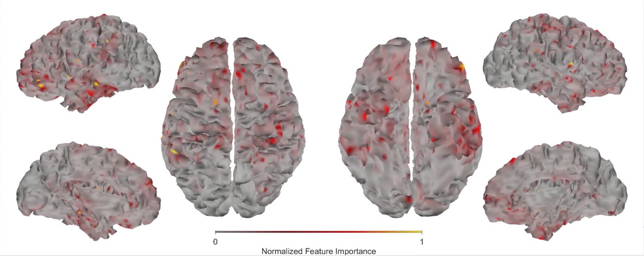
      In response to Reviewer 2’s request for deeper interpretation of our findings and stronger theoretical grounding, we have expanded our discussion by incorporating a thorough interpretation of how mental health indices relate to cognition, material that was previously included only in supplementary materials due to word limit constraints. We have further strengthened the theoretical justification for our study design, with particular emphasis on the importance of examining shared variance between cognition and mental health through the derivation of neural markers of cognition. Additionally, to enhance the biological interpretation of our results, we included new analyses of feature importance across neuroimaging modalities, providing clearer insights into which neural features contribute most to the observed relationships.

      Notably, Reviewer 3 acknowledged the strength of our study, including multimodal design, robust analytical approach, and clear visualization and interpretation of results. Their comments were exclusively methodological, underscoring the manuscript’s quality.

      Reviewer 1:

      The authors try to bridge mental health characteristics, global cognition and various MRI-derived (structural, diffusion and resting state fMRI) measures using the large dataset of UK Biobank. Each MRI modality alone explained max 25% of the cognitionmental health covariance, and when combined together 48% of the variance could be explained. As a peer-reviewer not familiar with the used methods (machine learning, although familiar with imaging), the manuscript is hard to read and I wonder what the message for the field might be. In the end of the discussion the authors state '... we provide potential targets for behavioural and physiological interventions that may affect cognition', the real relevance (and impact) of the findings is unclear to me.

      Thank you for your thorough review and practical recommendations. We appreciate your constructive comments and suggestions and hope our revisions adequately address your concerns.

      Major questions

      (1) The methods are hard to follow for people not in this specific subfield, and therefore, I expect that for readers it is hard to understand how valid and how useful the approach is.

      Thank you for your comment. To enhance accessibility for readers without a machine learning background, we revised the Methods section to clarify our analyses while retaining important technical details needed to understand our approach. Recognizing that some concepts may require prior knowledge, we provide detailed explanations of each analysis step, including the machine learning pipeline in the Supplementary Methods.

      Line 188: “We employed nested cross-validation to predict cognition from mental health indices and 72 neuroimaging phenotypes (Fig. 1). Nested cross-validation is a robust method for evaluating machine-learning models while tuning their hyperparameters, ensuring that performance estimates are both accurate and unbiased. Here, we used a nested cross-validation scheme with five outer folds and ten inner folds.

      We started by dividing the entire dataset into five outer folds. Each fold took a turn being held out as the outerfold test set (20% of the data), while the remaining four folds (80% of the data) were used as an outer-fold training set. Within each outer-fold training set, we performed a second layer of cross-validation – this time splitting the data into ten inner folds. These inner folds were used exclusively for hyperparameter tuning: models were trained on nine of the inner folds and validated on the remaining one, cycling through all ten combinations.

      We then selected the hyperparameter configuration that performed best across the inner-fold validation sets, as determined by the minimal mean squared error (MSE). The model was then retrained on the full outer-fold training set using this hyperparameter configuration and evaluated on the outer-fold test set, using four performance metrics: Pearson r, the coefficient of determination ( R<sup>2</sup>), the mean absolute error (MAE), and the MSE. This entire process was repeated for each of the five outer folds, ensuring that every data point is used for both training and testing, but never at the same time. We opted for five outer folds instead of ten to reduce computational demands, particularly memory and processing time, given the substantial volume of neuroimaging data involved in model training. Five outer folds led to an outer-fold test set at least n = 4 000, which should be sufficient for model evaluation. In contrast, we retained ten inner folds to ensure robust and stable hyperparameter tuning, maximising the reliability of model selection.

      To model the relationship between mental health and cognition, we employed Partial Least Squares Regression (PLSR) to predict the g-factor from 133 mental health variables. To model the relationship between neuroimaging data and cognition, we used a two-step stacking approach [15–17,61] to integrate information from 72 neuroimaging phenotypes across three MRI modalities. In the first step, we trained 72 base (first-level) PLSR models, each predicting the g-factor from a single neuroimaging phenotype. In the second step, we used the predicted values from these base models as input features for stacked models, which again predicted the g-factor. We constructed four stacked models based on the source of the base predictions: one each for dwMRI, rsMRI, sMRI, and a combined model incorporating all modalities (“dwMRI Stacked”, “rsMRI Stacked”, “sMRI Stacked”, and “All MRI Stacked”, respectively). Each stacked model was trained using one of four machine learning algorithms – ElasticNet, Random Forest, XGBoost, or Support Vector Regression – selected individually for each model (see Supplementary Materials, S6).

      For rsMRI phenotypes, we treated the choice of functional connectivity quantification method – full correlation, partial correlation, or tangent space parametrization – as a hyperparameter. The method yielding the highest performance on the outer-fold training set was selected for predicting the g-factor (see Supplementary Materials, S5).

      To prevent data leakage, we standardized the data using the mean and standard deviation derived from the training set and applied these parameters to the corresponding test set within each outer fold. This standardization was performed at three key stages: before g-factor derivation, before regressing out modality-specific confounds from the MRI data, and before stacking. Similarly, to maintain strict separation between training and testing data, both base and stacked models were trained exclusively on participants from the outer-fold training set and subsequently applied to the corresponding outer-fold test set.

      To evaluate model performance and assess statistical significance, we aggregated the predicted and observed g_factor values from each outer-fold test set. We then computed a bootstrap distribution of Pearson’s correlation coefficient (_r) by resampling with replacement 5 000 times, generating 95% confidence intervals (CIs) (Fig. 1). Model performance was considered statistically significant if the 95% CI did not include zero, indicating that the observed associations were unlikely to have occurred by chance.”

      (2) If only 40% of the cognition-mental health covariation can be explained by the MRI variables, how to explain the other 60% of the variance? And related to this %: why do the author think that 'this provides us confidence in using MRI to derive quantitative neuromarkers of cognition'?

      Thank you for this insightful observation. Using the MRI modalities available in the UK Biobank, we were able to account for 48% of the covariation between cognition and mental health. The remaining 52% of unexplained variance may arise from several sources. One possibility is the absence of certain neuroimaging modalities in the UK Biobank dataset, such as task-based fMRI contrasts, positron emission tomography, arterial spin labeling, and magnetoencephalography/electroencephalography. Prior research from our group and others has consistently demonstrated strong predictive performance from specific task-based fMRI contrasts, particularly those derived from tasks like the n-Back working memory task and the face-name episodic memory task, none of which is available in the UK Biobank.

      Moreover, there are inherent limitations in using MRI as a proxy for brain structure and function. Measurement error and intra-individual variability, such as differences in a cognitive state between cognitive assessments and MRI acquisition, may also contribute to the unexplained variance. According to the Research Domain Criteria (RDoC) framework, brain circuits represent only one level of neurobiological analysis relevant to cognition. Other levels, including genes, molecules, cells, and physiological processes, may also play a role in the cognition-mental health relationship.

      Nonetheless, neuroimaging provides a valuable window into the biological mechanisms underlying this overlap – insights that cannot be gleaned from behavioural data alone. We have now incorporated these considerations into the Discussion section.

      Line 658: “Although recent debates [18] have challenged the predictive utility of MRI for cognition, our multimodal marker integrating 72 neuroimaging phenotypes captures nearly half of the mental health-explained variance in cognition. We demonstrate that neural markers with greater predictive accuracy for cognition also better explain cognition-mental health covariation, showing that multimodal MRI can capture both a substantial cognitive variance and nearly half of its shared variance with mental health. Finally, we show that our neuromarkers explain a substantial portion of the age- and sex-related variance in the cognition-mental health relationship, highlighting their relevance in modeling cognition across demographic strata.

      The remaining unexplained variance in the relationship between cognition and mental health likely stems from multiple sources. One possibility is the absence of certain neuroimaging modalities in the UK Biobank dataset, such as task-based fMRI contrasts, positron emission tomography, arterial spin labeling, and magnetoencephalography/electroencephalography. Prior research has consistently demonstrated strong predictive performance from specific task-based fMRI contrasts, particularly those derived from tasks like the n-Back working memory task and the face-name episodic memory task, none of which is available in the UK Biobank [15,17,61,69,114,142,151].

      Moreover, there are inherent limitations in using MRI as a proxy for brain structure and function. Measurement error and intra-individual variability, such as differences in a cognitive state between cognitive assessments and MRI acquisition, may also contribute to the unexplained variance. According to the RDoC framework, brain circuits represent only one level of neurobiological analysis relevant to cognition [14]. Other levels, including genes, molecules, cells, and physiological processes, may also play a role in the cognition-mental health relationship.

      Nonetheless, neuroimaging provides a valuable window into the biological mechanisms underlying this overlap – insights that cannot be gleaned from behavioural data alone. Ultimately, our findings validate brain-based neural markers as a fundamental neurobiological unit of analysis, advancing our understanding of mental health through the lens of cognition.”

      Regarding our confidence in using MRI to derive neural markers for cognition, we base this on the predictive performance of MRI-based models. As we note in the Discussion (Line 554: “Consistent with previous studies, we show that MRI data predict individual differences in cognition with a medium-size performance (r ≈ 0.4) [15–17, 28, 61, 67, 68].”), the medium effect size we observed (r ≈ 0.4) agrees with existing literature on brain-cognition relationships, confirming that machine learning leads to replicable results. This effect size represents a moderate yet meaningful association in neuroimaging studies of aging, consistent with reports linking brain to behaviour in adults (Krämer et al., 2024; Tetereva et al., 2022). For example, a recent meta-analysis by Vieira and colleagues (2022) reported a similar effect size (r = 0.42, 95% CI [0.35;0.50]). Our study includes over 15000 participants, comparable to or more than typical meta-analyses, allowing us to characterise our work as a “mega-analysis”. And on top of this predictive performance, we found our neural markers for cognition to capture half of the cognition-mental health covariation, boosting our confidence in our approach.

      Krämer C, Stumme J, da Costa Campos L, Dellani P, Rubbert C, Caspers J, et al. Prediction of cognitive performance differences in older age from multimodal neuroimaging data. GeroScience. 2024;46:283–308.

      Tetereva A, Li J, Deng JD, Stringaris A, Pat N. Capturing brain cognition relationship: Integrating task‐based fMRI across tasks markedly boosts prediction and test‐retest reliability. NeuroImage. 2022;263:119588.

      (3) Imagine that we can increase the explained variance using multimodal MRI measures, why is it useful? What does it learn us? What might be the implications?

      We assume that by variance, Reviewer 1 referred to the cognition-mental health covariation mentioned in point 2) above.

      If we can increase the explained cognition-mental health covariation using multimodal MRI measures, it would mean that we have developed a reasonable neuromarker that is close to RDoC’s neurobiological unit of analysis for cognition. RDoC treats cognition as one of the main basic functional domains that transdiagnostically underly mental health. According to RDoC, mental health should be studied in relation to cognition, alongside other domains such as negative and positive valence systems, arousal and regulatory systems, social processes, and sensorimotor functions. RDoC further emphasizes that each domain, including cognition, should be investigated not only at the behavioural level but also through its neurobiological correlates. This means RDoC aims to discover neural markers of cognition that explain the covariation between cognition and mental health. For us, we approach the development of such neural markers using multimodal neuroimaging. We have now explained the motivation of our study in the first paragraph of the Introduction.

      Line 43: “Cognition and mental health are closely intertwined [1]. Cognitive dysfunction is present in various mental illnesses, including anxiety [2, 3], depression [4–6], and psychotic disorders [7–12]. National Institute of Mental Health’s Research Domain Criteria (RDoC) [13,14] treats cognition as one of the main basic functional domains that transdiagnostically underly mental health. According to RDoC, mental health should be studied in relation to cognition, alongside other domains such as negative and positive valence systems, arousal and regulatory systems, social processes, and sensorimotor functions. RDoC further emphasizes that each domain, including cognition, should be investigated not only at the behavioural level but also through its neurobiological correlates. In this study, we aim to examine how the covariation between cognition and mental health is reflected in neural markers of cognition, as measured through multimodal neuroimaging.”

      More specific issues:

      Introduction

      (4) In the intro the sentence 'in some cases, altered cognitive functioning is directly related to psychiatric symptom severity' is in contrast to the next sentence '... are often stable and persist upon alleviation of psychiatric symptoms'.

      Thank you for pointing this out. The first sentence refers to cases where cognitive deficits fluctuate with symptom severity, while the second emphasizes that core cognitive impairments often remain stable even during symptom remission. To avoid this confusion, we have removed these sentences.

      (5) In the intro the text on the methods (various MRI modalities) is not needed for the Biol Psych readers audience.

      We appreciate your comment. While some members of our target audience may have backgrounds in neuroimaging, machine learning, or psychiatry, we recognize that not all readers will be familiar with all three areas. To ensure accessibility for those who are not familiar with neuroimaging, we included a brief overview of the MRI modalities and quantification methods used in our study to provide context for the specific neuroimaging phenotypes. Additionally, we provided background information on the machine learning techniques employed, so that readers without a strong background in machine learning can still follow our methodology.

      (6) Regarding age of the study sample: I understand that at recruitment the subjects' age ranges from 40 to 69 years. At MRI scanning the age ranges between about 46 to 82. How is that possible? And related to the age of the population: how did the authors deal with age in the analyses, since age is affecting both cognition as the brain measures?

      Thank you for noticing this. In the Methods section, we first outline the characteristics of the UK Biobank cohort, including the age at first recruitment (40-69 years). Table 1 then shows the characteristics of participant subsamples included in each analysis. Since our study used data from Instance 2 (the second in-person visit), participants were approximately 5-13 years older at scanning, resulting in the age range of 46 to 82 years. We clarified the Table 1 caption as follows:

      Line 113: “Table 1. Demographics for each subsample analysed: number, age, and sex of participants who completed all cognitive tests, mental health questionnaires, and MRI scanning”

      We acknowledge that age may influence cognitive and neuroimaging measures. In our analyses, we intentionally preserved age-related variance in brain-cognition relationships across mid and late adulthood, as regressing out age completely would artificially remove biologically meaningful associations. At the same time, we rigorously addressed the effects of age and sex through additional commonality analyses quantifying age and sex contributions to the relationship between cognition and mental health.

      As noted by Reviewer 1 and illustrated in Figure 8, age and sex shared substantial overlapping variance with both mental health and neuroimaging phenotypes in explaining cognitive outcomes. For example, in Figure 8i, age and sex together accounted for 43% of the variance in the cognition-mental health relationship:

      (2.76 + 1.03) / (2.76 + 1.03 + 3.52 + 1.45) ≈ 0.43

      Furthermore, neuromarkers from the all-MRI stacked model explained 72% of this age/sexrelated variance:

      2.76 / (2.76 + 1.03) ≈ 0.72

      This indicates that our neuromarkers captured a substantial portion of the cognition-mental health covariation that varied with age and sex, highlighting their relevance in age/sex-sensitive cognitive modeling.

      In the Methods, Results, and Discussion, we say:

      Methods

      Line 263: “To understand how demographic factors, including age and sex, contribute to this relationship, we also conducted a separate set of commonality analyses treating age, sex, age2, age×sex, and age2×sex as an additional set of explanatory variables (Fig. 1).”

      Results

      Line 445: “Age and sex shared substantial overlapping variance with both mental health and neuroimaging in explaining cognition, accounting for 43% of the variance in the cognition-mental health relationship. Multimodal neural marker of cognition based on three MRI modalities (“All MRI Stacked”) explained 72% of this age and sex-related variance (Fig. 8i–l and Table S21).”

      Discussion

      Line 660: “We demonstrate that neural markers with greater predictive accuracy for cognition also better explain cognition-mental health covariation, showing that multimodal MRI can capture both a substantial cognitive variance and nearly half of its shared variance with mental health. Finally, we show that our neuromarkers explain a substantial portion of the age- and sex-related variance in the cognition-mental health relationship, highlighting their relevance in modeling cognition across demographic strata.”

      (7) Regarding the mental health variables: where characteristics with positive value (e.g. happiness and subjective wellbeing) reversely scored (compared to the negative items, such as anxiety, addition, etc)?

      We appreciate you noting this. These composite scores primarily represent standard clinical measures such as the GAD-7 anxiety scale and N-12 neuroticism scale. We did not reverse the scores to keep their directionality, therefore making interpretability consistent with the original studies the scores were derived from (e.g., Davis et al., 2020; Dutt et al., 2022). Complete descriptive statistics for all mental health indices and detailed derivation procedures are provided in the Supplementary Materials (S2). On Page 6, Supplementary Methods, we say:

      Line 92: “Composite mental health scores included the Generalized Anxiety Disorder (GAD-7), the Posttraumatic Stress Disorder (PTSD) Checklist (PCL-6), the Alcohol Use Disorders Identification Test (AUDIT), the Patient Health Questionnaire (PHQ-9) [12], the Eysenck Neuroticism (N-12), Probable Depression Status (PDS), and the Recent Depressive Symptoms (RDS-4) scores [13, 14]. To calculate the GAD-7, PCL-6, AUDIT, and PHQ-9, we used questions introduced at the online follow-up [12]. To obtain the N-12, PDS, and RDS-4 scores [14], we used data collected during the baseline assessment [13, 14].

      We subcategorized depression and GAD based on frequency, current status (ever had depression or anxiety and current status of depression or anxiety), severity, and clinical diagnosis (depression or anxiety confirmed by a healthcare practitioner). Additionally, we differentiated between different depression statuses, such as recurrent depression, depression triggered by loss, etc. Variables related to self-harm were subdivided based on whether a person has ever self-harmed with the intent to die.

      To make response scales more intuitive, we recorded responses within the well-being domain such that the lower score corresponded to a lesser extent of satisfaction (“Extremely unhappy”) and the higher score indicated a higher level of happiness (“Extremely happy”). For all questions, we assigned the median values to “Prefer not to answer” (-818 for in-person assessment and -3 for online questionnaire) and “Do not know” (-121 for in-person assessment and -1 for online questionnaire) responses. We excluded the “Work/job satisfaction” question from the mental health derivatives list because it included a “Not employed” response option, which could not be reasonably coded.

      To calculate the risk of PTSD, we used questions from the PCL-6 questionnaire. Following Davis and colleagues [12], PCL-6 scores ranged from 6 to 29. A PCL-6 score of 12 or below corresponds to a low risk of meeting the Clinician-Administered PTSD Scale diagnostic criteria. PCL-6 scores between 13 and 16 and between 17 and 25 are indicative of an increased risk and high risk of PTSD, respectively. A score of above 26 is interpreted as a very high risk of PTSD [12, 15]. PTSD status was set to positive if the PCL-6 score exceeded or was equal to 14 and encompassed stressful events instead of catastrophic trauma alone [12].

      To assess alcohol consumption, alcohol dependence, and harm associated with drinking, we calculated the sum of the ten questions from the AUDIT questionnaire [16]. We additionally subdivided the AUDIT score into the alcohol consumption score (questions 1-3, AUDIT-C) and the score reflecting problems caused by alcohol (questions 4-10, AUDIT-P) [17]. In questions 2-10 that followed the first trigger question (“Frequency of drinking alcohol”), we replaced missing values with 0 as they would correspond to a “Never” response to the first question.

      An AUDIT score cut-off of 8 suggests moderate or low-risk alcohol consumption, and scores of 8 to 15 and above 15 indicate severe/harmful and hazardous (alcohol dependence or moderate-severe alcohol use disorder) drinking, respectively [16, 18]. Subsequently, hazardous alcohol use and alcohol dependence status correspond to AUDIT scores of ≥ 8 and ≥ 15, respectively. The “Alcohol dependence ever” status was set to positive if a participant had ever been physically dependent on alcohol. To reduce skewness, we logx+1-transformed the AUDIT, AUDIT-C, and AUDIT-P scores [17].”

      Davis KAS, Coleman JRI, Adams M, Allen N, Breen G, Cullen B, et al. Mental health in UK Biobank – development, implementation and results from an online questionnaire completed by 157 366 participants: a reanalysis. BJPsych Open. 2020;6:e18.

      Dutt RK, Hannon K, Easley TO, Griffis JC, Zhang W, Bijsterbosch JD. Mental health in the UK Biobank: A roadmap to selfreport measures and neuroimaging correlates. Hum Brain Mapp. 2022;43:816–832.  

      (8) In the discussion section (page 23, line 416-421), the authors refer to specific findings that are not described in the results section > I would add these findings to the main manuscript (including the discussion / interpretation).

      We appreciate your careful reading. We agree that our original Results section did not explicitly describe the factor loadings for mental health in the PLSR model, despite discussing their implications later in the paper. We needed to include this part of the discussion in the Supplementary Materials to meet the word limit of the original submission. However, in response to your suggestion, we have now added the results regarding factor loadings to the Results section. We also moved the discussion of the association between mental health features and general cognition from the Supplementary Material to the manuscript’s Discussion.

      Results

      Line 298: “On average, information about mental health predicted the g-factor at  R<sup>2</sup><sub>mean</sub> = 0.10 and r<sub>mean</sub> \= 0.31 (95% CI [0.291, 0.315]; Fig. 2b and 2c and Supplementary Materials, S9, Table S12). The magnitude and direction of factor loadings for mental health in the PLSR model allowed us to quantify the contribution of individual mental health indices to cognition. Overall, the scores for mental distress, alcohol and cannabis use, and self-harm behaviours relate positively, and the scores for anxiety, neurological and mental health diagnoses, unusual or psychotic experiences, happiness and subjective well-being, and negative traumatic events relate negatively to cognition.”

      Discussion

      Line 492: “Factor loadings derived from the PLSR model showed that the scores for mental distress, alcohol and cannabis use, and self-harm behaviours related positively, and the scores for anxiety, neurological and mental health diagnoses, unusual or psychotic experiences, happiness and subjective well-being, and negative traumatic events related negatively to the g-factor. Positive PLSR loadings of features related to mental distress may indicate greater susceptibility to or exaggerated perception of stressful events, psychological overexcitability, and predisposition to rumination in people with higher cognition [72]. On the other hand, these findings may be specific to the UK Biobank cohort and the way the questions for this mental health category were constructed. In particular, to evaluate mental distress, the UK Biobank questionnaire asked whether an individual sought or received medical help for or suffered from mental distress. In this regard, the estimate for mental distress may be more indicative of whether an individual experiencing mental distress had an opportunity or aspiration to visit a doctor and seek professional help [73]. Thus, people with better cognitive abilities and also with a higher socioeconomic status may indeed be more likely to seek professional help.

      Limited evidence supports a positive association between self-harm behaviours and cognitive abilities, with some studies indicating higher cognitive performance as a risk factor for non-suicidal self-harm. Research shows an inverse relationship between cognitive control of emotion and suicidal behaviours that weakens over the life course [73,74]. Some studies have found a positive correlation between cognitive abilities and the risk of nonsuicidal self-harm, suicidal thoughts, and suicidal plans that may be independent of or, conversely, affected by socioeconomic status [75,76]. In our study, the magnitude of the association between self-harm behaviours and cognition was low (Fig. 2), indicating a weak relationship.

      Positive PLSR loadings of features related to alcohol and cannabis may also indicate the influence of other factors. Overall, this relationship is believed to be largely affected by age, income, education, social status, social equality, social norms, and quality of life [79–80]. For example, education level and income correlate with cognitive ability and alcohol consumption [79,81–83]. Research also links a higher probability of having tried alcohol or recreational drugs, including cannabis, to a tendency of more intelligent individuals to approach evolutionary novel stimuli [84,85]. This hypothesis is supported by studies showing that cannabis users perform better on some cognitive tasks [86]. Alternatively, frequent drinking can indicate higher social engagement, which is positively associated with cognition [87]. Young adults often drink alcohol as a social ritual in university settings to build connections with peers [88]. In older adults, drinking may accompany friends or family visits [89,90]. Mixed evidence on the link between alcohol and drug use and cognition makes it difficult to draw definite conclusions, leaving an open question about the nature of this relationship.

      Consistent with previous studies, we showed that anxiety and negative traumatic experiences were inversely associated with cognitive abilities [90–93]. Anxiety may be linked to poorer cognitive performance via reduced working memory capacity, increased focus on negative thoughts, and attentional bias to threatening stimuli that hinder the allocation of cognitive resources to a current task [94–96]. Individuals with PTSD consistently showed impaired verbal and working memory, visual attention, inhibitory function, task switching, cognitive flexibility, and cognitive control [97–100]. Exposure to traumatic events that did not reach the PTSD threshold was also linked to impaired cognition. For example, childhood trauma is associated with worse performance in processing speed, attention, and executive function tasks in adulthood, and age at a first traumatic event is predictive of the rate of executive function decline in midlife [101,102]. In the UK Biobank cohort, adverse life events have been linked to lower cognitive flexibility, partially via depression level [103].

      In agreement with our findings, cognitive deficits are often found in psychotic disorders [104,105]. We treated neurological and mental health symptoms as predictor variables and did not stratify or exclude people based on psychiatric status or symptom severity. Since no prior studies have examined isolated psychotic symptoms (e.g., recent unusual experiences, hearing unreal voices, or seeing unreal visions), we avoid speculating on how these symptoms relate to cognition in our sample.

      Finally, negative PLSR loadings of the features related to happiness and subjective well-being may be specific to the study cohort, as these findings do not agree with some previous research [107–109]. On the other hand, our results agree with the study linking excessive optimism or optimistic thinking to lower cognitive performance in memory, verbal fluency, fluid intelligence, and numerical reasoning tasks, and suggesting that pessimism or realism indicates better cognition [110]. The concept of realism/optimism as indicators of cognition is a plausible explanation for a negative association between the g-factor and friendship satisfaction, as well as a negative PLSR loading of feelings that life is meaningful, especially in older adults who tend to reflect more on the meaning of life [111]. The latter is supported by the study showing a negative association between cognitive function and the search for the meaning of life and a change in the pattern of this relationship after the age of 60 [112]. Finally, a UK Biobank study found a positive association of happiness with speed and visuospatial memory but a negative relationship with reasoning ability [113].”

      (9) In the discussion section (page 24, line 440-449), the authors give an explanation on why the diffusion measure have limited utility, but the arguments put forward also concern structural and rsfMRI measures.

      Thank you for this important observation. Indeed, the argument about voxel-averaged diffusion components (“… these metrics are less specific to the properties of individual white matter axons or bundles, and instead represent a composite of multiple diffusion components averaged within a voxel and across major fibre pathways”) could theoretically apply across other MRI modalities. We have therefore removed this point from the discussion to avoid overgeneralization. However, we maintain our central argument about the biological specificity of conventional tractography-derived diffusion metrics as their particular sensitivity to white matter microstructure (e.g., axonal integrity, myelin content) may make them better suited for detecting neuropathological changes than dynamic cognitive processes. This interpretation aligns with the mixed evidence linking these metrics to cognitive performance, despite their established utility in detecting white matter abnormalities in clinical populations (e.g., Bergamino et al., 2021; Silk et al., 2009). We clarify this distinction in the manuscript.

      Line 572: “The somewhat limited utility of diffusion metrics derived specifically from probabilistic tractography in serving as robust quantitative neuromarkers of cognition and its shared variance with mental health may stem from their greater sensitivity and specificity to neuronal integrity and white matter microstructure rather than to dynamic cognitive processes. Critically, probabilistic tractography may be less effective at capturing relationships between white matter microstructure and behavioural scores cross-sectionally, as this method is more sensitive to pathological changes or dynamic microstructural alterations like those occurring during maturation. While these indices can capture abnormal white matter microstructure in clinical populations such as Alzheimer’s disease, schizophrenia, or attention deficit hyperactivity disorder (ADHD) [117–119], the empirical evidence on their associations with cognitive performance is controversial [114, 120–126].”

      Bergamino M, Walsh RR, Stokes AM. Free-water diffusion tensor imaging improves the accuracy and sensitivity of white matter analysis in Alzheimer’s disease. Sci Rep. 2021;11:6990.

      Silk TJ, Vance A, Rinehart N, Bradshaw JL, Cunnington R. White-matter abnormalities in attention deficit hyperactivity disorder: a diffusion tensor imaging study. Hum Brain Mapp. 2009;30:2757–2765.

      Reviewer 2:

      This is an interesting study combining a lot of data to investigate the link between cognition and mental health. The description of the study is very clear, it's easy to read for someone like me who does not have a lot of expertise in machine learning.

      We thank you for your thorough review and constructive feedback. Your insightful comments have helped us identify conceptual and methodological aspects that required improvement in the manuscript. We have incorporated relevant changes throughout the paper, and below, we address each of your points in detail.

      Comment 1: My main concern with this manuscript is that it is not yet clear to me what it exactly means to look at the overlap between cognition and mental health. This relation is r=0.3 which is not that high, so why is it then necessary to explain this overlap with neuroimaging measures? And, could it be that the relation between cognition and mental health is explained by third variables (environment? opportunities?). In the introduction I miss an explanation of why it is important to study this and what it will tell us, and in the discussion I would like to read some kind of 'answer' to these questions.

      Thank you. It’s important to clarify why we investigated the relationship between cognition and mental health, and what we found using data from the UK Biobank.

      Conceptually, our work is grounded in the Research Domain Criteria (RDoC; Insel et al., 2010) framework. RDoC conceptualizes mental health not through traditional diagnostic categories, but through core functional domains that span the full spectrum from normal to abnormal functioning. These domains include cognition, negative and positive valence systems, arousal and regulatory systems, social processes, and sensorimotor functions. Within this framework, cognition is considered a fundamental domain that contributes to mental health across diagnostic boundaries. Meta-analytic evidence supports a link between cognitive functioning and mental health (Abramovitch, et al., 2021; East-Richard, et al., 2020). In the context of a large, population-based dataset like the UK Biobank, this implies that cognitive performance – as measured by various cognitive tasks – should be meaningfully associated with available mental health indicators.

      However, because cognition is only one of several functional domains implicated in mental health, we do not expect the covariation between cognition and mental health to be very high. Other domains, such as negative and positive valence systems, arousal and regulatory systems, or social processing, may also play significant roles. Theoretically, this places an upper bound on the strength of the cognition-mental health relationship, especially in normative, nonclinical samples.

      Our current findings from the UK Biobank reflect this. Most of the 133 mental health variables showed relatively weak individual correlations with cognition (mean r \= 0.01, SD = 0.05, min r \= –0.08, max r \= 0.17; see Figure 2). However, using a PLS-based machine learning approach, we were able to integrate information across all mental-health variables to predict cognition, yielding an out-of-sample correlation of r = 0.31 [95% CI: 0.29, 0.32].  

      We believe this estimate approximates the true strength of the cognition-mental health relationship in normative samples, consistent with both theoretical expectations and prior empirical findings. Theoretically, this aligns with the RDoC view that cognition is one of several contributing domains. Empirically, our results are consistent with findings from our previous mega-analysis in children (Wang et al., 2025). Moreover, in the field of gerontology, an effect size of r = 0.31 is not considered small. According to Brydges (2019), it falls around the 70th percentile of effect sizes reported in gerontological studies and approaches the threshold for a large effect (r \= 0.32). Given that most studies report within-sample associations, our out-of-sample results are likely more robust and generalizable (Yarkoni & Westfall, 2017).

      To answer, “why is it then necessary to explain this overlap with neuroimaging measures”, we again draw on the conceptual foundation of the RDoC framework. RDoC emphasizes that each functional domain, such as cognition, should be studied not only at the behavioural level but also across multiple neurobiological units of analysis, including genes, molecules, cells, circuits, physiology, and behaviour.

      MRI-based neural markers represent one such level of analysis. While other biological systems (e.g., genetic, molecular, or physiological) also contribute to the cognition-mental health relationship, neuroimaging provides unique insights into the brain mechanisms underlying this association – insights that cannot be obtained from behavioural data alone.

      In response to the related question, “Could the relationship between cognition and mental health be explained by third variables (e.g., environment, opportunities)?”, we note that developing a neural marker of cognition capable of capturing its relationship with mental health is the central aim of this study. Using the MRI modalities available in the UK Biobank, we were able to account for 48% of the covariation between cognition and mental health.

      The remaining 52% of unexplained variance may stem from several sources. According to the RDoC framework, neuromarkers could be further refined by incorporating additional neuroimaging modalities (e.g., task-based fMRI, PET, ASL, MEG/EEG, fNIRS) and integrating other units of analysis such as genetic, molecular, cellular, and physiological data.

      Once more comprehensive neuromarkers are developed, capturing a greater proportion of the cognition-mental health covariation, they may also lead to new research direction – to investigate how environmental factors and life opportunities influence these markers. However, exploring those environmental contributions lies beyond the scope of the current study.

      We discuss these considerations and explain the motivation of our study in the revised Introduction and Discussion.

      Line 481: “Our analysis confirmed the validity of the g-factor [31] as a quantitative measure of cognition [31], demonstrating that it captures nearly half (39%) of the variance across twelve cognitive performance scores, consistent with prior studies [63–68]. Furthermore, we were able to predict cognition from 133 mental health indices, showing a medium-sized relationship that aligns with existing literature [69,70]. Although the observed mental health-cognition association is lower than within-sample estimates in conventional regression models, it aligns with our prior mega-analysis in children [69]. Notably, this effect size is not considered small in gerontology. In fact, it falls around the 70th percentile of reported effects and approaches the threshold for a large effect at r = 0.32 [71]. While we focused specifically on cognition as an RDoC core domain, the strength of its relationship with mental health may be bounded by the influence of other functional domains, particularly in normative, non-clinical samples – a promising direction for future research.”

      Line 658: “Although recent debates [18] have challenged the predictive utility of MRI for cognition, our multimodal marker integrating 72 neuroimaging phenotypes captures nearly half of the mental health-explained variance in cognition. We demonstrate that neural markers with greater predictive accuracy for cognition also better explain cognition-mental health covariation, showing that multimodal MRI can capture both a substantial cognitive variance and nearly half of its shared variance with mental health. Finally, we show that our neuromarkers explain a substantial portion of the age- and sex-related variance in the cognition-mental health relationship, highlighting their relevance in modeling cognition across demographic strata.

      The remaining unexplained variance in the relationship between cognition and mental health likely stems from multiple sources. One possibility is the absence of certain neuroimaging modalities in the UK Biobank dataset, such as task-based fMRI contrasts, positron emission tomography, arterial spin labeling, and magnetoencephalography/electroencephalography. Prior research has consistently demonstrated strong predictive performance from specific task-based fMRI contrasts, particularly those derived from tasks like the n-Back working memory task and the face-name episodic memory task, none of which is available in the UK Biobank [15,17,61,69,114,142,151].

      Moreover, there are inherent limitations in using MRI as a proxy for brain structure and function. Measurement error and intra-individual variability, such as differences in a cognitive state between cognitive assessments and MRI acquisition, may also contribute to the unexplained variance. According to the RDoC framework, brain circuits represent only one level of neurobiological analysis relevant to cognition [14]. Other levels, including genes, molecules, cells, and physiological processes, may also play a role in the cognition-mental health relationship.

      Nonetheless, neuroimaging provides a valuable window into the biological mechanisms underlying this overlap – insights that cannot be gleaned from behavioural data alone. Ultimately, our findings validate brain-based neural markers as a fundamental neurobiological unit of analysis, advancing our understanding of mental health through the lens of cognition.”

      Introduction

      Line 43: “Cognition and mental health are closely intertwined [1]. Cognitive dysfunction is present in various mental illnesses, including anxiety [2, 3], depression [4–6], and psychotic disorders [7–12]. National Institute of Mental Health’s Research Domain Criteria (RDoC) [13,14] treats cognition as one of the main basic functional domains that transdiagnostically underly mental health. According to RDoC, mental health should be studied in relation to cognition, alongside other domains such as negative and positive valence systems, arousal and regulatory systems, social processes, and sensorimotor functions. RDoC further emphasizes that each domain, including cognition, should be investigated not only at the behavioural level but also through its neurobiological correlates. In this study, we aim to examine how the covariation between cognition and mental health is reflected in neural markers of cognition, as measured through multimodal neuroimaging.”

      Discussion

      Line 481: “Our analysis confirmed the validity of the g-factor [31] as a quantitative measure of cognition [31], demonstrating that it captures nearly half (39%) of the variance across twelve cognitive performance scores, consistent with prior studies [63–68]. Furthermore, we were able to predict cognition from 133 mental health indices, showing a medium-sized relationship that aligns with existing literature [69,70]. Although the observed mental health-cognition association is lower than within-sample estimates in conventional regression models, it aligns with our prior mega-analysis in children [69]. Notably, this effect size is not considered small in gerontology. In fact, it falls around the 70th percentile of reported effects and approaches the threshold for a large effect at r = 0.32 [71]. While we focused specifically on cognition as an RDoC core domain, the strength of its relationship with mental health may be bounded by the influence of other functional domains, particularly in normative, non-clinical samples – a promising direction for future research.”

      Line 658: “Although recent debates [18] have challenged the predictive utility of MRI for cognition, our multimodal marker integrating 72 neuroimaging phenotypes captures nearly half of the mental health-explained variance in cognition. We demonstrate that neural markers with greater predictive accuracy for cognition also better explain cognition-mental health covariation, showing that multimodal MRI can capture both a substantial cognitive variance and nearly half of its shared variance with mental health. Finally, we show that our neuromarkers explain a substantial portion of the age- and sex-related variance in the cognition-mental health relationship, highlighting their relevance in modeling cognition across demographic strata.

      The remaining unexplained variance in the relationship between cognition and mental health likely stems from multiple sources. One possibility is the absence of certain neuroimaging modalities in the UK Biobank dataset, such as task-based fMRI contrasts, positron emission tomography, arterial spin labeling, and magnetoencephalography/electroencephalography. Prior research has consistently demonstrated strong predictive performance from specific task-based fMRI contrasts, particularly those derived from tasks like the n-Back working memory task and the face-name episodic memory task, none of which is available in the UK Biobank [15,17,61,69,114,142,151].

      Moreover, there are inherent limitations in using MRI as a proxy for brain structure and function. Measurement error and intra-individual variability, such as differences in a cognitive state between cognitive assessments and MRI acquisition, may also contribute to the unexplained variance. According to the RDoC framework, brain circuits represent only one level of neurobiological analysis relevant to cognition [14]. Other levels, including genes, molecules, cells, and physiological processes, may also play a role in the cognition-mental health relationship.

      Nonetheless, neuroimaging provides a valuable window into the biological mechanisms underlying this overlap – insights that cannot be gleaned from behavioural data alone. Ultimately, our findings validate brain-based neural markers as a fundamental neurobiological unit of analysis, advancing our understanding of mental health through the lens of cognition.”

      Insel T, Cuthbert B, Garvey M, Heinssen R, Pine DS, Quinn K, et al. Research Domain Criteria (RDoC): Toward a New Classification Framework for Research on Mental Disorders. AJP. 2010;167:748–751.

      Abramovitch, A., Short, T., & Schweiger, A. (2021). The C Factor: Cognitive dysfunction as a transdiagnostic dimension in psychopathology. Clinical Psychology Review, 86, 102007.

      East-Richard, C., R. -Mercier, A., Nadeau, D., & Cellard, C. (2020). Transdiagnostic neurocognitive deficits in psychiatry: A review of meta-analyses. Canadian Psychology / Psychologie Canadienne, 61(3), 190–214.

      Wang Y, Anney R, Pat N. The relationship between cognitive abilities and mental health as represented by cognitive abilities at the neural and genetic levels of analysis. eLife. 2025.14:RP105537.

      Brydges CR. Effect Size Guidelines, Sample Size Calculations, and Statistical Power in Gerontology. Innovation in Aging. 2019;3(4):igz036.

      Yarkoni T, Westfall J. Choosing Prediction Over Explanation in Psychology: Lessons From Machine Learning. Perspect Psychol Sci. 2017;12(6):1100-1122.

      Comment 2 Title: - Shouldn't it be "MRI markers" (plural)?

      We used the singular form (“marker”) intentionally, as it refers to the composite neuroimaging marker derived from all three MRI modalities in our stacked model. This multimodal marker represents the combined predictive power of all modalities and captures the highest proportion of the mental health-cognition relationship in our analyses.

      Comment 3: Introduction - I miss an explanation of why it is useful to look at cognition-mental health covariation

      We believe we have sufficiently addressed this comment in our response to Reviewer 2, comment 1 above.

      Comment 4: - "Demonstrating that MRI-based neural indicators of cognition capture the covariation between cognition and mental health will thereby support the utility of such indicators for understanding the etiology of mental health" (page 4, line 56-58) - how/why?

      Previous research has largely focused on developing MRI-based neural indicators that accurately predict cognitive performance (Marek et al., 2022; Vieira et al., 2020). Building on this foundation, our findings further demonstrate that the predictive performance of a neural indicator for cognition is closely tied to its ability to explain the covariation between cognition and mental health. In other words, the robustness of a neural indicator – its capacity to capture individual differences in cognition – is strongly associated with how well it reflects the shared variance between cognition and mental health.

      This insight is particularly important within the context of the RDoC framework, which seeks to understand the etiology of mental health through functional domains (such as cognition) and their underlying neurobiological units of analysis (Insel et al., 2010). According to RDoC, for a neural indicator of cognition to be informative for mental health research, it must not only predict cognitive performance but also capture its relationship with mental health.

      Furthermore, RDoC emphasizes the integration of neurobiological measures to investigate the influence of environmental and developmental factors on mental health. In line with this, our neural indicators of cognition may serve as valuable tools in future research aimed at understanding how environmental exposures and developmental trajectories shape mental health outcomes. We discuss this in more detail in the revised Discussion.

      Line 481: “Our analysis confirmed the validity of the g-factor [31] as a quantitative measure of cognition [31], demonstrating that it captures nearly half (39%) of the variance across twelve cognitive performance scores, consistent with prior studies [63–68]. Furthermore, we were able to predict cognition from 133 mental health indices, showing a medium-sized relationship that aligns with existing literature [69,70]. Although the observed mental health-cognition association is lower than within-sample estimates in conventional regression models, it aligns with our prior mega-analysis in children [69]. Notably, this effect size is not considered small in gerontology. In fact, it falls around the 70th percentile of reported effects and approaches the threshold for a large effect at r = 0.32 [71]. While we focused specifically on cognition as an RDoC core domain, the strength of its relationship with mental health may be bounded by the influence of other functional domains, particularly in normative, non-clinical samples – a promising direction for future research.”

      Line 658: “Although recent debates [18] have challenged the predictive utility of MRI for cognition, our multimodal marker integrating 72 neuroimaging phenotypes captures nearly half of the mental health-explained variance in cognition. We demonstrate that neural markers with greater predictive accuracy for cognition also better explain cognition-mental health covariation, showing that multimodal MRI can capture both a substantial cognitive variance and nearly half of its shared variance with mental health. Finally, we show that our neuromarkers explain a substantial portion of the age- and sex-related variance in the cognition-mental health relationship, highlighting their relevance in modeling cognition across demographic strata.

      The remaining unexplained variance in the relationship between cognition and mental health likely stems from multiple sources. One possibility is the absence of certain neuroimaging modalities in the UK Biobank dataset, such as task-based fMRI contrasts, positron emission tomography, arterial spin labeling, and magnetoencephalography/electroencephalography. Prior research has consistently demonstrated strong predictive performance from specific task-based fMRI contrasts, particularly those derived from tasks like the n-Back working memory task and the face-name episodic memory task, none of which is available in the UK Biobank [15,17,61,69,114,142,151].

      Moreover, there are inherent limitations in using MRI as a proxy for brain structure and function. Measurement error and intra-individual variability, such as differences in a cognitive state between cognitive assessments and MRI acquisition, may also contribute to the unexplained variance. According to the RDoC framework, brain circuits represent only one level of neurobiological analysis relevant to cognition [14]. Other levels, including genes, molecules, cells, and physiological processes, may also play a role in the cognition-mental health relationship.

      Nonetheless, neuroimaging provides a valuable window into the biological mechanisms underlying this overlap – insights that cannot be gleaned from behavioural data alone. Ultimately, our findings validate brain-based neural markers as a fundamental neurobiological unit of analysis, advancing our understanding of mental health through the lens of cognition.”

      Marek S, Tervo-Clemmens B, Calabro FJ, Montez DF, Kay BP, Hatoum AS, et al. Reproducible brain-wide association studies require thousands of individuals. Nature. 2022;603:654–660.

      Vieira S, Gong QY, Pinaya WHL, et al. Using Machine Learning and Structural Neuroimaging to Detect First Episode Psychosis: Reconsidering the Evidence. Schizophr Bull. 2020;46(1):17-26.

      Insel T, Cuthbert B, Garvey M, Heinssen R, Pine DS, Quinn K, et al. Research Domain Criteria (RDoC): Toward a New Classification Framework for Research on Mental Disorders. AJP. 2010;167:748–751.

      Comment 5: - The explanation about the stacking approach is not yet completely clear to me. I don't understand how the target variable can be the dependent variable in both step one and two. Or are those different variables? It would be helpful to also give an example of the target variable in line 88 on page 5

      Thank you for this excellent question. In our stacking approach, the same target variable, the g-factor, is indeed used across both modeling stages, but with a key distinction in how predictions are generated and integrated.

      In the first-level models, we trained separate Partial Least Squares Regression (PLSR) models for each of the 72 neuroimaging phenotypes, each predicting the g-factor independently. The predicted values from these 72 models were then used as input features for the second-level stacked model, which combined them to generate a final prediction of the g-factor. This twostage framework enables us to integrate information across multiple imaging modalities while maintaining a consistent prediction target.

      To avoid data leakage, both modeling stages were conducted entirely within the training set for each cross-validation fold. Only after the second-level model was trained was it applied to the outer-fold test participants who were not involved in any part of the model training process.

      To improve accessibility, we have revised the Methods section (see Page 10) to clarify this approach, ensuring that the description remains technically accurate while being easier to follow.

      Line 188: “We employed nested cross-validation to predict cognition from mental health indices and 72 neuroimaging phenotypes (Fig. 1). Nested cross-validation is a robust method for evaluating machine-learning models while tuning their hyperparameters, ensuring that performance estimates are both accurate and unbiased. Here, we used a nested cross-validation scheme with five outer folds and ten inner folds.

      We started by dividing the entire dataset into five outer folds. Each fold took a turn being held out as the outerfold test set (20% of the data), while the remaining four folds (80% of the data) were used as an outer-fold training set. Within each outer-fold training set, we performed a second layer of cross-validation – this time splitting the data into ten inner folds. These inner folds were used exclusively for hyperparameter tuning: models were trained on nine of the inner folds and validated on the remaining one, cycling through all ten combinations.

      We then selected the hyperparameter configuration that performed best across the inner-fold validation sets, as determined by the minimal mean squared error (MSE). The model was then retrained on the full outer-fold training set using this hyperparameter configuration and evaluated on the outer-fold test set, using four performance metrics: Pearson r, the coefficient of determination ( R<sup>2</sup>), the mean absolute error (MAE), and the MSE. This entire process was repeated for each of the five outer folds, ensuring that every data point is used for both training and testing, but never at the same time. We opted for five outer folds instead of ten to reduce computational demands, particularly memory and processing time, given the substantial volume of neuroimaging data involved in model training. Five outer folds led to an outer-fold test set at least n = 4 000, which should be sufficient for model evaluation. In contrast, we retained ten inner folds to ensure robust and stable hyperparameter tuning, maximising the reliability of model selection.

      To model the relationship between mental health and cognition, we employed Partial Least Squares Regression (PLSR) to predict the g-factor from 133 mental health variables. To model the relationship between neuroimaging data and cognition, we used a two-step stacking approach [15–17,61] to integrate information from 72 neuroimaging phenotypes across three MRI modalities. In the first step, we trained 72 base (first-level) PLSR models, each predicting the g-factor from a single neuroimaging phenotype. In the second step, we used the predicted values from these base models as input features for stacked models, which again predicted the g-factor. We constructed four stacked models based on the source of the base predictions: one each for dwMRI, rsMRI, sMRI, and a combined model incorporating all modalities (“dwMRI Stacked”, “rsMRI Stacked”, “sMRI Stacked”, and “All MRI Stacked”, respectively). Each stacked model was trained using one of four machine learning algorithms – ElasticNet, Random Forest, XGBoost, or Support Vector Regression – selected individually for each model (see Supplementary Materials, S6).

      For rsMRI phenotypes, we treated the choice of functional connectivity quantification method – full correlation, partial correlation, or tangent space parametrization – as a hyperparameter. The method yielding the highest performance on the outer-fold training set was selected for predicting the g-factor (see Supplementary Materials, S5).

      To prevent data leakage, we standardized the data using the mean and standard deviation derived from the training set and applied these parameters to the corresponding test set within each outer fold. This standardization was performed at three key stages: before g-factor derivation, before regressing out modality-specific confounds from the MRI data, and before stacking. Similarly, to maintain strict separation between training and testing data, both base and stacked models were trained exclusively on participants from the outer-fold training set and subsequently applied to the corresponding outer-fold test set.

      To evaluate model performance and assess statistical significance, we aggregated the predicted and observed gfactor values from each outer-fold test set. We then computed a bootstrap distribution of Pearson’s correlation coefficient (r) by resampling with replacement 5 000 times, generating 95% confidence intervals (CIs) (Fig. 1). Model performance was considered statistically significant if the 95% CI did not include zero, indicating that the observed associations were unlikely to have occurred by chance.”

      Comment 6: Methods - It's not clear from the text and Figure 1 which 12 scores from 11 tests are being used to derive the g-factor. Figure 1 shows only 8 bullet points with 10 scores in A and 13 tests under 'Cognitive tests' in B. Moreover, Supplement S1 describes 12 tests and 14 measures (Prospective Memory test is in the text but not in Supplementary Table 1).

      Thank you for identifying this discrepancy. In the original Figure 1b and in the Supplementary Methods (S1), the “Prospective Memory” test was accidentally duplicated, while it was present in the Supplementary Table 1 (Line 53, Supplementary Table 1). We have now corrected both figures for consistency. To clarify: Figure 1a presents the global mental health and cognitive domains studied, while Figure 1b now accurately lists 1) the 12 cognitive scores from 11 tests used to derive the g-factor (with the Trail Making Test contributing two measures – numeric and alphabetic trails) and 2) the three main categories of mental health indices used as machine learning features.

      We also corrected the Supplementary Materials to remove the duplicate test from the first paragraph. In Supplementary Table 1, there were 11 tests listed, and for the Trail Making test, we specified in the “Core measures” column that this test had 2 derivative scores: duration to complete the numeric path (Trail 1) and duration to complete the alphabetic path (Trail 2).

      Supplementary Materials, Line 46: “We used twelve scores from the eleven cognitive tests that represented the following cognitive domains: reaction time and processing speed (Reaction Time test), working memory (Numeric Memory test), verbal and numerical reasoning (Fluid Intelligence test), executive function (Trail Making Test), non-verbal fluid reasoning (Matrix Pattern Completion test), processing speed (Symbol Digit Substitution test), vocabulary (Picture Vocabulary test), planning abilities (Tower Rearranging test), verbal declarative memory (Paired Associate Learning test), prospective memory (Prospective Memory test), and visual memory (Pairs Matching test) [1].”

      Comment 7: - For the mental health measures: If I understand correctly, the questionnaire items were used individually, but also to create composite scores. This seems counterintuitive, because I would assume that if the raw data is used, the composite scores would not add additional information to that. When reading the Supplement, it seems like I'm not correct… It would be helpful to clarify the text on page 7 in the main text.

      You raise an excellent observation regarding the use of both individual questionnaire items and composite scores. This dual approach was methodologically justified by the properties of Partial Least Squares Regression (PLSR), our chosen first-level machine learning algorithm, which benefits from rich feature sets and can handle multicollinearity through dimensionality reduction. PLSR transforms correlated features into latent variables, meaning both individual items and composite scores can contribute unique information to the model. We elaborate on PLSR's mathematical principles in Supplementary Materials (S5).

      To directly address this concern, we conducted comparative analyses showing that the PLSR model (a single 80/20% training/test split), incorporating all 133 mental health features (both items and composites), outperformed models using either type alone. The full model achieved superior performance (MSE = 0.458, MAE = 0.537, \= 0.112, Pearson r = 0.336, p-value = 6.936e-112) compared to using only composite scores (93 features; MSE = 0.461, MAE = 0.538, R<sup>2</sup> = 0.107, Pearson r = 0.328, p-value = 5.8e-106) or only questionnaire items (40 features; MSE = 0.499, MAE = 0.561, R<sup>2</sup> = 0.033, Pearson r = 0.184, p-value = 2.53e-33). These results confirm that including both data types provide complementary predictive value. We expand on these considerations in the revised Methods section.

      Line 123: “Mental health measures encompassed 133 variables from twelve groups: mental distress, depression, clinical diagnoses related to the nervous system and mental health, mania (including bipolar disorder), neuroticism, anxiety, addictions, alcohol and cannabis use, unusual/psychotic experiences, traumatic events, selfharm behaviours, and happiness and subjective well-being (Fig. 1 and Tables S4 and S5). We included both selfreport questionnaire items from all participants and composite diagnostic scores computed following Davis et al. and Dutt et al. [35,36] as features in our first-level (for explanation, see Data analysis section) Partial Least Squares Regression (PLSR) model. This approach leverages PLSR’s ability to handle multicollinearity through dimensionality reduction, enabling simultaneous use of granular symptom-level information and robust composite measures (for mental health scoring details, see Supplementary Materials, S2). We assess the contribution of each mental health index to general cognition by examining the direction and magnitude of its PLSR-derived loadings on the identified latent variables”

      Comment 8: - Results - The colors in Figure 4 B are a bit hard to differentiate.

      We have updated Figure 4 to enhance colour differentiation by adjusting saturation and brightness levels, improving visual distinction. For further clarity, we split the original figure into two separate figures.

      Comment 9: - Discussion - "Overall, the scores for mental distress, alcohol and cannabis use, and self-harm behaviours relate positively, and the scores for anxiety, neurological and mental health diagnoses, unusual or psychotic experiences, happiness and subjective well-being, and negative traumatic events relate negatively to cognition," - this seems counterintuitive, that some symptoms relate to better cognition and others relate to worse cognition. Could you elaborate on this finding and what it could mean?

      We appreciate you highlighting this important observation. While some associations between mental health indices and cognition may appear counterintuitive at first glance, these patterns are robust (emerging consistently across both univariate correlations and PLSR loadings) and align with previous literature (e.g., Karpinski et al., 2018; Ogueji et al., 2022). For instance, the positive relationship between cognitive ability and certain mental health indicators like help-seeking behaviour has been documented in other population studies (Karpinski et al., 2018; Ogueji et al., 2022), potentially reflecting greater health literacy and access to care among cognitively advantaged individuals. Conversely, the negative associations with conditions like psychotic experiences mirror established neurocognitive deficits in these domains.

      As was initially detailed in Supplementary Materials (S12) and now expanded in our Discussion, these findings likely reflect complex multidimensional interactions. The positive loadings for mental distress indicators may capture: (1) greater help-seeking behaviour among those with higher cognition and socioeconomic resources, and/or (2) psychological overexcitability and rumination tendencies in high-functioning individuals. These interpretations are particularly relevant to the UK Biobank's assessment methods, where mental distress items focused on medical help-seeking rather than symptom severity per se (e.g., as a measure of mental distress, the UK Biobank questionnaire asked whether an individual sought or received medical help for or suffered from mental distress).

      Line 492: “Factor loadings derived from the PLSR model showed that the scores for mental distress, alcohol and cannabis use, and self-harm behaviours related positively, and the scores for anxiety, neurological and mental health diagnoses, unusual or psychotic experiences, happiness and subjective well-being, and negative traumatic events related negatively to the g-factor. Positive PLSR loadings of features related to mental distress may indicate greater susceptibility to or exaggerated perception of stressful events, psychological overexcitability, and predisposition to rumination in people with higher cognition [72]. On the other hand, these findings may be specific to the UK Biobank cohort and the way the questions for this mental health category were constructed. In particular, to evaluate mental distress, the UK Biobank questionnaire asked whether an individual sought or received medical help for or suffered from mental distress. In this regard, the estimate for mental distress may be more indicative of whether an individual experiencing mental distress had an opportunity or aspiration to visit a doctor and seek professional help [73]. Thus, people with better cognitive abilities and also with a higher socioeconomic status may indeed be more likely to seek professional help.

      Limited evidence supports a positive association between self-harm behaviours and cognitive abilities, with some studies indicating higher cognitive performance as a risk factor for non-suicidal self-harm. Research shows an inverse relationship between cognitive control of emotion and suicidal behaviours that weakens over the life course [73,74]. Some studies have found a positive correlation between cognitive abilities and the risk of nonsuicidal self-harm, suicidal thoughts, and suicidal plans that may be independent of or, conversely, affected by socioeconomic status [75,76]. In our study, the magnitude of the association between self-harm behaviours and cognition was low (Fig. 2), indicating a weak relationship.

      Positive PLSR loadings of features related to alcohol and cannabis may also indicate the influence of other factors. Overall, this relationship is believed to be largely affected by age, income, education, social status, social equality, social norms, and quality of life [79–80]. For example, education level and income correlate with cognitive ability and alcohol consumption [79,81–83]. Research also links a higher probability of having tried alcohol or recreational drugs, including cannabis, to a tendency of more intelligent individuals to approach evolutionary novel stimuli [84,85]. This hypothesis is supported by studies showing that cannabis users perform better on some cognitive tasks [86]. Alternatively, frequent drinking can indicate higher social engagement, which is positively associated with cognition [87]. Young adults often drink alcohol as a social ritual in university settings to build connections with peers [88]. In older adults, drinking may accompany friends or family visits [89,90]. Mixed evidence on the link between alcohol and drug use and cognition makes it difficult to draw definite conclusions, leaving an open question about the nature of this relationship.

      Consistent with previous studies, we showed that anxiety and negative traumatic experiences were inversely associated with cognitive abilities [90–93]. Anxiety may be linked to poorer cognitive performance via reduced working memory capacity, increased focus on negative thoughts, and attentional bias to threatening stimuli that hinder the allocation of cognitive resources to a current task [94–96]. Individuals with PTSD consistently showed impaired verbal and working memory, visual attention, inhibitory function, task switching, cognitive flexibility, and cognitive control [97–100]. Exposure to traumatic events that did not reach the PTSD threshold was also linked to impaired cognition. For example, childhood trauma is associated with worse performance in processing speed, attention, and executive function tasks in adulthood, and age at a first traumatic event is predictive of the rate of executive function decline in midlife [101,102]. In the UK Biobank cohort, adverse life events have been linked to lower cognitive flexibility, partially via depression level [103].

      In agreement with our findings, cognitive deficits are often found in psychotic disorders [104,105]. We treated neurological and mental health symptoms as predictor variables and did not stratify or exclude people based on psychiatric status or symptom severity. Since no prior studies have examined isolated psychotic symptoms (e.g., recent unusual experiences, hearing unreal voices, or seeing unreal visions), we avoid speculating on how these symptoms relate to cognition in our sample.

      Finally, negative PLSR loadings of the features related to happiness and subjective well-being may be specific to the study cohort, as these findings do not agree with some previous research [107–109]. On the other hand, our results agree with the study linking excessive optimism or optimistic thinking to lower cognitive performance in memory, verbal fluency, fluid intelligence, and numerical reasoning tasks, and suggesting that pessimism or realism indicates better cognition [110]. The concept of realism/optimism as indicators of cognition is a plausible explanation for a negative association between the g-factor and friendship satisfaction, as well as a negative PLSR loading of feelings that life is meaningful, especially in older adults who tend to reflect more on the meaning of life [111]. The latter is supported by the study showing a negative association between cognitive function and the search for the meaning of life and a change in the pattern of this relationship after the age of 60 [112]. Finally, a UK Biobank study found a positive association of happiness with speed and visuospatial memory but a negative relationship with reasoning ability [113].”

      Karpinski RI, Kinase Kolb AM, Tetreault NA, Borowski TB. High intelligence: A risk factor for psychological and physiological overexcitabilities. Intelligence. 2018;66:8–23.

      Ogueji IA, Okoloba MM. Seeking Professional Help for Mental Illness: A Mixed-Methods Study of Black Family Members in the UK and Nigeria. Psychol Stud. 2022;67:164–177.

      Comment 10: - All neuroimaging factors together explain 48% of the variance in the cognition-mental health relationship. However, this relationship is only r=0.3 - so then the effect of neuroimaging factors seems a lot smaller… What does it mean?

      Thank you for raising this critical point. We have addressed this point in our response to Reviewer 1, comment 2, Reviewer 1, comment 3 and Reviewer 2, comment 1.

      Briefly, cognition is related to mental health at around r = 0.3 and to neuroimaging phenotypes at around r = 0.4. These levels of relationship strength are consistent to what has been shown in the literature (e.g., Wang et al., 2025 and Vieira et al., 2020). We discussed the relationship between cognition and mental health in our response to Reviewer 2, comment 1 above. In short, this relationship reflects just one functional domain – mental health may also be associated with other domains such as negative and positive valence systems, arousal and regulatory systems, social processes, and sensorimotor functions. Moreover, in the context of gerontology research, this effect size is considered relatively large (Brydges et al., 2019).

      We conducted a commonality analysis to investigate the unique and shared variance of mental health and neuroimaging phenotypes in explaining cognition.  As we discussed in our response to Reviewer 1, comment 2, we were able to account for 48% of the covariation between cognition and mental health using the MRI modalities available in the UK Biobank. The remaining 52% of unexplained variance may arise from several sources.

      One possibility is the absence of certain neuroimaging modalities in the UK Biobank dataset, such as task-based fMRI contrasts, positron emission tomography, arterial spin labeling, and magnetoencephalography/electroencephalography. Prior research from our group and others has consistently demonstrated strong predictive performance from specific task-based fMRI contrasts, particularly those derived from tasks like the n-Back working memory task and the face-name episodic memory task, none of which is available in the UK Biobank (Tetereva et al., 2025).

      Moreover, there are inherent limitations in using MRI as a proxy for brain structure and function. Measurement error and intra-individual variability, such as differences in a cognitive state between cognitive assessments and MRI acquisition, may also contribute to the unexplained variance. According to RDoC framework, brain circuits represent only one level of neurobiological analysis relevant to cognition. Other levels, including genes, molecules, cells, and physiological processes, may also play a role in the cognition-mental health relationship.

      We have now incorporated these considerations into the Discussion section.

      Line 481: “Our analysis confirmed the validity of the g-factor [31] as a quantitative measure of cognition [31], demonstrating that it captures nearly half (39%) of the variance across twelve cognitive performance scores, consistent with prior studies [63–68]. Furthermore, we were able to predict cognition from 133 mental health indices, showing a medium-sized relationship that aligns with existing literature [69,70]. Although the observed mental health-cognition association is lower than within-sample estimates in conventional regression models, it aligns with our prior mega-analysis in children [69]. Notably, this effect size is not considered small in gerontology. In fact, it falls around the 70th percentile of reported effects and approaches the threshold for a large effect at r = 0.32 [71]. While we focused specifically on cognition as an RDoC core domain, the strength of its relationship with mental health may be bounded by the influence of other functional domains, particularly in normative, non-clinical samples – a promising direction for future research.”

      Line 658: “Although recent debates [18] have challenged the predictive utility of MRI for cognition, our multimodal marker integrating 72 neuroimaging phenotypes captures nearly half of the mental health-explained variance in cognition. We demonstrate that neural markers with greater predictive accuracy for cognition also better explain cognition-mental health covariation, showing that multimodal MRI can capture both a substantial cognitive variance and nearly half of its shared variance with mental health. Finally, we show that our neuromarkers explain a substantial portion of the age- and sex-related variance in the cognition-mental health relationship, highlighting their relevance in modeling cognition across demographic strata.

      The remaining unexplained variance in the relationship between cognition and mental health likely stems from multiple sources. One possibility is the absence of certain neuroimaging modalities in the UK Biobank dataset, such as task-based fMRI contrasts, positron emission tomography, arterial spin labeling, and magnetoencephalography/electroencephalography. Prior research has consistently demonstrated strong predictive performance from specific task-based fMRI contrasts, particularly those derived from tasks like the n-Back working memory task and the face-name episodic memory task, none of which is available in the UK Biobank [15,17,61,69,114,142,151].

      Moreover, there are inherent limitations in using MRI as a proxy for brain structure and function. Measurement error and intra-individual variability, such as differences in a cognitive state between cognitive assessments and MRI acquisition, may also contribute to the unexplained variance. According to the RDoC framework, brain circuits represent only one level of neurobiological analysis relevant to cognition [14]. Other levels, including genes, molecules, cells, and physiological processes, may also play a role in the cognition-mental health relationship.

      Nonetheless, neuroimaging provides a valuable window into the biological mechanisms underlying this overlap – insights that cannot be gleaned from behavioural data alone. Ultimately, our findings validate brain-based neural markers as a fundamental neurobiological unit of analysis, advancing our understanding of mental health through the lens of cognition.”

      Wang Y, Anney R, Pat N. The relationship between cognitive abilities and mental health as represented by cognitive abilities at the neural and genetic levels of analysis. eLife. 2025.14:RP105537.

      Vieira S, Gong QY, Pinaya WHL, et al. Using Machine Learning and Structural Neuroimaging to Detect First Episode Psychosis: Reconsidering the Evidence. Schizophr Bull. 2020;46(1):17-26.

      Brydges CR. Effect Size Guidelines, Sample Size Calculations, and Statistical Power in Gerontology. Innovation in Aging. 2019;3(4):igz036.

      Tetereva A, Knodt AR, Melzer TR, et al. Improving Predictability, Reliability and Generalisability of Brain-Wide Associations for Cognitive Abilities via Multimodal Stacking. Preprint. bioRxiv. 2025;2024.05.03.589404.

      Reviewer 3:

      Buianova et al. present a comprehensive analysis examining the predictive value of multimodal neuroimaging data for general cognitive ability, operationalized as a derived g-factor. The study demonstrates that functional MRI holds the strongest predictive power among the modalities, while integrating multiple MRI modalities through stacking further enhances prediction performance. The inclusion of a commonality analysis provides valuable insight into the extent to which shared and unique variance across mental health features and neuroimaging modalities contributes to the observed associations with cognition. The results are clearly presented and supported by highquality visualizations. Limitations of the sample are stated clearly.

      Thank you once more for your constructive and encouraging feedback. We appreciate your careful reading and valuable methodological insights. Your expertise has helped us clarify key methodological concepts and improve the overall rigour of our study.

      Suggestions for improvement:

      (1) The manuscript would benefit from the inclusion of permutation testing to evaluate the statistical significance of the predictive models. This is particularly important given that some of the reported performance metrics are relatively modest, and permutation testing could help ensure that results are not driven by chance.

      Thank you, this is an excellent point. We agree that evaluating the statistical significance of our predictive models is essential.

      In our original analysis, we assessed model performance by generating a bootstrap distribution of Pearson’s r, resampling the data with replacement 5,000 times (see Figure 3b). In response to your feedback, we have made the following updates:

      (1) Improved Figure 3b to explicitly display the 95% confidence intervals.

      (2) Supplemented the results by reporting the exact confidence interval values.

      (3) Clarified our significance testing procedure in the Methods section.

      We considered model performance statistically significant when the 95% confidence interval did not include zero, indicating that the observed associations are unlikely to have occurred by chance.

      We chose bootstrapping over permutation testing because, while both can assess statistical significance, bootstrapping additionally provides uncertainty estimates in the form of confidence intervals. Given the large sample size in our study, significance testing can be less informative, as even small effects may reach statistical significance. Bootstrapping offers a more nuanced understanding of model uncertainty.

      Line 233: “To evaluate model performance and assess statistical significance, we aggregated the predicted and observed g-factor values from each outer-fold test set. We then computed a bootstrap distribution of Pearson’s correlation coefficient (r) by resampling with replacement 5 000 times, generating 95% confidence intervals (CIs) (Fig. 1). Model performance was considered statistically significant if the 95% CI did not include zero, indicating that the observed associations were unlikely to have occurred by chance.”

      (2) Applying and testing the trained models on an external validation set would increase confidence in generalisability of the model.

      We appreciate this excellent suggestion. While we considered this approach, implementing it would require identifying an appropriate external dataset with comparable neuroimaging and behavioural measures, along with careful matching of acquisition protocols and variable definitions across sites. These challenges extend beyond the scope of the current study, though we fully agree that this represents an important direction for future research.

      Our findings, obtained from one of the largest neuroimaging datasets to date with training and test samples exceeding most previous studies, align closely with existing literature: the predictive accuracy of each neuroimaging phenotype and modality for cognition matches the effect size reported in meta-analyses (r ≈ 0.4; e.g., Vieira et al., 2020). The ability of dwMRI, rsMRI and sMRI to capture the cognition-mental health relationship is, in turn, consistent with our previous work in pediatric populations (Wang et al., 2025; Pat et al., 2022).

      Vieira S, Gong QY, Pinaya WHL, et al. Using Machine Learning and Structural Neuroimaging to Detect First Episode Psychosis: Reconsidering the Evidence. Schizophr Bull. 2020;46(1):17-26.

      Wang Y, Anney R, Pat N. The relationship between cognitive abilities and mental health as represented by cognitive abilities at the neural and genetic levels of analysis. eLife. 2025.14:RP105537.

      Pat N, Wang Y, Anney R, Riglin L, Thapar A, Stringaris A. Longitudinally stable, brain-based predictive models mediate the relationships between childhood cognition and socio-demographic, psychological and genetic factors. Hum Brain Mapp. 2022;43:5520–5542.

      (3) The rationale for selecting a 5-by-10-fold cross-validation scheme is not clearly explained. Clarifying why this structure was preferred over more commonly used alternatives, such as 10-by-10 or 5-by-5 cross-validation, would strengthen the methodological transparency.

      Thank you for this important methodological question. Our choice of a 5-by-10-fold crossvalidation scheme was motivated by the need to balance robust hyperparameter tuning with computational efficiency, particularly memory and processing time. Retaining five outer folds allowed us to rigorously assess model performance across multiple data partitions, leading to an outer-fold test set at least n = 4 000 and providing a substantial amount of neuroimaging data involved in model training. In contrast, employing ten inner folds ensured robust and stable hyperparameter tuning that maximizes the reliability of model selection. Thus, the 5-outer-fold with our large sample provided sufficient out-of-sample test set size for reliable model evaluation and efficient computation, while 10 inner folds enabled robust hyperparameter tuning. We now provide additional rationale for this design decision on Page 10.

      Line 188: “We employed nested cross-validation to predict cognition from mental health indices and 72 neuroimaging phenotypes (Fig. 1). Nested cross-validation is a robust method for evaluating machine-learning models while tuning their hyperparameters, ensuring that performance estimates are both accurate and unbiased. Here, we used a nested cross-validation scheme with five outer folds and ten inner folds.

      We started by dividing the entire dataset into five outer folds. Each fold took a turn being held out as the outerfold test set (20% of the data), while the remaining four folds (80% of the data) were used as an outer-fold training set. Within each outer-fold training set, we performed a second layer of cross-validation – this time splitting the data into ten inner folds. These inner folds were used exclusively for hyperparameter tuning: models were trained on nine of the inner folds and validated on the remaining one, cycling through all ten combinations.

      We then selected the hyperparameter configuration that performed best across the inner-fold validation sets, as determined by the minimal mean squared error (MSE). The model was then retrained on the full outer-fold training set using this hyperparameter configuration and evaluated on the outer-fold test set, using four performance metrics: Pearson r, the coefficient of determination ( R<sup>2</sup>), the mean absolute error (MAE), and the MSE. This entire process was repeated for each of the five outer folds, ensuring that every data point is used for both training and testing, but never at the same time. We opted for five outer folds instead of ten to reduce computational demands, particularly memory and processing time, given the substantial volume of neuroimaging data involved in model training. Five outer folds led to an outer-fold test set at least n = 4 000, which should be sufficient for model evaluation. In contrast, we retained ten inner folds to ensure robust and stable hyperparameter tuning, maximising the reliability of model selection.”

      (4) A more detailed discussion of which specific brain regions or features within each neuroimaging modality contributed most strongly to the prediction of cognition would enhance neurobiological relevance of the findings.

      Thank you for this thoughtful suggestion. To address this point, we have included feature importance plots for the top-performing neuroimaging phenotypes within each modality (Figure 5 and Figures S2–S4), demonstrating the relative contributions of individual features to the predictive models. While we maintain our primary focus on cross-modality performance comparisons in the main text, as this aligns with our central aim of evaluating multimodal MRI markers at the integrated level, we outline the contribution of neuroimaging features with the highest predictive performance for cognition in the revised Results and Discussion.

      Methods

      Line 255: “To determine which neuroimaging features contribute most to the predictive performance of topperforming phenotypes within each modality, while accounting for the potential latent components derived from neuroimaging, we assessed feature importance using the Haufe transformation [62]. Specifically, we calculated Pearson correlations between the predicted g-factor and scaled and centred neuroimaging features across five outer-fold test sets. We also examined whether the performance of neuroimaging phenotypes in predicting cognition per se is related to their ability to explain the link between cognition and mental health. Here, we computed the correlation between the predictive performance of each neuroimaging phenotype and the proportion of the cognition-mental health relationship it captures. To understand how demographic factors, including age and sex, contribute to this relationship, we also conducted a separate set of commonality analyses treating age, sex, age<sup>2</sup>, age×sex, and age<sup>2</sup>×sex as an additional set of explanatory variables (Fig. 1).”

      Results

      dwMRI

      Line 331: “Overall, models based on structural connectivity metrics performed better than TBSS and probabilistic tractography (Fig. 3). TBSS, in turn, performed better than probabilistic tractography (Fig. 3 and Table S13). The number of streamlines connecting brain areas parcellated with aparc MSA-I had the best predictive performance among all dwMRI neuroimaging phenotypes (R<sup>2</sup><sub>mean</sub> = 0.052, r<sub>mean</sub> = 0.227, 95% CI [0.212, 0.235]). To identify features driving predictions, we correlated streamline counts in aparc MSA-I parcellation with the predicted g_factor values from the PLSR model. Positive associations with the predicted _g-factor were strongest for left superior parietal-left caudal anterior cingulate, left caudate-right amygdala, and left putamen-left hippocampus connections. The most marked negative correlations involved left putamen-right posterior thalamus and right pars opercularis-right caudal anterior cingulate pathways (Fig. 5 and Supplementary Fig. S2).”

      rsMRI

      Line 353: “Among RSFC metrics for 55 and 21 ICs, tangent parameterization matrices yielded the highest performance in the training set compared to full and partial correlation, as indicated by the cross-validation score. Functional connections between the limbic (IC10) and dorsal attention (IC18) networks, as well as between the ventral attention (IC15) and default mode (IC11) networks, displayed the highest positive association with cognition. In contrast, functional connectivity between the limbic (IC43, the highest activation within network) and default mode (IC11) and limbic (IC45) and frontoparietal (IC40) networks, between the dorsal attention (IC18) and frontoparietal (IC25) networks, and between the ventral attention (IC15) and frontoparietal (IC40) networks, showed the highest negative association with cognition (Fig. 5 and Supplementary Fig. S3 and S4)”

      sMRI

      Line 373: “FreeSurfer subcortical volumetric subsegmentation and ASEG had the highest performance among all sMRI neuroimaging phenotypes (R<sup>2</sup><sub>mean</sub> = 0.068, r<sub>mean</sub> = 0.244, 95% CI [0.237, 0.259] and R<sup>2</sup><sub>mean</sub> = 0.059, r<sub>mean</sub> = 0.235, 95% CI [0.221, 0.243], respectively). In FreeSurfer subcortical volumetric subsegmentation, volumes of all subcortical structures, except for left and right hippocampal fissures, showed positive associations with cognition. The strongest relations were observed for the volumes of bilateral whole hippocampal head and whole hippocampus (Fig. 5 and Supplementary Fig. S5 for feature importance maps). Grey matter morphological characteristics from ex vivo Brodmann Area Maps showed the lowest predictive performance (R<sup>2</sup><sub>mean</sub> = 0.008, r<sub>mean</sub> = 0.089, 95% CI [0.075, 0.098]; Fig. 3 and Table S15).”

      Discussion

      dwMRI

      Line 562: “Among dwMRI-derived neuroimaging phenotypes, models based on structural connectivity between brain areas parcellated with aparc MSA-I (streamline count), particularly connections with bilateral caudal anterior cingulate (left superior parietal-left caudal anterior cingulate, right pars opercularis-right caudal anterior cingulate), left putamen (left putamen-left hippocampus, left putamen-right posterior thalamus), and amygdala (left caudate-right amygdala), result in a neural indicator that best reflects microstructural resources associated with cognition, as indicated by predictive modeling, and more importantly, shares the highest proportion of the variance with mental health-g, as indicated by commonality analysis.”

      rsMRI

      Line 583: “We extend findings on the superior performance of rsMRI in predicting cognition, which aligns with the literature [15, 28], by showing that it also explains almost a third of the variance in cognition that mental health captures. At the rsMRI neuroimaging phenotype level, this performance is mostly driven by RSFC patterns among 55 ICA-derived networks quantified using tangent space parameterization. At a feature level, these associations are best captured by the strength of functional connections among limbic, dorsal attention and ventral attention, frontoparietal and default mode networks. These functional networks have been consistently linked to cognitive processes in prior research [127–130].”

      sMRI

      Line 608: “Integrating information about brain anatomy by stacking sMRI neuroimaging phenotypes allowed us to explain a third of the link between cognition and mental health. Among all sMRI neuroimaging phenotypes, those that quantified the morphology of subcortical structures, particularly volumes of bilateral hippocampus and hippocampal head, explain the highest portion of the variance in cognition captured by mental health. Our findings show that, at least in older adults, volumetric properties of subcortical structures are not only more predictive of individual variations in cognition but also explain a greater portion of cognitive variance shared with mental health than structural characteristics of more distributed cortical grey and white matter. This aligns with the Scaffolding Theory that proposes stronger compensatory engagement of subcortical structures in cognitive processing in older adults [138–140].”

      (5) The formatting of some figure legends could be improved for clarity - for example, some subheadings were not formatted in bold (e.g., Figure 2 c)

      Thank you for noticing this. We have updated the figures to enhance clarity, keeping subheadings plain while bolding figure numbers and MRI modality names.

    1. Réunion pour les parents d'élèves de Terminale Générale au Lycée Louis Vincent : Synthèse et Points Clés

      Cette note de synthèse résume les informations cruciales présentées lors de la réunion des parents d'élèves de terminale générale au Lycée Louis Vincent.

      L'année de terminale est une année charnière, marquée par deux enjeux majeurs : la réussite au baccalauréat et la préparation de l'orientation post-bac via la plateforme Parcoursup.

      Le baccalauréat se compose de 40% de contrôle continu, encadré par un projet d'évaluation strict pour garantir l'équité, et de 60% d'épreuves terminales.

      Le Grand Oral (coefficient 10) représente une opportunité stratégique majeure. Le lycée met en place un programme de préparation intensif avec des devoirs communs et des examens blancs, principalement le samedi matin.


      Parallèlement, le processus Parcoursup est présenté comme un outil indispensable mais complexe, exigeant une préparation dès le début de l'année.

      Les élèves sont invités à utiliser des ressources comme le site SupTracker pour analyser les statistiques d'admission et à consulter les psychologues de l'Éducation nationale (Psy-EN).

      L'accent est mis sur l'importance capitale d'un dossier scolaire solide, où les appréciations des enseignants, l'assiduité et le comportement sont aussi déterminants que les notes.

      La direction insiste sur le fait que, si 100% des élèves de l'établissement ont reçu une proposition sur Parcoursup l'an dernier, l'obtention du vœu prioritaire dépend de l'adéquation entre le projet de l'élève, ses résultats et la qualité de son dossier.


      1. Introduction et Présentation des Acteurs Pédagogiques

      La réunion a débuté par la présentation des équipes pédagogiques et administratives qui encadrent les 299 élèves de terminale générale.

      • Direction :

      • Mme X est Proviseure adjointe en charge du niveau terminale et de la gestion des examens.

      • Mme Z est la nouvelle proviseure adjointe, en charge des niveaux première et BTS.

      • Formations Technologiques et Industrielles :

      • Mme C est Directrice déléguée aux formations (Laboratoire, STL, BTS CIRA, BTS Métiers de la chimie).

      • M. R est Directeur délégué aux formations techniques industrielles, soulignant l'accueil favorable des bacheliers généraux dans les filières BTS.

      • Conseillers Principaux d'Éducation (CPE) : L'équipe de trois CPE, incluant Mme L et Mme B, se partage le suivi des classes de terminale.

      • Professeurs Principaux : Il est précisé qu'un binôme de professeurs principaux est assigné à chaque classe de terminale, l'un se concentrant sur la gestion de la classe et l'autre sur l'orientation, avec une répartition flexible des missions.


      2. Le Baccalauréat 2026 : Modalités d'Évaluation

      L'évaluation du baccalauréat est structurée autour de deux composantes principales, avec un rappel des excellents résultats de l'établissement lors de la session précédente.

      Structure de la Note Finale

      • Le Contrôle Continu représente 40% de la note finale.
      • Les Épreuves Terminales représentent 60% de la note finale.

      Résultats du Lycée Louis-Vincent (Session Juin 2025)

      L'établissement affiche des taux de réussite élevés, témoignant de la qualité de l'accompagnement.

      Voie Générale : Taux de Réussite > 98 %. Voie Générale : Taux de Mention 74 %. Voie Technologique : Taux de Réussite 93 % - 96 %. Voie Technologique : Taux de Mention ≈ 50 %.

      Le Contrôle Continu (40%)

      • Coefficients : L'ensemble des matières suivies en terminale compte pour un total de 19 coefficients dans le calcul du contrôle continu.

      • Projet d'Évaluation : Le lycée a mis en place un projet d'évaluation pour "garantir une égalité de traitement" et des principes communs. *Les moyennes sont validées en conseil de classe et transmises via le Livret Scolaire du Lycéen (LSL).

      • Politique sur les Absences : Une politique stricte est appliquée pour contrer les absences stratégiques visant à éviter une évaluation. Les élèves absents se voient offrir "l'opportunité et non pas la punition" de rattraper les devoirs manqués le samedi matin. Si un élève a trop peu de notes, celles-ci peuvent être jugées "non robustes" par l'Inspection Générale, entraînant une épreuve ponctuelle individuelle pour valider le niveau.

      Les Épreuves Terminales (60%)

      Les épreuves finales se dérouleront principalement en juin. Les coefficients pour la voie générale sont les suivants :

      • Épreuve de Français (passé en Première) : 10 (5 écrit, 5 oral).
      • Épreuve de Philosophie : 8.
      • Épreuve d'Enseignement de Spécialité 1 : 16.
      • Épreuve d'Enseignement de Spécialité 2 : 16.
      • Épreuve du Grand Oral : 10.

      3. Focus sur le Grand Oral

      Le Grand Oral est présenté comme une épreuve d'une importance capitale, tant pour son coefficient que pour les compétences qu'il évalue.

      • Objectifs : Apprendre à s'exprimer en public de façon claire et convaincante, évaluer les capacités d'argumentation, l'esprit critique et les connaissances liées aux deux enseignements de spécialité.

      • Déroulement : Les élèves préparent deux questions. *Le jour de l'épreuve, ils disposent d'un temps de préparation avant un entretien de 20 minutes avec le jury (10 minutes de présentation/réponses et 10 minutes d'échange).

      • Importance Stratégique : Il est souligné que le Grand Oral est une épreuve avec un "rendement de notes" élevé. "Avoir 20 au grand oral c'est possible [...] c'est assez courant", contrairement à d'autres disciplines. C'est donc un levier essentiel pour obtenir une mention ou sécuriser l'obtention du diplôme.


      4. Préparation et Accompagnement au Lycée

      L'établissement organise un calendrier de préparation pour accompagner les élèves vers la réussite.

      • Devoirs Communs et Bacs Blancs : Un calendrier de préparation est en cours de finalisation. *Il inclura des devoirs communs et des bacs blancs, majoritairement organisés le samedi matin.

      • Journées Banalisées : Deux journées seront banalisées en avril (probablement au retour des vacances) pour les épreuves blanches des enseignements de spécialité.

      • Oral Blanc : Un oral blanc sera organisé pour préparer spécifiquement le Grand Oral.

      • Importance de l'Entraînement : La direction insiste sur le fait que s'entraîner en conditions réelles est "indispensable et primordial" pour apprendre à gérer le temps, le stress et l'environnement d'une grande salle d'examen.


      5. L'Orientation et Parcoursup : Un Processus Stratégique

      L'orientation est l'autre grand chantier de l'année, nécessitant une implication précoce et continue des élèves et de leurs familles.

      Événements Clés pour l'Orientation

      • Un Jour à l'Université (UJALU) : En octobre, pendant les vacances. *Les inscriptions débutent le 29 septembre.

      • Salon Oriaction : Les 20, 21 et 22 novembre à Nancy. Le lycée n'organise pas de déplacement collectif ; les familles sont encouragées à s'y rendre, notamment le samedi, pour rencontrer des enseignants du supérieur. Le salon présente 5 000 formations.

      • Forum des formations du Lycée Louis-Vincent : Le 6 février 2025, pour rencontrer étudiants, professionnels et anciens élèves.

      Le Calendrier Parcoursup

      Bien que le calendrier officiel ne soit pas publié, les trois grandes étapes restent les mêmes :

      1. Décembre - Janvier : Ouverture du site avec les informations mises à jour pour la rentrée 2026. Phase d'information.

      2. Mi-Janvier - Mi-Mars : Phase d'inscription et de formulation des vœux. *La date limite de mi-mars est impérative pour ajouter de nouveaux vœux.

      3. Début Juin - Début Juillet : Phase principale d'admission avec réception des réponses des formations.

      Outils et Stratégies pour Parcoursup

      • Ressources Essentielles :

      • Psy-EN : Les élèves, surtout ceux qui sont indécis, sont vivement encouragés à prendre rendez-vous "dès maintenant" avant que les créneaux ne soient saturés.

      • SupTracker : Cet outil statistique est présenté comme "indispensable". Il permet de voir quels profils (spécialités, mentions, notes) ont été admis dans une formation donnée les années précédentes. Par exemple, pour la formation PASS (médecine), 90% des admis en 2025 avaient une combinaison des spécialités Mathématiques, Physique-Chimie ou SVT.

      • Site Parcoursup : La plateforme contient des fiches détaillées sur plus de 24 000 formations, incluant les taux d'accès et les notes moyennes des derniers admis.

      • L'Importance Capitale du Dossier Scolaire :

      • Le proviseur insiste sur le fait que la sélection n'est pas faite par une intelligence artificielle mais par des équipes humaines.

      • Les appréciations des professeurs sont cruciales. *Des remarques comme "travailleur, investi, capable" sont des atouts majeurs.

      • À l'inverse, les absences, les retards et les remarques sur le comportement sont "vraiment très bloquants". *Un dossier avec ces éléments est souvent mis de côté d'emblée par les comités de sélection.

      • Conseils Stratégiques :

      • La devise est : "Il vaut mieux pouvoir choisir qu'être obligé de choisir." Pour cela, il faut que les résultats de l'élève soient à la hauteur de ses ambitions.

      • Il est conseillé d'élargir au maximum le champ des vœux avant la date limite de mi-mars pour ne fermer aucune porte.

      • La phase de résultats en juin est reconnue comme une période de stress intense, notamment à cause des listes d'attente. *Il est rappelé qu'il faut analyser sa position en la comparant au rang du dernier admis de l'année précédente, une information disponible sur Parcoursup.


      6. Questions Diverses

      • Section Euro Allemand / DNL : Cette option est valorisée par une "mention européenne" sur le diplôme du bac. *Les notes et appréciations sont prises en compte dans le dossier Parcoursup et sont visibles par les établissements du supérieur.

      • Heure d'Orientation : L'heure hebdomadaire dédiée à l'orientation n'est pas systématiquement une séance en classe entière. *Il s'agit d'un volume annuel d'environ 10 à 19 séances par professeur principal, qui peuvent prendre la forme de réunions plénières, de travail en petits groupes ou d'entretiens individuels selon les besoins des élèves.

    1. Author response:

      The following is the authors’ response to the original reviews.

      Reviewer #1 (Public Review):

      Summary:

      The paper sets out to examine the social recognition abilities of a 'solitary' jumping spider species. It demonstrates that based on vision alone spiders can habituate and dishabituate to the presence of conspecifics. The data support the interpretation that these spiders can distinguish between conspecifics on the basis of their appearance.

      We appreciate the reviewer’s summary. We indeed aimed at investigating the social recognition abilities of the solitary jumping spider (Phidippus regius), using visual cues alone. By employing a habituation-dishabituation paradigm, well-established in developmental psychology, we found support for the interpretation that these spiders can distinguish between conspecifics based on their appearance, as the reviewer noted.

      Strengths:

      The study presents two experiments. The second set of data recapitulates the findings of the first experiment with an independent set of spiders, highlighting the strength of the results. The study also uses a highly quantitative approach to measuring relative interest between pairs of spiders based on their distance.

      We appreciate the reviewer's acknowledgement of the strengths of our study. The second set of data underscores the robustness and reliability of the results. Additionally, however, the second experiment served the purpose of disentangling whether the habituation effect observed over sessions was caused by ‘physical’ or ‘cognitive’ fatigue by employing ‘long-term’ dishabituation trials at the end of Session 3. These trials are critical in our study as they help to differentiate between recognition of individual identities versus recognition of familiar individuals (as opposed to unfamiliar ones) and to determine if the observed effects are due to ‘general habituation’ or ‘specific recognition’. We will elaborate on this further below in this revision.

      As stated by the reviewer, we employed a highly quantitative approach to measure relative interest between pairs of spiders based on their distance, providing precise and objective data to support our conclusions.

      Weaknesses:

      The study design is overly complicated, missing key controls, and the data presented in the figures are not clearly connected to the study. The discussion is challenging to understand and appears to make unsupported conclusions.

      While we acknowledge that the study design is indeed complex, this complexity is essential for conducting a well-controlled and balanced experiment regarding the experimental conditions.  

      The habituation-dishabituation paradigm is a well-established paradigm in developmental psychology with non-verbal infants. It is understood that during the habituation phase, an individual's attention to a repeated stimulus decreases as they engage in information processing and form a mental representation of it. As the stimulus becomes familiar, it loses its novelty and interest. When a new stimulus is introduced, a recovery of attention suggests that the individual has compared this new stimulus to the stored memory of the habituation stimulus and detected a difference. This process suggests that the individual not only remembered the original stimulus but also recognized the new one as distinct (for a review Kavšek & Bornstein, 2010).

      This paradigm has also been extensively applied in animal research, where, like infants, nonverbal subjects rely on recognition and discrimination processes to demonstrate their cognitive abilities. The use of this paradigm dates back to seminal studies such as Humphrey (1974), which explored the perceptual world of monkeys, illustrating how species and individuals are perceived and recognized. In another previous study (Dahl, Logothetis, and Hoffman, 2007), we utilized an even more complex experimental design that incorporated dedicated baseline trials for both habituation and dishabituation phases, which was well-received despite its complexity. In the current study, we contrast dishabituation and habituation trials directly, creating a sequential cascade where each trial is evaluated against the preceding one as its baseline.

      On the basis of these arguments, we respectfully decline the claim that this paradigm is inappropriate or lacks key controls. Our study design, though complex, is rigorously grounded in established methodologies and offers a robust framework for exploring individual recognition in Phidippus regius.

      However, we take the reviewer’s comments seriously and are committed to identifying and addressing the aspects in our manuscript that may have led to misunderstandings. We clarify these areas in our revision of the manuscript. Modifications were made in the Introduction, Methods, and Discussion sections.

      Dahl, C. D., Logothetis, N. K., & Hoffman, K. L. (2007). Individuation and holistic processing of faces in rhesus monkeys. Proceedings of the Royal Society B: Biological Sciences, 274(1622), 2069-2076.

      Humphrey, N. K. (1974). Species and individuals in the perceptual world of monkeys. Perception, 3(1), 105-114.

      Kavšek, M., & Bornstein, M. H. (2010). Visual habituation and dishabituation in preterm infants: A review and meta-analysis. Research in developmental disabilities, 31(5), 951-975.

      (1) Study design: The study design is rather complicated and as a result, it is difficult to interpret the results. The spiders are presented with the same individual twice in a row, called a habituation trial. Then a new individual is presented twice in a row. The first of these is a dishabituation trial and the second is another habituation trial (but now habituating to a second individual). This is done with three pairings and then this entire structure is repeated over three sessions. 

      While we acknowledge that the design is complex, this complexity is essential for conducting a well-controlled experiment, as described earlier. As the reviewer noted, our design involves presenting the same individual to the focal spider twice in a row (habituation trial), followed by a new individual (dishabituation trial), and then repeating this structure. This approach is fundamental to the habituation-dishabituation paradigm, which allows us to systematically compare the responses to a familiar individual with those elicited by a novel one. If the spiders exhibit different behaviours in terms of the distance they maintain when encountering the same individual versus a new one, it indicates that they are processing the stimuli differently, consistent with recognition memory. This differential response is a key indicator that the spiders can distinguish between familiar and unfamiliar individuals, demonstrating not only a decrease in interest or engagement due to repeated exposure but also a cognitive process where the lack of a matching memory template triggers a distinct behavioural response when confronted with novel stimuli.

      By repeating this sequence two more times (Session 2 and 3), we aim to assess the consistency of this recognition process over time. If the focal spider does not remember the individuals from the previous session (one hour ago), we expect consistent behavioural responses across sessions. Conversely, if there is a decrease in response magnitude but the overall response patterns are maintained, we can infer that the focal spider recognizes the previously presented individuals and exhibits habituation, reflected in reduced response intensity. In other words, over sessions and repeated exposure to the same individuals, the memory traces become more firmly established, leading to a situation where a dishabituation trial introduces less novelty, as the spider's recognition of previously encountered individuals becomes more robust and consistent to the point where “habituation” and “dishabituation” trials become indistinguishable, as observed in Session 3. This method allows us to assess the duration of identity recognition in these spiders, indicating how long the memory of specific individuals persists. 

      All of these outcomes were anticipated before we began Experiment 1. Given that the results aligned with our predictions, we then sought to determine whether the observed reduction in the magnitude of the effect (i.e., the difference between habituation and dishabituation trials) was due to a physical fatigue effect, where the spiders might simply be getting tired, or a cognitive fatigue effect, where the spiders recognized the individuals and as a result did not exhibit any novelty response. To address this, we replicated the experiment with a new group of spiders and introduced special (long-term dishabituation) trials at the end, where the focal spider was presented with a novel spider. 

      These extra trials allowed us to disentangle the nature of the diminishing response across repeated sessions: a lack of dishabituation (remaining distant) would suggest general physical fatigue, whereas a strong dishabituation response (approaching closely) to the novel spider would indicate cognitive fatigue, thereby confirming that the spiders were indeed recognizing the familiar individuals throughout the experiment. 

      In light of these considerations, we believe that the complexity of our design is not only justified but absolutely necessary to rigorously test the cognitive capabilities of the spiders. Nonetheless, we understand the need for clarity in presenting our findings and are committed to refining our manuscript to better communicate the rationale and results of our study.

      The data appear to show the strong effects of differences between habituation and dishabituation trials in the first session. The decrease in differential behavior between the socalled habituation and dishabituation trials in sessions 2 and 3 is explained as a consequence of the spiders beginning to habituate in general to all of the individuals. 

      The key question, as mentioned above, is to determine the underlying cause of this general habituation across sessions. Specifically, we aim to differentiate between two potential causes: physical fatigue, where the spiders may simply become less responsive due to the demands of the three-hour testing period, or cognitive fatigue, where the repeated exposure to the same individuals leads to a decreased response because the spiders have started to recognize these individuals over multiple repetitions.

      To address this, we replicated the experiment and introduced each focal spider to a new individual in what we termed "long-term dishabituation" trials. By comparing the spiders' responses to these novel individuals with their responses in earlier trials, we sought to better understand the underlying mechanisms of habituation and the duration of individual recognition. The strong dishabituation response observed in these trials is indicative of cognitive fatigue, supporting the presence of recognition memory rather than a general physical fatigue effect.

      The claim that the spiders remember specific individuals is somewhat undercut because all of the 'dishabituation' trials in session 2 are toward spiders they already met for 14 minutes previously but seemingly do not remember in session 2. 

      We appreciate the reviewer’s comment regarding the claim that spiders do not remember specific individuals. This assessment does not align with the rationale of our experiment. The reviewer noted that the dishabituation trials in session 2 involved spiders previously encountered and suggested that the lack of a clear memory response might undercut the claim of specific individual recognition. 

      However, as we explained earlier, we expect habituation in Session 2 relative to Session 1 precisely because spiders recognize each other in Session 2. If there were no such habituation in Sessions 2 or 3, it would suggest that the spiders’ recognition memory does not persist beyond one hour. 

      Additionally, it is important to correct the timing noted by the reviewer: each individual spider reencounters the same spider exactly one hour later, not 14 minutes. This is detailed in Table 2 of the manuscript, which outlines that each trial lasts 7 minutes, with a 3-minute visual separation between trials. With six trials per session, this totals to 1 hour per session. Thus, every pair of spiders re-encounters exactly 1 hour after their last interaction.

      Again, it is important to clarify that the observed decrease in differential behaviour is not indicative of a failure to remember specific individuals. Rather, it reflects a systematic pattern of habituation, which is a common and expected outcome in such paradigms. This systematic decrease in response strength suggests that the spiders recognize the previously encountered individuals and becoming less responsive over repeated exposures, consistent with the process of habituation. In different terms, the repeated exposure to the same individuals leads to more firmly established memory traces, leading to a situation where a dishabituation trial introduces less novelty, as the spider's recognition of previously encountered individuals becomes more robust and consistent.

      Based on the explanations provided above, we respectfully reject the claim that “the spiders remember specific individuals is somewhat undercut […]”. In contrast, this claim is incorrect, as the exact opposite is true. The very strength of our study lies in demonstrating that spiders possess robust recognition memory, as evidenced by a clear dissociation of habituation and dishabituation trials in Session 1, followed by a gradually diminishing effect over Session 2 and 3 as the spiders are increased exposed to the same individuals: Furthermore, the strong rebound from habituation observed in long-term dishabituation trials, where the spiders were exposed to novel individuals. 

      This misunderstanding suggests that we should take additional care in the revised manuscript to clarify our explanations and provide more detail, ensuring that the rationale behind our experimental design and findings are communicated effectively.

      In session 3 it is ambiguous what is happening because the spiders no longer differentiate between the trial types. This could be due to fatigue or familiarity. 

      The reviewer proposes that the absence of differentiation between 'habituation' and 'dishabituation' trials in Session 3 might be attributed to either fatigue or familiarity. We interpret "fatigue" as what we have termed the “physical fatigue effect” and "familiarity" as “cognitive fatigue effect.” In this context, we concur with the reviewer’s observation, and this very line of reasoning prompted us to conduct a further experiment following the outcome of Experiment 1.

      A second experiment is done to show that introducing a totally novel individual, recovers a large dishabituation response, suggesting that the lack of differences between 'habituation' and 'dishabituation' trials in session 3 is the result of general habituation to all of the spiders in the session rather than fatigue. As mentioned before, these data do support the claim that spiders differentiate among individuals.

      As the reviewer rightly noted, we addressed these possibilities in our second experiment by introducing a completely novel individual to the spiders, which resulted in a strong dishabituation response. This outcome suggests that the lack of differentiation in Session 3 is more likely due to cognitive habituation rather than physical fatigue. The robust response to novel individuals demonstrates that the spiders are capable of distinguishing between familiar and unfamiliar individuals, suggesting that the reduced differentiation is a consequence of habituation from repeated encounters with the same individuals. 

      We appreciate the reviewer's recognition that these findings support the conclusion that spiders are capable of differentiating between individual conspecifics.

      Additionally, it is important to clarify the structure of our sessions. Each of the 6 trials lasts 7 minutes with a 3-minute visual separation, resulting in a total of 1 hour per session. This ensures that each pair of spiders is encountered exactly one hour later, which controls for the timing and allows us to evaluate the spiders' recognition memory over repeated sessions.

      In summary, while the data show a decrease in differential behaviour between habituation and dishabituation trials in Session 2 and 3, the results from our second experiment support the interpretation that this is due to ‘cognitive habituation’ (familiarization) rather than ‘physical fatigue’ (general habituation). This habituation effect underscores the spiders' ability to recognize and become familiar with specific individuals over time, reinforcing our conclusion that they can differentiate among individuals.

      The data from session 1 are easy to interpret. The data from sessions 2 and 3 are harder to understand, but these are the trials in which they meet an individual again after a substantial period of separation. 

      The data from Session 1 are straightforward to interpret, showing clear differences between habituation and dishabituation trials. However, the data from Sessions 2 and 3 are more complex, as these sessions involve the spiders re-encounter individuals after a 1-hour period of separation. Importantly, the outcome is not an artefact in our experiment, but the consequence of a deliberate choice in the experimental design to assess whether spiders can recognise each other after this duration. We believe that this complexity aligns with our expectations, based on the assumption that spiders can recognise each other after one hour. The observed pattern of habituation in Sessions 2 and 3 suggests that the spiders retain memory of the individuals, leading to decreased responsiveness upon repeated encounters. This interpretation is further supported by the Experiment 2, which introduced a novel individual and elicited a strong dishabituation response. This finding confirms that the reduced differentiation in later sessions is due to cognitive habituation rather than physical fatigue, supporting the conclusion that recognition memory last at least one hour.

      We hope this explanation clarifies our findings and the rationale behind our relatively complex experimental design choice. 

      Other studies looking at recognition in ants and wasps (cited by the authors) have done a 4 trial design in which focal animal A meets B in the first trial, then meets C in the second trial, meets B again in the third trial, and then meets D in the last trial. In that scenario trials 1, 2, and 4 are between unfamiliar individuals and trial 3 is between potentially familiar individuals. In both the ants and wasps, high aggression is seen in species with and without recognition on trial 1, with low aggression specifically for trials with familiar individuals in species with recognition. Across different tests, species or populations that lack recognition have shown a general reduction in aggression towards all individuals that become progressively less aggressive over time (reminiscent of the session 2 and 3 data) while others have maintained modest levels of aggression across all individuals. The 4 session design used in those other studies provides an unambiguous interpretation of the data while controlling for 'fatigue'. 

      We acknowledge that there are multiple ways to design experiments to test recognition memory. In fact, we considered using the paradigm similar to the one proposed by the reviewer and used in studies like Dreier et al., which involves a series of trials with unfamiliar and familiar individuals over extended intervals. We then, however, opted for a more complex design to rigorously assess how habituation and recognition memory develop over repeated sessions with shorter intervals.

      In the following, we would like to describe the advantages and disadvantages of both paradigms and outline how we ended up using the more complex version:

      Advantages of our paradigm: 

      As pointed out, by repeating the sequence in exactly similar manner (every same pair of spiders reoccurs after exactly 1 and 2 hours), we can comprehensively evaluate the effect of habituation over multiple exposures. This allows us to assess the extent of the spiders’ memory, when a spider shows stronger habituation to individuals that were novel in Session 1 but “familiar” by the time they encounter them again in Session 2. To achieve this, we need to ensure that each trial and visual separation is precisely timed, ensuring consistent intervals between encounters. As a consequence, each individual spider undergoes the exact same experimental protocol. Most critically, however, are the novel individuals presented after Session 3 (long-term dishabituation trials) that help differentiate between cognitive habituation and physical fatigue.  Disadvantages of our paradigm:

      The sequences of habituation and dishabituation trials may make the design more complex, as pointed out by the reviewer. As a consequence, the interpretation will become more difficult. However, the data perfectly align with our predictions, and the outcomes were as anticipated in two independently run experiments with two groups of spiders. This highlights the reliability of our experimental design and robustness of our findings.

      Advantages of the 4-trial paradigm proposed by the reviewer:

      Clearly, the structure of the proposed design is simpler, making interpretation easier. The paradigm also accommodates longer intervals between trials (e.g., 24 hours). Longer intervals could theoretically have been applied in our study. (However, we chose not to leave the spiders in the experimental box longer than necessary, opting instead to return them to their home containers for the night to ensure their well-being. And, a 24-hour interval targets a different phase in the process of long-term memory, but more to this topic further below.)

      Disadvantages of the 4-trial paradigm proposed by the reviewer:

      Strictly replicating the 4-trial design would result in one familiar encounter versus three unfamiliar ones. This imbalance might introduce bias and limit the robustness of the measurements. Additionally, the design provides less data overall, as the focal individual will be confronted with three other individuals, who will then be excluded from further testing as focal subjects themselves. In contrast, our design ensures a balanced number of familiar0020(habituation) and novel encounters (dishabituation) for each focal individual, allowing for more efficient and comprehensive data collection without excluding individuals from further testing.

      Given the aforementioned considerations, we determined that the advantages of our experimental design, in particular the assessment of a cognitive fatigue effect when encountering the same individuals again, outweigh those of the proposed 4-trial design. The mentioned limitations of the 4-trial design, such as the potential for bias and less comprehensive data collection, do not justify re-running the study, especially when the best case scenario is fewer insights than our already existing findings. Our current paradigm yielded results that align perfectly with our predictions, offering a thorough and reliable understanding of recognition memory and habituation in spiders. Therefore, we believe our approach provides a more complete and robust answer to our research questions.

      However, we acknowledge that there might be insufficient information in the manuscript addressing the rationale behind our design choices, and we will revise the manuscript to provide a clearer explanation of why our approach is well suited to answering the research questions at hand.

      That all trials in sessions 2 and 3 are always with familiar individuals makes it challenging to understand how much the spiders are habituating to each other versus having some kind of associative learning of individual identity and behavior.

      We understand the reviewer's concern that having all trials in Sessions 2 and 3 involve familiar individuals could make it challenging to distinguish between general habituation and associative learning of individual identities. In our study, we contrast habituation and dishabituation trials: If general habituation were occurring, we would expect uniformly reduced responses (around the zero line) to all individuals over time, indicating that the spiders are getting used to any individual regardless of their specific identity. However, this is not the case. Our data show that while the responses in Session 2 are reduced in effect size compared to Session 1, they are not flat (around the zero line). This indicates that the spiders still differentiate between a repetition of a spider identity (habituation trials) and two different spider identities (dishabituation trials), albeit with a reduced response strength. The systematicity in the data suggests that the spiders are not merely habituating to any individual, but are instead retaining some level of recognition between specific individuals.

      Only by Session 3 do the spiders fully habituate to the point where the responses to habituation and dishabituation trials converge, indicating a complete habituation effect. The introduction of novel individuals in our long-term dishabituation trials further supports the idea that the spiders are recognizing specific individuals rather than exhibiting general habituation. If the spiders were experiencing general habituation, we would not expect the strong dishabituation response observed in our study.

      The data presentation is also very complicated. How is it the case that a negative proportion of time is spent? The methods reveal that this metric is derived by comparing the time individuals spent in each region relative to the previous time they saw that individual. 

      We understand the reviewer's concern regarding the complexity of the data presentation and the calculation of the negative proportion of time. Regarding the complexity of the design, we have already justified our choice of a more intricate experimental setup. This complexity is necessary for accurately assessing recognition memory and habituation over repeated sessions. 

      The metric is derived by comparing the time individuals spent in each region (relative to the transparent front panel) in the current trial (n) relative to the previous trial (n-1). With multiple trials, this results in a cascade of trials and conditions. This method was established in

      Humphrey’s and our previous study (Humphrey, 1974; Dahl, Logothetis, Hoffman, 2007), where we demonstrated its effectiveness in assessing individuation of faces in macaque monkeys.  

      Also in our current experimental design, each current trial is contrasted with the preceding one, allowing us to compare distributions of distances taken in two trials. In this context, every preceding trial serves as baseline for every current trial. 

      Figure 1 of the manuscript, illustrates the structure and analysis of the trials,

      Panel a depicts the baseline, habituation, and dishabituation trials, where spiders are exposed to different conspecifics.

      Baseline (left panel, red): When two spiders are visually exposed to each other for the first time, it is expected that they will explore each other closely, exhibiting high levels of proximity (initial exploratory behaviour).

      Habituation (centre panel, green): When the same spiders are reintroduced in a subsequent round of exposure, it is anticipated that they will exhibit reduced exploratory behaviour and maintain a greater distance compared to the baseline trial, if they recognize each other from the previous encounter (indicative of habituation).

      Panel b (upper and middle panels; red and green): Demonstrates the theoretical assumptions and expected changes in behaviour:

      By subtracting the distribution of distances in the baseline trial from the habituation trial, we generate a delta distribution. This delta distribution reveals negative values near the transparent panel (indicating reduced proximity in the habituation trial) and positive values at mid- to fardistances (indicating increased distancing behaviour). This delta distribution is also what is reported in Figure 2. 

      Dishabituation: In this trial, a new spider (different from the one in the habituation trial) is introduced. The dishabituation trial will be considered in contrast to the habituation trial described above. If the spider recognizes the new individual as different, it is expected to show increased exploratory behaviour and reduced distance, similar to the initial baseline trial.

      By subtracting the distribution of distances in the habituation trial from the dishabituation trial, we obtain another delta distribution. This delta distribution should reveal positive values near the transparent panel (indicating increased proximity in the dishabituation trial) and negative values at mid- to far-distances (indicating decreased proximity compared to the habituation trial).

      We hope this clarifies the rationale behind our data presentation and the methodological approach we employed. We have revised the figure to enhance its clarity and make it more intuitive for the reader.

      Dahl, C. D., Logothetis, N. K., & Hoffman, K. L. (2007). Individuation and holistic processing of faces in rhesus monkeys. Proceedings of the Royal Society B: Biological Sciences, 274(1622), 2069-2076.

      Humphrey, N. K. (1974). Species and individuals in the perceptual world of monkeys. Perception, 3(1), 105-114.

      At the very least, data showing the distribution of distances from the wall would be much easier to interpret for the reader.

      We understand the reviewer's concern that data showing the distribution of distances from the wall would be much easier to interpret for the reader. We initially consider that but came to the conclusion that this approach is not straightforward. For instance, if both spiders are positioned at the very front but in different corners, the distance to the panel would be very small, but the distance between the spiders would be large. Thus, using distances from the wall could misrepresent the actual spatial distribution between the spiders.

      (2) "Long-term social memory": It is not entirely clear what is meant by the authors when they say 'long-term social memory', though typically long-term memory refers to a form of a memory that requires protein synthesis.  

      To address this conceptually, we used the term "long-term social memory" to describe the spiders' ability to recognize and remember individual conspecifics over multiple experimental sessions. While social memory refers to the ability of an individual to recognize other individuals within a social context, long-term memory typically involves the retention of information over extended periods. Recognizing that the term “long-term social memory” is not commonly used, we have revised the manuscript to use the more standard term “long-term memory.”

      While the precise timing of memory formation varies across species and contexts, a general rule is that long-term memory should last for > 24 hours (e.g., Dreier et al 2007 Biol Letters). The longest time that spiders are apart in this trial setup is something like an hour. There is no basis to claim that spiders have long-term social memory as they are never asked to remember anyone after a long time apart.

      We appreciate the reviewer’s feedback regarding the term "long-term social memory." The statement "long-term memory should last for > 24 hours" is a generalisation in discussions about memory. It oversimplifies a more complex topic. That is, long-term memory is typically distinguished from short-term memory by its persistence over time, often lasting from hours to a lifetime. However, the exact duration that qualifies memory as "long-term" varies depending on the context, model species, and type of memory. In studies involved in synaptic plasticity (LTP), the object might indeed be to look at memory that persists for at least 24 hours as a criterion for long-term memory. In studies of cellular and/or molecular mechanisms where the stabilization and consolidation of memory traces over time are key areas of interest this 24-hour interval is very common. But, defining long-term memory strictly by a 24-hour duration is by no means universally accepted nor does it apply across all fields of study.

      To clarify, long-term memory is a process involving consolidation starting within minutes to hours after learning. Clearly, full consolidation can take longer, while memory persisting 24 hours is considered fully consolidated. But this does not mean that memory lasting less than 24 hours are not part of long-term memory. 

      In fact, Atkinson and Shiffrin (1969) proposed that information entering short-term memory remains there for about 20 to 30 seconds before being displaced due to space limitations. During this brief interval, initial encoding processes begin transferring information to long-term memory, establishing an initial memory trace. This transfer is not indicative of full consolidation but represents the initial "laying down" of the memory trace (encoding). In our study, the focal spider’s brain forms initial memory traces of the individuals it encounters. This process continues during the period of visual separation. Upon re-encountering the same individual a few minutes later, the spider accesses the initial memory trace stored in long-term memory. This trace is fragile and not fully consolidated. The re-encounter acts as a rehearsal, reactivating specific memory traces and potentially strengthening them through additional encoding processes, allowing the spider to recognize the individual even an hour later.

      According to Markowitsch (2013), initial encoding in long-term memory begins within seconds to minutes. It is also important to note that we argue for identity recognition rather than identity recall. Recognition involves correctly identifying a stimulus when it is presented again, while recall requires the volitional generation of information without an external stimulus. Thus, recall may rely on deeper forms of memory consolidation than recognition.

      Is protein synthesis required for long-term memory? 

      The role of protein synthesis in long-term memory has been extensively studied. According to Castellucci et al. (1978), explicit memory comprises a short-term phase that does not require protein synthesis and a long-term phase that does. Hebbian learning in its initial phase (early LTP) does not necessarily require protein synthesis. This phase involves the rapid strengthening of synapses through existing proteins and signaling pathways, such as the activation of NMDA receptors and the influx of Ca2+ ions. For the changes to persist (late LTP), protein synthesis is important. This phase involves the production of new proteins that contribute to long-term structural changes at the synapse, such as the growth of new synaptic connections or the stabilization of existing ones.

      This differentiation between the early and late phases of LTP highlights that long-term memory can begin forming without immediate protein synthesis. Our study focuses on this early phase of memory encoding, which involves the initial formation of memory traces that do not yet depend on protein synthesis. 

      It is however worth noting that recent research suggests that there is an early phase of protein synthesis (within minutes to hours) through the activation of immediate early genes (IEGs) and transcription factors. In this context, protein synthesis supports initial synaptic modifications. What the reviewer refers to is the consolidation phase (late phase), where continued synthesis of proteins induces structural changes at synapses, leading to the formation of new synaptic connections. In our study, it is plausible to assume that an early form of protein synthesis may contribute to stabilizing the initial memory traces during the encoding phase. However, whether or not protein synthesis occurred in our spiders is beyond the scope of this investigation and was not specifically addressed.

      The critical aspect of our study is that the information transitioned from short-term memory to long-term memory during an early encoding phase, allowing recall after an hour. Due to the inherent limitations and transient nature of the short-term memory, it is implausible for spiders to retain these memory representations solely within the short-term memory for such durations. Our findings suggest that the initial encoding processes were robust enough to transfer these experiences into long-term memory, where they were stabilized and could be accessed later. 

      In sum, it is important to note that long-term memory is a dynamic process, and while testing after 24 hours is a convention in some studies, this timing is arbitrary and not universally applicable to all contexts or species. The more critical consideration here is that we are dealing with a species where no prior evidence of long-term memory exists. Debating a 24-hour delay or the specifics of protein synthesis, while potentially interesting for future studies, detracts from the true significance of our findings. Our study is the first to show something akin to long-term memory representations in this species and this should remain in our focus.

      Shiffrin, R. M., & Atkinson, R. C. (1969). Storage and retrieval processes in long-term memory. Psychological review, 76(2), 179. 

      Markowitsch, H. J. (2013). Memory and self–Neuroscientific landscapes. International Scholarly Research Notices, 2013(1), 176027.

      Castellucci, V. F., Carew, T. J., & Kandel, E. R., 1978. Cellular analysis of long-term habituation of the gill-withdrawal reflex of Aplysia californica. Science, 202(4374), 1306-1308.

      The odd phrasing of the 'long-term dishabutation' trial makes it seem that it is testing a longterm memory, but it is not. The spiders have never met. The fact that they are very habituated to one set of stimuli and then respond to a new stimulus is not evidence of long-term memory. To clearly test memory (which is the part really lacking from the design), the authors would need to show that spiders - upon the first instance of re-encountering a previously encountered individual are already 'habituated' to them but not to some other individuals. The current data suggest this may be the case, but it is just very hard to interpret given the design does not directly test the memory of individuals in a clear and unambiguous manner.

      While we appreciate the reviewer's feedback, we believe there may have been some misunderstanding regarding the term “long-term dishabituation.” The introduction of novel individuals at the end of Session 3 was not intended to test long-term memory by having spiders recognize these novel individuals. Instead, it aimed to investigate the nature of the habituation observed over the three sessions.

      The novel individuals introduced at the end of Session 3 serve the purpose to differentiate between general habituation (a decline in response due to repeated exposure to any stimuli) and specific habituation (recognition and reduced response to previously encountered individuals). The novel spiders have never been encountered before, so the focal spiders cannot have prior representations of them. Thus, the strong dishabituation response to these novel individuals indicates that the habituation observed earlier is not due to a general fatigue effect or loss of interest but rather a specific habituation effect to the familiar individuals. By showing such strong and increased response to novel individuals, the study demonstrates that the spiders' increasingly reduced responses in Sessions 2 and 3 are not merely due to a general decrease in responsiveness but suggest cognitive habituation. This cognitive habituation implies that the spiders remember the familiar individuals (as each of them occurred three times across the three sessions), a process that relies on long-term memory. Therefore, while the novel spiders themselves are not a direct test of long-term memory, the use of these novel spiders helps us infer that the habituation observed over the three sessions is indeed due to the formation of long-term memory traces.

      In other words, the organism detects and processes the novel stimulus as different from the habituated one. In our study, if a spider showed a strong dishabituation response to a novel individual introduced at the end of Session 3, it would indicate that the spider had formed specific representations of the individuals they encountered during the three sessions. These representations allow the spiders to recognise the novel individuals as different, leading to renewed interest and a stronger behavioural response. It is the absence of a prior representation for the novel spiders that triggers this dishabituation response. Since the novel spider does not match any stored representations of the previously encountered spiders, the focal spider responds more strongly.

      The introduction of novel individuals at the end of Session 3 helps clarify that the increasing habituation observed in Session 2 and 3 is specific to familiar individuals, indicating cognitive habituation. This supports the presence of long-term memory processes in the spiders, as they can distinguish between previously encountered individuals and new ones. The habituationdishabituation paradigm thus effectively demonstrates the spiders' ability to form and reactivate encoded memory traces, providing clear evidence of recognition memory. 

      For these reasons, we are convinced that our interpretation is accurate and hope this clarification renders the additional request for an entirely new experiment unnecessary.

      (3) Lack of a functional explanation and the emphasis on 'asociality': It is entirely plausible that recognition is a pleitropic byproduct of the overall visual cognition abilities in the spiders. 

      We agree with the reviewer that it is essential to consider the broader context of individual recognition and its potential adaptive significance. The possibility that recognition in jumping spiders could be a pleiotropic byproduct of their advanced visual cognition abilities is indeed a plausible explanation and has been discussed in our manuscript.

      However, the discussion that discounts territoriality as a potential explanation is not well laid out. First, many species that are 'asocial' nevertheless defend territories. It is perhaps best to say such species are not group living, but they have social lives because they encounter conspecifics and need to interact with them.

      The reviewer also correctly points out that many 'asocial' species still defend territories and have social interactions. Our use of the term 'asocial' was meant to indicate that jumping spiders do not live in cohesive social groups, but we acknowledge that they do have social lives in terms of interactions with conspecifics. It is more accurate to describe these spiders as non-groupliving, yet socially interactive species. A better term is “non-social” to refer to the jumping spider as a species that do not live in stable social groups and do not exhibit associated behaviours, such as cooperative behaviours. This also would imply that individuals still interact with conspecifics, especially in contexts like mating, territorial disputes or aggression. We, thus, change the term from “asocial” to “non-social” in the manuscript.  

      Indeed, there are many examples of solitary living species that show the dear enemy effect, a form of individual recognition, towards familiar territorial neighbors. The authors in this case note that territorial competition is mediated by the size or color of the chelicerae (seemingly a trait that could be used to distinguish among individuals). Apparently, because previous work has suggested that territorial disputes can be mediated by a trait in the absence of familiarity has led them to discount the possibility that keeping track of the local neighbors in a potentially cannibalistic species could be a sufficient functional reason. In any event, the current evidence presented certainly does not warrant discounting that hypothesis.

      The “dear enemy effect”, where solitary living species recognize and show reduced aggression towards familiar territorial neighbors, is a relevant consideration. This effect demonstrates that individual recognition can have significant functional implications even in species that are not group-living. We will elaborate on this effect in the revised manuscript to provide a more comprehensive discussion.

      The reviewer mentioned that territorial disputes can be mediated by the size or color of the chelicerae, potentially serving as a feature for individual recognition. Our intention was not to discount the role of such traits but to highlight that the level of identity recognition we observed represents subordinate classification. This is different from the basic-level classification, such as distinguishing between male and female based on chelicerae colour. While we acknowledge that colour can be an important feature for identity discrimination, our findings suggest that individual recognition in jumping spiders goes beyond simple colour differentiation. 

      Reviewer #2 (Public Review):

      Summary:

      In this manuscript, the authors investigated whether a salticid spider, Phidippus regius, recognizes other individuals of the same species. The authors placed each spider inside a container from which it could see another spider for 7 minutes, before having its view of the other spider occluded by an opaque barrier for 3 minutes. The spider was then either presented with the same individual again (habituation trial) or a different individual (dishabituation trial). The authors recorded the distance between the two spiders during each trial. In habituation trials, the spiders were predicted to spend more time further away from each other and, in dishabituation trials, the spiders were predicted to spend more time closer to each other. The results followed these predictions, and the authors then considered whether the spiders in habituation trials were generally fatigued instead of being habituated to the appearance of the other spider, which may have explained why they spent less time near the other individual. The authors presented the spiders with a different (novel) individual after a longer period of time (which they considered to be a long-term dishabituation trial), and found that the spiders switched to spending more time closer to the other individual again during this trial. This suggested that the spiders had recognized and had habituated to the individual that they had seen before and that they became dishabituated when they encountered a different individual.

      We appreciate the reviewer's detailed summary of our study. The reviewer's summary accurately captures the essence of our experimental design, predictions, and findings.

      Strengths:

      It is interesting to consider individual recognition by Phidippus regius. Other work on individual recognition by an invertebrate has been, for instance, known for a species of social wasp, but Phidippus regius is a different animal. Importantly and more specifically, P. regius is a salticid spider, and these spiders are known to have exceptional eyesight for animals of their size, potentially making them especially suitable for studies on individual recognition. In the current study, the results from experiments were consistent with the authors' predictions, suggesting that the spiders were recognizing each other by being habituated to individuals they had encountered before and by being dishabituated to individuals they had not encountered before. This is a good start in considering individual recognition by this species.

      We appreciate the reviewer's positive summary and acknowledgment of the strengths of our study. We would like to point out some more details: 

      While the exceptional eyesight of salticid spiders is indeed a significant factor, our study reaches deeper in terms of processing. We do not argue at the level of sensation rather than at the level of perception. Even more, identity recognition is a higher-level perceptual process. This distinction is crucial: we are not merely examining the spiders' sensory capabilities (such as good eye sight), but rather how their brains interpret and represent what they “see”. This involves a cognitive process where the sensory input (sensation) is processed and integrated into meaningful constructs (perception) and memorised in form of representations. 

      Our study also suggests that P. regius engages in “higher-level” perceptual processes. This most-likely involves complex representations of individual conspecifics, which in mammalian brains are associated with regions such as the central inferior temporal (cIT) and anterior inferior temporal (aIT) areas. We provide evidence that these spiders do not just sense visual stimuli but interpret and recognize individual identities, indicating sophisticated perceptual and cognitive abilities. In other words, the spiders do not merely respond to visual stimuli in a reflexive manner, but rather engage in sophisticated perceptual and cognitive processes that allow them to recognize and distinguish between individual identities. This indicates that the spiders are not simple Braitenberg vehicles reacting to stimuli, but are thinking organisms capable of complex mental representations. This resonates with current trends in animal cognition research, which increasingly recognize some level of consciousness and advanced cognitive abilities across a wide range of animal species. Moreover, this aligns with the growing interest and recognition of spider cognition, where research begins to provide evidence for the cognitive complexity and perceptual capabilities of these often underestimated creatures (Jackson and Cross, 2011). 

      Jackson, R. R., & Cross, F. R. (2011). Spider cognition. Advances in insect physiology, 41, 115174.

      Weaknesses:

      The experiments in this manuscript (habituation/dishabituation trials) are a good start for considering whether individuals of a salticid species recognize each other. I am left wondering, however, what features the spiders were specifically paying attention to when recognizing each other. The authors cited Sheehan and Tibbetts (2010) who stated that "Individual recognition requires individuals to uniquely identify their social partners based on phenotypic variation." Also, recognition was considered in a paper on another salticid by Tedore and Johnsen (2013).

      Tedore, C., & Johnsen, S. (2013). Pheromones exert top-down effects on visual recognition in the jumping spider Lyssomanes viridis. The Journal of Experimental Biology, 216, 1744-1756. doi: 10.1242/jeb.071118 

      In this elegant study, the authors presented spiders with manipulated images to find out what features matter to these spiders when recognizing individuals.

      The reviewer raises an important point regarding the specific features that Phidippus regius might be paying attention to when recognizing individual conspecifics. Our study indeed cited Sheehan and Tibbetts (2010) to highlight the importance of phenotypic variation in individual recognition. Additionally, we referenced the work by Tedore and Johnsen (2013) on visual recognition in another salticid species, which suggests that multiple sensory modalities, including visual and pheromonal cues, may be involved in the recognition process. While our current study focused on demonstrating that Phidippus regius can recognize individual conspecifics, we acknowledge that it does not specifically identify the phenotypic features involved in this recognition. 

      Part of the problem with using two living individuals in experiments is that the behavior of one individual can influence the behavior of the other, and this can bias the results.  

      We appreciate the reviewer's observation regarding the potential bias introduced by using two living individuals in experiments, as the behaviour of one individual can indeed influence the behaviour of the other. We shared this concern initially; however, the consistency of the data with our hypotheses suggests that this potential bias did not adversely affect the validity of our findings, rendering the concern largely illusory at least in the context of our study.

      We opted for the living-individual paradigm for the following reasons:

      There is a growing trend in ethological as well as animal cognition research towards more ecologically valid and biologically relevant settings, while simultaneously advancing the precision and quantification of the data collected. This is referred to as computational ethology.

      This approach advocates for assessing behaviour in environments that more closely resemble natural conditions, rather than relying solely on sterile and artificial experimental setups. The rationale is that such naturalistic arenas allow animals to exhibit a broader range of behaviours and interactions, providing a more accurate reflection of their cognitive and social abilities. The challenge, however, lies in navigating the inherent tradeoff between the strict control offered by standardized procedures and the ecological validity of more naturalistic interactions.

      By allowing two spiders to confront each other, we aimed to capture authentic behavioural responses while maintaining a degree of experimental standardization through the use of a controlled setup. Our approach ensures that the behaviours observed are not merely artifacts of an artificial environment but are representative of genuine social interactions. Also, to minimize potential biases arising from mutual behavioural influences, we employed a controlled and repeatable experimental environment. 

      We believe that the chosen approach provides a meaningful balance (in the above-mentioned trade-off) between ecological validity and experimental rigour. By combining a standardized environment with the naturalistic interaction of real spiders, we ensured that our findings are both scientifically robust and biologically relevant.

      However, this issue can be readily avoided because salticids are well known, for example, to be highly responsive to lures (e.g. dead prey glued in lifelike posture onto cork disks) and to computer animation. 

      While it is true that salticid spiders are responsive to lures and computer animations, we carefully considered the most appropriate and ecologically valid approach for our study. Our aim was to capture genuine behavioural patterns in a context that closely mimics the natural encounters these spiders experience.

      Additionally, creating comparable video stimuli of spiders presents its own set of challenges: Video recordings or computer animations may not fully capture the nuanced behaviours and subtle variations that occur during real-life interactions. There is also a risk that such stimuli could be perceived differently by the spiders, potentially introducing new biases or confounding factors.

      Scientific progress is not made by merely relying on previously established paradigms, especially when they may not be suitable for the specific context of a study. While alternative methods like lures or computer animations can be valuable in certain situations, our approach was deliberately chosen to best capture the naturalistic and interactive aspects of spider behaviour.

      These methods have already been successful and helpful for standardizing the different stimuli presented during many different experiments for many different salticid spiders, and they would be helpful for better understanding how Phidippus regius might recognize another individual on the basis of phenotypic variation. There are all sorts of ways in which a salticid might recognize another individual. Differences in face or body structure, or body size, or all of these, might have an important role in recognition, but we won't know what these are using the current methods alone. Also, I didn't see any details about whether body size was standardized in the current manuscript.

      As mentioned previously, the goal of our study was to demonstrate that identity recognition occurs in spiders. This alone is of significant importance, as it challenges existing assumptions about the cognitive capabilities of small-brained animals. We did not aim at providing a proximate explanation (mechanism) for identity recognition in spiders.

      The problem with what the reviewer suggested is this: As long as we do not have conclusive evidence that spiders recognize individual conspecifics, any attempt to design and manipulate stimuli would lack a solid foundation. Without understanding whether spiders have this capability, we cannot make informed decisions about which features or characteristics to manipulate in stimuli. In other words, this uncertainty means we lack a starting point for our assumptions, making it nearly impossible to create stimuli that would be useful or relevant in testing identity recognition.

      Additionally, it is nearly impossible to artificially generate a stimulus set that encompasses the natural variance in features that spiders use for visual individuation. There is no guarantee that artificial stimuli, such as lures or computer animations, would capture the relevant features that spiders use in natural interactions.

      In other words, the question how Phidippus regius recognizes another individual will be subject of further investigation. In this study, we focus on whether or not they individuate others.  

      For another perspective, my thoughts turn to a paper by Cross et al.

      Cross, F. R., Jackson, R. R., & Taylor, L. A. (2020). Influence of seeing a red face during the male-male encounters of mosquito-specialist spiders. Learning & Behavior, 48, 104-112. doi: 10.3758/s13420-020-00411-y

      These authors found that males of Evarcha culicivora, another salticid species that is known to have a red face, become less responsive to their own mirror images after having their faces painted with black eyeliner than if their faces remained red. In all instances, the spiders only saw their own mirror images and never another spider, and these results cannot be interpreted on the basis of habituation/dishabituation because the spiders were not responding differently when they simply saw their mirror image again. Instead, it was specifically the change to the spider's face which resulted in a change of behavior. The findings from this paper and from Tedore and Johnsen can help give us additional perspectives that the authors might like to consider. On the whole, I would like the authors to further consider the features that P. regius might use to discern and recognize another individual.

      We acknowledge that identifying the specific features used by P. regius for identity recognition is a valuable direction for future research. However, we must emphasise that without first establishing whether spiders are capable of individuating each other, it would be premature and challenging to determine the specific features they rely on for this process. A lack of response to certain features could either suggest that those features are not relevant or, more critically, that the spider does not recognize individual identities at all. Thus, our initial focus on demonstrating identity recognition is essential before delving into the specific cues or characteristics involved.

      While the call for addressing the proximate causation of identity recognition in jumping spiders is valid, we need to also reiterate the significance of our findings and why they stand on their own merit:

      Our study demonstrates for the first time that Phidippus regius can systematically individuate conspecifics, showing habituation within short intervals (10 minutes) and over longer intervals (1 hour). This behaviour is not due to general habituation or physical fatigue but is a result of cognitive habituation, as illustrated by the spiders' response to novel individuals introduced after repeated encounters with familiarized ones. 

      What are the implications of this? Our findings indicate that these spiders possess long-term memory and form representations that can be reactivated after an hour. While this is most-likely not fully consolidated memory formation (see our reply to Reviewer 1), it represents an encoded long-term memory. This implies that small-brained animals can remember, represent, and potentially build internal mental images, which are crucial for sophisticated cognitive processing. 

      Reviewer #3 (Public Review):

      Summary:

      Jumping spiders (family Salticidae) have extraordinarily good eyesight, but little is known about how sensitive these small animals might be to the identity of other individuals that they see. Here, experiments were carried out using Phidippus regius, a salticid spider from North America. There were three steps in the experiments; first, a spider could see another spider; then its view of the other spider was blocked; and then either the same or a different individual spider came into view. Whether it was the same or a different individual that came into view in the third step had a significant effect on how close together or far apart the spiders positioned themselves. It has been demonstrated before that salticids can discriminate between familiar and unfamiliar individuals while relying on chemical cues, but this new research on P. regius provides the first experimental evidence that a spider can discriminate by sight between familiar and unfamiliar individuals.

      Clark RJ, Jackson RR (1995) Araneophagic jumping spiders discriminate between the draglines of familiar and unfamiliar conspecifics. Ethology, Ecology and Evolution 7:185-190

      We appreciate the reviewer's comprehensive summary and acknowledgment of the significance of our findings.

      Strengths:

      This work is a useful step toward a fuller understanding of the perceptual and cognitive capacities of spiders and other animals with small nervous systems. By providing experimental evidence for a conclusion that a spider can, by sight, discriminate between familiar and unfamiliar individuals, this research will be an important milestone. We can anticipate a substantial influence on future research.

      We appreciate the reviewer’s recognition of the strengths and significance of our study. We are pleased that the reviewer considers our research an important milestone. Our findings indeed suggest that even animals with relatively simple nervous systems can perform complex cognitive tasks, which has substantial implications for the broader study of animal cognition.

      As pointed out by the reviewer, we also hope that our study will have a substantial influence on future research. By establishing a methodology and providing clear evidence of visual discrimination, we aim to encourage further investigations into the cognitive abilities of jumping spiders and other arthropods. Future research can build on our findings to explore the specific visual cues and mechanisms involved in individual recognition (as Reviewer 2 pointed out), as well as the ecological and evolutionary implications of these abilities.

      Weaknesses:

      (1) The conclusions should be stated more carefully.

      We agree that clarity in our conclusions is paramount. We will revise the manuscript to ensure that our conclusions are presented with precision and appropriately reflect the data. Specifically, we will emphasize the evidence supporting our findings of visual individual recognition and clarify the limitations and scope of our conclusions to avoid any potential overstatements.

      (2) It is not clearly the case that the experimental methods are based on 'habituation (learning to ignore; learning not to respond). Saying 'habituation' seems to imply that certain distances are instances of responding and other distances are instances of not responding but, as a reasonable alternative, we might call distance in all instances a response. However, whether all distances are responses or not is a distracting issue because being based on habituation is not a necessity.

      We appreciate the reviewer's feedback and understand the concern regarding the use of the term 'habituation.' We agree that all distances maintained by the spiders are active responses and reflect their behavioral decisions based on perception and recognition of the other individual. We recognize that all distances are responses and interpret these as the spiders’ “active decisions”, modulated by their recognition of the same or different individuals. 

      The terms 'habituation' and 'dishabituation' are used to label trial types for ease of discussion and to describe the expected behavioural modulation.

      (3) Besides data related to distances, other data might have been useful. For example, salticids are especially well known for the way they communicate using distinctive visual displays and, unlike distance, displaying is a discrete, unambiguous response.

      We appreciate the reviewer’s suggestion to incorporate data on visual displays, which are indeed well-known communication methods among salticids. We agree that visual displays are discrete and unambiguous responses that could provide additional insights into the spiders' recognition abilities.

      Our primary focus on distance measurements was driven by the need to quantify behaviour in a continuous and scalable manner, that is, how spiders modulate their proximity based on familiarity with other individuals.

      We acknowledge the potential value of including visual display measurments; however, in our study, we aimed to establish a foundational understanding of recognition behaviour through proximity measures first. Also, capturing diplays requires a different experimental paradigm, where the displays are clearly visible and analyzable. 

      (4) Methods more aligned with salticids having extraordinarily good eyesight would be useful. For example, with salticids, standardising and manipulating stimuli in experiments can be achieved by using mounts, video playback, and computer-generated animation.

      There is no doubt that salticids have excellent eyesight. However, our study focuses on higherlevel perceptual processes that require complex brain analysis, not just visual acuity. The goal was to investigate whether spiders can individuate and recognize conspecifics, which involves interpreting visual information and forming long-term representations.

      Clearly, methods like video playback and computer animations are useful in controlled settings, where the spider is mounted, but they pose challenges for our specific research question. At this stage of research, we lack precise knowledge of which visual features are critical for individual recognition in spiders, making it difficult to design effective artificial stimuli. 

      Our primary objective was to determine if spiders can individuate others. Before exploring the proximate mechanisms of how they individuate others, it was essential to establish that they have this capability. This foundational question needed to be addressed before delving into more detailed mechanistic studies.

      (5) An asocial-versus-social distinction is too imprecise, and it may have been emphasised too much. With P. regius, irrespective of whether we use the label asocial or social, the important question pertains to the frequency of encounters between the same individuals and the consequences of these encounters.

      Our intent was to convey that P. regius does not live in cohesive social groups but does engage in individual interactions that can have significant behavioral consequences. We will revise the manuscript to reduce the emphasis on the asocial-versus-social distinction. As discussed above, we also will change the term “asocial” to “non-social” in the manuscript.

      (6) Hypotheses related to not-so-strictly adaptive factors are discussed and these hypotheses are interesting, but these considerations are not necessarily incompatible with more strictly adaptive influences being relevant as well.

      We appreciate the reviewer's observation regarding the discussion of hypotheses related to notso-strictly adaptive factors. We agree that our considerations of these factors do not preclude the relevance of more strictly adaptive influences.

      We will revise the manuscript to explicitly discuss how our findings can be interpreted in the context of adaptive hypotheses. This will provide a more comprehensive understanding of the evolutionary significance of individual recognition in P. regius. Modifications were made in the Discussion section.

      In the following, we comment on issues not mentioned in the “public reviews” section.

      Reviewer #1 (Recommendations For The Authors):

      (1) I would suggest conducting experiments that actually test for recognition memory, as this seems to be a claim that the authors make. Following the ant studies by Dreier cited in this manuscript would be sufficient to test for memory. Given the relative simplicity of the measures being taken (location of spiders), this would seem like a very simple addition that would provide a much stronger and more readily interpreted dataset.

      As previously explained in our detailed responses (public reviews), we believe that the current design effectively addresses the questions at hand. Our approach, using a habituationdishabituation paradigm, provides robust evidence for recognition memory within the framework of early long-term memory.

      Additionally, we have explained why using the distance to the panel as a measure is not appropriate in this context. Specifically, using such a measure can misrepresent the actual interests of the spiders in each other.

      While we acknowledge the merits of the ant studies by Dreier, our current design allows for a detailed understanding of the spiders' recognition capabilities over short (10 min) and slightly longer intervals (up to one hour). This is sufficient to demonstrate the presence of recognition memory without the necessity of further experiments. The observed patterns of habituation and dishabituation responses in our study clearly indicate that the spiders can distinguish between familiar and novel individuals, which supports our claims.

      Given these points, we respectfully maintain that the current data and experimental design are adequate to support our findings and provide a comprehensive understanding of recognition memory in Phidippus regius.

      (2) The writing is rather impenetrable. The results explain the basic finding in terms of statistical variables rather than simply stating the results. A clear and straightforward statement such as 'the spiders showed reduced interest upon habituation trials, indicating xyz' (and then citing the stats) is preferable to the introduction of results as a statistical model. The statistical model is a means of assessing the results. It is not the result. Describe the data.

      We tried to improve that in the current version.

      (3) Showing more straightforward data such as distance from the joint barrier would make the paper much easier to understand.

      This paper has been on bioRxiv for some time and my guess is that it has ended up here because it is having trouble in review. Collecting new data that more directly test the question at hand, presenting the data in a more direct manner, and more critically evaluating your own claims will improve the paper.

      While it is true that the paper has been on bioRxiv for a while, this submission marks the first instance where it has undergone peer review. Prior to this, the manuscript was submitted to other journals but was not reviewed.

      We hope the explanations provided in the “public reviews” section, along with the revised manuscript, sufficiently clarify our study and its conclusions. We believe the current data robustly address the research questions, and as outlined in our detailed responses, we have critically evaluated our claims and presented the data clearly. Given these clarifications, we do not see the necessity for new experiments as the existing data adequately support our findings. We trust that these revisions and explanations will clarify any misunderstandings.

      I am totally sold that the spiders are paying attention to identity at some level. The key now is to understand what that actually means in terms of recognition (i.e. memory of individuals) not just habituation.

      We appreciate the reviewer’s emphasis on the distinction between habituation and memorybased individual recognition. As detailed in the preceding discussion, we have taken great care to clarify how our paradigm distinguishes simple habituation effects from true memory for individual identity. We trust that the preceding sections make clear how our findings go beyond simple habituation to establish genuine individual recognition.

      Reviewer #2 (Recommendations For The Authors):

      Aside from the comments in the public review, I have some additional comments that the authors may wish to consider.

      Numerous times in the manuscript, the authors mentioned that recognizing individuals requires recognition memory. This seems rather obvious, and I wonder if the authors could instead be more precise about what they mean by 'recognition memory'?

      Recognition memory refers to the cognitive ability to identify a previously encountered stimulus, an individual, or events as familiar. It involves both encoding and retrieval processes, allowing an organism to distinguish between novel and familiar stimuli. This form of memory is a fundamental component of cognitive functioning and is supported by neural mechanisms that, in the mammal brain, involve the hippocampus and other brain regions associated with memory processing. 

      In our study, we aimed to test whether Phidippus regius recognizes conspecifics, or, in other words, utilizes recognition memory to distinguish between familiar and unfamiliar conspecifics. With the habituation - dishabituation paradigm, we assessed the spiders' ability to recognize previously encountered individuals and demonstrate memory retention over short (10 min) and extended periods (1 hour).

      Encoding: In the initial trial, when a spider encounters an individual for the first time (Figure 1A, “Baseline” or “Dishabituation” for every following trial), it encodes the visual information related to that specific individual. This encoding process involves creating a memory trace of the individual's phenotypic characteristics.

      Storage: During the visual separation period, this encoded information is stored in the spider's memory system. The memory trace, though initially fragile, starts to stabilize over the separation period. Whether or not this leads to some form of consolidated memory remains unaddressed. This aspect was highlighted by the first reviewer, but our focus is on the early process rather than on late processes, such as consolidation. 

      Retrieval: In the subsequent trial, when the same individual is presented again, the spider retrieves the stored memory trace. If the spider recognizes the individual, its behaviour reflects habituation, indicating memory retrieval. Conversely, when a novel individual is introduced, the lack of stored memory trace triggers a different behavioural response, indicating dishabituation. This differential response demonstrates the spider's ability to distinguish between familiar and unfamiliar individuals. This differential response is also key to understanding the nature of habituation over the three sessions, as introducing novel spiders leads to a significant dishabituation response after the three sessions in Experiment 2.

      In Line 39, the authors state that they used "a naturalistic experimental procedure". I would like to know how this experiment is 'naturalistic'. The authors' use of an arena does not appear naturalistic, or something the spiders would encounter in the wild.

      We appreciate the reviewer's comment regarding our use of the term 'naturalistic'. We acknowledge that the experimental arena itself does not replicate the conditions found in the wild. Our approach aimed to incorporate elements of natural behaviour by allowing two spiders to freely move and interact within the controlled environment. This approach aligns with principles from computational ethology, which seeks to balance the trade-off between repeatability/standardization and observing free, naturalistic behaviour. By using this paradigm, we aimed to capture behaviours that closely resemble those exhibited in their natural habitat. This setup was chosen to balance the need for ecological validity with the requirements for standardized data collection. 

      Also, and this point has been raised above, by observing the spiders' natural interactions without restraining them or using artificial stimuli like computer animations, we aimed to capture behaviours that closely resemble their natural responses to conspecifics. In contrast, we would not have any clear expectations regarding responses to arbitrarily designed artificial stimuli. This method provides a more ecologically valid assessment of the spiders' recognition abilities.

      There are a few details wrong in Line 41. 'Salticidae' is a family name and shouldn't be italicized. Also, the sentence suggests that there is a spider called a 'jumping spider' in the family Salticidae, which is technically called Phidippus regius. To clarify, all spiders in the family Salticidae are known as jumping spiders, and one species of jumping spiders is called Phidippus regius.

      We will correct this in the manuscript to accurately reflect the classification and terminology. Thank you for pointing out these inaccuracies.

      A manuscript on individual recognition by a salticid should include citations to earlier papers that have already considered individual recognition by salticids. As well as the paper by Tedore and Johnsen (2013), the authors should be aware of the following papers.

      Clark, R. J., & Jackson, R. R. (1994). Portia labiata, a cannibalistic jumping spider, discriminates between its own and foreign egg sacs. International Journal of Comparative Psychology, 7, 3843.

      Clark, R. J., & Jackson, R. R. (1994). Self-recognition in a jumping spider: Portia labiata females discriminate between their own draglines and those of conspecifics. Ethology, Ecology & Evolution, 6, 371-375.

      Clark, R. J., & Jackson, R. R. (1995). Araneophagic jumping spiders discriminate between the draglines of familiar and unfamiliar conspecifics. Ethology, Ecology & Evolution, 7, 185-190.

      We appreciate the reviewer's suggestion to include citations to these earlier papers. We will add the recommended references to provide a comprehensive background.

      In Line 203, I would not consider "interaction with human caretakers and experimenters" to be a form of behavioral enrichment. This kind of interaction has the potential to be stressful for the spiders, rather than enriching. I suggest deleting that part of the sentence.

      We appreciate the reviewer's feedback and agree that interactions with human caretakers and experimenters might not always be enriching and could potentially be stressful for the spiders. We will remove that part of the sentence to better reflect the intended meaning.

      Reviewer #3 (Recommendations For The Authors):

      This manuscript is useful and interesting, and I predict that it will be influential, but more attention should be given to stating the objective and conclusion accurately and clearly. As I understand it, the objective was to investigate a specific hypothesis: that Phidippus regius has a capacity to identify conspecific individuals as particular individuals (i.e., individual identification). Strong evidence supporting this hypothesis being true would be especially remarkable because I am unaware of any published work having shown evidence of a spider expressing this specific perceptual capacity.

      Thank you for recognizing the significance and potential influence of our manuscript. We agree that clearly stating the objective and conclusions is essential for conveying the importance of our findings. Our results provide robust evidence supporting the hypothesis that Phidippus regius can recognize and remember individual conspecifics. We will revise the manuscript to more clearly highlight the objective and our conclusions, emphasizing the novel evidence for individual identification in these spiders.

      Based on reading this manuscript and based on my understanding of the meaning of 'individual identification', it seems to me that the hypothesis that P. regius has a capacity for individual identification might or might not be true, and the experiments in this manuscript cannot tell us which is the case. 

      We respectfully disagree with the reviewer's assessment. Our experiments were carefully designed to test whether P. regius has the capacity for individual identification, and our results provide clear evidence supporting this hypothesis. The systematic differences in the spiders' behaviour when encountering familiar versus novel individuals indicate that they can recognize and remember specific conspecifics. We will revise the manuscript to ensure that the evidence and conclusions are stated more clearly to address any potential misunderstandings.

      Determining which is the case would have required research that made better use of the literature, and displayed more critical thinking. addressed credible alternative hypotheses and adopted experimental methods that focused more strictly on individual identification. 

      The distinction between whether P. regius has a capacity for individual identification is not ambiguous in our study. Our findings clearly demonstrate this capacity through systematic behavioural responses to familiar versus novel individuals. As pointed out above, the experimental procedure might be complex, but results are systematic despite this complexity. The experiments were designed to directly address the hypothesis of individual identification, and the data robustly support our conclusions. While considering alternative hypotheses is important, the results we present provide a coherent and compelling case for individual identification in P. regius. We will ensure our manuscript clearly articulates this narrative and the supporting evidence.

      At the same time, I also appreciate that asking for all of that at once would be asking for too much. As I see it, this manuscript tells us about research that moves us closer to a clear focus on the details and questions that will matter in the context of considering a hypothesis that is strictly about individual identification. More importantly, I think this research reveals a perceptual capacity that is remarkable even if it is not strictly a capacity for individual identification.

      We understand the desire for a more focused exploration of individual identification with paradigms more familiar to the reviewers and we acknowledge that further detailed studies could enhance our understanding of this capacity. However, our findings do indeed suggest that Phidippus regius exhibits a remarkable perceptual capacity for recognizing and remembering individual conspecifics. The systematic behavioural responses observed in our experiments strongly indicate that these spiders possess the ability for individual recognition. While our study may not have explored every potential detail (e.g. which features are most crucial for the memory matching processes), the evidence we present robustly supports the conclusion of individual identification.

      We acknowledge that it is indeed valuable to follow established paradigms and build upon the frameworks that have been used successfully in similar species and studies. These paradigms provide a solid foundation for scientific inquiry and allow for comparability across different research efforts. However, it is equally important to acknowledge and explore alternative approaches. Scientific progress is driven not only by replication but also by innovation. By employing new paradigms, researchers can uncover novel insights and push the boundaries of current understanding. The paradigm we used in our study, while different from those traditionally applied to similar research, is not an invention but a well-established method in various domains. It represents an innovative application in the context of our specific research questions, offering a fresh perspective and contributing to the advancement of the field.

      As I understand it, 'individual identification' means identifying another individual as being a particular individual instead of a member of a larger set (or 'class') of individuals. An 'individual' is a set containing a single individual. Interesting examples of identifying members of larger sets include discriminating between familiar and unfamiliar individuals. In the context of the specific experiments in this manuscript, familiar-unfamiliar discrimination means discriminating between recently-seen and not-so-recently-seen individuals. My impression is that the experiments in this manuscript have given us a basis for concluding that P. regius has a capacity for familiarunfamiliar (recently seen versus not so recently seen) discrimination. If this is the case, then I think this is the conclusion that should be emphasised. This would be an important conclusion.

      I appreciate that, depending on how we use the words, familiar-unfamiliar discrimination might be construed as being 'individual identification'. An individual is identified as 'the individual recently seen'. As a casual way of speaking, it can be reasonable to call this 'individual identification'. The difficulty comes from the way calling this 'individual identification' can suggest something more than has been demonstrated. To navigate through this difficulty, we need an expression to use for a capacity that goes beyond familiar-unfamiliar discrimination. In the context of this manuscript about P. regius, we need expressions that will make it easy to consider two things. One of these things is a capacity for familiar-unfamiliar discrimination. The other is the capacity to identify another individual as being a particular individual.

      We appreciate the reviewer's insightful comments on the distinction between familiar-unfamiliar discrimination and individual identity recognition. Our study indeed focuses on demonstrating that Phidippus regius can recognize and remember individual conspecifics, providing evidence for individual identity recognition.

      Two specific behavioural hallmarks that speak against familiarity recognition:

      First, the significant dishabituation response to novel individuals introduced after multiple sessions underscores the specificity of the recognition. This shows that the spiders' habituation is not general but specific to familiar individuals. 

      Second, the pattern of habituation over the sessions provides further evidence: We observed the strongest systematic modulation in Session 1, a reduced modulation in Session 2, and a further diminished effect in Session 3. If the spiders were only responding based on familiarity, we would expect a more drastic decrease, resulting in a washed-out non-effect by Session 2. However, the continued, though diminishing, differentiation between habituation and dishabituation trials across sessions indicates that the spiders are not merely responding to a general sense of familiarity but are engaging in individual recognition. In other words, the spiders' ability to distinguish between familiar and novel individuals even after repeated exposures suggests that they are not just recognizing a familiar status but are identifying specific individuals.

      Things people do might help clarify what this means. People have an extraordinary capacity for identifying other individuals as particular individuals. Often this is based on giving each other names. Imagine we are letting somebody see photographs and asking them to identify who they see. The answer might be, 'somebody familiar' or 'somebody I saw recently' (familiar-unfamiliar discrimination); or the question might be answered by naming a particular individual (individual identification).

      We appreciate the reviewer's efforts to clarify the distinction between familiar-unfamiliar discrimination and individual recognition using human examples. However, we believe this comparison might not fully capture the complexity of individual recognition in non-human animals. 

      Familiarity recognition refers to recognizing someone as having been seen or encountered before without necessarily distinguishing them from others in the same category. On the other hand, identity recognition involves recognizing a specific individual based on unique characteristics (or features). In humans, this often involves naming, but more critically, like in most animals, it involves recognizing visual, auditory, chemical or other sensory cues. In animals, including spiders, individual recognition does not involve and let alone rely on naming but on the ability to distinguish between individuals based on sensory cues and learnt associations. This is a valid and well-documented form of individual recognition across many species.

      Individual recognition does not require naming or the assignment of a referential label. Animals can distinguish between specific individuals based on previously perceived and stored features and characteristics. Naming is the exception rather than the rule in the animal kingdom. Only a few species, such as humans and maybe certain cetaceans, use naming for identity recognition. This is an evolutionary rarity and not the standard mechanism for individual recognition, which primarily relies on sensory cues and learnt associations. Furthermore, the mechanism of recognition in both humans and animals involves a complex process of matching incoming sensory and perceptual information with stored memory representations. Naming is merely a tool for communication, allowing us to convey which individual we are referring to. It is not the mechanism by which recognition occurs. The core of individual recognition is this matching process, where sensory cues (visual, auditory, chemical, etc.) are compared to memory traces of previously encountered individuals. Therefore, the suggestion that individual identification necessitates naming misrepresents the actual cognitive processes involved. 

      We can think of individual identification being based on more fine-grained discrimination (with this, set size = one), with familiar-unfamiliar discrimination being more coarse-grained discrimination (with this, set size can be more than one). Restricting the expression 'individual identification' to instances of having the capacity to identify another individual as being a particular individual (set size = one) is better aligned with normal usage of this expression.

      Absolutely, the distinction between fine-grained and coarse-grained discrimination aligns with the concept of different category levels, such as basic and subordinate levels, put forward by Eleanor Rosch (e.g. Rosch, 1973). In the context of individual recognition, fine-grained discrimination (where set size = one) refers to the ability to identify a specific individual based on unique characteristics. This is referred to as subordinate level categorization. Coarse-grained discrimination (where set size can be more than one) refers to recognizing someone as familiar without distinguishing them from others in the same category, more similar to basic level categorization. 

      Rosch, E.H. (1973). "Natural categories". Cognitive Psychology. 4 (3): 328–50.doi:10.1016/0010-0285(73)90017-0

      There is a strong emphasis on an asocial-social distinction in this manuscript. It seems to me that this needs to be focused more clearly on the specific factors that would make a capacity for individual identification beneficial. In the context of this manuscript, the term 'social' may suggest too much. It seems to me that the issue that matters the most is whether individuals live in situations where important encounters occur frequently between the same individuals. Irrespective of whether other notions of the meaning of 'social' also apply, there are salticids that live in aggregated situations where they frequently have important encounters with each other. This is the case with Phidippus regius in the field in Florida, but I realize that there may not be much published information about the natural history of this salticid. Even so, there are salticids to which the word 'social' has been applied in published literature.

      We appreciate the reviewer's comments on the asocial-social distinction and we agree that this terminology might need refinement. Our intent was not to categorize Phidippus regius rigidly but to explore the contextual factors influencing the benefits of individual identification. The critical factor in our study is indeed the frequency and importance of encounters between individuals, rather than a broader social structure. We will revise the manuscript to reflect this more nuanced perspective, focusing on the ecological validity of our experimental design and the adaptive significance of individual recognition in environments where repeated encounters can occur.

    1. Author response:

      Reviewer #1, Comment (1): Terminology

      We fully acknowledge the importance of terminological consistency and will align our usage with established literature. Specifically, we will revise as follows, 

      (1) Replace “sinusoidal analysis” with either “sinusoidal modulation” (Doeller et al., 2010; Bao et al., 2019; Raithel et al., 2023) or “GLM with sinusoidal (cos/sin) regressors” (Constantinescu et al., 2016). 

      (2) Replace “1D directional domain” with either “angular domain of movement directions (0–360°)” or “directional modulation analysis”.

      Reviewer #1, Comment (2): Spectral analysis and 3-fold periodicity

      We agree that the presentation of our spectral analysis and the theoretical motivation underlying our expectation of a three-fold periodicity within hippocampal data requires further clarification.

      In our revised manuscript, we will:<br /> (1) Clearly articulate the theoretical motivation for anticipating a three-fold signal, explicitly linking it to the known hexagonal grid structure encoded by the entorhinal cortex.

      (2) Clarify our methodological rationale for using Fourier analysis (FFT).

      a) FFT allows unbiased exploration of multiple candidate periodicities (e.g., 3–7-fold) without predefined assumptions.

      b) FFT results cross-validate our sinusoidal modulation results, providing complementary evidence supporting the 6-fold periodicity in EC and 3-fold periodicity in HPC.

      c) FFT uniquely facilitates analysis of periodicities in behavioral performance data, which is not feasible via standard sinusoidal GLM approaches. This consistency allows us to directly compare periodicities across neural and behavioral data.

      (3) Further, we will expand our discussion to provide:

      a) A deeper interpretation of potential biological bases for the observed hippocampal three-fold periodicity.

      b) A careful examination of alternative explanations within existing hippocampal modeling frameworks.

      Reference:

      Doeller, C. F., Barry, C., & Burgess, N. (2010). Evidence for grid cells in a human memory network. Nature, 463(7281), 657-661.

      Constantinescu, A. O., O'Reilly, J. X., & Behrens, T. E. J. (2016). Organizing conceptual knowledge in humans with a gridlike code. Science, 352(6292), 1464-1468.

      Bao, X., Gjorgieva, E., Shanahan, L. K., Howard, J. D., Kahnt, T., & Gottfried, J. A. (2019). Grid-like neural representations support olfactory navigation of a two-dimensional odor space. Neuron, 102(5), 1066-1075.

      Raithel, C. U., Miller, A. J., Epstein, R. A., Kahnt, T., & Gottfried, J. A. (2023). Recruitment of grid-like responses in human entorhinal and piriform cortices by odor landmark-based navigation. Current Biology, 33(17), 3561-3570

    1. Author response:

      The following is the authors’ response to the original reviews.

      Reviewer #1 (Public Review): 

      Summary: 

      This paper sets out to achieve a deeper understanding of the effects of hydrogen sulfide on C. elegans behavior and physiology, with a focus on behavior, detection mechanism(s), physiological responses, and detoxification mechanisms.

      Strengths: 

      The paper takes full advantage of the experimental tractability of C. elegans, with thorough, welldesigned genetic analyses. 

      Some evidence suggests that H<SUB>2</SUB>S may be directly detected by the ASJ sensory neurons.  The paper provides interesting and convincing evidence for complex interactions between responses to different gaseous stimuli, particularly an antagonistic role between H<SUB>2</SUB>S and O2 detection/response.  Intriguing roles for mitochondria and iron homeostasis are identified, opening the door to future studies to better understand the roles of these components and processes. 

      We thank the reviewer for the supportive comments.

      Weaknesses: 

      The claim that worms' behavioral responses to H<SUB>2</SUB>S are mediated by direct detection is incompletely supported. While a role for the chemosensory neuron ASJ is implicated, it remains unclear whether this reflects direct detection. Other possibilities, including indirect effects of ASJ and the guanylyl cyclase daf-11 on O2 responses, are also consistent with the authors' data. 

      We thank the reviewer for the insightful comment and agree that the role of ASJ neurons in H<SUB>2</SUB>S detection was not clear. We included new experiments and revised our text to make it clearer.

      Since our initial analyses suggest a role of ASJ neurons in H<SUB>2</SUB>S-evoked locomotory responses (Figure 2F and G), We thought that this would offer us a starting point to dissect the neuronal circuit involved in H<SUB>2</SUB>S responses. Expression of the tetanus toxin catalytic domain in ASJ, which blocks neurosecretion, inhibited H<SUB>2</SUB>S-evoked locomotory speed responses (Figure 2H), suggesting that neurosecretion from ASJ promotes H<SUB>2</SUB>S-evocked response (Lines 162–165). We then performed calcium imaging of ASJ neurons in response to H<SUB>2</SUB>S exposure. However, while we observed CO<SUB>2</SUB>-evoked calcium transients in ASJ using GCaMP6s, we did not detect any calcium response to H<SUB>2</SUB>S, under several conditions, including animals on food, off food, and with different H<SUB>2</SUB>S concentrations and exposure times (Figure2—Figure supplement 2E and F) (Lines 166–170). Since signaling from ASJ neurons regulates developmental programs that modify sensory functions in C. elegans (Murakami et al., 2001), the involvement of ASJ neurons is not specific to H<SUB>2</SUB>S and ASJ neurons are unlikely to serve as the primary H<SUB>2</SUB>S sensor (Discussed in Line 449–458). Therefore, the exact sensory neuron, circuit and molecular triggers mediating acute H<SUB>2</SUB>S avoidance remain to be elucidated.

      Our subsequent investigation on mitochondrial components suggests that a burst of mitochondrial ROS production may be the trigger for H<SUB>2</SUB>S avoidance, as transient exposure to rotenone substantially increases baseline locomotory speed (Figure 7E) (Line 391–396). However, to initiate avoidance behavior to H<SUB>2</SUB>S, mitochondrial ROS could potentially target multiple neurons and cellular machineries, making it challenging to pinpoint specific sites of action. Nevertheless, we agree that further dissection of the neural circuits and mitochondrial signaling in H<SUB>2</SUB>S avoidance will be important and should be explored in future studies.

      The role of H<SUB>2</SUB>S-mediated damage in behavioral responses, particularly when detoxification pathways are disrupted, remains unclear. 

      We thank the reviewer for the insightful comment and fully agree with the concern raised. The same issue was also noted by the other reviewers. We agree that decreased locomotory responses in H<SUB>2</SUB>S-sensitized animals can arise from distinct causes, either systemic toxicity or behavioral adaptation, and distinguishing between these is critical. We have included new experiments and revised the text to clarify this issue.

      Our data suggest that increased initial omega turns and a rapid loss of locomotion in hif-1 and detoxification-defective mutants including sqrd-1 and ethe-1 likely reflect an enhanced sensitivity to H<SUB>2</SUB>S toxicity due to their failure to induce appropriate adaptative responses (Figure 5D–F, Figure 5J–L, Figure 5—Figure supplement 1F–P).  Supporting this, hif-1 mutants become less responsive to unrelated stimuli (near-UV light) after 30 minutes of H<SUB>2</SUB>S exposure (Figure 5I).

      In contrast, egl-9 and SOD-deficient animals show reduced initial omega-turn and reduced speed responses (Figure 5B, Figure 7G, Figure 5—Figure supplement 1A and B, and Figure 7—Figure supplement 1F and G), although both egl-9 and sod mutants respond normally to the other stimuli prior or after H<SUB>2</SUB>S exposure (Figure 5I, Figure 5—Figure supplement 1C, and Figure 7—Figure supplement 1H). Since disrupting egl-9 stabilizes HIF-1 and upregulates the expression of numerous genes involved in cellular defense against H<SUB>2</SUB>S toxicity, the enhanced detoxification capacity in egl-9 mutants likely increases animals’ tolerance to H<SUB>2</SUB>S, thereby reducing avoidance to otherwise toxic H<SUB>2</SUB>S levels. Similarly, persistently high ROS in SOD deficient animals activates a variety of stress-responsive signaling pathways, including HIF-1, NRF2/SKN-1 and DAF-16/ FOXO signaling (Lennicke & Cocheme, 2021; Patten et al., 2010), facilitating cellular adaptation to redox stress and reducing animals’ responsiveness to toxic H<SUB>2</SUB>S levels. Taken together, these findings support the view that reduced locomotory speed during H<SUB>2</SUB>S exposure can arise from distinct mechanisms: early systemic toxicity in hif-1 and detoxificationdefective mutants, versus enhanced cellular adaptation in egl-9 and SOD mutants. We have integrated the relevant information across the result section and discussed this in Lines 485-536. 

      The findings of the paper are somewhat disjointed, such that a clear picture of the relationships between H<SUB>2</SUB>S detection, detoxification mechanisms, mitochondria, and iron does not emerge from these studies. Most importantly, the relative roles of H<SUB>2</SUB>S detection and integration, vs. general and acute mitochondrial crisis, in generating behavioral responses are not convincingly resolved.  

      We thank the reviewer for this comment and agree that our presentation did not fully connect different findings into a cohesive picture. To address this, we have acquired new data, and revised the abstract, results and discussion sections to clarify two phases of H<SUB>2</SUB>S-evoked responses: an initial avoidance behavior upon H<SUB>2</SUB>S exposure, followed by a later phase of adaption and detoxification when the escape is not successful.

      In brief, we began with the basic characterization of H<SUB>2</SUB>S-induced locomotory speed response, followed by a candidate gene screen to identify key molecules and pathways involved in initial speed response to H<SUB>2</SUB>S. Subsequently, we focused on three major intersecting pathways that contributed to the acute behavioral response to H<SUB>2</SUB>S. These include cGMP signaling, which led to the identification of ASJ neurons; nutrient-sensitive pathways that modulate behavioral responses to both H<SUB>2</SUB>S and CO2; and O2sensing signaling, whose activation inhibits responses to H<SUB>2</SUB>S. However, the molecules and neurons in these pathways, including ASJ, likely play modulatory roles and are unlikely to serve as the primary H<SUB>2</SUB>S sensors. Our subsequent analysis, however, suggests that mitochondria play a critical role in triggering avoidance behavior upon H<SUB>2</SUB>S exposure. Brief treatment with rotenone, a potent inducer of ROS, led to marked increase in locomotory speed (Figure 7E). This suggests the possibility that a burst of ROS production triggered toxic levels of H<SUB>2</SUB>S (Jia et al., 2020) may initiate the avoidance behavior.

      When the initial avoidance fails, H<SUB>2</SUB>S detoxification programs are induced as a long-term survival strategy. The induction of detoxification programs appears to enhance tolerance to H<SUB>2</SUB>S exposure and contributes to the gradual decrease of locomotory speed in H<SUB>2</SUB>S. We now provide a clearer image of how different pathways modulate H<SUB>2</SUB>S detoxification and adaptation (see our responses to other comments). Briefly, mutants defective in detoxification, such as hif-1 and other detoxification-defective mutants, showed stronger initial omega-turn response and a rapid loss of locomotion. This loss of locomotion is likely caused by early cellular toxicity as the mutants failed to respond to other unrelated stimuli (nearUV light) after 30 minutes of H<SUB>2</SUB>S exposure (Figure 5I). Likewise, smf-3 mutants and BP-treated animals were hypersensitive to H<SUB>2</SUB>S (Figure 6D and E, and Figure 6—Figure supplement 1G and I), likely due to impaired H<SUB>2</SUB>S detoxification under low iron conditions, as iron is a co-factor required for the activity of the H<SUB>2</SUB>S detoxification enzyme ETHE-1 (Figure 5K and Figure 5—Figure supplement 1E).

      In contrast, reduced locomotion and response in other contexts such as egl-9 mutants and SODdeficient animals reflect H<SUB>2</SUB>S-induced adaptive mechanism rather than toxicity as they remain responsive to the other stimuli after H<SUB>2</SUB>S exposure. Since disrupting egl-9 stabilizes HIF-1 and upregulates the expression of numerous genes involved in cellular defense against H<SUB>2</SUB>S toxicity, the enhanced detoxification capacity in egl-9 mutants likely increases animals’ tolerance to H<SUB>2</SUB>S, thereby reducing avoidance to otherwise toxic H<SUB>2</SUB>S levels. Similarly, persistently high ROS in SOD deficient animals activates a variety of stress-responsive signaling pathways, including HIF-1, NRF2/SKN-1 and DAF-16/ FOXO signaling (Lennicke & Cocheme, 2021; Patten et al., 2010), facilitating cellular adaptation to redox stress and reducing animals’ responsiveness to toxic H<SUB>2</SUB>S levels. Therefore, different animals decline their locomotory speed to the effects of H<SUB>2</SUB>S through distinct mechanisms. We have integrated the relevant information across the result section and discussed this in Lines 485-536.

      Reviewer #2 (Public Review): 

      Summary: 

      H<SUB>2</SUB>S is a gas that is toxic to many animals and causes avoidance in animals such as C. elegans. The authors show that H<SUB>2</SUB>S increases the frequency of turning and the speed of locomotion. The response was shown to be modulated by a number of neurons and signaling pathways as well as by ambient oxygen concentrations. The long-term adaptation involved gene expression changes that may be related to iron homeostasis as well as the homeostasis of mitochondria. 

      Strengths: 

      Overall, the authors provide many pieces that will be important for solving how H<SUB>2</SUB>S signals through neuronal circuits to change gene expression and physiological programs. The experiments rely mostly on a behavioral assay that measures the increase of locomotion speed upon exposure to H<SUB>2</SUB>S. This assay is then combined with manipulations of environmental factors, different wild-type strains, and mutants. The mutants analyzed were obtained as candidates from the literature and from transcriptional profiling that the authors carried out in worms that were exposed to H<SUB>2</SUB>S. These studies imply several genetic signaling pathways, some neurons, and metabolism-related factors in the response to H<SUB>2</SUB>S. Hence the data provided should be useful for the field.  

      We thank the reviewer for the supportive comments.

      Weaknesses: 

      On the other hand, many important aspects of the underlying mechanisms remain unsolved and the reader is left with many loose ends. For example, it is not clear how H<SUB>2</SUB>S is actually sensed, how sensory neurons are activated and signal to downstream circuits, and what the role of ciliated and RMG neurons is in this circuit. It remains unclear how signals lead to gene expression and physiological changes such as metabolic rewiring. Solving all this would clearly be beyond the scope of a single manuscript. Yet, the manuscript also does not focus on understanding one of these central aspects and rather is all over the place, which makes it harder to understand for readouts that are not in this core field. Multiple additional methods and approaches exist to dig deeper into these mechanisms in the future, such as neuronal calcium imaging, optogenetics, and metabolic analysis. To generate a story that will be interesting to a broad readership substantial additional experimentation would be required. Further, in the current manuscript, it is often difficult to understand the rationales of the experiments, why they were carried out, and how to place them into a context. This could be improved in terms of documentation, narration/explanation, and visualization.  

      We thank the reviewer for the comment, which has also been raised by the other reviewers. We agree that our initial submission was poorly presented. We also acknowledge the fact that some aspects, such as detailed neural circuit and sensory transduction, still remain unresolved. We have now included additional experiments and revised the manuscript to clarify the logic of our experiments, provided better context for our findings, and improved both the narrative flow and data visualization to make the manuscript more accessible to readers. We now provide a clearer image of how different pathways interact to modulate the initial avoidance response, and the H<SUB>2</SUB>S detoxification and behavioral habituation during prolonged H<SUB>2</SUB>S exposure. The following response is similar to the one for reviewer #1.

      In brief, we began with the basic characterization of H<SUB>2</SUB>S-induced locomotory speed response, followed by a candidate gene screen to identify key molecules and pathways involved in initial speed response to H<SUB>2</SUB>S. Subsequently, we focused on three major intersecting pathways that contributed to the acute behavioral response to H<SUB>2</SUB>S. These include cGMP signaling, which led to the identification of ASJ neurons; nutrient-sensitive pathways that modulate behavioral responses to both H<SUB>2</SUB>S and CO2; and O2sensing signaling, whose activation inhibits responses to H<SUB>2</SUB>S. However, the molecules and neurons in these pathways, including ASJ, likely play modulatory roles and are unlikely to serve as the primary H<SUB>2</SUB>S sensors. Our subsequent analysis, however, suggests that mitochondria play a critical role in triggering avoidance behavior upon H<SUB>2</SUB>S exposure. Brief treatment with rotenone, a potent inducer of ROS, led to marked increase in locomotory speed (Figure 7E). This suggests the possibility that a burst of ROS production triggered toxic levels of H<SUB>2</SUB>S (Jia et al., 2020) may initiate the avoidance behavior.

      When the initial avoidance fails, H<SUB>2</SUB>S detoxification programs are induced as a long-term survival strategy. The induction of detoxification programs appears to enhance tolerance to H<SUB>2</SUB>S exposure and contributes to the gradual decrease of locomotory speed in H<SUB>2</SUB>S. We now provide a clearer image of how different pathways modulate H<SUB>2</SUB>S detoxification and adaptation (see our responses to other comments). Briefly, mutants defective in detoxification, such as hif-1 and other detoxification-defective mutants, showed stronger initial omega-turn response and a rapid loss of locomotion. This loss of locomotion is likely caused by early cellular toxicity as the mutants failed to respond to other unrelated stimuli (nearUV light) after 30 minutes of H<SUB>2</SUB>S exposure (Figure 5I). Likewise, smf-3 mutants and BP-treated animals were hypersensitive to H<SUB>2</SUB>S (Figure 6D and E, and Figure 6—Figure supplement 1G and I), likely due to impaired H<SUB>2</SUB>S detoxification under low iron conditions, as iron is a co-factor required for the activity of the H<SUB>2</SUB>S detoxification enzyme ETHE-1 (Figure 5K and Figure 5—Figure supplement 1E).

      In contrast, reduced locomotion and response in other contexts such as egl-9 mutants and SODdeficient animals reflect H<SUB>2</SUB>S-induced adaptive mechanism rather than toxicity as they remain responsive to the other stimuli after H<SUB>2</SUB>S exposure. Since disrupting egl-9 stabilizes HIF-1 and upregulates the expression of numerous genes involved in cellular defense against H<SUB>2</SUB>S toxicity, the enhanced detoxification capacity in egl-9 mutants likely increases animals’ tolerance to H<SUB>2</SUB>S, thereby reducing avoidance to otherwise toxic H<SUB>2</SUB>S levels. Similarly, persistently high ROS in SOD deficient animals activates a variety of stress-responsive signaling pathways, including HIF-1, NRF2/SKN-1 and DAF-16/ FOXO signaling (Lennicke & Cocheme, 2021; Patten et al., 2010), facilitating cellular adaptation to redox stress and reducing animals’ responsiveness to toxic H<SUB>2</SUB>S levels. Therefore, different animals decline their locomotory speed to the effects of H<SUB>2</SUB>S through distinct mechanisms. We have integrated the relevant information across the result section and discussed this in Lines 485-536.

      Reviewer #3 (Public Review): 

      Summary: 

      The manuscript explores the behavioral responses of C. elegans to hydrogen sulfide, which is known to exert remarkable effects on animal physiology in a range of contexts. The possibility of genetic and precise neuronal dissection of responses to H<SUB>2</SUB>S motivates the study of responses in C. elegans. The manuscript is well-written in communicating the complex physiology around C. elegans behavioral responses to H<SUB>2</SUB>S and in appropriately citing prior and related relevant work. 

      There are three parts to the manuscript.

      In the first, an immediate behavioral response-increased locomotory rate-upon exposure to H<SUB>2</SUB>S is characterized. The experimental conditions are critical, and data are obtained from exposure of animals to 150ppm H<SUB>2</SUB>S at 7% O2. The authors provide evidence that this is a chemosensory response to H<SUB>2</SUB>S, showing a requirement for genes encoding components of the cilia apparatus and implicating a role for tax-4 and daf-11. Neuron-specific rescue in the ASJ neurons suggests the ASJ neurons contribute to the response to H<SUB>2</SUB>S. One caveat is that previous work has shown that the dauer-constitutive phenotype of daf-11 mutants can be suppressed by ASJ ablation, suggesting that there may be pervasive changes in animal nervous system signaling that are ASJ-dependent in daf-11 mutants, which may indirectly alter chemosensory responses to H<SUB>2</SUB>S. More direct methods to assess whether ASJ senses H<SUB>2</SUB>S, e.g. using calcium imaging, would better assess a direct role for the ASJ neurons in a behavioral response to H<SUB>2</SUB>S. The authors also point out interesting parallels between the response to H<SUB>2</SUB>S and CO2 though provide some genetic data separating the two responses. Importantly, the authors note that when aerotaxis (O2sensing and movement) in the presence of bacterial food is intact, as in npr-1 215F animals, the response to H<SUB>2</SUB>S is abrogated. Mutation in gcy-35 in the npr-1 215F background restores the H<SUB>2</SUB>S chemosensory response. 

      There is a second part of the paper that conducts transcriptional profiling of the response to H<SUB>2</SUB>S that corroborates and extends prior work in this area. 

      The final part of the paper is the most intriguing, but for me, also the most problematic. The authors examine how H<SUB>2</SUB>S-evoked locomotory behavioral responses are affected in mutants defective in the stress and detoxification response to H<SUB>2</SUB>S, most notably hif-1. Prior genetic studies have established the pathways leading to HIF-1 activation/stabilization, as well as potential downstream mechanisms. The authors conduct logical genetic analysis to complement studies of the hif-1 mutant and in part motivated by their transcriptional profiling studies, examine the role of iron sequestration/free iron in the locomotory response to H<SUB>2</SUB>S, and further speculate on how the behavior of mutants defective in mitochondrial function might be affected by exposure to H<SUB>2</SUB>S. 

      In some regard, this part of the manuscript is interesting because the analysis begins to connect how the behavior of an animal to a toxic compound is affected by mutations that affect sensitivity to the toxic compound. However, what is unclear is what is being studied at this point. In the context, of noting that H<SUB>2</SUB>S at 150ppm is known to be lethal, its addition to mutants clearly sensitized to its effects would be anticipated to have pervasive effects on animal physiology and nervous system function. The authors note that the continued increased locomotion of wild-type animals upon H<SUB>2</SUB>S exposure might be due to the byproducts of detoxification or the detrimental effects of H<SUB>2</SUB>S. The latter explanation seems much more likely, in which case what one may be observing is the effects of general animal sickness, or even a bit more specifically, neuronal dysfunction in the presence of a toxic compound, on locomotion. As such, what is unclear is what conclusions can be taken away from this part of the work.  

      Strengths: 

      (1) Characterization of a motor behavior response to H<SUB>2</SUB>S 

      (2) Transcriptional profiling of the response to H<SUB>2</SUB>S corroborating prior work.  

      We thank the reviewer for the supportive comments.

      Weaknesses: 

      Unclear significance and experimental challenges regarding the study of locomotory responses to animals sensitized to the toxic effects of H<SUB>2</SUB>S under exposure to H<SUB>2</SUB>S. 

      We thank the reviewer for the comment, which has also been raised by the other reviewers. We agree that our initial submission left several important questions open, and we acknowledge the fact that some aspects, such as detailed neural circuit and sensory transduction, still remain unresolved. Nevertheless, we acquired new data and revised our text, aiming to clarify the distinct mechanisms underlying the reduced locomotion in different mutants during prolonged H<SUB>2</SUB>S exposure.

      Our data suggest that increased initial omega turns and a rapid loss of locomotion in hif-1 and detoxification-defective mutants including sqrd-1 and ethe-1 likely reflect an enhanced sensitivity to H<SUB>2</SUB>S toxicity due to their failure to induce appropriate adaptative responses (Figure 5D–F, Figure 5J–L, Figure 5—Figure supplement 1F–P).  Supporting this, hif-1 mutants become less responsive to unrelated stimuli (near-UV light) after 30 minutes of H<SUB>2</SUB>S exposure (Figure 5I).

      In contrast, egl-9 and SOD-deficient animals show reduced initial reorientation and reduced speed responses (Figure 5B, Figure 7G, Figure 5—Figure supplement 1A and B, and Figure 7—Figure supplement 1F and G), although both egl-9 and sod mutants respond normally to the other stimuli prior or after H<SUB>2</SUB>S exposure (Figure 5I, Figure 5—Figure supplement 1C, and Figure 7—Figure supplement 1H). Since disrupting egl-9 stabilizes HIF-1 and upregulates the expression of numerous genes involved in cellular defense against H<SUB>2</SUB>S toxicity, the enhanced detoxification capacity in egl-9 mutants likely increases animals’ tolerance to H<SUB>2</SUB>S, thereby reducing avoidance to otherwise toxic H<SUB>2</SUB>S levels. Similarly, constant high ROS in SOD deficient animals activates a variety of stress-responsive signaling pathways, including HIF-1, NRF2/SKN-1 and DAF-16/ FOXO signaling (Lennicke & Cocheme, 2021; Patten et al., 2010), facilitating cellular adaptation to redox stress and reducing animals’ responsiveness to toxic H<SUB>2</SUB>S levels. Taken together, these findings support the view that reduced locomotory speed during H<SUB>2</SUB>S exposure can arise from distinct mechanisms: early systemic toxicity in hif-1 and detoxification-defective mutants, versus enhanced cellular adaptation in egl-9 and SOD mutants. We have integrated the relevant information across the result section and discussed this in Lines 485-536.

      Reviewer #1 (Recommendations For The Authors): 

      To better substantiate a role for H<SUB>2</SUB>S detection, it would be useful for the authors to image Ca responses to H<SUB>2</SUB>S in ASJ in WT and unc-13, and to rule out the possibility that the requirement for daf-11 in ASJ reflects a role in O2 rather than H<SUB>2</SUB>S detection. 

      We thank the reviewer for this comment. As suggested, we performed calcium imaging of ASJ neurons using GCaMP6s. As previously described, 3% CO<SUB>2</SUB> evoked a calcium transient in ASJ (Figure 2—figure supplement 2F). To investigate whether H<SUB>2</SUB>S evoked a calcium transient in ASJ neurons, we tested several conditions, including animals on food or off food, with different H<SUB>2</SUB>S concentrations (~75 or ~150ppm), and different exposure time (4 or 8 mins). However, we did not detect a calcium response to H<SUB>2</SUB>S in ASJ under any of the conditions tested (Figure2—figure supplement 2E) (Lines 166–168). Given that neuronspecific rescue of daf-11 or tax-4 mutants pointed to a role of ASJ neurons in promoting H<SUB>2</SUB>S responses, we sought to determine how ASJ neurons were involved. Expression of the tetanus toxin catalytic domain in ASJ neurons, which blocks neurosecretion, inhibited H<SUB>2</SUB>S-evoked locomotory speed responses (Figure 2H), similar to the phenotypes observed in daf-11 and daf-7 mutants (Figure 2C and D) (Lines 162–165). These results confirm that ASJ activity and neurosecretion contribute to the H<SUB>2</SUB>S responses, although ASJ is unlikely to serve as the primary H<SUB>2</SUB>S sensor. One potential explanation is that DAF-7 released by ASJ controls the starvation program, which in turn modulates the animal’s response to H<SUB>2</SUB>S. We also discussed this in Lines 449–458.

      The paper would be significantly strengthened by testing the possibility (as the authors acknowledge in lines 348-52) that disruption of detoxification mechanisms reduces sustained behavioral responses to H<SUB>2</SUB>S because of physiological damage. Authors use acute exposure to high O2 for this purpose earlier in the paper, but not to probe the consequences of loss of hif-1 and detoxification factors.  

      We thank the reviewer for the valuable suggestion. As the reviewer highlighted, we attributed the brief locomotory speed responses to H<SUB>2</SUB>S observed in hif-1 mutants to the lack of detoxification response, leading to the rapid intoxication of the animals. Several lines of evidence support this conclusion. First, we observed that hif-1 and the detoxification mutants displayed a stronger initial reorientation response (omega turns) and a more rapid decline in speed and reversals compared to wild type (Figure 5 D–F). Second, to test if hif-1 mutants were indeed more susceptible to H<SUB>2</SUB>S toxicity, we exposed WT and hif-1 animals to H<SUB>2</SUB>S for 30 mins and subsequently tested their ability to respond to near-UV light. Unlike WT animals, the speed response to near-UV light was inhibited in hif-1 mutants (Figure 5I), suggesting that exposure to H<SUB>2</SUB>S for 30 min causes a stronger toxicity in animals deficient of HIF-1 signaling. Third, hif-1 and detoxification mutants displayed a sustained high speed in response to 1% O<SUB>2</SUB> , suggesting the specific impairment of H<SUB>2</SUB>S response. The data were presented in Lines 318–347, and were further discussed this in Lines 485–508.

      To better understand whether mitochondrial damage has a role in H<SUB>2</SUB>S-evoked behavior, it might be useful for the authors to determine whether general ROS response pathways are important for H<SUB>2</SUB>S behavioral responses.

      We thank the reviewer for this insightful comment. As suggested, we investigated whether ROS detoxification pathways contribute to H<SUB>2</SUB>S-evoked locomotory speed responses by analyzing mutants in the superoxide dismutase (SOD) family. These experiments, together with other observations, suggest that mitochondrial ROS play a dual role in H<SUB>2</SUB>S-evoked locomotion. The relevant results were presented in Lines 401–425, and were further discussed in Lines 509–536.

      First, we found that increased mitochondrial ROS formation, either induced pharmacologically by rotenone or genetically in mitochondrial electron transport chain (ETC) mutants (Ishii et al., 2013; Ochi et al., 2016; Ramsay & Singer, 1992; Yang & Hekimi, 2010; Zorov, Juhaszova, & Sollott, 2014), suppressed the behavioral response to toxic H<SUB>2</SUB>S (Figure 7A–E). This indicates that mitochondrial ROS plays a significant role in H<SUB>2</SUB>S-evoked responses. One likely explanation is that high ROS formation may dampen the H<SUB>2</SUB>S-triggered ROS spike, or may impair other H<SUB>2</SUB>S signaling processes required to initiate avoidance. Second, consistent with previous reports (Onukwufor et al., 2022), we observed that shortterm rotenone exposure (<1 hour) significantly increased baseline locomotory speed. Given that toxic H<SUB>2</SUB>S levels promote ROS formation (Jia et al., 2020), our findings suggest that acute mitochondrial ROS production by toxic levels of H<SUB>2</SUB>S exposure may serve as a trigger for the avoidance response.

      In contrast, animals with sustained mitochondrial ROS production do not have an increased baseline locomotory speed. This effect was observed after 2 hours of rotenone exposure, in mitochondrial ETC mutants, and in animals lacking all SOD enzymes (Figures 7A–K). A likely explanation for the reduced basal locomotory speed during sustained mitochondrial ROS production is the activation of ROSresponsive signaling pathways including HIF-1, NRF2/SKN-1, and DAF-16/FOXO (Lennicke & Cocheme, 2021; Patten, Germain, Kelly, & Slack, 2010), which may promote adaptation to prolonged oxidative stress (Figure 7H). Notably, unlike hif-1 mutants, SOD-deficient animals remained as responsive as WT to other stimuli after 30 minutes of H<SUB>2</SUB>S exposure (Figure 7—figure supplement 1H), indicating that elevated ROS levels do not compromise overall viability or the ability to detoxify H<SUB>2</SUB>S.

      Taken together, these results support a model in which mitochondrial ROS exerts a biphasic effect on H<SUB>2</SUB>S-induced avoidance. It enhances detection and avoidance under acute stress but contributes to locomotory suppression when ROS levels remain elevated chronically.

      Reviewer #2 (Recommendations For The Authors):

      The way the manuscript is presented could be improved without much effort by rewriting/editing. For the reader, it is hard at present to understand the rationales of the experiments, why they were carried out, and how to place them into a context. This could be improved on three levels:

      (1) Documentation 

      (2) Narration/Explanation 

      (3) Visualization 

      (1) Documentation

      Not all of the results in the text are well documented. The results should be described with more details in the written text and improved documentation and quantification of the results. Example: 

      Turning behavior is mentioned as an important aspect of the response to H<SUB>2</SUB>S. There is no citation given but this effect is not well documented. The authors image the animals and could provide video footage of the effect, could quantify eg turning/pirouettes, and provide the data. At the moment the manuscript largely relies on measuring the increase in speed, but the reader is left wondering what other behavioral effects occur and how this is altered in all of the mutant and other conditions tested. Just quantifying speed reduces the readout and seems like an oversimplification to characterize the behavioral response.  

      We are grateful for this comment. We now provide a video footage of the H<SUB>2</SUB>S effects (Figure 1—Video 1). As suggested, we analyzed the recordings to extract reorientation (omega-turns) and reversals. These analyses are now included in the Supplemental file 1 with representative panels displayed in Figure 5 and supplements to Figures 2, 3, 5, 6 and 7. Even though the mutant effects on omega-turns were often subtle, and reversal responses showed considerable variability (likely due to differences in population density, food availability, or animals’ physiological state prior to the assay), this analysis has proven valuable for distinguishing mutants that exhibit adaptation from those that display hypersensitivity to H<SUB>2</SUB>S toxicity. For instance, although both SOD-deficient and BP-treated animals failed to increase their locomotory speed in H<SUB>2</SUB>S (Figure 6E and Figure 7G), they exhibited distinct omega-turn responses (Figure 6—figure supplement 1I and Figure 7—figure supplement 1F), suggesting that different mechanisms likely underlie the locomotory defects of these two animals. We have integrated the omega-turn and reversal data into the text and discussed under relevant contexts.

      (2) Narration/Description.

      Generally, the description of the results part is very brief and it is often not clear why a certain experiment was carried out and how. Surely it is possible to check the methods but this interrupts the flow of reading and it would be easier for the reader to be guided through the results with more information what the initial motivation for an experiment is, what the general experimental outline is, and what specific experiments are carried out. 

      We apologize for the lack of clarity and logical structure in the initial submission. In the revised manuscript, we have thoroughly revised the text to improve its organization and readability.

      Examples: 

      Line 97ff: The authors performed a candidate screen yet it is not described why which genes were chosen. Are there also pathways that were tested that turned out to not be involved? 

      We thank the reviewer for the suggestion. To address this, we have added a new section, explaining the rationale for selecting genes and pathways in our candidate screen. Briefly, we focused on genes known or predicted to be involved in sensory responses to gaseous stimuli in C. elegans and mammals, including globins and guanylate cyclases (21% O<SUB>2</SUB> sensing), potassium channels (acute hypoxia), and nutrientsensitive pathways (CO<SUB>2</SUB> responses). We also included mutants defective in sensory signal transduction and neurotransmission. In addition, mitochondrial mutants were analyzed because mitochondria play a central role in H<SUB>2</SUB>S detoxification. The pathways that contributed to the acute H<SUB>2</SUB>S response included cGMP, insulin, and TGF-β signaling, as well as mitochondrial components. In contrast, globins, potassium channels, and biogenic amine signaling did not appear to play significant roles under our assay conditions. The results of the candidate screen are described in Lines 106–138 and summarized in Supplementary File 1.

      line 262ff: the paragraph starts with explaining ferritin genes that are important for iron control but the reader does not yet know why. Then it is explained that a ferritin gene is DE in the H<SUB>2</SUB>S transcriptomes. then a motivation to look into the labile iron pool is described. Why not first explain what genes are strongly regulated and why they are selected based on their DE? Then explain what is known about these genes and pathways, and then motivate a set of experiments. 

      We agree with the reviewer that our initial description could have been more logically organized. We reframed this section to first present the RNA-seq data, followed by an explanation of their known biological functions and the motivation for the subsequent experiments (Lines 350–357).

      nhr-49 appears suddenly in the results part and it is not clear why it was tested and how the result links. Is nhr-49 a key transcription factor that is activated by H<SUB>2</SUB>S sensory or physiological response, and does it control the signaling or protective changes induced by H<SUB>2</SUB>S?  

      We thank the reviewer for the comment. As suggested, we revised the text to present the information more clearly. In our candidate gene screen, a set of mutants exhibiting reduced speed responses to H<SUB>2</SUB>S has previously been shown to be defective in response to CO<SUB>2</SUB> stimulation (Hallem & Sternberg, 2008). These included animals deficient in nutrient-sensitive pathways, including insulin, TGF-beta, and NHR49, which were reported by Sternberg’s lab to exhibit dampened responses to CO<SUB>2</SUB> (Hallem & Sternberg, 2008) (Lines 173–179). We also included a simply cartoon to further illustrate this (Figure 3C).

      The nuclear hormone receptor NHR-49 has been implicated in a variety of stress responses, including starvation (Van Gilst, Hadjivassiliou, & Yamamoto, 2005), bacterial pathogen (Naim et al., 2021; Wani et al., 2021), and hypoxia (Doering et al., 2022). The nhr-49 mutants exhibited a rapid decline in locomotory speed during H<SUB>2</SUB>S exposure, implicating a role in sustaining high speed in the presence of H<SUB>2</SUB>S. Furthermore, we observed that fmo-2, a well-characterized target gene of NHR-49, was significantly upregulated after 1 hour of exposure to 50 and 150 ppm H<SUB>2</SUB>S (Supplementary file 2), suggesting that NHR-49 signaling is rapidly activated by H<SUB>2</SUB>S exposure. Exactly how NHR-49 contributes to H<SUB>2</SUB>S response requires further investigation.

      (3) Visualization 

      Adding a model/cartoon summary that describes the pathways tested and their interaction would be helpful in some of the figures for the reader to keep an overview of the pathways that were tested. Also, a final summary cartoon that integrates all the puzzle pieces into one larger picture would be helpful. Such a final cartoon overview could also point to the key open questions of the underlying mechanisms. 

      We thank the reviewer for this suggestion. We have added a series of models/cartoons to illustrate the different pathways and their interactions. These include starvation regulatory mechanisms (Figure 3C), 21% O<SUB>2</SUB> sensing mechanisms (Figure 3G), HIF-1 signaling and detoxification (Figure 5—figure supplement 1E), HIF-1 signaling and the regulation of labile iron (Figure 6H), as well as ROS signaling and regulation (Figure 7L). To help interpretation and to elaborate on these models, we have also included explanatory sentences in the corresponding figure legends.

      Other comments: 

      Introduction and line 93: The authors mention that 50 ppm H<SUB>2</SUB>S has beneficial effects on lifespan yet does not have a detectable phenotype." Are there any concentrations of H<SUB>2</SUB>S that cause attraction of C. elegans and what is the preferred range if it exists? Could this be measured in an H<SUB>2</SUB>S gradient? 

      We thank the reviewer for the insightful comment. We performed an H<SUB>2</SUB>S gradient assay, which suggests that wild type animals are attracted toward low concentrations of H<SUB>2</SUB>S around 40 ppm (Figure 1G and H) (Lines 95–104). These results suggest that H<SUB>2</SUB>S acts as a strong repellent for C. elegans at high concentrations but as an attractant at low levels. This dual role may be ecologically relevant, as wild C. elegans lives in complex and dynamic environments where H<SUB>2</SUB>S levels likely fluctuate over short distances (Adams, Farwell, Pack, & Bamesberger, 1979; Budde & Roth, 2011; Morra & Dick, 1991; Patange, Breen, Arsuffi, & Ruvkun, 2025; Rodriguez-Kabana, Jordan, & Hollis, 1965; Romanelli-Cedrez, Vairoletti, & Salinas, 2024).

      Line 146: "Local H<SUB>2</SUB>S concentrations could also be significantly higher in decomposing substances where wild C. elegans thrives" please provide a citation.

      As suggested, we included a set of references that have described the H<SUB>2</SUB>S enrichment in the natural environment in early field studies (Adams et al., 1979; Morra & Dick, 1991; Rodriguez-Kabana et al., 1965), as well as references that have discussed and implied this in C. elegans studies (Budde & Roth, 2011; Patange et al., 2025; Romanelli-Cedrez et al., 2024). They can be found in the introduction (Lines 59–62) and in the result (Lines 197–199).

      Line 311 "Wild C. elegans isolates thrive in the decomposing matters, where the local concentrations of O2 are low while the levels of CO2 and H<SUB>2</SUB>S could be high. These animals have adapted their behavior in such an environment, displaying increased sensitivity to high O2 exposure but dampened responses to CO2." Please provide citations for these statements.  

      As suggested, we cited the relevant articles or books describing the variation of O<SUB>2</SUB> and CO<SUB>2</SUB> levels in the decomposing matters including several C. elegans papers that mentioned this in Lines 197–199 (Bretscher, Busch, & de Bono, 2008; Gea, Barrena, Artola, & Sanchez, 2004; Hallem & Sternberg, 2008; Oshins, Michel, Louis, Richard, & Rynk, 2022), and the above-mentioned articles for H<SUB>2</SUB>S (Adams et al., 1979; Budde & Roth, 2011; Morra & Dick, 1991; Patange et al., 2025; Rodriguez-Kabana et al., 1965; Romanelli-Cedrez et al., 2024).

      For C. elegans’ sensitivity to O2 and CO2, these articles were cited in Lines 201–203 (Beets et al., 2020; Bretscher et al., 2008; Carrillo, Guillermin, Rengarajan, Okubo, & Hallem, 2013; Hallem & Sternberg, 2008; Kodama-Namba et al., 2013; McGrath et al., 2009).

      Reviewer #3 (Recommendations For The Authors): 

      More work could be conducted establishing the neuronal circuitry involved in the initial, tractable response to H<SUB>2</SUB>S. 

      We thank the reviewer for the insightful comment. Since our initial analyses suggest a role of ASJ neurons in H<SUB>2</SUB>S-evoked locomotory responses (Figure 2F and G), We thought that this would offer us an entry point to dissect the neuronal circuit involved in H<SUB>2</SUB>S responses. Expression of the tetanus toxin catalytic domain in ASJ, which blocks neurosecretion, inhibited H<SUB>2</SUB>S evoked locomotory responses (Figure 2H), suggesting that neurosecretion from ASJ promotes the speed response to H<SUB>2</SUB>S (Lines 162– 165). We then performed calcium imaging of ASJ neurons in response to H<SUB>2</SUB>S exposure. However, while we observed CO<SUB>2</SUB> -evoked calcium transients in ASJ using GCaMP6s, we did not detect any calcium response to H<SUB>2</SUB>S, under several conditions, including animals on food, off food, and with different H<SUB>2</SUB>S concentrations and exposure times (Figure2—Figure supplement 2E and 2F) (Lines 166–168). Since signaling from ASJ neurons regulates developmental programs that modify sensory functions in C. elegans, including CO<SUB>2</SUB> and O<SUB>2</SUB> responses (Murakami, Koga, & Ohshima, 2001), the involvement of ASJ neurons is not specific to H<SUB>2</SUB>S responses and ASJ neurons are unlikely to serve as a primary H<SUB>2</SUB>S sensor (Discussed in Line 449–458). Therefore, the exact sensory neuron, circuit and molecular triggers mediating acute H<SUB>2</SUB>S avoidance behavior remain to be elucidated.

      Our subsequent investigation on mitochondrial components suggests that a burst of mitochondrial ROS production may be the trigger for H<SUB>2</SUB>S avoidance, as transient exposure to rotenone substantially increases baseline locomotory activity (Figure 7E) (Line 391–396). However, mitochondrial ROS could potentially target multiple neurons and cellular machineries to initiate avoidance behavior to H<SUB>2</SUB>S, making it challenging to pinpoint specific sites of action. Nevertheless, we agree that further dissection of the neural circuits and mitochondrial signaling in H<SUB>2</SUB>S avoidance will be important and should be explored in future studies. We discussed this in Lines 509–536. 

      I am not sure how to overcome the challenges involved in reaching conclusions from the decreased locomotory responses of animals that are sensitized to the effects of H<SUB>2</SUB>S. Perhaps this conundrum could be discussed in more detail in the text. 

      We thank the reviewer for this important comment. We agree that decreased locomotory speed during H<SUB>2</SUB>S exposure can arise from distinct causes, either systemic toxicity or adaptation, and distinguishing between these is critical. We have included new experiments and revised the text to clarify this issue.

      Our data suggest that increased initial omega turns and a rapid loss of locomotion in hif-1 and detoxification-defective mutants including sqrd-1 and ethe-1 likely reflect an enhanced sensitivity to H<SUB>2</SUB>S toxicity due to their failure to induce appropriate adaptative responses (Figure 5D–F, Figure 5J–L, Figure 5—Figure supplement 1F–P).  Supporting this, hif-1 mutants become less responsive to unrelated stimuli (near-UV light) after 30 minutes of H<SUB>2</SUB>S exposure (Figure 5I).

      In contrast, egl-9 and SOD-deficient animals show reduced initial reorientation and reduced speed responses (Figure 5B, Figure 7G, Figure 5—Figure supplement 1A and B, and Figure 7—Figure supplement 1F and G), although both egl-9 and sod mutants respond normally to the other stimuli prior or after H<SUB>2</SUB>S exposure (Figure 5I, Figure 5—Figure supplement 1C, and Figure 7—Figure supplement 1H). Since disrupting egl-9 stabilizes HIF-1 and upregulates the expression of numerous genes involved in cellular defense against H<SUB>2</SUB>S toxicity, the enhanced detoxification capacity in egl-9 mutants likely increases animals’ tolerance to H<SUB>2</SUB>S, thereby reducing avoidance to otherwise toxic H<SUB>2</SUB>S levels. Similarly, persistently high ROS in SOD deficient animals activates a variety of stress-responsive signaling pathways, including HIF-1, NRF2/SKN-1 and DAF-16/ FOXO signaling (Lennicke & Cocheme, 2021; Patten et al., 2010), facilitating cellular adaptation to redox stress and reducing animals’ responsiveness to toxic H<SUB>2</SUB>S levels. Taken together, these findings support the view that reduced locomotory speed during H<SUB>2</SUB>S exposure can arise from distinct mechanisms: early systemic toxicity in hif-1 and detoxificationdefective mutants, versus enhanced cellular adaptation in egl-9 and SOD mutants. We have integrated the relevant information across the result section and discussed this in Lines 485–536. 

      References

      Adams, D. F., Farwell, S. O., Pack, M. R., & Bamesberger, W. L. (1979). Preliminary Measurements of Biogenic Sulfur-Containing Gas Emissions from Soils. Journal of the Air Pollution Control Association, 29(4), 380-383. doi:Doi 10.1080/00022470.1979.10470805

      Beets, I., Zhang, G., Fenk, L. A., Chen, C., Nelson, G. M., Felix, M. A., & de Bono, M. (2020). NaturaL Variation in a Dendritic Scaffold Protein Remodels Experience-Dependent Plasticity by Altering Neuropeptide Expression. Neuron, 105(1), 106-121 e110. doi:10.1016/j.neuron.2019.10.001  

      Bretscher, A. J., Busch, K. E., & de Bono, M. (2008). A carbon dioxide avoidance behavior is integrated with responses to ambient oxygen and food in Caenorhabditis elegans. Proc Natl Acad Sci U S A, 105(23), 8044-8049. doi:10.1073/pnas.0707607105

      Budde, M. W., & Roth, M. B. (2011). The response of Caenorhabditis elegans to hydrogen sulfide and hydrogen cyanide. Genetics, 189(2), 521-532. doi:10.1534/genetics.111.129841

      Carrillo, M. A., Guillermin, M. L., Rengarajan, S., Okubo, R. P., & Hallem, E. A. (2013). O-2-Sensing Neurons Control CO2 Response in C. elegans. Journal of Neuroscience, 33(23), 9675-9683. doi:10.1523/Jneurosci.4541-12.2013  

      Doering, K. R. S., Cheng, X., Milburn, L., Ratnappan, R., Ghazi, A., Miller, D. L., & Taubert, S. (2022). Nuclear hormone receptor NHR-49 acts in parallel with HIF-1 to promote hypoxia adaptation in Caenorhabditis elegans. Elife, 11. doi:10.7554/eLife.67911

      Gea, T., Barrena, R., Artola, A., & Sanchez, A. (2004). Monitoring the biological activity of the composting process: Oxygen uptake rate (OUR), respirometric index (RI), and respiratory quotient (RQ). Biotechnol Bioeng, 88(4), 520-527. doi:10.1002/bit.20281

      Hallem, E. A., & Sternberg, P. W. (2008). Acute carbon dioxide avoidance in Caenorhabditis elegans. Proc Natl Acad Sci U S A, 105(23), 8038-8043. doi:10.1073/pnas.0707469105

      Ishii, T., Miyazawa, M., Onouchi, H., Yasuda, K., Hartman, P. S., & Ishii, N. (2013). Model animals for the study of oxidative stress from complex II. Biochim Biophys Acta, 1827(5), 588-597. doi:10.1016/j.bbabio.2012.10.016

      Jia, J., Wang, Z., Zhang, M., Huang, C., Song, Y., Xu, F., . . . Cheng, J. (2020). SQR mediates therapeutic effects of H(2)S by targeting mitochondrial electron transport to induce mitochondrial uncoupling. Sci Adv, 6(35), eaaz5752. doi:10.1126/sciadv.aaz5752  

      Kodama-Namba, E., Fenk, L. A., Bretscher, A. J., Gross, E., Busch, K. E., & de Bono, M. (2013). Crossmodulation of homeostatic responses to temperature, oxygen and carbon dioxide in C. elegans. PLoS Genet, 9(12), e1004011. doi:10.1371/journal.pgen.1004011

      Lennicke, C., & Cocheme, H. M. (2021). Redox metabolism: ROS as specific molecular regulators of cell signaling and function. Mol Cell, 81(18), 3691-3707. doi:10.1016/j.molcel.2021.08.018

      McGrath, P. T., Rockman, M. V., Zimmer, M., Jang, H., Macosko, E. Z., Kruglyak, L., & Bargmann, C. I. (2009). Quantitative mapping of a digenic behavioral trait implicates globin variation in C. elegans sensory behaviors. Neuron, 61(5), 692-699. doi:10.1016/j.neuron.2009.02.012

      Morra, M. J., & Dick, W. A. (1991). Mechanisms of h(2)s production from cysteine and cystine by microorganisms isolated from soil by selective enrichment. Appl Environ Microbiol, 57(5), 14131417. doi:10.1128/aem.57.5.1413-1417.1991

      Murakami, M., Koga, M., & Ohshima, Y. (2001). DAF-7/TGF-beta expression required for the normal larval development in C-elegans is controlled by a presumed guanylyl cyclase DAF-11. Mechanisms of Development, 109(1), 27-35. doi:Doi 10.1016/S0925-4773(01)00507-X

      Naim, N., Amrit, F. R. G., Ratnappan, R., DelBuono, N., Loose, J. A., & Ghazi, A. (2021). Cell nonautonomous roles of NHR-49 in promoting longevity and innate immunity. Aging Cell, 20(7). doi:ARTN e13413 10.1111/acel.13413

      Ochi, R., Dhagia, V., Lakhkar, A., Patel, D., Wolin, M. S., & Gupte, S. A. (2016). Rotenone-stimulated superoxide release from mitochondrial complex I acutely augments L-type Ca2+ current in A7r5 aortic smooth muscle cells. Am J Physiol Heart Circ Physiol, 310(9), H1118-1128. doi:10.1152/ajpheart.00889.2015  

      Onukwufor, J. O., Farooqi, M. A., Vodickova, A., Koren, S. A., Baldzizhar, A., Berry, B. J., . . . Wojtovich, A. P. (2022). A reversible mitochondrial complex I thiol switch mediates hypoxic avoidance behavior in C. elegans. Nat Commun, 13(1), 2403. doi:10.1038/s41467-022-30169-y

      Oshins, C., Michel, F., Louis, P., Richard, T. L., & Rynk, R. (2022). Chapter 3 - The composting process. In R. Rynk (Ed.), The Composting Handbook (pp. 51-101): Academic Press.  

      Patange, O., Breen, P., Arsuffi, G., & Ruvkun, G. (2025). Hydrogen sulfide mediates the interaction between C. elegans and Actinobacteria from its natural microbial environment. Cell Reports, 44(1), 115170. doi:10.1016/j.celrep.2024.115170

      Patten, D. A., Germain, M., Kelly, M. A., & Slack, R. S. (2010). Reactive oxygen species: stuck in the middle of neurodegeneration. J Alzheimers Dis, 20 Suppl 2, S357-367. doi:10.3233/JAD-2010100498

      Ramsay, R. R., & Singer, T. P. (1992). Relation of superoxide generation and lipid peroxidation to the inhibition of NADH-Q oxidoreductase by rotenone, piericidin A, and MPP+. Biochem Biophys Res Commun, 189(1), 47-52. doi:10.1016/0006-291x(92)91523-s

      Rodriguez-Kabana, R., Jordan, J. W., & Hollis, J. P. (1965). Nematodes: Biological Control in Rice Fields: Role of Hydrogen Sulfide. Science, 148(3669), 524-526. doi:10.1126/science.148.3669.524

      Romanelli-Cedrez, L., Vairoletti, F., & Salinas, G. (2024). Rhodoquinone-dependent electron transport chain is essential for Caenorhabditis elegans survival in hydrogen sulfide environments. J Biol Chem, 300(9), 107708. doi:10.1016/j.jbc.2024.107708

      Van Gilst, M. R., Hadjivassiliou, H., & Yamamoto, K. R. (2005). A Caenorhabditis elegans nutrient response system partially dependent on nuclear receptor NHR-49. Proc Natl Acad Sci U S A, 102(38), 13496-13501. doi:10.1073/pnas.0506234102

      Wani, K. A., Goswamy, D., Taubert, S., Ratnappan, R., Ghazi, A., & Irazoqui, J. E. (2021). NHR- 49/PPAR-α and HLH-30/TFEB cooperate for   host defense via a flavin-containing monooxygenase. Elife, 10. doi:ARTN e62775 10.7554/eLife.62775

      Yang, W., & Hekimi, S. (2010). A mitochondrial superoxide signal triggers increased longevity in Caenorhabditis elegans. PLoS Biol, 8(12), e1000556. doi:10.1371/journal.pbio.1000556

      Zorov, D. B., Juhaszova, M., & Sollott, S. J. (2014). Mitochondrial reactive oxygen species (ROS) and ROS-induced ROS release. Physiol Rev, 94(3), 909-950. doi:10.1152/physrev.00026.2013

    1. Contextual Retrieval

      I am interested in Contextual Retrieval

      or rather ConPlexual retieval because it is not conText matters

      but associative comPlexes that can be wowen around/throug/with them with a bit of extra work

      Something that requires human attention and human intentions and readiness to ariculate, formulate the structure of meaning that can be formulated around 1s learning as part of that process

    1. Author response:

      The following is the authors’ response to the original reviews.

      Reviewer #1 (Public Review): 

      Summary: 

      In this manuscript, Singh, Wu and colleagues explore functional links between septins and the exocyst complex. The exocyst in a conserved octameric complex that mediates the tethering of secretory vesicles for exocytosis in eukaryotes. In fission yeast cells, the exocyst is necessary for cell division, where it localizes mostly at the rim of the division plane, but septins, which localize in a similar manner, are non-essential. The main findings of the work are that septins are required for the specific localization of the exocyst to the rim of the division plane, and the likely consequent localization of the glucanase Eng1 at this same location, where it is known to promote cell separation. In the absence of septins, the exocyst still localizes to the division plane but is not restricted to the rim. They also show some defects in the localization of secretory vesicles and glucan synthase cargo. They further propose that interactions between septins and exocysts are direct, as shown through Alphafold2 predictions (of unclear strength) and clean coIP experiments. 

      Strengths: 

      The septin, exocyst and Eng1 localization data are well supported, showing that the septin rim recruits the exocyst and (likely consequently) the Eng1 glucanase at this location. One major finding of the manuscript is that of a physical interaction between septins and exocyst subunits. Indeed, many of the coIPs supporting this discovery are very clear. 

      Weaknesses: 

      I am less convinced by the strength of the physical interaction of septins with the exocyst complex. Notably, one important open question is whether septins interact with the intact exocyst complex, as claimed in the text, or whether the interactions occur only with individual subunits. The two-hybrid and coIP data only show weak interactions with individual subunits, and some coIPs (for instance Sec3 and Exo70 with Spn1 and Spn4) are negative, suggesting that the exocyst complex does not remain intact in these experiments.

      Given the known structure of the full exocyst complex and septin filaments (at least in S. cerevisiae), the Alphafold2 predicted structure could be used to probe whether the proposed interaction sites are compatible with full complex formation.  

      We thank the reviewer for these important and insightful comments. We agree that our current data, particularly the data from yeast two-hybrid and co-immunoprecipitation (coIP) assays, primarily reveal interactions between individual septin and exocyst subunits, and do not conclusively demonstrate binding of septins to the fully assembled exocyst complex. We realize this as a key limitation and have revised the manuscript text accordingly to clarify this point.

      We also appreciate the reviewer’s suggestion to use structural prediction to further assess their interaction plausibility. We have now employed the full Saccharomyces cerevisiae exocyst complex (with 4.4 Å resolution) published by the Guo group (Mei et al., 2018) to examine the interfaces of septin and the exocyst interactions, assuming that the S. pombe exocyst has the similar structure. We focused on checking all the interacting residues on the exocyst complex and septins from our AlphaFold modeling to determine whether these predicted interactions are structurally compatible. Our analysis reveals that majority subunit interactions are sterically feasible, while a few would likely require partial disassembly or flexible conformations. These new insights have been added to the revised Results and Discussion sections (Figure Supplement S4, S5 and Videos 4-7).

      While we cannot fully resolve whether septins engage with the whole exocyst complex versus selected subunits, our combined data support a model that septins scaffold or spatially regulate the exocyst localization at the division site, potentially through dynamic and multivalent interactions. We now explicitly state this more cautious interpretation in the revised manuscript.

      Mei, K., Li, Y., Wang, S., Shao, G., Wang, J., Ding, Y., Luo, G., Yue, P., Liu, J.-J., Wang, X. and Dong, M.-Q., Wang, H-W, Guo W. 2018. Cryo-EM structure of the exocyst complex. Nature Struct & Mol. Biol, 25(2), pp.139-146.

      The effect of spn1∆ on Eng1 localization is very clear, but the effect on secretory vesicles (Ypt3, Syb1) and glucan synthase Bgs1 is less convincing. The effect is small, and it is not clear how the cells are matched for the stage of cytokinesis. 

      For localizations and quantifications of Eng1, Ypt3, Syb1, and Bgs1 shown in Figures 6 and 7, cells with a closed septum (at or after the end of contractile-ring constriction) were quantified or highlighted. To quantify their fluorescence intensity at the division site using line scan, the line width used was 3 pixels. For Syb1 (Figure 6D), we quantified cells at the end of ring constriction (when Rlc1-tdTomato constricted to a dot) in the middle focal plane. The exact same lines were drawn in both Rlc1 and Syb1 channels. The center of line scan was defined as the pixel with the brightest Rlc1 value. All data were aligned by the center and plotted. For Bgs1 (Figure 7A), we quantified the cells that Rlc1 signal had disappeared from the division site. The line was drawn in the Bgs1 channel in the middle focal plane. The center of line scan was defined as the pixel with the brightest Bgs1 value.

      All data were aligned by the center and plotted. These details were added to the Materials and Methods.

      Reviewer #2 (Public Review): 

      Summary: 

      This interesting study implicates the direct interaction between two multi-subunit complexes, known as the exocyst and septin complexes, in the function of both complexes during cytokinesis in fission yeast. While previous work from several labs had implicated roles for the exocyst and septin complexes in cytokinesis and cell separation, this study describes the importance of protein:protein interaction between these complexes in mediating the functions of these complexes in cytokinesis. Previous studies in neurons had suggested interactions between septins and exocyst complexes occur but the functional importance of such interactions was not known. Moreover, in baker's yeast where both of these complexes have been extensively studied - no evidence of such an interaction has been uncovered despite numerous studies which should have detected it. Therefore while exocyst:septin interactions appear to be conserved in several systems, it appears likely that budding yeast are the exception--having lost this conserved interaction. 

      Strengths: 

      The strengths of this work include the rigorous analysis of the interaction using multiple methods including Co-IP of tagged but endogenously expressed proteins, 2 hybrid interaction, and Alphafold Multimer. Careful quantitative analysis of the effects of loss of function in each complex and the effects on localization and dynamics of each complex was also a strength. Taken together this work convincingly describes that these two complexes do interact and that this interaction plays an important role in post Golgi vesicle targeting during cytokinesis. 

      Weaknesses: 

      The authors used Alphafold Multimer to predict (largely successfully) which subunits were most likely to be involved in direct interactions between the complexes. It would be very interesting to compare this to a parallel analysis on the budding yeast septin and exocyst complexes where it is quite clear that detectable interactions between the exocyst and septins (using the same methods) do not exist. Presumably the resulting pLDDT scores will be significantly lower. These are in silico experiments and should not be difficult to carry out. 

      We thank the reviewer for this insightful suggestion. To assess the specificity of the predicted interactions between septins and the exocyst complex in S. pombe, we performed a comparative AlphaFold2 analysis using some of the homologous subunits from Saccharomyces cerevisiae. We modeled two interactions between Cdc10-Sec5 and Cdc10-Sec15 (Cdc10 is the Spn2 homolog) using the same pipeline and parameters at the time when we did the modeling for S. pombe. We did not find interactions between them using the criteria we used for the fission yeast proteins in this study. These results support the notion that the predicted septin–exocyst interactions in S. pombe are not generalizable to budding yeast. Unfortunately, we did not test all other combinations at that time and the AlphaFold2 platform is not available to us now (showing system error messages when we tried recently). We thank the reviewer again for this helpful suggestion, which should strengthen the evolutionary interpretation of the septin-exocyst interactions once it is able to be systematically carried out.

      Reviewer #3 (Public Review): 

      Septins in several systems are thought to guide the location of exocytosis, and they have been found to interact with the exocyst vesicle-tethering complex in some cells. However, it is not known whether such interactions are direct or indirect. Moreover, septin-exocyst physical associations were not detected in several other systems, including yeasts, making it unclear whether such interactions reflect a conserved septin-exocytosis link or whether they may missed if they depend on septin polymerization or association into higher-order structures. Singh et. al., set out to define whether and how septins influence the exocyst during S. pombe cytokinesis. Based on three lines of evidence, the authors conclude that septins directly bind to exocyst subunits to regulate localization of the exocyst and vesicle secretion during cytokinesis. The conclusions are consistent with the data presented, but some interpretations need to be clarified and extended: 

      (1) The first line of evidence examines septin and exocyst localization during cytokinesis in wild-type and septin-mutant or exocyst-mutant yeast. Quantitative imaging convincingly shows that the detailed localization of the exocyst at the division site is perturbed in septin mutants, and that this is accompanied by modest accumulation of vesicles and vesicle cargos. Whether that is sufficient to explain the increased thickness of the division septum in septin mutants remains unclear.

      The modest accumulation of vesicles and vesicle cargos at the division site is one of the reasons for the increased thickness of the division septum in septin mutants. It is more likely that the misplaced exocyst can still tether vesicles along the division plane (less likely at the rim) without septins. Due to the lack of the glucanase Eng1 at the rim of the division plane in septin mutants, daughter-cell separation is delayed and then cells continue to thicken the septum. We have added these points to the Discussion.

      (2) The second line of evidence involves a comprehensive Alphafold2 analysis of potential pair-wise interactions between septin and exocyst subunits. This identifies several putative interactions in silico, but it is unclear whether the identified interaction surfaces would be available in the full septin or exocyst complexes.  

      We thank the reviewer for raising this important point. We fully agree that a key limitation of pairwise AlphaFold predictions is that they do not account for the higher-order structural context of multimeric protein complexes, such as septin hetero-oligomers or the assembled exocyst complex. As a result, some of the predicted interfaces could indeed be conformationally restricted in the native state.

      To address this concern, we predicted the S. pombe exocyst and septin structures using AlphaFold3. We mapped predicted contact residues onto the predicted structure. Most predicted interfaces (86% for the exocyst and 86-96% for septins) appear to be located on accessible surfaces in the assembled complexes (Figure supplement S4, S5, videos 4 - video 7), suggesting that these interactions are sterically plausible. We have added this important caveat to the text of the revised manuscript highlighting the interface accessibility within the assembled complexes. We appreciate the reviewer’s insight, which helped us strengthen the interpretation and limitations of the AlphaFold-based analysis.

      (3) The third line of evidence uses co-immunoprecipitation and yeast two hybrid assays to show that several physical interactions predicted by Alphafold2 can be detected, leading the authors to conclude that they have identified direct interactions. However, both methods leave open the possibility that the interactions are indirect and mediated by other proteins in the fission yeast extract (co-IP) or budding yeast cell (two-hybrid). 

      We thank the reviewer for this important clarification. We agree that coimmunoprecipitation (co-IP) and yeast two-hybrid (Y2H) assays cannot conclusively distinguish between direct and indirect interactions. As the reviewer points out, co-IPs may reflect associations mediated by bridging proteins within the fission yeast extract, and Y2H readouts can be influenced by fusion context or endogenous host proteins. In our manuscript, we have now revised the relevant statements in the Results and Discussion sections to clarify that the observed associations are consistent with direct interactions predicted by AlphaFold2, but cannot alone establish direct binding. We have also tempered our terminology—substituting phrases such as “direct interaction” with “physical association consistent with direct binding,” where appropriate.

      (4) Based on prior studies it would be expected that the large majority of both septins and exocyst subunits are present in cells and extracts as stoichiometric complexes. Thus, one would expect any septin-exocyst interaction to yield associations detectable with multiple subunits, yet co-IPs were not detected in some combinations. It is therefore unclear whether the interactions reflect associations between fully-formed functional complexes or perhaps between transient folding intermediates. 

      We thank the reviewer for this thoughtful observation. We agree that both septins and exocyst subunits are generally understood to exist in cells as stable, stoichiometric complexes, and that interactions between fully assembled complexes might be expected to yield co-immunoprecipitation signals involving multiple subunits from each complex. However, it was also found that >50% of septins Spn1 and Spn4 are in the cytoplasm even during cytokinesis when the septin double rings are formed (Table 1 of Wu and Pollard, Science 2005, PMID: 16224022). Thus, it is possible that there are pools of free septin and exocyst subunits in the cytoplasm, which were detected in our Co-IP assays. 

      In our experiments, we observed selective co-IP signals between certain septin and exocyst subunits, while other combinations did not yield detectable interactions. We believe these findings could reflect several other possibilities besides the possible interactions among the free subunits in the cytoplasm:

      (1) Some interactions may only be strong enough between specific subunits at exposed interfaces under the Co-IP conditions, rather than through wholesome complex–complex interactions;

      (2) The detergent and/or salt conditions used in our co-IPs may disrupt labile complex interfaces or partially dissociate multimeric assemblies.

      To address this concern, we now include in the Discussion a paragraph highlighting the possibility that some of the observed interactions may not reflect binding between fully assembled, functional complexes. Notably, most detected interactions pairs are consistent with the AlphaFold predictions, which suggest specific subunit interfaces may be responsible for mediating contact. While we cannot fully resolve whether septins engage with the whole exocyst complex versus selected subunits, our combined data supports a model that septins scaffold or spatially regulate the exocyst localization at the division site, potentially through dynamic and multivalent interactions. We now explicitly state this more cautious interpretation in the revised manuscript. Future biochemical studies using native complex purifications, cross-linking mass spectrometry, or in vitro reconstitution with fully assembled septin and exocyst complexes, or in vivo FRET assays will be essential to clarify whether the interactions we observe occur between intact assemblies or intermediate forms.

      Reviewer #1 (Recommendations for the Authors): 

      A major finding from the manuscript is the description of physical interaction of septin subunits with exocyst subunits. The analysis starts from Alphafold2 predictions, shown in Figures 3 and S3. However, some of the most useful metrics of Alphafold, the PAE plot and the pTM and ipTM values, are not provided. It is thus very difficult to estimate the value of the predicted structures (which are also obscured by all side chains). The power of a predicted structure is that it suggests binding interfaces, which is not explored here. At the very least, it would not be difficult to examine whether the proposed binding interfaces are free in the septin filaments and octameric exocyst complex. 

      Please also see response to reviewer #1 (Public Review).

      We thank the reviewer for these very helpful suggestions. We agree that inclusion of AlphaFold2 model confidence metrics—specifically the Predicted Aligned Error (PAE) plots, as well as pTM and ipTM values—is essential for evaluating the reliability of the predicted septin–exocyst interfaces.

      In the revised manuscript, we have now included the PAE plots (Figure 3 and Supplementary S3) and summarizes the pTM scores for each predicted septin–exocyst subunit pair. We also provide a short description of these metrics in the figure legend to help guide interpretation. The old Alphafold2 version (alphafold2advanced) that we used doesn’t give iPTM score, so are not included. However, according to our methodology, we only counted the interacting residues which have pLDDT scores >50%, predicting the resulting iPTM score should not be very weak.

      In addition, we have updated Figures 3 and S3 to show simplified ribbon diagrams of the interface regions, with side chains hidden by default and selectively displayed only at predicted interaction hotspots. This improves structural clarity and makes the interface regions easier to interpret. We mentioned in the Discussion that the preliminary studies show that the predicted interacting interfaces of Sec15 and Sec5 with septin subunits are accessible for interaction in the whole exocyst complex. The new Figure Supplement S4 and S5 and Videos 4-7 now show the interface residues of both the exocyst and septins that are involved in the interactions.

      Two further points on the interaction: 

      The 2H interaction data is not very convincing. The insets showing beta-gal assays do not look very different from the negative control (compare for instance in panel 4E the Sec15BD alone, last column, with the Sec15-BD in combination with Spn4-AD, third column: roughly same color), which suggests it is mostly driven by autoactivation of Sec15-BD. Providing growth information in addition to beta-gal may be helpful. 

      We appreciate the reviewer’s close evaluation of the yeast two-hybrid (Y2H) assay data, and we agree that the signals observed in the Spn4–Sec15 combination is indeed weak. Unfortunately, we did not perform growth assays. However, we would like to clarify that this is consistent with the nature of the interactions that we are investigating. The interaction between individual septin and exocyst subunits is not strong and/or transient as supported by the weak interactions by Co-IP experiments. Given the exocyst only tethers/docks vesicles on the plasma membrane for tens of seconds before vesicle fusion, the multivalent interactions between septins and the exocyst should be very dynamic and not be too strong. 

      As evidenced by our Co-IP experiments and multivalent interactions predicted by Alphafold2, the interaction between Spn4 and Sec15 is detectable but weak, suggesting that this may be a low-affinity or transient interaction. Given that Y2H assays have known limitations in detecting such low-affinity interactions—especially those that depend on conformational context or are not optimal in the yeast nucleus—it is perhaps not surprising that the X-gal color development is subtle. These limitations of the Y2H system have been well-documented (e.g., Braun et al., 2009; Vidal & Fields, 2014), particularly for interactions with affinities in the micromolar range or those requiring conformational specificity. Therefore, the weak signal observed is in line with expectations for a lowaffinity, transient interaction such as between Spn4 and Sec15.

      Vidal, M. and Fields, S., 2014. The yeast two-hybrid assay: still finding connections after 25 years. Nature methods, 11(12), pp.1203-1206.

      Braun, P., Tasan, M., Dreze, M., Barrios-Rodiles, M., Lemmens, I., Yu, H., Sahalie, J.M., Murray, R.R., Roncari, L., De Smet, A.S. and Venkatesan, K., 2009. An experimentally derived confidence score for binary protein-protein interactions. Nature methods, 6(1), pp.91-97.

      In the coIP experiments, I am confused by the presence of tubulin signal in some of the IPs. For instance, in Fig 4B, but not 4D, where the same Sec15-GFP is immunoprecipitated. There is also a signal in 4C but not 4A. This needs to be clarified. 

      The presence of tubulin in some immunoprecipitates is not unexpected, particularly in experiments involving cytoskeleton-associated proteins such as septins and exocyst subunits. The occasional presence of tubulin in our co-IP samples is consistent with well-documented reports showing tubulin as a frequent non-specific co-purifying protein, particularly under native lysis conditions used to preserve large complexes (Vega and Hsu, 2003; Gavin et al., 2006; Mellacheruvu et al., 2013; Hein et al., 2015). The CRAPome database and quantitative interactomics studies highlight tubulin as one of the most common background proteins in affinity-based workflows. Importantly, tubulin was used as a loading control but not as a marker for interaction in our study, and its variable presence does not reflect a specific interaction with Sec15-GFP or other bait proteins, and we have clarified this point in the revised figure legend.

      Gavin, A.C., Aloy, P., Grandi, P., Krause, R., Boesche, M., Marzioch, M., Rau, C., Jensen, L.J., Bastuck, S., Dümpelfeld, B. and Edelmann, A., 2006. Proteome survey reveals modularity of the yeast cell machinery. Nature, 440(7084), pp.631-636.

      Mellacheruvu, D., Wright, Z., Couzens, A.L., Lambert, J.P., St-Denis, N.A., Li, T., Miteva, Y.V., Hauri, S., Sardiu, M.E., Low, T.Y. and Halim, V.A., 2013. The CRAPome: a contaminant repository for affinity purification–mass spectrometry data. Nature methods, 10(8), pp.730736.

      Hein, M.Y., Hubner, N.C., Poser, I., Cox, J., Nagaraj, N., Toyoda, Y., Gak, I.A., Weisswange, I., Mansfeld, J., Buchholz, F. and Hyman, A.A., 2015. A human interactome in three quantitative dimensions organized by stoichiometries and abundances. Cell, 163(3), pp.712-723.

      Vega, I.E., Hsu, S.C. 2003. The septin protein Nedd5 associates with both the exocyst complex and microtubules and disruption of its GTPase activity promotes aberrant neurite sprouting in PC12 cells. Neuroreport, 14, pp.31-37.

      Regarding the localization of Ypt3 and Syb1 in WT and spn1∆ in Figure 6C-D and Bgs1 in Figure 7A, it would help to add a contractile ring marker to be able to match the timing of cytokinesis between WT and mutants and ensure that cells of same stage are compared (and add some quantification for Ypt3). In fact, in Figure 7A, next to the cells being pointed at, there are very similar localizations of Bgs1 in WT and spn1∆ at the rim of the ingressing septum, which makes me wonder how the quantified cells were chosen. 

      For localizations and quantifications of Eng1, Ypt3, Syb1, and Bgs1 shown in Figures 6 and 7, cells with a closed septum (at or after the end of contractile-ring constriction) were quantified or highlighted. To quantify their fluorescence intensity at the division site using line scan, the line width used was 3 pixels. For Syb1 (Figure 6D), we quantified cells at the end of ring constriction (when Rlc1-tdTomato constricted to a dot) in the middle focal plane. The exact same lines were drawn in both Rlc1 and Syb1 channels. The center of line scan was defined as the pixel with the brightest Rlc1 value. All data were aligned by the center and plotted. For Bgs1 (Figure 7A), we quantified the cells that Rlc1 signal had disappeared from the division site. The line was drawn in the Bgs1 channel in the middle focal plane. The center of line scan was defined as the pixel with the brightest Bgs1 value. All data were aligned by the center and plotted. These details were added to the Materials and Methods.

      Finally, the manuscript would benefit from some figure reorganization/compaction. Unless work on the binding interfaces is added, Figure 3 and S3 could be removed and summarized by providing the pTM and ipTM values of the predicted interactions. Figure 5 could be combined with Figure 2, as it is essentially a repeat with additional exocyst subunits. 

      Because the binding interfaces are added, we keep the original Figures 3 and S3. The experiments in Figure 5 could not be performed before the interaction tests between septins and the exocyst. Thus, to aid the flow of the story, we keep Figures 2 and 5 separated.

      Minor comments: 

      The last sentence of the first paragraph of the results does not make much sense at this point of the paper. After the first paragraph, there is no evidence that colocalization would be required for proper function.  

      We agree that the sentence in question may have overstated the functional implications of colocalization too early in the Results section, before presenting supporting evidence. Our intention was to introduce the hypothesis that spatial proximity between septins and exocyst subunits may be relevant for their coordination during cytokinesis, which we examine in later figures. We have revised the sentence to more accurately reflect the observational nature of the data at this stage in the manuscript as below:

      "These observations suggest the spatial proximity between septins and the exocyst during certain stage of cytokinesis, raising the possibility of their functional coordination, which we would further investigate below."

      What is the indicated n in Figure 6B? Number of cells? 

      Yes, the n in Figure 6B refers to the thin sections of electron microscopy quantified in the analysis. We have now updated the figure legend to explicitly state this for clarity.

      The causal inference made between the alteration of Exocyst localization in septin mutants and the thicker septum is possible, but by no means certain. It should be phrased more cautiously. 

      We agree that our original phrasing may have overstated the causal relationship between altered exocyst localization in septin mutants and septum thickening. Our data supports a correlation between these phenotypes, but additional experiments would be required to establish direct causality.

      To reflect this, we have revised the relevant sentence in the Discussion to read:

      “The modest accumulation of vesicles and vesicle cargos at the division site is one of the reasons for the increased thickness of the division septum in septin mutants. It is more likely that the misplaced exocyst can still tether vesicles along the division plane without septins. Due to the lack of the glucanase Eng1 at the rim of the division plane in septin mutants, daughter-cell separation is delayed and then cells continue to thicken the septum.”

      Reviewer #2 (Recommendations for the Authors): 

      (1) In the display of the AlphaFold Model for the interactions (Figure 3 and Supplemental Figure 3) it is difficult to identify which subunits are where. Residue numbers and subunits should be labeled and only side chains important for the interactions should be present in the model. 

      We appreciate this valuable suggestion. We agree that clearer visual labeling is essential for interpreting the predicted interactions and have revised Figures 3 and S3 accordingly to improve readability and emphasize key structural features.

      Specifically, we have:

      • Labeled each subunit with its name and color-coded consistently across panels.

      •  Annotated key interface residues with residue numbers directly in the figure.

      • Removed non-interacting side chains to declutter the model and highlight only those involved in predicted interactions as well as expanded the figure legend for explanation.

      (2) In Table 1 the column label "Genetic Interaction at 25C" is confusing when synthetic growth defects are shown with a "plus". Rather this column could be labeled "Growth of double mutants at 25C" and then designate the relative growth rate observed at 25C as in Table 2. Designating a negative effect on growth with a plus is confusing. 

      Thanks for the thoughtful suggestions. We have made the suggested changes by deleting the last column so that Tables 1 and 2 are consistent.

      (3) In Figure 4, why is tubulin being co-immunoprecipitated in two of the four anti-GFP IPs? Are the IPs dirty and if so why does it vary between the four experiments? If they are dirty can the non-specific tubulin be removed by additional washes with IP buffer or conversely is it necessary to do minimal washes in order to detect the exocyst-septin interaction by coIP? A comment on this would be helpful. 

      The presence of tubulin in some immunoprecipitates is not unexpected, particularly in experiments involving cytoskeleton-associated proteins such as septins and exocyst subunits. The occasional presence of tubulin in our co-IP samples is consistent with welldocumented reports showing tubulin as a frequent non-specific co-purifying protein, particularly under native lysis conditions used to preserve large complexes (Vega and Hsu, 2003; Gavin et al., 2006; Mellacheruvu et al., 2013; Hein et al., 2015). The CRAPome database and quantitative interactomics studies highlight tubulin as one of the most common background proteins in affinity-based workflows. Importantly, tubulin was used as a loading control but not marker for interaction in our study, and its variable presence does not reflect a specific interaction with Sec15-GFP or other bait proteins, and we have clarified this point in the revised figure legend.

      Gavin, A.C., Aloy, P., Grandi, P., Krause, R., Boesche, M., Marzioch, M., Rau, C., Jensen, L.J., Bastuck, S., Dümpelfeld, B. and Edelmann, A., 2006. Proteome survey reveals modularity of the yeast cell machinery. Nature, 440(7084), pp.631-636.

      Mellacheruvu, D., Wright, Z., Couzens, A.L., Lambert, J.P., St-Denis, N.A., Li, T., Miteva, Y.V., Hauri, S., Sardiu, M.E., Low, T.Y. and Halim, V.A., 2013. The CRAPome: a contaminant repository for affinity purification–mass spectrometry data. Nature methods, 10(8), pp.730736.

      Hein, M.Y., Hubner, N.C., Poser, I., Cox, J., Nagaraj, N., Toyoda, Y., Gak, I.A., Weisswange, I., Mansfeld, J., Buchholz, F. and Hyman, A.A., 2015. A human interactome in three quantitative dimensions organized by stoichiometries and abundances. Cell, 163(3), pp.712-723.

      Vega, I.E., Hsu, S.C. 2003. The septin protein Nedd5 associates with both the exocyst complex and microtubules and disruption of its GTPase activity promotes aberrant neurite sprouting in PC12 cells. Neuroreport, 14, pp.31-37. 

      In response to the second part of reviewer’s comment, we washed the pulldown product for 5 times each time with 1 ml IP buffer at 4ºC. We used this standard protocol for all the Co-IP experiments to detect the interaction between different septin-exocyst subunits. So, we are not sure if and how more washes or more stringent buffer conditions can interfere with detection of the interactions.

      Reviewer #3 (Recommendations for the Authors): 

      In addition to the issues noted in the public review, there were some confusing findings and references to previous literature that merit further consideration or discussion: 

      • The current gold standard for validating Alphafold predictions involves making targeted mutants suggested by the structural predictions. The absence of any such validation weakens the conclusions significantly. 

      We agree that the targeted mutagenesis based on AlphaFold2-predicted interaction interfaces represents a powerful approach to experimentally validate the in silico models. While we did not pursue structure-guided mutagenesis in this study, our goal was to identify putative interactions between septin and exocyst subunits as a foundation for future functional work. Our current conclusions are intentionally limited to proposing putative interfaces, supported by co-immunoprecipitation and genetic interaction data.

      We recognize that direct validation of specific contact residues would significantly strengthen the model. Accordingly, we have revised the Discussion to explicitly state this limitation and to note that structure-based mutagenesis will be an important next step to test the functional relevance of predicted interactions. We have added the following statement:

      “Future studies are needed to refine the residues involved in the interactions because the predicted interacting residues from AlphaFold are too numerous. However, it is encouraging that most of the predicted interacting residues are clustered in several surface patches. Experimental validation through targeted mutagenesis is an important next step.”

      • Much of the writing appears to imply that differences in mutant phenotypes indicate differences in septin (or exocyst) subunit behaviors/functions. However, my reading of the work in budding yeast is that such differences reflect the partial functionality that can be conferred by aberrant partial septin complexes that assemble and may polymerize in mutants lacking different subunits. In this view, which is supported by data showing that essentially all septins are in stoichiometric octameric complexes in cells, the wild-type functions are all mediated by the full complex. Similarly, the separate exocyst subunit localizations based on tagged Sec3 (Finger et al) were not supported by later work from the Brennwald lab with untagged Sec3, and the idea that different exocyst subunits may function separately from the full complex has very limited support in yeast. I would suggest that the text be edited to better reflect the literature, or that different views be better justified. 

      Thanks for the suggestions. We have revised the text accordingly.

      • The comprehensive set of Alphafold2 predictions is a major strength of the paper, but it is unclear to this reader whether the multiple predicted interactions truly reflect multivalent multimode interactions or whether many (most?) predictions would not be consistent with interactions between full complexes and may not indicate physiological interactions. Better discussion of these issues is needed to interpret the findings. 

      We appreciate the reviewer’s suggestion to use structural prediction to further assess interaction plausibility. We have now employed the full Saccharomyces cerevisiae exocyst complex (with 4.4 Å resolution) published by the Guo group to examine the interfaces of septins and the exocyst interactions, assuming that the S. pombe exocyst has the similar structure. We mapped predicted contact residues onto the predicted structure. Most predicted interfaces (86% for the exocyst and 86-96% for septins) appear to be located on accessible surfaces in the assembled complexes (Figure supplement S4, S5, videos 4 - video 7), suggesting that these interactions are sterically plausible. We have added this important caveat to the text of the revised manuscript highlighting the interface accessibility within the assembled complexes. We appreciate the reviewer’s insight, which helped us strengthen the interpretation and limitations of the AlphaFold-based analysis.

      • Some but not all co-IP blots appear to show tubulin (negative control) coming down with the GFP pull-downs. Why is that, and what does it imply for the reliability of the co-IP protocol? 

      The presence of tubulin in some immunoprecipitates is not unexpected, particularly in experiments involving cytoskeleton-associated proteins such as septins and exocyst subunits. The occasional presence of tubulin in our co-IP samples is consistent with welldocumented reports showing tubulin as a frequent non-specific co-purifying protein, particularly under native lysis conditions used to preserve large complexes (Vega and Hsu, 2003; Gavin et al., 2006; Mellacheruvu et al., 2013; Hein et al., 2015). The CRAPome database and quantitative interactomics studies highlight tubulin as one of the most common background proteins in affinity-based workflows. Importantly, tubulin was used as a loading control but not a marker for interaction in our study, and its variable presence does not reflect a specific interaction with Sec15-GFP or other bait proteins, and we have clarified this point in the revised figure legend.

      Gavin, A.C., Aloy, P., Grandi, P., Krause, R., Boesche, M., Marzioch, M., Rau, C., Jensen, L.J., Bastuck, S., Dümpelfeld, B. and Edelmann, A., 2006. Proteome survey reveals modularity of the yeast cell machinery. Nature, 440(7084), pp.631-636.

      Mellacheruvu, D., Wright, Z., Couzens, A.L., Lambert, J.P., St-Denis, N.A., Li, T., Miteva, Y.V., Hauri, S., Sardiu, M.E., Low, T.Y. and Halim, V.A., 2013. The CRAPome: a contaminant repository for affinity purification–mass spectrometry data. Nature methods, 10(8), pp.730736.

      Hein, M.Y., Hubner, N.C., Poser, I., Cox, J., Nagaraj, N., Toyoda, Y., Gak, I.A., Weisswange, I., Mansfeld, J., Buchholz, F. and Hyman, A.A., 2015. A human interactome in three quantitative dimensions organized by stoichiometries and abundances. Cell, 163(3), pp.712-723.

      Vega, I.E., Hsu, S.C. 2003. The septin protein Nedd5 associates with both the exocyst complex and microtubules and disruption of its GTPase activity promotes aberrant neurite sprouting in PC12 cells. Neuroreport, 14, pp.31-37.

      • Why were two different protocols used for different yeast-two-hybrid analyses? 

      The purpose of using two protocols was to test which protocol is more reliable and sensitive.

      • The different genetic interactions between septin and exocyst mutants when combined with TRAPP-II mutants merits further discussion: might the difference reflect relocation of exocyst from rim to center in septin mutants versus inactivation of exocyst in exocyst mutants? 

      We appreciate this insightful comment and agree that this distinction is likely meaningful. The reviewer correctly notes that septin mutants may not abolish exocyst function but rather cause its spatial mislocalization: from the rim to the center of the division site, whereas the exocyst mutants likely result in partial or complete loss of vesicle tethering activity at the plasma membrane.

      To address this important nuance, we have expanded the Discussion as follows:

      “The genetic interactions between mutations in the exocyst and septins when combined with TRAPP-II mutants may reflect fundamentally different consequences for compromising the exocyst function (Tables 1 and 2). In septin mutants, the exocyst complex still localizes to the division site but is mispositioned from the rim to the center of the division plane. This mislocalization allows partial retention of exocyst function, leading to very mild synthetic or additive defects when combined with compromised TRAPP-II trafficking and tethering. In contrast, in exocyst subunit mutants, the exocyst becomes partial or non-functional, resulting in a more severe loss of exocyst activity. These differing consequences could explain the qualitative differences in genetic interactions observed with TRAPP-II mutants (Tables 1 and 2). Thus, septins and the exocyst also work in different genetic pathways for certain functions in fission yeast cytokinesis.”

      • The vesicle accumulation in septin mutants was quite modest. Does that imply that most vesicles are still fusing in the septum? Further discussion would be beneficial to understand what the authors think this means. 

      We thank the reviewer for this important point. We agree that the modest vesicle accumulation observed in septin mutants suggests that a significant proportion of vesicles continue to successfully fuse at the division site, even in the absence of fully functional septin structures.

      We now discuss this in greater detail in the revised manuscript:

      “The relatively modest vesicle accumulation in septin mutants suggests that septins are not absolutely required for vesicle tethering or fusion per se at the division site. Instead, septins primarily function to spatially organize the targeting sites of exocyst-directed vesicles by stabilizing the localization of the exocyst at the rim of the cleavage furrow. In septin mutants, mislocalization of the exocyst reduces the spatial precision of membrane insertion but still permits vesicle tethering and fusion, albeit in a less controlled manner. Thus, septins likely play a modulatory rather than essential role in exocytic vesicle delivery during cytokinesis. This interpretation aligns with our localization and genetic interaction data, which indicates that septins act as scaffolds to optimize secretion geometry, rather than as core components of the fusion machinery.”

      • It was unclear to this reader why relocation of some exocyst complexes from the rim to the center of the septal region would lead to dramatic thickening of the septum. Further discussion would be beneficial to understand what the authors think this means. 

      The modest accumulation of vesicles and vesicle cargos at the division site is one of the reasons for the increased thickness of the division septum in septin mutants. It is more likely that the misplaced exocyst can still tether vesicles along the division plane without septins. Because of the lack of glucanase Eng1 at the rim of the division plane in septin mutants, daughter-cell separation is delayed and then cells continue to thicken the septum. We have added these points to the Discussion.

    1. Reviewer #1 (Public review):

      Summary:

      In this manuscript, Lu & Cui et al. observe that adult male zebrafish are more resistant to infection and disease following exposure to Spring Viremia of Carp Virus (SVCV) than female fish. The authors then attempt to identify some of the molecular underpinnings of this apparent sexual dimorphism and focus their investigations on a gene called cytochrome P450, family 17, subfamily A, polypeptide 2 (cyp17a2) because it was among the genes that they found to be more highly expressed in kidney tissue from males than in females. Their investigations lead them to propose a direct connection between cyp17a2 and modulation of interferon signaling as the key underlying driver of the difference between male and female susceptibility to SVCV.

      Strengths:

      Strengths of this study include the interesting observation of a substantial difference between adult male and female zebrafish in their susceptibility to SVCV, and also the breadth of experiments that were performed linking cyp17a2 to infection phenotypes and molecularly to the stability of host and virus proteins in cell lines. The authors place the infection phenotype in an interesting and complex context of many other sexual dimorphisms in infection phenotypes in vertebrates. This study succeeds in highlighting an unexpected factor involved in antiviral immunity that will be an important subject for future investigations of infection, metabolism, and other contexts.

      Weaknesses:

      Weaknesses of this study include an indirect connection between the majority of experiments and the proposed mechanism underlying the sexual dimorphism phenotype, widespread reliance on over-expression when investigating protein-protein interaction and localization, and an insufficient amount of description of the data presented in the figures. Specific examples of areas for clarification or improvement include:

      (1) Figure 10 outlines a mechanistic link between cyp17a2 and the sexual dimorphism the authors report for SVCV infection outcomes. The data presented on increased susceptibility of cyp17a2-/- mutant male zebrafish support this diagram, but this conclusion is fairly weak without additional experimentation in both males and females. The authors justify their decision to focus on males by stating that they wanted to avoid potential androgen-mediated phenotypes in the cpy17a2 mutant background (lines 152-156), but this appears to be speculation. It also doesn't preclude the possibility of testing the effects of increased cyp17a2 expression on viral infection in both males and females. This is of critical importance if the authors intend to focus the study on sexual dimorphism, which is how the introduction and discussion are currently structured.

      (2) The authors present data indicating an unexpected link between cyp17a2 and ubiquitination pathways. It is unclear how a CYP450 family member would carry out such activities, and this warrants much more attention. One brief paragraph in the discussion (starting at line 448) mentions previous implications of CYP450 proteins in antiviral immunity, but given that most of the data presented in the paper attempt to characterize cyp17a2 as a direct interactor of ubiquitination factors, more discussion in the text should be devoted to this topic. For example, are there any known domains in this protein that make sense in this context? Discussion of this interface is more relevant to the study than the general overview of sexual dimorphism that is currently highlighted in the discussion and throughout the text.

      (3) Figures 2-9 contain information that could be streamlined to highlight the main points the authors hope to make through a combination of editing, removal, and movement to supplemental materials. There is a consistent lack of clarity in these figures that could be improved by supplementing them with more text to accompany the supplemental figures. Using Figure 2 and an example, panel (A) could be removed as unnecessary, panel (B) could be exchanged for a volcano plot with examples highlighting why cyp17a2 was selected for further study and also the full dataset could be shared in a supplemental table, panel (C) could be modified to indicate why that particular subset was chosen for plotting along with an explanation of the scaling, panel (D) could be moved to supplemental because the point is redundant with panels (A) and (C), panel (E) could be presented as a heatmap, in panels (G) and (H) data from EPC cells could be moved to supplemental because it is not central to the phenotype under investigation, panels (J) to (L) and (N) to (P) could be moved to supplemental because they are redundant with the main points made in panels (M) and (Q). Similar considerations could be made with Figures 3-9

      (4) The data in Figure 3 (A)-(C) do not seem to match the description in the text. That is, the authors state that cyp17a2 overexpression increases interferon signaling activity in cells, but the figure shows higher increases in vector controls. Additionally, the data in panel (H) are not described. What genes were selected and why, and where are the data on the rest of the genes from this analysis? This should be shared in a supplemental table.

      (5) Some of the reagents described in the methods do not have cited support for the applications used in the study. For example, the antibody for TRIM11 (line 624, data in Figures 6 & 7) was generated for targeting the human protein. Validation for use of this reagent in zebrafish should be presented or cited. Furthermore, the accepted zebrafish nomenclature for this gene would be preferred throughout the text, which is bloodthirsty-related gene family, member 32.

    1. clarity around memberships and partnerships

      should look like. We believe in diversity.

      7ww w.si deways.earth

      Main benefits

      • Exchange and commerce
      • Cross-organization dispute resolution
      • International recognition
      • Member hosting and benefits across organizations
      • Values alignment / adherence to standards
    1. Note: This response was posted by the corresponding author to Review Commons. Content has not been altered except for formatting.

      Learn more at Review Commons


      Reply to the reviewers

      Reviewer #1 (Evidence, reproducibility and clarity):

      This manuscript described the translational responses to single and combined BCAA shortages in mouse cell lines. Using Ribo-seq and RNA-seq analysis, the authors found selective ribosome pausing at codons that encode the depleted amino acids, where the pausing at valine codons was prominent at both a single and triple starvations whereas isoleucine codons showed pausing only under a single depletion. They analyzed the mechanisms of the unexpected selective pausing and proposed that the positional codon usage bias could shape the ribosome stalling and tRNA charging patterns across different amino acids. They also examined the stress responses and the changes in the protein expression levels under BCAA starvation.

      The manuscript was well-written, and the findings are interesting, especially their model that positional codon usage bias could be a regulator of ribosome pausing and tRNA charging levels. Although different translational responses to distinct amino acid starvation have been widely documented, the positional codon usage bias is an interesting aspect. The manuscript's central message could have been made clearer. The authors may consider emphasizing this point more explicitly in the abstract. The rich multi-omics dataset in this work provides valuable resources for the translation field.

      We thank the reviewer for the thoughtful and positive evaluation of our work.

      Major comments

      1. The abstract may need to be revised since it is hard to immediately catch the authors' main point. If the authors regard this work as a resource paper, the current version is fine. But it could be better to point out the positional codon usages the authors found, which is a strong point of the current manuscript.

      Response: We thank the reviewer for highlighting the importance of positional codon usage, which indeed represents a key finding of our study. We revised the abstract, and we now emphasize this aspect more clearly. However, in response to review #2, we have framed the observed positional effects and the idea of an elongation bottleneck as one possible contributing mechanism among others and relate it specifically to the attenuation of isoleucine-specific stalling under triple starvation.

      1. Page 18 "Beyond these tRNA dynamics, our data also highlight the importance of the codon positional context within mRNAs, indicating that where a codon is located within the CDS can influence both the extent of ribosomal stalling and overall translation efficiency during nutrient stress." This idea is interesting. To what extent the authors think this could be generalized? The authors may discuss whether they think their proposed model is specific to the different ribosome stalling patterns between valine and isoleucine codons or generalized to other codon combinations. For example, the positional codon usage bias will be different among different organisms, and are there any previous reports on ribosome behaviors that align with their model?

      Response: We thank the reviewer for raising these important points. While our study primarily focuses on the differential stalling patterns of valine and isoleucine codons, we believe the underlying principle, that the position of codons within the CDS can modulate the extent of ribosome stalling, may under very specific circumstances extend beyond this amino acid pair. We expect this positional effect to be potentially relevant for combinations in which one amino acid has considerable enrichment near the 5′ end of coding sequences, coupled with starvation-sensitive tRNA isoacceptors, while the other does not. In our case, valine meets these criteria (see Fig. S11A and Fig. 6). In contrast, isoleucine and leucine codons, although also relatively frequent, show more variable positional distributions and are both decoded by isoacceptors that appear more resistant to starvation, as illustrated in Fig. 6 and reported for mammals and bacteria in Saikia et al. 2016; Darnell, Subramaniam, and O’Shea 2018; Elf et al. 2003; Dittmar et al. 2005. To explore the generalizability of this model, we have now included a transcriptome-wide analysis of codon position biases in mouse for all codons in the revised manuscript (Supplementary Figures 10 and 11). This analysis may serve as a basis to identify additional candidate codons for future studies. Furthermore, we now mention in the Discussion that amino acids with similar properties to valine regarding their positional distribution and tRNA isoacceptors, such as phenylalanine, and glutamine, whose tRNA isoacceptors are predicted to be fully deacylated under their respective starvation in bacteria (Elf et al. 2003), could be promising candidates for testing this model, in combination with amino acids, whose tRNAs are expected to remain partially charged under starvation or to be depleted at the start of the CDS such as i.e. His (Supplementary Fig.11C).

      Even if the authors think this model can be applied to BCAA starvation, would it be possible to explain the different isoleucine codon responses between single and double starvation? The authors may discuss why the ribosome stalling at isoleucine AUU and AUC codons was slightly attenuated under double starvation. And how about the different leucine codon responses among single, double, and triple starvations, although the pausing is not as strong as isoleucine and valine codons?

      Response: Regarding the attenuated isoleucine stalling under double starvation, we believe this is primarily due to stronger inhibition of the mTORC1 pathway when leucine is co-depleted (i.e., in the double starvation condition; Fig. 2D–F). This results in a more substantial suppression of global translation, reducing overall tRNA demand and thereby mitigating stalling (Darnell, 2018). A similar effect may explain the only mild leucine codon stalling observed under single leucine starvation, which also triggers strong mTORC1 inhibition and reduced initiation. In contrast, triple starvation does not suppress mTORC1 to the same extent, and thus reduced initiation alone cannot explain the absence of leucine codon stalling. Instead, we propose that additional features, such as the relative sensitivity of tRNA isoacceptors to starvation and their aminoacylation dynamics, must be considered. Valine tRNAs, for example, are known to be highly sensitive and become strongly deacylated under starvation in bacteria (Elf et al. 2003), a pattern that we also find in our own data (Fig. 6). Leucine tRNAs, by contrast, appear more resistant, possibly due to better amino acid recycling or isoacceptor-specific differences in charging kinetics, though further validation would be needed. However, combined with the strong stalling at 5′-enriched valine codons, this could reduce downstream ribosome traffic and limit exposure of leucine codons, thus preventing stalling. However, our new analysis of the positional relationship between valine and leucine codons within individual transcripts (now shown in Supplementary Figure 11B) did not reveal as strong a pattern as we observed for valine and isoleucine codons. We now discuss these points and their implications in the revised Discussion.

      Experimental validation using artificial reporters carrying biased sequences may also be considered.

      Response: We appreciate the reviewer’s suggestion. In fact, we explored this experimentally using a dual-fluorescent reporter system (GFP–RFP) (Juszkiewicz and Hegde 2017) containing consecutive Val or Ile codons. However, the constructs yielded variable and non-reproducible results under starvation conditions. In addition, testing the role of codon position would require placing the same codons at multiple defined positions within a single transcript and performing ribosome profiling directly on the reporter. This type of targeted experimental validation is technically challenging and falls beyond the scope of the current study. We now mention this explicitly in the revised Discussion as an interesting direction for future work.

      1. Page 13 "Moreover, we noticed that DT changes extend beyond the ribosomal A-site, including the P-site, E-site, and even further positions (Supplementary Fig. 2A), consistent with other studies on single amino acid starvation 39 (Supplementary Fig. 2B-C)." Could the widespread DT changes be due to Ribo-DT pipeline they used or difficulties in offset determination? Indeed the authors showed that this feature was found in other datasets, but it seems that the datasets were processed and analyzed in the same way as their data. The original Ribo-DT paper (Gobet and Naef, 2022, Methods) also showed some widespread DT changes even from RNA-seq. Another analysis method like the codon subsequence abundant shift as a part of diricore analysis (Loayza-Puch et al., 2016, Nature) did not show that broad changed regions. The authors are encouraged to re-analyze the data sets using different methods.

      Response: We agree with the reviewer that the fact that DT changes beyond the ribosomal A-site is puzzling, but this has already been seen in other papers using other approaches (Darnell, Subramaniam, and O’Shea 2018). To validate that this shift is not due to our A-site assignment, enrichment analysis, or DT method, we applied the Diricore pipeline to our Ribo-Seq data. The output of the pipeline provides either 5’-end ribosome density or “subsequence” analysis using an A-site offset for each read size based on the metagene profile at the start codon. Both analyses show the same enriched codons across the different conditions as in our analyses, and the broad shift is similar, with the maximum signal at E, -1 position (Fig. R1).

      1. Page 13 "Intriguingly, only two of the three isoleucine codons (AUU and AUC) showed increased DTs upon Ile starvation (p < 0.01), while just one leucine codon (CUU) exhibited a modest but significant DT increase (p < 0.01) under Leu starvation (Figure 1A-B, Supplementary Figure 2A)." How can the authors explain the different strengths of ribosome pausing at Ile codons under Ile and double starvation? The AUA codon did not show any pausing under either of the starvation conditions. Throughout the manuscript, the authors mainly describe the difference between amino acids but it is desirable to discuss the codon-level difference as well.

      Response: Thank you for raising this point. The observed differences in stalling between the isoleucine codons can likely be explained by differences in tRNA isoacceptor charging and positional bias within transcripts. The AUA codon is decoded by a distinct tRNAIle isoacceptor (tRNAIleUAU), which, according to our tRNA charging data (Fig. 6), remains largely charged during Ile starvation. This observation aligns with previous reports suggesting that this isoacceptor is more resistant to starvation-induced deacylation in mammalian cells and bacteria (Saikia et al. 2016; Elf et al. 2003). In contrast, the AUU and AUC codons are primarily decoded by the tRNAIleAAU isoacceptor, which we find to be strongly deacylated under Ile starvation, likely contributing to the observed codon-specific ribosome pausing. Additionally, we found that the AUA codons are relatively rare in general and particularly underrepresented near the 5′ ends of coding sequences. Our new spatial analysis (now included in Supplementary Figure 11B) confirms that AUA codons tend to occur downstream of AUU and AUC codons within transcripts. This potentially further reduces stalling on these codons and further diminishes their apparent DT increase under starvation. In order to better explain these important points, we have now expanded the codon-level discussion of these differences in the revised manuscript.

      1. Page 13 "We examined the effects of single amino acid starvations (-Leu, -Ile and -Val), as well as combinations, including a double starvation of leucine and isoleucine (hereafter referred to as "double") and a starvation of leucine, isoleucine, and valine ("triple"), allowing us to identify potential non-additive effects." The different double starvations, isoleucine and valine, and leucine and valine, will further support their hypothesis on the effects of the positional codon usage bias on ribosome pausing and tRNA charging patterns. Although this could be beyond the scope of the current manuscript, the authors are encouraged to provide a rationale for the chosen combination.

      Response: Our experimental design evolved stepwise: we initially focused on leucine and isoleucine depletion as we found that despite their structure similarity these had respectively short and long dwell times in our previous work in the mouse liver (Gobet et al. 2020). Valine was included at a later stage to cover all the BCAAs. At the time, we did not anticipate valine to yield particularly striking effects in cells, and therefore we did not include systematic pairwise depletions involving valine. However, the strong and unexpected stalling observed at valine codons, especially under triple starvation, became a central aspect of the study. Thus, we agree that additional combinations, such as Leu/Val or Val/Ile, could be informative and now mention this in the Discussion as a potential direction for future studies.

      Minor comments

      Page 16 "these results imply that BCAA deprivation lowers protein output through multiple pathways: a combination of reduced initiation, direct elongation blocks (stalling), and possibly an increased proteolysis" This conclusion is totally right but may be too general. Could the authors summarize BCAA-specific features of the events including reduced initiation, stalling, and proteolysis that all contribute to protein outputs? This is not well discussed in the latter sections including Discussion.

      Response: We thank the reviewer for this helpful suggestion. We agree that the original statement was too general and have revised the relevant section to more clearly delineate the distinct responses observed under each BCAA starvation condition. Specifically, we now summarize that valine starvation is characterized by strong, positionally biased ribosome stalling; leucine starvation primarily impacts translation initiation, likely via mTORC1 repression; and isoleucine starvation shows a mixed phenotype, with features of both impaired initiation and codon-specific elongation delays. We also clarify that while protein stability or degradation may contribute to the observed changes in protein output, our current data do not allow for quantitative assessment of proteolytic effects (e.g., changes in protein half-life). Therefore, we refrain from making direct quantitative conclusions about the differential modulations of proteolysis and instead focus our discussion on the translational mechanisms supported by our data.

      Reviewer #1 (Significance):

      The manuscript was well-written, and the findings are interesting, especially their model that positional codon usage bias could be a regulator of ribosome pausing and tRNA charging levels. Although different translational responses to distinct amino acid starvation have been widely documented, the positional codon usage bias is an interesting aspect. The manuscript's central message could have been made clearer. The authors may consider emphasizing this point more explicitly in the abstract. The rich multi-omics dataset in this work provides valuable resources for the translation field.

      We thank the reviewer for the encouraging comments and share the view that positional codon-usage bias is an important result; accordingly, we now underscore this point explicitly in the revised Abstract. We also emphasise that our other observations are, to our knowledge, novel: only a handful of multi-omics studies have combined ribosome-pausing profiles with direct tRNA-aminoacylation measurements, and none has systematically examined multiple amino-acid-deprivation conditions as presented here.

      Reviewer #2 (Evidence, reproducibility and clarity):

      This study examines the consequences of starvation for the BRCAAs, either singly, for Leu & Ile, or for all three simultaneously in HeLa cells on overall translation rates, decoding rates at each codon, and on ribosome density, protein expression, and distribution of ribosome stalling events across the CDS for each expressed gene. The single amino acid starvation regimes specifically reduce the cognate intracellular amino acid pool and lead to deacylation of at least a subset of the cognate tRNAs in a manner dependent on continuing protein synthesis. They also induce the ISR equally and decrease bulk protein synthesis equally in a manner that appears to occur largely at the initiation level for -Leu and -Val, judging by the decreased polysome:monsome ratio, but at both the initiation and elongation levels for -Ile-a distinction that remains unexplained. Only -Leu appears to down-regulate mTORC1 and TOP mRNA translation.There is a significant down-regulation of protein levels for 50-200 genes, which tend to be unstable in nutrient-replete cells, only a fraction of which are associated with reduced ribosome occupancies (RPFs measured by Ribo-Seq) on the corresponding mRNAs in the manner expected for reduced initiation, suggesting that delayed elongation is responsible for reduced protein levels for the remaining fraction of genes. All three single starvations lead to increased decoding times for a subset of the cognate "hungry" codons: CUU for -Leu, AUU and AUC for -Ile, and all of the Val codons, in a manner that is said to correspond largely to the particular tRNA isoacceptors that become deacylated, although this correspondence was not explained explicitly and might not be as simple as claimed. All three single starvations also evoke skewing of RPFs towards the 5' ends of many CDSs in a manner correlated with an enrichment within the early regions of the CDSs for one or more of the cognate codons that showed increased decoding times for -Ile (AUC codon) and -Val (GUU, GUC, and GUG), but not for -Leu-of which the latter was not accounted for. These last findings suggest that, at least for -Val and -Ile, delays in decoding N-terminal cognate codons cause elongating ribosomes to build-up early in the CDS. They go on to employ a peak calling algorithm to identify stalling sites in an unbiased way within the CDS, which are greatest in number for -Val, and find that Val codons are enriched in the A-sites (slightly) and adjacent 5' nucleotides (to a greater extent) for -Val starvation; and similarly for Ile codons in -Ile conditions, but not for -Leu starvation-again for unknown reasons. It's unclear why their called stalling sites have various other non-hungry codons present in the A sites with the cognate hungry codons being enriched further upstream, given that stalling should occur with the "hungry" cognate codon in the A site. The proteins showing down-regulation are enriched for stalling sites only in the case of the -Val starvation in the manner expected if stalling is contributing to reduced translation of the corresponding mRNA. It's unclear why this enrichment apparently does not extend to -Ile starvation which shows comparable skewing of RPFs towards the 5'ends, and this fact diminishes the claim that pausing generally contributes to reduced translation for genes with abundant hungry codons. All of the same analyses were carried out for the Double -Ile/-Leu and Triple starvations and yield unexpected results, particularly for the triple starvation wherein decoding times are increased only at Val codons, skewing of RPFs towards the 5' ends of CDSs is correlated only with an enrichment for Val codons within the early regions of the CDSs, and stall sites are enriched only for Val codons at nearly upstream sites, all consistent with the finding that only Val tRNAs become deacylated in the Triple regime. To explain why only Val tRNA charging is reduced despite the observed effective starvation for all three amino acids, they note first that stalling at Val codons is skewed towards the 5'ends of CDS for both -Val and triple starvations more so than observed for Ile or -Leu starvation, which they attribute to a greater frequency of Val codons vs Ile codons in the 5' ends of CDSs. As such, charged Val tRNAs are said to be consumed in translating the 5'ends of CDSs and the resulting stalling prevents ribosomes from reaching downstream Ile and Leu codons at the same frequencies and thus prevents deacylation of the cognate Ile and Leu tRNAs. It's unclear whether this explanation is adequate to explain the complete lack of Ile or Leu tRNA deacylation observed even when amino acid recycling by the proteasome is inhibited-a treatment shown to exacerbate deacylation of cognate tRNAs in the single amino acid starvations and of Val tRNA in the triple starvation. As such, the statement in the Abstract "Notably, we could show that isoleucine starvation-specific stalling largely diminished under triple starvation, likely due to early elongation bottlenecks at valine codons" might be too strong and the word "possibly" would be preferred over "likely". It's also unclear why the proteins that are down-regulated in the triple starvation are not significantly enriched for stalling sites (Fig. 5B) given that the degree of skewing is comparable or greater than for -Val. This last point seems to undermine their conclusion in the Abstract that "that many proteins downregulated under BCAA deprivation harbor stalling sites, suggesting that compromised elongation contributes to decreased protein output." In the case of the double -Ile/-Leu starvation, a related phenomenon occurs wherein decoding rates are decreased for only the AUU Ile codon and only the AAU Ile tRNA becomes deacylated; although in this case increased RPFs in the 5' ends are not correlated with enrichment for Ile or Leu codons and, although not presented, apparently stall sites are not associated with the Ile codon in the double starvation. In addition, stalling sites are not enriched in the proteins down-regulated by the double starvation. Moreover, because Ile codons are not enriched in the 5'ends of CDS, it doesn't seem possible to explain the selective deacylation of the single Ile tRNA observed in the double starvation by the same "bottleneck" mechanism proposed to explain selective deacylation of only Val tRNAs during the triple starvation. This is another reason for questioning their "bottleneck" mechanism.

      We thank the reviewer for their deep assessment, exhaustive reading, and constructive feedback, which have greatly contributed to improving the clarity and contextualization of our manuscript. We would first like to clarify that all experiments in this study were conducted in NIH3T3 mouse fibroblasts, not HeLa cells; we assume this was a misunderstanding and have verified that the correct cell line is consistently indicated throughout the manuscript. We also clarify that our data show that -Leu, double starvation, and to a lesser extent -Ile, downregulate mTORC1 signaling and TOP mRNA translation, whereas valine -Val and triple starvation had minimal effects on these pathways. We agree that some of our conclusions and observed phenomena were not explained in sufficient detail in the original version. To address this, we have significantly reworked the discussion, added complementary figures and clarified key points throughout the text, to better convey the underlying rationale and biological interpretation of our findings. We address each of the reviewer’s points in detail in the point-by-point responses below.

      Specific comments (some of which were mentioned above):

      -The authors have treated cells with CHX in the Ribo-Seq experiments, which has been shown to cause artifacts in determining the locations of ribosome stalling in vivo owing to continued elongation in the presence of CHX (https://doi.org/10.1371/journal.pgen.1005732 ). The authors should comment on whether this artifact could be influencing some of their findings, particular the results in Fig. 5C where the hungry codons are often present upstream of the A sites of called stalling sites in the manner expected if elongation continued slowly following stalling in the presence of CHX.

      Response: We thank the reviewer for raising this important concern. We would like to clarify that our ribosome profiling protocol did not include CHX pretreatment of live cells. CHX was added only during the brief PBS washes immediately before lysis and in the lysis buffer itself. This approach aligns with best practices aimed at minimizing post-lysis ribosome run-off, and is intended to prevent the downstream ribosome displacement artifacts described by Hussmann et al. 2015, which result from pre-incubation of live cells with CHX for several minutes before harvesting. Furthermore, recent studies have demonstrated that CHX-induced biases are species-specific. For instance, Sharma et al. 2021 found that human (and mice) ribosomes are not susceptible to conformational restrictions by CHX, nor does CHX distort gene-level measurements of ribosome occupancy. This suggests that the use of CHX in the lysis buffer, as performed in our protocol, is unlikely to introduce significant artifacts in our ribosome profiling data. To further support this, we reanalyzed data from Darnell, Subramaniam, and O’Shea 2018, where the ribosome profiling samples were prepared without any CHX pretreatment or CHX in the wash buffer, and still observed similar upstream enrichments in their stalling profiles (see Supplementary Figure 2B-C in our manuscript). Additionally, in our previous work (Gobet et al. 2020), we compared ribosome dwell times with and without CHX in the lysis buffer and found no significant differences, reinforcing the notion that CHX use during lysis does not substantially affect the measurement of ribosome stalling. Given these considerations, we believe that CHX-related artifacts, such as downstream ribosome movement, are unlikely to explain the enrichment of hungry codons upstream of identified stalling sites in our data. We have now adjusted the Methods section to clarify this point.

      -p. 12: "These starvation-specific DT and ribosome density modulations were also evident at the individual transcript level, as exemplified by Col1a1, Col1a2, Aars, and Mki67 which showed persistent Val-codon-specific ribosome density increases but lost Ile-codon-specific increases under triple starvation (Supplementary Figure 3A-D). " This conclusion is hard to visualize for any but Val codons. It would help to annotate the relevant peaks of interest for -Ile starvation with arrows.

      Response: We agree and thank the reviewer for this observation. We have now annotated exemplary peaks in Supplementary Figure 3A–D to highlight ribosome pileups over Ile codons. However, we agree that it is still hard to visualize in the given Figure. Therefore, we added scatter plots for each of the transcripts that show the RPM of each position in the Ctrl vs starvation to allow for a better illustration of the milder effects upon Ile starvation (Supplementary Figure 4).

      -To better make the point that codon-specific stalling under BCAA starvation appears to be not driven by codon usage, rather than the analysis in Fig. 1H, wouldn't it be better to examine the correlation between increases in DT under the single amino acid starvation conditions and the codon frequencies across all codons?

      Response: We appreciate the suggestion. We have now added an additional analysis correlating the change in DT with codon usage frequency for each starvation condition. This is included in Supplementary Figure 5A-D and supports our interpretation that codon frequency alone does not explain the observed stalling behavior.

      -p. 13, entire paragraph beginning with "Our RNA-seq and Ribo-seq revealed a general activation of stress response pathways across all starvations..." It is difficult to glean any important conclusions from this lengthy analysis, and the results do not appear to be connected to the overall topic of the study. If there are important conclusions here that relate to the major findings then these connections should be made or noted later in the Discussion. If not, perhaps the analysis should be largely relegated to the Supplemental material.

      Response: We thank the reviewer for this comment. The paragraph in question is intended to provide a global overview of transcriptional and translational responses across the starvation conditions. It serves both as a quality control (e.g., PCA clustering and global shifts in RPF/RNA-seq profiles), and to confirm that expected starvation-induced responses are among the strongest detectable signals separating the starved samples from the control. Indeed, these observations establish that the perturbations are effective and that hallmark nutrient stress responses are globally engaged across conditions. Importantly, very few studies to date have examined transcriptional and translational responses under single or combined branched-chain amino acid (BCAA) starvation conditions. It therefore remains unclear to what extent BCAA depletion broadly remodels gene expression and translation. Our analysis contributes to addressing this gap, revealing that while certain stress pathways are commonly induced, others show condition-specific patterns such as we observed for -Ile starvation. To maintain focus, we have kept the detailed pathway analyses and transcript-level enrichments in the Supplement and rewritten the corresponding text in a more compact manner, reducing it by more than one third.

      -p. 15: "Together, these findings highlight that BCAA starvation triggers a combination of effects on initiation and elongation, with varying dynamics by amino acid starvation." I take issue with this statement as it appears that translation is reduced primarily at the initiation step for all conditions except -Ile. As noted above, these data are never menitioned in the DISCUSSION as to why only -Ile would show a marked elongation component to the inhibition whereas -Val gives the greatest amount of ribosome stalling.

      Response: We acknowledge the reviewer’s point. While the polysome profiles (Figure 3F-H) directly indicate that most conditions repress initiation, codon- and condition-specific elongation defects can still contribute to reduced protein output, even if they are not always detectable as global polysome shifts. Polysome profiles reflect the combined outcome of reduced initiation (which decreases polysome numbers) and ribosome stalling (which can, but does not always have to, increase ribosome density on individual transcripts, potentially counteracting the effects of reduced initiation). For valine starvation strong stalling occurs very early in the CDS (Figure 5F). This bottleneck restricts overall ribosome movement to downstream regions. Thus, while elongation is profoundly impaired, the total number of ribosomes per transcript (which polysome signals largely reflect) may appear low due to reduced overall ribosome traffic. In contrast, isoleucine codon stalling tends to occur also further downstream on the transcript (Figure 5F), allowing ribosomes to accumulate in larger numbers on the mRNA, leading to a clearer "elongation signature" in polysome profiles (Figure 3F, H). Additionally, we observed slightly higher inter-replicate variance for isoleucine starvation (Supplementary Figure 6B), which may have reduced the number of statistically significant stalling sites extracted compared to valine. We have revised the main text and discussion to clarify these points.

      -I cannot decipher Fig. 4D and more detail is required to indicate the identity of each column of data.

      Response: We thank the reviewer for pointing this out. Figure 4D (now Figure 4E) presents an UpSet plot, which is a scalable alternative to Venn diagrams commonly used to visualize intersections across multiple sets. Briefly, each bar in the upper plot represents the number of transcripts with increased 5′ ribosome coverage (Δpi < -0.15; p < 0.05) shared across the conditions indicated in the dot matrix below. Each column in the dot matrix highlights the specific combination of conditions contributing to a given intersection (e.g., dots under “Val” and “Triple” show the overlap between these two). To improve clarity, we have expanded the figure legend accordingly and now refer to the UpSetR methodology in the main text.

      -In Fig. 4E, one cannot determine what the P values actually are, which should be provided in the legend to confirm statistical significance.

      Response: Thank you for pointing that out. The legend in Figure 4E (now Figure 4F) for the p-values was accidentally removed during figure editing. We have added the legend back, so that the statistical significance is clear.

      -It's difficult to understand how the -Leu condition and the Double starvation can produce polarized RPFs (Fig. 4A) without evidence of stalling at the cognate hungry codons (Fig. 4E), despite showing later in Fig. 5A that the numbers of stall sites are comparable in those cases to that found for -Ile.

      Response: We appreciate this comment, which points to an important property of RPF profiles under nutrient stress. As shown in Figure 4A, all starvation conditions induce a degree of 5′ ribosome footprint polarization, a pattern that can be observed under various stress conditions and perturbations (Allen et al. 2021; Hwang and Buskirk 2017; Li et al. 2023). This general 5′ bias likely reflects a combination of slowed elongation and altered ribosome dynamics and is not necessarily linked to codon-specific stalling. However, Val and Triple starvation show a much stronger and more asymmetric polarization, characterized by pronounced 5′ accumulation and 3′ depletion of ribosome density. To better illustrate this, we have updated the visualization of polarity scores and added a new bar chart summarizing the number of transcripts showing strong 5′ polarization under each condition. This quantification highlights that the effect is markedly more prevalent under Val and Triple conditions than under Leu or Double starvation. In addition, Figure 4F demonstrates that this polarity is codon-specific under Val and Triple starvation. We clarify that this analysis tests for enrichment of specific codons near the start codon among the polarized transcripts and does not directly assess stalling. The observed enrichment of Val codons in the 5′ regions of polarized transcripts supports the interpretation that early elongation delays contribute to the RPF shift. In contrast, no such enrichment is observed for Leu starvation, reinforcing that Leu-induced polarity is not driven by stalling at Leu codons. While Figure 5 shows a similar number of peak-called stalling sites in -Leu, -Ile, and Double starvation, we note that Ribo-seq signal variability under Ile starvation was higher, which may have limited statistical power for detecting stalling sites, even though clear dwell time increases were observed at specific codons. Additionally, we have improved the metagene plots depicting total ribosome footprint density in Figure 4A. The previous version incorrectly showed sharp drops at CDS boundaries due to binning artifacts. The updated version more accurately reflects the density distribution and further highlights the stronger polarization in Val and Triple conditions. Together, these clarifications and improvements within the main text now more clearly distinguish between general polarity effects and codon-specific stalling.

      -Fig. 5B: the P values should be given for all five columns, and it should be explained here or in the Discussion why the authors conclude that stalling is an important determinant for reduced translation when a significant correlation seems to exist only for the -Val condition and not even for the Triple condition.

      Response: We thank the reviewer for this important observation. In response, we have revised both the text and the figures to provide a clearer and biologically more meaningful representation of the relationship between ribosome stalling and reduced protein output. Specifically, we have replaced the previous Figure 5B with a new analysis that stratifies transcripts based on the number of identified stalling sites. This updated analysis, now shown in Figure 5B, reveals that under Val and Triple starvation conditions, proteins that are downregulated tend to originate from transcripts with multiple stalling sites. Importantly, the corresponding p-values for all five conditions are now explicitly shown in the figure (as red lines). As the reviewer correctly notes, only the Val condition shows a statistically significant enrichment when considering overall overlap. Triple starvation shows a similarly high proportion of overlap (72.3%) but does not reach statistical significance, likely due to the more complex background composition under combined starvation, which increases the expected overlap and reduces statistical power. By stratifying transcripts by the number of stalling sites, we uncover that transcripts with ≥2 stalling sites are enriched among downregulated proteins specifically under Val and Triple conditions, providing a more robust indication of the link between stalling and translation repression under Valine deprivations. We believe this refined approach, prompted by the reviewer’s comment, offers a clearer and biologically more relevant perspective on the role of ribosome stalling. The original analysis previously shown in Figure 5B is now provided as Supplemental Figure 10C for transparency and comparison. We have clarified this in the revised text and now interpret the relationship more cautiously.

      -p. 17: "Of note, in cases where valine or isoleucine codons were present just upstream (rather than at) the stalling position, we noted a strong bias for GAG (E), GAA (E), GAU (D), GAC (D), AAG (K), CAG (Q), GUG (V) and GGA (G) (Val starvation) and AAC (N), GAC (D), CUG (L), GAG (E), GCC (A), CAG (Q), GAA (E) and AAG (K) (Ile starvation) at the stalling site (Supplementary Figure 7B)." The authors fail to explain why these codons would be present in the A sites at stalling sites rather than the hungry codons themselves, especially since it is the decoding times of the hungry codons that are increased according to Fig. 1A-E. As suggested above, is this a CHX artifact?

      Response: We agree that the observation that the listed codons are enriched at identified stalling positions (now Supplementary Figure 10C), while the depleted amino acid codon is located upstream, is a finding that needs more detailed explanation. Importantly, this phenomenon is not attributable to CHX artifacts, as our Ribo-seq protocol employs CHX solely during brief washes and lysis to prevent post-lysis ribosome run-off, rather than live-cell pre-treatment. Instead, we propose two hypotheses to explain this pattern: Firstly, many of these enriched codons are already inherently slow-decoded with longer DTs even under control conditions (Supplementary Figure 5H, newly added). Together with the upstream hungry codons they might form a challenging consecutive decoding environment, which results in an attenuated ribosome slowdown downstream after the hungry codon. Second, ribosome queuing may further explain this pattern. When a ribosome encounters a critically hungry codon and stalls, subsequent ribosomes can form a queue. The codon within the A-site of the queued ribosome would be (more or less) independent of the identity of the hungry codon itself that caused the initial stall. Since the listed codons have a high frequency within the transcriptome (Supp. Fig 5B), they therefore have an increased likelihood of appearing at this “stalling site”. Importantly, both of these phenomena are not necessarily represented by a general increase of DT on all of the listed codons and would therefore only be captured by the direct extraction of stalling sites but might be averaged out in the global dwell time analysis. We mention this phenomenon now in the Discussion.

      -Fig. 5D: P values for the significance, or lack thereof, of the different overlaps should be provided.

      Response: Thanks for pointing out this omission. We have now computed hypergeometric p-values for comparisons shown in Figure 5D and Figure 5E, and report them directly in the main text. As described, the overlap in stalling sites between Val and triple starvation is highly significant (2522 positions, p < 2.2×10⁻¹⁶), while overlaps involving Ile-specific stalling positions are smaller but still statistically robust (e.g., 149 positions for Ile – Triple, p = 1.77×10⁻⁵²). Notably, we also calculated p-values at the transcript level and found that a large fraction of transcripts with Ile-specific stalling under single starvation also stall under triple starvation, though often at different positions (1806 transcripts, p = 1.78×10⁻⁵⁸). These values are now included in the revised results section to support the interpretation of these overlaps.

      -p. 17: "Nonetheless, when we examined entire transcripts rather than single positions, many transcripts that exhibited isoleucine-related stalling under Ile starvation also stalled under triple starvation, but at different sites along the CDS (Figure 5E). This finding is particularly intriguing, as it suggests that while Ile-starvation-specific stalling sites may shift under triple starvation, the overall tendency of these transcripts to stall remains." The authors never come back to account for this unexpected result.

      Response: Thank you for highlighting this point. We've incorporated this finding as part of the proposed "bottleneck" scenario. While the isoleucine-specific stalling sites identified under Ile starvation do shift or disappear under triple starvation, we've observed that the same transcripts still tend to exhibit stalling. However, this now primarily occurs at upstream valine codons. We interpret this as a consequence of early elongation stalling caused by strong pausing at Val codons. This restriction on ribosome progression effectively prevents ribosomes from reaching the original Ile stalling sites. Therefore, the stalling sites identified under triple starvation are largely explained by the Val codons, reflecting a redistribution of stalling rather than its loss. To further clarify this crucial point, we've now explicitly mentioned Figure 5D-E again in the subsequent paragraph, which introduces the bottleneck theory.

      -It seems very difficult to reconcile the results in Fig. 5F with those in Fig. 4A, where similar polarities in RPFs are observed for -Ile and -Val in Fig, 4A but dramatically different distributions of stalling sites in Fig. 5F. More discussion of these discrepancies is required.

      Response: Thank you for pointing this out. The apparent discrepancy between the RPF profiles shown in Figure 4A and the stalling site distributions in Figure 5F likely reflects the fact that RPF polarization includes both general (unspecific) and codon-specific components. Figure 4A displays total ribosome footprint density, capturing both broad stress-induced effects and codon-specific contributions, whereas Figure 5F focuses specifically on peak-called stalling sites, representing localized and statistically significant pauses. Importantly, we would like to emphasise that Fig 4 shows that -Val and -Ile starvation exhibit different responses and not the same patterns. To make these differences even clearer, we have now updated the visualizations in Figure 4, including improved polarity plots and a new bar chart summarizing the number of transcripts with strong 5′ polarization. These additions highlight that the RPF profiles under -Val starvation are more pronounced and asymmetric, particularly due to 3′ depletion, while the polarity under -Ile is milder and a distinct, much smaller subset of transcripts appears to show polarity score shifts. We believe the updated figures and accompanying explanations now make these distinctions clearer.

      • p. 18: " These isoacceptor-specific patterns correlate largely with the particular subsets of leucine and isoleucine codons that stalled (Figure 1A)." This correlation needs to be addressed for each codon-anticodon pair for all of the codons showing stalling in Fig. 1A.

      Response: We thank the reviewer for this important comment. In the revised manuscript, we have expanded the relevant sections to address codon–anticodon relationships more thoroughly. We now explicitly match codons that exhibited increased dwell times under starvation to the corresponding tRNA isoacceptors whose charging was affected, and we provide a clearer discussion of the caveats involved. As noted by the reviewer, this correlation is not straightforward, as it is complicated by wobble base pairing, anticodon modifications, and the fact that multiple codons can be decoded by more than one isoacceptor, and vice versa. Moreover, in our qPCR-based tRNA charging assay, certain isoacceptors cannot be distinguished due to highly similar sequences (e.g., LeuAAG and LeuUAG, and LeuCAA and LeuCAG), which limits resolution for exact pairing. In addition, we did not assess absolute tRNA abundance, which may further influence decoding capacity. Nevertheless, where resolution is possible, the patterns align well: All tRNAVal isoacceptors became uncharged under Val and triple starvation, matching the consistent dwell time increases across all Val codons. Only tRNAIleAAU (decoding AUU and AUC) was deacylated, matching to these codons showing increased dwell times, while AUA (decoded by still-charged tRNAIleUAU) did not. Only CUU (decoded by uncharged tRNALeuGAA) showed increased dwell time. A mild deacylation of the other Leu isoacceptors was observed, but isoacceptor-level resolution is limited by assay constraints. However, these rather minimal tRNA and DT changes were consistent with more dominant initiation repression rather than elongation stalls. To support this analysis, we included an illustrative figure (now in Supplementary Figure 12F) summarizing the codon–anticodon matches.

      -p. 19: "For instance, in our double starvation condition, unchanged tRNA charging levels (Figure 6E) may result from a pronounced downregulation of global translation initiation, likely driven by the activation of stress responses (Figure 2), subsequently lowering the demand for charged tRNAs as it has been observed previously for Leu starvation 39.” This seems at odds with the comparable down-regulation of protein synthesis for the Double starvation and -Leu and -Ile single starvations shown in Fig. 3C. Also, in the current study, Leu starvation does lower charging of certain Leu tRNAs.

      Response: We thank the reviewer for raising this important point. In the revised manuscript, we have clarified this section and now offer a more refined interpretation of the tRNA charging patterns observed under double starvation. While Figure 3C shows a comparable reduction in global protein synthesis across the -Leu, -Ile, and double starvation conditions, it needs to be considered that the OPP assay has limited sensitivity. It operates in a relatively low fluorescence intensity range and is subject to background signal, which may obscure subtle differences between conditions. Moreover, other factors such as changes in protein stability or turnover could also contribute to the observed differences. Therefore, inter-condition differences in translation repression should be interpreted with caution. However, based on our stress response analysis (Figure 2), mTORC1 inactivation appears strongest under double starvation, likely leading to more profound suppression of translation initiation. This would reduce the overall demand for charged tRNAs and could explain why no detectable tRNA deacylation was observed under double starvation, even though mild uncharging of Leu isoacceptors occurred under -Leu, which exhibited a milder stress response. This distinction is consistent with the observed mild dwell time increases for one Leu codon under -Leu, but not in the double condition. Similarly, the absence of Ile codon stalling and tRNA deacylation under double starvation may be attributed to stress-driven reductions in elongation demand, preventing the tRNA depletion and codon-specific delays observed under single Ile starvation. A more direct clarification is now included in the revised manuscript.

      Reviewer #2 (Significance):

      The results here are significant in showing that starvation for a single amino acid does not lead to deacylation of all isoacceptors for that amino acid and in revealing that starvation for one amino acid can prevent deacylation of tRNAs for other amino acids, as shown most dramatically for the selective deacylation of only Val tRNAs in the triple BRCAA starvation condition. For the various reasons indicated above, however, I'm not convinced that their "bottleneck" mechanism is adequate to explain this phenomenon, especially in the case of the selective deacylation of Ile vs Leu tRNA in the Double starvation regime. It's also significant that deacylation leads to ribosome build-up near the 5'ends of CDS, which seems to be associated with an enrichment for the hungry codons in the case of Val and Ile starvation, but inexplicably, not for Leu or the Double starvations. This last discrepancy makes it hard to understand how the -Leu and Double starvations produce RPF buildups near the 5 ends of CDSs. In addition, the claim in the Discussion that "our data also highlight the importance of the codon positional context within mRNAs, indicating that where a codon is located within the CDS can influence both the extent of ribosomal stalling and overall translation efficiency during nutrient stress" overstates the strength of evidence that the stalling events lead to substantial decreases in translational efficiencies for the affected mRNAs, as the stalling frequency and decreased protein output are significantly correlated only for the -Val starvation, and the data in Fig. 3 D-H suggest that the reductions in protein synthesis generally occur at the level of initiation, even for -Val starvation, with a contribution from slow elongation only for -Ile-which is in itself difficult to understand considering that stalling frequencies are highest in -Val. Thus, while many of the results are very intriguing and will be of considerable interest to the translation field, it is my opinion that a number of results have been overinterpreted and that important inconsistencies and complexities have been overlooked in concluding that a significant component of the translational inhibition arises from the increased decoding times at hungry codons during elongation and that the selective deacylation of Val tRNAs in the Triple starvation can be explained by the "bottleneck" mechanism. The complexities and limitations of the data and their intepretations should be discussed much more thoroughly in the Discussion, which currently is devoted mostly to other phenomena often of tangential importance to the current findings. A suitably revised manuscript would clearly state the limitations and caveats of the proposed mechanisms and consider other possible explanations as well.

      Again, we thank the reviewer for the valuable insights and constructive critiques. We believe that the concerns regarding potential overinterpretation and inconsistencies have now been addressed through clearer explanations and more cautious interpretation throughout the revised manuscript. We also agree that the original Discussion included aspects that, while interesting, were of secondary importance. In light of the reviewer’s suggestions, we have restructured and rebalanced the Discussion to focus more directly on the key findings and their implications. Importantly, we wish to clarify that we do not propose the elongation bottleneck model as a general mechanism across all conditions. In particular, for double (Leu/Ile) starvation, we attribute the observed effects primarily to stress response–mediated translational repression, and not to codon-specific stalling or tRNA depletion. We believe that this distinction is now more clearly conveyed in the revised manuscript.

      Reviewer #3 (Evidence, reproducibility and clarity):

      Summary

      Worpenberg and colleagues investigated the translational consequences of branched-chain amino acid (BCAA) starvation in mouse cells. Limitation of individual BCAAs has been reported to cause codon-specific and global translational repression. In this paper, the authors use RNA-seq, ribosome profiling (Ribo-seq), proteomics, and tRNA charging assays to characterize the impacts of individual and combined depletion of leucine, isoleucine, and valine on translation. They find that BCAA starvation increases codon-specific ribosome dwell times, activates global translational stress responses and reduces global protein synthesis. They infer that this effect is due to decreased translation initiation and codon-specific translational stalling. They find that the effects of simultaneous depletion are non-additive. In valine and triple (valine, leucine, and isoleucine) depletion, they show that affected transcripts have a high density of valine codons early in their coding sequences, creating an "elongation bottleneck" that obscures the impact of starvation of other amino acids. Finally, they identify isoacceptor-specific differences in tRNA charging that help explain the codon-specific effects that they observe.

      We find the major findings convincing and clear. We find that some results are incompletely explained. We suggest an additional experiment and also have some minor comments that we hope will improve clarity and rigor.

      We thank the reviewer for the thorough and constructive feedback. We appreciate the recognition of our main findings and the helpful suggestions for improving the manuscript. Below we address each point in detail.

      Major comments

      Figure 3O: In this figure and the associated text, the authors try to determine whether differences in protein degradation can explain why some proteins have higher ribosome density but lower proteomic expression. However, since this analysis relies on published protein half-lives from non-starvation conditions and on the assumption that protein synthesis has entirely stopped, we are not convinced it is informative for this experimental context. It does not distinguish between a model in which protein synthesis has been reduced by stalling and a model in which both protein synthesis and degradation rate have increased, which are both consistent with their Ribo-seq and proteomic data. To address this issue, the authors should either perform protein half-life measurements under their starvation conditions, or more clearly explain these two models in the text and acknowledge that they cannot distinguish between them.

      Response: We agree with the reviewer that our current analysis, which is based on protein half-lives obtained under non-starvation conditions, can not definitively separate the effects of reduced translation from those of increased protein degradation. We have revised the relevant section in the manuscript to more clearly state that this analysis is correlative in nature and serves only to explore one possible explanation for the observed disconnect between ribosome density and protein levels. We now also explicitly acknowledge that our dataset does not allow us to distinguish between a model in which protein output is reduced due to stalling and one in which both translation and degradation rates are altered. However, the observed log2FC in the proteomics data are often milder than expected based on complete-medium condition half-life alone, which would be difficult to reconcile with a dominant contribution from global protein destabilization. That said, we also acknowledge that protein degradation is highly context- and protein-specific, and that proteolytic regulation might still play a role. Performing a direct protein half-life measurement under our starvation conditions would indeed be required to rigorously test this, but such an experiment is outside the scope of this study. We now highlight this as a limitation and a valuable direction for future work, and we have softened any interpretations in the main text to reflect the uncertainty regarding the contribution of protein stability changes.

      Minor comments

      Figure 1G: Why does intracellular valine seem to be less depleted under starvation conditions than intracellular leucine or isoleucine? Are the limits of detections different for different amino acids? The authors should acknowledge this discrepancy and comment on whether it has any implications for interpretation of their results.

      Response: We thank the reviewer for this important point. While valine appears slightly less depleted than leucine or isoleucine in Figure 1G, the fold changes and absolute reductions are strong for all three BCAAs, including valine. To further illustrate this, we have added a supplementary bar chart showing the measured intracellular concentrations in µmol/L, including mean and variance across five biological replicates (Supplementary Figure 5A). We believe that the variation may reflect technical factors, such as differences in detection sensitivity or ionization efficiency between amino acids in the targeted metabolomics assay and, therefore, that the observed difference does not have a meaningful impact on the interpretation of our results. We now directly acknowledge these differences in the main text.

      Figure 1H: These data do not appear to meet the assumptions for linear regression. We suggest either reporting a Spearman R correlation (as the data appears linear in rank but not absolute value), or remove it entirely - we think the plot without statistics is sufficient.

      Response: We thank the reviewer for the suggestion. In the revised manuscript, we removed the statistical annotation and retained only the trend line to illustrate the general pattern. We agree that this visualization alone is sufficient to support the qualitative point we aimed to convey.

      Figure 2B: The in-text description of this figure states that "most" ISR genes show a "robust induction," but only three genes are shown in the figure, two of which are upregulated. The authors should instead specify that 2 out of the 3 genes profiled were robustly induced.

      Response: We have rephrased the sentence to say “two of the three genes profiled…” for precision and consistency with the data shown.

      Figure 2D: Please include the full, uncropped blots in the supplementary materials.

      Response: We have now added the full, uncropped western blots to the supplementary material (Supplementary Figure 8).

      Figure 2E: Swap the positions of the RPS6 and 4E-BP1 plots so they line up with their respective blots to make these figures easier to interpret. Authors should consider doing a one-way ANOVA and post-hoc analysis, if we correctly understand that they are making a conclusion about the difference between multiple groups in aggregate.

      Response: We thank the reviewer for the suggestion. The alignment of the RPS6 and 4E-BP1 plots with their respective blots has been corrected. As this panel focuses on comparisons to the control condition only, we have retained the original presentation.

      Figure 4B: Panel A in this figure is very convincing, and these plots don't add additional information. The authors could consider removing them. If this panel stays in, we suggest removing the "mid index" plot, since it is never referenced in the text and doesn't seem relevant to the message of the figure.

      Response: We appreciate the feedback. While we considered removing panel B as suggested, we decided to retain it because it provides a useful summary of panel A. To improve clarity and visual interpretation, we replaced the original boxplot with a bar plot displaying mean values and SEM error bars. We believe the bar plot now nicely illustrates that Val and Triple starvation lead to stronger effects, especially in the reduction of the 3′ index. The “mid index” plot, which was not referenced in the text and did not contribute to the central message, has been removed as suggested.

      Figure 4E: Why is there a reduction in frequency of a Leu and a Val codon under Ile starvation?

      Response: Thank you for highlighting this observation. The reduction in the frequency of a specific Leu and Val codon under Ile starvation in Figure 4F (former Figure 4E) is indeed intriguing. This figure reflects codon usage in the first 20% of the CDSs among the subset of transcripts that exhibit a footprint polarization under each starvation condition. As such, the observed depletion likely arises from the specific transcript composition of the polarized subset under -Ile, which differs from that under -Val or other conditions. Importantly, this pattern is not consistently observed when analyzing the full transcripts (another Leu codon is affected), indicating that it is not a systematic depletion of these codons. One possibility is that an increased frequency of Ile codons (AUC) within the constrained region may lead to a relative underrepresentation of other codons, such as Leu and Val. Alternatively, this may reflect non-random codon co-occurrence patterns within specific transcripts. While our current data do not allow us to investigate this further, we acknowledge these as speculative explanations and now mention this point in the Discussion as a potential avenue for future study.

      Figure 5G: There appears to be one Val codon early in the Hint1 transcript without much stalling under triple or valine starvation conditions. The authors should acknowledge this and comment on why this may be.

      Response: We thank the reviewer for pointing this out. While the Hint1 transcript indeed contains a valine codon early in its CDS, no clear stalling peak was observed at that position under valine or triple starvation. Several factors may contribute to this: local sequence context can influence ribosome pausing, and not all cognate codons necessarily lead to detectable stalling even under amino acid starvation. Additionally, coverage at the 5′ end of Hint1 is relatively sparse in our dataset, and potential mappability limitations, such as regions with low complexity or repetitive elements, may further reduce resolution at specific sites. We now briefly mention this in the manuscript to clarify the possible causes.

      Figure 5B: In the text referencing this figure, the authors state that "a high number of downregulated proteins with associated ribosome stalling sites did not show an overall decreased mean RPF count...as it would be expected from translation initiation defects, linking these stalling sites directly to proteomic changes." However, RPF is affected both by stalling (increases RPF) and initiation defects (decreases RPF). A gene with both stalling and decreased initiation may appear to have no RPF change. The data does suggest a contribution from stalling, but the authors should also acknowledge that reduced initiation may also be playing a role.

      Response: We agree with the reviewer comment. Our cited statement should indeed be more nuanced. The reviewer correctly points out that RPFs are influenced by both increased ribosome density due to stalling and decreased ribosome density due to reduced initiation. Therefore, a gene experiencing both stalling and reduced initiation might appear to have no net change in RPF, or even a slight increase if stalling is dominant. Thus, while the presence of stalling sites strongly suggests a contribution from compromised elongation to reduced protein output, we cannot definitively rule out a concurrent role for reduced initiation, even in cases where RPF counts are not globally decreased. We revised this section in the manuscript to acknowledge this interplay.

      Figure 5E: the black text on dark brown in the center of the Venn diagram is difficult to read. The diagram should either have a different color scheme, or the text in the center should be white instead of black for higher contrast.

      Response: We have adjusted the text color for better contrast and improved readability.

      Supplementary Figure 1C: The ribosome dwell time data in this study is described as "highly correlated" with another published dwell time dataset, but the P and E site data do not seem strongly correlated. The authors should remove the word "highly."

      Response: We have removed the word “highly” to have a more cautious interpretation in the text.

      Supplementary Figure 3E: Not all of the highlighted codons in this figure are ones with prolonged dwell times. To clarify the point that dwell time change is not related to codon frequency, this figure should only highlight codons that have a significantly prolonged dwell time in at least one starvation condition.

      Response: We thank the reviewer for pointing this out. To improve clarity, we have revised the figure and now specifically highlight codons with significantly prolonged dwell times with stars.

      Supplementary Figure 5C: The gene Chop is mentioned in the main text when referencing this figure, but is absent from the heatmap.

      Response: We thank the reviewer for noting this. The gene Chop is annotated under its alternative name Ddit3 in the current version of the heatmap and is indeed present. To avoid confusion, we have now updated the label in the figure to display Chop (Ddit3) directly.

      Supplementary Figure 7A: The authors could clarify this figure by adding additional language to either the figure panel or the figure legend specifying that the RPM metric being used comes from Ribo-seq.

      Response: We have updated the legend to explicitly state that the RPM values shown are derived from Ribo-seq data.

      Supplementary Figure 7D: The metric used to describe the spatial relationship between the first valine and isoleucine codons in transcripts in this figure seems to be describing something conceptually similar to the stalling sites in Figure 5G, but uses a different metric. These figures would be easier to interpret if these spatial relationships were presented in a consistent way throughout the manuscript.

      Response: We thank the reviewer for this helpful observation. Supplementary Figure 7D (now Supplementary Figure 11B) originally used a gene-length-normalized metric to describe codon spacing, whereas Figure 5G depicted absolute nucleotide distances to stalling sites. To ensure consistency across the manuscript, we have now updated Supplementary Figure 11B to also use absolute distances. We believe this adjustment improves clarity and allows for a more direct comparison between spatial codon patterns and stalling events.

      Discussion:

      Reader understanding would be improved if the relevance of paragraphs were established in the first sentence. For instance, in the paragraphs about adaptive misacylation and posttranscriptional modifications, it is unclear until the end of the paragraph how these topics are relevant. Introducing the relevant aspects of the study (the fact that some starvation conditions have less severe effects and the observation about m6A-related mRNAs) at the beginning of these paragraphs would improve clarity.

      Response: We thank the reviewer for this helpful comment. We agree that the flow and clarity of the Discussion can be improved by making the relevance of each paragraph clearer from the outset. In the revised manuscript, we have restructured these sections to better highlight the connection between each topic and our main findings. These changes also align with suggestions from Reviewer 2, and we believe they help to focus the Discussion more tightly around the core insights of our study.

      The authors should provide more information and speculation about possible physiological relevance of their findings, particularly about the way that the effects of triple starvation are highly valine-dependent. Are there physiological conditions under which starvation of all three BCAAs is more likely than starvation of one or two of them? If so, are there any reasons why a valine-based bottleneck might be advantageous?

      Response: We appreciate the reviewer's insightful question regarding the physiological relevance of our findings, particularly the valine-dependent bottleneck observed under triple BCAA starvation. This prompts a crucial discussion on the broader biological context of our work.

      While complete starvation of all three BCAAs might be less frequent than individual deficiencies, such conditions are physiologically relevant in several contexts. In prolonged fasting, starvation, or severe cachectic states associated with chronic diseases (e.g., advanced cancer, critical illness), systemic amino acid pools, including BCAAs, can become significantly depleted due to increased catabolism and insufficient intake (Yu et al. 2021). Moreover, certain specialized diets or therapeutic strategies aim to modulate BCAA levels. For instance, in some Maple Syrup Urine Disease (MSUD) management protocols, BCAA intake is severely restricted to prevent the accumulation of toxic BCAA metabolites (Mann et al. 2021). Similarly, emerging cancer therapies sometimes explore nutrient deprivation strategies to selectively target tumor cells, which could involve broad BCAA reduction (e.g. Sheen et al. 2011; Xiao et al. 2016).

      In these contexts, a valine-based bottleneck, as we describe, could indeed represent an adaptive strategy. If valine-tRNAs are particularly susceptible to deacylation and valine codons are strategically enriched at the 5' end of transcripts, stalling at these early positions could serve as a rapid "gatekeeper" for global translation. This early-stage inhibition would conserve cellular energy and available amino acids by quickly reducing the overall demand for charged tRNAs. Such a mechanism could potentially prioritize the translation of a subset of proteins that might have different codon usage biases or are translated via alternative, less valine-dependent mechanisms. This aligns with the concept of a multi-layered translational control where global initiation repression (as reflected in mTORC1 inhibition and polysome profiles) is complemented by specific elongation checkpoints, allowing for a more nuanced and adaptive response to severe nutrient stress.

      Reviewer #3 (Significance):

      Nature and significance of the advance

      The main contribution of this work is to demonstrate that depletion of multiple amino acids simultaneously impacts translation elongation in ways that are not necessarily additive. These impacts can depend on the distribution of codons in a transcript. It adds to a growing body of work showing that essential amino acid starvation can cause codon-specific ribosome stalling. The authors suggest that the position-dependent stalling they observe could be a novel regulatory mechanism to alleviate the effects of multi-amino acid starvation. However, it is not fully clear from the paper what the significance of a valine-based regulatory adaptation to BCAA starvation is, or whether simultaneous starvation of all three BCAAs is of particular physiological relevance. The paper's primary contribution is mainly focused on the similarity between valine and triple BCAA starvation, and it provides limited insight into the effects of combined depletion of two BCAAs.

      Context of existing literature

      Although ribosome profiling does not distinguish between actively-elongating and stalled ribosomes, sites with higher read coverage, and thereby higher inferred dwell time, can be used to infer ribosome stalling (Ingolia 2011). Various downstream effects of essential amino acid depletion have been documented, such as leucine deficiency being sensed by mTORC1 via leucyl-tRNA synthetase (Dittmar 2005, Han 2012), and shared transcriptional responses among many amino acid depletion conditions (Tang 2015). These authors have previously measured the translational effects of nutrient stress using ribosome profiling (e.g., Gobet 2020), as have others (Darnell 2018, Kochavi et al. 2024). The present work represents the first study (to our knowledge) combining BCAA depletions, representing an incremental and useful contribution to our understanding of translational responses to stress conditions.

      Audience

      This work is of interest to investigators studying the response of human cells in stress conditions, such as in human disease, as well as investigators studying the basic biology of eukaryotic translational control.

      Reviewer expertise: mRNA decay and translation regulation in bacteria.

      We hope the authors have found our comments thoughtful and useful. We welcome further discussion or clarification via email: Juliana Stanley (julianst@mit.edu) and Hannah LeBlanc (leblanch@mit.edu).

      We sincerely thank the reviewers for their thoughtful and constructive feedback, as well as for their careful and thorough reading of our manuscript. We also gratefully acknowledge the invitation for further discussion and would be happy to engage in future correspondence.

      References

      Allen, George E., Olesya O. Panasenko, Zoltan Villanyi, Marina Zagatti, Benjamin Weiss, Lucile Pagliazzo, Susanne Huch, et al. 2021. “Not4 and Not5 Modulate Translation Elongation by Rps7A Ubiquitination, Rli1 Moonlighting, and Condensates That Exclude eIF5A.” Cell Reports 36 (9): 109633. https://doi.org/10.1016/j.celrep.2021.109633.

      Darnell, Alicia M., Arvind R. Subramaniam, and Erin K. O’Shea. 2018. “Translational Control through Differential Ribosome Pausing during Amino Acid Limitation in Mammalian Cells.” Molecular Cell 71 (2): 229-243.e11. https://doi.org/10.1016/j.molcel.2018.06.041.

      Dittmar, Kimberly A., Michael A. Sørensen, Johan Elf, Måns Ehrenberg, and Tao Pan. 2005. “Selective Charging of tRNA Isoacceptors Induced by Amino-Acid Starvation.” EMBO Reports 6 (2): 151–57. https://doi.org/10.1038/sj.embor.7400341.

      Elf, Johan, Daniel Nilsson, Tanel Tenson, and Mans Ehrenberg. 2003. “Selective Charging of tRNA Isoacceptors Explains Patterns of Codon Usage.” Science (New York, N.Y.) 300 (5626): 1718–22. https://doi.org/10.1126/science.1083811.

      Gobet, Cédric, Benjamin Dieter Weger, Julien Marquis, Eva Martin, Nagammal Neelagandan, Frédéric Gachon, and Felix Naef. 2020. “Robust Landscapes of Ribosome Dwell Times and Aminoacyl-tRNAs in Response to Nutrient Stress in Liver.” Proceedings of the National Academy of Sciences of the United States of America 117 (17): 9630–41. https://doi.org/10.1073/pnas.1918145117.

      Hussmann, Jeffrey A., Stephanie Patchett, Arlen Johnson, Sara Sawyer, and William H. Press. 2015. “Understanding Biases in Ribosome Profiling Experiments Reveals Signatures of Translation Dynamics in Yeast.” Edited by Michael Snyder. PLOS Genetics 11 (12): e1005732. https://doi.org/10.1371/journal.pgen.1005732.

      Hwang, Jae-Yeon, and Allen R. Buskirk. 2017. “A Ribosome Profiling Study of mRNA Cleavage by the Endonuclease RelE.” Nucleic Acids Research 45 (1): 327–36. https://doi.org/10.1093/nar/gkw944.

      Juszkiewicz, Szymon, and Ramanujan S. Hegde. 2017. “Initiation of Quality Control during Poly(A) Translation Requires Site-Specific Ribosome Ubiquitination.” Molecular Cell 65 (4): 743-750.e4. https://doi.org/10.1016/j.molcel.2016.11.039.

      Li, Fajin, Jianhuo Fang, Yifan Yu, Sijia Hao, Qin Zou, Qinglin Zeng, and Xuerui Yang. 2023. “Reanalysis of Ribosome Profiling Datasets Reveals a Function of Rocaglamide A in Perturbing the Dynamics of Translation Elongation via eIF4A.” Nature Communications 14 (1): 553. https://doi.org/10.1038/s41467-023-36290-w.

      Mann, Gagandeep, Stephen Mora, Glory Madu, and Olasunkanmi A. J. Adegoke. 2021. “Branched-Chain Amino Acids: Catabolism in Skeletal Muscle and Implications for Muscle and Whole-Body Metabolism.” Frontiers in Physiology 12 (July):702826. https://doi.org/10.3389/fphys.2021.702826.

      Saikia, Mridusmita, Xiaoyun Wang, Yuanhui Mao, Ji Wan, Tao Pan, and Shu-Bing Qian. 2016. “Codon Optimality Controls Differential mRNA Translation during Amino Acid Starvation.” RNA (New York, N.Y.) 22 (11): 1719–27. https://doi.org/10.1261/rna.058180.116.

      Sharma, Puneet, Jie Wu, Benedikt S. Nilges, and Sebastian A. Leidel. 2021. “Humans and Other Commonly Used Model Organisms Are Resistant to Cycloheximide-Mediated Biases in Ribosome Profiling Experiments.” Nature Communications 12 (1): 5094. https://doi.org/10.1038/s41467-021-25411-y.

      Sheen, Joon-Ho, Roberto Zoncu, Dohoon Kim, and David M. Sabatini. 2011. “Defective Regulation of Autophagy upon Leucine Deprivation Reveals a Targetable Liability of Human Melanoma Cells In Vitro and In Vivo.” Cancer Cell 19 (5): 613–28. https://doi.org/10.1016/j.ccr.2011.03.012.

      Xiao, Fei, Chunxia Wang, Hongkun Yin, Junjie Yu, Shanghai Chen, Jing Fang, and Feifan Guo. 2016. “Leucine Deprivation Inhibits Proliferation and Induces Apoptosis of Human Breast Cancer Cells via Fatty Acid Synthase.” Oncotarget 7 (39): 63679–89. https://doi.org/10.18632/oncotarget.11626.

      Yu, Deyang, Nicole E. Richardson, Cara L. Green, Alexandra B. Spicer, Michaela E. Murphy, Victoria Flores, Cholsoon Jang, et al. 2021. “The Adverse Metabolic Effects of Branched-Chain Amino Acids Are Mediated by Isoleucine and Valine.” Cell Metabolism 33 (5): 905-922.e6. https://doi.org/10.1016/j.cmet.2021.03.025.

    1. Note: This response was posted by the corresponding author to Review Commons. The content has not been altered except for formatting.

      Learn more at Review Commons


      Reply to the reviewers

      Prior to the point-by-point response to the reviewer, we would like to sincerely thank all the peer reviewers for their overwhelmingly positive comments and helpful suggestions. The recommendations have undoubtedly improved our initial submission, and we have done our best to incorporate as many of the suggestions as possible.

      Reviewer #1* (Evidence, reproducibility and clarity (Required)): *

      *Jones et al. have submitted a manuscript detailing the role of Coenzyme A in the regulation of macrophage polarization. Overall, the manuscript is well designed, and the conclusions are well supported by the data. I find no major or minor deficiencies that need to be corrected. *

      * Reviewer #1 (Significance (Required)): *

      For decades the immunology community has boldly stated that mitochondrial metabolism not only provides the bioenergetics for cell expansion but also dictates cell fate. This has been especially true for fatty acid beta oxidation. Macrophage, T-cell and B-cell polarization have all been shown to require FAO for their polarization, but all based on one inhibitor. NONE of these observations hold up with more rigorous experimentation. The Divakaruni group has previously suggested that intracellular CoA homeostasis was the driver of macrophage differentiation as they could reverse the inhibitory effects by providing heroic levels of CoA extracellularly. Here, they have clarified the role of CoA. Intracellular CoA does not affect macrophage polarization/differentiation. This was done with cleaver manipulation of the CoA pools. Rather, extracellular CoA can act as a weak TLR4 ligand. This work nicely clarifies their previous work and further demonstrates a role for this metabolite as an endogenous activator of type 1 macrophages.

      We are thrilled by the positive comments about our work, and we are grateful the reviewer found our submission to be clarifying for the field and significant in the larger context of immunometabolism research.

      Reviewer #2 (Evidence, reproducibility and clarity (Required)):

      *This is a fairly straightforward manuscript that indicated CoA acts as a "weak" TLR4 agonist and primes macrophages for alternative activation. Overall, the experiments are well done and clear enough. There are two major issues that need to be addressed: *

      We thank the reviewer for their positive comments regarding the quality and clarity of our work.

      1. *Previous work has shown the following pathway: LPS>IL10>STAT3>IL4Ra>>>increased responsiveness to IL4/IL13 and increased expression of M2 associated markers (please note, this pathway does not apply to Arg1, often erroneously associated with M2 macrophages - LPS induces Arg1 far more than IL4 and this is independent of the STAT6 pathway - Dichtl et al., Science Advances and El Kasmi et al. Nature Immunology, and others). This pathway was first described in Lang et al. 2002 J. Immunol. Subsequently, other groups showed IL6 (Jens Brüning) and OSM (Carl Richards) do the same thing, which is not surprising given that they are STAT3 activators. Thus, Il4ra is a STAT3 target gene; this also makes sense in the kinetic evolution of macrophages from inflammatory to tissue reparative (if they survive). In my view, the authors have most likely found the same pathway. In Jones, expression of the IL4Ra was not quantified. Thus, the pathway described above needs to be accounted for. It may not apply here but seems the easiest explanation of the data. *

      This is an excellent and important experiment suggested by the reviewer, and we address this in our revised Supplemental Figure 5. To determine whether the effect of CoA can be explained simply by a STAT3-mediated effect on the IL-4 receptor, we treated cells with the well-characterized STAT3 inhibitor Napabucasin and measured whether CoA could enhance the macrophage IL-4 response. Two results are clear from the data:

      • Treatment with Napabucasin reduced the expression of IL-4-linked cell surface markers and the IL-4 target gene Ccl8. This serves as an important control consistent with the Il4ra gene being a STAT3 target that increases IL-4 responsiveness.
      • Despite STAT3 inhibition and a reduced IL-4 response, CoA provision still augmented the IL-4-induced expression of Ccl8 and the percentage of CD206+/CD301+ cells, indicating a STAT3-independent mechanism. The result aligns with our ATAC-Seq data in Figure 6 that shows broad changes in chromatin accessibility that cannot be completely explained by expression-level changes in the IL-4 receptor.

      *Can the authors come up with a meaningful in vivo experiment to corroborate their data. Pantothenate-deficient mice have many phenotypes (not fully explored at all - PMID 31918006, for example) and pantothenate metabolism can be manipulated in different ways. Obviously, a complex in vivo experiment is not feasible here. But this should be discussed. What happens in human macrophages, where "polarization" is a completely different beast? *

      We thank the reviewer for these thoughtful comments, and address the questions regarding in vivo proof-of-concept and polarization of human macrophages separately:

      • Regarding the question of whether CoA can enhance the phenotype of IL-4-activated human macrophages, this is an excellent suggestion and we have added the data as Figure 1h. Indeed, Coenzyme A dramatically amplifies expression of the human IL-4 responsive genes CCL17, TGM2, and PDCD1LG2 (similarly to mouse macrophages). The result substantially expands the significance of our work by showing the phenotype is reproducible in both mouse and human macrophages – unlike many immunometabolic phenotypes – and we thank the reviewer again for suggesting this experiment.
      • With respect to an in vivo experiment to corroborate our data, we entirely agree with the reviewer regarding both the importance, but also the difficulty in interpretation, of an experiment genetically manipulating CoA synthesis in vivo. As they have suggested, we raise these issues in the discussion on Lines 370-377 of the revised manuscript. Here, we note the following points:
      • Wherever possible/appropriate (e.g. Figures 1g, 3f&g, 5g&h), we have sought to corroborate our in vitro findings with in vivo/ex vivo proofs-of-concept.
      • Studying immune phenotypes in pantothenate-deficient mice would be an exciting experiment in principle, but difficult to interpret if conducted. As noted by the reviewer in the work from Drs. Rock and Jackowski, knockout of one of four isoforms of pantothenate kinase (PANK) shows mild phenotypes consistent with compensation across isoforms for CoA provision. Global double knockout of PANK1 and PANK2, however, is postnatally lethal. Regardless, a tissue-specific double knockout in myeloid cells is unlikely to show a phenotype given our results showing that manipulating intracellular CoA levels in BMDMs does not alter the IL-4 response (Figs. 2h-j).
      • Given the established role of CoA in postnatal development, it would be difficult to attribute any immunologic phenotypes in genetically modified mice to direct effects of CoA as a metabolic DAMP as opposed to indirect effects from a chronically altered immune system.

      Reviewer #2 (Significance (Required)): *This is a fairly straightforward manuscript that indicated CoA acts as a "weak" TLR4 agonist and primes macrophages for alternative activation. Overall, the experiments are well done and clear enough.

      *

      We reiterate our gratitude for the comments on the quality and clarity of our work.

      Reviewer #3 (Evidence, reproducibility and clarity (Required)):

      Summary: In this manuscript on enhancement of mIL-4 polarization by exogenous CoA, the authors follow up on their previous studies that had shown a correlation between Etomoxir-driven block in mIL-4 and a reduction of intracellular CoA levels. The results obtained (lack of enhancement of IL-4-induced changes in oxidative phosphorylation and glycolysis; lack of impact of pharmacological decrease/increase of intracellular CoA levels) led them to discard their initial hypothesis. Instead, the presence of a proinflammatory gene signature in macrophages treated with IL-4+CoA triggered experiments testing the involvement of TLR-Myd88 signaling and the identification of CoA as a weak agonist for TLR4 (which is consistent with a preprint manuscript posted in 2022 by others and showing induction of proinflammatory gene express in a TLR2/4-dependent manner).

      • Significance: Overall, these results are novel and interesting, although the use of yeast-derived CoA preparations raises a question about the contribution of contaminants that is only partially controlled by data obtained with a synthetic CoA. Regarding a biological role for CoA in macrophage biology in vivo, the authors propose that CoA may act as a DAMP upon release from dying/dead cells and thereby modify transcriptional polarization of m(IL-4). I have several comments related to specific experimental conditions and interpretation that should be addressed. Most importantly, the key findings of the manuscript should be demonstrated using synthetic CoA as described in comment #5. *

      We are heartened that the reviewer found our initial submission to be novel and interesting, and are grateful for their suggestions to reinforce our existing data with more studies comparing yeast-derived and synthetically-derived Coenzyme A. We have done our best to address each of the individual questions below:

      Major comments:

      1. *Increasing/decreasing intracellular CoA levels does not alter IL-4-induced CD206 expression (Fig. 2i/j. However, the impact of CoA addition to mIL-4 is stronger for Ccl8 and Mgl2 mRNA (Fig. 1a) than for the CD206+ cell fraction (Fig. 1d). Therefore, it would be better (higher sensitivity) to include expression of these genes as readout after CPCA/PZ-2891 treatment. *

      This is a helpful suggestion, and we have now conducted gene expression studies to complement our flow cytometry and mass spectrometry studies while manipulating the intracellular CoA pool. In line with our previous work, neither CPCA (which decreases intracellular free CoA) or PZ-2891 (which increases intracellular free CoA) meaningfully alter expression of IL-4-linked genes including Ccl8 or Mgl2. In fact, the only (statistically insignificant) trend refutes the hypothesis, as gene expression with CPCA leads to marginally increased gene expression. These results are now included in Supplemental Figure S2f. We thank the reviewer for this helpful suggestion, as it has strengthened our conclusion that intracellular CoA levels do not adjust the macrophage IL-4 response.

      • The CoA-induced proinflammatory gene expression in Fig. 3c is relatively weak (e.g. compared to LPS). The authors use CoA throughout the manuscript at a concentration of 1 mM, and we do not know how much of it is required to cause an effect at all. Therefore, dose-response curves for the stimulation of macrophages with titrated amounts of CoA should be provided. In addition, *

      We thank the reviewer for bringing up this point so we could clarify and add to our existing data. We should note that Supplemental Figures 1b&c of our previous submission (and resubmitted manuscript) detail a concentration-response curve showing that at little as 62.5 mM CoA – the lowest concentration tested – was sufficient to enhance IL-4 cell surface marker expression.

      However, it is an excellent suggestion as the reviewer notes, to conduct a similar concentration-response to determine if this lines up with CoA inducing a pro-inflammatory response. The full data set is presented in the answer to reviewer question 4 (comparing CoA purchased from Sigma vs. Avanti Polar Lipids), though we now show in Supplemental Figure S3 that 62.5 mM CoA is sufficient to elicit a pro-inflammatory response. Though it is indeed a weak effect as noted by the reviewer, our data suggest that the relatively mild stimulus is crucial for the effect. Given the results with the TLR3 agonist Poly I:C (Figure 5), which engages a Type 1 interferon response, strong TLR4 agonists that engage the TRIF/Type I interferon arm of the TLR4 response are likely to blunt or block the IL-4 response.

      • Related question: we are informed that the concentration of CoA in the mitochondrial matrix is 5mM, whereas cytosol contains 100µM. For CoA to act as DAMP, I would like to know the concentration of it in supernatants of cell cultures (live vs. dying/dead cells) and from tissues. *

      This is an important point brought up by the reviewer, and we agree that the implicit issue raised (i.e. “do the concentrations of CoA required to see an effect reconcile with a physiological role as a DAMP?”) should be more thoroughly addressed in the manuscript. Tissue concentrations of free CoA (in ng/mg tissue) are well established for mice and range from >100 nmol/g tissue (liver, heart, brown adipose tissue) to Nonetheless, the reviewer’s larger point is very well reasoned, and we address it in the following ways in the discussion on __Lines 378-391. __

      • In light of the reviewer’s comment, we now mention specific instances in the discussion where CoA acting as a DAMP may reasonably play a physiological role (e.g. acetaminophen-induced acute liver injury or other forms of sterile liver injury given that DAMPs are known to be important factors and liver tissue contains relatively high concentrations of CoA).
      • Although cytoplasmic concentrations of CoA may only be 50-100 mM, our work establishes a framework for how ubiquitous metabolic co-factors can activate pattern recognition receptors. Put another way, although CoA itself may not be a physiologically relevant DAMP, discovering this pathway could inform how other nucleotide or nucleoside analogs (e.g. adenine- or adenosine-containing molecules present at millimolar concentrations) exert their effects on innate immunity.
      • Our newly obtained data with HMDMs (Figure 1h) shows that the CoA response in human macrophages – boosting IL-4-linked gene expression by 10-100X – may be much stronger than the 1.5-5X effect observed in mouse BMDMs. As such, it is exciting to speculate that CoA may have a more potent effect on the IL-4 response in humans relative to mice. We trust the reviewer understands the limitations of obtaining human macrophages that preclude conducting a thorough concentration-response analysis given the restrictions of a manuscript revision.
      • It is very good that the authors validate the findings obtained using the yeast-derived CoA with the synthetic molecule. It is very conceivable that the 15% contaminating substances in the yeast CoA could be causing the observed changes in m(IL-4). The fact that synthetic CoA has higher activity in proinflammatory gene expression by BMM (Suppl. Fig. S3) is reassuring, however, it raises the question why this is the case. One possibility is that the concentrations of the different CoA preps cannot directly be compared. Therefore, dose response curves should also be provided for synthetic CoA. *

      This is an astute observation by the reviewer and we thank them for reading our manuscript with such detailed attention to pick this up. We are reassured that the reviewer shares our interpretation that the effect of CoA is not due to a contaminating TLR4 agonist in the yeast-derived preparation (from Sigma-Aldrich; ~85% pure) given a negative Limulus Test (Supplemental Figure S4b). Moreover, the synthetically-derived preparation (from Avanti Polar Lipids; ~99% pure) yields a stronger TLR4 response.

      An exploration of the follow-on question regarding why the effect is greater than 15% is presented below. These experiments have been added to Supplemental Figure S4c&d. The summary of our data suggests the individual concentrations indeed cannot be compared – matched concentrations of synthetic Avanti CoA have greater than a 15% effect than yeast-derived Sigma CoA. There are likely multiple factors that could explain this, some of which are listed below.

      • The physiological effect of a TLR agonist need not be linear with its concentration, as demonstrated by the sigmoidal calibration curves for the TLR-expressing HEK-blue cells (Figures 4b, S4a). This likely does not explain the dramatic difference between the two CoA preparations but is worth noting.
      • While we have determined that the 15% contaminating substances in the yeast-derived CoA are not causing the observed changes in the IL-4 response, it is formally possible that there are contaminating substances blunting the pro-inflammatory response and therefore limiting the effect of CoA purchased from Sigma-Aldrich relative to that from Avanti Polar Lipids. Importantly, however, our data in response to Reviewer Question #5 show there is no difference in amplifying the IL-4 response between the yeast- and synthetically-derived CoA.
      • The difference in activity of yeast and synth. CoA could also be caused by the additional biologically active molecules in the yeast CoA. Therefore, it is important to show that the key findings in the paper (enhancement of m(IL-4) associated gene expression and CD206+ upregulation in vitro and in vivo) are also induced by synth. CoA. This is even more important in the context of the Myd88-independence of CD206+ upregulation in BMM treated with CoA (Suppl. Fig. S4). The experiment should be repeated with synth. CoA. If the enhancement of CD206+ cells induced by CoA is indeed unchanged in Myd88 KO BMM, then the title of the manuscript "CoA enhances alternative macrophage activation via Myd88" would not be supported by the data and needed to be changed. Activation of the TLR4 reporter cell line should also be tested using the synth. CoA molecule.*

      We are grateful for this suggestion by the reviewer to further cement the idea that our observation of CoA enhancing the macrophage IL-4 response was not due to a contaminant in the Sigma-Aldrich CoA preparation. The reviewer makes a few points in this question which we address individually here.

      • The suggestion to confirm that the CoA-induced enhancement of M(IL-4) is not due to a contaminating substance in the Sigma-Aldrich CoA is excellent and necessary. Here we show that synthetically derived CoA (99% pure, purchased from Avanti Polar Lipids) quantitatively reproduces the effect from yeast-derived CoA from Sigma-Aldrich in Supplemental Figure S4e. The response is noteworthy because synthetic CoA has profoundly stronger pro-inflammatory response than yeast-derived CoA, yet both have a similar effect on augmenting M(IL-4). This suggests that any appropriate pro-inflammatory response – irrespective of the relative strength or weakness – is sufficient to maximize the effect. This can also be observed with the range of MyD88-linked TLR agonists used in Figures 5 and S6a.
      • Similarly, we also conducted experiments to show that the effect of synthetic CoA on M(IL-4) is independent of MyD88 similarly to yeast-derived CoA. These data are present in Supplemental Figure S6b&c. Here again, we should note that the effect of synthetic CoA is quantitatively similar to the effect of yeast CoA and Imiquimod (Supplemental Figure S6a).
      • Activation of the TLR4 reporter cell line is available in Supplemental Figure S4c.
      • Regarding the title of the manuscript, we acknowledge that we struggled a bit with how to frame our findings. Importantly, our findings support a model where (i) CoA provision enhances the IL-4 response not via metabolic changes but rather by acting as a mild pro-inflammatory stimulus, and (ii) MyD88 signaling augments the IL-4 response. We should also note that our findings simply show that CoA does not exclusively enhance the IL-4 response via MyD88 signaling, and there may be other redundant pathways (similarly to MyD88 agonist imiquimod but unlike the MyD88 agonists Pam3-CSK4 and low concentrations of LPS). We are open to working journal editors to strike the right balance of scientific accuracy and representation of the work when deciding on a final title.
      • The results from the tumor model in Fig. 5 are presented to show a stronger tumor-promoting effect of m(IL-4) stimulated with Pam3. However, the variability of the data is high and 2 out of 6 mice in the +Pam3 group appear to actually have a lower tumor weight than the control mice. Therefore, these data are quite superficial and preliminary, and would benefit from a replicate experiment. Furthermore, for the evaluation of CoA as a biologically relevant DAMP, it would be important to know whether CoA-treated m(IL-4) show the same tumor-promoting effect in vivo as Pam3. *

      We thank the reviewer for their comment, and agree that our in vivo work is indeed preliminary. Our goal with this report was to focus on the initial discovery of this molecular pathway and its first, broad characterization using a range of techniques (e.g. in vivo outcomes, ATAC-Seq, etc.), many of which can spur more detailed follow-up studies for future papers. As detailed in the manuscript discussion (Lines 415-419), future work beyond our initial discovery is warranted to thoroughly explore the physiological outcomes of CoA as a metabolic DAMP in relevant model systems such as acute liver injury. As an initial proof-of-concept to show that MyD88 signaling can enhance alternative activation, however, we believe our two discrete experiments (sterile inflammation and tumor formation) are sufficient to indicate the phenotype is likely relevant in animal models. In vivo syngeneic tumor models display natural variability in tumor size due to differences in implantation efficiency, host immune responses, and tumor-intrinsic growth kinetics. Nonetheless, our statistical analysis demonstrates that, with high confidence, that the observed differences are reproducible and not attributable to random variation.

      Minor comments:

        • Fig. 1b: where the gates for CD206/CD301 set based on isotype control stainings? *

      We thank the reviewer for pointing out this oversight in our methods. The gates were indeed set on isotype control stains, and this is now mentioned in Lines 519-521 of the revised manuscript.

      The formatting not cohesive m(IL-4) vs. M(IL-4)

      Again, this is an embarrassing oversight on our part and we have done our very best to copy edit the piece and remove any inconsistencies and errors.

      *Methods: primer sequences are not shown. They should be provided. *

      We thank the reviewer for pointing this out, and now include all primer sequences used in Supplemental Table 1 of the revised manuscript.

      Description of flowcytometry (L/D staining after surface? No washing steps after addition of L/D staining)

      We thank the reviewer for pointing out another oversight in our methods, and have provided a more detailed description of the flow cytometric analysis in Lines 509-521 of the revised manuscript.

      Statistics: the methods section states that variability is indicated by SD, but the Figure legends always mention SEM. Please correct.

      We are grateful for the reviewer’s helpful attention to detail, and have corrected the methods to line up with the figure legends.

      *A multitude of typos and editorial inconsistencies (e.g. spelling of m(IL-4), punctation and capitalization) should be corrected/streamlined. *

      We are grateful for the reviewer’s helpful attention to detail, and have done our best to copy edit the manuscript prior to resubmission.

      Reviewer #3 (Significance (Required)):

      strengths: I like that the authors follow up their previous work on Etomoxir and CoA, now finding again an unexpected twist in how the effect on m(IL-4) is brought about. This makes the story more complicated, but is important to get to a more precise and realistic understanding of metabolic and transcriptomic regulation and how they are interconnected (or not). In addition, the use of a relatively broad set of methods including ATACseq and mass spectrometry is a strength.

      weakness: the use of the not very pure yeast derived CoA prep, which is controlled for induction of proinflammatory cytokines by one experiment with synth. CoA. This validation needs to be expanded (see comments above) to substantiate the main message of the manuscript.

      The scope of the manuscript is quite focussed on the mechanism of CoA enhanced m(IL-4). The finding that CoA appears not to act by changing intracellular macrophage metabolism but instead after its release by activation TLR4 widens the scope and suggests a new function for CoA as DAMP. This aspect would need to be further substantiated to be convincing.

      Audience: scientists working at the intersection between metabolism and innate immunity will be interested in the results.

      We thank the reviewer for their kind comments regarding the precision, credibility, and breadth of our manuscript. We hope they find our revised manuscript an improvement over our previous submission regarding both the new experiments and modified text. The comments have undoubtedly improved our manuscript and we are grateful to the reviewer for the considerable effort they put into reading our submission.

    1. Author response:

      The following is the authors’ response to the original reviews.

      Reviewer #1 (Public review):

      We thank the reviewer for his valuable input and careful assessment, which have significantly improved the clarity and rigor of our manuscript.

      Summary:

      Mazer & Yovel 2025 dissect the inverse problem of how echolocators in groups manage to navigate their surroundings despite intense jamming using computational simulations.

      The authors show that despite the 'noisy' sensory environments that echolocating groups present, agents can still access some amount of echo-related information and use it to navigate their local environment. It is known that echolocating bats have strong small and large-scale spatial memory that plays an important role for individuals. The results from this paper also point to the potential importance of an even lower-level, short-term role of memory in the form of echo 'integration' across multiple calls, despite the unpredictability of echo detection in groups. The paper generates a useful basis to think about the mechanisms in echolocating groups for experimental investigations too.

      Strengths:

      (1) The paper builds on biologically well-motivated and parametrised 2D acoustics and sensory simulation setup to investigate the various key parameters of interest

      (2) The 'null-model' of echolocators not being able to tell apart objects & conspecifics while echolocating still shows agents successfully emerge from groups - even though the probability of emergence drops severely in comparison to cognitively more 'capable' agents. This is nonetheless an important result showing the directionof-arrival of a sound itself is the 'minimum' set of ingredients needed for echolocators navigating their environment.

      (3) The results generate an important basis in unraveling how agents may navigate in sensorially noisy environments with a lot of irrelevant and very few relevant cues.

      (4) The 2D simulation framework is simple and computationally tractable enough to perform multiple runs to investigate many variables - while also remaining true to the aim of the investigation.

      Weaknesses:

      There are a few places in the paper that can be misunderstood or don't provide complete details. Here is a selection:

      (1) Line 61: '... studies have focused on movement algorithms while overlooking the sensory challenges involved' : This statement does not match the recent state of the literature. While the previous models may have had the assumption that all neighbours can be detected, there are models that specifically study the role of limited interaction arising from a potential inability to track all neighbours due to occlusion, and the effect of responding to only one/few neighbours at a time e.g. Bode et al. 2011 R. Soc. Interface, Rosenthal et al. 2015 PNAS, Jhawar et al. 2020 Nature Physics.

      We appreciate the reviewer's comment and the relevant references. We have revised the manuscript accordingly to clarify the distinction between studies that incorporate limited interactions and those that explicitly analyze sensory constraints and interference. We have refined our statement to acknowledge these contributions while maintaining our focus on sensory challenges beyond limited neighbor detection, such as signal degradation, occlusion effects, and multimodal sensory integration (see lines 58-64):

      (2) The word 'interference' is used loosely places (Line 89: '...took all interference signals...', Line 319: 'spatial interference') - this is confusing as it is not clear whether the authors refer to interference in the physics/acoustics sense, or broadly speaking as a synonym for reflections and/or jamming.

      To improve clarity, we have revised the manuscript to distinguish between different types of interference:

      • Acoustic interference (jamming): Overlapping calls that completely obscure echo detection, preventing bats from perceiving necessary environmental cues.

      • Acoustic interference (masking): Partial reduction in signal clarity due to competing calls.

      • Spatial interference: Physical obstruction by conspecifics affecting movement and navigation.

      We have updated the manuscript to use these terms consistently and explicitly define them in relevant sections (see lines 84-85, 119-120). This distinction ensures that the reader can differentiate between interference as an acoustic phenomenon and its broader implications in navigation.

      (3) The paper discusses original results without reference to how they were obtained or what was done. The lack of detail here must be considered while interpreting the Discussion e.g. Line 302 ('our model suggests...increasing the call-rate..' - no clear mention of how/where call-rate was varied) & Line 323 '..no benefit beyond a certain level..' - also no clear mention of how/where call-level was manipulated in the simulations.

      All tested parameters, including call rate dynamics and call intensity variations, are detailed in the Methods section and Tables 1 and 2. Specifically:

      • Call Rate Variation: The Inter-Pulse Interval (IPI) was modeled based on documented echolocation behavior, decreasing from 100 msec during the search phase to 35 msec (~28 calls per second) at the end of the approach phase, and to 5 msec (200 calls per second) during the final buzz (see Table 2). This natural variation in call rate was not manually manipulated in the model but emerged from the simulated bat behavior.

      • Call Intensity Variation: The tested call intensity levels (100, 110, 120, 130 dB SPL) are presented in Table 1 under the “Call Level” parameter. The effect of increasing call intensity was analyzed in relation to exit probability, jamming probability, and collision rate. This is now explicitly referenced in the Discussion. We have revised the manuscript to explicitly reference these aspects in the Results and Discussion sections – see lines 346-349, 372-375.

      Reviewer #2 (Public review):

      We are grateful for the reviewer’s insightful feedback, which has helped us clarify key aspects of our research and strengthen our conclusions.

      This manuscript describes a detailed model of bats flying together through a fixed geometry. The model considers elements that are faithful to both bat biosonar production and reception and the acoustics governing how sound moves in the air and interacts with obstacles. The model also incorporates behavioral patterns observed in bats, like one-dimensional feature following and temporal integration of cognitive maps. From a simulation study of the model and comparison of the results with the literature, the authors gain insight into how often bats may experience destructive interference of their acoustic signals and those of their peers, and how much such interference may actually negatively affect the groups' ability to navigate effectively. The authors use generalized linear models to test the significance of the effects they observe.

      In terms of its strengths, the work relies on a thoughtful and detailed model that faithfully incorporates salient features, such as acoustic elements like the filter for a biological receiver and temporal aggregation as a kind of memory in the system. At the same time, the authors' abstract features are complicating without being expected to give additional insights, as can be seen in the choice of a twodimensional rather than three-dimensional system. I thought that the level of abstraction in the model was perfect, enough to demonstrate their results without needless details. The results are compelling and interesting, and the authors do a great job discussing them in the context of the biological literature. 

      The most notable weakness I found in this work was that some aspects of the model were not entirely clear to me. 

      For example, the directionality of the bat's sonar call in relation to its velocity. Are these the same?

      For simplicity, in our model, the head is aligned with the body, therefore the direction of the echolocation beam is the same as the direction of the flight. 

      Moreover, call directionality (directivity) is not directly influenced by velocity. Instead, directionality is estimated using the piston model, as described in the Methods section. The directionality is based on the emission frequency and is thus primarily linked to the behavioral phases of the bat, with frequency shifts occurring as the bat transitions from search to approach to buzz phases. During the approach phase, the bat emits calls with higher frequencies, resulting in increased directionality. This is supported by the literature (Jakobsen and Surlykke, 2010; Jakobsen, Brinkløv and Surlykke, 2013). This phase is also associated with a natural reduction in flight speed, which is a well-documented behavioral adaptation in echolocating bats(Jakobsen et al., 2024).

      To clarify this in the manuscript, we have updated the text to explicitly state that directionality follows phase-dependent frequency changes rather than being a direct function of velocity, see lines 543-545. 

      If so, what is the difference between phi_target and phi_tx in the model equations? 

      𝝓<sub>𝒕𝒂𝒓𝒈𝒆𝒕</sub> represents the angle between the bat and the reflected object (target).

      𝝓<sub>𝑻𝒙</sub> the angle [rad], between the masking bat and target (from the transmitter’s perspective)

      𝝓<sub>𝑻𝒙𝑹𝒙</sub> refers to the angle between the transmitting conspecific and the receiving focal bat, from the transmitter’s point of view.

      𝝓<sub>𝑹𝒙𝑻𝒙</sub> represents the angle between the receiving bat and the transmitting bat, from the receiver’s point of view.

      These definitions have been explicitly stated in the revised manuscript to prevent any ambiguity (lines 525-530). Additionally, a Supplementary figure demonstrating the geometrical relations has been added to the manuscript.

      What is a bat's response to colliding with a conspecific (rather than a wall)? 

      In nature, minor collisions between bats are common and typically do not result in significant disruptions to flight (Boerma et al., 2019; Roy et al., 2019; Goldshtein et al., 2025). Given this, our model does not explicitly simulate the physical impact of a collision event. Instead, during the collision event the bat keeps decreasing its velocity and changing its flight direction until the distance between bats is above the threshold (0.4 m). We assume that the primary cost of such interactions arises from the effort required to avoid collisions, rather than from the collision itself. This assumption aligns with observations of bat behavior in dense flight environments, where individuals prioritize collision avoidance rather than modeling post-collision dynamics. See lines 479-484.

      From the statistical side, it was not clear if replicate simulations were performed. If they were, which I believe is the right way due to stochasticity in the model, how many replicates were used, and are the standard errors referred to throughout the paper between individuals in the same simulation or between independent simulations, or both? 

      The number of repetitions for each scenario is detailed in Table 1, but we included it in a more prominent location in the text for clarity. Specifically, we now state (Lines 110-111):

      "The number of repetitions for each scenario was as follows: 1 bat: 240; 2 bats: 120; 5 bats: 48; 10 bats: 24; 20 bats: 12; 40 bats: 12; 100 bats: 6."

      Regarding the reported standard errors, they are calculated across all individuals within each scenario, without distinguishing between different simulation trials. 

      We clarified in the revised text (Lines 627-628 in Statistical Analysis) 

      Overall, I found these weaknesses to be superficial and easily remedied by the authors. The authors presented well-reasoned arguments that were supported by their results, and which were used to demonstrate how call interference impacts the collective's roost exit as measured by several variables. As the authors highlight, I think this work is valuable to individuals interested in bat biology and behavior, as well as to applications in engineered multi-agent systems like robotic swarms.

      Reviewer #3 (Public review):

      We sincerely appreciate the reviewer’s thoughtful comments and the time invested in evaluating our work, which have greatly contributed to refining our study.

      We would like to note that in general, our model often simplifies some of the bats’ abilities, under the assumption that if the simulated bats manage to perform this difficult task with simpler mechanisms, real better adapted bats will probably perform even better. This thought strategy will be repeated in several of the s below.

      Summary:

      The authors describe a model to mimic bat echolocation behavior and flight under high-density conditions and conclude that the problem of acoustic jamming is less severe than previously thought, conflating the success of their simulations (as described in the manuscript) with hard evidence for what real bats are actually doing. The authors base their model on two species of bats that fly at "high densities" (defined by the authors as colony sizes from tens to tens of thousands of individuals and densities of up to 33.3 bats/m2), Pipistrellus kuhli and Rhinopoma microphyllum. This work fits into the broader discussion of bat sensorimotor strategies during collective flight, and simulations are important to try to understand bat behavior, especially given a lack of empirical data. However, I have major concerns about the assumptions of the parameters used for the simulation, which significantly impact both the results of the simulation and the conclusions that can be made from the data. These details are elaborated upon below, along with key recommendations the authors should consider to guide the refinement of the model.

      Strengths:

      This paper carries out a simulation of bat behavior in dense swarms as a way to explain how jamming does not pose a problem in dense groups. Simulations are important when we lack empirical data. The simulation aims to model two different species with different echolocation signals, which is very important when trying to model echolocation behavior. The analyses are fairly systematic in testing all ranges of parameters used and discussing the differential results.

      Weaknesses:

      The justification for how the different foraging phase call types were chosen for different object detection distances in the simulation is unclear. Do these distances match those recorded from empirical studies, and if so, are they identical for both species used in the simulation? 

      The distances at which bats transition between echolocation phases are identical for both species in our model (see Table 2). These distances are based on welldocumented empirical studies of bat hunting and obstacle avoidance behavior (Griffin, Webster and Michael, 1958; Simmons and Kick, 1983; Schnitzler et al., 1987; Kalko, 1995; Hiryu et al., 2008; Vanderelst and Peremans, 2018). These references provide extensive evidence that insectivorous bats systematically adjust their echolocation calls in response to object proximity, following the characteristic phases of search, approach, and buzz.

      To improve clarity, we have updated the text to explicitly state that the phase transition distances are empirically grounded and apply equally to both modeled species (lines 499-508).

      What reasoning do the authors have for a bat using the same call characteristics to detect a cave wall as they would for detecting a small insect? 

      In echolocating bats, call parameters are primarily shaped by the target distance and echo strength. Accordingly, there is little difference in call structure between prey capture and obstacles-related maneuvers, aside from intensity adjustments based on target strength (Hagino et al., 2007; Hiryu et al., 2008; Surlykke, Ghose and Moss, 2009; Kothari et al., 2014). In our study, due to the dense cave environment, the bats are found to operate in the approach phase most of the time, which is consistent with natural cave emergence, where they are navigating through a cluttered environment rather than engaging in open-space search. For one of the species (Rhinopoma), we also have empirical recordings of individuals flying under similar conditions (Goldshtein et al., 2025). Our model was designed to remain as simple as possible while relying on conservative assumptions that may underestimate bat performance. If, in reality, bats fine-tune their echolocation calls even earlier or more precisely during navigation than assumed, our model would still conservatively reflect their actual capabilities. See lines 500-508.

      The two species modeled have different calls. In particular, the bandwidth varies by a factor of 10, meaning the species' sonars will have different spatial resolutions. Range resolution is about 10x better for PK compared to RM, but the authors appear to use the same thresholds for "correct detection" for both, which doesn't seem appropriate.

      The detection process in our model is based on Saillant’s method using a filterbank, as detailed in the paper (Saillant et al., 1993; Neretti et al., 2003; Sanderson et al., 2003). This approach inherently incorporates the advantages of a wider bandwidth, meaning that the differences in range resolution between the species are already accounted for within the signal-processing framework. Thus, there is no need to explicitly adjust the model parameters for bandwidth variations, as these effects emerge from the applied method.

      Also, the authors did not mention incorporating/correcting for/exploiting Doppler, which leads me to assume they did not model it.

      The reviewer is correct. To maintain model simplicity, we did not incorporate the Doppler effect or its impact on echolocation. The exclusion of Doppler effects was based on the assumption that while Doppler shifts can influence frequency perception, their impact on jamming and overall navigation performance is minor within the modelled context.

      The maximal Doppler shifts expected for the bats in this scenario are of ~ 1kHz. These shifts would be applied variably across signals due to the semi-random relative velocities between bats, leading to a mixed effect on frequency changes. This variability would likely result in an overall reduction in jamming rather than exacerbating it, aligning with our previous statement that our model may overestimate the severity of acoustic interference. Such Doppler shifts would result in errors of 2-4 cm in localization (i.e., 200-400 micro-seconds) (Boonman, Parsons and Jones, 2003).

      We have now explicitly highlighted this in the revised version (see 548-581).

      The success of the simulation may very well be due to variation in the calls of the bats, which ironically enough demonstrates the importance of a jamming avoidance response in dense flight. This explains why the performance of the simulation falls when bats are not able to distinguish their own echoes from other signals. For example, in Figure C2, there are calls that are labeled as conspecific calls and have markedly shorter durations and wider bandwidths than others. These three phases for call types used by the authors may be responsible for some (or most) of the performance of the model since the correlation between different call types is unlikely to exceed the detection threshold. But it turns out this variation in and of itself is what a jamming avoidance response may consist of. So, in essence, the authors are incorporating a jamming avoidance response into their simulation. 

      We fully agree that the natural variations in call design between the phases contribute significantly to interference reduction (see our discussion in a previous paper in Mazar & Yovel, 2020). However, we emphasize that this cannot be classified as a Jamming Avoidance Response (JAR). In our model, bats respond only to the physical presence of objects and not to the acoustic environment or interference itself. There is no active or adaptive adjustment of call design to minimize jamming beyond the natural phase-dependent variations in call structure. Therefore, while variation in call types does inherently reduce interference, this effect emerges passively from the modeled behavior rather than as an intentional strategy to avoid jamming. 

      The authors claim that integration over multiple pings (though I was not able to determine the specifics of this integration algorithm) reduces the masking problem. Indeed, it should: if you have two chances at detection, you've effectively increased your SNR by 3dB.  

      The reviewer is correct. Indeed, integration over multiple calls improves signal-tonoise ratio (SNR), effectively increasing it by approximately 3 dB per doubling of observations. The specifics of the integration algorithm are detailed in the Methods section, where we describe how sensory information is aggregated across multiple time steps to enhance detection reliability.

      They also claim - although it is almost an afterthought - that integration dramatically reduces the degradation caused by false echoes. This also makes sense: from one ping to the next, the bat's own echo delays will correlate extremely well with the bat's flight path. Echo delays due to conspecifics will jump around kind of randomly. However, the main concern is regarding the time interval and number of pings of the integration, especially in the context of the bat's flight speed. The authors say that a 1s integration interval (5-10 pings) dramatically reduces jamming probability and echo confusion. This number of pings isn't very high, and it occurs over a time interval during which the bat has moved 5-10m. This distance is large compared to the 0.4m distance-to-obstacle that triggers an evasive maneuver from the bat, so integration should produce a latency in navigation that significantly hinders the ability to avoid obstacles. Can the authors provide statistics that describe this latency, and discussion about why it doesn't seem to be a problem? 

      As described in the Methods section, the bat’s collision avoidance response does not solely rely on the integration process. Instead, the model incorporates real-time echoes from the last calls, which are used independently of the integration process for immediate obstacle avoidance maneuvers. This ensures that bats can react to nearby obstacles without being hindered by the integration latency. The slower integration on the other hand is used for clustering, outlier removal and estimation wall directions to support the pathfinding process, as illustrated in Supplementary Figure 1.

      Additionally, our model assumes that bats store the physical positions of echoes in an allocentric coordinate system (x-y). The integration occurs after transforming these detections from a local relative reference frame to a global spatial representation. This allows for stable environmental mapping while maintaining responsiveness to immediate changes in the bat’s surroundings.

      See lines 600-616 in the revised version.

      The authors are using a 2D simulation, but this very much simplifies the challenge of a 3D navigation task, and there is an explanation as to why this is appropriate. Bat densities and bat behavior are discussed per unit area when realistically it should be per unit volume. In fact, the authors reference studies to justify the densities used in the simulation, but these studies were done in a 3D world. If the authors have justification for why it is realistic to model a 3D world in a 2D simulation, I encourage them to provide references justifying this approach. 

      We acknowledge that this is a simplification; however, from an echolocation perspective, a 2D framework represents a worst-case scenario in terms of bat densities and maneuverability:

      • Higher Effective Density: A 2D model forces all bats into a single plane rather than distributing them through a 3D volume, increasing the likelihood of overlap in calls and echoes and making jamming more severe. As described in the text: the average distance to the nearest bat in our simulation is 0.27m (with 100 bats), whereas reported distances in very dense colonies are 0.5m (Fujioka et al., 2021), as observed in Myotis grisescens (Sabol and Hudson, 1995) and Tadarida brasiliensis (Theriault et al., no date; Betke et al., 2008; Gillam et al., 2010)

      • Reduced Maneuverability: In 3D space, bats can use vertical movement to avoid obstacles and conspecifics. A 2D constraint eliminates this degree of freedom, increasing collision risk and limiting escape options.

      Thus, our 2D model provides a conservative difficult test case, ensuring that our findings are valid under conditions where jamming and collision risks are maximized. Additionally, the 2D framework is computationally efficient, allowing us to perform multiple simulation runs to explore a broad parameter space and systematically test the impact of different variables.

      To address the reviewer’s concern, we have clarified this justification in the revised text and will provide supporting references where applicable (see Methods lines 450455).

      The focus on "masking" (which appears to be just in-band noise), especially relative to the problem of misassigned echoes, is concerning. If the bat calls are all the same waveform (downsweep linear FM of some duration, I assume - it's not clear from the text), false echoes would be a major problem. Masking, as the authors define it, just reduces SNR. This reduction is something like sqrt(N), where N is the number of conspecifics whose echoes are audible to the bat, so this allows the detection threshold to be set lower, increasing the probability that a bat's echo will exceed a detection threshold. False echoes present a very different problem. They do not reduce SNR per se, but rather they cause spurious threshold excursions (N of them!) that the bat cannot help but interpret as obstacle detection. I would argue that in dense groups the mis-assignment problem is much more important than the SNR problem. 

      There is substantial literature supporting the assumption that bats can recognize their own echoes and distinguish them from conspecific signals (Schnitzler, Bioscience and 2001, no date; Kazial, Burnett and Masters, 2001; Burnett and Masters, 2002; Kazial, Kenny and Burnett, 2008; Chili, Xian and Moss, 2009; Yovel et al., 2009; Beetz and Hechavarría, 2022)). However, we acknowledge that false echoes may present a major challenge in dense groups. To address this, we explicitly tested the impact of the self-echo identification assumption in our study see Results Figure 1: The impact of confusion on performance, and lines 399-404 in the Discussion.

      Furthermore, we examined a full confusion scenario, where all reflected echoes from conspecifics were misinterpreted as obstacle reflections (i.e., 100% confusion). Our results show that this significantly degrades navigation performance, supporting the argument that echo misassignment is a critical issue. However, we also explored a simple mitigation strategy based on temporal integration with outlier rejection, which provided some improvement in performance. This suggests that real bats may possess additional mechanisms to enhance self-echo identification and reduce false detections. See lines 411-420 in the manuscript for further discussion. 

      We actually used logarithmically frequency modulated (FM) chirps, generated using the MATLAB built-in function chirp(t, f0, t1, f1, 'logarithmic'). This method aligns with the nonlinear FM characteristics of Pipistrellus kuhlii (PK) and Rhinopoma microphyllum (RM) and provides a realistic approximation of their echolocation signals. We acknowledge that this was not sufficiently emphasized in the original text, and we have now explicitly highlighted this in the revised version to ensure clarity (see Lines 509-512 in Methods).

      The criteria set for flight behavior (lines 393-406) are not justified with any empirical evidence of the flight behavior of wild bats in collective flight. How did the authors determine the avoidance distances? Also, what is the justification for the time limit of 15 seconds to emerge from the opening? Instead of an exit probability, why not instead use a time criterion, similar to "How long does it take X% of bats to exit?"  :

      While we acknowledge that wild bats may employ more complex behaviors for collision avoidance, we chose to implement a simplified decision-making rule in our model to maintain computational tractability.

      The avoidance distances (1.5 m from walls and 0.4 m from other bats) were selected as internal parameters to support stable and realistic flight trajectories while maintaining a reasonable collision rate. These values reflect a trade-off between maneuverability and behavioral coherence under crowding. To address this point, we added a sensitivity analysis to the revised manuscript. Specifically, we tested the effect of varying the conspecific avoidance distance from 0.2 to 1.6 meters at bat densities of 2 to 40 bats/3m². The only statistically significant impact was at the highest density (40 bats/3m²), where exit probability increased slightly from 82% to 88% (p = 0.024, t = 2.25, DF = 958). No significant changes were observed in exit time, collision rate, or jamming probability across other densities or conditions (GLM, see revised Methods). These results suggest that the selected avoidance distances are robust and not a major driver of model performance, see lines 469-47.

      The 15-second exit limit was determined as described in the text (Lines 489-491): “A 15-second window was chosen because it is approximately twice the average exit time for 40 bats and allows for a second corrective maneuver if needed.” In other words, it allowed each bat to circle the ‘cave’ twice to exit even in the most crowded environment. This threshold was set to keep simulation time reasonable while allowing sufficient time for most bats to exit successfully.

      We acknowledge that the alternative approach suggested by the reviewer— measuring the time taken for a certain percentage of bats to exit—is also valid. However, in our model, some outlier bats fail to exit and continue flying for many minutes, such simulations would lead to excessive simulation times making it difficult to generate repetitions and not teaching us much – they usually resulted from the bat slightly missing the opening (see video S1. Our chosen approach ensures practical runtime constraints while still capturing relevant performance metrics.

      What is the empirical justification for the 1-10 calls used for integration?  

      The "average exit time for 40 bats" is also confusing and not well explained. Was this determined empirically? From the simulation? If the latter, what are the conditions?

      Does it include masking, no masking, or which species? 

      Previous studies have demonstrated that bats integrate acoustic information received sequentially over several echolocation calls (2-15), effectively constructing an auditory scene in complex environments (Ulanovsky and Moss, 2008; Chili, Xian and Moss, 2009; Moss and Surlykke, 2010; Yovel and Ulanovsky, 2017; Salles, Diebold and Moss, 2020). Additionally, bats are known to produce echolocation sound groups when spatiotemporal localization demands are high (Kothari et al., 2014). Studies have documented call sequences ranging from 2 to 15 grouped calls (Moss and Surlykke, 2010), and it has been hypothesized that grouping facilitates echo segregation.

      We did not use a single integration window - we tested integration sizes between 1 and 10 calls and presented the results in Figure 3A. This range was chosen based on prior empirical findings and to explore how different levels of temporal aggregation impact navigation performance. Indeed, the results showed that the performance levels between 5-10 calls integration window (Figure 3A)

      Regarding the average exit time for 40 bats, this value was determined from our simulations, where it represents the mean time for successful exits under standard conditions with masking. We have revised the text to clarify these details see, lines 489-491.

      Reviewer #1 (Recommendations for the authors):

      (1) Data Availability:

      As it stands now, this reviewer cannot vouch for the uploaded code as it wasn't accessible according to F.A.I.R principles. The link to the code/data points to a private company's file-hosting account that requires logging in or account creation to see its contents, and thus cannot be accessed.

      This reviewer urges the authors to consider uploading the code onto an academic data repository from the many on offer (e.g. Dryad, Zenodo, OSF). Some repositories offer an option to share a private link (e.g. Zenodo) to the folder that can then be shared only with reviewers so it is not completely public.

      This is a computational paper, and the credibility of the results is based on the code used to generate them.

      The code is available at GitHub as required:

      https://github.com/omermazar/Colony-Exit-Bat-Simulation

      (2) Abstract:

      Line 22: 'To explore whether..' - replace 'whether' with 'how'?

      The sentence was rephrased as suggested by the reviewer.

      (2) Main text:

      Line 43: '...which may share...' - correct to '...which share...', as elegantly framed in the authors' previous work - jamming avoidance is unavoidable because all FM bats of a species still share >90% of spectral bandwidth despite a few kHz shift here and there.

      The sentence was rephrased as suggested by the reviewer.

      Line 49: The authors may wish to additionally cite the work of Fawcett et al. 2015 (J. Comp. Phys A & Biology Open)

      Thank you for the suggestion. We have included a citation to the work of Fawcett et al. (2015) in the revised manuscript.

      Line 61: This statement does not match the recent state of the literature. While the previous models may have assumed that all neighbours can be detected, there are models that specifically study the role of limited interaction arising from the potential inability to track all neighbours, and the effect of responding to only one/few neighbours at a time e.g. Bode et al. 2011 R. Soc. Interface, Jhawar et al. 2020 Nature Physics.

      We have added citations to the important studies suggested by the reviewer, as detailed in the Public Review above.

      Line 89: '..took all interference signals into account...' - what is meant by 'interference signals' - are the authors referring to reflections, unclear.

      We have revised the sentence and detailed the acoustic signals involved in the process: self-generated echoes, calls from conspecifics, and echoes from cave walls and other bats evoked by those calls, see lines 99-106.

      Figure 1A: The colour scheme with overlapping points makes the figure very hard to understand what is happening. The legend has colours from subfigures B-D, adding to the confusion.

      What does the yellow colour represent? This is not clear. Also, in general, the color schemes in the simulation trajectories and the legend are not the same, creating some amount of confusion for the reader. It would be good to make the colour schemes consistent and visually separable (e.g. consp. call direct is very similar to consp. echo from consp. call), and perhaps also if possible add a higher resolution simulation visualisation. Maybe it is best to separate out the colour legends for each sub-figure.

      The updated figure now includes clearer, more visually separable colors, and consistent color coding across all sub-panels. The yellow trajectory representing the focal bat’s flight path is now explicitly labeled, and we adjusted the color mapping of acoustic signals (e.g., conspecific calls vs. echoes) to improve distinction. We also revised the figure caption accordingly and ensured that the legend is aligned with the updated visuals. These modifications aim to enhance interpretability and reduce ambiguity for the reader.

      Figure C3: What is 'FB Channel', this is not explained in the legend.

      FB Channel’ stands for ‘Filter Bank Channel’. This clarification has been added to the caption of Figure 1. 

      Figure 3: Visually noticing that the colour legend is placed only on sub-figure A is tricky and readers may be left searching for the colour legend. Maybe lay out the legend horizontally on top of the entire figure, so it stands out?

      We have adjusted the placement of the color legend in Figure 3 to improve visibility and consistency.

      Line 141: '..the probability of exiting..' - how is this probability calculated - not clear.

      We have clarified in the revised text that the probability of exiting the cave within 15 seconds is defined as the number of bats that exited the cave within that time divided by the total number of bats in each scenario, see lines 159160.

      Line 142: What are the sample sizes here - i.e. how many simulation replicates were performed?

      We have clarified the number of repetitions in each scenario the revised text, as detailed in the Public Review above.

      Line 151: 'The jamming probability,...number of jammed echoes divided by the total number of reflected echoes' - it seems like these are referring to 'own' echoes or first-order reflections, it is important to clarify this.

      The reviewer is right. We have clarified it in the revised text, see lines 173175.

      Line 153: '..with a maximum difference of ...' - how is this difference calculated? What two quantities are being compared - not clear.

      We have revised the text to clarify that the 14.3% value reflects the maximum difference in jamming probability between the RM and PK models, which occurred at a density of 10 bats. The values at each density are shown in Figure 2D, see lines 175-177.

      Line 221: '..temporal aggregation helps..' - I'm assuming the authors meant temporal integration? However, I would caution against using the exact term 'temporal integration' as it is used in the field of audition to mean something different. Perhaps something like 'sensory integration' , or 'multi-call integration'

      To avoid ambiguity and better reflect the process modeled in our work, we have replaced the term "temporal aggregation" with "multi-call integration" throughout the revised manuscript. This term more accurately conveys the idea of combining information from multiple echolocation calls without conflicting with existing terminology.

      (4) Discussion

      Lines 302: 'Our model suggests...increasing the call-rate..' - not clear where this is explicitly tested or referred to in this manuscript. Can't see what was done to measure/quantify the effect of this variable in the Methods or anywhere else.

      We have rephrased this paragraph as detailed in the Public Review above, see lines 346-349.

      Line 319: 'spatial interference' - unclear what this means. This reviewer would strongly caution against creating new terms unless there is an absolute need for it. What is meant by 'interference' in this paper is hard to assess given that the word seems to be used as a synonym for jamming and also for actual physical wave-based interference.

      We have rephrased this paragraph as detailed in the Public Review above, see line 119-120, 366-367.

      Line 323: '..no benefit beyond a certain level...' - also not clear where this is explicitly tested. It seems like there was a set of simulations run for a variety of parameters but this is not written anywhere explicitly. What type of parameter search was done, was it all possible parameter combinations - or only a subset? This is not clear.

      We have rephrased this paragraph as detailed in the Public Review above, see lines 372-375.

      Line 324: '..ca. 110 dB-SPL.' - what reference distance?

      All call levels were simulated and reported in dB-SPL, referenced at 0.1 meters from the emitting bat. We have clarified it in the revised text in the relevant contexts and specifically in line 529.

      (5) Methods

      Line 389 : '...over a 2 x 1.5 m2 area..' It took a while to understand this statement and put it in context. Since there is no previous description of the entire L-arena, the reviewer took it to mean the simulations happened over the space of a 2 x 1.5 m2 area. Include a top-down description of the simulation's spatial setup and rephrase this sentence.

      To address the confusion, we revised the text to clarify that the full simulation environment represents a corridor-shaped cave measuring 14.5 × 2.5 meters, with a right-angle turn located 5.5 meters before the exit, as shown in Figure 1A. The 2 × 1.5 m area refers specifically to the small zone at the far end of the cave where bats begin their flight. The revised description now includes a clearer spatial overview to prevent ambiguity, see lines 456-460.

      Line 398: Replace 'High proximity' with 'Close proximity'

      Replaced.

      Line 427: 'uniform target strength of -23 dB' - at what distance is this target strength defined? Given the reference distance can vary by echolocation convention (0.1 or 1 m), one can't assess if this is a reasonable value or not.

      The reference distance for the reported target strength is 1 meter, in line with standard acoustic conventions. We have revised the text to clarify this explicitly (line 531).

      Also, independent of the reference distance, particularly with reference to bats, the target strength is geometry-dependent, based on whether the wings are open or not. Using the entire wingspan of a bat to parametrise the target strength is an overestimate of the available reflective area. The effective reflective area is likely to be somewhere closer to the surface area of the body and a fraction of the wingspan together. This is important to note and/or mention explicitly since the value is not experimentally parametrised.

      For comparison, experimentally based measurements used in Goetze et al. 2016 are -40 dB (presumably at 1 m since the source level is also defined at 1 m?), and Beleyur & Goerlitz 2019 show a range between -43 to -34 dB at 1 m.

      We agree with the reviewer that target strength in bats is strongly influenced by their geometry, particularly wing posture during flight. In our model, we simplified this aspect by using a constant target strength, as the detailed temporal variation in body and wing geometry is pseudo-random and not explicitly modeled. We acknowledge that this is a simplification, and have now stated this limitation clearly in the revised manuscript. We chose a fixed value of –23 dB at 1 meter to reflect a plausible mid-range estimate, informed by anatomical data and consistent with values reported for similarly sized species (Beleyur and Goerlitz, 2019). To support this, we directly measured the target strength of a 3D-printed RM bat model, obtaining –32dB. 

      Moreover, a sensitivity analysis across a wide range (–49 to –23 dB) confirmed that performance metrics remain largely stable, indicating that our conclusions are not sensitive to this parameter, and suggesting that our results hold for different-sized bats. See lines 384-390, 533-538, and Supplementary Figures 3 and 4 in the revised article. 

      Line 434: 'To model the bat's cochlea...'. Bats have two cochleas. This model only describes one, while the agents are also endowed with the ability to detect sound direction - which requires two ears/cochleas.... There is missing information about the steps in between that needs to be provided.

      We appreciate the reviewer’s observation. Indeed, our model is monaural, and simulates detection using a single cochlear-like filter bank receiver. We have clarified this in the revised text to avoid confusion. This paragraph specifically describes the detection stage of the auditory processing pipeline. The localization process, which builds on detection and includes directional estimation, is described in the following paragraph (see line 583 onward), as discussed in the next comment and response.

      Line 457: 'After detection, the bat estimates the range and Direction of Arrival...' This paragraph describes the overall idea, but not the implementation. What were the inputs and outputs for the range and DOA calculation performed by the agent? Or was this information 'fed' in by the simulation framework? If there was no explicit DOA step that the agent performed, but it was assumed that agents can detect DOA, then this needs to be stated.

      In the current simulation, the Direction of Arrival (DOA) was not modeled via an explicit binaural processing mechanism. Instead, based on experimental studies (Simmons et al., 1983; Popper and Fay, 1995).  we assumed that bats can estimate the direction of an echo with an angular error that depends on the signal-to-noise ratio (SNR). Accordingly, the inputs to the DOA estimation were the peak level of the desired echo, noise level, and the level of acoustic interference. The output was an estimated direction of arrival that included a random angular error, drawn from a normal distribution whose standard deviation varied with the SNR. We have revised the relevant paragraph (Lines 583-592) to clarify this implementation.

      Line 464: 'To evaluate the impact of the assumption...' - the 'self' and 'non-self' echoes can be distinguished perhaps using pragmatic time-delay cues, but also using spectro-temporal differences in individual calls/echoes. Do the agents have individual call structures, or do all the agents have the same call 'shape'? The echolocation parameters for the two modelled species are given, but whether there is call parameter variation implemented in the agents is not mentioned.

      In our relatively simple model, all individuals emit the same type of chirp call, with parameters adapted only based on the distance to the nearest detected object. However, individual variation is introduced by assigning each bat a terminal frequency drawn from a normal distribution with a standard deviation of 1 kHz, as described in the revised version -lines 519-520. This small variation is not used explicitly as a spectro-temporal cue for echo discrimination.

      In our model, all spectro-temporal variations—whether due to call structure or variations resulting from overlapping echoes from nearby reflectors—are processed through the filter bank, which compares the received echoes to the transmitted call during the detection stage. As such, the detection process itself can act as a discriminative filter, to some extent, based on similarity to the emitted call.

      We acknowledge that real bats likely rely on a variety of spectro-temporal features for distinguishing self from non-self-echoes—such as call duration, received level, multi-harmonic structure, or amplitude modulation. In our simulation, we focus on comparing two limiting conditions: full recognition of self-generated echoes versus full confusion. Implementing a more nuanced self-recognition mechanism based on temporal or spectral cues would be a valuable extension for future work.

      (6) References

      Reference 22: Formatting error - and extra '4' in the reference.

      The error has been fixed.

      (7) Thoughts/comments

      Even without 'recogntion' of walls & conspecifics, bats may be able to avoid obstacles - this is a neat result. Also, using their framework the authors show that successful 'blind' object-agnostic obstacle avoidance can occur only when supported by some sort of memory. In some sense, this is a nice intermediate step showing the role of memory in bat navigation. We know that bats have good long-term and long-spatial scale memory, and here the authors show that short-term spatial memory is important in situations where immediate sensory information is unreliable or unavailable.

      We appreciate the reviewer’s thoughtful summary. Indeed, one of the main takeaways of our study is that successful obstacle avoidance can occur even without explicit recognition of walls or conspecifics—provided that a clustered multi-call integration is in place. Our model shows that when immediate sensory information is unreliable, integrating detections over time becomes essential for effective navigation. This supports the broader view that memory, even on short timescales, plays an important role in bat behavior.

      (8) Reporting GLM results

      The p-value, t-statistic, and degrees of freedom are reported consistently across multiple GLM results. However, the most important part which is the effect size is not consistently reported - and this needs to be included in all results, and even in the table. The effect size provides an indicator of the parameter's magnitude, and thus scientific context.

      We agree that the effect size provides essential scientific context. In fact, we already include the effect size explicitly in Table 1, as shown in the “Effect Size” column for each tested parameter. These values describe the magnitude of each parameter’s effect on exit probability, jamming probability, and collision rate. In the main text, effect sizes are presented as concrete changes in performance metrics (e.g., “exit probability increased from 20% to 87%,” or “with a decrease of 3.5%±8% to 5.5%±5% (mean ± s.e.)”), which we believe improves interpretability and scientific relevance.  

      To further clarify this in the main text, we have reviewed the reported results and ensured that effect sizes are mentioned more consistently wherever GLM outcomes are discussed. Additionally, we have added a brief note in the table caption to emphasize that effect sizes are provided for all tested parameters.

      The 'tStat' appears multiple times and seems to be the output of the MATLAB GLM function. This acronym is specific to the MATLAB implementation and needs to be replaced with a conventionally used acronym such as 't', or the full form 't-statistic' too. This step is to keep the results independent of the programming language used.

      We have replaced all instances of tStat with the more conventional term ‘t’ throughout the manuscript to maintain consistency with standard reporting practices.

      Reviewer #2 (Recommendations for the authors):

      In addition to my public review, I had a few minor points that the authors may want to consider when revising their paper.

      (1) Figures 2, 3, and 4 may benefit from using different marker styles, in addition to different colors, to show the different cases.

      Thank you for the suggestion. In Figures 2–4, the markers represent means with standard error bars. To maintain clarity and consistency across all conditions, we have chosen to keep a standardized marker style – and we clarify this in the legend. We found that varying only the colors is sufficient for distinguishing between conditions without introducing visual clutter.

      (2) The text "PK" in the inset for Figure 2A is very difficult to read. I would suggest using grey as with "RM" in the other inset.

      We have updated the insert in Figure 2A to improve legibility.

      (3) Are the error bars in Figure 3 very small? I wasn't able to see them. If that is the case, the authors may want to mention this in the caption.

      You are correct—the error bars are present in all plots but appear very small due to the large number of simulation repetitions and low variability. We have revised the caption to explicitly mention this.

      (4) The species name of PK is spelled inconsistently (kuhli, khulli, and kuhlii).

      We have corrected the species name throughout the manuscript.

      (5) Table 1 is a great condensation of all the results, but the time to exit is missing. It may be helpful if summary statistics on that were here as well.

      We have added time-to-exit to the effect size column in Table 1, alongside the other performance metrics, to provide a more complete summary of the simulation results.

      (6) I may have missed it, but why are there two values for the exit probability when nominal flight speed is varied?

      The exit probability was not monotonic with flight speed, but rather showed a parabolic trend with a clear optimum. Therefore, we reported two values representing the effect before and after the peak. We have clarified this in the revised table and updated the caption accordingly.

      (7) Table 2 has an extra header after the page break on page 18.

      The extra header in Table 2 after the page break has been removed in the revised manuscript.

      (8) The G functions have 2 arguments in their definitions and Equation 1, but only one argument in Equations 2 and 3. I wasn't able to see why.

      Thank you for pointing this out. You are correct—this was a typographical error. We have corrected the argument notation in Equations 2 and 3 and explicitly included the frequency dependence of the gain (G) functions in both equations.

      (9) D_txrx was not defined but it was used in Equation 2.

      The variable D_txrx is defined in the equation notation section as: D<sub>₍ₜₓ</sub>r<sub>ₓ</sub> – the distance [m] between the transmitting conspecific and the receiving focal bat, from the transmitter’s perspective. We have now ensured that this definition is clearly linked to Equation 2 in the revised text. Moreover, we have added a supplementary figure that illustrates the geometric configuration defined by the equations to further support clarity, as described in the Public Review above.

      (10) It was hard for me to understand what was meant by phi_rx and phi_tx. These were described as angles between the rx or tx bats and the target, but I couldn't tell what the point defining the angle was. Perhaps a diagram would help, or more precise definitions.

      We have revised the caption to provide clearer and more precise definitions Additionally, we have included a geometric diagram as a supplementary figure, as noted in the Public Review above, to visually clarify the spatial relationships and angle definitions used in the equations, see lines 498-499.

      (11) Was the hearing threshold the same for both species?

      Yes. We have clarified it in the revised version.

      (12) Collision avoidance is described as turning to the "opposite direction" in the supplemental figure explaining the model. Is this 90 degrees or 180 degrees? If 90 degrees, how do these turns decide between right and left?

      In our model, the bat does not perform a fixed 90° or 180° turn. Instead, the avoidance behavior is implemented by setting the maximum angular velocity in the direction opposite to the detected echo. For example, if the obstacle or conspecific is detected on the bat’s right side, the bat begins turning left, and vice versa.

      This turning direction is re-evaluated at each decision step, which occurs after every echolocation pulse. The bat continues turning in the same direction if the obstacle remains in front, otherwise it resumes regular pathfinding. We have clarified this behavior in the updated figure caption and model description, see lines 478-493.

      Reviewer #3 (Recommendations for the authors):

      (1) Lines 27-31: These sentences mischaracterize the results. This claim appears to equate "the model works" with "this is what bats actually do." Also, the model does not indicate that bats' echolocation strategies are robust enough to mitigate the effects of jamming - this is self-evident from the fact that bats navigate successfully via echolocation in dense groups.

      Thank you for the comment. Our aim was not to claim that the model confirms actual bat behavior, but rather to demonstrate that simple and biologically plausible strategies—such as signal redundancy and basic pathfinding—are sufficient to explain how bats might cope with acoustic interference in dense settings. We have revised the wording to better reflect this goal and to avoid overinterpreting the model's implications.

      See abstract in the revised version.  

      (2) Line 37: This number underestimates the number of bats that form some of the largest aggregations of individuals worldwide - the free-tailed bats can form aggregations exceeding several million bats.

      We have revised the text to reflect that some bat species, such as free-tailed bats, are known to form colonies of several million individuals, which exceed the typical range. The updated sentence accounts for these extreme cases, see lines 36-37.

      (3) The flight densities explained in the introduction and chosen references are not representative of the literature - without providing additional justification for the chosen species, it can be interpreted that the selection of the species for the simulation is somewhat arbitrary. If the goal is to model dense emergence flight, why not use a species that has been studied in terms of acoustic and flight behavior during dense emergence flights---such as Tadarida brasiliensis?

      Our goal was to develop a general model applicable to a broad class of FMecholocating bat species. The two species we selected—Pipistrellus kuhlii (PK) and Rhinopoma microphyllum (RM)—span a wide range of signal characteristics: from wideband (PK) to narrowband (RM), providing a representative contrast in call structure. 

      Although we did not include Tadarida brasiliensis (TB) specifically, its echolocation calls are acoustically similar to RM in terminal frequency and fall between PK and RM in bandwidth. Therefore, we believe our findings are likely to generalize to TB and other FM-bats.

      Moreover, as noted in a previous response, the average inter-bat distance in our highest-density simulations (0.27 m) is still smaller than those reported for Tadarida brasiliensis during dense emergences—further supporting the relevance of our model to such scenarios.

      To support broader applicability, we also provide a supplementary graphical user interface (GUI) that allows users to modify key echolocation parameters and explore their impact on behavior—making the framework adaptable to additional species, including TB.

      (4) Line 78: It is not clear how (or even if) the simulated bats estimate the direction of obstacles. The explanation given in lines 457-463 is quite confusing. What is the acoustic/neurological mechanism that enables this direction estimation? If there is some mechanism (such as binaural processing), how does this extrapolate to 3D?

      This comment echoes a similar concern raised by a previous reviewer. As explained earlier, in the current simulation, the Direction of Arrival (DOA) was not modeled via an explicit binaural processing mechanism. The complete  is detailed in  to Reviewer #1, Line 457. This implementation is now clarified in the revised text, and a detailed description of the localization process is also provided in the Methods section (lines 583-592).

      (5) The authors propose they are modeling the dynamic echolocation of bats in the simulation (line 79), but it appears (whether this is due to a lack of information in the manuscript or true lack in the simulation) that the authors only modeled a flight response. How did the authors account for bats dynamically changing their echolocation? This is unclear and from what I can tell may just mean that the bats can switch between foraging phase call types depending on the distance to a detected obstacle. Can the authors elaborate more on this?

      The echolocation behavior of the bats—including dynamic call adjustments— was implemented in the simulation and is described in detail in the Methods section (lines 498-520 and Table 2). To avoid redundancy, the Results chapter originally referred to this section, but we have now added a brief explanation in the Results to clarify that the bats’ call parameters (IPI, duration, and frequency range) adapt based on the distance to detected objects, following empirically documented echolocation phases ("search," "approach," "buzz"). These dynamics are consistent with established bat behavior during navigation in cluttered environments such as caves.

      (6) Figure 1 C3: "Detection threshold": what is this and how was it derived?

      The caption also mentions yellow arrows, but they are absent from the figure. C4: Each threshold excursion is marked with an asterisk, but there are many more excursions than asterisks. Why are only some marked? Unclear.

      C3: The detection threshold is determined dynamically. It is set to the greater of either 7 dB above the noise level (0 dB-SPL)(Kick, 1982; Saillant et al., 1993; Sanderson et al., 2003; Boonman et al., 2013) or the maximal received level minus 70 dB, effectively applying a dynamic range of 70 dB. This clarification has been added to the Methods section. The yellow arrow has been added.

      C4: Thank you for this important observation. Only peaks marked with asterisks represent successful detections—those that were identified in both the interference-free and full detection conditions, as explained in the Methods. Other visible peaks result from masking signals or overlapping echoes from nearby reflectors, but they do not meet the detection criteria. To keep the figure caption concise, we have elaborated on this process more clearly in the revised Methods section. We added this information to the legend

      (7) Figure 2: A line indicating RM, No Masking is absent

      Thank you for pointing this out. The missing line for RM, No Masking has now been added in the revised version of Figure 2.

      (8) Line 121: "reflected off conspecifics". Does this mean echoes due to conspecifics?

      The phrase "reflected off conspecifics" refers to echoes originating from the bat’s own call and reflected off the bodies of nearby conspecifics. We have clarified the wording in the revised text to avoid confusion

      (9) Line 125: Why are low-frequency channels stimulated by higher frequencies? This needs further clarification.

      The cochlear filter bank in our model is implemented using gammatone filters, each modeled as an 8th-order Butterworth filter. Due to the non-ideal filter response and relatively broad bandwidths—especially in the lower-frequency channels—strong energy from the beginning of the downward FM chirp (at higher frequencies) can still produce residual activation in lower-frequency channels. While these stimulations are usually below the detection threshold, they may still be visible as early sub-threshold responses. Given the technical nature of this explanation (a property of the filter implementation) and it does not influence the detection outcomes, we have chosen not to elaborate on it in the figure caption or Methods.

      (10) Lines 146-150: This is an interesting finding. Is there a theoretical justification for it?

      This outcome arises directly from the simulation results. As noted in the Discussion (lines 359-365), although Pipistrellus kuhlii (PK) shows a modest advantage in jamming resistance due to its broader bandwidth, the redundancy in sensory information across calls—enabled by frequent echolocation—appears to compensate for these signal differences. As a result, the small variations in echo quality between species do not translate into significant differences in performance. We speculate that if the difference in jamming probability had been larger, performance disparities would likely have emerged.

      (11) Line 151: The authors define a jammed echo as an echo entirely missed due to masking. Is this appropriate? Doesn't echo mis-assignment also constitute jamming?

      We agree that echo mis-assignment can also degrade performance; however, in our model, we distinguish between two outcomes: (1) complete masking (echo not detected), and (2) detection with a localization error. As explained in the Methods (lines 500–507), we run the detection analysis twice—once with only desired echoes (“interference-free detection”) and once including masking signals (“full detection”). If a previously detected echo is no longer detected, it is classified as a jammed echo. If the echo is still detected but the delay shifts by more than 100 µs compared to the interference-free condition, it is also considered jammed. If the delay shift is smaller, it is treated as a detection with localization error rather than full jamming. We have clarified this distinction in the revised Methods section.

      (12) Figure 2-E: Detection probability statistics are of limited usefulness without accompanying false alarm rate (FAR) statistics. Do the authors have FAR numbers?

      We understand FAR to refer to instances where masking signals or other acoustic phenomena are mistakenly interpreted as real echoes from physical objects. As explained in the manuscript, we implemented two model versions: one without confusion, and one with full confusion.

      Figure 2E reports detection performance under the non-confusion model, in which only echoes from actual physical reflectors are used, and no false detections occur—hence, the false alarm rate is effectively zero in this condition. In the full-confusion model, all detected echoes—including those originating from masking signals or conspecific calls—are treated as valid detections, which may include false alarms. However, we did not explicitly quantify the false alarm rate as a separate metric in this simulation.

      We agree that tracking FAR could be informative and will consider incorporating it into future versions of the model.

      (13) Line 161: RM bats suffered from a significantly higher probability of the "desired conspecific's echoes" being jammed. What does "desired conspecific's echoes" mean? This is unclear.

      The term “desired conspecific's echoes” refers to echoes originating from the bat’s own call, reflected off nearby conspecifics, which are treated as relevant reflectors for collision avoidance. We have revised the wording in the text for clarity.

      (14) Line 188: Why didn't the size of the integration window affect jamming probability? I couldn't find this explained in the discussion.

      The jamming probability in our analysis is computed at the individual-echo level, prior to any temporal integration. Since the integration window is applied after the detection step, it does not influence whether a specific echo is masked (i.e., jammed) or not. Therefore, as expected, we did not observe a significant effect of integration window size on jamming probability.

      (15) Line 217-218: Why do the authors think this would be?

      Thank you for the thoughtful question. We agree that, in theory, increasing call intensity should raise the levels of both desired echoes and masking signals proportionally. However, in our model, the environmental noise floor and detection threshold remain constant, meaning that higher call intensities increase the signal-to-noise ratio (SNR) more effectively for weaker echoes, especially those at longer distances or with low reflectivity. This could lead to a higher likelihood of those echoes crossing the detection threshold, resulting in a small but measurable reduction in jamming probability.

      Additionally, the non-linear behavior of the filter-bank receiver—including such as thresholding at multiple stages—can introduce asymmetries in how increased signal levels affect the detection of target versus masking signals.

      That said, the effect size was small, and the improvement in jamming probability did not translate into any significant gain in behavioral performance (e.g., exit probability or collision rate), as shown in Figure 3C.

      (16) Line 233: I'm not sure I understand how a slightly improved aggregation model that clustered detected reflectors over one-second periods is different. Doesn't this just lead to on average more calls integrated into memory?

      While increasing the memory duration does lead to more detections being available, the enhanced aggregation model (we now refer to as multi-call clustering) differs fundamentally from the simpler one. As detailed in the Methods, it includes additional processing steps: clustering spatially close detections, removing outliers, and estimating wall directions based on the spatial structure of clustered echoes. In contrast, the simpler model treats each detection as an isolated point without estimating obstacle orientation. These additional steps allow for more robust environmental interpretation and significantly improve performance under high-confusion conditions. We have clarified it in revised text (lines 606-616) and added a Supplementary Figure 2B.

      (17) Table 1: What about conspecific target strength?

      We have now added the conspecific target strength as a tested parameter in Table 1, along with its tested range, default value, and measured effect sizes. A detailed sensitivity analysis is also presented in Supplementary Figure 4, demonstrating that variations in conspecific target strength had relatively minor effects on performance metrics.  

      (18) Figure 3-A: The x-axis is the number of calls in the integration window. But the leftmost sample on each curve is at 0 calls. Shouldn't this be 1?

      “0 calls” refers to the case where only the most recent call is used for pathfinding—without integrating any information from prior calls. The x-axis reflects the number of previous calls stored in memory, so a value of 0 still includes the current call. We’ve clarified this terminology in the figure caption.

      (19) Lines 282-283: This statement needs to be clarified that it is with the constraints of using a 2D simulation with at most 33 bats/m^2. It also should be clarified that it is assumed the bat can reliably distinguish between its own echoes and conspecific echoes, which is a very important caveat.

      We have revised the text to clarify that the results are based on a 2D simulation with a maximum tested density of 33 bats/m². We also now explicitly state that the model assumes bats can distinguish between their own echoes and those generated by conspecifics—an assumption we recognize as a simplification. These clarifications help place the results within the scope and constraints of the simulation. Moreover, as described in the text (and noted in previous response): the average distance to the nearest bat in our simulation is 0.27m (with 100 bats), whereas reported distances in very dense colonies are 0.5m

      (20) Line 294: What is this sentence referring to?

      The sentence refers to the finding that, even under high bat densities, a substantial portion of the echoes—particularly those reflected from nearby obstacles (e.g., 1 m away)—were jammed due to masking. Nevertheless, the bats in the simulation were still able to navigate successfully using partial sensory input. We have clarified the sentence in the revised text to make this point more explicit, see line 333-336.

      (21) Line 302: Was jamming less likely when IPI was higher or lower? I could not find this demonstrated anywhere in the manuscript.

      We agree that the original text was not sufficiently clear on this point. While we did not explicitly test fixed IPI values as a parameter, the model does simulate the natural behavior of decreasing IPI as bats approach obstacles. This behavior is supported by empirical observations and is incorporated into the echolocation dynamics of the simulation. We have clarified this point in the revised text (see Lines 346-351) and explained that while lower IPI introduces more acoustic overlap, it also increases redundancy and improves detection through temporal integration.

      (22) Lines 313-314: This is an interesting assumption, but it is not evident that is substantiated by the references.

      The claim is based on well-established principles in signal processing and bioacoustics. Wideband signals—such as those emitted by PK bats— distribute their energy over a broader frequency range, which makes them inherently more resistant to narrowband interference and masking. This concept is commonly applied in both biological and artificial sonar systems and is supported by empirical studies in bats and theory in acoustic sensing.

      For example, Beleyur & Goerlitz (2019) demonstrate that broader bandwidth calls improve detection in cluttered and jamming-prone environments. Similarly, Ulanovsky et al. (2004) and Schnitzler & Kalko (200) discuss how FM bats' wideband calls enhance temporal and spatial resolution, helping to reduce the impact of overlapping signals from conspecifics. These findings align with communication theory where spread-spectrum techniques improve robustness in noisy environments.

      We agree with the reviewer that this is an important point and we have updated the manuscript to clarify this rationale and cite the relevant literature accordingly – lines 631-363,

      (23) Lines 318-319: What is the justification for "probably"? Isn't this just a supposition?

      We agree with the reviewer’s point and have rephrased the sentence

      (24) Line 320: How does this 63% performance match the sentence in line 295?

      The sentence in Line 295 refers to the overall ability of the bats to navigate successfully despite high jamming levels, highlighting the robustness of the strategy under challenging conditions. The figure in Line 320 (63%) quantifies this performance under the most extreme simulated scenario (100 bats / 3 m²), where both spatial and acoustic interferences are maximal. We have rephrased the text in the revised version (lines 324-327).

      (25) Lines 341-345: It seems like this is more likely to be the main takeaway of the paper.

      As noted in the Public Review above, there is substantial literature supporting the assumption that bats can recognize their own echoes and distinguish them from those of conspecifics (e.g., Schnitzler, Bioscience, 2001; Kazial et al., 2001, 2008; Burnett & Masters, 2002; Chiu et al., 2009; Yovel et al., 2009; Beetz & Hechavarría, 2022). Therefore, we consider our assumption of selfrecognition to be well-supported, at least under typical conditions. That said, we agree that the impact of echo confusion on performance is significant and highlights a critical challenge in dense environments.

      To our knowledge, this is the first computational model to explicitly simulate both self-recognition and full echo confusion under high-density conditions. We believe that the combination of modeled constraints and the demonstrated robustness of simple sensorimotor strategies, even under worst-case assumptions, is what makes this contribution both novel and meaningful.

      (26) Lines 349-350: What is the aggregation model? What is meant by "integration"?

      We have revised the text to clarify that the “aggregation model” refers to a multi-call clustering process that includes clustering of detections, removal of outliers, and estimation of wall orientation, as described in detail in the revised Methods and Results sections.

      (27) Line 354: Again, why isn't this the assumption we're working under?

      As addressed in our response to Comment 25, our primary model assumes that bats can recognize their own echoes—an assumption supported by substantial empirical evidence. The alternative "full confusion" model was included to explore a worst-case scenario and highlight the behavioral consequences of failing to distinguish self from conspecific echoes. We assume that real bats may experience some degree of echo misidentification; however, our assumption of full confusion represents a worst-case scenario.

      (28) Line 382: "Under the assumption that..." I agree that bats probably can, but if we assume they can differentiate them all, where's the jamming problem?

      The assumption that bats can theoretically distinguish between different signal sources applies after successful detection. However, the jamming problem arises during the detection and localization stages, where acoustic interference can prevent echoes from crossing the detection threshold or distort their timing.

      (29) Lines 386-387: The paper referenced focused on JAR in the context of foraging. What changes were made to the simulation to switch to obstacle avoidance?

      While the simulation framework in Mazar & Yovel (2020) was developed to study jamming avoidance during foraging, the core components—such as the acoustic calculations, receiver model, and echolocation behavior—remain applicable. For the current study, we adapted the simulation extensively to address colony-exit behavior. These modifications include modeling cave walls as acoustic reflectors, implementing a pathfinding algorithm, integrating obstacle-avoidance maneuvers, and adapting the integration window and integration processes. These updates are detailed throughout the Methods section.

      (30) Line 400-402: Something doesn't add up with the statement: each decision relies on an integration window that records estimated locations of detected reflectors from the last five echolocation calls, with the parameter being tested between 1 and 10 calls. Can the authors reword this to make it less confusing?

      We have reworded the sentence to clarify that the default integration window includes five calls, while we systematically tested the effect of using 1 to 10 calls, see lines 486-487.

      (31) Line 393: "30 deg/sec" why was this value chosen?

      The turning rate of 30 deg/sec was manually selected to approximate the curvature of natural foraging flight paths observed in Rhinopoma microphyllum using on-board tags. Moreover, in Mazar & Yovel (2020), we showed that the flight dynamics of simulated bats in a closed room closely matched those of Pipistrellus kuhlii flying in a room of similar dimensions. However, in the current simulation, bats rarely follow a random-walk trajectory due to the structured environment and frequent obstacle detection. As a result, this parameter has no meaningful impact on the simulation outcomes.

      (32) Line 412: "Harmony" --- do you mean harmonic? And what is the empirical evidence that RM bats use the 2nd harmonic compared to the 1st?

      Perhaps showing a spectrogram of a real RM signal would be helpful.

      The typo-error was corrected. For reference See (Goldshtein et al., 2025)

      (33) Table 2: Something is incorrect with the table. The first row on the next page is the wrong species name. Also, where are the citations for these parameter values?

      The table header has been corrected in the revised version. The parameter values for flight and echolocation behavior were derived from existing literature and empirical data: Pipistrellus kuhlii parameters were based on Kalko (1995), and Rhinopoma microphyllum parameters were extracted from our own recordings using on-board tags, as described in Goldstein et al. (2025). We have added the appropriate citations to Table 2.

      (34) Line 442: How was the threshold level chosen?

      The detection threshold in each level is set to the greater of either 7 dB above the noise level (0 dB-SPL) or the maximal received level minus 70 dB, effectively applying a dynamic range of 70 dB.

      (35) Line 445: 100 micros: This is about 3cm. The resolution of PK is about 1cm. For RM it's about 10cm. So, this window is generous for PK, but too strict for RM.

      To keep the model simple and avoid introducing species-specific detection thresholds, we selected a biologically plausible compromise that could reasonably apply to both species. This simplification ensures consistency across simulations while remaining within the known behavioral range.

      (36) Line 448: What is the spectrum of the Gaussian noise, and did it change between PK and RM?

      We used the same white Gaussian noise with a flat spectrum across the relevant frequency range (10–80 kHz) for both species. We have clarified this in the revised text in lines 570-572.

      (37) Line 451: 4 milliseconds is 1.3m. Is this appropriate?

      The 4 milliseconds window was selected based on established auditory masking thresholds described in Mazar & Yovel (2020), and supported by (Popper and Fay, 1995) ch. 2.4.5, ((Blauert, 1997),  ch. 3.1 and (Mohl and Surlykke, 1989). These values provide conservative lower bounds on bats’ ability to cope with masking (Beleyur and Goerlitz, 2019). For simplicity, we used constant thresholds within each window, see lines 574-576.  

      (38) Line 452: Citation for the forward and backward masking durations?

      See the  to the previous comment.

      (39) Lines 460-461: This is unclear. How does the bat get directional information? The authors claim to be able to measure direction-of-arrival for each detection, but it is not clear how this is done

      As noted in our response to Reviewer 1 (Comment on Line 457), directional information is not computed via an explicit binaural model. Instead, we assume the bat estimates the direction of arrival with an angular error that depends on the SNR, based on established studies (e.g., Simmons et al., 1983; Popper & Fay, 1995). We have clarified this in the revised text in lines 583-592.

      (40) Line 467: It seems like the authors are modeling pulse-echo ambiguity, at least in this one alternative model, which is good! However the alternative model doesn't get much attention in the paper. Is there a reason for this?

      We would like to clarify that we did not model pulse-echo. In our confusion model, all echoes received within the IPI are attributed to the bat’s most recent call. This includes echoes that may in fact originate from conspecific calls, but the model does not assign self-echoes to earlier pulses or span multiple IPIs. Therefore, while the model captures echo confusion, it does not include true pulse-echo ambiguity. We have clarified this point in the revised text in lines 551-553.

      (41) Line 41: "continuous" is more appropriate than "constant".

      Thank you, we have rephrased the text accordingly.

      (42) Line 69: "band width" should be one word.

      Thank you, we have corrected it to “bandwidth”.

      (43) Line 79: "bats" should be in the possessive.

      Thank you, the text has been rephrased.

      (44) Line 128: "convoluted" don't you mean "convolved"?

      We have replaced “convoluted” with the correct term “convolved” in the revised text.

      (45) Please check your references, as there are some incomplete citations and typos.

      Thank you, we have reviewed and corrected all references for completeness and consistency.

      References

      Beetz, M.J. and Hechavarría, J.C. (2022) ‘Neural Processing of Naturalistic Echolocation Signals in Bats’, Frontiers in Neural Circuits, 16, p. 899370. Available at: https://doi.org/10.3389/FNCIR.2022.899370/BIBTEX.

      Beleyur, T. and Goerlitz, H.R. (2019) ‘Modeling active sensing reveals echo detection even in large groups of bats’, Proceedings of the National Academy of Sciences of the United States of America, 116(52), pp. 26662–26668. Available at: https://doi.org/10.1073/pnas.1821722116.

      Betke, M. et al. (2008) ‘Thermal Imaging Reveals Significantly Smaller Brazilian Free-Tailed Bat Colonies Than Previously Estimated’, Journal of Mammalogy, 89(1), pp. 18–24. Available at: https://doi.org/10.1644/07-MAMM-A-011.1.

      Blauert, J. (1997) ‘Spatial Hearing: The Psychophysics of Human Sound Localization (rev. ed.)’.

      Boerma, D.B. et al. (2019) ‘Wings as inertial appendages: How bats recover from aerial stumbles’, Journal of Experimental Biology, 222(20). Available at: https://doi.org/10.1242/JEB.204255/VIDEO-3.

      Boonman, A. et al. (2013) ‘It’s not black or white-on the range of vision and echolocation in echolocating bats’, Frontiers in Physiology, 4 SEP(September), pp. 1–12. Available at: https://doi.org/10.3389/fphys.2013.00248.

      Boonman, A.M., Parsons, S. and Jones, G. (2003) ‘The influence of flight speed on the ranging performance of bats using frequency modulated echolocation pulses’, The Journal of the Acoustical Society of America, 113(1), p. 617. Available at: https://doi.org/10.1121/1.1528175.

      Burnett, S.C. and Masters, W.M. (2002) ‘Identifying Bats Using Computerized Analysis and Artificial Neural Networks’, North American Symposium on Bat Research, 9.

      Chili, C., Xian, W. and Moss, C.F. (2009) ‘Adaptive echolocation behavior in bats for the analysis of auditory scenes’, Journal of Experimental Biology, 212(9), pp. 1392–1404. Available at: https://doi.org/10.1242/jeb.027045.

      Fujioka, E. et al. (2021) ‘Three-Dimensional Trajectory Construction and Observation of Group Behavior of Wild Bats During Cave Emergence’, Journal of Robotics and Mechatronics, 33(3), pp. 556–563. Available at: https://doi.org/10.20965/jrm.2021.p0556.

      Gillam, E.H. et al. (2010) ‘Echolocation behavior of Brazilian free-tailed bats during dense emergence flights’, Journal of Mammalogy, 91(4), pp. 967–975. Available at: https://doi.org/10.1644/09-MAMM-A-302.1.

      Goldshtein, A. et al. (2025) ‘Onboard recordings reveal how bats maneuver under severe acoustic interference’, Proceedings of the National Academy of Sciences, 122(14), p. e2407810122. Available at: https://doi.org/10.1073/PNAS.2407810122.

      Griffin, D.R., Webster, F.A. and Michael, C.R. (1958) ‘THE ECHOLOCATION OF FLYING INSECTS BY BATS ANIMAL BEHAVIOUR , Viii , 3-4’.

      Hagino, T. et al. (2007) ‘Adaptive SONAR sounds by echolocating bats’, International Symposium on Underwater Technology, UT 2007 - International Workshop on Scientific Use of Submarine Cables and Related Technologies 2007, pp. 647–651. Available at: https://doi.org/10.1109/UT.2007.370829.

      Hiryu, S. et al. (2008) ‘Adaptive echolocation sounds of insectivorous bats, Pipistrellus abramus, during foraging flights in the field’, The Journal of the Acoustical Society of America, 124(2), pp. EL51–EL56. Available at: https://doi.org/10.1121/1.2947629.

      Jakobsen, L. et al. (2024) ‘Velocity as an overlooked driver in the echolocation behavior of aerial hawking vespertilionid bats’. Available at: https://doi.org/10.1016/j.cub.2024.12.042. Jakobsen, L., Brinkløv, S. and Surlykke, A. (2013) ‘Intensity and directionality of bat echolocation signals’, Frontiers in Physiology, 4 APR(April), pp. 1–9. Available at: https://doi.org/10.3389/fphys.2013.00089.

      Jakobsen, L. and Surlykke, A. (2010) ‘Vespertilionid bats control the width of their biosonar sound beam dynamically during prey pursuit’, 107(31). Available at:

      https://doi.org/10.1073/pnas.1006630107.

      Kalko, E.K. V. (1995) ‘Insect pursuit, prey capture and echolocation in pipistrelle bats (Microchirptera)’, Animal Behaviour, 50(4), pp. 861–880.

      Kazial, K.A., Burnett, S.C. and Masters, W.M. (2001) ‘ Individual and Group Variation in Echolocation Calls of Big Brown Bats, Eptesicus Fuscus (Chiroptera: Vespertilionidae) ’, Journal of Mammalogy, 82(2), pp. 339–351. Available at: https://doi.org/10.1644/15451542(2001)082<0339:iagvie>2.0.co;2.

      Kazial, K.A., Kenny, T.L. and Burnett, S.C. (2008) ‘Little brown bats (Myotis lucifugus) recognize individual identity of conspecifics using sonar calls’, Ethology, 114(5), pp. 469– 478. Available at: https://doi.org/10.1111/j.1439-0310.2008.01483.x.

      Kick, S.A. (1982) ‘Target-detection by the echolocating bat, Eptesicus fuscus’, Journal of Comparative Physiology □ A, 145(4), pp. 431–435. Available at: https://doi.org/10.1007/BF00612808/METRICS.

      Kothari, N.B. et al. (2014) ‘Timing matters: Sonar call groups facilitate target localization in bats’, Frontiers in Physiology, 5 MAY. Available at: https://doi.org/10.3389/fphys.2014.00168.

      Mohl, B. and Surlykke, A. (1989) ‘Detection of sonar signals in the presence of pulses of masking noise by the echolocating bat , Eptesicus fuscus’, pp. 119–124.

      Moss, C.F. and Surlykke, A. (2010) ‘Probing the natural scene by echolocation in bats’, Frontiers in Behavioral Neuroscience. Available at: https://doi.org/10.3389/fnbeh.2010.00033.

      Neretti, N. et al. (2003) ‘Time-frequency model for echo-delay resolution in wideband biosonar’, The Journal of the Acoustical Society of America, 113(4), pp. 2137–2145. Available at: https://doi.org/10.1121/1.1554693.

      Popper, A.N. and Fay, R.R. (1995) Hearing by Bats. Springer-Verlag.

      Roy, S. et al. (2019) ‘Extracting interactions between flying bat pairs using model-free methods’, Entropy, 21(1). Available at: https://doi.org/10.3390/e21010042.

      Sabol, B.M. and Hudson, M.K. (1995) ‘Technique using thermal infrared-imaging for estimating populations of gray bats’, Journal of Mammalogy, 76(4). Available at: https://doi.org/10.2307/1382618.

      Saillant, P.A. et al. (1993) ‘A computational model of echo processing and acoustic imaging in frequency- modulated echolocating bats: The spectrogram correlation and transformation receiver’, The Journal of the Acoustical Society of America, 94(5). Available at: https://doi.org/10.1121/1.407353.

      Salles, A., Diebold, C.A. and Moss, C.F. (2020) ‘Echolocating bats accumulate information from acoustic snapshots to predict auditory object motion’, Proceedings of the National Academy of Sciences of the United States of America, 117(46), pp. 29229–29238. Available at: https://doi.org/10.1073/PNAS.2011719117/SUPPL_FILE/PNAS.2011719117.SAPP.PDF.

      Sanderson, M.I. et al. (2003) ‘Evaluation of an auditory model for echo delay accuracy in wideband biosonar’, The Journal of the Acoustical Society of America, 114(3), pp. 1648– 1659. Available at: https://doi.org/10.1121/1.1598195.

      Schnitzler, H., Bioscience, E.K.- and 2001, undefined (no date) ‘Echolocation by insecteating bats: we define four distinct functional groups of bats and find differences in signal structure that correlate with the typical echolocation ’, academic.oup.comHU Schnitzler, EKV KalkoBioscience, 2001•academic.oup.com [Preprint]. Available at: https://academic.oup.com/bioscience/article-abstract/51/7/557/268230 (Accessed: 17 March 2025).

      Schnitzler, H.-U. et al. (1987) ‘The echolocation and hunting behavior of the bat,Pipistrellus kuhli’, Journal of Comparative Physiology A, 161(2), pp. 267–274. Available at: https://doi.org/10.1007/BF00615246.

      Simmons, J.A. et al. (1983) ‘Acuity of horizontal angle discrimination by the echolocating bat , Eptesicus fuscus’. Simmons, J.A. and Kick, S.A. (1983) ‘Interception of Flying Insects by Bats’, Neuroethology and Behavioral Physiology, pp. 267–279. Available at: https://doi.org/10.1007/978-3-64269271-0_20.

      Surlykke, A., Ghose, K. and Moss, C.F. (2009) ‘Acoustic scanning of natural scenes by echolocation in the big brown bat, Eptesicus fuscus’, Journal of Experimental Biology, 212(7), pp. 1011–1020. Available at: https://doi.org/10.1242/JEB.024620.

      Theriault, D.H. et al. (no date) ‘Reconstruction and analysis of 3D trajectories of Brazilian free-tailed bats in flight’, cs-web.bu.edu [Preprint]. Available at: https://csweb.bu.edu/faculty/betke/papers/2010-027-3d-bat-trajectories.pdf (Accessed: 4 May 2023).

      Ulanovsky, N. and Moss, C.F. (2008) ‘What the bat’s voice tells the bat’s brain’, Proceedings of the National Academy of Sciences of the United States of America, 105(25), pp. 8491– 8498. Available at: https://doi.org/10.1073/pnas.0703550105. Vanderelst, D. and Peremans, H. (2018) ‘Modeling bat prey capture in echolocating bats : The feasibility of reactive pursuit’, Journal of theoretical biology, 456, pp. 305–314.

      Yovel, Y. et al. (2009) ‘The voice of bats: How greater mouse-eared bats recognize individuals based on their echolocation calls’, PLoS Computational Biology, 5(6). Available at: https://doi.org/10.1371/journal.pcbi.1000400.

      Yovel, Y. and Ulanovsky, N. (2017) ‘Bat Navigation’, The Curated Reference Collection in Neuroscience and Biobehavioral Psychology, pp. 333–345. Available at: https://doi.org/10.1016/B978-0-12-809324-5.21031-6.

    1. Week 14: PEER-TO-PEER WRITING (Thursday, December 4, 2025)

      peer-to-peer writing

      If only we could have that in an atuonomous setting that would be the right counterballance

      Gives a good target date

    1. Note: This preprint has been reviewed by subject experts for Review Commons. Content has not been altered except for formatting.

      Learn more at Review Commons


      Referee #1

      Evidence, reproducibility and clarity

      In this study, the authors develop a complete integral drive system in Anopheles gambiae malaria mosquitoes. This type of gene drive is interesting, with special advantages and disadvantages compared to more common designs. Here, the authors develop the Cas9 element and combine it with a previously developed antimalaria effector element. The new element performs very well in terms of drive efficiency, but it has unintended fitness costs, and a higher than desirable rate of functional resistance allele formation. Nevertheless, this study represents a very good step forward toward developing effective gene drives and is thus of high impact.

      The format of the manuscript is a bit suboptimal for review. Please add line numbers next time for easy reference. It would also help to have spaces between paragraphs and to have figures (with legends) added to the text where they first appear.

      It might be useful to add subsections to the results, just like in the methods section. It could even be expanded a bit with some specific parts from the discussion, through this is optional.

      Abstract: The text says: "As a minimal genetic modification, nanosd does not induce widespread transcriptomic perturbations." However, it does seem to change things based on Figure 3c.

      Page 2: "drive technologies for public health and pest control applications" needs a period afterward.

      Page 2: "The fitness costs, homing efficiency, and resistance rate of the gene drive is" should be "The fitness costs, homing efficiency, and resistance rate of the gene drive are".

      Page 2: "When they target important mosquito genes, gene drives are designed to ensure that the nuclease activity window (germline) does not overlap with that of the target gene (somatic)." is note quite correct. This is, of course, sensible for suppression drives, but it's not a necessary requirement for modification drives with rescue elements in many situations.

      Page 2: "recessive somatic fitness cost phenotypes" is unclear. I think that you are trying to avoid the recessive fitness cost of null alleles becoming a dominant fitness cost from a gene drive allele (in drive-wild-type heterozygotes).

      Page 2: "This optimization approach has had only limited success, and suboptimal performance is commonly attributed to not capturing all the regulatory elements specific to the germline gene's expression9,12". I don't think this is correct. There are several examples where a new promoter helped a lot. The zpg promoter in Anopheles gambiae allowed success at the dsx site in suppression cage studies (Kyrou et al 2018), and nanos gave big improvement to modification drives at the cardinal locus (Carballer et al 2020). In flies, several promoters were tested, and one allowed success in cage experiments (Du et al 2024). In Aedes, the shu promoter allowed for high drive performance (Anderson et al 2023), though this last one hasn't been tested in more difficult situations. I think you could certainly argue in the general case that not all promoters will work the way their transcriptome says, but there are many examples where they seem to be pretty good.

      Page 2: "make it more likely that mutations that disrupt the drive components are selected against though loss of function of the host gene." I think that this needs a bit more explanation. You are referring to mutations in regulatory elements or frameshift mutations. This will make it more resistant to mutation. Also, these mutations would tend to have a minor effect expect perhaps in the cargo gene of a modification drive. By using a cargo gene in an integral drive, you could still keep it somewhat safer, but whether this is 1.2x or 10x safer is unclear.

      Page 3: "they can incur severe unintended fitness costs". This is central to integral drives and this manuscript. It's worth elaborating on.

      Page 3: "Regulatory elements from germline genes that have worked sub-optimally in traditional gene drive designs for the reasons outlined above may work well in an IDG design20." This is setting up the integral drive with nanos, but nanos DOES work well in traditional Anopheles gambiae gene drive designs. It is possible that you might end up with less somatic expression than Hammond et al 2020 (though the comparison is unclear due to batch effects in that study), but there is no direct comparison in this manuscript to that.

      Page 3: "This suggests an impact of maternal deposition on drive efficiency only in female drive carriers." This is quite strange. Usually, I would expect to see an equal reduction in efficiency between male and female progeny. Could this be due to limited sample size? Random idea: It's also possible that almost all maternal deposition was mosaic and wouldn't be enough to direct affect drive conversion. However, it could cause enough of a fitness cost TOGETHER with new drive expression in females that perhaps only tissues with randomly low expression rates properly developed and led to progeny, reducing drive inheritance? Another possibility: Could the drive/resistance males have impaired fertility, so these ones are underrepresented in the batch cross? If nanos is needed in males and a single drive copy is not quite enough for good fertility or mating competitiveness, they may be underrepresented in your crosses. They might have worse fertility than drive homozygous males, which at least have two partially working copies of nanos rather than just one (in many cells, at least). Maybe check the testis for abnormal phenotypes?

      Overall, it would be favorable if the drive allele was somewhere more fit than a nonfunctional resistance allele. This could already be achieved in this drive, but it doesn't get much mention.

      Page 3: There should be a comma after, "Interestingly, while many of the observed mutations were predicted to abolish nanos expression" and "This could indicate that in these experiments".

      Page 3 last sentence: Please improve the clarity.

      Removing the EGFP is supposed to restore the fitness, and this was helpful in some previous integral drive constructs. This could get a bit more mention (it is possible that I missed this somewhere in the manuscript).

      Page 4: The MM-CP line and it's association with the integral drive strategy could get a little more introduction. Maybe even a supplemental figure showing the general idea.

      Page 5: "cassette is predicted to disrupt the CP function entirely (Fig. 5d)" also lacks a period.

      Page 5: "The subsequent stabilization of the nanosd frequency and the lack of rapid loss suggests that any associated fitness cost is primarily recessive." This is not quite correct because by this point, drive/wild-type heterozygotes are rare, and this is where you'd find a potential dominant fitness cost. It should be correct in the end stages where it is a mix of drive and functional/nonfunctional resistance alleles (though the nonfunctional resistance alleles may cause greater fitness costs when together with a drive - see above).

      Page 6: "Maternal deposition of Cas9, or Cas9;gRNA, into the zygote can lead to cutting at stages when homing is not favoured, and has been commonly observed for canonical Anopheles nanos drives9,10,35." Reference 35 (which is more suitable for referencing an example of nanos in other Anopheles) found some resistance alleles by deep sequencing, but the timing that they formed was unclear (it's not certain if it was maternal deposition). This study may be a more suitable reference: Carballar-Lejarazú R, Tushar T, Pham TB, James AA. Cas9-mediated maternal-effect and derived resistance alleles in a gene-drive strain of the African malaria vector mosquito, Anopheles gambiae. Genetics, 2022.

      Page 8: "could further reduce the likelihood of resistance allele formation by increasing the frequency of HDR events." Multiple gRNAs would mostly help by reducing functional resistance allele formation, especially since drive conversion is already very high in Anopheles.

      Page 8, last paragraph: This conclusion is perhaps a little optimistic considering the functional resistance alleles, which should get a little more attention in the summary or elsewhere in the discussion section.

      Figure 1d: The vertical text saying "Non-WT" is confusing. The circles themselves show + and -. Also, "-" isn't necessarily a knockout allele, so I'm not sure if - is the best symbol for resistance.

      Figure 2e: The vertical scale is not the most intuitive. Consider rearranging it to "Transition from larvae to pupae" starting at zero and going to 1 when all the larvae become pupae.

      Figure 2e-f: For both of these, there are clear differences between males and females. Thus, when comparing drive homozygotes to wild-type, it would probably be better to have separate statistical comparisons for males and females.

      Figure 3: Can any of these transcription results in individual genes potentially explain the observed fitness cost?

      Figure 3b: The scale here also doesn't quite make sense. It's the fraction of underdeveloped ovaries, but the graph is also perhaps trying to show whether just 1-2 ovaries are present, or maybe how many ovaries are undeveloped, but then it would say "zero"? This should be clarified. Number of ovaries and how well-developed they are is separate (it can be put on the same graph, but needs to be more clear).

      Figure 4f: The vertical axis should say "ONNV."

      Figure 5c-d: These should be labeled as the most common resistance allele. Also, I'm not sure how relevant it is, but we also found an alternate start codon here: Hou S, Chen J, Feng R, Xu X, Liang N, Champer J. A homing rescue gene drive with multiplexed gRNAs reaches high frequency in cage populations but generates functional resistance. J Genet Genomics, 2024. Maybe this is a more common problem than one would expect?

      Figure 5cd,S4,S5: They have a bit of a weird plot. Why not make four line graphs for each? Also, some alleles use the  symbol. + is wild-type, which is well understood, but - as resistance is not always clear, and seeing them together may confuse readers. Additionally, the fact that you have the most common resistance allele in Figure 5cd might mean that you know more about the genotype? If so, it would be best to separate wild-type and resistance alleles in whatever the final figure looks like.

      Some supplemental raw data files would be useful if they were available, but the figures are through enough that this isn't essential.

      Review by:

      Jackson Champer, with major assistance from Ruobing Feng (essentially section B) and Jie Du

      Referee cross-commenting

      We don't have any cross-comments, other than supporting the idea of slightly more comparisons to the authors' previous construct.

      Significance

      • Describe the nature and significance of the advance (e.g. conceptual, technical, clinical) for the field.

      A key innovation of the nanosd gene drive is its integral gene drive (IGD) design, which inserts the drive cassette directly into the A. gambiae nanos gene, incorporating only the minimal components necessary for drive function. The drive achieves high transmission rates, without causing widespread disruption of gene expression or increasing susceptibility to malaria parasites, and imposes an acceptable fitness cost-primarily a reduction in female fecundity when homozygous. The strong performance of nanosd can be attributed to its design: Cas9 is expressed in the correct cells and timing to induce efficient homing, effectively hijacking the nanos gene's natural expression profile. However, despite the careful design aimed at preserving nanos function, the rescue was incomplete: homozygous female drive carriers exhibited a clear reduction in ovarian function.

      In caged population trials, both the drive and a co-introduced anti-malaria effector gene reached high frequencies, even in the presence of emerging resistance alleles. Because the drive is inserted into an essential gene, nonfunctional resistance alleles are selected against and tend to be purged over time. Nonetheless, functional resistance remains a concern. The use of a single, though precisely positioned gRNA targeting the native nanos gene ATG site increases the likelihood of generating functional resistance alleles. Over the long term, if the drive imposes fitness costs, it may be outcompeted by such functional resistance alleles, potentially undermining the goal of sustained population modification.

      Overall, this study represent a notable advance in Anopheles mosquito gene drive development and can be considered as high impact. - Place the work in the context of the existing literature (provide references, where appropriate).

      Previous IGD efforts in Drosophila, mice and mosquitoes have demonstrated nearly super‐Mendelian inheritance but often at the expense of host fitness. For example, Nash et al. built an intronic‐gRNA Cas9 drive at the D. melanogaster rcd-1r locus that propagated efficiently through cage populations (Nash et al., 2022), and Gonzalez et al. reported that a Cas9 drive inserted at the germline zpg locus in Anopheles stephensi biased inheritance by ~99.8% (Gonzalez et al., 2025). However, these strong drives disrupted essential genes: in A. gambiae, inserting Cas9 into zpg produced efficient homing but rendered females largely sterile (Ellis et al., 2022). A similar germline Cas9 knock-in in Mus musculus enabled gene conversion in both sexes, albeit with only modest efficiency and potential fitness trade-offs (Weitzel et al., 2021). The current nanosd IGD is explicitly designed to overcome this limitation by selecting a more permissive gene target and using a minimal drive cassette, so as to preserve mosquito viability while maintaining robust drive efficiency, although still with reduced female drive homozygotes fertility.

      This nanosd gene drive like previous homing drives in Anopheles, is capable of achieving a high level of inheritance bias. Although it uses the endogenous nanos regulatory elements, which have less leaky somatic expression compared to using vasa (Gantz et al., 2015; Hammond et al., 2016; Hammond et al., 2017) or zpg promoters(Hammond et al., 2021; Kyrou et al., 2018), to drive Cas9 expression and thereby reduces somatic expression-induced female sterility, the incomplete rescue of nanos function still leads to reduced female fertility in drive homozygotes. - State what audience might be interested in and influenced by the reported findings.

      It's worth noting the broad audience that will find this work relevant. Gene drive developers and molecular geneticists will be impressed by the good drive performance and directly influenced by the design principles showcased here. The study's integral gene drive architecture that leverages the endogenous nanos regulatory elements, in-frame E2A peptide linkage for co-expression, and intronic insertion of gRNA and selectable markers addresses long-standing challenges in promoter leakage, somatic fitness costs, and resistance allele evolution. What's more, vector biologists and malaria researchers will be interested in the successful deployment of a gene drive in A. gambiae that actually carries a disease-blocking trait. - Define your field of expertise with a few keywords to help the authors contextualize your point of view. Indicate if there are any parts of the paper that you do not have sufficient expertise to evaluate.

      We have worked on CRISPR gene drive development in both fruit flies and Anopheles mosquitoes and have experience with modeling their spread.

      References

      Ellis, D.A., Avraam, G., Hoermann, A., Wyer, C.A.S., Ong, Y.X., Christophides, G.K., and Windbichler, N. (2022). Testing non-autonomous antimalarial gene drive effectors using self-eliminating drivers in the African mosquito vector Anopheles gambiae. PLOS Genetics 18, e1010244-e1010244.

      Gantz, V.M., Jasinskiene, N., Tatarenkova, O., Fazekas, A., Macias, V.M., Bier, E., and James, A.A. (2015). Highly efficient Cas9-mediated gene drive for population modification of the malaria vector mosquito Anopheles stephensi. Proc Natl Acad Sci U S A 112, E6736-E6743.

      Gonzalez, E., Anderson, M.A.E., Ang, J.X.D., Nevard, K., Shackleford, L., Larrosa-Godall, M., Leftwich, P.T., and Alphey, L. (2025). Optimization of SgRNA expression with RNA pol III regulatory elements in Anopheles stephensi. Scientific Reports 15, 13408.

      Hammond, A., Galizi, R., Kyrou, K., Simoni, A., Siniscalchi, C., Katsanos, D., Gribble, M., Baker, D., Marois, E., Russell, S., et al. (2016). A CRISPR-Cas9 gene drive system targeting female reproduction in the malaria mosquito vector Anopheles gambiae. Nat Biotechnol 34, 78-83.

      Hammond, A., Karlsson, X., Morianou, I., Kyrou, K., Beaghton, A., Gribble, M., Kranjc, N., Galizi, R., Burt, A., Crisanti, A., et al. (2021). Regulating the expression of gene drives is key to increasing their invasive potential and the mitigation of resistance. PLOS Genetics 17, e1009321-e1009321.

      Hammond, A.M., Kyrou, K., Bruttini, M., North, A., Galizi, R., Karlsson, X., Kranjc, N., Carpi, F.M., D'Aurizio, R., Crisanti, A., et al. (2017). The creation and selection of mutations resistant to a gene drive over multiple generations in the malaria mosquito. PLOS Genetics 13, e1007039-e1007039.

      Kyrou, K., Hammond, A.M., Galizi, R., Kranjc, N., Burt, A., Beaghton, A.K., Nolan, T., and Crisanti, A. (2018). A CRISPR-Cas9 gene drive targeting doublesex causes complete population suppression in caged Anopheles gambiae mosquitoes. Nature Biotechnology 36, 1062-1066.

      Nash, A., Capriotti, P., Hoermann, A., Papathanos, P.A., and Windbichler, N. (2022). Intronic gRNAs for the construction of minimal gene drive systems. Frontiers in Bioengineering and Biotechnology 0, 570-570. Weitzel, A.J., Grunwald, H.A., Ceri, W., Levina, R., Gantz, V.M., Hedrick, S.M., Bier, E., and Cooper, K.L. (2021). Meiotic Cas9 expression mediates gene conversion in the male and female mouse germline. Plos Biol 19, e3001478-e3001478.

    1. Author response:

      Reviewer #1 (Public review):

      Summary:

      Review of the manuscript titled " Mycobacterial Metallophosphatase MmpE acts as a nucleomodulin to regulate host gene expression and promotes intracellular survival".

      The study provides an insightful characterization of the mycobacterial secreted effector protein MmpE, which translocates to the host nucleus and exhibits phosphatase activity. The study characterizes the nuclear localization signal sequences and residues critical for the phosphatase activity, both of which are required for intracellular survival.

      Strengths:

      (1) The study addresses the role of nucleomodulins, an understudied aspect in mycobacterial infections.

      (2) The authors employ a combination of biochemical and computational analyses along with in vitro and in vivo validations to characterize the role of MmpE.

      Weaknesses:

      (1) While the study establishes that the phosphatase activity of MmpE operates independently of its NLS, there is a clear gap in understanding how this phosphatase activity supports mycobacterial infection. The investigation lacks experimental data on specific substrates of MmpE or pathways influenced by this virulence factor.

      We thank the reviewer for this insightful comment and agree that identification of the substrate of MmpE is important to fully understand its role in mycobacterial infection.

      MmpE is a putative purple acid phosphatase (PAP) and a member of the metallophosphoesterase (MPE) superfamily. Enzymes in this family are known for their catalytic promiscuity and broad substrate specificity, acting on phosphomonoesters, phosphodiesters, and phosphotriesters (Matange et al., Biochem J., 2015). In bacteria, several characterized MPEs have been shown to hydrolyze substrates such as cyclic nucleotides (e.g., cAMP) (Keppetipola et al., J Biol Chem, 2008; Shenoy et al., J Mol Biol, 2007), nucleotide derivatives (e.g., AMP, UDP-glucose) (Innokentev et al., mBio, 2025), and pyrophosphate-containing compounds (e.g., Ap4A, UDP-DAGn) (Matange et al., Biochem J., 2015). Although the binding motif of MmpE has been identified, determining its physiological substrates remains challenging due to the low abundance and instability of potential metabolites, as well as the limited sensitivity and coverage of current metabolomic technologies in mycobacteria.

      (2) The study does not explore whether the phosphatase activity of MmpE is dependent on the NLS within macrophages, which would provide critical insights into its biological relevance in host cells. Conducting experiments with double knockout/mutant strains and comparing their intracellular survival with single mutants could elucidate these dependencies and further validate the significance of MmpE's dual functions.

      We thank the reviewer for the comment. In our study, we demonstrate that both the nuclear localization and phosphatase activity of MmpE are required for full virulence (Figure 3D–E). Importantly, deletion of the NLS motifs did not impair MmpE’s phosphatase activity in vitro (Figure 2F), indicating that its enzymatic function is structurally independent of its nuclear localization. These findings suggest that MmpE functions as a bifunctional protein, with distinct and non-overlapping roles for its nuclear trafficking and phosphatase activity. We have expanded on this point in the Discussion section “MmpE Functions as a Bifunctional Protein with Nuclear Localization and Phosphatase Activity”.

      (3) The study does not provide direct experimental validation of the MmpE deletion on lysosomal trafficking of the bacteria.

      We thank the reviewer for the comment. The role of Rv2577/MmpE in phagosome maturation has been demonstrated in M. tuberculosis, where its deletion increases colocalization with lysosomal markers such as LAMP-2 and LAMP-3 (Forrellad et al., Front Microbiol, 2020). In our study, we found that mmpE deletion in M. bovis BCG led to upregulation of lysosomal genes, including TFEB, LAMP1, LAMP2, and v-ATPase subunits, compared to the wild-type strain. These results suggest that MmpE may regulate lysosomal trafficking by interfering with phagosome–lysosome fusion.

      To further validate MmpE’s role in phagosome maturation, we will perform fluorescence colocalization assays in THP-1 macrophages infected with BCG/wt, ∆mmpE, complemented, and NLS-mutant strains. Co-staining with LAMP1 and LysoTracker will allow us to assess whether the ∆mmpE mutant is more efficiently trafficked to lysosomes.

      (4) The role of MmpE as a mycobacterial effector would be more relevant using virulent mycobacterial strains such as H37Rv.

      We thank the reviewer for the comment. Previously, the role of Rv2577/MmpE as a virulence factor has been demonstrated in M. tuberculosis CDC 1551, where its deletion significantly reduced bacterial replication in mouse lungs at 30 days post-infection (Forrellad et al., Front Microbiol, 2020). However, that study did not explore the underlying mechanism of MmpE function. In our work, we found that MmpE enhances M. bovis BCG survival in both macrophages (THP-1 and RAW264.7) and mice (Figure 2A-B, Figure 6A), consistent with its proposed role in virulence. To investigate the molecular mechanism by which MmpE promotes intracellular survival, we used M. bovis BCG as a biosafe surrogate and this model is widely accepted for studying mycobacterial pathogenesis (Wang et al., Nat Immunol, 2025; Wang et al., Nat Commun, 2017; Péan et al., Nat Commun, 2017).

      Reviewer #2 (Public review):

      Summary:

      In this paper, the authors have characterized Rv2577 as a Fe3+/Zn2+ -dependent metallophosphatase and a nucleomodulin protein. The authors have also identified His348 and Asn359 as critical residues for Fe3+ coordination. The authors show that the proteins encode for two nuclease localization signals. Using C-terminal Flag expression constructs, the authors have shown that the MmpE protein is secretory. The authors have prepared genetic deletion strains and show that MmpE is essential for intracellular survival of M. bovis BCG in THP-1 macrophages, RAW264.7 macrophages, and a mouse model of infection. The authors have also performed RNA-seq analysis to compare the transcriptional profiles of macrophages infected with wild-type and MmpE mutant strains. The relative levels of ~ 175 transcripts were altered in MmpE mutant-infected macrophages and the majority of these were associated with various immune and inflammatory signalling pathways. Using these deletion strains, the authors proposed that MmpE inhibits inflammatory gene expression by binding to the promoter region of a vitamin D receptor. The authors also showed that MmpE arrests phagosome maturation by regulating the expression of several lysosome-associated genes such as TFEB, LAMP1, LAMP2, etc. These findings reveal a sophisticated mechanism by which a bacterial effector protein manipulates gene transcription and promotes intracellular survival.

      Strength:

      The authors have used a combination of cell biology, microbiology, and transcriptomics to elucidate the mechanisms by which Rv2577 contributes to intracellular survival.

      Weakness:

      The authors should thoroughly check the mice data and show individual replicate values in bar graphs.

      We kindly appreciate the reviewer for the advice. We will update the relevant mice data in the revised manuscript.

      Reviewer #3 (Public review):

      Summary:

      In this manuscript titled "Mycobacterial Metallophosphatase MmpE Acts as a Nucleomodulin to Regulate Host Gene Expression and Promote Intracellular Survival", Chen et al describe biochemical characterisation, localisation and potential functions of the gene using a genetic approach in M. bovis BCG and perform macrophage and mice infections to understand the roles of this potentially secreted protein in the host cell nucleus. The findings demonstrate the role of a secreted phosphatase of M. bovis BCG in shaping the transcriptional profile of infected macrophages, potentially through nuclear localisation and direct binding to transcriptional start sites, thereby regulating the inflammatory response to infection.

      Strengths:

      The authors demonstrate using a transient transfection method that MmpE when expressed as a GFP-tagged protein in HEK293T cells, exhibits nuclear localisation. The authors identify two NLS motifs that together are required for nuclear localisation of the protein. A deletion of the gene in M. bovis BCG results in poorer survival compared to the wild-type parent strain, which is also killed by macrophages. Relative to the WT strain-infected macrophages, macrophages infected with the ∆mmpE strain exhibited differential gene expression. Overexpression of the gene in HEK293T led to occupancy of the transcription start site of several genes, including the Vitamin D Receptor. Expression of VDR in THP1 macrophages was lower in the case of ∆mmpE infection compared to WT infection. This data supports the utility of the overexpression system in identifying potential target loci of MmpE using the HEK293T transfection model. The authors also demonstrate that the protein is a phosphatase, and the phosphatase activity of the protein is partially required for bacterial survival but not for the regulation of the VDR gene expression.

      Weaknesses:

      (1)   While the motifs can most certainly behave as NLSs, the overexpression of a mycobacterial protein in HEK293T cells can also result in artefacts of nuclear localisation. This is not unprecedented. Therefore, to prove that the protein is indeed secreted from BCG, and is able to elicit transcriptional changes during infection, I recommend that the authors (i) establish that the protein is indeed secreted into the host cell nucleus, and (ii) the NLS mutation prevents its localisation to the nucleus without disrupting its secretion.

      We kindly appreciate the reviewer for the advice and will include the relevant experiments in the revised manuscript. The localization of WT MmpE and the NLS mutated MmpE will be tested in the BCG infected macrophages.

      Demonstration that the protein is secreted: Supplementary Figure 3 - Immunoblotting should be performed for a cytosolic protein, also to rule out detection of proteins from lysis of dead cells. Also, for detecting proteins in the secreted fraction, it would be better to use Sauton's media without detergent, and grow the cultures without agitation or with gentle agitation. The method used by the authors is not a recommended protocol for obtaining the secreted fraction of mycobacteria.

      We agree with the reviewer and we will further validate the secretion of MmpE using the tested protocol.

      Demonstration that the protein localises to the host cell nucleus upon infection: Perform an infection followed by immunofluorescence to demonstrate that the endogenous protein of BCG can translocate to the host cell nucleus. This should be done for an NLS1-2 mutant expressing cell also.

      We will add this experiment in the revised manuscript.

      (2) In the RNA-seq analysis, the directionality of change of each of the reported pathways is not apparent in the way the data have been presented. For example, are genes in the cytokine-cytokine receptor interaction or TNF signalling pathway expressed more, or less in the ∆mmpE strain?

      We thank the reviewer for pointing this out and fully agree that conventional KEGG pathway enrichment diagrams do not convey the directionality of individual gene expression changes within each pathway. While KEGG enrichment analysis identifies pathways that are statistically overrepresented among differentially expressed genes, it does not indicate whether individual genes within those pathways are upregulated or downregulated.

      To address this, we re-analyzed the expression trends of DEGs within each significantly enriched KEGG pathway. The results show that key immune-related pathways, including cytokine–cytokine receptor interaction, TNF signaling, NF-κB signaling, and chemokine signaling, are collectively upregulated in THP-1 macrophages infected with ∆mmpE strain compared to those infected with the wild-type BCG strain. The full list of DEGs will be provided in the supplementary materials. The complete RNA-seq dataset has been deposited in the GEO database, and the accession number will be included in the revised manuscript.

      (3) Several of these pathways are affected as a result of infection, while others are not induced by BCG infection. For example, BCG infection does not, on its own, produce changes in IL1β levels. As the author s did not compare the uninfected macrophages as a control, it is difficult to interpret whether ∆mmpE induced higher expression than the WT strain, or simply did not induce a gene while the WT strain suppressed expression of a gene. This is particularly important because the strain is attenuated. Does the attenuation have anything to do with the ability of the protein to induce lysosomal pathway genes? Does induction of this pathway lead to attenuation of the strain? Similarly, for pathways that seem to be downregulated in the ∆mmpE strain compared to the WT strain, these might have been induced upon infection with the WT strain but not sufficiently by the ∆mmpE strain due to its attenuation/ lower bacterial burden.

      We thank the reviewer for the comment. We will update qRT-PCR data with the uninfected macrophages as a control in the revised manuscript.

      Wild-type Mycobacterium bovis BCG strain still has the function of inhibiting phagosome maturation (Branzk et al., Nat Immunol, 2014; Weng et al., Nat Commun, 2022). Forrellad et al. previously identified Rv2577/MmpE as a virulence factor in M. tuberculosis and disruption of the MmpE gene impairs the ability of M. tuberculosis to arrest phagosome maturation (Forrellad et al., Front Microbiol, 2020). In our study, transcriptomic and qRTPCR data (Figures 4C and G, S4C) show that deletion of mmpE in M. bovis BCG leads to upregulation of lysosomal biogenesis and acidification genes, including TFEB, LAMP1, and vATPase. To further validate MmpE’s role in phagosome maturation, we will perform fluorescence colocalization assays in THP-1 macrophages infected with BCG/wt, ∆mmpE, complemented, and NLS-mutant strains. Co-staining with LAMP1 and LysoTracker will assess whether the ∆mmpE mutant is more efficiently trafficked to lysosomes.

      Furthermore, CFU assays demonstrated that the ∆mmpE strain exhibits markedly reduced bacterial survival in both human THP-1 and murine RAW264.7 macrophages, as well as in mice, compared to the wild-type strain (Figures 4A and C, 6A). These findings suggest that the loss of MmpE compromises bacterial survival, likely due to enhanced lysosomal trafficking and acidification. This supports previous studies showing that increased lysosomal activity promotes mycobacterial clearance (Gutierrez et al., Cell, 2004; Pilli et al., Immunity, 2012).

      (4) CHIP-seq should be performed in THP1 macrophages, and not in HEK293T. Overexpression of a nuclear-localised protein in a non-relevant line is likely to lead to several transcriptional changes that do not inform us of the role of the gene as a transcriptional regulator during infection.

      We thank the reviewer for the comment. We performed ChIP-seq in HEK293T cells is based on the fact that this cell line is widely used in ChIP-based assays due to its high transfection efficiency, robust nuclear protein expression, and well-annotated genome (Lampe et al., Nat Biotechnol, 2024; Marasco et al., Cell, 2022). These features make HEK293T an ideal system for the initial identification of genome wide chromatin binding profiles of novel nuclear effectors such as MmpE.

      Furthermore, we validated the major observations in THP-1 macrophages, including (i) RNAseq of THP-1 cells infected with either WT BCG or ∆mmpE strains revealed significant transcriptional changes in immune and lysosomal pathways (Figure 4A); (ii) Integrated analysis of CUT&Tag and RNA-seq data identified 298 genes in infected THP-1 cells that exhibited both MmpE binding and corresponding expression changes. Among these, VDR was validated as a direct transcriptional target of MmpE using EMSA and ChIP-PCR (Figures 5E-J, S5D-F). Notably, the signaling pathways associated with MmpE-bound genes, including PI3K-Akt-mTOR signaling and lysosomal function, substantially overlap with those transcriptionally modulated in infected THP-1 macrophages (Figures 4B-G, S4B-C, S5C-D), further supporting the biological relevance of the ChIP-seq data obtained from HEK293T cells.

      (5) I would not expect to see such large inflammatory reactions persisting 56 days postinfection with M. bovis BCG. Is this something peculiar for an intratracheal infection with 1x10⁷ bacilli? For images of animal tissue, the authors should provide images of the entire lung lobe with the zoomed-in image indicated as an inset.

      We thank the reviewer for the comment. The lung inflammation peaked at days 21–28 and had clearly subsided by day 56 across all groups (Figure 6B), consistent with the expected resolution of immune responses to an attenuated strain like M. bovis BCG. This temporal pattern is in line with previous studies using intravenous or intratracheal BCG vaccination in mice and macaques, which also demonstrated robust early immune activation followed by resolution over time (Smith et al., Nat Microbiol, 2025; Darrah et al., Nature, 2020).

      In this study, the infectious dose (1×10⁷ CFU intratracheally) was selected based on previous studies in which intratracheal delivery of 1×10⁷CFU produced consistent and measurable lung immune responses and pathology without causing overt illness or mortality (Xu et al., Sci Rep, 2017; Niroula et al., Sci Rep, 2025). We will provide whole-lung lobe images with zoomed-in insets in the revised manuscript.

      (6) For the qRT-PCR based validation, infections should be performed with the MmpEcomplemented strain in the same experiments as those for the WT and ∆mmpE strain so that they can be on the same graph, in the main manuscript file. Supplementary Figure 4 has three complementary strains. Again, the absence of the uninfected, WT, and∆mmpE infected condition makes interpretation of these data very difficult.

      We thank the reviewer for the comment. As suggested, we will conduct the qRT-PCR experiment including the uninfected, WT, ∆mmpE, Comp-MmpE, and the three complementary strains infecting THP-1 cells. The updated data will be provided in the revised manuscript.

      (7) The abstract mentions that MmpE represses the PI3K-Akt-mTOR pathway, which arrests phagosome maturation. There is not enough data in this manuscript in support of this claim. Supplementary Figure 5 does provide qRT-PCR validation of genes of this pathway, but the data do not indicate that higher expression of these pathways, whether by VDR repression or otherwise, is driving the growth restriction of the ∆mmpE strain.

      We thank the reviewer for the comment. The role of MmpE in phagosome maturation was previously characterized. Disruption of mmpE impairs the ability of M. tuberculosis to arrest lysosomal trafficking (Forrellad et al., Front Microbiol, 2020). In this study, we further found that MmpE suppresses the expression of key lysosomal genes, including TFEB, LAMP1, LAMP2, and ATPase subunits (Figure 4G), suggesting MmpE is involved in arresting phagosome maturation. As noted, the genes in the PI3K–Akt–mTOR pathway are upregulated in ∆mmpE-infected macrophages (Figure S5C).

      To functionally validate this, we will conduct two complementary experimental approaches:

      (i) Immunofluorescence assays: We will assess phagosome maturation and lysosomal fusion in THP-1 cells infected with BCG/wt, ∆mmpE, Comp-MmpE, and NLS mutant strains. Colocalization of intracellular bacteria with LAMP1 and LysoTracker will be quantified to determine whether the ∆mmpE strain is more efficiently trafficked to lysosomes.

      (ii) CFU assays: We will perform CFU assays in THP-1 cells infected with BCG/wt or ∆mmpE in the presence or absence of PI3K-Akt-mTOR pathway inhibitors (e.g., Dactolisib), to assess whether activation of this pathway contributes to the intracellular growth restriction observed in the ∆mmpE strain.

      (8) The relevance of the NLS and the phosphatase activity is not completely clear in the CFU assays and in the gene expression data. Firstly, there needs to be immunoblot data provided for the expression and secretion of the NLS-deficient and phosphatase mutants. Secondly, CFU data in Figure 3A, C, and E must consistently include both the WT and ∆mmpE strain.

      We thank the reviewer for the comment. We will provide immunoblot data for the expression and secretion of the NLS-deficient and phosphatase mutants. Additionally, we will revise Figure 3A, 3C, and 3E to consistently include both the WT and ΔmmpE strains in the CFU assays.

      Reference

      Branzk N, Lubojemska A, Hardison SE, Wang Q, Gutierrez MG, Brown GD, Papayannopoulos V (2014) Neutrophils sense microbe size and selectively release neutrophil extracellular traps in response to large pathogens Nat Immunol 15:1017-25.

      Darrah PA, Zeppa JJ, Maiello P, Hackney JA, Wadsworth MH 2nd, Hughes TK, Pokkali S, Swanson PA 2nd, Grant NL, Rodgers MA, Kamath M, Causgrove CM, Laddy DJ, Bonavia A, Casimiro D, Lin PL, Klein E, White AG, Scanga CA, Shalek AK, Roederer M, Flynn JL, Seder RA (2020) Prevention of tuberculosis in macaques after intravenous BCG immunization Nature 577:95-102.

      Forrellad MA, Blanco FC, Marrero Diaz de Villegas R, Vázquez CL, Yaneff A, García EA, Gutierrez MG, Durán R, Villarino A, Bigi F (2020) Rv2577 of Mycobacterium tuberculosis Is a virulence factor with dual phosphatase and phosphodiesterase functions Front Microbiol 11:570794.

      Gutierrez MG, Master SS, Singh SB, Taylor GA, Colombo MI, Deretic V (2004) Autophagy is a defense mechanism inhibiting BCG and Mycobacterium tuberculosis survival in infected macrophages Cell 119:753-66.

      Innokentev A, Sanchez AM, Monetti M, Schwer B, Shuman S (2025) Efn1 and Efn2 are extracellular 5'-nucleotidases induced during the fission yeast response to phosphate starvation mBio 16: e0299224.

      Keppetipola N, Shuman S (2008) A phosphate-binding histidine of binuclear metallophosphodiesterase enzymes is a determinant of 2',3'-cyclic nucleotide phosphodiesterase activity J Biol Chem 283:30942-9.

      Lampe GD, King RT, Halpin-Healy TS, Klompe SE, Hogan MI, Vo PLH, Tang S, Chavez A, Sternberg SH (2024) Targeted DNA integration in human cells without double-strand breaks using CRISPR-associated transposases Nat Biotechnol 42:87-98.

      Marasco LE, Dujardin G, Sousa-Luís R, Liu YH, Stigliano JN, Nomakuchi T, Proudfoot NJ, Krainer AR, Kornblihtt AR (2022) Counteracting chromatin effects of a splicing-correcting antisense oligonucleotide improves its therapeutic efficacy in spinal muscular atrophy Cell 185:2057-2070.e15.

      Matange N, Podobnik M, Visweswariah SS (2015) Metallophosphoesterases: structural fidelity with functional promiscuity Biochem J 467:201-16.

      Niroula N, Ghodasara P, Marreros N, Fuller B, Sanderson H, Zriba S, Walker S, Shury TK, Chen JM (2025) Orally administered live BCG and heat-inactivated Mycobacterium bovis protect bison against experimental bovine tuberculosis Sci Rep 15:3764.

      Péan CB, Schiebler M, Tan SW, Sharrock JA, Kierdorf K, Brown KP, Maserumule MC,

      Menezes S, Pilátová M, Bronda K, Guermonprez P, Stramer BM, Andres Floto R, Dionne MS (2017) Regulation of phagocyte triglyceride by a STAT-ATG2 pathway controls mycobacterial infection Nat Commun 8:14642.

      Pilli M, Arko-Mensah J, Ponpuak M, Roberts E, Master S, Mandell MA, Dupont N, Ornatowski W, Jiang S, Bradfute SB, Bruun JA, Hansen TE, Johansen T, Deretic V (2012) TBK-1 promotes autophagy-mediated antimicrobial defense by controlling autophagosome maturation Immunity 37:223-34.

      Shenoy AR, Capuder M, Draskovic P, Lamba D, Visweswariah SS, Podobnik M (2007) Structural and biochemical analysis of the Rv0805 cyclic nucleotide phosphodiesterase from Mycobacterium tuberculosis J Mol Biol 365:211-25.

      Smith AA, Su H, Wallach J, Liu Y, Maiello P, Borish HJ, Winchell C, Simonson AW, Lin PL, Rodgers M, Fillmore D, Sakal J, Lin K, Vinette V, Schnappinger D, Ehrt S, Flynn JL (2025) A BCG kill switch strain protects against Mycobacterium tuberculosis in mice and non-human primates with improved safety and immunogenicity Nat Microbiol 10:468-481.

      Wang J, Ge P, Qiang L, Tian F, Zhao D, Chai Q, Zhu M, Zhou R, Meng G, Iwakura Y, Gao GF, Liu CH (2017) The mycobacterial phosphatase PtpA regulates the expression of host genes and promotes cell proliferation Nat Commun 8:244.

      Wang J, Li BX, Ge PP, Li J, Wang Q, Gao GF, Qiu XB, Liu CH (2015) Mycobacterium tuberculosis suppresses innate immunity by coopting the host ubiquitin system Nat Immunol 16:237–245

      Weng Y, Shepherd D, Liu Y, Krishnan N, Robertson BD, Platt N, Larrouy-Maumus G, Platt FM (2022) Inhibition of the Niemann-Pick C1 protein is a conserved feature of multiple strains of pathogenic mycobacteria Nat Commun 13:5320.

      Xu X, Lu X, Dong X, Luo Y, Wang Q, Liu X, Fu J, Zhang Y, Zhu B, Ma X (2017) Effects of hMASP2 on the formation of BCG infection-induced granuloma in the lungs of BALB/c mice Sci Rep 7:2300.

    1. Author response:

      The following is the authors’ response to the original reviews.

      Reviewer #1 (Public Review): 

      Summary: 

      Weiss and co-authors presented a versatile probabilistic tool. aTrack helps in classifying tracking behaviors and understanding important parameters for different types of single particle motion types: Brownian, Confined, or Directed motion. The tool can be used further to analyze populations of tracks and the number of motion states. This is a stand-alone software package, making it user-friendly for a broad group of researchers. 

      Strengths: 

      This manuscript presents a novel method for trajectory analysis. 

      Weaknesses: 

      (1) In the results section, is there any reason to choose the specific range of track length for determining the type of motion? The starting value is fine, and would be short enough, but do the authors have anything to report about how much is too long for the model? 

      We chose to test the range of track lengths (five-to-hundreds of steps) to cover the broad range of scenarios arising from single proteins or fluorophores to brighter objects with more labels.  While there is no upper-limit per se, the computation time of our method scales linearly with track length, 100 time-points takes ~2 minutes to run on a standard consumer-level desktop CPU. We have added the following sentence to note the time-cost with trajectory length:  

      “The recurrent formula enables our model computation time to scale linearly with the number of time points.”

      (2) Robustness to model mismatches is a very important section that the authors have uplifted diligently. Understanding where and how the model is limited is important. For example, the authors mentioned the limitation of trajectory length, do the authors have any information on the trajectory length range at which this method works accurately? This would be of interest to readers who would like to apply this method to their own data. 

      We agree that limitations are important to estimate, and trajectory length is an important consideration when choosing how to analyze a dataset. We report the categorization certainty, i.e. the likelihood differences, for a range of track lengths (Fig. 2 a,c, Fig. 3c-d, and Fig. 4 c,g.).

      For example, here are the key plots from Fig. 2 quantifying the relative likelihoods, where being within the light region is necessary. The light areas represent a useful likelihood ratio.

      We only performed analysis up to track lengths of 600 time steps but parameter estimations and significance can only improve when increasing the track length as long as the model assumptions are verified. The broader limitations and future opportunities for new methods are now expanded upon in the discussion, for example switching between states and model and state and model ambiguities (bound vs very slow diffusion vs very slow motion).

      (3) aTrack extracts certain parameters from the trajectories to determine the motion types. However, it is not very clear how certain parameters are calculated. For example, is the diffusion coefficient D calculated from fitting, and how is the confinement factor defined and estimated, with equations? This information will help the readers to understand the principles of this algorithm.

      We apologize for the confusion. All the model parameters are fit using the maximum likelihood approach. To make this point clearer in the manuscript, we have made three changes:

      (1) We modified the following sentence to replace “determined” with "fit”:

      “Finally, Maximum Likelihood Estimation (MLE) is used to fit the underlying parameter value”

      (2) We added the following sentence in the main text :

      “In our model, the velocity is the characteristic parameter of directed motion and the confinement factor represents the force within a potential well. More precisely, the confinement factor $l$ is defined such that at each time step the particle position is updated by $l$ times the distance particle/potential well center (see the Methods section for more details).”.

      (3) We have added a new section in the methods, called Fitting Method, where we have added the explanation below:

      “For the pure Brownian model, the parameters are the diffusion coefficient and the localization error. For the confinement model, the parameters are the diffusion coefficient, the localization error, confinement factor, and the diffusion coefficientof the potential well. For the directed model, the parameters are the diffusion coefficient, the localization error, the initial velocity and the acceleration variance.

      These parameters are estimated using the maximum likelihood approach which consists in finding the parameters that maximize the likelihood. We realize this fitting step using gradient descent via a TensorFlow model. All the estimates presented in this article are obtained from a single set of initial parameters to demonstrate that the convergence capacity of aTrack is robust to the initial parameter values.”

      (4) The authors mentioned the scenario where a particle may experience several types of motion simultaneously. How do these motions simulated and what do they mean in terms of motion types? Are they mixed motion (a particle switches motion types in the same trajectory) or do they simply present features of several motion types? It is not intuitive to the readers that a particle can be diffusive (Brownian) and direct at the same time. 

      In the text, we present an example where one can observe this type of motion to help the reader understand when this type of motion can be met: “Sometimes, particles undergo diffusion and directed motion simultaneously, for example, particles diffusing in a flowing medium (Qian 1991).”

      This is simulated by the addition of two terms affecting the hidden position variable before adding a localization term to create the observed variable. In the analysis, this manifests as non-zero values for the diffusion coefficient and the linear velocity. For example, Figure 4g and the associated text, where a single particle moves with a directed component and a Brownian diffusion component at each step.

      We did not simulate transitions between types of motion. Switching is not treated by this current model; however, this limitation is described in the discussion and our team and others are currently working on addressing this challenge.

      Reviewer #2 (Public Review): 

      Summary: 

      The authors present a software package "aTrack" for identification of motion types and parameter estimation in single-particle tracking data. The software is based on maximum likelihood estimation of the time-series data given an assumed motion model and likelihood ratio tests for model selection. They characterized the performance of the software mostly on simulated data and showed that it is applicable to experimental data. 

      Strengths: 

      A potential advantage of the presented method is its wide applicability to different motion types. 

      Weaknesses: 

      (1) There has been a lot of similar work in this field. Even though the authors included many relevant citations in the introduction, it is still not clear what this work uniquely offers. Is it the first time that direct MLE of the time-series data was developed? Suggestions to improve would include (a) better wording in the introduction section, (b) comparing to other popular methods (based on MSD, step-size statistics (Spot-On, eLife 2018;7:e33125), for example) using the simulated dataset generated by the authors, (c) comparing to other methods using data set in challenges/competitions (Nat. Comm (2021) 12:6253).  

      We thank the reviewer for this suggestion and agree that the explanation of the innovative aspects of our method in the introduction was not clear enough. We have now modified the introduction to better explain what is improved here compared to previous approaches.

      “The main innovations of this model are: 1) it uses analytical recurrence formulas to perform the integration step for complex motion, improving speed and accuracy; 2) it handles both confined and directed motion; 3) anomalous parameters, such as the center of the potential well and the velocity vector are allowed to change through time to better represent tracks with changing directed motion or confinement area; and lastly 4) for a given track or set of tracks, aTrack can determine whether tracks can be statistically categorized as confined or directed, and the parameters that best describe their behavior, for example, diffusion coefficient, radius of confinement, and speed of directed motion.”

      Regarding alternatives, we compare our method in the text to the best-performing algorithm of the

      2021 Anomalous Diffusion (AnDi) Challenge challenge mentioned by the reviewer in Figure 6 (RANDI, Argun et al, arXiv, 2021, Muñoz-Gil et al, Nat Com. 2021). Notably, both methods performed similarly on fBm, but ours was more robust in cases where there were small differences between the process underlying the data and the model assumptions, a likely scenario in real datasets. Regarding Spot-On, this was not mentioned as it only deals with multiple populations of Brownian diffusers, preventing a quantitative comparison.

      (2) The Hypothesis testing method presented here has a number of issues: first, there is no definition of testing statistics. Usually, the testing statistics are defined given a specific (Type I and/or Type II) error rate. There is also no discussion of the specificity and sensitivity of the testing results (i.e. what's the probability of misidentification of a Brownian trajectory as directed? etc).

      We now explain our statistical approach and how to perform hypothesis testing with our metric in a new supplementary section, Statistical test. 

      We use the likelihood ratio as a more conservative alternative to the p-value. In Fig S2, we show that our metric is an upper bound of the p-value and can be used to perform hypothesis testing with a chosen type I error rate. 

      Related, it is not clear what Figure 2e (and other similar plots) means, as the likelihood ratio is small throughout the parameter space. Also, for likelihood ratio tests, the authors need to discuss how model complexity affects the testing outcome (as more complex models tend to be more "likely" for the data) and also how the likelihood function is normalized (normalization is not an issue for MLE but critical for ratio tests). 

      We present the likelihood ratio as an upper bound of the p-value. Therefore, we can reject the null hypothesis if it is smaller than a given threshold, e.g. 0.05, but this number should be decreased if multiple tests are performed. The colorscale we show in the figure is meant to highlight the working range (light), and ambiguous range (dark) of the method.

      As the reviewer mentions, we expect the alternative hypothesis to result in higher likelihoods than the simpler null hypothesis for null hypothesis tracks, but, as seen in the Fig S2, the likelihood ratio of a dataset corresponding to the null hypothesis is strongly skewed toward its upper limit 1. This means that for most of the tracks, the likelihood is not (or little) affected by the model complexity. The likelihoods of all the models are normalized so their integrals over the data equals 1/A with A the area of the field of view which is independent of the model complexity.

      (3) Relating to the mathematical foundation (Figure 1b). The measured positions are drawn as direct arrows from the real position states: this infers instantaneous localization. In reality, there is motion blur which introduces a correlation of the measured locations. Motion blur is known to introduce bias in SPT analysis, how does it affect the method here? 

      The reviewer raises an important point as our model does not explicitly consider motion blur. We have now added a paragraph that presents how our model performs in case of motion blur in the section called Robustness to model mismatches. This section and the corresponding new Supplemental Fig. S7 demonstrate that the estimated diffusion length is accurate so long as the static localization error is higher than the dynamic localization error. If the dynamic localization error is higher, our model systematically underestimates the diffusion length by a factor 0.81 = (2/3)<sup>0.5</sup> which can be corrected for with an added post-processing step.  

      (4) The authors did not go through the interpretation of the figure. This may be a matter of style, but I find the figures ambiguous to interpret at times.  

      We thank the reviewer for their feedback on improving the readability. To avoid overly repetitive and lengthy sections of text, we have opted for a concise approach. This allows us to present closely related panels at the same point in the text, while not ignoring important variations and tests. Considering this feedback and the reviewers, we have added more information and interpretation throughout our manuscript to improve interpretability.

      (5) It is not clear to me how the classification of the 5 motion types was accomplished. 

      We have modified the specific text related to this figure to describe an illustrative example to show how one could use aTrack on a dataset where not that much is known: First, we present the method to determine the number of states; second, we verify the parameter estimates correspond to the different states.  

      Classifying individual tracks is possible. While not done in the section corresponding to Fig. 5, this is done in Fig. 7 and a new supplementary plot, Fig. S9b (shown below). In brief, this is accomplished with our method by computing the likelihood of each track given each state. The probability that a given track is in state k equals the likelihood of the track given the state divided by the sum of the likelihoods given the different states. 

      (6) Figure 3. Caption: what is ((d_{est}-0.1)/0.1)? Also panel labeled as "d" should be "e". 

      Thank you for bringing these errors to our attention, the panel and caption have been corrected.

      Reviewer #3 (Public Review): 

      Summary: 

      In this work, Simon et al present a new computational tool to assess non-Brownian single-particle dynamics (aTrack). The authors provide a solid groundwork to determine the motion type of single trajectories via an analytical integration of multiple hidden variables, specifically accounting for localization uncertainty, directed/confined motion parameters, and, very novel, allowing for the evolution of the directed/confined motion parameters over time. This last step is, to the best of my knowledge, conceptually new and could prove very useful for the field in the future. The authors then use this groundwork to determine the motion type and its corresponding parameter values via a series of likelihood tests. This accounts for obtaining the motion type which is statistically most likely to be occurring (with Brownian motion as null hypothesis). Throughout the manuscript, aTrack is rigorously tested, and the limits of the methods are fully explored and clearly visualised. The authors conclude with allowing the characterization of multiple states in a single experiment with good accuracy and explore this in various experimental settings. Overall, the method is fundamentally strong, wellcharacterised, and tested, and will be of general interest to the single-particle-tracking field. 

      Strengths: 

      (1) The use of likelihood ratios gives a strong statistical relevance to the methodology. There is a sharp decrease in likelihood ratio between e.g. confinement of 0.00 and 0.05 and velocity of 0.0 and 0.002 (figure 2c), which clearly shows the strength of the method - being able to determine 2nm/timepoint directed movement with 20 nm loc. error and 100 nm/timepoint diffusion is very impressive. 

      We apologize for the confusion, the directed tracks in Fig 2 have no Brownian-motion component, i.e. D=0. We have made this clearer in the main text. Specifically, this section of the text refers to a track in linear motion with 2 nm displacements per step. With 70 time points (69 steps), a single particle which moved from 138 nm with a localization error of 20 nm (95% uncertainty range of 80 nm) can be statistically distinguished from slow diffusive motion.

      In Fig. 4g, we explore the capabilities of our method to detect if a diffusive particle also has a directed motion component. 

      (2) Allowing the hidden variables of confinement and directed motion to change during a trajectory (i.e. the q factor) is very interesting and allows for new interpretations of data. The quantifications of these variables are, to me, surprisingly accurate, but well-determined. 

      (3) The software is well-documented, easy to install, and easy to use. 

      Weaknesses: 

      (1) The aTrack principle is limited to the motions incorporated by the authors, with, as far as I can see, no way to add new analytical non-Brownian motion. For instance, being able to add a dynamical stateswitching model (i.e. quick on/off switching between mobile and non-mobile, for instance, repeatable DNA binding of a protein), could be of interest. I don't believe this necessarily has to be incorporated by the authors, but it might be of interest to provide instructions on how to expand aTrack.  

      We agree that handling dynamic state switching is very useful and highlight this potential future direction in the discussion. The revised text reads:

      “An important limitation of our approach is that it presumes that a given track follows a unique underlying model with fixed parameters. In biological systems, particles often transition from one motion type to another; for example, a diffusive particle can bind to a static substrate or molecular motor (46). In such cases, or in cases of significant mislinkings, our model is not suitable. However, this limitation can be alleviated by implicitly allowing state transitions with a hidden Markov Model (15) or alternatives such as change-point approaches (30, 47, 48), and spatial approaches (49).”

      (2) The experimental data does not very convincingly show the usefulness of aTrack. The authors mention that SPBs are directed in mitosis and not in interphase. This can be quantified and studied by microscopy analysis of individual cells and confirming the aTrack direction model based on this, but this is not performed. Similarly, the size of a confinement spot in optical tweezers can be changed by changing the power of the optical tweezer, and this would far more strongly show the quantitative power of aTrack. 

      We agree with the reviewer and have revised the biological experiment section significantly to better illustrate the potential of aTrack in various use cases.

      Now, we show an experiment to quantify the effect of LatA, an actin inhibitor, on the fraction of directed tracks obtained with aTrack. We find that LatA significantly decreases directed motion while a LatA-resistant mutant is not affected (Fig7a-c).

      As suggested by the reviewer, we have expanded the optical tweezer experiment by varying the laser power. As expected, increasing the laser power decreases the confinement radius.

      (3) The software has a very strict limit on the number of data points per trajectory, which is a user input. Shorter trajectories are discarded, while longer trajectories are cut off to the set length. It is not explained why this is necessary, and I feel it deletes a lot of useful data without clear benefit (in experimental conditions).

      We thank the reviewer for this recommendation; we have now modified the architecture of our model to enable users to consider tracks of multiple lengths. Note that the computation time is proportional to the longest track length times the number of tracks.  

      Reviewer #2 (Recommendations For The Authors): 

      Develop a better mathematical foundation for the likelihood ratio tests. 

      We added more explanation of the likelihood ratio tests and their interpretation a new section entitled Statistical test in the supplementary information to address this recommendation.

      Place this work in clearer contexts. 

      We have now revised the introduction to better contextualize this work.

      Improve manuscript clarity. 

      Based on reviewer feedback and input from others, we have addressed this point throughout the article to improve readability.

      Make the code available. 

      The code is available on https://github.com/FrancoisSimon/aTrack, now including code for track generation.

      Reviewer #3 (Recommendations For The Authors): 

      (1) I believe the underlying model presented in Figure 1 is of substantial impact, especially when considering it as a simulation tool. I would suggest the authors make their method also available as a simulator (as far as I can tell, this is not explicitly done in their code repository, although logically the code required for the simulator should already be in the codebase somewhere). 

      Thank you for this suggestion, the simulation scripts are now on the Github repository together with the rest of the analysis method. https://github.com/FrancoisSimon/aTrack

      (2) The authors should explore and/or discuss the effects of wrong trajectory linking to their method. Throughout the text, fully correct trajectory linking is assumed and assessed, while in real experiments, it is often the case that trajectory linking is wrong, e.g. due to blinking emitters, imaging artefacts, high-density localizations, etc etc. This would have a major impact on the accuracy of trajectories, and it is extremely relevant to explore how this is translated to the output of aTrack. 

      As the reviewer notes, our current model does not account for track mislinking. This limits the method to data with lower fluorophore-densities, which is the typical use-case for SPT. We have added a brief description of the issue into the discussion of limitations.  

      (3) aTrack only supports 2D-tracking, but I don't believe there is a conceptual reason not to have this expanded to three dimensions. 

      The stand-alone software is currently limited to 2D tracks, however, the aTrack Python package works for any number of dimensions (i.e. 1-3). Note that since the current implementation assumes a single localization error for all axes, more modifications may be required for some types of 3D tracking. See https://github.com/FrancoisSimon/aTrack for more details about aTrack implementations.

      (4) Crucial information is missing in the experimental demonstrations. Especially in the NP-bacteria dataset, I miss scalebars, and information on the number of tracks. It is not explained why 5 different states are obtained - especially because I would naively expect three states: immobile NPs (e.g. stuck to glass), diffusing NPs, and NPs attached to bacteria, and thus directed. Figure 7e shows three diffusive states (why more than one?), no immobile states (why?), and two directed states (why?). 

      We thank the reviewer for pointing out these issues. We have now added scalebars and more experimental details to the figure and text as well as modifying the plot to more clearly emphasize the directed nanoparticles that are attached to cells from the diffusive nanoparticles.  

      Likely, our focal plane was too high to see the particles stuck on glass. The multiple diffusive states may be caused by different sizes of nanoparticle complexes, the multiple directed states can be caused by the fact that directed motion of the cell-attached-nanoparticles occasionally shows drastic changes of orientations. We have also clarified in the text how multiple states can help handle a heterogeneous population as was shown by Prindle et al. 2022, Microbiol Spectr. The characterization and phenotyping of microbial populations by nanoparticle tracking was published in Zapata et al. 2022, Nanoscale. 

      (5) I don't think I agree that 'robustness to model mismatches' is a good thing. Very crudely, the fact that aTrack finds fractional Brownian motion to be normal Brownian motion is technically a downside - and this should be especially carefully positioned if (in the future) a fractional Brownian motion model would be added to aTrack. I think that the author's point can be better tested by e.g. widely varying simulated vs fitted loc precision/diffusion coefficient (which are somewhat interchangeable).

      In this context, our intention in describing the robustness to “model mismatches” refers to classifying subdiffusion as subdiffusive irrespective of the exact subdiffusion motion physics (as well as superdiffusion), that is, to use aTrack how MSD analysis is often deployed. This is important in the context of real-world applications where simple mathematical models cannot perfectly represent real tracks with greater complexity. 

      Inevitably, some fraction of tracks with a pure Brownian motion may appear to match with a fractional Brownian motion, and thus statistical tests are needed to determine if this is significant. In general, aTrack finds fBm to be normal Brownian motion only when the anomalous coefficient is near 1, i.e. when the two models are indeed the same. When analysing fBm tracks with anomalous coefficients of 0.5 or 1.5, aTrack find that these tracks are better explained by our confined diffusion model or directed motion model, respectively (Please see Fig. 6a, copied below). 

      To better clarify our objective, the section now has a brief introduction that reads:

      “One of the most important features of a method is its robustness to deviations from its assumptions. Indeed, experimental tracking data will inevitably not match the model assumptions to some degree, and models need to be resilient to these small deviations.”  

      Smaller points: 

      (1) It is not clear what a biological example is of rotational diffusion. 

      We modified the text to better explain the use of rotational diffusion.

      (2) The text in the section on experimental data should be expanded and clarified, there currently are multiple 'floating sentences' that stop halfway, and it does not clearly describe the biological relevance and observed findings.  

      We thank the reviewer for pointing out this issue. We have reworked the experimental section to better and more clearly explain the biological relevance of the findings.

      (3) Caption of figure 3: 'd' should be 'e'. 

      (4) Caption of Figure 7: log-likelihood should be Lconfined - Lbrownian, I believe. 

      (5) Equation number missing in SI first sentence. 

      (6) Supplementary Figure 1 top part access should be Lc-Lb instead of Ld-Lb. 

      We have made these corrections, thank you for bringing them to our attention.

    1. Author response:

      The following is the authors’ response to the original reviews

      Reviewer #1 (Public review):

      This is a well-designed and very interesting study examining the impact of imprecise feedback on outcomes in decision-making. I think this is an important addition to the literature, and the results here, which provide a computational account of several decision-making biases, are insightful and interesting.

      We thank the reviewer for highlighting the strengths of this work.

      I do not believe I have substantive concerns related to the actual results presented; my concerns are more related to the framing of some of the work. My main concern is regarding the assertion that the results prove that non-normative and non-Bayesian learning is taking place. I agree with the authors that their results demonstrate that people will make decisions in ways that demonstrate deviations from what would be optimal for maximizing reward in their task under a strict application of Bayes' rule. I also agree that they have built reinforcement learning models that do a good job of accounting for the observed behavior. However, the Bayesian models included are rather simple, per the author's descriptions, applications of Bayes' rule with either fixed or learned credibility for the feedback agents. In contrast, several versions of the RL models are used, each modified to account for different possible biases. However, more complex Bayes-based models exist, notably active inference, but even the hierarchical Gaussian filter. These formalisms are able to accommodate more complex behavior, such as affect and habits, which might make them more competitive with RL models. I think it is entirely fair to say that these results demonstrate deviations from an idealized and strict Bayesian context; however, the equivalence here of Bayesian and normative is, I think, misleading or at least requires better justification/explanation. This is because a great deal of work has been done to show that Bayes optimal models can generate behavior or other outcomes that are clearly not optimal to an observer within a given context (consider hallucinations for example), but which make sense in the context of how the model is constructed as well as the priors and desired states the model is given.

      As such, I would recommend that the language be adjusted to carefully define what is meant by normative and Bayesian and to recognize that work that is clearly Bayesian could potentially still be competitive with RL models if implemented to model this task. An even better approach would be to directly use one of these more complex modelling approaches, such as active inference, as the comparator to the RL models, though I would understand if the authors would want this to be a subject for future work.

      We thank the reviewer for raising this crucial and insightful point regarding the framing of our results and the definitions of 'normative' and 'Bayesian' learning. Our primary aim in this work was to characterize specific behavioral signatures that demonstrate deviations from predictions generated by a strict, idealized Bayesian framework when learning from disinformation (which we term “biases”). We deliberately employed relatively simple Bayesian models as benchmarks to highlight these specific biases. We fully agree that more sophisticated Bayes-based models (as mentioned by the reviewer, or others) could potentially offer alternative mechanistic explanations for participant behavior. However, we currently do not have a strong notion about which Bayesian models can encompass our findings, and hence, we leave this important question for future work.

      To enhance clarity within the current manuscript we now avoided the use of the term “normative” to refer to our Bayesian models, using the term “ideal” instead. We also define more clearly what exactly we mean by that notion when the idea model is described:

      “This model is based on an idealized assumptions that during the feedback stage of each trial, the value of the chosen bandit is updated (based on feedback valence and credibility) according to Bayes rule reflecting perfect adherence to the instructed task structure (i.e., how true outcomes and feedback are generated).”

      Moreover, we have added a few sentences in the discussion commenting on how more complex Bayesian models might account for our empirical findings:

      “However, as hypothesized, when facing potential disinformation, we also find that individuals exhibit several important biases i.e., deviations from strictly idealized Bayesian strategies. Future studies should explore if and under what assumptions, about the task’s generative structure and/or learner’s priors and objectives, more complex Bayesian models (e.g., active inference (58)) might account for our empirical findings.”

      Abstract:

      The abstract is lacking in some detail about the experiments done, but this may be a limitation of the required word count. If word count is not an issue, I would recommend adding details of the experiments done and the results.

      We thank the reviewer for their valuable suggestion. We have now included more details about the experiment in the abstract:

      “In two experiments, participants completed a two-armed bandit task, where they repeatedly chose between two lotteries and received outcome-feedback from sources of varying credibility, who occasionally disseminated disinformation by lying about true choice outcome (e.g., reporting non reward when a reward was truly earned or vice versa).”

      One comment is that there is an appeal to normative learning patterns, but this suggests that learning patterns have a fixed optimal nature, which may not be true in cases where the purpose of the learning (e.g. to confirm the feeling of safety of being in an in-group) may not be about learning accurately to maximize reward. This can be accommodated in a Bayesian framework by modelling priors and desired outcomes. As such, the central premise that biased learning is inherently non-normative or non-Bayesian, I think, would require more justification. This is true in the introduction as well.

      Introduction:

      As noted above, the conceptualization of Bayesian learning being equivalent to normative learning, I think requires further justification. Bayesian belief updating can be biased and non-optimal from an observer perspective, while being optimal within the agent doing the updating if the priors/desired outcomes are set up to advantage these "non-optimal" modes of decision making.

      We appreciate the reviewer's thoughtful comment regarding the conceptualization of "normative" and "Bayesian" learning. We fully agree that the definition of "normative" is nuanced and can indeed depend on whether one considers reward-maximization or the underlying principles of belief updating. As explained above we now restrict our presentation to deviations from “ideal Bayes” learning patterns and we acknowledge the reviewer’s concern in a caveat in our discussion.

      Results:

      I wonder why the agent was presented before the choice, since the agent is only relevant to the feedback after the choice is made. I wonder if that might have induced any false association between the agent identity and the choice itself. This is by no means a critical point, but it would be interesting to get the authors' thoughts.

      We thank the reviewer for raising this interesting point regarding the presentation of the agent before the choice. Our decision to present the agent at this stage was intentional, as our original experimental design aimed to explore the possible effects of "expected source credibility" on participants' choices (e.g., whether knowledge of feedback credibility will affect choice speed and accuracy). However, we found nothing that would be interesting to report.

      The finding that positive feedback increases learning is one that has been shown before and depends on valence, as the authors note. They expanded their reinforcement learning model to include valence, but they did not modify the Bayesian model in a similar manner. This lack of a valence or recency effect might also explain the failure of the Bayesian models in the preceding section, where the contrast effect is discussed. It is not unreasonable to imagine that if humans do employ Bayesian reasoning that this reasoning system has had parameters tuned based on the real world, where recency of information does matter; affect has also been shown to be incorporable into Bayesian information processing (see the work by Hesp on affective charge and the large body of work by Ryan Smith). It may be that the Bayesian models chosen here require further complexity to capture the situation, just like some of the biases required updates to the RL models. This complexity, rather than being arbitrary, may be well justified by decision-making in the real world.

      Thanks for these additional important ideas which speak more to the notion that more complex Bayesian frameworks may account for biases we report.

      The methods mention several symptom scales- it would be interesting to have the results of these and any interesting correlations noted. It is possible that some of the individual variability here could be related to these symptoms, which could introduce precision parameter changes in a Bayesian context and things like reward sensitivity changes in an RL context.

      We included these questionnaires for exploratory purposes, with the aim of generating informed hypotheses for future research into individual differences in learning. Given the preliminary nature of these analyses, we believe further research is required about this important topic.

      Discussion:

      (For discussion, not a specific comment on this paper): One wonders also about participants' beliefs about the experiment or the intent of the experimenters. I have often had participants tell me they were trying to "figure out" a task or find patterns even when this was not part of the experiment. This is not specific to this paper, but it may be relevant in the future to try and model participant beliefs about the experiment especially in the context of disinformation, when they might be primed to try and "figure things out".

      We thank the reviewer for this important recommendation. We agree and this point is included in our caveat (cited above) that future research should address what assumptions about the generative task structure can allow Bayesian models to account for our empirical patterns.

      As a general comment, in the active inference literature, there has been discussion of state-dependent actions, or "habits", which are learned in order to help agents more rapidly make decisions, based on previous learning. It is also possible that what is being observed is that these habits are at play, and that they represent the cognitive biases. This is likely especially true given, as the authors note, the high cognitive load of the task. It is true that this would mean that full-force Bayesian inference is not being used in each trial, or in each experience an agent might have in the world, but this is likely adaptive on the longer timescale of things, considering resource requirements. I think in this case you could argue that we have a departure from "normative" learning, but that is not necessarily a departure from any possible Bayesian framework, since these biases could potentially be modified by the agent or eschewed in favor of more expensive full-on Bayesian learning when warranted.<br /> Indeed, in their discussion on the strategy of amplifying credible news sources to drown out low-credibility sources, the authors hint at the possibility of longer-term strategies that may produce optimal outcomes in some contexts, but which were not necessarily appropriate to this task. As such, the performance on this task- and the consideration of true departure from Bayesian processing- should be considered in this wider context.

      Another thing to consider is that Bayesian inference is occurring, but that priors present going in produce the biases, or these biases arise from another source, for example, factoring in epistemic value over rewards when the actual reward is not large. This again would be covered under an active inference approach, depending on how the priors are tuned. Indeed, given the benefit of social cohesion in an evolutionary perspective, some of these "biases" may be the result of adaptation. For example, it might be better to amplify people's good qualities and minimize their bad qualities in order to make it easier to interact with them; this entails a cost (in this case, not adequately learning from feedback and potentially losing out sometimes), but may fulfill a greater imperative (improved cooperation on things that matter). Given the right priors/desired states, this could still be a Bayes-optimal inference at a social level and, as such, may be ingrained as a habit that requires effort to break at the individual level during a task such as this.

      We thank the reviewer for these insightful suggestions speaking further to the point about more complex Bayesian models.

      The authors note that this task does not relate to "emotional engagement" or "deep, identity-related issues". While I agree that this is likely mostly true, it is also possible that just being told one is being lied to might elicit an emotional response that could bias responses, even if this is a weak response.

      We agree with the reviewer that a task involving performance-based bonuses, and particularly one where participants are explicitly told they are being lied to, might elicit weak emotional response. However, our primary point is that the degree of these responses is expected to be substantially weaker than those typically observed in the broader disinformation literature, which frequently deals with highly salient political, social, or identity-related topics that inherently carry strong emotional and personal ties for participants, leading to much more pronounced affective engagement and potential biases. Our task deliberately avoids such issues thus minimizing the potential for significant emotion-driven biases. We have toned down the discussion accordingly:

      “This occurs even when the decision at hand entails minimal emotional engagement or pertinence to deep, identity-related, issues.”

      Reviewer #2 (Public review):

      This valuable paper studies the problem of learning from feedback given by sources of varying credibility. The solid combination of experiment and computational modeling helps to pin down properties of learning, although some ambiguity remains in the interpretation of results.

      Summary:

      This paper studies the problem of learning from feedback given by sources of varying credibility. Two banditstyle experiments are conducted in which feedback is provided with uncertainty, but from known sources. Bayesian benchmarks are provided to assess normative facets of learning, and alternative credit assignment models are fit for comparison. Some aspects of normativity appear, in addition to deviations such as asymmetric updating from positive and negative outcomes.

      Strengths:

      The paper tackles an important topic, with a relatively clean cognitive perspective. The construction of the experiment enables the use of computational modeling. This helps to pinpoint quantitatively the properties of learning and formally evaluate their impact and importance. The analyses are generally sensible, and parameter recovery analyses help to provide some confidence in the model estimation and comparison.

      We thank the reviewer for highlighting the strengths of this work.

      Weaknesses:

      (1) The approach in the paper overlaps somewhat with various papers, such as Diaconescu et al. (2014) and Schulz et al. (forthcoming), which also consider the Bayesian problem of learning and applying source credibility, in terms of theory and experiment. The authors should discuss how these papers are complementary, to better provide an integrative picture for readers.

      Diaconescu, A. O., Mathys, C., Weber, L. A., Daunizeau, J., Kasper, L., Lomakina, E. I., ... & Stephan, K. E. (2014). Inferring the intentions of others by hierarchical Bayesian learning. PLoS computational biology, 10(9), e1003810.

      Schulz, L., Schulz, E., Bhui, R., & Dayan, P. Mechanisms of Mistrust: A Bayesian Account of Misinformation Learning. https://doi.org/10.31234/osf.io/8egxh

      We thank the reviewers for pointing us to this relevant work. We have updated the introduction, mentioning these precedents in the literature and highlighting our specific contributions:

      “To address these questions, we adopt a novel approach within the disinformation literature by exploiting a Reinforcement Learning (RL) experimental framework (36). While RL has guided disinformation research in recent years (37–41), our approach is novel in using one of its most popular tasks: the “bandit task”.”

      We also explain in the discussion how these papers relate to the current study:

      “Unlike previous studies wherein participants had to infer source credibility from experience (30,37,72), we took an explicit-instruction approach, allowing us to precisely assess source-credibility impact on learning, without confounding it with errors in learning about the sources themselves. More broadly, our work connects with prior research on observational learning, which examined how individuals learn from the actions or advice of social partners (72–75). This body of work has demonstrated that individuals integrate learning from their private experiences with learning based on others’ actions or advice—whether by inferring the value others attribute to different options or by mimicking their behavior (57,76). However, our task differs significantly from traditional observational learning. Firstly, our feedback agents interpret outcomes rather than demonstrating or recommending actions (30,37,72).”

      (2) It isn't completely clear what the "cross-fitting" procedure accomplishes. Can this be discussed further?

      We thank the reviewer for requesting further clarification on the cross-fitting procedure. Our study utilizes two distinct model families: Bayesian models and CA models. The credit assignment parameters from the CA models can be treated as “data/behavioural features” corresponding to how choice feedback affects choice-propensities. The cross fitting-approach allows us in effect to examine whether these propensity features are predicted from our Bayesian models. To the extent they are not, we can conclude empirical behavior is “biased”.

      Thus, in our cross-fitting procedure we compare the CA model parameters extracted from participant data (empirical features) with those that would be expected if our Bayesian agents performed the task. Specifically, we first fit participant behavior with our Bayesian models, then simulate this model using the best-fitted parameters and fit those simulations with our CA models. This generates a set of CA parameters that would be predicted if participants behavior is reduced to a Bayesian account. By comparing these predicted Bayesian CA parameters with the actual CA parameters obtained from human participants, the cross-fitting procedure allows us to quantitatively demonstrate that the observed participant parameters are indeed statistically significant deviations from normative Bayesian processing. This provides a robust validation that the biases we identify are not artifacts of the CA model's structure but true departures from normative learning.

      We also note that Reviewer 3 suggested an intuitive way to think about the CA parameters—as analogous to logistic regression coefficients in a “sophisticated regression” of choice on (recencyweighted) choice-feedback. We find this suggestion potentially helpful for readers. Under this interpretation, the purpose of the cross-fitting method can be seen simply as estimating the regression coefficients that would be predicted by our Bayesian agents, and comparing those to the empirical coefficients.

      In our manuscript we now explain this issues more clearly by explaining how our model is analogous to a logistic regression:

      “The probability to choose a bandit (say A over B) in this family of models is a logistic function of the contrast choice-propensities between these two bandits. One interpretation of this model is as a “sophisticated” logistic regression, where the CA parameters take the role of “regression coefficients” corresponding to the change in log odds of repeating the just-taken action in future trials based on the feedback (+/- CA for positive or negative feedback, respectively; the model also includes gradual perseveration which allows for constant log-odd changes that are not affected by choice feedback) . The forgetting rate captures the extent to which the effect of each trial on future choices diminishes with time. The Q-values are thus exponentially decaying sums of logistic choice propensities based on the types of feedback a bandit received.”

      We also explain our cross-fitting procedure in more detail:

      “To further characterise deviations between behaviour and our Bayesian learning models, we used a “crossfitting” method. Treating CA parameters as data-features of interest (i.e., feedback dependent changes in choice propensity), our goal was to examine if and how empirical features differ from features extracted from simulations of our Bayesian learning models. Towards that goal, we simulated synthetic data based on Bayesian agents (using participants’ best fitting parameters), but fitted these data using the CA-models, obtaining what we term “Bayesian-CA parameters” (Fig. 2d; Methods). A comparison of these BayesianCA parameters, with empirical-CA parameters obtained by fitting CA models to empirical data, allowed us to uncover patterns consistent with, or deviating from, ideal-Bayesian value-based inference. Under the sophisticated logistic-regression interpretation of the CA-model family the cross-fitting method comprises a comparison between empirical regression coefficients (i.e., empirical CA parameters) and regression coefficient based on simulations of Bayesian models (Bayesian CA parameters).”

      (3) The Credibility-CA model seems to fit the same as the free-credibility Bayesian model in the first experiment and barely better in the second experiment. Why not use a more standard model comparison metric like the Bayesian Information Criterion (BIC)? Even if there are advantages to the bootstrap method (which should be described if so), the BIC would help for comparability between papers.

      We thank the reviewer for this important comment regarding our model comparison approach. We acknowledge that classical information criteria like AIC and BIC are widely used in RL studies. However, we argue our method for model-comparison is superior.

      We conducted a model recovery analysis demonstrating a significant limitation of using AIC or BIC for model-comparison in our data. Both these methods are strongly biased in favor of the Bayesian models. Our PBCM method, on the other hand, is both unbiased and more accurate. We believe this is because “off the shelf” methods like AIC and BIC rely on strong assumptions (such as asymptotic sample size and trial-independence) that are not necessarily met in our tasks (Data is finite; Trials in RL tasks depend on previous trials). PBCM avoids such assumptions to obtain comparison criteria specifically tailored to the structure and size of our empirical data. We have now mentioned this fact in the results section of the main text:

      “We considered using AIC and BIC, which apply “off-the shelf” penalties for model-complexity. However, these methods do not adapt to features like finite sample size (relying instead on asymptotic assumption) or temporal dependence (as is common in reinforcement learning experiments). In contrast, the parametric bootstrap cross-fitting method replaces these fixed penalties with empirical, data-driven criteria for modelselection. Indeed, model-recovery simulations confirmed that whereas AIC and BIC were heavily biased in favour of the Bayesian models, the bootstrap method provided excellent model-recovery (See Fig. S20).”

      We have also included such model recovery in the SI document:

      (4) As suggested in the discussion, the updating based on random feedback could be due to the interleaving of trials. If one is used to learning from the source on most trials, the occasional random trial may be hard to resist updating from. The exact interleaving structure should also be clarified (I assume different sources were shown for each bandit pair). This would also relate to work on RL and working memory: Collins, A. G., & Frank, M. J. (2012). How much of reinforcement learning is working memory, not reinforcement learning? A behavioral, computational, and neurogenetic analysis. European Journal of Neuroscience, 35(7), 10241035.

      We thank the reviewer for this point. The specific interleaved structure of the agents is described in the main text:

      “Each agent provided feedback for 5 trials for each bandit pair (with the agent order interleaved within the bandit pair).”

      As well as in the methods section:

      “Feedback agents were randomly interleaved across trials subject to the constraint that each agent appeared on 5-trials for each bandit pair.”

      We also thank the reviewer for mentioning the relevant work on working memory. We have now added it to our discussion point:

      “In our main study, we show that participants revised their beliefs based on entirely non-credible feedback, whereas an ideal Bayesian strategy dictates such feedback should be ignored. This finding resonates with the “continued-influence effect” whereby misleading information continues to influence an individual's beliefs even after it has been retracted (59,60). One possible explanation is that some participants failed to infer that feedback from the 1-star agent was statistically void of information content, essentially random (e.g., the group-level credibility of this agent was estimated by our free-credibility Bayesian model as higher than 50%). Participants were instructed that this feedback would be “a lie” 50% of the time but were not explicitly told that this meant it was random and should therefore be disregarded. Notably, however, there was no corresponding evidence random feedback affected behaviour in our discovery study. It is possible that an individual’s ability to filter out random information might have been limited due to a high cognitive load induced by our main study task, which required participants to track the values of three bandit pairs and juggle between three interleaved feedback agents (whereas in our discovery study each experimental block featured a single bandit pair). Future studies should explore more systematically how the ability to filter random feedback depends on cognitive load (61).”

      (5) Why does the choice-repetition regression include "only trials for which the last same-pair trial featured the 3-star agent and in which the context trial featured a different bandit pair"? This could be stated more plainly.

      We thank the reviewer for this question. When we previously submitted our manuscript, we thought that finding enhanced credit-assignment for fully credible feedback following potential disinformation from a different context would constitute a striking demonstration of our “contrast effect”. However, upon reexamining this finding we found out we had a coding error (affecting how trials were filtered). We have now rerun and corrected this analysis. We have assessed the contrast effect for both "same-context" trials (where the contextual trial featured the same bandit pair as the learning trial) and "different-context" trials (where the contextual trial featured a different bandit pair). Our re-analysis reveals a selective significant contrast effect in the samecontext condition, but no significant effect in the different-context condition. We have updated the main text to reflect these corrected findings and provide a clearer explanation of the analysis:

      “A comparison of empirical and Bayesian credit-assignment parameters revealed a further deviation from ideal Bayesian learning: participants showed an exaggerated credit-assignment for the 3-star agent compared with Bayesian models [Wilcoxon signed-rank test, instructed-credibility Bayesian model (median difference=0.74, z=11.14); free-credibility Bayesian model (median difference=0.62, z=10.71), all p’s<0.001] (Fig. 3a). One explanation for enhanced learning for the 3-star agents is a contrast effect, whereby credible information looms larger against a backdrop of non-credible information. To test this hypothesis, we examined whether the impact of feedback from the 3-star agent is modulated by the credibility of the agent in the trial immediately preceding it. More specifically, we reasoned that the impact of a 3-star agent would be amplified by a “low credibility context” (i.e., when it is preceded by a low credibility trial). In a binomial mixed effects model, we regressed choice-repetition on feedback valence from the last trial featuring the same bandit pair (i.e., the learning trial) and the feedback agent on the trial immediately preceding that last trial (i.e., the contextual credibility; see Methods for model-specification). This analysis included only learning trials featuring the 3-star agent, and context trials featuring the same bandit pair as the learning trial (Fig. 4a). We found that feedback valence interacted with contextual credibility (F(2,2086)=11.47, p<0.001) such that the feedback-effect (from the 3-star agent) decreased as a function of the preceding context-credibility (3-star context vs. 2-star context: b= -0.29, F(1,2086)=4.06, p=0.044; 2star context vs. 1-star context: b=-0.41, t(2086)=-2.94, p=0.003; and 3-star context vs. 1-star context: b=0.69, t(2086)=-4.74, p<0.001) (Fig. 4b). This contrast effect was not predicted by simulations of our main models of interest (Fig. 4c). No effect was found when focussing on contextual trials featuring a bandit pair different than the one in the learning trial (see SI 3.5). Thus, these results support an interpretation that credible feedback exerts a greater impact on participants’ learning when it follows non-credible feedback, in the same learning context.”

      We have modified the discussion accordingly as well:

      “A striking finding in our study was that for a fully credible feedback agent, credit assignment was exaggerated (i.e., higher than predicted by our Bayesian models). Furthermore, the effect of fully credible feedback on choice was further boosted when it was preceded by a low-credibility context related to current learning. We interpret this in terms of a “contrast effect”, whereby veridical information looms larger against a backdrop of disinformation (21). One upshot is that exaggerated learning might entail a risk of jumping to premature conclusions based on limited credible evidence (e.g., a strong conclusion that a vaccine is produces significant side-effect risks based on weak credible information, following non-credible information about the same vaccine). An intriguing possibility, that could be tested in future studies, is that participants strategically amplify the extent of learning from credible feedback to dilute the impact of learning from noncredible feedback. For example, a person scrolling through a social media feed, encountering copious amounts of disinformation, might amplify the weight they assign to credible feedback in order to dilute effects of ‘fake news’. Ironically, these results also suggest that public campaigns might be more effective when embedding their messages in low-credibility contexts , which may boost their impact.”

      And we have included some additional analyses in the SI document:

      “3.5 Contrast effects for contexts featuring a different bandit

      Given that we observed a contrast effect when both the learning and the immediately preceding "context trial” involved the same pair of bandits, we next investigated whether this effect persisted when the context trial featured a different bandit pair – a situation where the context would be irrelevant to the current learning. Again, we used in a binomial mixed effects model, regressing choice-repetition on feedback valence in the learning trial and the feedback agent in the context trial. This analysis included only learning trials featuring the 3-star agent, and context trials featuring a different bandit pair than the learning trial (Fig. S22a). We found no significant evidence of an interaction between feedback valence and contextual credibility (F(2,2364)=0.21, p=0.81) (Fig. S22b). This null result was consistent with the range of outcomes predicted by our main computational models (Fig. S22c).

      We aimed to formally compare the influence of two types of contextual trials: those featuring the same bandit pair as the learning trial versus those featuring a different pair. To achieve this, we extended our mixedeffects model by incorporating a new predictor variable, "CONTEXT_TYPE" which coded whether the contextual trial involved the same bandit pair (coded as -0.5) or a different bandit pair (+0.5) compared to the learning trial. The Wilkinson notation for this expanded mixed-effects model is:

      𝑅𝐸𝑃𝐸𝐴𝑇 ~ 𝐶𝑂𝑁𝑇𝐸𝑋𝑇_𝑇𝑌𝑃𝐸 ∗ 𝐹𝐸𝐸𝐷𝐵𝐴𝐶𝐾 ∗ (𝐶𝑂𝑁𝑇𝐸𝑋𝑇<sub>2-star</sub> + 𝐶𝑂𝑁𝑇𝐸𝑋𝑇<sub>3-star</sub>) + 𝐵𝐸𝑇𝑇𝐸𝑅 + (1|𝑝𝑎𝑟𝑡𝑖𝑐𝑖𝑝𝑎𝑛𝑡)

      This expanded model revealed a significant three-way interaction between feedback valence, contextual credibility, and context type (F(2,4451) = 7.71, p<0.001). Interpreting this interaction, we found a 2-way interaction between context-source and feedback valence when the context was the same (F(2,4451) = 12.03, p<0.001), but not when context was different (F(2,4451) = 0.23, p = 0.79). Further interpreting the double feedback-valence * context-source interaction (for the same context) we obtained the same conclusions as reported in the main text.”

      (6) Why apply the "Truth-CA" model and not the Bayesian variant that it was motivated by?

      Thanks for this very useful suggestion. We are unsure if we fully understand the question. The Truth-CA model was not motivated by a new Bayesian model. Our Bayesian models were simply used to make the point that participants may partially discriminate between truthful and untruthful feedback (for a given source). This led to the idea that perhaps more credit is assigned for truth (than lie) trials, which is what we found using our Truth-CA model. Note we show that our Bayesian models cannot account for this modulation.

      We have now improved our "Truth-CA" model. Previously, our Truth-CA model considered whether feedback on each trial was true or not based on realized latent true outcomes. However, it is possible that the very same feedback would have had an opposite truth-status if the latent true outcome was different (recall true outcomes are stochastic). This injects noise into the trial classification in our previous model. To avoid this, in our new model feedback is modulated by the probability the reported feedback is true (marginalized over stochasticity of true outcome).

      We have described this new model in the methods section:

      “Additionally, we formulated a “Truth-CA” model, which worked as our Credibility-CA model, but incorporated a free truth-bonus parameter (TB). This parameter modulates the extent of credit assignment for each agent based on the posterior probability of feedback being true (given the credibility of the feedback agent, and the true reward probability of the chosen bandit). The chosen bandit was updated as follows:

      𝑄 ← (1 – 𝑓<sub>Q</sub>) ∗ 𝑄 + [𝐶𝐴(𝑎𝑔𝑒𝑛𝑡) + 𝑇𝐵 ∗ (𝑃(𝑡𝑟𝑢𝑡ℎ) − 0.5)] ∗ 𝐹

      where P(truth) is the posterior probability of the feedback being true in the current trial (for exact calculation of P(truth) see “Methods: Bayesian estimation of posterior belief that feedback is true”).”

      All relevant results have been updated accordingly in the main text:

      “To formally address whether feedback truthfulness modulates credit assignment, we fitted a new variant of the CA model (the “Truth-CA” model) to the data. This variant works as our Credibility-CA model but incorporated a truth-bonus parameter (TB) which increases the degree of credit assignment for feedback as a function of the experimenter-determined likelihood the feedback is true (which is read from the curves in Fig 6a when x is taken to be the true probability the bandit is rewarding). Specifically, after receiving feedback, the Q-value of the chosen option is updated according to the following rule: 𝑄 ← (1 – 𝑓<sub>Q</sub>) ∗ 𝑄 + [𝐶𝐴(𝑎𝑔𝑒𝑛𝑡) + 𝑇𝐵 ∗ (𝑃(𝑡𝑟𝑢𝑡ℎ) − 0.5)] ∗ 𝐹 where 𝑇𝐵 is the free parameter representing the truth bonus, and 𝑃(𝑡𝑟𝑢𝑡ℎ) is the probability the received feedback being true (from the experimenter’s perspective). We acknowledge that this model falls short of providing a mechanistically plausible description of the credit assignment process, because participants have no access to the experimenter’s truthfulness likelihoods (as the true bandit reward probabilities are unknown to them). Nonetheless, we use this ‘oracle model’ as a measurement tool to glean rough estimates for the extent to which credit assignment Is boosted as a function of its truthfulness likelihood. Fitting this Truth-CA model to participants' behaviour revealed a significant positive truth-bonus (mean=0.21, t(203)=3.12, p=0.002), suggesting that participants indeed assign greater weight to feedback that is likely to be true (Fig. 6c; see SI 3.3.1 for detailed ML parameter results). Notably, simulations using our other models (Methods) consistently predicted smaller truth biases (compared to the empirical bias) (Fig. 6d). Moreover, truth bias was still detected even in a more flexible model that allowed for both a positivity bias and truth-bias (see SI 3.7). The upshot is that participants are biased to assign higher credit based on feedback that is more likely to be true in a manner that is inconsistent with out Bayesian models and above and beyond the previously identified positivity biases.“

      Finally, the Supplementary Information for the discovery study has also been revised to feature this analysis:

      “We next assessed whether participants infer whether the feedback they received on each trial was true or false and adjust their credit assignment based on this inference. We again used the “Truth-CA” model to obtain estimates for the truth bonus (TB), the increase in credit assignment as a function of the posterior probability of feedback being true. As in our main study, the fitted truth bias parameter was significantly positive, indicating that participants assign greater weight to feedback they believe is likely to be true (Fig, S4a; see SI 3.3.1 for detailed ML parameter results). Strikingly, model-simulations (Methods) predicted a lower truth bonus than the one observed in participants (Fig. S4b).”

      (7) "Overall, the results from this study support the exact same conclusions (See SI section 1.2) but with one difference. In the discovery study, we found no evidence for learning based on 50%-credibility feedback when examining either the feedback effect on choice repetition or CA in the credibility-CA model (SI 1.2.3)" - this seems like a very salient difference, when the paper reports the feedback effect as a primary finding of interest, though I understand there remains a valence-based difference.

      We agree with the reviewer and thank them for this suggestion. We now state explicitly throughout the manuscript that this finding was obtained only in one of our two studies. In the section “Discovery study” of the results we state explicitly this finding was not found in the discovery study:

      “However, we found no evidence for learning based on 50%-credibility feedback when examining either the feedback effect on choice repetition or CA in the credibility-CA model (SI 1.2.3).”

      We also note that related to another concern from R3 (that perseveration may masquerade as positivity bias) we conducted additional analyses (detailed in SI 3.6.2). These analyses revealed that the observed positivity bias for the 1-star agent in the discovery study falls within the range predicted by simple choice-perseveration. Consequently, we have removed the suggestion that participants still learn from the random agent in the discovery study. Furthermore, we have modified the discussion section to include a possible explanation for this discrepancy between the two studies:

      “Notably, however, there was no corresponding evidence random feedback affected behaviour in our discovery study. It is possible that an individual’s ability to filter out random information might have been limited due to a high cognitive load induced by our main study task, which required participants to track the values of three bandit pairs and juggle between three interleaved feedback agents (whereas in our discovery study each experimental block featured a single bandit pair). Future studies should explore more systematically how the ability to filter random feedback depends on cognitive load (61).”

      (8) "Participants were instructed that this feedback would be "a lie 50% of the time but were not explicitly told that this meant it was random and should therefore be disregarded." - I agree that this is a possible explanation for updating from the random source. It is a meaningful caveat.

      Thank you for this thought. While this can be seen as a caveat—since we don’t know what would have happened with explicit instructions—we also believe it is interesting from another perspective. In many real-life situations, individuals may have all the necessary information to infer that the feedback they receive is uninformative, yet still fail to do so, especially when they are not explicitly told to ignore it.

      In future work, we plan to examine how behaviour changes when participants are given more explicit instructions—for example, that the 50%-credibility agent provides purely random feedback.

      (9) "Future studies should investigate conditions that enhance an ability to discard disinformation, such as providing explicit instructions to ignore misleading feedback, manipulations that increase the time available for evaluating information, or interventions that strengthen source memory." - there is work on some of this in the misinformation literature that should be cited, such as the "continued influence effect". For example: Johnson, H. M., & Seifert, C. M. (1994). Sources of the continued influence effect: When misinformation in memory affects later inferences. Journal of experimental psychology: Learning, memory, and cognition, 20(6), 1420.

      We thank the reviewer for pointing us towards the relevant literature. We have now included citations about the “continued influence effect” of misinformation in the discussion:

      “In our main study, we show that participants revised their beliefs based on entirely non-credible feedback, whereas an ideal Bayesian strategy dictates such feedback should be ignored. This finding resonates with the “continued-influence effect” whereby misleading information continues to influence an individual's beliefs even after it has been retracted (59,60).”

      (10) Are the authors arguing that choice-confirmation bias may be at play? Work on choice-confirmation bias generally includes counterfactual feedback, which is not present here.

      We agree with the reviewer that a definitive test for choice-confirmation bias typically requires counterfactual feedback, which is not present in our current task. In our discussion, we indeed suggest that the positivity bias we observe may stem from a form of choice-confirmation, drawing on the extensive literature on this bias in reinforcement learning (Lefebvre et al., 2017; Palminteri et al., 2017; Palminteri & Lebreton, 2022). However, we fully acknowledge that this link is a hypothesis and that explicitly testing for choice-confirmation bias would necessitate a future study specifically incorporating counterfactual feedback. We have included a clarification of this point in the discussion:

      “Previous reinforcement learning studies, report greater credit-assignment based on positive compared to negative feedback, albeit only in the context of veridical feedback (43,44,62). Here, supporting our a-priori hypothesis we show that this positivity bias is amplified for information of low and intermediate credibility (in absolute terms in the discovery study, and relative to the overall extent of CA in both studies) . Of note, previous literature has interpreted enhanced learning for positive outcomes in reinforcement learning as indicative of a confirmation bias (42,44). For example, positive feedback may confirm, to a greater extent than negative feedback one’s choice as superior (e.g., “I chose the better of the two options”). Leveraging the framework of motivated cognition (35), we posited that feedback of uncertain veracity (e.g., low credibility) amplifies this bias by incentivising individuals to self-servingly accept positive feedback as true (because it confers positive, desirable outcomes), and explain away undesirable, choice-disconfirming, negative feedback as false. This could imply an amplified confirmation bias on social media, where content from sources of uncertain credibility, such as unknown or unverified users, is more easily interpreted in a self-serving manner, disproportionately reinforcing existing beliefs (63). In turn, this could contribute to an exacerbation of the negative social outcomes previously linked to confirmation bias such as polarization (64,65), the formation of ‘echo chambers’ (19), and the persistence of misbelief regarding contemporary issues of importance such as vaccination (66,67) and climate change (68–71). We note however, that further studies are required to determine whether positivity bias in our task is indeed a form of confirmation bias.”

      Reviewer #3 (Public review):

      Summary

      This paper investigates how disinformation affects reward learning processes in the context of a two-armed bandit task, where feedback is provided by agents with varying reliability (with lying probability explicitly instructed). They find that people learn more from credible sources, but also deviate systematically from optimal Bayesian learning: They learned from uninformative random feedback, learned more from positive feedback, and updated too quickly from fully credible feedback (especially following low-credibility feedback). Overall, this study highlights how misinformation could distort basic reward learning processes, without appeal to higher-order social constructs like identity.

      Strengths

      (1) The experimental design is simple and well-controlled; in particular, it isolates basic learning processes by abstracting away from social context.

      (2) Modeling and statistics meet or exceed the standards of rigor.

      (3) Limitations are acknowledged where appropriate, especially those regarding external validity.

      (4) The comparison model, Bayes with biased credibility estimates, is strong; deviations are much more compelling than e.g., a purely optimal model.

      (5) The conclusions are interesting, in particular the finding that positivity bias is stronger when learning from less reliable feedback (although I am somewhat uncertain about the validity of this conclusion)

      We deeply thank the reviewer for highlighting the strengths of this work.

      Weaknesses

      (1) Absolute or relative positivity bias?

      In my view, the biggest weakness in the paper is that the conclusion of greater positivity bias for lower credible feedback (Figure 5) hinges on the specific way in which positivity bias is defined. Specifically, we only see the effect when normalizing the difference in sensitivity to positive vs. negative feedback by the sum. I appreciate that the authors present both and add the caveat whenever they mention the conclusion (with the crucial exception of the abstract). However, what we really need here is an argument that the relative definition is the right way to define asymmetry....

      Unfortunately, my intuition is that the absolute difference is a better measure. I understand that the relative version is common in the RL literature; however previous studies have used standard TD models, whereas the current model updates based on the raw reward. The role of the CA parameter is thus importantly different from a traditional learning rate - in particular, it's more like a logistic regression coefficient (as described below) because it scales the feedback but not the decay. Under this interpretation, a difference in positivity bias across credibility conditions corresponds to a three-way interaction between the exponentially weighted sum of previous feedback of a given type (e.g., positive from the 75% credible agent), feedback positivity, and condition (dummy coded). This interaction corresponds to the nonnormalized, absolute difference.

      Importantly, I'm not terribly confident in this argument, but it does suggest that we need a compelling argument for the relative definition.

      We thank the reviewer for raising this important point about the definition of positivity bias, and for their thoughtful discussion on the absolute versus relative measures. We believe that the relative valence bias offers a distinct and valuable perspective on positivity bias. Conceptually, this measure describes positivity bias in a manner akin to a “percentage difference” relative to the overall level of learning which allows us to control for the overall decreases in the overall amount of credit assignment as feedback becomes less credible. We are unsure if one measure is better or more correct than the other and we believe that reporting both measures enriches the understanding of positivity bias and allows for a more comprehensive characterization of this phenomenon (as long as these measures are interpreted carefully). We have stated the significance of the relative measure in the results section:

      “Following previous research, we quantified positivity bias in 2 ways: 1) as the absolute difference between credit-assignment based on positive or negative feedback, and 2) as the same difference but relative to the overall extent of learning. We note that the second, relative, definition, is more akin to “percentage change” measurements providing a control for the overall lower levels of credit-assignment for less credible agent.”

      We also wish to point out that in our discovery study we had some evidence for amplification of positivity bias in absolute sense.

      (2) Positivity bias or perseveration?

      A key challenge in interpreting many of the results is dissociating perseveration from other learning biases. In particular, a positivity bias (Figure 5) and perseveration will both predict a stronger correlation between positive feedback and future choice. Crucially, the authors do include a perseveration term, so one would hope that perseveration effects have been controlled for and that the CA parameters reflect true positivity biases. However, with finite data, we cannot be sure that the variance will be correctly allocated to each parameter (c.f. collinearity in regressions). The fact that CA- is fit to be negative for many participants (a pattern shown more strongly in the discovery study) is suggestive that this might be happening. A priori, the idea that you would ever increase your value estimate after negative feedback is highly implausible, which suggests that the parameter might be capturing variance besides that it is intended to capture.

      The best way to resolve this uncertainty would involve running a new study in which feedback was sometimes provided in the absence of a choice - this would isolate positivity bias. Short of that, perhaps one could fit a version of the Bayesian model that also includes perseveration. If the authors can show that this model cannot capture the pattern in Figure 5, that would be fairly convincing.

      We thank the reviewer for this very insightful and crucial point regarding the potential confound between positivity bias and perseveration. We entirely agree that distinguishing these effects can be challenging. To rigorously address this concern and ascertain that our observed positivity bias, particularly its inflation for low-credibility feedback, is not merely an artifact of perseveration, we conducted additional analyses as suggested.

      First, following the reviewer’s suggestion we simulated our Bayesian models, including a perseveration term, for both our main and discovery studies. Crucially, none of these simulations predicted the specific pattern of inflated positivity bias for low-credibility feedback that we identified in participants.

      Additionally, taking a “devil’s advocate” approach, we tested whether our credibility-CA model (which includes perseveration but not a feedback valence bias) can predict our positivity bias findings. Thus, we simulated 100 datasets using our Credibility-CA model (based on empirical best-fitting parameters). We then fitted each of these simulated datasets using our CredibilityValence CA model. By examining the distribution of results across these synthetic datasets fits and comparing them to the actual results from participants, we found that while perseveration could indeed lead (as the reviewer suspected) to an artifactual positivity bias, it could not predict the magnitude of the observed inflation of positivity bias for low-credibility feedback (whether measured in absolute or relative terms).

      Based on these comprehensive analyses, we are confident that our main results concerning the modulation of a valence bias as a function of source-credibility cannot be accounted by simple choice-perseveration. We have briefly explained these analyses in the main results section:

      “Previous research has suggested that positivity bias may spuriously arise from pure choice-perseveration (i.e., a tendency to repeat previous choices regardless of outcome) (49,50). While our models included a perseveration-component, this control may not be preferent. Therefore, in additional control analyses, we generated synthetic datasets using models including choice-perseveration but devoid of feedback-valence bias, and fitted them with our credibility-valence model (see SI 3.6.1). These analyses confirmed that perseveration can masquerade as an apparent positivity bias. Critically, however, these analyses also confirmed that perseveration cannot account for our main finding of increased positivity bias, relative to the overall extent of CA, for low-credibility feedback.”

      Additionally, we have added a detailed description of these additional analyses and their findings to the Supplementary Information document:

      “3.6 Positivity bias results cannot be explained by a pure perseveration

      3.6.1 Main study

      Previous research has suggested it may be challenging to dissociate between a feedback-valence positivity bias and perseveration (i.e., a tendency to repeat previous choices regardless of outcome). While our Credit Assignment (CA) models already include a perseveration mechanism to account for this, this control may not be perfect. We thus conducted several tests to examine if our positivity-bias related results could be accounted for by perseveration.

      First we examined whether our Bayesian-models, augmented by a perseveration mechanism (as in our CA model) can generate predictions similar to our empirical results. We repeated our cross-fitting procedure to these extended Bayesian models. To briefly recap, this involved fitting participant behavior with them, generating synthetic datasets based on the resulting maximum likelihood (ML) parameters, and then fitting these simulated datasets with our Credibility-Valence CA model (which is designed to detect positivity bias). This test revealed that adding perseveration to our Bayesian models did not predict a positivity bias in learning. In absolute terms there was a small negativity bias (instructed-credibility Bayesian: b=−0.19, F(1,1218)=17.78, p<0.001, Fig. S23a-b; free-credibility Bayesian: b=−0.17, F(1,1218)=13.74, p<0.001, Fig. S23d-e). In relative terms we detected no valence related bias (instructed-credibility Bayesian: b=−0.034, F(1,609)=0.45, p=0.50, Fig. S22c; free-credibility Bayesian: b=−0.04, F(1,609)=0.51, p=0.47, Fig. S23f). More critically, these simulations also did not predict a change in the level of positivity bias as a function of feedback credibility, neither at an absolute level (instructed-credibility Bayesian: F(2,1218)=0.024, p=0.98, Fig. S23b; free-credibility Bayesian: F(2,1218)=0.008, p=0.99, Fig. S23e), nor at a relative level (instructedcredibility Bayesian: F(2,609)=1.57, p=0.21, Fig. S23c; free-credibility Bayesian: F(2,609)=0.13, p=0.88, Fig. S23f). The upshot is that our positivity-bias findings cannot be accounted for by our Bayesian models even when these are augmented with perseveration.

      However, it is still possible that empirical CA parameters from our credibility-valence model (reported in main text Fig. 5) were distorted, absorbing variance from a perseveration. To address this, we took a “devil's advocate” approach testing the assumption that CA parameters are not truly affected by feedback valance and that there is only perseveration in our data. Towards that goal, we simulated data using our CredibilityCA model (which includes perseveration but does not contain a valence bias in its learning mechanism) and then fitted these synthetic datasets using our Credibility-Valence CA model to see if the observed positivity bias could be explained by perseveration alone. Specifically, we generated 101 “group-level” synthetic datasets (each including one simulation for each participant, based on their empirical ML parameters), and fitted each dataset with our Credibility-Valence CA model. We then analysed the resulting ML parameters in each dataset using the same mixed-effects models as described in the main text, examining the distribution of effects of interest across these simulated datasets. Comparing these simulation results to the data from participants revealed a nuanced picture. While the positivity bias observed in participants is within the range predicted by a pure perseveration account when measured in absolute terms (Fig. S24a), it is much higher than predicted by pure perseveration when measured relative to the overall level of learning (Fig. S24c). More importantly, the inflation in positivity bias for lower credibility feedback is substantially higher in participants than what would be predicted by a pure perseveration account, a finding that holds true for both absolute (Fig. S24b) and relative (Fig. S24d) measures.”

      “3.6.2 Discovery study

      We then replicated these analyses in our discovery study to confirm our findings. We again checked whether extended versions of the Bayesian models (including perseveration) predicted the positivity bias results observed. Our cross-fitting procedure showed that the instructed-credibility Bayesian model with perseveration did predict a positivity bias for all credibility levels in this discovery study, both when measured in absolute terms [50% credibility (b=1.74,t(824)=6.15), 70% credibility (b=2.00,F(1,824)=49.98), 85% credibility (b=1.81,F(1,824)=40.78), 100% credibility (b=2.42,F(1,824)=72.50), all p's<0.001], and in relative terms [50% credibility (b=0.25,t(412)=3.44), 70% credibility (b=0.31,F(1,412)=17.72), 85% credibility (b=0.34,F(1,412)=21.06), 100% credibility (b=0.42,F(1,412)=31.24), all p's<0.001]. However, importantly, these simulations did not predict a change in the level of positivity bias as a function of feedback credibility, neither at an absolute level (F(3,412)=1.43,p=0.24), nor at a relative level (F(3,412)=2.06,p=0.13) (Fig. S25a-c). In contrast, simulations of the free-credibility Bayesian model (with perseveration) predicted a slight negativity bias when measured in absolute terms (b=−0.35,F(1,824)=5.14,p=0.024), and no valence bias when measured relative to the overall degree of learning (b=0.05,F(1,412)=0.55,p=0.46). Crucially, this model also did not predict a change in the level of positivity bias as a function of feedback credibility, neither at an absolute level (F(3,824)=0.27,p=0.77), nor at a relative level (F(3,412)=0.76,p=0.47) (Fig. S25d-f).

      As in our main study, we next assessed whether our Credibility-CA model (which includes perseveration but no valence bias) predicted the positivity bias results observed in participants in the discovery study. This analysis revealed that the average positivity bias in participants is higher than predicted by a pure perseveration account, both when measured in absolute terms (Fig. S26a) and in relative terms (Fig. S26c). Specifically, only the aVBI for the 70% credibility agent was above what a perseveration account would predict, while the rVBI for all agents except the completely credible one exceeded that threshold. Furthermore, the inflation in positivity bias for lower credibility feedback (compared to the 100% credibility agent) is significantly higher in participants than would be predicted by a pure perseveration account, in both absolute (Fig. S26b) and relative (Fig. S26d) terms.

      Together, these results show that the general positivity bias observed in participants could be predicted by an instructed-credibility Bayesian model with perseveration, or by a CA model with perseveration. Moreover, we find that these two models can predict a positivity bias for the 50% credibility agent, raising a concern that our positivity bias findings for this source may be an artefact of not-fully controlled for perseveration. However, the credibility modulation of this positivity bias, where the bias is amplified for lower credibility feedback, is consistently not predicted by perseveration alone, regardless of whether perseveration is incorporated into a Bayesian or a CA model. This finding suggests that participants are genuinely modulating their learning based on feedback credibility, and that this modulation is not merely an artifact of choice perseveration.”

      (3) Veracity detection or positivity bias?

      The "True feedback elicits greater learning" effect (Figure 6) may be simply a re-description of the positivity bias shown in Figure 5. This figure shows that people have higher CA for trials where the feedback was in fact accurate. But assuming that people tend to choose more rewarding options, true-feedback cases will tend to also be positive-feedback cases. Accordingly, a positivity bias would yield this effect, even if people are not at all sensitive to trial-level feedback veracity. Of course, the reverse logic also applies, such that the "positivity bias" could actually reflect discounting of feedback that is less likely to be true. This idea has been proposed before as an explanation for confirmation bias (see Pilgrim et al, 2024 https://doi.org/10.1016/j.cognition.2023.105693and much previous work cited therein). The authors should discuss the ambiguity between the "positivity bias" and "true feedback" effects within the context of this literature....

      Before addressing these excellent comments, we first note that we have now improved our "TruthCA" model. Previously, our Truth-CA model considered whether feedback on each trial was true or not based on realized latent true outcomes. However, it is possible that the very same feedback would have had an opposite truth-status if the latent true outcome was different (recall true outcomes are stochastic). This injects noise into the trial classification in our former model. To avoid this, in our new model feedback is modulated by the probability the reported feedback is true (marginalized over stochasticity of true outcome). Please note in our responses below that we conducted extensive analysis to confirm that positivity bias doesn’t in fact predict the truthbias we detect using our truth biased model

      We have described this new model in the methods section:

      “Additionally, we formulated a “Truth-CA” model, which worked as our Credibility-CA model, but incorporated a free truth-bonus parameter (TB). This parameter modulates the extent of credit assignment for each agent based on the posterior probability of feedback being true (given the credibility of the feedback agent, and the true reward probability of the chosen bandit). The chosen bandit was updated as follows:

      𝑄 ← (1 – 𝑓<sub>Q</sub>) ∗ 𝑄 + [𝐶𝐴(𝑎𝑔𝑒𝑛𝑡) + 𝑇𝐵 ∗ (𝑃(𝑡𝑟𝑢𝑡ℎ) − 0.5)] ∗ 𝐹

      where P(truth) is the posterior probability of the feedback being true in the current trial (for exact calculation of P(truth) see “Methods: Bayesian estimation of posterior belief that feedback is true”).”

      All relevant results have been updated accordingly in the main text:

      To formally address whether feedback truthfulness modulates credit assignment, we fitted a new variant of the CA model (the “Truth-CA” model) to the data. This variant works as our Credibility-CA model, but incorporated a truth-bonus parameter (TB) which increases the degree of credit assignment for feedback as a function of the experimenter-determined likelihood the feedback is true (which is read from the curves in Fig 6a when x is taken to be the true probability the bandit is rewarding). Specifically, after receiving feedback, the Q-value of the chosen option is updated according to the following rule:

      𝑄 ← (1 – 𝑓<sub>Q</sub>) ∗ 𝑄 + [𝐶𝐴(𝑎𝑔𝑒𝑛𝑡) + 𝑇𝐵 ∗ (𝑃(𝑡𝑟𝑢𝑡ℎ) − 0.5)] ∗ 𝐹

      where 𝑇𝐵 is the free parameter representing the truth bonus, and 𝑃(𝑡𝑟𝑢𝑡ℎ) is the probability the received feedback being true (from the experimenter’s perspective). We acknowledge that this model falls short of providing a mechanistically plausible description of the credit assignment process, because participants have no access to the experimenter’s truthfulness likelihoods (as the true bandit reward probabilities are unknown to them). Nonetheless, we use this ‘oracle model’ as a measurement tool to glean rough estimates for the extent to which credit assignment Is boosted as a function of its truthfulness likelihood.

      Fitting this Truth-CA model to participants' behaviour revealed a significant positive truth-bonus (mean=0.21, t(203)=3.12, p=0.002), suggesting that participants indeed assign greater weight to feedback that is likely to be true (Fig. 6c; see SI 3.3.1 for detailed ML parameter results). Notably, simulations using our other models (Methods) consistently predicted smaller truth biases (compared to the empirical bias) (Fig. 6d). Moreover, truth bias was still detected even in a more flexible model that allowed for both a positivity bias and truth-bias (see SI 3.7). The upshot is that participants are biased to assign higher credit based on feedback that is more likely to be true in a manner that is inconsistent with out Bayesian models and above and beyond the previously identified positivity biases.”

      Finally, the Supplementary Information for the discovery study has also been revised to feature this analysis:

      “We next assessed whether participants infer whether the feedback they received on each trial was true or false and adjust their credit assignment based on this inference. We again used the “Truth-CA” model to obtain estimates for the truth bonus (TB), the increase in credit assignment as a function of the posterior probability of feedback being true. As in our main study, the fitted truth bias parameter was significantly positive, indicating that participants assign greater weight to feedback they believe is likely to be true (Fig, S4a; see SI 3.3.1 for detailed ML parameter results). Strikingly, model-simulations (Methods) predicted a lower truth bonus than the one observed in participants (Fig. S4b).”

      Additionally, we thank the reviewer for pointing us to the relevant work by Pilgrim et al. (2024). We agree that the relationship between "true feedback" and "positivity bias" effects is nuanced, and their potential overlap warrants careful consideration. Note our analyses suggest that this is not solely the case. Firstly, simulations of our Credibility-Valence CA model predict only a small "truth bonus" effect, which is notably smaller than what we observed in participants. Secondly, we formulated an extension of our "Truth-CA" model that includes a valence bias in credit assignment. If our truth bonus results were merely an artifact of positivity bias, this extended model should absorb that variance, producing a null truth bonus parameter. However, fitting this model to participant data still revealed a significant positive truth bonus, which again exceeds the range predicted by simulations of our Credibility CA model:

      “3.7 Truth inference is still detected when controlling for valence bias

      Given that participants frequently select bandits that are, on average, mostly rewarding, it is reasonable to assume that positive feedback is more likely to be objectively true than negative feedback. This raises a question if the "truth inference" effect we observed in participants might simply be an alternative description of a positivity bias in learning. To directly test this idea, we extended our Truth-CA model to explicitly account for a valence bias in credit assignment. This extended model features separate CA parameters for positive and negative feedback for each agent. When we fitted this new model to participant behavior, it still revealed a significant truth bonus in both the main study (Wilkoxon’s signrank test: median = 0.09, z(202)=2.12, p=0.034; Fig. S27a) and the discovery study (median = 3.52, z(102)=7.86, p<0.001; Fig. S27c). Moreover, in the main study, this truth bonus remained significantly higher than what was predicted by all the alternative models, with the exception of the instructed-credibility bayesian model (Fig. S27b). In the discovery study, the truth bonus was significantly higher than what was predicted by all the alternative models (Fig. S27d).”

      Together, these findings suggest that our truth inference results are not simply a re-description of a positivity bias.

      Conversely, we acknowledge the reviewer's point that our positivity bias results could potentially stem from a more general truth inference mechanism. We believe that this possibility should be addressed in a future study where participants rate their belief that received feedback is true (rather than a lie).We have extended our discussion to clarify this possibility and to include the suggested citation:

      “Our findings show that individuals increase their credit assignment for feedback in proportion to the perceived probability that the feedback is true, even after controlling for source credibility and feedback valence. Strikingly, this learning bias was not predicted by any of our Bayesian or credit-assignment (CA) models. Notably, our evidence for this bias is based on a “oracle model” that incorporates the probability of feedback truthfulness from the experimenter's perspective, rather than the participant’s. This raises an important open question: how do individuals form beliefs about feedback truthfulness, and how do these beliefs influence credit assignment? Future research should address this by eliciting trial-by-trial beliefs about feedback truthfulness. Doing so would also allow for testing the intriguing possibility that an exaggerated positivity bias for non-credible sources reflects, to some extent, a truth-based discounting of negative feedback—i.e., participants may judge such feedback as less likely to be true. However, it is important to note that the positivity bias observed for fully credible sources (here and in other literature) cannot be attributed to a truth bias—unless participants were, against instructions, distrustful of that source.”

      The authors get close to this in the discussion, but they characterize their results as differing from the predictions of rational models, the opposite of my intuition. They write:

      “Alternative "informational" (motivation-independent) accounts of positivity and confirmation bias predict a contrasting trend (i.e., reduced bias in low- and medium credibility conditions) because in these contexts it is more ambiguous whether feedback confirms one's choice or outcome expectations, as compared to a full-credibility condition.”

      I don't follow the reasoning here at all. It seems to me that the possibility for bias will increase with ambiguity (or perhaps will be maximal at intermediate levels). In the extreme case, when feedback is fully reliable, it is impossible to rationally discount it (illustrated in Figure 6A). The authors should clarify their argument or revise their conclusion here.

      We apologize for the lack of clarity in our previous explanation. We removed the sentence you cited (it was intended to make a different point which we now consider non-essential). Our current narration is consistent with the point you are making.

      (4) Disinformation or less information?

      Zooming out, from a computational/functional perspective, the reliability of feedback is very similar to reward stochasticity (the difference is that reward stochasticity decreases the importance/value of learning in addition to its difficulty). I imagine that many of the effects reported here would be reproduced in that setting. To my surprise, I couldn't quickly find a study asking that precise question, but if the authors know of such work, it would be very useful to draw comparisons. To put a finer point on it, this study does not isolate which (if any) of these effects are specific to disinformation, rather than simply less information. I don't think the authors need to rigorously address this in the current study, but it would be a helpful discussion point.

      We thank the reviewer for highlighting the parallel (and difference) between feedback reliability and reward stochasticity. However, we have not found any comparable results in the literature. We also note that our discussion includes a paragraph addressing the locus of our effects making the point that more studies are necessary to determine whether our findings are due to disinformation per se or sources being less informative. While this paragraph was included in the previous version it led us to infer our Discussion was too long and we therefore shortened it considerably:

      “An important question arises as to the psychological locus of the biases we uncovered. Because we were interested in how individuals process disinformation—deliberately false or misleading information intended to deceive or manipulate—we framed the feedback agents in our study as deceptive, who would occasionally “lie” about the true choice outcome. However, statistically (though not necessarily psychologically), these agents are equivalent to agents who mix truth-telling with random “guessing” or “noise” where inaccuracies may arise from factors such as occasionally lacking access to true outcomes, simple laziness, or mistakes, rather than an intent to deceive. This raises the question of whether the biases we observed are driven by the perception of potential disinformation as deceitful per se or simply as deviating from the truth. Future studies could address this question by directly comparing learning from statistically equivalent sources framed as either lying or noisy. Unlike previous studies wherein participants had to infer source credibility from experience (30,37,72), we took an explicit-instruction approach, allowing us to precisely assess source-credibility impact on learning, without confounding it with errors in learning about the sources themselves. More broadly, our work connects with prior research on observational learning, which examined how individuals learn from the actions or advice of social partners (72–75). This body of work has demonstrated that individuals integrate learning from their private experiences with learning based on others’ actions or advice—whether by inferring the value others attribute to different options or by mimicking their behavior (57,76). However, our task differs significantly from traditional observational learning. Firstly, our feedback agents interpret outcomes rather than demonstrating or recommending actions (30,37,72). Secondly, participants in our study lack private experiences unmediated by feedback sources. Finally, unlike most observational learning paradigms, we systematically address scenarios with deliberately misleading social partners. Future studies could bridge this by incorporating deceptive social partners into observational learning, offering a chance to develop unified models of how individuals integrate social information when credibility is paramount for decision-making.”

      (5) Over-reliance on analyzing model parameters

      Most of the results rely on interpreting model parameters, specifically, the "credit assignment" (CA) parameter. Exacerbating this, many key conclusions rest on a comparison of the CA parameters fit to human data vs. those fit to simulations from a Bayesian model. I've never seen anything like this, and the authors don't justify or even motivate this analysis choice. As a general rule, analyses of model parameters are less convincing than behavioral results because they inevitably depend on arbitrary modeling assumptions that cannot be fully supported. I imagine that most or even all of the results presented here would have behavioral analogues. The paper would benefit greatly from the inclusion of such results. It would also be helpful to provide a description of the model in the main text that makes it very clear what exactly the CA parameter is capturing (see next point).

      We thank the reviewer for this important suggestion which we address together with the following point.

      (6) RL or regression?

      I was initially very confused by the "RL" model because it doesn't update based on the TD error. Consequently, the "Q values" can go beyond the range of possible reward (SI Figure 5). These values are therefore not Q values, which are defined as expectations of future reward ("action values"). Instead, they reflect choice propensities, which are sometimes notated $h$ in the RL literature. This misuse of notation is unfortunately quite common in psychology, so I won't ask the authors to change the variable. However, they should clarify when introducing the model that the Q values are not action values in the technical sense. If there is precedent for this update rule, it should be cited.

      Although the change is subtle, it suggests a very different interpretation of the model.

      Specifically, I think the "RL model" is better understood as a sophisticated logistic regression, rather than a model of value learning. Ignoring the decay term, the CA term is simply the change in log odds of repeating the just-taken action in future trials (the change is negated for negative feedback). The PERS term is the same, but ignoring feedback. The decay captures that the effect of each trial on future choices diminishes with time. Importantly, however, we can re-parameterize the model such that the choice at each trial is a logistic regression where the independent variables are an exponentially decaying sum of feedback of each type (e.g., positive-cred50, positive-cred75, ... negative-cred100). The CA parameters are simply coefficients in this logistic regression.

      Critically, this is not meant to "deflate" the model. Instead, it clarifies that the CA parameter is actually not such an assumption-laden model estimate. It is really quite similar to a regression coefficient, something that is usually considered "model agnostic". It also recasts the non-standard "cross-fitting" approach as a very standard comparison of regression coefficients for model simulations vs. human data. Finally, using different CA parameters for true vs false feedback is no longer a strange and implausible model assumption; it's just another (perfectly valid) regression. This may be a personal thing, but after adopting this view, I found all the results much easier to understand.

      We thank the reviewer for their insightful and illuminating comments, particularly concerning the interpretation of our model parameters and the nature of our Credit assignment model. We believe your interpretation of the model is accurate and we now narrate it to readers in the hope that our modelling will become clearer and more intuitively. We also present to readers how these recasts our “cross-fitting” approach in the way you suggested (we return to this point below).

      Broadly, while we agree that modelling results depend on underlying assumptions, we believe that “model-agnostic” approaches also have important limitations—especially in reinforcement learning (RL), where choices are shaped by histories of past events, which such approaches often fail to fully account for. As students of RL, we are frequently struck by how careful modelling demonstrates that seemingly meaningful “model-agnostic” patterns can emerge as artefacts of unaccounted-for variables. We also note that the term “model-agnostic” is difficult to define—after all, even regression models rely on assumptions, and some computational models make richer or more transparent assumptions than others. Ideally, we aim to support our findings using converging methods wherever possible.

      We want to clarify that many of our reported findings indeed stem from straightforward behavioral analyses (e.g., simple regressions of choice-repetition), which do not rely on complex modeling assumptions. The two key results that primarily depend on the analysis of model parameters are our findings related to positivity bias and truth inference.

      Regarding the positivity bias, identifying truly model-agnostic behavioral signatures, distinct from effects like choice-perseveration, has historically been a significant challenge in the literature. Classical research on this bias rests on the interpretation of model parameters (Lefebvre et al., 2017; Palminteri et al., 2017), or at least on the use of models to assess what an “unbiased learner” baseline should look like (Palminteri & Lebreton, 2022). Some researchers have suggested possible regressions incorporating history effects to detect positivity bias from choicerepetition behavior, but these regressions (as our model) rely on subtle assumptions about forgetting and history effects (Toyama et al., 2019). Specifically, in our case, this issue is also demonstrated by analysis we conducted related to the previous point the reviewer made (about perseveration masquerading as positivity bias). We believe that dissociating clearly positivity bias from perseveration is an important challenge for the field going forward.

      For our truth inference results, obtaining purely behavioral signatures is similarly challenging due to the intricate interdependencies (the reviewer has identified in previous points) between agent credibility, feedback valence, feedback truthfulness, and choice accuracy within our task design.

      Finally, we agree with the reviewer that regression coefficients are often interpreted as a “modelagnostic” pattern. From this perspective even our findings regarding positivity and truth bias are not a case of over-reliance on complex model assumptions but are rather a way to expose deviations between empirical “sophisticated” regression coefficients and coefficients predicted from Bayesian models.

      We have now described the main learning rule of our model in the main text to ensure that the meaning of the CA parameters is clearer for readers:

      “Next, we formulated a family of non-Bayesian computational RL models. Importantly, these models can flexibly express non-Bayesian learning patterns and, as we show in following sections, can serve to identify learning biases deviating from an idealized Bayesian strategy. Here, an assumption is that during feedback, the choice propensity for the chosen bandit (which here is represented by a point estimate, “Q value“, rather than a distribution) either increases or decreases (for positive or negative feedback, respectively) according to a magnitude quantified by the free “Credit-Assignment (CA)” model parameters (47):

      𝑄(𝑐ℎ𝑜𝑠𝑒𝑛) ← (1 – 𝑓<sub>Q</sub>) ∗ 𝑄(𝑐ℎ𝑜𝑠𝑒𝑛) + 𝐶𝐴(𝑎𝑔𝑒𝑛𝑡, 𝑣𝑎𝑙𝑒𝑛𝑐𝑒) ∗ 𝐹

      where F is the feedback received from the agents (coded as 1 for reward feedback and -1 for non-reward feedback), while fQ (∈[0,1]) is the free parameter representing the forgetting rate of the Q-value (Fig. 2a, bottom panel; Fig. S5b; Methods). The probability to choose a bandit (say A over B) in this family of models is a logistic function of the contrast choice-propensities between these two bandits. One interpretation of this model is as a “sophisticated” logistic regression, where the CA parameters take the role of “regression coefficients” corresponding to the change in log odds of repeating the just-taken action in future trials based on the feedback (+/- CA for positive or negative feedback, respectively; the model also includes gradual perseveration which allows for constant log-odd changes that are not affected by choice feedback; see “Methods: RL models”) . The forgetting rate captures the extent to which the effect of each trial on future choices diminishes with time. The Q-values are thus exponentially decaying sums of logistic choice propensities based on the types of feedback a bandit received.”

      We also explain the implications of this perspective for our cross-fitting procedure:

      “To further characterise deviations between behaviour and our Bayesian learning models, we used a “crossfitting” method. Treating CA parameters as data-features of interest (i.e., feedback dependent changes in choice propensity), our goal was to examine if and how empirical features differ from features extracted from simulations of our Bayesian learning models. Towards that goal, we simulated synthetic data based on Bayesian agents (using participants’ best fitting parameters), but fitted these data using the CA-models, obtaining what we term “Bayesian-CA parameters” (Fig. 2d; Methods). A comparison of these BayesianCA parameters, with empirical-CA parameters obtained by fitting CA models to empirical data, allowed us to uncover patterns consistent with, or deviating from, ideal-Bayesian value-based inference. Under the sophisticated logistic-regression interpretation of the CA-model family the cross-fitting method comprises a comparison between empirical regression coefficients (i.e., empirical CA parameters) and regression coefficient based on simulations of Bayesian models (Bayesian CA parameters). Using this approach, we found that both the instructed-credibility and free-credibility Bayesian models predicted increased BayesianCA parameters as a function of agent credibility (Fig. 3c; see SI 3.1.1.2 Tables S8 and S9). However, an in-depth comparison between Bayesian and empirical CA parameters revealed discrepancies from ideal Bayesian learning, which we describe in the following sections.”

      Recommendations for the authors:

      Reviewer #3 (Recommendations for the authors):

      (1) Keep terms consistent, e.g., follow-up vs. main; hallmark vs. traditional.

      We have now changed the text to keep terms consistent.

      (2) CA model is like a learning rate; but it's based on the raw reward, not the TD error - this seems strange.

      We thank the reviewer for this comment. We understand that the use of a CA model instead of a TD error model may seem unusual at first glance. However, the CA model offers an important advantage: it more easily accommodates what we term "negative learning rates". This means that some participants may treat certain agents (especially the random one) as consistently deceitful, leading them to effectively increase/reduce choice tendencies following negative/positive feedback. A CA model handles this naturally by allowing negative CA parameters as a simple extension of positive ones. In contrast, adapting a TD error model to account for this is more complex. For instance, attempting to introduce a "negative learning rate" makes the RW model behave in a non-stable manner (e.g., Q values become <0 or >1). At the initial stages of our project, we explored different approaches to dealing with this issue and we found the CA model provides the best approach. For these reasons, we decided to proceed with our CA model.

      Additionally, we used the CA model in previous studies (e.g., Moran, Dayan & Dolan (2021)) where we included (in SI) a detailed discussion of the similarities and difference between creditassignment and Rescorla-Wagner models

      (3) Why was the follow-up study not pre-registered?

      We appreciate the reviewer's comment regarding preregistration, which we should have done. Unfortunately, this is now “water under the bridge” but going forward we hope to pre-register increasing parts of our work.

      (4) Other work looking at reward stochasticity?

      As noted in point 4 of the main weaknesses, previous work on reward stochasticity primarily focused on explaining the increase/decrease in learning and its mechanistic bases under varying stochasticity levels. In our study, we uniquely characterize several specific learning biases that are modulated by source credibility, a topic not extensively explored within the existing reward stochasticity framework, as far as we know.

      (5) Equation 1 is different from the one in the figure?

      The reviewer is completely correct. The figure provides a simplified visual representation, primarily focusing on the feedback-based update of the Q-value, and for simplicity, it omits the forgetting term present in the full Equation 1. To ensure complete clarity and prevent any misunderstanding, we have now incorporated a more detailed explanation of the model, including the complete Equation 1 and its components, directly within the main text. This comprehensive description will ensure that readers are fully aware of how the model operates.

      “Next, we formulated a family of non-Bayesian computational RL models. Importantly, these models can flexibly express non-Bayesian learning patterns and, as we show in following sections, can serve to identify learning biases deviating from an idealized Bayesian strategy. Here, an assumption is that during feedback, the choice propensity for the chosen bandit (which here is represented by a point estimate, “Q value“, rather than a distribution) either increases or decreases (for positive or negative feedback, respectively) according to a magnitude quantified by the free “Credit-Assignment (CA)” model parameters (47):

      𝑄(𝑐ℎ𝑜𝑠𝑒𝑛) ← (1 – 𝑓<sub>Q</sub>) ∗ 𝑄(𝑐ℎ𝑜𝑠𝑒𝑛) + 𝐶𝐴(𝑎𝑔𝑒𝑛𝑡, 𝑣𝑎𝑙𝑒𝑛𝑐𝑒) ∗ 𝐹

      where F is the feedback received from the agents (coded as 1 for reward feedback and -1 for non-reward feedback), while fQ (∈[0,1]) is the free parameter representing the forgetting rate of the Q-value (Fig. 2a, bottom panel; Fig. S5b; Methods).”

      (6) Please describe/plot the distribution of all fitted parameters in the supplement. I would include the mean and SD in the main text (methods) as well.

      Following the reviewer’s suggestions, we have included in the Supplementary Document tables displaying the mean and SD of fitted parameters from participants for our main models of interest. We have also plotted the distributions of such parameters. Both for the main study:

      (7) "A novel approach within the disinformation literature by exploiting a Reinforcement Learning (RL) experimental framework".

      The idea of applying RL to disinformation is not new. Please tone down novelty claims. It would be nice to cite/discuss some of this work as well.

      https://arxiv.org/abs/2106.05402?utm_source=chatgpt.com https://www.scirp.org/pdf/jbbs_2022110415273931.pdf https://papers.ssrn.com/sol3/papers.cfm?abstract_id=4173312

      We thank the reviewer for pointing us towards relevant literature. We have now toned down the sentence in the introduction and cited the references provided:

      “To address these questions, we adopt a novel approach within the disinformation literature by exploiting a Reinforcement Learning (RL) experimental framework (36). While RL has guided disinformation research in recent years (37–40), our approach is novel in using one of its most popular tasks: the “bandit task”.”

      (8) Figure 3a - The figures should be in the order that they're referenced (3 is referenced before 2).

      We generally try to stick to this important rule but, in this case, we believe that our ordering serves better the narrative and hope the reviewer will excuse this small violation.

      (9) "Additionally, we found a positive feedback-effect for the 3-star agent"

      What is the analysis here? To avoid confusion with the "positive feedback" effect, consider using "positive effect of feedback". The dash wasn't sufficient to avoid confusion in my case.

      We have now updated the terms in the text to avoid confusion.

      (10) The discovery study revealed even stronger results supporting a conclusion that the credibility-CA model was superior to both Bayesian models for most subjects

      This is very subjective, but I'll just mention that my "cherry-picking" flag was raised by this sentence. Are you only mentioning cases where the discovery study was consistent with the main study? Upon a closer read, I think the answer is most likely "no", but you might consider adopting a more systematic (perhaps even explicit) policy on when and how you reference the discovery study to avoid creating this impression in a more casual reader.

      We thank the reviewer for this valuable suggestion. To prevent any impression of "cherry-picking", we have removed specific references to the discovery study from the main body of the text. Instead, all discussions regarding the convergence and divergence of results between the two studies are now in the dedicated section focusing on the discovery study:

      “The discovery study (n=104) used a disinformation task structurally similar to that used in our main study, but with three notable differences: 1) it included 4 feedback agents, with credibilities of 50%, 70%, 85% and 100%, represented by 1, 2, 3, and 4 stars, respectively; 2) each experimental block consisted of a single bandit pair, presented over 16 trials (with 4 trials for each feedback agent); and 3) in certain blocks, unbeknownst to participants, the two bandits within a pair were equally rewarding (see SI section 1.1). Overall, this study's results supported similar conclusions as our main study (see SI section 1.2) with a few differences. We found convergent support for increased learning from more credible sources (SI 1.2.1), superior fit for the CA model over Bayesian models (SI 1.2.2) and increased learning from feedback inferred to be true (SI 1.2.6). Additionally, we found an inflation of positivity bias for low-credibility both when measured relative to the overall level of credit assignment (as in our main study), or in absolute terms (unlike in our main study) (Fig. S3; SI 1.2.5). Moreover, choice-perseveration could not predict an amplification of positivity bias for low-credibility sources (see SI 3.6.2). However, we found no evidence for learning based on 50%-credibility feedback when examining either the feedback effect on choice repetition or CA in the credibility-CA model (SI 1.2.3).”

      (11) An in-depth comparison between Bayesian and empirical CA parameters revealed discrepancies from normative Bayesian learning.

      Consider saying where this in-depth comparison can be found (based on my reading, I think you're referring to the next section?

      We have now modified the sentence for better clarity:

      “However, an in-depth comparison between Bayesian and empirical CA parameters revealed discrepancies from ideal Bayesian learning, which we describe in the following sections.”

      (12) "which essentially provides feedback" Perhaps you meant "random feedback"?

      We have modified the text as suggested by the reviewer.

      <(13) Essentially random

      Why "essentially"? Isn't it just literally random?

      We have modified the text as suggested by the reviewer.

      (14) Both Bayesian models predicted an attenuated credit-assignment for the 3-star agent

      Attenuated relative to what? I wouldn't use this word if you mean weaker than what we see in the human data. Instead, I would say people show an exaggerated credit-assignment, since Bayes is the normative baseline.

      We changed the text according to the reviewer’s suggestion:

      “A comparison of empirical and Bayesian credit-assignment parameters revealed a further deviation from ideal Bayesian learning: participants showed an exaggerated credit-assignment for the 3-star agent compared with Bayesian models.”

      (15) "there was no difference between 2-star and 3-star agent contexts (b=0.051, F(1,2419)=0.39, p=0.53)"

      You cannot confirm the null hypothesis! Instead, you can write "The difference between 2-star and 3-star agent contexts was not significant". Although even with this language, you should be careful that your conclusions don't rest on the lack of a difference (the next sentence is somewhat ambiguous on this point).

      Additionally, the reported b coefs do not match the figure, which if anything, suggests a larger drop from 0.75 (2-star) to 1 (3-star). Is this a mixed vs fixed effects thing? It would be helpful to provide an explanation here.

      We thank the reviewer for this question. When we previously submitted our manuscript, we thought that finding enhanced credit-assignment for fully credible feedback following potential disinformation from a DIFFERENT context would constitute a striking demonstration of our “contrast effect”. However, upon reexamining this finding we found out we had a coding error (affecting how trials were filtered). We have now rerun and corrected this analysis. We have assessed the contrast effect for both "same-context" trials (where the contextual trial featured the same bandit pair as the learning trial) and "different-context" trials (where the contextual trial featured a different bandit pair). Our re-analysis reveals a selective significant contrast effect in the same-context condition, but no significant effect in the different-context condition. We have updated the main text to reflect these corrected findings and provide a clearer explanation of the analysis:

      “A comparison of empirical and Bayesian credit-assignment parameters revealed a further deviation from ideal Bayesian learning: participants showed an exaggerated credit-assignment for the 3-star agent compared with Bayesian models [Wilcoxon signed-rank test, instructed-credibility Bayesian model (median difference=0.74, z=11.14); free-credibility Bayesian model (median difference=0.62, z=10.71), all p’s<0.001] (Fig. 3a). One explanation for enhanced learning for the 3-star agents is a contrast effect, whereby credible information looms larger against a backdrop of non-credible information. To test this hypothesis, we examined whether the impact of feedback from the 3-star agent is modulated by the credibility of the agent in the trial immediately preceding it. More specifically, we reasoned that the impact of a 3-star agent would be amplified by a “low credibility context” (i.e., when it is preceded by a low credibility trial). In a binomial mixed effects model, we regressed choice-repetition on feedback valence from the last trial featuring the same bandit pair (i.e., the learning trial) and the feedback agent on the trial immediately preceding that last trial (i.e., the contextual credibility; see Methods for model-specification). This analysis included only learning trials featuring the 3-star agent, and context trials featuring the same bandit pair as the learning trial (Fig. 4a). We found that feedback valence interacted with contextual credibility (F(2,2086)=11.47, p<0.001) such that the feedback-effect (from the 3-star agent) decreased as a function of the preceding context-credibility (3-star context vs. 2-star context: b= -0.29, F(1,2086)=4.06, p=0.044; 2star context vs. 1-star context: b=-0.41, t(2086)=-2.94, p=0.003; and 3-star context vs. 1-star context: b=0.69, t(2086)=-4.74, p<0.001) (Fig. 4b). This contrast effect was not predicted by simulations of our main models of interest (Fig. 4c). No effect was found when focussing on contextual trials featuring a bandit pair different than the one in the learning trial (see SI 3.5). Thus, these results support an interpretation that credible feedback exerts a greater impact on participants’ learning when it follows non-credible feedback, in the same learning context.”

      We have modified the discussion accordingly as well:

      “A striking finding in our study was that for a fully credible feedback agent, credit assignment was exaggerated (i.e., higher than predicted by our Bayesian models). Furthermore, the effect of fully credible feedback on choice was further boosted when it was preceded by a low-credibility context related to current learning. We interpret this in terms of a “contrast effect”, whereby veridical information looms larger against a backdrop of disinformation (21). One upshot is that exaggerated learning might entail a risk of jumping to premature conclusions based on limited credible evidence (e.g., a strong conclusion that a vaccine produces significant side-effect risks based on weak credible information, following non-credible information about the same vaccine). An intriguing possibility, that could be tested in future studies, is that participants strategically amplify the extent of learning from credible feedback to dilute the impact of learning from noncredible feedback. For example, a person scrolling through a social media feed, encountering copious amounts of disinformation, might amplify the weight they assign to credible feedback in order to dilute effects of ‘fake news’. Ironically, these results also suggest that public campaigns might be more effective when embedding their messages in low-credibility contexts, which may boost their impact.”

      And we have included some additional analyses in the SI document:

      “3.5 Contrast effects for contexts featuring a different bandit Given that we observed a contrast effect when both the learning and the immediately preceding "context trial” involved the same pair of bandits, we next investigated whether this effect persisted when the context trial featured a different bandit pair – a situation where the context would be irrelevant to the current learning. Again, we used in a binomial mixed effects model, regressing choice-repetition on feedback valence in the learning trial and the feedback agent in the context trial. This analysis included only learning trials featuring the 3-star agent, and context trials featuring a different bandit pair than the learning trial (Fig. S22a). We found no significant evidence of an interaction between feedback valence and contextual credibility (F(2,2364)=0.21, p=0.81) (Fig. S22b). This null result was consistent with the range of outcomes predicted by our main computational models (Fig. S22c).”

      We aimed to formally compare the influence of two types of contextual trials: those featuring the same bandit pair as the learning trial versus those featuring a different pair. To achieve this, we extended our mixedeffects model by incorporating a new predictor variable, "CONTEXT_TYPE" which coded whether the contextual trial involved the same bandit pair (coded as -0.5) or a different bandit pair (+0.5) compared to the learning trial. The Wilkinson notation for this expanded mixed-effects model is:

      𝑅𝐸𝑃𝐸𝐴𝑇 ~ 𝐶𝑂𝑁𝑇𝐸𝑋𝑇_𝑇𝑌𝑃𝐸 ∗ 𝐹𝐸𝐸𝐷𝐵𝐴𝐶𝐾 ∗ (𝐶 𝐶𝑂𝑁𝑇𝐸𝑋𝑇<sub>2-star</sub> + 𝐶𝑂𝑁𝑇𝐸𝑋𝑇<sub>3-star</sub>) + 𝐵𝐸𝑇𝑇𝐸𝑅 + (1|𝑝𝑎𝑟𝑡𝑖𝑐𝑖𝑝𝑎𝑛𝑡)

      This expanded model revealed a significant three-way interaction between feedback valence, contextual credibility, and context type (F(2,4451) = 7.71, p<0.001). Interpreting this interaction, we found a 2-way interaction between context-source and feedback valence when the context was the same (F(2,4451) = 12.03, p<0.001), but not when context was different (F(2,4451) = 0.23, p = 0.79). Further interpreting the double feedback-valence * context-source interaction (for the same context) we obtained the same conclusions as reported in the main text.”

      (16) "Strikingly, model-simulations (Methods) showed this pattern is not predicted by any of our other models"

      Why doesn't the Bayesian model predict this?

      Thanks for the comment. Overall, Bayesian models do predict a slight truth inference effect (see Figure 6d). However, these effects are not as strong as the ones observed in participants, suggesting that our results go beyond what would be predicted by a Bayesian model.

      Conceptually, it's important to note that the Bayesian model can infer (after controlling for source credibility and feedback valence) whether feedback is truthful based solely on prior beliefs about the chosen bandit. Using this inferred truth to amplify the weight of truthful feedback would effectively amount to “bootstrapping on one’s own beliefs.” This is most clearly illustrated with the 50% agent: if one believes that a chosen bandit yields rewards 70% of the time, then positive feedback is more likely to be truthful than negative feedback. However, a Bayesian observer would also recognize that, given the agent’s overall unreliability, such feedback should be ignored regardless.

      (17) "A striking finding in our study was that for a fully credible feedback agent, credit assignment was exaggerated (i.e., higher than predicted by a Bayesian strategy)".

      "Since we did not find any significant interactions between BETTER and the other regressors, we decided to omit it from the model formulation".

      Was this decision made after seeing the data? If so, please report the original analysis as well.

      We have included the BETTER regressor again, and we have re-run the analyses. We now report the results of such regression. We have also changed the methods section accordingly:

      “We used a different mixed-effects binomial regression model to test whether value learning from the 3-star agent was modulated by contextual credibility. We focused this analysis on instances where the previous trial with the same bandit pair featured the 3-star agent. We regressed the variable REPEAT, which indicated whether the current trial repeated the choice from the previous trial featuring the same bandit-pair (repeated choice=1, non-repeated choice=0). We included the following regressors: FEEDBACK coding the valence of feedback in the previous trial with the same bandit pair (positive=0.5, negative=-0.5), CONTEXT2-star indicating whether the trial immediately preceding the previous trial with the same bandit pair (context trial) featured the 2-star agent (feedback from 2-star agent=1, otherwise=0), and CONTEXT3star indicating whether the trial immediately preceding the previous trial with the same bandit pair featured the 3-star agent. We also included a regressor (BETTER) coding whether the bandit chosen in the learning trial was the better -mostly rewarding- or the worse -mostly unrewarding- bandit within the pair. We included in this analysis only current trials where the context trial featured a different bandit pair. The model in Wilkinson’s notation was:

      𝑅𝐸𝑃𝐸𝐴𝑇~ 𝐹𝐸𝐸𝐷𝐵𝐴𝐶𝐾 ∗ (𝐶𝑂𝑁𝑇𝐸𝑋𝑇<sub>2-star</sub> + 𝐶𝑂𝑁𝑇𝐸𝑋𝑇<sub>3-star</sub>) + 𝐵𝐸𝑇𝑇𝐸𝑅 + (1|𝑝𝑎𝑟𝑡𝑖𝑐𝑖𝑝𝑎𝑛𝑡) ( 13 )

      In figure 4c, we independently calculate the repeat probability difference for the better (mostly rewarding) and worse (mostly non-rewarding) bandits and averaged across them. This calculation was done at the participants level, and finally averaged across participants.”

    1. Note: This response was posted by the corresponding author to Review Commons. The content has not been altered except for formatting.

      Learn more at Review Commons


      Reply to the reviewers

      Note to all Reviewers:

      We would like to thank all the reviewers for their time and insightful feedback. In response to the comments and points raised, we have performed major revisions to our manuscript. We have expanded our analysis on the role of TP53 loss of function in BM activation (Figure 3), investigating human LUAD datasets as well as murine LUAD models. We show that TP53 pathway is significantly negatively correlated with BM, and that loss of TP53 leads to the acquisition of the basal-like phenotype regardless of the type of driver oncogene present (KRAS/EGFR). Furthermore, we added a new figure (Figure 7), where we demonstrate that type I interferon can promote BM activation in LUAD harboring TP53 mutations but not in those with wild type TP53. With this, we propose a mechanism of action of how a subset of LUAD tumors (TP53-mut) upregulate BM, become more aggressive and resistant to therapies.

      Finally, we have made the manuscript clearer and transparent by improving the presentation of plots, as well as including source data files and Rmarkdown files for reproducibility.

      Reviewer 1:

      Major comments

      R1-Comment 1: The authors did not submit with the manuscript all the results that they have obtained from their analysis, on which they based their claims. I suggest that the authors submit a SourceData file in Excel format. This file should contain the values and the relevant information for each of the plots presented in the main and supplementary figures. For example, in case of box plots, the five-number summary should be provided. Further, the p-values and the test used for their calculations should be also mentioned. The file could be organized in a way that the data and relevant information for each figure panel are presented in separated data sheets in order that the reader can easily navigate through the file and find the information for each figure panel fast. Similarly, the authors should provide access to the scripts that they have developed or adapted from published scripts to perform the analysis of the datasets and obtain the results presented in the manuscript. The access to the scripts used in the manuscript is important to reproduce analysis. The scripts can be deposited at github, for example.

      Reply: We thank the reviewer for their advice in making the presentation of our results and methods more transparent and reproducible. We have now provided the source data file (supplementary file 2), which contains relevant data for each figure. We have also uploaded Rmarkdown files to github and R Markdown HTML reports are compiled in Supplementary File 3, this shows how the analyses were performed and how each figure generated. All datasets required to reproduce the analyses and figures have also been added to Zenodo (10.5281/zenodo.16964654) and will be published when the article is in press.

      R1-Comment 2: The results and their interpretations are mainly done based on in silico analysis from publicly available transcriptomic datasets. The confirmation of the results obtained by the in silico analysis is limited to the last figure, in which the authors show results obtained by multiplexed immunohistochemistry and histo-cytometry of tissue microarrays from a curated cohort of FFPE samples. The relevance of the results obtained by the in silico analysis may increase if the authors could present results either in a conditional (lung-specific) Kras mutant mouse model, or patient-derived xenograft (PDX) mouse model of lung cancer. The PDX mouse model will be more suitable in case that access to genetically modified mouse models is not given and/or the time for the experiments is limited. In both cases, the hyperactivation of the small GTPase KRAS should expand the BM gene expression signature in the mouse lung in a Sox9-dependent manner, thereby leading to lung tumors. Further, Sox9 loss-of-function experiments should reduce the BM gene expression signature and favor the ALV gene expression signature. These results would strongly support the interpretation of the in silico results by the authors in the present manuscript, and would significantly increase the impact of the manuscript in the scientific field of lung cancer.

      Reply: We thank the reviewer for their insightful feedback on how to improve the impact of our study through further functional validation of in silico findings. To address this comment, we have performed additional analyses, including data and experiments from both murine and human LUAD model systems to elucidate a novel mechanism of BM activation in LUAD. We appreciate the reviewer’s suggestion to pursue analysis of Sox9 involvement in regulating BM activation and agree that both KRAS and SOX9 activation are likely to be involved in at least some elements of the process of disease progression we described in this manuscript. Indeed, previous studies have completed the experiments suggested, demonstrating Sox9 knock-out reduced Kras driven tumour progression and morphological grade in vivo (PMID: 37258742 and 34021911); and was associated with loss of AT2 lineage identity (PMID: 37468622).

      Our analysis of human LUAD using scRNA-seq data has demonstrated that this differentiation spectrum in fact extends beyond loss of lineage fidelity and in a subset of cells leads to transdifferentiation to a basal-like cell state. In our revised manuscript, we have more clearly elucidated the role of KRAS and TP53 in these two events during LUAD progression, demonstrating that while oncogenic KRAS (and likely downstream SOX9 activation) can lead to the loss of lineage commitment in LUAD cells, mutations in TP53 are required for acquisition of the basal-like phenotype. We have also expanded on this mechanism identifying a novel role for type-1 interferon signaling in the presence of TP53 loss-of-function as a mechanism that can lead to BM activation and acquisition of a basal-like cell state in LUAD. The data related to these analyses are now presented in figures 3 and 7.

      In accordance with the 3Rs principles for ethical use of animals in research we have taken advantage of publicly available data from previous experiments analyzing conditional (lung-specific) Kras mutant mouse model to validate our in-silico findings. This confirmed our in silico analysis of human LUAD, demonstrating an important role for TP53 loss of function in regulating BM activation (presented in Figure 3E&F and Figure S3F&G)

      We also showed that the type I interferon signaling is capable of driving BM activation in LUAD but only in the context of TP53 loss-of-function. These experiments were performed using 3D organotypic cultures of H441 cells (human adenocarcinoma cell line with mutant TP53) and A549 cells (human adenocarcinoma cell line with wild-type TP53). These 3D cultures were treated with IFN-alpha, both BM and basal-like marker upregulation (MKI67, CDC20, TOP2A, S100A9, S100A2, SOX9 and KRT17) was observed only in LUAD cells carrying a mutation in TP53. These data are now presented in Figure S7D.

      R1-Comment 3: In general, the description of the results in the corresponding section of the manuscript can be improved to facilitate the understanding of the results presented.

      As an example, the figure 1B is described on page 13 as follows: "...we first used a publicly available microarray dataset [9] to identify genes differentially expressed between epithelial cells engaged in BM (embryonic day 14 [E14]) or ALV (embryonic day 19 [E19]) (Figure 1B and TABLE S1)." By looking at the plot in figure 1B, this description is not sufficient to understand what the authors present in this figure panel, not even after reading the corresponding figure legend.

      Reply: We thank the reviewer for their advice on making our manuscript clearer. Throughout the manuscript we have now edited the result descriptions, we have also provided further detail to the methods sections, figure legends and axes labels to enhance clarity and facilitate understanding of the analyses performed.

      In the example cited we have edited the sections referenced above as follows:

      “To test this hypothesis, we identified genes that were differentially expressed in epithelial cells engaged in active BM (corresponding to embryonic day 14) vs active ALV (corresponding to embryonic day 19), using a publicly available microarray dataset.”

      We have also changed the Y axis label of Figure 1B to: “log2(FC E19 [ALV] – E14[BM])”.

      The description in the figure legend has also been modified to provide more context: “Dot plot showing the identification of genes differentially expressed by epithelial cells during murine developmental-BM (embryonic day 14) and ALV (embryonic day 19) [1]. Genes with the highest Fold Change of expression between day 14 (BM) and 19 (ALV) of murine lung development are coloured green or red, respectively. These genes were used to generate ALV/BM signatures [9]

      R1-Comment 5: Another example is the description of the figure 3B on page 16: "This showed low levels of BM activation in tumour cells from residual disease (RD) that was significantly increased in samples with recurrent progressive disease (PD) (Figure 3B)." By looking figure 3B and the corresponding figure legend, one cannot find the group "residual disease (RD)".

      __Reply: __We thank the reviewer for their diligent reading and have now corrected the figures to provide clearer labelling of axes and maintain consistency throughout. In the example cited, we have corrected the axis label to Residual disease (RD) and partial response (PR).

      R1-Comment 6: Another example is the description of the figure 3C and 3D on page 16: "Single-cell analysis showed that both ALV-BM- and ALV-BM+ LUAD cells were increased in samples from recurrent progressive disease (Figure 3C,D)." By looking at figure 3D and the corresponding legend, I do not find the explanation of "TRUE" and "FALSE". The same is for figures 3J and 3M.

      Reply: For this example (Figure 3 in the original manuscript is now figure 4), TRUE/FALSE labels have been replaced by PR (partial response) and PD (progressive disease) in panel D; replaced by “Responder (R)” or “Non-responder (NR)” in panels J&M.

      R1-Comment 7: Other figure panels were also poorly described in the results section and in the corresponding legends. Further, the presentation of the results in the main and supplementary figures has to be improved. For example, labeling of the Y-axis in the figures 1H to 1J, 2C, 2D, 2G, 2H, 3B, 3C, 3J, 3L, etc. has to be improved. As a point of reference, I would suggest checking how other authors present similar results in life science journals. These deficiencies in the presentation and description of the results make it difficult for the readers to understand the manuscript.

      Reply: These axes labels have been changed throughout to provide more information. “BM” changed to “BM (ssGSEA score)” or “BM (module score)” and “ALV” changed to “ALV (ssGSEA score)” or “ALV (module score)” for figures 1H, 1I, 1J, S1H-L, 2C, 2D, 3B, 3F, S3E, S3F, S3G, 4B, 4C, 4J, 4L, S4C, S4D, S5A, 6A, S6A, S6B, ssGSEA score was applied to bulk RNAseq samples, and modules scores were calculated for single cells.

      Additionally:

      S2A, S2B – OS label changed to Survival probability/OS probability.

      S4H – y axis label changed to PDL1 (RPPA).

      S3B – y axis label changed to “Tumour mutational burden (mut/mB).

      S3C – y axis label changed to “Tobacco smoking (SBS mutational signature)”.

      4F – y axis label changed to “DFS (proportion)”.

      4H – y axis label changed to “PFS (proportion)”.

      R1-R1-Comment 8: The authors write on page 18 "Despite AT2 cells being well described as the cell of origin for LUAD, this population was significantly less abundant in LUAD samples compared to control, demonstrating a high degree of transcriptomic plasticity within LUAD epithelium (Figure 4D)." How can the authors show that these results are not produced by the process of integration of the four scRNA-seq NSCLC datasets, the implementation of a specific machine learning classifier for the cell type-classification, or the manually filtration to exclude doublets? For example, will the authors achieve the same (or similar) results using a different machine learning classifier? If yes, please include the results in the manuscript.

      Reply: The integration was performed using the method described by Stuart et al. (PMID: 31178118), implemented in the Seurat package. The term “machine learning classifier” has now been replaced by “label transfer” to clarify the method used and avoid confusion. Label transfer was only used to identify major cell types in the datasets used, i.e. the whole epithelial population. Doublet removal was performed as follows (and described in the methods section): epithelial cells were clustered using the shared nearest neighbor (SNN) modularity optimization algorithm implemented by the FindClusters function in the Seurat R package, based on 30 principal components and setting the resolution parameter to 0.1. This clustering solution identified multiple small clusters with divergent expression profiles to the majority of cells that were initially classified as epithelial (in the label transfer analysis). Manual examination of the marker genes for these small clusters showed they were characterized by expression of epithelial genes alongside canonical markers for either B cells (CD79A), macrophages (CD68, SPP1, APOE, CD14, MARCO) or Tcells/NK cells (CD3D, NKG7, CXCR4). These cells were therefore classed as heterotypic doublets and excluded from further analysis. All other cell types from the integrated datasets were analyzed in the same way, and no further epithelial clusters (that were not small clusters of doublets) were identified.

      Further clustering to identify epithelial subpopulations was performed on the integrated dataset and the results presented from this analysis represent the clustering solution that ensures all subpopulations were identified across datasets to mitigate any potential batch-effects not resolved by the integration process. Furthermore, our results showing that LUAD cells exhibit a high degree of transcriptomic plasticity were also confirmed by the lineage fidelity analysis (Figure 5G&I), which demonstrates this observation is not dependent on a single clustering, integration or machine learning algorithm. This observation is also supported by other studies that have described loss of lineage commitment during LUAD tumorigenesis, where tumour cells become transcriptionally and phenotypically distinct from healthy AT2 cells.

      Reviewer 1:

      Minor comments:

      __R1-Comment 9: __Please introduce the abbreviation for alveogenesis the first time that is used in the abstract, as it was done for branching morphogenesis.

      __Reply: __Abbreviation for alveogenesis has now been added to the abstract.

      R1-Comment 10: On page 18 the author write: "Consistent with the analyses presented above, pseudo bulk expression profiles for each sample showed that ALV and BM scores were significantly negatively correlated (r = -0.68, p = 4.1e-09)." Where are these results shown? I was not able to find these results. If they are not in the current version of the manuscript, please include the results

      Reply: Scatter plot showing the negative correlation has now been added as Figure S5A.

      __R1-Comment 11: __The authors should submit a supplementary table containing a list of the different data sets that were used for this manuscript. The table should include accession numbers and links to the different depositories, in which the data sets can be found. This will improve the overview of the datasets used in the study, as well as facilitate the finding of the datasets by the readers.

      Reply: The list of all datasets used in this study, together with accession numbers and links are now in Supplementary file1.

      R1-Comment 12: In figure 1G, change the color for FALSE in the legend.

      Reply: Color for FALSE changed in Figure 1G and Figure S1E.

      R1-Comment 13: Provide the complete list of mutated genes for Figure S2C.

      Reply: Figure S2C has been replaced by figures 3C (top mutated genes in LUAD-BM) and S3A (top mutated genes in LUAD-ALV).

      Reviewer 1 (Significance (required)):

      __R1-Comment 14: __Conceptually, Bienkowska KJ et al. propose that LUAD tumors undergo reversion from an alveogenic to branching morphogenic phenotype during disease progression, generating inflamed or basal-like cell states that are variably persistent following TKI or ICB treatments. This concept is in line with reports using murine models of Kras-driven LUAD. In addition, there are parallels with findings in idiopathic pulmonary fibrosis (IPF, another hyperproliferative lung disease), in which KRT5-/KRT17+ basaloid cells were transiently found, like the basal-like phenotype that Bienkowska KJ identified in human LUAD. In other words, the concept proposed by the authors is novel and in line with previous publication in LC and IPF.

      Response: We are glad the reviewer found our results novel and appreciated how they provide a linkage of previously defined mechanisms seen in murine developmental models to human cancer progression, and how they may be relevant for other diseases such as IPF.

      __R1-Comment 15: __The in silico analysis of publicly available transcriptomic datasets presented by Bienkowska KJ et al. is original and comprehensive. It is an interesting contribution to the cancer research field. However, the impact of their findings to this scientific field will significantly increase if the authors could confirm the interpretation of their results using other experimental systems in addition to the one used in the las figure. For example, the experiments that I suggested in point 2., using either conditional Kras transgenic mice or a PDX mouse model for lung cancer will not only confirm the concpet proposed by the authors, but it will also provide further mechanistic insides related to this model at cellular and molecular level.

      Response: We thank the reviewer for describing our analysis as original and comprehensive and their suggestion to develop the manuscript further with additional mechanistic analyses. We have comprehensively examined the mechanisms responsible for regulating BM activation using a combination of in vivo models and 3D organotypic cultures, elucidating a novel role for type-1 interferon signaling in the presence of TP53 loss-of-function as a mechanism that can lead to BM activation and acquisition of a basal-like cell state in LUAD. For further information regarding these additions to the revised manuscript, we direct the reviewer to the response provided to R1-comment 2 (above).

      __R1-Comment 16: __Overall, the manuscript by Bienkowska KJ et al. addresses topics that are relevant to the field of lung cancer, the leading cause of cancer-related deaths worldwide. The bioinformatic methods implemented are cutting-edge. However, the text of the manuscript and the presentation of the results in the figures have to be improved to better exploit the potential of their findings. In addition, further experiments should be performed to confirm (and perhaps complement) the interpretation of their findings. I hope that my comments support the authors to improve the manuscript to reach the standard of manuscripts recently published at renowned journals in Review COMMONS. I recommend a major revision of the manuscript before publication.

      __Reply: __We are pleased to read that the reviewer found the methods implemented by us to be cutting-edge, and that they recognized the relevance of this topic to the lung cancer field.

      We thank the reviewer for their comments, which have helped us to significantly improve our manuscript.

      We have made changes to how we present our data (as described in responses above) and performed further analyses to support our original findings. We have also now performed further in silico and functional analyses to expand and complement our original findings.

      Reviewer #2 (Evidence, reproducibility and clarity (Required)):

      R2-Comment 1: __The study is novel and interesting, but the mechanisms how the dysregulation of developmental program was driven by specific oncogene and how to link these signatures to therapy were also not clear. __

      __Reply: __We are pleased that the reviewer finds our study to be novel and interesting. We appreciate the reviewer pointing out the need to clarify the role of specific oncogenes to BM activation and response to therapies.

      We have now added further analyses and edited the text to examine and explain how the ALV and BM signatures are driven by different oncogenes (Figure 3 and results section “TP53 loss of function is required for BM activation”), which showed that common oncogenic drives (e.g. KRAS and EGFR) can drive reduced ALV signature expression but TP53 mutations (or deletion in murine models) was critical for driving BM activation. Implications for therapy response are shown in (Figure 4). We have shown that BM activation is a key determinant of tyrosine kinase inhibitor (TKI) resistance in LUAD, representing a frequently activated off-target mechanism of resistance that supersedes the presence of an actionable oncogenic driver in terms of response rates; and that the BM signature also identified patients that, although positive for immune checkpoint blockade (ICB) response biomarkers, will likely fail to respond to this treatment. In the manuscript we have now thoroughly revised these sections of the results to clarify the details associated with these conclusions (results sections: “BM activation is associated with targeted-therapy resistance in lung adenocarcinomas” and “BM activation predicts poor response to immune-checkpoint blockade”).

      We have also added further data to the manuscript elucidating the molecular mechanisms regulating BM activation (Figure 7), which has identified an important role for aberrant type-I interferon signaling in the context of mutant TP53.

      Reviewer #2 (Significance (Required)):

      __R2-Comment 2: __The authors in this manuscript aimed to examine the role of developmental programmes, alveogenesis and branching morphogenesis (BM), in regulating phenotypic diversity in NSCLC. They demonstrated that developmental programmes (ALV and BM) frequently become

      dysregulated in NSCLC, with BM activation identifying aggressive LUAD that were resistant

      to multiple therapies, including TKIs and ICB. They found that BM activation in LUAD was associated with TP53 pathway mutations and required AT2 cells to lose their alveolar identity, acquiring a basallike state. The study is very intriguing, and the findings may pave a link to the disease progression and therapy resistance in LUAD.

      __Response: __We are pleased the reviewer found the study intriguing and with the potential to better understand LUAD progression and resistance to therapies.

      __R2-Comment 3: __The current results presented, although comprehensively presented, is still many an association study, the mechanisms how these dysregulations of developmental programmes driven by the driver oncogenes or carcinogens are still unknown.

      Response: We thank the reviewer for challenging us to further examine the molecular mechanisms underpinning our initial observations. As described above (see response to Reviewer #1 comment 2), we have performed additional in silico and mechanistic experimental analyses, which identified a novel role for type-I IFN signaling and TP53 loss-of-function in the activation of the BM program in LUAD. We hope these additions have enhanced the significance of the manuscript presented.

      __R2-Comment 4: __The NSCLC is a heterogeneous disease, LUAD and LUSC are two different diseases in terms of oncogenesis, driver mutations and response to treatment. The manuscript may either just focused on LUAD or describe results carefully to include both LUAD and LUSC. For example, in the result of abstract, only LUAD was described, there was no mention of LUSC.

      __Response: __We agree with the reviewer that NSCLC is a heterogeneous and complex disease. Indeed, this was in part what motivated us to investigate the role played by developmental processes in these distinct oncogenic processes. Our analyses showed that LUSC tumors were generally high for the BM signature (Figure 1I), which likely contributed to why this signature did not stratify survival rates for LUSC (Figure S2B). As a result, we opted to focus on LUAD as we found that BM activation was predictive of disease progression and survival in this NSCLC subtype. However, we did not completely remove LUSC from our manuscript to examine the degree to which LUAD tumors upregulating BM become “LUSC-like” and evaluate whether histological transformations occurred in LUAD cases with BM activation (as described in Figure 5 and the “BM activation in LUAD is associated with a basal-like phenotype” results section).

      We have also now added a description of results from both LUAD and LUSC analyses to the abstract to clarify these points.

      __R2-Comment 5: __The most common driver mutation of LUAD was EGFR, the authors also try to link the BM activation link to TKI resistance. I assumed that the TKIs most of the patients used were EGFR TKI, but the study did not examine the role of EGFR in the dysregulation of developmental programmes.

      __Response: __We would like to thank the reviewer for highlighting an important aspect of how our work fits with current clinical practice in LUAD management. Our analyses were carried out over multiple cohorts that include different patient demographics, which have varied prevalence for specific oncogenic driver mutations (with EGFR mutations typically being more prevalent in Asian cohorts and KRAS mutations generally being the most common oncogenic driver in Western cohorts). To examine these two common oncogenic drivers impact on BM activation, we now include a direct analysis of BM level in cases harboring these mutations (Figure S3D-E). This showed that that irrespective of oncogenic driver mutations TP53 loss of function was associated with increased BM. Our new analysis of KRAS driven mouse models has also showed that KRAS activation is sufficient to induce reduced expression of the ALV signature but failed to elicit increased BM activation. Given our analysis of human tumours showed that EGFR mutant LUAD cases with wild-type TP53 had low levels of BM activation (Figure S3D), we have no reason to suspect that EGFR mutations alone would be sufficient to elicit BM activation.

      __R2-Comment 6: __The TKI resistance was very complicated, not just EGFR T790M, the results and discussion regarding the activation of BM and TKI resistance seems not adequate. The mouse model used by Dr. Chang was mainly KRAS driven mouse lung cancer model (mice carrying RosatdT, Sox2EGFP, ShhCre, Sox9CKO, Fgfr2CKO, RosamTmG, Sox9CreER, Nkx2.1CreER, and KrasLSL-G12D alleles). It is not clear whether the EGFR driven (the most common driver of LUAD) mouse model also has same genetic signature. At least, the authors should describe or discuss these discrepancies.

      __Response: __We thank the reviewer for their comments and advice on making our manuscript clearer. We have now revised the description of BM activation and TKI resistance in the results section (titled “BM activation is associated with targeted-therapy resistance in lung adenocarcinomas”).

  5. Aug 2025
    1. Author response:

      The following is the authors’ response to the original reviews.

      Reviewer #1 (Public review):

      Summary:

      In this manuscript, Liu et al have tried to dissect the neural and molecular mechanisms that C. elegans use to avoid digestion of harmful bacterial food. Liu et al show that C. elegans use the ON-OFF state of AWC olfactory neurons to regulate the digestion of harmful gram-positive bacteria S. saprophyticus (SS). The authors show that when C. elegans are fed on SS food, AWC neurons switch to OFF fate which prevents digestion of S. saprophyticus and this helps C. elegans avoid these harmful bacteria. Using genetic and transcriptional analysis as well as making use of previously published findings, Liu et al implicate the p38 MAPK pathway (in particular, NSY-1, the C. elegans homolog of MAPKKK ASK1) and insulin signaling in this process.

      Strengths:

      The authors have used multiple approaches to test the hypothesis that they present in this manuscript.

      Weaknesses:

      Overall, I am not convinced that the authors have provided sufficient evidence to support the various components of their hypothesis. While they present data that loosely align with their hypothesis, they fail to consider alternative explanations and do not use rigorous approaches to strengthen their overall hypothesis. The selective picking of genes from the RNA sequencing data and forcing the data to fit the proposed hypothesis based on previously published findings, without exploring other approaches, indicates a lack of thoroughness and rigor. These critical shortcomings significantly diminish enthusiasm for the manuscript in its totality. In my opinion, this is the biggest weakness in this manuscript.

      We appreciate the reviewer’s all the suggestions which help us to improve this paper. We now addressed reviewer’s comments at the section of “Reviewer #1 (Recommendations for the authors)”

      Reviewer #2 (Public review):

      Summary:

      Using C. elegans as a model, the authors present an interesting story demonstrating a new regulatory connection between olfactory neurons and the digestive system.

      Mechanistically, they identified key factors (NSY-1, STR-130 et.al) in neurons, as well as critical 'signaling factors' (INS-23, DAF-2) that bridge different cells/tissues to execute the digestive shutdown induced by poor-quality food (Staphylococcus saprophyticus, SS).

      Strengths:

      The conclusions of this manuscript are mostly well supported by the experimental results shown.

      Weaknesses:

      Several issues could be addressed and clarified to strengthen their conclusions.

      (1) The word "olfactory" should be carefully used and checked in this manuscript. Although AWCs are classic olfactory neurons in C. elegans, no data in this manuscript supports the idea that olfactory signals from SS drive the responses in the digestive system. To validate that it is truly olfaction, the authors may want to check the responses of worms (e.g. AWC, digestive shutdown, INS-23 expression) to odors from SS.

      We appreciate the reviewer’s careful attention to terminology. We agree that the term "olfactory" requires direct experimental validation. However, in this paper, we only used "olfactory" to specific define the AWC neurons. As reviewer’s suggestion, we now deleted the word “olfactory”.

      (2) In line 113, what does "once the digestive system is activated" mean? The authors need to provide a clearer statement about 'digestive activation' and 'digestive shutdown'.

      Previously, we observed that activating larval digestion with heat-killed E. coli or E. coli cell wall peptidoglycan (PGN) enabled the digestion of SS as food (Hao et al., 2024). Additionally, when animals reached the L2 stage by feeding normal OP50 diet, they could utilize SS as a food source to support growth (Figure 1figure supplement 1D). These findings suggest that once digestion is activated (via E. coli components or L2-stage maturation), worms gain the capacity to process SS as a viable food source, abolishing SS-induced growth impairment (Hao et al., 2024) ( Figure 1figure supplement 1D).

      (3) No control data on OP50. This would affect the conclusions generated from Figures 2A, 2B, 2D, 3B, 3C, 3G, 4D-G, 5D-E, 6B-D.

      We appreciate  this point. The central goal of the experiments listed (Figures 2A,B,D; 3B,C,G; 4D-G; 5D-E; 6B-D) was not to compare growth or behavior between SS and OP50 under standard conditions, but rather to understand the genetic basis of the C. elegans response specifically to SS, as identified through our nsy-1 mutant screen.

      Our data in Figure 1 clearly establishes the fundamental difference in growth and feeding behavior when larvae encounter SS compared to OP50 (Figures 1A,B). Having established SS as an unfavorable food source that triggers a specific protective response (digestive shutdown), the subsequent experiments focus on deciphering how this response is mediated.

      Therefore, within these specific experimental contexts under SS feeding: The primary comparison is between wild-type (N2) and nsy-1 mutant animals. All assays (growth, behavior, survival) are performed under the same SS feeding conditionsfor both genotypes.

      This design allows us to directly assess the functional role of NSY-1 in mediating the SS-specific response pathway we are investigating. Including an OP50 control for every figure would not address this core genetic question and could introduce confounding variables given the established difference in how C. elegans treats these two food sources. The critical internal control for these specific experiments is the performance of the wild-type under SS versus the mutant under SS.

      (4) Do the authors know which factors are released from AWC neurons to drive the digestive shutdown?

      Enrichment analysis revealed that genes related to extracellular functions, such as insulin-related genes, are induced in nsy-1 mutant animals (Figure 5—figure supplement 1A, Supplementary file 4). Further analysis of insulin-related genes from the RNA-seq data showed that ins-23 is predominantly induced in nsy-1 mutant animals (Figure 5—figure supplement 1B), suggesting its potential role in promoting SS digestion. We found that knockdown of ins-23 in nsy-1 mutants inhibited SS digestion (Figure 5D). Given that INS-23 is expressed in AWC neurons (Figure 5figure supplement 3A, CeNGEN), this suggests increased production and likely enhanced release of INS-23 from AWC neurons in the nsy-1 mutant background, which promotes SS digestion.

      The insulin/insulin-like growth factor signaling (IIS) pathway, particularly through the DAF-2 receptor, integrates nutritional signals to regulate various behavioral and physiological responses related to food (Kodama et al., 2006; Ryu et al., 2018). It has been shown that INS-23 acts as an antagonist for the DAF-2 receptor to promote larval diapause (Matsunaga et al., 2018). To test whether ins-23 induction in nsy-1 mutants promotes SS digestion through its receptor, DAF-2, we constructed a nsy-1; daf-2 double mutant. We found that the SS digestion ability of the nsy-1 mutant was inhibited by the daf-2 mutation. This suggests that the nsy-1 mutation induces the insulin peptide ins-23, which promotes SS digestion through its potential receptor, DAF-2.

      The data supports a model where AWC neurons regulate digestion via the release of INS-23. Loss of nsy-1 function increases INS-23 release from AWC, activating DAF-2 signaling and promoting digestion. Conversely, in wild-type animals, reduced INS-23 release from AWC contributes to digestive shutdown in response to SS food.

      Reviewer #3 (Public review):

      Summary:

      The study explores a molecular mechanism by which C. elegans detects low-quality food through neuron-digestive crosstalk, offering new insights into food quality control systems. Liu and colleagues demonstrated that NSY-1, expressed in AWC neurons, is a key regulator for sensing Staphylococcus saprophyticus (SS), inducing avoidance behavior and shutting down the digestive system via intestinal BCF-1. They further revealed that INS-23, an insulin peptide, interacts with the DAF-2 receptor in the gut to modulate SS digestion. The study uncovers a food quality control system connecting neural and intestinal responses, enabling C. elegans to adapt to environmental challenges.

      Strengths:

      The study employs a genetic screening approach to identify nsy-1 as a critical regulator in detecting food quality and initiating adaptive responses in C. elegans. The use of RNA-seq analysis is particularly noteworthy, as it reveals distinct regulatory pathways involved in food sensing (Figure 4) and digestion of Staphylococcus saprophyticus (Figure 5). The strategic application of both positive and negative data mining enhances the depth of analysis. Importantly, the discovery that C. elegans halts digestion in response to harmful food and employs avoidance behavior highlights a physiological adaptation mechanism.

      Weaknesses:

      Major points:

      (1) While NSY-1 positively regulates str-130 expression in AWC neurons and is critical for SS avoidance and survival, the authors should examine whether similar phenotypes are observed in str-130 mutants.

      In this study, we mainly focused on how worms sense adverse food sources (SS food) and shutdown digestion (not growth as digestion shutdown readout). We found that nsy-1 in AWC play key roles in response SS food, once nsy-1 mutation, mutant animals cannot detect SS food and digest it, therefore growth under SS food. From RNA-seq, we found that nsy-1 positively regulates several sensory perception related genes (sra-32, str-87, str-112, str-130, str-160, str-230) (Figure 4figure supplement 1A, Supplementary file 2). After screen, we found that we found that knockdown of str-130 in wild-type animals promoted SS digestion, thereby supporting animal growth (Figure 4D), and the proportion of animals with two AWC<sup>OFF</sup> neurons decreased (Figure 4E). Secondly, we found that overexpression of str-130 in nsy-1 mutant animals inhibited SS digestion, thereby slowing animal growth (Figure 4F), and the proportion of animals with two AWC<sup>OFF</sup> neurons increased (Figure 4G). These results demonstrate that NSY-1 promotes the AWC<sup>OFF</sup> state by inducing str-130 expression, which in turn inhibits SS digestion in C. elegans.

      (2) NSY-1 promotes the AWC-OFF state through str-130, inhibiting SS digestion. The authors should investigate whether STR-130 in AWC neurons regulates bcf-1 expression levels in the intestine.

      We agree with the reviewer's suggestion regarding the potential role of STR-130 in AWC neurons regulating intestinal bcf-1 expression. To address this, we generated transgenic worms with AWC-specific knockdown of str-130, achieved by rescuing sid-1 cDNA expression under the ceh-36 promoter (AWC-specific) in sid-1(qt9);BCF-1::GFP background worms.

      We observed that AWC neuron-specific RNAi of str-130 elevated intestinal BCF-1::GFP expression (Figure 6—figure supplement 1B). This demonstrates that STR-130 functions cell-non-autonomously in AWC neurons to repress BCF-1 expression in the intestine.

      (3) The current results rely on str-2 expression levels to indicate the AWC state. Ablating AWC neurons and testing the effects on digestion would provide stronger evidence for their role in digestive regulation.

      To confirm the important of AWC state in SS digestion, we performed AWC-specific neuron ablation experiments using previously validated transgenic strain that expresses cleaved caspase under the AWC-specific promoter, ceh-36 (ceh-36p::caspase). Critically, worms with ablated AWC neurons completely failed to digest SS food (Figure 3—figure supplement 4), phenocopying the non-digesting state of wild-type worms on SS when AWC-OFF signaling is impaired. This result directly confirms that functional AWC neurons are essential for initiating SS digestion, aligning with our model where the AWC-OFF state (induced by SS) inhibits digestion while the AWC-ON state promotes it.

      Furthermore, we previously study discovered that AWC ablation activates the intestinal mitochondrial unfolded protein response and inhibits food digestion, mechanistically linking neuronal integrity to gut stress responses and digestive inhibition.

      Together, these functional ablation studies provide compelling physiological evidence that AWC neurons act as central regulators of food-state sensing and gut function.

      (4) The claim that NSY-1 inhibits INS-23 and that INS-23 interacts with DAF-2 to regulate bcf-1 expression (Line 339-340) requires further validation. Neuron-specific disruption of INS-23 and gut-specific rescue of DAF-2 should be tested.

      We agree with the reviewer that the proposed NSY-1 ⊣ INS-23 → DAF-2 → BCF-1 signaling axis requires tissue-specific validation. To address this, we conducted compartment-specific functional dissection of INS-23 and DAF-2:

      AWC neuronal role of INS-23:

      To test whether INS-23 acts in AWC neurons to regulate intestinal BCF-1, we generated AWC-specific knockdown strains which was achieved by rescuing sid-1 cDNA expression under the ceh-36 promoter in a sid-1(qt9);BCF-1::GFP background. We found that AWC-restricted ins-23 knockdown significantly reduced intestinal BCF-1::GFP expression (Figure 6—figure supplement 1A). This confirms that INS-23 functions cell-non-autonomously within AWC sensory neurons to activate intestinal BCF-1, consistent with NSY-1’s upstream inhibition of INS-23 in this neuronal  subtype

      Intestinal role of DAF-2 as INS-23 receptor:

      To investigate weather DAF-2 acts as the gut-localized receptor for neuronal INS-23 signaling, we performed tissue-specific rescue experiments in the nsy-1(ag3);daf-2(e1370) double mutant. When DAF-2 was re-introduced specifically in the intestine (using the ges-1 promoter), we observed a significant suppression of SS digestion (Figure 5—figure supplement 3B), but not rescue digestive defect. This indicates that INS-23 induction in nsy-1 mutants promotes digestion independently of intestinal DAF-2 function.

      (5) Figure Reference Errors: Lines 296-297 mention Figure 6E, which does not exist in the main text. This appears to refer to Figure 5E, which has not been described.

      We corrected this.

      Reviewer #1 (Recommendations for the authors):

      I would like the authors to address the following comments in a resubmission.

      (1) The hallmark of the activated p38 MAPK pathway is the phosphorylation of most downstream kinase p38 (PMK-1/PMK2 in C. elegans) of this kinase cascade. Previous work from Bergmann lab showed that the most downstream kinase of this pathway, PMK-1/PMK-2, is not required for AWC asymmetry. I wonder whether that is the case also for the model that Liu et al have presented in this manuscript. Since p38/PMK-1 undergoes activation (phosphorylation) in response to pathogenic bacteria like P. aeruginosa, it is worth testing whether PMK-1 plays a role downstream of NSY-1 in the model that Liu et al present in this manuscript. It would be worth testing whether there is increased phosphorylation of p38 when C. elegans are fed SS and whether that phosphorylation regulates downstream components that Liu et al have identified in this manuscript.

      We thank the reviewer for raising this important point regarding PMK-1/p38 MAPK signaling. As established in our prior work (Reference 1), SS exposure triggers phosphorylation of PMK-1 (P-PMK-1) in C. elegans, and pmk-1 mutants exhibit enhanced growth on SS (Figure-1, Figure-2). This confirms that PMK-1-mediated innate immune signaling actively regulates SS responsiveness and digestion.

      To address whether PMK-1 functions downstream of NSY-1 within our proposed model, we performed critical epistasis analyses. While we observed that nsy-1 mutation elevates ins-23 (indicating NSY-1 suppression of ins-23), knockdown of pmk-1 did not alter ins-23 expression levels (Figure 5-figure supplement 3C). This demonstrates that PMK-1 does not operate through the ins-23 pathway to regulate SS digestion. Thus, although both pathways respond to SS, the PMK-1-mediated innate immune response and the NSY-1/INS-23 axis constitute distinct regulatory mechanisms governing digestive adaptation.

      Reference 1: Geng, S., Li, Q., Zhou, X., Zheng, J., Liu, H., Zeng, J., Yang, R., Fu, H., Hao, F., Feng, Q., & Qi, B. (2022). Gut commensal E. coli outer membrane proteins activate the host food digestive system through neural-immune communication. Cell host & microbe, 30(10), 1401–1416.e8. https://doi.org/10.1016/j.chom.2022.08.004

      (2) Since p38 MAPK pathway has a well-established role in host defense in the C. elegans intestine, it is important to show that NSY-1 does not function in the intestine in the model that Liu et al present. I would like the authors to reintroduce nsy-1 in C. elegans intestine in nsy-1 mutant animals and then test whether it has any effect on worm length on SS food (similar to what is done in Figure 3 for AWC-specific nsy-1).

      Beyond its  established  role  in  AWC  neurons,  we  detected  NSY-1 expression in the intestine (Figure 3-figure supplement 2A). To assess intestinal NSY-1 function, we performed tissue-specific rescue experiments in nsy-1 mutants using the intestinal-specific vha-1 promoter. Intestinal expression of NSY-1 significantly suppressed the enhanced SS digestion phenotype in nsy-1 mutants (Figure 3-figure supplement 2B), demonstrating functional involvement of gut-localized NSY-1 in regulating digestive responses. We propose intestinal NSY-1 mediates this effect through innate immune signaling, consistent with its known pathway components. As previously established (Reference 1), the canonical PMK-1/p38 MAPK pathway functions downstream of NSY-1, with both sek-1 and pmk-1 knockdown enhancing SS digestion through immune modulation. This indicates intestinal NSY-1 suppresses digestion may act through PMK-1-mediated immune responses. Since neuronal NSY-1's role in digestive control was previously undefined, we prioritized mechanistic analysis of its neuronal function in digestion regulation.

      Notably, this immune-mediated mechanism operates independently of NSY-1's neuronal regulation pathway. In AWC neurons, NSY-1 controls digestion exclusively through the neuropeptide signaling axis (INS-23/DAF-2/BCF-1) without engaging innate immune components.

      Reference 1: Geng, S., Li, Q., Zhou, X., Zheng, J., Liu, H., Zeng, J., Yang, R., Fu, H., Hao, F., Feng, Q., & Qi, B. (2022). Gut commensal E. coli outer membrane proteins activate the host food digestive system through neural-immune communication. Cell host & microbe, 30(10), 1401–1416.e8. https://doi.org/10.1016/j.chom.2022.08.004

      (3) At multiple places, wild-type (WT) controls have been labeled as N2. It is better to label all controls as WT (and not as N2).

      Corrected.

      (4) In Figure 2B, the aversion response should be scored at multiple time points, like Figure 1C, rather than at just one timepoint.

      We thank the reviewer for suggesting multi-timepoint analysis of aversion behavior. In accordance with this recommendation, we have now quantified SS avoidance at multi-timepoint. As shown in the revised Figure 2B, nsy-1 mutants exhibited significantly impaired avoidance responses at both 4h and 6h but not at 8h, confirming that NSY-1 is essential for sustained aversion to SS food in the early response. This data demonstrates that the critical role of NSY-1 in food discrimination at initial sensory responses.

      (5) Does the re-introduction of nsy-1 in AWC neurons in nsy-1 mutant background help animals avoid SS in dwelling and food-choice assays? Along the same lines, does the CRISPR-generated AWC-specific mutant of NSY-1 fail to avoid SS in dwelling and food-choice assays similar to the whole-animal mutant? These behavioral data are missing in Figure 3.

      We thank the reviewer for prompting behavioral validation of AWC-specific nsy-1 functions. To determine whether NSY-1 in AWC neurons mediates SS sensory perception, we performed dwelling (avoidance) and food-choice assays using AWC-specific nsy-1 knockout and AWC-rescued strains (nsy-1(ag3); Podr-1::nsy-1). In dwelling assays, AWC-specific nsy-1 KO mutants exhibited significantly impaired SS avoidance at 6h (Figure 3-figure supplement 3A), while AWC-rescued strains restored avoidance capacity at 2-6h (Figure 3-figure supplement 3B). Food-choice assays further revealed that AWC nsy-1 KO mutants preferentially migrated toward SS (Figure 3-figure supplement 3C), whereas AWC-rescued showed no preference between SS and HK-E. coli (Figure 3-figure supplement 3D). These data conclusively demonstrate that NSY-1 acts in AWC neurons to mediate SS recognition and aversion behaviors.

      (6) In Figure 3E and F, the number of animals that were used for scoring AWC str-2p::GFP expression should be specified.

      we added the number of animals in the figure.

      (7)  RNA seq analysis identified multiple GPCRs (including STR-130) that are upregulated in an NSY-1-dependent manner when animals are fed with SS bacteria. However, the authors decided to only characterize STR-130 because of previously published findings. It is important to rule out the role of other GPCRs since all are upregulated on SS food as shown in Figure S4 B. I would like the authors to knock down other GPCRs in the same manner as they did for STR-130 and demonstrate that only str-130 knockdown behaves similarly to the nsy-1 mutant (if that is the case) using the assay presented in Figure 4 D.

      We appreciate the reviewer’s suggestion to comprehensively evaluate NSY-1-regulated GPCRs. In response, we extended our functional analysis to all six GPCRs (str-130, str-230, str-87, str-112, str-160, and sra-32) identified as NSY-1-dependent and SS-induced in RNA-seq (Figure 4—figure supplement 1).

      Using RNAi knockdown and the SS growth assay, we observed that RNAi of str-130, str-230, str-87, or str-112 significantly enhanced SS growth (Figure 4—figure supplement 2A), with str-130 RNAi exhibiting the most robust phenotype—phenocopying nsy-1 mutants. Crucially, none of these GPCR knockdowns further enhanced growth in nsy-1(ag3) mutants (Figure 4—figure supplement 2B), confirming their position downstream of NSY-1. These data establish str-130 as the dominant effector of NSY-1-mediated SS response regulation, while suggesting minor contributions from other GPCRs (str-230, str-87, str-112).

      (8) In Figure 4E and G, the number of animals that were used for scoring GFP expression should be specified.

      we added the number of animals in the figure.

      (9) When comparing Figure 3E and Figure 4E, it appears that the loss of str-130 RNAi does not phenocopy nsy-1 mutant. This raises the question of whether the inefficiency of RNAi targeting str-130 is the cause, or if STR-130 is not the only GPCR regulated by NSY-1 on SS food. I would like the authors to address this discrepancy. If RNAi inefficiency is indeed the cause, using an RNAi-sensitive background, such as an eri- 1 mutant, could help strengthen the data presented in Figure 4E. Conversely, if RNAi inefficiency is not responsible for the discrepancy, I suggest that the authors investigate the roles of other GPCRs that were identified by RNA sequencing.

      We appreciate the reviewer’s observation regarding the phenotypic difference between nsy-1 mutants and str-130 (RNAi) animals on SS food (Fig. 3E vs Fig. 4E).

      While both genetic perturbations significantly enhance SS growth and increase the proportion of animals exhibiting AWC<sup>ON</sup> states compared to wild type (indicating enhanced digestion), the specific AWC<sup>ON </sup> neuron configurations differ: nsy-1 mutants predominantly show 2 AWC<sup>ON</sup> animals, whereas str-130(RNAi) animals primarily exhibit the 1 AWC<sup>ON</sup> /1 AWC<sup>OFF</sup> configuration (Fig. 3E vs Fig. 4E).

      This difference likely arises because STR-130 is the key GPCR mediating NSY-1's inhibitory effect on SS digestion, but it is not the sole GPCR involved, as evidenced by our RNAi screen identifying several additional NSY-1-regulated GPCRs (str-230, str-87, str-112) whose depletion also enhanced SS growth (Fig. 4A-D).

      The robust SS growth enhancement and AWC<sup>ON </sup> state increase caused by str-130 (RNAi) (phenocopying the nsy-1 mutant’s functional outcome of enhanced digestion) (Figure 4D, 4E) indicate effective RNAi knockdown for this specific assay. Therefore, the distinct neural configurations reflect the partial redundancy among GPCRs downstream of NSY-1, rather than an inherent inefficiency of the str-130 RNAi.

      The nsy-1 mutant phenotype represents the complete loss of all inhibitory GPCR signaling coordinated by NSY-1, while str-130(RNAi) represents the loss of its major component. Investigating the roles of other identified GPCRs (str-230, str-87, str-112) in modulating AWC<sup>ON </sup> neuron states is an important direction for future research.

      (10) In Figure 4 F and 4 G, the authors show that the overexpression of STR-130 rescues the nsy-1 mutant phenotype suggesting that NSY-1 might function through STR-130 to control digestion on SS food. These data place STR-130 downstream of NSY-1. To further strengthen these epistasis data, authors should knock down str-130 in nsy-1 mutant animals and show that the combined loss of both genes produces the same effect as the loss of either gene alone.

      We thank the reviewer for the insightful suggestion to further define the genetic relationship between nsy-1 and str-130. To strengthen our epistasis analysis, we performed RNAi knockdown of str-130 in the nsy-1(ag3) mutant background and assessed development on SS food. Consistent with STR-130 acting downstream of NSY-1, the loss of str-130 via RNAi did not further enhance the developmental capacity (i.e., growth phenotype) of nsy-1(ag3) mutant animals on SS. This lack of enhancement indicates that str-130 and nsy-1 function within the same genetic pathway, with str-130 acting epistatically downstream of nsy-1 (Figure 4—figure supplement 3). This finding reinforces the model proposed from our overexpression data (Fig. 4F-G) – that NSY-1 primarily exerts its inhibitory effect on SS digestion by inducing the expression GPCR STR-130.

      (11) In Figure 5C, please mention "ins-23 transcript levels" on the top of the graph so that it is clear what these data represent.

      We appreciate the reviewer’s suggestion.

      (12) Since all ins genes were upregulated in nsy-1 mutants (though ins-23 was indeed the most highly upregulated gene) on SS food from RNA seq analysis (Figure S5 B), it is important to first phenotypically characterize all of them using "worm length assay". If this analysis shows that ins-23 has the most robust phenotype, it would make more sense to just focus on ins-23.

      We agree with the reviewer that initial phenotypic characterization of candidate genes identified through transcriptomic analysis is valuable.Our RNA-seq data revealed that several insulin-like peptide genes, including ins-22, ins-23, ins-24, and ins-27, were significantly upregulated in the nsy-1 mutant on SS food (Figure 5—figure supplement 1B). We prioritized these insulin-like peptide genes for functional validation because they are known to act as neuropeptides capable of mediating non-cell autonomous signaling in previous studies (Shao et al 2016).

      To determine if any were functionally responsible for the enhanced SS growth observed in nsy-1 mutants, we performed functional phenotypic screening using the SS growth assay (worm length assay). We individually knocked down each of these candidates (ins-22, ins-23, ins-24, ins-27) in the nsy-1(ag3) mutant background. Among these, only RNAi targeting ins-23 significantly attenuated (i.e., suppressed) the enhanced development of the nsy-1(ag3) mutant on SS (Figure 5—figure supplement 2). This targeted functional screening revealed that ins-23 has the most robust and specific role in mediating the enhanced digestion phenotype downstream of NSY-1 loss, providing the critical justification for our subsequent focus on this particular insulin-like peptide.

      Ref:

      Shao, L. W., Niu, R., & Liu, Y. (2016). Neuropeptide signals cell non-autonomous mitochondrial unfolded protein response. Cell research, 26(11), 1182–1196. https://doi.org/10.1038/cr.2016.118

      Reviewer #2 (Recommendations for the authors):

      There are several minor errors and typos in the manuscript

      (1) A number of typos in the figures, like "length".

      Corrected.

      (2) The 'axis labels' are inconsistent from panel to panel, like "relative body length" and "relative worm length".

      Corrected.

      (3) The fonts are inconsistent from panel to panel.

      Corrected.

      (4) There is no Ex unique number for transgenic lines.

      Corrected.

      Reviewer #3 (Recommendations for the authors):

      Minor points:

      (1)  Figure 3B, 3C, 3G, 4D, 4F, 5D, 5E, and 6C: Replace "lenth" with "length" (consistent with Figure 2A).

      Corrected.

      (2) Figure 4D: Correct "ctontrol" to "control."

      Corrected.

      (3) Figure 4G: Update the co-injection marker to Podr-1::GFP instead of Pstr-2::GFP.

      Corrected.

      (4) Figure 5C: This figure is missing from the Results section.

      Corrected.

      (5) Figure 6A: Label the graph with Pbcf-1::bcf-1::GFP, as in Figure 6D.

      Corrected.

      (6) Italicization: Lines 588 and 603-italicize nsy-1.

      Corrected.

      (7) Supplementary Figure S2A: Correct "Screeng" to "Screening."

      Corrected.

      (8) Spelling/Proofreading: Ensure consistent spelling and grammar, such as correcting "mutan" to "mutant" in Figure 4A.

      Corrected.

    1. Author response:

      The following is the authors’ response to the previous reviews

      Reviewer #1 (Public review): 

      Summary:

      This fundamental work employed multidisciplinary approaches and conducted rigorous experiments to study how a specific subset of neurons in the dorsal striatum (i.e., "patchy" striatal neurons) modulates locomotion speed depending on the valence of the naturalistic context. 

      Strengths: 

      The scientific findings are novel and original and significantly advance our understanding of how the striatal circuit regulates spontaneous movement in various contexts.  Response: We appreciate the reviewer’s positive evaluation.

      Weaknesses: 

      This is extensive research involving various circuit manipulation approaches. Some of these circuit manipulations are not physiological. A balanced discussion of the technical strengths and limitations of the present work would be helpful and beneficial to the field. Minor issues in data presentation were also noted. 

      We have incorporated the recommended discussion of technical limitations and addressed the physiological plausibility of our manipulations on Page 33 of the revised Discussion section. Specifically, we wrote: 

      “Judicious interpretation of the present data must consider the technical limitations of the various methods and circuit-level manipulations applied. Patchy neurons are distributed unevenly across the extensive structure of the striatum, and their targeted manipulation is constrained by viral spread in the dorsal striatum. Somatic calcium imaging using single-photon microscopy captures activity from only a subset of patchy neurons within a narrow focal plane beneath each implanted GRIN lens. Similarly, limitations in light diffusion from optical fibers may reduce the effective population of targeted fibers in both photometry and optogenetic experiments. For example, the more modest locomotor slowing observed with optogenetic activation of striatonigral fibers in the SNr compared to the stronger effects seen with Gq-DREADD activation across the dorsal striatum could reflect limited fiber optic coverage in the SNr.Alternatively, it may suggest that non-striatonigral mechanisms also contribute to generalized slowing. Our photometry data do not support a role for striatopallidal projections from patchy neurons in movement suppression. The potential contribution of intrastriatal mechanisms, discussed earlier, remains to be empirically tested. Although the behavioral assays used were naturalistic, many of the circuit-level interventions were not. Broad ablation or widespread activation of patchy neurons and their efferent projections represent non-physiological manipulations. Nonetheless, these perturbation results are interpreted alongside more naturalistic observations, such as in vivo imaging of patchy neuron somata and axon terminals, to form a coherent understanding of their functional role”.

      Reviewer #2 (Public review):

      Hawes et al. investigated the role of striatal neurons in the patch compartment of the dorsal striatum. Using Sepw1-Cre line, the authors combined a modified version of the light/dark transition box test that allows them to examine locomotor activity in different environmental valence with a variety of approaches, including cell-type-specific ablation, miniscope calcium imaging, fiber photometry, and opto-/chemogenetics. First, they found ablation of patchy striatal neurons resulted in an increase in movement vigor when mice stayed in a safe area or when they moved back from more anxiogenic to safe environments. The following miniscope imaging experiment revealed that a larger fraction of striatal patchy neurons was negatively correlated with movement speed, particularly in an anxiogenic area. Next, the authors investigated differential activity patterns of patchy neurons' axon terminals, focusing on those in GPe, GPi, and SNr, showing that the patchy axons in SNr reflect movement speed/vigor. Chemogenetic and optogenetic activation of these patchy striatal neurons suppressed the locomotor vigor, thus demonstrating their causal role in the modulation of locomotor vigor when exposed to valence differentials. Unlike the activation of striatal patches, such a suppressive effect on locomotion was absent when optogenetically activating matrix neurons by using the Calb1-Cre line, indicating distinctive roles in the control of locomotor vigor by striatal patch and matrix neurons. Together, they have concluded that nigrostriatal neurons within striatal patches negatively regulate movement vigor, dependent on behavioral contexts where motivational valence differs.

      We are grateful for the reviewer’s thorough summary of our main findings.

      In my view, this study will add to the important literature by demonstrating how patch (striosomal) neurons in the striatum control movement vigor. This study has applied multiple approaches to investigate their functionality in locomotor behavior, and the obtained data largely support their conclusions. Nevertheless, I have some suggestions for improvements in the manuscript and figures regarding their data interpretation, accuracy, and efficacy of data presentation

      We appreciate the reviewer’s overall positive assessment and have made substantial improvements to the revised manuscript in response to reviewers’ constructive suggestions.

      (1) The authors found that the activation of the striatonigral pathway in the patch compartment suppresses locomotor speed, which contradicts with canonical roles of the direct pathway. It would be great if the authors could provide mechanistic explanations in the Discussion section. One possibility is that striatal D1R patch neurons directly inhibit dopaminergic cells that regulate movement vigor (Nadal et al., Sci. Rep., 2021; Okunomiya et al., J Neurosci., 2025). Providing plausible explanations will help readers infer possible physiological processes and give them ideas for future follow-up studies.

      We have added the recommended data interpretation and future perspectives on Page 30 of the revised Discussion section. Specifically, we wrote:

      “Potential mechanisms by which striatal patchy neurons reduce locomotion involve the supression of dopamine availability within the striatum. Dopamine, primarily supplied by neurons in the SNc and VTA,broadly facilitates locomotion (Gerfen and Surmeier 2011, Dudman and Krakauer 2016). Recent studies have shown that direct activation of patchy neurons leads to a reduction in striatal dopamine levels, accompanied by decreased walking speed (Nadel, Pawelko et al. 2021, Dong, Wang et al. 2025, Okunomiya, Watanabe et al. 2025). Patchy neuron projections terminate in structures known as “dendron bouquets”, which enwrap SNc dendrites within the SNr and can pause tonic dopamine neuron firing (Crittenden, Tillberg et al. 2016, Evans, Twedell et al. 2020). The present work highlights a role for patchy striatonigral inputs within the SN in decelerating movement, potentially through GABAergic dendron bouquets that limit dopamine release back to the striatum (Dong, Wang et al. 2025). Additionally, intrastriatal collaterals of patch spiny projection neurons (SPNs) have been shown to suppress dopamine release and associated synaptic plasticity via dynorphin-mediated activation of kappa opioid receptors on dopamine terminals (Hawes, Salinas et al. 2017). This intrastriatal mechanism may further contribute to the reduction in striatal dopamine levels and the observed decrease in locomotor speed, representing a compelling avenue for future investigation.”

      (2) On page 14, Line 301, the authors stated that "Cre-dependent mCheery signals were colocalized with the patch marker (MOR1) in the dorsal striatum (Fig. 1B)". But I could not find any mCherry on that panel, so please modify it.

      We have included representative images of mCherry and MOR1 staining in Supplementary Fig. S1 of the revised manuscript.

      (3) From data shown in Figure 1, I've got the impression that mice ablated with striatal patch neurons were generally hyperactive, but this is probably not the case, as two separate experiments using LLbox and DDbox showed no difference in locomotor vigor between control and ablated mice. For the sake of better interpretation, it may be good to add a statement in Lines 365-366 that these experiments suggest the absence of hyperactive locomotion in general by ablating these specific neurons.

      As suggested by the reviewer, we have added the following statement on Page 17 of the revised manuscript: “These data also indicate that PA elevates valence-specific speed without inducing general hyperactivity”.

      (4) In Line 536, where Figure 5A was cited, the author mentioned that they used inhibitory DREADDs (AAV-DIO-hM4Di-mCherrry), but I could not find associated data on Figure 5. Please cite Figure S3, accordingly.

      We have added the citation for the now Fig. S4 on Page 25 of the revised manuscript.

      (5) Personally, the Figure panel labels of "Hi" and "ii" were confusing at first glance. It would be better to have alternatives.

      As suggested by the reviewer, we have now labeled each figure panel with a distinct single alphabetical letter.

      (6) There is a typo on Figure 4A: tdTomata → tdTomato

      We have made the correction on the figure.

      Reviewer #3 (Public review):

      Hawes et al. combined behavioral, optical imaging, and activity manipulation techniques to investigate the role of striatal patch SPNs in locomotion regulation. Using Sepw1-Cre transgenic mice, they found that patch SPNs encode locomotion deceleration in a light-dark box procedure through optical imaging techniques. Moreover, genetic ablation of patch SPNs increased locomotion speed, while chemogenetic activation of these neurons decreased it. The authors concluded that a subtype of patch striatonigral neurons modulates locomotion speed based on external environmental cues. Below are some major concerns:

      The study concludes that patch striatonigral neurons regulate locomotion speed. However, unless I missed something, very little evidence is presented to support the idea that it is specifically striatonigral neurons, rather than striatopallidal neurons, that mediate these effects. In fact, the optogenetic experiments shown in Fig. 6 suggest otherwise. What about the behavioral effects of optogenetic stimulation of striatonigral versus striatopallidal neuron somas in Sepw1-Cre mice?

      Our photometry data implicate striatonigral neurons in locomotor slowing, as evidenced by a negative cross-correlation with acceleration and a negative lag, indicating that their activity reliably precedes—and may therefore contribute to—deceleration. In contrast, photometry results from striatopallidal neurons showed no clear correlation with speed or acceleration.

      Figure 6 demonstrates that optogenetic manipulation within the SNr of Sepw1-Cre<sup>+</sup> striatonigral axons recapitulated context-dependent locomotor changes seen with Gq-DREADD activation of both striatonigral and striatopallidal Sepw1-Cre<sup>+</sup> cells in the dorsal striatum but failed to produce the broader locomotor speed change observed when targeting all Sepw1-Cre<sup>+</sup> cells in the dorsal striatum using either ablation or Gq-DREADD activation. The more subtle speed-restrictive phenotype resulting from ChR activation in the SNr could, as the reviewer suggests, implicate striatopallidal neurons in broad locomotor speed regulation. However, our photometry data indicate that this scenario is unlikely, as activity of striatopallidal Sepw1-Cre<sup>+</sup> fibers is not correlated with locomotor speed. Another plausible explanation is that the optogenetic approach may have affected fewer striatonigral fibers, potentially due to the limited spatial spread of light from the optical fiber within the SNr. Broad locomotor speed change in LDbox might require the recruitment of a larger number of striatonigral fibers than we were able to manipulate with optogenetics. We have added discussion of these technical limitations to the revised manuscript. Additionally, we now discuss the possibility that intrastriatal collaterals may contribute to reduced local dopamine levels by releasing dynorphin, which acts on kappa opioid receptors located on dopamine fibers (Hawes, Salinas et al. 2017), thereby suppressing dopamine release.

      The reviewer also suggests an interesting experiment involving optogenetic stimulation of striatonigral versus striatopallidal somata in Sepw1-Cre mice. While we agree that this approach would yield valuable insights, we have thus far been unable to achieve reliable results using retroviral vectors. Moreover, selectively targeting striatopallidal terminals optogenetically remains technically challenging, as striatonigral fibers also traverse the pallidum, and the broad anatomical distribution of the pallidum complicates precise targeting. This proposed work will need to be pursued in a future study, either with improved retrograde viral tools or the development of additional mouse lines that offer more selective access to these neuronal populations as we documented recently (Dong, Wang et al. 2025).

      In the abstract, the authors state that patch SPNs control speed without affecting valence. This claim seems to lack sufficient data to support it. Additionally, speed, velocity, and acceleration are very distinct qualities. It is necessary to clarify precisely what patch neurons encode and control in the current study.

      We believe the reviewer’s interpretation pertains to a statement in the Introduction rather than the Abstract: “Our findings reveal that patchy SPNs control the speed at which mice navigate the valence differential between high- and low-anxiety zones, without affecting valence perception itself.” Throughout our study, mice consistently preferred the dark zone in the Light/Dark box, indicating intact perception of the valence differential between illuminated areas. While our manipulations altered locomotor speed, they did not affect time spent in the dark zone, supporting the conclusion that valence perception remained unaltered. We appreciate the reviewer’s insight and agree it is an intriguing possibility that locomotor responses could, over time, influence internal states such as anxiety. We addressed this in the Discussion, noting that while dark preference was robust to our manipulations, future studies are warranted to explore the relationship between anxious locomotor vigor and anxiety itself. We report changes in scalar measures of animal speed across Light/Dark box conditions and under various experimental manipulations. Separately, we show that activity in both patchy neuron somata and striatonigral fibers is negatively correlated with acceleration—indicating a positive correlation with deceleration. Notably, the direction of the cross-correlational lag between striatonigral fiber activity and acceleration suggests that this activity precedes and may causally contribute to mouse deceleration, thereby influencing reductions in speed. To clarify this, we revised a sentence in the Results section:

      “Moreover, patchy neuron efferent activity at the SNr may causally contribute to deceleration, asindicated by the negative cross-correlational lag, thereby reducing animal speed.”. We also updated the Discussion to read: “Together, these data specifically implicate patchy striatonigral neurons in slowing locomotion by acting within the SNr to drive deceleration.”

      One of the major results relies on chemogenetic manipulation (Figure 5). It would be helpful to demonstrate through slice electrophysiology that hM3Dq and hM4Di indeed cause changes in the activity of dorsal striatal SPNs, as intended by the DREADD system. This would support both the positive (Gq) and negative (Gi) findings, where no effects on behavior were observed.

      We were unable to perform this experiment; however, hM3Dq has previously been shown to be effective in striatal neurons (Alcacer, Andreoli et al. 2017). The lack of effect observed in GiDREADD mice serves as an unintended but valuable control, helping to rule out off-target effects of the DREADD agonist JHU37160 and thereby reinforcing the specificity of hM3Dq-mediated activation in our study. We have now included an important caveat regarding the Gi-DREADD results, acknowledging the possibility that they may not have worked effectively in our target cells:

      “Potential explanations for the negative results in Gi-DREADD mice include inherently low basal activity among patchy neurons or insufficient expression of GIRK channels in striatal neurons, which may limit the effectiveness of Gicoupling in suppressing neuronal activity (Shan, Fang et al. 2022).”

      Finally, could the behavioral effects observed in the current study, resulting from various manipulations of patch SPNs, be due to alterations in nigrostriatal dopamine release within the dorsal striatum?

      We agree that this is an important potential implication of our work, especially given that we and others have shown that patchy striatonigral neurons provide strong inhibitory input to dopaminergic neurons involved in locomotor control (Nadel, Pawelko et al. 2021, Lazaridis, Crittenden et al. 2024, Dong, Wang et al. 2025, Okunomiya, Watanabe et al. 2025). Accordingly, we have expanded the discussion section to include potential mechanistic explanations that support and contextualize our main findings.

      Reviewer #1 (Recommendations for the authors):

      Here are some minor issues for the authors' reference:

      (1) This work supports the motor-suppressing effect of patchy SPNs, and >80% of them are direct pathway SPNs. This conclusion is not expected from the traditional basal ganglia direct/indirect pathway model. Most experiments were performed using nonphysiological approaches to suppress (i.e., ablation) or activate (i.e., continuous chemo-optogenetic stimulation). It remains uncertain if the reported observations are relevant to the normal biological function of patchy SPNs under physiological conditions. Particularly, under what circumstances an imbalanced patch/matrix activity may be induced, as proposed in the sections related to the data presented in Figure 6. A thorough discussion and clarification remain needed. Or it should be discussed as a limitation of the present work.

      We have added discussion and clarification of physiological limitations in response to reviewer feedback. Additionally, we revised the opening sentence of an original paragraph in the discussion section to emphasize that it interprets our findings in the context of more physiological studies reporting natural shifts in patchy SPN activity due to cognitive conflict, stress, or training. The revised opening sentence now reads: “Together with previous studies of naturally occurring shifts in patchy neuron activation, these data illustrate ethologically relevant roles for a subgroup of genetically defined patchy neurons in behavior.”

      (2) Lines 499-500: How striato-nigral cells encode speed and deceleration deserves a thorough discussion and clarification. These striatonigral cells can target both SNr GABAergic neurons and dendrites of the dopaminergic neurons. A discussion of microcircuits formed by the patchy SPNs axons in the SNr GABAergic and SNC DAergic neurons should be presented.

      We have added this point at lines 499–500, including a reference to a relevant review of microcircuitry. Additionally, we expanded the discussion section to address microcircuit mechanisms that may underlie our main findings.

      (3) Line 70: "BNST" should be spelled out at the first time it is mentioned.

      This has been done.

      (4) Line 133: only GCaMP6 was listed in the method, but GCaMP8 was also used (Figure 4). Clarification or details are needed.

      Thank you for your careful attention to detail. We have corrected the typographical errors in the Methods section. Specifically, in the Stereotaxic Injections section, we corrected “GCaMP83” to “GCaMP8s.” In the Fiber Implant section, we removed the incorrect reference to “GCaMP6s” and clarified that GCaMP8s was used for photometry, and hChR2 was used for optogenetics.

      (5) Line 183: Can the authors describe more precisely what "a moment" means in terms of seconds or minutes?

      This has been done.

      (6) Line 288: typo: missing / in ΔF

      Thank you this has been fixed

      (7) Line 301-302: the statement of "mCherry and MOR1 colocalization" does not match the images in Figure 1B.

      This has been corrected by proving a new Supplementary Figure S1.

      (8) Related to the statement between Lines 303-304: Figure 1c data may reflect changes in MOR1 protein or cell loss. Quantification of NeuN+ neurons within the MOR1 area would strengthen the conclusion of 60% of patchy cell loss in Figure 1C

      Since the efficacy of AAV-FLEX-taCasp3 in cell ablation has been well established in our previous publications and those of others (Yang, Chiang et al. 2013, Wu, Kung et al. 2019), we do not believe the observed loss of MOR1 staining in Fig. 1C merely reflects reduced MOR1 expression. Moreover, a general neuronal marker such as NeuN may not reliably detect the specific loss of patchy neurons in our ablation model, given the technical limitations of conventional cell-counting methods like MBF’s StereoInvestigator, which typically exhibit a variability margin of 15–20%.

      (9) Lines 313-314: "Similarly, PA mice demonstrated greater stay-time in the dark zone (Figure 1E)." Revision is needed to better reflect what is shown in Figure 1E and avoid misunderstandings.

      Thank you this has been addressed.

      (10) The color code in Figure 2Gi seems inconsistent with the others? Clarifications are needed

      Color coding in Figure 2Gi differs from that in 2Eii out of necessity. For example, the "Light" cells depicted in light blue in 2Eii are represented by both light gray and light red dots in 2Gi. Importantly, Figure 2G does not encode specific speed relationships; instead, any association with speed is indicated by a red hue.

      (11) Lines 538-539: the statement of "Over half of the patch was covered" was not supported by Figure 5C. Clarification is needed.

      Thank you. For clarity, we updated the x-axis labels in Figures 1C and 5C from “% area covered” to “% DS area covered,” and defined “DS” as “dorsal striatal” in the corresponding figure legends. Additionally, we revised the sentence in question to read: “As with ablation, histological examination indicated that a substantial fraction of dorsal patch territories, identified through MOR1 staining, were impacted (Fig. 5C).”

      (12) Figure 3: statistical significance in Figure 3 should be labeled in various panels.

      We believe the reviewer's concern pertains to the scatter plot in panel F—specifically, whether the data points are significantly different from zero. In panel 3F, the 95% confidence interval clearly overlaps with zero, indicating that the results are not statistically significant.

      (13) Figures 6D-E: no difference in the speed of control mice and ChR2 mice under continuous optical stimulation was not expected. It was different from Gq-DRADDS study in Figure 5E-F. Clarifications are needed.

      For mice undergoing constant ChR2 activation of Sepw1-Cre+ SNr efferents, overall locomotor speed does not differ from controls. However, the BIL (bright-to-illuminated) effect on zone transitions isdisrupted: activating Sepw1-Cre<sup>+ </sup> fibers in the SNr blunts the typical increase in speed observed when mice flee from the light zone toward the dark zone. This impaired BIL-related speed increase upon exiting the light was similarly observed in the Gq-DREADD cohort. The reviewer is correct that this optogenetic manipulation within the SNr did not produce the more generalized speed reductions seen with broader Gq-DREADD activation of all Sepw1-Cre<sup>+ </sup> cells in the dorsal striatum. A likely explanation is the difference in targeting—ChR2 specifically activates SNr-bound terminals, whereas Gq-DREADD broadly activates entire Sepw1-Cre<sup>+ </sup> cells. Notably, many of the generalized speed profile changes observed with chemogenetic activation are opposite to those resulting from broad ablation of Sepw1-Cre<sup>+ </sup> cells. The more subtle speed-restrictive phenotype observed with ChR2 activation targeted to the SNr may suggest that fewer striatonigral fibers were affected by this technique, possibly due to the limited spread of light from the fiber optic. Broad locomotor speed change in LDbox might require the recruitment of a larger number of striatonigral fibers than we were able to manipulate with an optogenetic approach. Alternatively, it could indicate that non-striatonigral Sepw1-Cre<sup>+ </sup> projections—such as striatopallidal or intrastriatal pathways—play a role in more generalized slowing. If striatopallidal fibers contributed to locomotor slowing, we would expect to see non-zero cross-correlations between neural activity and speed or acceleration, along with negative lag indicating that neural activity precedes the behavioral change. However, our fiber photometry data do not support such a role for Sepw1-Cre<sup>+ </sup> striatopallidal fibers. We have also referenced the possibility that intrastriatal collaterals could suppress striatal dopamine levels, potentially explaining the stronger slowing phenotype observed when the entire striatal population is affected, as opposed to selectively targeting striatonigral terminals. These technical considerations and interpretive nuances have been incorporated and clarified in the revised discussion section.

      (14) Lines 632: "compliment": a typo?

      Yes, it should be “complement”.

      (15) Figure 4 legend: descriptions of panels A and B were swapped

      Thank you. This has been corrected.

      (16) Friedman (2020) was listed twice in the bibliography (Lines 920-929).

      Thank you. This has been corrected.

      Reviewer #3 (Recommendations for the authors):

      It will be helpful to label and add figure legends below each figure.

      Thank you for the suggestion.

      Editor's note:

      Should you choose to revise your manuscript, if you have not already done so, please include full statistical reporting including exact p-values wherever possible alongside the summary statistics (test statistic and df) and, where appropriate, 95% confidence intervals. These should be reported for all key questions and not only when the p-value is less than 0.05 in the main manuscript. We noted some instances where only p values are reported.

      Readers would also benefit from coding individual data points by sex and noting N/sex

      We have included detailed statistical information in the revised manuscript. Both male and female mice were used in all experiments in approximately equal numbers. Since no sex-related differences were observed, we did not report the number of animals by sex.

      References

      Alcacer, C., L. Andreoli, I. Sebastianutto, J. Jakobsson, T. Fieblinger and M. A. Cenci (2017). "Chemogenetic stimulation of striatal projection neurons modulates responses to Parkinson's disease therapy." J Clin Invest 127(2): 720-734.

      Crittenden, J. R., P. W. Tillberg, M. H. Riad, Y. Shima, C. R. Gerfen, J. Curry, D. E. Housman, S. B. Nelson, E. S. Boyden and A. M. Graybiel (2016). "Striosome-dendron bouquets highlight a unique striatonigral circuit targeting dopamine-containing neurons." Proc Natl Acad Sci U S A 113(40): 1131811323.

      Dong, J., L. Wang, B. T. Sullivan, L. Sun, V. M. Martinez Smith, L. Chang, J. Ding, W. Le, C. R. Gerfen and H. Cai (2025). "Molecularly distinct striatonigral neuron subtypes differentially regulate locomotion." Nat Commun 16(1): 2710.

      Dudman, J. T. and J. W. Krakauer (2016). "The basal ganglia: from motor commands to the control of vigor." Curr Opin Neurobiol 37: 158-166.

      Evans, R. C., E. L. Twedell, M. Zhu, J. Ascencio, R. Zhang and Z. M. Khaliq (2020). "Functional Dissection of Basal Ganglia Inhibitory Inputs onto Substantia Nigra Dopaminergic Neurons." Cell Rep 32(11): 108156.

      Gerfen, C. R. and D. J. Surmeier (2011). "Modulation of striatal projection systems by dopamine." Annual review of neuroscience 34: 441-466.

      Hawes, S. L., A. G. Salinas, D. M. Lovinger and K. T. Blackwell (2017). "Long-term plasticity of corticostriatal synapses is modulated by pathway-specific co-release of opioids through kappa-opioid receptors." J Physiol 595(16): 5637-5652.

      Lazaridis, I., J. R. Crittenden, G. Ahn, K. Hirokane, T. Yoshida, A. Mahar, V. Skara, K. Meletis, K.Parvataneni, J. T. Ting, E. Hueske, A. Matsushima and A. M. Graybiel (2024). "Striosomes Target Nigral Dopamine-Containing Neurons via Direct-D1 and Indirect-D2 Pathways Paralleling Classic DirectIndirect Basal Ganglia Systems." bioRxiv.

      Nadel, J. A., S. S. Pawelko, J. R. Scott, R. McLaughlin, M. Fox, M. Ghanem, R. van der Merwe, N. G. Hollon, E. S. Ramsson and C. D. Howard (2021). "Optogenetic stimulation of striatal patches modifies habit formation and inhibits dopamine release." Sci Rep 11(1): 19847.

      Okunomiya, T., D. Watanabe, H. Banno, T. Kondo, K. Imamura, R. Takahashi and H. Inoue (2025).

      "Striosome Circuitry Stimulation Inhibits Striatal Dopamine Release and Locomotion." J Neurosci 45(4).

      Shan, Q., Q. Fang and Y. Tian (2022). "Evidence that GIRK Channels Mediate the DREADD-hM4Di Receptor Activation-Induced Reduction in Membrane Excitability of Striatal Medium Spiny Neurons." ACS Chem Neurosci 13(14): 2084-2091.

      Wu, J., J. Kung, J. Dong, L. Chang, C. Xie, A. Habib, S. Hawes, N. Yang, V. Chen, Z. Liu, R. Evans, B. Liang, L. Sun, J. Ding, J. Yu, S. Saez-Atienzar, B. Tang, Z. Khaliq, D. T. Lin, W. Le and H. Cai (2019). "Distinct Connectivity and Functionality of Aldehyde Dehydrogenase 1a1-Positive Nigrostriatal Dopaminergic Neurons in Motor Learning." Cell Rep 28(5): 1167-1181 e1167.

      Wu, J., J. Kung, J. Dong, L. Chang, C. Xie, A. Habib, S. Hawes, N. Yang, V. Chen, Z. Liu, R. Evans, B. Liang, L. Sun, J. Ding, J. Yu, S. Saez-Atienzar, B. Tang, Z. Khaliq, D. T. Lin, W. Le and H. Cai (2019). "Distinct Connectivity and Functionality of Aldehyde Dehydrogenase 1a1-Positive Nigrostriatal Dopaminergic Neurons in Motor Learning." Cell Rep 28(5): 1167-1181 e1167.

    1. Author response:

      Reviewer 1 (Public review):

      The manuscript by Yin and colleagues addresses a long-standing question in the field of cortical morphogenesis, regarding factors that determine differential cortical folding across species and individuals with cortical malformations. The authors present work based on a computational model of cortical folding evaluated alongside a physical model that makes use of gel swelling to investigate the role of a two-layer model for cortical morphogenesis. The study assesses these models against empirically derived cortical surfaces based on MRI data from ferret, macaque monkey, and human brains.

      The manuscript is clearly written and presented, and the experimental work (physical gel modeling as well as numerical simulations) and analyses (subsequent morphometric evaluations) are conducted at the highest methodological standards. It constitutes an exemplary use of interdisciplinary approaches for addressing the question of cortical morphogenesis by bringing together well-tuned computational modeling with physical gel models. In addition, the comparative approaches used in this paper establish a foundation for broad-ranging future lines of work that investigate the impact of perturbations or abnormalities during cortical development.

      The cross-species approach taken in this study is a major strength of the work. However, correspondence across the two methodologies did not appear to be equally consistent in predicting brain folding across all three species. The results presented in Figures 4 (and Figures S3 and S4) show broad correspondence in shape index and major sulci landmarks across all three species. Nevertheless, the results presented for the human brain lack the same degree of clear correspondence for the gel model results as observed in the macaque and ferret. While this study clearly establishes a strong foundation for comparative cortical anatomy across species and the impact of perturbations on individual morphogenesis, further work that fine-tunes physical modeling of complex morphologies, such as that of the human cortex, may help to further understand the factors that determine cortical functionalization and pathologies.

      We thank the reviewer for positive opinions and helpful comments. Yes, the physical gel model of the human brain has a lower similarity index with the real brain. There are several reasons.

      First, the highly convoluted human cortex has a few major folds (primary sulci) and a very large number of minor folds associated with secondary or tertiary sulci (on scales of order comparable to the cortical thickness), relative to the ferret and macaque cerebral cortex. In our gel model, the exact shapes, positions, and orientations of these minor folds are stochastic, which makes it hard to have a very high similarity index of the gel models when compared with the brain of a single individual.

      Second, in real human brains, these minor folds evolve dynamically with age and show differences among individuals. In experiments with the gel brain, multiscale folds form and eventually disappear as the swelling progresses through the thickness. Our physical model results are snapshots during this dynamical process, which makes it hard to have a concrete one-to-one correspondence between the instantaneous shapes of the swelling gel and the growing human brain.

      Third, the growth of the brain cortex is inhomogeneous in space and varying with time, whereas, in the gel model, swelling is relatively homogeneous.

      We agree that further systematic work, based on our proposed methods, with more fine-tuned gel geometries and properties, might provide a deeper understanding of the relations between brain geometry, and growth-induced folds and their functionalization and pathologies. Further analysis of cortical pathologies using computational and physical gel models can be found in our companion paper (Choi et al., 2025), also submitted to eLife:

      G. P. T. Choi, C. Liu, S. Yin, G. Sejourn´ e, R. S. Smith, C. A. Walsh, L. Mahadevan, Biophysical basis for´ brain folding and misfolding patterns in ferrets and humans. Preprint, bioRxiv 2025.03.05.641682.

      Reviewer 2 (Public review):

      This manuscript explores the mechanisms underlying cerebral cortical folding using a combination of physical modelling, computational simulations, and geometric morphometrics. The authors extend their prior work on human brain development (Tallinen et al., 2014; 2016) to a comparative framework involving three mammalian species: ferrets (Carnivora), macaques (Old World monkeys), and humans (Hominoidea). By integrating swelling gel experiments with mathematical differential growth models, they simulate sulcification instability and recapitulate key features of brain folding across species. The authors make commendable use of publicly available datasets to construct 3D models of fetal and neonatal brain surfaces: fetal macaque (ref. [26]), newborn ferret (ref. [11]), and fetal human (ref. [22]).

      Using a combination of physical models and numerical simulations, the authors compare the resulting folding morphologies to real brain surfaces using morphometric analysis. Their results show qualitative and quantitative concordance with observed cortical folding patterns, supporting the view that differential tangential growth of the cortex relative to the subcortical substrate is sufficient to account for much of the diversity in cortical folding. This is a very important point in our field, and can be used in the teaching of medical students.

      Brain folding remains a topic of ongoing debate. While some regard it as a critical specialization linked to higher cognitive function, others consider it an epiphenomenon of expansion and constrained geometry. This divergence was evident in discussions during the Strungmann Forum on cortical development (Silver¨ et al., 2019). Though folding abnormalities are reliable indicators of disrupted neurodevelopmental processes (e.g., neurogenesis, migration), their relationship to functional architecture remains unclear. Recent evidence suggests that the absolute number of neurons varies significantly with position-sulcus versus gyrus-with potential implications for local processing capacity (e.g., https://doi.org/10.1002/cne.25626). The field is thus in need of comparative, mechanistic studies like the present one.

      This paper offers an elegant and timely contribution by combining gel-based morphogenesis, numerical modelling, and morphometric analysis to examine cortical folding across species. The experimental design - constructing two-layer PDMS models from 3D MRI data and immersing them in organic solvents to induce differential swelling - is well-established in prior literature. The authors further complement this with a continuum mechanics model simulating folding as a result of differential growth, as well as a comparative analysis of surface morphologies derived from in vivo, in vitro, and in silico brains.

      We thank the reviewer for the very positive comments.

      I offer a few suggestions here for clarification and further exploration:

      Major Comments

      (1)   Choice of Developmental Stages and Initial Conditions

      The authors should provide a clearer justification for the specific developmental stages chosen (e.g., G85 for macaque, GW23 for human). How sensitive are the resulting folding patterns to the initial surface geometry of the gel models? Given that folding is a nonlinear process, early geometric perturbations may propagate into divergent morphologies. Exploring this sensitivity-either through simulations or reference to prior work-would enhance the robustness of the findings.

      The initial geometry is one of the important factors that decides the final folding pattern. The smooth brain in the early developmental stage shows a broad consistency across individuals, and we expect the main folds to form similarly across species and individuals.

      Generally, we choose the initial geometry when the brain cortex is still relatively smooth. For the human, this corresponds approximately to GW23, as the major folds such as the Rolandic fissure (central sulcus), arise during this developmental stage. For the macaque brain, we chose developmental stage G85, primarily because of the availability of the dataset corresponding to this time, which also corresponds to the least folded.

      We expect that large-scale folding patterns are strongly sensitive to the initial geometry but fine-scale features are not. Since our goal is to explain the large-scale features, we expect sensitivity to the initial shape.

      Enclosed are some results from other researchers that are consistent with this idea. Below are some images of simulations from Wang et al. obtained by perturbing the geometry of a sphere to an ellipsoid. We see that the growth-induced folds mostly maintain their width (wavelength), but change their orientations.

      Reference:

      Wang, X., Lefevre, J., Bohi, A., Harrach, M.A., Dinomais, M. and Rousseau, F., 2021. The influence of` biophysical parameters in a biomechanical model of cortical folding patterns. Scientific Reports, 11(1), p.7686.

      Related results from the same group show that slight perturbations of brain geometry, cause these folds also tend to change their orientations but not width/wavelength (Bohi et al., 2019).

      Reference:

      Bohi, A., Wang, X., Harrach, M., Dinomais, M., Rousseau, F. and Lefevre, J., 2019, July. Global per-` turbation of initial geometry in a biomechanical model of cortical morphogenesis. In 2019 41st Annual International Conference of the IEEE Engineering in Medicine and Biology Society (EMBC) (pp. 442-445). IEEE.

      Finally, a systematic discussion of the role of perturbations on the initial geometries and physical properties can be seen in our work on understanding a different system, gut morphogenesis (Gill et al., 2024).

      We have added the discussion about geometric sensitivity in the section Methods-Numerical Simulations:

      “Small perturbations on initial geometry would affect minor folds, but the main features of major folds, such as orientations, width, and depth, are expected to be conserved across individuals [49, 50]. For simplicity, we do not perturb the fetal brain geometry obtained from datasets.”

      (2) Parameter Space and Breakdown Points

      The numerical model assumes homogeneous growth profiles and simplifies several aspects of cortical mechanics. Parameters such as cortical thickness, modulus ratios, and growth ratios are described in Table II. It would be informative to discuss the range of parameter values for which the model remains valid, and under what conditions the physical and computational models diverge. This would help delineate the boundaries of the current modelling framework and indicate directions for refinement.

      Exploring the valid parameter space is a key problem. We have tested a series of growth parameters and will state them explicitly in our revision. In the current version, we chose the ones that yield a relatively high similarity index to the animal brains. More generally, folding patterns are largely regulated by geometry as well as physical parameters, such as cortical thickness, modulus ratios, growth ratios, and inhomogeneity. In our previous work on a different system, gut morphogenesis, where similar folding patterns are seen, we have explored these features (Gill et al., 2024).

      Reference:

      Gill, H.K., Yin, S., Nerurkar, N.L., Lawlor, J.C., Lee, C., Huycke, T.R., Mahadevan, L. and Tabin, C.J., 2024. Hox gene activity directs physical forces to differentially shape chick small and large intestinal epithelia. Developmental Cell, 59(21), pp.2834-2849.

      (3) Neglected Regional Features: The Occipital Pole of the Macaque

      One conspicuous omission is the lack of attention to the occipital pole of the macaque, which is known to remain smooth even at later gestational stages and has an unusually high neuronal density (2.5× higher than adjacent cortex). This feature is not reproduced in the gel or numerical models, nor is it discussed. Acknowledging this discrepancy-and speculating on possible developmental or mechanical explanationswould add depth to the comparative analysis. The authors may wish to include this as a limitation or a target for future work.

      Yes, we have added that the omission of the Occipital Pole of the macaque is one of our paper’s limitations. Our main aim in this paper is to explore the formation of large-scale folds, so the smooth region is neglected. But future work could include this to make the model more complete.

      The main text has been modified in Methods, 3D model reconstruction, pre-processing:

      “To focus on fold formation, we neglected some smooth regions such as the Occipital Pole of the macaque.”

      (4) Spatio-Temporal Growth Rates and Available Human Data

      The authors note that accurate, species-specific spatio-temporal growth data are lacking, limiting the ability to model inhomogeneous cortical expansion. While this may be true for ferret and macaque, there are high-quality datasets available for human fetal development, now extended through ultrasound imaging (e.g., https://doi.org/10.1038/s41586-023-06630-3). Incorporating or at least referencing such data could improve the fidelity of the human model and expand the applicability of the approach to clinical or pathological scenarios.

      We thank the reviewer for pointing out the very useful datasets that exist for the exploration of inhomogeneous growth driven folding patterns. We have referred to this paper to provide suggestions for further work in exploring the role of growth inhomogeneities.

      We have referred to this high-quality dataset in our main text, Discussion:

      “...the effect of inhomogeneous growth needs to be further investigated by incorporating regional growth of the gray and white matter not only in human brains [29, 31] based on public datasets [45], but also in other species.”

      A few works have tried to incorporate inhomogeneous growth in simulating human brain folding by separating the central sulcus area into several lobes (e.g., lobe parcellation method, Wang, PhD Thesis, 2021). Since our goal in this paper is to explain the large-scale features of folding in a minimal setting, we have kept our model simple and show that it is still capable of capturing the main features of folding in a range of mammalian brains.

      Reference:

      Xiaoyu Wang. Modelisation et caract´ erisation du plissement cortical. Signal and Image Processing. Ecole´ nationale superieure Mines-T´ el´ ecom Atlantique, 2021. English.´ 〈NNT : 2021IMTA0248〉.

      (5) Future Applications: The Inverse Problem and Fossil Brains

      The authors suggest that their morphometric framework could be extended to solve the inverse growth problem-reconstructing fetal geometries from adult brains. This speculative but intriguing direction has implications for evolutionary neuroscience, particularly the interpretation of fossil endocasts. Although beyond the scope of this paper, I encourage the authors to elaborate briefly on how such a framework might be practically implemented and validated.

      For the inverse problem, we could use the following strategies:

      a. Perform systematic simulations using different geometries and physical parameters to obtain the variation in morphologies as a function of parameters.

      b. Using either supervised training or unsupervised training (physics-informed neural networks, PINNs) to learn these characteristic morphologies and classify their dependence on the parameters using neural networks. These can then be trained to determine the possible range of geometrical and physical parameters that yield buckled patterns seen in the systematic simulations.

      c. Reconstruct the 3D surface from fossil endocasts. Using the well-trained neural network, it should be possible to predict the initial shape of the smooth brain cortex, growth profile, and stiffness ratio of the gray and white matter.

      As an example in this direction, supervised neural networks have been used recently to solve the forward problem to predict the buckling pattern of a growing two-layer system (Chavoshnejad et al., 2023). The inverse problem can then be solved using machine-learning methods when the training datasets are the folded shape, which are then used to predict the initial geometry and physical properties.

      Reference:

      Chavoshnejad, P., Chen, L., Yu, X., Hou, J., Filla, N., Zhu, D., Liu, T., Li, G., Razavi, M.J. and Wang, X., 2023. An integrated finite element method and machine learning algorithm for brain morphology prediction. Cerebral Cortex, 33(15), pp.9354-9366.

      Conclusion

      This is a well-executed and creative study that integrates diverse methodologies to address a longstanding question in developmental neurobiology. While a few aspects-such as regional folding peculiarities, sensitivity to initial conditions, and available human data-could be further elaborated, they do not detract from the overall quality and novelty of the work. I enthusiastically support this paper and believe that it will be of broad interest to the neuroscience, biomechanics, and developmental biology communities.

      Note: The paper mentions a companion paper [reference 11] that explores the cellular and anatomical changes in the ferret cortex. I did not have access to this manuscript, but judging from the title, this paper might further strengthen the conclusions.

      The companion paper (Choi et al., 2025) has also been submitted to Elife and can be found on bioXiv here:

      G. P. T. Choi, C. Liu, S. Yin, G. Sejourn´ e, R. S. Smith, C. A. Walsh, L. Mahadevan, Biophysical basis for´ brain folding and misfolding patterns in ferrets and humans. bioRxiv 2025.03.05.641682.

    1. Author response:

      Reviewer 1:

      (1) Line 65 "(Figure 1A). Inactivation causes a change in the leg's rest position; however, in preliminary experiments, the body rotation did not have a large effect on the rest positions of the leg following inactivation. This result is consistent with the one already reported for stick insects and shows that passive forces within the leg are much larger than the gravitational force on a leg and dominate limb position [1]." This is the direct replication of the previous work by Hooper et al 2009 and therefore authors should ideally show the data for this condition (no weight attached).

      We did not present this data – the effect of inactivation on the leg’s rest position in unweighted leg - because it was already reported in the case of stick insects. However, we understand the reviewer’s point that it is important to present the data showing this replication. We will do the same in the revised version.

      (2) The authors use vglut-gal4, a very broad driver for inactivating motor neurons. The driver labels all glutamatergic neurons, including brain descending neurons and nerve cord interneurons, in addition to motor neurons. Additionally, the strength of inactivation might differ in different neurons (including motor neurons) depending on the expression levels of the opsins. As a result, in this condition, the authors might not be removing all active forces. This is a major caveat that authors do not address. They explore that they are not potentially silencing all inputs to muscles by using an additional octopaminergic driver, but this doesn't address the points mentioned above. At the very least, the authors should try using other motor neuron drivers, as well as other neuronal silencers. This driver is so broad that authors couldn't even use it for physiology experiments. Additionally, the authors could silence VGlut-labeled motor neurons and record muscle activity (potentially using GCaMP as has been done in several recent papers cited by the authors, Azevedo et al, 2020) as a much more direct readout.

      This reviewer critique is related to the use of vglut-gal4 –a broad driver– to inactivate motor neurons (MNs). The reviewer argues that the use of a broad driver might result in some effects that are not due to MN inactivation. Conversely, it is possible that not all MNs are inactivated. These critiques raise important points that we will address in the revision by 1) performing experiments with other MN drivers as suggested by the reviewer, 2) performing experiments in flies that are inactivated by freezing. These measurements will provide other estimates of passive forces allowing us to better triangulate the range of values for the passive forces. Moreover, it appears that one of the reviewer’s main concern is that the passive forces are overestimated because of the residual active forces. We will discuss this possibility in detail. It is important to note that in the end what we hope to accomplish is to provide a useful estimate of the passive forces. It is unlikely that the passive force will be a precise number like a physical constant as the passive forces likely depend on recent history.

      (3) Figure 4 uses an extremely simplified OpenSim model that makes several assumptions that are known to be false. For example, the Thorax-Coxa joint is assumed to be a ball and socket joint, which it is not. Tibia-tarsus joint is completely ignored and likely makes a major contribution in supporting overall posture, given the importance of the leg "claw" for adhering to substrates. Moreover, there are a couple of recent open-source neuromechanical models that include all these details (NeuromechFly by Lobato-Rios et al, 2022, Nat. Methods, and the fly body model by Vaxenburg et al, 2025, Nature). Leveraging these models to rule in or rule out contributions at other joints that are ignored in the authors' OpenSim model would be very helpful to make their case.

      Our OpenSim model predates the newer mechanical model. In the revised manuscript, we will revisit the model in light of recent developments.

      (4) Figure 5 shows the experimental validation of Figure 4 simulations; however, it suffers from several caveats.

      a) The authors track a single point on the head of the fly to estimate the height of the fly. This has several issues. Firstly, it is not clear how accurate the tracking would be. Secondly, it is not clear how the fly actually "falls" on VGlut silencing; do all flies fall in a similar manner in every trial? Almost certainly, there will be some "pitch" and "role" in the way the fly falls. These will affect the location of this single-tracked point that doesn't reflect the authors' expectations. Unless the authors track multiple points on the fly and show examples of tracked videos, it is hard to believe this dataset and, hence, any of the resulting interpretations.

      b) As described in the previous point, the "reason" the fly falls on silencing all glutamatergic neurons could be due to silencing all sorts of premotor/interneurons in addition to the silencing of motor neurons.

      c) (line 175) "The first finding is that there was a large variation in the initial height of the fly (Figure 5C), consistent with a recent study of flies walking on a treadmill[20]." The cited paper refers to how height varies during "walking". However, in the current study, the authors are only looking at "standing" (i.e. non-walking) flies. So it is not the correct reference. In my opinion, this could simply reflect poor estimation of the fly's height based on poor tracking or other factors like pitch and role.

      d) "The rate at which the fly fell to the ground was much smaller in the experimental flies than it was in the simulated flies (Figure 5E). The median rate of falling was 1.3 mm/s compared to 37 mm/s for the simulated flies (Figure 5F). (Line 190) The most likely reason for the longer than expected time for the fly to fall is delays associated with motor neuron inactivation and muscle inactivation." I don't believe this reasoning. There are so many caveats (which I described in the above points) in the model and the experiment, that any of those could be responsible for this massive difference between experiment and modeling. Simply not getting rid of all active forces (inadequate silencing) could be one obvious reason. Other reasons could be that the model is using underestimates of passive forces, as alluded to in point 3.

      (4a) Although we agree that measuring different points on the body would allow us to estimate the moments, we disagree that the height of the fly cannot be evaluated from the measurement of a single point. The measurements have been performed using the same techniques that we used to assess the fly’s height in a different study where we estimated the resolution of our imaging system to be ~20 mm(Chun et. al. 2021). We will include these details in the revised manuscript. The video showing the falling experiments are not available or referenced in the manuscript. These will be made available.

      b) We will repeat the “falling” experiment with a more restrictive driver.

      c) We disagree with the reviewer on this point. The system has a resolution of ~20 mm and is sufficient to make conclusion about the difference in the height of the fly. We will clarify this point in the revised manuscript.

      d) We do not follow the reviewer’s rationale here. The passive forces in the model (along with any residual forces) are the same in the model as well as in the experiment. Moreover, there will be a delay between light onset, neuronal inactivation and muscle inactivation. These processes are not instantaneous. In Figure 6, we estimate these delays and have concluded that they will cause substantial delay. In the revised manuscript, we will discuss other reasons for the delay suggested by the reviewer.

      (5) Final figure (Figure 6) focuses on understanding the time course of neuronal silencing. First of all, I'm not entirely sure how relevant this is for the story. It could be an interesting supplemental data. But it seems a bit tangential. Additionally, it also suffers from major caveats.

      a) The authors now use a new genetic driver for which they don't have any behavioral data in any previous figures. So we do not know if any of this data holds true for the previous experiments. The authors perform whole-cell recordings from random unidentified motor neurons labeled by E49-Gal4>GtACR1 to deduce a time constant for behavioral results obtained in the VGlut-Gal4>GtACR1 experiments.

      b) The DMD setup is useful for focal inactivation, however, the appropriate controls and data are not presented. Line 200 "A spot of light on the cell body produces as much of the hyperpolarization as stimulating the entire fly (mean of 11.3 mV vs 13.1 mV across 9 neurons). Conversely, excluding the cell body produces only a small effect on the MN (mean of 2.6 mV)." First of all, the control experiment for showing that DMD is indeed causing focal inactivation would be to gradually move the spot of light away from the labeled soma, i.e. to the neighboring "labelled" soma and show that there is indeed focal inactivation. Instead authors move it quite a long distance into unlabeled neuropil. Secondly, I still don't get why the authors are doing this experiment. Even if we believe the DMD is functioning perfectly, all this really tells us is that a random subset motor neurons (maybe 5 or 6 cells, legend is missing this info) labeled by E49-Gal4 is strongly hyperpolarized by its own GtACR1 channel opening, rather than being impacted because of hyperpolarizations in other E49-Gal4 labeled neurons. This has no relevance to the interpretation of any of the VGlut-Gal4 behavioral data. VGLut-Gal4 is much broader and also labels all glutamatergic neurons, most of which are inhibitory interneurons whose silencing could lead to disinhibition of downstream networks.

      (5 a) However, we can address the reviewer critique by recording from the Vglut line while using a MN line to target the recordings to MNs.

      b) Once we use the Vglut driver to perform these recordings, it will help assess how much of the MN inactivation is due to the GtACR expressed in the MN versus other neurons.

      Reviewer 2:

      While (as mentioned above) the study's conclusions are well-supported by the results and modeling, limitations arise because of the assumptions made. For instance, using a linear approximation may not hold at larger joint angles, and future studies would benefit from accounting for nonlinearities. Future studies could also delve into the source of passive forces, which is important for more deeply understanding the anatomical and physical basis of the results in this study. For instance, assessments of muscle or joint properties to correlate stiffness values with physical structure might be an area of future consideration.

      We agree with these comments but believe that these studies represent avenues for future work.

      Reviewer 3:

      (1) Passive torques are measured, but only some short speculative statements, largely based on previous work, are offered on their functional significance; some of these claims are not well supported by experimental evidence or theoretical arguments. Passive forces are judged as "large" compared to the weight force of the limb, but the arguably more relevant force is the force limb muscles can generate, which, even in equilibrium conditions, is already about two orders of magnitude larger. The conclusion that passive forces are dynamically irrelevant seems natural, but contrasts with the assertion that "passive forces [...] will have a strong influence on limb kinematics". As a result, the functional significance of passive joint torques in the fruit fly, if any, remains unclear, and this ambiguity represents a missed opportunity. We now know the magnitude of passive joint torques - do they matter and for what? Are they helpful, for example, to maintain robust neuronal control, or a mechanical constraint that negatively impacts performance, e.g., because they present a sink for muscle work?

      To us, measuring passive forces was the first step to understanding neural/biomechanical control of limb. In general, we agree with these comments and would like to understand the role of passive forces in overall control of limb. A complete discussion of the role of the significance of passive forces in the control of limb is beyond the scope of this study. We would like to note that it is unlikely that the active forces are two orders of magnitude larger during unloaded movement of the limb. However, these issues will have to be settled in future work.

      (2) The work is framed with a scaling argument, but the assumptions that underpin the associated claims are not explicit and can thus not be evaluated. This is problematic because at least some arguments appear to contradict textbook scaling theory or everyday experience. For example, active forces are assumed to scale with limb volume, when every textbook would have them scale with area instead; and the asserted scaling of passive forces involves some hidden assumptions that demand more explicit discussion to alert the reader to associated limitations. Passive forces are said to be important only in small animals, but a quick self-experiment confirms that they are sufficient to stabilize human fingers or ankles against gravity, systems orders of magnitude larger than an insect limb, in seeming contradiction with the alleged dominance of scale. Throughout the manuscript, there are such and similar inaccuracies or ambiguities in the mechanical framing and interpretation, making it hard to fairly evaluate some claims, and rendering others likely incorrect.

      We interpret this comment as making two separate points. The first one is that the reviewer says that our statement that active forces depend on the third power of the limb or L<sup>3</sup> is incorrect. We agree and apologize for this oversight. Specifically, on L6-7 we say, “both inertial forces and active forces scale with the mass if the limb which in turn scales with the volume of the limb and therefore depends on the third power of limb length (L<sup>3</sup>)”. Instead, this statement should read “inertial forces scale with the mass if the limb which in turn scales with the volume of the limb and therefore depends on the third power of limb length (L<sup>3</sup>)”. However, this oversight does not affect the scaling argument as the scaling arguments in the rest of the manuscript only involves inertial forces and not active forces.

      The second point is about the scaling law that governs passive forces. In the current manuscript, we have assumed that the passive forces scale as L<sup>2</sup> based on previous work. The reviewer has pointed out that this assumption might be incorrect or at the very least needs a rationale. We agree with this assessment: passive forces that arise in the muscle are likely to scale as L<sup>2</sup> but passive forces that arise in the joint might not. In the revised manuscript, we will discuss this concern.

      Response to the public comment:

      There was a comment from a reader: “None of our work cited in various places in this preprint (i.e., Zakotnik et al. 2006, Guschlbauer et al. 2007, Page et al. 2008, Hooper et al. 2009, Hooper 2012, Ache and Matheson 2012, Blümel et al. 2012, Ache and Matheson 2013, von Twickel et al. 2019, and Guschlbauer et al. 2022) claims or implies that passive forces could be sufficient to support the weight of an insect or any animal. To claim or suggest otherwise (as done in lines 33-35) is incorrect and sets up a misleading straw man that misrepresents our work. All statements in the preprint regarding our work related to this specific matter need to be removed or edited accordingly. For instance, the investigations, calculations, and interpretations in Hooper et al. 2009 are solely about limbs that are not being used in stance or other loaded tasks (indeed, the article's title specifically refers to "unloaded" leg posture and movements). Trying to use this work to predict whether passive muscle forces alone can support a stick insect against gravity requires considering much more than the oversimplified calculation given in lines 290-292. Other “back of the envelope calculations” (lines 299-300) are likely also insufficient and erroneous. The discussion in lines 289-304 needs to be edited accordingly”

      We thank the reader for their comment. However, we interpret these studies differently. The studies above rightly focused on unloaded legs because it would be difficult to study passive forces in an intact insect without genetic tools. The commenter correctly points out that these studies do not comment on whether passive forces are strong enough to support the weight of the fly. However, we disagree that our arguments based on their results are unreasonable or strawman. We think that our interpretation of their measurements is correct. Moreover, we were motivated by Yox et. el. 1982 who states in so many words: “Stiffness of the muscles in the joints of all the legs might be sufficient to support a resting arthropod. A more rigorous analysis of all supporting limbs and joint angles would be required to prove this hypothesis”. We were inspired by this comment. In the revised manuscript, we will make it clear that the statement made in Line 33 is based on Yox. et. al. and our interpretation of measurements made by others.

    1. Author response:

      General Statements

      We are grateful for constructive reviewers’ comments and criticisms and have thoroughly addressed all major and minor comments in the revised manuscript.

      Summary of new data.

      We have performed the following additional experiments to support our concept:

      (1) The kinetcs of ROS production in B6 and B6.Sst1S macrophages after TNF stimulation (Fig. 3I and J, Suppl. Fig. 3G);

      (2) Time course of stress kinase activation (Fig.3K) that clearly demonstrated the persistent stress kinase (phospho-ASK1 and phospho-cJUN) activation exclusively in. the B6.Sst1S macrophages;

      (3) New Fig.4 C-E panels include comparisons of the B6 and B6.Sst1S macrophage responses to TNF and effects of IFNAR1 blockade in both backgrounds.

      (4) We performed new experiments demonstrating that the synthesis of lipid peroxidation products (LPO) occurs in TNF-stimulated macrophages earlier than the IFNβ super-induction (Suppl.Fig.4A and B).

      (5) We demonstrated that the IFNAR1 blockade 12, 24 and 32 h after TNF stimulation still reduced the accumulation of LPO product (4-HNE) in TNF-stimulated B6.Sst1S BMDMs (Suppl.Fig.4 E-G).

      (6) We added comparison of cMyc expression between the wild type B6 and B6.Sst1S BMDMs during TNF stimulation for 6-24 h (Fig.5I-J).

      (7) New data comparing 4-HNE levels in Mtb-infected B6 wild type and B6.Sst1S macrophages and quantification of replicating Mtb was added (Fig.6B, Suppl.Fig.7C and D).

      (8) In vivo data described in Fig.7 was thoroughly revised and new data was included. We demonstrated increased 4-HNE loads in multibacillary lesions (Fig.7A, Suppl. Fig.9A) and the 4-HNE accumulation in CD11b+ myeloid cells (Fig.7B and Suppl.Fig.9B). We demonstrated that the Ifnb – expressing cells are activated iNOS+ macrophages (Fig.7D and Suppl.Fig.13A). Using new fluorescent multiplex IHC, we have shown that stress markers phopho-cJun and Chac1 in TB lesions are expressed by Ifnb- and iNOS-expressing macrophages (Fig.7E and Suppl.Fig.13D-F).

      (9) We performed additional experiment to demonstrate that naïve (non-BCG vaccinated) lymphocytes did not improve Mtb control by Mtb-infected macrophages in agreement with previously published data (Suppl.Fig.7H).

      Summary of updates

      Following reviewers requests we updated figures to include isotype control antibodies, effects of inhibitors on non-stimulated cells, positive and negative controls for labile iron pool, additional images of 4-HNE and live/dead cell staining.

      Isotype control for IFNAR1 blockade were included in Fig.3M, Fig.4C -E, Fig.6L-M Suppl.Fig.4F-G, 7I.

      Positive and negative controls for labile iron pool measurements were added to Fig.3E, Fig.5D, Suppl.Fig.3B

      Cell death staining images were added Suppl.Fig.3H

      Co-staining of 4-HNE with tubulin was added to Suppl.Fig.3A.

      High magnification images for Figure 7 were added in Suppl.Fig.8 to demonstrate paucibacillary and multibacillary image classification.

      Single-channel color images for individual markers were provided in Fig.7E and Suppl.Fig.13B-F.

      Inhibitor effects on non-stimulated cells were included in Fig.5 D-H, Suppl.Fig.6A and B. Titration of CSF1R inhibitors for non-toxic concentration determination are included in Suppl.Fig.6D.

      In addition, we updated the figure legends in the revised manuscript to include more details about the experiments. We also clarified our conclusions in the Discussion. Responses to every major and minor comment of the reviewers are provided below.

      Point-by-point description of the revisions

      Reviewer #1 (Evidence, reproducibility and clarity:

      Summary

      The study by Yabaji et al. examines macrophage phenotypes B6.Sst1S mice, a mouse strain with increased susceptibility to M. tuberculosis infection that develops necrotic lung lesions. Extending previous work, the authors specifically focus on delineating the molecular mechanisms driving aberrant oxidative stress in TNF-activated B6.Sst1S macrophages that has been associated with impaired control of M. tuberculosis. The authors use scRNAseq of bone marrow-derived macrophages to further characterize distinctions between B6.Sst1S and control macrophages and ascribe distinct trajectories upon TNF stimulation. Combined with results using inhibitory antibodies and small molecule inhibitors in in vitro experimentation, the authors propose that TNF-induced protracted c-Myc expression in B6.Sst1S macrophages disables the cellular defense against oxidative stress, which promotes intracellular accumulation of lipid peroxidation products, fueled at least in part by overexpression of type I IFNs by these cells. Using lung tissue sections from M. tuberculosis-infected B6.Sst1S mice, the authors suggest that the presence of a greater number of cells with lipid peroxidation products in lung lesions with high counts of stained M. tuberculosis are indicative of progressive loss of host control due to the TNF-induced dysregulation of macrophage responses to oxidative stress. In patients with active tuberculosis disease, the authors suggest that peripheral blood gene expression indicative of increased Myc activity was associated with treatment failure.

      Major comments

      The authors describe differences in protein expression, phosphorylation or binding when referring to Fig 2A-C, 2G, 3D, 5B, 5C. However, such differences are not easily apparent or very subtle and, in some cases, confounded by differences in resting cells (e.g. pASK1 Fig 3L; c-Myc Fig 5B) as well as analyses across separate gels/blots (e.g. Fig 3K, Fig 5B). Quantitative analyses across different independent experiments with adequate statistical analyses are required to strengthen the associated conclusions.

      We updated our Western blots as follows:

      (1) Densitometery of normalized bands is included above each lane (Fig.2A-C; Fig.3C-D and 3K; Fig.4A-B; Fig.5B,C,I,J). New data in Fig.3K is added to highlight differences between B6 and B6.Sst1S at individual timepoints after TNF stimulation. In Fig.5I we added new data comparing Myc levels in B6 and B6.Sst1S with and without JNK inhibitor and updated the results accordingly. New Fig.3K clearly demonstrates the persistent activation of p-cJun and pAsk1 at 24 and 36h of TNF stimulation. In Fig.5B we clearly demonstrate that Myc levels were higher in B6.Sst1S after 12 h of TNF stimulation. At 6h, however, the basal differences in Myc levels are consistently higher in B6.Sst1S and the induction by TNF is 1.6-fold similar in both backgrounds. We noted this in the text.

      (2) A representative experiment is shown in individual panels and the corresponding figure legend contains information on number of biological repeats. Each Western blot was repeated 2 – 4 times.

      The representative images of fluorescence microscopy in Fig 3H, 4H, 5H, S3C, S3I, S5A, S6A seem to suggest that under some conditions the fluorescence signal is located just around the nucleus rather than absent or diminished from the cytoplasm. It is unclear whether this reflects selective translocation of targets across the cell, morphological changes of macrophages in culture in response to the various treatments, or variations in focal point at which images were acquired. Control images (e.g. cellular actin, DIC) should be included for clarification. If cell morphology changes depending on treatments, how was this accounted for in the quantitative analyses? In addition, negative controls validating specificity of fluorescence signals would be warranted.

      Our conclusion of higher LPO production is based on several parameters: 4-HNE staining, measurements of MDA in cell lysates and oxidized lipids using BODIPY C11. Taken together they demonstrate significant and reproducible increase in LPO accumulation in TNFstimulated B6.Sst1S macrophages. This excludes imaging artefact related to unequal 4-HNE distribution noted by the reviewer. In fact, we also noted that the 4-HNE was spread within cell body of B6.Sst1S macrophages and confirmed it using co-staining with tubulin, as suggested by the reviewer (new Suppl.Fig.3A). Since low molecular weight LPO products, such as MDA and 4-HNE, traverse cell membranes, it is unlikely that they will be strictly localized to a specific membrane bound compartment. However, we agree that at lower concentrations, there might be some restricted localization, explaining a visible perinuclear ring of 4-HNE staining in B6 macrophages. This phenomenon may be explained just by thicker cytoplasm surrounding nucleus in activated macrophages spread on adherent plastic surface or by proximity to specific organelles involved in generation or clearance of LPO products and definitively warrants further investigation.

      We also included images of non-stimulated cells in Fig.3H, Suppl.Fig.3A and 3E. We used multiple fields for imaging and quantified fluorescence signals (Suppl. Fig.3D and 3F, Suppl.Fig.4G, Suppl.Fig.6A and B).

      We used negative controls without primary antibodies for the initial staining optimization, but did not include it in every experiment.

      To interpret the evaluation on the hierarchy of molecular mechanisms in B6.Sst1S macrophages, comparative analyses with B6 control cells should be included (e.g. Fig 4C-I, Fig 5, Fig 6B, E-M, S6C, S6E-F). This will provide weight to the conclusions that the dysregulated processes are specifically associated with the susceptibility of B6.Sst1S macrophages.

      Understanding the sst1-mediated effects on macrophage activation is the focus of our previously published studies Bhattacharya et al., JCI, 2021) and this manuscript. The data comparing B6 and B6.Sst1S macrophage are presented in Fig.1, Fig.2, Fig.3, Fig.4, Fig.5A-C, I and J, Fig.6A-C, 6J and corresponding supplemental figures 1, 2, 3, 4A and B, Suppl.Fig.5, Suppl.Fig.6C, Suppl.Fig.7A-D,7F.

      Once we identified the aberrantly activated pathways in the B6.Sst1S, we used specific inhibitors to correct the aberrant response in B6.Sst1S.

      All experiments using inhibitory antibodies require comparison to the effect of a matched isotype control in the same experiment (e.g. Fig 3J, 4F, G, I; 6L, 6M, S3G, S6F).

      Isotype control for IFNAR1 blockade were included in Fig.3M, Fig.4C-E, Fig.6L-M Suppl.Fig.4F-G, 7I.

      Experiments using inhibitors require inclusion of an inhibitor-only control to assess inhibitor effects on unstimulated cells (e.g. Fig 4I, 5D-I)

      Inhibitor effects on non-stimulated cells were included in Fig.5 D-H, Suppl.Fig.6A and B.

      Fig 3K and Fig 5J appear to contain the same images for p-c-Jun and b-tubulin blots.

      Fig.3K and 5J partially overlapped but had different focus – 3K has been updated to reflect the time course of stress kinase activation. Fig.5J is updated (currently Fig.5I and J) to display B6 and B6.Sst1S macrophage data including cMyc and p-cJun levels.

      Data of TNF-treated cells in Fig 3I appear to be replotted in Fig 3J.

      Currently these data is presented in Fig.3L and 3M and has been updated to include comparison of B6 and B6.Sst1S cells (Fig.3L) and effects of inhibitors in Fig.3M.

      It is stated that lungs from 2 mice with paucibacillary and 2 mice with multi-bacillary lesions were analyses. There is contradicting information on whether these tissues were collected at the same time post infection (week 14?) or whether the pauci-bacillary lesions were in lungs collected at earlier time points post infection (see Fig S8A). If the former, how do the authors conclude that multi-bacillary lesions are a progression from paucibacillary lesions and indicative of loss of M. tuberculosis control, especially if only one lesion type is observed in an individual host? If the latter, comparison between lesions will likely be dominated by temporal differences in the immune response to infection.

      In either case, it is relevant to consider density, location, and cellular composition of lesions (see also comments on GeoMx spatial profiling). Is the macrophage number/density per tissue area comparable between pauci-bacillary and multi-bacillary lesions?

      We did not collect lungs at the same time point. As described in greater detail in our preprints (Yabaji et al., https://doi.org/10.1101/2025.02.28.640830 and https://doi.org/10.1101/2023.10.17.562695) pulmonary TB lesions in our model of slow TB progression are heterogeneous between the animals at the same timepoint, as observed in human TB patients and other chronic TB animal models. Therefore, we perform analyses of individual TB lesions that are classified by a certified veterinary pathologist in a blinded manner based on their morphology (H&E) and acid fast staining of the bacteria, as depicted in Suppl.Fig.8. Currently it is impossible to monitor progression of individual lesions in mice. However, in mice TB is progressive disease and no healing and recovery from the disease have been observed in our studies or reported in literature. Therefore, we assumed that paucibacillary lesions preceded the multibacillary ones, and not vice versa, thus reflecting the disease progression. In our opinion, this conclusion most likely reflects the natural course of the disease. However, we edited the text : instead of disease progression we refer to paucibacillary and multibacillary lesions.

      Does 4HNE staining align with macrophages and if so, is it elevated compared to control mice and driven by TNF in the susceptible vs more resistant mice?

      We performed additional staining and analyses to demonstrate the 4-HNE accumulation in CD11b+ myeloid cells of macrophage morphology. Non-necrotic lesions contain negligible proportion of neutrophils (Fig.7B, Suppl.Fig.9B). B6 mice do not develop advanced multibacillary TB lesions containing 4-HNE+ cells. Also, 4-HNE staining was localized to TB lesions and was not found in uninvolved lung areas of the infected mice, as shown in Suppl.Fig.9A (left panel).

      It is well established that TNF plays a central role in the formation and maintenance of TB granulomas in humans and in all animal models. Therefore, TNF neutralization would lead to rapid TB progression, rapid Mtb growth and lesions destruction in both B6 and B6.Sst1S genetic backgrounds.

      Pathway analysis of spatial transcriptomic data (Suppl.Fig.11) identified TNF signaling via NFkB among dominant pathways upregulated in multibacillary lesions, suggesting that the 4-HNE accumulation paralleled increased TNF signaling. In addition, in vivo other cytokines, including IFN-I, could activate macrophages and stimulate production of reactive oxygen and nitrogen species and lead to the accumulation of LPO products as shown in this manuscript.

      It would be relevant to state how many independent lesions per host were sampled in both the multiplex IHC as well as the GeoMx data. Can the authors show the selected regions of interest in the tissue overview and in the analyses to appreciate within-host and across-host heterogeneity of lesions. The nature of the spatial transcriptomics platform used is such that the data are derived from tissue areas that contain more than just Iba1+ macrophages. At later stages of infection, the cellular composition of such macrophage-rich areas will be different when compared to lesions earlier in the infection process. Hence, gene expression profiles and differences between tissue regions cannot be attributed to macrophages in this tissue region but are more likely a reflection of a mix of cellular composition and per-cell gene expression.

      We used Iba1 staining to identify macrophages in TB lesions and programmed GeoMx instrument to collect spatial transcriptomics probes from Iba1+ cells within ROIs. Also, we selected regions of interest (ROI) avoiding necrotic areas (depicted in Suppl.Fig.10). We agree that Iba1+ macrophage population is heterogenous – some Iba1+ cells are activated iNOS+ macrophages, other are iNOS-negative (Fig.7C and D, and Suppl.Fig.13A). Multibacillary lesions contain larger areas occupied by activated (iNOS+) macrophages (Fig.7D,

      Suppl.Fig.13B and 13F). Although the GeoMx spatial transcriptomic platform does not provide single cell resolution, it allowed us to compare populations of Iba1+ cells in paucibacillary and multibacillary TB lesions and to identify a shift in their overall activation pattern.

      It is stated that loss of control of M. tuberculosis in multibacillary lesions was associated with "downregulation of IFNg-inducible genes". If the authors base this on the tissue expression of individual genes, this requires further investigation to support such conclusion (also see comment on GeoMx above). Furthermore, how might this conclusion be compatible with significantly elevated iNOS+ cells (Fig 7D) in multibacillary lesions?

      We demonstrated that Ciita gene expression is specifically induced by IFN-gamma and is suppressed by IFN-I (Fig.6M). The expression of Ciita in paucibacillary lesions suggest the presence of the IFN-gamma activated cells and its disappearance in the multibacillary lesion is consistent with massive activation of IFN-I pathway (Fig.7C).

      It is appreciated that the human blood signature analyses contain Myc-signatures but the association with treatment failure is not very strong based on the data in Fig 13B and C (Suppl.Fig.15B and C now). The authors indicate that they have no information on disease severity, but it should perhaps not be assumed that treatment failure is indicative of poor host control of the infection. Perhaps independent analyses in separate cohort/data set can add strength and provide -additional insights (e.g. PMID: 35841871; PMID: 32451443, PMID: 17205474, PMID: 22872737). In addition, the human data analyses could be strengthened by extension to additional signatures such as IFN, TNF, oxidative stress. Details of the human study design are not very clear and are lacking patient demographics, site of disease, time of blood collection relative to treatment onset, approving ethics committees.

      X axis of Suppl.Fig.15A represent pre-defined molecular signature gene sets (MSigDB) in Gene Set Enrichment Analysis (GSEA) database (https://www.gseamsigdb.org/gsea/msigdb). On Y axis is area under curve (AUC) score for each gene set. The Myc upregulated gene set myc_up was identified among top gene sets associated with treatment failure using unbiased ssGSEA algorithm. The upregulation of Myc pathway in the blood transcriptome associated with TB treatment failure most likely reflects greater proportion of immature cells in peripheral blood, possibly due to increased myelopoiesis.

      Pathway analysis of the differentially expressed genes revealed that treatment failures were associated with the following pathways relevant to this study: NF-kB Signaling, Flt3 Signaling in Hematopoietic Progenitor Cells (indicative of common myeloid progenitor cell proliferation), SAPK/JNK Signaling and Senescence (indicative of oxidative stress). The upregulation of these pathways in human patients with poor TB treatment outcomes correlates with our findings in TB susceptible mice. The detailed analysis of differentially regulated pathways in human TB patients is beyond the scope of this study and is presented in another manuscript entitled “ Tuberculosis risk signatures and differential gene expression predict individuals who fail treatment” by Arthur VanValkenburg et al., submitted for publication.

      Blood collection for PBMC gene expression profiling of TB patients was prior to TB treatment or within a first week of treatment commencement. Boxplot of bootstrapped ssGSEA enrichment AUC scores from several oncogene signatures ranked from lowest to highest AUC score, with myc_up and myc_dn genes highlighted in red.

      We agree with the reviewer that not every gene in the myc_up gene set correlates with the treatment outcome. But the association of the gene set is statistically significant, as presented in Suppl.Fig.15B – C.

      We updated the details of the study, including study sites and the ethics committee approval statement and references describing these cohorts.

      Other comments

      It is excellent that the authors provide individual data points. Choosing a colour other than black would increase clarity when black bars are used.

      We followed this useful suggestion and selected consistent color codes for B6 and B6.Sst1S groups to enhance clarity throughout the revised manuscript.

      Error bars are inconsistently depicted as either bi-directional or just unidirectional.

      We used bi-directional error bars in the revised manuscript.

      Fig 1E, G, H - please include a scale to clarify what the heat map is representing.

      We have included the expression key in Fig.1E,G and H and Suppl.Fig.1C and D in the revised version.

      Fig 2K, Fig S10A gene information cannot be deciphered.

      We increased the font in previous Fig.2K and moved to supplement to keep larger fonts (current Suppl.Fig.2G).

      Fig S4A,B please add error bars.

      These data are presented as Suppl.Fig.5 in the revised version. We performed one experiment to test the hypothesis. Because the data indicated no clear increase in transposon small RNAs in the sst1S macrophages, we did not pursue this hypothesis further, and therefore, the error bars were not included. However, we decided to include these negative data because it rejects a very attractive and plausible hypothesis.

      Please use gene names as per convention (e.g. Ifnb1) to distinguish gene expression from protein expression in figures and text.

      We addressed the comment in the revised manuscript.

      Fig S8B. Contrary to the description of results, there seems to be minimal overlap between the signal for YFP and the Ifnb1 probe. Is the Ifnb1 reporter mouse a legacy reporter? If so, it is worth stating this and including such considerations in the data interpretation.

      The YFP reporter expresses YFP protein under the control of the Ifnb1 promoter. The YFP protein accumulates within the cells and while Ifnb protein is rapidly secreted and does not accumulate in the producing cells in appreciable amounts. So YFP is not a lineage tracing reporter, but its accumulation marks the Ifnb1 promoter activity in cells, although the YFP protein half-life is longer than that of the Ifnb1 mRNA that is rapidly degraded (Witt et al., BioRxiv, 2024; doi:10.1101/2024.08.28.61018). Therefore, there is no precise spatiotemporal coincidence of these readouts.

      Please clarify what is meant by "normal interstitium" ? If the tissue is from uninfected mice, please state clearly.

      In this context we refer to the uninvolved lung areas of the infected lungs. In every sample we compare uninvolved lung areas and TB lesions of the same animal. Also, we performed staining of lung of non-infected mice as additional controls.

      If macrophage cultures underwent media changes every 48h, how was loss of liberated Mtb taken into account especially if differences in cell density/survival were noted? The assessment of M. tuberculosis load by qPCR is not well described. In particular, the method of normalization applied within the experiments (not within the qPCR) here remains unclear, even with reference to the authors' prior publication.

      Our lab has many years of experience working with macrophage monolayers infected with virulent Mtb and uses optimized protocols to avoid cell losses and related artifacts. Recently we published a detailed protocol for this methodology in STAR Protocols (Yabaji et al., 2022; PMID 35310069). In brief, it includes preparation of single cell suspensions of Mtb by filtration to remove clumps, use of low multiplicity of infection, preparation of healthy confluent monolayers and use of nutrient rich culture medium and medium change every 2 days. We also rigorously control for cell loss using whole well imaging and quantification of cell numbers and live/dead staining.

      Please add citation for the limma package.

      The references has been added (Ritchie et al, NAR 2015; PMID 25605792).

      The description of methodology relating to the "oncogene signatures" is unclear.

      This signature was described in Bild etal, Nature, 2006 and McQuerry JA, et al, 2019 “Pathway activity profiling of growth factor receptor network and stemness pathways differentiates metaplastic breast cancer histological subtypes”. BMC Cancer 19: 881 and is cited in Methods section Oncogene signatures

      Please clearly state time points post infection for mouse analyses.

      We collected lung samples from Mtb infected mice 12 – 20 weeks post infection. The lesions were heterogeneous and were individually classified using criteria described above.

      Reference is made to "a list of genes unique to type I [interferon] genes [....]" (p29). Can the authors indicate the source of the information used for compiling this list?

      The lists were compiled from Reactome, EMBL's European Bioinformatics Institute and GSEA databases. The links for all datasets are provided in Suppl.Table 8 “Expression of IFN pathway genes in Iba1+ cells from pauci- and multi-bacillary lesions of Mtb infected B6.Sst1S mouse lungs” in the “Pool IFN I & II gene sets” worksheet.

      The discussion at present is very long, contains repetition of results and meanders on occasion.

      Thank you for this suggestion, We critically revised the text for brevity and clarity.

      Reviewer #1 (Significance):  

      Strengths and limitations  

      Strengths: multi-pronged analysis approaches for delineating molecular mechanisms of macrophage responses that might underpin susceptibility to M. tuberculosis infection; integration of mouse tissues and human blood samples  

      Weaknesses: not all conclusions supported by data presented; some concerns related to experimental design and controls; links between findings in human cohort and the mechanistic insights gained in mouse macrophage model uncertain

      The revised manuscript addresses every major and minor comment of the reviewers, including isotype controls and naïve T cells, to provide additional support for our conclusions. Our study revealed causal links between Myc hyperactivity with the deficiency of anti-oxidant defense and type I interferon pathway hyperactivity. We have shown that Myc hyperactivity in TNF-stimulated macrophages compromises antioxidant defense leading to autocatalytic lipid peroxidation and interferon-beta superinduction that in turn amplifies lipid peroxidation, thus, forming a vicious cycle of destructive chronic inflammation. This mechanism offers a plausible mechanistic explanation of for the association of Myc hyperactivity with poorer treatment outcomes in TB patients and provide a novel target for host-directed TB therapy.

      Advance

      The study has the potential to advance molecular understanding of the TNF-driven state of oxidative stress previously observed in B6.Sst1S macrophages and possible implications for host control of M. tuberculosis in vivo.

      Audience

      Experts seeking understanding of host factors mediating M. tuberculosis control, or failure thereof, with appreciation for the utility of the featured mouse model in assessing TB diseases progression and severe manifestation. Interest is likely extended to audience more broadly interested in TNF-driven macrophage (dys)function in infectious, inflammatory, and autoimmune pathologies.

      Reviewer expertise

      In preparing this review, I am drawing on my expertise in assessing macrophage responses and host defense mechanisms in bacterial infections (incl. virulent M. tuberculosis) through in vitro and in vivo studies. This includes but is not limited to macrophage infection and stimulation assays, microscopy, intra-macrophage replication of M. tuberculosis, analyses of lung tissues using multi-plex IHC and spatial transcriptomics (e.g. GeoMx). I am familiar with the interpretation of RNAseq analyses in human and mouse cells/tissues, but can provide only limited assessment of appropriateness of algorithms and analysis frameworks.

      Reviewer #2 (Evidence, reproducibility and clarity):

      Yabaji et al. investigated the effects of BMDMs stimulated with TNF from both WT and B6.Sst1S mice, which have previously been identified to contain the sst1 locus conferring susceptibility to Mycobacterium tuberculosis. They identified that B6.Sst1S macrophages show a superinduction of IFNß, which might be caused by increased c-Myc expression, expanding on the mechanistic insights made by the same group (Bhattacharya et al. 2021). Furthermore, prolonged TNF stimulation led to oxidative stress, which WT BMDMs could compensate for by the activation of the antioxidant defense via NRF2. On the other hand, B6.Sst1S BMDMs lack the expression of SP110 and SP140, co-activators of NRF2, and were therefore subjected to maintained oxidative stress. Yabaji et al. could link those findings to in vivo studies by correlating the presence of stressed and aberrantly activated macrophages within granulomas to the failure of Mtb control, as well as the progression towards necrosis. As the knowledge regarding Mtb progression and necrosis of granulomas is not yet well understood, findings that might help provide novel therapy options for TB are crucial. Overall, the manuscript has interesting findings with regard to macrophage responses in Mycobacteria tuberculosis infection.

      However, in its current form there are several shortcomings, both with respect to the precision of the experiments and conclusions drawn.

      In particular a) important controls are often missing, e.g. T-cells form non-immune mice in Fig. 6J, in F, effectivity of BCG in B6 mice in 6N; b) single experiments are shown throughout the manuscript, in particular western blots and histology without proper quantification and statistics, this is absolutely not acceptable; c) very few repetitions are shown in in vitro experiments, where there is no evidence for limitation in resources (usually not more than 3), it is not clear what "independent experiment means" - i.e. the robustness of the findings is questionable; d) data are often normalized multiple times, e.g. in the case of qPCR, and the methods of normalization are not clear (what house-keeping gene exactly?);

      Moreover, experiments regarding IFN I signaling (e.g. short term TNF treatment of BMDMs to analyze LPO, making sure that the reporter mouse for IFNß works in vivo) and c-Myc (e.g. the increase after M-CSF addition might impact on other analysis as well and the experiments should be adjusted to control for this effect; MYC expression in the human samples) should be carefully repeated and evaluated to draw correct conclusions.

      In addition, we would like to strongly encourage the authors to more precisely outline the experimental set-ups and figure legends, so that the reader can easily understand and follow them. In other words: The legends are - in part very - incomplete. In addition, the authors should be mindful of gene names vs. protein names and italicize where appropriate.

      We appreciate a very thorough evaluation of our manuscript by this reviewer. Their insightful comments helped us improve the manuscript. As outlined below in point-by-point responses (1) we added important controls including isotype control antibodies in IFNAR blocking experiments and non-vaccinated T cells in T cell – macrophage interactions experiments; updated figure legends to indicate number of repeated experiment where a representative experiment is shown, numbers of mouse lungs and individual lesions, methods of data normalization, where it was missing. We also explained our in vitro experimental design and how we analyzed and excluded effects of media change and fresh CSF1 addition, by using a rest period before TNF stimulation and Mtb infection. The data shown in Suppl. Fig. 6C (previously Suppl. Fig. 5B) demonstrate that Myc levels induced by CSF1 return to the basal level at 12 h after media change. Our detailed in vitro protocol that contains these details has been published (Yabaji et al., STAR Protocols, 2022). We added new data demonstrating the ROS and LPO production at 6h of TNF stimulation, while the Ifnb1 mRNA super-induction occurred at 16 – 18 h, and edited the text to highlight these dynamics. The upregulation of Myc pathway in human samples does not necessarily mean the upregulation of Myc itself, it could be due to the dysregulation of downstream pathways. The upregulation of Myc pathway in the blood transcriptome associated with TB treatment failure most likely reflects greater proportion of immature cells in peripheral blood, possibly due to increased myelopoiesis. The detailed analysis of this cell populations in human patients is suggested by our findings but it is beyond the scope of this study.

      The reviewer’s comments also suggested that a summary of our findings was necessary. The main focus of our study was to untangle connections between oxidative stress and Ifnb1 superinduction. It revealed that Myc hyperactivity caused partial deficiency of antioxidant defense leading to type I interferon pathway hyperactivity that in turn amplifies lipid peroxidation, thus establishing a vicious cycle driving inflammatory tissue damage.

      Our laboratory worked on mechanisms of TB granuloma necrosis over more than two decades using genetic, molecular and immunological analyses in vitro and in vivo. It provided mechanistic basis for independent studies in other laboratories using our mouse model and further expanding our findings, thus supporting the reproducibility and robustness of our results and our lab’s expertise.

      Specific comments to the experiments and data:

      - Fig. 1E: Evaluation of differences in up- and downregulation between B6 and B6.Sst1S cells should highlight where these cells are within the heatmap, as it is only labelled with the clusters, or it should be depicted differently (in particular for cluster 1 and 2). Furthermore, a more simple labelling of the pathways would increase the readability of the data.

      For our scRNAseq data presentation, we used formats accepted by computational community. To clarify Fig.1E, we added labels above B6 and B6.Sst1S-specific clusters.

      - Fig. 2D, E: The staining legend is missing. For the quantification it is not clear what % total means. Is this based on the intensity or area? What do the dots represent in the bar chart? Is one data point pooled from several pictures? If not, the experiments need to be repeated, as three pictures might not be representative for evaluation.

      - Fig. 2E: Statistics comparing B6/ B6,SsT1S with TNF (different) is required: Absence of induction is not a proof for a difference!

      We included staining with NRF2-specific antibodies and performed area quantification per field using ImageJ to calculate the NRF2 total signal intensity per field. Each dot in the graph represents the average intensity of 3 fields in a representative experiment. The experiment was repeated 3 times. We included pairwise comparison of TNF-stimulated B6 and B6.Sst1S macrophages and updated the figure legend.

      - Fig. 3E: Positive and negative control need to be depicted in the figure (see legend).

      We have added the positive and negative controls for the determination of labile iron pool to the data in Fig. 3E and related Suppl. Fig. 3B and to Fig. 5D that also demonstrates labile iron determination.

      - Fig. 3I: A quantification by flow cytometry or total cell counts are important, as 6% cell death in cell culture is a very modest observation. Otherwise, confocal images of the quantification would be a good addition to judge the specificity of the viability staining.

      To validate the specificity of the viability staining method, we have provided fluorescent images as Suppl.Fig.3H. The main point of this experiment was to demonstrate a modest, but reproducible, increase in cell death in the sst1-mutant macrophages that suggested an IFNdependent oxidative damage. In our study, we did not focus on mechanisms of cell death, but on a state of chronic oxidative stress in the sst1 mutant live cells during TNF stimulation.

      - Fig. 3I, J: What does one dot represent?

      We performed this assay in 96 well format and each dot represent the % cell death in an individual well.

      - Fig. 3K,L: For the B6 BMDMs it seems that p-cJun is highly increased at 12h in (L), while it is not in (K). On the other hand, for the B6.Sst1S BMDMs it peaks at 24h in (K), while in (L) it seems to at 12h. According to the data in (L) it seems that p-cJun is rather earlier and stronger activated in B6 BMDMs and has a weakened but prolonged activation in the B6.Sst1S BMDMs, which would not fit with your statement in the text that B6.Sst1S BMDMs show an upregulation.

      These experiments need repetitions and quantification and statistiscs.

      Fig. 3L: ASK1 seems to be higher at 12h for the B6 BMDMs and similar for both lines at 24h, which is not fitting to the statement in the text. ("Also, the ASK1 - JNK - cJun stress kinase axis was upregulated in B6.Sst1S macrophages, as compared to B6, after 12 - 36 h of TNF stimulation")

      These experiments were repeated, and new data were added to highlight differences in ASK1 and c-Jun phosphorylation between B6 and B6.Sst1S at individual timepoints after TNF stimulation (presented in new Fig.3K). It demonstrated that after TNF stimulation the activation of stress kinases ASK1 and c-Jun initially increased in both genetic backgrounds. However, their upregulation was maintained exclusively in the sst1-susceptible macrophages from 24 to 36 h of TNF stimulation, while in the resistant macrophages their upregulation was transient. Thus, during prolonged TNF stimulation, B6.Sst1S macrophages experience stress that cannot be resolved, as evidenced by this kinetic analysis. The quantification of the band intensity was added to Western blot images above individual lanes.

      Reviewer 2 pointed to missing isotype control antibodies in Fig.3 and Fig.4:

      - Figure 3J: the isotype control for the IFNAR antibody is missing

      - Figure 4E: It seems the isotype control itself has already an effect in the reduction of IFNb.

      - Fig. 4H: It seems that the Isotype control antibody had an effect to increase 4-HNE (compared to TNF stimulated only).

      We always include isotype control antibodies in our experiments because antibodies are known to modulate macrophage activation via binding to Fc receptor. To address the reviewer’s comments, we updated all panels that present the effects of IFNAR1 blockade with isotypematched non-specific control antibodies in the revised manuscript. Specifically, we included isotype control in Fig. 3M (previously Fig.3J), Fig.4I, Suppl.4E-G, Fig.6L-M), Suppl.Fig.7I (previously Suppl.Fig.6F).

      - Fig.4A - C: "IFNAR1 blockade, however, did not increase either the NRF2 and FTL protein levels, or the Fth, Ftl and Gpx1 mRNA levels above those treated with isotype control antibodies"

      Maybe not above the isotype but it is higher than the TNF alone stimulation at least for NRF2 at 8h and for Ftl at both time points. Why does the isotype already cause stimulation/induction of the cells? !These experiments need repetitions and quantification and statistics!

      To determine specific effects of IFNAR blockade we compared effects of non-specific isotype control and IFNAR1-specific antibodies. In our experiments, the isotype control antibody modestly increased of Nrf2 and Ftl protein levels and the Fth and Ftl mRNA levels, but their effects were similar to the effect of IFNAR-specific antibody. The non-IFN -specific effects of antibodies, although are of potential biological significance, are modest in our model and their analysis is beyond the scope of this study.

      - Fig.4H Was the AB added also at 12h post stimulation? Figure legend should be adjusted.

      The IFNAR1 blocking antibodies and isotype control antibodies were added at 2 h after TNF stimulation in Fig.4H and 4I, as described in the corresponding figure legend. The data demonstrating effects of IFNAR blockade after 12, 24,and 33h of TNF stimulation are presented in Suppl.Fig.4 E-G.

      - Figure 4I: How was the data measured here, i.e. what is depicted? The isotype control is missing. It seems a two-way ANOVA was used, yet it is stated differently. The figure legend should be revised, as Dunnett's multiple comparison would only check for significances compared to the control.

      The microscopy images and bar graphs were updated to include isotype control and presented in Suppl. Fig.4E - G of the revised version. We also revised the statistical analysis to include correction for multiple comparisons.

      - Figure 4C and subsequent: How exactly was the experiment done (house-keeping gene)?

      We included the details in the figure legends of revised version. We quantified the gene expression by DDCt method using b-actin (for Fig. 4C-E) and 18S (For Fig. 4F and G) as internal controls.

      - Figure 4D,E: Information on cells used is missing. Why the change in stimulation time? Did it not work after 12h? Then the experiments in A-C should be repeated for 16h.

      The updated Fig. 4D and E present comparison of B6 and B6.Sst1S BMDMs clearly demonstrating significant difference between these macrophages in Ifnb1 mRNA expression 16 h after TNF stimulation, in agreement with our previous publication(Bhattacharya, et al., 2021). There we studied the time course of responses of B6 and B6.Sst1S macrophages to TNF at 2h intervals and demonstrated the divergence between their activation trajectories starting at 12 h of TNF stimulation Therefore, to reveal the underlying mechanisms we focus our analyses on this critical timepoint, i.e. as close to the divergence as possible. However, the difference between the strains in Ifnb1 mRNA expression achieved significance only by 16h of TNF stimulation. That is why we have used this timepoint for the Ifnb1 and Rsad2 analyses. It clearly shows that the superinduction was not driven by the positive feedback via IFNAR, as has been shown by the Ivashkiv lab for B6 wild type macrophages previously PMID 21220349.

      - Figure 4E: It would be helpful to see if these transcripts are actually translated into protein levels, e.g. perform an ELISA. Authors state that IFNAR blockages does not alter the expression but you statistic says otherwise.

      - The data for Ifnb expression (or better protein level) should be provided for B6 BMDMs as well.

      We have previously reported the differences in Ifnb protein secretion (He et al., Plos Pathogens, 2013 and Bhattacharya et al., JCI 2021). We use mRNA quantification by qRT-PCR as a more sensitive and direct measurement of the sst1-mediated phenotype. The revised Fig.4D and E include responses of B6 in addition to the B6.Sst1S to demonstrate that the IFNAR blockade does not reduce the Ifnb1 mRNA levels in TNF-stimulated B6.Sst1S mutant to the B6 wild type levels. A slight reduction can be explained by a known positive feedback loop in the IFN-I pathway (see above). In this experiment we emphasized that the effect of the sst1 locus is substantially greater, as compared to the effect of the IFNAR blockade (Fig.4D), and updated the text accordingly.

      - Fig. 4F: To what does the fold induction refer to? If it is again to unstimulated cells, then why is the induction now so much higher than in (E) where it was only 50x (now to 100x).

      - Figure 4G: Again to what is the fold induction referring to? It seems your Fer-1 treatment only contains 2 data points. This needs to be fixed.

      Yes, the fold induction was calculated by normalizing mRNA levels to untreated control incubated for the same time. Regarding the variation in Ifnb1 mRNA levels - a two-fold variation is not unusual in these experiments that may result in the Ifnb1 mRNA superinduction ranging from 50 -200-fold at this timepoint (16h). The graph in Fig.4G was modified to make all datapoints more visible.

      - "These data suggest that type I IFN signaling does not initiate LPO in our model but maintains and amplifies it during prolonged TNF stimulation that, eventually, may lead to cell death". Data for a short term TNF stimulation are not shown, however, so it might impact also on the initiation of LPO.

      - The overall conclusion drawn from Fig. 3 and 4 is not really clear with regard that IFN does not initiate LPO. Where is that shown? Data on earlier stimulation time points should be added to make this clear.

      We demonstrated ROS production (new Suppl.Fig.3G) and the rate of LPO biosynthesis (new Suppl.Fig.4E-F) at 6 h post TNF stimulation, while the Ifnb1 superinduction occurs between 12-18 h post TNF stimulation. This temporal separation supports our conclusion that IFN-β superinduction does not initiate LPO. We clarified it in the text:

      “Thus, Ifnb1 super-induction and IFN-I pathway hyperactivity in B6.Sst1S macrophages follow the initial LPO production, and maintain and amplify it during prolonged TNF stimulation”. (Previously: These data suggest that type I IFN signaling does not initiate LPO in our model). We also edited the conclusion in this section to explain the hierarchy of the sst1-regulated AOD and IFN-I pathways better:

      “Taken together, the above experiments allowed us to reject the hypothesis that IFN-I hyperactivity caused the sst1-dependent AOD dysregulation. In contrast, they established that the hyperactivity of the IFN-I pathway in TNF-stimulated B6.Sst1S macrophages was itself driven by the initial dysregulation of AOD and iron-mediated lipid peroxidation. During prolonged TNF stimulation, however, the IFN-I pathway was upregulated, possibly via ROS/LPOdependent JNK activation, and acted as a potent amplifier of lipid peroxidation”.

      We believe that these additional data and explanation strengthen our conclusions drawn from Figures 3 and 4.

      - "A select set of mouse LTR-containing endogenous retroviruses (ERV's) (Jayewickreme et al, 2021), and non-retroviral LINE L1 elements were expressed at a basal level before and after TNF stimulation, but their levels in the B6.Sst1S BMDMs were similar to or lower than those seen in B6". This sentence should be revised as the differences between B6 and B6.Sst1S BMDMs seem small and are not there after 48h anymore. Are these mild changes really caused by the mutation or could they result from different housing conditions and/or slowly diverging genetically lines. How many mice were used for the analysis? Is there already heterogeneity between mice from the same line?

      We agree with the reviewer that the data presented in Suppl.Fig.4 (Suppl.Fig.5 in the revised version) indicated no increase in single- and double-stranded transposon RNAs in the B6.Sst1S macrophages. The purpose of these experiment was to test the hypothesis that increased transposon expression might be responsible for triggering the superinduction of type I interferon response in TNF-stimulated B6.Sst1S macrophages. In collaboration with a transposon expert Dr. Nelson Lau (co-author of this manuscript) we demonstrated that transposon expression was not increased above the B6 level and, thus, rejected this attractive hypothesis. We explained the purpose of this experiment in the text and adequately described our findings as “the levels in the B6.Sst1S BMDMs were similar to or lower than those seen in B6”…and concluded that ” the above analyses allowed us to exclude the overexpression of persistent viral or transposon RNAs as a primary mechanism of the IFN-I pathway hyperactivity” in the sst1-mutant macrophages.

      - Fig. 5A: Indeed, it even seems that Myc is upregulated for the mutant BMDMs. Yet, there are only 2 data points for B6 12h.

      These experiments need repetitions and quantification and statistics.

      We observed these differences in c-Myc mRNA levels by independent methods: RNAseq and qRT-PCR. The qRT-PCR experiments were repeated 3 times. A representative experiment in Fig.5A shows 3 data points for each condition. We reformatted the panel to make all data points clearly visible.

      - Fig. 5B: Why would the protein level decrease in the controls over 6h of additional cultivation? Is this caused by fresh M-CSF? In this case maybe cells should be left to settle for one day before stimulating them to properly compare c-Myc induction. Comment on two c-Myc bands is needed. At 12h only the upper one seems increased for TNF stimulated mutant BMDMs compared to B6 BMDMs.

      We agree with the reviewer’s point that cells need to be rested after media change that contains fresh CSF-1. Indeed, in Suppl.Fig.6C, we show that after media change containing 10% L929 supernatant (a source of CSF1) there is an increase in c-Myc protein levels that takes approximately 12 hours to return to baseline.

      Our protocol includes resting period of 18-24 h after medium change before TNF stimulation.

      We updated Methods to highlight this detail. Thus, the increase in c-Myc levels we observe at 12 h of TNF stimulation (Fig.5B) is induced by TNF, not the addition of growth factors, as further discussed in the text.

      The two c-Myc bands observed in Fig.5B,I and J, are similar to patterns reported in previous studies that used the same commercial antibodies (PMIDs: 24395249, 24137534, 25351955). Whether they correspond to different c-Myc isoforms or post-translational modifications is unknown.

      - Fig. 5A,B: It seems that not all the RNA is translated into protein, as c-Myc at 12h in the mutant BMDMs seems to be lower than at 6h, while the gene expression implicates it vice versa.

      In addition to Fig.5B, the time course of Myc protein expression up to 24 h is presented in new panels Fig. 5I-5J. It demonstrates the gradual decrease of Myc protein levels. The observed dissociation between the mRNA and protein levels in the sst1-mutant BMDMs at 12 and 24 h is most likely due to translation inhibition as a result of the development of the integrated stress response, ISR (as shown in our previous publication by Bhattacharya et al., JCI, 2021). Translation of Myc is known to be particularly sensitive to the ISR (PMID18551192, PMID25079319, PMID28490664). Perhaps, the IFN-driven ISR may serve as a backup mechanism for Myc downregulation. We are planning to investigate these regulatory mechanisms in greater detail in the future.

      - Fig. 5J: Indeed, the inhibitor seems to cause the downregulation of the proteins. Explanation?

      This experiment was repeated twice and the average normalized densitometry values are presented in the updated Fig.5J. The main question addressed in this experiment was whether hyperactivity of JNK in TNF-stimulated sst1 mutant macrophages contributed to Myc upregulation, as had been previously shown in cancer. Comparing effects of JNK inhibition on phospho-cJun and c-Myc protein levels in TNF stimulated B6.Sst1S macrophages (updated Fig.5J), we rejected the hypotghesis that JNK activity might have a major role in c-Myc upregulation in sst1 mutant macrophages.

      - "TNF stimulation tended to reduce the LPO accumulation in the B6 macrophages and to increase it in the B6.Sst1S ones" However, this is not apparent in Sup. Fig. 6B. Here it seems that there might be a significant increase.

      Suppl.Fig.6B (currently Suppl.Fig.7B) shows the 4-HNE accumulation at day 3 post infection. The data obtained after 5 days of Mtb infection are shown in Fig.6A. We clarified this in the text: “By day 5 post infection, TNF stimulation induced significant LPO accumulation only in the B6.Sst1S macrophages (Fig.6A)”.

      - Fig. 6B: Mtb and 4-HNE should be shown in two different channels in order to really assign each staining correctly.

      What time point is this? Are the mycobacteria cleared at MOI1, since it looks that there are fewer than that? How does this look like for the B6 BMDMs? Are there even less mycobacteria?

      We included B6 infection data to the updated Fig.6B and added Suppl.Fig.7C and 7D that address this reviewer’s comment. The data represent day 5 of Mtb infection as indicated in the updated Fig.6B and Suppl.Fig.7C and 7D legends. New Suppl.Fig.7D shows quantification of replicating Mtb using Mtb replication reporter stain expressing single strand DNA binding protein GFP fusion, as described in Methods. We observed fewer Mtb and a lower percentage of replicating Mtb in B6 macrophages, but we did not observe a complete Mtb elimination in either background.

      We used red fluorescence for both Mtb::mCherry and 4-HNE staining to clearly visualize the SSB-GFP puncta in replicating Mtb DNA. In the revised manuscript, we have included the relevant channels in Suppl. Fig.7C and D to demonstrate clearly distinct patterns of Mtb::mCherry and 4-HNE signals. We did not aim to quantify the 4-HNE signal intensity in this experiment. For the 4-HNE quantification we use Mtb that expressed no reporter proteins (Fig.6A-B and Suppl.Fig.7A-B).

      - Fig 6E: In the context of survival a viability staining needs to be included, as well as the data from day 0. Then it needs to be analyzed whether cell numbers remain the same from D0 or if there is a change.

      We updated Fig.6 legend to indicate that the cell number percentages were calculated based on the number of cells at Day 0 (immediately after Mtb infection). We routinely use fixable cell death staining to enumerate cell death to exclude artifacts due to cell loss. Brief protocol containing this information is included in Methods section. The detailed protocol including normalization using BCG spike has been published – Yabaji et al, STAR Protocols, 2022. Here we did not present dead cell percentage as it remained low and we did not observe damage to macrophage monolayers. The fold change of Mtb was calculated after normalization using Mtb load at Day 0 after infection and washes.

      "The 3D imaging demonstrated that YFP-positive cells were restricted to the lesions, but did not strictly co-localize with intracellular Mtb, i.e. the Ifnb promoter activity was triggered by inflammatory stimuli, but not by the direct recognition of intracellular bacteria. We validated the IFNb reporter findings using in situ hybridization with the Ifnb probe, as well as anti-GFP antibody staining (Suppl.Fig.8B - E)." The colocalization is not present within the tissue sections. It seems that the reporter line does not show the same staining pattern in vivo as the IFNß probe or the anti GFP antibody staining. The reporter line has to be tested for the specificity of the staining. Furthermore, to state that it was restricted to the lesions, an uninvolved tissue area needs to be depicted.

      The Ifnb secreting cells are notoriously difficult to detect in vivo using direct staining of the protein. Therefore, lineage tracing of reporter expression are used as surrogates. The Ifnb reporter used in our study has been developed by the Locksley laboratory (Scheu et al., PNAS, 2008, PMID: 19088190) and has been validated in many independent studies. The reporter mice express the YFP protein under the control of the Ifnb1 promoter. The YFP protein accumulates within the cells, while Ifnb protein is rapidly secreted and does not accumulate in the producing cells in appreciable amounts. Also, the kinetics of YFP protein degradation is much slower as compared to the endogenous Ifnb1 mRNA that was detected using in situ hybridization. Thus, there is no precise spatiotemporal coincidence of these readouts in Ifnb expressing cells in vivo. However, this methodology more closely reflect the Ifnb expressing cells in vivo, as compared to a Cre-lox mediated lineage tracing approach. In the revised manuscript we demonstrate that both YFP and mRNA signals partially overlap (Suppl.Fig.12B). In Suppl.Fig.12B. we also included a new panel showing no YFP expression in the uninvolved area of the reporter mice infected with Mtb. The YFP expression by activated macrophages is demonstrated by co-staining with Iba1- and iNOS-specific antibodies (new Fig.7D and Suppl.Fig.13A). Our specificity control also included TB lesions in mice that do not carry the YFP reporter and did not express the YFP signal, as reported elsewhere (Yabaji et al., BioRxiv, https://doi.org/10.1101/2023.10.17.562695).

      - Are paucibacillary and multibacillary lesions different within the same animal or does one animal have one lesion phenotype? If that is the case, what is causing the differences between mice? Bacterial counts for the mice are required.

      The heterogeneity of pulmonary TB lesions has been widely acknowledged in clinic and highlighted in recent experimental studies. In our model of chronic pulmonary TB (described in detail in Yabaji et al., https://doi.org/10.1101/2025.02.28.640830 and https://doi.org/10.1101/2023.10.17.562695) the development of pulmonary TB lesions is not synchronized, i.e. the lesions are heterogeneous between the animals and within individual animals at the same timepoint. Therefore, we performed a lesion stratification where individual lesions were classified by a certified veterinary pathologist in a blinded manner based on their morphology (H&E) and acid fast staining of the bacteria, as depicted in Suppl.Fig.8.

      - "Among the IFN-inducible genes upregulated in paucibacillary lesions were Ifi44l, a recently described negative regulator of IFN-I that enhances control of Mtb in human macrophages (DeDiego et al, 2019; Jiang et al, 2021) and Ciita, a regulator of MHC class II inducible by IFNy, but not IFN-I (Suppl.Table 8 and Suppl.Fig.10 D-E)." Why is Sup. Fig. 10 D, E referred to? The figure legend is also not clear, e.g. what means "upregulated in a subset of IFN-inducible genes"? Input for the hallmarks needs to be defined.

      These data is now presented in Suppl.Fig.11 and following the reviewer’s comment, we moved reference to panels 11D – E up to previous paragraph in the main text, where it naturally belongs . We also edited the figure legend to refer to the list of IFN-inducible genes compiled from the literature that is discussed in the text. We appreciate the reviewer’s suggestion that helped us improve the text clarity. The inputs for the Hallmark pathway analysis are presented in Suppl.Tables 7 and 8, as described in the text.

      - Fig. 7C: Single channel pictures are required as it is hard to see the differences in staining with so many markers. Why is there no iNOS expression in the bottom row? What does the rectangle indicate on the bottom right? As black is chosen for DAPI, it is not visible at all. In case the signal is needed a visible a color should be chosen.

      We thoroughly revised this figure to address the reviewer’s concern about the lack of clarity. We provide individual channels for each marker in Fig.7D – E and Suppl.Fig.13F. We have to use DAPI in these presentation in gray scale to better visualize other markers.

      - "In the advanced lesions these markers were primarily expressed by activated macrophages (Iba1+) expressing iNOS and/or Ifny (YFP+)(Fig.7D)" Iba1 is needed in the quantification. Based on the images, iNOS seems to be highly produced in Iba1 negative cells. Which cells do produce it then? Flow cytometry data for this quantification are required. This would allow you to specifically check which cells express the markers and allow for a more precise analysis of double positive cells.

      Currently these data demonstrating the co-localization of stress markers phospho-c-Jun and Chac1 with YFP are presented in Fig.7E (images) and Suppl.Fig.13D (quantification). The co-localization of stress markers phospho-cJun and Chac1 with iNOS is presented in Suppl.Fig.13F (images) and Suppl.Fig.13E (quantification). We agree that some iNOS+ cells are Iba1-negative (Fig.7D). We manually quantified percentages of Iba1+iNOS+ double positive cells and demonstrated that they represent the majority of the iNOS+ population(Suppl.Fig.13A). Regarding the required FACS analysis, we focus on spatial approaches because of the heterogeneity of the lesions that would be lost if lungs are dissociated for FACS. We are working on spatial transcriptomics at a single cell resolution that preserves spatial organization of TB lesions to address the reviewer’s comment and will present our results in the future.

      - Results part 6: In general, can you please state for each experiment at what time point mice were analyzed? You should include an additional macrophage staining (e.g. MerTK, F4/80), as alveolar macrophages are not staining well for Iba1 and you might therefore miss them in your IF microscopy. It would be very nice if you could perform flow cytometry to really check on the macrophages during infection and distinguish subsets (e.g. alveolar macrophages, interstitial macrophages, monocytes).

      We have included the details of time post infection in figure legends for Fig.7, Suppl.Figures 8, 9, 12B, 13, 14A of the revised manuscript. We have performed staining with CD11b, CD206 and CD163 to differentiate the recruited and lung resident macrophages and determined that in chronic pulmonary TB lesions in our model the vast majority of macrophages are recruited CD11b+, but not resident (CD206+ and CD163+) macrophages. These data is presented in another manuscript (Yabaji et al., BioRxiv https://doi.org/10.1101/2023.10.17.562695).

      - Spatial sequencing: The manuscript would highly profit from more data on that. It would be very interesting to check for the DEGs and show differential spatial distribution. Expression of marker genes should be inferred to further define macrophage subsets (e.g. alveolar macrophages, interstitial macrophages, recruited macrophages) and see if these subsets behave differently within the same lesion but also between the lesions. Additional bioinformatic approaches might allow you to investigate cell-cell interactions. There is a lot of potential with such a dataset, especially from TB lesions, that would elevate your findings and prove interesting to the TB field.

      - "Thus, progression from the Mtb-controlling paucibacillary to non-controlling multibacillary TB lesions in the lungs of TB susceptible mice was mechanistically linked with a pathological state of macrophage activation characterized by escalating stress (as evidenced by the upregulation phospho-cJUN, PKR and Chac1), the upregulation of IFNβ and the IFN-I pathway hyperactivity, with a concurrent reduction of IFNγ responses." To really show the upregulation within macrophages and their activation, a more detailed IF microscopy with the inclusion of additional macrophage markers needs to be provided. Flow cytometry would enable analysis for the differences between alveolar and interstitial macrophages, as well as for monocytes. As however, it seems that the majority of iNOS, as well as the stress associated markers are not produced by Iba1+ cells. Analyzing granulocytes and T lymphocytes should be considered.

      We appreciate the reviewer’s suggestion. Indeed, our model provides an excellent opportunity to investigate macrophage heterogeneity and cell interactions within chronic TB lesions. We are working on spatial transcriptomics at a single cell resolution that would address the reviewer’s comment and will present our results in the future.

      In agreement with classical literature the overwhelming majority of myeloid cells in chronic pulmonary TB lesions is represented by macrophages. Neutrophils are detected at the necrotic stage, but our study is focused on pre-necrotic stages to reveal the earlier mechanisms predisposing to the necrotization. We never observed neutrophils or T cells expressing iNOS in our studies.

      - It's mentioned in the method section that controls in the IF staining were only fixed for 10min, while the infected cells were fixed for 30min. Consistency is important as the PFA fixation might impact on the fluorescence signal. Therefore, controls should be repeated with the same fixation time.

      We have carefully considered the impact of fixation time on fluorescence and have separately analyzed the non-infected and infected samples to address this concern. For the non-infected samples, we examined the effect of TNF in both B6 and B6.Sst1S backgrounds, ensuring that a consistent fixation protocol (10 min) was applied across all experiments without Mtb infection.

      For the Mtb infection experiments, we employed an optimized fixation protocol (30 min) to ensure that Mtb was killed before handling the plates, which is critical for preserving the integrity of the samples. In this context, we compared B6 and B6.Sst1S samples to evaluate the effects of fixation and Mtb infection on lipid peroxidation (LPO) induction.

      We believe this approach balances the need for experimental consistency with the specific requirements for handling infected cells, and we have revised the manuscript to reflect this clarification.

      - Reactive oxygen species levels should be determined in B6 and B6.Sst1S BMDMs (stimulated and unstimulated), as they are very important for oxidative stress.

      We have conducted experiments to measure ROS production in both B6 and B6.Sst1S BMDMs and demonstrated higher levels of ROS in the susceptible BMDMs after prolonged TNF stimulation (new Fig.3I-J and Suppl. Fig. 3G). Additionally, we have previously published a comparison of ROS production between B6 and B6.Sst1S by FACS (PMID: 33301427), which also supports the findings presented here.

      - Sup. Fig 2C: The inclusion of an unstimulated control would be advisable in order to evaluate if there are already difference in the beginning.

      We have included the untreated control to the Suppl. Fig. 2C (currently Suppl. Fig. 2D) in the revised manuscript.

      - Sup. Fig. 3F: Why is the fold change now lower than in Fig. 4D (fold change of around 28 compared to 120 in 4D)?

      The data in Fig.4D (Fig.4E in the revised manuscript) and Suppl.Fig.3F (currently Suppl.Fig.4C) represent separate experiments and this variation between experiments is commonly observed in qRT-PCR that is affected by slight variations in the expression in unsimulated controls used for the normalization and the kinetics of the response. This 2-4 fold difference between same treatments in separate experiments, as compared to 30 – 100 fold and higher induction by TNF does not affect the data interpretation.

      - Sup. Fig. 5C, D: The data seems very interesting as you even observe an increase in gene expression. Data for the B6 mice should be evaluated for increase to a similar level as the TNF treated mutants. Data on the viability of the cells are necessary, as they no longer receive MCSF and might be dying at this point already.

      To ensure that the observed effects were not confounded by cytotoxicity, we determined non-toxic concentrations of the CSF1R inhibitors during 48h of incubation and used them in our experiments that lasted for 24h. To address this valid comment, we have included cell viability data in the revised manuscript to confirm that the treatments did not result in cell death (Suppl. Fig. 6D). This experiment rejected our hypothesis that CSF1 driven Myc expression could be involved in the Ifnb superinduction. Other effects of CSF1R inhibitors on type I IFN pathway are intriguing but are beyond the scope of this study.

      - Sup. Fig 12: the phospho-c-Jun picture for (P) is not the same as in the merged one with Iba1. Double positive cells are mentioned to be analyzed, but from the staining it appears that P-c-Jun is expressed by other cells. You do not indicate how many replicates were counted and if the P and M lesions were evaluated within the same animal. What does the error bar indicate? It seems unlikely from the plots that the double positive cells are significant. Please provide the p values and statistical analysis.

      We thank the reviewer for bringing this inadvertent field replacement in the single phospho-cJun channel to our attention. However, the quantification of Iba1+phospho-cJun+ double positive cells in Suppl.Fig.12 and our conclusions were not affected. In the revised manuscript, images and quantification of phospho-cJun and Iba1 co-expression are shown in new Suppl.Fig.13B and C, respectively. We have also updated the figure legends to denote the number of lesions analyzed and statistical tests. Specifically, lesions from 6–8 mice per group (paucibacillary and multibacillary) were evaluated. Each dot in panels Suppl.Fig.13 represent individual lesions.

      - Sup. Fig. 13D (suppl.Fig.15D now): What about the expression of MYC itself? Other parts of the signaling pathway should be analyzed(e.g. IFNb, JNK)?

      The difference in MYC mRNA expression tended to be higher in TB patients with poor outcomes, but it was not statistically significant after correction for multiple testing. The upregulation of Myc pathway in the blood transcriptome associated with TB treatment failure most likely reflects greater proportion of immature cells in peripheral blood, possibly due to increased myelopoiesis. Pathway analysis of the differentially expressed genes revealed that treatment failures were associated with the following pathways relevant to this study: NF-kB Signaling, Flt3 Signaling in Hematopoietic Progenitor Cells (indicative of common myeloid progenitor cell proliferation), SAPK/JNK Signaling and Senescence (possibly indicative of oxidative stress). The upregulation of these pathways in human patients with poor TB treatment outcomes correlates with our findings in TB susceptible mice.

      - In the mfIHC you he usage of anti-mouse antibodies is mentioned. Pictures of sections incubated with the secondary antibody alone are required to exclude the possibility that the staining is not specific. Especially, as this data is essential to the manuscript and mouse-antimouse antibodies are notorious for background noise.

      We are well aware of the technical difficulties associated with using mouse on mouse staining. In those cases, we use rabbit anti-mouse isotype specific antibodies specifically developed to avoid non-specific background (Abcam cat#ab133469). Each antibody panel for fluorescent multiplexed IHC is carefully optimized prior to studies. We did not use any primary mouse antibodies in the final version of the manuscript and, hence, removed this mention from the Methods.

      - In order to tie the story together, it would be interesting to treat infected mice with an INFAR antibody, as well as perform this experiment with a Myc antibody. According to your data, you might expect the survival of the mice to be increased or bacterial loads to be affected.

      In collaboration with the Vance laboratory, we tested effects of type I IFN pathway inhibition in B6.Sst1S mice on TB susceptibility: either type I receptor knockout or blocking antibodies increased their resistance to virulent Mtb (published in Ji et al., 2019; PMID 31611644). Unfortunately, blocking Myc using neutralizing antibodies in vivo is not currently achievable. Specifically blocking Myc using small molecule inhibitors in vivo is notoriously difficult, as recognized in oncology literature. We consider using small molecule inhibitors of either Myc translation or specific pathways downstream of Myc in the future.

      - It is surprising that you not even once cite or mention your previous study on bioRxiv considering the similarity of the results and topic (https://doi.org/10.1101/2020.12.14.422743). Is not even your Figure 1I and Figure 2 J, K the same as in that study depicted in Figure 4?

      The reviewer refers to the first version of this manuscript uploaded to BioRxiv, but it has never been published. We continued this work and greatly expanded our original observations, as presented in the current manuscript. Therefore, we do not consider the previous version as an independent manuscript and, therefore, do not cite it.

      - Please revise spelling of the manuscript and pay attention to write gene names in italics

      Thank you, we corrected the gene and protein names according to current nomenclature.

      Minor points:

      - Fig. 1: Please provide some DEGs that explain why you used this resolution for the clustering of the scRNAseq data and that these clusters are truly distinct from each other.

      Differential gene expression in clusters is presented in Suppl.Fig.1C (interferon response) and Suppl.Fig.1D (stress markers and interferon response previously established in our studies).

      - Fig. 1F: What do the two lines represent (magenta, green)?

      The lines indicate pseudotime trajectories of B6 (magenta) and B6.Sst1S (green) BMDMs.

      - Fig. 1F, G: Why was cluster 6 excluded?

      This cluster was not different between B6 and B6.Sst1S, so it was not useful for drawing the strain-specific trajectories.

      - Fig. 1E, G, H: The intensity scales are missing. They are vital to understand the data.

      We have included the scale in revised manuscript (Fig.1E,G,H and Suppl.Fig.1C-D).

      - Fig. 2G-I: please revise order, as you first refer to Fig. 2H and I

      We revised the panels’ order accordingly

      - Fig. 5: You say the data represents three samples but at least in D and E you have more. Please revise. Why do you only include at (G) the inhibitor only control?

      We added the inhibitor only controls to Fig. 5D - H. We also indicated the number of replicates in the updated Fig.5 legend.

      - Figure 7A, Sup. Fig. 8: Are these maximum intensity projection? Or is one z-level from the 3D stack depicted?

      The Fig. 7A shows 3D images with all the stacks combined.

      - Fig. 7B: What do the white boxes indicate?

      We have removed this panel in the revised version and replaced it with better images.

      - Sup. Fig. 1A: The legend for the staining is missing

      The Suppl. Fig.1A shows the relative proportions of either naïve (R and S) or TNFstimulated (RT and ST) B6 or B6.Sst1S macrophages within individual single cell clusters depicted in Fig.1B. The color code is shown next to the graph on the right.

      - Sup. Fig. 1B: The feature plots are not clear: The legend for the expression levels is missing. What does the heading means?

      We updated the headings, as in Fig.1C. The dots represent individual cells expressing Sp110 mRNA (upper panels) and Sp140 mRNA (lower panels).

      - Sup. Fig. 3C: The scale bar is barely visible.

      We resized the scale bar to make it visible and presented in Suppl. Fig.3E (previously Suppl. Fig.3C).

      - Sup. Fig. 3D: There is not figure legend or the legend to C-E is wrong.

      - Sup. Fig. 3F, G: You do not state to what the data is relative to.

      We identified an error in the Suppl.Fig.3 legend referring to specific panels. The Suppl.Fig.3 legend has been updated accordingly. New panels were added and Suppl.Fig.3-G panels are now Suppl.Fig.4C-D.

      - Sup. Fig. 3H: It seems you used a two-way ANOVA, yet state it differently. Please revise the figure legend, as Dunnett's multiple comparison would only check for significances compared to the control.

      Following the reviewer’s comment, we repeated statistical analysis to include correction for multiple comparisons and revised the figure and legend accordingly.

      - Sup. Fig. 4A, B: It is not clear what the lines depict as the legend is not explained. Names that are not required should be changed to make it clear what is depicted (e.g. "TE@" what does this refer to?)

      This previous Sup. Fig 4 is now Sup. Fig. 5. The “TE@” is a leftover label from the bioinformatics pipeline, referring to “Transposable Element”. We apologize for this confusion and have removed these extraneous labels. We have also added transposon names of the LTR (MMLV30 and RTLV4) and L1Md to Suppl.Fig.5A and 5B legend, respectively.

      - Sup. 4B: What does the y-scale on the right refer to?

      We apologize for the missing label for the y-scale on the right which represents the mRNA expression level for the SetDB1 gene, which has a much lower steady state level than the LINE L1Md, so we plotted two Y-scales to allow both the gene and transposon to be visualized on this graph.

      - Sup. 4C: Interpretation of the data is highly hindered by the fact that the scales differ between the B6 and B6.Sst1. The scales are barely visible.

      We apologize for the missing labels for the y-scales of these coverage plots, which were originally meant to just show a qualitative picture of the small RNA sequencing that was already quantitated by the total amounts in Sup. 4B. We have added thee auto-scaled Y-scales to Sup. 4C and improved the presentation of this figure.

      - Sup. Fig. 5A, B: Is the legend correct? Did you add the antibody for 2 days or is the quantification from day 3?

      We recognize that the reviewer refers to Suppl.Fig.6A-B (Suppl.Fig.7A-B in the revised manuscript). We did not add antibodies to live cells. The figure legend describes staining with 4HNE-specific antibodies 3 days post Mtb infection.

      - Sup. Fig. 8A: Are the "early" and "intermediate" lesions from the same time points? What are the definitions for these stages?

      We discussed our lesion classification according to histopathology and bacterial loads above. Of note, in the revised manuscript we simplified our classification to denote paucibacillary and multibacillary lesions only. We agree with reviewers that designation lesions as early, intermediate and advanced lesions were based on our assumptions regarding the time course of their progression from low to high bacterial loads.

      - Sup. Fig. 8E: You should state that the bottom picture is an enlargement of an area in the top one. Scale bars are missing.

      We replaced this panel with clearer images in Suppl.Fig.12B.

      - Sup. Fig. 11A: The IF staining is only visible for Iba and iNOS. Please provide single channels in order to make the other staining visible.

      Suppl.Fig.11A (now Suppl.Fig.13B) shows the low-magnification images of TB lesions. In the Fig. 7 and Suppl. Fig. 13F of the revised manuscript we provided images for individual markers.

      - Sup. Fig. 13A (Suppl.Fig.15A now): Your axis label is not clear. What do the numbers behind the genes indicate? Why did you choose oncogene signatures and not inflammatory markers to check for a correlation with disease outcome?

      X axis of Suppl.Fig.15A represent pre-defined molecular signature gene sets MSigDB) in Gene Set Enrichment Analysis (GSEA) database (https://www.gseamsigdb.org/gsea/msigdb). On Y axis is area under curve (AUC) score for each gene set.

      - Sup. 13D(Suppl.Fig.15D now): Maybe you could reorder the patients, so that the impression is clearer, as right now only the top genes seem to show a diverging gene signature, while the rest gives the impression of an equal distribution.

      The Myc upregulated gene set myc_up was identified among top gene sets associated with treatment failure using unbiased ssGSEA algorithm. We agree with the reviewer that not every gene in the myc_up gene set correlates with the treatment outcome. But the association of the gene set is statistically significant, as presented in Suppl.Fig.15B – C.

      - The scale bars for many microscopy pictures are missing.

      We have included clearly visible scale bars to all the microscopy images in the revised version.

      - The black bar plots should be changed (e.g. in color), since the single data points cannot be seen otherwise.

      - It would be advisable that a consistent color scheme would be used throughout the manuscript to make it easier to identify similar conditions, as otherwise many different colours are not required and lead right now rather to confusion (e.g. sometimes a black bar refers to BMDMs with and sometimes without TNF stimulation, or B6 BMDMs). Furthermore, plot sizes and fonts should be consistent within the manuscript (including the supplemental data)

      We followed this useful suggestion and selected consistent color codes for B6 and B6.Sst1S groups to enhance clarity throughout the revised manuscript.

      Within the methods section:

      - At which concentration did you use the IFNAR antibody and the isotype?

      We updated method section by including respective concentrations in the revised manuscript.

      - Were mice maintained under SPF conditions? At what age where they used?

      Yes, the mice are specific pathogen free. We used 10 - 14 week old mice for Mtb infection.

      - The BMDM cultivation is not clear. According to your cited paper you use LCCM but can you provide how much M-CSF it contains? How do you make sure that amounts are the same between experiments and do not vary? You do not mention how you actually obtain this conditioned medium. Is there the possibility of contamination or transferred fibroblasts that would impact on the data analysis? Is LCCM also added during stimulation and inhibitor treatment?

      We obtain LCCM by collecting the supernatant from L929 cell line that form confluent monolayer according to well-established protocols for LCCM collection. The supernatants are filtered through 0.22 micron filters to exclude contamination with L929 cells and bacteria. The medium is prepared in 500 ml batches that are sufficient for multiples experiments. Each batch of L929-conditioned medium is tested for biological activity using serial dilutions.

      - How was the BCG infection performed? How much bacteria did you use? Which BCG strain was used?

      We infected mice with M. bovis BCG Pasteur subcutaneously in the hock using 10<sup>6</sup> CFU per mouse.

      - At what density did you seed the BMDMs for stimulation and inhibitor experiments?

      In 96 well plates, we seed 12,000 cells per well and allow the cells to grow for 4 days to reach confluency (approximately 50,000 cells per well). For a 6-well plate, we seed 2.5 × 10<sup>5</sup> cells per well and culture them for 4 days to reach confluency. For a 24-well plate, we seed 50,000 cells per well and keep the cells in media for 4 days before starting any treatments. This ensures that the cells are in a proliferative or near-confluent state before beginning the stimulation or inhibitor treatments. Our detailed protocol is published in STAR Protocols (Yabaji et al., 2022; PMID 35310069).

      - What machine did you use to perform the bulk RNA sequencing? How many replicates did you include for the sequencing?

      For bulk sequencing we used 3 RNA samples for each condition. The samples were sequenced at Boston University Microarray & Sequencing Resource service using Illumina NextSeq<sup>TM</sup> 2000 instrument.

      - How many replicates were used for the scRNA sequencing? Why is your threshold for the exclusion of mitochondrial DNA so high? A typical threshold of less than 5% has been reported to work well with mouse tissue.

      We used one sample per condition. For the mitochondrial cutoff, we usually base it off of the total distribution. There is no "universal" threshold that can be applied to all datasets. Thresholds must be determined empirically.

      - You do not mention how many PCAs were considered for the scRNA sequencing analysis.

      We considered 50 PCAs, this information was added to Methods

      - You should name all the package versions you used for the scRNA sequencing (e.g. for the slingshot, VAM package)

      The following package versions were used: Seurat v4.0.4, VAM v1.0.0, Slingshot v2.3.0, SingleCellTK v2.4.1, Celda v1.10.0, we added this information to Methods.

      - You mention two batches for the human samples. Can you specify what the two batches are?

      Human blood samples were collected at five sites, as described in the updated Methods section and two RNAseq batches were processed separately that required batch correction.

      - At which temperature was the IF staining performed?

      We performed the IF at 4oC. We included the details in revised version.

      Reviewer #2 (Significance):

      Overall, the manuscript has interesting findings with regard to macrophage responses in Mycobacteria tuberculosis infection.

      However, in its current form there are several shortcomings, both with respect to the precision of the experiments and conclusions drawn.

      Reviewer #3 (Evidence, reproducibility and clarity):

      Summary

      The authors use a mouse model designed to be more susceptible to M.tb (addition of sst1 locus) which has granulomatous lesions more similar to human granulomas, making this mouse highly relevant for M.tb pathogenesis studies. Using WT B6 macrophages or sst1B6 macrophages, the authors seek to understand the how the sst1 locus affects macrophage response to prolonged TNFa exposure, which can occur during a pro-inflammatory response in the lungs. Using single cell RNA-seq, revealed clusters of mutant macrophages with upregulated genes associated with oxidative stress responses and IFN-I signaling pathways when treated with TNF compared to WT macs. The authors go on to show that mutant macrophages have decreased NRF2, decreased antioxidant defense genes and less Sp110 and Sp140. Mutant macrophages are also more susceptible to lipid peroxidation and ironmediated oxidative stress. The IFN-I pathway hyperactivity is caused by the dysregulation of iron storage and antioxidant defense. These mutant macrophages are more susceptible to M.tb infection, showing they are less able to control bacterial growth even in the presence of T cells from BCG vaccinated mice. The transcription factor Myc is more highly expressed in mutant macs during TNF treatment and inhibition Myc led to better control of M.tb growth. Myc is also more abundant in PBMCs from M.tb infected humans with poor outcomes, suggesting that Myc should be further investigated as a target for host-directed therapies for tuberculosis.

      Major Comments

      Isotypes for IF imaging and confocal IF imaging are not listed, or not performed. It is a concern that the microscopy images throughout the manuscript do not have isotype controls for the primary antibodies.

      Fig 4 (and later) the anti-IFNAR Ab is used along with the Isotype antibody, Fig 4I does not show the isotype. Use of the isotype antibody is also missing in later figures as well as Fig 3J. Why was this left off as the proper control for the Ab?

      We addressed the comment in revised manuscript as described above in summary and responses to reviewers 1 and 2. Isotype controls for IFNAR1 blockade were included in Fig.3M (previously 3J), Fig. 4I, Suppl.Fig.4G (previously Fig.4I), and updated Fig.4C-E, Fig.6L-M, Suppl.Fig.4F-G, 7I.

      Conclusions drawn by the authors from some of the WB data are worded strongly, yet by eye the blots don't look as dramatically different as suggested. It would be very helpful to quantify the density of bands when making conclusions. (for example, Fig 4A).

      We added the densitometry of Western blot values after normalization above each lane in Fig.2A-C, Fig.3C-D and 3K; Fig.4A-B, Fig.5B,C,I,J.

      Fig 5A is not described clearly. If the gene expression is normalized to untreated B6 macs, then the level of untreated B6 macs should be 1. In the graph the blue bars are slightly below 1, which would not suggest that levels "initially increased and subsequently downregulated" as stated in the text. It seems like the text describes the protein expression but not the RNA expression. Please check this section and more clearly describe the results.

      We appreciate the reviewer’s comment and modified the text to specify the mRNA and protein expression data, as follows:

      “We observed that Myc was regulated in an sst1-dependent manner: in TNF-stimulated B6 wild type BMDMs, c-Myc mRNA was downregulated, while in the susceptible macrophages c-Myc mRNA was upregulated (Fig.5A). The c-Myc protein levels were also higher in the B6.Sst1S cells in unstimulated BMDMs and 6 – 12 h of TNF stimulation (Fig.5B)”.

      Also, why look at RNA through 24h but protein only through 12h? If c-myc transcripts continue to increase through 24h, it would be interesting to see if protein levels also increase at this later time point.

      The time-course of Myc expression up to 24 h is presented in new panels Fig. 5I-5J It demonstrates the decrease of Myc protein levels at 24 h. In the wild type B6 BMDMs the levels of Myc protein significantly decreased in parallel with the mRNA suppression presented in Fig.5A. In contrast , we observed the dissociation of the mRNA and protein levels in the _sst1_mutant BMDMs at 12 and 24 h, most likely, because the mutant macrophages develop integrated stress response (as shown in our previous publication by Bhattacharya et al., JCI, 2021) that is known to inhibit Myc mRNA translation.

      Fig 5J the bands look smaller after D-JNK1 treatment at 6 and 12h though in the text is says no change. Quantifying the bands here would be helpful to see if there really is no difference.

      This experiment was repeated twice, and the average normalized densitometry values are presented in the updated Fig.5J. The main question addressed in this experiment was whether the hyperactivity of JNK in TNF-stimulated sst1 mutant macrophages contributed to Myc upregulation, as was previously shown in cancer. Comparing effects of JNK inhibition on phospho-cJun and c-Myc protein levels in TNF stimulated B6.Sst1S macrophages (updated Fig.5J), we concluded that JNK did not have a major role in c-Myc upregulation in this context.

      Section 4, third paragraph, the conclusion that JNK activation in mutant macs drives pathways downstream of Myc are not supported here. Are there data or other literature from the lab that supports this claim?

      This statement was based on evidence from available literature where JNK was shown to activate oncogens, including Myc. In addition, inhibition of Myc in our model upregulated ferritin (Fig.Fig.5C), reduced the labile iron pool, prevented the LPO accumulation (Fig.5D - G) and inhibited stress markers (Fig.5H). However, we do not have direct experimental evidence in our model that Myc inhibition reduces ASK1 and JNK activities. Hence, we removed this statement from the text and plan to investigate this in the future.

      Fig 6N Please provide further rationale for the BCG in vivo experiment. It is unclear what the hypothesis was for this experiment.

      In the current version BCG vaccination data is presented in Suppl.Fig.14B. We demonstrate that stressed BMDMs do not respond to activation by BCG-specific T cells (Fig.6J) and their unresponsiveness is mediated by type I interferon (Fig.6L and 6M). The observed accumulation of the stressed macrophages in pulmonary TB lesions of the sst1-susceptible mice (Fig.7E, Suppl.Fig.13 and 14A) and the upregulation of type I interferon pathway (Fig.1E,1G, 7C), Suppl.Fig.1C and 11) suggested that the effect of further boosting T lymphocytes using BCG in Mtb-infected mice will be neutralized due to the macrophage unresponsiveness. This experiment provides a novel insight explaining why BCG vaccine may not be efficient against pulmonary TB in susceptible hosts.

      The in vitro work is all concerning treatment with TNFa and how this exposure modifies the responses in B6 vs sst1B6 macrophages; however, this is not explored in the in vivo studies. Are there differences in TNFa levels in the pauci- vs multi-bacillary lesions that lead to (or correlate with) the accumulation of peroxidation products in the intralesional macrophages. How to the experiments with TNFa in vitro relate back to how the macrophages are responding in vivo during infection?

      Our investigation of mechanisms of necrosis of TB granulomas stems from and supported by in vivo studies as summarized below.

      This work started with the characterization necrotic TB granulomas in C3HeB/FeJ mice in vivo followed by a classical forward genetic analysis of susceptibility to virulent Mtb in vivo.

      That led to the discovery of the sst1 locus and demonstration that it plays a dominant role in the formation of necrotic TB granulomas in mouse lungs in vivo. Using genetic and immunological approaches we demonstrated that the sst1 susceptibility allele controls macrophage function in vivo (Yan, et al., J.Immunol. 2007) and an aberrant macrophage activation by TNF and increased production of Ifn-b in vitro (He et al. Plos Pathogens, 2013). In collaboration with the Vance lab we demonstrated that the type I IFN receptor inactivation reduced the susceptibility to intracellular bacteria of the sst1-susceptible mice in vivo (Ji et al., Nature Microbiology, 2019). Next, we demonstrated that the Ifnb1 mRNA superinduction results from combined effects of TNF and JNK leading to integrated stress response in vitro (Bhattacharya, JCI, 2021). Thus, our previous work started with extensive characterization of the in vivo phenotype that led to the identification of the underlying macrophage deficiency that allowed for the detailed characterization of the macrophage phenotype in vitro presented in this manuscript. In a separate study, the Sher lab confirmed our conclusions and their in vivo relevance using Bach1 knockout in the sst1-susceptible B6.Sst1S background, where boosting antioxidant defense by Bach1 inactivation resulted in decreased type I interferon pathway activity and reduced granuloma necrosis. We have chosen TNF stimulation for our in vitro studies because this cytokine is most relevant for the formation and maintenance of the integrity of TB granulomas in vivo as shown in mice, non-human primates and humans. Here we demonstrate that although TNF is necessary for host resistance to virulent Mtb, its activity is insufficient for full protection of the susceptible hosts, because of altered macrophages responsiveness to TNF. Thus, our exploration of the necrosis of TB granulomas encompass both in vitro and extensive in vivo studies.

      Minor comments

      Introduction, while well written, is longer than necessary. Consider shortening this section. Throughout figures, many graphs show a fold induction/accumulation/etc, but it is rarely specified what the internal control is for each graph. This needs to be added.

      Paragraph one, authors use the phrase "the entire IFN pathway was dramatically upregulated..." seems to be an exaggeration. How do you know the "entire" IFN pathway was upregulated in a dramatic fashion?

      (1) We shortened the introduction and discussion; (2) verified that figure legends internal controls that were used to calculate fold induction; (3) removed the word “entire” to avoid overinterpretation.

      Figures 1E, G and H and supp fig 1C, the heat maps are missing an expression key Section 2 second paragraph refers to figs 2D, E as cytoplasmic in the text, but figure legend and y-axis of 2E show total protein.

      The expression keys were added to Fig.1E,G,H, Fig.7C, Suppl.Fig.1C and 1D and Suppl.Fig.11A of the revised manuscript.

      Section 3 end of paragraph 1 refers to Fig 3h. Does this also refer to Supp Fig 3E?

      Yes, Fig.3H shows microscopy of 4-HNE and Suppl.Fig.3H shows quantification of the image analysis. In the revised manuscript these data are presented in Fig.3H and Suppl.Fig.3F. The text was modified to reflect this change.

      Supplemental Fig 3 legend for C-E seems to incorrectly also reference F and G.

      We corrected this error in the figure legend. New panels were added to Suppl.Fig.3 and previous Suppl.Fig.3F and G were moved to Suppl.Fig.4 panels C and D of the revise version.

      Fig 3K, the p-cJun was inhibited with the JNK inhibitor, however it’s unclear why this was done or the conclusion drawn from this experiment. Use of the JNK inhibitor is not discussed in the text.

      The JNK inhibitor was used to confirm that c-Jun phosphorylation in our studies is mediated by JNK and to compare effects of JNK inhibition on phospho-cJun and Myc expression. This experiment demonstrated that the JNK inhibitor effectively inhibited c-Jun phosphorylation but not Myc upregulation, as shown in Fig.5I-J of the revised manuscript.

      Fig 4 I and Supp Fig 3 H seem to have been swapped? The graph in Fig 4I matches the images in Supp Fig 3I. Please check.

      We reorganized the panels to provide microscopy images and corresponding quantification together in the revised the panels Fig. 4H and Fig. 4I, as well as in Suppl. Fig. 4F and Suppl. Fig. 4G.

      Fig 6, it is unclear what % cell number means. Also for bacterial growth, the data are fold change compared to what internal control?

      We updated Fig.6 legend to indicate that the cell number percentages were calculated based on the number of cells at Day 0 (immediately after Mtb infection). We routinely use fixable cell death staining to enumerate cell death. Brief protocol containing this information is included in Methods section. The detailed protocol including normalization using BCG spike has been published – Yabaji et al, STAR Protocols, 2022. Here we did not present dead cell percentage as it remained low and we did not observe damage to macrophage monolayers. This allows us to exclude artifacts due to cell loss. The fold change of Mtb was calculated after normalization using Mtb load at Day 0 after infection and washes.

      Fig 7B needs an expression key

      The expression keys was added to Fig.7C (previously Fig. 7B).

      Supp Fig 7 and Supp Fig 8A, what do the arrows indicate?

      In Suppl.Fig.8 (previously Suppl.Fig.7) the arrows indicate acid fast bacilli (Mtb). In figures Fig.7A and Suppl.Fig.9A arrows indicate Mtb expressing fluorescent reporter mCherry. Corresponding figure legends were updated in the revised version.

      Supp Fig 9A, two ROI appear to be outlined in white, not just 1 as the legend says Methods:

      We updated the figure legend.

      Certain items are listed in the Reagents section that are not used in the manuscript, such as necrostatin-1 or Z-VAD-FMK. Please carefully check the methods to ensure extra items or missing items does not occur.

      These experiments were performed, but not included in the final manuscript. Hence, we removed the “necrostatin-1 or Z-VAD-FMK” from the reagents section in methods of revised version.

      Western blot, method of visualizing/imaging bands is not provided, method of quantifying density is not provided, though this was done for fig 5C and should be performed for the other WBs.

      We used GE ImageQuant LAS4000 Multi-Mode Imager to acquire the Western blot images and the densitometric analyses were performed by area quantification using ImageJ. We included this information in the method section. We added the densitometry of Western blot values after normalization above each lane in Fig.2A-C, Fig.3C-D and 3K; Fig.4A-B, Fig.5B,C,I,J.

      Reviewer #3 (Significance):

      The work of Yabaji et al is of high significance to the field of macrophage biology and M.tb pathogenesis in macrophages. This work builds from previously published work (Bhattacharya 2021) in which the authors first identified the aberrant response induced by TNF in sst1 mutant macrophages. Better understanding how macrophages with the sst1 locus respond not only to bacterial infection but stimulation with relevant ligands such as TNF will aid the field in identifying biomarkers for TB, biomarkers that can suggest a poor outcome vs. "cure" in response to antibiotic treatment or design of host-directed therapies.

      This work will be of interest to those who study macrophage biology and who study M.tb pathogenesis and tuberculosis in particular. This study expands the knowledge already gained on the sst1 locus to further determine how early macrophage responses are shaped that can ultimately determine disease progression.

      Strengths of the study include the methodologies, employing both bulk and single cell-RNA seq to answer specific questions. Data are analyze using automated methods (such as HALO) to eliminated bias. The experiments are well planned and designed to determine the mechanisms behind the increased iron-related oxidative stress found in the mutant macrophages following TNF treatment. Also, in vivo studies were performed to validate some of the in vitro work. Examining pauci-bacillary lesions vs multi-bacillary lesions and spatial transcriptomics is a significant strength of this work. The inclusion of human data is another strength of the study, showing increased Myc in humans with poor response to antibiotics for TB.

      Limitations include the fact that the work is all done with BMDMs. Use of alveolar macrophages from the mice would be a more relevant cell type for M.tb studies. AMs are less inflammatory, therefore treatment with TNF of AMs could result in different results compared to BMDMs. Reviewer's field of expertise: macrophage activation, M.tb pathogenesis in human and mouse models, cell signaling.

      Limitations: not qualified to evaluate single cell or bulk RNA-seq technical analysis/methodology or spatial transcriptomics analysis.

    1. Author response:

      The following is the authors’ response to the original reviews

      Reviewer #1 (Public review):

      Summary:

      The authors define the principles that, based on first principles, should be guiding the optimisation of trascription factors with intrinsically disordered regions (IDR). The first part of the study defines the following principles to optimize the binding affinities to the genome in the receiving region that is called the ”antenna”: (i) reduce the target to IDR-binding distance on the genome, (ii) optimise the distance betwee the DNA binding domain and the binding sites on the IDR to be as close as possible to the distance between their binding sites on the genome; (iii) keep the same number of binding sites and their targets and modulate this number with binding strength, reducing them with increased strenght; (iv) modulate the binding strenght to be above a threshold that depends on the proportion of IDR binding sites in the antenna. The second part defines the scaling of the seach time in function of key parameters such as the volume of the nucleus, and the size of the antenna, derived as a combination of 3D search of the antenna and 1D ”octopusing” on the antenna. The third part focuses on validation, where the current results are compared to binding probabilith data from a single experiment, and new experiment are proposed to further validate the model as well as testing designed transcription factors.

      Strengths:

      The strength of this work is that it provides simple, interpretable and testable theoretical conclusions. This will allow the derived design principles to be understood, evaluated and improved in the future. The theoretical derivations are rigorous. The authors provides a comparison to experiments, and also propose new experiments to be performed in the future, this is a great value in the paper since it will set the stage and inspire new experimental techniques. Further, the field needs inspiration and motivations to develop these techniques, since they are required to benchmark the transcription factors designed with the methods presented in this paper, as well as to develop novel data based or in vivo methods that would greatly benefit the field. As such, this paper is a fundamental contribution to the field.

      Weaknesses:

      The model assumption that the interaction between the transcription factor and the DNA outside of the antenna region is negligible is probably too strong for many/most transcription factors, particularly in organisms with a longer genome than yeasts. The model presents many first principles to drive the design of transcription factor, but arguably, other principles and mechanisms might also play a role by being beneficial to the search and binding process. Specifically: (i) a role of the IDR in complex formation and cooperativity between multiple trascription factors, (ii) ability of the IDR to do parallel searching based on multiple DNA binding sites spaced by disordered regions, (iii) affinity of the IDR to specific compartmentalisations in the nucleus reducing the search time, etc. The paper would be improved by a discussion over alternative mechanisms.

      We thank the reviewer for highlighting that our work delivers simple, interpretable and rigorously derived conclusions, backed by experimental comparison and concrete proposals for future studies.

      Regarding interactions outside the antenna region, Supplementary S10 shows that the non-specific IDR–DNA interactions (on the order of 1 kBT) only slightly alter the 3D diffusion coefficient and thus do not affect our conclusions regarding the optimal search process.

      We have also added sentences in the discussion section regarding the alternative mechanism.

      Reviewer #2 (Public review):

      Summary:

      This is an interesting theoretical exploration of how a flexible protein domain, which has multiple DNAbinding sites along it, affects the stability of the protein-DNA complex. It proposes a mechanism (”octopusing”) for protein doing a random walk while bound to DNA which simultaneously enables exploration of the DNA strand and stability of the bound state.

      Strengths:

      Stability of the protein-DNA bound state and the ability of the protein to perform 1d diffusion along the DNA are two properties of a transcription factor that are usually seen as being in opposition of each other. The octopusing mechanism is an elegant resolution of the puzzle of how both could be accommodated. This mechanism has interesting biological implications for the functional role of intrinsically disordered domains in transcription factor (TF) proteins. They show theoretically how these domains, if flexible and able to make multiple weak contacts with the DNA, can enhance the ability of the TF to efficiently find their binding site on the DNA from which they exert control over the transcription of their target gene. The paper concludes with a comparison of model predictions with experimental data which gives further support to the proposed model. Overall, this is an interesting and well executed theoretical paper that proposes an interesting idea about the functional role for IDR domains in TFs.

      Weaknesses:

      IDR domains are assumed flexible which I believe is not always the case. Also, I’m not sure how ubiquitous are the assumed binding sites on the DNA for multiple subdomains along the IDR. These assumptions though seem like interesting points of departure for further experiments.

      We thank the reviewer for their careful and insightful evaluation of our work. In particular, we appreciate your emphasis on the inherent trade-off between binding stability and one-dimensional diffusion, and your recognition of how the octopusing mechanism elegantly reconciles these conflicting requirements.

      To address the flexibility of TFs with IDRs, we incorporated the spring’s rest length—effectively introducing tunable rigidity—in Supplementary Section S1, and we show that our design principles for binding probability remain robust. Indeed, this is a highly interesting point; a comprehensive study will require more detailed modeling alongside experimental validation.

      We acknowledge that the current evidence for IDR-directed DNA binding is primarily derived from a limited number of well-studied cases, particularly Msn2 in yeast, and the ubiquity of this mechanism across diverse transcription factors remains to be established.

      Reviewer #1 (Recommendations for the authors):

      The paper jumps to fast to the results, an larger introduction might improve the paper, the current introduction jumps too fast to results. Further, line 50, I don’t think that the figure is properly referenced. The formula 2 is confusing since what is the target volume V1 is not explained in the context of the formula, please expand the explanations.

      We appreciate the reviewer’s valuable recommendations. We have expanded the Introduction, clarified V<sub>1</sub>, and updated the line 50.

      Reviewer #2 (Recommendations for the authors):

      I have some mostly minor suggestions to the authors for improving the manuscript:

      In the abstract and introduction on at least two occasions the authors talk about IDRs as though they’re necessarily flexible. My understanding is that, while this is a very reasonable assumption, I don’t think this is something we know with any certainty for most IDRs. If the authors agree with my assessment I think they should reflect this uncertainty in the writing.

      Thank you for the recommendations. We revised the wording to reflect the uncertainty, changing it to: “... commonly assumed to behave as a long, flexible...” and “...can be assumed as flexible....”.

      It took me a bit of time to figure out what’s going on in Figure 1b. To help the reader I would suggest labeling the DBD targets (yellow square) and the IDR targets (gray squares) as such. The figure also left me guessing whether the DBD domain can bind to the IDR targets non-specifically? (I presume not.) This also brought a slightly bigger question into focus for me, wouldn’t the presence of the IDR binding ”sites” (since these ”sites” are on the protein I think the term ”domains” instead of ”sites” ) mean that this would increase the time the protein is bound non-specifically somewhere far from the target thereby increasing the search time. Or is the ability of the protein to bind specifically to DNA away from the DBD target ignored?

      We have labeled the DBD targets and IDR targets in the figure. ‘Domains’ usually refers to structured parts; we keep using ‘sites’ and clarify that they correspond to short linear motifs.

      The reviewer is correct. Our model omits any non-specific binding between the DBD and IDR-binding targets, as well as between the TF and other DNA regions. If such interactions were to substantially lengthen the search time, they would effectively revert our mechanism to the classical bacterial facilitateddiffusion model, which is generally considered inappropriate for IDR-mediated TF search in eukaryotic cells. However, Supplementary Figure S10 demonstrates that non-specific IDR–DNA interactions induce only marginal changes in the effective three-dimensional diffusion coefficient within complex chromatin environments, and therefore do not alter our conclusions regarding the optimal search process.

      In Equation 2 and the text that follows I was left wondering what is the target volume V1. Also, I think it would be helpful to the reader to give them a sense of scale for the dimension full quantities appearing in Equation 2. This is done later when comparing the theory to experimental data, but I think it would be helpful to give a sense of size earlier in the manuscript.

      V<sub>1</sub> denotes the volume of the IDR–binding target region, which is on the order of bp<sup>3</sup>. f(d,l<sub>0</sub>) has units of inverse volume. We have included the units and specified the order of magnitude of V<sub>1</sub> after Equation 2.

      The binding energy EB is discussed a number of times but it wasn’t clear to me that this quantity referred to the energy per IDR site on the DNA or the total energy when the IDR is bound to DNA. In Figure 1 it would seem that the model allows only one IDR domain bound at a given time but I think the model allows for multiple IDR domains to be bound to the IDR target sites simultaneously. Right? Maybe make this clear in the Figure and the text.

      E<sub>B</sub> denotes the binding energy per binding site, where each site corresponds to a short linear motif. Yes, we allow for multiple IDR domains to be bound to the IDR target sites simultaneously. We have clarified the definition of E<sub>B</sub> and adjusted the figure slightly to avoid any misunderstanding.

      After Eq 4 the discussion suggests that for ϕ << 1 the threshold energy is much greater than kBT, but that’s hard to imagine given that the logarithmic dependence of the latter on the former. Also in Figure 2d it seems that the threshold energy is about 8 kBT. Clearly this is not a big deal, just thought the authors might want to revise the language.

      Thank you. We now clarify the sentence using the representative values of ϕ and E<sub>th</sub> after Equation 4.

      Right after Figure 2 there is a discussion of the different parameters that the authors vary. I suggest having a figure that illustrates these parameters (possibly in Figure 1b) to make it easier to follow the discussion.

      We have added explanations of the relevant parameters in Figure 1 for clarity.

      When discussing the dynamics of search the result stated is that the search time is minimum for a specific value of R. I think it would be useful to translate this into a TF concentration. Also, if R represents the radius of the cells nucleus 1/6 um is almost an order of magnitude smaller than the size of a typical nucleus. Is this a worry? Either way some clarification of this number would be helpful.

      Thank you for the suggestion. As noted later in this section, we have translated R into an equivalent TF concentration, and we clarify that we assume the scaling of the minimum search time remains unchanged when extrapolated to the size of a typical nucleus.

      There is a comment regarding the role of the DNA persistence length and how it was not accounted for. It would be helpful if the authors could add a sentence or two explains how a folded DNA conformation, as is the case in the nucleus, would affect their calculation. (So that the reader gets an idea without having to get into the details described in the Supplement).

      Thank you. We have revised the sentence to: “We have verified that reducing the DNA persistence length, which promotes increased DNA coiling, results in only a modest increase in mean search time. Even under extreme coiling conditions, the increase remains below 30% of the baseline value, as detailed in Supplementary S9.”.

    1. Author response:

      General Statements:

      The formation of three-dimensional tubes is a fundamental process in the development of organs and aberrant tube size leads to common diseases and congenital disorders, such as polycystic kidney disease, asthma, and lung hypoplasia. The apical (luminal) extracellular matrix (ECM) plays a critical role in epithelial tube morphogenesis during organ formation, but its composition and organization remain poorly understood. Using the Drosophila embryonic salivary gland as a model, we reveal a critical role for the PAPS Synthetase (Papss), an enzyme that synthesizes the universal sulfate donor PAPS, as a critical regulator of tube lumen expansion. Additionally, we identify two zona pellucida (ZP) domain proteins, Piopio (Pio) and Dumpy (Dpy) as key apical ECM components that provide mechanical support to maintain a uniform tube diameter.

      The apical ECM has a distinct composition compared to the basal ECM, featuring a diverse array of components. Many studies of the apical ECM have focused on the role of chitin and its modification, but the composition of the non-chitinous apical ECM and its role, and how modification of the apical ECM affects organogenesis remain elusive. The main findings of this manuscript are listed below.

      (1) Through a deficiency screen targeting ECM-modifying enzymes, we identify Papss as a key enzyme regulating luminal expansion during salivary gland morphogenesis. 

      (2) Our confocal and transmission electron microscopy analyses reveal that Papss mutants exhibit a disorganized apical membrane and condensed aECM, which are at least partially linked to disruptions in Golgi structures and intracellular trafficking. Papss is also essential for cell survival and basal ECM integrity, highlighting the role of sulfation in regulating both apical and basal ECM.

      (3) Salivary gland-specific overexpression of wild-type Papss rescues all defects in Papss mutants, but the catalytically inactive mutant form does not, suggesting that defects in sulfation are the underlying cause of the phenotypes.

      (4) We identify two ZP domain proteins, Piopio (Pio) and Dumpy (Dpy), as key components of the salivary gland aECM. In the absence of Papss, Pio is progressively lost from the aECM, while the Dpy-positive aECM structure is condensed and detaches from the apical membrane, resulting in a narrowed lumen. 

      (5) Mutations in pio or dpy, or in Notopleural (Np), which encodes a matriptase that cleaves Pio, cause the salivary gland lumen to develop alternating bulges and constrictions. Additionally, loss of pio results in loss of Dpy in the salivary gland lumen, suggesting that the Dpycontaining filamentous structures of the aECM is critical for maintaining luminal diameter, with Pio playing an essential role in organizing this structure.

      (6) We further reveal that the cleavage of the ZP domain of Pio by Np is critical for the role of Pio in organizing the aECM structure.

      Overall, our findings underscore the essential role of sulfation in organizing the aECM during tubular organ formation and highlight the mechanical support provided by ZP domain proteins in maintaining tube diameter. Mammals have two isoforms of Papss, Papss1 and Papss2. Papss1 shows ubiquitous expression, with higher levels in glandular cells and salivary duct cells, suggesting a high requirement for sulfation in these cell types. Papss2 shows a more restricted expression, such as in cartilage, and mutations in Papss2 have been associated with skeletal dysplasia in humans. Our analysis of the Drosophila Papss gene, a single ortholog of human Papss1 and Papss2, reveals its multiple roles during salivary gland development. We expect that these findings will provide valuable insights into the function of these enzymes in normal development and disease in humans. Our findings on the key role of two ZP proteins, Pio and Dpy, as major components of the salivary gland aECM also provide valuable information on the organization of the non-chitinous aECM during organ formation.

      We believe that our results will be of broad interest to many cell and developmental biologists studying organogenesis and the ECM, as well as those investigating the mechanisms underlying human diseases associated with conserved mutations.

      Point-by-point description of the revisions:

      We are delighted that all three reviewers were enthusiastic about the work. Their comments and suggestions have improved the paper. The details of the changes we have made in response to each reviewer’s comments are included in italicized text below.

      Reviewer #1 (Evidence, reproducibility and clarity):

      PAPS is required for all sulfotransferase reactions in which a sulfate group is covalently attached to amino acid residues of proteins or to side chains of proteoglycans. This sulfation is crucial for properly organizing the apical extracellular matrix (aECM) and expanding the lumen in the Drosophila salivary gland. Loss of Papss potentially leads to decreased sulfation, disorganizing the aECM, and defects in lumen formation. In addition, Papss loss destabilizes the Golgi structures.

      In Papss mutants, several changes occur in the salivary gland lumen of Drosophila. The tube lumen is very thin and shows irregular apical protrusions. There is a disorganization of the apical membrane and a compaction of the apical extracellular matrix (aECM). The Golgi structures and intracellular transport are disturbed. In addition, the ZP domain proteins Piopio (Pio) and Dumpy (Dpy) lose their normal distribution in the lumen, which leads to condensation and dissociation of the Dpy-positive aECM structure from the apical membrane. This results in a thin and irregularly dilated lumen.

      (1) The authors describe various changes in the lumen in mutants, from thin lumen to irregular expansion. I would like to know the correct lumen diameter, and length, besides the total area, by which one can recognize thin and irregular.

      We have included quantification of the length and diameter of the salivary gland lumen in the stage 16 salivary glands of control, Papss mutant, and salivary gland-specific rescue embryos (Figure 1J, K). As described, Papss mutant embryos have two distinct phenotypes, one group with a thin lumen along the entire lumen and the other group with irregular lumen shapes. Therefore, we separated the two groups for quantification of lumen diameter. Additionally, we have analyzed the degree of variability for the lumen diameter to better capture the range of phenotypes observed (Figure 1K’). These quantifications enable a more precise assessment of lumen morphology, allowing readers to distinguish between thin and irregular lumen phenotypes.

      (2) The rescue is about 30%, which is not as good as expected. Maybe the wrong isoform was taken. Is it possible to find out which isoform is expressed in the salivary glands, e.g., by RNA in situ Hyb? This could then be used to analyze a more focused rescue beyond the paper.

      Thank you for this point, but we do not agree that the rescue is about 30%. In Papss mutants, about 50% of the embryos show the thin lumen phenotype whereas the other 50% show irregular lumen shapes. In the rescue embryos with a WT Papss, few embryos showed thin lumen phenotypes. About 40% of the rescue embryos showed “normal, fully expanded” lumen shapes, and the remaining 60% showed either irregular (thin+expanded) or slightly overexpanded lumen. It is not uncommon that rescue with the Gal4/UAS system results in a partial rescue because it is often not easy to achieve the balance of the proper amount of the protein with the overexpression system. 

      To address the possibility that the wrong isoform was used, we performed in situ hybridization to examine the expression of different Papss spice forms in the salivary gland. We used probes that detect subsets of splice forms: A/B/C/F/G, D/H, and E/F/H, and found that all probes showed expression in the salivary gland, with varying intensities. The original probe, which detects all splice forms, showed the strongest signals in the salivary gland compared to the new probes which detect only a subset. However, the difference in the signal intensity may be due to the longer length of the original probe (>800 bp) compared to other probes that were made with much smaller regions (~200 bp). Digoxigenin in the DIG labeling kit for mRNA detection labels the uridine nucleotide in the transcript, and the probes with weaker signals contain fewer uridines (all: 147; ABCFG, 29; D, 36; EFH, 66). We also used the Papss-PD isoform, for a salivary gland-specific rescue experiment and obtained similar results to those with Papss-PE (Figure 1I-L, Figure 4D and E). 

      Furthermore, we performed additional experiments to validate our findings. We performed a rescue experiment with a mutant form of Papss that has mutations in the critical rescues of the catalytic domains of the enzyme, which failed to rescue any phenotypes, including the thin lumen phenotype (Figure 1H, J-L), the number and intensity of WGA puncta (Figure 3I, I’), and cell death (Figure 4D, E). These results provide strong evidence that the defects observed in Papss mutants are due to the lack of sulfation.  

      (3) Crb is a transmembrane protein on the apicolateral side of the membrane. Accordingly, the apicolateral distribution can be seen in the control and the mutant. I believe there are no apparent differences here, not even in the amount of expression. However, the view of the cells (frame) shows possible differences. To be sure, a more in-depth analysis of the images is required. Confocal Z-stack images, with 3D visualization and orthogonal projections to analyze the membranes showing Crb staining together with a suitable membrane marker (e.g. SAS or Uif). This is the only way to show whether Crb is incorrectly distributed. Statistics of several papas mutants would also be desirable and not just a single representative image. When do the observed changes in Crb distribution occur in the development of the tubes, only during stage 16? Is papss only involved in the maintenance of the apical membrane? This is particularly important when considering the SJ and AJ, because the latter show no change in the mutants.

      We appreciate your suggestion more thoroughly analyze Crb distribution. We adapted a method from a previous study (Olivares-Castiñeira and Llimargas, 2017) to quantify Crb signals in the subapical region and apical free region of salivary gland cells. Using E-Cad signals as a reference, we marked the apical cell boundaries of individual cells and calculated the intensity of Crb signals in the subapical region (along the cell membrane) and in the apical free region. We focused on the expanded region of the SG lumen in Papss mutants for quantification, as the thin lumen region was challenging to analyze. This quantification is included in Figure 2D. Statistical analysis shows that Crb signals were more dispersed in SG cells in Papss mutants compared to WT.

      (4) A change in the ECM is only inferred based on the WGA localization. This is too few to make a clear statement. WGA is only an indirect marker of the cell surface and glycosylated proteins, but it does not indicate whether the ECM is altered in its composition and expression. Other important factors are missing here. In addition, only a single observation is shown, and statistics are missing.

      We understand your concern that WGA localization alone may not be sufficient to conclude changes in the ECM. However, we observed that luminal WGA signals colocalize with Dpy-YFP in the WT SG (Figure 5-figure supplement 2C), suggesting that WGA detects the aECM structure containing Dpy. The similar behavior of WGA and Dpy-YFP signals in multiple genotypes further supports this idea. In Papss mutants with a thin lumen phenotype, both WGA and Dpy-YFP signals are condensed (Figure 5E-H), and in pio mutants, both are absent from the lumen (Figure 6B, D). We analyzed WGA signals in over 25 samples of WT and Papss mutants, observing consistent phenotypes. We have included the number of samples in the text. While we acknowledge that WGA is an indirect marker, our data suggest that it is a reliable indicator of the aECM structure containing Dpy. 

      (5) Reduced WGA staining is seen in papss mutants, but this could be due to other circumstances. To be sure, a statistic with the number of dots must be shown, as well as an intensity blot on several independent samples. The images are from single confocal sections. It could be that the dots appear in a different Z-plane. Therefore, a 3D visualization of the voxels must be shown to identify and, at best, quantify the dots in the organ.

      We have quantified cytoplasmic punctate WGA signals. Using spinning disk microscopy with super-resolution technology (Olympus SpinSR10 Sora), we obtained high-resolution images of cytoplasmic punctate signals of WGA in WT, Papss mutant, and rescue SGs with the WT and mutant forms of Papss-PD. We then generated 3D reconstructed images of these signals using Imaris software (Figure 3E-H) and quantified the number and intensity of puncta. Statistical analysis of these data confirms the reduction of the number and intensity of WGA puncta in Papss mutants (Figure 3I, I’). The number of WGA puncta was restored by expressing WT Papss but not the mutant form. By using 3D visualization and quantification, we have ensured that our results are not limited to a single confocal section and account for potential variations in Z-plane localization of the dots.

      (6) A colocalization analysis (statistics) should be shown for the overlap of WGA with ManII-GFP.

      Since WGA labels multiple structures, including the nuclear envelope and ECM structures, we focused on assessing the colocalization of the cytoplasmic WGA punctate signals and ManIIGFP signals. Standard colocalization analysis methods, such as Pearson’s correlation coefficient or Mander’s overlap coefficient, would be confounded by WGA signals in other tissues. Therefore, we used a fluorescent intensity line profile to examine the spatial relationship between WGA and ManII-GFP signals in WT and Papss mutants (Figure 3L, L’). 

      (7) I do not understand how the authors describe "statistics of secretory vesicles" as an axis in Figure 3p. The TEM images do not show labeled secretory vesicles but empty structures that could be vesicles.

      Previous studies have analyzed “filled” electron-dense secretory vesicles in TEM images of SG cells (Myat and Andrew, 2002, Cell; Fox et al., 2010, J Cell Biol; Chung and Andrew, 2014, Development). Consistent with these studies, our WT TEM images show these vesicles. In contrast, Papss mutants show a mix of filled and empty structures. For quantification, we specifically counted the filled electron-dense vesicles (now Figure 3W). A clear description of our analysis is provided in the figure legend.

      (8) The quality of the presented TEM images is too low to judge any difference between control and mutants. Therefore, the supplement must present them in better detail (higher pixel number?).

      We disagree that the quality of the presented TEM images is too low. Our TEM images have sufficient resolution to reveal details of many subcellular structures, such as mitochondrial cisternae. The pdf file of the original submission may not have been high resolution. To address this concern, we have provided several original high-quality TEM images of both WT and Papss mutants at various magnifications in Figure 2-figure supplement 2. Additionally, we have included low-magnification TEM images of WT and Papss mutants in Figure 2H and I to provide a clearer view of the overall SG lumen morphology. 

      (9) Line 266: the conclusion that apical trafficking is "significantly impaired" does not hold. This implies that Papss is essential for apical trafficking, but the analyzed ECM proteins (Pio, Dumpy) are found apically enriched in the mutants, and Dumpy is even secreted. Moreover, they analyze only one marker, Sec15, and don't provide data about the quantification of the secretion of proteins.

      We agree and have revised our statement to “defective sulfation affects Golgi structures and multiple routes of intracellular trafficking”. 

      (10) DCP-1 was used to detect apoptosis in the glands to analyze acellular regions. However, the authors compare ST16 control with ST15 mutant salivary glands, which is problematic. Further, it is not commented on how many embryos were analyzed and how often they detect the dying cells in control and mutant embryos. This part must be improved.

      Thank you for the comment. We agree and have included quantification. We used stage 16 samples from WT and Papss mutants to quantify acellular regions. Since DCP-1 signals are only present at a specific stage of apoptosis, some acellular regions do not show DCP-1 signals. Therefore, we counted acellular regions regardless of DCP-1 signals. We also quantified this in rescue embryos with WT and mutant forms of Papss, which show complete rescue with WT and no rescue with the mutant form, respectively. The graph with a statistical analysis is included (Figure 4D, E).

      (11) WGA and Dumpy show similar condensed patterns within the tube lumen. The authors show that dumpy is enriched from stage 14 onwards. How is it with WGA? Does it show the same pattern from stage 14 to 16? Papss mutants can suffer from a developmental delay in organizing the ECM or lack of internalization of luminal proteins during/after tube expansion, which is the case in the trachea.

      Dpy-YFP and WGA show overlapping signals in the SG lumen throughout morphogenesis. DpyYFP is SG enriched in the lumen from stage 11, not stage 14 (Figure 5-figure supplement 2). WGA is also detected in the lumen throughout SG morphogenesis, similar to Dpy. In the original supplemental figure, only a stage 16 SG image was shown for co-localization of Dpy-YFP and WGA signals in the SG lumen. We have now included images from stage 14 and 15 in Figure 5figure supplement 2C. 

      Given that luminal Pio signals are lost at stage 16 only and that Dpy signals appear as condensed structures in the lumen of Papss mutants, it suggests that the internalization of luminal proteins is not impaired in Papss mutants. Rather, these proteins are secreted but fail to organize properly. 

      (12) Line 366. Luminal morphology is characterized by bulging and constrictions. In the trachea, bulges indicate the deformation of the apical membrane and the detachment from the aECM. I can see constrictions and the collapsed tube lumen in Fig. 6C, but I don't find the bulges of the apical membrane in pio and Np mutants. Maybe showing it more clearly and with better quality will be helpful.

      Since the bulging phenotype appears to vary from sample to sample, we have revised the description of the phenotype to “constrictions” to more accurately reflect the consistent observations. We quantified the number of constrictions along the entire lumen in pio and Np mutants and included the graph in Figure 6F.

      (13) The authors state that Papss controls luminal secretion of Pio and Dumpy, as they observe reduced luminal staining of both in papss mutants. However, the mCh-Pio and Dumpy-YFP are secreted towards the lumen. Does papss overexpression change Pio and Dumpy secretion towards the lumen, and could this be another explanation for the multiple phenotypes? 

      Thank you for the comment. To clarify, we did not observe reduced luminal staining of Pio and Dpy in Papss mutants, nor did we state that Papss controls luminal secretion of Pio and Dpy. In Papss mutants, Pio luminal signals are absent specifically at stage 16 (Figure 5H), whereas strong luminal Pio signals are present until stage 15 (Figure 5G). For Dpy-YFP, the signals are not reduced but condensed in Papss mutants from stages 14-16 (Figure 5D, H). 

      It remains unclear whether the apparent loss of Pio signals is due to a loss of Pio protein in the lumen or due to epitope masking resulting from protein aggregation or condensation. As noted in our response to Comment 11 internalization of luminal proteins seems unaffected in Papss mutants; proteins like Pio and Dpy are secreted into the lumen but fail to properly organize. Therefore, we have not tested whether Papss overexpression alters the secretion of Pio or Dpy.

      In our original submission, we incorrectly stated that uniform luminal mCh-Pio signals were unchanged in Papss mutants. Upon closer examination, we found these signals are absent in the expanded luminal region in stage 16 SG (where Dpy-YFP is also absent), and weak mCh-Pio signals colocalize with the condensed Dpy-YFP signals (Figure 5C, D). We have revised the text accordingly. 

      Regulation of luminal ZP protein level is essential to modulate the tube expansion; therefore, Np releases Pio and Dumpy in a controlled manner during st15/16. Thus, the analysis of Pio and Dumpy in NP overexpression embryos will be critical to this manuscript to understand more about the control of luminal ZP matrix proteins.

      Thanks for the insightful suggestion. We overexpressed both the WT and mutant form of Np using UAS-Np.WT and UAS-Np.S990A lines (Drees et al., 2019) and analyzed mCh-Pio, Pio antibody, and Dpy-YFP signals. It is important to note that these overexpression experiments were done in the presence of the endogenous WT Np. 

      Overexpression of Np.WT led to increased levels of mCh-Pio, Pio, and Dpy-YFP signals in the lumen and at the apical membrane. In contrast, overexpression of Np.S990A resulted in a near complete loss of luminal mCh-Pio signals. Pio antibody signals remained strong at the apical membrane but was weaker in the luminal filamentous structures compared to WT. 

      Due to the GFP tag present in the UAS-Np.S990A line, we could not reliably analyze Dpy-YFP signals because of overlapping fluorescent signals in the same channel. However, the filamentous Pio signals in the lumen co-localized with GFP signals, suggesting that these structures might also include Dpy-YFP, although this cannot be confirmed definitively. 

      These results suggest that overexpressed Np.S990A may act in a dominant-negative manner, competing with endogenous Np and impairing proper cleavage of Pio (and mCh-Pio). Nevertheless, some level of cleavage by endogenous Np still appears to occur, as indicated by the residual luminal filamentous Pio signals. These new findings have been incorporated into the revised manuscript and are shown in Figure 6H and 6I.

      (14) Minor:

      Fig. 5 C': mChe-Pio and Dumpy-YFP are mixed up at the top of the images.

      Thanks for catching this error.  It has been corrected.

      Sup. Fig7. A shows Pio in purple but B in green. Please indicate it correctly.

      It has been corrected.

      Reviewer #1 (Significance):

      In 2023, the functions of Pio, Dumpy, and Np in the tracheal tubes of Drosophila were published. The study here shows similar results, with the difference that the salivary glands do not possess chitin, but the two ZP proteins Pio and Dumpy take over its function. It is, therefore, a significant and exciting extension of the known function of the three proteins to another tube system. In addition, the authors identify papss as a new protein and show its essential function in forming the luminal matrix in the salivary glands. Considering the high degree of conservation of these proteins in other species, the results presented are crucial for future analyses and will have further implications for tubular development, including humans.

      Reviewer #2 (Evidence, reproducibility and clarity):

      Summary:

      There is growing appreciation for the important of luminal (apical) ECM in tube development, but such matrices are much less well understood than basal ECMs. Here the authors provide insights into the aECM that shapes the Drosophila salivary gland (SG) tube and the importance of PAPSS-dependent sulfation in its organization and function.

      The first part of the paper focuses on careful phenotypic characterization of papss mutants, using multiple markers and TEM. This revealed reduced markers of sulfation (Alcian Blue staining) and defects in both apical and basal ECM organization, Golgi (but not ER) morphology, number and localization of other endosomal compartments, plus increased cell death. The authors focus on the fact that papss mutants have an irregular SG lumen diameter, with both narrowed regions and bulged regions. They address the pleiotropy, showing that preventing the cell death and resultant gaps in the tube did not rescue the SG luminal shape defects and discussing similarities and differences between the papss mutant phenotype and those caused by more general trafficking defects. The analysis uses a papss nonsense mutant from an EMS screen - I appreciate the rigorous approach the authors took to analyze transheterozygotes (as well as homozygotes) plus rescued animals in order to rule out effects of linked mutations.

      The 2nd part of the paper focuses on the SG aECM, showing that Dpy and Pio ZP protein fusions localize abnormally in papss mutants and that these ZP mutants (and Np protease mutants) have similar SG lumen shaping defects to the papss mutants. A key conclusion is that SG lumen defects correlate with loss of a Pio+Dpy-dependent filamentous structure in the lumen. These data suggest that ZP protein misregulation could explain this part of the papss phenotype.

      Overall, the text is very well written and clear. Figures are clearly labeled. The methods involve rigorous genetic approaches, microscopy, and quantifications/statistics and are documented appropriately. The findings are convincing, with just a few things about the fusions needing clarification.

      Minor comments

      (1) Although the Dpy and Qsm fusions are published reagents, it would still be helpful to mention whether the tags are C-terminal as suggested by the nomenclature, and whether Westerns have been performed, since (as discussed for Pio) cleavage could also affect the appearance of these fusions.

      Thanks for the comment. Dpy-YFP is a knock-in line in which YFP is inserted into the middle of the dpy locus (Lye et al., 2014; the insertion site is available on Flybase). mCh-Qsm is also a knock-in line, with mCh inserted near the N-terminus of the qsm gene using phi-mediated recombination using the qsm<sup>MI07716</sup> line (Chu and Hayashi, 2021; insertion site available on Flybase). Based on this, we have updated the nomenclature from Qsm-mCh to mCh-Qsm throughout the manuscript to accurately reflect the tag position. To our knowledge, no western blot has been performed on Dpy-YFP or mCh-Qsm lines. We have mentioned this explicitly in the Discussion.  

      (2) The Dpy-YFP reagent is a non-functional fusion and therefore may not be a wholly reliable reporter of Dpy localization. There is no antibody confirmation. As other reagents are not available to my knowledge, this issue can be addressed with text acknowledgement of possible caveats.

      Thanks for raising this important point. We have added a caveat in the Discussion noting this limitation and the need for additional tools, such as an antibody or a functional fusion protein, to confirm the localization of Dpy.

      (3) TEM was done by standard chemical fixation, which is fine for viewing intracellular organelles, but high pressure freezing probably would do a better job of preserving aECM structure, which looks fairly bad in Fig. 2G WT, without evidence of the filamentous structures seen by light microscopy. Nevertheless, the images are sufficient for showing the extreme disorganization of aECM in papss mutants.

      We agree that HPF is a better method and intent to use the HPF system in future studies. We acknowledge that chemical fixation contributes to the appearance of a gap between the apical membrane and the aECM, which we did not observe in the HPF/FS method (Chung and Andrew, 2014). Despite this, the TEM images still clearly reveal that Papss mutants show a much thinner and more electron-dense aECM compared to WT (Figure 2H, I), consistent to the condensed WGA, Dpy, and Pio signals in our confocal analyses. As the reviewer mentioned, we believe that the current TEM data are sufficient to support the conclusion of severe aECM disorganization and Golgi defects in Papss mutants.

      (4) The authors may consider citing some of the work that has been done on sulfation in nematodes, e.g. as reviewed here: https://pubmed.ncbi.nlm.nih.gov/35223994/ Sulfation has been tied to multiple aspects of nematode aECM organization, though not specifically to ZP proteins.

      Thank you for the suggestion. Pioneering studies in C. elegans have highlighted the key role of sulfation in diverse developmental processes, including neuronal organization, reproductive tissue development, and phenotypic plasticity. We have now cited several works.  

      Reviewer #2 (Significance):

      This study will be of interest to researchers studying developmental morphogenesis in general and specifically tube biology or the aECM. It should be particularly of interest to those studying sulfation or ZP proteins (which are broadly present in aECMs across organisms, including humans).

      This study adds to the literature demonstrating the importance of luminal matrix in shaping tubular organs and greatly advances understanding of the luminal matrix in the Drosophila salivary gland, an important model of tubular organ development and one that has key matrix differences (such as no chitin) compared to other highly studied Drosophila tubes like the trachea.

      The detailed description of the defects resulting from papss loss suggests that there are multiple different sulfated targets, with a subset specifically relevant to aECM biology. A limitation is that specific sulfated substrates are not identified here (e.g. are these the ZP proteins themselves or other matrix glycoproteins or lipids?); therefore it's not clear how direct or indirect the effects of papss are on ZP proteins. However, this is clearly a direction for future work and does not detract from the excellent beginning made here.

      My expertise: I am a developmental geneticist with interests in apical ECM

      Reviewer #3 (Evidence, reproducibility and clarity):

      In this work Woodward et al focus on the apical extracellular matrix (aECM) in the tubular salivary gland (SG) of Drosophila. They provide new insights into the composition of this aECM, formed by ZP proteins, in particular Pio and Dumpy. They also describe the functional requirements of PAPSS, a critical enzyme involved in sulfation, in regulating the expansion of the lumen of the SG. A detailed cellular analysis of Papss mutants indicate defects in the apical membrane, the aECM and in Golgi organization. They also find that Papss control the proper organization of the Pio-Dpy matrix in the lumen. The work is well presented and the results are consistent.

      Main comments

      - This work provides a detailed description of the defects produced by the absence of Papss. In addition, it provides many interesting observations at the cellular and tissular level. However, this work lacks a clear connection between these observations and the role of sulfation. Thus, the mechanisms underlying the phenotypes observed are elusive. Efforts directed to strengthen this connection (ideally experimentally) would greatly increase the interest and relevance of this work.

      Thank you for this thoughtful comment. To directly test whether the phenotypes observed in Papss mutants are due to the loss of sulfation activity, we generated transgenic lines expressing catalytically inactive forms of Papss, UAS-PapssK193A, F593P, in which key residues in the APS kinase and ATP sulfurylase domains are mutated. Unlike WT UAS-Papss (both the Papss-PD or Papss-PE isoforms), the catalytically inactive UAS-Papssmut failed to rescue any of the phenotypes, including the thin lumen phenotype (Figure 1I-L), altered WGA signals (Figure I, I’) and the cell death phenotype (Figure 4D, E). These findings strongly support the conclusion that the enzymatic sulfation activity of Papss is essential for the developmental processes described in this study.  

      - A main issue that arises from this work is the role of Papss at the cellular level. The results presented convincingly indicate defects in Golgi organization in Papss mutants. Therefore, the defects observed could stem from general defects in the secretion pathway rather than from specific defects on sulfation. This could even underly general/catastrophic cellular defects and lead to cell death (as observed).

      This observation has different implications. Is this effect observed in SGs also observed in other cells in the embryo? If Papss has a general role in Golgi organization this would be expected, as Papss encodes the only PAPs synthatase in Drosophila.

      Can the authors test any other mutant that specifically affect Golgi organization and investigate whether this produces a similar phenotype to that of Papss?

      Thank you for the comment. To address whether the defects observed in Papss mutants stem from general disruption of the secretory pathway due to Golgi disorganization, we examined mutants of two key Golgi components: Grasp65 and GM130. 

      In Grasp65 mutants, we observed significant defects in SG lumen morpholgy, including highly irregular SG lumen shape and multiple constrictions (100%; n=10/10). However, the lumen was not uniformly thin as in Papss mutants. In contrast, GM130 mutants–although this line was very sick and difficult to grow–showed relatively normal salivary glands morphology in the few embryos that survived to stage 16 (n=5/5). It is possible that only embryos with mild phenotypes progressed to this stages, limiting interpretation. These data have now been included in Figure 3-figure supplement 2. Overall, while Golgi disruption can affect SG morphology, the specific phenotypes seen in Papss mutants are not fully recapitulated by Grasp65 or GM130 loss. 

      - A model that conveys the different observations and that proposes a function for Papss in sulfation and Golgi organization (independent or interdependent?) would help to better present the proposed conclusions. In particular, the paper would be more informative if it proposed a mechanism or hypothesis of how sulfation affects SG lumen expansion. Is sulfation regulating a factor that in turn regulates Pio-Dpy matrix? Is it regulating Pio-Dpy directly? Is it regulating a

      product recognized by WGA?

      For instance, investigating Alcian blue or sulfotyrosine staining in pio, dpy mutants could help to understand whether Pio, Dpy are targets of sulfation.

      Thank you for the comment. We’re also very interested in learning whether the regulation of the Pio-Dpy matrix is a direct or indirect consequence of the loss of sulfation on these proteins. One possible scenario is that sulfation directly regulates the Pio-Dpy matrix by regulating protein stability through the formation of disulfide bonds between the conserved Cys residues responsible for ZP module polymerization. Additionally, the Dpy protein contains hundreds of EGF modules that are highly susceptible to O-glycosylation. Sulfation of the glycan groups attached to Dpy may be critical for its ability to form a filamentous structure. Without sulfation, the glycan groups on Dpy may not interact properly with the surrounding materials in the lumen, resulting in an aggregated and condensed structure. These possibilities are discussed in the Discussion.

      We have not analyzed sulfation levels in pio or dpy mutants because sulfation levels in mutants of single ZP domain proteins may not provide much information. A substantial number of proteoglycans, glycoproteins, and proteins (with up to 1% of all tyrosine residues in an organism’s proteins estimated to be sulfated) are modified by sulfation, so changes in sulfation levels in a single mutant may be subtle. Especially, the existing dpy mutant line is an insertion mutant of a transposable element; therefore, the sulfation sites would still remain in this mutant. 

      - Interpretation of Papss effects on Pio and Dpy would be desired. The results presented indicate loss of Pio antibody staining but normal presence of cherry-Pio. This is difficult to interpret. How are these results of Pio antibody and cherry-Pio correlating with the results in the trachea described recently (Drees et al. 2023)?

      In our original submission, we stated that the uniform luminal mCh-Pio signals were not changed in Papss mutants, but after re-analysis, we found that these signals were actually absent from the expanded luminal region in stage 16 SG (where Dpy-YFP is also absent), and weak mCh-Pio signals colocalize with the condensed Dpy-YFP signals (Figure 5C, D). We have revised the text accordingly. 

      After cleavages by Np and furin, the Pio protein should have three fragments. The Nterminal region contains the N-terminal half of the ZP domain, and mCh-Pio signals show this fragment. The very C-terminal region should localize to the membrane as it contains the transmembrane domain. We think the middle piece, the C-terminal ZP domain, is recognized by the Pio antibody. The mCh-Pio and Pio antibody signals in the WT trachea (Drees et al., 2023) are similar to those in the SG. mCh-Pio signals are detected in the tracheal lumen as uniform signals, at the apical membrane, and in cytoplasmic puncta. Pio antibody signals are exclusively in the tracheal lumen and show more heterogenous filamentous signals. 

      In Papss mutants, the middle fragment (the C-terminal ZP domain) seems to be most affected because the Pio antibody signals are absent from the lumen. The loss of Pio antibody signals could be due to protein degradation or epitope masking caused by aECM condensation and protein misfolding. This fragment seems to be key for interacting with Dpy, since Pio antibody signals always colocalize with Dpy-YFP. The N-terminal mCh-Pio fragment does not appear to play a significant role in forming a complex with Dpy in WT (but still aggregated together in Papss mutants), and this can be tested in future studies.

      In response to Reviewer 1’s comment, we performed an additional experiment to test the role of Np in cleaving Pio to help organize the SG aECM. In this experiment, we overexpressed the WT and mutant form of Np using UAS-Np.WT and UAS-Np.S990A lines (Drees et al., 2019) and analyzed mCh-Pio, Pio antibody, and Dpy-YFP signals. Np.WT overexpression resulted in increased levels of mCh-Pio, Pio, and Dpy-YFP signals in the lumen and at the apical membrane. However, overexpression of Np.S990A resulted in the absence of luminal mCh-Pio signals. Pio antibody signals were strong at the apical membrane but rather weak in the luminal filamentous structures. Since the UAS-Np.S990A line has the GFP tag, we could not reliably analyze Dpy-YFP signals due to overlapping Np.S990A.GFP signals in the same channel. However, the luminal filamentous Pio signals co-localized with GFP signals, and we assume that these overlapping signals could be Dpy-YFP signals. 

      These results suggest that overexpressed Np.S990A may act in a dominant-negative manner, competing with endogenous Np and impairing proper cleavage of Pio (and mCh-Pio). Nevertheless, some level of cleavage by endogenous Np still appears to occur, as indicated by the residual luminal filamentous Pio signals. These new findings have been incorporated into the revised manuscript and are shown in Figure 6H and 6I. 

      A proposed model of the Pio-Dpy aECM in WT, Papss, pio, and Np mutants has now been included in Figure 7.

      -  What does the WGA staining in the lumen reveal? This staining seems to be affected differently in pio and dpy mutants: in pio mutants it disappears from the lumen (as dpy-YFP does), but in dpy mutants it seems to be maintained. How do the authors interpret these findings? How does the WGA matrix relate to sulfated products (using Alcian blue or sulfotyrosine)?

      WGA binds to sialic acid and N-acetylglucosamine (GlcNAc) residues on glycoproteins and glycolipids. GlcNAc is a key component of the glycosaminoglycan (GAG) chains that are covalently attached to the core protein of a proteoglycan, which is abundant in the ECM. We think WGA detects GlcNAc residues in the components of the aECM, including Dpy as a core component, based on the following data. 1) WGA and Dpy colocalize in the lumen, both in WT (as thin filamentous structures) and Papss mutant background (as condensed rod-like structures), and 2) are absent in pio mutants. WGA signals are still present in a highly condensed form in dpy mutants. That’s probably because the dpy mutant allele (dpyov1) has an insertion of a transposable element (blood element) into intron 11 and this insertion may have caused the Dpy protein to misfold and condense. We added the information about the dpy allele to the Results section and discussed it in the Discussion.

      Minor points:

      - The morphological phenotypic analysis of Papss mutants (homozygous and transheterozygous) is a bit confusing. The general defects are higher in Papss homozygous than in transheterozygotes over a deficiency. Maybe quantifying the defects in the heterozygote embryos in the Papss mutant collection could help to figure out whether these defects relate to Papss mutation.

      We analyzed the morphology of heterozygous Papss mutant embryos. They were all normal. The data and quantifications have now been added to Figure 1-figure supplement 3. 

      - The conclusion that the apical membrane is affected in Papss mutants is not strongly supported by the results presented with the pattern of Crb (Fig 2). Further evidences should be provided. Maybe the TEM analysis could help to support this conclusion

      We quantified Crb levels in the sub-apical and medial regions of the cell and included this new quantification in Figure 2D. TEM images showed variation in the irregularity of the apical membrane, even in WT, and we could not draw a solid conclusion from these images.

      - It is difficult to understand why in Papss mutants the levels of WGA increase. Can the authors elaborate on this?

      We think that when Dpy (and many other aECM components) are condensed and aggregated into the thin, rod-like structure in Papss mutants, the sugar residues attached to them must also be concentrated and shown as increased WGA signals.   

      - The explanation about why Pio antibody and mcherry-Pio show different patterns is not clear. If the antibody recognizes the C-t region, shouldn't it be clearly found at the membrane rather than the lumen?

      The Pio protein is also cleaved by furin protease (Figure 5B). We think the Pio fragment recognized by the antibody should be a “C-terminal ZP domain”, which is a middle piece after furin + Np cleavages. 

      - The qsm information does not seem to provide any relevant information to the aECM, or sulfation.

      Since Qsm has been shown to bind to Dpy and remodel Dpy filaments in the muscle tendon (Chu and Hayashi, 2021), we believe that the different behavior of Qsm in the SG is still informative. As mentioned briefly in the Discussion, the cleaved Qsm fragment may localize differently, like Pio, and future work will need to test this. We have shortened the description of the Qsm localization in the manuscript and moved the details to the figure legend of Figure 5-figure supplement 3.

      Reviewer #3 (Significance):

      Previous reports already indicated a role for Papss in sulfation in SG (Zhu et al 2005). Now this work provides a more detailed description of the defects produced by the absence of Papss. In addition, it provides relevant data related to the nature and requirements of the aECM in the SG. Understanding the composition and requirements of aECM during organ formation is an important question. Therefore, this work may be relevant in the fields of cell biology and morphogenesis.

    1. Author response:

      The following is the authors’ response to the original reviews.

      Reviewer #1 (Public Review):

      In this study, the authors identify an insect salivary protein participating viral initiate infection in plant host. They found a salivary LssaCA promoting RSV infection by interacting with OsTLP that could degrade callose in plants. Furthermore, RSV NP bond to LssaCA in salivary glands to form a complex, which then bond to OsTLP to promote degradation of callose.

      The story focus on tripartite virus-insect vector-plant interaction and is interesting. However, the study is too simple and poor-conducted. The conclusion is also overstated due to unsolid findings.

      We thank the reviewer for their constructive feedback. We have conducted additional experiments to strengthen our results and conclusions as detailed below:

      (1) The comparison between vector inoculation and microinjection involves multiple confounding factors that could affect the experimental results, including salivary components, RSV inoculation titers, and the precision of viral deposition. The differential outcomes could be attributed to these various factors rather than definitively demonstrating the necessity of salivary factors. Therefore, we have removed this comparison from the revised manuscript and instead focused on elucidating the specific mechanisms by which LssaCA facilitates viral infection.

      (2) We conducted new experiments to assess the function of LssaCA enzymatic activity in mediating RSV infection. Additional experiments revealed that OsTLP enzymatic activity is highly pH-dependent, with increased activity as pH decreases from 7.5 to 5.0 (Fig. 3H). However, the LssaCA-OsTLP interaction at pH 7.4 significantly enhanced OsTLP enzymatic activity without requiring pH changes. These results demonstrate that LssaCA-OsTLP protein interactions are crucial for mediating RSV infection. In contrast to pH-dependent mechanisms, our study demonstrated that LssaCA's biological function in mediating RSV infection is at least partially, if not completely, independent of its enzymatic activity. We have added these new resulted into the revised manuscript (Lines 220-227). We have also added a comprehensive discussion comparing the aphid CA mechanism described by Guo et al. (2023 doi.org/10.1073/pnas.2222040120) with our findings in the revised manuscript (Lines 350-371).

      (3) We have repeated majority of callose deposition experiments, providing clearer images (Figures 5-6). In addition to aniline blue staining, we quantified callose concentrations using a plant callose ELISA kit to provide more precise measurements (Figure 5A, I, 6A, C and S8A). We utilized RT-qPCR to measure callose synthase expression in both feeding and non-feeding areas, confirming that callose synthesis was induced specifically in feeding regions, leading to localized callose deposition (Figures 5D-G and S8B-E). For sieve plate visualization, we examined longitudinal sections, which revealed callose deposition in sieve plates during SBPH feeding and RSV infection (Figure S7).

      (4) We generated OsTLP mutant rice seedlings (ostlp) and use this mutant to directly demonstrate that LssaCA mediates callose degradation in planta through enhancement of OsTLP enzymatic activity (Lines 288-302 and Figure 6).

      (5) We produced LssaCA recombinant proteins in sf9 cells to ensure full enzymatic activity and constructed a comprehensive CA mutant protein, in which all seven residues constituting the enzymatic active center mutated (LssaCA<sup>H111D</sup>,LssaCA<sup>N139H</sup>,LssaCA<sup>H141D</sup>, LssaCA<sup>H143D</sup>, LssaCA<sup>E153H</sup>, LssaCA<sup>H166D</sup>, LssaCA<sup>T253E</sup>) (Fig. S1B). This LssaCA mutant protein demonstrated complete loss of enzymatic activity (Fig. 1C).

      Major comments:

      (1) The key problem is that how long the LssCA functioned for in rice plant. Author declared that LssCA had no effect on viral initial infection, but on infection after viral inoculation. It is unreasonable to conclude that LssCA promoted viral infection based on the data that insect inoculated plant just for 2 days, but viral titer could be increased at 14 days post-feeding. How could saliva proteins, which reached phloem 12-14 days before, induce enough TLP to degrade callose to promote virus infection? It was unbelievable.

      We appreciate your insightful comment and acknowledge that our initial description may have been unclear. We agree that salivary proteins would not present in plant tissues for two weeks post-feeding or post-injection. Our intention was to clarify that when salivary proteins enhance RSV infection, this initial enhancement leads to sustained high viral loads. We measured viral burden at 14 days post-feeding or post-injection because this is the common measurement time point when viral titers are sufficiently high for reliable detection by qRT-PCR or western blotting. We have clarified this rationale in the revised manuscript (Lines 155-157).

      To determine the actual persistence of LssaCA in plant tissues, we conducted additional experiments where insects were allowed to feed on a defined aera of rice seedlings for two days. We then monitored LssaCA protein levels at 1 and 3 days after removing the insects. Western blotting analysis revealed that LssaCA protein levels decreased post-feeding and remained detectable at 3 days post-feeding. These results are presented in Figure 2H and described in detail in Lines 184-193.

      (2) Lines 110-116 and Fig. 1, the results of viruliferous insect feeding and microinjection with purified virus could not conclude the saliva factor necessary of RSV infection, because these two tests are not in parallel and comparable. Microinjection with salivary proteins combined with purified virus is comparable with microinjection with purified virus.

      We thank the reviewer’s insightful comment. We agree that “the results of viruliferous insect feeding and microinjection with the purified virus could not conclude the saliva factor necessary of RSV infection”. However, due to the technical difficulty in collecting sufficient quantities of salivary proteins to conduct the microinjection experiment, we have removed these results from the revised manuscript.

      (3) The second problem is how many days post viruliferous insect feeding and microinjection with purified virus did author detect viral titers? in Method section, authors declared that viral titers was detected at 7-14 days post microinjection. Please demonstrate the days exactly.

      We thank the reviewer’s insightful comment. We typically measured RSV infection levels at both 7- and 14-days post-microinjection. However, since the midrib microinjection experiments have been removed from the revised manuscript, this methodology has also been removed accordingly.

      (4) The last problem is that how author made sure that the viral titers in salivary glands of insects between two experiments was equal, causing different phenotype of rice plant. If not, different viral titers in salivary glands of insects between two experiments of course caused different phenotype of rice plant.

      We thank the reviewer’s comment. When we compared the effects of LssaCA deficiency on RSV infection of rice plants, we have compared the viral titers in the insect saliva and salivary glands. The results indicated that the virus titers in both tissues have not changed by LssaCA deficiency, suggesting that the viruses inoculated into rice phloem by insects of different treatments were comparable. Please refer to the revised manuscript Figures 2D-G and Lines 161-173.

      (5) The callose deposition in phloem can be induced by insect feeding. In Fig. 5H, why was the callose deposition increased in the whole vascular bundle, but not phloem? Could the transgenic rice plant directional express protein in the phloem? In Fig. 5, why was callose deposition detected at 24 h after insect feeding? In Fig. 6A, why was callose deposition decreased in the phloem, but not all the cells of the of TLP OE plant? Also in Fig.6A and B, expression of callose synthase genes was required.

      We thank the reviewer for these insightful comments.

      (1) Figure 5. The callose deposition increased in multiple cells within the vascular bundle, including sieve tubes, parenchymatic cells, and companion cells. While callose deposition was detected in other parts of the vascular bundle, no significant differences were observed between treatments in these regions, indicating that in response to RSV infection and other treatments, altered callose deposition mainly occurred in phloem cells. Please refer to the revised 5B, 5J, 6B, and 6D.

      (2) Transgenic plant expression. The OsTLP-overexpressing transgenic rice plants express TLP proteins in various cells under the control of CaMV 35S promoter, rather than being directionally expressed in the phloem. However, since TLP proteins are secreted, they are potentially transported and concentrated in the phloem where they can degrade callose.

      (3) Figure 5. The 24-hour time point for callose deposition detection was selected based on established protocols from previous studies. According to Hao et al. (Plant Physiology 2008), callose deposition increased during the first 3 days of planthopper infestation and decreased after 4 days. Additionally, Ellinger and Voigt (Ann Bot 2014) demonstrated that callose visualization typically begins 18-24 hours after treatment, making 24 hours an optimal detection time point.

      (4) Figure 6, Phloem-specific changes. Similar to Figure 5, while callose deposition was detected in other parts of vascular bundle, significant differences between treatments were mainly observed in phloem cells, indicating that RSV infection specifically affects callose deposition in phloem tissue.

      (5) Callose synthase gene expression. We performed RT-qPCR analysis to measure the expression levels of callose synthase genes. The results indicated that OsTLP overexpression did not significantly alter the mRNA levels of these genes, regardless of RSV infection status in SBPH.

      Reviewer #2 (Public Review):

      There is increasing evidence that viruses manipulate vectors and hosts to facilitate transmission. For arthropods, saliva plays an essential role for successful feeding on a host and consequently for arthropod-borne viruses that are transmitted during arthropod feeding on new hosts. This is so because saliva constitutes the interaction interface between arthropod and host and contains many enzymes and effectors that allow feeding on a compatible host by neutralizing host defenses. Therefore, it is not surprising that viruses change saliva composition or use saliva proteins to provoke altered vector-host interactions that are favorable for virus transmission. However, detailed mechanistic analyses are scarce. Here, Zhao and coworkers study transmission of rice stripe virus (RSV) by the planthopper Laodelphax striatellus. RSV infects plants as well as the vector, accumulates in salivary glands and is injected together with saliva into a new host during vector feeding.

      The authors present evidence that a saliva-contained enzyme - carbonic anhydrase (CA) - might facilitate virus infection of rice by interfering with callose deposition, a plant defense response. In vitro pull-down experiments, yeast two hybrid assay and binding affinity assays show convincingly interaction between CA and a plant thaumatin-like protein (TLP) that degrades callose. Similar experiments show that CA and TLP interact with the RSV nuclear capsid protein NT to form a complex. Formation of the CA-TLP complex increases TLP activity by roughly 30% and integration of NT increases TLP activity further. This correlates with lower callose content in RSV-infected plants and higher virus titer. Further, silencing CA in vectors decreases virus titers in infected plants.

      (1) Interestingly, aphid CA was found to play a role in plant infection with two non-persistent non-circulative viruses, turnip mosaic virus and cucumber mosaic virus (Guo et al. 2023 doi.org/10.1073/pnas.2222040120), but the proposed mode of action is entirely different.

      We appreciate the reviewer’s insightful comment and have carefully examined the cited publication. The study by Guo et al. (2023) elucidates a distinct mechanism for aphid-mediated transmission of non-persistent, non-circulative viruses (turnip mosaic virus and cucumber mosaic virus). In their model, aphid-secreted CA-II in the plant cell apoplast leads to H<sup>+</sup> accumulation and localized acidification. This trigger enhanced vesicle trafficking as a plant defense response, inadvertently facilitating virus translocation from the endomembrane system to the apoplast.

      In contrast to these pH-dependent mechanisms, our study demonstrated that LssaCA’s biological function in mediating RSV infection is, if not completely, at least partially independent of its enzymatic activity. We performed additional experiments to reveal that OsTLP enzymatic activity is highly pH-dependent and exhibits increased enzymatic activity as pH decreases from 7.5 to 5.0 (Fig. 3H); however, the LssaCA-OsTLP interaction occurring at pH 7.4 significantly enhanced OsTLP enzymatic activity without any change in buffer pH (Fig. 3G). These results demonstrate the crucial importance of LssaCA-OsTLP protein interactions, rather than enzymatic activity alone, in mediating RSV infection.

      We have incorporated these new experimental results and added a comprehensive discussion comparing the aphid CA mechanism described by Guo et al. (2023) with our findings in the revised manuscript. Please refer to Figures 3G-H, Lines 220-227 and 350-371 for detailed information.

      (2) While this is an interesting work, there are, in my opinion, some weak points. The microinjection experiments result in much lower virus accumulation in rice than infection by vector inoculation, so their interpretation is difficult.

      We acknowledge the reviewer's concern regarding the lower virus accumulation observed in microinjection experiments compared to vector-mediated inoculation. We have removed these experiments from the revised manuscript. To address the core question raised by these experiments, we have conducted new experiments that directly demonstrate the importance of LssaCA-OsTLP protein-protein interactions in mediating RSV infection. These results demonstrate the crucial importance of LssaCA-OsTLP protein interactions, rather than enzymatic activity alone, in mediating RSV infection. Additionally, we have incorporated a comprehensive discussion examining carbonic anhydrase activity, pH homeostasis, and viral infection. Please refer to the detailed experimental results and discussion in the sections mentioned in our previous response (Figures 3G-H, Lines 220-227 and 350-371).

      (3) Also, the effect of injected recombinant CA protein might fade over time because of degradation or dilution.

      We appreciate the reviewer’s insightful comment. This is indeed a valid concern that could affect the interpretation of microinjection results. To address the temporal dynamics of CA protein presence in planta, we conducted time-course experiments to monitor the retention of naturally SBPH-secreted CA proteins in rice plants. Our analysis at 1- and 3- days post-feeding (dpf) revealed that CA protein levels decreased progressively following SBPH feeding, but could also been detected at 3dpf (Fig. 2H). Please refer to Figures 2H and lines 184-193 for detailed information.

      (4) The authors claim that enzymatic activity of CA is not required for its proviral activity. However, this is difficult to assess because all CA mutants used for the corresponding experiments possess residual activity.

      We appreciate the reviewer’s insightful comment. We constructed a comprehensive CA mutant protein in which all seven residues constituting the enzymatic active center mutated (LssaCA<sup>H111D</sup>, LssaCA<sup>N139H</sup>, LssaCA<sup>H141D</sup>, LssaCA<sup>H143D</sup>, LssaCA<sup>E153H</sup>, LssaCA<sup>H166D</sup>, LssaCA<sup>T253E</sup>) (Fig. S1B). This LssaCA mutant protein demonstrated complete loss of enzymatic activity (Fig. 1C). However, since we have removed the recombinant CA protein microinjection experiments from the revised manuscript, we lack sufficient direct evidence to definitively demonstrate that CA enzymatic activity is dispensable for its proviral function. To address the core question raised by these experiments, we have conducted new experiments that provide direct evidence for the importance of LssaCA-OsTLP protein-protein interactions in mediating RSV infection. Additionally, we have incorporated a comprehensive discussion examining carbonic anhydrase activity, pH homeostasis, and viral infection. Please refer to the detailed experimental results and discussion in the sections mentioned in our previous response (Figures 3G-H, Lines 220-227 and 350-371).

      (5) It remains also unclear whether viral infection deregulates CA expression in planthoppers and TLP expression in plants. However, increased CA and TLP levels could alone contribute to reduced callose deposition.

      We have compared LssaCA mRNA levels in RSV-free and RSV-infected L.striatellus salivary glands, which indicated that RSV infection does not significantly affect LssaCA expression (Figure 1J). By using RSV-free and RSV-infected L.striatellus to feed on rice seedlings, we clarified that RSV infection does not affect TLP expression in plants (Figure 5H).

      Reviewer #1: (Recommendations For The Authors):

      Other comments:

      (1) Most data proving viral infection and LssaCA expression were derived from qPCR assays. Western blot data are strongly required to prove the change at the protein level.

      We agree that western blot data are required to prove the change at the protein level. In the revised manuscript, we have added western-blotting results (Figures 1F, 1I, 2C, 2J, and S6).

      (2) Line 145, data that LssaCA was significantly downregulated should be shown.

      Thank you and the data has been added to the revised manuscript. Please refer to Line 165 and Figure 2D.

      (3) Lines 159-161, how did authors assure that the dose of recombinant LssCA was closed to the release level of insect feeding, but not was excessive? How did author exclude the possibility of upregulated RSV titer caused by excessive recombinant LssCA?

      We appreciate this important concern regarding dosage controls. While microinjection of recombinant proteins typically yields viral infection levels significantly lower than those achieved through natural insect feeding, higher protein concentrations are often required to achieve high viral infection levels. In this experiment, we compared RSV infection levels following microinjection of BSA+RSV versus LssaCA+RSV, with the expectation that any observed upregulation in RSV titer would be specifically attributable to recombinant LssaCA rather than excessive protein dosing. However, given the low RSV infection levels observed with viral microinjection, we have removed their corresponding results from the revised manuscript.

      (4) Lines 124-125, recombinantly expressed LssaCA protein should be underlined, but not the LssaCA protein itself.

      We have clearly distinguished recombinantly expressed LssaCA from endogenous LssaCA protein throughout the manuscript, ensuring that all references to recombinant proteins are properly labeled as such.

      (5) LssaCA expression in salivary glands of viruliferous and nonviruliferous insects is required. LssaCA accumulation in rice plant exposed to viruliferous and nonviruliferous insects is also required.

      We have measured LssaCA mRNA levels in salivary glands of viruliferous and nonviruliferous insects (Figure 1J), and protein levels in rice plant exposed to viruliferous and nonviruliferous insects (Figure 1I).

      (6) Fig. 4G, the enzymatic activities of OsTLP were too low compared with that in Fig. 4E and Fig. 7E. Why did the enzymatic activities of the same protein show so obvious difference?

      We apologize for the error in Fig. 4G. The original data presented relative fold changes between OsTLP+BSA and OsTLP+LssaCA treatment, with OsTLP+BSA normalized to 1.0 and OsTLP+LssaCA values expressed as fold changes relative to this baseline. However, the Y-axis was incorrectly labeled as “β-1,3-glucanase (units mg<sup>-1</sup>)”, which suggested absolute enzymatic activity values. We have now corrected the figure (revised Figure 3G) to display the actual absolute enzymatic activity values with the appropriate Y-axis label “β-1,3-glucanase (units mg<sup>-1</sup>)”.

      (7) Fig. 7E, was the LssaCA + NP and LssaCA + GST quantified?

      Yes, all proteins were quantified, and enzymatic activity values were calculated and expressed as units per milligram of proteins (units mg<sup>-1</sup>).

      Minor comments:

      (1) The keywords: In fact, the LssaCA functioned during initial viral infection in plant, but not viral horizontal transmission.

      We appreciate the reviewer’s insightful comment. We have revised the manuscript title to “Rice stripe virus utilizes an Laodelphax striatellus salivary carbonic anhydrase to facilitate plant infection by direct molecular interaction” and changed the keyword from “viral horizontal transmission” to “viral infection of plant”.

      (2) Fig. 2A, how about testes? Was this data derived from female insects? Fig. 2C, is the saliva collected from nonviruliferous insects? Fig. 2E, what is the control?

      We appreciate the reviewer’s insightful comments.

      (1) Fig. 2A: The data present mean and SD calculated from three independent experiments, with 5 tissue samples per experiment. Since 3<sup>rd</sup> instar nymphs were used for feeding experiments in this study, we also used 3<sup>rd</sup> instar RSV-free nymphs to measure gene expression in guts, salivary glands and fat bodies. R-body represents the remaining body after removing these tissues. Female insects were used to measure gene expression in ovaries, and gene expression in testes was also added. We have added this necessary information to the revised manuscript (please refer to new Figure 1F and Lines 402-403).

      (2) Fig. 2C: Yes, saliva was collected from nonviruliferous insects.

      (3) Fig. 2E: The control consisted of 100 mM PBS, as described in the experimental section (Lines 643-644): “A blank control consisted of 2 mL of 100 mM PBS (pH 7.0) mixed with 1 mL of 3 mM p-NPA.” In the revised manuscript, we recombinantly expressed LssaCA and its mutant proteins in both sf9 cells and E.coli. Therefore, we have used the mutant proteins as controls to demonstrate specific enzymatic activity. Please refer to Figure 1C, Lines 115-122 and 621-635 for detailed information.

      (3) Some figure labeling appeared unprofessional. For example, "a-RSV", "loading" in Fig. 1, "W-saliva", "G-saliva" in Fig. 2, and so on, the related explanations were absent.

      We appreciate the reviewer’s insightful comments. We have thoroughly reviewed all figures to ensure professional labels. Specifically, we have:

      (1) Used proper protein names to label western blots and clearly explained the antibodies used for protein detection.

      (2) Provided comprehensive explanations for all abbreviations used in figures within the corresponding figure legends.

      (3) Ensured consistent and clear labeling throughout all figures.

      Please refer to the revised Figures 1-3 for these corrections.

      (4) Lines 83-84, please cite references on callose preventing viral movement. I do not think the present references were relevant.

      We have added a more relevant reference (Yue et al., 2022, Line 82), which revealed that palmitoylated γb promotes virus cell-to-cell movement by interacting with NbREM1 to inhibit callose deposition at plasmodesmata.

      (5) The background of transgenic plants of OsTLP OE should be characterized. And the overexpression of OsTLP should be shown. Which generation of OsTLP OE did authors use?

      The background of transgenic plants of OsTLP OE and its generation used have been shown in the “Materials and methods” section (Line 782-786) and has been mentioned in the main text (Line 214). T<sup>2</sup> lines have been selected for further analysis (Line 789).

      (6) Fig. 5A, the blank, which derived from plants without exposure to insect, was absent.

      We appreciate the reviewer’s insightful comments. We have added the non- fed control in the revised Figure 5A-C.

      (7) Fig. 7A, the nonviruruliferous insects were required to serve as a control.

      Immunofluorescence localization of RSV and LssaCA in uninfected L. striatellus salivary glands have been added to the revised manuscript (Figure S2).

      (8) The manuscript needs English language edit.

      The manuscript has undergone comprehensive English language editing to improve clarity, grammar, and overall readability.

      Reviewer #2 (Recommendations For The Authors):

      (1) The first experiment compares vector inoculation vs microinjection of RSV in tissue. I am not sure that your claim (saliva factors are necessary for inoculation) holds, because the vector injects RSV directly into the phloem, whereas microinjection is less precise and you cannot control where exactly the virus is deposed. However, virus deposited in other tissues than the phloem might not replicate, and indeed you observe, compared to natural vector inoculation, highly reduced virus titers.

      We appreciate the reviewer’s insightful comments. We agree that the comparison between vector inoculation and microinjection involves multiple confounding factors that could affect the experimental results, including salivary components, RSV inoculation titers, and the precision of viral deposition. As the reviewer correctly points out, the differential outcomes could be attributed to these various factors rather than definitively demonstrating the necessity of salivary factors. Therefore, we have removed this comparison from the revised manuscript and instead focused on elucidating the specific mechanisms by which LssaCA facilitates viral infection.

      (2) Next the authors show that a carbonic anhydrase (CA) that they previously detected in saliva is functional and secreted into rice. I assume this is done with non-infected insects, but I did not find the information. Silencing the CA reduces virus titers in inoculated plants at 14 dpi, but not in infected planthoppers. At 1 dpi, there is no difference in RSV titer in plants inoculated with CA silenced planthoppers or control hoppers. To see a direct effect of CA in virus infection, purified virus is injected together with a control protein or recombinant CA into plants. At 14 dpi, there is about double as much virus in the CA-injected plants, but compared to authentic SBPH inoculation, titers are 20,000 times lower. Actually, I believe it is not very likely that the recombinant CA is active or present so long after initial injection.

      We appreciate the reviewer’s insightful comments.

      (1) Our previous study identified the CA proteins from RSV-free insects. We have added this information to the revised manuscript (Line 110).

      (2) We acknowledge the reviewer's concern regarding the lower virus accumulation observed in microinjection experiments compared to vector-mediated inoculation. We have removed these experiments from the revised manuscript and instead focused on elucidating the specific mechanisms by which LssaCA facilitates viral infection.

      (3) We didn’t intend to suggest that LssaCA proteins presented for 14 days post-injection. We measured viral titers at 14 days post-feeding or post-injection because this is the common measurement time point when viral titers are sufficiently high for reliable detection by RT-qPCR or western blotting. We have clarified this rationale in the revised manuscript (Lines 155-157). To determine the actual persistence of LssaCA in plant tissues, we monitored LssaCA protein levels at 1 and 3 dpf. Western blotting analysis revealed that LssaCA protein levels decreased post-feeding and remained detectable at 3 dpf. These results are presented in Figure 2H and described in detail in Lines 184-193.

      (3) Then the authors want to know whether CA activity is required for its proviral action and single amino acid mutants covering the putative active CA site are created. The recombinant mutant proteins have 30-70 % reduced activity, but none of them has zero activity. When microinjected together with RSV into plants, RSV replication is similar as injection with wild type CA. Since no knock-out mutant with zero activity is used, it is difficult to judge whether CA activity is unimportant for viral replication, as claim the authors.

      We appreciate the reviewer’s insightful comment. We constructed a comprehensive CA mutant protein in which all seven residues constituting the enzymatic active center mutated (LssaCA<sup>H111D</sup>, LssaCA<sup>N139H</sup>, LssaCA<sup>H141D</sup>, LssaCA<sup>H143D</sup>, LssaCA<sup>E153H</sup>, LssaCA<sup>H166D</sup>, LssaCA<sup>T253E</sup>) (Fig. S1B). This LssaCA mutant protein demonstrated complete loss of enzymatic activity (Fig. 1C). However, since we have removed the recombinant CA proteins microinjection experiments from the revised manuscript, we lack sufficient direct evidence to definitively demonstrate that CA enzymatic activity is dispensable for its proviral function. To address the core question raised by these experiments, we have conducted new experiments that provide direct evidence for the importance of LssaCA-OsTLP protein-protein interactions in mediating RSV infection. Additionally, we have incorporated a comprehensive discussion examining carbonic anhydrase activity, pH homeostasis, and viral infection. Please refer to the detailed experimental results and discussion in the sections mentioned in our previous response (Figures 3G-H, Lines 220-227 and 350-371).

      (4) Next a yeast two hybrid assay reveals interaction with a thaumatin-like rice protein (TLP). It would be nice to know whether you detected other interacting proteins as well. The interaction is confirmed by pulldown and binding affinity assay using recombinant proteins. The kD is in favor of a rather weak interaction between the two proteins.

      We have added a list of rice proteins that potentially interact with LssaCA (Table S1) and have measured interactions with additional proteins (unpublished data). Despite the relatively weak binding affinity, the functional significance of the LssaCA-OsTLP interaction in enhancing TLP enzymatic activity is substantial.

      (5) Then the glucanase activity of TLP is measured using recombinant TLP-MBP or in vivo expressed TLP. It is not clear to me which TLP is used in Fig. 4G (plant-expressed or bacteria-expressed). If it is plant-expressed TLP, why is its basic activity 10 times lower than in Fig. 4F?

      Fig. 4G is the Fig. 3G in the revised manuscript. A E. coli-expressed TLP protein has been used. We apologize for the error in our original Fig. 4G. The original data presented relative fold changes between OsTLP+BSA and OsTLP+LssaCA treatment, with OsTLP+BSA normalized to 1.0 and OsTLP+LssaCA values expressed as fold changes relative to this baseline. However, the Y-axis was incorrectly labeled as “β-1,3-glucanase (units mg<sup>-1</sup>)”, which suggested absolute enzymatic activity values. We have now corrected the figure to display the actual absolute enzymatic activity values with the appropriate Y-axis label “β-1,3-glucanase (units mg<sup>-1</sup>)”.

      (6) There is also a discrepancy in the construction of the transgenic rice plants: did you use TLP without signal peptide or full length TLP? If you used TLP without signal peptide, you should explain why, because the wild type TLP contains a signal peptide.

      We cloned the full-length OsTLP gene including the signal peptide sequence (Line 782 in the revised manuscript).

      (7) The authors find that CA increases glucanase activity of TLP. Next the authors test callose deposition by aniline blue staining. Feeding activity of RSV-infected planthoppers induces more callose deposition than does feeding by uninfected insects. In the image (Fig. 5A) I see blue stain all over the cell walls of xylem and phloem cells. Is this what the authors expect? I would have expected rather a patchy pattern of callose deposition on cell walls. Concerning sieve plates, I cannot discern any in the image; they are easier to visualize in longitudinal sections than in transversal section as presented here.

      We appreciate the reviewer’s insightful comment.

      (1) Callose deposition pattern: While callose deposition was detected in other parts of the vascular bundle, significant differences between treatments were mainly observed in phloem cells, indicating that phloem-specific callose deposition is the primary response to RSV infection and SBPH feeding (Figures 5B and 5J).

      (2) Sieve plate visualization: We have examined longitudinal sections to visualize sieve plates, which revealed callose deposition in sieve plates during SBPH feeding and RSV infection (Figure S7).

      (3) Quantitative analysis: In addition to aniline blue staining, we quantified callose concentrations using a plant callose ELISA kit to provide more precise measurements (Figure 5A, 5I and S8A).

      (4) Gene expression analysis: We utilized RT-qPCR to measure callose synthase expression in both feeding and non-feeding areas, confirming that callose synthesis was induced specifically in feeding regions, leading to localized callose deposition (Figures 5D-H).

      These experimental results collectively demonstrate that RSV infection induces enhanced callose synthesis and deposition, with this response occurring primarily in phloem cells, including sieve plates, within feeding sites and their immediate vicinity.

      (8) I do not quite understand how you quantified callose deposition (arbitrary areas?) with ImageJ. Please indicate in detail the analysis method.

      We have added more detailed information for the methods to quantify callose deposition (Lines 673-678).

      (9) More callose content is also observed by a callose ELISA assay of tissue extracts and supported by increased expression of glucanase synthase genes. Did you look whether expression of TLP is changed by feeding activity and RSV infection? Silencing CA in planthoppers increases callose deposition, which is inline with the observation that CA increases TLP activity.

      We measured OsTLP expression following feeding by RSV-free or RSV-infected SBPH and found that gene expression was not significantly affected by either insect feeding or RSV infection. These results have been added to the revised manuscript (Lines 275-277 and Figure 5H).

      (10) Next, callose is measured after feeding of RSV-infected insects on wild type or TLP-overexpressing rice. Less callose deposition (after 2 days) and more virus (after 14 days) is observed in TLP overexpressors. I am missing a control in this experiment, that is feeding of uninfected insects on wild type or TLP overexpressing rice, where I would expect intermediate callose levels.

      We appreciate the reviewer’s insightful comment and fully agree with the prediction. In the revised manuscript, we have constructed ostlp mutant plants and conducted additional experiments to further clarify how callose deposition is regulated by insect feeding, RSV infection, LssaCA levels, and OsTLP expression. Specifically: 

      (1) Both SBPH feeding and RSV infection induce callose deposition, with RSV-infected insect feeding resulting in significantly higher callose levels compared to RSV-free insect feeding (Fig. 5A-C).

      (2) LssaCA enhances OsTLP enzymatic activity, thereby promoting callose degradation (Fig. 5I-K).

      (3) OsTLP-overexpressing (OE) plants exhibit lower callose levels than wild-type (WT) plants, while ostlp mutant plants show higher callose levels than WT (Fig. 6A-B).

      (4) In ostlp knockout plants, LssaCA no longer affects callose levels, indicating that OsTLP is required for LssaCA-mediated regulation of callose (Fig. 6C-D).

      These additional data address the reviewer’s concern and support the conclusion that OsTLP plays a central role in modulating callose levels in response to RSV infection and insect feeding.

      (11) Next the authors test for interaction between virions and CA. Immunofluorescence shows that RSV and CA colocalize in salivary glands; in my opinion, there is partial and not complete colocalization (Fig. 7A).

      We agree with the reviewer’s observation. CA is primarily produced in the small lobules of the principal salivary glands, while RSV infects nearly all parts of the salivary glands. In regions where RSV and CA colocalize within the principal glands, the CA signal appears sharper than that of RSV, likely due to the relatively higher abundance of CA compared to RSV in these areas. This may explain the partial, rather than complete, colocalization observed in our original Figure 7A. In the revised manuscript, please refer to Figure 1A.

      (12) Pulldown experiments with recombinant RSV NP capsid protein and CA confirm interaction, binding affinity assays indicate rather weak interaction between CA and NP. Likewise in pull-down experiments, interaction between NP, CA and TLP is shown. Finally, in vitro activity assays show that activity of preformed TLP-CA complexes can be increased by adding NP; activity of TLP alone is not shown.

      We performed two independent experiments to confirm the influence on TLP enzymatic activity by LssaCA or by the LssaCA-RSV NP complex. In the first experiment, we compared the enhancement of TLP activity by LssaCA using TLP alone as a control (Figure 3G). In the second experiment examining the LssaCA-RSV NP complex effect on TLP activity, we used the LssaCA-TLP combination as the baseline control rather than TLP alone (Figure 4B), since we had already established the LssaCA enhancement effect in the previous experiment.

      (13) For all microscopic acquisitions, you should indicate the exact acquisition conditions, especially excitation and emission filter settings, kind of camera used and objectives. Use of inadequate filters or of a black & white camera could for example be the reason why you observe a homogeneous cell wall label in the aniline blue staining assays. Counterstaining cell walls with propidium iodide might help distinguish between cell wall and callose label.

      Thank you for your insightful suggestions. We have added the detailed information to the revised manuscript (Lines 656-659 and 673-678).

      (14) You should provide information whether CA is deregulated in infected planthoppers, as this could also modify its mode of action.\

      We have compared LssaCA mRNA levels in RSV-free and RSV-infected L.striatellus salivary glands. The results indicated that RSV infection does not significantly affect LssaCA expression (Figure 1J).

      (15) You should show purity of the proteins used for affinity binding measurements.

      We have included SDS-PAGE results of purified proteins in the revised manuscript (Figure S3).

      (16) L 39: Not all arboviruses are inoculated into the phloem.

      Thank you. We have revised this description (Lines 40, 73, 95 and 97).

      (17) L 76: Watery saliva is also injected in epidermis and mesophyll cells.

      Thank you. We have revised this description (Line 73).

      (18) L 79: What do you mean by "avirulent gene"?

      Thank you for your valuable comments. We have revised this description as “certain salivary effectors may be recognized by plant resistance proteins to induce effector-triggered immunity”. Please refer to Lines 76-77 for detail.

      (19) L 128: Please add delivery method.

      Thank you. We have added the delivery methods (Line 134).

      (20) L 195: Please explain "MST".

      Explained (Line 124). Thank you.

      (21) L 203: Please add the plant species overexpressing TLP.

      Added (Line 214). Thank you.

      (22) L 213: Callose deposition has also a role against phloem-feeding insects.

      We appreciate the reviewer’s insight comment. We have added this information to the revised manuscript (Line 252).

      (23) L 626: What is a "mutein"?

      "mutein" is an abbreviation for mutant proteins. Since the recombinant protein microinjection experiments have been removed from the revised manuscript, the term “mutein” has also been removed. For all other instances, we now use the full term “mutant proteins”.

      (24) Fig. 1E: what is "loading"? You should rather show here and elsewhere (or add to supplement) complete protein gels and Western blot membranes and not only bands of interest.

      Thank you for your valuable suggestion. Although Figure 1E has been removed from the revised manuscript, we have carefully reviewed all figures to ensure that the term “loading” has been replaced with the specific protein names where appropriate.

      (25) Fig. 2C: Please indicate which is the blot and which is the silver stained gel and add mass markers in kDa to the silver stained gel.

      Thank you for your suggestion. We have revised figure to include labeled silver-stained gels with indicated molecular weight markers (Figure 1H in the revised manuscript).

    1. Author response:

      The following is the authors’ response to the previous reviews

      Reviewer #2 (Public review):

      Summary:

      The paper by Kim et al. investigates the potential of stimulating the dopaminergic A13 region to promote locomotor restoration in a Parkinson's mouse model. Using wild-type mice, 6-OHDA injection depletes dopaminergic neurons in the substantia nigra pars compacta, without impairing those of the A13 region and the ventral tegmentum area, as previously reported in humans. Moreover, photostimulation of presumably excitatory (CAMKIIa) neurons in the vicinity of the A13 region improves bradykinesia and akinetic symptoms after 6-OHDA injection. Whole-brain imaging with retrograde and anterograde tracers reveals that the A13 region undergoes substantial changes in the distribution of its afferents and projections after 6-OHDA injection, thus suggesting a remodeling of the A13 connectome. Whether this remodelling contributes to pro-locomotor effects of the photostimulation of the A13 region remains unknown as causality was not addressed.

      Strengths:

      Photostimulation of presumably excitatory (CAMKIIa) neurons in the vicinity of the A13 region promotes locomotion and locomotor recovery of wild-type mice 1 month after 6-OHDA injection in the medial forebrain bundle, thus identifying a new potential target for restoring motor functions in Parkinson's disease patients. The study also provides a description of the A13 region connectome pertaining to motor behaviors and how it changes after a dopaminergic lesion. Although there is no causal link between anatomical and behavioral data, it raises interesting questions for further studies.

      Thank you for the comments.

      Weaknesses:

      Although CAMKIIa is a marker of presumably excitatory neurons and can be used as an alternative marker of dopaminergic neurons, some uncertainty remains regarding the phenotype of neurons underlying recovery of akinesia and improvement of bradykinesia.

      The primary objective was to focus on a population of neurons that could contribute to functional recovery, with a long-term translational focus in mind. We have followed up on this by creating a rat-based DBS model of stimulating the A13 region (Bisht et al 2025). We agree that the next steps are to genetically dissect the circuits, and we have made a start on this with our recent publication (Sharma et al 2024).

      Figure 4 is improved, but the results from the correlation analyses remain difficult to interpret, as they may reflect changes in various impaired brain regions independently of the A13 region. While the analysis offers a snapshot of correlated changes within the connectome, it does not identify which specific cell or axonal populations are actually increasing or decreasing. Although functional MRI connectome analyses are well-established, anatomical data seem less suitable for this purpose. How can one interpret correlated changes in anatomical inputs or outputs between two distinct regions?

      We appreciate the reviewer's thoughtful comment regarding the interpretability of the correlation analyses in Figure 4. We fully acknowledge that our anatomical data cannot establish causality or identify specific cell types or axonal populations undergoing changes following unilateral nigrostriatal degeneration. However, our intent with this analysis was not to infer mechanistic pathways but rather to provide a systems-level overview of how the global organization of A13 efferents and afferents is altered following 6-OHDA lesioning. By calculating proportions of total inputs and outputs and comparing them across brain regions, we aimed to control for variability in labeling and highlight relative shifts in network organization. The correlation matrices are intended to capture coordinated changes in input/output distribution patterns, effectively reflecting how groups of regions co-vary in their input to or output from the A13 region. In our case, we used correlation analysis to identify how input and output distributions across brain regions reorganize as a network following 6-OHDA lesioning. For example, a positive correlation between inputs from Region A and Region B to the A13 suggests that across animals, when input from Region A is relatively high, input from Region B tends to be high as well, indicating that connectivity from these regions to the A13 may be co-regulated or affected similarly by the lesion. Conversely, a shift from positive to negative correlation may signal a divergence in how regions contribute to the A13 connectome after nigrostriatal degeneration (e.g., increased connectivity to Region A compared to reduced connectivity to Region B). Thus, these patterns offer new insight into the broader reorganization of the A13 connectome and may serve as systems-level signatures of altered anatomical organization, providing a foundation for future mechanistic investigations using circuit-specific tools. We have revised the text to better emphasize the correlative and descriptive nature of these analyses and to clarify that they serve as a hypothesis-generating exploration. Future studies using cell type- and/or projection-specific functional manipulations will be essential to determine the causal roles of these reorganized circuits. We believe our use of this method is justified in the context of exploring broad, lesion-induced network reorganization, and we hope this additional context helps clarify the purpose and limitations of our approach.

      Figure 5 is also improved, but there is room for further enhancement. As currently presented, it is difficult to distinguish the differences between the sham and 6-OHDA groups. The first column could compare afferents, while the second column could compare efferents. Given the small sample size, it would be more appropriate to present individual data rather than the mean and standard deviation.

      We have reorganized Figure 5 as suggested.

      Appraisal and impact

      Although the behavioral experiments are convincing, the low number of animals in the anatomical studies is insufficient to make any relevant statistical conclusions due to extremely low statistical power.

      See previous comments on this.

      Reviewer #2 (Recommendations for the authors):

      Points that need to be addressed:

      Figure S1 is supposed to illustrate the percentage of expression in all mice, but the number of mice does not match (n=3 and 3 in Figure S1 versus n=5 and 6 in Figure 1). Revise the legend or add the missing data.

      We have added the additional data to this graph (Figure 2 – figure supplement 1) and have separated out 6-OHDA and sham mice for clarity.

      Page 4: "There was also an increase in the number of ChR2 cells with c-fos labeling in 6-OHDA ChR2 mice compared to the 6-OHDA eYFP mice. However, there was no net increase in TH+ cells labelled with ChR2 and c-Fos suggesting a heterogeneous population of activated cells." A quantification will be necessary to advance this conclusion.

      We were able to determine that there was a trend of increased c-Fos intensity within the A13 region following photostimulation. However, the variability in the data makes it premature to comment on the TH co-localization and we have deleted this statement.

      Figure 3: The choice of red and green could be a problem for color-blind people.

      Thank you - switched to orange and cyan instead.

      Page 7, 4th paragraph: "6-OHDA mice demonstrated significantly greater descent times than sham mice (Figure 3L, p<0.01)." This is not what is shown in the Figure 3L.

      We made changes in the legend and text to clarify.

      Page 7, last line: PT abbreviation should be introduced in parentheses at the beginning of this section.

      Removed the abbreviation.

      Figure S4A: The authors should show data for the VTA or refer to the quantification of Figure S4G in the text.

      Now referenced correctly in the text.

      Figure S7 and S8 are not referenced in the results or methods.

      References added to text.

      Double-check the formatting of some references: L.-X. Li et al, 2021, L. Kim et al., 2021.

      References checked and corrected.

    1. Note: This response was posted by the corresponding author to Review Commons. The content has not been altered except for formatting.

      Learn more at Review Commons


      Reply to the reviewers

      Reply to the reviewers

      We would like to thank the reviewers for their overall positive evaluations of our manuscript and for their invaluable suggestions that will allow us to reinforce our conclusions. We acknowledge that there is some work to be done and are ready to address most of the reviewers' comments as detailed in our replies below.

      Reviewer #1

      1. The findings that mmDicer is proviral in bat cells relies exclusively on the observation that the depletion of Dicer in M. myotis cells leads to a reduced accumulation of SFV and SINV at the RNA and protein levels (figure 2). Heterologous expression of mmDicer in HEK 293T NoDice doesn't lead to an increase permissivity to viral infections (figure 1) and the accumulation of Dicer foci is only observed in M. myotis cells but not when mmDicer is expressed in HEK 293 NoDice cells (figure 6). Given that the key finding of this manuscript relies on these knockdown experiments, the authors should ensure that the impact on viral infections is due to the specific silencing of mmDicer and not caused by off-target effects of their siRNA-mediated approach. The authors designed a siRNA pool to efficiently knock-down mmDicer. They should validate their findings by using individual Dicer siRNA and verify whether the decrease SFV/SINV accumulation is observed with at least two individual siRNAs targeting Dicer. It would also strengthen their findings if they could show a complementation experiment in which a mmDicer (designed to not be affected by the siRNA-mediated silencing) is introduced exogenously in Dicer-depleted cells and show that it rescues the observed decrease in viral accumulation to demonstrate that the proviral role is strictly dependent on mmDicer. Alternatively, the authors could consider a CRISPR/Cas9 genome editing approach to knockout Dicer in bat cells to test whether this proviral effect is confirmed.

      Reply: We agree with this reviewer that it is important to provide evidence for the specificity of the knock-down and to rule out any off-target effect of the siRNAs. This is the reason for using the siTool technology, which relies on the use of a pool of 30 siRNAs that are transfected at a final concentration of 3 nM. This means that each individual siRNA in the pool is at a concentration of 0.1 nM, so the possibility of off-target effect is largely avoided and the efficiency of silencing is boosted by the cooperative activity of many siRNAs (see https://www.sitoolsbiotech.com/documents/sipools/siPOOLBrochure2019_Web.pdf for more details). This being said, we agree that it would be better to confirm that the observed effect can be recapitulated using a single siRNA and that a complementation experiment would definitely strengthen our findings. For this reason, we will test two individual siRNAs targeting the 3' UTR of mmDicer, which will allow us to complement the knock-down by transfecting a cDNA construct. Regarding the CRISPR/Cas9 genome editing approach, we will give it a try, but Dicer is notoriously difficult to knock-out, so we cannot be sure that this will be successful.

      Figure 2: the authors knock-downed Dicer in M. myotis nasal epithelial cells and carried out infections with SINV-GFP and SFV. The authors conclude that Dicer is proviral as its depletion causes a decrease in SINV-GFP and SFV accumulation. While this conclusion is supported by the decrease levels of viral RNA and protein levels upon Dicer depletion (figure 2D, 2E, 2G), the effect on the viral titers is non-significant for both viruses (Figure 2C and 2F) based on the statistical analysis. This reviewer appreciates that the titers are lower upon Dicer knockdown, which support the authors' findings at the viral RNA and protein levels. However, as these results are central to the core message of the manuscript, the authors should provide evidence that this proviral effect observed is statistically significant on viral titers by perhaps providing additional repeats and/or comment on this observation.

      Reply: Indeed, we agree that even if the effect of Dicer knockdown results in a lowering of the viral titer, it would be better to have a statistically significant effect. We will repeat the experiment to increase the number of replicates and the power of the statistical test.

      a) *In figure 4 and 5, the authors nicely show that mmDicer accumulate to cytoplasmic foci in M. myotis cells upon infection with SFV and SINV and these foci co-localise with double-stranded RNA. The authors used a commercial polyclonal antibody against Dicer (A301-937A, Bethyl according to the Material and Methods section) which is specific to human Dicer to carry out their immunostaining in bat cells. The authors should provide evidence that this antibody indeed recognises/crossreacts with mmDicer as well and that the staining shown is indeed specific to mmDicer localisation especially because the heterologous expression of HA-tagged version of mmDicer in HEK 293T NoDice cells did not show this accumulation of cytoplasmic foci. The authors should verify the specificity of their mmDicer immunostaining by performing the same labelling in bat cells in which Dicer is knock-downed (or knock out) by individual and validated siRNA against mmDicer. The decrease signal of bat Dicer staining using the anti-human Dicer antibody would indicate specificity. *

      Reply: the reviewer is correct in its assertion and it is important to provide evidence that the protein that is detected by the anti-human Dicer antibody in bat cells is indeed Dicer. We will perform the suggested experiment and do an immunostaining using the Dicer antibody in bat cells upon Dicer knockdown.

      b) Another complementary approach would be to test their Dicer staining between HEK NoDice cells (no Dicer present) versus NoDice complemented with either mmDicer or human Dicer constructs, which would then indicate how much the anti-human Dicer antibody recognises bat Dicer.

      Reply: this complementary approach should yield even cleaner result than the previous one as there will be no expression of Dicer at all in the HEK NoDice cells. Therefore, we should be able to measure the increase of signal in the IF upon expression of either human or bat Dicer. We will perform this experiment together with the other one suggested above. In addition, since the constructs are tagged, we might be able to do a double-staining and verify the colocalization of the two signals.

      c) In addition, the authors should overexpress HA-tagged mmDicer in M. myotis nasal epithelial cells and test whether HA-mmDicer accumulate into foci upon infection using an anti-HA immunostaining. This would confirm that these accumulation into foci indeed is specific to mmDicer but also would reinforce the authors' findings that host factors within bat cells are important for this formation into foci since mmDicer expression in HEK 293T No Dice cells didn't show this phenotype upon infection (figure 6). OPTIONAL: it would be interesting to overexpress HA-tagged human Dicer into M. myotis nasal epithelial cells as well to then test using anti-HA staining whether human Dicer in presence of host factors from the bat can accumulate into cytoplasmic foci or not upon viral infection.

      Reply: we could perform the suggested experiment, but we might face the issue that transfected cells might mount an immune response, which makes them resistant to the infection. We have observed indeed that we needed to use a higher MOI to infect cells after they have been transfected. Since we will have controls in place, this might not be too much of a problem, but we will have to keep it in mind. Alternatively, we will perform a lentiviral transduction of the cells.

      This reviewer appreciates that this might be judged as beyond the scope of this study since it is focused on the role of Dicer in M. myotis. However, the observation that mmDicer accumulates into foci containing as well viral dsRNA is very interesting and it would significantly improve the manuscript if the authors would provide further indications that this phenotype is related to the lack of antiviral activity of mmDicer compared to what has been previously shown in other bat species (P.alecto and T. brasiliensis). In other words, is this accumulation of mmDicer into foci responsible for its different impact on virus infection? It would therefore be insightful to compare Dicer localisation upon infection in M. myotis versus P.alecto and/or T. brasiliensis bat cells in which Dicer was shown to be antiviral and test whether this accumulation in foci is only observed in bat cells in which Dicer is proviral (M. myotis) but not in the other bat cells in which Dicer is antiviral (P.alecto and/or T. brasiliensis).

      Reply: this is something that we have been wondering about and we have therefore started to look for the cell lines that have been described in the two published studies. While it proved difficult to find the PaKi cells from P. alecto bats, which is not commercially available, we have obtained the Tblu cells from T. brasiliensis and will look at Dicer localization in this model. However, we have to pay attention to the fact that the published data reported a contribution of RNAi in this cell line upon SARS-CoV-2 infection and that we will be using SINV. In addition, we do not know yet whether the anti-Dicer antibody will cross react with the T. brasiliensis Dicer protein.

      OPTIONAL: Given the difference between the provial role of mmDicer compared to the antiviral activity of Dicer in cells from P.alecto and T. brasiliensis bat cells, it would strengthen the authors' findings. if additional experiments would be conducted in parallel using M. myotis, P.alecto and/or T. brasiliensis cells. Notably knocking down Dicer in both M. myotis, P.alecto and/or T. brasiliensis cells, compare the impact on viral infections with SINV, SFV, VSV and correlate any observed difference in phenotype with putative variations in the formation of foci.

      Reply: it would indeed be really nice to be able to do the Dicer knockdown experiment in several bat cell lines and to correlate the phenotype with the formation of foci. This experiment might take a long time and we are not sure to be able to realize it in a reasonable amount of time. It could however be the subject of another manuscript further down the line.

      *Minor comments *

        • Figure 2I: The authors performed a knockdown of Dicer in M. myotis nasal epithelial cells and monitor the impact on VSV-GFP infection. They found that knocking down Dicer leads to an increase in GFP protein and RNA levels suggesting an antiviral role of Dicer while, in contrast, no effect is observed on the production of infectious particles (figure 2H). On the western blot there is only a slight/weak increase of GFP protein level observed upon Dicer knockdown. Yet, the quantification of the band intensity shows a 4-fold increase relative to tubulin and compared to cells treated with siRNA control. This 4-fold increase seems exaggerated given the low increase in the intensity shown on the blot. This discrepancy is most likely due to the lower intensity of tubulin in the western blot analysis of siDicer-treated cells compared to siNeg-treated cells. The authors should reload their western blot with equal amount of protein extract loaded to ensure that the results shown on the western blot are in line with the quantification.*

      Reply: the signal quantification for this experiment was done across several replicates, but we agree that the observed effect seems exaggerated when compared to the signal seen on the blot. We observed important variations between replicates, but we will make sure that this was not due to a problem in the analysis and reload the western blot if needed.

        • Figure 3D: the authors mention that in both HEK293T cells and M. myotis nasal epithelial cells infected with SINV-GFP, there was an enrichment of 22-nucleotides (nt) paired positive and negative sense reads that overlapped with a 2-nt overhang, typical of Dicer cleavage. In Figure 3D, the data shows indeed that the duplexes are enriched for reads of 22-nt but it is unclear how this analysis reveals a 3' 2nt overhang within these duplexes. Can the authors clarify this point and if the data provided in that particular analysis indeed doesn't allow to detect these overhangs, please rephrase accordingly or provide additional analysis to support that point. *

      Reply: In Figure 3D, the graphs show the probability of pairing of all 22 nucleotides sequence mapping either to the plus or the minus strand of the viral RNA. Thus, for each sequence mapping to the plus strand, the number of sequences mapping to the minus strand with a full or partial overall is counted. A corresponding probability of pairing and Z score is calculated for each number of overlapping nucleotides (for more information on the calculation see Antoniewski (2014) Computing siRNA and piRNA Overlap Signatures. In Animal Endo-SiRNAs: Methods and Protocols, Werner A (ed) pp 135-146. New York, NY: Springer). The Z score peaks for an overlap of 20 nt in both HEK293T and M. myotis nasal epithelial cells infected with SINV. This means that there is a higher probability of two 22 nt sequence to pair along 20 nt, and thus that there are two unpaired nucleotides at the extremities of the duplexes. This higher Z score at 20 nt is not seen in VSV-infected cells. We will rephrase the text in the manuscript to make this point clearer.

        • Typo: page 5, line 152: the authors mention that Dicer knock down had an antiviral effect against VSV-GFP infection at the RNA and protein levels. However, the data in Figure 2I and 2J show an increase in both GFP RNA and proteins levels upon knockdown of Dicer. Although this data suggests that Dicer is antiviral against VSV, the knockdown of Dicer itself is not antiviral but rather proviral/increase virus accumulation. Please rephrase this sentence to avoid confusions. *

      Reply: thank you for spotting this typo. We have corrected it accordingly.

      Reviewer #2.

      1. Figure 1 relies on transduction of cells and antibiotic selection to obtain mmDicer-expressing cells. Although we would expect that every cell expresses the construct of interest, this is not always the case, depending on the cell type and toxicity of the construct. As the constructs are tagged, I suggest that the authors use flow cytometry to measure expression levels in a single cell manner. While doing so, they can infect with SINV-GFP and correlate GFP signal with construct expression in each cell, providing a more accurate measurement of mmDicer effect on viral infection. Alternatively, the authors could use live microscopy, as done in Fig 2, to obtain similar data.

      Reply: the reviewer is correct that we did not go for monoclonal selection of our mmDicer-expressing cells and therefore that there could be some cell-to-cell variation in expression. However, we have done immunostaining of Dicer in these cells and did not see drastic differences in expression, so we do not think this should impact SINV-GFP expression in a major way. We will provide these images and a quantification of the Dicer signal as a supplementary figure.

      For Fig 1C and 1F, it would be great to have growth curves with two different MOIs, instead of a single time point, to ensure that a putative antiviral effect is not missed. Same goes for Fig 2C, especially when the authors document quite a big defect on GFP expression (a proxy for SINV infection) when Dicer is knocked down (Fig 2B). There may be a bigger difference in titers at earlier time points. This matter runs throughout the manuscript. I do not suggest that the authors should provide growth curves every time viral titers are measured, but it is still worth doing it for the 2-3 key experiments of the paper.

      Reply: we will perform growth curves of virus infection for the key experiments in the manuscript as suggested. We already have done kinetic measurements of GFP accumulation at different MOIs, which we can provide as supplementary data, but we agree with the reviewer that GFP signal should not been used as the only proxy for the infection and that measuring viral titers by plaque assay is important as well.

      Figure 4, could the authors provide a proof that the Dicer antibody is specific in the bat context? This can be done by staining Dicer in bat cells knocked down for Dicer and infected with SINV. The apparition of foci upon anti-Dicer antibody staining should be abbrogated or severely impaired by the knock-down.

      Reply: see our reply to point 3 of Reviewer 1.

      Fig 5C, please provide a quantification of the images.

      Reply: these microscopy images have not been quantified because they have been obtained with an epifluorescence microscope. Indeed, the Pearson correlation coefficient can only be obtained using a confocal microscope. In fact, we have tried to use a confocal microscope to take pictures of these FISH images, but the SINV gRNA signal was too weak or the dots too small to be properly visualized. Furthermore, there is a very large difference in signal intensity between HEK293T and M. myotis cells, making it difficult to define a signal threshold compatible for both cell lines.

      l.263, when comparing this work with the recent publications on bat antiviral RNAi, the authors could also provide the percentage identity between Dicers from different species.

      Reply: this is a valid point, we have looked at the percentage identity between Dicer proteins from different bat species but we did not include this in our manuscript. We will provide this analysis in the revised version together with a comparison of Dicer from other mammals as a reference point.

      Reviewer 3.

        • Without direct comparison to the other bat species Dicers (especially where RNAi activity has been suggested as antiviral in previous publications) there is little in this paper that can be concluded about global aspects of bat dicer/RNAi.*

      Reply: see our reply to point 4 of Reviewer 1. We are planning to look at least in Tblu cells whether there is also a relocalization of Dicer upon SINV infection. So far, we could not obtain PaKi cells, but we are still looking and should we get those, we will test them as well.

      *Minor *

      What rules out that the mmDicer re-localization observed in the immortalized mm nasal epithelial is due simply to greater expression levels over the NoDice cells heterologously expressing mmDicer?

      Reply: we will provide an immunoblot to show the level of Dicer expression between HEK NoDice + mmDicer and M. myotis nasal epithelial cells as suggested below to address this point.

      • Although partially addressed in the text stating the generally long half-life of miRNAs, it seems the simplest explanation for this observation is due to some activity of a shorter-lived miRNA is required for optimal alphavirus replication is the mm nasal epithelial cells. *

      Reply: this is an interesting hypothesis that would prove difficult to test in a reasonable amount of time. We thank the reviewer and will mention this possibility in the discussion of the revised manuscript.

      *Suggestions that could enhance the magnitude of conclusions that can be drawn from this work. *

      *Major *

        • Making NoDice cells expressing other bat species Dicers, including those with claims that RNAi is antiviral, would address how universal these current observations are to bats/cell lines.*

      Reply: this could be an alternative to the use of P. alecto or T. brasiliensis cell lines that we have mentioned above. We will try to clone Dicer from the Tblu cells that we have in the laboratory. Since we do not have PaKi cells at the moment, it will be more complicated for the Pteropus Dicer, but one possibility could be to synthesize it. However, Dicer is a big gene so it could prove tricky.

        • Including an immunoblot showing that mm cells express mmDicer no more abundantly than the heterologous NoDice cells would allow ruling out the trivial explanation that foci occur at a certain critical mass of Dicer*

      Reply: yes, we will provide this piece of data as stated in reply to point 2.

      *Minor *

        • I believe line 151 " In contrast, Dicer * *knock down had an ANTIVIRAL effect against VSV-GFP infection at the RNA and protein *

      *levels, but no difference in titers was found (Fig. 2H-J)." should be " In contrast, Dicer *

      *knock down had an PROVIRAL effect against VSV-GFP infection at the RNA and protein *

      *levels, but no difference in titers was found (Fig. 2H-J)." *

      Reply: thank you for spotting this error, which was also mentioned by Reviewer 1, we have corrected this in the text.

    1. Author response:

      The following is the authors’ response to the original reviews

      Public Reviews:

      Reviewer #1 (Public review):

      Summary:

      The investigators undertook detailed characterization of a previously proposed membrane targeting sequence (MTS), a short N-terminal peptide, of the bactofilin BacA in Caulobacter crescentus. Using light microscopy, single molecule tracking, liposome binding assays, and molecular dynamics simulations, they provide data to suggest that this sequence indeed does function in membrane targeting and further conclude that membrane targeting is required for polymerization. While the membrane association data are reasonably convincing, there are no direct assays to assess polymerization and some assays used lack proper controls as detailed below. Since the MTS isn't required for bactofilin polymerization in other bacterial homologues, showing that membrane binding facilitates polymerization would be a significant advance for the field.

      We agree that additional experiments were required to consolidate our results and conclusions. Please see below for a description of the new data included in the revised version of the manuscript.

      Major concerns

      (1) This work claims that the N-termina MTS domain of BacA is required for polymerization, but they do not provide sufficient evidence that the ∆2-8 mutant or any of the other MTS variants actually do not polymerize (or form higher order structures). Bactofilins are known to form filaments, bundles of filaments, and lattice sheets in vitro and bundles of filaments have been observed in cells. Whether puncta or diffuse labeling represents different polymerized states or filaments vs. monomers has not been established. Microscopy shows mis-localization away from the stalk, but resolution is limited. Further experiments using higher resolution microscopy and TEM of purified protein would prove that the MTS is required for polymerization.

      We do not propose that the MTS is directly involved in the polymerization process and state this more clearly now in the Results and Discussion sections of the revised manuscript. To address this point, we performed transmission electron microscopy studies comparing the polymerization behavior of wild-type and mutant BacA variants. The results clearly show that the MTS-free BacA variant (∆2-8) forms polymers that are indistinguishable from those formed by the wild-type protein, when purified from an E. coli overproduction strain (new Figure 1–figure supplement 1). This finding is consistent with structural work showing that bactofilin polymerization is exclusively mediated by the conserved bactofilin domain (Deng et al, Nat Microbiol, 2019). However, at native expression levels, BacA only accumulates to ~200 molecules per cell (Kühn et al, EMBO J, 2006). Under these conditions, the MTS-mediated increase in the local concentration of BacA at the membrane surface and, potentially, steric constraints imposed by membrane curvature, may facilitate the polymerization process. This hypothesis has now been stated more clearly in the Results and Discussion sections.

      For polymer-forming proteins, defined localized signals are typically interpreted as slow-moving or stationary polymeric complexes. A diffuse localization, by contrast, suggests that a protein exists in a monomeric or, at most, (small) oligomeric state in which it diffuses rapidly within the cell and is thus no longer detected as distinct foci by widefield microscopy. Our single-molecule data show that BacA variants that are no longer able to interact with the membrane (as verified by cell fractionation studies and in vitro liposome binding assays) have a high diffusion rate, similar to that measured for the non-polymerizing and non-membrane-bound F130R variant. These results demonstrate that a defect in membrane binding strongly reduces the ability of BacA to form polymeric assemblies. To support this hypothesis, we have now repeated all single-particle tracking experiments and included mVenus as a freely diffusible reference protein. Our data confirm that the mobilities of the ∆2-8 and F130R variants are similar and approach those of free mVenus, supporting the idea that the deficiency to interact with the membrane prevents the formation of extended polymeric structures (which should show much lower mobilities). To underscore the relevance of membrane binding for BacA assembly, we have now included a new experiment, in which we used the PbpC membrane anchor (PbpC<sub>1-132</sub>-mcherry) to restore the recruitment of the ∆2-8 variant to the membrane (Figure 9 and Figure 9–figure supplement 1). The results obtained show that the ∆2-8 variant transitions from a diffuse localization to polar foci upon overproduction of PbpC<sub>1-132</sub>-mcherry. The polymerization-impaired F130R variant, by contrast, remains evenly distributed throughout the cytoplasm under all conditions. These findings further support the idea that polymerization and membrane-association are mutually interdependent processes.

      (2) Liposome binding data would be strengthened with TEM images to show BacA binding to liposomes. From this experiment, gross polymerization structures of MTS variants could also be characterized.

      We do not have the possibility to perform cryo-electron microscopy studies of liposomes bound to BacA. However, the results of the cell fractionation and liposome sedimentation assays clearly support a critical role of the MTS in membrane binding.

      (3) The use of the BacA F130R mutant throughout the study to probe the effect of polymerization on membrane binding is concerning as there is no evidence showing that this variant cannot polymerize. Looking through the papers the authors referenced, there was no evidence of an identical mutation in BacA that was shown to be depolymerized or any discussion in this study of how the F130R mutation might to analogous to polymerization-deficient variants in other bactofilins mentioned in these references.

      Residue F130 in the C-terminal polymerization interface of BacA is conserved among bactofilin homologs, although its absolute position in the protein sequence may vary, depending on the length of the N-terminal unstructured tail. The papers cited in our manuscript show that an exchange of this conserved phenylalanine residue abolishes polymer formation. Nevertheless, we agree that it is important to verify the polymerization defect of the F130R variant in the system under study. We have now included size-exclusion chromatography data showing that BacA-F130R forms a low-molecular-weight complex, whereas the wild-type protein largely elutes in the exclusion volume, indicating the formation of large, polymeric species (new Figure 1–figure supplement 1). In addition, we performed transmission electron microscopy analyses of BacA-F130R, which verified the absence of larger oligomers (new Figure 1–figure supplement 2).

      (4) Microscopy shows that a BacA variant lacking the native MTS regains the ability to form puncta, albeit mis-localized, in the cell when fused to a heterologous MTS from MreB. While this swap suggests a link between puncta formation and membrane binding the relationship between puncta and polymerization has not been established (see comment 1).

      We show that a BacA variant lacking the MTS (∆2-8) regains the ability to form membrane-associated foci when fused to the MTS of MreB. By contrast, a similar variant that additionally carries the F130R exchange (preventing its polymerization) shows a diffuse cytoplasmic localization. In addition, we show that the F130R exchange leads to a loss of membrane binding and to a considerable increase in the mobility of the variants carrying the MTS of E. coli MreB. As described above, we now provide additional data demonstrating that elevated levels of the PbpC membrane anchor can reinstate polar localization for the ∆2-8 variant, whereas it fails to do so for the polymerization-deficient F130R variant (Figure 9 and Figure 9–figure supplement 1). Together, these results support the hypothesis that membrane association and polymerization act synergistically to establish localized bactofilin assemblies at the stalked cell pole.

      (5) The authors provide no primary data for single molecule tracking. There is no tracking mapped onto microscopy images to show membrane localization or lack of localization in MTS deletion/ variants. A known soluble protein (e.g. unfused mVenus) and a known membrane bound protein would serve as valuable controls to interpret the data presented. It also is unclear why the authors chose to report molecular dynamics as mean squared displacement rather than mean squared displacement per unit time, and the number of localizations is not indicated. Extrapolating from the graph in figure 4 D for example, it looks like WT BacA-mVenus would have a mobility of 0.5 (0.02/0.04) micrometers squared per second which is approaching diffusive behavior. Further justification/details of their analysis method is needed. It's also not clear how one should interpret the finding that several of the double point mutants show higher displacement than deleting the entire MTS. These experiments as they stand don't account for any other cause of molecular behavior change and assume that a decrease in movement is synonymous with membrane binding.

      We now provide additional information on the single-particle analysis. A new supplemental figure now shows a mapping of single-particle tracks onto the cells in which they were recorded for all proteins analyzed (Figure 2–figure supplement 1). Due to the small size of C. crescentus, it is difficult to clearly differentiate between membrane-associated and cytoplasmic protein species. However, overall, slow-diffusing particles tend to be localized to the cell periphery, supporting the idea that membrane-associated particles form larger assemblies (apart from diffusing more slowly due to their membrane association). In addition, we have included a movie that shows the single-particle diffusion dynamics of all proteins in representative cells (Figure 2-video 1). Finally, we have included a table that gives an overview of the number of cells and tracks analyzed for all proteins investigated (Supplementary file 1). Figure 2A and 4D show the mean squared displacement as a function of time, which makes it possible to assess whether the particles observed move by normal, Brownian diffusion (which is the case here). We repeated the entire single-particle tracking analysis to verify the data obtained previously and obtained very similar results. Among the different mutant proteins, only the K4E-K7E variant consistently shows a higher mobility than the MTS-free ∆2-8 variant, with MSD values similar to that of free mVenus. The underlying reason remains unclear. However, we believe that an in-depth analysis of this phenomenon is beyond the scope of this paper. We re-confirmed the integrity of the construct encoding the K4E/K7E variant by DNA sequencing and once again verified the size and stability of the fusion protein by Western blot analysis, excluding artifacts due to errors during cloning and strain construction.

      We agree that the single-molecule tracking data alone are certainly not sufficient to draw firm conclusions on the relationship between membrane binding and protein mobility. However, they are consistent with the results of our other in vivo and in vitro analyses, which together indicate a clear correlation between the mobility of BacA and its ability to interact with the membrane and polymerize (processes that promote each other synergistically).

      (6) The experiments that map the interaction surface between the N-terminal unstructured region of PbpC and a specific part of the BacA bactofilin domain seem distinct from the main focus of the paper and the data somewhat preliminary. While the PbpC side has been probed by orthogonal approaches (mutation with localization in cells and affinity in vitro), the BacA region side has only been suggested by the deuterium exchange experiment and needs some kind of validation.

      The results of the HDX analysis per se are not preliminary and clearly show a change in the solvent accessibility of backbone amides in the C-terminal region in the bactofilin domain in the presence of the PbpC<sub>1-13</sub> peptide. However, we agree that additional experiments would be required to verify the binding site suggested by these data. We agree that further research is required to precisely map and verify the PbpC binding site. However, as this is not the main focus of the paper, we would like to proceed without conducting further experiments in this area.

      We now provide additional data showing that elevated levels of the PbpC membrane anchor are able to recruit the MTS-free BacA variant (∆2-8) to the cytoplasmic membrane and stimulate its assembly at the stalked pole (Figure 9). These results now integrate Figure 8 more effectively into the overall theme of the paper.

      Reviewer #2 (Public review):

      Summary:

      The authors of this study investigated the membrane-binding properties of bactofilin A from Caulobacter crescentus, a classic model organism for bacterial cell biology. BacA was the progenitor of a family of cytoskeletal proteins that have been identified as ubiquitous structural components in bacteria, performing a range of cell biological functions. Association with the cell membrane is a common property of the bactofilins studied and is thought to be important for functionality. However, almost all bactofilins lack a transmembrane domain. While membrane association has been attributed to the unstructured N-terminus, experimental evidence had yet to be provided. As a result, the mode of membrane association and the underlying molecular mechanics remained elusive.

      Liu at al. analyze the membrane binding properties of BacA in detail and scrutinize molecular interactions using in-vivo, in-vitro and in-silico techniques. They show that few N-terminal amino acids are important for membrane association or proper localization and suggest that membrane association promotes polymerization. Bioinformatic analyses revealed conserved lineage-specific N-terminal motifs indicating a conserved role in protein localization. Using HDX analysis they also identify a potential interaction site with PbpC, a morphogenic cell wall synthase implicated in Caulobacter stalk synthesis. Complementary, they pinpoint the bactofilin-interacting region within the PbpC C-terminus, known to interact with bactofilin. They further show that BacA localization is independent of PbpC.

      Strengths:

      These data significantly advance the understanding of the membrane binding determinants of bactofilins and thus their function at the molecular level. The major strength of the comprehensive study is the combination of complementary in vivo, in vitro and bioinformatic/simulation approaches, the results of which are consistent.

      Thank you for this positive feedback.

      Weaknesses:

      The results are limited to protein localization and interaction, as there is no data on phenotypic effects. Therefore, the cell biological significance remains somewhat underrepresented.

      We agree that it is interesting to investigate the phenotypic effects caused by the reduced membrane binding activity of BacA variants with defects in the MTS. We have now included phenotypic analyses that shed light on the role of region C1 in the localization of PbpC and its function in stalk elongation under phosphate-limiting conditions (see below).

      Recommendations for the authors:

      Reviewer #2 (Recommendations for the authors):

      To address the missing estimation of biological relevance, some additional experiments may be carried out.

      For example, given that BacA localizes PbpC by direct interaction, one might expect an effect on stalk formation if BacA is unable to bind the membrane or to polymerize. The same applies to PbpC variants lacking the C1 region. As the mutant strains are available, these data are not difficult to obtain but would help to compare the effect of the deletions with previous data (e.g. Kühn et al.) even if the differences are small.

      We have now analyzed the effect of the removal of region C1 on the ability of mVenus-PbpC to promote stalk elongation in C. crescentus under phosphate starvation. Interestingly, our results show that the lack of the BacA-interaction motif impairs the recruitment of the fusion protein to the stalked pole, but it does not interfere with its stimulatory effect on stalk biogenesis. Thus, the polar localization of PbpC does not appear to be critical for its function in localized peptidoglycan synthesis at the stalk base. These results are now shown in Figure 8–Figure supplement 4. The results obtained may be explained by residual transient interactions of mVenus-PbpC with proteins other than BacA at the stalked pole. Notably, PbpC has also been implicated in the attachment of the stalk-specific protein StpX to components of the outer membrane at the stalk base. The polar localization of PbpC may therefore be primarily required to ensure proper StpX localization, consistent with previous work by Hughes et al. (Mol Microbiol, 2013) showing that StpX is partially mislocalized in a strain producing an N-terminally truncated PbpC variant that no longer localizes to the stalk base.

      We have also attempted to investigate the ability of the Δ2-8 and F130R variants of BacA-mVenus to promote stalk elongation under phosphate starvation. However, the levels of the WT, Δ2-8 and F130R proteins and their stabilities were dramatically different after prolonged incubation of the cells in phosphate-limited medium, so that it was not possible to draw any firm conclusions from the results obtained (not shown).

      In addition, the M23-like endopeptidase LdpA is proposed to be a client protein of BacA (in C. crescentus, Billini et al. 2018, and H. neptunium or R. rubrum, Pöhl et al. 2024). In H. neptunium, it is suggested that the interaction is mediated by a cytoplasmic peptide of LmdC reminiscent of PbpC. This should at least be commented on. It would be interesting to see, if LpdA in C. crescentus is also delocalized and if so, this could identify another client protein of BacA.

      We agree that it would be interesting to study the role of BacA in LdpA function. However, we have not yet succeeded in generating a stable fluorescent protein fusion to LdpA, which currently makes it impossible to study the interplay between these two proteins in vivo. The focus of the present paper is on the mode of interaction between bactofilins and the cytoplasmic membrane and on the mutual interdependence of membrane binding and bactofilin polymerization. Given that PbpC is so far the only verified interaction partner of BacA in C. crescentus, we would like to limit our analysis to this client protein.

      Further comments:

      L105: analyze --> analyzed

      Done.

      L169: Is there any reason why the MTS of E. coli MreB was doubled?

      Previous work has shown that two tandem copies of the N-terminal amphiphilic helix of E. coli MreB were required to partially target a heterologous fusion partner protein (GFP) to the cytoplasmic membrane of E. coli cells (Salje et al, 2011).

      Fig. S3:

      a) Please decide which tag was used (mNG or mVenus) and adapt the figure or legend accordingly.<br /> b) In the legend for panel (C), please describe how the relative amounts were calculated, as the fractions arithmetically cannot add to > 100%. I guess each band was densiometrically rated and independently normalized to the whole-cell signal?

      The fluorescent tag used was mNeonGreen, as indicated in the figure. We have now corrected the legend accordingly. Thank you for making us aware of the wrong labeling of the y-axis. We have now corrected the figure and describe the method used to calculate the plotted values in the legend.

      Legend of Fig 1b: It is not clear to me, to which part of panel B the somewhat cryptic LY... strain names belong. I suggest putting them either next to the images, to delete them, or at least to unify the layout (compare, e.g. to Fig S7). (I would delete the LY numbers and stay with the genes/mutations throughout. This is just a suggestion).

      These names indicate the strains analyzed in panel B, and we have now clarified this in the legend. It is more straightforward to label the images according to the mutations carried by the different strains. Nevertheless, we would like to keep the strain names in the legend, so that the material used for the analysis can be clearly identified.

      Fig. 2a: As some of the colors are difficult to distinguish, I suggest sorting the names in the legend within the graph according to the slope of the curves (e.g. K4E K7E (?) on top and WT being at the bottom).

      Thank you for this suggestion. We have now rearranged the labels as proposed.

      In the legend (L924), correct typo "panel C" to "panel B".

      Done.

      Fig. 3: In the legend, I suggest deleting the abbreviations "S" and "P" as they do not show up in the image. In line 929, I suggest adding: average "relative" amount... or even more precisely: "average relative signal intensities obtained..."

      We have removed the abbreviations and now state that the bars indicate the “average relative signal intensities” obtained for the different fractions.

      Fig 4d: same suggestion as for Fig. 2a.

      Done.

      Fig 8: In the legend (L978), delete 1x "the"

      Done.

      L258 and Fig. S5: The expression "To account for biases in the coverage of bacterial species" seems somewhat unclear. I suggest rephrasing and adding information from the M+M section here (e.g. from L593, if this is meant).

      We now state that this step in the analysis pipeline was performed “To avoid biases arising from the over-representation of certain bacterial species in UniProt”.

      I appreciate the outline of the workflow in panel (a) of Fig. S5. It would be even more useful when some more details about the applied criteria for filtering would be provided (e.g. concerning what is meant with "detailed taxonomic information" or "filter out closely related sequences". Does the latter mean that only one bactofilin sequence per species was used? (As quite many bacteria have more than one but similar bactofilins.)

      We removed sequences from species with unclear phylogeny (e.g. candidate species whose precise taxonomic position has not yet been determined). For many pathogenic species, numerous strains have been sequenced. To account for this bias, only one sequence from clusters of highly similar bactofilin sequences (>90% identity) was retained per species. This information has now been included in the diagram. It is true that many bacteria have more than one bactofilin homolog. However, the sequences of these proteins are typically quite different. For instance, the BacA and BacB from C. crescentus only share 52% identity. Therefore, our analysis does not systematically eliminate bactofilin paralogs that coexist in the same species.

      L281: Although likely, I am not sure if membrane binding has ever been shown for a bactofilin from these phyla. (See also L 380.) Is there an example? Otherwise, membrane binding may not be a property of these bactofilins.

      To our knowledge, the ability of bactofilins from these clades to interact with membranes has not been investigated to date. We agree that the absence of an MTS-like motif may indicate that they lack membrane binding activity, and we have now stated this possibility in the Results and Discussion.

      L285: See comment above concerning the M23-like peptidase LpdA. Although not yet directly shown for C. crescentus, it seems likely that BacACc does also localize this peptidase in addition to PbpC. I suggest rephrasing, e.g. "known" --> "shown"

      We now use the word “reported”.

      L295 and Fig S8: PbpC is ubiquitous. Which criteria/filters have been applied to select the shown sequences?

      C. crescentus PbpC is different from E. coli Pbp1C. It is characterized by distinctive, conserved N- and C-terminal tails and only found in C. crescentus and close relatives. The C. crescentus homolog of E. coli PbpC is called PbpZ (Yakhnina et al, J Bacteriol, 2013; Strobel et al, J Bacterol, 2014), whereas C. crescentus PbpC is related to E. coli PBP1A. We have now added this information to the text to avoid confusion.

      L311: may replace "assembly" by "polymerization"

      Done.

      L320: bactofilin --> bactofilin domain?

      Yes, this was supposed to read “bactofilin domain”. Thank you for spotting this issue.

      L324: The HDX analysis of BacA suggests that the exchange is slowed down in the presence of the PbpC peptide, which is indicative of a physical interaction between these two molecules. To corroborate the claim that BacA polymerization is critical for interaction with the peptide (resp. PbpC), this experiment should be carried out with the polymerization defective BacA version F130R.

      (Or tone this statement down, e.g. show --> suggest.)

      “suggest”

      L386: undergoes --> undergo

      Done.

      L391-400: This idea is tempting but the suggested mechanism then would be restricted to bactofilins of C. crescentus and close relatives. The bactofilin of Rhodomicrobium, for example, was shown to localize dynamically and not to stick to a positively curved membrane.

      In the vast majority of species investigated so far, bactofilins were found to associate with specifically curved membrane regions and to contribute to the establishment of membrane curvature. Unfortu­nately, the sequences of the three co-polymerizing bactofilin paralogs of R. vannielii DSM 166 studied by Richter et al (2023) have not been reported and the genome sequence of this strain is not publicly available. However, in related species with three bactofilin paralogs, only one paralog shows an MTS-like N-terminal peptide and another paralog typically contains an unusual cadherin-like domain of unknown function, as also reported for R. vannielii DSM 166. Therefore, the mechanism controlling the localization dynamics of bactofilins may be complex in the Rhodomicrobium lineage. Nevertheless, at native expression levels, the major bactofilin (BacA) of R. vannielii DSM 166 was shown to localize predominantly to the hyphal tips and the (incipient) bud necks, suggesting that regions of distinct membrane curvature could also play a role in its recruitment. We do not claim that all bactofilins recognize positive membrane curvature, which is clearly not the case. It rather appears as though the curvature preference of bactofilins varies depending on their specific function.

      L405-406: I agree that localization of BacA has been shown to be independent of PbpC. However, this does not generally preclude an effect on BacA localization by other "client" or interacting proteins. (See also comment above about the putative BacA interactor LpdA). I suggest either to corroborate or to change this statement from "client binding" to "PbpC binding".

      Thank you for pointing out the imprecision of this statement. We now conclude that “PbpC binding” is not critical for BacA assembly and positioning.

      Suppl. Fig. S11: In the legend, please correct the copy-paste mismatch (...VirB...).

      Done.

      L482: delete 1x "at"

      Done.

      L484: may be better "soluble and insoluble fractions"?

      We now describe the two fractions as “soluble and membrane-containing insoluble fractions” to make clear to all readers that membrane vesicles are found in the pellet after ultracentrifugation.

      L489-490: check spelling immunoglobulin – immuneglobulin

      Done.

      L500 and 504: º_C --> ºC

      Done.

      Suppl. file X (HDX data): please check the table headline, table should be included in Suppl. file 1

      We have now included a headline in this file (now Supplementary file 3).

    1. Author response:

      The following is the authors’ response to the previous reviews.

      Reviewer #1 (Public review):

      Summary:

      Praegel et al. explore the differences in learning an auditory discrimination task between adolescent and adult mice. Using freely-moving (Educage) and head-fixed paradigms, they compare behavioral performance and neuronal responses over the course of learning. The mice were initially trained for seven days on an easy pure frequency tone Go/No-go task (frequency difference of one octave), followed by seven days of a harder version (frequency difference of 0.25 octave). While adolescents and adults showed similar performance on the easy task, adults performed significantly better on the harder task. Quantifying the lick bias of both groups, the authors then argue that the difference in performance is not due to a difference in perception, but rather to a difference in cognitive control. The authors then used neuropixel recordings across 4 auditory cortical regions to quantify the neuronal activity related to the behavior. At the single cell level, the data shows earlier stimulus-related discrimination for adults compared to adolescents in both the easy and hard tasks. At the neuronal population level, adults displayed a higher decoding accuracy and lower onset latency in the hard task as compared to adolescents. Such differences were not only due to learning, but also to age as concluded from recordings in novice mice. After learning, neuronal tuning properties had changed in adults but not in adolescent. Overall, the differences between adolescent and adult neuronal data correlates with the behavior results in showing that learning a difficult task is more challenging for younger mice.

      Strengths:

      The behavioral task is well designed, with the comparison of easy and difficult tasks allowing for a refined conclusion regarding learning across age. The experiments with optogenetics and novice mice are completing the research question in a convincing way.

      The analysis, including the systematic comparison of task performance across the two age groups, is most interesting, and reveals differences in learning (or learning strategies?) that are compelling.

      Neuronal recording during both behavioral training and passive sound exposure is particularly powerful, and allows interesting conclusions.

      Weaknesses:

      The presentation of the paper must be strengthened. Inconsistencies, missing information or confusing descriptions should be fixed.

      We have carefully re-read the manuscript and reviewed it for inconsistencies. We made several corrections in the figures. For example, we removed redundant lines from violin plots and statistics, applied consistent labels, matched y- and x-limits of graphics, and adjusted labels. We also clarified descriptions of some experiment by adding explanations to the text.

      The recording electrodes cover regions in the primary and secondary cortices. It is well known that these two regions process sounds quite differently (for example, one has tonotopy, the other not), and separating recordings from both regions is important to conclude anything about sound representations. The authors show that the conclusions are the same across regions for Figure 4, but is it also the case for the subsequent analysis? Comparing to the original manuscript, the authors have now done the analysis for AuDp and AUDv separately, and say that the differences are similar in both regions. The data however shows that this is not the case (Fig S7). And even if it were the case, how would it compatible with the published literature?

      To address this and previous concerns about regional differences, the manuscript now includes 4 figures (4-1, 4-3, 6-2, 7-1) and 5 supplemental tables (3,4, 5, 6, 8) that explicitly compare results across brain regions.

      Following the reviewer’s request for subsequent analysis, we now added a new supplemental figure (Fig. S6-2) and two new supplementary tables (Tables S5, S6). We show that similar to expert mice (supplementary Table 3, and supplementary Table 4), the firing properties of adolescent and adult novice mice differ across auditory subregions (supplementary Table 5). We also show that the different auditory subregions have different firing properties (supplementary Table 6). With respect to task engagement, we show that (similar to Fig. S4-2) the neuronal discriminability in different auditory subregions is similar in both novice and expert mice (Fig. S6-2).

      Following the comment on Fig. S7-1, we made three changes to the revised manuscript. First, we now highlight that the differences firing properties between adolescent and adult neurons in AUDp and AUDv were distinct, but not significantly different within age-group comparisons. Second, we clearly state that the learning related changes in the measured parameters are different between AUDp and AUDv. Note, however, the greater changes in adult neurons after learning remains consistent between AUDp and AUDv. Third, we softened our original claim but still highlighted the stronger learning-induced plasticity in adults.

      Regarding the concern that different regions should show different patterns due to their known differences (e.g. tonotopy). Of course we agree that different areas differ functionally (as shown in our own previous work and here as well). However, it is still plausible, and biologically reasonable, that developmental changes may proceed in a similar direction across different areas, even if their baseline coding properties differ.

      Reviewer #2 (Public review):

      Summary:

      The authors aimed to find out how and how well adult and adolescent mice discriminate tones of different frequencies and whether there are differences in processing at the level of the auditory cortex that might explain differences in behavior between the two groups. Adolescent mice were found to be worse at sound frequency discrimination than adult mice. The performance difference between the groups was most pronounced when the sounds are close in frequency and thus difficult to distinguish and could, at least in part, be attributed to the younger mice' inability to withhold licking in no-go trials. By recording the activity of individual neurons in the auditory cortex when mice performed the task or were passively listening as well as in untrained mice the authors identified differences in the way that the adult and adolescent brains encode sounds and the animals' choice that could potentially contribute to the differences in behavior.

      Strengths:

      The study combines behavioural testing in freely-moving and head-fixed mice, optogenetic manipulation and high density electrophysiological recordings in behaving mice to address important open questions about age differences in sound-guided behavior and sound representation in the auditory cortex.

      Weaknesses:

      For some of the analyses that the authors conducted it is unclear what the rationale behind them is and, consequently, what conclusion we can draw from them.

      We have carefully re-read the manuscript and reviewed it for analyses that lacked a clear rationale or conclusion. To address this, we have made several changes to clarify the reasoning and strengthen the interpretation of the results.

      Reviewer #1 (Recommendations for the authors):

      It would have helped if the authors had highlighted the changes they made to the manuscript compared to the original version - especially since many replies to the reviewers' comments were as vague as "...we fixed some of the wording so it adheres to the data shown", or "we refined our interpretation", without further details.

      The revised version has improved substantially, and the main claims have been discussed in a more objective way. Important new analyses have been added to allow for a refined interpretation of the results. However, the presentation of the data could still be strengthened significantly (in response to comment A from last review).

      We apologize for the lack of detail in some of our previous responses. Our intention was to keep the replies concise, assuming that the side-by-side version with tracked changes would make the edits sufficiently clear. However, we understand the need for greater transparency. Thus, below we provide the following five lists describing the major changes: (1) List of specific reviewer recommendations, (2) list of corrections in figures, (3) list of clarity issues, (4) list of fixed mistakes, (5) list of new figures. We hope this breakdown makes the revisions clearer and more accessible.

      List of specific reviewer recommendations:

      l.108 mentions a significant change in the vertical line of Fig 1F - Could this significance be indicated and quantified in the figure?

      We quantified and indicated the significance of the vertical line in Fig. 1f and Fig. 1i.

      Fig.1G - the thick and thin lines should be defined, as well as the grey and white dots (same values for adolescents, not for adults).

      (a) We removed the thin inner lines from the violin plot. We define the bar (thick line) of the violin plot in an additional sentence in the methods section under data analysis (LL820-823). b) We adjusted the marker outlines in the adult data (Fig. 1G).

      the figure axis legends should be consistent (trails in Fig D vs # trails in Fig 1F)

      We adjusted the axis legend to # trials in Fig. 1D.

      l.110: is d' always calculated based on the 100 last trials of a session, or is it just for Figure 1F? -etc...

      d’ is always calculated based on the last 100 trials. To clarify this, we added a description in the methods section (L830).

      List of corrections in the figures:

      (1) We removed the internal lines from violin plots in throughout Fig. 1-7.

      (2) We removed the underline of the statistics throughout Fig. 1-7.

      (3) We consistently applied ‘adolescent’ and ‘adult’ figure labels and titles with lowercase letters throughout Fig. 1-7.

      (4) We applied consistent labelling of ‘time (ms)’ throughout Fig. 1-7.

      (5) We matched the size of dashed lines throughout Fig. 1-6.

      (6) We adjusted the x-label of Fig. 1d, Fig. S-1-1 a, Fig. 3c, Fig. 3h-i, Fig, 4d to ‘# trials’.

      (7) We removed the x-label of ‘Experimental Group’ from Fig. 1 to enhance consistency with other figures.

      (8) We removed misaligned dots from the violin plots in Fig. 1g, Fig. 2f, Fig. 3f,g.

      (9) We corrected the plot in Fig. S1-1b.

      (10) We adjusted the y-limits of Fig. S1-1c to be consistent with Fig. S1-1d,e.

      (11) We adjusted the x-labels and y-labels of Fig, 2, Fig. S3-1, Fig, S3-2 and Fig. 3b to ‘freq. (kHz)’.

      (12) We added the age of adolescent and adult mice to the schematic timeline in Fig. 2a.

      (13) We added a label of the reinforcement delay to the schematic trial structure in Fig. 3b.

      (14) We added within-group statistics to Fig. 3e and the figure legend.

      (15) We adjusted the x-label of Fig. 3d to ‘# sessions’.

      (16) We adjusted the x-label of Fig. 3d and Fig. S3-1b to ‘# licks’.

      (17) We changed the y-label in Fig. S3-1a, and Fig. S3-2d, e to ‘lick ratio’ to avoid confusion with the lick rate (Hz) that was calculated in Fig. 4 and Fig. 6.

      (18) We replaced the titles ‘CAMKII’ with ‘dTomato’ in Fig. S3-2 to correctly highlight that both the experimental and control injection were CAMKII injections.

      (19) We adjusted the x-labels and y-labels of Fig, 2, Fig. S3-1, Fig, S3-2 and Fig. 3b to ‘freq. (kHz)’.

      (20) We adjusted the y-label of Fig. S4-1c to ‘# neurons’.

      (21) We matched the x-ticks in Fig. 4e,f.

      (22) We matched the x-ticks in Fig. 6d-g.

      (23) We changed the x-label in Fig. 4g, S4-2 and S6-2 to ‘duration (ms)’ to match the figure label with the manuscript.

      (24) We consistently label ‘Hit’, ‘Miss’, ‘FA’ and ‘CR’ with capital letters in Fig. 4d-e.

      (25) We replaced the double figure label ‘C.’ in Fig. S4-2 with ‘D.’.

      (26) We adjusted the dot-size in Fig. 5 to be equal for all graphs.

      (27) We added ticks to the experimental timeline in Fig. 6a.

      (28) We corrected the y-label in Fig.7c. Now it correctly reflects 5 attenuations from 72-32 dB SPL.

      (29) We matched the y-label of Fig. 7e-h and Fig. S7-1.

      List of clarity issues:

      (1) We replaced the term ‘lower response bias’ with ‘higher lick bias’ (L24) to accurately describe the more negative (lower) criterion-bias, which highlights a higher tendency to lick.

      (2) We replaced the term ‘response bias’ with ‘lick bias’ to consistently describe the calculated criterion-bias (L24, L149, L164, L455, L456, L468).

      (3) We clarify that the age-related differences were ‘more pronounced’ instead of simply ‘higher’ to accurately reflect not simply the increase in adolescent lick-bias, but also the decrease in adult lick-bias (L31).

      (4) We clarified that adolescent sound representations are not merely ’distinct’, but ‘not fully mature’ in L83.

      (5) We clarified in L180 that the impulsive responses we observed in adolescent mice could be related to being ‘less impacted by punishments’.

      (6) We clarified the differences in firing properties of auditory sub-regions analyzed in Supplementary Table 3 (L287-295).

      (7) We explained and clarified the reference to Fig. 3j (LL252-253).

      (8) We added statistics to Fig.S4-2 to support our claim that there are no differences in the onset-latency, duration of discriminability and maximal discriminability between different sub-regions within age-groups (LL 314-315).

      (9) We expanded our explanation of the results in Table 3 (LL370-379).

      (10) We separated the reference to Fig. 6b and Fig. 6c to clarify their meaning (LL358-361).

      (11) We clarified the differences in basic firing properties during the FRA protocol in Fig. 7 (LL409-418).

      (12) We expanded our explanation of the differences of the learning related firing properties in AUDp and AUDv of Fig. S7-1 (LL426-433).

      (13) We changed the term ‘plasticity profiles’ to ‘learning related plasticity’ to further clarify our limitation that L5/6 and L2/3 may exhibit distinct learning related changes (L496).

      (14) We changed the term ‘sluggish’ (L481) to ‘delayed’ to more precisely explain differences between adolescent and adult tuning properties.

      (15) We clarified that the running d’ was calculated in bins of 25 trials, instead of ‘the last 25 trials’ (LL845-846).

      List of fixed mistakes:

      (1) We corrected and matched the age to more accurately reflect the age mice were recorded (P37-42 and P77-82).

      (2) We corrected the attenuation range from 72-42 to 72-32 dB SPL to correctly reflect the 5 attenuations used in the protocol.

      (3) We corrected the number of channels shown in the voltage trace from 10 to 11 (Fig. S4-1a)

      (4) We corrected the number of neurons recorded in novice adolescent mice in the legend of Fig. 6 from 140 to 130 (Fig. 6b).

      (5) We removed redundant, or double brackets, commas, dots, and semi-colons in the figure legends.

      (6) We corrected the LME statistics Table 2.

      List of new figures and tables:

      (1) We added a new supplementary figure to accompany Figure 6. Specifically, Fig. S6-2, shows the interaction of the three measured discriminability properties (onset delay, duration of discriminability, and maximal discriminability) in novice compared to expert mice in the easy and hard task (Go compared to No Go). The figure compares the different auditory sub-regions (similar to Fig. S4-2). We show that the discriminability properties within different groups is not significantly different among the four different sub-regions.

      (2) Supplementary Table 5: We compared the firing properties in different auditory subregions in novice mice, and found (similar to expert mice) that the firing properties differ between adult and adolescent mice across the four different sub-regions.

      (3) Supplementary Table 6: We compared the firing properties between different subregions, separately for adolescent and adult novice mice. Similar to expert mice, we found that different auditory subregions differ in their auditory firing properties.

      Reviewer #2 (Recommendations for the authors):

      The authors largely addressed my suggestions.

      Comparing hit vs correct rejection trials in the population decoding analysis (L313-314): The authors acknowledge that comparing these two trial types conflates choice and stimulus decoding but I am not convinced that the changes to the manuscript text make this clear enough to the reader.

      Thank you for pointing this out. We have made additional revisions to clarify this, and other issues more explicitly, as follows:

      (1) We have expanded the explanation of how our population decoding analysis conflates stimulus and choice, and we acknowledge the limitations of this approach in the Abstract (L28), the Results section (L324-326, LL367-370) and the Discussion (LL516-519).

      (2) We replaced the analysis of impulsivity on the head-fixed task. Instead of analyzing all it is, we focus only on ITIs following FA trials (Fig. S3-1c,d). This is more consistent with the analysis in the Educage (Fig. S2-1), where we show that adolescents exhibit increased impulsivity after FA trials. We found a similar result for ITIs following FA trials in the head-fixed task.

      (3) To provide complementary insight, we now further justify our use of the Fisher separation metric alongside decoding accuracy in Figure 5, with a clearer rationale provided in LL343-345

      (4) We also clarified our reasoning for focusing on 62 dB SPL in the FRA-based analysis in LL400-403.

    1. Aronson, J., Fried, C., & Good, C. (2002). Reducing the effects of stereotype threat on African American college students by shaping theories of intelligence. Journal of Experimental Social Psychology, 38, 113–125.  Binet, A. (1909/1973). Les idées modernes sur les enfants [Modern ideas on children]. Paris: Flamarion.  Blackwell, L., Trzesniewski, K., & Dweck, C.S. (2007). Implicit Theories of Intelligence Predict Achievement Across an Adolescent Transition: A Longitudinal Study and an Intervention. Child Development, 78, 246–263.  Cimpian, A., Arce, H., Markman, E.M., & Dweck, C.S. (2007). Subtle linguistic cues impact children's motivation. Psychological Science, 18, 314-316.  Dweck, C.S. (2006). Mindset. New York: Random House.  Ericsson, K.A., Charness, N., Feltovich, P.J., & Hoffman, R.R. (Eds.) (2006). The Cambridge Handbook of Expertise and Expert Performance. New York: Cambridge University Press.  Good, C. Aronson, J., & Inzlicht, M. (2003). Improving adolescents' standardized test performance: An Intervention to reduce the effects of stereotype threat. Journal of Applied Developmental Psychology, 24, 645-662.  Hong, Y.Y., Chiu, C., Dweck, C.S., Lin, D., & Wan, W. (1999) Implicit theories, attributions, and coping: A meaning system approach. Journal of Personality and Social Psychology, 77, 588–599.  Kamins, M., & Dweck, C.S. (1999). Person vs. process praise and criticism: Implications for contingent self-worth and coping. Developmental Psychology, 35, 835–847.  Mangels, J. A., Butterfield, B., Lamb, J., Good, C.D., & Dweck, C.S. (2006). Why do beliefs about intelligence influence learning success? A social-cognitive-neuroscience model. Social, Cognitive, and Affective Neuroscience, 1, 75–86.  Mueller, C. M., & Dweck, C. S. (1998). Intelligence praise can undermine motivation and performance. Journal of Personality and Social Psychology, 75, 33–52.  Nussbaum, A.D., & Dweck, C.S. (2007, in press). Defensiveness vs. Remediation: Self-Theories and Modes of Self-Esteem Maintenance. Personality and Social Psychology Bulletin.  Carol S. Dweck Links to an external site. Carol S. Dweck is the Lewis and Virginia Eaton Professor of Psychology at Stanford University and the author of Mindset: The New Psychology of Success (Random House, 2006).

      Good references 👍

    1. Author response:

      The following is the authors’ response to the original reviews.\

      Reviewer #1(Public review):

      (1) Changes in blood volume due to brain activity are indirectly related to neuronal responses. The exact relationship is not clear, however, we do know two things for certain: (a) each measurable unit of blood volume change depends on the response of hundreds or thousands of neurons, and (b) the time course of the volume changes are slow compared to the potential time course of the underlying neuronal responses. Both of these mean that important variability in neuronal responses will be averaged out when measuring blood changes. For example, if two neighbouring neurons have opposite responses to a given stimulus, this will produce opposite changes in blood volume, which will cancel each other out in the blood volume measurement due to (a). This is important in the present study because blood volume changes are implicitly being used as a measure of coding in the underlying neuronal population. The authors need to acknowledge that this is a coarse measure of neuronal responses and that important aspects of neuronal responses may be missing from the blood volume measure.

      The reviewer is correct: we do not measure neuronal firing but use blood volume as a proxy for bulk local neuronal activity, which does not capture the richness of single neuron responses. This is why the paper focuses on large-scale spatial representations as well as cross-species comparison. For this latter purpose, fMRI responses are on par with our fUSI data, with both neuroimaging techniques showing the same weakness. We have now added this point to the discussion: 

      “Second, we used blood volume as a proxy for local neuronal activity. Thus, our signal ignores any heterogeneity that might exist at the level of local neuronal populations. However, our main findings are related to the large-scale organization of cortical responses and how they relate to those of humans. For this purpose, the functional spatial resolution of our signal, driven by the spatial resolution of neurovascular coupling, should be adapted. In addition, using hemodynamic signals provides a much better comparison with human fMRI data, where the same limitations are present.”

      (2) More importantly for the present study, however, the effect of (b) is that any rapid changes in the response of a single neuron will be cancelled out by temporal averaging. Imagine a neuron whose response is transient, consisting of rapid excitation followed by rapid inhibition. Temporal averaging of these two responses will tend to cancel out both of them. As a result, blood volume measurements will tend to smooth out any fast, dynamic responses in the underlying neuronal population. In the present study, this temporal averaging is likely to be particularly important because the authors are comparing responses to dynamic (nonstationary) stimuli with responses to more constant stimuli. To a first approximation, neuronal responses to dynamic stimuli are themselves dynamic, and responses to constant stimuli are themselves constant. Therefore, the averaging will mean that the responses to dynamic stimuli are suppressed relative to the real responses in the underlying neurons, whereas the responses to constant stimuli are more veridical. On top of this, temporal following rates tend to decrease as one ascends the auditory hierarchy, meaning that the comparison between dynamic and stationary responses will be differently affected in different brain areas. As a result, the dynamic/stationary balance is expected to change as you ascend the hierarchy, and I would expect this to directly affect the results observed in this study.

      It is not trivial to extrapolate from what we know about temporal following in the cortex to know exactly what the expected effect would be on the authors' results. As a first-pass control, I would strongly suggest incorporating into the authors' filterbank model a range of realistic temporal following rates (decreasing at higher levels), and spatially and temporally average these responses to get modelled cerebral blood flow measurements. I would want to know whether this model showed similar effects as in Figure 2. From my guess about what this model would show, I think it would not predict the effects shown by the authors in Figure 2. Nevertheless, this is an important issue to address and to provide control for.

      We understand the reviewer’s concern about potential differences in response dynamics in stationary vs non-stationary sounds. It seems that the reviewer is concerned that responses to foregrounds may be suppressed in non-primary fields because foregrounds are not stationary, and non-primary regions could struggle to track and respond to these sounds. Nevertheless, we observed the contrary, with non-primary regions overrepresenting non-stationary (dynamic) sounds, over stationary ones. For this reason, we are inclined to think that this explanation cannot falsify our findings. 

      We understand the comment that temporal following rates might differ across regions in the auditory hierarchy and agree. In fact, we do show that tuning to temporal rates differs across regions and partly explains the differences in background invariance we observe. In this regard, we think the reviewer’s suggestion is already implemented by our spectrotemporal model, which incorporates the full range of realistic temporal following rates (up to 128 Hz). The temporal averaging is done as we take the output of the model (which varies continuously through time) and average it in the same window as we used for fUSI data. When we fit this model to the ferret data, we find that voxels in non-primary regions, especially VP (tertiary auditory cortex), tend to be more tuned to low temporal rates (Figure 2F, G), and that background invariance is stronger in voxels tuned to low rates. This is, however, not true in humans, suggesting that background invariance in humans relies on different computational mechanisms. We have added a sentence to clarify this: “The model included a range of realistic temporal rates and this axis was the most informative to discriminate foregrounds from backgrounds.”

      (3) I do not agree with the equivalence that the authors draw between the statistical stationarity of sounds and their classification as foreground or background sounds. It is true that, in a common foreground/background situation - speech against a background of white noise - the foreground is non-stationary and the background is stationary. However, it is easy to come up with examples where this relationship is reversed. For example, a continuous pure tone is perfectly stationary, but will be perceived as a foreground sound if played loudly. Background music may be very non-stationary but still easily ignored as a background sound when listening to overlaid speech. Ultimately, the foreground/background distinction is a perceptual one that is not exclusively determined by physical characteristics of the sounds, and certainly not by a simple measure of stationarity. I understand that the use of foreground/background in the present study increases the likely reach of the paper, but I don't think it is appropriate to use this subjective/imprecise terminology in the results section of the paper.

      We appreciate the reviewer’s comment that the classification of our sounds into foregrounds and backgrounds is not verified by any perceptual experiments. We use those terms to be consistent with the literature (McWalter and McDermott, 2018; McWalter and McDermott, 2019), including the paper we derived this definition from (Kell et al., 2019). These terms are widely used in studies where no perceptual or behavioral experiments are included, and even when animals are anesthetized. We have clarified and justified this choice in the beginning of the Results section:

      “We used three types of stimuli: foregrounds, backgrounds, and combinations of those. We use those terms to refer to sounds differing in their stationarity, under the assumption that stationary sounds carry less information than non-stationary sounds, and are thus typically ignored.”

      We have also added a paragraph in the discussion to emphasize the limits of this definition:

      “First, this study defined foregrounds and backgrounds solely based on their acoustic stationarity, rather than perceptual judgments. This choice allowed us to isolate the contribution of acoustic factors in a simplified setting. Within this controlled framework, we show that acoustic features of foreground and background sounds drive their separation in the brain and the hierarchical extraction of foreground sound features.”

      (4) Related to the above, I think further caveats need to be acknowledged in the study. We do not know what sounds are perceived as foreground or background sounds by ferrets, or indeed whether they make this distinction reliably to the degree that humans do. Furthermore, the individual sounds used here have not been tested for their foreground/background-ness. Thus, the analysis relies on two logical jumps - first, that the stationarity of these sounds predicts their foreground/background perception in humans, and second, that this perceptual distinction is similar in ferrets and humans. I don't think it is known to what degree these jumps are justified. These issues do not directly affect the results, but I think it is essential to address these issues in the Discussion, because they are potentially major caveats to our understanding of the work.

      We agree with the reviewer that the foreground-background distinction might be different in ferrets. In anticipation of that issue, we had enriched the sound set with more ecologically relevant sounds, such as ferret and other animal vocalizations. Nevertheless, we have emphasized this limitation in addition to the limitation of our definition of foregrounds and backgrounds in the discussion: 

      “In addition, most of the sounds included in our study likely have more relevance for humans compared to ferrets (see table \ref{tbl1}). Despite including ferret vocalizations and environmental sounds that are more ecologically relevant for ferrets, it is not clear whether ferrets would behaviorally categorize foregrounds and backgrounds as humans do. Examining how ferrets naturally orient or respond to foreground and background sounds under more ecologically valid conditions, potentially with free exploration or spontaneous listening paradigms, could help address this issue.”

      Reviewer #2(Public review);

      (1) Interpretation of the cerebral blood volume signal: While the results are compelling, more caution should be exercised by the authors in framing their results, given that they are measuring an indirect measure of neural activity, this is the difference between stating "CBV in area MEG was less background invariant than in higher areas" vs. saying "MEG was less background invariant than other areas". Beyond framing, the basic properties of the CBV signal should be better explored:

      a) Cortical vasculature is highly structured (e.g. Kirst et al.( 2020) Cell). One potential explanation for the results is simply differences in vasculature and blood flow between primary and secondary areas of auditory cortex, even if fUS is sensitive to changes in blood flow, changes in capillary beds, etc (Mace et al., 2011) Nat. Methods.. This concern could be addressed by either analyzing spontaneous fluctuations in the CBV signal during silent periods or computing a signal-to-noise ratio of voxels across areas across all sound types. This is especially important given the complex 3D geometry of gyri and sulci in the ferret brain.

      We agree with the reviewers that there could be differences in vasculature across subregions of the auditory cortex and note that this point would also be valid for the published human fMRI data. Nevertheless, even if small differences in vasculature were present, it is unlikely that they would affect our analyses and results, which are designed to be independent of local vascular density. First, we normalize the signal in each voxel using the silent periods, so that the absolute strength of the raw signal, or baseline blood volume in each voxel, is factored in our analysis. Second, we only focus on reliably responsive voxels in each region and do see comparable sound-evoked responses in all regions (Figure S2). Third, our analysis mostly relies on voxel-based correlation across sounds, which is independent of the mean and variance of the voxel responses. Differences in noise, measured through test-retest reliability, can affect values of correlation, which is why we used a noise-correction procedure. After this procedure, invariance does not depend on test-retest, and differences across regions are still seen when matching for test-retest (new  Figure S7). Thus, we believe that differences in vascular architecture across regions are unlikely to affect our results. We added this point in the Methods section when discussing the noise-correction:

      “After this correction, the differences we observed between brain regions were present regardless of voxels' test-retest reliability, or noise level (Figure S7). Thus, potential differences in vasculature across regions are unlikely to affect our results.”

      b) Figure 1 leaves the reader uncertain what exactly is being encoded by the CBV signal, as temporal responses to different stimuli look very similar in the examples shown. One possibility is that the CBV is an acoustic change signal. In that case, sounds that are farther apart in acoustic space from previous sounds would elicit larger responses, which is straightforward to test. Another possibility is that the fUS signal reflects time-varying features in the acoustic signal (e.g. the low-frequency envelope). This could be addressed by cross-correlating the stimulus envelope with fUS waveform. The third possibility, which the authors argue, is that the magnitude of the fUS signal encodes the stimulus ID. A better understanding of the justification for only looking at the fUS magnitude in a short time window (2-4.8 s re: stimulus onset) would increase my confidence in the results.

      We thank the reviewer for raising that point as it highlights that the layout of Figure 1 is misleading. While Figure 1B shows an example snippet of our sound streams, Figure 1D shows the average timecourse of CBV time-locked to a change in sound (foreground or background, isolated or in a mixture). This is the average across all voxels and sounds, aiming at illustrating the dynamics for the three broad categories. In Figure 1E however, we show the cross-validated cross-correlation of CBV across sounds (and different time lags). To obtain this, we compute for each voxel the response to each sound at each time lag, thus obtaining two vectors (size: number of sounds) per lag, one per repeat. Then, we correlate all these vectors across the two repeats, obtaining one cross-correlation matrix per voxel. We finally average these matrices across all voxels. The presence of red squares with high correlations demonstrates that the signal encodes sound identity, since CBV is more similar across two repeats of the same sound (e.g., in the foreground only matrix, 0-5 s vs 0-5 s), than two different sounds (0-5 s vs. 7-12 s). We modified the figure layout as well as the legend to improve clarity.

      (2) Interpretation of the human data: The authors acknowledge in the discussion that there are several differences between fMRI and fUS. The results would be more compelling if they performed a control analysis where they downsampled the Ferret fUS data spatially and temporally to match the resolution of fMRI and demonstrated that their ferret results hold with lower spatiotemporal resolution.

      We agree with the reviewer that the use of different techniques might come in the way of cross-species comparison. We already control for the temporal aspect by using the average of stimulus-evoked activity across time (note that due to scanner noise, sounds are presented cut into small pieces in the fMRI experiments). Regarding the spatial aspect, there are several things to consider. First, both species have brains of very different sizes, a factor that is conveniently compensated for by the higher spatial resolution of fUSI compared to fMRI (0.1 vs 2 mm). Downsampling to fMRI resolution would lead to having one voxel per region per slice, which is not feasible. We also summarize results with one value per region, which is a form of downsampling that is fairer across species. Furthermore, we believe that we already established in a previous study (Landemard et al, 2021 eLife) that fUSI and fMRI data are comparable signals. We indeed could predict human fMRI responses to most sounds from ferret fUSI responses to the same identical sounds. We clarified these points in the discussion:

      “In addition, fMRI has a worse spatial resolution than fUSI (here, 2 vs. 0.1 mm voxels). However, this difference in resolution compensates for the difference in brain size between humans and ferrets. In our previous work, we showed that a large fraction of cortical responses to natural sounds could be predicted from one species to the other using these methods (Landemard et al., 2021).”

      Reviewer #3 (Public review):

      As mentioned above, interpretation of the invariance analyses using predictions from the spectrotemporal modulation encoding model hinges on the model's ability to accurately predict neural responses. Although Figure S5 suggests the encoding model was generally able to predict voxel responses accurately, the authors note in the introduction that, in human auditory cortex, this kind of tuning can explain responses in primary areas but not in non-primary areas (Norman-Haignere & McDermott, PLOS Biol. 2018). Indeed, the prediction accuracy histograms in Figure  S5C suggest a slight difference in the model's ability to predict responses in primary versus non-primary voxels. Additional analyses should be done to a) determine whether the prediction accuracies are meaningfully different across regions and b) examine whether controlling for prediction accuracy across regions (i.e., subselecting voxels across regions with matched prediction accuracy) affects the outcomes of the invariance analyses.

      The reviewer is correct: the spectrotemporal model tends to perform less well in human non-primary cortex. We believe this does not contradict our results but goes in the same direction: while there is a gradient in invariance in both ferrets and humans, this gradient is predicted by the spectrotemporal model in ferrets, but not in humans (possibly indeed because predictions are less good in human non-primary auditory cortex). Regardless of the mechanism, this result points to a difference across species. In ferrets, we found a significantly better prediction accuracy in VP (p=0.001, permutation test) and no differences between MEG and dPEG (p=0.89). In humans, prediction accuracy was slightly higher in primary compared to non-primary auditory cortex, but this effect was not significant (p=0.076). In both species, when matching prediction accuracy between regions, the gradients in invariance were preserved. We have added these analyses to the manuscript (Figure S5).

      A related concern is the procedure used to train the encoding model. From the methods, it appears that the model may have been fit using responses to both isolated and mixture sounds. If so, this raises questions about the interpretability of the invariance analyses. In particular, fitting the model to all stimuli, including mixtures, may inflate the apparent ability of the model to "explain" invariance, since it is effectively trained on the phenomenon it is later evaluated on. Put another way, if a voxel exhibits invariance, and the model is trained to predict the voxel's responses to all types of stimuli (both isolated sounds and mixtures), then the model must also show invariance to the extent it can accurately predict voxel responses, making the result somewhat circular. A more informative approach would be to train the encoding model only on responses to isolated sounds (or even better, a completely independent set of sounds), as this would help clarify whether any observed invariance is emergent from the model (i.e., truly a result of low-level tuning to spectrotemporal features) or simply reflects what it was trained to reproduce.

      We thank the reviewer for this suggestion. We have run an additional prediction using only the sounds presented in isolation, which replicates our main results (new Figure S6). We have added this control to the manuscript:

      “Results were similar if the model was fit solely on isolated sounds, excluding mixtures from the training set (Figure S6).”

      Finally, the interpretation of the foreground invariance results remains somewhat unclear. In ferrets (Figure 2I), the authors report relatively little foreground invariance, whereas in humans (Figure 5G), most participants appear to show relatively high levels of foreground invariance in primary auditory cortex (around 0.6 or greater). However, the paper does not explicitly address these apparent crossspecies differences. Moreover, the findings in ferrets seem at odds with other recent work in ferrets (Hamersky et al. 2025 J. Neurosci.), which shows that background sounds tend to dominate responses to mixtures, suggesting a prevalence of foreground invariance at the neuronal level. Although this comparison comes with the caveat that the methods differ substantially from those used in the current study, given the contrast with the findings of this paper, further discussion would nonetheless be valuable to help contextualize the current findings and clarify how they relate to prior work.

      We thank the reviewer for this point. While we found a trend for higher background invariance than foreground invariance in ferret primary auditory cortex, this difference was not significant and many voxels exhibit similar levels of background and foreground invariance (for example in Figure 2D, G). Thus, we do not think our results are inconsistent with Hamersky et al., 2025, though we agree the bias towards background sounds is not as strong in our data. This might indeed reflect differences in methodology, both in the signal that is measured (blood volume vs spikes), and the sound presentation paradigm. Our timescales are much slower and likely reflect responses post-adaptation, which might not be as true for Hamersky et al. We have added this point to the discussion, as well as a comment on the difference between ferrets and humans in foreground invariance in primary auditory cortex:

      “In ferrets, primary auditory cortex has been found to over-represent backgrounds in mixtures compared to foregrounds (Hamersky et al., 2025). In contrast, we found a slight, non-significant bias towards foregrounds in primary regions. This difference could be driven by a difference in timescales, as we looked at slower timescales in which adaptation might be more present, reducing the strength of background encoding. In humans, we found a much smaller gap between background and foreground invariance in primary auditory cortex, which was not predicted by the spectrotemporal model. Additional, more closely controlled experiments would be needed to confirm and understand this species difference.”

      Reviewer #1 (Recommendations for the authors):

      (1) In the introduction, explain the relationship between background/foreground and stationarity/non-stationarity, and thus why stationary/nonstationary stimuli could be used to probe differences in background/foreground processing.

      We have added a sentence at the beginning of the results section to justify our choice (see public review).  

      (2) Avoid use of the background/foreground terminology in Results (and probably Methods).

      For consistency with previous literature, we decided to keep this terminology, though imperfect. We further justified our choice in the beginning of the Results section (see previous point).

      (3) In the Discussion, explain what the implications of the results are for background/foreground processing, and, importantly, highlight any caveats that result from stationarity not being a direct measure of background/foreground.

      We added a paragraph in the Discussion to highlight this point choice (see public review).

      Reviewer #2 (Recommendations for the authors):

      (1) Figure 1: Showing a silent period in the examples would help in understanding the fUS signal.

      In Figure 1D, we show the average timecourse of CBV time-locked to a change in sound (foreground or background, isolated or in a mixture). This is the average across all voxels and sounds. Thus, it would not be very informative to show an equivalent plot for a silent period, as it would look flat by definition. However, we updated the layout and legend of Figure 1 to make it clearer and avoid confusion.

      (2) "Responses were not homogenous" - would make more sense to say something like "responses were not spatially distributed".

      We removed these words which were indeed not necessary: “We found that reliable soundevoked responses were confined to the central part of ventral gyrus of the auditory cortex.”

      (3) Figure 2D: The maps shown in Figure 2D are difficult to understand for the noninitiated in fUS. At a minimum, labels should be added to indicate A-P, M-L, D-V. I cannot see the white square in the primary figure. An additional graphic would be helpful here to understand the geometry of the measurement.

      We thank the reviewer for pointing out that reading these images is indeed an acquired skill. We added an annotated image of anatomy with indications of main features to guide the reader in Figure 1. We also added missing white squares. 

      (4) Figure 2F: Can the authors better justify why the summary statistic is shown for all three areas, but the individual data only compares primary vs. higher order?`

      We now show individual data for all three areas.

      (5) More methods information is needed to understand how recordings were stitched across days. Was any statistical modeling used to factor out the influence of day on overall response levels?

      We simply concatenated voxels recorded across different sessions and days. The slices were sampled randomly to avoid any systematic effect. Because different slices were sampled in different sessions, any spatial structure spanning several slices is unlikely to be artefactual. For instance, the map of average responses in Figure 2A shows a high level of continuity of spatial patterns across slices. This indicates that this pattern reflects a true underlying organization rather than session-specific noise. It also shows that the overall response levels are not affected by the day or recording session. We added a section in the Methods (“Combining different recordings”) to clarify this point:

      “The whole dataset consisted of multiple slices, each recorded in a different recording session. Slices to image on a given day were chosen at random to avoid any systematic bias. Responses were consistent across neighboring slices recorded on different sessions, as shown by the maps of average responses (Figure 2A, Figure S2) where any spatial continuity across different slices must reflect a true underlying signal in the absence of common noise.”

      Reviewer #3 (Recommendations for the authors):

      (1) Figures:

      The figures are generally very well done and visually appealing. However, I have a few suggestions and questions.

      a)  In Figure 1G, the delta CBV ranges from 0.5 to 1.5, although in subsequent figures (e.g., Figure 2D), the range is much larger (-15 to 45). Is it possible that the first figure is a proportion rather than a percentage, or is there some other explanation for the massive difference in scale? Not being very familiar with this measure, it was confusing.

      The same scale is used in both figures, the major difference being that in Figure 1D, we take the average over all voxels and sounds (for each category), which will include many nonresponsive voxels, and for responsive voxels, sounds that they do not respond a lot to. On the other hand, Figure 2D shows the response of a single, responsive voxel. Thus, the values it reaches for its preferred sounds (45%) are an extreme, which weighs only little in Figure 1D. We have changed the legend of Figure 1D to make this more explicit.

      b)  Similar to the first point, the strength of the correlations in the matrices of Figure 1E is very small (~ 0.05) compared to the test-retest reliabilities plotted in Figure 2B (~0.5). Again, I was confused by this large difference in scale.

      Two main factors explain the difference in values between Figure 1E and Figure 2B. First, in Figure 1B, each correlation is done on the average activity in a window of 0.3 s, opposed to 2.4 s in Figure 2B. More averaging leads to better SNR, which inevitably leads to higher testretest correlations. Second, in Figure 1B, the cross-correlation matrices are averaged across all responsive voxels without any criterion for reliability. On the other hand, Figure 2B show example voxels with good test-retest reliability. 

      c)  In Figure 2D, the example voxels are supposed to be shown in white. It appears that this example voxel is only shown for the non-primary voxel. Please be sure to add these voxels throughout the other panels and figures as well. 

      We fixed this mistake and added the example voxel in all panels.

      d)  Why do the invariance results (e.g., Figure 2F) for individual animals combine across dPEG and VP, while the overall results (across all animals) split things across all three regions? The results in Table 2 do, in fact, provide this data. Upon further examination of the data in Table 2, it seems like there is only a significant difference between background invariance between dPEG and VP for one of the two animals, and that this might be what drives the effect when pooling across all animals. This seems important to both show visually in the figure and to potentially discuss. There is still very clearly a difference between primary and non-primary, but whether there is a real difference between dPEG and VP seems more unclear.

      We added the values for single animals in the plot and highlighted this limitation in the text:

      “While background invariance was overall highest in VP, the differences within non-primary areas were more variable across animals (see table 2).”

      e)  Again, as in Figure 2F, the cross symbols seem like a bad choice as markers since the vertical components of the cross are suggestive of the error of the measurement. However, no error is actually plotted in these figures. I recommend using a different marker and including some measure of error in the invariance plots.

      We replaced the crosses with circles to avoid confusion. The measure of error is provided by the representation of values for single animals.

      f) The caption for Figure 4C states that each line corresponds to one animal, but does not precisely state what this line represents. Is this the median or something?

      Each line indeed represents the median across voxels for one animal. We added this information to the legend.

      g)  In Figure 5, the captions for panels D and E are swapped.

      This has now been corrected.

      (2) Discussion:

      (a) In the paragraph on methodological differences, it mentions that the fMRI voxel size is around 2 mm. This may be true in general, but given the comparison to Kell & McDermott 2019, the voxel size should reflect that used in their study (1 mm).

      The reviewer might refer to this sentence from the methods of Kell et al., 2019: “T1weighted anatomical images were collected in each participant (1-mm isotropic voxels) for alignment and cortical surface reconstruction.” However, this does not correspond to the resolution of the functional data, which is 2 mm, as mentioned a bit further in the Methods:  “In-plane resolution was 2 × 2 mm (96 × 96 matrix), and slice thickness was 2.8 mm with a 10% gap, yielding an effective voxel size of 2 × 2 × 3.08 mm.”

      (b) In the next paragraph on the control of attention, it mentions that attentional differences could play a role. However, in Kell & McDermott 2019, they manipulated attention (attend visual versus attend auditory) and found that it did not substantially affect the observed pattern invariance. I suppose it could potentially affect the degree to which an encoding model could explain the invariance. This seems important, and given that the data was already collected, it could be worth it to analyze that data.

      As the reviewer points out, Kell et al. 2019 ran an additional experiment in which they manipulated auditory vs. visual attention. However, the auditory task was just based on loudness and ensured that the participants were awake and paying attention to the stimuli, but not specifically to the foreground or background. This type of attention did not lead to changes in the observed patterns of invariance, which might have been the case for selective attention to backgrounds or foregrounds in the mixture. Given that these manipulations were not done in the ferret experiments, we chose to not include the analysis of this dataset in the scope of this paper. However, future work investigating that topic further would indeed be of interest.

      (c) The mention of "a convolutional neural network trained to recognize digits in noise" should make more obvious that this is visual recognition rather than auditory recognition.

      We clarified this sentence to make clear that the recognition is visual and not auditory: “For instance, in a convolutional neural network trained to visually recognize digits in different types of noise, when local feedback is implemented, early layers encode noise properties, while later layers represent clean signal.”

      (d) Finally, one explanation of the results in the discussion is that "primary auditory areas could be recruited to maintain background representations, enabling downstream cortical regions to use these representations to specifically suppress background information and enhance foreground representations." This "background-related information" being used to "facilitate further extraction of foregrounds" is similar to what is argued in Hicks & McDermott PNAS 2024.

      We thank the reviewer for suggesting this relevant reference and added it in this paragraph of the discussion.

      (3) Methods:

      In the "Cross-correlation matrices" section, it mentions that time-averaged responses from 2.4 to 4.8 s were used. It would be helpful to provide an explanation of why this particular time window was used. Additionally, I wondered whether one could look at adaptation type effects (e.g., that of Khalighinejad et al., 2019) or whether fUSI does not offer this kind of temporal precision?

      The effects shown in Khalighinejad et al., 2019, are indeed likely too fast to be observed with our methods. However, there are still dynamics in the fUSI signal and in its invariance (Figure S1). Each individual combination of foreground and background is presented for 4.8 s (Figure 1B). Therefore, we chose the range 2.4-4.8 s as the biggest window we could use (to improve SNR) while minimizing contamination from the previous or next sound (indeed, blood volume typically lags neuronal activity by 1.5-2 s). We added this precision to the methods.

      In the "Human analyses" section, it is very unclear which set of data was used from Kell & McDermott 2019. For example, that paper contains 4 different experiments, none of which has 7 subjects. Upon closer reading, it seems that only 7 of the 11 participants from Experiment 1 also heard the background sounds in isolation (thus enabling the foreground invariance analyses). However, they stated that there were only 3 female participants in that experiment, while you state that you used data from 7 females. It would be helpful to double-check this and to more clearly state exactly which participants (i.e., from which experiment) were used and why (e.g., why not use data from Experiment 4 in the visual task/attention condition?).

      We added a sentence to clarify which datasets were used: “Specifically, we used data from Experiment 1 which provided the closest match to our experimental conditions, and only considered the last 7 subjects that heard both the foregrounds and the backgrounds in isolation, in addition to the mixtures.” 

      It was a mistake to mention that it was all female, as the original dataset has 3 females and 8 males, of which we used 7 without any indication of their sex. Thus, we removed this mention from the text.

      In the "Statistical testing" section, why were some tests done with 1000 permutations/shuffles while others were done with 2000?

      We homogenized and used 1000 permutations/shuffles for all statistical tests.

      (4) Miscellany:

      (a) The Hamersky et al. 2023 preprint has recently been published (referenced in the public review), and so you could consider updating the reference.

      This reference has now been updated.

      (b) There are a few borderline statistical tests that could use a bit more nuance. For example (on page 4), "In primary auditory cortex (MEG), there was no significant difference between values of foreground invariance and background invariance (p = 0.063, obtained by randomly permuting the sounds' background and foreground labels, 1000 times)." This test is quite close to being significant, and this might be acknowledged.

      We emphasized the trend to nuance the interpretation of these results: “In primary auditory cortex (MEG), foreground invariance was slightly lower than background invariance, although this difference was not significant (p=0.063, obtained by randomly permuting the sounds' background and foreground labels, 1000 times).”

      (5) Potential typos:

      (a)   Should the title be "natural sound mixtures" instead of "natural sounds mixtures"?

      (b) The caption for Figure 1 says "We imaged the whole auditory through successive slices across several days." I believe this should the "the whole auditory [cortex]." c) In the first paragraph of the discussion, there is a sentence ending in "...are segregated in hemody-namic signal." I believe this should be "hemody-namic signal."

      These errors are now all corrected.

    1. started out as an experimen

      I just learned a new to me meaning of he word essay

      https://hypothes.is/a/88pf1H3ZEfCpcgvmBb9Weg

      Learning a new word, or just a new meaning of a familiar word, for me

      is a psyche-dellic mind-expanding experience

      Most i've been doing in my own space and annotations on the margin was I tried to say what I mean to work on tried to do

      Just write down what comes to mind as my mind is focusing on some tacit intent, purpose, exploring ways

    1. Author response:

      The following is the authors’ response to the original reviews.

      Reviewer #1 (Public review):

      Summary:

      The paper is well written and investigates the cross-species insemination of fish eggs with mouse sperm. I have a few major and minor comments.

      Strengths:

      The experiments are well executed and could provide valuable insights into the complex mechanisms of fertilization in both species. I found the information presented to be very interesting,

      Thank you.

      Weaknesses:

      The rationale of some of the experiments is not well defined.

      Thank you. In the revised manuscript, we have clarified and expanded the rationale behind each experiment to better highlight the specific questions being addressed and how each approach contributes to our overall investigation. These clarifications have been integrated throughout the Results and Discussion sections. We provide detailed rationale in our point-by-point responses to both reviewers, outlining how each experimental design was motivated by prior findings, hypotheses, or specific gaps in knowledge. We hope these revisions make the experimental logic and progression better defined and more compelling.

      Major Comments:

      (1) Figure 5

      I do not understand the rationale for performing experiments using CatSper-null sperm and CD9-null oocytes. It is well established that CatSper-null sperm are unable to penetrate the zona pellucida (ZP), so the relevance of this approach is unclear.

      We thank the reviewer for this comment. This experiment was conducted as the basis to then evaluate the contributions of progressive and hyperactivated motility to the ability of mouse sperm to locate and traverse the zebrafish micropyle. In earlier experiments (Figures 1 and 3), we assessed whether sperm-micropyle interaction was robust by comparing it to binding to the mouse zona pellucida and testing whether both interactions persisted after washing, which is standard approach to distinguish specific binding from non-specific adherence (Avella et al., 2014; Baibakov et al., 2012). Thus, we extended this analysis to CatSper1<sup>Null</sup> sperm; CatSper1<sup>Null</sup> sperm were still capable of binding the zona pellucida comparably to heterozygous controls, though they were unable to cross the zona of Cd9<sup>Null</sup> eggs. These observations served as a validation step for the use of CatSper1<sup>Null</sup> sperm for downstream micropyle interaction assays. Thus, we proceeded to test whether hyperactivated motility, absent in CatSper1<sup>Null</sup> sperm, is required for locating and crossing the micropyle.

      It is indeed well established that CatSper1<sup>Null</sup> sperm are unable to penetrate the zona pellucida, and previous studies have typically used the absence of fertilized eggs as a readout. However, failed fertilization may result from multiple factors, including impaired sperm motility, reduced capacity to bind the zona pellucida, or an inability to penetrate it. To our knowledge, no study has quantitatively assessed the number of CatSper-deficient sperm that successfully bind, cross the zona and reach the perivitelline space. To address this, we first used normal oocytes for sperm binding and Cd9<sup>Null</sup> oocytes (Le Naour et al., 2000), which allow direct quantification of sperm accumulation in the perivitelline space. We have 7included a detailed explanation in the Results to clarify this point, lines 352-365 and 376-369.

      (2) Micropyle penetration and sperm motility

      CatSper-null sperm are reportedly unable to cross the micropyle, but this could be due to their reduced motility rather than a lack of hyperactivation per se. Were these experiments conducted using capacitated or non-capacitated spermatozoa? What was the observed motility of CatSper-null sperm during these assays? Clarifying these conditions is essential to avoid drawing incorrect conclusions from the results.

      Thank you for raising these points. Under our IVF conditions, qualitative observations confirmed that CatSper1<sup>Null</sup> sperm displayed progressive motility, maintained sufficient progressive motility during the first hour post-insemination and exhibited zona binding efficiency comparable to that of CatSper1<sup>Het</sup> controls (Figure 5A and B). This is consistent with previous reports showing that within the first 90 minutes of sperm incubation in media, approximately 20% of CatSper1<sup>Null</sup> sperm preserve motility (Qi et al., 2007). Given previous studies indicating that 15–35% of sperm undergo hyperactivation within 90 minutes (Goodson et al., 2011), and considering that 100,000 progressively motile sperm were used for insemination, we estimate that approximately 3,000 hyperactivated CatSper1<sup>Null</sup> sperm were present in the cross-species insemination dish (mouse sperm x zebrafish eggs). Based on these numbers, we would have expected at least some sperm to locate the micropyle if hyperactivation were not required for its detection and entry. Nevertheless, CatSper1<sup>Null</sup> sperm were detected in proximity to the micropyle canal, its opening, or within the inter-chorion space (ICS). These observations support the conclusion that the inability ofCatSper1<sup>Null</sup> sperm to locate and enter the micropyle is attributable to their failure to hyperactivate. Also, all sperm used in these assays were exposed to identical capacitating conditions (HTF/HSA, 37 °C, 5% CO2). We now clarify this in the Methods, line 624, and we added more rationale under the Results, lines 361-365 and in the Discussion, lines 470-483.

      (3) Rheotaxis and micropyle navigation

      Previous studies have shown that CatSper-null sperm fail to undergo rheotaxis. Could this defect be related to their inability to locate and penetrate the micropyle? Exploring a potential shared mechanism could be informative.

      Thank you for raising this interesting point. Indeed, homozygous mutant mice lacking expression of a different component of the CatSper channel, CatSperz, show reduced rheotactic efficiency and severe subfertility (Chung et al., 2017). We cannot exclude that complete lack of CatSper as shown in CatSper1<sup>Null</sup> mice could lead to reduced rheotactic efficiency, hence we include this interpretation in the Discussion (lines 484-486).

      (4) Lines 61-74

      This paragraph omits important information regarding acrosomal exocytosis, which occurs prior to sperm-egg fusion. Including this detail would strengthen the discussion.

      Thank you. We have revised the text in the discussion to describe the process of acrosome exocytosis, and its relevance for fertilization (lines 504-518).

      Reviewer #2 (Public review):

      Summary:

      Garibova et al. investigated the conservation of sperm recognition and interaction with the egg envelope in two groups of distantly related animals: mammals (mouse) and fish (zebrafish). Previous work and key physiological differences between these two animal groups strongly suggest that mouse sperm would be incapable of interaction with the zebrafish egg envelope (chorion) and its constituent proteins, though homologous to the mammalian zona pellucida (ZP). Indeed, the authors showed that mouse sperm do not bind recombinant zebrafish ZP proteins nor the intact chorion. Surprisingly, however, mouse sperm are able to locate and bind to the zebrafish micropyle, a specialized canal within the chorion that serves as the egg's entry point for sperm. This study suggests that sperm attraction to the egg might be highly conserved from fish to mammals and depends on the presence of a still unknown glycosylated protein within the micropyle. The authors further demonstrate that mouse sperm are able to enter the micropyle and accumulate within the intrachorionic space, potentially through a CatSper-dependent mechanism.

      Strengths:

      The authors convincingly demonstrate that mouse sperm do not bind zebrafish ZP proteins or the chorion. Furthermore, they make the interesting observation that mouse sperm are able to locate and enter the zebrafish micropyle in an MP-dependent manner, which is quite unexpected given the large evolutionary distance between these species, the many physiological differences between mouse and zebrafish gametes, and the largely different modes of both fertilization and reproduction in these species. This may indicate that the sperm chemoattractant in the egg is conserved between mammals and fish; however, whether zebrafish sperm are attracted to mouse eggs was not tested.

      Thank you. We performed an additional experiment with fish sperm used to inseminate ovulated mouse eggs, and results are reported in lines 183-187 and in Supplementary Figure 2.

      Weaknesses:

      The key weakness of this study lies in the rationale behind the overall investigation. In mammals, the zona pellucida (ZP) has been implicated in binding sperm in a taxon-specific manner, such that human sperm are incapable of binding the mouse ZP. Indeed, work by the corresponding author showed that this specificity is mediated by the N-terminal region of the ZP protein ZP2 (Avella et al., 2014). The N-termini of human and mouse ZP2 share 48% identity, which is higher than the overall identity between mouse and zebrafish ZP2, with the latter ortholog entirely lacking the N-terminal domain that is essential for sperm binding to the ZP. Given this known specificity for mouse vs. human sperm-ZP binding, it does not follow that mouse sperm would bind ZP proteins from not only a species that is much more distantly related, but also one that is not even a mammal, the zebrafish. Furthermore, the fish chorion does not play a role in sperm binding at all, while the mammalian ZP can bind sperm at any location. On the contrary, the zebrafish chorion prevents polyspermy by limiting sperm entry to the single micropyle.

      We thank the reviewer for this detailed comment. In this study, our goal was precisely that one of validating the hypothesis that mouse sperm would not bind either recombinant fish ZP proteins or the chorion; in addition, we found it important to examine the observation that mouse sperm could detect the micropyle. We further elaborated this rationale in the Introduction (lines 93-100).

      In addition, though able to provide some information regarding the broad conservation of sperm-egg interaction mechanisms, the biological relevance of these findings is difficult to describe. Fish and mammals are not only two very distinct and distantly related animal groups but also employ opposite modes of fertilization and reproduction (external vs. internal, oviparous vs viviparous). Fish gametes interact in a very different environment compared to mammals and lack many typically mammalian features of fertilization (e.g., sperm capacitation, presence of an acrosome, interaction with the female reproductive tract), making it difficult to make any physiologically relevant claims from this study. While this study may indicate conserved mechanisms of sperm attraction to the egg, the identity of the molecular players involved is not investigated. With this knowledge, the reader is forced to question the motivation behind much of the study.

      We thank the reviewer for their perspective, and we appreciate the opportunity to further elaborate on our rationale. As outlined in our Results and Discussion sections, a growing body of evidence supports the presence of conserved molecular players and signaling pathways involved in gamete interaction across species with diverse reproductive strategies. While zebrafish and mice do differ in their fertilization environments and modes of reproduction, these differences may not necessarily exclude the possibility of conserved molecular mechanisms underlying gamete interaction. For example, the CatSper calcium channel, which plays a key role in regulating sperm motility and hyperactivation, is conserved across a broad range of taxa—from echinoderms such as sea urchins (external fertilizers)(Seifert et al., 2015) to mammals, including mice and humans (internal fertilizers)(Lishko and Mannowetz, 2018). Moreover, sperm from some fish species possess acrosomes that undergo exocytosis prior to fertilization while sperm cross the micropyle (Psenicka et al., 2010). Also, in ovoviviparous species with internal fertilization, such as the black rockfish, sperm do undergo molecular changes while in the female reproductive tract—including immunomodulatory adaptations, glycocalyx remodeling, and interactions with ovarian cells—enabling the sperm with a longer-term survival and a selective persistence that ensures only the fittest sperm can successfully fertilize eggs (Li et al., 2024). As per the mammalian capacitation, it is broadly defined as the process during which sperm undergo hyperactivation (Yanagimachi, 1970), and acquire the ability to undergo the acrosome exocytosis, making the sperm competent for gamete fusion and fertilization (Bhakta et al., 2019; Puga Molina et al., 2018; Yanagimachi, 1957; Yanagimachi et al., 2017). Of note, acrosome exocytosis or changes in sperm motility are not exclusive to internal fertilizers. For example, as we cite in our manuscript (and as just stated above), acrosome exocytosis has been described to occur as sturgeon sperm cross the micropyle (Psenicka et al., 2010). As per changes in flagellar motility, investigations in the Pacific herring (Clupea sp.) demonstrated that sperm remain nearly immotile upon release into seawater and only initiate motility when approaching the micropyle region of the egg (Yanagimachi, 1957; Yanagimachi et al., 2017). In other fish, including bitterling and zebrafish, further enhancement in sperm motility is observed as sperm approach the micropyle area (Suzuki, 1958; Yanagimachi et al., 2017). These studies suggest that functional equivalents of capacitation may exist across taxa.

      We interpret the observation that mouse sperm can locate and enter the micropyle as suggesting that underlying guidance mechanisms may be more broadly conserved across distant species than previously recognized. We have now elaborated on these points in the revised Discussion (lines 531-552), and we hope the motivation behind our study is now more clearly articulated.

      During fertilization in fish, the sperm enters the micropyle and subsequently, the egg, as it is simultaneously activated by exposure to water. During egg activation, the chorion lifts as it separates from the egg and fills with water. This mechanism prevents supernumerary sperm from entering the egg after the successfully fertilizing sperm has bound and fused. In this study, the authors show that mouse sperm enter the micropyle and accumulate in the intrachorionic space. Whether any sperm successfully entered the egg is not addressed, and the status of egg activation is not reported.

      We appreciate the reviewer’s detailed comments and the opportunity to elaborate on this important aspect for our cross-insemination assay. We interpret the reviewer’s reference to “sperm entering the egg” as pertaining to sperm adhesion to the oocyte plasma membrane followed by fusion with the egg cell, two separate steps regulated by different molecular players for sperm-egg plasma membrane adhesion (Bianchi et al., 2014; Fujihara et al., 2021; Herberg et al., 2018; Inoue et al., 2005) and for fusion. It is important to note that proteins mediating gamete fusion are still unidentified in fish and mammals (Bianchi and Wright, 2020; Deneke and Pauli, 2021).

      In our cross-species insemination experiments, zebrafish oocytes were maintained in Hank’s solution to limit spontaneous activation; however, as the reviewer correctly notes, activation likely occurred upon exposure to HTF. While this model does not recapitulate full fertilization events, it serves as a platform to explore whether mammalian sperm can detect (within the scope of our study) and respond (future studies) to putative evolutionarily conserved signals, such as those guiding fish sperm toward the micropyle.

      While investigating cross-species sperm–oocyte fusion was not within the scope of this study and would require a distinct set of experimental approaches, we believe this question is an important one. However, we do not expect our platform to be informative for evaluating sperm adhesion to the fish oolemma or for enabling cross-species gamete fusion. In our assays focused on sperm-micropyle interaction, Hoechst staining of nuclei of transgenically-tagged acrosome sperm revealed no evidence of sperm adhesion to or fusion with the fish egg membrane (Figure 4D). Also, molecular incompatibilities may further prevent this interaction: in zebrafish, the Ly6/uPAR family protein Bouncer is expressed exclusively in the egg and is necessary for sperm–egg membrane adhesion (Herberg et al., 2018). Recent studies in zebrafish and mice have shown that a conserved trimeric complex composed of Izumo1, Spaca6, and Tmem81 on the sperm surface is required for mediating adhesion to the oocyte membrane by interacting with the mammalian oocyte receptor Izumo1R (also known as JUNO) or the zebrafish oocyte receptor Bouncer (Deneke et al., 2024). One would hypothesize that for mouse sperm to adhere to the zebrafish egg membrane, the mouse Izumo1-Spaca6-Tmem81 complex would need to establish binding with Bouncer. To explore this possibility, we performed AlphaFold2-Multimer structural predictions and docking analyses to mimic an interaction between mouse Izumo1-Spaca6-Tmem81 and zebrafish Bouncer, using mouse Izumo1-Spaca6-Tmem81 and Juno or zebrafish Izumo1-Spaca6-Tmem81 and Bouncer as positive controls. We observed low binding affinity between zebrafish Bouncer and the mouse trimeric complex (Izumo1, Spaca6, and Tmem81), as indicated by low ipTM scores and high predicted aligned error (PAE) values. These findings suggest that the mouse complex is unlikely to form an interaction with Bouncer (now shown in Suppl. Figure 7). These predictions were consistent with our observations that no sperm were found adhering or fusing to the egg cell. We describe methods and results in the supplementary files (Supporting Info, lines 53-66) and in the result sections (lines 335-339).

      In Supplementary Videos 3-4, the egg shown has been activated for some time, as evident by the separation of yolk and cytoplasm, yet the chorion is only partially expanded (likely due to mouse IVF conditions). How multiple sperm were able to enter the micropyle but presumably not the egg is not addressed, yet this suggests that the zebrafish mechanism of blocking polyspermy (fertilization by multiple sperm) is not effective for mouse sperm or is rendered ineffective due to mouse IVF conditions. The authors do not discuss these observations in the context of either species' physiological process of fertilization, highlighting the lack of biological context in interpreting the results.

      Thank you for raising this important point. One model for mammalian gamete recognition at the zona supports the notion that mouse sperm can penetrate extracellular matrices as long as sperm can bind to them, and binding is dependent on the cleavage status of ZP2. Zonae surrounding unfertilized mouse eggs present uncleaved ZP2 and these zonae support sperm binding. After gamete fusion, the cortical granules release ovastacin which cleaves ZP2 at the N-terminus, and consequently, zonae presenting cleaved ZP2 no longer support sperm binding. This mechanism acts as block to zona binding and prevents further crossing (Bhakta et al., 2019). Indeed, fertilized mouse eggs or 2-cell embryos surrounded by a zona containing uncleaved ZP2 support de novo sperm binding, and supernumerary sperm cross the zona and accumulate in the perivitelline space, unable to fuse with the fertilized oocyte plasma membrane or blastomere cells (Baibakov et al., 2012, 2007; Burkart et al., 2012; Gahlay et al., 2010). Thus, because under our experimental conditions, mouse sperm could interact with the micropyle opening, we interpret these findings to suggest that once interaction occurs at the micropyle opening, mouse sperm are capable of crossing it, even under conditions where the micropyle may be detached from the oocyte due to oocyte activation. Therefore, our data indicates that mouse sperm may be able to bypass the mechanism of zebrafish oocytes blocking multiple sperm to pass through the micropyle, even after oocyte activation. This point has now been incorporated into the revised Discussion (lines 425-441).

      The authors further show that the zebrafish micropyle does not trigger the acrosome reaction in mouse sperm. Whether the acrosome reacts is not correlated with a sperm's ability to cross the micropyle opening, as both acrosome-intact and acrosome-reacted sperm were observed within the intrachorionic space. While the acrosome reaction is a key event during mammalian fertilization and is required for sperm to fertilize the egg, zebrafish sperm do not contain an acrosome. Thus, these results are particularly difficult to interpret biologically, bringing into question whether this observation has biological relevance or is a byproduct of egg activation/chorion lifting that indirectly draws sperm into the chorion.

      We thank the reviewer for raising this point and we appreciate the opportunity to elaborate on the biological relevance of this experiment. Our motivation to assess acrosome status in mouse sperm following entry into the zebrafish micropyle stemmed from the following biological considerations.  In fish species such as the sturgeon, sperm present an acrosome and undergo acrosome exocytosis while passing through the micropyle, before gamete fusion (Alavi et al., 2012; Psenicka et al., 2010). By contrast, zebrafish sperm lack an acrosome, raising the hypothesis that the zebrafish micropyle may not be able to trigger acrosome exocytosis. However, this possibility has not been experimentally tested. We therefore considered it important to investigate whether passage through the zebrafish micropyle induces acrosome exocytosis in mouse sperm. We have revised the Discussion to better clarify the rationale behind the experiment as well as the interpretation of the findings (lines 504-518). As per the chorion lifting indirectly drawing sperm into the chorion, we have not observed this phenomenon.

      The final experiments regarding CatSper1's role in mediating mouse sperm entry into the micropyle/chorion are not convincing. As no molecular interactions are described or perturbed, the reader cannot be sure whether the sperm's failure to enter is due to signaling via CatSper1 or whether the overall failure to undergo hyperactivation limits sperm motility such that the mutant sperm can no longer find and enter the zebrafish micropyle. Indeed, in Figure 5E, no CatSper1 mutant sperm are visible near any part of the egg, suggesting that overall motility is impaired, and this is not a phenotype specific to interactions with the micropyle.

      We appreciate the comment and the opportunity to further elaborate on the rationale of this experiment. While our data demonstrates a lack ofCatSper1<sup>Null</sup> sperm accumulation within the micropyle and ICS, we appreciate that this may be interpreted as the result of general motility defects, rather than a specific failure in undergoing hyperactivation and micropyle recognition. CatSper1<sup>Null</sup>  sperm are known to lack hyperactivated motility and exhibit a progressive loss of forward motility over time. After 90 minutes, only ~20% of CatSper1<sup>Null</sup>l sperm remain motile, compared to over 70% in fertile sperm (Qi et al., 2007). Of note, under our IVF conditions, CatSper1<sup>Null</sup> sperm retained sufficient progressive motility during the first hour post-insemination to bind the zona pellucida with comparable efficiency to CatSper1<sup>Het</sup> controls. Based on prior reports indicating that 15–35% of sperm exhibit hyperactivation by 90 minutes (Goodson et al., 2011), and considering that we inseminated with 100,000 progressively motile sperm, we estimate that approximately 3,000 hyperactivated CatSper1<sup>Null</sup> sperm were present in the dish. Yet, none were observed near the micropyle canal, its opening, or within the ICS. This led us to conclude that failure to hyperactivate underlies the inability of CatSper1<sup>Null</sup> sperm to reach and traverse the micropyle. Also, we appreciate that identifying the molecular components of the micropyle would allow direct testing of whether the CatSper channel is activated in response to micropyle-associated signals. Indeed, no targeted perturbation of molecular interaction regulating micropyle recognition was performed in this study, as the molecular identity of the zebrafish micropyle guidance cue remains unknown. Efforts to identify and characterize this factor are ongoing in our lab and lie outside the scope of the current work. Therefore, throughout the manuscript, we have clarified that it is the failure to undergo hyperactivation, rather than the absence of CatSper per se, that limits the ability of sperm to locate and traverse the micropyle. The rationale for the experiment, the interpretation of our findings, and relevant future directions have been further elaborated in the revised Abstract, Impact Statement and Discussion (lines 40-41; 46-47; 343-365; 376-379; 389-399; 470-486).

      Reviewer #1 (Recommendations for the authors):

      Minor Comments

      (1) Figure numbering

      There appear to be inconsistencies in the figure references. For example, what is referred to as Figure 3F in the text is actually Figure 4F. Please review and correct all figure labels for accuracy.

      We thank the reviewer for pointing this out. We have carefully reviewed the manuscript and corrected all figure references throughout the text. Also, for better flow and coherence, we have moved the paragraph describing the videos to the end of the Results section titled "Mouse sperm recognize the micropylar region of fish oocytes." Previously, the callout of panels in Figure 3 was out of order (3A, 3B, 3E, 3C, 3D), and this reorganization also helps maintain logical progression through the figure panels.

      (2) Figure 5 terminology:

      The term "normal" sperm should be replaced with "CatSper heterozygous (Het)" sperm to avoid confusion and improve precision.

      We thank the reviewer for this helpful suggestion. We have revised the terminology in Figure 5 and throughout the manuscript, replacing “normal” sperm with “CatSper1 heterozygous (Het)”

      Reviewer #2 (Recommendations for the authors):

      In addition to my comments in the public review, I would encourage the authors to consider the following suggestions:

      The authors show that mouse sperm can find and enter the fish micropyle, and that this depends on the presence of MP. To better assess sperm binding to the micropyle region, the number of sperm binding to the micropyle vs. non-micropyle chorion should be clearly quantified, as well as the percentage of sperm that enter the micropyle compared to the total used for insemination. The authors state several times throughout the text that a "subpopulation" of mouse sperm finds and enters the micropyle, but it would be more precise and informative to give a percentage.

      We thank the reviewer for this suggestion. We have now reported also the number of sperm bound to the other regions of the chorion (away; lines 231-233), as well as the percentage of sperm that entered the micropyle relative to the total number used for insemination (lines 276-279).

      To ensure that all sperm are inside the chorion, the egg should be removed from the insemination dish, washed thoroughly, and then the chorion should be torn open to definitively show that the sperm were indeed inside.

      We thank the reviewer for these excellent suggestions. As per ensuring that the sperm are inside the ICS, (as shown now in Figures 4A, F, G , Supplementary Figure 6 and Supplementary Movies 3–5), the inseminated oocytes were thoroughly washed prior to imaging to ensure that only sperm located inside the chorion were visualized (as described in the Methods, lines 646-648). In addition, to confirm the spatial localization of sperm within the ICS, we are now including additional TEM images showing sperm in the ICS (Figure 4G, right panel). Also, we generated orthogonal views using ZEN Lite software (Zeiss, Germany) from a z-stack encompassing the full volume of the chorion, ICS, and oocyte (added in the supplementary materials, as Supplementary Figure 6). These views display three focal planes: the surface of the WGA-stained chorion, the middle of the ICS, and the oocyte plasma membrane. Sperm nuclei stained with Hoechst are clearly visible below the chorion surface and above the oocyte plasma membrane, confirming their localization within the ICS. Additionally, in a separate set of experiments, as recommended by this reviewer, we mechanically disrupted the chorion and consistently detected sperm within the ICS. This procedure, however, was technically challenging: upon disruption, the chorion often collapsed onto the oocyte, and during the extraction process, sperm were sometimes displaced. As a result, it was not always possible to determine with complete confidence whether the sperm had originally been located inside or outside the chorion. However, we hope that the additional TEM and confocal images (Figure 4G and Supplementary Figure 6) offer further support for the localization of sperm within the ICS.

      I would further suggest that they examine the micropyle opening after the entry of multiple sperm, as well as the dynamics of egg activation during insemination with mouse sperm.

      Thank you. We now include one additional TEM image capturing the full structure of a micropyle that was traversed by multiple mouse sperm (shown in Figure 4G, left panel).

      At what point does the micropyle detach from the egg surface? Live imaging of this process with a confocal microscope would be very informative.

      During live imaging, the interval between placing the oocyte in the imaging dish, replacement of Hank’s solution with HTF and the addition of sperm, followed by the initiation of video acquisition, is approximately 2 to 3 min. By this time, the ICS is already apparent (Supplementary Video 2), although the micropyle appears to remain adherent to the egg cell. Partial detachment of the micropyle from the egg cell begins around 6–7 minutes after imaging starts and continues progressively over time. We provide time-lapse imaging frames to show the micropyle detachment under mouse IVF conditions (Supplementary Figure 5).

      Along the same lines, sperm should be doubly labeled with an acrosome-independent marker, i.e., a live DNA stain or MitoTracker. Then the authors could track if any sperm are actually able to enter the egg itself, which would be highly unlikely but an important detail to confirm.

      Thank you for pointing this out. In our assays designed to study sperm–micropyle interactions, Hoechst staining of nuclei in transgenically labeled acrosome sperm showed no indication of sperm adhesion to, or fusion with, the zebrafish egg cell (Figure 4D).

      Line 242, 282: The text should refer to Figure 4, not 3. Please make sure all figure references correspond to the correct figure and panel.

      Thank you for bringing this to our attention. We have carefully reviewed the manuscript and corrected the reference to Figure 4, along with all other figure and panel citations to ensure they accurately correspond to the correct content. Also, to improve the overall flow, we relocated the paragraph describing the videos to the end of the Results section titled "Mouse sperm recognize the micropylar region of fish oocytes". This change also helped correct the sequence of figure panel references, which were previously cited out of order (i.e., 3A, 3B, 3E, 3C, 3D).

      Line 244: The authors quantify sperm that are "away" from the micropyle, but this is not clearly defined. This should be given as a set radius or distance from the center (e.g., in microns). If the sperm are still motile, can this be accurately measured?

      We thank the reviewer for this valuable suggestion. We have now defined “away from the micropyle” as a distance greater than 160 µm from the center of the micropyle. This measurement was determined using confocal z-stack projections of fixed samples. These details have been added to the revised Methods section (lines 670-674).

      To strengthen the conclusion that the sperm chemoattractant is indeed conserved from fish to mammals, the authors could show that zebrafish sperm are also able to find/approach mouse eggs. Even more compelling would be to show the same is true for other species combinations. As it stands, the choice of comparing mouse and zebrafish does not seem scientifically motivated but rather due to their availability.

      We thank the reviewer for this important suggestion. To test whether zebrafish sperm are capable of binding to the mammalian zona pellucida, we conducted the suggested experiment: ovulated, cumulus-free mouse oocytes were placed in water and incubated with zebrafish sperm. We did not observe any zebrafish sperm bound to the mouse zona pellucida, consistent with the hypothesis that zebrafish sperm do not recognize or interact with mammalian zonae or ZP proteins. This has now been added in the Results (lines 183-187) and shown in Supplementary Figure 2. We interpret these findings as in cross-species insemination assays, reciprocity in sperm-egg interaction is not always observed. For example, while human sperm bind only to human zonae and not to mouse zonae, mouse sperm are able to bind both mouse and human zonae (Avella et al., 2014; Baibakov et al., 2012; Bedford, 1977). This asymmetry may reflect species-specific adaptations in sperm-egg recognition. We have now added this point to the revised Discussion to clarify the rationale and context of our approach (lines 416-423).

      As per the choice of experimental models, while we agree that testing additional species combinations would broaden the scope of the findings, the choice to compare mouse and zebrafish was not solely based on availability. Rather, it was motivated by the opportunity to examine sperm guidance across two evolutionary distant vertebrates. This contrast allows us to seek for potential conservation of structural or molecular cues involved in gamete interaction. Additionally, both zebrafish and mouse offer extensive gene editing, blotting and imaging reagents, which are particularly valuable should future studies aim to identify and functionally disrupt genes encoding micropyle-associated proteins and their putative orthologs in mammals.

      For the CatSper experiment, I would suggest that the authors repeat this experiment with another mouse sperm mutant that is known to have reduced/altered motility. With the current data, I do not believe the failure to find/enter the micropyle is necessarily CatSper-specific. Because we do not know what the sperm interacts with in the micropyle or what the MP interacts with on the sperm, the signaling pathway cannot be tested, making other controls necessary for these results to be meaningful.

      Thank you for highlighting this important point. A wide range of mouse models with sperm motility defects exhibit subfertility or infertility due to structural abnormalities in the axoneme or midpiece rigidity. (Miyata et al., 2024). These defects often result in impaired progressive motility, failure to reach the zona pellucida, or inability to bind or penetrate it. In contrast, we could test and validate that CatSper1<sup>Null</sup> sperm display preserved early progressive motility but fail to transition into hyperactivated motility, making them particularly well suited for specifically assessing the role of hyperactivation in sperm navigation toward and entry into the micropyle. Taken together, these points, along with those discussed in our response to the public review, led us to conclude that the CatSper1<sup>Null</sup> model provides the most biologically relevant context currently available to assess the role of hyperactivation in guiding sperm to the micropyle.

      The authors could greatly strengthen the discussion by addressing the key points I raised in the public review, particularly in terms of interpreting these results in the context of each species' physiological mode of fertilization.

      We thank the reviewer for this important recommendation. We have carefully revised the Discussion to address the key points raised in the public review, particularly by framing our findings within the context of the distinct physiological modes of fertilization in each species, as indicated n our answers to the public review. We hope these additions have strengthened the manuscript as suggested.

    1. Author response:

      The following is the authors’ response to the original reviews.

      Reviewer #1 (Public review):

      Sumary:

      This study evaluates whether species can shift geographically, temporally, or both ways in response to climate change. It also teases out the relative importance of geographic context, temperature variability, and functional traits in predicting the shifts. The study system is large occurrence datasets for dragonflies and damselflies split between two time periods and two continents. Results indicate that more species exhibited both shifts than one or the other or neither, and that geographic context and temp variability were more influential than traits. The results have implications for future analyses (e.g. incorporating habitat availability) and for choosing winner and loser species under climate change. The methodology would be useful for other taxa and study regions with strong community/citizen science and extensive occurrence data.

      We thank Reviewer 1 for their time and expertise in reviewing our study. The suggestions are very helpful and will improve the quality of our manuscript.

      Strengths:

      This is an organized and well-written paper that builds on a popular topic and moves it forward. It has the right idea and approach, and the results are useful answers to the predictions and for conservation planning (i.e. identifying climate winners and losers). There is technical proficiency and analytical rigor driven by an understanding of the data and its limitations.

      We thank Reviewer 1 for this assessment.

      Weaknesses:

      (1) The habitat classifications (Table S3) are often wrong. "Both" is overused. In North America, for example, Anax junius, Cordulia shurtleffii, Epitheca cynosura, Erythemis simplicicollis, Libellula pulchella, Pachydiplax longipennis, Pantala flavescens, Perithemis tenera, Ischnura posita, the Lestes species, and several Enallagma species are not lotic breeding. These species rarely occur let alone successfully reproduce at lotic sites. Other species are arguably "both", like Rhionaeschna multicolor which is mostly lentic. Not saying this would have altered the conclusions, but it may have exacerbated the weak trait effects.

      We thank the reviewer for their expertise on this topic. We obtained these habitat classifications from field guides and trait databases, and reviewed our primary sources to clarify the trait classifications. We reclassified the species according to the expertise of this reviewer and perform our analysis again; please see details below.

      (2) The conservative spatial resolution (100 x 100 km) limits the analysis to wide- ranging and generalist species. There's no rationale given, so not sure if this was by design or necessity, but it limits the number of analyzable species and potentially changes the inference.

      It is really helpful to have the opportunity to contextualize study design decisions like this one, and we thank the reviewer for the query. Sampling intensity is always a meaningful issue in research conducted at this scale, and we addressed it head-on in this work.

      Very small quadrats covering massive geographical areas will be critically and increasingly afflicted by sampling weaknesses, as well as creating a potentially large problem with pseudoreplication. There is no simple solution to this problem. It would be possible to create interpolated predictions of species’ distributions using Species Distribution Models, Joint Species Distribution Models, or various kinds of Occupancy Models. None of these approaches then leads to analyses that rely on directly observed patterns. Instead, they are extrapolations, and those extrapolations typically fail when tested, although they have still been tested (for example, papers by Lee-Yaw demonstrate that it is rare for SDMs to predict things well; occupancy models often perform less well than SDMs and do not capture how things change over time - Briscoe et al. 2021, Global Change Biology). The result of employing such techniques would certainly be to make all conclusions speculative, rather than directly observable. 

      Rather than employing extrapolative models, we relied on transparent techniques that are used successfully in the core macroecology literature that address spatial variation in sampling explicitly and simply. Moreover, we constructed extensive null models that show that range and phenology changes, respectively, are contrary to expectations that arise from sampling difference. 100km quadrats make for a reasonable “middle-ground” in terms of the effects of sampling, and we added a reference to the methods section to clarify this (see details below).

      (3) The objective includes a prediction about generalists vs specialists (L99-103) yet there is no further mention of this dichotomy in the abstract, methods, results, or discussion.

      Thank you for pointing this out - it is an editing error that should have been resolved prior to submission. We replaced the terms specialist and generalist with specific predictions based on traits (see details below).

      (4) Key references were overlooked or dismissed, like in the new edition of Dragonflies & Damselflies model organisms book, especially chapters 24 and 27.

      We thank Reviewer 1 for making us aware of this excellent reference. We have reviewed the text and include it as a reference, in addition to other references recommended by Reviewer 1 and other reviewers (see details below).

      Reviewer #2 (Public review):

      Summary:

      This paper explores a highly interesting question regarding how species migration success relates to phenology shifts, and it finds a positive relationship. The findings are significant, and the strength of the evidence is solid. However, there are substantial issues with the writing, presentation, and analyses that need to be addressed. First, I disagree with the conclusion that species that don't migrate are "losers" - some species might not migrate simply because they have broad climatic niches and are less sensitive to climate change. Second, the results concerning species' southern range limits could provide valuable insights. These could be used to assess whether sampling bias has influenced the results. If species are truly migrating, we should observe northward shifts in their southern range limits. However, if this is an artifact of increased sampling over time, we would expect broader distributions both north and south. Finally, Figure 1 is missed panel B, which needs to be addressed.

      We thank Reviewer 2 for their time and expertise in reviewing our study.

      It is possible that some species with broad niches may not need to migrate, although in general failing to move with climate change is considered an indicator of “climate debt”, signaling that a species may be of concern for conservation (ex. Duchenne et al. 2021, Ecology Letters). We revised the discussion to acknowledge potential differences in outcomes (please see details below).

      We used null models to test whether our results regarding range shifts were robust, and if they varied due to increased sampling over time. We found that observed northern range limit shifts are not consistent with expectations derived from changes in sampling intensity (Figure S1, S2). 

      We thank Reviewer 2 for pointing out this error in Figure 1. This conceptual figure was a challenge to construct, as it must illustrate how phenology and range shifts can occur simultaneously or uniquely to enable a hypothetic odonate to track its thermal niche over time. In a previous version of the figure, we had a second panel and we failed to remove the reference to that panel when we simplified the figure. We have updated the figure and figure caption (please see details below).

      Reviewer #3 (Public review):

      Summary:

      In their article "Range geographies, not functional traits, explain convergent range and phenology shifts under climate change," the authors rigorously investigate the temporal shifts in odonate species and their potential predictors. Specifically, they examine whether species shift their geographic ranges poleward or alter their phenology to avoid extreme conditions. Leveraging opportunistic observations of European and North American odonates, they find that species showing significant range shifts also exhibited earlier phenological shifts. Considering a broad range of potential predictors, their results reveal that geographical factors, but not functional traits, are associated with these shifts.

      We thank Reviewer 3 for their expertise and the time they spent reviewing our study. Their suggestions are very helpful and will improve the quality of our manuscript.

      Strengths:

      The article addresses an important topic in ecology and conservation that is particularly timely in the face of reports of substantial insect declines in North America and Europe over the past decades. Through data integration the authors leverage the rich natural history record for odonates, broadening the taxonomic scope of analyses of temporal trends in phenology and distribution to this taxon. The combination of phenological and range shifts in one framework presents an elegant way to reconcile previous findings improving our understanding of the drivers of biodiversity loss.

      We thank Reviewer 3 for this assessment.

      Weaknesses:

      The introduction and discussion of the article would benefit from a stronger contextualization of recent studies on biological responses to climate change and the underpinning mechanism.

      The presentation of the results (particularly in figures) should be improved to address the integrative character of the work and help readers extract the main results. While the writing of the article is generally good, particularly the captions and results contain many inconsistencies and lack important detail. With the multitude of the relationships that were tested (the influence of traits) the article needs more coherence.

      We thank Reviewer 3 for these suggestions. We revised the introduction and discussion to better contextualize species’ responses to climate change and the mechanisms behind them (see details below). We carefully reviewed all figures and captions, and made changes to improve the clarity of the text and the presentation of results (see details below).

      Reviewer #1 (Recommendations for the authors):

      Comment:

      (1) Following weakness #1 in the public review, the authors should review the habitat classifications, consult with an odonatologist, and reclassify many species from Both to Lentic and redo the analysis.

      Thank you for pointing out this disagreement among expert habitat classifications that we cited and other literature. We reclassified species’ habitat preferences based on classifications by Hof et al., a source that was consistent with your suggestions, and identified additional species as Lentic that our other references had identified as Both. We performed our analysis with this new dataset and, as you suspected, our results did not change qualitatively: species habitat preferences did not predict their range shifts.

      Hof, Christian, Martin Brändle, and Roland Brandl. "Lentic odonates have larger and more northern ranges than lotic species." Journal of Biogeography 33.1 (2006): 63-70.

      Comment:

      (2) Following weakness #2, would it be worthwhile or interesting to analyze a smaller ranging group (e.g. cut the quad size in half, 50 x 50 km) to bring in more species and potentially change the inference? Or is the paper too tightly constructed to allow this, even as a secondary piece?

      Thank you for this comment, as it highlights an important consideration for macroecological analyses, and the importance of balancing multiple factors for determining quadrat size. Issues exist with identifying drivers of range boundaries among species with narrow ranges when they are analyzed separately from wide-ranging species, and examining larger quadrats can actually help clarify drivers (Szabo, Algar, and Kerr 2009). The smaller quadrats are, the higher the likelihood that the species is actually there but was never observed, or that the quadrat only covers unsuitable habitat and the species is absent from the entire (or almost entire) quadrat. Too many absences creates issues with violating model assumptions, and creates noise that makes it difficult to identify drivers of species’ range and phenology shifts.

      Moreover, we constructed extensive null models that show that range and phenology changes, respectively, are contrary to expectations that arise from sampling difference. 100km quadrats make for a reasonable “middle-ground”, and we have included a brief explanation of this in the text: “We assigned species presences to 100×100 km quadrats, a scale that is large enough to maintain adequate sampling intensity but still relevant to conservation and policy (Soroye et al., 2020), to identify the best sampled species.”  (Lines 170-172).

      Szabo, Nora D., Adam C. Algar, and Jeremy T. Kerr. "Reconciling topographic and climatic effects on widespread and range‐restricted species richness." Global Ecology and Biogeography 18.6 (2009): 735-744.

      Comment:

      (3) Following weakness #3, are specialists the ones that "failed to shift" (L18)? If so please specify. The prediction about generalists vs specialists needs to be removed or incorporated in other parts of the paper.

      Thank you for pointing this out, we intended to suggest that species with more generalist habitat requirements might be better able to shift, but ultimately found that traits did not predict species’ shifts. We corrected our prediction regarding habitat generalists as follows: “We predicted that species able to use both lentic and lotic habitats would shift their phenologies and geographies more than those able to use just one habitat type, as generalists outperform specialists as climate and land uses change (Ball-Damerow et al., 2015, 2014; Hassall and Thompson, 2008; Powney et al., 2015; Rapacciuolo et al., 2017).” (Lines 128-132).

      Comment:

      (4) Following weakness #4, cite Pinkert et al at lines 70-73 and Rocha-Ortega et al at lines 73-77 along with https://doi.org/10.1098/rspb.2019.2645. Add Sandall et al https:// doi.org/10.1111/jbi.14457 to L69 references.

      Thank you for the excellent reference suggestions, we have added them as suggested (Lines 80, 86, 77).

      Comment:

      Other comments/suggestions:

      (1) Title: consider adding temp variability 'Range geography and temperature variability, not functional traits,...'.

      Thank you for this suggestion, we have added temperature variability to the title: “Range geography and temperature variability explain cross-continental convergence in range and phenology shifts in a model insect taxon”.

      Comment:

      (2) L125: is (northern) Mexico included in North America?

      Yes, we did include observations from Northern Mexico, and have specified this in the text: “We retained ~1,100,000 records from Canada, the United States, and Northern Mexico, comprising 76 species (Figure 2).” (Lines 174-176).

      Comment:

      (3) L128: I'd label this section 'Temperature variability' rather than 'Climate data'.

      Thank you, we agree that this is a more appropriate title for this section, and have replaced ‘Climate data’ with ‘Temperature variability’ (Line 185).

      Comment:

      (4) Table 2: why are there no estimates for the traits?

      We apologise, this information should have been included in the main body of the manuscript, but was only explained in the Table 2 caption. We have added the following explanation: “Non-significant variables, specifically all functional traits, were excluded from the final models.”. (Line 312-323).

      Comment:

      (5) Figure 2: need to identify the A-D panels.

      We apologise for this error and have clarified the differences between panels in the figure caption:

      “Figure 2: Richness of 76 odonate species sampled in North America and Europe in the historic period (1980-2002; panes A and C) and the recent period (2008-2018; panes B and D). Species richness per 100 × 100 km quadrat is shown in panes A and B, while panes C and D show species richness per 200 × 200 km quadrat. Dark red indicates high species richness, while light pink indicates low species richness.” (Lines 1002-1006).

      Comment:

      (6) L163-173: I am not familiar with this analysis but it sounds interesting and promising, I am not sure if this can be clarified further. Why the -25 to 25, and -30 to 30, doesn't the -35 to 35 cover these? And what is meant by "include only phenology shifts that could be biologically meaningful", that larger shifts would not be meaningful or tied to climate change?

      We used different cutoffs for phenology shifts to inspect for outliers that were likely to be errors, potentially do to insufficient sampling to calculate phenology. We clarified in the text as follows:

      “We retained emergence estimates between March 1st and September 1st, as well as species and quadrats that showed a difference in emergence phenology of -25 to 25 days, -30 to 30 days, or -35 to 35 days between both time periods, to include only phenology shifts that could be biologically meaningful to environmental climate change (i.e. exclude errors).” (Lines 169-173).

      Comment:

      (7) L193-200: I agree but would make a distinction between ecological vs functional traits, as other studies view geographic traits as ecological manifestations of functional biology, e.g. https://doi.org/10.1016/j.biocon.2019.07.001 and https://doi.org/10.1016/ j.biocon.2023.110098.

      Thank you for this suggestion, and for making us aware of the thinking around range geographies as ecological traits. We have specified throughout the manuscript that the ‘traits’ we are considering are ‘functional traits’, changed the methods subsection title to “Range geographies and functional traits” (Line 252), and added a brief discussion of ecological traits: “Geographic range and associated climatic characteristics are often considered ecological traits, as they are consequences of functional traits and their interactions with geographic features (Bried and Rocha-Ortega, 2023; Chichorro et al., 2019).” (Lines 256-259).

      Comment:

      (8) L203: What's the rationale for egg-laying habitat as "biologically relevant to spatial and temporal responses to climate change"? That one's not as obvious as the others and needs a sentence more. Also, I am wondering why other traits were not considered here, like color lightness and voltinism. And why not wing size instead of body size, or better yet the two combined (wing loading) as a proxy for dispersal ability?

      We agree that our rationale for using this trait should be better explained, and we have included the following explanation: “Egg laying habitat was assigned according to whether species use exophytic egg-laying habitat (i.e. eggs laid in water or on land, relatively larger in number), or endophytic egg-laying habitat (i.e. eggs laid inside plants, usually fewer in number); species using exophytic habitats are associated with greater northward range limit shifts (Angert et al., 2011).” (Lines 271-275).

      We considered traits that have been found to be important for range and phenology shifts among odonates, as well as being key traits for expectations for species responses to climate change. Flight duration and body size are correlated with dispersal ability (Powney et al. 2015). Body size is also correlated with competitive ability (Powney et al. 2015), potentially making it an important predictor of a species’ ability to establish and maintain populations in expanding range areas. Traits correlated with range shifts also include breeding habitat type (Powney et al. 2015; Bowler et al. 2021) and egg laying habitat (Angert et al. 2011). Ideally, we would have used dispersal data from mark/release/recapture studies, but it was not available for many of the species included in this study. After finding that none of the functional traits we included were related to range shifts, there was no reason to believe that a further investigation of traits would be meaningful.

      Angert AL, Crozier LG, Rissler LJ, Gilman SE, Tewksbury JJ, Chunco AJ. 2011. Do species’ traits predict recent shifts at expanding range edges? Ecology Letters 14:677–689. doi:10.1111/j.1461-0248.2011.01620.x

      Bowler DE, Eichenberg D, Conze K-J, Suhling F, Baumann K, Benken T, Bönsel A, Bittner T, Drews A, Günther A, Isaac NJB, Petzold F, Seyring M, Spengler T, Trockur B, Willigalla C, Bruelheide H, Jansen F, Bonn A. 2021. Winners and losers over 35 years of dragonfly and damselfly distributional change in Germany.Diversity and Distributions 27:1353–1366. doi:10.1111/ddi.13274

      Powney GD, Cham SSA, Smallshire D, Isaac NJB. 2015. Trait correlates of distribution trends in the Odonata ofBritain and Ireland. PeerJ 3:e1410. doi:10.7717/peerj.1410

      Comment:

      (9) L210: I count at least 5 migratory species in table S3, so although maybe not enough to analyze it's misleading to say "nearly all" were non-migratory, revise to "most" or "vast majority".

      Thank you for pointing this out, we have made the suggested correction (Line 277).

      Comment:

      (10) L252-254: save this for the Discussion and write a more generalized statement for results to avoid citations in the results.

      Thank you for this suggestion, we have moved this to the discussion (Lines 517-527).

      Comment:

      (11) Figures S5 & S6: these are pretty important, I'd consider elevating them to the main document as one figure with two panels.

      Thank you for this suggestion, we agree these figures should be elevated to the main text, and have made them into a panel figure (Figure 4).

      Comment:

      (12) L305-307: great point and recommendation!

      Thank you very much for this positive feedback!

      Comment:

      (13) L335-336: another place to cite https://doi.org/10.1098/rspb.2019.2645 which includes a thermal sensitivity index and would add an odonate citation behind the statement.

      Thank you for this excellent suggestion, we have added this citation (line 480). (Rocha-Ortega et al. 2020)

      Comment:

      (14) L352-353: again see also https://doi.org/10.1098/rspb.2019.2645.

      Thank you for highlighting this reference, we have added it to Line 505 as suggested.

      Comment:

      (15) L355: revise "populations that coexist" to "species that co-occur" (big difference between population and species levels and between coexistence and co-occurrence).

      Thank you very much for pointing this out, we have made the suggested change (Line 507).

      Comment:

      (16) L359-365: are the winners and losers depicted in Figures S5 & S6? If so reference the figure (which I suggest combining and promoting to the main text), if not create a table listing the analyzed species and their winner/loser status.

      We agree that this is an excellent place to bring up Figures S5 and S6 from the supplemental. We have moved them to the main document as one figure and referenced it at line 510.

      Reviewer #2 (Recommendations for the authors):

      Comment:

      (1) Line 53-55: The claim that "These relationships generalize poorly taxonomically and geographically" is valid, but the study only tests Odonata on two continents.

      Thank you for this comment – the word ‘generalize’ may imply that our study tries to find a general pattern across many groups. We have changed the language to: “However, these relationships are inconsistent across taxa and regions, and cross-continental tests have not been attempted (Angert et al., 2011; Buckley and Kingsolver, 2012; Estrada et al., 2016; MacLean and Beissinger, 2017).” (Lines 57-59).

      Comment:

      (2) Line 58-59: Is this statement only true for Odonata? It does not seem to hold for plants, for example.

      Thank you for this comment – this statement references a meta-analysis of multiple animal and plant taxa, but the evidence for the importance of range location comes from animal taxa. We have specified that we are referring to animal species to clarify (Line 60).

      Comment:

      (3) Line 87-91: This section is difficult to understand and needs clarification.

      We have clarified this section as follows: “While warm-adapted species with more equatorial distributions could expand their ranges poleward following warming (Devictor et al., 2008), they could also increase in abundance in this new range area relative to species that historically occupied those areas and are less heat-tolerant (Powney et al., 2015).” (Lines 95-121).

      Comment:

      (4) Line 99-100: Please define "generalist" and "specialist" more clearly here (e.g., based on climate niche?).

      Thank you for pointing this out, we intended to suggest that species with more generalist habitat requirements might be better able to shift, but ultimately found that traits did not predict species’ shifts. We corrected our prediction regarding habitat generalists as follows: “We predicted that species able to use both lentic and lotic habitats would shift their phenologies and geographies more than those able to use just one habitat type, as generalists outperform specialists as climate and land uses change (Ball-Damerow et al., 2015, 2014; Hassall and Thompson, 2008; Powney et al., 2015; Rapacciuolo et al., 2017).” (Lines 128-132).

      Comment:

      (5) Line 122: Replace the English letter "X" in "100x100 km" with the correct mathematical symbol.

      We have made the suggested replacement throughout the manuscript.

      Comment:

      (6) Line 148: To address sampling effects, you could check the paper: https://onlinelibrary.wiley.com/doi/full/10.1111/gcb.15524. Additionally, maximum and minimum values are sensitive to extreme data points, so using 95% percentiles might be more robust.

      Thank you for sharing this paper, as it offers a valuable perspective on the study of species’ ranges. While our dataset is substantially composed of observations from adult sampling protocols, unlike the suggested paper which compares adults and juveniles, this is an interesting alternative approach.

      For our purposes it is meaningful to include outliers, as otherwise we may have missed individuals at the leading edge of range expansions. Our intent here was to detect range limits, as opposed to finding the central tendency of species distributions. This approach is widely accepted in the macroecology literature (i.e. Devictor et al., 2012, 2008; Kerr et al. 2015).

      We have included the following discussion of our approach in the methods section:

      “We followed widely accepted methods to determine species range boundaries (Devictor et al., 2012, 2008; Kerr et al., 2015), although other methods exist that are appropriate for different data types and research questions i.e. (Ni and Vellend, 2021). We assigned species presences to 100×100 km quadrats, a scale that is large enough to maintain adequate sampling intensity but still relevant to conservation and policy (Soroye et al., 2020), to identify the best sampled species.” (Lines 168-173).

      Kerr JT, Pindar A, Galpern P, Packer L, Potts SG, Roberts SM, Rasmont P, Schweiger O, Colla SR, Richardson LL,Wagner DL, Gall LF, Sikes DS, Pantoja A. 2015. Climate change impacts on bumblebees converge across continents. Science 349:177–180. doi:10.1126/science.aaa7031

      Soroye P, Newbold T, Kerr J. 2020. Climate change contributes to widespread declines among bumble bees across continents. Science 367:685–688. doi:10.1126/science.aax8591

      Devictor V, Julliard R, Couvet D, Jiguet F. 2008. Birds are tracking climate warming, but not fast enough.Proceedings of the Royal Society B: Biological Sciences 275:2743–2748. doi:10.1098/rspb.2008.0878

      Devictor V, van Swaay C, Brereton T, Brotons L, Chamberlain D, Heliölä J, Herrando S, Julliard R, Kuussaari M,Lindström Å, Reif J, Roy DB, Schweiger O, Settele J, Stefanescu C, Van Strien A, Van Turnhout C,

      Vermouzek Z, WallisDeVries M, Wynhoff I, Jiguet F. 2012. Differences in the climatic debts of birds and butterflies at a continental scale. Nature Clim Change 2:121–124. doi:10.1038/nclimate1347

      Comment:

      (7) Line 195: The species' climate niche should also be considered a product of evolution.

      Thank you for this suggestion. To address this comment and a comment from another reviewer, we changed the text to the following: “Geographic range and associated climatic characteristics are often considered ecological traits, as they are consequences of functional traits and their interactions with geographic features (Bried and Rocha-Ortega, 2023; Chichorro et al., 2019).” (Lines 256-259).

      Comment:

      (8) Line 244: This speculative statement belongs in the Discussion section.

      Thank you for this suggestion, we have moved this statement to the discussion (Lines 451-453).

      Comment:

      (9) Line 252-254: The projection of Coenagrion mercuriale's range contraction is not part of your results and should be clarified or removed.

      Following this suggestion and a similar suggestion from another reviewer, we moved this text to the discussion (Line 517-527).

      Comment:

      (10) Line 314-316: If the species can tolerate warmer temperatures better, why would they migrate?

      We apologize for the confusion, and we have reworded the section as follows: “Emerging mean conditions in areas adjacent to the ranges of southern species may offer opportunities for range expansions of these relative climate specialists, which can then tolerate climate warming in areas of range expansion better than more cool-adapted historical occupants (Day et al., 2018).” (Lines 445-448).

      Comment:

      (11) Line 334-335: Species' tolerance to temperature likely depends on their traits, which were not tested in this study. This should be noted.

      We agree, and we have removed the wording “rather than traits” from this sentence (Line 479).

      Reviewer #3 (Recommendations for the authors):

      Comment:

      (1) Title: The title is too general not specifying that your results are on odonates only, but also stressing the implicit role of climate change to a degree the tests do not support.

      Following this comment and a suggestion from another reviewer we changed the title to the following: “Range geography and temperature variability explain cross-continental convergence in range and phenology shifts in a model insect taxon”. We wanted to emphasize our use of Odonates as a model species that we used to ask broad questions, while being more specific about the climatic variable that we examined (temperature variability).

      Comment:

      (2) L32: consider including Novella-Fernandez et al. 2023 (NatCommun) which addresses this topic in Odonates.

      Thank you for suggesting this very interesting paper, we have added it as a citation (Line 31-32).

      Comment:

      (3) L35: consider including Grewe et al. 2013 (GEB) and Engelhardt et al. 2022(GCB).

      Thank you for these excellent suggestions, we have added the citations (Line 35).

      Comment:

      (4) L47: rather write 'result from' instead of 'driven by'.

      We agree this is a better characterization and have corrected the wording (Line 48-49).

      Comment:

      (5) L49-52: There has been a recent study on this topic for birds (Neate-Clegg et al., 2024 NEE). However, specifying this to insects would make it not less relevant. This review for odonates might be helpful in this regard (Pinkert et al.. 2022, Chapter: "Odonata as focal taxa for biological responses to climate change" IN Dragonflies & Damselflies: Córdoba-Aguilar et al. (2022) Model Organisms for Ecological and Evolutionary Research.

      Thank you for again suggesting excellent references, we have added them to line 52-53, as well as adding the Pinkert citation to lines 61 and 82.

      Comment:

      (6) L53-66: Combine into one paragraph about drivers. With traits first and the environment second. The natural land cover perspective may be too complicated in this context. Consider focusing on generalities of the impact of changes within species' ranges.

      As suggested we have combined these into one paragraph about drivers (Line 59).

      Comment:

      (7) L67-69: The book from before would be a much stronger reference for this claim. Kalkmann et al (2018) do not address the emphasis of global change research in insects on bees and butterflies. Also, I would highlight that most of the current work is at a national scale, rather than cross-continental.

      Thank you for this suggestion, we have added the suggested reference and included that “…recently assembled databases of odonate observations provide a rare opportunity to investigate species’ spatiotemporal responses at larger taxonomic and spatial scales, particularly as most work has been done at national scales.” (Lines 75-77).

      Comment:

      (8) L68: consider rephrasing this part to '..provide a rare opportunity to investigate spatiotemporal biotic responses at larger taxonomic and spatial scales'

      We appreciate this suggestion and really like the wording. We have changed the phrase to read as follows: “While global change research on insects often emphasizes butterfly and bee taxa, recently assembled databases of odonate observations provide a rare opportunity to investigate species’ spatiotemporal responses at larger taxonomic and spatial scales, particularly as most work has been done at national scales.” (Lines 74-77).

      Comment:

      (9) L69: This characteristic is not unique to odonates and would hamper drawing general conclusions. Honestly, I think the detailed and comprehensive data on them is the selling point.

      Thank you for this suggestion, we have edited the sentence to emphasize their use as an indicator species: “Due to their use of aquatic and terrestrial habitat across life different stages, dragonflies and damselflies are also considered indicator species for both terrestrial and aquatic insect responses to changing climates (Hassall, 2015; Pinkert et al., 2022; Šigutová et al., 2025), giving the study of these species broad relevance for conservation.” (Lines 78-81)

      Comment:

      (10) L73: Indicator for what? The first part of the sentence would suggest lesser surrogacy for responses of other taxa. Reconsider this statement. They are well- established indicators for habitat intactness and freshwater biodiversity. Darwell et al. suggested their diversity can serve as a surrogate for the diversity of both terrestrial and aquatic taxa.

      Thank you for this suggestion, we have edited the sentence to emphasize their use as an indicator species: “Due to their use of aquatic and terrestrial habitat across life different stages, dragonflies and damselflies are also considered indicator species for both terrestrial and aquatic insect responses to changing climates (Hassall, 2015; Pinkert et al., 2022; Šigutová et al., 2025), giving the study of these species broad relevance for conservation.” (Lines 78-81)

      Comment:

      (11) L76: Fritz et al., is a study on mammals, not odonates.

      Thank you for pointing out this error, the reference has been removed (Line 84-85).

      Comment:

      (12) L84: Lotic habitats are generally better connected than lentic ones. Lentic species are considered to have a greater propensity for dispersal DUE to the lower inherent spatiotemporal stability (implying lower connectivity) compared to lotic habitats.

      Thank you for your comment, we have rewritten this section as follows: “For example, differences in habitat connectivity and dispersal ability may constrain range shifts for lentic species (those species that breed in slow moving water like lakes or ponds) and lotic species (those living in fast moving-water) in different ways (Kalkman et al., 2018). More southerly lentic species may expand their range boundaries more than lotic species, as species accustomed to ephemeral lentic habitats better dispersers (Grewe et al., 2013), yet lotic species have also been found to expand their ranges more often than lentic species, potentially due to the loss of lentic habitat in some areas (Bowler et al., 2021).” (Lines 88-95).

      Comment:

      (13) L90: I would be cautious with this interpretation. If only part of the range is considered (here a country in the northern Hemisphere) southern species are moving more of their range into and northern species more of their range out of the study area in response to warming (implying northward shifts).

      We have clarified this section as follows: “While warm-adapted species with more equatorial distributions could expand their ranges poleward following warming (Devictor et al., 2008), they could also increase in abundance in this new range area relative to species that historically occupied those areas and are less heat-tolerant (Powney et al., 2015).” (Lines 95-121)

      Comment:

      (14) L117: Odonata Central contains many county centroids as occurrence records. These could be an issue for your use case. I may have overlooked the steps you took to address this, but I think this requires at least more detail and possibly further removal/checks using for instance CoordinateCleaner. The functions implemented in this package allow you to filter records based on political units to avoid exactly this source of error.

      Thank you for this suggestion, we weren’t aware of this issue with Odonata Central. We used the CoordinaterCleaner tool in R to filter all odonate records that we used in our analyses. Less than 1% of observations in our dataset were identified as having potential problems by the tool, so we would not expect this to affect our inferences. However, in future we will employ this tool when using similar datasets.

      Comment:

      (15) L119: Please add a brief explanation of why this was necessary. I am ok with something along the lines in the supplement.

      We moved this information from the supplemental to the main text as follows: “If a species was found on both continents, we only retained observations from the continent that was the most densely sampled. If we merged data for one species found on both continents, we could not perform a cross-continental comparison. However, if the same species on different continents was treated as different species, this would lead to uninterpretable outcomes (and the creation of pseudo-replication) in the context of phylogenetic analyses. In addition, species found on both continents did not have sufficient data to meet criteria for the phenology analysis.” (Lines 161-167).

      Comment:

      (16) L132: This is the letters 'X' or 'x' are not multiplier symbols! Please change to the math symbol (×), everywhere.

      Thank you for pointing out this error, we have made the correction throughout the manuscript.

      Comment:

      (17) L133: add 'main' before 'flight period'

      Thank you for this suggestion, we have made the change. (Line 190)

      Comment:

      (18) L135: I suggest using the coefficient of variation, as it is controlled for the mean. Otherwise, what you see is partly the signature of temperature and not of its variation. For me, it's very difficult to understand what this variation of the variation means and at least needs more explanation.

      Thank you very much for this suggestion, we agree that using the coefficient of variation is a better fit for the question that we’re asking. We re-ran out analyses with the coefficient of variation as the measure of climate variability: all the results reported in the manuscript are now updated for that analysis (Line 377, Table 2), and we have also updated the methods section (Line 191). The results are qualitatively the same to our previous analysis, but we agree that they are now easier to interpret.            

      Comment:

      (19) L155: Please adequately reference all R packages (state the name, and a reference for them including the authors' names, title, and version).

      Thank you for pointing out this omission, we have added reference information for the glm function in base R (Line 298) and ensured all other packages are properly referenced.

      Comment:

      (20) L207: Mention the literature sources here (again).

      We agree that they should be referenced here again, and we have done so (Lines 267-268).

      Comment:

      (21) L209: You could use the number of grid cells as a proxy for range size.

      Following this excellent suggestion, we re-analysed our data using range size, calculated as the number of quadrats occupied by a species in the historical time period, as a predictor. Range size was not significant in our models, but we believe this is the best way to analyze our data, and so have updated our methods (Lines 261-263) and results (375-378).

      Comment:

      (22) L218: It would be preferable to say 'species-level' instead of 'by-species'.

      Thank you for this suggestion, we agree that this is clearer and made the change (Line 298).

      Comment:

      (23) L219-220: this is unclear. Please rephrase.

      We have clarified as follows: “We used both species-level frequentist (GLM; glm function in R) and Bayesian (Markov Chain Monte Carlo generalized linear mixed model, MCMCglmm; Hadfield, 2010) models to improve the robustness of the results.” (Lines 298-300).

      Comment:

      (24) L224: At least for Europe there is a molecular phylogeny available, which you should preferably use (Pinkert et al. 2018, Ecography). Otherwise, I am ok with using what is available

      We apologize that the nature of the phylogeny that we used was not clear; the phylogeny that we used was built similarly to that in Pinkert et al. 2018, Ecography. It created a molecular phylogeny with a morphological/taxonomic tree as the backbone tree, so that species could only move within their named genera or families. We clarified this in the manuscript as follows:

      “We used the molecular phylogenetic tree published by the Odonate Phenotypic Database (Waller et al., 2019), which used a morphological and taxonomic phylogeny as the backbone tree, allowing species to move within their named genera or families according to molecular evidence (Waller and Svensson, 2017).” (Lines 302-305).

      Comment:

      (25) L233: You said so earlier (1st sentence of this paragraph).

      Thank you for pointing this out, we removed the repetitive sentence (Line 323).

      Comment:

      (26) L236-238: To me, it makes more sense to test this prior to fitting the phylogenetic models.

      MCMC-GLMM is considerably less familiar to most researchers than general linear models or there derivatives/descendants, such as PGLS. We report models both with and without phylogenetic relationships included for the sake of transparency, and we are happy to acknowledge that no interpretation here changes substantially relative to these decisions. However, failing to report models that included possible (if small) effects of phylogenetic relatedness might cause some readers to question what those models might have implied. For the moment, we are opting for the most transparent reporting approach here.

      Comment:

      (27) L241: Rather say directly XX of XX species in our data....

      (28) L245: Same here. Provide the actual numbers, please.

      Thank you for this suggestion, we made this change on Line 332 and Line 334.

      Comment:

      (29) L247-249: Then not necessary.

      This issue highlights a challenge in the global biology literature and around the issue of biodiversity monitoring for understanding global change impacts on species. Almost no studies have been able to report simultaneous range and phenology shifts, and the literature addresses these biotic responses to global change predominantly as distinct phenomena. Differences in numbers of species for which these observations exist, even among the extremely widely-observed odonates, seems to us to be a meaningful issue to report on. If the reviewer prefers that we abbreviate or remove this sentence, we are happy to do so.

      Comment:

      (30) L251:261: That is discussion as you interpret your results.

      Following your suggestion and the suggestion of another reviewer, we moved the following lines to the discussion section: “Species that did not shift their ranges northwards or advance their phenology included Coenagrion mercuriale, a European species that is listed as near threatened by the IUCN Red List (IUCN, 2021), and is projected to lose 68% of its range by 2035 (Jaeschke et al., 2013).” (Lines 517-527).

      Comment:

      (31) 252: Good to mention, but why is the discussion limited to C. mercurial?

      We feel that it is important to link the broad-scale results to the specific biological characteristics of individual species, and C. mercurial is an IUCN threatened species. We are happy to expand links to natural history of this group and have added the following: “This group also includes Coenagrion resolutum, a common North American damselfly (Swaegers et al., 2014), for which we could not find evidence of decline. This may be due in part to the greater area of intact habitat available in North American compared to Europe, enabling C. resolutum to maintain larger populations that are less vulnerable to stochastic climate events. Still, this and other species failing to shift in range or phenology should be assessed for population health, as this species could be carrying an unobserved extinction debt.” (Lines 527-533).

      Comment:

      (32) L264: Insert 'being' before 'consistently'.

      Thank you for the suggestion, we made this change (Line 373).

      Comment:

      (33) L271: .'. However,'.

      Thank you for pointing out this grammatical error, we have corrected it (Line 382).

      Comment:

      (34) L273: 'affected' instead of 'predicted'

      Thank you for the suggestion, we made this change (Line 383).

      Comment:

      (35) L279: 'despite pronounced recent warming' sounds not relevant in this context.

      Thank you for this suggestion, we removed this portion of the sentence (Line 408).

      Comment:

      (36) L281: Rather 'the model performance did not improve....'

      Thank you for the suggestion, we made this change (Line 409).

      Comment:

      (37) L288: Add 'but' before 'not'.

      Thank you for the suggestion, we made this change (Line 416).

      Comment:

      (38) L311-316: Reconsider the causality here. maybe rather rephrase to are associated instead. Greater dispersal ability and developmental plasticity might well lead to higher growth rates, rather than the other way around.

      We agree that plasticity/evolution at range edges is important to consider and have included it as an alternative explanation: “Adaptive evolution and plasticity may enable higher population growth rates in newly-colonized areas (Angert et al., 2020; Usui et al., 2023), but this possibility can only be directly tested with long term population trend data.” (Line 449-451).  

      Comment:

      (39) L313-316: Maybe delete the second 'should be able to'.

      This phrase has been changed in response to other reviewer comments and now reads as follows:

      “Emerging mean conditions in areas adjacent to the ranges of southern species may offer opportunities for range expansions of these relative climate specialists, which can then tolerate climate warming in areas of range expansion better than more cool-adapted historical occupants (Day et al., 2018).” (Lines 445-448).

      Comment:

      (40) L331: Limit this statement ending with 'in North American and European Odonata'.

      Thank you for this suggestion, we made this addition (Lines 475-476).

      Comment:

      (41) L346-347: There are too many of these more-research-is-needed statements in the discussion (at least three in the last paragraphs). Please consider finishing the paragraphs rather with a significance statement.

      Thank you for this suggestion, we have changed the final sentence here to the following: “The extent to which species’ traits actually determine rates of range and phenological shifts, rather than occasionally correlated with them, is worth considering further, but functional traits do not systematically drive patterns in these shifts among Odonates in North America and Europe.” (Lines 480-483).

      We also made additional changes, removing a ‘more-research is needed’ statement from the following paragraph (Line 443), as well as from line 499.

      Comment:

      (42) L349: See also Franke et al. (2022, Ecology and Evolution).

      Thank you for highlighting this excellent reference! We have added it to Line 501.

      Comment:

      (43) L363: Maybe a bit late in the text, but it is important to note that there is the third dimension 'abundance trends' or rather a common factor related to range and phenology shifts. I feel this fits better with the discussion of population growth.

      Thank you for this suggestion, we have addressed the importance of abundance trends in the following sentences: “Further mechanistic understanding of these processes requires abundance data.” (Lines 442-443); “It remains unclear if range and phenology shifts relate to trends in abundance, but our results suggest that there are clear ‘winners’ and ‘losers’ under climate change.” (Lines 509-510).

      Comment:

      (44) L375-377: This last sentence is very similar to L371-373. Please reduce the redundancy. Focus more on specifically stating the process instead of vaguely saying 'new insights into patterns' and 'suggesting processes'. Rather, deliver a strong concluding message here.

      Thank you for this suggestion, we feel that we now have a much stronger concluding message: “By considering both the seasonal and range dynamics of species, emergent and convergent climate change responses across continents become clear for this well-studied group of predatory insects.” (Lines 545-547).

      Comment:

      (45) Table 1: To me, the few estimates presented here do not justify a table. rather include them in the text. OR combine them with Table 2. Also, why not include the traits as predictors (from the range shift models) in these models as well?

      We have clarified in the text that the results displayed in Table 1 are from the analysis of the relationship between range and phenology shifts: “The effect of species’ range shifts on phenology range shifts was significant in our model investigating the relationship between these responses, indicating that species shifting their northern range limits to higher latitudes also showed stronger advances in their emergence phenology (Figure 3).” (Lines 341-344).

      As there were no significant effects in the model of phenology change drivers, we have not shown results of this model: “Emergence phenology shifts were not affected by species’ traits, range geography, nor climate variability; due to this, model results are not displayed here.” (Lines 383-384).

      Comment:

      (46) Table 2: L712-713: What does this mean? Are phenology shifts not used as a predictor of range shifts? (why then this comment?). Or do you want to say phenological shifts are not related to Southern range etc? Why do you present a phylosig here but not in Table 1? Why not include the traits as predictors (from the range shift models) in these models as well? Consider using the range size as a continuous predictor instead of 'Widespread'.

      We are glad the reviewer pointed this out to us. We did not emphasize this issue sufficiently. We DID evaluate traits as predictors both of geographical range and phenological shifts, and species-specific biological traits did not significantly affect models predicting either of those sets of responses. We state this on Lines 312-323, but we have also noted in the discussion (Lines 473-476) that the most commonly assessed traits, like body size, do not alter observed trends here. Instead, where species are found, rather than the characteristics of species, is the key determinant of their overall responses.

      Following this excellent suggestion, we re-analysed our data using range size, calculated as the number of quadrats occupied by a species in the historical time period, as a predictor. Range size was not significant in our models, but we believe this is the best way to analyze our data, and so have updated our methods (Lines 261-263) and results (375-378).

      Comment:

      (47) Figure 1: I don't see any grey points in the figure. Also, there is no A or B. If you are referring to the symbols then write cross and triangle instead and not use capital letters which usually refer to component plots of composite figures. Also, I highly recommend providing a similar figure based on your data (maybe each species as a dot for T1 and another symbol for T2). Given the small number of species, you could try to connect these points with arrows. For the set with only range shifts maybe play the T2-dots at the center of the 'Emergence' axis.

      Thank you for pointing out this error: a previous version of Figure 1 included grey points and multiple panels. We have removed this text from the figure caption to be consistent with the final version of the figure (Line 989).

      The graphical depictions of the conceptual and empirical discoveries in this paper were challenging to create. The reviewer might be suggesting effectively decomposing Figure 3 (change in range on the y axis vs change in phenology among all species into two sets of points on the same graph, where each pair of points is a before and after value for each species. This would make for a very busy figure indeed. We have modified the conceptual Figure 1 to illustrate more clearly, we believe, that species can (in principle) remain within tolerable niche spaces by shifting their activity periods in time (phenology) or in space (geographical range) or both.

      Comment:

      (48) Figure 2: Please add a legend. Also black is a poor background color. The maps appear to be stretched. Please check aspect ratios. Now here are capital letters without an explanation in the caption. From the context I assume the upper panel maps are for the data used to calculate range shifts at the bottom panel maps are for data used to calculate the phenological shifts.

      We apologise for the error in the figure caption and have clarified the differences between panels in the text, as well as changing the map background colour and fixing the aspect ratio:

      “Figure 2: Richness of 76 odonate species sampled in North America and Europe in the historic period (1980-2002; panes A and C) and the recent period (2008-2018; panes B and D). Species richness per 100 × 100 km quadrat is shown in panes A and B, while panes C and D show species richness per 200 × 200 km quadrat. Dark red indicates high species richness, while light pink indicates low species richness.” (Lines 1002-1006).

      Comment:

      (49) Figure 3: Why this citation? Of terrestrial taxa? Please explain. Consider adding some stats here, such as the r-squared value for each of the relationships.

      We have better explained the citation in the figure caption, as well as adding r-squared values:

      “Figure 3: Relationship between range shifts and emergence phenology shifts among North American and European odonate species (N = 66; model R2 = 17.08 for glm, 14.9% for MCMCglmm). For reference, the shaded area shows mean latitudinal range shifts of terrestrial taxa as reported by Lenoir et al. (2020; calculated as the yearly mean dispersal rate of 1.11 +/- 0.96 km per year over 38 years).” (Lines 679-682)

      Comment:

      (50) L801: What are these underscored references?

      This was an issue with the reference software and has been resolved.

      Comment:

      (51) Table S1: L848: Consider starting with 'Samples of 76 North American and European odonate species from between ...'. Please use a horizontal line to separate the content from the table header. Add a horizontal line below the last row. Same for all tables.

      Thank you for this suggestion, we have edited the caption for Figure S1 as suggested (Line 1124). We have also made the suggested line additions to Table S1, S2, and S3.

      Comment:

      (52) Table S3: This is confusing. In Table 1 (main text) both 'southern range' and 'widespread' are used as predictors. Please explain.

      We originally included information on species range geography, including southern versus northern range, and widespread versus not, into one categorical variable. Following additional comments we re-analysed our data using range size, calculated as the number of quadrats occupied by a species in the historical time period, as a predictor. Now the methods section text (Lines 261-263) and Table 1 report results of that variable with distribution options northern, southern, or both. 

      Comment:

      (53) Figure S5 and S6: It would be more coherent if the colors refer to the continents and the suborders are indicated by shading. I would love to see a combination of the two figures with species ordered by the phylogenetic relationship and a dot matrix indicating the traits in the main text! This could really be a good starting point for a synthesis figure.

      The reviewer presents an interesting challenge for us. We have a choice, as we understand things, to present a figure showing phylogeny and traits (as requested here), or an ordered list of species relative to effect sizes in the two main responses to global change. The latter choice centers on the discoveries of the paper, while the former would be valuable for dragonfly biology but would depict information that proved to be biologically uninformative relative to our discovery. That is to say, there is no phylogenetic trend and biological traits among species did not affect results. We have gone some way toward illustrating that issue by retaining phylogeny in the MCMC-GLMM models, but we feel that a figure illustrating phylogeny and traits would (for most readers, at least) illustrate noise, rather than signal. For this reason, we have opted to take on the previous reviewer’s suggestion for a modified, main-text Figure 4, which we include below.

      Figure 4: Distribution of Northern range limit shifts (Panel A, kilometers) and emergence phenology shift (Panel B, Julian day) of 76 European and North American odonate species between a recent time period (2008 - 2018) and a historical time period (1980 - 2002). Anisoptera (dragonflies) are shown in pink, Zygoptera (damselflies) are shown in blue.

      Change last: Figure 3: Relationship between range shifts and emergence phenology shifts among North American and European odonate species (N = 66; model R2 = 17.08 for glm, 14.9% for MCMCglmm). For reference, the shaded area shows mean latitudinal range shifts of terrestrial taxa as reported by Lenoir et al. (2020; calculated as the yearly mean dispersal rate of 1.11 +/- 0.96 km per year over 38 years).

    1. Author response:

      The following is the authors’ response to the original reviews.

      Reviewer #1 (Public Review):

      Summary

      In this study, Takagi and colleagues demonstrate that changes in axonal arborization of the segmental wave motor command neurons are sufficient to change behavioral motor output.

      The authors identify the Wnt receptors DFz2 and DFz4 and the ligand Wnt4 as modulators of stereotypic segmental arborization patterns of segmental wave neurons along the anterior-posterior body axis. Based on both embryonic expression pattern analysis and genetic manipulation of the signaling components in wave neurons (receptors) and the neuropil (Wnt4) the authors convincingly demonstrate that Wnt4 acts as a repulsive ligand for DFz2 that restricts posterior axon guidance of both anterior and posterior wave neurons. They also provide the first evidence that Wnt4 potentially acts as an attractive ligand for Df4 to promote the posterior extension of p-wave neurons. Interestingly, artificial optogenetic activation of all wave neurons that normally induces backward locomotion due to the activity of anterior wave neurons, fails to induce backward locomotion in a DFz2 knockdown condition with altered axonal extensions of all wave neurons towards posterior segments. In addition, the authors now observe enhanced fast-forward locomotion, a feature normally induced by posterior wave neurons. Consistent with these findings, they observe that the natural response to an anterior tactile stimulus is similarly altered in DFz2 knockdown animals. The animals respond with less backward movement and increased fast forward motion. These results suggest that alterations in the innervation pattern of wave motor command neurons are sufficient to switch behavioral response programs.

      Strengths

      The authors convincingly demonstrate the importance of Wnt signaling for anteriorposterior axon guidance of a single class of motor command neurons in the larval CNS. The demonstration that alteration of the expression level of a single axon guidance receptor is sufficient to not only alter the innervation pattern but to significantly modify the behavioral response program of the animal provides a potential entry point to understanding behavioral adaptations during evolution.

      Weaknesses

      While the authors demonstrate an alteration of the behavioral response to a natural tactile stimulus the observed effects, a reduction of backward motion and increased fast-foward locomotion, currently cannot be directly correlated to the morphological alterations observed in the single-neuron analyses. The authors do not report any loss of innervation in the "normal" target region but only a small additional innervation of more posterior regions. An analysis of synaptic connectivity and/or a more detailed morphological analysis that is supported by a larger number of analyzed neurons both in control and experimental animals would further strengthen the confidence of the study. As the authors suggest an alteration of the command circuitry, a direct observation of the downstream activation pattern in response to selective optogenetic stimulation of anterior wave neurons would further strengthen their claims (analogous to Takagi et al., 2017, Figure 4).

      We sincerely thank the reviewer for their insightful comments, which were instrumental in improving our manuscript. In response to the reviewers’ suggestion, we have now studied Brp expression and demonstrate that the ectopically extending Wave axons in the posterior region do contain synapses (new Figure 2). This finding supports the idea that these axons are functionally connected to ectopic downstream circuits. 

      Additionally, we have increased the number of analyzed Wave clones in Figure 1F-J (WT and DFz2 KD) and new Figure 3C-G (WT; formerly Figure 2C-G) to strengthen the morphological analyses. We fully agree with the reviewer that “direct observation of the downstream activation pattern in response to selective optogenetic stimulation” would further reinforce our conclusions. However, this was not feasible in the current study since we found that the Wave-Gal4 driver used in this study, which drives expression during embryonic stages, does not drive sufficiently strong expression in the larvae to enable selective optogenetic stimulation (please see below for details). 

      Reviewer #2 (Public Review):

      Summary:

      The authors previously demonstrated that anterior-located a-Wave neurons (neuromeres A1-A3) extend axons anteriorly to connect to circuits inducing backward locomotion, while p-Wave axon (neuromeres A4-A7) project posteriorly to promote forward locomotion in Drosophila larvae. In the manuscript, the authors aim to determine the molecular mechanisms involved in wiring the segmentally homologous Wave neurons distinctively and thus are functionally different in modulating forward or backward locomotion. The genetic screen focused on Wnt/Fz-signaling due to its known anterior-to-posterior guidance roles in mammals and nematodes.

      Strengths:

      Knock-down (KD) DFz2 with two independent RNAi-lines caused ectopic posterior axon and dendrite extension for all a- and p-Wave neurons, with a-Wave axon extending into regions where p-Wave axons normally project. Both behavioral assays (optogenetic stimulation of all Wave neurons or tactile stimuli on heads using a von Frey filament) show that backward movement is reduced or absent and that the speed of evoked fast-forward locomotion is increased. This demonstrates that altered projections of Wave do alter behavior and the DFz2 KD phenotype is consistent with the potential aberrant wiring of a-Wave neurons to forward locomotion-promoting circuits instead of to backward locomotion-promoting circuits.

      The main conclusion, that Wnt/Fz-signaling is essential for the guidance of Wave neurons and in diversifying their protection pattern in a segment-specific manner, is further supported by the results showing that DFz2 gain of function causes shortening of a-Wave but not p-Wave axon extensions towards the posterior end and that KD of DFz4 causes axonal shortening only in A6-p-Wave neurons but does not affect dendrites or processes of other Wave neurons. A role for ligand Wnt4 is demonstrated by results indicating that WNT4 mutants' posterior extension of aWave axons was elongated similar to DFz2 KD animals and p-Wave axon extension towards the posterior end was shortened similar to DFz2 KD animals. Finally, a DWnt4 gradient decreasing from the posterior (A8) to the anterior end (A2), similar to that described in other species, is supported by analyses of DWnt4 gene expression (using Wnt4 Trojan-Gal4) and protein expression (using antibodies). In contrast, DFz2 receptor levels seemed to decrease from the anterior (A2) to the posterior end (A5/6). Together the results support the conclusion that opposing Wnt/Fz ligand-receptor gradients contribute to the diversification of Wave neurons in a location-dependent manner and that DFz2 and DFz4 have opposing effects on axon extension.

      Weaknesses:

      Wave axon and dendrite projections are not exclusively determined by Wnt4, DFz2, and DFz4, and are likely to involve other Fz receptors, Wt ligands, and other types of receptor-ligand signaling pathways. This is in part supported by the fact that Wnt4 loss of function also resulted in phenotypes that do not mimic DFz2 KD or DFz4 KD (Figures 3D, E, and F) and that other Fz/Wnt mutants caused wave neuron phenotypes (Figure 1-supplement 2, D+E). This is not a weakness per se, since it doesn't affect the main conclusion of the manuscript. However, the description and analyses of the data in particular for Figure 1-supplement 2 D should be clarified in the legend. The number within the bars and the asterisks are not defined. It's presumed they refer to numbers of animals assessed and the asterisk next to DFz2 and DFz4 indicate statistically significant differences. However, only one p-value is provided in the legend. It is also unclear if p-values for the other mutants have not been determined or are non-significant. At least for mutants like Corin, which also exhibit altered axon projections, the p-values should be provided.

      We appreciate this reviewer’s careful attention to detail and intellectual curiosity. We apologize for the confusions caused by the statistical reporting in Figure 1 – figure supplement 2D. The numbers shown in the bars represent the number of neurons (i.e. Wave neurons from left or right hemisphere). As mentioned in Materials and Methods section, we applied Chi-square test followed by Haberman's adjusted residual analysis to determine the statistical significance of each RNAi group. The p-value provided in the figure legend corresponds to the Chi-square test. P-values for Haberman's adjusted residual analysis were calculated for all RNAi groups and groups without the asterisk are not statistically significant. We have clarified these points in the corresponding figure legend.

      Figure 4 D, F. The gradient for Wnt4 was determined by comparison of expression levels of other segments to A8 but the gradient for DFz2 was by comparison to A2 and the data supports opposing gradients. However, for DFz2 (Figure 4, F) it seems that the gradient is bi-directional with the lowest being in A5 and increasing towards A2 as well as A8. Analysis should be performed in reference to A8 as well to determine if it is indeed bi-directional. While such a finding would not affect the interpretation of aWave neurons, it may impact conclusions about p-Wave neuron projections.

      We thank the reviewer for highlighting this interesting possibility. In response, we performed an additional analysis of the DFz2 gradient by comparing the signal from each neuromere to that from A8 (new Figure 5—figure supplement 3). This analysis confirmed that the gradient is indeed bidirectional. We revised the description of DFz2 expression accordingly in the revision. We believe this finding does not affect our main conclusions since only the anterior gradient is relevant for a-Wave axon guidance. 

      As discussed above, the DFz2 KD phenotypes are consistent with the potential aberrant wiring of a-Wave neurons to forward locomotion-promoting circuits instead of to backward locomotion-promoting circuits. However, since the axon and dendrites of a-Wave and p-Wave are affected the actual dendritic and axonal contributions for the altered behavior remain elusive. The authors certainly considered a potential contribution of altered dendrite projection of a-Wave neurons to the phenotype and their conclusion that altered axonal projections are involved is supported by the optogenetic experiment "bypassing" sensory input (albeit it seems unlikely that all Wave neurons are activated simultaneously when perceiving natural stimuli).However, the author should also consider that altered perception and projection of pWave neuron may directly (e.g. extended P-wave axon projections increase forward locomotion input thereby overriding backward locomotion) or indirectly (e.g. feedback loops between forward and backward circuits) contribute to the altered behavioral phenotypes in both assays. It is probably noteworthy that the more complex behavioral alterations observed with mechanical stimulation are likely to also be caused by altered dendritic projections.

      We fully agree with the reviewer’s thoughtful interpretation. We have now included these important possibilities in the revised Discussion section. Specifically, we acknowledge that while the DFz2 knockdown phenotypes are consistent with aberrant wiring of a-Wave neurons to forward locomotion-promoting circuits, the contributions of both axonal and dendritic alterations remain unclear. We also recognize that altered perception and projection of p-Wave neurons may directly or indirectly contribute to the observed behavioral phenotypes, particularly in response to mechanical stimulation.

      Presynaptic varicosities of a-Wave neurons in DFz2 KD animals are indicated by orange arrows in Figure 1. However, no presynaptic markers have been used to confirm actual ectopic synaptic connections. At least the authors should more clearly define what parameters they used to "visually" define potential presynaptic varicosities. Some arrows seem to point to more "globular structures" but for several others, it's unclear what they are pointing at.

      As mentioned in our response to Reviewer #1, we have now performed Brp immunostaining to confirm the presence of ectopic synaptic connections (new Figure 2). This analysis supports the interpretation that the presynaptic varicosities observed in DFz2 knockdown animals represent actual synaptic sites. We also clarified in the figure legend the visual criteria used to identify potential presynaptic varicosities.

      Reviewing Editor (Recommendations For The Authors):

      There are a few major concerns that we recommend the authors address:

      (1) Neuroanatomy: The point aberrant synaptic connectivity of a-Wave neurons following Dfz2 knockdown could be substantiated. This could be done by using a presynaptic marker and showing ectopic posterior presynaptic sites ( and/or reduced anterior presynaptic sites) in a-wave neurons.

      As mentioned in our response to the public review, we now have used Brp as a presynaptic marker to quantify the number and distribution of presynaptic sites along the normal and ectopic a-Wave axons (new Figure 2). We show that ectopic posterior Wave axons do contain presynaptic sites.  

      (2) Gradient calculations: As detailed in the reviews below, the Dfz2 gradient looks like it may be bidirectional. Changing the way the gradient is calculated might help address this point.

      As mentioned in our response above, we now have recalculated the gradient by comparing the DFz2 signal to A8 and show that it indeed is bidirectional (new Figure 5—figure supplement 2; formerly Figure 4—figure supplement 2).

      (3)  Statistics and sample sizes: As detailed in the reviews, some of the statistical reporting could be improved. Further, increasing sample sizes could help bolster confidence in the data as well.

      As mentioned above, we have added a description on the sample size, asterisks, and p-values in Figure 1 – figure supplement 2 legend. We also increased sample sizes of single Wave neurons in control and DFz2 knock-down animals (Figure 1F-J (WT and DFz2 KD) and new Figure 3C-G (WT; formerly Figure 2C-G)).

      (4) It would help to include some discussion of the potential contributions of altered p-wave neurons to the observed phenotypes.

      As described above, we have added in the Discussion potential contributions of altered p-wave neurons to the observed phenotypes. 

      Reviewer #1 (Recommendations For The Authors):

      (1) In the current model the authors assume that posterior elongation of a-wave neuron connectivity (axonal projections) induces a loss of connectivity to their natural targets, as backward motion is no longer induced, and a gain of connectivity to posterior wave neuron targets. Is this at the cost of innervation of p-wave neurons, e.g. did these neurons now lose connectivity to their natural targets as well? Therefore, it would be very interesting if the authors would test the behavioral responses to tactile stimuli in the posterior parts of the animal - does the response pattern change?

      This is indeed an interesting possibility that p-Wave function is altered upon DFz2 knock-down and hence behavioral response to posterior touch is changed. However, it is technically challenging to test this with tactile stimuli, due to the difficulty of (1) distinguishing between normal and fast-forward locomotion and (2) delivering a posterior touch stimulus while the larva is moving forward, which is the default behavior of the larvae on an agar plate.

      As highlighted above, the authors should provide additional evidence that the circuit response to a-wave neurons is changed after a DFz2 knockdown. The authors should monitor the activation wave in response to optogenetic activation of anterior wave neurons - analogous to the data provided in Figure 4 of their 2017 paper. If this response is now switched for a-wave activation but not p-wave activation it would greatly support their claims and this data would be less ambiguous compared to the behavioral locomotion data.

      As described in our response to the public review, we attempted this approach but found that the in vitro optogenetics experiment is unfortunately not feasible due to relatively weak expression of R60G09-GAL4 in the larvae. Local activation of control aWave induced fictive backward locomotion only at low frequencies, making comparison with the experimental a-Wave very difficult.  The MB120B-spGAL4 used in our 2017 study could not be employed in this study as it does not drive expression during the embryonic stages and thus cannot be used to knock down DFz2 during development. 

      (2) Related to this point. Why would the normal "backward" circuitry of a-wave neurons be functionally suppressed in Dfz2 knockdowns? Do the authors observe reduced synaptic connectivity in these segments? Vesicle clustering of synaptotagmin or other presynaptic markers could be used as a first. As the innervation pattern is only extended by approximately one segment, it is surprising that the changes are so significant.

      We agree that these are important and interesting points, which remain to be explored in the future study. As described above, we have performed Brp immunostaining and showed that the posterior ectopic axons of a-Wave do contain synapses (new Figure 2). We also found a slight decrease in the number of synapses in the anterior region, which could partially contribute to the weaker activation of downstream neurons responsible for eliciting backward locomotion. Another possibility is that backward suppression occurs through lateral interaction among downstream circuits. Since forward and backward locomotion do not occur simultaneously, it is likely that the circuits driving these two behaviors are mutually inhibitory. Upon DFz2 knock down in a-Wave, downstream neurons inducing fastforward locomotion may become more strongly activated than those inducing backward locomotion, resulting in inhibition of the latter via a “winner-take-all” mechanism. Since these discussions are highly speculative, we chose not to include them in the revised manuscript.  

      (3) The low number of neurons analyzed per segment is of slight concern. This is particularly the case for the control data set used in Figure 1 and Figure 2. As stated, the same datasets are used for both figures. However, at most 6 neurons were analyzed (and for two segments only 3). The control morphology may be more variable than indicated by this data.

      As mentioned above, we now have dissected 50 larvae each for the control and experimental groups, obtained seven and six clones respectively, and included these data in the revised manuscript. We apologize that the sample sizes are still relatively small but hope the reviewer understands the inherently low “hit rate” of the stochastic labelling method.

      It is somewhat curious that in Figure 1- Supplement 3 the authors report the same number of control clones per segment as in Figure 1/2 - is this simply a coincidence? And if this is an independent dataset why did the author use new controls here but not for Figure 2? It is clear that it is very difficult to generate this data but increasing the n-number beyond 3-6 per segment would significantly increase the confidence in the presented data.

      We apologize for the confusion. The data in Figure 1 – figure supplement 3 represent the innervation pattern of dendrites, not axons. We have corrected the figure caption accordingly. These data were obtained from the same samples used to analyze axonal innervation, as shown in the original version of Figure 1F-J.

      (2) The name of the RNAi lines should be indicated in Figure 1 and Figure Supplement 3 to facilitate reading - at least the precise names should be given in both figure legends.

      We have added these labels in the revised figure legends as requested.

      (3) In Figure 4E again the control numbers of Figure 1 for the A2-wave axon are reused. This does not seem appropriate as now a different Gal4 driver is used and a different method to induce individual neuronal clones. Both components may induce significant variability in expression or arborization. As only 3 clones for the wnt4 mutant condition are analyzed (and compared to 5 control clones), this data does not allow for strong conclusions. The authors clearly state the reuse and different methods in the legend of Figure 4 F/G but should also highlight it for the E panel.

      Here, we assume that the reviewer is referring to the former Figure 3 (now Figure 4). We have added a note in the legend that the control data, obtained using a different method, were reused in this panel.

      (4) The expression levels of DWnt4 and DFz2 were analyzed at the end of embryogenesis. At what developmental stage does the axonal extension of wave neurons take place? Is the gradient maintained throughout the first larval stages?

      Based upon the lateral view of Wave neurons in Figure 1—figure supplement 1D, we think that the axonal extension is already established by approximately 20 hr after egg laying. Previously, we performed Wnt4<sup>MI03717-Trojan-GAL4</sup> > GFP.nls immunostaining in the third instar larva and observed a similar gradient of GFP signals towards the posterior end of the ventral nerve cord (VNC). We have included this data in the revised manuscript (new Figure 5—figure supplement 1).

      (5) The authors state that either 2nd or 3rd instar larvae were used for the optogenetic experiments. This may induce unnecessary variation in their assay and should be avoided. As natural variance exists in larvae regarding forward stride duration, the comparison of "on" state forward stride duration between control and experimental genotype is potentially not the best measurement of effect size. What is the difference between OFF and ON stage within the control and experimental genotype? In both cases stride duration decreases but there may not be a significant difference between the delta of the two genotypes. Thus, the observed effect may in part be due to "slower" animals in the control pool. The authors should discuss this more carefully.

      We thank the reviewer for bringing up this critical issue. Indeed, the stride durations of larvae between the control and DFz2 knock-down are slightly different in the OFF condition, although this is not statistically significant. In addition, the effect size of Wave activation on mean stride duration is -0.14 (s) in control while -0.21 (s) in DFz2 knock-down, which we interpret as DFz2 knock-down resulting in stronger fastforward locomotion upon Wave activation. We have incorporated this note in the corresponding figure legends (new Figure 6; formerly Figure 5).

      (6) While the study clearly provides convincing evidence for their model, the authors should tune down their conclusions in the discussion a little bit and highlight that parts of their discussion are speculative.

      We have revised the discussion as suggested.

      Reviewer #2 (Recommendations For The Authors):

      Albeit the optogenetic behavioral experiments strongly support that the altered axonal projection affect normal locomotion, simultaneous labeling of Wave neurons in DFz2 KD animals with presynaptic markers would strengthen the conclusion of ectopic connection of the extended axon with other circuits.

      Please see our response to your public review.

      Figure 1 K+L, Figure 2H, I, Figure 3 F+G: many of the individual data points are not visible in the Whisker plot- changing their color would be useful to visualize them better.

      We have changed the outline width of the box plots to make the individual data points visible.

      Figure 1-Supplement 2: In addition to the comments in the public review- a) the asterisk font size changes in the different panels, e.g. it is much smaller in G', b) font size in some graphs/legends should be increased - in particular in E the hyphenated letters in the genotypes are so small rendering them almost illegible.

      We have unified the font size to make them readable in the figure. We thank the reviewer for the suggestions.

    1. Author response:

      The following is the authors’ response to the original reviews.

      Reviewer #1 (Public review):

      This is an exploratory study that doesn't explore quite enough. Critically, the authors make a point of mentioning that neuronal firing properties vary across cell types, but only use baseline firing rate as a proxy metric for cell type. This leaves several important explorations on the table, not limited to the following:”

      1a: “Do waveform shape features, which can also be informative of cell type, predict the effect of stimulation?”

      To address this question, we modeled our approach to cell type classification after Peyrache et al. 2012. More specifically, we extracted two features from the mean unit waveforms—the valley-to-peak time (VP) and the peak half-width (PHW). These features were then used to classify units into two distinct clusters (k-means, clusters = 2, based on a strong prior from existing literature), representing putative excitatory and inhibitory neurons. Our approach recapitulated many of the same observations in Peyrache et al. 2012, namely (1) identification of two clusters (low PHW/VP: inhibitory, high PHW/VP: excitatory), (2) an ~80/20 ratio of excitatory/inhibitory neurons, and (3) greater baseline firing rates in the inhibitory vs. excitatory neurons. However, we did not observe a preferential modulation of one cell type compared to another (see newly created Figure 4). A description of this analysis and its takeaways has been incorporated into the manuscript.

      Change to Text:

      Created Figure 4 (Separation of presumed excitatory and inhibitory neurons by waveform morphology).

      Caption: (A) Two metrics were calculated using the averaged waveforms for each detected unit: the valley-to-peak width (VP) and peak half-width (PHW). (B) Scatterplot of the relationship between VP and PHW; note that units with identical metrics are overlaid. Using k-means clustering, we identified two distinct response clusters, representing presumed excitatory (E, blue) and inhibitory (I, red) neurons. The units from which the example waveforms were taken are outlined in black. Probability distributions for each metric are shown along the axes. (C) Total number of units within each cluster, separated by region. (D) Comparison of baseline firing rates, separated by cluster. (E) Percent of modulated units in each cluster. * p < 0.05, NS = not significant.

      Added a description of clustering methodology to lines 132-137: “We calculated two metrics from the averaged waveform from each detected unit: the valley-to-peak-width (VP) and the peak half-width (PHW) (Figure 4A); previously, these two properties of waveform morphology have been used to discriminate pyramidal cells (excitatory) from interneurons (inhibitory) in human intracranial recordings (Peyrache et al., 2012). Next, we performed k-means clustering (n = 2 clusters) on the waveform metrics, in line with previous approaches to cell type classification.

      Added a section in the Results titled “Theta Burst Stimulation Modulates Excitatory and Inhibitory Neurons Equally”. Lines 370-378: “Using k-means clustering, we grouped neurons into two distinct clusters based on waveform morphology, representing neurons that were presumed to be excitatory (E) and inhibitory (I) (Figure 4B). Inhibitory (fast-spiking) neurons exhibited shorter waveform VP and PHW, compared with excitatory (regular-spiking) neurons (I cluster centroid: VP = 0.50ms, PHW = 0.51ms; E cluster centroid: VP = 0.32ms, PHW = 0.31ms), and greater baseline firing rates (U(N<sub>I</sub> = 23, N<<sub>E</sub> = 133) = 1074.50, p = 0.023) (Figure 4D). Although we observed a much greater proportion of excitatory vs. inhibitory neurons (E: 85.3%, I: 14.7%), stimulation appeared to affect excitatory and inhibitory neurons equally, suggesting that one cell type is not preferentially activated over another (Figure 4E).

      Modified discussion of the effects of stimulation on different cell types. Lines 475-483: “…To test these hypotheses directly, we clustered neurons into presumed excitatory and inhibitory neurons based on waveform morphology. In doing so, we observed ~85% excitatory and ~15% inhibitory neurons, which is very similar what has been reported previously in human intracranial recordings (Cowan et al. 2024, Peyrache et al., 2012). Interestingly, stimulation appeared to modulate approximately the same proportion of neurons for each cell type (~30%), despite the differently-sized groups. Recent reports, however, have suggested that the extent to which electrical fields entrain neuronal spiking, particularly with respect to phase-locking, may be specific to distinct classes of cells (Lee et al., 2024).”

      1b:  “Is the autocorrelation of spike timing, which can be informative about temporal dynamics, altered by stimulation? This is especially interesting if theta-burst stimulation either entrains theta-rhythmic spiking or is more modulatory of endogenously theta-modulated units.”

      The reviewer is correct in suggesting that rate-modulation represents only one of many possible ways by which exogenous theta burst stimulation may influence neuronal activity. Indeed, intracranial theta burst stimulation has previously been shown to evoke theta-frequency oscillatory responses in local field potentials (Solomon et al. 2021), and other forms of stimulation (i.e., transcranial alternating current stimulation) may modulate the rhythm, rather than the rate, of neuronal spiking (Krause et al. 2019).

      To investigate whether stimulation altered rhythmicity in neuronal firing, we contrasted the spike timing autocorrelograms, as suggested. More specifically, we computed the pairwise differences in spike timing for each trial, separating spikes into the same pre-, during-, and post-stimulation epochs described in the manuscript (bin size = 5 ms, max lag = 250 ms), grouped neurons by whether they were modulated, and then contrasted the differences in the latencies of the peak normalized autocorrelation value between epochs. Only neurons with a firing rate of ≥ 1 Hz (n = 70/203, 34.5%) were included in this analysis since sparse firing resulted in noisy autocorrelation estimates. Subsequent statistical testing of the peak latency differences between pre-/during- and pre-/post-stimulation did not reveal any group-level differences (Mann-Whitney U tests, p > 0.05). Thus, we were not able to identify neuronal responses suggestive of altered rhythmicity (see Figure S5). A description of this analysis and its takeaways has been incorporated into the manuscript.

      Of note, there are two elements of the data that constrain our ability to detect modulation in the rhythm of firing. First, the baseline activity recorded across neurons modulated by stimulation was relatively low (i.e., median firing rate = 1.77 Hz). Second, stimulation often resulted in a suppression, rather than an enhancement, of firing rate. Taken together, the sparse firing afforded limited opportunity to characterize changes to subtle patterns of spiking. 

      Change to Text:

      Created Figure S5 (Analysis of modulation in spiking rhythmicity)

      Caption: (A) Representative autocorrelograms ACG) for a single neuron. The pairwise differences in spike timing were computed for each trial and epoch (bin size = 5 ms, max lag = 250 ms), then smoothed with a Gaussian kernel. The peak in the normalized ACG across trials was computed for each epoch. (B) Kernel density estimate of the peak ACG lag, separated by epoch. (C) The peak ACG lags were split by whether the neuron was modulated (Mod) or unaffected by stimulation (NS = not significant) for each of the two contrasts: pre- vs. during-stim (left) and pre- vs. post-stim (right).

      Details about the autocorrelation methodology have been incorporated. Lines 166-172: “To investigate whether stimulation altered rhythmicity in neuronal firing, we analyzed the spike timing autocorrelograms. More specifically, we computed the pairwise differences in spike timing for each trial (bin size = 5 ms, max lag = 250 ms) and then contrasted the differences in the latencies of the peak normalized autocorrelation value between epochs (pre-, during-, post-stimulation). Only neurons with a firing rate of ≥ 1 Hz (n = 70/203, 34.5%) were included in this analysis since sparse firing resulted in noisy autocorrelation estimates.

      The results from contrasting the autocorrelograms are now mentioned briefly. Lines 297-298: “Stimulation, however, did not appear to alter the rhythmicity in neuronal firing, as measured by spiking autocorrelograms (Figure S5).”

      1c: “The authors reference the relevance of spike-field synchrony (30-55 Hz) in animal work, but ignore it here. Does spike-field synchrony (comparing the image presentation to post-stimulation) change in this frequency range? This does not seem beyond the scope of investigation here.”

      We agree that a further characterization of spike-field and spike-phase relationships may provide rich insights into more complex regional and interregional dynamics that may be altered by stimulation. Given that many metrics are biased by sample size (e.g., number of spikes), which can vary considerably, computing the pairwise phase consistency (PPC) between spikes and LFP is a preferred metric (Vinck et al. 2010). Although PPC is unbiased, its variance nonetheless increases considerably with low spike counts; pooling spike counts across trials, however, decouples the temporal relationship between spiking and the LFP phase for each trial, confounding results and yielding an unstable estimate.

      To determine whether such an analysis is indeed possible, we calculated the percentage of stimulation trials with ≥ 10 spikes in both the 1s pre- and post-stimulation epochs (a relatively low threshold for inclusion). Only a very small proportion of the total number of trials across all neurons met this criterion (2.5%). Thus, because of the sparse spiking in our data, we are unable to reliably characterize spike-field or spike-phase modulation in detected neurons.

      Change to Text:

      In the manuscript, we have added a description of why our data is not well-suited to investigate these relationships.

      Lines 532-538: “The present study did not investigate interactions between spiking activity and local field potentials because neuronal spiking was sparse at baseline and often further suppressed by stimulation; only a very small proportion of the total number of trials across all neurons exhibited ≥ 10 spikes in both the 1s pre- and post-stimulation epochs (~2.5%). Although certain metrics are not biased by sample size (e.g., pairwise phase consistency), low spike counts can dramatically affect variance and, therefore, result in unstable estimates (Vinck et al., 2011).

      1d: “How does multi-unit activity respond to stimulation? At this somewhat low count of neurons (total n=156 included) it would be valuable to provide input on multi-unit responses to stimulation as well.”

      We thank the reviewer for this suggestion. We have incorporated an analysis of multiunit activity (MUA), which similarly identifies robust modulation via permutation-based statistical testing and characterizes the different profiles of responses (i.e., increased vs. decreased MUA threshold crossings pre- vs. post-stimulation).

      Change to Text:

      Created Figure S8 (Analysis of multiunit activity response to stimulation)

      Caption: (A) Example trace of multiunit activity (MUA) in one channel during a single stimulation trial. Threshold crossings are highlighted with a pink dot overlaid on the MUA signal with a corresponding hash below. (B) The percentage of channels with significantly modulated MUA, separated by the direction of effect. (C) The percentage of channels with significantly modulated MUA, separated by direction effect and region. Inc (red; post > pre) vs. Dec (blue; post < pre). HIP = hippocampus, OFC = orbitofrontal cortex, AMY = amygdala, ACC = anterior cingulate cortex. *** p < 0.001, NS = not significant.

      Details about the MUA methodology have been incorporated. Lines 174-180: “Finally, we measured modulation in multiunit activity (MUA) by filtering the microleectrode signals in a 300-3,000 Hz window and counting the number of threshold crossings. Thresholds were determined on a per-channel basis and defined as -3.5 times the root mean square of the signal during the baseline period; activity during stimulation was excluded since stimulation artifact is difficult to separate from MUA in the absence of spike sorting.

      MUA results are now incorporated. Lines 365-367: “Additional characterization of MUA revealed a dominant signature of increased activity post- vs. pre-stimulation, in line with these trends observed at the single-neuron level (Figure S8).”

      1e: “Several intracranial studies have implicated proximity to white matter in determining the effects of stimulation on LFPs; do the authors see an effect of white matter proximity here?”

      We thank the reviewer for the interesting question. Subsequent characterization revealed only small differences in the proximity of stimulation contacts to white matter (range 1.5-8.0 mm), likely because the chosen target (i.e., basolateral amygdala) has several nearby white matter structures (e.g., stria terminalis). Nonetheless, we performed a linear regression between the proximity to white matter and the stimulation-induced effect on behavior (stimulation vs. no-stimulation d’ difference), the results of which indicate no clear association (p > 0.05; see Figure S9). Critically, this is not to suggest that white matter proximity has no interaction with the reported behavioral effects, but rather, that we could not identify such an association within our data.

      Change to Text:

      Created Figure S9 (The effect of stimulation proximity to white matter and distance to recorded neurons).

      Caption: (A) Kernel density estimate of the Euclidean distance from stimulation contacts to nearest WM structure (in mm); hash marks represent individual observations. (B) The change in memory performance (Δd’) was linearly regressed onto the distance from the stimulated contacts to white matter.

      The following has been added to lines 405-426: “Proximity to white matter has been shown to influence the effects of stimulation on behavior and the strength of evoked responses (Mankin et al., 2021; Mohan et al., 2020; Paulk et al., 2022). Across all stimulated contacts, we observed only small differences in the proximity of stimulation contacts to white matter (median = 4.5 mm, range = 1.5-8.0 mm), likely because the chosen target (i.e., basolateral amygdala) has several nearby white matter structures (e.g., stria terminalis). Nonetheless, we performed a linear regression between the proximity to white matter and the stimulation-induced effect on behavior (stimulation vs. no-stimulation d’ difference), the results of which indicate no clear association (p > 0.05; see Figure S9).

      Comment 2: “It is a little confusing to interpret stimulation-induced modulation of neuronal spiking in the absence of stimulation-induced change in behavior. How do the authors findings tell us anything about the neural mechanisms of stimulation-modulated memory if memory isn't altered? In line with point #1, I would suggest a deeper dive into behavior (e.g. reaction time? Or focus on individual sessions that do change in Figure 4A?) to make a stronger statement connecting the neural results to behavioral relevance.”

      We agree that the connection between the observed stimulation-induced neuronal modulation and effects on behavior is unclear and has proven challenging to elucidate. Per the reviewer’s suggestion, we further focused our analyses on the neuronal modulation effects in the individual sessions that resulted in a robust change in memory performance (stimulation vs. no-stimulation d’ difference threshold of ± 0.5, based on a moderate effect size for Cohen’s d); both a positive and negative threshold were used to capture robust changes in memory performance associated with firing rate modulation, whether enhancement or suppression. To this end, we contrasted the proportion of modulated neurons in the sessions where stimulation resulted in a robust behavioral change (Δd’) with those that did not (~d’). We did not observe a difference in the proportions between groups when collapsed across all sampled regions, or when separately evaluated (Fisher’s exact tests, p > 0.05; see Figure 5C).

      Given that this approach did not further clarify the connection between our neural and behavioral results, we believe it is most appropriate to deemphasize claims in the manuscript regarding the potential insights for behavioral modulation (e.g., memory enhancement), and have done so.

      Change to Text:

      Toned down reference to the memory-related effects of stimulation in the abstract by removing the following lines from the abstract: “Previously, we demonstrated that intracranial theta burst stimulation (TBS) of the basolateral amygdala (BLA) can enhance declarative memory, likely by modulating hippocampal-dependent memory consolidation…” and “…and motivate future neuromodulatory therapies that aim to recapitulate specific patterns of activity implicated in cognition and memory.”

      Changed Figure 4 to Figure 5

      Created Figure 5C (Interaction between behavioral effects and neuronal modulation)(C)  Change in recognition memory performance was split into two categories using a d’ difference threshold of ± 0.5: responder (positive or negative; Δd’, pink) and non-responder (~d’, grey). Individual d’ scores are shown (left) with points colored by outcome category; dotted lines demarcate category boundaries, and the grey-shaded region represents negligible change. The number of sessions within each outcome category (middle) and the proportion of modulated units as a function of outcome category, separated by region (right). NS = not significant.

      The description of the behavioral results has been updated. Lines 394-403: “At the level of individual sessions, we observed enhanced memory (Δd’ > +0.5) in 36.7%, impaired memory (Δd’ < -0.5) in 20.0%, and negligible change (-0.5 ≤ Δd’ ≤ 0.5) in 43.3% when comparing performance between the stim and no-stim conditions; a threshold of Δd’ ± 0.5 was chosen for this classification based on the defined range of a “medium effect” for Cohen’s d. To test our hypothesis that neuronal modulation would be associated with changes in memory performance, we combined the sessions that resulted in either memory enhancement or impairment and contrasted the proportion of modulated units across regions sampled. We did not, however, observe a meaningful difference in the proportion of modulated units when grouped by behavioral outcome (all contrasts p > 0.05) (Figure 5C).

      Lines 213-214 and 394-397 have been edited to reflect a change in the d’ threshold used for categorizing behavioral results (from Δd’ ± 0.2 to Δd’ ± 0.5).

      Comment 3: “It is not clear to me why the assessment of firing rates after image onset and after stim offset is limited to one second - this choice should be more theoretically justified, particularly for regions that spike as sparsely as these.”

      We thank the reviewer for this question and acknowledge that no clear justification was provided for this decision in the manuscript. Our decision to limit each of the analysis epochs to 1s was chosen for two reasons. First, the maximum possible length of the during-stimulation epoch was 1 s (stim on for 1 s). Although the pre- and post-stimulation epochs could be extended without issue, we were concerned that variable time windows could introduce a bias, for instance, resulting in different variances between epochs. Second, we anticipated, both from empirical observations and prior literature, that the neural response following stimulation or task features (e.g., image onset/offset) was likely to be transient, rather than sustained for a period of many seconds. By keeping the windows short, we ensured that our approach to detecting modulation (i.e., contrasting trial-wise spike counts between each pair of epochs) captured the intended effect rather than random noise. We have incorporated a discussion of this rationale in the Peri-Stimulation Modulation Analyses section.

      Change to Text:

      Lines 156-158 have been added: “Each epoch was constrained to 1 s to ensure that subsequent firing rate contrasts were unbiased and to capture potential transient effects (e.g., image onset/offset).”

      Comment 4: “This work coincides with another example of human intracranial stimulation investigating the effect on firing rates (doi: https://doi.org/10.1101/2024.11.28.625915). Given how incredibly rare this type of work is, I think the authors should discuss how their work converges with this work (or doesn't).”

      Thank you for bringing this highly relevant work to our attention. We were unaware of this recent preprint and have incorporated a discussion of its main findings into the manuscript.

      Change to Text:

      New citations: van der Plas et al. 2024 (bioRxiv), Cowan et al. 2024 (bioRxiv)

      The discussion of related studies has been updated. Lines 447-457: “Few studies, however, have characterized the impact of electrical stimulation via macroelectrodes on the spiking activity of human cortical neurons, none of which involve intracranial theta burst stimulation. One study reported a long-lasting reduction in neural excitability among parietal neurons, with variable onset time and recovery following continuous transcranial TBS in non-human primates (Romero et al., 2022). In a similar vein, it was recently shown that human neurons are largely suppressed by single-pulse electrical stimulation (Cowan et al., 2024; Plas et al., 2024). Other emerging evidence suggests that transcranial direct current stimulation may entrain the rhythm rather than rate of neuronal spiking (Krause et al., 2019) and that stimulation-evoked modulation of spiking may meaningfully impact behavioral performance on cognitive tasks (Fehring et al., 2024).”

      Comment 5: “What information does the pseudo-population analysis add? It's not totally clear to me.”

      We recognize the need to further contextualize the motivation for the exploratory pseudo-population analysis and appreciate the reviewer for bringing the lack of detail to our attention. In brief, the analysis allowed us to observe trends in activity across populations of neurons, which, in principle, are not visible by characterizing modulation solely in discrete neurons. Additional details have been incorporated into the manuscript, as suggested.

      Change to Text:

      Additional justification has been incorporated in the description of the methodology. Lines 185-187: “…This approach enables the identification of dominant patterns of coordinated neural activity that may not be apparent when examining individual neurons in isolation.”, lines 192-194: “…By collapsing across subjects into a common pseudo-population, this analysis provides a mesoscale view of how stimulation modulates shared activity patterns across anatomically distributed neural populations.”

      A summary interpretation has been added to the paragraph describing the results. Lines 326-328: “Taken together, these analyses reveal global structure in the state space of responses to BLA stimulation within hippocampal circuits.”

      Reviewer #2 (Public review):

      Comment 1 “Authors suggest that the units modulated by stimulation are largely distinct from those responsive to image offset during trials without stimulation. The subpopulation that responds strongly also tends to have a higher baseline of firing rate. It's important to add that the chosen modulation index is more likely to be significant in neurons with higher firing rates.”

      This is an important point that was not previously addressed in our manuscript. We suspect there are likely two factors at play worth considering with respect to our chosen nonparametric modulation index: neurons with lower activity require smaller changes in spike counts to be significantly modulated (easier to flip ranks), and neurons with higher activity empirically exhibit greater absolute shifts in the number of spikes. Our further use of permutation testing, while mitigating false positives, may also somewhat constrain the ability to detect modulation in sparsely active neurons. Nonetheless, given that many trials entailed few or no spikes, we believe this approach is preferable to alternatives that may be more susceptible to noise (e.g., percent change in trial-averaged firing rate from baseline).

      To better understand the tradeoffs with detection probability, we performed a sensitivity analysis. We generated synthetic data with different baseline firing rates (0.1-5.0 Hz) and effect sizes (± 0.1-0.7 Hz) and simulated the likelihood of detection with our given modulation index across neurons. The results of the simulation support the notion that the probability of detecting modulation is lower for sparsely active neurons (Figure S8C). Further discussion of this consideration for the chosen modulation index, as well as details regarding the sensitivity analysis, have been incorporated into the manuscript.

      Change to Text:

      Created Figure S7C (Detection probability analysis)

      Caption: The same permutation-based analyses reported in the manuscript were repeated under different control conditions… (C) Visualization of the predicted probability of detecting modulation across synthetic neurons with variable firing rates and modulation effect sizes; FR = firing rate.

      Lines 223-224 have been added to the Methods section titled “Firing Rate Control Analyses”: “We performed a series of control analyses to test whether our approach to firing rate detection was robust…”

      A description of the simulation has been incorporated into the same section as above. Lines 234-237: “Finally, to better understand the tradeoffs with our statistical approach, we generated synthetic data with different baseline firing rates (0.1-5.0 Hz) and effect sizes (± 0.1-0.7 Hz), then simulated the likelihood of detecting modulation across variable conditions (Figure S7C).”

      The description of the results from the control analyses has been updated. Lines 330-339: “Finally, we performed three supplementary analyses to evaluate the robustness of our approach to detecting firing rate modulation: a sensitivity analysis assessing the proportion of modulated units at different firing rate thresholds for inclusion/exclusion, a data dropout analysis designed to control for the possibility that non-physiological stimulation artifacts may preclude the detection of temporally adjacent spiking, and a synthetic detection probability analysis. These results recapitulate our observation that units with higher baseline firing are most likely to exhibit modulation (though the probability of detecting modulation is lower for sparsely active neurons) and suggest that suppression in firing rate is not solely attributable to amplifier saturation following stimulation (Figure S7).

      Comment 2: “Readers can benefit from understanding with more details the locations chosen for stimulation - in light of previous studies that found differences between effects based on proximity to white matter (For example - PMID 32446925, Mohan et al, Brain Stimul. 2020 and PMID 33279717 Mankin et al Brain Stimul. 2021).”

      This has been addressed in the above response to Reviewer’s 1 comment 1.1e.

      Change to Text:

      See changes related to Reviewer 1 comment 1.1e.

      Comment 3: “Missing information in the manuscript…”

      3a: “Images of stimulation anatomical locations for all subjects included in this study. Ideally information about the impedance of the contacts to be able to calculate the actual current used.”

      As requested, we have provided an image from the coronal T1 MRI sequence, which highlights the position of the stimulated contacts for each of the 16 patients. Though we did not measure the impedances directly, the stimulation was current-controlled, which ensured that the desired current and charge density were consistent regardless of the tissue or electrode impedance.

      Change to Text:

      Created Figure S1 (Anatomical location of stimulated electrodes).

      Caption: A coronal slice from the T1-weighted MRI scan is shown for each patient who participated in the study (n = 16). Electrode contacts within the same plane of the image are shown with blue circles, and the bipolar pair of stimulated contacts within the basolateral amygdala is highlighted in red.

      Lines 144-145 have been edited to reflect that the delivered stimulation was current-controlled: “Specifically, we administered current-controlled, charge-balanced, …”

      3b: “The studied population is epilepsy patients, and the manuscript lacks description of their condition, proximity to electrodes included in the study to pathological areas, and the number of units from each patient/hemisphere.”

      We agree that additional information regarding patient demographics, experimental details, and clinical characteristics would further contextualize this unique patient population. A new table has been included, which contains the following information: patient ID, sex, age, # experimental session, # SEEG leads (and # microelectrodes), # detected units (L vs. R hemisphere), and suspected seizure onset zone.

      Change to Text:

      Created Table S1 (Patient demographics and clinical characteristics).

      Lines 258-259 have been added: “…(see Table S1 for patient demographics).”

      3c: “I haven't seen any comments on code availability (calculating modulation indices and statistics) and data sharing.”

      For clarification, a section titled Resource Availability is already appended to the end of the manuscript following the Conclusion, which describes the data and code availability.

      Change to Text:

      None

      3d: “Small comment - Figure legend 3E - Define gray markers (non-modulated units?)”

      Thank you for highlighting this omission. We have updated the relevant figure caption.

      Change to Text:

      The following has been added to the Figure 3 caption: “…whereas units without a significant change in activity are shown in grey.”

    1. dweb.link@ http://bafybeihda4gloeygr5moflptlfedkbhkuysutw7ulbomreqfx6fywro4xa.ipfs.localhost:8080/?filename=%EF%BC%82display%20metaphor%20scripting%20language%EF%BC%82%20gyuri%20lajos%20dime%20-%20Brave%20Search%20(8_12_2025%209%EF%BC%9A35%EF%BC%9A01%20AM).html

      for = wikify myself

    1. Author response:

      The following is the authors’ response to the original reviews.

      Reviewer #1 (Public review):

      Summary:

      In this study by Li et al., the authors re-investigated the role of cDC1 for atherosclerosis progression using the ApoE model. First, the authors confirmed the accumulation of cDC1 in atherosclerotic lesions in mice and humans. Then, in order to examine the functional relevance of this cell type, the authors developed a new mouse model to selectively target cDC1. Specifically, they inserted the Cre recombinase directly after the start codon of the endogenous XCR1 gene, thereby avoiding off-target activity. Following validation of this model, the authors crossed it with ApoE-deficient mice and found a striking reduction of aortic lesions (numbers and size) following a high-fat diet. The authors further characterized the impact of cDC1 depletion on lesional T cells and their activation state. Also, they provide in-depth transcriptomic analyses of lesional in comparison to splenic and nodal cDC1. These results imply cellular interactions between lesion T cells and cDC1. Finally, the authors show that the chemokine XCL1, which is produced by activated CD8 T cells (and NK cells), plays a key role in the interaction with XCR1-expressing cDC1 and particularly in the atherosclerotic disease progression.<br /> Strengths:

      The surprising results on XCL1 represent a very important gain in knowledge. The role of cDC1 is clarified with a new genetic mouse model.

      Thank you

      Weaknesses:

      My criticism is limited to the analysis of the scRNAseq data of the cDC1. I think it would be important to match these data with published data sets on cDC1. In particular, the data set by Sophie Janssen's group on splenic cDC1 might be helpful here (PMID: 37172103; https://www.single-cell.be/spleen_cDC_homeostatic_maturation/datasets/cdc1). It would be good to assign a cluster based on the categories used there (early/late, immature/mature, at least for splenic DC).

      Thank you very much for your help. Using the scRNA seq data of Xcr1<sup>+</sup> cDC1 sorted from ApoE<sup>–/–</sup> mice, we re-annotated the populations, following the methodology proposed by Sophie Janssen's group. These results are presented in Figure S9 and Figure S10 and described in detail in the Results and Discussion section.

      Please refer to the Results section from line 264 to 284: “Using the scRNA seq data of Xcr1<sup>+</sup> cDC1 sorted from hyperlipidemic mice, we annotated the 10 populations as shown in Figure S9A, following the methodology from a previous study [41]. Ccr7<sup>+</sup> mature cDC1s (Cluster 3, 7 and 9) and Ccr7- immature cDC1s (remaining clusters) were identified across cDC1 cells sorted from aorta, spleen and lymph nodes (Figure S9B). Further stratification based on marker genes reveals that Cluster 10 is the pre-cDC1, with high expression level of CD62L (Sell) and low expression level of CD8a (Figure S9C). Cluster 6 and 8 are the proliferating cDC1s, which express high level of cell cycling genes Stmn1 and Top2a (Figure S9D). Cluster 1 and 4 are early immature cDC1s, and cluster 2 and 5 are late immature cDC1s, according to the expression pattern of Itgae, Nr4a2 (Figure S9E). Cluster 9 cells are early mature cDC1s, with elevated expression of Cxcl9 and Cxcl10 (Figure S9F). Cluster 3 and 7 as late mature cDC1s, characterized by the expression of Cd63 and Fscn1 (Figure S9G). As shown in Figure 5C and Figure S9, the 10 populations displayed a major difference of aortic cDC1 cells that lack in pre-cDC1s (cluster 10) and mature cells (cluster 3, 7 and 9). Interestingly, in hyperlipidemic mice splenic cDC1 possess only Cluster 3 as the late mature cells while the lymph node cDC1 cells have two late mature populations namely Cluster 3 and Cluster 7. In further analysis, we also compared splenic cDC1 cells from HFD mice to those from ND mice. As shown in Figure S10, HFD appears to impact early immature cDC1-1 cells (Cluster 1) and increases the abundance of late immature cDC1 cells (Cluster 2 and 5), regardless of the fact that all 10 populations are present in two origins of samples. We also found that Tnfaip3 and Serinc3 are among the most upregulated genes, while Apol7c and Tifab are downregulated in splenic cDC1 cells sorted from HFD mice”.  

      Please refer to the Discussion section from line 380 to 385: “Based on the maturation analysis of the cDC1 scRNA seq data [41], our findings suggest that the aortic cDC1 cells display a major difference from those of spleen and lymph nodes by lacking the mature clusters, whereas lymph node cDC1 cells contain an additional Fabp5<sup>+</sup> S100a4<sup>+</sup> late mature Cluster. Our results also suggest that hyperlipidemia contributes to alteration in early immature cDC1 and in the abundance of late immature cDC1 cells, which was associated with dramatic change in gene expression of Tnfaip3, Serinc3, Apol7c and Tifab”.

      Reviewer #2 (Public review):

      This study investigates the role of cDC1 in atherosclerosis progression using Xcr1Cre-Gfp Rosa26LSL-DTA ApoE-/- mice. The authors demonstrate that selective depletion of cDC1 reduces atherosclerotic lesions in hyperlipidemic mice. While cDC1 depletion did not alter macrophage populations, it suppressed T cell activation (both CD4+ and CD8+ subsets) within aortic plaques. Further, targeting the chemokine Xcl1 (ligand of Xcr1) effectively inhibits atherosclerosis. The manuscript is well-written, and the data are clearly presented. However, several points require clarification:

      (1) In Figure 1C (upper plot), it is not clear what the Xcr1 single-positive region in the aortic root represents, or whether this is caused by unspecific staining. So I wonder whether Xcr1 single-positive staining can reliably represent cDC1. For accurate cDC1 gating in Figure 1E, Xcr1+CD11c+ co-staining should be used instead.

      The observed false-positive signal in the wavy structures within immunofluorescence Figure 1C (upper panel) results from the strong autofluorescence of elastic fibers, a major vascular wall component (alongside collagen). This intrinsic property of elastic fibers is a well-documented confounder in immunofluorescence studies [A, B].

      In contrast, immunohistochemistry (IHC) employs an enzymatic chromogenic reaction (HRP with DAB substrate) that generates a brown precipitate exclusively at antigen-antibody binding sites. Importantly, vascular elastic fibers lack endogenous enzymatic activity capable of catalyzing the DAB reaction, thereby preventing this source of false positivity in IHC.

      Given that Xcr1 is exclusively expressed on conventional type 1 dendritic cells [C], and considering that IHC lacks the multiplexing capability inherent to immunofluorescence for antigen co-localization, single-positive Xcr1 staining reliably identifies cDC1s in IHC results.

      [A] König, K et al. “Multiphoton autofluorescence imaging of intratissue elastic fibers.” Biomaterials vol. 26,5 (2005): 495-500. doi:10.1016/j.biomaterials.2004.02.059

      [B] Andreasson, Anne-Christine et al. “Confocal scanning laser microscopy measurements of atherosclerotic lesions in mice aorta. A fast evaluation method for volume determinations.” Atherosclerosis vol. 179,1 (2005): 35-42. doi:10.1016/j.atherosclerosis.2004.10.040

      [C] Dorner, Brigitte G et al. “Selective expression of the chemokine receptor XCR1 on cross-presenting dendritic cells determines cooperation with CD8+ T cells.” Immunity vol. 31,5 (2009): 823-33. doi:10.1016/j.immuni.2009.08.027

      (2) Figure 4D suggests that cDC1 depletion does not affect CD4+/CD8+ T cells. However, only the proportion of these subsets within total T cells is shown. To fully interpret effects, the authors should provide:

      (a) Absolute numbers of total T cells in aortas.

      (b) Absolute counts of CD4+ and CD8+ T cells.

      Thanks for your suggestions. We agree that assessing both proportions and absolute numbers in Figure 4 provides a more complete picture of the effects of cDC1 depletion on T cell populations. Furthermore, we also add the absolute count of cDC1 cells and total T cells, and CD44 MFI (mean fluorescence intensity) in CD4<sup>+</sup> and CD8<sup>+</sup> T cells in Figure 4, and supplemented corresponding textual descriptions in the revised manuscript.

      Please refer to the Results section from line 183 to 187: “Subsequently, we assessed T cell phenotype in the two groups of mice. While neither the frequencies nor absolute counts of aortic CD4<sup>+</sup> and CD8<sup>+</sup> T cells differed significantly between two groups of mice (Figure 4D-F), CD69 frequency and CD44 MFI (Mean Fluorescence Intensity), the T cell activation markers, were significantly reduced in both CD4<sup>+</sup> and CD8<sup>+</sup> T cells from Xcr1<sup>+</sup> cDC1 depleted mice compared to controls (Figure 4G and H)”.

      (3) How does T cell activation mechanistically influence atherosclerosis progression? Why was CD69 selected as the sole activation marker? Were other markers (e.g., KLRG1, ICOS, CD44) examined to confirm activation status?

      We sincerely appreciate these insightful comments. As extensively documented in the literature, activated effector T cells (both CD4+ and CD8+) critically promote plaque inflammation and instability through their production of pro-inflammatory cytokines (particularly IFN-γ and TNF-α), which drive endothelial activation, exacerbate macrophage inflammatory responses, and impair smooth muscle cell function [A].

      In our study, we specifically investigated the role of cDC1 cells in atherosclerosis progression. Our key findings demonstrate that cDC1 depletion attenuates T cell activation (as shown by reduced CD69/CD44 expression) and that this reduction in activation is functionally linked to the observed decrease in atherosclerosis burden in our model. 

      Regarding CD44 as an activation marker, we performed quantitative analyses of CD44 mean fluorescence intensity (MFI) in aortic T cells (Figure 4). Importantly, the MFI of CD44 was significantly lower on both CD4+ and CD8+ T cells from Xcr1<sup>Cre-Gfp</sup> Rosa26<sup>LSL-DTA</sup> ApoE<sup>–/–</sup> mice compared to the control ApoE<sup>–/–</sup> mice (data shown below), which is consistent with the result of CD69 in Figure 4. We added the related description in the Result section.

      Please refer to the Results section from line 185 to 187 “CD69 frequency and CD44 MFI (Mean Fluorescence Intensity), the T cell activation markers, were significantly reduced in both CD4+ and CD8+ T cells from Xcr1+ cDC1 depleted mice compared to controls (Figure 4G and H)”.

      Similarly, MFI of CD44 was significantly lower on both CD4<sup>+</sup> and CD8<sup>+</sup> T cells from Xcl1<sup>–/–</sup> ApoE<sup>–/–</sup> mice compared to the control ApoE<sup>–/–</sup> mice (data shown below), which is consistent with the result of CD69 in Figure 7. We also added the related description in the Result section.

      Please refer to the Results section from line 308 to 309 “Crucially, CD69<sup>+</sup> frequency and CD44 MFI remained comparable in both aortic CD4<sup>+</sup> and CD8<sup>+</sup> T cells between two groups (Figure 7D-F).”

      [A] Hansson, Göran K, and Andreas Hermansson. “The immune system in atherosclerosis.” Nature immunology vol. 12,3 (2011): 204-12. doi:10.1038/ni.2001

      (4) Figure 7B: Beyond cDC1/2 proportions within cDCs, please report absolute counts of: Total cDCs, cDC1, and cDC2 subsets. Figure 7D: In addition to CD4+/CD8+ T cell proportions, the following should be included:

      (a) Total T cell numbers in aortas

      (b) Absolute counts of CD4+ and CD8+ T cells.

      Thanks for your suggestions. We have now included in Figure 7 the absolute counts of cDC, cDC1, and cDC2 cells, along with CD4<sup>+</sup> and CD8<sup>+</sup> T cells in aortic tissues. Additionally, we provide the corresponding CD44 mean fluorescence intensity (MFI) measurements for both CD4<sup>+</sup> and CD8<sup>+</sup> T cell populations. We added the related description in the Result section.

      Please refer to the Results section from line 303 to 311: “The flow cytometric results illustrated that both frequencies and absolute counts of Xcr1<sup>+</sup> cDC1 cells in the aorta were significantly reduced, but cDCs and cDC2 cells from Xcl1<sup>–/–</sup> ApoE<sup>–/–</sup> were comparable with that from ApoE<sup>–/–</sup> (Figure 7A-C). Moreover, in both lymph node and spleen, the absolute numbers of pDC, cDC1 and cDC2 from Xcl1<sup>–/–</sup> ApoE<sup>–/–</sup> were comparable with that from ApoE<sup>–/–</sup> (Figure S11). Crucially, CD69<sup>+</sup> frequency and CD44 MFI remained comparable in both aortic CD4<sup>+</sup> and CD8<sup>+</sup> T cells between two groups (Figure 7D-F). However, aortic CD8<sup>+</sup> T cells exhibited reduced frequency and absolute count, while CD4<sup>+</sup> T cells showed increased frequency but unchanged counts in Xcl1<sup>–/–</sup> ApoE<sup>–/–</sup> mouse versus controls (Figure 7G and H).”

      (5) cDC1 depletion reduced CD69+CD4+ and CD69+CD8+ T cells, whereas Xcl1 depletion decreased Xcr1+ cDC1 cells without altering activated T cells. How do the authors explain these different results? This discrepancy needs explanation.

      We sincerely appreciate your professional and insightful comments regarding the mechanistic relationship between cDC1 depletion and T cell activation. Direct cDC1 depletion in the Xcr1<sup>Cre-Gfp</sup> Rosa26<sup>LSL-DTA</sup> ApoE<sup>–/–</sup> micmodel removes both recruited and tissue-resident cDC1s, eliminating their multifunctional roles in antigen presentation, co-stimulation and cytokine secretion essential for T cell activation. In contrast, Xcl1 depletion reduces, but does not eliminate cDC1 migration into plaques. Furthermore, alternative chemokine axes (e.g., CCL5/CCR5, CXCL9/CXCR3, BCL9/BCL9L) may partially rescue cDC1 recruitment [13, 68, 69], and non-cDC1 APCs (e.g., monocytes, cDC2s) may compensate for T cell activation [55, 70]. We emphasize that Xcl1 depletion specifically failed to alter T cell activation in hyperlipidemic ApoE<sup>–/–</sup> mice. However, its impact may differ in other pathophysiological contexts due to compensatory mechanisms. We thank you again for highlighting this nuance, which strengthens our mechanistic interpretation. We have added these points to the discussion section and included new references.

      Please refer to the Discussion section from line 407 to 413: “Notably, while complete ablation of Xcr1<sup>+</sup> cDC1s impaired T cell activation, reduction of Xcr1<sup>+</sup> cDC1 recruitment via Xcl1 deletion did not significantly compromise this process. This discrepancy may arise through compensatory mechanisms: alternative chemokine axes (e.g., CCL5/CCR5, CXCL9/CXCR3, BCL9/BCL9L) may partially rescue Xcr1<sup>+</sup> cDC1 homing [13, 68, 69], while non-cDC1 antigen-presenting cells (e.g., monocytes, cDC2s) may sustain T cell activation [55, 70]. Furthermore, tissue-specific microenvironment factors could potentially modulate its role in other diseases.”. [13] Eisenbarth, S C. “Dendritic cell subsets in T cell programming: location dictates function.” Nature reviews. Immunology vol. 19,2 (2019): 89-103. doi:10.1038/s41577-018-0088-1 [55] Brewitz, Anna et al. “CD8+ T Cells Orchestrate pDC-XCR1+ Dendritic Cell Spatial and Functional Cooperativity to Optimize Priming.” Immunity vol. 46,2 (2017): 205-219. doi:10.1016/j.immuni.2017.01.003 [68] de Oliveira, Carine Ervolino et al. “CCR5-Dependent Homing of T Regulatory Cells to the Tumor Microenvironment Contributes to Skin Squamous Cell Carcinoma Development.” Molecular cancer therapeutics vol. 16,12 (2017): 2871-2880. doi:10.1158/1535-7163.MCT-17-0341.[69] He F, Wu Z, Liu C, Zhu Y, Zhou Y, Tian E, et al. Targeting BCL9/BCL9L enhances antigen presentation by promoting conventional type 1 dendritic cell (cDC1) activation and tumor infiltration. Signal Transduct Target Ther. 2024;9(1):139. Epub 2024/05/30. doi: 10.1038/s41392-024-01838-9. PubMed PMID: 38811552; PubMed Central PMCID: PMCPMC11137111.[70] Böttcher, Jan P et al. “Functional classification of memory CD8(+) T cells by CX3CR1 expression.” Nature communications vol. 6 8306. 25 Sep. 2015, doi:10.1038/ncomms9306.

      Reviewer #1 (Recommendations for the authors):

      (1) Line 32 - The authors might want to add that the mouse model leads to a "constitutive" depletion of cDC1.

      Thanks for your advice, we have revised the sentence as follows.

      Please refer to the Results section from line 31 to 33: “we established Xcr1<sup>Cre-Gfp</sup> Rosa26<sup>LSL-DTA</sup> ApoE<sup>–/–</sup> mice, a novel and complex genetic model, in which cDC1 was constitutively depleted in vivo during atherosclerosis development”.

      (2) Line 187-188: The authors claim that T cell activation was "inhibited" if cDC1 was depleted. The data shows that the T cells were less activated, but there is no indication of any kind of inhibition; this should be corrected.

      Thanks for your advice, we have revised the sentence as follows.

      Please refer to the Results section from line 183 to 187: “Subsequently, we assessed T cell phenotype in the two groups of mice. While neither the frequencies nor absolute counts of aortic CD4<sup>+</sup> and CD8<sup>+</sup> T cells differed significantly between two groups of mice (Figure 4D-F), CD69 frequency and CD44 MFI (Mean Fluorescence Intensity), the T cell activation markers, were significantly reduced in both CD4<sup>+</sup> and CD8<sup>+</sup> T cells from Xcr1<sup>+</sup> cDC1 depleted mice compared to controls (Figure 4G and H)”.

      (3) Why are some splenic DC clusters absent in LNs and vice versa? This is not obvious to this reviewer and should at least be discussed.

      We appreciate the insightful question regarding the absence of certain splenic DC clusters in LNs. This phenomenon in Figure 5 aligns with the 'division of labor' paradigm in dendritic cell biology: tissue microenvironments evolve specialized DC subsets to address local immunological challenges. The absence of universal clusters reflects functional adaptation, not technical artifacts. We acknowledge that this tissue-specific heterogeneity warrants further discussion and have expanded our analysis to address this point in the discussion part of our manuscript.

      Please refer to the Discussion section from line 375 to 385: “This pronounced tissue-specific compartmentalization of Xcr1<sup>+</sup> cDC1 subsets may related to multiple mechanisms including developmental imprinting that instructs precursor differentiation into transcriptionally distinct subpopulations [62], and microenvironmental filtering through organ-specific chemokine axes (e.g., CCL2/CCR2 in spleen) selectively recruits receptor-matched subsets [63, 64]. This spatial specialization optimizes pathogen surveillance for local immunological challenges. Based on the maturation analysis of the cDC1 scRNA seq data [41], our findings suggest that the aortic cDC1 cells display a major difference from those of spleen and lymph nodes by lacking the mature clusters, whereas lymph node cDC1 cells contain an additional Fabp5<sup>+</sup> S100a4<sup>+</sup> late mature Cluster. Our results also suggest that hyperlipidemia contributes to alteration in early immature cDC1 and in the abundance of late immature cDC1 cells, which was associated with dramatic change in gene expression of Tnfaip3, Serinc3, Apol7c and Tifab”.

      [62]. Liu Z, Gu Y, Chakarov S, Bleriot C, Kwok I, Chen X, et al. Fate Mapping via Ms4a3-Expression History Traces Monocyte-Derived Cells. Cell. 2019;178(6):1509-25 e19. Epub 2019/09/07. doi: 10.1016/j.cell.2019.08.009. PubMed PMID: 31491389.

      [63]. Bosmans LA, van Tiel CM, Aarts S, Willemsen L, Baardman J, van Os BW, et al. Myeloid CD40 deficiency reduces atherosclerosis by impairing macrophages' transition into a pro-inflammatory state. Cardiovasc Res. 2023;119(5):1146-60. Epub 2022/05/20. doi: 10.1093/cvr/cvac084. PubMed PMID: 35587037; PubMed Central PMCID: PMCPMC10202633.

      [64]. Mildner A, Schonheit J, Giladi A, David E, Lara-Astiaso D, Lorenzo-Vivas E, et al. Genomic Characterization of Murine Monocytes Reveals C/EBPbeta Transcription Factor Dependence of Ly6C(-) Cells. Immunity. 2017;46(5):849-62 e7. Epub 2017/05/18. doi: 10.1016/j.immuni.2017.04.018. PubMed PMID: 28514690.

      [41]. Bosteels V, Marechal S, De Nolf C, Rennen S, Maelfait J, Tavernier SJ, et al. LXR signaling controls homeostatic dendritic cell maturation. Sci Immunol. 2023;8(83):eadd3955. Epub 2023/05/12. doi: 10.1126/sciimmunol.add3955. PubMed PMID: 37172103.

      (4) The authors should discuss how XCL1 could impact lesional cDC1 and T cell abundance. Notably, preDCs do not express XCR1, and T cells express XCL1 following TCR activation. Is there a recruitment or local proliferation defect of cDC1 in the absence of XCL1? Could there also be a role for NK cells as a potential source of XCL1?

      We appreciate your insightful questions regarding the differential effects of Xcl1 on cDC1s and T cells. Xcl1 primarily mediates the recruitment of mature cDC1s. Our data demonstrate that Xcl1 deletion significantly reduces aortic cDC1 abundance, which correlates with a concomitant decrease in CD8<sup>+</sup> T cell numbers within the aorta. These findings strongly suggest that the Xcl1-Xcr1 axis plays a regulatory role in T cell accumulation in aortic plaques.

      Consistent with prior studies [A, B], cDC1 recruitment can occur in the absence of Xcl1 which echoes our findings that cDC1 cells were still found in Xcl1 knockout aortic plaque but in lower abundance. It is very true that further studies are required to address how the Xcl1 dependent and independent cDC1 cells activate T cells and if they possess capability of proliferation in tissue differentially. We have added these points in discussion section.

      Please refer to the Discussion section from line 407 to 415: “Notably, while complete ablation of Xcr1<sup>+</sup> cDC1s impaired T cell activation, reduction of Xcr1<sup>+</sup> cDC1 recruitment via Xcl1 deletion did not significantly compromise this process. This discrepancy may arise through compensatory mechanisms: alternative chemokine axes (e.g., CCL5/CCR5, CXCL9/CXCR3, BCL9/BCL9L) may partially rescue Xcr1<sup>+</sup> cDC1 homing [13, 68, 69], while non-cDC1 antigen-presenting cells (e.g., monocytes, cDC2s) may sustain T cell activation [55, 70]. Furthermore, tissue-specific microenvironment factors could potentially modulate its role in other diseases. In summary, our findings identify Xcl1 as a potential therapeutic target for atherosclerosis therapy, though its cellular origins and regulation of lesional Xcr1<sup>+</sup> cDC1 and T cells dynamics require further studies”.

      In literatures, Xcl1 are expressed in NK cells and subsects of T cells, and NK cells can be a potential source of Xcl1 during atherosclerosis which deserve further investigations [A, C, D].

      [A] Böttcher, Jan P et al. “NK Cells Stimulate Recruitment of cDC1 into the Tumor Microenvironment Promoting Cancer Immune Control.” Cell vol. 172,5 (2018): 1022-1037.e14. doi:10.1016/j.cell.2018.01.004

      [B] He, Fenglian et al. “Targeting BCL9/BCL9L enhances antigen presentation by promoting conventional type 1 dendritic cell (cDC1) activation and tumor infiltration.” Signal transduction and targeted therapy vol. 9,1 139. 29 May. 2024, doi:10.1038/s41392-024-01838-9

      [C] Woo, Yeon Duk et al. “The invariant natural killer T cell-mediated chemokine X-C motif chemokine ligand 1-X-C motif chemokine receptor 1 axis promotes allergic airway hyperresponsiveness by recruiting CD103+ dendritic cells.” The Journal of allergy and clinical immunology vol. 142,6 (2018): 1781-1792.e12. doi:10.1016/j.jaci.2017.12.1005

      [D] Winkels, Holger et al. “Atlas of the Immune Cell Repertoire in Mouse Atherosclerosis Defined by Single-Cell RNA-Sequencing and Mass Cytometry.” Circulation research vol. 122,12 (2018): 1675-1688. doi:10.1161/CIRCRESAHA.117.312513

      Reviewer #2 (Recommendations for the authors):

      There is a logical error in line 298. I suggest revising to: "Collectively, these data suggest that Xcl1 promotes atherosclerosis by recruiting Xcr1+ cDC1 cells, which subsequently drive T cell activation in lesions."

      Thanks for your advice. Since Xcl1 deficiency reduced both the frequencies and absolute counts of Xcr1+ cDC1 and CD8+ T cells in lesions without affecting T cell activation, we revised the sentence as you suggested.

      Please refer to the Results section from line 314 to 315: “Collectively, these data suggest that Xcl1 promotes atherosclerosis by recruiting Xcr1<sup>+</sup> cDC1 cells, and facilitating CD8<sup>+</sup> T cell accumulation in lesions”.

    1. Reviewer #1 (Public review):

      Summary:

      The authors tackle a long-standing question in developmental theory: given a gene-regulatory network that includes extracellular signalling, which topologies are even capable of transforming an initial spatial profile into a genuinely new pattern? Building on the classical reaction-diffusion framework in one dimension, but imposing biologically motivated constraints, they prove that every one-signal sub-network must be either Hierarchical (H), self-activating (L+), or self-inhibiting (L-). They further demonstrate that only three composite classes of full networks - pure H, a coupled L+ L- "Turing" pair, and an L- module fed by an intracellular positive loop ("noise-amplifying")-can create non-trivial spatial transformations. Analytical criteria and illustrative simulations are provided, together providing a closed taxonomy, which is supposed to be relevant for real systems.

      Strengths:

      (1) Useful classification framework. Reducing a vast number of possible gene circuits to three canonical pattern-forming motifs is a valuable organising insight for both theorists and experimentalists.

      (2) Logical completeness. All required cases are addressed, and the proofs elevate previous computational observations to formal statements.

      (3) Practical interpretability. Given a reaction network diagram, one can now decide (assuming the model applies to the real systems) whether spatial patterning is even possible, saving experimental effort on in-silico screens that could never succeed.

      Weaknesses:

      (1) The Results section is difficult to follow. Key logical steps and network configurations are described shortly in prose, which constantly require the reader to address either SI or other parts of the text (see numerous links on the requirements R1-R5 listed at the beginning of the paper) to gain minimal understanding. As a result, a scientifically literate but non-specialist reader may struggle to grasp the argument with a reasonable time invested.

      (2) A central step in the model formulation is the linearisation of the reaction term around a homogeneous steady state; higher-order kinetics, including ubiquitous bimolecular sinks such as A + B → AB, are simply collapsed into the Jacobian without any stated amplitude bound on the perturbations. Because the manuscript never analyses how far this assumption can be relaxed, the robustness of the three-class taxonomy under realistic nonlinear reactions or large spike amplitudes remains uncertain.

      (3) All modelling is confined to one spatial dimension, and the very definition of a "non-trivial" transformation is framed in terms of peak positions along a line, which clearly must be reformulated for higher dimensions. It's well-known that diffusions in 1, 2, and 3 dimensions are also dramatically different, so the relevance of the three-class taxonomy to real multicellular tissues remains unclear, or at least should be explained in more detail.

      Discussion:

      As stated above, there are several uncertainties about the relevance of the presented framework for real systems. However, if the results hold, researchers could look at a gene-network diagram and quickly judge whether it can make spatial patterns and, if so, which of the three known mechanisms it will use. That shortcut would save experimental and computational time. In the case that the results don't hold for the real systems, the authors' proof tools at least give theorists a solid base they can extend to more complex cases.

    1. Author response:

      The following is the authors’ response to the current reviews.

      Reviewer #1 (Recommendation For the Authors):

      Thanks to the authors for addressing my suggestions. I think these modifications have improved the clarity of the data and the overall presentation of the manuscript. The methods are now more clearly explained, and the additional details help make the results easier to interpret. Where addressing the comment wasn't feasible, the authors gave reasonable explanations. Overall, the revisions strengthen the paper, and I have no further concerns.

      Thank you for your recommendations, which have significantly improved our paper.

      Reviewer #2 (Recommendation For the Authors):

      The additional work conducted by the authors is greatly appreciated. All concerns (and beyond) have been thoroughly addressed by the authors and I am thankful for their consideration and attention to detail. Only one possible issue with the revisions is described below for consideration:

      Regarding the CFU counts and/or axis labels in Figure S3B, some of the listed "CFU per 1 mL" values (in both the figure itself and File S2B) are extraordinarily high. For example, the greatest CFU for PA14 observed in Figure 4E is ~1x10^9. However, PA14 at 0 ug/mL Ceftazidime reaches nearly 1x10^16 in Figure S3B. From what I can tell, this should be beyond the capacity of bacteria in this space by several orders of magnitude. (E.g., a cubic centimeter [~1 mL] is ~1x10^12 cubic micrometers. At their smallest dimensions and volume, a maximum of ~1x10^13 cells could theoretically fit in this space assuming no liquid and perfect organization.) Similarly, both "AMM" and "AMM (+PA14)" consistently reach CFUs between 1x10^12 and 1x10^14 in this assay. Are the authors confident in the values and/or depiction of CFUs for this figure? It seems like this could be a labeling or dilutioncounting issue.

      Thank you for your positive remarks on our revised manuscript and for your constructive comments that have strengthened our work.

      We agree with the concern regarding the CFU counts in Figure S3B. The very high values (>10<sup>12</sup>CFU) reflect a technical enumeration artifact that, due to the nature of the assay, cannot be fully avoided. The origin of these inflated counts is described in more detail below:

      Following competition assays between Pseudomonas aeruginosa and Stenotrophomonas maltophilia in liquid culture with antibiotics, we enumerate survivors for each species by colony forming unit (CFU) counts. Because two different bacterial species must be quantified from mixed cultures, we use a gentamicin resistance marker carried by one species at a time.

      Each condition is therefore enumerated twice, as we alternate which species harbors the gentamicin cassette.

      During coculture in antibiotics and minimal medium, clinical isolates of P. aeruginosa and S. maltophilia, like those used here, can transiently increase their tolerance to antibiotics, including aminoglycosides. This reduces the effectiveness of gentamicin selection at the plating step necessary for CFU enumeration. For the data presented in Figure S3B, in a subset of highOD₆₀₀ conditions in the competition assay, this tolerance produces artificially inflated CFU values that exceed the biological carrying capacity during the CFU enumeration step.

      We evaluated alternative enumeration strategies (e.g., fluorescent protein markers with a nonselective medium), but these proved unsuitable for these strains due to differences in growth rates and media compatibility, introducing other large biases. Given these constraints, selective plating remains the only feasible approach for this work, and the associated artifact cannot be eliminated entirely.

      Importantly, transient resistance (tolerance), although common, is not a universal occurrence (e.g., we did not observe it when we performed the experiments shown in Figure 4E). When it does arise, it occurs reproducibly under the same experimental high-OD<sub>600</sub> conditions and does not obscure any of the relative comparisons that underpin our conclusions.

      For transparency, we have retained the measured values in Figure S3B and we note in the legend that counts above ~10<sup>12</sup> CFU represent a technical overestimation due to transient gentamicin tolerance. Counts below 10<sup>12</sup> CFU are accurately enumerated.

      Reviewer #3 (Recommendation For the Authors):

      All concerns have been satisfied and the manuscript is ready for publishing.

      Thank you for your recommendations, which have significantly improved our paper.


      The following is the authors’ response to the original reviews.

      Reviewer #1 (Public review):

      The study would benefit from presenting raw data in some cases, such as MIC values and SDS-PAGE gels, by clarifying the number of independent experiments used, as well as further clarification on statistical significance for some of the data.

      All original data used to generate Fig. 1, Fig. 4E, Fig. S3 and Fig. S4A are presented in File S2. Tab (A) is dedicated to data used for Fig. 1 and Fig. S4A, while tabs (B) and (C) show the data used for Fig. 4E and S3, respectively. This information is indicated in the legends of the relevant figures.

      All experiments in this study were performed in three independent (biological) experiments (with the exception of the complementation data shown in Fig. S1 and Fig. S5, which were performed in two independent (biological) experiments). The number of biological and technical replicates for each experiment is stated in the figure legends, as well as in the “Statistical analysis of experimental data” part of the “Materials and Methods” section of the paper. Specifically, for antibiotic MIC assays we have not performed statistical analyses as per recommended practice. The reason for this is stated in the following section from the “Statistical analysis of experimental data” part of the “Materials and Methods” section of the paper (lines 699-711 of the revised manuscript):

      “Antibiotic MIC values were determined in biological triplicate, except for MIC values recorded for dsbA complementation experiments in our E. coli K-12 inducible system that were carried out in duplicate. All ETEST MICs were determined as a single technical replicate, and all BMD MICs were determined in technical triplicate. All recorded MIC values are displayed in the relevant graphs; for MIC assays where three or more biological experiments were performed, the bars indicate the median value, while for assays where two biological experiments were performed the bars indicate the most conservative of the two values (i.e., for increasing trends, the value representing the smallest increase and for decreasing trends, the value representing the smallest decrease). We note that in line with recommended practice, our MIC results were not averaged. This should be avoided because of the quantized nature of MIC assays, which only inform on bacterial survival for specific antibiotic concentrations and do not provide information for antibiotic concentrations that lie in-between the tested values.”

      Reviewer #2 (Public review):

      While Figure 5E demonstrates a protective effect of DsbA-dependent β-lactamase, the omission of CFU data for S. maltophilia makes it difficult to assess the applicability of the polymicrobial strategy. Since S. maltophilia is pre-cultured prior to the addition of P. aeruginosa and antibiotics, it is unclear whether the protective effect is dependent on high S. maltophilia CFU. It is also unclear what the fate of the S. maltophilia dsbA dsbL mutant is under these conditions. If DsbA-deficient S. maltophilia CFU is not impacted, then this treatment will result in the eradication of only one of the pathogens of interest. If the mutant is lost during treatment, then it is not clear whether the loss of protection is due specifically to the production of non-functional β-lactamase or simply the absence of S. maltophilia.

      We have simultaneously tracked the abundance of P. aeruginosa and S. maltophilia strains in our cross-protection experiment for select antibiotic concentrations. To be able to perform this experiment, we had to label two extremely-drug-resistant strains of S. maltophilia with an antibiotic resistance marker that allowed us to quantify them in mixtures with P. aeruginosa. Our results can be found in Fig. S3 of our revised manuscript and, in a nutshell, show that ceftazidime treatment leads to eradication of both P. aeruginosa and S. maltophilia when disulfide bond formation is impaired in S. maltophilia.

      The following text was added to address the questions of the reviewer:

      “Due to the naturally different growth rates of these two species (S. maltophilia grows much slower than P. aeruginosa) especially in laboratory conditions, the protocol we followed [1] requires S. maltophilia to be grown for 6 hours prior to co-culturing it with P. aeruginosa. To ensure that at this point in the experiment our two S. maltophilia strains, with and without dsbA, had grown comparatively to each other, we determined their cell densities (Fig. S3A). We found that S. maltophilia AMM dsbA dsbL had grown at a similar level as the wild-type strain, and both were at a higher cell density [~10<sup>7</sup> colony forming units (CFUs)] compared to the P. aeruginosa PA14 inoculum (5 x 10<sup>4</sup> CFUs)” (lines 353-361 of the revised manuscript).

      “To ensure that ceftazidime treatment leads to eradication of both P. aeruginosa and S. maltophilia when disulfide bond formation is impaired in S. maltophilia, we monitored the abundance of both strains in each synthetic community for select antibiotic concentrations (Fig. S3B). In this experiment we largely observed the same trends as in Fig. 4E. At low antibiotic concentrations, for example 4 μg/mL of ceftazidime, S. maltophilia AMM is fully resistant and thrives, thus outcompeting P. aeruginosa PA14 (dark pink and dark blue bars in Fig. S3B). The same can also be seen in Fig. 4E, whereby decreased P. aeruginosa PA14 CFUs are recorded. By contrast S. maltophilia AMM dsbA dsbL already displays decreased growth at 4 μg/mL of ceftazidime because of its non-functional L1-1 enzyme, allowing comparatively higher growth of P. aeruginosa (light pink and light blue bars in Fig. S3B). Despite the competition between the two strains, P. aeruginosa PA14 benefits from S. maltophilia AMM’s high hydrolytic activity against ceftazidime, which allows it to survive and grow in high antibiotic concentrations even though it is not resistant (see 128 μg/mL; dark pink and dark blue bars in Fig. S3B). In stark opposition, without its disulfide bond in S. maltophilia AMM dsbA dsbL, L1-1 cannot confer resistance to ceftazidime, resulting in killing of S. maltophilia AMM dsbA dsbL and, consequently, also of P. aeruginosa PA14 (see 128 μg/mL; light pink and light blue bars in Fig. S3B).

      The data presented here show that, at least under laboratory conditions, targeting protein homeostasis pathways in specific recalcitrant pathogens has the potential to not only alter their own antibiotic resistance profiles (Fig. 3 and 4A-D), but also to influence the antibiotic susceptibility profiles of other bacteria that co-occur in the same conditions (Fig. 5). Admittedly, the conditions in a living host are too complex to draw direct conclusions from this experiment. That said, our results show promise for infections, where pathogen interactions affect treatment outcomes, and whereby their inhibition might facilitate treatment” (lines 381406 of the revised manuscript).

      The alleged clinical relevance and immediate, theoretical application of this approach should be properly contextualized. At multiple junctures, the authors state or suggest that interactions between S. maltophilia and P. aeruginosa are known to occur in disease or have known clinical relevance related to treatment failure and disease states. For instance, the citations provided for S. maltophilia protection of P. aeruginosa in the CF lung environment both describe simplified laboratory experiments rather than clinical or in vivo observations. Similarly, the citations provided for both the role of S. maltophilia in treatment failure and CF disease severity do not support either claim. The role of S. maltophilia in CF is currently unsettled, with more recent work reporting conflicting results that support S. maltophilia as a marker, rather than cause, of severe disease. These citations also do not support the suggestion that S. maltophilia specifically contributes to treatment failure. While it is reasonable to pursue these ideas as a hypothesis or potential concern, there is no evidence provided that these specific interactions occur in vivo or that they have clinical relevance.

      Thank you for your comment. You are entirely correct. We have amended the test throughout our revised manuscript to avoid overstating the role of S. maltophilia in CF infections and to reference additional relevant works in the literature. Please find below representative examples of such passages:

      “On the other hand, CF microbiomes are increasingly found to encompass S. maltophilia [2-4], a globally distributed opportunistic pathogen that causes serious nosocomial respiratory and bloodstream infections [5-7]. S. maltophilia is one of the most prevalent emerging pathogens [6] and it is intrinsically resistant to almost all antibiotics, including β-lactams like penicillins, cephalosporins and carbapenems, as well as macrolides, fluoroquinolones, aminoglycosides, chloramphenicol, tetracyclines and colistin. As a result, the standard treatment option for lung infections, i.e., broad-spectrum β-lactam antibiotic therapy, is rarely successful in countering S. maltophilia [7,8], creating a definitive need for approaches that will be effective in eliminating both pathogens” (lines 33-41 of the revised manuscript).

      “Of the organisms studied in this work, S. maltophilia deserves further discussion because of its unique intrinsic resistance profile. The prognosis of CF patients with S. maltophilia lung carriage is still debated [4,9-16], largely because studies with extensive and well-controlled patient cohorts are lacking. This notwithstanding, the therapeutic options against this pathogen are currently limited to one non-β-lactam antibiotic-adjuvant combination, , which is not always effective, trimethoprim-sulfamethoxazole [17-20], and a few last-line β-lactam drugs, like the fifth-generation cephalosporin cefiderocol and the combination aztreonam-avibactam. Resistance to commonly used antibiotics causes many problems during treatment and, as a result, infections that harbor S. maltophilia have high case fatality rates [7]. This is not limited to CF patients, as S. maltophilia is a major cause of death in children with bacteremia [5]” (lines 440-450 of the revised manuscript).

      Reviewer #3 (Public review):

      The impact of the work can be strengthened by demonstrating increased efficacy of antibiotics in mice models or wound models for Pseudomonas infections. Worm models are relevant, but still distant from investigations in animal models.

      Thank you for this comment. We appreciate the sentiment, and we would have liked to be able to perform experiments in a murine model of infection. There are several reasons that made this not possible, and as a result we used G. mellonella as an informative preliminary in vivo infection model. The DSB proteins have been shown to play a central role in bacterial virulence. Because of this our P. aeruginosa and S. maltophilia mutant strains are not efficient in establishing an infection, even in a wound model. This could be overcome had we been able to use the chemical inhibitor of the DSB system in vivo, however this also is not possible This is due to the fact that the chemical compound that we use to inhibit the function of DsbA acts on DsbB. Inhibition of DsbB blocks the re-oxidation of DsbA and leads to its accumulation in its inactive reduced form. However, the action of the inhibitor can be bypassed through reoxidation and re-activation of DsbA by small-molecule oxidants such as L-cystine, which are abundant in rich growth media or animal tissues. This makes the inhibitor only suitable for in vitro assays that can be performed in minimal media, where the presence of small-molecule oxidants can be strictly avoided, but entirely unsuitable for an insect or a vertebrate animal model.

      Reviewer #1 (Recommendation For the Authors):

      (1) The analysis of the role of DsbA in the assembly of cysteine-containing β-lactamases is a significant finding. However, in addition to showing the MIC fold difference, I think, it would be important to show the raw data for the actual MIC values obtained for each β-lactamase enzyme/antibiotic combination and in both strains (+ and - dsbA).

      Also, can the authors clarify whether these experiments were conducted on 3 independent samples (there seems to be some contradicting information in the paper and the supplementary figures). If possible, I would also recommend showing in the figure whether the MIC differences observed were statistically significant.

      All original data used to generate Fig. 1, Fig. 4E, Fig. S3 and Fig. S4A are presented in File S2. Tab (A) is dedicated to data used for Fig. 1 and Fig. S4A, while tabs (B) and (C) show the data used for Fig. 4E and S3, respectively. This information is indicated in the legends of the relevant figures.

      All experiments in this study were performed in three independent (biological) experiments (with the exception of the complementation data shown in Fig. S1 and Fig. S5, which were performed in two independent (biological) experiments). The number of biological and technical replicates for each experiment is stated in the figure legends, as well as in the “Statistical analysis of experimental data” part of the “Materials and Methods” section of the paper. Specifically, for antibiotic MIC assays we have not performed statistical analyses as per recommended practice. The reason for this is stated in the following section from the “Statistical analysis of experimental data” part of the “Materials and Methods” section of the paper (lines 699-711 of the revised manuscript):

      “Antibiotic MIC values were determined in biological triplicate, except for MIC values recorded for dsbA complementation experiments in our E. coli K-12 inducible system that were carried out in duplicate. All ETEST MICs were determined as a single technical replicate, and all BMD MICs were determined in technical triplicate. All recorded MIC values are displayed in the relevant graphs; for MIC assays where three or more biological experiments were performed, the bars indicate the median value, while for assays where two biological experiments were performed the bars indicate the most conservative of the two values (i.e., for increasing trends, the value representing the smallest increase and for decreasing trends, the value representing the smallest decrease). We note that in line with recommended practice, our MIC results were not averaged. This should be avoided because of the quantized nature of MIC assays, which only inform on bacterial survival for specific antibiotic concentrations and do not provide information for antibiotic concentrations that lie in-between the tested values.”

      (2) For Figure 2A, can the authors provide the full Westerns and ideally the SDS-PAGE gel corresponding to the Westerns where the Β-lactamases and the control DNA-K were detected.

      Thank you for this comment. Full immunoblots and SDS PAGE analysis of the immunoblot samples for total protein content are shown in File S3 of our revised manuscript.

      (3) For the enzymatic assays, was the concentration of enzyme used "normalised " based on the amount detected in the westerns where possible or was only the total amount of protein considered. When similar amounts of enzyme were added, was the activity still compromised?

      The β-lactam hydrolysis assay was normalized based on the weight of the cell pellets (wet cell pellet mass) of the tested strains. This means, that for each enzyme expressed in cells with and without DsbA, strains were normalized to the same weight to volume ratio, and thus strains expressing the same enzyme were only compared to each other.

      Because enzyme degradation in the absence of DsbA is a key factor underlying the effects we describe for most of the tested β-lactamases (see Fig. 2A and S4A; no protein band is detected for 5 of the 7 enzymes in the dsbA mutant), it was not possible to normalize our samples based on enzyme levels detected by immunoblot. Normalization based on enzyme amounts would be feasible had we purified each β-lactamase after expression in the two different strain backgrounds (+/- dsbA) assuming sufficient protein amounts could be isolated from the dsbA mutant strain. Nonetheless, we feel that such a comparison would be misleading, since enzyme degradation likely plays the biggest role in the lack of activity observed for most of these enzymes in the absence of DsbA.

      (4) Not sure whether Fig 3 is very informative. Perhaps it could be redesigned to better encapsulate the findings in this manuscript (combine figurer 3 and 6 into one). I would also include the chemical structure of the inhibitors used and perhaps include how they block the system by binding to DsbB.

      Thank you for this comment. Fig. 3 was combined with Fig. 6 of the submitted manuscript. The new model figure is Fig. 5 in our revised manuscript.

      The inhibitor compound used in our study has been extensively characterized in a previous publication [21]. Considering that this inhibitor is not the main focus of our paper, we have avoided showing its chemical structure in any of the main display items. That said, its structure can be found in File S5 of our revised manuscript, which contains the quality control information on this compound. As suggested, we included the following sentence to describe the mode of action of this inhibitor: “Compound 36 was previously shown to inhibit disulfide bond formation in P. aeruginosa via covalently binding onto one of the four essential cysteine residues of DsbB in the DsbA-DsbB complex [21]” (lines 309-311 of the revised manuscript).

      (5) Figure 4: Similar to my comment above showing in the figure whether the differences observed in Figure 4, particularly A-C, are statistically significant (i.e. galleria survival difference in the presence and absence of dsbA) would be beneficial.

      As mentioned in our answer to comment 1 above, we have not performed statistical analyses for antibiotic MIC assays because, in line with recommended practice, our MIC results were not averaged (Fig. 3A,B,D,E of our revised manuscript). This should be avoided because of the quantized nature of MIC assays, which only inform on bacterial survival for specific antibiotic concentrations and do not provide information for antibiotic concentrations that lie in-between the tested values. Statistical analysis of G. mellonella survival data (Fig. 3C,F of our revised manuscript) was performed and is described fully in the legend of Fig. 3, as well as in the “Statistical analysis of experimental data” part of the “Materials and Methods” section of the paper (lines 729-738 of the revised manuscript). Finally, the statistical analyses for the most important comparisons in panels (C) and (F) of Fig. 3 are also marked directly on the figure.

      (6) Were the authors able to test the redox state of DsbA upon addition of the DsbB inhibitor to further demonstrate that the effects observed were indeed due to the obstruction of the Dsb machinery and not due to off target effects.

      Thank you for the opportunity to clarify this. In previous work from our lab, we have used a DSB system inhibitor termed “compound 12” in [22] with activity against DsbB proteins from Enterobacteria. In our previous study [23] we, indeed, tested the redox state of DsbA in the presence of this inhibitor compound. We could not perform the same experiment here with “compound 36” from [21], because we do not have an antibody against the DsbA protein of S. maltophilia. That said, we have carried out experiments that confirm that our results are due to specific inhibition of the DSB system and not because of off-target effects. In particular, we show that the gentamicin MIC values of S. maltophilia AMM remain unchanged in the presence of the inhibitor and treatment of S. maltophilia AMM dsbA dsbL with the compound does not affects its colistin MIC value (Fig. S2E and lines 317-320 of the revised manuscript).

      (7) Given the remarkable effects shown by the DsbB inhibitor, did the authors use this compound to assess whether inhibition of the Dsb system with small molecules would block cross-resistance in S. maltophilia - P. aeruginosa mixed communities (Fig 5D).

      Unfortunately, this was not possible. The decrease in the ceftazidime MIC value of S. maltophilia AMM in the presence of the DSB inhibitor compound is more modest than the effects we observed when the dsbA dsbL mutant is used (compare Fig. 4D (left) with Fig.4A of the revised manuscript). This means that in the presence of the DSB inhibitor there are still sufficient amounts of functional β-lactamase present and we expect that they would contribute to cross-protection of P. aeruginosa. While the use of the DSB inhibitor does have a drastic impact on the colistin resistance profile of S. maltophilia AMM (Fig. 4D of the revised manuscript), unlike β-lactamases, which act as common goods, MCR enzymes act solely on the lipopolysaccharide of their producer and do not contribute to bacterial interactions, precluding the use of colistin for a cross-protection experiment.

      Reviewer #2 (Recommendation For the Authors):

      (1) The acronym used for synthetic cystic fibrosis sputum medium (lines 523, 531, 535, 601, and 603) is defined in the manuscript as 'SCF', but the common formulation is 'SCFM', including in the provided citation. Suggest changing to SCFM for consistency.

      Thank you for this comment. This has been amended throughout our revised manuscript.

      (2) In Figure 1, while the legend states that "No changes in MIC values are observed for strains harboring the empty vector control (pDM1)[...]" (lines 729-30), the median of ceftazidime in the pDM1 control appears to indicate a 2-fold decrease in MIC. This would not seem to significantly impact the other results since the MIC decreases observed for other conditions are all 3-fold or greater, but this should be addressed and/or explained in the text.

      You are correct. Thank you for the opportunity to clarify this. Generally, since MIC assays have a degree of variability, we have only followed decreases in MIC values that are greater than 2fold. Generally, for most of our controls, the recorded MIC fold changes are below 2-fold. The only exception to this is the ceftazidime MIC drop of the empty-vector control, showing a 2fold change, which we do not consider significant.

      To ensure that this is clear in our text and figure legends the following changes were made:

      The clause “only differences larger than 2-fold were considered” was added to the text (lines 110-111 of the revised manuscript).

      We amended the legend of Fig. 1 accordingly: “No changes in MIC values are observed for the aminoglycoside antibiotic gentamicin (white bars) confirming that absence of DsbA does not compromise the general ability of this strain to resist antibiotic stress. Minor changes in MIC values (≤ 2-fold) are observed for strains harboring the empty vector control (pDM1) or those expressing the class A β-lactamases L2-1 and LUT-1, which contain two or more cysteines (Table S1), but no disulfide bonds (top row)”.

      (3) Similarly, in Fig S1E, there appears to be only partial complementation for BPS-1m. Do the authors hypothesize that this observation is related to a folding defect, rather than degradation of protein, as described for BPS-1m for Figure 2?

      Thank you for the opportunity to clarify this. You are correct that we only achieve partial complementation for the E. coli strain expressing the BPS-1m enzyme from the Burkholderia complex. Despite the fact that the gene for this enzyme was codon optimized, we observed that its expression in E. coli is sub-optimal and incurs fitness effects. In fact, to record the data presented in our manuscript the E. coli strains had to be transformed anew every time. Considering that the related enzyme BPS-6 does not present any of these challenges, we attribute the partial complementation to technical difficulties with the expression of the bps-1m gene in E. coli. 

      We clarified this by adding the following clause to our manuscript: “we only achieve partial complementation for the dsbA mutant expressing BPS-1m, which we attribute to the fact that expression of this enzyme in E. coli is sub-optimal” (lines 132-134 of the revised manuscript).

      (4) Lines 204-206: "[...]we deleted the principal dsbA gene, dsbA1 (pathogenic bacteria often encode multiple DsbA analogues [24,25]), in several multidrug-resistant (MDR) P. aeruginosa clinical strains (Table S2)". That multiple DsbA analogues are often encoded is good information to provide, but it was unclear from quickly looking at the citations whether Pa is counted among these. Is it expected that all oxidative protein folding in Pa functions through DsbA1? Conveying this information, if possible, may make the impact of the results in this model clearer.

      Thank you for this comment. To address it we added the following text to our manuscript:

      “To determine whether the effects on β-lactam MICs observed in our inducible system (Fig. 1 and [23]) can be reproduced in the presence of other resistance determinants in a natural context with endogenous enzyme expression levels, we deleted the principal dsbA gene, dsbA1, in several multidrug-resistant (MDR) P. aeruginosa clinical strains (Table S2). Pathogenic bacteria often encode multiple DsbA analogues [24,25] and P. aeruginosa is no exception. It encodes two DsbAs, but DsbA1 has been found to catalyze the vast majority of the oxidative protein folding reactions taking place in its cell envelope [26]” (lines 172-178 of the revised manuscript).

      (5) Regarding the clinical Pa isolates G4R7 and G6R7, have the authors performed any phenotypic testing on these strains to identify differences that might explain the substantial difference in piperacillin MIC? I.e., can these isolates be distinguished by growth rate, genetic markers or expression levels, early or late infection, mucoidy, etc. This is not essential for the current work, but could weigh on the efficacy of this treatment strategy for AIM1expressing clinical isolates. (E.g., the G4R7 dsbA1 strain exhibits a piperacillin MIC still ~2fold higher than WT G6R7).

      Thank you for the opportunity to clarify this. For clinical strains used in our study, we have evaluated their antibiotic resistance profiles, but we have not performed any additional phenotypic characterization. There are many reasons that contribute to differences in antibiotic resistance, starting simply from β-lactamase expression levels and extending to organismal effects, like the ones mentioned by the reviewer. Such characterization would fall outside the scope of our paper, especially since we sensitize our tested P. aeruginosa clinical isolates for the majority of the β-lactams antibiotics tested. 

      We acknowledged this by adding the following sentence to our revised manuscript: 

      “Despite the fact that P. aeruginosa G4R7 dsbA1 was not sensitized for piperacillintazobactam, possibly due to the high level of piperacillin-tazobactam resistance of the parent clinical strain, our results across these two isolates show promise for DsbA as a target against β-lactam resistance in P. aeruginosa” (lines 191-194 of the revised manuscript).

      (6) Lines 180-2: "This shows that without their disulfide bonds, these proteins are unstable and are ultimately degraded by other cell envelope proteostasis components [33]". While it is clear that protein is significantly lost in all cases except for BPS-1m in 2A, the dsbA pDM1bla constructs in 2B appear to all retain non-trivial (>10-fold) nitrocefin hydrolysis activity compared to the dsbA pDM1 control. This does not impact the other results in 2B, but it would seem that a loss-of-function folding defect, as described subsequently for BPS-1m, is also part of the explanation for the observed MIC decreases, and this was not necessarily clear from the quoted passage. This could simply be clarified in the final sentence - that both mechanisms are potentially in play - if the authors agree with that interpretation.

      You are correct, thank you for your comment. We amended the text in our revised manuscript as follows: 

      The data presented so far (Fig. 1 and 2) demonstrate that disulfide bond formation is essential for the biogenesis (stability and/or protein folding) and, in turn, activity of an expanded set of clinically important β-lactamases, including enzymes that currently lack inhibitor options” (lines 158-161 of the revised manuscript).

      (7) While it is clear from Figure S2 that the various dsb mutants do not have a general growth defect or collateral sensitivity to another antibiotic, it does not appear that there is an analogous control for the DSB inhibitor demonstrating no growth/toxic effects at the concentration used. This could be provided similarly to Figure S2, using gentamicin as a control antibiotic.

      We have carried out experiments that confirm that our results are due to specific inhibition of the DSB system and not because of off-target effects. In particular, we show that the gentamicin MIC values of S. maltophilia AMM remain unchanged in the presence of the inhibitor and treatment of S. maltophilia AMM dsbA dsbL with the compound does not affects its colistin MIC value (Fig. S2E and lines 317-320 of the revised manuscript).

      (8) Complementation is appropriately provided for experiments with E. coli, but are not provided for P. aeruginosa or S. maltophilia. It should be straightforward to complement in Pa, but is also probably less critical considering the evidence from E. coli. However, since the Sm mutant is a gene cluster with two genes, it would seem more imperative to complement this strain. This reviewer is not familiar enough with Sm to know if complementation is routine or feasible with this organism; if not, the controls for the DSB inhibitor should at least be provided.

      As mentioned in our response to comment 7 above, we have carried out experiments that confirm that our DSB inhibitor results are due to specific inhibition of the DSB system and not because of off-target effects.

      Moreover, in response to this comment, we have further demonstrated that our results are due to the specific interaction of DsbA with β-lactamase enzymes by complementing dsbA deletions in representative clinical strains of multidrug-resistant Pseudomonas aeruginosa and extremely-drug-resistant Stenotrophomonas maltophilia. We would like to note here that gene complementation in clinical isolates remains very rare in the literature due to their high levels of resistance and limited genetic tractability. Most of the few complementation examples reported for these two organisms are limited to strains that, although pathogenic, are commonly used in the lab, or to complementation efforts in non-clinical strain systems (for example use of P. aeruginosa PA14 for complementation, instead of the focal clinical isolate).

      We tested three different complementation strategies, two of which ended up being unsuccessful. After approximately 9 months of work, we succeeded in complementing a representative clinical strain for each organism (P. aeruginosa CDC #769 dsbA1 and S. maltophilia AMM dsbA dsbL) by inserting the dsbA1 gene from P. aeruginosa PAO1 into the Tn7 site on the chromosome. Both clinical strains show full complementation for every antibiotic tested; our complementation results can be found in Fig. S2B,D of the revised manuscript.

      The following text was added for P. aeruginosa clinical isolates:

      We have demonstrated the specific interaction of DsbA with the tested β-lactamase enzymes in our E. coli K-12 inducible system using gentamicin controls (Fig. 1 and File S2A) and gene complementation (Fig. S1). To confirm the specificity of this interaction in P. aeruginosa, we performed representative control experiments in one of our clinical strains, P. aeruginosa CDC #769. We first tested the general ability of P. aeruginosa CDC #769 dsbA1 to resist antibiotic stress by recording MIC values against gentamicin, and found it unchanged compared to its parent (Fig. S2A). Gene complementation in clinical isolates is especially challenging and rarely attempted due to the high levels of resistance and lack of genetic tractability in these strains. Despite these challenges, to further ensure the specificity of the interaction of DsbA with tested β-lactamases in P. aeruginosa, we have complemented dsbA1 from P. aeruginosa PAO1 into P. aeruginosa CDC #769 dsbA1. We found that complementation of dsbA1 restores MICs to wild-type values for both tested β-lactam compounds (Fig. S2B) further demonstrating that our results in P. aeruginosa clinical strains are not confounded by off-target effects” (lines 226-239 of the revised manuscript).

      The following text was added for S. maltophilia clinical isolates: 

      “Since the dsbA and dsbL are organized in a gene cluster in S. maltophilia, we wanted to ensure that our results reported above were exclusively due to disruption of disulfide bond formation in this organism. First, we recorded gentamicin MIC values for S. maltophilia AMM dsbA dsbL and found them to be unchanged compared to the gentamicin MICs of the parent strain (Fig. S2C). This confirms that disruption of disulfide bond formation does not compromise the general ability of this organism to resist antibiotic stress. Next, we complemented S. maltophilia AMM dsbA dsbL. The specific oxidative roles and exact regulation of DsbA and DsbL in S. maltophilia remain unknown. For this reason and considering that genetic manipulation of extremely-drug-resistant organisms is challenging, we used our genetic construct optimized for complementing P. aeruginosa CDC #769 dsbA1 with dsbA1 from P. aeruginosa PAO1 (Fig. S2B) to also complement S. maltophilia AMM dsbA dsbL. We based this approach on the fact that DsbA proteins from one species have been commonly shown to be functional in other species [27-30]. Indeed, we found that complementation of S. maltophilia AMM dsbA dsbL with P. aeruginosa PAO1 dsbA1 restores MICs to wild-type values for both ceftazidime and colistin (Fig. S2D), conclusively demonstrating that our results in S. maltophilia are not confounded by off-target effects” (lines 282-297 of the revised manuscript).

      (9) In Figure 5E, the growth inhibition and loss of Pa CFU in 4 ug/mL ceftazidime for the Sm co-culture condition, which is subsequently lost in the Sm dsbA dsbL co-culture, does not appear to be discussed. As Pa is shown to grow fine in monoculture at this concentration, this result should be discussed in relation to the co-culture dynamics. Is it expected or observed that WT Sm is out-competing Pa under this condition and growing to a high CFU/mL? This would seem to have parallels to citation 49.

      As requested by this reviewer (see comment 10 below), we simultaneously tracked the abundance of P. aeruginosa and S. maltophilia strains in our cross-protection experiment. During this process we probed the abundances of the two organisms at 4 µg/mL of ceftazidime. Our results can be seen in Fig. S3B of the revised manuscript. The reviewer is correct and these effects are due to competition between P. aeruginosa and S. maltophilia with the latter being able to reach very high CFUs in this antibiotic concentration. 

      The following text on co-culture dynamics was added to our revised manuscript: 

      At low antibiotic concentrations, for example 4 μg/mL of ceftazidime, S. maltophilia AMM is fully resistant and thrives, thus outcompeting P. aeruginosa PA14 (dark pink and dark blue bars in Fig. S3B). The same can also be seen in Fig. 4E, whereby decreased P. aeruginosa PA14 CFUs are recorded. By contrast S. maltophilia AMM dsbA dsbL already displays decreased growth at 4 μg/mL of ceftazidime because of its non-functional L1-1 enzyme, allowing comparatively higher growth of P. aeruginosa (light pink and light blue bars in Fig. S3B)” (lines 384-390 of the revised manuscript).

      (10) The data presented in Figure 5E would be augmented by the inclusion of, for at least a few representative cases, the Sm CFUs relative to the Pa CFUs. In describing the protective effects of Sm on Pa for imipenem treatment, the authors of citation 12 note that the effect was dependent on Sm cell density. This raises the immediate question of whether the protection observed in this work is similarly dependent on cell density of Sm. It is unclear if the authors expect Sm to persist under these conditions, and it seems Sm CFU should be expected to be relatively high considering it is pre-incubated for 6 hours prior to the assay. What is the physiological state of these cells, and how are they affected by ceftazidime? While many other variables are likely relevant to the translation of this protection, the relative abundance and localization of Sm and Pa commonly observed in CF patients, as well as the effective concentration of antibiotic observed in vivo, is likely worth consideration.

      As mentioned in our response to comment 9 above, we have simultaneously tracked the abundance of P. aeruginosa and S. maltophilia strains in our cross-protection experiment for select antibiotic concentrations. To be able to perform this experiment, we had to label two extremely-drug-resistant strains of S. maltophilia with an antibiotic resistance marker that allowed us to quantify them in mixtures with P. aeruginosa. Our results can be found in Fig. S3 of our revised manuscript and, in a nutshell, show that ceftazidime treatment leads to eradication of both P. aeruginosa and S. maltophilia when disulfide bond formation is impaired in S. maltophilia.

      The following text was added to address the questions of the reviewer:

      “Due to the naturally different growth rates of these two species (S. maltophilia grows much slower than P. aeruginosa) especially in laboratory conditions, the protocol we followed [1] requires S. maltophilia to be grown for 6 hours prior to co-culturing it with P. aeruginosa. To ensure that at this point in the experiment our two S. maltophilia strains, with and without dsbA, had grown comparatively to each other, we determined their cell densities (Fig. S3A). We found that S. maltophilia AMM dsbA dsbL had grown at a similar level as the wild-type strain, and both were at a higher cell density [~10<sup>7</sup> colony forming units (CFUs)] compared to the P.aeruginosa PA14 inoculum (5 x 10<sup>4</sup> CFUs)” (lines 353-361 of the revised manuscript).

      “To ensure that ceftazidime treatment leads to eradication of both P. aeruginosa and S. maltophilia when disulfide bond formation is impaired in S. maltophilia, we monitored the abundance of both strains in each synthetic community for select antibiotic concentrations (Fig. S3B). In this experiment we largely observed the same trends as in Fig. 4E. At low antibiotic concentrations, for example 4 μg/mL of ceftazidime, S. maltophilia AMM is fully resistant and thrives, thus outcompeting P. aeruginosa PA14 (dark pink and dark blue bars in Fig. S3B). The same can also be seen in Fig. 4E, whereby decreased P. aeruginosa PA14 CFUs are recorded. By contrast S. maltophilia AMM dsbA dsbL already displays decreased growth at 4 μg/mL of ceftazidime because of its non-functional L1-1 enzyme, allowing comparatively higher growth of P. aeruginosa (light pink and light blue bars in Fig. S3B). Despite the competition between the two strains, P. aeruginosa PA14 benefits from S. maltophilia AMM’s high hydrolytic activity against ceftazidime, which allows it to survive and grow in high antibiotic concentrations even though it is not resistant (see 128 μg/mL; dark pink and dark blue bars in Fig. S3B). In stark opposition, without its disulfide bond in S. maltophilia AMM dsbA dsbL, L1-1 cannot confer resistance to ceftazidime, resulting in killing of S. maltophilia AMM dsbA dsbL and, consequently, also of P. aeruginosa PA14 (see 128 μg/mL; light pink and light blue bars in Fig. S3B).

      The data presented here show that, at least under laboratory conditions, targeting protein homeostasis pathways in specific recalcitrant pathogens has the potential to not only alter their own antibiotic resistance profiles (Fig. 3 and 4A-D), but also to influence the antibiotic susceptibility profiles of other bacteria that co-occur in the same conditions (Fig. 5). Admittedly, the conditions in a living host are too complex to draw direct conclusions from this experiment. That said, our results show promise for infections, where pathogen interactions affect treatment outcomes, and whereby their inhibition might facilitate treatment” (lines 381406 of the revised manuscript).

      (11) Regarding the role of microbial interactions in CF and other disease/infection contexts, the authors should temper their descriptions in accordance with citations provided. As an example, lines 96-99: "For example, in the CF lung, highly drug-resistant S. maltophilia strains actively protect susceptible P. aeruginosa from β-lactam antibiotics [12], and ultimately facilitate the evolution of β-lactam resistance in P. aeruginosa [14]."

      Neither citation provided here attests to Sm protection of Pa "in the CF lung". Both papers use a simplified in vitro co-culture model to assess Sm protection of Pa from antibiotics and the evolution of Pa antibiotic resistance in the presence or absence of Sm, respectively. In the latter case, it should also be noted that while the authors observed somewhat faster Pa resistance evolution in one co-culture condition, they did not observe it in the other, and that resistance evolution in general was observed regardless of co-culture condition. There are also statements in the ultimate and penultimate paragraphs of the Discussion section that repeat these points. The authors could re-frame this aspect of their investigation as part of a working hypothesis related to potential interactions of these pathogens, and should appropriately caveat what is and is not known from in vitro and in vivo/clinical work.

      Thank you for your comment. You are entirely correct. We have amended the test throughout our revised manuscript to avoid overstating these finding and to be clear about the fact that they originate from experimental studies. Please find below representative examples of such passages:

      “In particular, some antibiotic resistance proteins, like β-lactamases, which decrease the quantities of active drug present, function akin to common goods, since their benefits are not limited to the pathogen that produces them but can be shared with the rest of the bacterial community. This means that their activity enables pathogen cross-resistance when multiple species are present [1,31], something that was demonstrated in recent work investigating the interactions between pathogens that naturally co-exist in CF infections. More specifically, it was shown that in laboratory co-culture conditions, highly drug-resistant S. maltophilia strains actively protect susceptible P. aeruginosa from β-lactam antibiotics [1]. Moreover, this crossprotection was found to facilitate, at least under specific conditions, the evolution of β-lactam resistance in P. aeruginosa [32]” (lines 47-57 of the revised manuscript).

      “The antibiotic resistance mechanisms of S. maltophilia impact the antibiotic tolerance profiles of other organisms that are found in the same infection environment. S. maltophilia hydrolyses all β-lactam drugs through the action of its L1 and L2 β-lactamases [7,8]. In doing so, it has been experimentally shown to protect other pathogens that are, in principle, susceptible to treatment, such as P. aeruginosa [1]. This protection, in turn, allows active growth of otherwise treatable P. aeruginosa in the presence of complex β-lactams, like imipenem [1], and, at least in some conditions, increases the rate of resistance evolution of P. aeruginosa against these antibiotics [32]” (lines 332-340 of the revised manuscript).

      (12) Regarding the role of S. maltophilia in CF disease, the authors should either discuss clinical associations more completely or note the conflicting data on its role in disease. As an example, lines 84-87: "As a result, the standard treatment option, i.e., broad-spectrum βlactam antibiotic therapy, constitutes a severe risk for CF patients carrying both P. aeruginosa and S. maltophilia [10,11], creating an urgent need for antimicrobial approaches that will be effective in eliminating both pathogens."

      It is unclear how this treatment results in a "severe risk" for CF patients colonized by both Sm and Pa. Citation 10 suggests an association between anti-pseudomonal antibiotic use and increased prevalence of Sm, but neither citation supports a worsening clinical outcome from this treatment. Citation 10 further notes that clinical scores between Sm-positive and control cohorts could not be distinguished statistically. Citation 11 is a review that makes note of this conflicting data regarding Sm, including reference to a more recent (at the time) result using multivariate analysis showing no independent affect of Sm on survival.

      The above point similarly applies to other statements in the manuscript, for example at lines 266-267: "Considering the contribution of S. maltophilia strains to treatment failure in CF lung infections [8,10,11][...]" As well as lines 79-80: "Pulmonary exacerbations and severe disease states are also associated with the presence of S. maltophilia [8]"

      Again, the provided citations do not support the implication that Sm specifically 'contributes to treatment failure in CF lung infections' or that Sm is specifically associated with severe disease states. In addition to the previously discussed citations, citation 8 describes broad "pulmotypes" composed of 10 species/genera that could be associated with particular clinical (e.g., exacerbation) or treatment (e.g., antibiotic therapy) characteristics, but these cannot, without further analysis, be associated with, or causally linked to, a specific pathogen. While pulmotype 2 in citation 8 was associated with a more severe clinical state and appeared to have the highest relative abundance of Sm compared to other pulmotypes, Sm was not identified (Figure 4A) as an independent factor that distinguishes between moderate and severe disease, unlike Pa and some anaerobes (4F-H). The authors also observed that decreasing relative abundance of Pa, in particuar, is correlated with subsequent exacerbation, but did not correlate this with the presence of any other species or genera. Again, this should be re-framed with the appropriate caveat that this is a hypothesis with possible clinical significance.

      Several suggested papers are included below on Sm association with clinical characteristics to incorporate into the manuscript if the authors choose to do so:

      https://doi.org/10.1177/14782715221088909

      https://doi.org/10.1016/j.prrv.2010.07.003

      https://doi.org/10.1016/j.jcf.2013.05.009 https://doi.org/10.1002/ppul.23943

      https://doi.org/10.1002/14651858.CD005405.pub2

      https://doi.org/10.1164/rccm.2109078 http://dx.doi.org/10.1136/thx.2003.017707

      https://erj.ersjournals.com/content/23/1/98.short

      Thank you for your comment. You are entirely correct. We have amended the test throughout our revised manuscript to avoid overstating the role of S. maltophilia in CF infections and to reference additional relevant works in the literature. Please find below representative examples of such passages:

      “On the other hand, CF microbiomes are increasingly found to encompass S. maltophilia [2-4], a globally distributed opportunistic pathogen that causes serious nosocomial respiratory and bloodstream infections [5-7]. S. maltophilia is one of the most prevalent emerging pathogens [6] and it is intrinsically resistant to almost all antibiotics, including β-lactams like penicillins, cephalosporins and carbapenems, as well as macrolides, fluoroquinolones, aminoglycosides, chloramphenicol, tetracyclines and colistin. As a result, the standard treatment option for lung infections, i.e., broad-spectrum β-lactam antibiotic therapy, is rarely successful in countering S. maltophilia [7,8], creating a definitive need for approaches that will be effective in eliminating both pathogens” (lines 33-41 of the revised manuscript).

      “Of the organisms studied in this work, S. maltophilia deserves further discussion because of its unique intrinsic resistance profile. The prognosis of CF patients with S. maltophilia lung carriage is still debated [4,9-16], largely because studies with extensive and well-controlled patient cohorts are lacking. This notwithstanding, the therapeutic options against this pathogen are currently limited to one non-β-lactam antibiotic-adjuvant combination, , which is not always effective, trimethoprim-sulfamethoxazole [17-20], and a few last-line β-lactam drugs, like the fifth-generation cephalosporin cefiderocol and the combination aztreonam-avibactam. Resistance to commonly used antibiotics causes many problems during treatment and, as a result, infections that harbor S. maltophilia have high case fatality rates [7]. This is not limited to CF patients, as S. maltophilia is a major cause of death in children with bacteremia [5]” (lines 440-450 of the revised manuscript).

      Reviewer #3 (Recommendation For the Authors):

      (1) The referencing of supplemental figures does not follow a sequential order. For example, Figure S2 appears in the text before S1. The sequential ordering of figure numbers improves the readability and can be considered while editing the manuscript for revision.

      Thank you for this comment. This is amended in our revised manuscript and supplemental figures and files are cited in order.

      (2 )It will be useful to provide a brief description of ambler classes since these are important to study design (for a broader audience).

      Thank you for this suggestion. This has been added and can be found in lines 91-101 of the revised manuscript.

      (3) The rationale for using K12 strain for E. coli should be provided. It appears that is a model system that is well established in their lab, but a scientific rationale can be listed. Maybe this strain does not have any lactamases in its genome other than the one being expressed as compared to pathogenic E. coli?

      Thank you for this suggestion. This has been added and can be found in lines 104-106 of the revised manuscript.

      (4) The reviewers used worm model to test their observations, which is relevant. Given the significant implications of their work in overcoming resistance to clinically used antibiotics and availability of already generated dsbA mutants in clinical strains, it will be useful to investigate survival in animal models or at least wound models of Pseudomonas infections. The reviewer does not deem this necessary, but it will significantly increase the impact of their seminal work.

      Thank you for this comment. We appreciate the sentiment, and we would have liked to be able to perform experiments in a murine model of infection. There are several reasons that made this not possible, and as a result we used G. mellonella as an informative preliminary in vivo infection model. The DSB proteins have been shown to play a central role in bacterial virulence. Because of this our P. aeruginosa and S. maltophilia mutant strains are not efficient in establishing an infection, even in a wound model. This could be overcome had we been able to use the chemical inhibitor of the DSB system in vivo, however this also is not possible This is due to the fact that the chemical compound that we use to inhibit the function of DsbA acts on DsbB. Inhibition of DsbB blocks the re-oxidation of DsbA and leads to its accumulation in its inactive reduced form. However, the action of the inhibitor can be bypassed through reoxidation and re-activation of DsbA by small-molecule oxidants such as L-cystine, which are abundant in rich growth media or animal tissues. This makes the inhibitor only suitable for in vitro assays that can be performed in minimal media, where the presence of small-molecule oxidants can be strictly avoided, but entirely unsuitable for an insect or a vertebrate animal model.

    1. allowing people to go around and take any point of view and that that ability to see grounded in data a lot of different ways that we could live is going to be the lighthouse that guides us

      lighthouse

    2. allowing to emerge you know i love computers emerge within the computer but more importantly in our own minds allowing to emerge a map of this new territory

      a map of this new territory

    3. it's now gold and i read now and i click a link on my page it finds theirs so i've inserted my page in the middle of their site

      inserted my page in the middle of their site

    4. link that has a lot of respect for people because it opens doors instead of putting up wall

      link open doors instead of putting up walls

      but if the link is into a walled garden?

    1. Author response:

      Reviewer #1 (Public review):

      Summary:

      The authors performed genome assemblies for two Fagaceae species and collected transcriptome data from four natural tree species every month over two years. They identified seasonal gene expression patterns and further analyzed species-specific differences.

      Strengths:

      The study of gene expression patterns in natural environments, as opposed to controlled chambers, is gaining increasing attention. The authors collected RNA-seq data monthly for two years from four tree species and analyzed seasonal expression patterns. The data are novel. The authors could revise the manuscript to emphasize seasonal expression patterns in three species (with one additional species having more limited data). Furthermore, the chromosome-scale genome assemblies for the two Fagaceae species represent valuable resources, although the authors did not cite existing assemblies from closely related species.

      Thank you for your careful assessment of our manuscript.

      Weaknesses:

      Comment; The study design has a fundamental flaw regarding the evaluation of genetic or evolutionary effects. As a basic principle in biology, phenotypes, including gene expression levels, are influenced by genetics, environmental factors, and their interaction. This principle is well-established in quantitative genetics.

      In this study, the four species were sampled from three different sites (see Materials and Methods, lines 543-546), and additionally, two species were sampled from 2019-2021, while the other two were sampled from 2021-2023 (see Figure S2). This critical detail should be clearly described in the Results and Materials and Methods. Due to these variations in sampling sites and periods, environmental conditions are not uniform across species.

      Even in studies conducted in natural environments, there are ways to design experiments that allow genetic effects to be evaluated. For example, by studying co-occurring species, or through transplant experiments, or in common gardens. To illustrate the issue, imagine an experiment where clones of a single species were sampled from three sites and two time periods, similar to the current design. RNA-seq analysis would likely detect differences that could qualitatively resemble those reported in this manuscript.

      One example is in line 197, where genus-specific expression patterns are mentioned. While it may be true that the authors' conclusions (e.g., winter synchronization, phylogenetic constraints) reflect real biological trends, these conclusions are also predictable even without empirical data, and the current dataset does not provide quantitative support.

      If the authors can present a valid method to disentangle genetic and environmental effects from their dataset, that would significantly strengthen the manuscript. However, I do not believe the current study design is suitable for this purpose.

      Unless these issues are addressed, the use of the term "evolution" is inappropriate in this context. The title should be revised, and the result sections starting from "Peak months distribution..." should be either removed or fundamentally revised. The entire Discussion section, which is based on evolutionary interpretation, should be deleted in its current form.

      If the authors still wish to explore genetic or evolutionary analyses, the pair of L. edulis and L. glaber, which were sampled at the same site and over the same period, might be used to analyze "seasonal gene expression divergence in relation to sequence divergence." Nevertheless, the manuscript would benefit from focusing on seasonal expression patterns without framing the study in evolutionary terms.

      We sincerely thank the reviewer for the detailed and thoughtful comments. We fully recognize the importance of carefully distinguishing genetic and environmental contributions in transcriptomic studies, particularly when addressing evolutionary questions. The reviewer identified two major concerns regarding our study design: (1) the use of different monitoring periods across species, and (2) the use of samples collected from different study sites. We addressed both concerns with additional analyses using 112 new samples and now present new evidence that supports the robustness of our conclusions.

      (1) Monitoring period variation does not bias our conclusions

      To address concerns about the differing monitoring periods, we added new RNA-seq data (42 samples each for bud and leaf samples for L. glaber and 14 samples each for bud and leaf samples for L. edulis) collected from November 2021 to November 2022, enabling direct comparison across species within a consistent timeframe. Hierarchical clustering of this expanded dataset (Fig. S6) yielded results consistent with our original findings: winter-collected samples cluster together regardless of species identity. This strongly supports our conclusion that the seasonal synchrony observed in winter is not an artifact of the monitoring period and demonstrates the robustness of our conclusions across datasets.

      (2) Site variation is limited and does not confound our findings

      Although the study included three sites, two of them (Imajuku and Ito Campus) are only 7.3 km apart, share nearly identical temperature profiles (see Fig. S2), and are located at the edge of similar evergreen broadleaf forests. Only Q. acuta was sampled from a higher-altitude, cooler site. To assess whether the higher elevation site of Q. acuta introduced confounding environmental effects, we reanalyzed the data after excluding this species. Hierarchical clustering still revealed that winter bud samples formed a distinct cluster regardless of species identity (Fig. S7), consistent with our original finding.

      Furthermore, we recalculated the molecular phenology divergence index D (Fig. 4C) and the interspecific Pearson’s correlation coefficients (Fig. 5A) without including Q. acuta. These analyses produced results that were similar to those obtained from the full dataset (Fig. S12; Fig. S14), indicating that the observed patterns are not driven by environmental differences associated with elevation.

      (3) Justification for our approach in natural systems

      We agree with the reviewer that experimental approaches such as common gardens, reciprocal transplants, and the use of co-occurring species are valuable for disentangling genetic and environmental effects. In fact, we have previously implemented such designs in studies using the perennial herb Arabidopsis halleri (Komoto et al., 2022, https://doi.org/10.1111/pce.14716) and clonal Someiyoshino cherry trees (Miyawaki-Kuwakado et al., 2024, https://doi.org/10.1002/ppp3.10548) to examine environmental effects on gene expression. However, extending these approaches to long-lived tree species in diverse natural ecosystems poses significant logistical and biological challenges. In this study, we addressed this limitation by including three co-occurring species at the same site, which allowed us to evaluate interspecific differences under comparable environmental conditions. Importantly, even when we limited our analyses to these co-occurring species, the results remained consistent, indicating that the observed variation in transcriptomic profiles cannot be attributed to environmental factors alone and likely reflects underlying genetic influences.

      Accordingly, we added four new figures (Fig. S6, Fig. S7, Fig. S12 and Fig. S14) and revised the manuscript to clarify the limitations and strengths of our design, to tone down the evolutionary claims where appropriate, and to more explicitly define the scope of our conclusions in light of the data. We hope that these efforts sufficiently address the reviewer’s concerns and strengthen the manuscript.

      To better support the seasonal expression analysis, the early RNA-seq analysis sections should be strengthened. There is little discussion of biological replicate variation or variation among branches of the same individual. These could be important factors to analyze. In line 137, the mapping rate for two species is mentioned, but the rates for each species should be clearly reported. One RNA-seq dataset is based on a species different from the reference genome, so a lower mapping rate is expected. While this likely does not hinder downstream analysis, quantification is important.

      We thank the reviewer 1 for the helpful comment. To evaluate the variation among biological replicates, we compared the expression level of each gene across different individuals. We observed high correlation between each pair of individuals (Q. glauca (n=3): an average correlation coefficient r = 0.947; Q. acuta (n=3): r = 0.948; L. glaber (n=3): r = 0.948)). This result suggests that the seasonal gene expression pattern is highly synchronized across individuals within the same species. We mentioned this point in the Result section in the revised manuscript. We also calculated the mean mapping rates for each species. As the reviewer expected, the mapping rate was slightly lower in Q. acuta (88.6 ± 2.3%) and L. glaber (84.3 ± 5.4%), whose RNA-Seq data were mapped to reference genomes of related but different species, compared to that in Q. glauca (92.6 ± 2.2%) and L. edulis (89.3 ± 2.7%). However, we minimized the impact of these differences on downstream analysis. These details have been included in the revised main text.

      In Figures 2A and 2B, clustering is used to support several points discussed in the Results section (e.g., lines 175-177). However, clustering is primarily a visualization method or a hypothesis-generating tool; it cannot serve as a statistical test. Stronger conclusions would require further statistical testing.

      We thank the reviewer for the helpful comment. As noted, we acknowledge that hierarchical clustering (Fig. 2A) is primarily a visualization and hypothesis-generating method. To assess the biological relevance of the clusters identified, we conducted a Mann-Whitney U test or the Steel-Dwass test to evaluate whether the environmental temperatures at the time of sample collection differed significantly among the clusters. This analysis (Fig. 2B) revealed statistically significant differences in temperature in the cluster B3 (p < 0.01), indicating that the gene expression clusters are associated with seasonal thermal variation. These results support the interpretation that the clusters reflect coordinated transcriptional responses to environmental temperature. We revised the Results section to clarify this point.

      The quality of the genome assemblies appears adequate, but related assemblies should be cited and discussed. Several assemblies of Fagaceae species already exist, including Quercus mongolica (Ai et al., Mol Ecol Res, 2022), Q. gilva (Front Plant Sci, 2022), and Fagus sylvatica (GigaScience, 2018), among others. Is there any novelty here? Can you compare your results with these existing assemblies?

      We agree that genome assemblies of Fagaceae species are becoming increasing available. However, our study does not aim to emphasize the novelty of the genome assemblies per se. Rather, with the increasing availability of chromosome-level genomes, we regard genome assembly as a necessary foundation for more advanced analyses. The main objective of our study is to investigate how each gene is expressed in response to seasonal environmental changes, and to link genome information with seasonal transcriptomic dynamics. To address the reviewer’s comment in line with this objective, we added a discussion on the syntenic structure of eight genome assemblies spanning four genera within the Fagaceae, including a species from the genus Fagus (Ikezaki et al. 2025, https://doi.org/10.1101/2025.07.31.667835). This addition helps to position our work more clearly within the context of existing genomic resources.

      Most importantly, Figure 1B-D shows synteny between the two genera but also indicates homology between different chromosomes. Does this suggest paleopolyploidy or another novel feature? These chromosome connections should be interpreted in the main text-even if they could be methodological artifacts.

      A previous study on genome size variation in Fagaceae suggested that, given the consistent ploidy level across the family, genome expansion likely occurred through relatively small segmental duplications rather than whole-genome duplications. Because Figure 1B-D supports this view, we cited the following reference in the revised version of the manuscript.

      Chen et al. (2014)  https://doi.org/10.1007/s11295-014-0736-y

      In both the Results and Materials and Methods sections, descriptions of genome and RNA-seq data are unclear. In line 128, a paragraph on genome assembly suddenly introduces expression levels. RNA-seq data should be described before this. Similarly, in line 238, the sentence "we assembled high-quality reference genomes" seems disconnected from the surrounding discussion of expression studies. In line 632, Illumina short-read DNA sequencing is mentioned, but it's unclear how these data were used.

      We relocated the explanation regarding the expression levels of single-copy and multi-copy genes to the section titled “Seasonal gene expression dynamics.” Additionally, we clarified in the Materials and Methods section that short-read sequencing data were used for both genome size estimation and phylogenetic reconstruction.

      Reviewer #2 (Public review):

      Summary:

      This study explores how gene expression evolves in response to seasonal environments, using four evergreen Fagaceae species growing in similar habitats in Japan. By combining chromosome-scale genome assemblies with a two-year RNA-seq time series in leaves and buds, the authors identify seasonal rhythms in gene expression and examine both conserved and divergent patterns. A central result is that winter bud expression is highly conserved across species, likely due to shared physiological demands under cold conditions. One of the intriguing implications of this study is that seasonal cycles might play a role similar to ontogenetic stages in animals. The authors touch on this by comparing their findings to the developmental hourglass model, and indeed, the recurrence of phenological states such as winter dormancy may act as a cyclic form of developmental canalization, shaping expression evolution in a way analogous to embryogenesis in animals.

      Strengths:

      (1) The evolutionary effects of seasonal environments on gene expression are rarely studied at this scale. This paper fills that gap.

      (2) The dataset is extensive, covering two years, two tissues, and four tree species, and is well suited to the questions being asked.

      (3) Transcriptome clustering across species (Figure 2) shows strong grouping by season and tissue rather than species, suggesting that the authors effectively controlled for technical confounders such as batch effects and mapping bias.

      (4) The idea that winter imposes a shared constraint on gene expression, especially in buds, is well argued and supported by the data.

      (5) The discussion links the findings to known concepts like phenological synchrony and the developmental hourglass model, which helps frame the results.

      We are grateful for the reviewer for the detailed and thoughtful review of our manuscript.

      Weaknesses:

      (1) While the hierarchical clustering shown in Figure 2A largely supports separation by tissue type and season, one issue worth noting is that some leaf samples appear to cluster closely with bud samples. The authors do not comment on this pattern, which raises questions about possible biological overlap between tissues during certain seasonal transitions or technical artifacts such as sample contamination. Clarifying this point would improve confidence in the interpretation of tissue-specific seasonal expression patterns.

      Leaf samples clustered into the bud are newly flushed leaves collected in April for Q. glauca, May for Q. acuta, May and June for L. edulis, and August and September for L. glaber. To clarify this point, we highlighted these newly flushed leaf samples as asterisk in the revised figure (Fig. 2A).

      comment; (2) While the study provides compelling evidence of conserved and divergent seasonal gene expression, it does not directly examine the role of cis-regulatory elements or chromatin-level regulatory architecture. Including regulatory genomic or epigenomic data would considerably strengthen the mechanistic understanding of expression divergence.

      We thank the reviewer for this insightful comment. As noted in the Discussion section, we hypothesize that such genome-wide seasonal expression patterns—and their divergence across species—are likely mediated by cis-regulatory elements and chromatin-level mechanisms. While a direct investigation of regulatory architecture was beyond the scope of the present study, we fully agree that incorporating regulatory genomic and epigenomic data would significantly deepen the mechanistic understanding of expression divergence. In this regard, we are currently working to identify putative cis-regulatory elements in non-coding regions and are collecting epigenetic data from the same tree species using ChIP-seq. We believe the current study provide a foundation for these future investigations into the regulatory basis of seasonal transcriptome variation. We made a minor revision to the Discussion to note that an important future direction is to investigate the evolution of non-coding sequences that regulate gene expression in response to seasonal environmental changes.

      (3) The manuscript includes a thoughtful analysis of flowering-related genes and seasonal GO enrichment (e.g., Figure 3C-D), providing an initial link between gene expression timing and phenological functions. However, the analysis remains largely gene-centric, and the study does not incorporate direct measurements of phenological traits (e.g., flowering or bud break dates). As a result, the connection between molecular divergence and phenotypic variation, while suggestive, remains indirect.

      We would like to note that phenological traits have been observed in the field on a monthly basis throughout the sampling period and the phenological data were plotted together with molecular phenology (e.g. Fig. 2A, C; Fig. 3C, D). Although the temporal resolution is limited, these observations captured species-specific differences in key phenological events such as leaf flushing and flowering times. We revised the manuscript to clarify this point.

      (4) Although species were sampled from similar habitats, one species (Q. acuta) was collected at a higher elevation, and factors such as microclimate or local photoperiod conditions could influence expression patterns. These potential confounding variables are not fully accounted for, and their effects should be more thoroughly discussed or controlled in future analyses.

      We fully agree with the reviewer that local environmental conditions, including microclimate and photoperiod differences, could potentially influence gene expression patterns. To assess whether the higher elevation site of Q. acuta introduced confounding environmental effects, we reanalyzed the data after excluding this species. Hierarchical clustering still revealed that winter bud samples formed a distinct cluster regardless of species identity (Fig. S7), consistent with our original finding.

      Furthermore, we recalculated the molecular phenology divergence index D (Fig. 4C) and the interspecific Pearson’s correlation coefficients (Fig. 5A) without including Q. acuta. These analyses produced results that were qualitatively similar to those obtained from the full dataset (Fig. S12; Fig. S14), indicating that the observed patterns are not driven by environmental differences associated with elevation.

      We believe these additional analyses help to decouple the effects of environment and genetics, and support our conclusion that both seasonal synchrony and phylogenetic constraints play key roles in shaping transcriptome dynamics. We added four new figures (Fig. S6, Fig. S7, Fig. S12 and Fig. S14) and revised the text accordingly to clarify this point and to acknowledge the potential impact of site-specific environmental variation.

      (5) Statistical and Interpretive Concerns Regarding Δφ and dN/dS Correlation (Figures 5E and 5F):

      (a) Statistical Inappropriateness: Δφ is a discrete ordinal variable (likely 1-11), making it unsuitable for Pearson correlation, which assumes continuous, normally distributed variables. This undermines the statistical validity of the analysis.

      We thank the reviewer for the insightful comment. We would like to clarify that the analysis presented in Figures 5E and 5F was based on linear regression, not Pearson’s correlation. Although Δφ is a discrete variable, it takes values from 0 to 6 in 0.5 increments, resulting in 13 levels. We treated it as a quasi-continuous variable for the purposes of linear regression analysis. This approach is commonly adopted in practice when a discrete variable has sufficient resolution and ordering to approximate continuity. To enhance clarity, we revised the manuscript to explicitly state that linear regression was used, and we now reported the regression coefficient and associated p-value to support the interpretation of the observed trend.

      (b) Biological Interpretability: Even with the substantial statistical power afforded by genome-wide analysis, the observed correlations are extremely weak. This suggests that the relationship, if any, between temporal divergence in expression and protein-coding evolution is negligible.

      Taken together, these issues weaken the case for any biologically meaningful association between Δφ and dN/dS. I recommend either omitting these panels or clearly reframing them as exploratory and statistically limited observations.

      We agree with the reviewer’s comment. While we retained the original panels, we reframed our interpretation to emphasize that, despite statistical significance, the observed correlation is very weak—suggesting that coding region variation is unlikely to be the primary driver of seasonal gene expression patterns. Accordingly, we revised the “Relating seasonal gene expression divergence to sequence divergence” section in the Results, as well as the relevant part of the Discussion.

    1. Note: This response was posted by the corresponding author to Review Commons. The content has not been altered except for formatting.

      Learn more at Review Commons


      Reply to the reviewers

      Manuscript number: RC-2025-03083 Corresponding author(s): David Fay General Statements [optional] This section is optional. Insert here any general statements you wish to make about the goal of the study or about the reviews.

      We greatly appreciate the input of the four reviewers, all of whom carried out a careful reading of our manuscript, provided useful suggestions for improvements, and were enthusiastic about the study including its thoroughness and utility to the field. Because the reviewers required no additional experiments, we were able to address their comments in writing.

      However, in response to a comment from reviewer #4 we decided to add an additional new biological finding to our study given that our functional validation of proximity labeling targets was not extensive. Namely, we now show that a missense mutation affecting BCC-1, one of the top NEKL-MLT interactors identified by our proximity labeling screen, is a causative mutation (together with catp-1) in a strain isolated through a forward genetic screen for suppressors of nekl molting defects (new Fig 9C). This finding, combined with our genetic enhancer tests, further strengthens the functional relevance of proteins identified though our proximity labeling approach and highlights the synergy of proteomics combined with classical genetics.

      Positive statements from reviewers include: Reviewer #1: Overall, this is an outstanding study that will be of great interest to those interested in using proximity labeling to identify interactors of their favorite protein. The experiments are well executed and the data presented in a mostly clear manner.

      Reviewer #2: The key conclusions are convincing, and the work is rigorous. The work provides a clear roadmap to reproducing the data. The experiments are adequately replicated, and statistical analysis is adequate... In many papers, TurboID seems very trivial but this paper clearly highlights the limitations and will be an invaluable resource for labs that want to get proximity labeling established in their labs.

      Reviewer #3: Overall, the claims are solid and conclusions supported. The data and methods are substantial to enable reproducibility in other labs. The experiments have been repeated multiple times with particular attention to statistical analysis. ...This manuscript represents a methodological advance that will likely become an oft-cited reference for members of the C. elegans community and a springboard for other basic biomedical scientists wanting to adapt rigorous proximity labeling techniques to their system.

      Reviewer #4: Fay et al. present a solid, clear and comprehensive BioID-based proteomics study that takes into account and discusses decisive aspects for the (re)production and analysis of high-quality TurboID-based mass spectrometry data. Claims and conclusions are generally well and sufficiently supported by the presented data and illustrated with figures (throughout the text as well as with plenty of supplementary data)... Basic consideration and thoughts for the experimental design and MS data analysis are given in detail and can serve as another guideline for future studies.

      Based on these reviews and comments, we believe that our manuscript is suitable for publication in a high-impact journal. 1. Point-by-point description of the revisions This section is mandatory. Please insert a point-by-point reply describing the revisions that were already carried out and included in the transferred manuscript.

      *Reviewer #1 (Evidence, reproducibility and clarity (Required)): *

      *Proximity labeling has become a powerful tool for defining protein interaction networks and has been utilized in a growing number of multicellular model systems. However, while such an approach can efficiently generate a list of potential interactors, knowledge of the most appropriate controls and standardized metrics to judge the quality of the data are lacking. The study by Fay systematically investigates these questions using the C. elegans NIMA kinase family members NEKL-2 and NEKL-2 and their known binding partners MLT-2, MLT-3 and MLT-4. The authors perform eight TurboID experiments each with multiple NEKL and MLT proteins and explore general metrics for assessing experimental outcomes as well as how each of the individual metrics correlates with one another. They also compare technical and biological replicates, explore strategies for identifying false positives and investigate a number of variations in the experimental approach, such as the use of N- versus C-terminal tags, depletion of endogenous biotinylated proteins, combining auxin-inducible degradation, and the use of gene ontology analysis to identify physiological interactors. Finally, the authors validate their findings by demonstrating that a number of the candidate identified functionally interact with NEKL-2 or components of the WASH complex. *

      Overall this is an outstanding study that will be of great interest to those interested in using proximity labeling to identify interactors of their favorite protein. The experiments are well executed and the data presented in a mostly clear manner. I really like this study (particularly because I plan to do a proximity labeling study of my own), but I did come away less than impressed with some of the analysis. This is a data-dense manuscript, and it appears to me that the authors tried to cover so much ground that in some cases very little insight was provided. For instance, the authors promote the use of data independent acquisition (DIA) as compared to the more commonly used data dependent acquisition (DDA). However the authors do not provide any analysis to indicate one approach is better than the other. Likewise the combined use of auxin-induced degradation and proximity labeling is explored but there is very little to take away from these experiments. Despite these issues, I am very enthusiastic about the study as a whole. Below I list major and minor concerns.

      Major concerns * 1. My biggest issue with the manuscript is that a lot is made of the use of data independent acquisition (DIA) as compared to the more commonly used data dependent acquisition (DDA). The authors perform experiments using DIA and DDA approaches but do not directly compare the outcomes. As a result there is really no way to know if one approach is better than the other. I would suggest the authors either perform the necessary analysis to compare the two approaches or tone down their promotion of DIA.* We agree and have scaled back any statements comparing DDA to DIA as our manuscript did not address this directly. We also now point out this caveat in our closing thoughts section, while referencing other studies that compared the two (lines 926-929). Our main point was to convey that DIA worked well for our proximity labeling studies but has seen little use by the model organism field. Surprising (to us), DIA was also considerably less expensive than DDA options.

      2. Line 75, The authors promote the use of data-independent acquisition (DIA) without defining what this approach is and how it differs from the more conventional data-dependent acquisition. As a non-mass spectroscopist, I found myself with lots of question concerning DIA, what it is and how it differs from DDA. I think it would really be helpful to expand the description of DIA and its comparison with DDA in the introduction. As non-mass-spectroscopists ourselves, we understand the reviewer's point. Because the paper is quite long, we were trying to avoid non-essential information. We have now added some information to explain some of the key differences between DDA and DIA. We have also included references for readers who may want to learn more. (lines 77-80)

      Minor concerns: * Line 92 typo. I believe the authors meant to say NEKL-2-MLT-2-MLT-4. * Corrected. (line 95)

      Line169. Is exogenous the correct word to use here? It suggests that you are talking about non-worm proteins, but I know you are not. Corrected. Changed to "Moreover, the detection of biotinylated proteins may be difficult if the bait-TurboID fusion is expressed at low levels..." (line 181).

      Line 177 typo (D) should be (C). Corrected. (line 1122)

      Figure 1C: Lucky Charms may sue you for infringement of their trademarked marshmallow treats. Thank you for picking up on this. The authors accept full responsibility for any resulting lawsuits.

      Figure 1D. The NEKL-2::TurboID band is indicated with a green triangle in the figure but the figure legend states that green triangles indicate mNG::TurboID control. I know this triangle is a shade off the triangle that indicates mNG::TurboID but it's really hard to see the difference. All of the differently colored triangles in panel F are unnecessary. I would either just pick one color for all non-control bait proteins or better yet, only use a triangle to point to bands that are not obvious. For instance I don't need the triangles that point to NEKL-2 -3 and -4 fusion proteins. These are just distracting. We understand the reviewer's point. We colored the triangles to match the colors used for the proteins in the figures. We have now added "bright green triangles with white outlines" (Fig 1 legend) to indicate the Pdpy-7::mNG::TurboID control" and changed triangles in the corresponding figures. Although we would be fine with removing or changing the triangles, we think that they may aid somewhat with clarity.

      Line: 316: Conceivably, another factor that could contribute to the counterintuitive upregulation of some proteins in the N2 samples is related to the fusion proteins that are being expressed in the TurboID lines. A partially functional bait protein (one with a level of activity similar to nekl-2(fd81) that may not result in an obvious phenotype) could directly or indirectly affect gene expression leading to lower levels of a subset of proteins in the TurboID samples. The same could be said for fusion proteins with a gain-of-function effect. This is an interesting idea, and we tested this possibility by looking for consistent overlap between N2-up proteins between biological replates of individual bait proteins. We now include a representative Venn diagram in S3C Fig to highlight this comparison. In summary, although we cannot rule out this possibility, our analysis did not support the widespread occurrence of this effect in our study. We also made certain that our statement regarding N2 up proteins was not too definitive. (lines 285-288)

      *Fig 3 B-E. I am a little confused how the data in these graphs is normalized. For instance, I would have expected that for NEKL-3 in panel B, that the normalized (log2) intensity value in N2 be set at 0 as it is for NEKL-2. Maybe I just don't have enough information on how these plots were generated. * The difference is that in the N2 sample, NEKL-3 was detected but NEKL-2 was not. The numbers themselves are assigned by the Spectronaut software used to quantify the DIA results but are not meaningful beyond indicating relative amounts (intensity values) of a given protein within an individual biological experiment. We've added some lines to the figure legend to make this clearer. (lines 1165-1169)

      *Figure 6C legend is not correct. * Corrected. (line 1214)

      Line 575: Figure reference should be Fig. S5G. The authors should check to make sure all references to supplemental figures include correct panel information. Corrected. (line 464) In addition, we have now gone through the manuscript and added panel numbers references where applicable. Note that the addition of a new supplemental file has shifted the numbering.

      Line 576. The authors reference a study by Artan and colleagues and report a weak correlation between their study and that of Artan. They reference figure S4 but it should be Fig S5H. Apologies and many thanks to the reviewer for catching these errors. (line 464)

      Line 652. The authors note that numerous proteins were present at substantially reduced levels in the mNG::TurboID samples and suggest that sticky proteins may have been outcompeted or otherwise excluded from beads incubated with the mNG::TurboID lysates. Why would sticky proteins only be a problem in these samples? The reasoning is not clear to me. The idea was that in the sample with very high levels of biotinylated proteins (mNG::TurboID), the surface of the beads might become saturated with high-affinity biotinylated proteins. This could prevent or out complete the binding of random proteins that are not biotinylated but nevertheless have some affinity to the beads ("sticky" proteins). We have reworded this section to make this clearer. (lines 546-550)

      Line 745: The term "bait overlaps" is a bit vague. Ultimately, I figured out what it meant but it was not immediately obvious. We have changed this to "overlap between baits" and made this section clearer. (line 624-628)

      *S7B Fig. Why is actin missing from the eluate? * In S7B we refer to the purified eluate as the "eluate", which may have caused some confusion. In other sections of the manuscript, we refer to the bead-bound proteins as the "purified eluate" (Figs 1 and 5). For the purified eluate a portion of the streptavidin beads are boiled in sample buffer to elute the bound proteins before running a western. Actin would not be expected in these samples because it's (presumably) not biotinylated in our samples and doesn't detectably bind the beads. This result was seen in all relevant westerns in S1 Data. For consistency, however, we've gone through all our files to make sure we consistently use the term "purified eluate" versus "eluate", which is less specific.

      L*ine 873: The authors state the extent of overlap in GO terms between the various experiments and provide percentages. I tried to extract this information from Figure 8C and came up with different values. For instance, in the case of Molecular Function, they state that they observed a 54% overlap between NEKL-2 and NEKL-3 but in the Venn diagram in Figure 8C I see that the NEKL-2 and NEKL-3 experiments had 71 (25+46) GO terms in common. Out of 98 GO terms for NEKL-2 or 104 for NEKL-3 the percentage I got is closer to 72. Am I analyzing this correctly? * Thanks for checking this. We believe our method for calculating the percent overlap is correct. In the case of NEKL-2/NEKL-3 overlap for Molecular Function, there are 131 total unique terms, of which 71 overlap, giving a 54% overlap. In the case of NEKL-2/NEKL-3 overlap for Biological Process, however, we made an error in arithmetic (415 unique, 239 overlap), such that the correct percentage is 58%, which we have corrected in the text.

      *Reviewer #1 (Significance (Required)): *

      *Overall this is an outstanding study that will be of great interest to those interested in using proximity labeling to identify interactors of their favorite protein. The experiments are well executed and the data presented in a mostly clear manner. I really like this study (particularly because I plan to do a proximity labeling study of my own), but I did come away less than impressed with some of the analysis. This is a data-dense manuscript, and it appears to me that the authors tried to cover so much ground that in some cases very little insight was provided. For instance, the authors promote the use of data independent acquisition (DIA) as compared to the more commonly used data dependent acquisition (DDA). However the authors do not provide any analysis to indicate one approach is better than the other. Likewise the combined use of auxin-induced degradation and proximity labeling is explored but there is very little to take away from these experiments. Despite these issues, I am very enthusiastic about the study as a whole. *

      *Reviewer #2 (Evidence, reproducibility and clarity (Required)): *

      *This study expanded the use of data-independent acquisition-mass spectrometry (DIA-MS) in TurboID proximity-labeling proteomics to identify novel interactors of NEKL-2, NEKL-3, MLT-2, MLT-3, and MLT-4 complexes in C. elegans. The authors described several useful metrics to evaluate the quality of TurboID experiments, such as using the percentage of upregulated genes, the percentage of proteins present only in bait-TurboID experiments as compared to N2 controls, and the percentage of endogenously biotinylated carboxylases as internal controls. Further, the authors introduced methodological variability across 23 TurboID experiments and evaluated any improvement to the resulting data, such as N-terminally tagging bait proteins with TurboID, depleting endogenous carboxylases, and auxin-inducible degradation of known complex members. Finally, this study identified the kinase folding chaperone CDC-37 and the WASH complex component DDL-2 as novel interactors with the NEKL-MLT complexes through an RNAi-based enhancer approach following their identification by TurboID. *

      Major comments: * The key conclusions are convincing, and the work is rigorous. The work provides a clear roadmap to reproducing the data. The experiments are adequately replicated, and statistical analysis is adequate. We only have minor comments.*

      Minor comments: * •In the western blot in Fig 1 why does the mNG::Turbo have two bands? * Thank you for point this out. To our knowledge this is a breakdown product that was especially prevalent in replicate 3 (also see S1 Data), which we chose to shown because all the NEKL-MLTs were clearly visible in this western. The expected size of the mNeonGreen::TurboID (including linker and tags) is ~68 kDa and our blots are roughly consistent those of Artan et al., (2001). This lower band was not evident in Exp 8. We have now included a statement in the figure legend to indicate that the upper band is the full-length protein whereas the lower band is likely to be a breakdown product (lines 1141-1142).

      •Fig 2B is difficult to parse as a reader. Columns labeled "Upreg," "Downreg," "TurboID only," "N2 only," "Filter-1," "Filter-2," and "Epi %" could be moved to Supplemental. Fold change vs N2 could be represented as a bar chart, allowing for trends between fold change and the metrics Upreg %, Turbo %, and Carboxylase % to be seen more clearly. Further, rows headed "Carboxylase depletion," "DDA," and "Auxin treated" could be presented as separate panels to better match the distinct points made in the text. After serious consideration we have made several changes including the addition of S2 Fig, which may provide readers with a better visual representation of the bait and prey fold changes observed in all our experiments. However, we feel that the detailed data embedded in Fig 2 is the most concise and accurate means by which to convey our full results and is key to our methodological conclusions. As such we did not want to relegate this information to a supplemental table. We note that this figure was not found to be problematic by other reviewers, although we do understand the points made by this reviewer.

      •Line 179: in vivo should be italicized Because journals differ in their stylistic practices, we are currently waiting before doing our final formatting. We did keep our use of Latin phrases consistently non-italicized in the draft.

      •Lines 215-217: The comparison between Western blot expression levels and prior fluorescent reporter levels is unclear. Could be reformatted to make it clearer that relative expression of the different NEKL-MLTs in this study is consistent with prior data. We reformatted this sentence to improve clarity. (lines 205-207)

      *•Lines 267-268: The final line of the passage is unclear and can be removed. * This sentence has been removed.

      •Lines 311-313: This study is able to use the recovery of bait and known interactor proteins as internal controls to determine the quality of each experiment, but this may not always be the case for other users' experiments. The authors should comment on how Upreg %, a value influenced by many factors, can actually be used as a quality check when a bait protein has no known interactors. We have added language to highlight this point. (lines 344-348)

      *•Line 702: There is a [new REF] that should be removed * As described above, we have now included this finding on bcc-1 as part of this manuscript (Fig 9C).

      •The approach used mixed stage animals, but some genes oscillate or are transiently expressed. Please discuss cost-benefit of mixed stage vs syncing. This is an important point. We have added a discussion on the benefits and drawbacks of using mixed stages to the discussion. (lines 901-911)

      *•Authors were working on hypodermally expressed proteins. It would be valuable to discuss what tissues are amenable to TurboID. Ie are the cases where there are few cells (anchor cell, glial sockets, etc) that it will be extremely challenging to perform this technique * We agree that certain tissues/proteins will not be amenable to proximity labeling. We believe that we have addressed this point together with the above comment throughout the manuscript and now on lines 936-940.

      •Authors mention approaches such as nanobodies, split Turbo. Based on their experiences it would be valuable to add Discussion on strengths and weaknesses of these approaches to guide folks considering TurboID and DIA-MS experiments in C. elegans Because we have not tested these methods, we feel that we cannot provide a great deal of insight into these alternate approaches. We mention and reference these methods in the introduction so that readers are aware of them.

      *Reviewer #2 (Significance (Required)): *

      •Advance in technique: This study expands the use cases of data-independent acquisition MS method (DIA-MS) in C. elegans, which fragments all ions independent of the initial MS1 data. The benefits of this approach include better reproducibility across technical replicates and better recovery of low abundance peptides, which are critical for advancing our ability to capture weak and transient interactions.

      •The use of DIA-MS in this study has improved our understanding of the partners of these NEKL-MLTs in membrane trafficking, molting, and cell adhesion within the epidermis.

      •In many papers, TurboID seems very trivial but this paper clearly highlights the limitations and will be an invaluable resource for labs that want to get proximity labeling established in their labs.

      *Reviewer #3 (Evidence, reproducibility and clarity (Required)): *

      *Summary: *

      Fay and colleagues perform a series of proximity labeling experiments in C. elegans followed by thorough and rational analysis of the resulting biotinylated proteins identified by LC-MS/MS. The overall goals of the study are to evaluate different techniques and provide practical guidance on how to achieve success. The major takeaways are that integration of data-independent acquisition (DIA) along with comparison of endogenously tagged TurboID alleles to soluble TurboID expressed in the same tissue results in improved detection of bona-fide interactors and reduced numbers of false-positives.

      *Major comments: *

      Overall the claims are solid and conclusions supported. The data and methods are substantial to enable reproducibility in other labs. The experiments have been repeated multiple times with particular attention to statistical analysis. I have no major concerns with the manuscript and focus primarily on improving the accessibility of this important contribution to the scientific community. As such, I suggest that the authors:

      1) Provide more explanation of and rationale for using DIA. This is not yet a standard technique and most basic biomedical scientists will be unaware of the jargon. As I expect many labs in the C. elegans community and beyond will be interested in the guidance provided in this manuscript, the introduction offers a great opportunity to bring the reader up to speed, as opposed to sending them to the complicated proteomics analysis literature. We have added some additional context (lines 77-80) as well as new references. We note that getting into the technical differences between DIA and DDA, beyond what we briefly mention, would take a substantial amount of space, may not be of interest to many readers, and can be found through standard internet and (sigh) AI-based searches.

      *2) Provide a better overview of the various protocols tested (Experiments 1-8). Maybe at the beginning of the results, and maybe with an accompanying schematic. As currently written, it is difficult to figure out details regarding how the experiments vary and why. * We have now added a short paragraph to better inform the reader at the front end regarding the major experiments. (lines 139-146).

      3) As to be expected, expression of TurboID tags at endogenous levels via low abundance proteins in a complex multicellular system results in somewhat weak signals that flirt with the limit of detection. Perhaps by combining tagged alleles within the same complex (NEKL-3/MLT-3 or NEKL-2/MLT-2/MLT-4) the signals could be boosted? Tandem tags, either on one end or multiple ends of proteins might help as well. As the authors point out, a benefit of tagging the two NEKL-MLT complexes is that there are strong loss-of-function phenotypes (lethal molting defects) to help evaluate whether a tagging strategy results in a non-functional complex. THESE EXPERIMENTS ARE OPTIONAL and might simply be discussed at the authors discretion. These are interesting ideas that we have now incorporated into our discussion. (lines 936-940)

      *Minor Comments: *

      *1) Figure 3A is cropped on the right. * Thank you for catching this. Corrected.

      *2) Better define [new REF] on line 702. * We have added new results (Fig 9C), obviating the need for this reference.

      ***Referee cross-comments** *

      Overall, I am in agreement with, and supportive of, the other reviewers' comments.

      *Reviewer #3 (Significance (Required)): *

      *Significance: *

      Proximity labeling is often proposed as a technique to determine interaction networks of proteins in vivo, but in practice it remains challenging for most labs to execute a successful experiment, especially within the context of multicellular model organisms. Fay and colleagues provide a much needed roadmap for how to best approach proximity labeling experiments in C. elegans that will likely apply to other model systems.

      They establish a rigorous approach by choosing to endogenously tag components of two essential NEKL-MLT complexes required for C. elegans molting. These complexes are relatively low abundance as they are only expressed in a single cell type, the hyp7 epidermal syncytium. In addition, as inactivation of any member of the complexes results in molting defects, they have a powerful selection for functional tags. Thus, they have set a high bar for themselves in order to discern whether a given variation on the experimental approach results in improved detection of interactors and fewer false positives.

      *Potential areas for improvement include lowering the expression level of the skin-specific soluble TurboID used to determine non-specific biotinylation events. This control results in much higher levels of biotinylation compared to the TurboID-tagged NEKL-MLT alleles and likely affects their analysis, which they openly admit. In addition, to reduce the high level of background biotinylation signals generated by endogenous carboxylases, they adopt a depletion strategy pioneered by other researchers but this does not offer major improvements in detection of specific signals. The source of these conflicting results remains to be determined. It is also curious that auxin-inducible degradation of components of the NEKL-MLT complexes did not robustly alter the resulting biotinylating capacity of other members. This approach should be evaluated in subsequent studies. Finally, as mentioned in Major Comment #3 (above), it would be interesting to see if combining TurboID tags within the same complex might improve signal-to-background ratios. *

      This manuscript represents a methodological advance that will likely become an oft-cited reference for members of the C. elegans community and a springboard for other basic biomedical scientists wanting to adapt rigorous proximity labeling techniques to their system. I am a cell biologist that uses a variety of genetic, molecular and biochemical approaches, mostly centered around C. elegans. I have used LC/MS-MS in our studies but have relatively little expertise in evaluating all aspects of proteomic pipelines.

      *Reviewer #4 (Evidence, reproducibility and clarity (Required)): *

      *Fay et al. describe an extensive proximity labeling BioID study in C. elegans with TurboID and DIA-LCMS analysis. They chose the NEKL-2/3 kinases and their known interactors MLT-2/3/4 as TurboID-fused bait proteins (C- and partially N-terminal fusions encoded from CRISPR-mediated genome edited genes). With eight biological replicates (and three to four technical replicates each) and with the unmodified wildtype or mNeonGreen-TurboID expressing worms as controls, a comprehensive dataset was generated. Although starting from quite different abundances of the bait-fusions within the cell lysates all bait proteins and known complex-binding partners were convincingly enriched with capturing streptavidin beads after only one hour of incubation with the lysate. This confirms the general applicability of TurboID-BioID approach in C. elegans. The BioID method typically gives rise to large proteomics datasets (up to more than thousand proteins identified after biotin capture) with several tens to hundreds enriched proteins (against negative control strains) as potential proteins that localize proximal to the bait-TurboID protein. However, substantial variations of candidates between biological replicates are frequently observed in BioID experiments. The authors scrutinized their dataset towards indicative metrics, filters and cutoffs in order to separate high-confidence from low-confidence candidates. With the workflow applied the authors melt down the number of candidates to 15 proteins that were grouped in four functional groups reasonably associated to NEKL-MLT function. *

      Successful BioID experiments depend on reliable enrichment quantification with mass spectrometry using control cell lines that require a carefully bait-tailored design. Those must adequately express TurboID controls matching the abundance of the bait-TurboID fusion protein and its biotinylation activity. After affinity capture, sample preparation and LCMS data acquisition there is no silver bullet towards the identification true bait neighbors. Fay et al. elaborately describe their considerations and workflow towards high-confidence candidates. The workflow considered (i) data analysis with Volcano plots to account for statistical reproducibility of biological replicates against negative controls, (ii) fraction of proteins only detected in the positive or negative controls thus evading the fold-enrichment quantification approach, (iii) evaluation of variations in carboxylase enrichment as a measure for variations in the general biotin capture quality between experiments, (iv) an assessment of technical reproducibility with scatter plots and Venn diagrams, (v) exclusion of potentially false positives, e.g. promiscuously biotinylated non-proximal proteins, through comparisons with control worms expressing a non-localized mNeonGreen-TurboID fusion protein, (vi) batch effects, (vii) the impact of endogenous biotinylated carboxylases through depletion, (viii) gene ontology analysis of enriched proteins, (ix) weighing data according to the quality of individual experiments according to the afore mentioned metrics, and finally (x) genetic interaction studies to functionally associate high-confidence candidates with the bait.

      *Major comments: *

      Fay et al. present a solid, clear and comprehensive BioID-based proteomics study that takes into account and discusses decisive aspects for the (re)production and analysis of high-quality TurboID-based mass spectrometry data. Claims and conclusions are generally well and sufficiently supported by the presented data and illustrated with figures (throughout the text as well as with plenty of supplementary data). However, although the authors claim to seek for substrates of the kinase complex they drew no further attention to the phosphorylation status of the captured proteins. Haven't the MS data been analyzed in this respect? Information regarding this issue would enhance the manuscript. Data generation and method description appear reproducible for readers. Also, the statistical analyses appear adequate. The authors should also consider to deposit their MS raw and analysis data in a public repository (e.g. PRIDE) for future reviewing processes and as reference data for readers and followers. Our raw MS data have been deposited by the Arkansas Proteomics Facility. I have followed up to ensure that they are publicly available.

      *Minor comments: *

      The authors should combine supplementary data files to reduce the number of single files readers have to deal with. We have combined these files as suggested.

      The authors should avoid the term "upregulation" or "increased biotinylation" when capture enrichment is meant. We agree with reviewer's point. We now use the terms enriched versus reduced or up versus down, depending on the context, and clearly define these terms. These changes have been incorporated throughout the manuscript.

      *Reviewer #4 (Significance (Required)): *

      The manuscript presents a robust BioID proteomics screening for co-localizing proteins of NEKL-2/3 kinases and their known interactors MLT-2/3/4. The ongoing validation of their functional interactions and whether the protein candidates reflect phosphorylation substrates or else remains elusive and is announced for upcoming manuscripts. The knowledge gain in terms of molecular mechanisms with NEKL-2/3 MLT-2/3/4 involvement in C. elegans is therefore limited to a table of - promising - interacting candidates that have to be studied further. Information about the phosphorylation status of the captured proteins from the MS data are not given. However, knowing the protein candidates will be of interest for groups working with these complexes (or the identified potentially interacting proteins) either in C. elegans or any other organism. Also, in-depth proteomics screenings with novel approaches such as BioID have to be established for individual organisms. For C. elegans there is only one prior BioID publication (Holzer et al. 2022). Many of the aspects discussed here have also been addressed earlier for BioIDs in other organisms and are not principally new. However, the presented study can be of conceptual interest for labs delving into or entangled with the BioID method in C. elegans or other organisms. The study addresses especially proteomics groups working on protein-protein interactions using proximity labeling/MS approaches. Basic consideration and thoughts for the experimental design and MS data analysis are given in detail and can serve as another guideline for future studies.

    1. So talking, understanding, distilling, ideulating, planning, sharing, translating, testing, verifying. These all sound like structured communication to me

      all sounds like Structured comunication - ideating = formulative thinking articulation descriptions Affective not just effective

    1. dweb.link.self: http://bafybeickgzy5g3mi4plziw4nav4bxlcglkzfkrc74xt4hjdguzdhqdpnue.ipfs.localhost:8080/?filename=Autonomy%20Autopoiesis%20Enactive%20%EF%BD%9CIvo%20%20Substack%20(8_8_2025%201%EF%BC%9A54%EF%BC%9A54%20PM).html

      from: https://hypothes.is/a/z-4f-HRPEfCCXzPaqCeZFQ

      Autonomy

      Autopoiesis

      are the by words for all my work

      Interested to learn about the Enactive approach

      may well be it chimes in with my own experiential exploratory experimental approach?

      to autopoiesis of the Next Web design to promote autonomy and autopoiesis on the Web?

    1. Ezequiel Di Paolo and participatory sense-making.

      to Autonomy

      Autopoiesis

      are the by words for all my work

      Interested to learn about the Enactive approach

      may well be it chimes in with my own experiential exploratory experimental approach?

      to autopoiesis of the Next Web design to promote autonomy and autopoiesis on the Web?

    1. Reviewer #2 (Public Review):

      The authors have been studying the mechanism of breadth expansion in antibody responses with repeated vaccinations using their own mathematical model. In this study, they applied this mathematical model to a cohort data analyzing anti-HA antibody responses after multiple influenza virus vaccination and investigated the mechanism of antibody breadth expansion to diversified target viral strains.<br /> The manuscript is well written, and the mathematical model is well built that incorporates various parameters related to B cell activation in GC and EGC based on experimental data.

      Strengths:

      By carefully reanalyzing the published cohort data (Nunez IA et al 2017 PLoS One), they have clearly demonstrated that the repeated influenza virus vaccinations result in an expansion of the breadth to unmatched viral strains.

      Using their mathematical model, they have determined the major factors for the breadth expansion following multiple immunizations.

      Weaknesses:

      The overall concept of their model has already been published (Yang L et al 2023 Cell Reports) with a SRAS-CoV-2 vaccine model, and they have applied it to influenza virus vaccine in this study, with the conclusions being largely the same.

      It is unclear how the re-evaluation of public data in the first half part is related to the validation of their model in the later part.

      Other points:

      In the original data by Nurez LA et al., HAI (the inhibitory effect of anti-HA antibodies on the binding of HA to sialic acid on erythrocytes) was used as the lead-out. The authors conclude that the breadth expansion with repeated vaccinations is primarily due to the activation of B cells with BCRs that recognize minor common epitopes, induced by covering up of strain specific major epitopes by pre-existing antibodies. However, as they themselves show in Fig 1, once the sialic acid-binding region is covered, it seems difficult for another BCR to bind to this region. When the target epitope is limited like this, the effect of increasing antigen supply to DCs by pre-existing antibodies and the effect of increasing the presentation of minor epitopes appears to compete with each other. Could the author please explain this point? In relation to this point, please explain the meaning of analysis of the entire ectodomain when the original data's lead-out is HAI.

      Minor point:

      The description "The purpose of this model is ...." starting at line 171 and the description of "we obtain results in harmony with the clinical findings ...." starting at line 478 sound to be contradictory. As the authors themselves state at line 171, if the purpose of this model is not to fit the data but to demonstrate the principle, then the prudent sampling and reanalyzing data itself seems to have less meaning.

    2. Author response:

      Reviewer #1 (Public Review):

      In this study, Deng et al. investigate the antibody response against HA antigen following repeated vaccination with the H1N1 2009 pandemic influenza vaccine strain, using in silico modeling. The proposed model provides valuable mechanistic insights into how the broadening of the antibody response takes place upon repeated vaccination.

      Overall, the authors' model effectively explains the mechanistic principles underlying antibody responses against the viral antigens harboring epitope immunodominancy.

      We thank the Reviewer for their positive and thoughtful assessment of the work. We address issues raised in the revised manuscript and in the point-by-point responses below.

      Reviewer #2 (Public Review):

      The authors have been studying the mechanism of breadth expansion in antibody responses with repeated vaccinations using their own mathematical model. In this study, they applied this mathematical model to a cohort data analyzing anti-HA antibody responses after multiple influenza virus vaccination and investigated the mechanism of antibody breadth expansion to diversified target viral strains.

      The manuscript is well written, and the mathematical model is well built that incorporates various parameters related to B cell activation in GC and EGC based on experimental data.

      We thank the reviewer for their positive and thoughtful review and address issues raised in a revised version of the manuscript and in the point-by-point below.

      Strengths:

      By carefully reanalyzing the published cohort data (Nunez IA et al 2017 PLoS One), they have clearly demonstrated that the repeated influenza virus vaccinations result in an expansion of the breadth to unmatched viral strains.

      Using their mathematical model, they have determined the major factors for the breadth expansion following multiple immunizations.

      We thank the reviewer for pointing out the strengths of our study.

      Weaknesses

      The overall concept of their model has already been published (Yang L et al 2023 Cell Reports) with a SARS-CoV-2 vaccine model, and they have applied it to influenza virus vaccine in this study, with the conclusions being largely the same.

      It is unclear how the re-evaluation of public data in the first half part is related to the validation of their model in the later part.

      The reviewer is correct in that we build directly on our model published previously to study related phenomena for SARS-CoV-2. However, a critical advance of the work was to now ask whether antibody broadening following repeated homologous antigen exposure is a general feature of human humoral immunity. As we point out in the introduction of our manuscript, repeated exposure to the same antigen has long been assumed to predominantly boost strain limited humoral immunity, necessitating rational design of vaccines that re-orient antibody responses to target otherwise immune-subdominant targets. Hence, antibody broadening in response to homologous SARS-CoV-2 antigen points to reconsideration of that basic premise in immunology; and if we are to now define this as general feature of human antibody responses, then evaluation of the principle using a different vaccine protocol and antigen is necessitated. Accordingly, we took advantage of the influenza vaccine space where, within the immediate years following the 2009 H1N1 pandemic, the 2009 H1N1 strain was repeatedly applied as the seasonal vaccine strain. This HA was also novel (as it was from a pandemic virus pHA), meaning that traditional back-boosting to historical strains would be limited. We then re-evaluated the longitudinal HAI data of Nurez et al. to define whether a broadening to increasingly divergent vaccine-unmatched strains is observed upon repeated exposure to pHA. This was not done before and was enabled by incorporating our amino acid relatedness parameter and our structure-based definition of the RBS patch. To then query mechanistic origins of the broadening effect, we adapted and extended our previous computational model to: (1) better reflect HA epitope diversity and overlap within the RBS patch; and (2) to better reflect the influenza immunization regimens that are used clinically. The differences between the modeling done in this paper and that in Yang et al. 2023 are described in the Methods section separately. Taken together, our analyses of data in Nunez et al and our simulations strengthen the emerging view that repeated boosting with the same antigen enables the humoral immune system to diversify immune responses because of feedback regulation which leads to enhanced antigen on FDCs, persistent GCs, and epitope masking. This, in turn, enables the immune system to generalize to recognize and respond to unseen variant antigens that harbor mutations in the immunodominant epitopes. Our results point to a new and emerging paradigm regarding booster immunizations and fundamental features of the humoral immune system.

      Other points:

      In the original data by Nurez LA et al., HAI (the inhibitory effect of anti-HA antibodies on the binding of HA to sialic acid on erythrocytes) was used as the lead-out. The authors conclude that the breadth expansion with repeated vaccinations is primarily due to the activation of B cells with BCRs that recognize minor common epitopes, induced by covering up of strain specific major epitopes by pre-existing antibodies. However, as they themselves show in Fig 1, once the sialic acid-binding region is covered, it seems difficult for another BCR to bind to this region. When the target epitope is limited like this, the effect of increasing antigen supply to DCs by pre-existing antibodies and the effect of increasing the presentation of minor epitopes appears to compete with each other. Could the author please explain this point?

      We agree that accounting for epitope overlap is important when the target is limited, as the reviewer indicates. In Figure 6C vs 6D we assess steric effects of possible spatial overlap between dominant and subdominant epitopes. Under overlapping conditions, we find evidence for steric-based constrainment of broadening, as predicted by the reviewer. Depending upon the degree of overlap between the epitopes and differences in germline characteristics in the B cells targeting dominant and subdominant epitopes, this effect could be compensated during subsequent shots, as described by our results (see lines 392-406).

      We also now incorporate the following sentence into our discussion (lines 448-453):

      “Epitope masking will also be constrained by the dimensions of the RBS and our simulations do report attenuation of titers against historical influenza strains when we introduce epitope overlap. Depending upon the degree of overlap between the epitopes and differences in germline characteristics in the B cells targeting dominant and subdominant epitopes, this effect could be compensated during subsequent shots.”

      In relation to this point, please explain the meaning of analysis of the entire ectodomain when the original data's lead-out is HAI.

      We include side-by-side full length ectodomain versus RBS patch (sialic acid binding residues + antibody epitope ring) to demonstrate relatedness differences in the lead-out data. But it is precisely because of the point raised by the reviewer that we focus on using the RBS patch as the relatedness values to assess antibody broadening as defined by HAI activity (see Figure 3 and S2). 

      Minor point:

      The description "The purpose of this model is ...." starting at line 171 and the description of "we obtain results in harmony with the clinical findings ...." starting at line 478 sound to be contradictory. As the authors themselves state at line 171, if the purpose of this model is not to fit the data but to demonstrate the principle, then the prudent sampling and reanalyzing data itself seems to have less meaning.

      We respectfully disagree. Please see above point as to how the clinical data is more than just “reanalyzing” but to first discover the previously unreported broadening effect across highly divergent strains following sequential immunization with homologous antigen in the influenza vaccine space; we then extended and adapted our computational model for the influenza vaccination paradigm to gain mechanistic insight on how such antibody broadening may occur. The word “harmony” was not meant to imply quantitative agreement, and apologize if it caused confusion.