Author response:

The following is the authors’ response to the original reviews.

Reviewer #1 (Public Review):

but see Franzius, Sprekeler, Wiskott, PLoS Computational Biology, 2007

We have discussed the differences with this work in the response to Editor recommendations above.

While the findings reported here are interesting, it is unclear whether they are the consequence of the specific model setting, and how well they would generalize.

We have considered deep vision models across different architectures in our paper, which include traditional feedforward convolutional neural networks (VGG-16), convolutional neural networks with skip connections (ResNet-50) and the Vision Transformer (VIT) which employs self-attention instead of convolution as its core information processing unit.

In particular, examining the pictures shown in Fig. 1A, it seems that local walls of the ’box’ contain strong oriented features that are distinct across different views. Perhaps the response of oriented visual filters can leverage these features to uniquely determine the spatial variable. This is concerning because this is a very specific setting that is unlikely to generalize.

The experimental set up is based on experimental studies of spatial cognition in rodents. They are typically foraging in square or circular environments. Indeed, square environments will have more borders and corners that will provide information about the spatial environment, which is true in both empirical studies and our simulations. In any navigation task, and especially more realistic environments, visual information such as borders or landmarks likely play a major role in spatial information available to the agent. In fact, studies that do not consider sensory information to contribute to spatial information are likely missing a major part of how animals navigate.

The prediction would be that place cells/head direction cells should go away in darkness. This implies that key aspects of functional cell types in the spatial cognition are missing in the current modeling framework.

We addressed this comment in our response to the editor’s highlight. To briefly recap, we do not intend to propose a comprehensive model of the brain that captures all spatial phenomena, as we would not expect this from an object recognition network. Instead, we show that such a simple and nonspatial model can reproduce key signatures of spatial cells, raising important questions about how we interpret spatial cell types that dominate current research.

Reviewer #2 (Public Review):

The network used in the paper is still guided by a spatial error signal [...] one could say that the authors are in some way hacking this architecture and turning it into a spatial navigation one through learning.

To be clear, the base networks we use do not undergo spatial error training. They have either been pre-trained on image classification tasks or are untrained. We used a standard neuroscience approach: training linear decoders on representations to assess the spatial information present in the network layers. The higher decoding errors in early layer representations (Fig. 2A) indicate that spatial information differs across layers—an effect that cannot be attributed to the linear decoder alone.

My question is whether the paper is fighting an already won battle.

Intuitive cell type discovery are still being celebrated. Concentrating on this kind of cell type discovery has broader implications that could be deleterious to the future of science. One point to note is that this issue depends on the area or subfield of neuroscience. In some subfields, papers that claim to find cell types with a strong claim of specific functions are relatively rare, and population coding is common (e.g., cognitive control in primate prefrontal cortex, neural dynamics of motor control). Although rodent neuroscience as a field is increasingly adopting population approaches, influential researchers and labs are still publishing “cell types” and in top journals (here are a few from 2017-2024: Goal cells (Sarel et al., 2017), Object-vector cells (Høydal et al., 2019), 3D place cells (Grieves et al., 2020), Lap cells (Sun et al., 2020), Goal-vector cells (Ormond and O’Keefe, 2022), Predictive grid cells (Ouchi and Fujisawa, 2024).

In some cases, identification of cell types is only considered a part of the story, and there are analyses on behavior, neural populations, and inactivationbased studies. However, our view (and suggest this is shared amongst most researchers) is that a major reason these papers are reviewed and accepted to top journals is because they have a simple, intuitive “cell type” discovery headline, even if it is not the key finding or analysis that supports the insightful aspects of the work. This is unnecessary and misleading to students of neuroscience, related fields, and the public, it affects private and public funding priorities and in turn the future of science. Worse, it could lead the field down the wrong path, or at the least distribute attention and resources to methods and papers that could be providing deeper insights. Consistent with the central message of our work, we believe the field should prioritize theoretical and functional insights over the discovery of new “cell types”.

Reviewer #3 (Public Review):

The ability to linearly decode position from a large number of units is not a strong test of spatial information, nor is it a measure of spatial cognition

Using a linear decoder to test what information is contained in a population of neurons available for downstream areas is a common technique in neuroscience (Tong and Pratte, 2012; DiCarlo et al., 2012) including spatial cells (e.g., Diehl et al. 2017; Horrocks et al. 2024). A linear decoder is used because it is a direct mapping from neurons to potential output behavior. In other words, it only needs to learn some mapping to link one set of neurons to another set which can “read out” the information. As such, it is a measure of the information contained in the population, and it is a lower bound of the information contained - as both biological and artificial neurons can do more complex nonlinear operations (as the activation function is nonlinear).

We understand the reviewer may understand this concept but we explain it here to justify our position and for completeness of this public review.

For example, consider the head direction cells in Figure 3C. In addition to increased activity in some directions, these cells also have a high degree of spatial nonuniformity, suggesting they are responding to specific visual features of the environment. In contrast, the majority of HD cells in the brain are only very weakly spatially selective, if at all, once an animal’s spatial occupancy is accounted for (Taube et al 1990, JNeurosci). While the preferred orientation of these cells are anchored to prominent visual cues, when they rotate with changing visual cues the entire head direction system rotates together (cells’ relative orientation relationships are maintained, including those that encode directions facing AWAY from the moved cue), and thus these responses cannot be simply independent sensory-tuned cells responding to the sensory change) (Taube et al 1990 JNeurosci, Zugaro et al 2003 JNeurosci, Ajbi et al 2023).

As we have noted in our response to the editor, one of the main issues is how the criteria to assess what they are interested in is created in a subjective, and biased way, in a circular fashion (seeing spatial-like responses, developing criteria to determine a spatial response, select a threshold).

All the examples the reviewer provides concentrate on strict criteria developed after finding such cells. What is the purpose of these cells for function, for behavior? Just finding a cell that looks like it is tuned to something does not explain its function. Neuroscience began with tuning curves in part due to methodological constraints, which was a promising start, but we propose that this is not the way forward.

The metrics used by the authors to quantify place cell tuning are not clearly defined in the methods, but do not seem to be as stringent as those commonly used in real data. (e.g. spatial information, Skaggs et al 1992 NeurIPS).

We identified place cells following the definition from Tanni et al. (2022), by one of the leading labs in the field. Since neurons in DNNs lack spikes, we adapted their criteria by focusing on the number of spatial bins in the ratemap rather than spike-based measures. However, our central argument is that the very act of defining spatial cells is problematic. Researchers set out to find place cells to study spatial representations, find spatially selective cells with subjective, qualitative criteria (sometimes combined with prior quantitative criteria, also subjectively defined), then try to fine-tune the criteria to more “stringent” criteria, depending on the experimental data at hand. It is not uncommon to see methodological sections that use qualitative judgments, such as: “To avoid bias ... we applied a loose criteria for place cells” Tanaka et al. (2018) , which reflects the lack of clarity for and subjectivity of place cell selection criteria.

A simple literature survey reveals inconsistent criteria across studies. For place field selection, Dombeck et al. (2010) required mean firing rates exceeding 25% of peak rate, while Tanaka et al. (2018) used a 20% threshold. Speed thresholds also vary dramatically: Dombeck et al. (2010) calculated firing rates only when mice moved faster than 8.3 cm/s, whereas Tanaka et al. (2018) used 2 cm/s. Additional criteria differ further: Tanaka et al. (2018) required firing rates between 1-10 Hz and excluded cells with place fields larger than 1/3 of the area, while Dombeck et al. (2010) selected fields above 1.5 Hz, and Tanni et al. (2022) used a 10 spatial bins to 1/2 area threshold. As Dombeck et al. (2010) noted, differences in recording methods and place field definitions lead to varying numbers of identified place cells. Moreover, Grijseels et al. (2021) demonstrated that different detection methods produce vastly different place cell counts with minimal overlap between identified populations.

This reflects a deeper issue. Unlike structurally and genetically defined cell types (e.g., pyramidal neurons, interneurons, dopamingeric neurons, cFos expressing neurons), spatial cells lack such clarity in terms of structural or functional specialization and it is unclear whether such “cell types” should be considered cell types in the same way. While scientific progress requires standardized definitions, the question remains whether defining spatial cells through myriad different criteria advances our understanding of spatial cognition. Are researchers finding the same cells? Could they be targeting different populations? Are they missing cells crucial for spatial cognition that they exclude due to the criteria used? We think this is likely. The inconsistency matters because different criteria may capture genuinely different neural populations or computational processes.

Variability in definitions and criteria is an issue in any field. However, as we have stated, the deeper issue is whether we should be defining and selecting these cells at all before commencing analysis. By defining and restricting to spatial “cell types”, we risk comparing fundamentally different phenomena across studies, and worse, missing the fundamental unit of spatial cognition (e.g., the population).

We have added a paragraph in Discussion (lines 357-366) noting the inconsistency in place cell selection criteria in the literature and the consequences of using varying criteria.

We have also added a sentence (lines 354-356) raising the comparison of functionally defined spatial cell types with structurally and genetically defined cell types in the Discussion.

Thus, the question is not whether spatially tuned cells are influenced by sensory information, but whether feed-forward sensory processing alone is sufficient to account for their observed turning properties and responses to sensory manipulations.

These issues indicate a more significant underlying issue of scientific methodology relating to the interpretation of their result and its impact on neuroscientific research. Specifically, in order to make strong claims about experimental data, it is not enough to show that a control (i.e. a null hypothesis) exists, one needs to demonstrate that experimental observations are quantitatively no better than that control.

Where the authors state that ”In summary, complex networks that are not spatial systems, coupled with environmental input, appear sufficient to decode spatial information.” what they have really shown is that it is possible to decode *some degree* of spatial information. This is a null hypothesis (that observations of spatial tuning do not reflect a ”spatial system”), and the comparison must be made to experimental data to test if the so-called ”spatial” networks in the brain have more cells with more reliable spatial info than a complex-visual control.

We agree that good null hypotheses with quantitative comparisons are important. However, it is not clear that researchers in the field have not been using a null hypothesis, rather they make the assumption that these cell types exist and are functional in the way they assume. We provide one null hypothesis. The field can and should develop more and stronger null hypotheses.

In our work, we are mainly focusing on criteria of finding spatial cells, and making the argument that simply doing this is misleading. Researcher develop criteria and find such cells, but often do not go further to assess whether they are real cell “types”, especially if they exclude other cells which can be misleading if other cells also play a role in the function of interest.

But from many other experiments including causal manipulations (e.g. Robinson et al 2020 Cell, DeLauilleon et al 2015 Nat Neuro), which the authors conveniently ignore. Thus, I do not find their argument, as strongly stated as it is, to be well-supported.

We acknowledge that there are several studies that have performed inactivation studies that suggest a strong role for place cells in spatial behavior. Most studies do not conduct comprehensive analyses to confirm that their place cells are in fact crucial for the behavior at hand.

One question is how the criteria were determined. Did the researchers make their criteria based on what “worked”, so they did not exclude cells relevant to the behavior? What if their criteria were different, then the argument could have been that non-place cells also contribute to behavior.

Another question is whether these cells are the same kinds of cells across studies and animals, given the varied criteria across studies? As most studies do not follow the same procedures, it is unclear whether we can generalize these results across cells and indeed, across task and spatial environments.

Finally, does the fact that the place cells – the strongly selective cells with a place field – have a strong role in navigation provide any insight into the mechanism? Identifying cells by itself does not contribute to our understanding of how they work. Consistent with our main message, we argue that performing analyses and building computational models that uncover how the function of interest works is more valuable than simply naming cells.

Finally, I find a major weakness of the paper to be the framing of the results in opposition to, as opposed to contributing to, the study of spatially tuned cells. For example, the authors state that ”If a perception system devoid of a spatial component demonstrates classically spatially-tuned unit representations, such as place, head-direction, and border cells, can ”spatial cells” truly be regarded as ’spatial’?” Setting aside the issue of whether the perception system in question does indeed demonstrate spatiallytuned unit representations comparable to those in the brain, I ask ”Why not?” This seems to be a semantic game of reading more into a name then is necessarily there. The names (place cells, grid cells, border cells, etc) describe an observation (that cells are observed to fire in certain areas of an animal’s environment). They need not be a mechanistic claim... This is evidenced by the fact that even within e.g. the place cell community, there is debate about these cells’ mechanisms and function (eg memory, navigation, etc), or if they can even be said to serve only a single function. However, they are still referred to as place cells, not as a statement of their function but as a history-dependent label that refers to their observed correlates with experimental variables. Thus, the observation that spatially tuned cells are ”inevitable derivatives of any complex system” is itself an interesting finding which *contributes to*, rather than contradicts, the study of these cells. It seems that the authors have a specific definition in mind when they say that a cell is ”truly” ”spatial” or that a biological or artificial neural network is a ”spatial system”, but this definition is not stated, and it is not clear that the terminology used in the field presupposes their definition.

We have to agree to disagree with the reviewer on this point. Although researchers may reflect on their work and discuss what the mechanistic role of these cells are, it is widely perceived that cell type discovery is perceived as important to journals and funders due to its intuitive appeal and easy-tounderstand impact – even if there is no finding of interest to be reported. As noted in the comment above, papers claiming cell type discovery continue to be published in top journals and is continued to be funded.

Our argument is that maybe “cell type” discovery research should not celebrated in the way it is, and in fact they shouldn’t be discovered when they are not genuine cell types like structural or genetic cell types. By using this term it make it appear like they are something they are not, which is misleading. They may be important cells, but providing a name like a “place” cell also suggests other cells are not encoding space - which is very unlikely to be true.

In sum, our view is that finding and naming cells through a flawed theoretical lens that may not actually function as their names suggests can lead us down the wrong path and be detrimental to science.

Reviewer #1 (Recommendations For The Authors):

The novelty of the current study relative to the work by Franzius, Sprekeler, Wiskott (PLoS Computational Biology, 2007) needs to be carefully addressed. That study also modeled the spatial correlates based on visual inputs.

Our work differs from Franzius et al. (2007) on both theoretical and experimental fronts. While both studies challenge the mechanisms underlying spatial cell formation, our theoretical contributions diverge. Franzius et al. (2007) assume spatial cells are inherently important for spatial cognition and propose a sensory-driven computational mechanism as an alternative to mainstream path integration frameworks for how spatial cells arise and support spatial cognition. In contrast, we challenge the notion that spatial cells are special at all. Using a model with no spatial grounding, we demonstrate that 1) spatial cells as naturally emerge from complex non-linear processing and 2) are not particularly useful for spatial decoding tasks, suggesting they are not crucial for spatial cognition.

Our approach employs null models with fixed weights—either pretrained on classification tasks or entirely random—that process visual information non-sequentially. These models serve as general-purpose information processors without spatial grounding. In contrast, Franzius et al. (2007)’s model learns directly from environmental visual information, and the emergence of spatial cells (place or head-direction cells) in their framework depends on input statistics, such as rotation and translation speeds. Notably, their model does not simultaneously generate both place and head-direction cells; the outcome varies with the relative speed of rotation versus translation. Their sensory-driven model indirectly incorporates motion information through learning, exhibiting a time-dependence influenced by slow-feature analysis.

Conversely, our model simultaneously produces units with place and headdirection cell profiles by processing visual inputs sampled randomly across locations and angles, independent of temporal or motion-related factors. This positions our model as a more general and fundamental null hypothesis, ideal for challenging prevailing theories on spatial cells due to its complete lack of spatial or motion grounding.

Finally, unlike Franzius et al. (2007), who do not evaluate the functional utility of their spatial representations, we test whether the emergent spatial cells are useful for spatial decoding. We find that not only do spatial cells emerge in our non-spatial model, but they also fail to significantly aid in location or head-direction decoding. This is the central contribution of our work: spatial cells can arise without spatial or sensory grounding, and their functional relevance is limited. We have updated the manuscript to clarify the novelty of the current contribution to previous work (lines 324-335).

In Fig. 2, it may be useful to plot the error in absolute units, rather than the normalized error. The direction decoding can be quantified in terms of degree Also, it would be helpful to compare the accuracy of spatial localization to that of the actual place cells in rodents.

We argue it makes more sense and put comparison in perspective when we normalize the error by dividing the maximal error possible under each task. For transparency, we plot the errors in absolute physical units used by the Unity game engine in the updated Appendix (Fig. 1).

Reviewer #2 (Recommendations For The Authors):

Regarding the involvement of ’classified cells’ in decoding, I think a useful way to present the results would be to show the relationship between ’placeness’, ’directioness’ and ’borderness’ and the strength of the decoder weights. Either as a correlation or as a full scatter plot.

We appreciate your suggestion to visualize the relationship between units’ spatial properties and their corresponding decoder weights. We believe it would be an important addition to our existing results. Based on the exclusion analyses, we anticipated the correlation to be low, and the additional results support this expectation.

As an example, we present unit plots below for VGG-16 (pre-trained and untrained, at its penultimate layer with sampling rate equals 0.3; Author response image 1 and 2). Additional plots for various layers and across models are included in the supplementary materials (Fig. S12-S28). Consistently across conditions, we observed no significant correlations between units’ spatial properties (e.g., placeness) and their decoding weight strengths. These results further corroborate the conclusions drawn from our exclusion analyses.

Reviewer #3 (Recommendations For The Authors):

My main suggestions are that the authors: -perform manipulations to the sensory environment similar to those done in experimental work, and report if their tuned cells respond in similar ways -quantitatively compare the degree of spatial tuning in their networks to that seen in publicly available data -re-frame the discussion of their results to critically engage with and contribute to the field and its past work on sensory influences to these cells

As we noted in our opening section, our model is not intended as a model of the brain. It is a non-spatial null model, and we present the surprising finding that even such a model contains spatial cell-like units if identified using criteria typically used in the field. This raises the question whether simply finding cells that show spatial properties is sufficient to grant the special status of “cell type” that is involved in the brain function of interest.

Author response image 1.

VGG-16 (pre-trained), penultimate layer units, show no apparent relationship between spatial properties and their decoder weight strengths.

Author response image 2.

VGG-16 (untrained), penultimate layer units, show no apparent relationship between spatial properties and their decoder weight strengths.

Furthermore, our main simulations were designed to be compared to experimental work where rodents foraged around square environments in the lab. We did not do an extensive set of simulations as the purpose of our study is not to show that we capture exactly every single experimental finding, but rather raise the issues with the functional cell type definition and identification approach for progressing neuroscientific knowledge.

Finally, as we note in more detail below, different labs use different criteria for identifying spatial cells, which depend both on the lab and the experimental design. Our point is that we can identify such cells using criteria set by neuroscientists, and that such cell types may not reflect any special status in spatial processing. Additional simulations that show less alignment with certain datasets will not provide support for or against our general message.

References

Banino A, Barry C, Uria B, Blundell C, Lillicrap T, Mirowski P, Pritzel A, Chadwick MJ, Degris T, Modayil J, Wayne G, Soyer H, Viola F, Zhang B, Goroshin R, Rabinowitz N, Pascanu R, Beattie C, Petersen S, Sadik A, Gaffney S, King H, Kavukcuoglu K, Hassabis D, Hadsell R, Kumaran D (2018) Vector-based navigation using grid-like representations in artificial agents. Nature 557(7705):429–433, DOI 10.1038/s41586-018-0102-6, URL http://www.nature.com/articles/s41586-018-0102-6

DiCarlo JJ, Zoccolan D, Rust NC (2012) How Does the Brain Solve Visual Object Recognition? Neuron 73(3):415–434, DOI 10.1016/J.NEURON.2012.01.010, URL https://www.cell.com/neuron/fulltext/S0896-6273(12)00092-X

Diehl GW, Hon OJ, Leutgeb S, Leutgeb JK (2017) Grid and Nongrid Cells in Medial Entorhinal Cortex Represent Spatial Location and Environmental Features with Complementary Coding Schemes. Neuron 94(1):83– 92.e6, DOI 10.1016/j.neuron.2017.03.004, URL https://linkinghub.elsevier.com/retrieve/pii/S0896627317301873

Dombeck DA, Harvey CD, Tian L, Looger LL, Tank DW (2010) Functional imaging of hippocampal place cells at cellular resolution during virtual navigation. Nature Neuroscience 13(11):1433–1440, DOI 10.1038/nn.2648, URL https://www.nature.com/articles/nn.2648

Ebitz RB, Hayden BY (2021) The population doctrine in cognitive neuroscience. Neuron 109(19):3055–3068, DOI 10.1016/j.neuron. 2021.07.011, URL https://linkinghub.elsevier.com/retrieve/pii/S0896627321005213

Grieves RM, Jedidi-Ayoub S, Mishchanchuk K, Liu A, Renaudineau S, Jeffery KJ (2020) The place-cell representation of volumetric space in rats. Nature Communications 11(1):789, DOI 10.1038/s41467-020-14611-7, URL https://www.nature.com/articles/s41467-020-14611-7

Grijseels DM, Shaw K, Barry C, Hall CN (2021) Choice of method of place cell classification determines the population of cells identified. PLOS Computational Biology 17(7):e1008835, DOI 10.1371/journal.pcbi.1008835, URL https://dx.plos.org/10.1371/journal.pcbi.1008835

Horrocks EAB, Rodrigues FR, Saleem AB (2024) Flexible neural population dynamics govern the speed and stability of sensory encoding in mouse visual cortex. Nature Communications 15(1):6415, DOI 10.1038/s41467-024-50563-y, URL https://www.nature.com/articles/s41467-024-50563-y

Høydal , Skytøen ER, Andersson SO, Moser MB, Moser EI (2019) Objectvector coding in the medial entorhinal cortex. Nature 568(7752):400– 404, DOI 10.1038/s41586-019-1077-7, URL https://www.nature.com/articles/s41586-019-1077-7

Ormond J, O’Keefe J (2022) Hippocampal place cells have goal-oriented vector fields during navigation. Nature 607(7920):741–746, DOI 10.1038/s41586-022-04913-9, URL https://www.nature.com/articles/s41586-022-04913-9

Ouchi A, Fujisawa S (2024) Predictive grid coding in the medial entorhinal cortex. Science 385(6710):776–784, DOI 10.1126/science.ado4166, URL https://www.science.org/doi/10.1126/science.ado4166

Sarel A, Finkelstein A, Las L, Ulanovsky N (2017) Vectorial representation of spatial goals in the hippocampus of bats. Science 355(6321):176–180, DOI 10.1126/science.aak9589, URL https://www.science.org/doi/10.1126/science.aak9589

Sun C, Yang W, Martin J, Tonegawa S (2020) Hippocampal neurons represent events as transferable units of experience. Nature Neuroscience 23(5):651–663, DOI 10.1038/s41593-020-0614-x, URL https://www.nature.com/articles/s41593-020-0614-x

Tanaka KZ, He H, Tomar A, Niisato K, Huang AJY, McHugh TJ (2018) The hippocampal engram maps experience but not place. Science 361(6400):392–397, DOI 10.1126/science.aat5397, URL https://www.science.org/doi/10.1126/science.aat5397

Tanni S, De Cothi W, Barry C (2022) State transitions in the statistically stable place cell population correspond to rate of perceptual change. Current Biology 32(16):3505–3514.e7, DOI 10.1016/j.cub. 2022.06.046, URL https://linkinghub.elsevier.com/retrieve/pii/S0960982222010089

Tong F, Pratte MS (2012) Decoding Patterns of Human Brain Activity. Annual Review of Psychology 63(1):483–509, DOI 10.1146/annurev-psych-120710-100412, URL https://www.annualreviews.org/doi/10.1146/annurev-psych-120710-100412

Un campo transdisciplinario que integra teorías, métodos y recursos computacionales y archivísticos, tanto para apoyar la creación y preservación de registros/archivos confiables y auténticos como para abordar el procesamiento, análisis, almacenamiento y acceso a registros/archivos a gran escala, con el objetivo de mejorar la eficiencia, la productividad y la precisión, en apoyo de las decisiones sobre el mantenimiento, la evaluación, la organización y la descripción de registros, la preservación y el acceso, y la realización de investigaciones con material de archivo.

Note: This preprint has been reviewed by subject experts for Review Commons. Content has not been altered except for formatting.

Learn more at Review Commons

Referee #4

Evidence, reproducibility and clarity

Overall, the authors show an interesting and conclusive work on the activation of ERM proteins upon TBXA2R signaling. The use of the ebBRET biosensor to assess ERM-protein activation enables elegant investigation of activation modalities. The Thromboxane A2 analogue U46619 robustly shows activation of ERM proteins in ebBRET assays as well as an increase in ERM-protein phosphorylation status. The functional effects of this signaling pathway are shown convincingly for moesin, where moesin mediates an TBXA2R mediated increase in cell motility, invasion and metastasis of triple-negative breast cancer Hs578 cells in vitro and in vivo. Nonetheless, some points need to be clarified.

Significance

Comment 1: In the title the authors state, that ERM-activation via TBXA2R is controlling invasion and motility of triple-negative breast cancer cells. In the manuscript, there is only data supporting this assumption for moesin (MSN). Therefore, the authors need to change the title accordingly or support additional experiments for the other two ERM-proteins radixin and ezrin. Throughout the experiments, the p-ERM antibody is used to measure ERM-protein activation. Since the effects on invasion and motility observed in Hs578 cells are mainly mediated through moesin, it would be necessary to see, at least for one experiment per cell line (HEK293T, Hs578) the detailed phosphorylation status of ezrin, radixin and moesin separately. As there are specific, phospho-detecting antibodies for this case, this could be done rather easy. Furthermore, showing specific increase of phosphorylated moesin would support the functional data shown in Figure 5 and 6. To investigate the functional effect of TBXA2R mediated activation of ezrin and radixin on cell motility and invasion, similar experiments could be done in e.g. HMC-1-8 breast cancer cells (high ezrin expression) and HCC1187 (high radixin expression).

Comment 2: Figure 1A, C, D: The concentration of staurosporine is with 100 nM relatively high for kinase inhibition. It would be informative to see the assay with increasing staurosporine concentrations, e.g. from 1 nM to 50 nM. In general, a concentration of 1-10 nM should be sufficient for kinase inhibition, preventing unspecific effects of the drug.

Comment 3: The citation for the p-ERM antibody is confusing, as there is only p-Moe used in the cited paper (Roubinet, 2011). There is a p-ERM antibody commercially available (Cell Signaling, Phospho-ezrin (Thr567)/radixin (Thr564)/moesin (Thr558) Antibody #3141). Could you clarify which antibody you are using?

Comment 4: From the inhibitor experiments using C3 transferase toxin (Figure 2), the authors conclude that RhoA plays a role in TBXA2R mediated ERM activation. As mentioned in the manufacturer's description, C3 toxin is inhibiting RhoA, RhoB and RhoC. Therefore, it would be necessary to repeat those experiments under RhoA knockdown conditions (e.g. using an siRNA-based approach) to state that specifically RhoA is involved.

Comment 5: To assess, if the findings in Figure 5 and 6 are due to the higher moesin expression in Hs578 cells or are linked to a specific function of moesin, a re-expression experiment would be informative. To achieve this, the 2D and 3D migration experiments could be redone after re-expression of moesin, ezrin and radixin separately in moesin knockdown conditions.

Minor comments:

• Even though U46619 is a known Thromboxane A2 analogue, including negative and positive controls would strengthen the results. In detail, this could be done by showing a known protein which gets phosphorylated downstream of TBXA2R signaling and a protein which is not affected by this signaling pathway alongside the shown effects on ERM-proteins.
• Figure 1 J: There are no statistics comparing the conditions of SQ-29548 treated cells in presence/absence of U46619, that should be added.
• Figure 1 G, H: How was the quantification for cell periphery performed? In detail, how were the thresholds set for cell periphery / not cell periphery?
• Figure 3 H:
  • The labelling indicating presence of U46619 is missing.
  • Also, what is the rationale behind normalizing MB-453 for 3 cell lines and comparing the BT-549 to MB-157?
• Suppl. Fig 4 D: Define y-axis better. Absorbance at what wave length?
• Define FERM and ERMAD abbreviations in introduction.

Note: This preprint has been reviewed by subject experts for Review Commons. Content has not been altered except for formatting.

Learn more at Review Commons

Referee #1

Evidence, reproducibility and clarity

Summary

This manuscript investigates the role of the thromboxane A2 receptor (TBXA2R) in activating ERM (ezrin, radixin, and moesin) proteins to promote cell motility and invasion in triple-negative breast cancer (TNBC) cells. Using TBXA2R stimulation and a series of in vitro and in vivo experiments, the authors report that ERM activation is mediated through a TBXA2R signaling pathway involving Gαq/11 and Gα12/13 subunits, RhoA, and SLK/LOK kinases. They propose that this pathway enhances cell migration, invasion, and metastatic potential in TNBC.

General criticisms

Experimental design and analyses are adequate, even though certain experiments lack appropriate controls or employ the wrong statistical tests. However, the study primarily relies on a single TNBC cell line and heavy use of overexpression systems and/or small molecule inhibitors, raising concerns about the generalizability and specificity of the findings. Furthermore, several conclusions appear premature and unsupported by the current data. Critical controls and additional validation experiments are necessary to support the claims about the role of TBXA2R in metastasis and to justify the strong mechanistic conclusions drawn.

Specific criticisms

Figure 1

TBXA2R expression should be shown to understand whether different ebBRET signals are dependent on the overexpression levels of TBXA2R.

E-F: As ERM levels change over time, one would like to understand whether this is due to misloading or whether there is an underlying biological event going on in the stimulated cells. Are total ERM levels really changing over time? Please add a blot for 1-2 housekeeping proteins as loading controls. This is also crucial to clarify the kinetics of ERM activation; such notable intensity variations make quantifications of non-linear WB signals not fully reliable. In F, mean and SD should be plotted.

G: The authors need to use a PM marker if they want to claim that pERM increases at the cell cortex. TBXA2R localization should also be shown.

Figure 2

A: This reviewer cannot see the purported partial inhibition in Ga12/13 KO cells. Are differences between the two KOs significant? Furthermore, there are reports indicating that YM-254890 may not be specific for Gaq. Experiments on double KO cells are needed to assess the possible redundancy between the two Ga subfamilies. C-D: it is important to add a positive control for the activity of Y-27632 in these experiments. Please show that a ROCK-dependent effect is inhibited in the treated cells. G: The working model is premature as it is unknown whether ROCKi was active. While asking for ROCK1/2 KO cells would be too much, this claim is far-fetched.

Figure 3

B: In the legend, it is not clear what grey and light read colours mark. E-F: This reviewer finds it difficult to believe that p-ERM and TBXA2R signal intensities at the cell cortex could be reliably quantified using IHC images. The representative samples would indicate that p-ERM and TBXA2R positivity are not correlated. It would be crucial to show examples for each of the TNBC subgroups the existence of which is inferred based on p-ERM and TBXA2R staining. The conclusion that "no TNBC samples exhibited high TBXA2R expression and low levels of p-ERMs, further supporting a role for TBXA2R signalling in ERM activation in TNBC" is an overstatement.

Figure 4

The authors wrote that "We focused on the Hs578T cell line, which showed a median level of TBXA2R mRNA expression among the six TNBC cell lines tested". I do not understand the rationale for it as anti-TBXA2R antibodies detecting endogenous TBXA2R are available and thus why not use the median protein levels?

Figure 5

Effects of the knockouts are subtle, and rescue experiments would be needed to corroborate these results. The employed statistical analysis is prone to overestimating differences. The authors should use the superplots instead. The authors might also decide to use other TNBC cell lines to explore the functional relevance of this pathway in BC progression. This is particularly important because Hs578T are poorly tumorigenic, and they often do not form palpable tumours in mice.

Figure 6

The fact that Hs578T are poorly tumorigenic in mice is likely the reason why the authors used the experimental metastasis model. However, it is puzzling that metastases were studied in the liver but not in the lungs. Furthermore, the whole approach is rather artefactual as the TBXA2R agonist was administered for the entire duration of these experiments. What is the pathological relevance of such a study? Including a spontaneous metastasis model or alternative TNBC lines that mimic human disease more closely would help strengthen the functional relevance of this pathway in BC progression and study's translational relevance.

Figure S2

B-M: the pERM signal appears to be perinuclear in some of the tested cell lines. Please use a PM marker.

Figure S3

The authors should use the superplots to analyse the cell migration data.

Discussion

The claim that "our findings demonstrated that kinases of the SLK family are the only kinases needed for ERM activation by TBXA2R" should be tuned down as only 2 cell lines were tested. In this section, the authors should also discuss the proposed pro-metastatic functions of TXA2 and TXA2R in more detail, including vascular permeability. The sweeping conclusion that "TBXA2R expression correlates with phosphorylation and activation of ERMs in TNBC patient samples" clashes with the authors' own results; please stick to the data.

Concluding remarks

This study investigates a signaling pathway whereby TBXA2R thorugh ERM activation enhances the migratory and invasive potential of TNBC cells. However, several improvements are needed to support the main claims. The dependence on a single TNBC cell line, reliance on pharmacological inhibitors with potential off-target effects, and limited in vivo relevance detract from the generalizability of the findings. Additional TNBC models, adeguate controls, and a broader focus on natural metastasis patterns would make the conclusions more compelling. Moderating certain overstated claims would be needed to align the interpretations with the actual data.

Cross-commenting

I found comments in the other reviewers' reports that align with my criticisms on the mouse experiments as well as with those pertaining to the tissue culture work.

Significance

General comments

The manuscript investigates the role of TBXA2R in the regulation of ERM in the context of TNBC metastasis. Much of this TBXA2R signalling axis is already known, as well as that SLK and LOK can phosphorylate ERM in other cell systems. Similarly, the positive role of ERM in cell migration/invasion and cancer progression has long been reported. The somewhat unexpected finding that ERM phosphorylation is independent of ROCK remains not fully convincing. The BC-related part is problematic as the continuous administration a TBXA2R agonist is required for key tumour metrics to show some differences in vivo. This calls into question the main conclusion of the work, namely that the TBXA2R/ERM-dependent pathway is activated during BC progression in TNBC cells.

Audience

Specialists interested in GPCRs and signal transduction or in the cytoskeleton.

Expertise

Rev: cancer cell biology, signal transduction, cytoskeleton, actin biochemistry, multiplexed imaging, mouse model of human diseases.

Co-rev: nanoparticles, cell biology.

Note: This preprint has been reviewed by subject experts for Review Commons. Content has not been altered except for formatting.

Learn more at Review Commons

Referee #4

Evidence, reproducibility and clarity

Overall, the authors show an interesting and conclusive work on the activation of ERM proteins upon TBXA2R signaling. The use of the ebBRET biosensor to assess ERM-protein activation enables elegant investigation of activation modalities. The Thromboxane A2 analogue U46619 robustly shows activation of ERM proteins in ebBRET assays as well as an increase in ERM-protein phosphorylation status. The functional effects of this signaling pathway are shown convincingly for moesin, where moesin mediates an TBXA2R mediated increase in cell motility, invasion and metastasis of triple-negative breast cancer Hs578 cells in vitro and in vivo. Nonetheless, some points need to be clarified.

Significance

Comment 1: In the title the authors state, that ERM-activation via TBXA2R is controlling invasion and motility of triple-negative breast cancer cells. In the manuscript, there is only data supporting this assumption for moesin (MSN). Therefore, the authors need to change the title accordingly or support additional experiments for the other two ERM-proteins radixin and ezrin. Throughout the experiments, the p-ERM antibody is used to measure ERM-protein activation. Since the effects on invasion and motility observed in Hs578 cells are mainly mediated through moesin, it would be necessary to see, at least for one experiment per cell line (HEK293T, Hs578) the detailed phosphorylation status of ezrin, radixin and moesin separately. As there are specific, phospho-detecting antibodies for this case, this could be done rather easy. Furthermore, showing specific increase of phosphorylated moesin would support the functional data shown in Figure 5 and 6. To investigate the functional effect of TBXA2R mediated activation of ezrin and radixin on cell motility and invasion, similar experiments could be done in e.g. HMC-1-8 breast cancer cells (high ezrin expression) and HCC1187 (high radixin expression).

Comment 2: Figure 1A, C, D: The concentration of staurosporine is with 100 nM relatively high for kinase inhibition. It would be informative to see the assay with increasing staurosporine concentrations, e.g. from 1 nM to 50 nM. In general, a concentration of 1-10 nM should be sufficient for kinase inhibition, preventing unspecific effects of the drug.

Comment 3: The citation for the p-ERM antibody is confusing, as there is only p-Moe used in the cited paper (Roubinet, 2011). There is a p-ERM antibody commercially available (Cell Signaling, Phospho-ezrin (Thr567)/radixin (Thr564)/moesin (Thr558) Antibody #3141). Could you clarify which antibody you are using?

Comment 4: From the inhibitor experiments using C3 transferase toxin (Figure 2), the authors conclude that RhoA plays a role in TBXA2R mediated ERM activation. As mentioned in the manufacturer's description, C3 toxin is inhibiting RhoA, RhoB and RhoC. Therefore, it would be necessary to repeat those experiments under RhoA knockdown conditions (e.g. using an siRNA-based approach) to state that specifically RhoA is involved.

Comment 5: To assess, if the findings in Figure 5 and 6 are due to the higher moesin expression in Hs578 cells or are linked to a specific function of moesin, a re-expression experiment would be informative. To achieve this, the 2D and 3D migration experiments could be redone after re-expression of moesin, ezrin and radixin separately in moesin knockdown conditions.

Minor comments:

• Even though U46619 is a known Thromboxane A2 analogue, including negative and positive controls would strengthen the results. In detail, this could be done by showing a known protein which gets phosphorylated downstream of TBXA2R signaling and a protein which is not affected by this signaling pathway alongside the shown effects on ERM-proteins.
• Figure 1 J: There are no statistics comparing the conditions of SQ-29548 treated cells in presence/absence of U46619, that should be added.
• Figure 1 G, H: How was the quantification for cell periphery performed? In detail, how were the thresholds set for cell periphery / not cell periphery?
• Figure 3 H:
  • The labelling indicating presence of U46619 is missing.
  • Also, what is the rationale behind normalizing MB-453 for 3 cell lines and comparing the BT-549 to MB-157?
• Suppl. Fig 4 D: Define y-axis better. Absorbance at what wave length?
• Define FERM and ERMAD abbreviations in introduction.

Note: This preprint has been reviewed by subject experts for Review Commons. Content has not been altered except for formatting.

Learn more at Review Commons

Referee #1

Evidence, reproducibility and clarity

Summary

This manuscript investigates the role of the thromboxane A2 receptor (TBXA2R) in activating ERM (ezrin, radixin, and moesin) proteins to promote cell motility and invasion in triple-negative breast cancer (TNBC) cells. Using TBXA2R stimulation and a series of in vitro and in vivo experiments, the authors report that ERM activation is mediated through a TBXA2R signaling pathway involving Gαq/11 and Gα12/13 subunits, RhoA, and SLK/LOK kinases. They propose that this pathway enhances cell migration, invasion, and metastatic potential in TNBC.

General criticisms

Experimental design and analyses are adequate, even though certain experiments lack appropriate controls or employ the wrong statistical tests. However, the study primarily relies on a single TNBC cell line and heavy use of overexpression systems and/or small molecule inhibitors, raising concerns about the generalizability and specificity of the findings. Furthermore, several conclusions appear premature and unsupported by the current data. Critical controls and additional validation experiments are necessary to support the claims about the role of TBXA2R in metastasis and to justify the strong mechanistic conclusions drawn.

Specific criticisms

Figure 1

TBXA2R expression should be shown to understand whether different ebBRET signals are dependent on the overexpression levels of TBXA2R.

E-F: As ERM levels change over time, one would like to understand whether this is due to misloading or whether there is an underlying biological event going on in the stimulated cells. Are total ERM levels really changing over time? Please add a blot for 1-2 housekeeping proteins as loading controls. This is also crucial to clarify the kinetics of ERM activation; such notable intensity variations make quantifications of non-linear WB signals not fully reliable. In F, mean and SD should be plotted.

G: The authors need to use a PM marker if they want to claim that pERM increases at the cell cortex. TBXA2R localization should also be shown.

Figure 2

A: This reviewer cannot see the purported partial inhibition in Ga12/13 KO cells. Are differences between the two KOs significant? Furthermore, there are reports indicating that YM-254890 may not be specific for Gaq. Experiments on double KO cells are needed to assess the possible redundancy between the two Ga subfamilies. C-D: it is important to add a positive control for the activity of Y-27632 in these experiments. Please show that a ROCK-dependent effect is inhibited in the treated cells. G: The working model is premature as it is unknown whether ROCKi was active. While asking for ROCK1/2 KO cells would be too much, this claim is far-fetched.

Figure 3

B: In the legend, it is not clear what grey and light read colours mark. E-F: This reviewer finds it difficult to believe that p-ERM and TBXA2R signal intensities at the cell cortex could be reliably quantified using IHC images. The representative samples would indicate that p-ERM and TBXA2R positivity are not correlated. It would be crucial to show examples for each of the TNBC subgroups the existence of which is inferred based on p-ERM and TBXA2R staining. The conclusion that "no TNBC samples exhibited high TBXA2R expression and low levels of p-ERMs, further supporting a role for TBXA2R signalling in ERM activation in TNBC" is an overstatement.

Figure 4

The authors wrote that "We focused on the Hs578T cell line, which showed a median level of TBXA2R mRNA expression among the six TNBC cell lines tested". I do not understand the rationale for it as anti-TBXA2R antibodies detecting endogenous TBXA2R are available and thus why not use the median protein levels?

Figure 5

Effects of the knockouts are subtle, and rescue experiments would be needed to corroborate these results. The employed statistical analysis is prone to overestimating differences. The authors should use the superplots instead. The authors might also decide to use other TNBC cell lines to explore the functional relevance of this pathway in BC progression. This is particularly important because Hs578T are poorly tumorigenic, and they often do not form palpable tumours in mice.

Figure 6

The fact that Hs578T are poorly tumorigenic in mice is likely the reason why the authors used the experimental metastasis model. However, it is puzzling that metastases were studied in the liver but not in the lungs. Furthermore, the whole approach is rather artefactual as the TBXA2R agonist was administered for the entire duration of these experiments. What is the pathological relevance of such a study? Including a spontaneous metastasis model or alternative TNBC lines that mimic human disease more closely would help strengthen the functional relevance of this pathway in BC progression and study's translational relevance.

Figure S2

B-M: the pERM signal appears to be perinuclear in some of the tested cell lines. Please use a PM marker.

Figure S3

The authors should use the superplots to analyse the cell migration data.

Discussion

The claim that "our findings demonstrated that kinases of the SLK family are the only kinases needed for ERM activation by TBXA2R" should be tuned down as only 2 cell lines were tested. In this section, the authors should also discuss the proposed pro-metastatic functions of TXA2 and TXA2R in more detail, including vascular permeability. The sweeping conclusion that "TBXA2R expression correlates with phosphorylation and activation of ERMs in TNBC patient samples" clashes with the authors' own results; please stick to the data.

Concluding remarks

This study investigates a signaling pathway whereby TBXA2R thorugh ERM activation enhances the migratory and invasive potential of TNBC cells. However, several improvements are needed to support the main claims. The dependence on a single TNBC cell line, reliance on pharmacological inhibitors with potential off-target effects, and limited in vivo relevance detract from the generalizability of the findings. Additional TNBC models, adeguate controls, and a broader focus on natural metastasis patterns would make the conclusions more compelling. Moderating certain overstated claims would be needed to align the interpretations with the actual data.

Cross-commenting

I found comments in the other reviewers' reports that align with my criticisms on the mouse experiments as well as with those pertaining to the tissue culture work.

Significance

General comments

The manuscript investigates the role of TBXA2R in the regulation of ERM in the context of TNBC metastasis. Much of this TBXA2R signalling axis is already known, as well as that SLK and LOK can phosphorylate ERM in other cell systems. Similarly, the positive role of ERM in cell migration/invasion and cancer progression has long been reported. The somewhat unexpected finding that ERM phosphorylation is independent of ROCK remains not fully convincing. The BC-related part is problematic as the continuous administration a TBXA2R agonist is required for key tumour metrics to show some differences in vivo. This calls into question the main conclusion of the work, namely that the TBXA2R/ERM-dependent pathway is activated during BC progression in TNBC cells.

Audience

Specialists interested in GPCRs and signal transduction or in the cytoskeleton.

Expertise

Rev: cancer cell biology, signal transduction, cytoskeleton, actin biochemistry, multiplexed imaging, mouse model of human diseases.

Co-rev: nanoparticles, cell biology.

Author response:

The following is the authors’ response to the original reviews

Public Reviews:

Reviewer #1 (Public Review):

Wang et al. studied an old, still unresolved problem: Why are reaching movements often biased? Using data from a set of new experiments and from earlier studies, they identified how the bias in reach direction varies with movement direction, and how this depends on factors such as the hand used, the presence of visual feedback, the size and location of the workspace, the visibility of the start position and implicit sensorimotor adaptation. They then examined whether a visual bias, a proprioceptive bias, a bias in the transformation from visual to proprioceptive coordinates and/or biomechanical factors could explain the observed patterns of biases. The authors conclude that biases are best explained by a combination of transformation and visual biases.

A strength of this study is that it used a wide range of experimental conditions with also a high resolution of movement directions and large numbers of participants, which produced a much more complete picture of the factors determining movement biases than previous studies did. The study used an original, powerful, and elegant method to distinguish between the various possible origins of motor bias, based on the number of peaks in the motor bias plotted as a function of movement direction. The biomechanical explanation of motor biases could not be tested in this way, but this explanation was excluded in a different way using data on implicit sensorimotor adaptation. This was also an elegant method as it allowed the authors to test biomechanical explanations without the need to commit to a certain biomechanical cost function.

We thank the reviewer for their enthusiastic comments.

(1) The main weakness of the study is that it rests on the assumption that the number of peaks in the bias function is indicative of the origin of the bias. Specifically, it is assumed that a proprioceptive bias leads to a single peak, a transformation bias to two peaks, and a visual bias to four peaks, but these assumptions are not well substantiated. Especially the assumption that a transformation bias leads to two peaks is questionable. It is motivated by the fact that biases found when participants matched the position of their unseen hand with a visual target are consistent with this pattern. However, it is unclear why that task would measure only the effect of transformation biases, and not also the effects of visual and proprioceptive biases in the sensed target and hand locations. Moreover, it is not explained why a transformation bias would lead to this specific bias pattern in the first place.

We would like to clarify two things.

Frist, the measurements of the transformation bias are not entirely independent of proprioceptive and visual biases. Specifically, we define transformation bias as the misalignment between the internal representation of a visual target and the corresponding hand position. By this definition, the transformation error entails both visual and proprioceptive biases (see Author response image 1). Transformation biases have been empirically quantified in numerous studies using matching tasks, where participants either aligned their unseen hand to a visual target (Wang et al., 2021) or aligned a visual target to their unseen hand (Wilson et al., 2010). Indeed, those tasks are always considered as measuring proprioceptive biases assuming visual bias is small given the minimal visual uncertainty.

Author response image 1.

Second, the critical difference between models is in how these biases influence motor planning rather than how those biases are measured. In the Proprioceptive bias model, a movement is planned in visual space. The system perceives the starting hand position in proprioceptive space and transforms this into visual space (Vindras & Viviani, 1998; Vindras et al., 2005). As such, bias only affects the perceived starting position; there is no influence on the perceived target location (no visual bias).

In contrast, the Transformation bias model proposes that while both the starting and target positions are perceived in visual space, movement is planned in proprioceptive space. Consequently, both positions must be transformed from visual space to proprioceptive coordinates before movement planning (i.e., where is my sensed hand and where do I want it to be). Under this framework, biases can emerge from both the start and target positions. This is how the transformation model leads to different predictions compared to the perceptual models, even if the bias is based on the same measurements.

We now highlight the differences between the Transformation bias model and the Proprioceptive bias model explicitly in the Results section (Lines 192-200):

“Note that the Proprioceptive Bias model and the Transformation Bias model tap into the same visuo-proprioceptive error map. The key difference between the two models arises in how this error influences motor planning. For the Proprioceptive Bias model, planning is assumed to occur in visual space. As such, the perceived position of the hand (based on proprioception) is transformed into the visual space. This will introduce a bias in the representation of the start position. In contrast, the Transformation Bias model assumes that the visually-based representations of the start and target positions need to be transformed into proprioceptive space for motor planning. As such, both positions are biased in the transformation process. In addition to differing in terms of their representation of the target, the error introduced at the start position is in opposite directions due to the direction of the transformation (see fig 1g-h).”

In terms of the motor bias function across the workspace, the peaks are quantitatively derived from the model simulations. The number of peaks depends on how we formalize each model. Importantly, this is a stable feature of each model, regardless of how the model is parameterized. Thus, the number of peaks provides a useful criterion to evaluate different models.

Figure 1 g-h illustrates the intuition of how the models generate distinct peak patterns. We edited the figure caption and reference this figure when we introduce the bias function for each model.

(2) Also, the assumption that a visual bias leads to four peaks is not well substantiated as one of the papers on which the assumption was based (Yousif et al., 2023) found a similar pattern in a purely proprioceptive task.

What we referred to in the original submission as “visual bias” is not an eye-centric bias, nor is it restricted to the visual system. Rather, it may reflect a domain-general distortion in the representation of position within polar space. We called it a visual bias as it was associated with the perceived location of the visual target in the current task. To avoid confusion, we have opted to move to a more general term and now refer to this as “target bias.”

We clarify the nature of this bias when introducing the model in the Results section (Lines 164-169):

“Since the task permits free viewing without enforced fixation, we assume that participants shift their gaze to the visual target; as such, an eye-centric bias is unlikely. Nonetheless, prior studies have shown a general spatial distortion that biases perceived target locations toward the diagonal axes(Huttenlocher et al., 2004; Kosovicheva & Whitney, 2017). Interestingly, this bias appears to be domain-general, emerging not only for visual targets but also for proprioceptive ones(Yousif et al., 2023). We incorporated this diagonal-axis spatial distortion into a Target Bias model. This model predicts a four-peaked motor bias pattern (Fig 1f).”

We also added a paragraph in the Discussion to further elaborate on this model (Lines 502-511):

“What might be the source of the visual bias in the perceived location of the target? In the perception literature, a prominent theory has focused on the role of visual working memory account based on the observation that in delayed response tasks, participants exhibit a bias towards the diagonals when recalling the location of visual stimuli(Huttenlocher et al., 2004; Sheehan & Serences, 2023). Underscoring that the effect is not motoric, this bias is manifest regardless of whether the response is made by an eye movement, pointing movement, or keypress(Kosovicheva & Whitney, 2017). However, this bias is unlikely to be dependent on a visual input as similar diagonal bias is observed when the target is specified proprioceptively via the passive displacement of an unseen hand(Yousif et al., 2023). Moreover, as shown in the present study, a diagonal bias is observed even when the target is continuously visible. Thus, we hypothesize that the bias to perceive the target towards the diagonals reflects a more general distortion in spatial representation rather than being a product of visual working memory.”

(3) Another weakness is that the study looked at biases in movement direction only, not at biases in movement extent. The models also predict biases in movement extent, so it is a missed opportunity to take these into account to distinguish between the models.

We thank the reviewer for this suggestion. We have now conducted a new experiment to assess angular and extent biases simultaneously (Figure 4a; Exp. 4; N = 30). Using our KINARM system, participants were instructed to make center-out movements that would terminate (rather than shoot past) at the visual target. No visual feedback was provided throughout the experiment.

The Transformation Bias model predicts a two-peaked error function in both the angular and extent dimensions (Figure 4c). Strikingly, when we fit the data from the new experiment to both dimensions simultaneously, this model captures the results qualitatively and quantitatively (Figure 4e). In terms of model comparison, it outperformed alternative models (Figure 4g) particularly when augmented with a visual bias component. Together, these results provide strong evidence that a mismatch between visual and proprioceptive space is a key source of motor bias.

This experiment is now reported within the revised manuscript (Lines 280-301).

Overall, the authors have done a good job mapping out reaching biases in a wide range of conditions, revealing new patterns in one of the most basic tasks, but unambiguously determining the origin of these biases remains difficult, and the evidence for the proposed origins is incomplete. Nevertheless, the study will likely have a substantial impact on the field, as the approach taken is easily applicable to other experimental conditions. As such, the study can spark future research on the origin of reaching biases.

We thank the reviewer for these summary comments. We believe that the new experiments and analyses do a better job of identifying the origins of motor biases.

Reviewer #2 (Public Review):

Summary:

This work examines an important question in the planning and control of reaching movements - where do biases in our reaching movements arise and what might this tell us about the planning process? They compare several different computational models to explain the results from a range of experiments including those within the literature. Overall, they highlight that motor biases are primarily caused by errors in the transformation between eye and hand reference frames. One strength of the paper is the large number of participants studied across many experiments. However, one weakness is that most of the experiments follow a very similar planar reaching design - with slicing movements through targets rather than stopping within a target. Moreover, there are concerns with the models and the model fitting. This work provides valuable insight into the biases that govern reaching movements, but the current support is incomplete.

Strengths:

The work uses a large number of participants both with studies in the laboratory which can be controlled well and a huge number of participants via online studies. In addition, they use a large number of reaching directions allowing careful comparison across models. Together these allow a clear comparison between models which is much stronger than would usually be performed.

We thank the reviewer for their encouraging comments.

Weaknesses:

Although the topic of the paper is very interesting and potentially important, there are several key issues that currently limit the support for the conclusions. In particular I highlight:

(1) Almost all studies within the paper use the same basic design: slicing movements through a target with the hand moving on a flat planar surface. First, this means that the authors cannot compare the second component of a bias - the error in the direction of a reach which is often much larger than the error in reaching direction.

Reviewer 1 made a similar point, noting that we had missed an opportunity to provide a more thorough assessment of reaching biases. As described above, we conducted a new experiment in which participants made pointing movements, instructed to terminate the movements at the target. These data allow us to analyze errors in both angular and extent dimensions. The transformation bias model successfully predicts angular and extent biases, outperformed the other models at both group and individual levels. We have now included this result as Exp 4 in the manuscript. Please see response to Reviewer 1 Comment 3 for details.

Second, there are several studies that have examined biases in three-dimensional reaching movements showing important differences to two-dimensional reaching movements (e.g. Soechting and Flanders 1989). It is unclear how well the authors' computational models could explain the biases that are present in these much more common-reaching movements.

This is an interesting issue to consider. We expect the mechanisms identified in our 2D work will generalize to 3D.

Soechting and Flanders (1989) quantified 3D biases by measuring errors across multiple 2D planes at varying heights (see Author response image 2 for an example from their paper). When projecting their 3-D bias data to a horizontal 2D space, the direction of the bias across the 2D plane looks relatively consistent across different heights even though the absolute value of the bias varies (Author response image 2). For example, the matched hand position is generally to the leftwards and downward of the target. Therefore, the models we have developed and tested in a specific 2D plane are likely to generalize to other 2D plane of different heights.

Author response image 2.

However, we think the biases reported by Soechting and Flanders likely reflect transformation biases rather than motor biases. First, the movements in their study were performed very slowly (3–5 seconds), more similar to our proprioceptive matching tasks and much slower than natural reaching movements (<500ms). Given the slow speed, we suspect that motor planning in Soechting and Flanders was likely done in a stepwise, incremental manner (closed loop to some degree). Second, the bias pattern reported in Soechting and Flanders —when projected into 2D space— closely mirrors the leftward transformation errors observed in previous visuo-proprioceptive matching task (e.g., Wang et al., 2021).

In terms of the current manuscript, we think that our new experiment (Exp 4, where we measure angular and radial error) provides strong evidence that the transformation bias model generalizes to more naturalistic pointing movements. As such, we expect these principles will generalize were we to examine movements in three dimensions, an extension we plan to test in future work.

(2) The model fitting section is under-explained and under-detailed currently. This makes it difficult to accurately assess the current model fitting and its strength to support the conclusions. If my understanding of the methods is correct, then I have several concerns. For example, the manuscript states that the transformation bias model is based on studies mapping out the errors that might arise across the whole workspace in 2D. In contrast, the visual bias model appears to be based on a study that presented targets within a circle (but not tested across the whole workspace). If the visual bias had been measured across the workspace (similar to the transformation bias model), would the model and therefore the conclusions be different?

We have substantially expanded the Methods section to clarify the modeling procedures (detailed below in section “Recommendations for the Authors”). We also provide annotated code to enable others to easily simulate the models.

Here we address three points relevant to the reviewer’s concern about whether the models were tested on equal footing, and in particular, concern that the transformation bias model was more informed by prior literature than the visual bias model.

First, our center-out reaching task used target locations that have been employed in both visual and proprioceptive bias studies, offering reasonable comprehensive coverage of the workspace. For example, for a target to the left of the body’s midline, visual biases tend to be directed diagonally (Kosovicheva & Whitney, 2017), while transformation biases are typically leftward and downward (Wang et al, 2021). In this sense, the models were similarly constrained by prior findings.

Second, while the qualitative shape of each model was guided by prior empirical findings, no previous data were directly used to quantitatively constrain the models. As such, we believe the models were evaluated on equal footing. No model had more information or, best we can tell, an inherent advantage over the others.

Third, reassuringly, the fitted transformation bias closely matches empirically observed bias maps reported in prior studies (Fig 2h). The strong correspondence provides convergent validity and supports the putative causality between transformation biases to motor biases.

(3) There should be other visual bias models theoretically possible that might fit the experimental data better than this one possible model. Such possibilities also exist for the other models.

Our initial hypothesis, grounded in prior literature, was that motor biases arise from a combination of proprioceptive and visual biases. This led us to thoroughly explore a range of visual models. We now describe these alternatives below, noting that in the paper, we chose to focus on models that seemed the most viable candidates. (Please also see our response to Reviewer 3, Point 2, on another possible source of visual bias, the oblique effect.)

Quite a few models have described visual biases in perceiving motion direction or object orientation (e.g., Wei & Stocker, 2015; Patten, Mannion & Clifford, 2017). Orientation perception would be biased towards the Cartesian axis, generating a four-peak function. However, these models failed to account for the motor biases observed in our experiments. This is not surprising given that these models were not designed to capture biases related to a static location.

We also considered a class of eye-centric models where biases for peripheral locations are measured under fixation. A prominent finding here is that the bias is along the radial axis in which participants overshoot targets when they fixate on the start position during the movement (Beurze et al., 2006; Van Pelt & Medendorp, 2008). Again, this is not consistent with the observed motor biases. For example, participants undershoot rightward targets when we measured the distance bias in Exp 4. Importantly, since most our tasks involved free viewing in natural settings with no fixation requirements, we considered it unlikely that biases arising from peripheral viewing play a major role.

We note, though, that in our new experiment (Exp 4), participants observed the visual stimuli from a fixed angle in the KinArm setup (see Figure 4a). This setup has been shown to induce depth-related visual biases (Figure 4b, e.g., Volcic et al., 2013; Hibbard & Bradshaw, 2003). For this reason, we implemented a model incorporating this depth bias as part of our analyses of these data. While this model performed significantly worse than the transformation bias model alone, a mixed model that combined the depth bias and transformation bias provided the best overall fit. We now include this result in the main text (Lines 286-294).

We also note that the “visual bias” we referred to in the original submission is not restricted to the visual system. A similar bias pattern has been observed when the target is presented visually or proprioceptively (Kosovicheva & Whitney, 2017; Yousif, Forrence, & McDougle, 2023). As such, it may reflect a domaingeneral distortion in the representation of position within polar space. Accordingly, in the revision, we now refer to this in a more general way, using the term “target bias.” We justify this nomenclature when introducing the model in the Results section (Lines 164-169). Please also see Reviewer 1 comment 2.

We recognize that future work may uncover a better visual model or provide a more fine-grained account of visual biases (or biases from other sources). With our open-source simulation code, such biases can be readily incorporated—either to test them against existing models or to combine them with our current framework to assess their contribution to motor biases. Given our explorations, we expect our core finding will hold: Namely, that a combination of transformation and target biases offers the most parsimonious account, with the bias associated with the transformation process explaining the majority of the observed motor bias in visually guided movements.

Given the comments from the reviewer, we expanded the discussion session to address the issue of alternative models of visual bias (lines 522-529):

“Other forms of visual bias may influence movement. Depth perception biases could contribute to biases in movement extent(Beurze et al., 2006; Van Pelt & Medendorp, 2008). Visual biases towards the principal axes have been reported when participants are asked to report the direction of moving targets or the orientation of an object(Patten et al., 2017; Wei & Stocker, 2015). However, the predicted patterns of reach biases do not match the observed biases in the current experiments. We also considered a class of eye-centric models in which participants overestimate the radial distance to a target while maintaining central fixation(Beurze et al., 2006; Van Pelt & Medendorp, 2008). At odds with this hypothesis, participants undershot rightward targets when we measured the radial bias in Exp 4. The absence of these other distortions of visual space may be accounted for by the fact that we allowed free viewing during the task.”

(4) Although the authors do mention that the evidence against biomechanical contributions to the bias is fairly weak in the current manuscript, this needs to be further supported. Importantly both proprioceptive models of the bias are purely kinematic and appear to ignore the dynamics completely. One imagines that there is a perceived vector error in Cartesian space whereas the other imagines an error in joint coordinates. These simply result in identical movements which are offset either with a vector or an angle. However, we know that the motor plan is converted into muscle activation patterns which are sent to the muscles, that is, the motor plan is converted into an approximation of joint torques. Joint torques sent to the muscles from a different starting location would not produce an offset in the trajectory as detailed in Figure S1, instead, the movements would curve in complex patterns away from the original plan due to the non-linearity of the musculoskeletal system. In theory, this could also bias some of the other predictions as well. The authors should consider how the biomechanical plant would influence the measured biases.

We thank the reviewer for encouraging us on this topic and to formalize a biomechanical model. In response, we have implemented a state-of-the-art biomechanical framework, MotorNet

(https://elifesciences.org/articles/88591), which simulates a six-muscle, two-skeleton planar arm model using recurrent neural networks (RNNs) to generate control policies (See Figure 6a). This model captures key predictions about movement curvature arising from biomechanical constraints. We view it as a strong candidate for illustrating how motor bias patterns could be shaped by the mechanical properties of the upper limb.

Interestingly, the biomechanical model did not qualitatively or quantitatively reproduce the pattern of motor biases observed in our data. Specifically, we trained 50 independent agents (RNNs) to perform random point-to-point reaching movements across the workspace used in our task. We used a loss function that minimized the distance between the fingertip and the target over the entire trajectory. When tested on a center-out reaching task, the model produced a four-peaked motor bias pattern (Figure 6b), in contrast to the two-peaked function observed empirically. These results suggest that upper limb biomechanical constraints are unlikely to be a primary driver of motor biases in reaching. This holds true even though the reported bias is read out at 60% of the reaching distance, where biomechanical influences on the curvature of movement are maximal. We have added this analysis to the results (lines 367-373).

It may seem counterintuitive that biomechanics plays a limited role in motor planning. This could be due to several factors. First, First, task demands (such as the need to grasp objects) may lead the biomechanical system to be inherently organized to minimize endpoint errors (Hu et al., 2012; Trumbower et al., 2009). Second, through development and experience, the nervous system may have adapted to these biomechanical influences—detecting and compensating for them over time (Chiel et al., 2009).

That said, biomechanical constraints may make a larger contribution in other contexts; for example, when movements involve more extreme angles or span larger distances, or in individuals with certain musculoskeletal impairments (e.g., osteoarthritis) where physical limitations are more likely to come into play. We address this issue in the revised discussion.

“Nonetheless, the current study does not rule out the possibility that biomechanical factors may influence motor biases in other contexts. Biomechanical constraints may have had limited influence in our experiments due to the relatively modest movement amplitudes used and minimal interaction torques involved. Moreover, while we have focused on biases that manifest at the movement endpoint, biomechanical constraints might introduce biases that are manifest in the movement trajectories.(Alexander, 1997; Nishii & Taniai, 2009) Future studies are needed to examine the influence of context on reaching biases.”

Reviewer #3 (Public review):

The authors make use of a large dataset of reaches from several studies run in their lab to try to identify the source of direction-dependent radial reaching errors. While this has been investigated by numerous labs in the past, this is the first study where the sample is large enough to reliably characterize isometries associated with these radial reaches to identify possible sources of errors.

(1) The sample size is impressive, but the authors should Include confidence intervals and ideally, the distribution of responses across individuals along with average performance across targets. It is unclear whether the observed “averaged function” is consistently found across individuals, or if it is mainly driven by a subset of participants exhibiting large deviations for diagonal movements. Providing individual-level data or response distributions would be valuable for assessing the ubiquity of the observed bias patterns and ruling out the possibility that different subgroups are driving the peaks and troughs. It is possible that the Transformation or some other model (see below) could explain the bias function for a substantial portion of participants, while other participants may have different patterns of biases that can be attributable to alternative sources of error.

We thank the reviewer for encouraging a closer examination of the individual-level data. We did include standard error when we reported the motor bias function. Given that the error distribution is relatively Gaussian, we opted to not show confidence intervals since they would not provide additional information.

To examine individual differences, we now report a best-fit model frequency analysis. For Exp 1, we fit each model at the individual level and counted the number of participants that are best predicted by each model. Among the four single source models (Figure 3a), the vast majority of participants are best explained by the transformation bias model (48/56). When incorporating mixture models, the combined transformation + target bias model emerged as the best fit for almost all participants across experiments (50/56). The same pattern holds for Exp 3b, the frequency analysis is more distributed, likely due to the added noise that comes with online studies.

We report this new analysis in the Results. (see Fig 3. Fig S2). Note that we opted to show some representative individual fits, selecting individuals whose data were best predicted by different models (Fig S2). Given that the number of peaks characterizes each model (independent of the specific parameter values), the two-peaked function exhibited for most participants indicates that the Transformation bias model holds at the individual level and not just at the group level.

(2) The different datasets across different experimental settings/target sets consistently show that people show fewer deviations when making cardinal-directed movements compared to movements made along the diagonal when the start position is visible. This reminds me of a phenomenon referred to as the oblique effect: people show greater accuracy for vertical and horizontal stimuli compared to diagonal ones. While the oblique effect has been shown in visual and haptic perceptual tasks (both in the horizontal and vertical planes), there is some evidence that it applies to movement direction. These systematic reach deviations in the current study thus may reflect this epiphenomenon that applies across modalities. That is, estimating the direction of a visual target from a visual start position may be less accurate, and may be more biased toward the horizontal axis, than for targets that are strictly above, below, left, or right of the visual start position. Other movement biases may stem from poorer estimation of diagonal directions and thus reflect more of a perceptual error than a motor one. This would explain why the bias function appears in both the in-lab and on-line studies although the visual targets are very different locations (different planes, different distances) since the oblique effects arise independent of plane, distance, or size of the stimuli. When the start position is not visible like in the Vindras study, it is possible that this oblique effect is less pronounced; masked by other sources of error that dominate when looking at 2D reach endpoint made from two separate start positions, rather than only directional errors from a single start position. Or perhaps the participants in the Vindras study are too variable and too few (only 10) to detect this rather small direction-dependent bias.

The potential link between the oblique effect and the observed motor bias is an intriguing idea, one that we had not considered. However, after giving this some thought, we see several arguments against the idea that the oblique effect accounts for the pattern of motor biases.

First, by the oblique effect, perceptual variability is greater along the diagonal axes compared to the cardinal axes. These differences in perceptual variability have been used to explain biases in visual perception through a Bayesian model under the assumption that the visual system has an expectation that stimuli are more likely to be oriented along the cardinal axes (Wei & Stocker, 2015). Importantly, the model predicts low biases at targets with peak perceptual variability. As such, even though those studies observed that participants showed large variability for stimuli at diagonal orientations, the bias for these stimuli was close to zero. Given we observed a large bias for targets at locations along the diagonal axes, we do not think this visual effect can explain the motor bias function.

Second, the reviewer suggested that the observed motor bias might be largely explained by visual biases (or what we now refer to as target biases). If this hypothesis is correct, we would anticipate observing a similar bias pattern in tasks that use a similar layout for visual stimuli but do not involve movement. However, this prediction is not supported. For example, Kosovicheva & Whitney (2017) used a position reproduction/judgment task with keypress responses (no reaching). The stimuli were presented in a similar workspace as in our task. Their results showed four-peaked bias function while our results showed a two-peaked function.

In summary, we don’t think oblique biases make a significant contribution to our results.

A bias in estimating visual direction or visual movement vector Is a more realistic and relevant source of error than the proposed visual bias model. The Visual Bias model is based on data from a study by Huttenlocher et al where participants “point” to indicate the remembered location of a small target presented on a large circle. The resulting patterns of errors could therefore be due to localizing a remembered visual target, or due to relative or allocentric cues from the clear contour of the display within which the target was presented, or even movements used to indicate the target. This may explain the observed 4-peak bias function or zig-zag pattern of “averaged” errors, although this pattern may not even exist at the individual level, especially given the small sample size. The visual bias source argument does not seem well-supported, as the data used to derive this pattern likely reflects a combination of other sources of errors or factors that may not be applicable to the current study, where the target is continuously visible and relatively large. Also, any visual bias should be explained by a coordinates centre on the eye and should vary as a function of the location of visual targets relative to the eyes. Where the visual targets are located relative to the eyes (or at least the head) is not reported.

Thank you for this question. A few key points to note:

The visual bias model has also been discussed in studies using a similar setup to our study. Kosovicheva & Whitney (2017) observed a four-peaked function in experiments in which participants report a remembered target position on a circle by either making saccades or using key presses to adjust the position of a dot. However, we agree that this bias may be attenuated in our experiment given that the target is continuously visible. Indeed, the model fitting results suggest the peak of this bias is smaller in our task (~3°) compared to previous work (~10°, Kosovicheva & Whitney, 2017; Yousif, Forrence, & McDougle, 2023).

We also agree with the reviewer that this “visual bias” is not an eye-centric bias, nor is it restricted to the visual system. A similar bias pattern is observed even if the target is presented proprioceptively (Yousif, Forrence, & McDougle, 2023). As such, this bias may reflect a domain-general distortion in the representation of position within polar space. Accordingly, in the revision, we now refer to this in a more general way, using the term “target bias”, rather than visual bias. We justify this nomenclature when introducing the model in the Results section (Lines 164-169). Please also see Reviewer 1 comment 2 for details.

Motivated by Reviewer 2, we also examined multiple alternative visual bias models (please refer to our response to Reviewer 2, Point 3.

The Proprioceptive Bias Model is supposed to reflect errors in the perceived start position. However, in the current study, there is only a single, visible start position, which is not the best design for trying to study the contribution. In fact, my paradigms also use a single, visual start position to minimize the contribution of proprioceptive biases, or at least remove one source of systematic biases. The Vindras study aimed to quantify the effect of start position by using two sets of radial targets from two different, unseen start positions on either side of the body midline. When fitting the 2D reach errors at both the group and individual levels (which showed substantial variability across individuals), the start position predicted most of the 2D errors at the individual level – and substantially more than the target direction. While the authors re-plotted the data to only illustrate angular deviations, they only showed averaged data without confidence intervals across participants. Given the huge variability across their 10 individuals and between the two target sets, it would be more appropriate to plot the performance separately for two target sets and show confidential intervals (or individual data). Likewise, even the VT model predictions should differ across the two targets set since the visual-proprioceptive matching errors from the Wang et al study that the model is based on, are larger for targets on the left side of the body.

To be clear, in the Transformation bias model, the vector bias at the start position is also an important source of error. The critical difference between the proprioceptive and transformation models is how bias influences motor planning. In the Proprioceptive bias model, movement is planned in visual space. The system perceives the starting hand position in proprioceptive space and transforms this into visual space (Vindras & Viviani, 1998; Vindras et al., 2005). As such, the bias is only relevant in terms of the perceived start position; it does not influence the perceived target location. In contrast, the transformation bias model proposes that while both the starting and target positions are perceived in visual space, movements are planned in proprioceptive space. Consequently, when the start and target positions are visible, both positions must be transformed from visual space to proprioceptive coordinates before movement planning. Thus, bias will influence both the start and target positions. We also note that to set the transformation bias for the start/target position, we referred to studies in which bias is usually referred to as proprioception error measurement. As such, changing the start position has a similar impact on the Transformation and the Proprioceptive Bias models in principle, and would not provide a stronger test to separate them.

We now highlight the differences between the models in the Results section, making clear that the bias at the start position influences both the Proprioceptive bias and Transformation bias models (Lines 192200).

“Note that the Proprioceptive Bias model and the Transformation Bias model tap into the same visuo-proprioceptive error map. The key difference between the two models arises in how this error influences motor planning. For the Proprioceptive Bias model, planning is assumed to occur in visual space. As such, the perceived position of the hand (based on proprioception) is transformed into visual space. This will introduce a bias in the representation of the start position. In contrast, the Transformation Bias model assumes that the visually-based representations of the start and target positions need to be transformed into proprioceptive space for motor planning. As such, both positions are biased in the transformation process. In addition to differing in terms of their representation of the target, the error introduced at the start position is in opposite directions due to the direction of the transformation (see fig 1g-h).”

In terms of fitting individual data, we have conducted a new experiment, reported as Exp 4 in the revised manuscript (details in our response to Reviewer 1, comment 3). The experiment has a larger sample size (n=30) and importantly, examined error for both movement angle and movement distance. We chose to examine the individual differences in 2-D biases using this sample rather than Vindras’ data as our experiment has greater spatial resolution and more participants. At both the group and individual level, the Transformation bias model is the best single source model, and the Transformation + Target Bias model is the best combined model. These results strongly support the idea that the transformation bias is the main source of the motor bias.

As for the different initial positions in Vindras et al (2005), the two target sets have very similar patterns of motor biases. As such, we opted to average them to decrease noise. Notably, the transformation model also predicts that altering the start location should have limited impact on motor bias patterns: What matters for the model is the relative difference between the transformation biases at the start and target positions rather than the absolute bias.

Author response image 3.

I am also having trouble fully understanding the V-T model and its associated equations, and whether visual-proprioception matching data is a suitable proxy for estimating the visuomotor transformation. I would be interested to first see the individual distributions of errors and a response to my concerns about the Proprioceptive Bias and Visual Bias models.

We apologize for the lack of clarity on this model. To generate the T+V (Now Transformation + Target bias, or TR+TG) model, we assume the system misperceives the target position (Target bias, see Fig S5a) and then transforms the start and misperceived target positions into proprioceptive space (Fig S5b). The system then generates a motor plan in proprioceptive space; this plan will result in the observed motor bias (Fig. S5c). We now include this figure as Fig S5 and hope that it makes the model features salient.

Regarding whether the visuo-proprioceptive matching task is a valid proxy for transformation bias, we refer the reviewer to the comments made by Public Reviewer 1, comment 1. We define the transformation bias as the discrepancy between corresponding positions in visual and proprioceptive space. This can be measured using matching tasks in which participants either aligned their unseen hand to a visual target (Wang et al., 2021) or aligned a visual target to their unseen hand (Wilson et al., 2010).

Nonetheless, when fitting the model to the motor bias data, we did not directly impose the visual-proprioceptive matching data. Instead, we used the shape of the transformation biases as a constraint, while allowing the exact magnitude and direction to be free parameters (e.g., a leftward and downward bias scaled by distance from the right shoulder). Reassuringly, the fitted transformation biases closely matched the magnitudes reported in prior studies (Fig. 2h, 1e), providing strong quantitative support for the hypothesized causal link between transformation and motor biases.

Recommendations for the authors:

Overall, the reviewers agreed this is an interesting study with an original and strong approach. Nonetheless, there were three main weaknesses identified. First, is the focus on bias in reach direction and not reach extent. Second, the models were fit to average data and not individual data. Lastly, and most importantly, the model development and assumptions are not well substantiated. Addressing these points would help improve the eLife assessment.

Reviewer #1 (Recommendations for the authors):

It is mentioned that the main difference between Experiments 1 and 3 is that in Experiment 3, the workspace was smaller and closer to the shoulder. Was the location of the laptop relative to the participant in Experiment 3 known by the authors? If so, variations in this location across participants can be used to test whether the Transformation bias was indeed larger for participants who had the laptop further from the shoulder.

Another difference between Experiments 1 and 3 is that in Experiment 1, the display was oriented horizontally, whereas it was vertical in Experiment 3. To what extent can that have led to the different results in these experiments?

This is an interesting point that we had not considered. Unfortunately, for the online work we do not record the participants’ posture.

Regarding the influence of display orientation (horizontal vs. vertical), Author response image 4 presents three relevant data points: (1) Vandevoorde and Orban de Xivry (2019), who measured motor biases in-person across nine target positions using a tablet and vertical screen; (2) Our Experiment 1b, conducted online with a vertical setup; (3) Our in-person Experiment 3b, using a horizontal monitor. For consistency, we focus on the baseline conditions with feedback, the only condition reported in Vandevoorde. Motor biases from the two in-person studies were similar despite differing monitor orientations: Both exhibited two-peaked functions with comparable peak locations. We note that the bias attenuation in Vandevoorde may be due to their inclusion of reward-based error signals in addition to cursor feedback. In contrast, compared to the in-person studies, the online study showed reduced bias magnitude with what appears to be a four peaked function. While more data are needed, these results suggest that the difference in the workspace (more restricted in our online study) may be more relevant than monitor orientation.

Author response image 4.

For the joint-based proprioceptive model, the equations used are for an arm moving in a horizontal plane at shoulder height, but the figures suggest the upper arm was more vertical than horizontal. How does that affect the predictions for this model?

Please also see our response to your public comment 1. When the upper limb (or the lower limb) is not horizontal, it will influence the projection of the upper limb to the 2-D space. Effectively in the joint-based proprioceptive model, this influences the ratio between L1 and L2 (see  Author response image 5b below). However, adding a parameter to vary L1/L2 ratio would not change the set of the motor bias function that can be produced by the model. Importantly, it will still generate a one-peak function. We simulated 50 motor bias function across the possible parameter space. As shown by  Author response image 5c-d, the peak and the magnitude of the motor bias functions are very similar with and without the L1/L2 term. We characterize the bias function with the peak position and the peak-to-valley distance. Based on those two factors, the distribution of the motor bias function is very similar ( Author response image 5e-f). Moreover, the L1/L2 ratio parameter is not recoverable by model fitting ( Author response image 5c), suggesting that it is redundant with other parameters. As such we only include the basic version of the joint-based proprioceptive model in our model comparisons.

Author response image 5.

It was unclear how the models were fit and how the BIC was computed. It is mentioned that the models were fit to average data across participants, but the BIC values were based on all trials for all participants, which does not seem consistent. And the models are deterministic, so how can a log-likelihood be determined? Since there were inter-individual differences, fitting to average data is not desirable. Take for instance the hypothetical case that some participants have a single peak at 90 deg, and others have a single peak at 270 deg. Averaging their data will then lead to a pattern with two peaks, which would be consistent with an entirely different model.

We thank the reviewer for raising these issues.

Given the reviewers’ comments, we now report fits at both the group and individual level (see response to reviewer 3 public comment 1). The group-level fitting is for illustration purposes. Model comparison is now based on the individual-level analyses which show that the results are best explained by the transformation model when comparing single source models and best explained by the T+V (now TG+TR) model when consider all models. These new results strongly support the transformation model.

Log-likelihoods were computed assuming normally distributed motor noise around the motor biases predicted by each model.

We updated the Methods section as follows (lines 841-853):

“We used the fminsearchbnd function in MATLAB to minimize the sum of loglikelihood (LL) across all trials for each participant. LL were computed assuming normally distributed noise around each participant’s motor biases:

[11] LL = normpdf(x, b, c)

where x is the empirical reaching angle, b is the predicted motor bias by the model, c is motor noise, calculated as the standard deviation of (x − b). For model comparison, we calculated the BIC as follow:

[12] BIC = -2LL+k∗ln(n)

where k is the number of parameters of the models. Smaller BIC values correspond to better fits. We report the sum of ΔBIC by subtracting the BIC value of the TR+TG model from all other models.

For illustrative purposes, we fit each model at the group level, pooling data across all participants to predict the group-averaged bias function.”

What was the delay of the visual feedback in Experiment 1?

The visual delay in our setup was ~30 ms, with the procedure used to estimate this described in detail in Wang et al (2024, Curr. Bio.). We note that in calculating motor biases, we primarily relied on the data from the no-feedback block.

Minor corrections

In several places it is mentioned that movements were performed with proximal and distal effectors, but it's unclear where that refers to because all movements were performed with a hand (distal effector).

By 'proximal and distal effectors,' we were referring to the fact that in the online setup, “reaching movements” are primarily made by finger and/or wrist movements across a trackpad, whereas in the inperson setup, the participants had to use their whole arm to reach about the workspace. To avoid confusion, we now refer to these simply as 'finger' versus 'hand' movements.

In many figures, Bias is misspelled as Bais.

Fixed.

In Figure 3, what is meant by deltaBIC (*1000) etc? Literally, it would mean that the bars show 1,000 times the deltaBIC value, suggesting tiny deltaBIC values, but that's probably not what's meant.

×1000' in the original figure indicates the unit scaling, with ΔBIC values ranging from approximately 1000 to 4000. However, given that we now fit the models at the individual level, we have replaced this figure with a new one (Figure 3e) showing the distribution of individual BIC values.

Reviewer #2 (Recommendations for the authors):

I have concerns that the authors only examine slicing movements through the target and not movements that stop in the target. Biases create two major errors - errors in direction and errors in magnitude and here the authors have only looked at one of these. Previous work has shown that both can be used to understand the planning processes underlying movement. I assume that all models should also make predictions about the magnitude biases which would also help support or rule out specific models.

Please see our response to Reviewer 1 public review 3.

As discussed above, three-dimensional reaching movements also have biases and are not studied in the current manuscript. In such studies, biomechanical factors may play a much larger role.

Please see our response to your public review.

It may be that I am unclear on what exactly is done, as the methods and model fitting barely explain the details, but on my reading on the methods I have several major concerns.

First, it feels that the visual bias model is not as well mapped across space if it only results from one study which is then extrapolated across the workspace. In contrast, the transformation model is actually measured throughout the space to develop the model. I have some concerns about whether this is a fair comparison. There are potentially many other visual bias models that might fit the current experimental results better than the chosen visual bias model.

Please refers to our response to your public review.

It is completely unclear to me why a joint-based proprioceptive model would predict curved planned movements and not straight movements (Figure S1). Changes in the shoulder and elbow joint angles could still be controlled to produce a straight movement. On the other hand, as mentioned above, the actual movement is likely much more complex if the physical starting position is offset from the perceived hand.

Natural movements are often curved, reflecting a drive to minimize energy expenditure or biomechanical constraints (e.g., joint and muscle configuration). This is especially the case when the task emphasizes endpoint precision (Codol et al., 2024) like ours. Trajectory curvature was also observed in a recent simulation study in which a neural network was trained to control a biomechanical model (2-limb, 6muscles) with the cost function specified to minimize trajectory error (reach to a target with as straight a movement as possible). Even under these constraints, the movements showed some curvature. To examined whether the endpoint reaching bias somehow reflects the curvature (or bias during reaching), we included the prediction of this new biomechanical model in the paper to show it does not explain the motor bias we observed.

To be clear, while we implemented several models (Joint-based proprioceptive model and the new biomechanical model) to examine whether motor biases can be explained by movement curvature, our goal in this paper was to identify the source of the endpoint bias. Our modeling results reveal a previously underappreciated source of motor bias—a transformation error that arises between visual and proprioceptive space—plays a dominant role in shaping motor bias patterns across a wide range of experiments, including naturalistic reaching contexts where vision and hand are aligned at the start position. While the movement curvature might be influenced by selectively manipulating factors that introduce a mismatch between the visual starting position and the actual hand position (such as Sober and Sabes, 2003), we think it will be an avenue for future work to investigate this question.

The model fitting section is barely described. It is unclear how the data is fit or almost any other aspects of the process. How do the authors ensure that they have found the minimum? How many times was the process repeated for each model fit? How were starting parameters randomized? The main output of the model fitting is BIC comparisons across all subjects. However, there are many other ways to compare the models which should be considered in parallel. For example, how well do the models fit individual subjects using BIC comparisons? Or how often are specific models chosen for individual participants? While across all subjects one model may fit best, it might be that individual subjects show much more variability in which model fits their data. Many details are missing from the methods section. Further support beyond the mean BIC should be provided.

We fit each model 150 times and for each iteration, the initial value of each parameter was randomly selected from a uniform distribution. The range for each parameter was hand tuned for each model, with an eye on making sure the values covered a reasonable range. Please see our response to your first minor comment below for the range of all parameters and how we decide the iteration number for each model.

Given the reviewers’ comments in the individual difference, we now fit the models at individual level and report a frequency analysis, describing the best fitting model for each participant. In brief, the data for a vast majority of the participants was best explained by the transformation model when comparing single source models and by the T+V (TR+TG) model when consider all models. Please see response to reviewer 3 public comment 1 for the updated result.

We updated the method session, and it reads as follows (lines 841-853):

_“_We used the fminsearchbnd function in MATLAB to minimize the sum of loglikelihood (LL) across all trials for each participant. LL were computed assuming normally distributed noise around each participant’s motor biases:

[11]       𝐿𝐿 = 𝑛𝑜𝑟𝑚𝑝𝑑𝑓(𝑥, 𝑏, 𝑐)

where x is the empirical reaching angle, b is the predicted motor bias by the model, c is motor noise, calculated as the standard deviation of x-b.

For model comparison, we calculated the BIC as follows:

[12] BIC = -2LL+k∗ln(n)

where k is the number of parameters of the models. Smaller BIC values correspond to better fits. We report the sum of ΔBIC by subtracting the BIC value of the TR+TG model from all other models.”

Line 305-307. The authors state that biomechanical issues would not predict qualitative changes in the motor bias function in response to visual manipulation of the start position. However, I question this statement. If the start position is offset visually then any integration of the proprioceptive and visual information to determine the start position would contain a difference from the real hand position. A calculation of the required joint torques from such a position sent through the mechanics of the limb would produce biases. These would occur purely because of the combination of the visual bias and the inherent biomechanical dynamics of the limb.

We thank the reviewer for this comment. We have removed the statement regarding inferences about the biomechanical model based on visual manipulations of the start position. Additionally, we have incorporated a recently proposed biomechanical model into our model comparisons to expand our exploration of sources of bias. Please refer to our response to your public review for details.

Measurements are made while the participants hold a stylus in their hand. How can the authors be certain that the biases are due to the movement and not due to small changes in the hand posture holding the stylus during movements in the workspace. It would be better if the stylus was fixed in the hand without being held.

Below, we have included an image of the device used in Exp 1 for reference. The digital pen was fixed in a vertical orientation. At the start of the experiment, the experimenter ensured that the participant had the proper grip alignment and held the pen at the red-marked region. With these constraints, we see minimal change in posture during the task.

Author response image 6.

Minor Comments

Best fit model parameters are not presented. Estimates of the accuracy of these measures would also be useful.

In the original submission, we included a Table S1 that presented the best-fit parameters for the TR+TG (Previously T+V) model. Table S1 now shows the parameters for the other models (Exp 1b and 3b, only). We note the parameter values from these non-optimal models are hard to interpret given that core predictions are inconsistent with the data (e.g., number of peaks).

We assume that by "accuracy of these measures," the reviewers are referring to the reliability of the model fits. To assess this, we conducted a parameter recovery analysis in which we simulated a range of model parameters for each model and then attempted to recover them through fitting. Each model was simulated 50 times, with the parameters randomly sampled from distributions used to define the initial fitting parameters. Here, we only present the results for the combined models (TR+TG, PropV+V, and PropJ+V), as the nested models would be even easier to fit.

As shown in Fig. S4, all parameters were recovered with high accuracy, indicating strong reliability in parameter estimation. Additionally, we examined the log-likelihood as a function of fitting iterations (Fig. S4d). Based on this curve, we determined that 150 iterations were sufficient given that the log-likelihood values were asymptotic at this point. Moreover, in most cases, the model fitting can recover the simulated model, with minimal confusion across the three models (Fig. S4e).

What are the (*1000) and (*100) in the Change in BIC y-labels? I assume they indicate that the values should be multiplied by these numbers. If these indicate that the BIC is in the hundreds or thousands it would be better the label the axes clearly, as the interpretation is very different (e.g. a BIC difference of 3 is not significant).

×1000' in the original figure indicates the unit scaling, with ΔBIC values ranging from approximately 1000 to 4000. However, given that we now fit the models at the individual level, we have replaced this figure with a new one showing the distribution of individual BIC values.

Lines 249, 312, and 315, and maybe elsewhere - the degree symbol does not display properly.

Corrected.

Line 326. The authors mention that participants are unaware of their change in hand angle in response to clamped feedback. However, there may be a difference between sensing for perception and sensing for action. If the participants are unaware in terms of reporting but aware in terms of acting would this cause problems with the interpretation?

This is an interesting distinction, one that has been widely discussed in the literature. However, it is not clear how to address this in the present context. We have looked at awareness in different ways in prior work with clamped feedback. In general, even when the hand direction might have deviated by >20d, participants report their perceived hand position after the movement as near the target (Tsay et al, 2020). We also have used post-experiment questionnaires to probe whether they thought their movement direction had changed over the course of the experiment (volitionally or otherwise). Again, participants generally insist they moved straight to the target throughout the experiment. So it seems that they unaware of any change in action or perception.

Reaction time data provide additional support that participants are unaware of any change in behavior. The RT function remains flat after the introduction of the clamp, unlike the increases typically observed when participants engage in explicit strategy use (Tsay et al, 2024).

Figure 1h: The caption suggests this is from the Wang 2021 paper. However, in the text 180-182 it suggests this might be the map from the current results. Can the authors clarify?

Fig 1e is the data from Wang et al, 2021. We formalized an abstract map based on the spatial constrains observed in Fig 1e, and simulated the error at the start and target position based on this abstraction (Fig 1h). We have revised the text to now read (Lines 182-190):

“Motor biases may thus arise from a transformation error between these coordinate systems. Studies in which participants match a visual stimulus to their unseen hand or vice-versa provide one way to estimate this error(Jones et al., 2009; Rincon-Gonzalez et al., 2011; van Beers et al., 1998; Wang et al., 12/2020). Two key features stand out in these data: First, the direction of the visuo-proprioceptive mismatch is similar across the workspace: For right-handers using their dominant limb, the hand is positioned leftward and downward from each target. Second, the magnitude increases with distance from the body (Fig 1d). Using these two empirical constraints, we simulated a visual-proprioceptive error map (Fig. 1h) by applying a leftward and downward error vector whose magnitude scaled with the distance from each location to a reference point.”

Reviewer #3 (Recommendations for the authors):

The central idea behind the research seems quite promising, and I applaud the efforts put forth. However, I'm not fully convinced that the current model formulations are plausible explanations. While the dataset is impressively large, it does not appear to be optimally designed to address the complex questions the authors aim to tackle. Moreover, the datasets used to formulate the 3 different model predictions are SMALL and exhibit substantial variability across individuals, and based on average (and thus "smoothed") data.

We hope to have addressed these concerns with the two major changes to revised manuscript: 1) The new experiment in which we examine biases in both angle and extent and 2) the inclusion in the analyses of fits based on individual data sets.

Creo que hay que homogeneizar todos los fairness y justice, nosotros generalmente hemos usado justice

creo que la presentación de los dos diagramas no está resultando bien si la idea es comparar las dos cohortes, sugiero probar solo con uno, y agregar los números para la 2da cohorte de otro color

Adding title name for each of the plot, rename the x-axis and y-axis, so make it clearly for the readers

Same here, Add title name for each of the plot, rename the x-axis and y-axis, so make it clearly for the readers

L'école dont nous rêvons : Synthèse de la consultation des acteurs de l'éducation

Résumé

Ce document de synthèse résume les points clés de la consultation "L'école dont nous rêvons", organisée par l'Institut de France et l'Académie des Sciences, avec un événement local piloté par l'INSPÉ de l'Académie de Lille et l'Université de Lille.

La consultation vise à mener une réflexion prospective et structurelle sur l'avenir de l'école en France, en s'éloignant d'une simple liste de doléances pour se concentrer sur les défis à relever et les leviers de transformation.

L'initiative nationale s'articule autour de cinq grands thèmes : l'élève, le métier d'enseignant, l'organisation des établissements, la mixité sociale et scolaire, et l'inclusion des élèves à besoins spécifiques.

La méthodologie repose sur une double consultation : des auditions institutionnelles et des rencontres de terrain pour valoriser les initiatives existantes et recueillir des propositions concrètes.

L'objectif final est de proposer des scénarios de transformation chiffrés et échelonnés dans le temps, destinés à éclairer le débat public sans imposer de solution unique, avec un horizon fixé à 2050.

L'Académie de Lille, caractérisée par sa grande diversité de territoires et une forte proportion d'élèves en éducation prioritaire, met en avant son engagement dans la lutte contre les déterminismes et le développement de réponses locales adaptées.

Elle souligne l'importance d'un cadre scolaire bienveillant, d'une cohésion de la communauté éducative, de partenariats territoriaux forts et d'une dynamique d'innovation et d'expérimentation soutenue par la recherche.

Les initiatives inspirantes présentées lors de la consultation illustrent des leviers d'action concrets :

• La collaboration professionnelle (AEPS) pour transformer le métier et diffuser les bonnes pratiques.

• La valorisation du plurilinguisme (CASNAV) comme une richesse pour toute la communauté scolaire.

• Le croisement des savoirs (ATD Quart Monde) entre école, familles et quartier pour une meilleure compréhension mutuelle et la réussite de tous.

• L'ancrage territorial (Cités éducatives) pour rompre l'isolement des établissements et créer des dynamiques collaboratives.

• La coopération interprofessionnelle (PIA3) entre les secteurs scolaire et médico-social pour une inclusion réussie.

• La pratique artistique (CFMI) comme outil de cohésion, de plaisir d'enseigner et de développement interdisciplinaire.

Ensemble, ces perspectives dessinent les contours d'une école plus agile, collaborative, inclusive et ancrée dans son territoire, capable de s'adapter aux transformations sociales et de redonner du pouvoir d'agir à l'ensemble de ses acteurs.

--------------------------------------------------------------------------------

1. Contexte et objectifs de la consultation

L'événement "L'école dont nous rêvons" s'inscrit dans le cadre d'une grande consultation nationale initiée par l'Institut de France et l'Académie des Sciences.

L'étape lilloise a été co-pilotée par la Maison pour la science de l'INSPÉ de l'Académie de Lille et la direction culture de l'Université de Lille.

La démarche se veut prospective, visant à envisager les possibles pour la construction future de l'école.

Elle a pour but de dépasser les constats sur les dysfonctionnements pour se concentrer sur les défis majeurs auxquels l'institution scolaire est et sera confrontée, parmi lesquels :

• L'intégration de l'intelligence artificielle.

• Le choc démographique à venir.

• La nécessaire prise en compte des évolutions sociales et de leur impact sur les élèves, les enseignants et les familles.

L'ambition est de bâtir l'école de demain de manière "offensive et positive", plutôt que de réagir défensivement à des évolutions qui auraient déjà dépassé l'institution.

2. Le projet national "L'école dont nous rêvons"

2.1. Philosophie et méthodologie

Lancé il y a deux ans, le projet national ne cherche pas à dresser la liste de ce qui ne fonctionne pas, mais à identifier les défis que l'école doit relever.

L'objectif est de proposer des modifications structurelles au système éducatif pour lui conférer plus de flexibilité, d'agilité et de capacité d'adaptation au terrain et aux élèves, tout en redonnant du "pouvoir d'agir" aux acteurs.

La consultation se déroule en deux volets parallèles :

1. Auditions institutionnelles : Rencontres avec des syndicats, des conférences de recteurs, des associations d'élus (maires de France, maires ruraux), des réseaux de parents, de chercheurs, et des partenaires comme les MDPH.

2. Rencontres de terrain : Déplacements dans deux à trois lieux par région, en recherchant une grande diversité géographique et sociologique. Ces rencontres ont un double objectif :

◦ Parler en bien de l'école : Mettre en lumière les réussites et reconnaître le talent et l'énergie des acteurs de terrain.   

◦ Réflexion collective : Faire remonter les bonnes idées et identifier les freins, au-delà des simples listes de doléances.

2.2. Les cinq axes de réflexion

La consultation est structurée autour de cinq thèmes principaux, axés sur la structure du système plutôt que sur des questions purement pédagogiques (comme le choix d'une méthode de lecture).

Axe de réflexion

Contenu et questions clés

1. L'élève

Mettre l'élève au centre. Réflexion sur les rythmes (annuels, hebdomadaires), la mise en œuvre effective des cycles, la personnalisation des parcours et l'éducation au choix pour rendre l'élève acteur de son orientation.

2. Le métier d'enseignant

Définir les contours du métier au-delà des heures de cours. Intégrer le tutorat, le travail en équipe, la formation continue et l'évolution de carrière pour renforcer l'attractivité de la profession.

3. L'organisation de l'établissement

Renforcer l'ancrage territorial et le travail partenarial (collectivités, familles, associations, secteur médico-social). Penser l'autonomie en termes de subsidiarité pour mieux s'adapter au contexte local.

4. La mixité sociale et scolaire

Assurer la mixité, porter une ambition commune pour tous les élèves et mettre en place des dispositifs de remédiation efficaces pour les plus fragiles.

5. L'inclusion des élèves à besoins spécifiques

Imaginer des parcours adaptés et une continuité de prise en charge pour les élèves en situation de handicap, mais aussi ceux présentant des troubles de l'apprentissage, de l'attention ou des problèmes de santé mentale.

2.3. Finalité du projet

Le projet aboutira à la création d'un groupement (potentiellement un Groupement d'Intérêt Public) réunissant des institutions prestigieuses (Collège de France, ENS de Paris, Lyon et Rennes, Académie des Sciences, CNAM, etc.). Ce groupement aura pour mission de :

• Identifier des axes prioritaires pour chaque thème.

• Proposer plusieurs scénarios de transformation.

• Chiffrer ces scénarios en termes de moyens financiers et humains.

• Définir une trajectoire de transformation à long terme.

Le résultat sera un document accessible à tous, visant à éclairer le débat public pour que la société puisse s'emparer de la question de l'école. Le choix final relèvera d'une décision démocratique.

3. Perspectives de l'Académie de Lille

3.1. Un territoire de défis et d'engagements

L'Académie de Lille est marquée par une forte densité de population et une grande diversité de territoires, allant de zones urbaines très peuplées à des zones rurales.

Chiffres clés :

• Plus de 750 000 élèves.

• Plus de 3 000 écoles et 667 établissements du second degré.

• Près de 60 000 enseignants.

• Un tiers des élèves relève de l'éducation prioritaire (41 REP+, 158 quartiers prioritaires).

La lutte contre les déterminismes est une priorité historique de l'académie, qui s'efforce d'apporter des réponses locales adaptées aux enjeux territoriaux, comme les Territoires Éducatifs Ruraux (TER) ou le projet "Calais territoire bilingue".

3.2. Conditions de la réussite et dynamique d'innovation

Pour l'académie, l'école doit être un lieu d'émancipation où l'élève se sent bien et en confiance. Plusieurs conditions sont jugées nécessaires pour y parvenir :

• La cohésion de la communauté éducative : Implication de tous les personnels (enseignants, direction, CPE, pôle santé-social, AED, etc.) et des parents.

• Un partenariat fort avec les acteurs du territoire : Élus, tissu associatif.

• Une orientation scolaire et professionnelle menée en lien avec le supérieur et le monde de l'entreprise.

L'académie se caractérise par une forte dynamique d'innovation, avec l'appui de chercheurs pour évaluer et améliorer les projets :

• 25 projets expérimentaux dérogatoires dans le second degré (environ 50 établissements).

• Plus de 300 projets innovants suivis dans le premier et le second degré.

• Des laboratoires intégrés (plus de 100) en mathématiques, français, musique, etc., qui sont à la croisée de l'innovation et de la formation.

3.3. La formation comme levier essentiel

La formation continue est considérée comme un pilier pour accompagner les évolutions.

L'École Académique de la Formation Continue (EAFC) a mis en place près de 5 000 formations pour 2024-2025, à destination de près de 40 000 personnels de tous corps. Deux exemples illustrent cet investissement :

• Intelligence Artificielle : Un plan a permis de former plus de 5 000 personnes.

• Compétences Psychosociales (CPS) : Création d'un Diplôme Universitaire avec l'INSPÉ pour former 50 formateurs d'ici fin 2026, avec l'objectif d'irriguer tous les lieux et temps de l'enfant, et pas seulement la classe.

4. Présentation d'initiatives inspirantes

Plusieurs initiatives locales ont été présentées pour illustrer des pistes concrètes et "ouvrir le champ des possibles".

4.1. AEPS : La force du collectif pour le métier d'enseignant

L'Association pour l'Enseignement de l'Éducation Physique (AEPS) agit comme un réseau national pour diffuser les connaissances en EPS.

Elle favorise le lien et la transformation du métier en permettant aux enseignants de se former et d'échanger sur leur temps personnel.

L'association, reconnue jusqu'à l'inspection générale, démontre l'importance des collectifs professionnels pour faire évoluer les pratiques.

Citation clé : "Vaut la peine d'être enseigné ce qui unit et ce qui libère." - Olivier Reboul

4.2. CASNAV : Le plurilinguisme comme levier éducatif

Le Centre Académique pour la Scolarisation des élèves allophones Nouvellement Arrivés (CASNAV) souligne une évolution majeure : l'inclusion en classe ordinaire est désormais vue comme la condition de l'apprentissage, et non plus comme un objectif après la maîtrise du français.

L'initiative phare est la "Feuille de route" du Conseil de l'Europe, expérimentée dans un collège lillois. Elle vise à :

• Réaliser une "photographie" de toutes les langues présentes dans un établissement (langues enseignées et langues familiales).

• Associer tous les acteurs (élèves, enseignants, direction, parents, personnels non-enseignants).

• Valoriser la diversité linguistique comme une richesse et une compétence centrale pour tous.

4.3. ATD Quart Monde : Croiser les savoirs pour la réussite de tous

L'association propose une démarche de "croisement des savoirs et des pratiques" pour tisser des liens entre l'école, les familles (notamment en situation de grande précarité) et le quartier.

La méthode repose sur la reconnaissance que chacun détient un savoir utile :

• Savoir académique (école).

• Savoir d'action (professionnels).

• Savoir d'expérience de vie (parents).

Un point crucial de la démarche est de commencer le travail en groupes de pairs avant de rassembler tout le monde, afin de garantir une parole plus égale.

Cela permet de lever les malentendus, de construire la confiance et de prendre conscience des "dimensions cachées" de la précarité qui freinent les apprentissages.

4.4. Cités Éducatives : L'intelligence territoriale en action

L'expérience des Cités Éducatives montre comment l'ancrage territorial peut dynamiser les établissements.

En faisant de chaque collège le chef de file d'une thématique liée aux forces de son territoire (santé, mathématiques, arts/langues), le projet a permis de :

• Rompre l'isolement des équipes et des établissements.

• Augmenter l'implication des enseignants en les décentrant de leur seule classe pour les faire agir à l'échelle du réseau.

• Créer une émulation et une synergie où "les forces de l'un viennent au secours des faiblesses de l'autre".

• Donner un sens concret au rôle de coordinateur de discipline.

4.5. PIA3 : Coordonner scolaire et médico-social pour l'inclusion

Face à une législation sur l'éducation inclusive qui évolue rapidement, le projet PIAL "100% IDT" a développé des formations interprofessionnelles partagées entre les personnels de l'Éducation nationale et ceux du secteur médico-social.

L'objectif est de décloisonner les cultures et de faire collaborer ces acteurs pour mieux accompagner la scolarisation des élèves à besoins éducatifs particuliers.

La démarche, basée sur la recherche et l'évaluation, répond à un besoin fort du territoire.

4.6. CFMI : La musique comme ADN de la co-construction

Le Centre de Formation de Musiciens Intervenants (CFMI) a pour ADN la co-construction de projets entre artistes et enseignants.

L'initiative "Cœur ressource interprofessionnelle" a rassemblé pendant près de 10 ans des enseignants de tous niveaux, des artistes et des professeurs de conservatoire pour chanter ensemble.

Ce projet a permis de :

• Tisser des liens entre les établissements et les ressources culturelles du territoire.

• Favoriser le plaisir d'enseigner, considéré comme une condition essentielle.

• Montrer comment la pratique artistique peut irriguer l'ensemble des disciplines.

Le rêve porté par le CFMI est celui d'une école "où on chante tous les jours".

I like the title "An Image of Africa: Racismo in Conrad's Heart of Darness", It's sometting that can that can already by discussed. I kile because it seems the most interesting because it is clear nad direct, immediately showing the essay theme and sparky curiosity y relating thr classic work to the topic.

Author response:

The following is the authors’ response to the original reviews

eLife Assessment

This study provides a valuable contribution to understanding how negative affect influences food-choice decision making in bulimia nervosa, using a mechanistic approach with a drift diffusion model (DDM) to examine the weighting of tastiness and healthiness attributes. The solid evidence is supported by a robust crossover design and rigorous statistical methods, although concerns about low trial counts, possible overfitting, and the absence of temporally aligned binge-eating measures limit the strength of causal claims. Addressing modeling transparency, sample size limitations, and the specificity of mood induction effects, would enhance the study's impact and generalizability to broader populations.

We thank the Editor and Reviewers for their summary of the strengths of our study, and for their thoughtful review and feedback on our manuscript. We apologize for the confusion in how we described the multiple steps performed to ensure that the hierarchical model reported in the main text was the best fit for the data but was not overfitted. Regarding “model transparency,” as described in our response to Reviewer 1 below, we have now more clearly explained (with references) that the use of hierarchical estimation procedures allows for information sharing across participants, which improves the reliability and stability of parameter estimates—even when the number of trials per individual is small. We have clarified for the less familiar reader how our Bayesian model selection criterion penalizes models with more parameters (e.g., more complex models).

Details about model diagnostics, recoverability, and posterior predictive checks are all provided in the Supplementary Materials. We have clarified how these steps ensure that the parameters we estimate are identifiable and interpretable, while confirming that the model can reproduce key patterns in the data, ultimately supporting the validity of the winning model. Additionally, we have provided all scripts for estimating the models by linking to our public Github repository. Furthermore, we have edited language throughout to eliminate any implication of causal claims and acknowledged the limitation of the small sample size. Given these efforts, we are concerned that the current wording about “modeling transparency” in the public eLife Assessment may inadvertently misrepresent the modeling practices in our paper. Would it be possible to revise or remove that particular phrase to better reflect the steps we have taken? We believe this would help avoid confusion for readers.

We have also taken additional steps to ensure that we have used “appropriate and validated methodology in line with current state-of-the-art," and we have added references to recent papers supporting our approaches.

All changes in the revised text are marked in blue.

Public Reviews:

Reviewer #1 (Public review):

Summary:

Using a computational modeling approach based on the drift diffusion model (DDM) introduced by Ratcliff and McKoon in 2008, the article by Shevlin and colleagues investigates whether there are differences between neutral and negative emotional states in:

(1) The timings of the integration in food choices of the perceived healthiness and tastiness of food options between individuals with bulimia nervosa (BN) and healthy participants.

(2) The weighting of the perceived healthiness and tastiness of these options.

Strengths:

By looking at the mechanistic part of the decision process, the approach has the potential to improve the understanding of pathological food choices. The article is based on secondary research data.

Weaknesses:

I have two major concerns and a major improvement point.

The major concerns deal with the reliability of the results of the DDM (first two sections of the Results, pages 6 and 7), which are central to the manuscript, and the consistency of the results with regards to the identification of mechanisms related to binge eating in BN patients (i.e. last section of the results, page 7).

(1) Ratcliff and McKoon in 2008 used tasks involving around 1000 trials per participant. The Chen et al. experiment the authors refer to involves around 400 trials per participant. On the other hand, Shevlin and colleagues ask each participant to make two sets of 42 choices with two times fewer participants than in the Chen et al. experiment. Shevlin and colleagues also fit a DDM with additional parameters (e.g. a drift rate that varies according to subjective rating of the options) as compared to the initial version of Ratcliff and McKoon. With regards to the number of parameters estimated in the DDM within each group of participants and each emotional condition, the 5- to 10-fold ratio in the number of trials between the Shevlin and colleagues' experiment and the experiments they refer to (Ratcliff and McKoon, 2008; Chen et al. 2022) raises serious concerns about a potential overfitting of the data by the DDM. This point is not highlighted in the Discussion. Robustness and sensitivity analyses are critical in this case.

We thank the Reviewer for their thoughtful critique. We agree that a limited number of trials can impede reliable estimation, which we acknowledge in the Discussion section. However, we used a hierarchical estimation approach which leverages group information to constrain individual-level estimates. This use of group-level parameters to inform individual-level estimates reduces overfitting and noise that can arise when trial counts are low, and the regularization inherent in hierarchical fitting prevents extreme parameter estimates that could arise from noisy or limited data (Rouder & Lu, 2005). As a result, hierarchical estimation has been repeatedly shown to work well in settings with low trial counts, including as few as 40 trials per condition (Lerche et al., 2017; Ratcliff & Childers, 2015; Wiecki et al., 2013). In addition, previous applications of the time-varying DDM to food choice task data has included experiments with as few as 60 trials per condition (Maier et al., 2020). We have added references to these more recent approaches and specifically note their advantages for the modeling of tasks with fewer trials. Finally, our successful parameter recovery described in the Supplementary Materials supports the robustness of the estimation procedure and the reliability of our results.

The authors compare different DDMs to show that the DDM they used to report statistical results in the main text is the best according to the WAIC criterion. This may be viewed as a robustness analysis. However, the other DDM models (i.e. M0, M1, M2 in the supplementary materials) they used to make the comparison have fewer parameters to estimate than the one they used in the main text. Fits are usually expected to follow the rule that the more there are parameters to estimate in a model, the better it fits the data. Additionally, a quick plot of the data in supplementary table S12 (i.e. WAIC as a function of the number of parameters varying by food type in the model - i.e. 0 for M0, 2 for M1, 1 for M2 and 3 for M3) suggests that models M1 and potentially M2 may be also suitable: there is a break in the improvement of WAIC between model M0 and the three other models. I would thus suggest checking how the results reported in the main text differ when using models M1 and M2 instead of M3 (for the taste and health weights when comparing M3 with M1, for τS when comparing M3 with M2). If the differences are important, the results currently reported in the main text are not very reliable.

We thank the Reviewer for highlighting that it would be helpful to explicitly note that we specifically selected WAIC as one of two methods to assess model fit because it penalizes for model complexity. We now explicitly state that, in addition to being more robust than other metrics like AIC or BIC when comparing hierarchical Bayesian models like those in the current study, model fit metrics like WAIC penalize for model complexity based on the number of parameters (Watanabe, 2010). Therefore, more complex models (i.e., those with more parameters) do not automatically have lower WAIC. Additionally, we now more clearly note that our second method to assess model fit, posterior predictive checks, demonstrate that only model M3 can reproduce key behavioral patterns present in the empirical data. As described in the Supplementary Materials, M1 and M2 miss key patterns in the data. In summary, we used best practices to assess model fit and reliability (Wilson & Collins, 2019): results from the WAIC comparison (which penalizes models with more parameters) and results from posterior predictive checks align in showing that M3 provided the best fit to our data. We have added a sentence to the manuscript to state this explicitly.

(2) The second main concern deals with the association reported between the DDM parameters and binge eating episodes (i.e. last paragraph of the results section, page 7). The authors claim that the DDM parameters "predict" binge eating episodes (in the Abstract among other places) while the binge eating frequency does not seem to have been collected prospectively. Besides this methodological issue, the interpretation of this association is exaggerated: during the task, BN patients did not make binge-related food choices in the negative emotional state. Therefore, it is impossible to draw clear conclusions about binge eating, as other explanations seem equally plausible. For example, the results the authors report with the DDM may be a marker of a strategy of the patients to cope with food tastiness in order to make restrictive-like food choices. A comparison of the authors' results with restrictive AN patients would be of interest. Moreover, correlating results of a nearly instantaneous behavior (i.e. a couple of minutes to perform the task with the 42 food choices) with an observation made over several months (i.e. binge eating frequency collected over three months) is questionable: the negative emotional state of patients varies across the day without systematically leading patients to engage in a binge eating episode in such states.

I would suggest in such an experiment to collect the binge craving elicited by each food and the overall binge craving of patients immediately before and after the task. Correlating the DDM results with these ratings would provide more compelling results. Without these data, I would suggest removing the last paragraph of the Results.

We thank the Reviewer for these interesting and important suggestions, and we agree that claims about causal connections between our decision parameters and symptom severity metrics would be inappropriate. Per the Reviewer’s suggestions, we have eliminated the use of the word “predict” to describe the tested association with symptom metrics. We also agree that more time-locked associations with craving ratings and near-instantaneous behavior would be useful, and we have added this as an important direction for future research in the discussion. However, associating task-based behavior with validated self-report measures that assess symptom severity over long periods of time that precede the task visit (e.g., over the past 2 weeks in depression, over the past month in eating disorders) is common practice in computational psychiatry, psychiatric neuroimaging, and clinical cognitive neuroscience (Hauser et al., 2022; Huys et al., 2021; Wise et al., 2023), and this approach has been used several times specifically with food choice tasks (Dalton et al., 2020; Steinglass et al., 2015). We have revised the language throughout the manuscript to clarify: the results suggest that individuals whose task behavior is more reactive to negative affect tend to be the most symptomatic, but the results do not allow us to determine whether this reactivity causes the symptoms.

In response to this Reviewer’s important point about negative affect not always producing loss-of-control eating in individuals with BN, we now explicitly note that while several studies employing ecological momentary assessments (EMA) have repeatedly shown that increases in negative affect significantly increase the likelihood of subsequent loss-of-control eating (Alpers & Tuschen-Caffier, 2001; Berg et al., 2013; Haedt-Matt & Keel, 2011; Hilbert & Tuschen-Caffier, 2007; Smyth et al., 2007), not all loss-of-control eating occurs in the context of negative affect. We further note that future studies should integrate food choice task data pre and post-affect inductions with measures capturing the specific frequency of loss of control eating episodes that occur during states of high negative affect.

(3) My major improvement point is to tone down as much as possible any claim of a link with binge eating across the entire manuscript and to focus more on the restrictive behavior of BN patients in between binge eating episodes (see my second major concern about the methods). Additionally, since this article is a secondary research paper and since some of the authors have already used the task with AN patients, if possible I would run the same analyses with AN patients to test whether there are differences between AN (provided they were of the restrictive subtype) and BN.

We appreciate the Reviewer’s very helpful suggestions. We have adjusted our language linking loss-of-control eating frequency with decision parameters, and we have added sentences focusing on the implications for the restrictive behavior of patients with BN between binge eating episodes. In the Supplementary Materials, we have added an analysis of the restraint subscale of the EDE-Q and confirmed no relationship with parameters of interest. While we agree additional analyses with AN patients would be of interest, this is outside the scope of the paper. Our team have collected data from individuals with AN using this task, but not with any affect induction or measure of affect. Therefore, we have added this important direction for future research to the discussion.

Reviewer #2 (Public review):

Summary:

Binge eating is often preceded by heightened negative affect, but the specific processes underlying this link are not well understood. The purpose of this manuscript was to examine whether affect state (neutral or negative mood) impacts food choice decision-making processes that may increase the likelihood of binge eating in individuals with bulimia nervosa (BN). The researchers used a randomized crossover design in women with BN (n=25) and controls (n=21), in which participants underwent a negative or neutral mood induction prior to completing a food-choice task. The researchers found that despite no differences in food choices in the negative and neutral conditions, women with BN demonstrated a stronger bias toward considering the 'tastiness' before the 'healthiness' of the food after the negative mood induction.

Strengths:

The topic is important and clinically relevant and methods are sound. The use of computational modeling to understand nuances in decision-making processes and how that might relate to eating disorder symptom severity is a strength of the study.

Weaknesses:

The sample size was relatively small and may have been underpowered to find differences in outcomes (i.e., food choice behaviors). Participants were all women with BN, which limits the generalizability of findings to the larger population of individuals who engage in binge eating. It is likely that the negative affect manipulation was weak and may not have been potent enough to change behavior. Moreover, it is unclear how long the negative affect persisted during the actual task. It is possible that any increases in negative affect would have dissipated by the time participants were engaged in the decision-making task.

We thank the Reviewer for their comments on the strengths of the paper, and for highlighting these important considerations regarding the sample demographics and the negative affect induction. As in the original paper that focused only on ultimate food choice behaviors, we now specifically acknowledge that the study was only powered to detect small to medium group differences in the effect of negative emotion on these final choice behaviors.

Regarding the sample demographics, we agree that the study’s inclusion of only female participants is a limitation. Although the original decision for this sampling strategy was informed by data suggesting that bulimia nervosa is roughly six times more prevalent among females than males (Udo & Grilo, 2018), we now note in the discussion that our female-only sample limits the generalizability of the findings.

We also agree with the Reviewer’s noted limitations of the negative mood induction, and based on the reviewer’s suggestions, we have expanded our original description of these limitations in the Discussion. Specifically, we now note that although the task was completed immediately after the affect induction, the study did not include intermittent mood assessments throughout the choice task, so it is unclear how long the negative affect persisted during the actual task.

Reviewer #3 (Public review):

Summary:

The study uses the food choice task, a well-established method in eating disorder research, particularly in anorexia nervosa. However, it introduces a novel analytical approach - the diffusion decision model - to deconstruct food choices and assess the influence of negative affect on how and when tastiness and healthiness are considered in decision-making among individuals with bulimia nervosa and healthy controls.

Strengths:

The introduction provides a comprehensive review of the literature, and the study design appears robust. It incorporates separate sessions for neutral and negative affect conditions and counterbalances tastiness and healthiness ratings. The statistical methods are rigorous, employing multiple testing corrections.

A key finding - that negative affect induction biases individuals with bulimia nervosa toward prioritizing tastiness over healthiness - offers an intriguing perspective on how negative affect may drive binge eating behaviors.

Weaknesses:

A notable limitation is the absence of a sample size calculation, which, combined with the relatively small sample, may have contributed to null findings. Additionally, while the affect induction method is validated, it is less effective than alternatives such as image or film-based stimuli (Dana et al., 2020), potentially influencing the results.

We agree that the limited sample size and specific affect induction method may have contributed to the null model-agnostic behavioral findings. Based on this Reviewer’s and Reviewer 2’s comments, we have added these factors to our acknowledgements of limitations in the discussion.

Another concern is the lack of clarity regarding which specific negative emotions were elicited. This is crucial, as research suggests that certain emotions, such as guilt, are more strongly linked to binge eating than others. Furthermore, recent studies indicate that negative affect can lead to both restriction and binge eating, depending on factors like negative urgency and craving (Leenaerts et al., 2023; Wonderlich et al., 2024). The study does not address this, though it could explain why, despite the observed bias toward tastiness, negative affect did not significantly impact food choices.

We thank the Reviewer for raising these important points and possibilities. In the Supplementary Materials, we have added an additional analysis of the specific POMS subscales that comprise the total negative affect calculation that was reported in the original paper (Gianini et al., 2019). We also report total negative affect scores from the POMS in the main text. Ultimately, we found that, across both groups, the negative affect induction increased responses related to anger, confusion, depression, and tension while reducing vigor.

We agree with the Reviewer that factors like negative urgency and cravings are relevant here. The study did not collect any measures of craving, and in response to Reviewer 1 and this Reviewer, we now note in the discussion that replication studies including momentary craving assessments will be important. While we do not have any measurements of cravings, we did measure negative urgency. The original paper (Gianini et al., 2019) did not find that negative urgency was related to restrictive food choices. We have now repeated those analyses, and we also were unable to find any meaningful patterns related to negative urgency. Nonetheless, we have added an analysis of negative urgency scores and decision parameters to the Supplementary Materials.

Recommendations for the authors:

Reviewer #1 (Recommendations for the authors):

Please improve the description of the computational methods: the fit of the DDM, the difference between the models used in the DDM, and the difference between the DDM model and the models used in the linear mixed models (the word "model" is at the end confusing as it may refer either to the DDM or to the statistical analysis of the DDM parameters).

We thank the Reviewer for highlighting the unclear language. We have updated the main text to clarify when the term “model” refers to the DDM itself versus the regression models assessing DDM parameters. As described above, we have clarified that both tests of model fit (WAIC and posterior predictive checks) suggest that Model 3 was the best fit to the data. We have also clarified the differences between the tested models in the Supplementary Materials.

Please avoid reporting estimates of main effects in statistical models when an interaction is included: the estimates of the main effects may be heavily biased by the interaction term (this can be checked by re-running the model without the interaction term).

We sincerely appreciate the Reviewer’s comment regarding the interpretation of main effects in the presence of significant interaction terms. In the revised manuscript, we no longer discuss significant main effects and instead focus on interpreting the interaction terms.

Additionally, to help unpack interaction effects, we now include exploratory simple effects analyses in the supplementary materials. Simple effects analyses allow us to examine the effects of one independent variable at specific values of other independent variables (Aiken et al., 1991; Brambor et al., 2006; Jaccard & Turrisi, 2003; Winer et al., 1991).

Supplementary tables S5 and S6 are excessive: there is no third-level interaction (supplementary tables S3 and S4) to justify a split between BN and healthy participants. Please perform rather a descending regression. Accordingly, the results reported in the second paragraph of page 7 should be entirely rewritten.

We agree with the Reviewer’s suggestion that these tables are unnecessary. We have updated them to include details about simple effects analyses described above. We have revised the main text to reflect these changes.

The words such as "predictive" indicating a causality link is used in several places in the manuscript including the supplementary materials while the experimental design does not allow such claims. This should be rephrased.

We agree with the Reviewer that the term “predicted” in the main text improperly suggested a causal relationship between symptom severity and DDM parameters that our methods cannot evaluate. We have updated the main text with more appropriate language. However, our use of the term “predicted” in the Supplementary Materials refers to predicting the probability of a choice based on trial-level features which is standard use of the term in the computational cognitive modeling literature (Piray et al., 2019; Wilson & Collins, 2019; Zhang et al., 2020).

The word "evaluated" appears twice in line 42 of the supplementary materials. Same with "in" at line 50.

Thank you very much for highlighting this. We have removed the repeated words.

Reviewer #2 (Recommendations for the authors):

(1) I think it would be helpful if the authors noted in the Methods how long the food-choice task took. Prior research has suggested that in-lab mood inductions are very short-lasting (e.g., max 7 minutes) and it is likely that the task itself may have impacted the mood states of participants. Expanding on this in the Discussion/limitations seems important.

The Reviewer raises an important point regarding the duration of our affect manipulation. Since we did not measure mood during or after the Food Choice Task, we cannot determine how long these effects persisted. We have added this limitation to the discussion section, noting that the absence of continuous affect measures following mood induction is a widespread limitation in the field.

(2) Personally, I was a bit confused about what data the researchers were using to extrapolate information on whether or not participants were considering healthiness or tastiness. How was this operationalized? Is this an assumption being made based on how quickly someone chose a low-fat vs. high-fat food?

We thank this Reviewer for highlighting that our models’ complexity warrants a more thorough explanation.

Since we collected tastiness and healthiness attribute ratings during the first phase of the Food Choice Task, we can use those values to determine how these attribute values influence decision-making. Independently, foods were classified as low-fat or high-fat based on their objective properties (i.e., the percentage of calories from fat). However, the primary information we used to compute model parameters were participants’ attribute ratings, choices, and response times.

In these models, the drift rate parameter captures the speed and direction of evidence accumulation. As the unsigned magnitude of the drift rate increases, the decision-maker is making up their mind more quickly. Once the evidence accumulates to a response boundary, the option associated with that boundary is selected. A positive drift rate means they are moving toward choosing one option (i.e., upper boundary), and a negative drift rate means they are moving toward choosing the other (i.e., lower boundary). In these decisions, decision-makers often consider multiple attributes, such as perceived healthiness and tastiness. Each of these attributes can influence the evidence accumulation process with different strengths, or weights.

In addition, decision-makers do not consider all attributes at the same time. Inspired by earlier work on multi-attribute decision-making (Maier et al., 2020; Sullivan & Huettel, 2021), our modeling approach computes a parameter (i.e., relative attribute onset) which captures the time delay between when each attribute starts influencing the evidence accumulation process. This parameter gives us a way to estimate when decision-makers are considering different attributes, and tells us how much influence each attribute has, because if the attribute starts late, it has less time to influence the decision. These models use a piecewise drift rate function to describe how evidence changes over time within a trial: sometimes the decision maker only considers taste, sometimes only health, and other times both. Importantly, models with a relative attribute onset parameter can produce key behavioral patterns observed in mouse-tracking studies that models without this parameter are unable to replicate (Maier et al., 2020).

In summary, the computational model describes decision-makers’ behaviors (what they would choose, and how fast they would choose) using different potential values of the drift weights and relative start time parameters. We then used Bayesian estimation methods to compare the model's predictions to the actual data. By examining how reaction times and choices change depending on the attribute values of the presented options, the model allows us to infer when each attribute is considered, and how strongly it influences the final choice.

We have clarified this in the main text.

Reviewer #3 (Recommendations for the authors):

I wonder whether there were any measures concerning negative affect before and after the mood induction? This would make it clearer whether there was a significant change before and after. If different emotions were assessed, which emotion showed the strongest change?

We thank the Reviewer for flagging this point. We realize that the main text did not make it clear that mood was assessed before and after the mood induction using the POMS (McNair et al., 1989). While these analyses were conducted and the results were reported in the original manuscript (Gianini et al., 2019), we now report them in the main text for completeness. Additionally, we added more details about how specific emotions changed by analyzing the subscales of the POMS in the Supplementary Materials. As mentioned above, we found that, across both groups, the negative affect induction increased responses related to anger, confusion, depression, and tension while reducing vigor.

Thank you again for your consideration and for the reviewers’ comments and suggestions. We believe their incorporation has significantly strengthened the paper. In addition, thank you for the opportunity to publish our work in eLife. We look forward to hearing your response.

References

Aiken, L. S., West, S. G., & Reno, R. R. (1991). Multiple regression: Testing and interpreting interactions. Sage Publications, Inc.

Alpers, G. W., & Tuschen-Caffier, B. (2001). Negative feelings and the desire to eat in bulimia nervosa. Eating Behaviors, 2(4), 339–352. https://doi.org/10.1016/S1471-0153(01)00040-X

Berg, K. C., Crosby, R. D., Cao, L., Peterson, C. B., Engel, S. G., Mitchell, J. E., & Wonderlich, S. A. (2013). Facets of negative affect prior to and following binge-only, purge-only, and binge/purge events in women with bulimia nervosa. Journal of Abnormal Psychology, 122(1), 111–118. https://doi.org/10.1037/a0029703

Brambor, T., Clark, W. R., & Golder, M. (2006). Understanding Interaction Models: Improving Empirical Analyses. Political Analysis, 14(1), 63–82. https://doi.org/10.1093/pan/mpi014

Dalton, B., Foerde, K., Bartholdy, S., McClelland, J., Kekic, M., Grycuk, L., Campbell, I. C., Schmidt, U., & Steinglass, J. E. (2020). The effect of repetitive transcranial magnetic stimulation on food choice-related self-control in patients with severe, enduring anorexia nervosa. International Journal of Eating Disorders, 53(8), 1326–1336. https://doi.org/10.1002/eat.23267

Gianini, L., Foerde, K., Walsh, B. T., Riegel, M., Broft, A., & Steinglass, J. E. (2019). Negative affect, dietary restriction, and food choice in bulimia nervosa. Eating Behaviors, 33, 49–54. https://doi.org/10.1016/j.eatbeh.2019.03.003

Haedt-Matt, A. A., & Keel, P. K. (2011). Revisiting the affect regulation model of binge eating: A meta-analysis of studies using ecological momentary assessment. Psychological Bulletin, 137(4), 660–681. https://doi.org/10.1037/a0023660

Hauser, T. U., Skvortsova, V., Choudhury, M. D., & Koutsouleris, N. (2022). The promise of a model-based psychiatry: Building computational models of mental ill health. The Lancet Digital Health, 4(11), e816–e828. https://doi.org/10.1016/S2589-7500(22)00152-2

Hilbert, A., & Tuschen-Caffier, B. (2007). Maintenance of binge eating through negative mood: A naturalistic comparison of binge eating disorder and bulimia nervosa. International Journal of Eating Disorders, 40(6), 521–530. https://doi.org/10.1002/eat.20401

Huys, Q. J. M., Browning, M., Paulus, M. P., & Frank, M. J. (2021). Advances in the computational understanding of mental illness. Neuropsychopharmacology, 46(1), 3–19. https://doi.org/10.1038/s41386-020-0746-4

Jaccard, J., & Turrisi, R. (2003). Interaction effects in multiple regression (2nd ed.). Sage Publications, Inc.

Lerche, V., Voss, A., & Nagler, M. (2017). How many trials are required for parameter estimation in diffusion modeling? A comparison of different optimization criteria. Behavior Research Methods, 49(2), 513–537. https://doi.org/10.3758/s13428-016-0740-2

Maier, S. U., Raja Beharelle, A., Polanía, R., Ruff, C. C., & Hare, T. A. (2020). Dissociable mechanisms govern when and how strongly reward attributes affect decisions. Nature Human Behaviour, 4(9), Article 9. https://doi.org/10.1038/s41562-020-0893-y

McNair, D., Lorr, M., & Droppleman, L. (1989). Profile of mood states (POMS).

Piray, P., Dezfouli, A., Heskes, T., Frank, M. J., & Daw, N. D. (2019). Hierarchical Bayesian inference for concurrent model fitting and comparison for group studies. PLOS Computational Biology, 15(6), e1007043. https://doi.org/10.1371/journal.pcbi.1007043

Ratcliff, R., & Childers, R. (2015). Individual differences and fitting methods for the two-choice diffusion model of decision making. Decision, 2(4), 237–279. https://doi.org/10.1037/dec0000030

Rouder, J. N., & Lu, J. (2005). An introduction to Bayesian hierarchical models with an application in the theory of signal detection. Psychonomic Bulletin & Review, 12(4), 573–604. https://doi.org/10.3758/BF03196750

Smyth, J. M., Wonderlich, S. A., Heron, K. E., Sliwinski, M. J., Crosby, R. D., Mitchell, J. E., & Engel, S. G. (2007). Daily and momentary mood and stress are associated with binge eating and vomiting in bulimia nervosa patients in the natural environment. Journal of Consulting and Clinical Psychology, 75(4), 629–638. https://doi.org/10.1037/0022-006X.75.4.629

Steinglass, J., Foerde, K., Kostro, K., Shohamy, D., & Walsh, B. T. (2015). Restrictive food intake as a choice—A paradigm for study. International Journal of Eating Disorders, 48(1), 59–66. https://doi.org/10.1002/eat.22345

Sullivan, N., & Huettel, S. A. (2021). Healthful choices depend on the latency and rate of information accumulation. Nature Human Behaviour, 5(12), Article 12. https://doi.org/10.1038/s41562-021-01154-0

Udo, T., & Grilo, C. M. (2018). Prevalence and Correlates of DSM-5–Defined Eating Disorders in a Nationally Representative Sample of U.S. Adults. Biological Psychiatry, 84(5), 345–354. https://doi.org/10.1016/j.biopsych.2018.03.014

Watanabe, S. (2010). Asymptotic Equivalence of Bayes Cross Validation and Widely Applicable Information Criterion in Singular Learning Theory. Journal of Machine Learning Research, 11, 3571–3594.

Wiecki, T. V., Sofer, I., & Frank, M. J. (2013). HDDM: Hierarchical Bayesian estimation of the drift-diffusion model in Python. Frontiers in Neuroinformatics, 7. https://doi.org/10.3389/fninf.2013.00014

Wilson, R. C., & Collins, A. G. (2019). Ten simple rules for the computational modeling of behavioral data. eLife, 8, e49547. https://doi.org/10.7554/eLife.49547

Winer, B. J., Brown, D. R., & Michels, K. M. (1991). Statistical principles in experimental design (3rd ed). McGraw-Hill.

Wise, T., Robinson, O. J., & Gillan, C. M. (2023). Identifying Transdiagnostic Mechanisms in Mental Health Using Computational Factor Modeling. Biological Psychiatry, 93(8), 690–703. https://doi.org/10.1016/j.biopsych.2022.09.034

Zhang, L., Lengersdorff, L., Mikus, N., Gläscher, J., & Lamm, C. (2020). Using reinforcement learning models in social neuroscience: Frameworks, pitfalls and suggestions of best practices. Social Cognitive and Affective Neuroscience, 15(6), 695–707. https://doi.org/10.1093/scan/nsaa089

L’auteur invente le mot “empathie extimisante”. Cela veut dire que le regard de l’autre nous aide à mieux nous connaître. Il y a donc une réciprocité dans l’échange.

Tisseron dit qu’Internet n’est pas forcément un lieu de faux-semblants. Il pense qu’on peut aussi y montrer sa vraie personnalité. C’est une idée qui va à l’encontre des critiques habituelles.

Note: This preprint has been reviewed by subject experts for Review Commons. Content has not been altered except for formatting.

Learn more at Review Commons

Referee #1

Evidence, reproducibility and clarity

Summary:

The authors use atomic force microscopy (AFM) to study mitochondria isolated from primary mouse livers, and they attempt to correlate these measurements with mitochondrial membrane potential and oxygen consumption under different bioenergetic conditions. They argue that AFM could be used diagnostically to assess mitochondrial function. While there is some novelty in potentially using AFM to assess mitochondrial function in the clinic, it is not clear how this would be more efficient or meaningful that assessing mitochondrial parameters by more standard methods, such as respirometry, confocal microscopy, etc. Considerably more work would need to be performed, particularly on relevant patient samples, to show that AFM holds potential as a diagnostic tool. It is important to note that the authors of this study have not taken sufficient care to quantify the mitochondrial membrane potential in a manner that could be considered reliable, which casts further doubt upon the merits of this method for diagnosing mitochondrial function. These concerns, laid out in detail below, should be thoroughly addressed before publication.

Major comments:

The authors used azide to inhibit complex V, but azide is also a potent inhibitor of complex IV (Bowler et al., 2006). Why did the authors not use oligomycin, which is more specific, to inhibit complex V? In Fig. 1 H - K, the y axes are labelled in a confusing or ambiguous way. The legend says that all data represent the mean {plus minus} SEM; however, panels D, F, H, and K have no error bars. For example, the data in H and K are shown as violin plots. Typically, the y axis would say what the name of the quantity is (e.g., mean TMRM fluorescence intensity) followed by the units (e.g., a.u.) in parentheses. However, the authors write, for example, in panel K "Mean pixel (TMRM)." The authors seem to follow the correct convention in panels D - G, so it is not clear why H - K are written incorrectly. In any event, the authors need to specify how these data were obtained, as there are virtually no details as to the methods of how these measurements of mitochondrial membrane potential were acquired. For example, JC-1 is a ratiometric probe. In its monomeric form, it emits a green signal, but, as the dye aggregates into so-called J-aggregates, the emission is red. The correct way of analyzing JC-1 signal is to compute the ratio of red over green fluorescence intensity. However, in the authors' quantifications, they simply say "Fluorescence (JC-1)." The units of the y axes go from zero to 20,000, which means that the authors likely did not assess the ratio of these emissions, so the data are not informative as to the actual mitochondrial membrane potential. Moreover, the authors indicate that they use 5 µM JC-1. This seems quite a high concentration, particularly for staining isolated mitochondria, which means that the dye has direct access to the organelle without having to cross the plasma membrane. There is no information about how long the dye was allowed to load and whether it was washed off prior to obtaining the measurements with the plate reader. Likewise, the authors used TMRM to also try to assess the mitochondrial membrane potential. In this case, they used 0.5 µM, but they did not indicate for what duration the mitochondria were exposed to the dye before going through the FACS. It should be noted, too, that TMRM is a Nernstian probe, which effectively stains mitochondria at concentrations as low is 1 nM. Accordingly, it is known that TMRM (and other mitochondrial dyes) can be toxic at higher concentrations, inhibiting essential processes such as OXPHOS. The very low dynamic range of the TMRM signal in panels H and K suggest that the signal was saturated, because there was too much dye loaded into the mitochondria. Moreover, the values, ranging merely from zero to 80 suggest a very insensitive method for quantifying the mitochondrial membrane potential. In Fig. S1 A-B, the authors used confocal microscopy to assess the isolated mitochondria. It would be wise to continue to use this technique for the other experiments, as plate readers and FACS offer no direct visual cues to validate that the numbers reflect bona fide biological measurements. Especially in the case of FACS, where there is an exceedingly large number of events, the statistics become essentially meaningless, as it is possible to show that almost anything is statistically significantly different if there is a sufficiently high number of samples or events. The authors should bear in mind that measuring the mitochondrial membrane potential is not trivial. One needs to understand the properties of the probes that are being employed as well as the instruments that are used to make the measurements. Care must be taken to ascertain that the quantifications reflect true biological processes. The authors claim, for Fig. 1, that there is an "excellent correlation" between height fluctuations and mitochondrial membrane potential. Given that the mitochondrial membrane potential measurements were associated with various errors (see above), it is premature to assert that there is any correlation, at all. Furthermore, if the authors want to argue that there is indeed a correlation between these variables, then they should perform an appropriate statistical analysis, e.g., a pearson correlation coefficient test.

For the reasons explained above, the JC-1 and TMRM measurements in Figs. 3 and 4 are not convincing. The authors must demonstrate, unambiguously, that they understand the use of these probes and that they are making accurate measurements.

Given that MTCH2 was recently reported to function as an insertase of the OMM (Guna et al., 2022), understanding the KO phenotype is extremely challenging, since it implicates the downstream loss of function of numerous other proteins. It would be valuable to examine other KO models with more specific mitochondrial defects, which can simplify the interpretation of the data. For example, suppression of any of the large Dynamin GTPases that control mitochondrial shape, i.e., MFN1/2, OPA1, or DRP1. Conversely, modulation of mitochondrial membrane composition by suppression of specific phospholipid biosynthetic enzymes would be valuable. It is important to note that the authors are attempting to highlight AFM as a novel way to assess patient samples, but they do not provide any data as to whether mitochondria, derived from a patient with a known mitochondrial defect, could be meaningfully assessed by this method. It is worth pointing out, too, that isolating mitochondria from primary tissues involves a significant amount of stress to the organelle. To understand mitochondrial function in a manner that reflects an in vivo state as much as possible, it would be essential to show that the isolated mitochondria from the liver are largely the same as those in intact liver cells. The authors should be aware that isolating live hepatocytes is far from a trivial thing to do (Charni-Natan & Goldstein, 2020). Simply mincing the liver and subjecting it to mechanical and enzymatic dissociation likely involves significant mitochondrial stress, which implies that the values derived from isolated mitochondria represent a highly non-physiological, even dysfunctional, condition. These are fundamental concerns which should be considered and discussed in any report that is lauding the potential diagnostic benefits of quantifying isolated mitochondria from primary tissues.

The authors say, in the discussion, "Accordingly, the AFM method employed here measured several characteristics such as morphology and elastic modulus of the structures, as well as fully exploiting the rich information available from the noise spectra." There was no measurement of "morphology" in this study. Differences in height are not what is generally considered in discussions of mitochondrial morphology, which reflects the dynamic changes in organelle shape and connectivity, typically in the x-y (rather than z) axes.

The authors performed experiments on fixed and dried mitochondria; however, there is no systematic comparison of the integrated power and other parameters compared to the live mitochondria isolates. This is a key comparison that should have been performed, as it would offer a basic frame of reference for the values of the live organelles. Another key experiment that is lacking in this study is measurement of the same organelle over time to understand the variance in individual organelles from moment to moment.

Minor comments:

Generally, the authors should moderate their claims that AFM could be used diagnostically until the above concerns are addressed.

There needs to be considerably more detail as to the methods that were used here. This is essential insofar as the authors wish to convince potential readers that the experiments were carefully conducted and that the data is reliable. Putting numbers on the margin of the manuscript would be helpful for the referee to specifically address certain points.

References:

Bowler MW, Montgomery MG, Leslie AG, Walker JE. How azide inhibits ATP hydrolysis by the F-ATPases. Proc Natl Acad Sci U S A. 2006 Jun 6;103(23):8646-9. doi: 10.1073/pnas.0602915103. Epub 2006 May 25. PMID: 16728506; PMCID: PMC1469772.

Guna A, Stevens TA, Inglis AJ, Replogle JM, Esantsi TK, Muthukumar G, Shaffer KCL, Wang ML, Pogson AN, Jones JJ, Lomenick B, Chou TF, Weissman JS, Voorhees RM. MTCH2 is a mitochondrial outer membrane protein insertase. Science. 2022 Oct 21;378(6617):317-322. doi: 10.1126/science.add1856. Epub 2022 Oct 20. PMID: 36264797; PMCID: PMC9674023.

Charni-Natan M, Goldstein I. Protocol for Primary Mouse Hepatocyte Isolation. STAR Protoc. 2020 Aug 13;1(2):100086. doi: 10.1016/j.xpro.2020.100086. PMID: 33111119; PMCID: PMC7580103.

Significance

I am an expert in imaging of mitochondria, with considerable direct knowledge of various super-resolution and advanced imaging systems. I have also studied mitochondrial function, using standard biochemical and molecular approaches. I have great familiarity with mitochondrial behavior and dynamics, as understood from live-cell imaging approaches and morphological analysis.

This study is potentially interesting due to its relatively novel use of AFM to examine mitochondria. However, there is a lot of uncertainty in the measurements due to technical oversights and lack of relevant controls. Whether AFM could be useful in the clinic remains an open question. If the authors could address the comments above, it would go a long way to finding out one way or the other.

Author response:

The following is the authors’ response to the previous reviews.

Reviewer #1 (Recommendations for the authors):

(1) The onus of making the revisions understandable to the reviewers lies with the authors. In its current form, how the authors have approached the review is hard to follow, in my opinion. Although the authors have taken a lot of effort in answering the questions posed by reviewers, parallel changes in the manuscript are not clearly mentioned. In many cases, the authors have acknowledged the criticism in response to the reviewer, but have not changed their narrative, particularly in the results section.

We fully acknowledge your concern regarding the narrative linking EB-induced GluCl expression to JH biosynthesis and fecundity enhancement, particularly the need to address alternative interpretations of the data. Below, we outline the specific revisions made to address your feedback and ensure the manuscript’s narrative aligns more precisely with the experimental evidence:

(1) Revised Wording in the Results Section

To avoid overinterpretation of causality, we have modified the language in key sections of the Results (e.g., Figure 5 and related text):

Original phrasing:

“These results suggest that EB activates GluCl which induces JH biosynthesis and release, which in turn stimulates reproduction in BPH (Figure 5J).”

Revised phrasing:

“We also examined whether silencing Gluclα impacts the AstA/AstAR signaling pathway in female adults. Knock-down of Gluclα in female adults was found to have no impact on the expression of AT, AstA, AstB, AstCC, AstAR, and AstBR. However, the expression of AstCCC and AstCR was significantly upregulated in dsGluclα-injected insects (Figure 5-figure supplement 2A-H). Further studies are required to delineate the direct or indirect mechanisms underlying this effect of Gluclα-knockdown.” (line 643-649). And we have removed Figure 5J in the revised manuscript.

(2) Expanded Discussion of Alternative Mechanisms

In the Discussion section, we have incorporated a dedicated paragraph to explore alternative pathways and compensatory mechanisms:

Key additions:

“This EB action on GluClα expression is likely indirect, and we do not consider EB as transcriptional regulator of GluClα. Thus, the mechanism behind EB-mediated induction of GluClα remains to be determined. It is possible that prolonged EB exposure triggers feedback mechanisms (e.g. cellular stress responses) to counteract EB-induced GluClα dysfunction, leading to transcriptional upregulation of the channel. Hence, considering that EB exposure in our experiments lasts several days, these findings might represent indirect (or secondary) effects caused by other factors downstream of GluCl signaling that affect channel expression.” (line 837-845).

(2) In the response to reviewers, the authors have mentioned line numbers in the main text where changes were made. But very frequently, those lines do not refer to the changes or mention just a subsection of changes done. As an example please see point 1 of Specific Points below. The problem is throughout the document making it very difficult to follow the revision and contributing to the point mentioned above.

Thank you for highlighting this critical oversight. We sincerely apologize for the inconsistency in referencing line numbers and incomplete descriptions of revisions, which undoubtedly hindered your ability to track changes effectively. We have eliminated all vague or incomplete line number references from the response letter. Instead, revisions are now explicitly tied to specific sections, figures, or paragraphs.

(3) The authors need to infer the performed experiments rationally without over interpretation. Currently, many of the claims that the authors are making are unsubstantiated. As a result of the first review process, the authors have acknowledged the discrepancies, but they have failed to alter their interpretations accordingly.

We fully agree that overinterpretation of data undermines scientific rigor. In response to your feedback, we have systematically revised the manuscript to align claims strictly with experimental evidence and to eliminate unsubstantiated assertions. We sincerely apologize for the earlier overinterpretations and appreciate your insistence on precision. The revised manuscript now rigorously distinguishes between observations (e.g., EB-GluCl-JH correlations) and hypotheses (e.g., GluCl’s mechanistic role). By tempering causal language and integrating competing explanations, we aimed to present a more accurate and defensible narrative.

SPECIFIC POINTS (to each question initially raised and their rebuttals)

(1a) "Actually, there are many studies showing that insects treated with insecticides can increase the expression of target genes". Please note what is asked for is that the ligand itself induces the expression of its receptor. Of course, insecticide treatment will result in the changes expression of targets. Of all the evidences furnished in rebuttal, only Peng et al. 2017 fits the above definition. Even in this case, the accepted mode of action of chlorantraniliprole is by inducing structural change in ryanodine receptor. The observed induction of ryanodine receptor chlorantraniliprole can best be described as secondary effect. All others references do not really suffice the point asked for.

We appreciate the reviewers’ suggestions for improving the manuscript. First, we have supplemented additional studies supporting the notion that " There are several studies showing that insects treated with insecticides display increases in the expression of target genes. For example, the relative expression level of the ryanodine receptor gene of the rice stem borer, Chilo suppressalis was increased 10-fold after treatment with chlorantraniliprole, an insecticide which targets the ryanodine receptor (Peng et al., 2017). In Drosophila, starvation (and low insulin) elevates the transcription level of the receptors of the neuropeptides short neuropeptide F and tachykinin (Ko et al., 2015; Root et al., 2011). In BPH, reduction in mRNA and protein expression of a nicotinic acetylcholine receptor α8 subunit is associated with resistance to imidacloprid (Zhang et al., 2015). Knockdown of the α8 gene by RNA interference decreased the sensitivity of N. lugens to imidacloprid (Zhang et al., 2015). Hence, the expression of receptor genes may be regulated by diverse factors, including insecticide exposure.” We have inserted text in lines 846-857 to elaborate on these possibilities.

Second, we would like to reiterate our position: we have merely described this phenomenon, specifically that EB treatment increases GluClα expression. “This EB action on GluClα expression is likely indirect, and we do not consider EB as transcriptional regulator of GluClα. Thus, the mechanism behind EB-mediated induction of GluClα remains to be determined. It is possible that prolonged EB exposure triggers feedback mechanisms (e.g. cellular stress responses) to counteract EB-induced GluClα dysfunction, leading to transcriptional upregulation of the channel. Hence, considering that EB exposure in our experiments lasts several days, these findings might represent indirect (or secondary) effects caused by other factors downstream of GluCl signaling that affect channel expression.” We have inserted text in lines 837-845 to elaborate on these possibilities.

Once again, we sincerely appreciate this discussion, which has provided us with a deeper understanding of this phenomenon.

b. The authors in their rebuttal accepts that they do not consider EB to a transcriptional regulator of Gluclα and the induction of Gluclα as a result of EB can best be considered as a secondary effect. But that is not reflected in the manuscript, particularly in the result section. Current state of writing implies EB up regulation of Gluclα to an important event that contributes majorly to the hypothesis. So much so that they have retained the schematic diagram (Fig. 5J) where EB -> Gluclα is drawn. Even the heading of the subsection says "EB-enhanced fecundity in BPHs is dependent on its molecular target protein, the Gluclα channel". As mentioned in the general points, it is not enough to have a good rebuttal written to the reviewer, the parent manuscript needs to reflect on the changes asked for.

Thank you for your comments. We have carefully addressed your suggestions and made corresponding revisions to the manuscript.

We fully acknowledge the reviewer's valid concern. In this revised manuscript, “However, we do not propose that EB is a direct transcriptional regulator of Gluclα, since EB and other avermectins are known to alter the channel conformation and thus their function (Wolstenholme, 2012; Wu et al., 2017). Thus, it is likely that the observed increase in Gluclα transcipt is a secondary effect downstream of EB signaling.” (Line 625-629). We agree that the original presentation in the manuscript, particularly within the Results section, did not adequately reflect this nuance and could be misinterpreted as suggesting a direct regulatory role for EB on Gluclα transcription.

Regarding Fig. 5J, we have removed the figure and all mentions of Fig. 5J and its legend in the revised manuscript.

c. "We have inserted text on lines 738 - 757 to explain these possibilities." Not a single line in the section mentioned above discussed the topic in hand. This is serious undermining of the review process or carelessness to the extreme level.

In the Results section, we have now added descriptions “Taken together, these results reveal that EB exposure is associated with an increase in JH titer and that this elevated JH signaling contributes to enhanced fecundity in BPH.” (line 375-377).

For the figures, we have removed Fig. 4N and all mentions of Fig. 4N and its legend in the revised manuscript.

Lastly, regarding the issue of locating specific lines, we deeply regret any inconvenience caused. Due to the track changes mode used during revisions, line numbers may have shifted, resulting in incorrect references. We sincerely apologize for this and have now corrected the line numbers.

(2) The section written in rebuttal should be included in the discussion as well, explaining why authors think a nymphal treatment with JH may work in increasing fecundity of the adults. Also, the authors accept that EBs effect on JH titer in Indirect. The text of the manuscript, results section and figures should be reflective of that. It is NOT ok to accept that EB impacts JH titer indirectly in a rebuttal letter while still continuing to portray EB direct effect on JH titer. In terms of diagrams, authors cannot put a -> sign until and unless the effect is direct. This is an accepted norm in biological publications.

We appreciate the reviewer’s valuable suggestions here. We have now carefully revised the manuscript to address all concerns, particularly regarding the mechanism linking nymphal EB exposure to adult fecundity and the indirect nature of EB’s effect on JH titers. Below are our point-by-point responses and corresponding manuscript changes. Revised text is clearly marked in the resubmitted manuscript.

(1) Clarifying the mechanism linking nymphal EB treatment to adult fecundity:

Reviewer concern: Explain why nymphal EB treatment increases adult fecundity despite undetectable EB residues in adults.

Response & Actions Taken:

We agree this requires explicit discussion. We now propose that nymphal EB exposure triggers developmental reprogramming (e.g., metabolic/epigenetic changes) that persist into adulthood, indirectly enhancing JH synthesis and fecundity. This is supported by two key findings:

(1) No detectable EB residues in adults after nymphal treatment (new Figure 1–figure supplement 1C).

(2) Increased adult weight and nutrient reserves (Figure 1–figure supplement 3E,F), suggesting altered resource allocation.

Added to Discussion (Lines 793–803): Notably, after exposing fourth-instar BPH nymphs to EB, no EB residues were detected in the subsequent adult stage. This finding indicates that the EB-induced increase in adult fecundity is initiated during the nymphal stage and s manifests in adulthood - a mechanism distinct from the direct fecundity enhancement of fecundity observed when EB is applied to adults. We propose that sublethal EB exposure during critical nymphal stages may reprogram metabolic or endocrine pathways, potentially via insulin/JH crosstalk. For instance, increased nutrient storage (e.g., proteins, sugars; Figure 2–figure supplement 2) could enhance insulin signaling, which in turn promotes JH biosynthesis in adults (Ling and Raikhel, 2021; Mirth et al., 2014; Sheng et al., 2011). Future studies should test whether EB alters insulin-like peptide expression or signaling during development.

(3) Emphasizing EB’s indirect effect on JH titers:Reviewer concern: The manuscript overstated EB’s direct effect on JH. Arrows in figures implied causality where only correlation exists.

Response & Actions

Taken:We fully agree. EB’s effect on JH is indirect and multifactorial (via AstA/AstAR suppression, GluCl modulation, and metabolic changes). We have:

Removed oversimplified schematics (original Figures 3N, 4N, 5J).

Revised all causal language (e.g., "EB increases JH" → "EB exposure is associated with increased circulating JH III "). (Line 739)

Clarified in Results/Discussion that EB-induced JH changes are likely secondary to neuroendocrine disruption.

Key revisions:

Results (Lines 375–377):

"Taken together, these results reveal that EB exposure is associated with an increase in JH titer and that JH signaling contributes to enhanced fecundity in BPH."

Discussion (Lines 837–845):

This EB action on GluClα expression is likely indirect, and we do not consider EB as transcriptional regulator of GluClα. Thus, the mechanism behind EB-mediated induction of GluClα remains to be determined. It is possible that prolonged EB exposure triggers feedback mechanisms (e.g. cellular stress responses) to counteract EB-induced GluClα dysfunction, leading to transcriptional upregulation of the channel. Hence, considering that EB exposure in our experiments lasts several days, these findings might represent indirect (or secondary) effects caused by other factors downstream of GluCl signaling that affect channel expression.

a. Lines 281-285 as mentioned, does not carry the relevant information.

Thank you for your careful review of our manuscript. We sincerely apologize for the confusion regarding line references in our previous response. Due to extensive revisions and tracked changes during the revision process, the line numbers shifted, resulting in incorrect citations for Lines 281–285. The correct location for the added results (EB-induced increase in mature eggs in adult ovaries) is now in lines 253-258: “We furthermore observed that EB treatment of female adults also increases the number of mature eggs in the ovary (Figure 2-figure supplement 1).”

b. Lines 351-356 as mentioned, does not carry the relevant information. Lines 281-285 as mentioned, does not carry the relevant information.

Thank you for your careful review of our manuscript. We sincerely apologize for the confusion regarding line references in our previous response. The correct location for the added results is now in lines 366-371: “We also investigated the effects of EB treatment on the JH titer of female adults. The data indicate that the JH titer was also significantly increased in the EB-treated female adults compared with controls (Figure 3-figure supplement 3A). However, again the steroid 20-hydroxyecdysone, was not significantly different between EB-treated BPH and controls (Figure 3-figure supplement 3B).”

c. Lines 378-379 as mentioned, does not carry the relevant information. Lines 387-390 as mentioned, does not carry the relevant information.

We sincerely apologize for the confusion regarding line references in our previous response.

The correct location for the added results is now in lines 393-394: We furthermore found that EB treatment in female adults increases JHAMT expression (Figure 3-figure supplement 3C).

The other correct location for the added results is now in lines 405-408: We found that Kr-h1 was significantly upregulated in the adults of EB-treated BPH at the 5M, 5L nymph and 4 to 5 DAE stages (4.7-fold to 27.2-fold) when 4th instar nymph or female adults were treated with EB (Figure 3H and Figure 3-figure supplement 3D)..

(3) The writing quality is still extremely poor. It does not meet any publication standard, let alone elife.

We fully understand your concerns and frustrations, and we sincerely apologize for the deficiencies in our writing quality, which did not meet the high standards expected by you and the journal. We fully accept your criticism regarding the writing quality and have rigorously revised the manuscript according to your suggestions.

(4) I am confused whether Figure 2B was redone or just edited. Otherwise this seems acceptable to me.

Regarding Fig. 2B, we have edited the text on the y-axis. The previous wording included the term “retention,” which may have caused misunderstanding for both the readers and yourself, leading to the perception of contradiction. We have now revised this wording to ensure accurate comprehension.

(5) The rebuttal is accepted. However, still some of the lines mentioned does not hold relevant information.

This error has been corrected.

The correct location for the added results is now in lines 255-258 and lines 279-282: “Hence, although EB does not affect the normal egg developmental stages (see description in next section), our results suggest that EB treatment promotes oogenesis and, as a result the insects both produce more eggs in the ovary and a larger number of eggs are laid.” and “However, considering that the number of eggs laid by EB treated females was larger than in control females (Figure 1 and Figure 1-figure supplement 1), our data indicates that EB treatment of BPH can both promote both oogenesis and oviposition.”

(6) Thank you for the clarification. Although now discussed extensively in discussion section, the nuances of indirect effect and minimal change in expression should also be reflected in the result section text. This is to ensure that readers have clear idea about content of the paper.

Corrected. To ensure readers gain a clear understanding of our data, we have briefly presented these discussions in the Results section. Please see line 397-402: The levels of met mRNA slightly increased in EB-treated BPH at the 5M and 5L instar nymph and 1 to 5 DAE adult stages compared to controls (1.7-fold to 2.9-fold) (Figure 3G). However, it should be mentioned that JH action does not result in an increase of Met. Thus, it is possible that other factors (indirect effects), induced by EB treatment cause the increase in the mRNA expression level of Met.

(7) As per the author's interpretation, it becomes critical to quantitate the amount of EB present at the adult stages after a 4th instar exposure to it. Only this experiment will unambiguously proof the authors claim. Also, since they have done adult insect exposure to EB, such experiments should be systematically performed for as many sections as possible. Don't just focus on few instances where reviewers have pointed out the issue.

Thank you for raising this critical point. To address this concern, we have conducted new supplementary experiments. The new experimental results demonstrate that residual levels of emamectin benzoate (EB) in adult-stage brown planthoppers (BPH) were below the instrument detection limit following treatment of 4th instar nymphs with EB. Line 172-184: “To determine whether EB administered during the fourth-instar larval stage persists as residues in the adult stage, we used HPLC-MS/MS to quantify the amount of EB present at the adult stage after exposing 4th-instar nymphs to this compound. However, we found no detectable EB residues in the adult stage following fourth-instar nymphal treatment (Figure 1-figure supplement 1C). This suggests that the mechanism underlying the increased fecundity of female adults induced by EB treatment of nymphs may differ from that caused by direct EB treatment of female adults. Combined with our previous observation that EB treatment significantly increased the body weight of adult females (Figure 1—figure supplement 3E and F), a possible explanation for this phenomenon is that EB may enhance food intake in BPH, potentially leading to elevated production of insulin-like peptides and thus increased growth. Increased insulin signaling could potentially also stimulate juvenile hormone (JH) biosynthesis during the adult stage (Badisco et al., 2013).”

(8) Thank you for the revision. Lines 725-735 as mentioned, does not carry the relevant information. However, since the authors have decided to remove this systematically from the manuscript, discussion on this may not be required.

Thank you for identifying the limited relevance of the content in Lines 725–735 of the original manuscript. As recommended, we have removed this section in the revised version to improve logical coherence and maintain focus on the core findings.

(9) Normally, dsRNA would last for some time in the insect system and would down-regulate any further induction of target genes by EB. I suggest the authors to measure the level of the target genes by qPCR in KD insects before and after EB treatment to clear the confusion and unambiguously demonstrate the results. Please Note- such quantifications should be done for all the KD+EB experiments. Additionally, citing few papers where such a rescue effect has been demonstrated in closely related insect will help in building confidence.

We appreciate the reviewer’s suggestion to clarify the interaction between RNAi-mediated gene knockdown (KD) and EB treatment. To address this, we performed additional experiments measuring Kr-h1 expression via qPCR in dsKr-h1-injected insects before and after EB exposure.

The results (now Figure 3–figure supplement 4) show that:

(1) EB did not rescue *Kr-h1* suppression at 24h post-treatment (*p* > 0.05).

(2) Partial recovery of fecundity occurred later (Figure 3M), likely due to:

a) Degradation of dsRNA over time, reducing KD efficacy (Liu et al., 2010).

b) Indirect effects of EB (e.g., hormonal/metabolic reprogramming) compensating for residual Kr-h1 suppression.

Please see line 441-453: “Next, we investigated whether EB treatment could rescue the dsRNA-mediated gene silencing effect. To address this, we selected the Kr-h1 gene and analyzed its expression levels after EB treatment. Our results showed that Kr-h1 expression was suppressed by ~70% at 72 h post-dsRNA injection. However, EB treatment did not significantly rescue Kr-h1 expression in gene knock down insects (*p* > 0.05) at 24h post-EB treatment (Figure 3-figure supplement 4). While dsRNA-mediated Kr-h1 suppression was robust initially, its efficacy may decline during prolonged experiments. This aligns with reports in BPH, where effects of RNAi gradually diminish beyond 7 days post-injection (Liu et al., 2010a). The late-phase fecundity increase might reflect partial Kr-h1 recovery due to RNAi degradation, allowing residual EB to weakly stimulate reproduction. In addition, the physiological impact of EB (e.g., neurotoxicity, hormonal modulation) could manifest via compensatory feedback loops or metabolic remodeling.”

(10) Not a very convincing argument. Besides without a scale bar, it is hard for the reviewers to judge the size of the organism. Whole body measurements of JH synthesis enzymes will remain as a quite a drawback for the paper.

In response to your suggestion, we have also included images with scale bars (see next Figure 1). The images show that the head region is difficult to separate from the brown thoracic sclerite region. Furthermore, the anatomical position of the Corpora Allata in brown planthoppers has never been reported, making dissection uncertain and highly challenging. To address this, we are now attempting to use Drosophila as a model to investigate how EB regulates JH synthesis and reproduction.

Author response image 1.<br /> This illustration provides a visual representation of the brown planthopper (BPH), a major rice pest.<br />

Figure 1. This illustration provides a visual representation of the brown planthopper (BPH), a major rice pest.).

(11) "The phenomenon reported was specific to BPH and not found in other insects. This limits the implications of the study". This argument still holds. Combined with extreme species specificity, the general effect that EB causes brings into question the molecular specificity that the authors claim about the mode of action.

We acknowledge that the specificity of the phenomenon to BPH may limit its broader implications, but we would like to emphasize that this study provides important insights into the unique biological mechanisms in BPH, a pest of significant agricultural importance. The molecular specificity we described in the manuscript is based on rigorous experimental evidence. We believe that it contributes to valuable knowledge to understand the interaction of external factors such as EB and BPH and resurgence of pests. We hope that this study will inspire further research into the mechanisms underlying similar phenomena in other insects, thereby broadening our understanding of insect biology. Since EB also has an effect on fecundity in Drosophila, albeit opposite to that in BPHs (Fig. 1 suppl. 2), it seems likely that EB actions may be of more general interest in insect reproduction.

(12) The authors have added a few lines in the discussion but it does not change the overall design of the experiments. In this scenario, they should infer the performed experiments rationally without over interpretation. Currently, many of the claims that the authors are making are unsubstantiated. As a result of the first review process, the authors have acknowledged the discrepancies, but they have failed to alter their interpretations accordingly.

We appreciate your concern regarding the experimental design and the need for rational inference without overinterpretation. In response, we would like to clarify that our discussion is based on the experimental data we have collected. We acknowledge that our study focuses on BPH and the specific effects of EB, and while we agree that broader generalizations require further research, we believe the new findings we present are valid and contribute to the understanding of this specific system.

We also acknowledge the discrepancies you mentioned and have carefully considered your suggestions. In this revised version, we believe our interpretations are reasonable and consistent with the data, and we have adjusted our discussion to better reflect the scope of our findings. We hope that these revisions address your concerns. Thank you again for your constructive feedback.

ADDITIONAL POINTS

(1) Only one experiment was performed with Abamectin. No titration for the dosage were done for this compound, or at least not provided in the manuscript. Inclusion of this result will confuse readers. While removing this result does not impact the manuscript at all. My suggestion would be to remove this result.

We acknowledge that the abamectin experiment lacks dose-titration details and that its standalone presentation could lead to confusion. However, we respectfully request to retain these results for the following reasons:

Class-Specific Mechanism Validation:

Abamectin and emamectin benzoate (EB) are both macrocyclic lactones targeting glutamate-gated chloride channels (GluCls). The observed similarity in their effects on BPH fecundity (e.g., Figure 1—figure supplement 1B) supports the hypothesis that GluCl modulation, rather than compound-specific off-target effects, drives the reproductive enhancement. This consistency strengthens the mechanistic argument central to our study.

(2) The section "The impact of EB treatment on BPH reproductive fitness" is poorly described. This needs elaboration. A line or two should be included to describe why the parameters chosen to decide reproductive fitness were selected in the first place. I see that the definition of brachypterism has undergone a change from the first version of the manuscript. Can you provide an explanation for that? Also, there is no rationale behind inclusion of statements on insulin at this stage. The authors have not investigated insulin. Including that here will confuse readers. This can be added in the discussion though.

Thank you for your suggestion. We have added an explanation regarding the primary consideration of evaluating reproductive fitness. In the interaction between sublethal doses of insecticides and pests, reproductive fitness is a key factor, as it accurately reflects the potential impact of insecticides on pest control in the field. Among the reproductive fitness parameters, factors such as female Nilaparvata lugens body weight, lifespan, and brachypterous ratio (as short-winged N. lugens exhibit higher oviposition rates than long-winged individuals) are critical determinants of reproductive success. Therefore, we comprehensively assessed the effects of EB on these parameters to elucidate the primary mechanism by which EB influences reproduction. We sincerely appreciate your constructive feedback.

(3) "EB promotes ovarian maturation in BPH" this entire section needs to be rewritten and attention should be paid to the sequence of experiments described.

Thank you for your suggestion. Based on your recommendation, we have rewritten this section (lines 267–275) and adjusted the sequence of experimental descriptions to improve the structural clarity of this part.

(4) Figure 3N is outright wrong and should be removed or revised.

In accordance with your recommendation, we have removed the figure.

(5) When you are measuring hormonal titers, it is important to mention explicitly whether you are measuring hemolymph titer or whole body.

We believe we have explicitly stated in the Methods section (line 1013) that we measured whole-body hormone titers. However, we now added this information to figure legends.

(6)  EB induces JH biosynthesis through the peptidergic AstA/AstAR signaling pathway- this section needs attention at multiple points. Please check.

We acknowledge that direct evidence for EB-AstA/AstAR interaction is limited and have framed these findings as a hypothesis for future validation.

References

Liu, S., Ding, Z., Zhang, C., Yang, B., Liu, Z., 2010. Gene knockdown by intro-thoracic injection of double-stranded RNA in the brown planthopper, Nilaparvata lugens. Insect Biochem. Mol. Biol. 40, 666-671

Author response:

The following is the authors’ response to the original reviews.

Reviewer #1 (Public Review):

Summary:

In this study, Gu et al. employed novel viral strategies, combined with in vivo two-photon imaging, to map the tone response properties of two groups of cortical neurons in A1. The thalamocortical recipient (TR neurons) and the corticothalamic (CT neurons). They observed a clear tonotopic gradient among TR neurons but not in CT neurons. Moreover, CT neurons exhibited high heterogeneity of their frequency tuning and broader bandwidth, suggesting increased synaptic integration in these neurons. By parsing out different projecting-specific neurons within A1, this study provides insight into how neurons with different connectivity can exhibit different frequency response-related topographic organization.

Strengths:

This study reveals the importance of studying neurons with projection specificity rather than layer specificity since neurons within the same layer have very diverse molecular, morphological, physiological, and connectional features. By utilizing a newly developed rabies virus CSN-N2c GCaMP-expressing vector, the authors can label and image specifically the neurons (CT neurons) in A1 that project to the MGB. To compare, they used an anterograde trans-synaptic tracing strategy to label and image neurons in A1 that receive input from MGB (TR neurons).

Weaknesses:

Perhaps as cited in the introduction, it is well known that tonotopic gradient is well preserved across all layers within A1, but I feel if the authors want to highlight the specificity of their virus tracing strategy and the populations that they imaged in L2/3 (TR neurons) and L6 (CT neurons), they should perform control groups where they image general excitatory neurons in the two depths and compare to TR and CT neurons, respectively. This will show that it's not their imaging/analysis or behavioral paradigms that are different from other labs. 

We thank the reviewer for these constructive suggestions. As recommended, we have performed control experiments that imaged the general excitatory neurons in superficial layers (shown below), and the results showed a clear tonotopic gradient, which was consistent with previous findings (Bandyopadhyay et al., 2010; Romero et al., 2020; Rothschild et al., 2010; Tischbirek et al., 2019), thereby validating the reliability of our imaging/analysis approach. The results are presented in a new supplemental figure (Figure 2- figure supplementary 3).

Related publications:

(1) Gu M, Li X, Liang S, Zhu J, Sun P, He Y, Yu H, Li R, Zhou Z, Lyu J, Li SC, Budinger E, Zhou Y, Jia H, Zhang J, Chen X. 2023. Rabies virus-based labeling of layer 6 corticothalamic neurons for two-photon imaging in vivo. iScience 26: 106625. DIO: https://doi.org/10.1016/j.isci.2023.106625, PMID: 37250327

(2) Bandyopadhyay S, Shamma SA, Kanold PO. 2010. Dichotomy of functional organization in the mouse auditory cortex. Nat Neurosci 13: 361-8. DIO: https://doi.org/10.1038/nn.2490, PMID: 20118924

(3) Romero S, Hight AE, Clayton KK, Resnik J, Williamson RS, Hancock KE, Polley DB. 2020. Cellular and Widefield Imaging of Sound Frequency Organization in Primary and Higher Order Fields of the Mouse Auditory Cortex. Cerebral Cortex 30: 1603-1622. DIO: https://doi.org/10.1093/cercor/bhz190, PMID: 31667491

(4) Rothschild G, Nelken I, Mizrahi A. 2010. Functional organization and population dynamics in the mouse primary auditory cortex. Nat Neurosci 13: 353-60. DIO: https://doi.org/10.1038/nn.2484, PMID: 20118927

(5) Tischbirek CH, Noda T, Tohmi M, Birkner A, Nelken I, Konnerth A. 2019. In Vivo Functional Mapping of a Cortical Column at Single-Neuron Resolution. Cell Rep 27: 1319-1326 e5. DIO: https://doi.org/10.1016/j.celrep.2019.04.007, PMID: 31042460

Figures 1D and G, the y-axis is Distance from pia (%). I'm not exactly sure what this means. How does % translate to real cortical thickness?

We thank the reviewer for this question. The distance of labeled cells from pia was normalized to the entire distance from pia to L6/WM border for each mouse, according to the previous study (Chang and Kawai, 2018). For all mice tested, the entire distance from pia to L6/WM border was 826.5 ± 23.4 mm (in the range of 752.9 to 886.1).

Related publications:

Chang M, Kawai HD. 2018. A characterization of laminar architecture in mouse primary auditory cortex. Brain Structure and Function 223: 4187-4209. DIO: https://doi.org/10.1007/s00429-018-1744-8, PMID: 30187193

For Figure 2G and H, is each circle a neuron or an animal? Why are they staggered on top of each other on the x-axis? If the x-axis is the distance from caudal to rostral, each neuron should have a different distance? Also, it seems like it's because Figure 2H has more circles, which is why it has more variation, thus not significant (for example, at 600 or 900um, 2G seems to have fewer circles than 2H). 

We sincerely appreciate the reviewer’s careful attention to the details of our figures. Each circle in the Figure 2G and H represents an individual imaging focal plane from different animals, and the median BF of some focal planes may be similar, leading to partial overlap. In the regions where overlap occurs, the brightness of the circle will be additive.

Since fewer CT neurons, compared to TR neurons, responded to pure tones within each focal plane, as shown in Figure 2- figure supplementary 2, a larger number of focal planes were imaged to ensure a consistent and robust analysis of the pure tone response characteristics. The higher variance and lack of correlation in CT neurons is a key biological finding, not an artifact of sample size. The data clearly show a wide spread of median BFs at any given location for CT neurons, a feature absent in the TR population.

Similarly, in Figures 2J and L, why are the circles staggered on the y-axis now? And is each circle now a neuron or a trial? It seems they have many more circles than Figure 2G and 2H. Also, I don't think doing a correlation is the proper stats for this type of plot (this point applies to Figures 3H and 3J).

We regret any confusion have caused. In fact, Figure 2 illustrates the tonotopic gradient of CT and TR neurons at different scales. Specifically, Figures 2E-H present the imaging from the focal plane perspective (23 focal planes in Figures 2G, 40 focal planes in Figures 2H), whereas Figures 2I-L provide a more detailed view at the single-cell level (481 neurons in Figures 2J, 491 neurons in Figures 2L). So, Figures 2J and L do indeed have more circles than Figures 2G and H. The analysis at these varying scales consistently reveals the presence of a tonotopic gradient in TR neurons, whereas such a gradient is absent in CT neurons.

We used Pearson correlation as a standard and direct method to quantify the linear relationship between a neuron's anatomical position and its frequency preference, which is widely used in the field to provide a quantitative measure (R-value) and a significance level (p-value) for the strength of a tonotopic gradient. The same statistical logic applies to testing for spatial gradients in local heterogeneity in Figure 3. We are confident that this is an appropriate and informative statistical approach for these data.

What does the inter-quartile range of BF (IQRBF, in octaves) imply? What's the interpretation of this analysis? I am confused as to why TR neurons show high IQR in HF areas compared to LF areas, which means homogeneity among TR neurons (lines 213 - 216). On the same note, how is this different from the BF variability?  Isn't higher IQR equal to higher variability?

We thank the reviewer for raising this important point. IQRBF, is a measure of local tuning heterogeneity. It quantifies the diversity of BFs among neighboring neurons. A small IQRBF means neighbors are similarly tuned (an orderly, homogeneous map), while a large IQRBF means neighbors have very different BFs (a disordered, heterogeneous map). (Winkowski and Kanold, 2013; Zeng et al., 2019).

From the BF position reconstruction of all TR neurons (Figures 2I), most TR neurons respond to high-frequency sounds in the high-frequency (HF) region, but some neurons respond to low frequencies such as 2 kHz, which contributes to high IQR in HF areas. This does not contradict our main conclusion, that the TR neurons is significantly more homogeneous than the CT neurons. BF variability represents the stability of a neuron's BF over time, while IQR represents the variability of BF among different neurons within a certain range. (Chambers et al., 2023).

Related publications:

(1) Chambers AR, Aschauer DF, Eppler JB, Kaschube M, Rumpel S. 2023. A stable sensory map emerges from a dynamic equilibrium of neurons with unstable tuning properties. Cerebral Cortex 33: 5597-5612. DIO: https://doi.org/10.1093/cercor/bhac445, PMID: 36418925

(2) Winkowski DE, Kanold PO. 2013. Laminar transformation of frequency organization in auditory cortex. Journal of Neuroscience 33: 1498-508. DIO: https://doi.org/10.1523/JNEUROSCI.3101-12.2013, PMID: 23345224

(3) Zeng HH, Huang JF, Chen M, Wen YQ, Shen ZM, Poo MM. 2019. Local homogeneity of tonotopic organization in the primary auditory cortex of marmosets. Proceedings of the National Academy of Sciences of the United States of America 116: 3239-3244. DIO: https://doi.org/10.1073/pnas.1816653116, PMID: 30718428

Figure 4A-B, there are no clear criteria on how the authors categorize V, I, and O shapes. The descriptions in the Methods (lines 721 - 725) are also very vague.

We apologize for the initial vagueness and have replaced the descriptions in the Methods section. “V-shaped”: Neurons whose FRAs show decreasing frequency selectivity with increasing intensity. “I-shaped”: Neurons whose FRAs show constant frequency selectivity with increasing intensity. “O-shaped”: Neurons responsive to a small range of intensities and frequencies, with the peak response not occurring at the highest intensity level.

To provide better visual intuition, we show multiple representative examples of each FRA type for both TR and CT neurons below. We are confident that these provide the necessary clarity and reproducibility for our analysis of receptive field properties.

Author response image 1.

Different FRA types within the dataset of TR and CT neurons. Each row shows 6 representative FRAs from a specific type. Types are V-shaped (‘V'), I-shaped (‘I’), and O-shaped (‘O’). The X-axis represents 11 pure tone frequencies, and the Y-axis represents 6 sound intensities.

Reviewer #2 (Public Review):

Summary:

Gu and Liang et. al investigated how auditory information is mapped and transformed as it enters and exits an auditory cortex. They use anterograde transsynaptic tracers to label and perform calcium imaging of thalamorecipient neurons in A1 and retrograde tracers to label and perform calcium imaging of corticothalamic output neurons. They demonstrate a degradation of tonotopic organization from the input to output neurons.

Strengths:

The experiments appear well executed, well described, and analyzed.

Weaknesses:

(1) Given that the CT and TR neurons were imaged at different depths, the question as to whether or not these differences could otherwise be explained by layer-specific differences is still not 100% resolved. Control measurements would be needed either by recording (1) CT neurons in upper layers, (2) TR in deeper layers, (3) non-CT in deeper layers and/or (4) non-TR in upper layers.

We appreciate these constructive suggestions. To address this, we performed new experiments and analyses.

Comparison of TR neurons across superficial layers: we analyzed our existing TR neuron dataset to see if response properties varied by depth within the superficial layers. We found no significant differences in the fraction of tuned neurons, field IQR, or maximum bandwidth (BWmax) between TR neurons in L2/3 and L4. This suggests a degree of functional homogeneity within the thalamorecipient population across these layers. The results are presented in new supplemental figures (Figure 2- figure supplementary 4).

Necessary control experiments.

(1) CT neurons in upper layers. CT neurons are thalamic projection neurons that only exist in the deeper cortex, so CT neurons do not exist in upper layers (Antunes and Malmierca, 2021).

(2) TR neurons in deeper layers. As we mentioned in the manuscript, due to high-titer AAV1-Cre virus labeling controversy (anterograde and retrograde labelling both exist), it is challenging to identify TR neurons in deeper layers.

(3) non-CT in deeper layers and/or (4) non-TR in upper layers.

To directly test if projection identity confers distinct functional properties within the same cortical layers, we performed the crucial control of comparing TR neurons to their neighboring non-TR neurons. We injected AAV1-Cre in MGB and a Cre-dependent mCherry into A1 to label TR neurons red. We then co-injected AAV-CaMKII-GCaMP6s to label the general excitatory population green.  In merged images, this allowed us to functionally image and directly compare TR neurons (yellow) and adjacent non-TR neurons (green). We separately recorded the responses of these neurons to pure tones using two-photon imaging. The results show that TR neurons are significantly more likely to be tuned to pure tones than their neighboring non-TR excitatory neurons. This finding provides direct evidence that a neuron's long-range connectivity, and not just its laminar location, is a key determinant of its response properties. The results are presented in new supplemental figures (Figure 2- figure supplementary 5).

Related publications:

Antunes FM, Malmierca MS. 2021. Corticothalamic Pathways in Auditory Processing: Recent Advances and Insights From Other Sensory Systems. Front Neural Circuits 15: 721186. DIO: https://doi.org/10.3389/fncir.2021.721186, PMID: 34489648

(2) What percent of the neurons at the depths are CT neurons? Similar questions for TR neurons?

We thank the reviewer for the comments. We performed histological analysis on brain slices from our experimental animals to quantify the density of these projection-specific populations. Our analysis reveals that CT neurons constitute approximately 25.47%\22.99%–36.50% of all neurons in Layer 6 of A1. In the superficial layers（L2/3 and L4）, TR neurons comprise approximately 10.66%\10.53%–11.37% of the total neuronal population.

Author response image 2.

The fraction of CT and TR neurons. (A) Boxplots showing the fraction of CT neurons. N = 11 slices from 4 mice. (B) Boxplots showing the fraction of TR neurons. N = 11 slices from 4 mice.

(3) V-shaped, I-shaped, or O-shaped is not an intuitively understood nomenclature, consider changing. Further, the x/y axis for Figure 4a is not labeled, so it's not clear what the heat maps are supposed to represent.

The terms "V-shaped," "I-shaped," and "O-shaped" are an established nomenclature in the auditory neuroscience literature for describing frequency response areas (FRAs), and we use them for consistency with prior work. V-shaped: Neurons whose FRAs show decreasing frequency selectivity with increasing intensity. I-shaped: Neurons whose FRAs show constant frequency selectivity with increasing intensity. O-shaped: Neurons responsive to a small range of intensities and frequencies, with the peak response not occurring at the highest intensity level.

(Rothschild et al., 2010). We have included a more detailed description in the Methods.

The X-axis represents 11 pure tone frequencies, and the Y-axis represents 6 sound intensities. So, the heat map represents the FRA of neurons in A1, reflecting the responses for different frequencies and intensities of sound stimuli. In the revised manuscript, we have provided clarifications in the figure legend.

(4) Many references about projection neurons and cortical circuits are based on studies from visual or somatosensory cortex. Auditory cortex organization is not necessarily the same as other sensory areas. Auditory cortex references should be used specifically, and not sources reporting on S1, and V1.

We thank the reviewers for their valuable comments. We have made a concerted effort to ensure that claims about cortical circuit organization are supported by findings specifically from the auditory cortex wherever possible, strengthening the focus and specificity of our discussion.

Reviewer #3 (Public Review):

Summary:

The authors performed wide-field and 2-photon imaging in vivo in awake head-fixed mice, to compare receptive fields and tonotopic organization in thalamocortical recipient (TR) neurons vs corticothalamic (CT) neurons of mouse auditory cortex. TR neurons were found in all cortical layers while CT neurons were restricted to layer 6. The TR neurons at nominal depths of 200-400 microns have a remarkable degree of tonotopy (as good if not better than tonotopic maps reported by multiunit recordings). In contrast, CT neurons were very heterogenous in terms of their best frequency (BF), even when focusing on the low vs high-frequency regions of the primary auditory cortex. CT neurons also had wider tuning.

Strengths:

This is a thorough examination using modern methods, helping to resolve a question in the field with projection-specific mapping.

Weaknesses:

There are some limitations due to the methods, and it's unclear what the importance of these responses are outside of behavioral context or measured at single timepoints given the plasticity, context-dependence, and receptive field 'drift' that can occur in the cortex.

(1) Probably the biggest conceptual difficulty I have with the paper is comparing these results to past studies mapping auditory cortex topography, mainly due to differences in methods. Conventionally, the tonotopic organization is observed for characteristic frequency maps (not best frequency maps), as tuning precision degrades and the best frequency can shift as sound intensity increases. The authors used six attenuation levels (30-80 dB SPL) and reported that the background noise of the 2-photon scope is <30 dB SPL, which seems very quiet. The authors should at least describe the sound-proofing they used to get the noise level that low, and some sense of noise across the 2-40 kHz frequency range would be nice as a supplementary figure. It also remains unclear just what the 2-photon dF/F response represents in terms of spikes. Classic mapping using single-unit or multi-unit electrodes might be sensitive to single spikes (as might be emitted at characteristic frequency), but this might not be as obvious for Ca2+ imaging. This isn't a concern for the internal comparison here between TR and CT cells as conditions are similar, but is a concern for relating the tonotopy or lack thereof reported here to other studies.

We sincerely thank the reviewer for the thoughtful evaluation of our manuscript and for your positive assessment of our work.

(1)  Concern regarding Best Frequency (BF) vs. Characteristic Frequency (CF)

Our use of BF, defined as the frequency eliciting the highest response averaged across all sound levels, is a standard and practical approach in 2-photon Ca²⁺ imaging studies. (Issa et al., 2014; Rothschild et al., 2010; Schmitt et al., 2023; Tischbirek et al., 2019). This method is well-suited for functionally characterizing large numbers of neurons simultaneously, where determining a precise firing threshold for each individual cell can be challenging.

(2) Concern regarding background noise of the 2-photon setup

We have expanded the Methods section ("Auditory stimulation") to include a detailed description of the sound-attenuation strategies used during the experiments. The use of a custom-built, double-walled sound-proof enclosure lined with wedge-shaped acoustic foam was implemented to significantly reduce external noise interference. These strategies ensured that auditory stimuli were delivered under highly controlled, low-noise conditions, thereby enhancing the reliability and accuracy of the neural response measurements obtained throughout the study.

(3) Concern regarding the relationship between dF/F and spikes

While Ca²⁺ signals are an indirect and filtered representation of spiking activity, they are a powerful tool for assessing the functional properties of genetically-defined cell populations. As you note, the properties and limitations of Ca²⁺ imaging apply equally to both the TR and CT neuron groups we recorded. Therefore, the profound difference we observed—a clear tonotopic gradient in one population and a lack thereof in the other—is a robust biological finding and not a methodological artifact.

Related publications:

(1) Issa JB, Haeffele BD, Agarwal A, Bergles DE, Young ED, Yue DT. 2014. Multiscale optical Ca2+ imaging of tonal organization in mouse auditory cortex. Neuron 83: 944-59. DIO: https://doi.org/10.1016/j.neuron.2014.07.009, PMID: 25088366

(2) Rothschild G, Nelken I, Mizrahi A. 2010. Functional organization and population dynamics in the mouse primary auditory cortex. Nat Neurosci 13: 353-60. DIO: https://doi.org/10.1038/nn.2484, PMID: 20118927

(3) Schmitt TTX, Andrea KMA, Wadle SL, Hirtz JJ. 2023. Distinct topographic organization and network activity patterns of corticocollicular neurons within layer 5 auditory cortex. Front Neural Circuits 17: 1210057. DIO: https://doi.org/10.3389/fncir.2023.1210057, PMID: 37521334

(4) Tischbirek CH, Noda T, Tohmi M, Birkner A, Nelken I, Konnerth A. 2019. In Vivo Functional Mapping of a Cortical Column at Single-Neuron Resolution. Cell Rep 27: 1319-1326 e5. DIO: https://doi.org/10.1016/j.celrep.2019.04.007, PMID: 31042460

(2) It seems a bit peculiar that while 2721 CT neurons (N=10 mice) were imaged, less than half as many TR cells were imaged (n=1041 cells from N=5 mice). I would have expected there to be many more TR neurons even mouse for mouse (normalizing by number of neurons per mouse), but perhaps the authors were just interested in a comparison data set and not being as thorough or complete with the TR imaging?

As shown in the Figure 2- figure supplementary 2, a much higher fraction of TR neurons was "tuned" to pure tones (46% of 1041 neurons) compared to CT neurons (only 18% of 2721 neurons). To obtain a statistically robust and comparable number of tuned neurons for our core analysis (481 tuned TR neurons vs. 491 tuned CT neurons), it was necessary to sample a larger total population of CT neurons, which required imaging from more animals.

(3) The authors' definitions of neuronal response type in the methods need more quantitative detail. The authors state: "Irregular" neurons exhibited spontaneous activity with highly variable responses to sound stimulation. "Tuned" neurons were responsive neurons that demonstrated significant selectivity for certain stimuli. "Silent" neurons were defined as those that remained completely inactive during our recording period (> 30 min). For tuned neurons, the best frequency (BF) was defined as the sound frequency associated with the highest response averaged across all sound levels.". The authors need to define what their thresholds are for 'highly variable', 'significant', and 'completely inactive'. Is best frequency the most significant response, the global max (even if another stimulus evokes a very close amplitude response), etc.

We appreciate the reviewer's suggestions. We have added more detailed description in the Methods.

Tuned neurons: A responsive neuron was further classified as "Tuned" if its responses showed significant frequency selectivity. We determined this using a one-way ANOVA on the neuron's response amplitudes across all tested frequencies (at the sound level that elicited the maximal response). If the ANOVA yielded a p-value < 0.05, the neuron was considered "Tuned”. Irregular neurons: Responsive neurons that did not meet the statistical criterion for being "Tuned" (i.e., ANOVA p-value ≥ 0.05) were classified as "Irregular”. This provides a clear, mutually exclusive category for sound-responsive but broadly-tuned or non-selective cells. Silent neurons: Neurons that were not responsive were classified as "Silent". This quantitatively defines them as cells that showed no significant stimulus-evoked activity during the entire recording session. Best frequency (BF): It is the frequency that elicited the maximal mean response, averaged across all sound levels.

To provide greater clarity, we showed examples in the following figures.

Author response image 3.

Reviewer #1 (Recommendations For The Authors):

(1) A1 and AuC were used exchangeably in the text.

Thank you for pointing out this issue. Our terminological strategy was to remain faithful to the original terms used in the literature we cite, where "AuC" is often used more broadly. In the revised manuscript, we have performed a careful edit to ensure that we use the specific term "A1" (primary auditory cortex) when describing our own results and recording locations, which were functionally and anatomically confirmed.

(2) Grammar mistakes throughout.

We are grateful for the reviewer’s suggested improvement to our wording. The entire manuscript has undergone a thorough professional copyediting process to correct all grammatical errors and improve overall readability.

(3) The discussion should talk more about how/why L6 CT neurons don't possess the tonotopic organization and what are the implications. Currently, it only says 'indicative of an increase in synaptic integration during cortical processing'...

Thanks for this suggestion. We have substantially revised and expanded the Discussion section to explore the potential mechanisms and functional implications of the lack of tonotopy in L6 CT neurons.

Broad pooling of inputs: We propose that the lack of tonotopy is an active computation, not a passive degradation. CT neurons likely pool inputs from a wide range of upstream neurons with diverse frequency preferences. This broad synaptic integration, reflected in their wider tuning bandwidth, would actively erase the fine-grained frequency map in favor of creating a different kind of representation.

A shift from topography to abstract representation: This transformation away from a classic sensory map may be critical for the function of corticothalamic feedback. Instead of relaying "what" frequency was heard, the descending signal from CT neurons may convey more abstract, higher-order information, such as the behavioral relevance of a sound, predictions about upcoming sounds, or motor-related efference copy signals that are not inherently frequency-specific.’

Modulatory role of the descending pathway: The descending A1-to-MGB pathway is often considered to be modulatory, shaping thalamic responses rather than driving them directly. A modulatory signal designed to globally adjust thalamic gain or selectivity may not require, and may even be hindered by, a fine-grained topographical organization.

Reviewer #2 (Recommendations For The Authors):

(1) Given that the CT and TR neurons were imaged at different depths, the question as to whether or not these differences could otherwise be explained by layer-specific differences is still not 100% resolved. Control measurements would be needed either by recording (1) CT neurons in upper layers (2) TR in deeper layers (3) non-CT in deeper layers and/or (4) non-TR in upper layers.

We appreciate these constructive suggestions. To address this, we performed new experiments and analyses.

Comparison of TR neurons across superficial layers: we analyzed our existing TR neuron dataset to see if response properties varied by depth within the superficial layers. We found no significant differences in the fraction of tuned neurons, field IQR, or maximum bandwidth (BWmax) between TR neurons in L2/3 and L4. This suggests a degree of functional homogeneity within the thalamorecipient population across these layers.

Necessary control experiments.

(1) CT neurons in upper layers. CT neurons are thalamic projection neurons that only exist in the deeper cortex, so CT neurons do not exist in upper layers (Antunes and Malmierca, 2021).

(2) TR neurons in deeper layers. As we mentioned in the manuscript, due to high-titer AAV1-Cre virus labeling controversy (anterograde and retrograde labelling both exist), it is challenging to identify TR neurons in deeper layers.

(3) non-CT in deeper layers and/or (4) non-TR in upper layers.

To directly test if projection identity confers distinct functional properties within the same cortical layers, we performed the crucial control of comparing TR neurons to their neighboring non-TR neurons. We injected AAV1-Cre in MGB and a Cre-dependent mCherry into A1 to label TR neurons red. We then co-injected AAV-CaMKII-GCaMP6s to label the general excitatory population green.  In merged images, this allowed us to functionally image and directly compare TR neurons (yellow) and adjacent non-TR neurons (green). We separately recorded the responses of these neurons to pure tones using two-photon imaging. The results show that TR neurons are significantly more likely to be tuned to pure tones than their neighboring non-TR excitatory neurons. This finding provides direct evidence that a neuron's long-range connectivity, and not just its laminar location, is a key determinant of its response properties.

Related publications:

Antunes FM, Malmierca MS. 2021. Corticothalamic Pathways in Auditory Processing: Recent Advances and Insights From Other Sensory Systems. Front Neural Circuits 15: 721186. DIO: https://doi.org/10.3389/fncir.2021.721186, PMID: 34489648

(3) V-shaped, I-shaped, or O-shaped is not an intuitively understood nomenclature, consider changing. Further, the x/y axis for Figure 4a is not labeled, so it's not clear what the heat maps are supposed to represent.

The terms "V-shaped," "I-shaped," and "O-shaped" are an established nomenclature in the auditory neuroscience literature for describing frequency response areas (FRAs), and we use them for consistency with prior work. V-shaped: Neurons whose FRAs show decreasing frequency selectivity with increasing intensity. I-shaped: Neurons whose FRAs show constant frequency selectivity with increasing intensity. O-shaped: Neurons responsive to a small range of intensities and frequencies, with the peak response not occurring at the highest intensity level.

(Rothschild et al., 2010). We have included a more detailed description in the Methods.

The X-axis represents 11 pure tone frequencies, and the Y-axis represents 6 sound intensities. So, the heat map represents the FRA of neurons in A1, reflecting the responses for different frequencies and intensities of sound stimuli. In the revised manuscript, we have provided clarifications in the figure legend.

(4) Many references about projection neurons and cortical circuits are based on studies from visual or somatosensory cortex. Auditory cortex organization is not necessarily the same as other sensory areas. Auditory cortex references should be used specifically, and not sources reporting on S1, V1.

We thank the reviewers for their valuable comments. We have made a concerted effort to ensure that claims about cortical circuit organization are supported by findings specifically from the auditory cortex wherever possible, strengthening the focus and specificity of our discussion.

Reviewer #3 (Recommendations For The Authors):

I suggest showing some more examples of how different neurons and receptive field properties were quantified and statistically analyzed. Especially in Figure 4, but really throughout.

We thank the reviewer for this valuable suggestion. To provide greater clarity, we have added more examples in the following figure.

Author response:

The following is the authors’ response to the original reviews.

Reviewer #1 (Public review): 

Overall, the conclusions of the paper are mostly supported by the data but may be overstated in some cases, and some details are also missing or not easily recognizable within the figures. The provision of additional information and analyses would be valuable to the reader and may even benefit the authors' interpretation of the data. 

We thank the reviewer for the thoughtful and constructive feedback. We are pleased that the reviewer found the overall conclusions of our paper to be well supported by the data, and we appreciate the suggestions for improving figure clarity and interpretive accuracy. Below, we address each point with corresponding revisions.

The conclusion that DREADD expression gradually decreases after 1.5-2 years is only based on a select few of the subjects assessed; in Figure 2, it appears that only 3 hM4Di cases and 2 hM3Dq cases are assessed after the 2-year timepoint. The observed decline appears consistent within the hM4Di cases, but not for the hM3Dq cases (see Figure 2C: the AAV2.1-hSyn-hM3Dq-IRES-AcGFP line is increasing after 2 years.) 

We agree that our interpretation should be stated more cautiously, given the limited number of cases assessed beyond the two-year timepoint. In the revised manuscript, we have clarified in the Results that the observed decline is based on a subset of animals. We have also included a text stating that while a consistent decline was observed in hM4Di-expressing monkeys, the trajectory for hM3Dq expression was more variable with at least one case showing an increased signal beyond two years.

Revised Results section:

Lines 140, “hM4Di expression levels remained stable at peak levels for approximately 1.5 years, followed by a gradual decline observed in one case after 2.5 years, and after approximately 3 years in the other two cases (Figure 2B, a and e/d, respectively). Compared with hM4Di expression, hM3Dq expression exhibited greater post-peak fluctuations. Nevertheless, it remained at ~70% of peak levels after about 1 year. This post-peak fluctuation was not significantly associated with the cumulative number of DREADD agonist injections (repeated-measures two-way ANOVA, main effect of activation times, F_(1,6) = 5.745, P = 0.054). Beyond 2 years post-injection, expression declined to ~50% in one case, whereas another case showed an apparent increase (Figure 2C, c and m, respectively).”

Given that individual differences may affect expression levels, it would be helpful to see additional labels on the graphs (or in the legends) indicating which subject and which region are being represented for each line and/or data point in Figure 1C, 2B, 2C, 5A, and 5B. Alternatively, for Figures 5A and B, an accompanying table listing this information would be sufficient. 

We thank the reviewer for these helpful suggestions. In response, we have revised the relevant figures (Fig. 1C, 2B, 2C, and 5) as noted in the “Recommendations for the authors”, including simplifying visual encodings and improving labeling. We have also updated Table 2 to explicitly indicate the animal ID and brain regions associated with each data point shown in the figures.

While the authors comment on several factors that may influence peak expression levels, including serotype, promoter, titer, tag, and DREADD type, they do not comment on the volume of injection. The range in volume used per region in this study is between 2 and 54 microliters, with larger volumes typically (but not always) being used for cortical regions like the OFC and dlPFC, and smaller volumes for subcortical regions like the amygdala and putamen. This may weaken the claim that there is no significant relationship between peak expression level and brain region, as volume may be considered a confounding variable. Additionally, because of the possibility that larger volumes of viral vectors may be more likely to induce an immune response, which the authors suggest as a potential influence on transgene expression, not including volume as a factor of interest seems to be an oversight. 

We thank the reviewer for raising this important issue. We agree that injection volume could act as a confounding variable, particularly since larger volumes were used in only handheld cortical injections. This overlap makes it difficult to disentangle the effect of volume from those of brain region or injection method. Moreover, data points associated with these larger volumes also deviated when volume was included in the model.

To address this, we performed a separate analysis restricted to injections delivered via microinjector, where a comparable volume range was used across cases. In this subset, we included injection volume as additional factor in the model and found that volume did not significantly impact peak expression levels. Instead, the presence of co-expressed protein tags remained a significant predictor, while viral titer no longer showed a significant effect. These updated results have replaced the originals in the revised Results section and in the new Figure 5. We have also revised the Discussion to reflect these updated findings.

The authors conclude that vectors encoding co-expressed protein tags (such as HA) led to reduced peak expression levels, relative to vectors with an IRES-GFP sequence or with no such element at all. While interesting, this finding does not necessarily seem relevant for the efficacy of long-term expression and function, given that the authors show in Figures 1 and 2 that peak expression (as indicated by a change in binding potential relative to non-displaced radioligand, or ΔBPND) appears to taper off in all or most of the constructs assessed. The authors should take care to point out that the decline in peak expression should not be confused with the decline in longitudinal expression, as this is not clear in the discussion; i.e. the subheading, "Factors influencing DREADD expression," might be better written as, "Factors influencing peak DREADD expression," and subsequent wording in this section should specify that these particular data concern peak expression only. 

We appreciate this important clarification. In response, we have revised the title to "Protein tags reduce peak DREADD expression levels" in the Results section and “Factors influencing peak DREADD expression levels” in the Discussion section. Additionally, we specified that our analysis focused on peak ΔBP_ND values around 60 days post-injection. We have also explicitly distinguished these findings from the later-stage changes in expression seen in the longitudinal PET data in both the Results and Discussion sections.

Reviewer #1 (Recommendations for the authors):

(1) Will any of these datasets be made available to other researchers upon request?

All data used to generate the figures have been made publicly available via our GitHub repository (https://github.com/minamimoto-lab/2024-Nagai-LongitudinalPET.git). This has been stated in the "Data availability" section in the revised manuscript.

(2) Suggested modifications to figures:

a) In Figures 2B and C, the inclusion of "serotype" as a separate legend with individual shapes seems superfluous, as the serotype is also listed as part of the colour-coded vector

We agree that the serotype legend was redundant since this information is already included in the color-coded vector labels. In response, we have removed the serotype shape indicators and now represent the data using only vector-construct-based color coding for clarity in Figure 2B and C.

b) In Figures 3A and B, it would be nice to see tics (representing agonist administration) for all subjects, not just the two that are exemplified in panels C-D and F-H. Perhaps grey tics for the non-exemplified subjects could be used.

In response, we have included black and white ticks to indicate all agonist administration across all subjects in Figure 3A and B, with the type of agonist clearly specified.　

c) In Figure 4C, a Nissl- stained section is said to demonstrate the absence of neuronal loss at the vector injection sites. However, if the neuronal loss is subtle or widespread, this might not be easily visualized by Nissl. I would suggest including an additional image from the same section, in a non-injected cortical area, to show there is no significant difference between the injected and non-injected region.

To better demonstrate the absence of neuronal loss at the injection site, we have included an image from the contralateral, non-injected region of the same section for comparison (Fig. 4C).

d) In Figure 5A: is it possible that the hM3Dq construct with a titer of 5×10^13 gc/ml is an outlier, relative to the other hM3Dq constructs used?

We thank the reviewer for raising this important observation. To evaluate whether the high-titer constructs represented a statistical outlier that might artifactually influence the observed trends, we performed a permutation-based outlier analysis. This assessment identified this point in question, as well as one additional case (titer 4.6 x 10e13 gc/ml, #255, L_Put), as significant outlier relative to the distribution of the dataset.

Accordingly, we excluded these two data points from the analysis. Importantly, this exclusion did not meaningfully alter the overall trend or the statistical conclusions—specifically, the significant effect of co-expressed protein tags on peak expression levels remain robust. We have updated the Methods section to describe this outlier handling and added a corresponding note in the figure legend.

Reviewer #2 (Public review): 

Weaknesses 

This study is a meta-analysis of several experiments performed in one lab. The good side is that it combined a large amount of data that might not have been published individually; the downside is that all things were not planned and equated, creating a lot of unexplained variances in the data. This was yet judiciously used by the authors, but one might think that planned and organized multicentric experiments would provide more information and help test more parameters, including some related to inter-individual variability, and particular genetic constructs. 

We thank the reviewer for bringing this important point to our attention. We fully acknowledge that the retrospective nature of our dataset—compiled from multiple studies conducted within a single laboratory—introduces variability related to differences in injection parameters and scanning timelines. While this reflects the practical realities and constraints of long-term NHP research, we agree that more standardized and prospectively designed studies would better control such source of variances. To address this, we have added the following statement to the "Technical consideration" section in Discussion:

Lines 297, "This study included a retrospective analysis of datasets pooled from multiple studies conducted within a single laboratory, which inherently introduced variability across injection parameters and scan intervals. While such an approach reflects real-world practices in long-term NHP research, future studies, including multicenter efforts using harmonized protocols, will be valuable for systematically assessing inter-individual differences and optimizing key experimental parameters."

Reviewer #2 (Recommendations for the authors):

I just have a few minor points that might help improve the paper:

(1) Figure 1C y-axis label: should add deltaBPnd in parentheses for clarity.

We have added “ΔBP_ND” to the y-axis label for clarity.

The choice of a sigmoid curve is the simplest clear fit, but it doesn't really consider the presence of the peak described in the paper. Would there be a way to fit the dynamic including fitting the peak?

We agree that using a simple sigmoid curve for modeling expression dynamics is a limitation. In response to this and a similar comment from Reviewer #3, we tested a double logistic function (as suggested) to see if it better represented the rise and decline pattern. However, as described below, the original simple sigmoid curve was a better fit for the data. We have included a discussion regarding this limitation of this analysis. See Reviewer #3 recommendations (2) for details.

The colour scheme in Figure 1C should be changed to make things clearer, and maybe use another dimension (like dotted lines) to separate hM4Di from hM3Dq.

We have improved the visual clarity of Figure 1C by modifying the color scheme to represent vector construct and using distinct line types (dashed for hM4Di and solid for hM3Dq data) to separate DREADD type.

(2) Figure 2

I don't understand how the referencing to 100 was made: was it by selecting the overall peak value or the peak value observed between 40 and 80 days? If the former then I can't see how some values are higher than the peak. If the second then it means some peak values occurred after 80 days and data are not completely re-aligned.

We thank the reviewer for the opportunity to clarify this point. The normalization was based on the peak value observed between 40–80 days post-injection, as this window typically captured the peak expression phase in our dataset (see Figure 1). However, in some long-term cases where PET scans were limited during this period—e.g., with one scan performing at day 40—it is possible that the actual peak occurred later. Therefore, instances where ΔBP_ND values slightly exceeded the reference peak at later time points likely reflect this sampling limitation. We have clarified this methodological detail in the revised Results section to improve transparency.

The methods section mentions the use of CNO but this is not in the main paper which seems to state that only DCZ was used: the authors should clarify this

Although DCZ was the primary agonist used, CNO and C21 were also used in a few animals (e.g., monkeys #153, #221, and #207) for behavioral assessments. We have clarified this in the Results section and revised Figure 3 to indicate the specific agonist used for each subject. Additionally, we have updated the Methods section to clearly specify the use and dosage of DCZ, CNO, and C21, to avoid any confusion regarding the experimental design.

Reviewer #3 (Public review): 

Minor weaknesses are related to a few instances of suboptimal phrasing, and some room for improvement in time course visualization and quantification. These would be easily addressed in a revision. <br /> These findings will undoubtedly have a very significant impact on the rapidly growing but still highly challenging field of primate chemogenetic manipulations. As such, the work represents an invaluable resource for the community.

We thank the reviewer for the positive assessment of our manuscript and for the constructive suggestions. We address each comment in the following point-by-point responses and have revised the manuscript accordingly.

Reviewer #3 (Recommendations for the authors):

(1) Please clarify the reasoning was, behind restricting the analysis in Figure 1 only to 7 monkeys with subcortical AAV injection?

We focused the analysis shown in Figure 1 on 7 monkeys with subcortical AAV injections who received comparative injection volumes. These data were primary part of vector test studies, allowing for repeated PET scans within 150 days post-injection. In contrast, monkeys with cortical injections—including larger volumes—were allocated to behavioral studies and therefore were not scanned as frequently during the early phase. We will clarify this rationale in the Results section.

(2) Figure 1: Not sure if a simple sigmoid is the best model for these, mostly peaking and then descending somewhat, curves. I suggest testing a more complex model, for instance, double logistic function of a type f(t) = a + b/(1+exp(-c*(t-d))) - e/(1+exp(-g*(t-h))), with the first logistic term modeling the rise to peak, and the second term for partial decline and stabilization

We appreciate the reviewer’s thoughtful suggestion to use a double logistic function to better model both the rising and declining phases of the expression curve. In response to this and similar comments from Reviewer #1, we tested the proposed model and found that, while it could capture the peak and subsequent decline, the resulting fit appeared less biologically plausible (See below). Moreover, model comparison using BIC favored the original simple sigmoid model (BIC = 61.1 vs. 62.9 for the simple and double logistic model, respectively). This information has been included in the revised figure legend for clarity.

Given these results, we retained the original simple sigmoid function in the revised manuscript, as it provides a sufficient and interpretable approximation of the early expression trajectory—particularly the peak expression-time estimation, which was the main purpose of this analysis. We have updated the Methods section to clarify our modeling and rationale as follows:

Lines 530, "To model the time course of DREADD expression, we used a single sigmoid function, referencing past in vivo fluorescent measurements (Diester et al., 2011). Curve fitting was performed using least squares minimization. For comparison, a double logistic function was also tested and evaluated using the Bayesian Information Criterion (BIC) to assess model fit."

We also acknowledge that a more detailed understanding of post-peak expression changes will require additional PET measurements, particularly between 60- and 120-days post-injection, across a larger number of animals. We have included this point in the revised Discussion to highlight the need for future work focused on finer-grained modeling of expression decline:

Lines 317, “Although we modeled the time course of DREADD expression using a single sigmoid function, PET data from several monkeys showed a modest decline following the peak. While the sigmoid model captured the early-phase dynamics and offered a reliable estimate of peak timing, additional PET scans—particularly between 60- and 120-days post-injection—will be essential to fully characterize the biological basis of the post-peak expression trajectories.”

Author response image 1.<br />

(3) Figure 2: It seems that the individual curves are for different monkeys, I counted 7 in B and 8 in C, why "across 11 monkeys"? Were there several monkeys both with hM4Diand hM3Dq? Does not look like that from Table 1. Generally, I would suggest associating specific animals from Tables 1 and 2 to the panels in Figures 1 and 2.

Some animals received multiple vector types, leading to more curves than individual subjects. We have revised the figure legends and updated Table 2 to explicitly relate each curve with the specific animal and brain region.

(4) I also propose plotting the average of (interpolated) curves across animals, to convey the main message of the figure more effectively.

We agree that plotting the mean of the interpolated expression curves would help convey the group trend. We added averaged curves to Figure 2BC.

(5) Similarly, in line 155 "We assessed data from 17 monkeys to evaluate ... Monkeys expressing hM4Di were assessed through behavioral testing (N = 11) and alterations in neuronal activity using electrophysiology (N = 2)..." - please explain how 17 is derived from 11, 2, 5 and 1. It is possible to glean from Table 1 that it is the calculation is 11 (including 2 with ephys) + 5 + 1 = 17, but it might appear as a mistake if one does not go deep into Table 1.

We have clarified in both the text and Table 1 that some monkeys (e.g., #201 and #207) underwent both behavioral and electrophysiological assessments, resulting in the overlapping counts. Specifically, the dataset includes 11 monkeys for hM4Di-related behavior testing (two of which underwent electrophysiology testing), 5 monkeys assessed for hM3Dq with FDG-PET, and 1 monkey assessed for hM3Dq with electrophysiology, totaling 19 assessments across 17 monkeys. We have revised the Results section to make this distinction more explicit to avoid confusion, as follows:

Lines 164, "Monkeys expressing hM4Di (N = 11) were assessed through behavioral testing, two of which also underwent electrophysiological assessment. Monkeys expressing hM3Dq (N = 6) were assessed for changes in glucose metabolism via [¹⁸F]FDG-PET (N = 5) or alterations in neuronal activity using electrophysiology (N = 1).”

(6) Line 473: "These stock solutions were then diluted in saline to a final volume of 0.1 ml (2.5% DMSO in saline), achieving a dose of 0.1 ml/kg and 3 mg/kg for DCZ and CNO, respectively." Please clarify: the injection volume was always 0.1 ml? then it is not clear how the dose can be 0.1 ml/kg (for a several kg monkey), and why DCZ and CNO doses are described in ml/kg vs mg/kg?

We thank the reviewer for pointing out this ambiguity. We apologize for the oversight and also acknowledge that we omitted mention of C21, which was used in a small number of cases. To address this, we have revised the “Administration of DREADD agonist” section of the Methods to clearly describe the preparation, the volume, and dosage for each agonist (DCZ, CNO, and C21) as follows:

Lines 493, “Deschloroclozapine (DCZ; HY-42110, MedChemExpress) was the primary agonist used. DCZ was first dissolved in dimethyl sulfoxide (DMSO; FUJIFILM Wako Pure Chemical Corp.) and then diluted in saline to a final volume of 1 mL, with the final DMSO concentration adjusted to 2.5% or less. DCZ was administered intramuscularly at a dose of 0.1 mg/kg for hM4Di activation, and at 1–3 µg/kg for hM3Dq activation. For behavioral testing, DCZ was injected approximately 15 min before the start of the experiment unless otherwise noted. Fresh DCZ solutions were prepared daily.

In a limited number of cases, clozapine-N-oxide (CNO; Toronto Research Chemicals) or Compound 21 (C21; Tocris) was used as an alternative DREADD agonist for some hM4Di experiments. Both compounds were dissolved in DMSO and then diluted in saline to a final volume of 2–3 mL, also maintaining DMSO concentrations below 2.5%. CNO and C21 were administered intravenously at doses of 3 mg/kg and 0.3 mg/kg, respectively.”

(7) Figure 5A: What do regression lines represent? Do they show a simple linear regression (then please report statistics such as R-squared and p-values), or is it related to the linear model described in Table 3 (but then I am not sure how separate DREADDs can be plotted if they are one of the factors)?

We thank the reviewer for the insightful question. In the original version of Figure 5A, the regression lines represented simple linear fits used to illustrate the relationship between viral titer and peak expression levels, based on our initial analysis in which titer appeared to have a significant effect without any notable interaction with other factors (such as DREADD type).

However, after conducting a more detailed analysis that incorporated injection volume as an additional factor and excluded cortical injections and statistical outliers (as suggested by Reviewer #1), viral titer was no longer found to significantly predict peak expression levels. Consequently, we revised the figure to focus on the effect of reporter tag, which remained the most consistent and robust predictor in our model.

In the updated Figure 5, we have removed the relationship between viral titer and expression level with regression lines.

Author response:

The following is the authors’ response to the current reviews.

Response to eLife Assessment:

We sincerely appreciate your recognition of the novelty and potential significance of our study, and we are grateful for your constructive and valuable comments.

With regard to your concern that cast immobilization (CI) may itself act as a stressor—potentially influencing skeletal muscle, brown adipose tissue (BAT), and locomotor energy expenditure—we fully recognize this as a highly important issue. In our study, we sought to interpret the findings in light of oxygen consumption and activity data; however, it is inherently difficult to disentangle systemic stress responses and the increased energetic costs associated with CI. We have therefore revised the manuscript to explicitly acknowledge this point as a limitation, and to identify it as a subject for future investigation.

We also greatly value your suggestion concerning the potential involvement of branched-chain amino acids (BCAAs) derived from adipose tissue in BAT thermogenesis. While our present work primarily focused on muscle-derived amino acids, previous studies have reported that impaired BCAA catabolism in white adipose tissue (WAT) is associated with elevated circulating BCAA levels and metabolic dysfunction [1]. Thus, the possibility that adipose tissue contributes to the BCAA pool used by BAT cannot be disregard. We fully agree that directly addressing this possibility would be highly valuable, and in future work we plan to locally administer isotope-labeled BCAAs into skeletal muscle or adipose tissue and analyze their contribution to circulating BCAA levels and BAT utilization. Although such experiments could not be performed within the timeframe of this resubmission, we have explicitly stated this limitation in the revised manuscript.

In summary, we have revised the text to acknowledge the limitations highlighted in your comments and to better clarify future research directions. We believe these revisions more accurately position our current study within the broader context. Once again, we are deeply grateful for your recognition of the originality of our work and for your constructive guidance in refining it.

Response to Reviewers:

We sincerely appreciate the reviewers’ thoughtful evaluations and constructive comments, and we are grateful for their recognition of the novelty and significance of our study.

Response to Reviewer 1:

We thank the reviewer for the detailed and thoughtful comments regarding the potential systemic effects of CI, including stress responses, energy balance, and tissue wasting. These factors are indeed critical when interpreting our findings, and we agree that CI is not merely a passive loss-of-function model but also introduces stress-related influences.

The principal aim of our study was to investigate the “physiological compensatory mechanisms” that are triggered by loss of muscle function induced by CI. Although CI inevitably elicits systemic metabolic alterations—including stress-related responses—our study is, to our knowledge, the first to demonstrate that a compensatory thermogenic pathway, mediated by the supply of amino acids from skeletal muscle to BAT, is activated under such conditions. We regard this as the central novelty of our work, and it is consistent with the reviewer’s observation that CI results in a “gain of function.”

Our intention is not to exclude stress as a contributing factor. Rather, we emphasize that under physiological stress conditions requiring BAT thermogenesis—such as reduced energy stores or decreased heat production from skeletal muscle—amino acid supply from muscle to BAT is induced. Importantly, this mechanism is not unique to CI, as we have confirmed similar metabolic crosstalk under acute cold exposure.

At the same time, we acknowledge that our current data do not allow us to conclude that “stress is not a primary driver” of BAT thermogenesis induced by CI. Chronic stress induced by CI appeared to be limited in our study (Fig. 2_figure supplement 2), but we cannot fully exclude stress-related effects. Accordingly, we now describe the potential triggers of BAT thermogenesis in the manuscript as either decreased body temperature due to muscle functional loss or stress, explicitly noting in the Discussion that stress and reductions in energy reserves may both contribute, as the reviewer suggested. We also modified the original overstatement that “suppression of muscle thermogenesis induces hypothermia,” and now limit the description to the observed phenomenon that “CI-induced restriction of muscle activity leads to reduced cold tolerance,” while recognizing that multiple factors—including stress, substrate availability, and BAT functional capacity—may underlie this effect.

We further appreciate the reviewer’s comment regarding the energetic burden imposed by CI. The cast weighed less than 2 g (5–10% of body weight), and thus increased locomotor costs cannot be excluded. However, locomotor activity during the dark phase was reduced by approximately 50%, making the net energetic effect difficult to quantify. In the manuscript, we now present oxygen consumption data and restrict our description to “an increase in oxygen consumption per body weight.” Moreover, as food intake remained almost unchanged compared with controls, the animals appear to have compensated for additional energetic demands, supporting the interpretation that the observed effects were not solely attributable to starvation.

We also find the reviewer’s suggestion—that CI induces BAT overactivation but impairs its functional capacity—extremely important. Indeed, although CI increased thermogenic gene expression in BAT, body temperature maintenance was impaired. We interpret this reduction in thermoregulation as reflecting decreased heat production from skeletal muscle; however, as the reviewer noted, under prolonged CI, depletion of energy stores could further prevent BAT from fully exerting its thermogenic function.

We have clarified in the revised Discussion that BAT activation under CI is transient, and that long-term outcomes may be influenced by contributions from other thermogenic organs, and that we recognize the impact of energy depletion as an important issue to be addressed in future studies. We also agree that detailed analyses of metabolic changes and BCAA dynamics following prolonged CI will be an important next step.

Regarding the reviewer’s concern about potential anesthesia effects on acute cold exposure experiments, we confirmed that body temperature had returned to baseline one hour before testing, and that mice displayed spontaneous feeding and grooming behaviors, which suggested adequate recovery. Moreover, the differences observed compared with sham-anesthetized controls support our interpretation that the results reflect CI-specific effects. Nonetheless, we acknowledge this potential confounding factor as an additional limitation.

Response to Reviewer 2:

We thank the reviewer for the constructive comments and clear summary of our findings. We fully agree that the impact of immobilization on skeletal muscle and BAT function under cold exposure represents a key future direction. In the present study, we performed acute cold exposure following short-term immobilization and assessed UCP1 expression and metabolic changes in BAT. However, we acknowledge that we did not fully examine coordinated functional adaptations between skeletal muscle and BAT under cold stress. In particular, how skeletal muscle–derived amino acid supply and IL-6–dependent mechanisms operate during cold exposure remains unresolved. We have therefore noted this explicitly as a limitation and highlighted it as a focus for future work. Going forward, we plan to investigate muscle–BAT metabolic crosstalk and IL-6 signaling in detail under cold conditions to clarify whether the observed responses are specific to CI or represent more general physiological adaptations.

(1) Herman MA, She P, Peroni OD, Lynch CJ, Kahn BB. Adipose tissue branched chain amino acid (BCAA) metabolism modulates circulating BCAA levels. J Biol Chem. 2010;285(15):11348-56. doi:10.1074/jbc.M109.075184.

The following is the authors’ response to the original reviews.

Reviewer #1 (Public Review):

Summary:

Heat production mechanisms are flexible, depending on a wide variety of genetic, dietary, and environmental factors. The physiology associated with each mechanism is important to understand since loss of flexibility is associated with metabolic decline and disease. The phenomenon of compensatory heat production has been described in some detail in publications and reviews, notably by modifying BAT-dependent thermogenesis (for example by deleting UCP1 or impairing lipolysis, cited in this paper). These authors chose to eliminate exercise as an alternative means of maintaining body temperature. To do this, they cast either one or both mouse hindlimbs. This paper is set up as an evaluation of a loss of function of muscle on the functionality of BAT.

Strengths:

The study is supported by a variety of modern techniques and procedures.

Weaknesses:

The authors show that cast immobilization (CI) does not work as a (passive) loss of function, instead, this procedure produces a dramatic gain of function, putting the animal under considerable stress, inducing b-adrenergic effectors, increased oxygen consumption, and IL6 expression in a variety of tissues, together with commensurate cachectic effects on muscle and fat. The BAT is put under considerable stress, super-induced but relatively poor functioning. Thus within hours and days of CI, there is massive muscle loss (leading to high circulating BCAAs), and loss of lipid reserves in adipose and liver. The lipid cycle that maintains BAT thermogenesis is depleted and the mouse is unable to maintain body temperature.

I cannot agree with these statements in the Discussion:  

"We have here shown that cast immobilization suppressed skeletal muscle thermogenesis, resulting in failure to maintain core body temperature in a cold environment."

This result could also be attributed to high stress and decreased calorie reserves. Note also: CI suppresses 50% of locomotor activity, but the actual work done by the mouse carrying bilateral casts is not taken into account.

We appreciate the reviewer's suggestion. We thank you for raising this issue. As the reviewers suggest, we also consider that cold intolerance resulting from cast immobilization may be attributed to high stress levels, decreased calorie reserves, or reduced systemic locomotor activity. Indeed, reductions in the weight of visceral adipose tissue weight and increases in lipid utilization were observed in the early phase of cast immobilization (Fig.2G and 2F). This suggests that the depletion of calorie reserves induced by stress may affect cold intolerance in cast immobilized mice (Fig.1A-1B). On the other hand, the experiment shown in Fig.1C involved acute cold exposure of mice 2 h after cast immobilization. This result suggests that, even before the depletion of energy stores by immobilization of skeletal muscle, cast immobilization may cause cold intolerance in mice. In addition, as the reviewer suggests, cast immobilization may result in BAT thermogenesis and cachectic effects on muscle and fat. However, circulating corticosterone concentrations and hypothalamic CRH gene expression are not significantly altered after cast immobilization (Figure 2_figure supplement 2D-F). This raises questions about the contribution of stress to the changes in the systemic energy metabolism in this model. As such, we responded to the reviewers’ comments by revising this statement at the beginning of the ‘Discussion’ section and adding a discussion on pages 16, in addition to the existing discussion on pages 17–18.

Furthermore, to respond as best we could to the reviewer's comments, we performed additional experiments using the restraint stress model (Figure 7). We found that short-term restraint stress may recruit substrate supply from skeletal muscle for BAT thermogenesis via Il6 gene expression. Based on these data, we speculate that the interaction between BAT and skeletal muscle amino acid metabolism may operate under various physiological stress conditions, including infection and exercise, as well as skeletal muscle immobilization, stress, and cold exposure. This interaction may play a significant role in regulating body temperature and energy metabolism. We are currently investigating the effects of sympathetic activation on skeletal muscle amino acid metabolism and systemic thermoregulation via IL-6 secretion from skeletal muscle using a new model. These data will be reported in a subsequent report.

"Thermoregulatory system in endotherms cannot be explained by thermogenesis based on muscle contraction alone, with nonshivering thermogenesis being required as a component of the ability to tolerate cold temperatures in the long term."

This statement is correct, and it clearly showcases how difficult it is to interpret results using this CI strategy. The question to the author is- which components of muscle thermogenesis are actually inhibited by CI, and what is the relative heat contribution?

We appreciate raising this important issue. This study required the measurements of skeletal muscle temperature and electromyography in mice with cast immobilization, but we were unable to perform these measurements. We have therefore described the reviewers suggest on page 18 as limitations of this study.

In our additional experiments, we found that several genes that are usually activated in skeletal muscle during cold exposure are repressed in mice with cast immobilization (Figure 1_figure supplement 1_G-1K). Skeletal muscle is an important thermogenic organ. Although the role of the sarcolipin gene in non-shivering thermogenesis is well understood, the primary regulator of thermogenesis in metabolism and shivering remains unclear. In Future, we would like to use models in which key signals for energy metabolism are inhibited, such as muscle-specific PGC-1α-deficient mice and muscle-specific AMPK-deficient mice, to clarify important factors in skeletal muscle heat thermogenesis. We expect this approach to enable us to analyze the relative thermal contributions of each component of the heat production process in skeletal muscle, which has proven difficult in immobilized muscle models.

This conclusion is overinterpreted:

"In conclusion, we have shown that cast immobilization induced thermogenesis in BAT that was dependent on the utilization of free amino acids derived from skeletal muscle, and that muscle-derived IL-6 stimulated BCAA metabolism in skeletal muscle. Our findings may provide new insights into the significance of skeletal muscle as a large reservoir of amino acids in the regulation of body temperature".

In terms of the production of the article - the data shown in the heat maps has oddly obscure log10 dimensions. The changes are minimal, approx. 1.5x increase/decrease and therefore significance would be key to reporting these data. Fig.3C heatmap is not suitable. What are the 6 lanes to each condition? Overall, this has little/no information.

Rather than cherry-picking for a few genes, the results could be made more rigorous using RNA-seq profiling of BAT and muscle tissues.

We agree that this is an important point. Indeed, our model of skeletal muscle immobilization reveals only modest changes in metabolomics and gene expression analysis. We consider this to be a weakness of the study. However, the interactive thermogenic system that we discovered between skeletal muscle and BAT may also function under other conditions, such as acute stress and cold exposure. We should investigate this further in future models involving such dramatic metabolic changes. In fact, it has been shown that the levels of several metabolites are significantly altered in BAT after acute cold exposure.[1] Therefore, we have corrected the conclusion of this section, as stated on page 18, and added it. We also performed an enrichment analysis on the metabolomics data in BAT following cast immobilization and included the results in Figure 2_figure Supplement 1A. In addition, we excluded the heatmap from Fig. 3C of the pre-revision manuscript, as advised by the reviewer. Although we excluded the results in Figure 3C, we consider Figure 3_figure supplement_1 to be sufficient for the text.  

In addition, we agree with the reviewer's remarks on our gene expression analysis. In this study, we were unable to examine RNA-seq profiling of BAT and muscle tissue. Therefore, we have described this as a limitation of the study on page 20. However, we are interested in investigating the effect of IL-6 derived from skeletal muscle on RNA-seq profiling of skeletal muscle and BAT. We will conduct future RNA-seq analyses of BAT and skeletal muscle, using models of skeletal muscle immobilization, acute cold exposure and restraint stress.

Reviewer #2 (Public Review):

Summary:

In this study, the authors identified a previously unrecognized organ interaction where limb immobilization induces thermogenesis in BAT. They showed that limb immobilization by cast fixation enhances the expression of UCP1 as well as amino acid transporters in BAT, and amino acids are supplied from skeletal muscle to BAT during this process, likely contributing to increased thermogenesis in BAT. Furthermore, the experiments with IL-6 knockout mice and IL-6 administration to these mice suggest that this cytokine is likely involved in the supply of amino acids from skeletal muscle to BAT during limb immobilization.

Strengths:

The function of BAT plays a crucial role in the regulation of an individual's energy and body weight. Therefore, identifying new interventions that can control BAT function is not only scientifically significant but also holds substantial promise for medical applications. The authors have thoroughly and comprehensively examined the changes in skeletal muscle and BAT under these conditions, convincingly demonstrating the significance of this organ interaction.

Weaknesses:

Through considerable effort, the authors have demonstrated that limb-immobilized mice exhibit changes in thermogenesis and energy metabolism dynamics at their steady state. However, The impact of immobilization on the function of skeletal muscle and BAT during cold exposure has not been thoroughly analyzed.

Reviewer #3 (Public Review):

Summary:

In this manuscript, the authors show that impairment of hind limb muscle contraction by cast immobilization suppresses skeletal muscle thermogenesis and activates thermogenesis in brown fat. They also propose that free BCAAs derived from skeletal muscle are used for BAT thermogenesis, and identify IL-6 as a potential regulator.

Strengths:

The data support the conclusions for the most part.

Weaknesses: The data provided in this manuscript are largely descriptive. It is therefore difficult to assess the potential significance of the work. Moreover, many of the described effects are modest in magnitude, questioning the overall functional relevance of this pathway. There are no experiments that directly test whether BCAAs derived from adipose tissue are used for thermogenesis, which would require more robust tracing experiments. In addition, the rigor of the work should be improved. It is also recommended to put the current work in the context of the literature.

We appreciate the reviewer's valuable feedback. As the reviewer pointed out, many of the effects described in this study are modest in magnitude. This reflects a limitation of our study, which used skeletal muscle immobilization as a model. To clarify the overall functional relevance of this pathway, we therefore plan to use alternative models in which BAT thermogenesis and systemic cachectic effect are more strongly induced. We have added this point to the 'Conclusion' section on page 18.

In addition, previous findings reported that mitochondrial BCAA catabolism in brown adipocytes promotes systemic BCAA clearance, suggesting that BCAAs may be supplied to BAT from other organs during BAT thermogenesis.[5] However, as the reviewer rightly pointed out, the current study did not directly investigate whether BCAAs derived from adipose tissue contribute to thermogenic processes. In light of this, we have revised the manuscript to include a statement in the limitations section on page 20 that addresses this point. 

Metabolomic analysis of white adipose tissue (WAT) following skeletal muscle immobilization revealed alterations in amino acid concentrations in WAT in response to cast immobilization (Author response image 1A). Notably, levels of BCAAs in WAT remained largely unchanged at 24 hours after cast immobilization, but increased significantly by day 7 (Author response image 1B). At the 24-hour time point, when BAT thermogenesis is known to be activated, WAT weights was found to be reduced (Fig. 2H). Gene expression analysis of amino acid metabolism-related genes in WAT at this time point revealed a modest upregulation of several genes (Author response image 1C). Furthermore, a slight increase in the uptake of [³H] leucine into WAT was observed following immobilization (Fig. 3C). Collectively, these findings suggest that BCAAs within WAT may be primarily metabolized locally rather than being mobilized and supplied to BAT. In addition, given the relatively low levels of BCAAs per tissue mass and the limited capacity for BCAA uptake in WAT compared to other tissues, we consider it unlikely that WAT serves as a major reservoir of BCAAs.

Author response image 1.

(A) Amino acids in epididymal white adipose tissue (eWAT) of IL-6 KO (–/–) and WT (+/+) mice without (control) or with bilateral cast immobilization for the indicated times. Results are presented as heat maps of the log10 value of the fold change relative to control WT mice and are means of four mice in each group. (B) BCAA concentrations in eWAT of IL-6 KO and WT mice without (control) or with bilateral cast immobilization for 1 or 7 days. (n = 4 per group) (C) RT and real-time PCR analysis of the expression of SLC1A5, SLC7A1, SLC38A2, SLC43A1, BCAT2 and BCKDHA genes in eWAT of mice without (control) or with bilateral cast immobilization for 24 h. (n = 6 per group). All data other than in (A) are means ± SEM. *p < 0.05, **p < 0.01, ***p < 0.001 as determined by Dunnett's test (B) or by the unpaired t test (C).

Reviewer #1 (Recommendations for the authors): 

• Gypsum is an irrelevant label. Label consistently, with a procedure acronym, like CI or Imm.

We apologize for any confusion that our notation may have caused. We corrected all labels relating to the skeletal muscle immobilization model in mice to 'Imm'.

There are many grammatical errors and typos. Search for an example on Fudure1. The sense of some sentences is enough to obscure their meaning.

We appreciate the reviewer's points. We have checked the article for grammatical and typographical errors, correcting them where necessary.

• Figures 6E and F need to be re-annotated in the legend and on figures.

Following the peer reviewer's advice, we have re-annotated the Figure legends of this result.

Reviewer #2 (Recommendations for the authors): 

(1) It is difficult to understand how the data presented in Supplemental Table 1 were obtained. This appears to be data showing that the skeletal muscle weight of the hind limbs in mice accounts for 40 to 50% of the total skeletal muscle weight. How did the authors calculate the muscle weight? Specifically, how did they measure the weight of muscles that are neither in the hind limbs nor in the forelimbs ("Other")? Was this estimated from whole-body CT or MRI data?

In the legend, it mentions "the posterior cervical region," but what exactly was measured in the posterior cervical region? The methods for this data should be clearly described.

We appreciate the reviewers' comments. We apologize for any confusion caused by inadequate explanation of this data. This data was obtained by removing skeletal muscle from the posterior cervical region and measuring the weight of the wet tissue. We have taken care to remove most of the skeletal muscle, but some will remain. However, we do not believe that these errors are significant enough to alter the interpretation of the results. This has now been added to the 'Methods' section on page 21.

(2) Through considerable effort, the authors have demonstrated that limb-immobilized mice exhibit changes in thermogenesis and energy metabolism dynamics at their steady state. However, it remains unclear why limb-immobilized mice have reduced tolerance to cold exposure. Was there any change in the abundance of energy metabolism-related genes during cold exposure between the immobilized and control mice? For example, if the gene expression of UCP1 and UCP2, which are typically upregulated in brown adipose tissue (BAT) and skeletal muscle during cold exposure, was suppressed in the immobilized mice, it might explain their reduced cold tolerance. Thus, the changes in the response of skeletal muscle and BAT to cold exposure between immobilized and control mice should also be analyzed.

We thank the reviewer for the constructive comments. We consider the main weakness of this study to be the fact that we were unable to measure the temperature and electromyography (EMG) of the skeletal muscles of the cast-immobilized mice. Following the reviewers' advice, we analyzed the expression levels of several genes related to heat production or energy metabolism (Ucp1, Ucp2, Ucp3, Sln and Ppargc1a) in BAT and skeletal muscle of cast-immobilized mice after acute cold exposure (Figure1_figure supplement 1G-1K). The results showed that the expression of several genes that are usually increased in BAT and skeletal muscle during cold exposure was repressed in cast-immobilized mice. Notably, cast immobilization did not induce the UCP2 and PGC-1α genes at room temperature, and their upregulation during cold exposure was also suppressed in cast-immobilized mice. UCP2 is known to alter its expression in relation to energy metabolism, but it is unclear whether it regulates energy metabolism.[2] Additionally, UCP2 is understood to play a non-role in thermogenesis, and the function of the UCP2 in skeletal muscle remains unclear.[3] On the other hands, PGC-1α is widely recognized as a transcriptional coactivator that regulates various metabolic processes, including thermogenesis.[4] In our study, we found that the amounts of metabolites in the TCA cycle and the expression of the PGC-1α gene were decreased rapidly in immobilized skeletal muscle. This suggests that the metabolic rate is reduced in immobilized skeletal muscle (Figure 1_figure supplement 2A and 2F). In endothermic animals, energy expenditure in skeletal muscle plays a significant role in maintaining body temperature during both activity and rest. Hence, it is assumed that the reduced metabolic rate in skeletal muscle significantly impacts the maintenance of body temperature in cold conditions. Further investigation is required into the function of these genes in skeletal muscle thermogenesis, but we expect that the additional data suggest that the loss of muscle function due to immobilization affects the maintenance of body temperature under cold temperature. These results were discussed further on page 15.

Reviewer #3 (Recommendations for the authors): 

There are also more specific concerns related to the data supporting the claims.

(1) The relevance of increasing thermogenesis in BAT after cast immobilization is unclear, as adult humans have very little BAT. Thermogenesis gene and protein expression should be measured in white adipose tissue.

We would like to thank the reviewers for highlighting this important issue. We agree with the reviewer's comments. We did not observe significant changes in UCP1 expression in the subcutaneous adipose tissue of the inguinal region following skeletal muscle immobilization. We suspect that this is because skeletal muscle immobilization in mice did not exert a strong enough effect to induce browning of white adipose tissue. The ability of immobilizing skeletal muscle to activate thermogenesis in brown or beige adipocytes in adults remains unclear. We have therefore noted this limitation in our study in line 6.

Additionally, in this study, we aimed to clarify the role of skeletal muscle as an amino acid reservoir under metabolic stress conditions that increase BAT thermogenesis. To this end, we employed models of skeletal muscle immobilization, acute cold exposure, and restraint stress. We also intend to analyze the metabolic interactions between beige adipose tissue and skeletal muscle in more detail using models that induce browning, such as exercise or cold acclimation.

(2) In Figures 1E-G, there is no significant difference in UCP1 levels relative to the control, but body temperature is lowered from day 2 to day 7. How do the authors explain this?

This is an important point. We consider the decrease in body temperature of mice following cast immobilization at room temperature to be the result of a reduction in systemic locomotor activity.

(3) The small induction of PGC1a seen at 10 hours goes away after day 3. Why is this?

This is an important point. Our investigation showed that the norepinephrine concentration in BAT and blood of cast-immobilized mice tends to increase, peaking at 24 hours of immobilization (Fig. 1H and Figure 2_figure supplement 2D), and then gradually returns to baseline. We speculate that this transient activation of the sympathetic nervous system may affect the expression of PGC1α in BAT. Additionally, although thermogenesis in BAT temporarily increases after skeletal muscle immobilization, studies from other research groups suggest that long-term skeletal muscle immobilization (two weeks) may increase non-shivering thermogenesis in skeletal muscle via high expression SLN.[6] Therefore, we hypothesize that other thermogenic mechanisms besides BAT might be involved during prolonged cast immobilization. We have added a discussion of these topics on page 16.

(4) The metabolic cage data are marked in multiple places as significant, but the effect size is extremely small. Please describe how significance was calculated (Figure 5 supplement 1B, E, F).

This is a valid point. This data was statistically analyzed using daily averages, with the results then being compiled. However, the figure was amended because it was not appropriate to use the original to demonstrate significant differences.

(5) How does IL-6 increase BCAA levels in muscle?

This is an important point. We are also investigating this issue with great interest. In future, we will use RNA-seq profiling to investigate the mechanism by which IL-6 regulates amino acid metabolism in skeletal muscle. This point was added as a

limitation of the study on page 19.

(6) What is the mechanism behind the elevated il6 levels after cast immobilization?

We appreciate the reviewer's points. Since IL-6 gene expression in skeletal muscle increases in response to acute cold exposure and acute stress, we hypothesize that IL-6 is regulated by β-adrenergic effectors. In our preliminary experiments, stimulation with norepinephrine or with clenbuterol, a β2-adrenergic receptor agonist, suggests an increase in IL-6 gene expression and the intracellular free BCAA concentration in cultured mouse muscle cells (Author response image 2A-2D). Going forward, our plans include conducting further studies using a mouse model in which the sympathetic nervous system is activated by administering LPS intracerebroventricularly, as well as using muscle-specific β2-adrenergic receptor knockout mice.  

Reference:

(1) Okamatsu-Ogura, Y., et al. UCP1-dependent and UCP1-independent metabolic changes induced by acute cold exposure in brown adipose tissue of mice. Metabolism. 2020 113:  154396 doi: 10.1016/j.metabol.2020.154396.

(2) Patrick Schrauwen and Matthijs Hesselink, UCP2 and UCP3 in muscle controlling body metabolism., J Exp Biol. 2002 Aug;205(Pt 15):2275-85. doi: 10.1242/jeb.205.15.2275.

(3) C Y Zhang, et al., Uncoupling protein-2 negatively regulates insulin secretion and is a major link between obesity, beta cell dysfunction, and type 2 diabetes., Cell. 2001 Jun 15;105(6):745-55. doi: 10.1016/s0092-8674(01)00378-6.

(4) Christophe Handschin and Bruce M Spiegelman, Peroxisome proliferator-activated receptor gamma coactivator 1 coactivators, energy homeostasis, and metabolism., Endocr Rev. 2006 Dec;27(7):728-35. doi: 10.1210/er.2006-0037.

(5) Yoneshiro, et al., BCAA catabolism in brown fat controls energy homeostasis through SLC25A44. Nature. 2019 572(7771): 614-619 doi: 10.1038/s41586-019-1503-x.

(6) Shigeto Tomiya, et al., Cast immobilization of hindlimb upregulates sarcolipin expression in atrophied skeletal muscles and increases thermogenesis in C57BL/6J mice., Am J Physiol Regul Integr Comp Physiol. 2019 Nov1;317(5):R649-R661.doi:10.1152/ajpregu.00118.2019.

Author response:

The following is the authors’ response to the original reviews.

Reviewer #1 (Public review): 

Strengths: 

Sarpaning et al. provide a thorough characterization of putative Rnt1 cleavage of mRNA in S. cerevisiae. Previous studies have discovered Rnt1 mRNA substrates anecdotally, and this global characterization expands the known collection of putative Rnt1 cleavage sites. The study is comprehensive, with several types of controls to show that Rnt1 is required for several of these cleavages.

Weaknesses: 

(1) Formally speaking, the authors do not show a direct role of Rnt1 in mRNA cleavage - no studies were done (e.g., CLIP-seq or similar) to define direct binding sites. Is the mutant Rnt1 expected to trap substrates? Without direct binding studies, the authors rely on genetics and structure predictions for their argument, and it remains possible that a subset of these sites is an indirect consequence of rnt1. This aspect should be addressed in the discussion.

We have added to this point in the discussion, as requested. We do not, however, agree that CLIP-seq or other methods are needed to address this point, or would even be helpful in the question the reviewer raises. 

Importantly, we show that recombinant Rnt1 purified from E. coli cleaves the same sites as those mapped in vivo. This does provide direct evidence that Rnt1 directly binds those RNAs. Furthermore, it shows that it can bind these RNAs without the need of other proteins. Our observation that many mRNAs are cleaved at -14 and +16 positions from NGNN stem loops to leave 2-nt 3’ overhangs provides further support that these are the products of an RNase III enzyme, and Rnt1 is the only family member in yeast. Thus, we disagree with the reviewer that our studies do not show direct targeting.

CLIP-seq experiments would be valuable, but they would address a different point. CLIP-seq measures protein binding to RNA targets, and it is likely that Rnt1 binds some RNAs without cleaving them. In addition, only a transient interaction are needed for cleavage and such transient interactions might not be readily detected by CLIP-seq. Thus, CLIP-seq would reveal the RNAs bound by Rnt1, but would not help identify which ones are cleaved. Catala et al (2004) showed that the catalytically inactive mutant of Rnt1 carries out some functions that are important for the cell cycle. The CLIP-seq studies would be valuable to determine these non-catalytic roles of Rnt1, but we consider those questions beyond the scope of the current study.

(2) The comprehensive list of putative Rnt1 mRNA cleavage sites is interesting insofar as it expands the repertoire of Rnt1 on mRNAs, but the functional relevance of the majority of these sites remains unknown. Along these lines, the authors should present a more thorough characterization of putative Rnt1 sites recovered from in vitro Rnt1 cleavage.

We have included new data that confirm that YDR514C cleavage by Rnt1 is relevant to yeast cell physiology. We show that YDR514C overexpression is indeed toxic, as we previously postulated. More importantly, we generated an allele of YDR514C that has synonymous mutations designed to disrupt the stem-loop recognized by Rnt1. We show that at 37 °C, both the wild-type and mutant allele are toxic to rnt1∆ cells, but that in cells that express Rnt1, the wild-type cleavable allele is more toxic than the allele with the mutated stem-loop. This genetic interaction provides strong evidence that cleavage of YDR514C by Rnt1 is relevant to cell physiology. 

We have also added PARE analysis of poly(A)-enriched and poly(A)-depleted reactions and show that compared to Dcp2, Rnt1 preferentially targets poly(A)+ mRNAs, consistent with it targeting nuclear RNAs. We discuss in more detail that by cleaving nuclear RNA, Rnt1 provides a kinetic proofreading mechanism for mRNA export competence.

(3) The authors need to corroborate the rRNA 3'-ETS tetraloop mutations with a northern analysis of 3'-ETS processing to confirm an ETS processing defect (which might need to be done in decay mutants to stabilize the liberated ETS fragment). They state that the tetraloop mutation does not yield a growth defect and use this as the basis for concluding that rRNA cleavage is not the major role of Rnt1 in vivo, which is a surprising finding. But it remains possible that tetraloop mutations did not have the expected disruptive effect in vivo; if the ETS is processed normally in the presence of tetraloop mutations, it would undermine this interpretation. This needs to be more carefully examined.

We have removed the rRNA 3'-ETS tetraloop mutations, because initial northern blot analysis indicated that Rnt1 cleavage is not completely blocked by the mutations we designed. Therefore, the reviewer is correct that tetraloop mutations did not have the expected disruptive effect in vivo. Future investigations will be required to fully understand this. This was a minor point and removing this focuses the paper on its major contributions

(4) To support the assertion that YDR514C cleavage is required for normal "homeostasis," and more specifically that it is the major contributor to the rnt1∆ growth defect, the authors should express the YDR514C-G220S mutant in the rDNA∆ strains with mutations in the 3'-ETS (assuming they disrupt ETS processing, see above). This simple experiment should provide a relative sense of "importance" for one or the other cleavage being responsible for the rnt1∆ defect. Given the accepted role of Rnt1 cleavage in rRNA processing and a dogmatic view that this is the reason for the rnt1∆ growth defect, such a result would be surprising and elevate the functional relevance and significance of Rnt1 mRNA cleavage.

We agree that the experiment proposed by the reviewer is very simple, but we are puzzled by the rationale. First, our experiments do not support that there is anything special about the G220S mutation in YDR514C. A complete loss of function (ydr514c∆) also suppresses the growth defect, suggesting that ydr514c-G220S is a simple loss of function allele. We have clarified that the G220S mutation is distant from the stem-loop recognized by Rnt1 and is unlikely to affect cleavage by Rnt1. Instead, Rnt1 cleavage and the G220S mutation are independent alternative ways to reduce Ydr514c function. We have clarified this point in the text. 

As mentioned in response to point #3, we have included other additional experiments that address the same overall question raised here – the importance of YDR514C mRNA cleavage by Rnt1.    

(5) Given that some Rnt1 mRNA cleavage is likely nuclear, it is possible that some of these targets are nascent mRNA transcripts, as opposed to mature but unexported mRNA transcripts, as proposed in the manuscript. A role for Rnt1 in co-transcriptional mRNA cleavage would be conceptually similar to Rnt1 cleavage of the rRNA 3'-ETS to enable RNA Pol I "torpedo" termination by Rat1, described by Proudfoot et al (PMID 20972219). To further delineate this point, the authors could e.g., examine the poly-A tails on abundant Rnt1 targets to establish whether they are mature, polyadenylated mRNAs (e.g., northern analysis of oligo-dT purified material). A more direct test would be PARE analysis of oligo-dT enriched or depleted material to determine the poly-A status of the cleavage products. Alternatively, their association with chromatin could be examined. 

We have added the requested PARE analysis of oligo-dT enriched or depleted material to determine the polyA status of the cleavage products and related discussions. These confirm our proposal that Rnt1 cleaves mature but unexported mRNA transcripts

We also note that the northern blots shown in figures 2E, 4C, and 5B use oligo dT selected RNA because the signal was undetectable when we used total RNA. This suggests that the cleaved mRNAs are indeed polyadenylated. 

The term nascent is somewhat ambiguous, but if the reviewer means RNA that is still associated with Pol II and has not yet been cleaved by the cleavage and polyadenylation machinery, we think that is inconsistent with our findings. We have also re-analyzed the NET-seq data from https://pubmed.ncbi.nlm.nih.gov/21248844/ and find no prominent peaks for our Rnt1 sites in Pol II associated RNAs, although for BDF2 NET-seq does suggest that “spliceosome-mediated decay” is co-transcriptional as would be expected. Altogether these data confirm our previous proposal that Rnt1 mainly cleaves mRNAs that have completed polyadenylated but are not yet exported.

(6) While laboratory strains of budding yeast have a single RNase III ortholog Rnt1, several other budding yeast have a functional RNAi system with Dcr and Ago (PMID 19745116), and laboratory yeast strains are a derived state due to pressure from the killer virus to lose the RNAi system (PMID 21921191). The current study could provide new insight into the relative substrate preferences of Rnt1 and budding yeast Dicer, which could be experimentally confirmed by expressing Dcr in RNT1 and rnt1∆ strains. In lieu of experiments, discussion of the relevance of Rnt1 cleavage compared to yeast RNAi should be included in the discussion before the "human implications" section.

The reviewer points out that most other eukaryotic species have multiple RNase III family members, which is a general point we discussed and have now expanded on. The reviewer specifically points to papers that study a species that was incorrectly referred to as Saccharomyces castellii in PMID 19745116, but whose current name is Naumovozyma castellii, reflecting that it is not that closely related to S. cerevisiae (diverged about 86 million years ago; for the correct species phylogeny, see http://ygob.ucd.ie/browser/species.html, as both of the published papers the reviewer cites have some errors in the phylogeny). 

The other species discussed in PMID 19745116 (Vanderwaltozyma polyspora and Candida albicans) are even more distant. There have been several studies on substrate specificity of Dcr1 versus Rnt1 (including PMID 19745116). 

The reviewer suggests that expressing Dcr1 in S. cerevisiae would be a valuable addition. However, we can’t envision a mechanism by which S. cerevisiae maintained physiologically relevant Dcr1 substrates in the absence of Dcr1. The results from the proposed study would, in our opinion, be limited to identifying RNAs that can be cleaved in this particular artificial system. We think an important implication of our work is that similar studies to ours should be caried out in rnt1∆, dcr1∆, and double mutants in either S. pombe or N. castellii, as well as in drosha knock outs in animals, and we discuss this in more detail in the revised paper. 

(7) For SNR84 in Figure S3D, it appears that the TSS may be upstream of the annotated gene model. Does RNA-seq coverage (from external datasets) extend upstream to these additional mapped cleavages? The assertion that the mRNA is uncapped is concerning; an alternative explanation is that the nascent mRNA has a cap initially but is subsequently cleaved by Rnt1. This point should be clarified or reworded for accuracy.

We agree with the reviewer that the most likely explanation is that the primary SNR84 transcript is capped, and 5’ end processed by Rnt1 and Rat1 to make a mature 5’ monophosphorylated SNR84 and have clarified the text accordingly. We suspect our usage of “uncapped” might have been confusing. “uncapped” was not meant to indicate that the primary transcript did not receive a cap, but instead that the mature transcript did not have a cap. We now use “5’ end processed” and “5’ monophosphorylated”. 

Reviewer #2 (Public review):  

The yeast double-stranded RNA endonuclease Rnt1, a homolog of bacterial RNase III, mediates the processing of pre-rRNA, pre-snRNA, and pre-snoRNA molecules. Cells lacking Rnt1 exhibit pronounced growth defects, particularly at lower temperatures. In this manuscript, Notice-Sarpaning examines whether these growth defects can be attributed at least in part to a function of Rnt1 in mRNA degradation. To test this, the authors apply parallel analysis of RNA ends (PARE), which they developed in previous work, to identify polyA+ fragments with 5' monophosphates in RNT1 yeast that are absent in rnt1Δ cells. Because such RNAs are substrates for 5' to 3' exonucleolytic decay by Rat1 in the nucleus or Xrn1 in the cytoplasm, these analyses were performed in a rat1-ts xrn1Δ background. The data recapitulate known Rtn1 cleavage sites in rRNA, snRNAs, and snoRNAs, and identify 122 putative novel substrates, approximately half of which are mRNAs. Of these, two-thirds are predicted to contain double-stranded stem loop structures with A/UGNN tetraloops, which serve as a major determinant of Rnt1 substrate recognition. Rtn1 resides in the nucleus, and it likely cleaves mRNAs there, but cleavage products seem to be degraded after export to the cytoplasm, as analysis of published PARE data shows that some of them accumulate in xrn1Δ cells. The authors then leverage the slow growth of rnt1Δ cells for experimental evolution. Sequencing analysis of thirteen faster-growing strains identifies mutations predominantly mapping to genes encoding nuclear exosome co-factors. Some of the strains have mutations in genes encoding a laratdebranching enzyme, a ribosomal protein nuclear import factor, poly(A) polymerase 1, and the RNAbinding protein Puf4. In one of the puf4 mutant strains, a second mutation is also present in YDR514C, which the authors identify as an mRNA substrate cleaved by Rnt1. Deletion of either puf4 or ydr514C marginally improves the growth of rnt1Δ cells, which the authors interpret as evidence that mRNA cleavage by Rnt1 plays a role in maintaining cellular homeostasis by controlling mRNA turnover. 

While the PARE data and their subsequent in vitro validation convincingly demonstrate Rnt1mediated cleavage of a small subset of yeast mRNAs, the data supporting the biological significance of these cleavage events is substantially less compelling. This makes it difficult to establish whether Rnt1-mediated mRNA cleavage is biologically meaningful or simply "collateral damage" due to a coincidental presence of its target motif in these transcripts.

We thank the reviewer and have added additional data to support our conclusion that mRNA cleavage, at least for YDR514C, is not simply collateral damage, but a physiologically relevant function of Rnt1. From an evolutionary perspective, cleavage of mRNAs by Rnt1 might have initially been collateral damage, but if there is a way to use this mechanism, evolution is probably going to use it.

(1) A major argument in support of the claim that "several mRNAs rely heavily on Rnt1 for turnover" comes from comparing number of PARE reads at the transcript start site (as a proxy for fraction of decapped transcripts) and at the Rnt1 cleavage site (as a proxy for fraction of Rnt1-cleaved transcripts). The argument for this is that "the major mRNA degradation pathway is through decapping". However, polyA tail shortening usually precedes decapping, and transcripts with short polyA tails would be strongly underrepresented in PARE sequencing libraries, which were constructed after two rounds of polyA+ RNA selection. This will likely underestimate the fraction of decapped transcripts for each mRNA. There is a wide range of well-established methods that can be used to directly measure differences in the half-life of Rnt1 mRNA targets in RNT1 vs rnt1Δ cells. Because the PARE data rely on the presence of a 5' phosphate to generate sequencing reads, they also cannot be used to estimate what fraction of a given mRNA transcript is actually cleaved by Rnt1. 

The reviewer is correct that decapping preferentially affects mRNAs with shortened poly(A) tails, that Rnt1 cleavage likely affects mostly newly made mRNAs with long poly(A) tails, and that PARE may underestimate the decay of mRNAs with shortened poly(A) tails. We have reanalyzed our previously published data where we performed PARE on both the poly(A)-enriched fraction and the poly(A)-depleted fraction (that remains after two rounds of oligo dT selection). Rnt1 products are over-represented in the poly(A)-enriched fraction, while decapping products are enriched in the poly(A)-depleted fraction, providing further support to our conclusion that Rnt1 cleaves nuclear RNA. We have re-written key sections of the paper accordingly.

The reviewer also points out that “There is a wide range of well-established methods that can be used to directly measure differences in the half-life of Rnt1 mRNA targets in RNT1 vs rnt1Δ cells.” However, all of those methods measure mRNA degradation rates from the steady state pool, which is mostly cytoplasmic. We have, in different contexts, used these methods, but as we pointed out they are inappropriate to measure degradation of nuclear RNA. There are some studies that measure nuclear degradation rates, but this requires purifying nuclei. There are two major drawbacks to this. First, it cannot distinguish between degradation in the nucleus and export from the nucleus because both processes cause disappearance from the nucleus. Second, the purification of yeast nuclei requires “spheroplasting” or enzymatically removing the rigid cell wall. This spheroplasting is likely to severely alter the physiological state of the yeast cell. Given these significant drawbacks and the substantial time and money required, we chose not to perform this experiment.  

(2) Rnt1 is almost exclusively nuclear, and the authors make a compelling case that its concentration in the cytoplasm would likely be too low to result in mRNA cleavage. The model for Rnt1-mediated mRNA turnover would therefore require mRNAs to be cleaved prior to their nuclear export in a manner that would be difficult to control. Alternatively, the Rnt1 targets would need to re-enter prior to cleavage, followed by export of the cleaved fragments for cytoplasmic decay. These processes would need to be able to compete with canonical 5' to 3' and 3' to 5' exonucleolytic decay to influence mRNA fate in a biologically meaningful way.

We disagree that mRNA export would be difficult to control, as is elegantly demonstrated by the 13 KDa HIV Rev protein. The export of many other RNAs is tightly controlled such that many RNAs are rapidly degraded in the nucleus by, for example, Rat1 and the RNA exosome, while other RNAs are rapidly exported. Indeed, the competition between RNA export and nuclear degradation is generally thought to be an important quality control for a variety of mRNAs and ncRNAs. We do agree with the reviewer that re-import of mRNAs appears unlikely (which is why we do not discuss it), although it occurs efficiently for other Rnt1-cleaved RNAs such as snRNAs. We have clarified the text accordingly, including in the introduction, results, and discussion. 

(3) The experimental evolution clearly demonstrates that mutations in nuclear exosome factors are the most frequent suppressors of the growth defects caused by Rnt1 loss. This can be rationalized by stabilization of nuclear exosome substrates such as misprocessed snRNAs or snoRNAs, which are the major targets of Rnt1. The rescue mutations in other pathways linked to ribosomal proteins (splicing, ribosomal protein import, ribosomal mRNA binding) support this interpretation. By contrast, the potential suppressor mutation in YDR514C does not occur on its own but only in combination with a puf4 mutation; it is also unclear whether it is located within the Rnt1 cleavage motif or if it impacts Rnt1 cleavage at all. This can easily be tested by engineering the mutation into the endogenous YDR514C locus with CRISPR/Cas9 or expressing wild-type and mutant YDR514C from a plasmid, along with assaying for Rnt1 cleavage by northern blot. Notably, the growth defect complementation of YDR514C deletion in rnt1Δ cells is substantially less pronounced than the growth advantage afforded by nuclear exosome mutations (Figure S9, evolved strains 1 to 5). These data rather argue for a primary role of Rnt1 in promoting cell growth by ensuring efficient ribosome biogenesis through pre-snRNA/pre-snoRNA processing. 

The reviewer makes several points. 

First, we have clarified that the ydr514c-G220S mutation is not near the Rnt1 cleavage motif and is unlikely to affect cleavage by Rnt1. This is exactly what would be expected for a mutation that was selected for in an rnt1∆ strain. Although the reviewer appears to expect it, a mutation that affects Rnt1 cleavage could not be selected for in a strain that lacks Rnt1.

Second, the reviewer points out that the original ydr514c mutations arose in a strain that also had a puf4 deletion. However, we show that ydr514c∆ also suppresses rnt1∆. Furthermore, we have added additional data that overexpressing an uncleavable YDR514C mRNA affects yeast growth at 37 °C more than the wild-type cleavable form further supporting that the cleavage of YDR154C by Rnt1 is physiologically relevant. 

Reviewer #2 (Recommendations for the authors): 

(1) The description of the PARE library construction protocol and data analysis workflow is insufficient to ensure their robustness and reproducibility. The library construction protocol should include details of the individual steps, and the data analysis workflow description should include package versions and exact commands used for each analysis step.

We have clarified that the experiments were performed exactly as previously described and have included very detailed methods. The Galaxy server does not require commands and instead we have indicated the parameters chosen in the various steps. We have also added that the PARE libraries for poly(A)+ and poly(A)- fractions were generated in the lab of Pam Green according to their protocol, which is not exactly the same as ours. Nevertheless, the Rnt1 sites are also evident from those libraries, further demonstrating the robustness of our data. 

(2) PARE signal is expressed as a ratio of sequencing coverage at a given nucleotide in RNT1 vs rnt1Δ cells. This poses challenges to estimating fold changes: by definition, there should be no coverage at Rnt1 cleavage sites in rnt1Δ cells, as there will not be any 5' monophosphate-containing mRNA fragments to be ligated to the library construction linker. This should be accounted for in the data analysis pipeline - the DESeq2 package, for example, handles this very well (https://support.bioconductor.org/p/64014/).

The reviewer is correct and we have clarified how we do account for the possibility of having 0 reads by adding an arbitrary 0.01 cpm to all PARE scores for wild type and mutant. In the original manuscript this was not explicitly mentioned and the reader would have to go to our previous paper to learn about this detail. Adding this 0.01 cpm pseudocount avoids dividing by 0 when we calculate a comPARE score. This means we actually underestimate the fold change. As can be seen in the red line in the image below, the y-axis modified log2FC score maxes out along a diagonal line at log2([average RNT1 reads]/0.01) instead of at infinity. That is, at a wild type peak height of 1 cpm, the maximum possible score is log2(1.01/.01), which equals 6.66, and at 10 cpm, the maximum score is ~10, etc.). As can be seen, many of the scores fall along this diagonal, reflecting that indeed, there are 0 reads in the rnt1∆ samples.

Author response image 1.

There are multiple ways to deal with this issue, and ours is not uncommon. DESeq2, suggested by the reviewer, uses a different method, which relies on the assumption that the dispersion of read counts for genes of any given expression strength is constant, and then uses that dispersion to “correct” the 0 read counts. While this is a valid way for differential gene expression when comparing similar RNAs, the underlying assumption that the dispersion of expression of all genes is similar for similar expression level is questionable for comparing, for example, mRNAs, snoRNAs, and snRNAs. Thus, we are not convinced that this is a better way to deal with 0 counts. Our analysis accepts that 0 might be the best estimate for the number of counts that are expected from rnt1∆ samples. 

(3) The analysis in Figure S8 is insufficient to demonstrate that the four mRNAs depicted are significantly more abundant in rnt1Δ vs RNT1 cells - differences in coverage could simply be a result of different sequencing depth. Please use an appropriate method for estimating differential expression from RNA-Seq data (e.g., DESeq2). 

Unfortunately, the previously published data we included as figure S8 (now figure S9) did not include replicates, and we agree that it does not rigorously show an effect. The reviewer suggests that we analyze the data by DESeq2, which requires replicates, and thus, cannot be done. Instead we have clarified this. If the reviewer is not satisfied with this, we are prepared to delete it.

Author response:

The following is the authors’ response to the original reviews

Reviewer #1 (Public review): 

Overall, the manuscript reveals the role of actin polymerization to drive the fusion of myoblasts during adult muscle regeneration. This pathway regulates fusion in many contexts, but whether it was conserved in adult muscle regeneration remained unknown. Robust genetic tools and histological analyses were used to support the claims convincingly. 

We very much appreciate the positive comments from this Reviewer.

There are a few interpretations that could be adjusted. 

The beginning of the results about macrophages traversing ghost fibers after regeneration was a surprise given the context in the abstract and introduction. These results also lead to new questions about this biology that would need to be answered to substantiate the claims in this section. Also, it is unclear the precise new information learned here because it seems obvious that macrophages would need to extravasate the basement membrane to enter ghost fibers and macrophages are known to have this ability. Moreover, the model in Figure 4D has macrophages and BM but there is not even mention of this in the legend. The authors may wish to consider removing this topic from the manuscript. 

We appreciate this comment and acknowledge that the precise behavior of macrophages when they infiltrate and/or exit the ghost fibers during muscle regeneration is not the major focus of this study. However, we think that visualizing macrophages squeezing through tiny openings on the basement membrane to infiltrate and/or exit from the ghost fibers is valuable. Thus, we have moved the data from the original main Figure 2 to the new Figure S1. 

Regarding the model in Figure 4D, we have removed the macrophages because the depicted model represents a stage after the macrophages’ exit from the ghost fiber. 

Which Pax7CreER line was used? In the methods, the Jax number provided is the Gaka line but in the results, Lepper et al 2009 are cited, which is not the citation for the Gaka line. 

The Pax7^CreER line used in this study is the one generated in Lepper et al. 2009. We corrected this information in “Material and Methods” of the revised manuscript. 

Did the authors assess regeneration in the floxed mice that do not contain Cre as a control? Or is it known these alleles do not perturb the function of the targeted gene? 

We examined muscle regeneration in the floxed mice without Cre. As shown in Figure 1 below, none of the homozygous ArpC2^fl/fl, N-WASP^fl/fl, CYFIP1^fl/fl or N-WASP^fl/fl;CYFIP1^fl/fl alleles affected  muscle regeneration, indicating that these alleles do not perturb the function of the targeted gene.  

Author response image 1.

The muscle regeneration was normal in mice with only floxed target gene(s). Cross sections of TA muscles were stained with anti-Dystrophin and DAPI at dpi 14. n = 3 mice of each genotype, and > 80 ghost fibers in each mouse were examined. Mean ± s.d. values are shown in the dot-bar plot, and significance was determined by two-tailed student’s t-test. ns: not significant. Scale bar: 100 μm.

The authors comment: 'Interestingly, expression of the fusogenic proteins, MymK and MymX, was up-regulated in the TA muscle of these mice (Figure S4F), suggesting that fusogen overexpression is not able to rescue the SCM fusion defect resulted from defective branched actin polymerization.' It is unclear if fusogens are truly overexpressed because the analysis is performed at dpi 4 when the expression of fusogens may be decreased in control mice because they have already fused. Also, only two animals were analyzed and it is unclear if MymX is definitively increased. The authors should consider adjusting the interpretation to SCM fusion defect resulting from defective branched actin polymerization is unlikely to be caused by a lack of fusogen expression. 

We agree with the Reviewer that fusogen expression may simply persist till later time points in fusion mutants without being up-regulated. We have modified our interpretation according to the Reviewer’s suggestion. 

Regarding the western blots in the original Figure S4F, we now show one experiment from each genotype, and include the quantification of MymK and MymX protein levels from 3 animals in the revised manuscript (new Figure S5F-S5H). 

Reviewer #1 (Recommendations for the authors): 

(1) The ArpC2 cKO data could be presented in a clearer fashion. In the text, ArpC2 is discussed but in the figure, there are many other KOs presented and ArpC2 is the fourth one shown in the figure. The other KOs are discussed later. It may be worthwhile for the authors to rearrange the figures to make it easier for readers. 

Thank you for this suggestion. We have rearranged the genotypes in the figures accordingly and placed ArpC2 cKO first. 

The authors comment: 'Since SCM fusion is mostly completed at dpi 4.5 (Figure 1B) (Collins et al. 2024)'. This is not an accurate statement of the cited paper. While myofibers are formed by dpi 4.5 with centralized nuclei, there are additional fusion events through at least 21dpi. The authors should adjust their statement to better reflect the data in Collins et al 2024, which could include mentioning that primary fusions could be completed at dpi 4.5 and this is the process they are studying. 

We have adjusted our statement accordingly in the revised manuscript.

The authors comment: 'Consistent with this, the frequency distribution of SCM number per ghost fiber displayed a dramatic shift toward higher numbers in the ArpC2^cKO mice (Figure S5C). These results indicate that the actin cytoskeleton plays an essential role in SCM fusion as the fusogenic proteins. Should it read 'These results indicate that the actin cytoskeleton plays AS an essential role in SCM fusion as the fusogenic proteins'? 

Yes, and we adjusted this statement accordingly in the revised manuscript. 

Minor comments 

(1) In the results the authors state 'To induce genetic deletion of ArpC2 in satellites....'; 'satellites' is a term not typically used for satellite cells. 

Thanks for catching this. We changed “satellites” to satellite cells.

(2) In the next sentence, the satellite should be capitalized. 

Done.

(3) The cross-section area should be a 'cross-sectional area'. 

Changed.

Reviewer #2 (Public review):

To fuse, differentiated muscle cells must rearrange their cytoskeleton and assemble actinenriched cytoskeletal structures. These actin foci are proposed to generate mechanical forces necessary to drive close membrane apposition and fusion pore formation. 

While the study of these actin-rich structures has been conducted mainly in drosophila, the present manuscript presents clear evidence this mechanism is necessary for the fusion of adult muscle stem cells in vivo, in mice. 

We thank this Reviewer for the positive comment.

However, the authors need to tone down their interpretation of their findings and remember that genetic proof for cytoskeletal actin remodeling to allow muscle fusion in mice has already been provided by different labs (Vasyutina E, et al. 2009 PMID: 19443691; Gruenbaum-Cohen Y, et al., 2012 PMID: 22736793; Hamoud et al., 2014 PMID: 24567399). In the same line of thought, the authors write they "demonstrated a critical function of branched actin-propelled invasive protrusions in skeletal muscle regeneration". I believe this is not a premiere, since Randrianarison-Huetz V, et al., previously reported the existence of finger-like actin-based protrusions at fusion sites in mice myoblasts (PMID: 2926942) and Eigler T, et al., live-recorded said "fusogenic synapse" in mice myoblasts (PMID: 34932950). Hence, while the data presented here clearly demonstrate that ARP2/3 and SCAR/WAVE complexes are required for differentiating satellite cell fusion into multinucleated myotubes, this is an incremental story, and the authors should put their results in the context of previous literature. 

In this study, we focused on elucidating the mechanisms of myoblast fusion during skeletal muscle regeneration, which remained largely unknown. Thus, we respectfully disagree with this Reviewer that “this is an incremental story” for the following reasons – 

First, while we agree with this Reviewer that “genetic proof for cytoskeletal actin remodeling to allow muscle fusion in mice has already been provided by different labs”, most of the previous genetic studies, including ours (Lu et al. 2024), characterizing the roles of actin regulators (Elmo, Dock180, Rac, Cdc42, WASP, WIP, WAVE, Arp2/3) in mouse myoblast fusion were conducted during embryogenesis (Laurin et al. 2008; Vasyutina et al. 2009; Gruenbaum-Cohen et al. 2012; Tran et al. 2022; Lu et al. 2024), instead of during adult muscle regeneration, the latter of which is the focus of this study. 

Second, prior to this study, several groups tested the roles of SRF, CaMKII theta and gemma, Myo10, and Elmo, which affect actin cytoskeletal dynamics, in muscle regeneration. These studies have shown that knocking out SRF, CaMKII, Myo10, or Elmo caused defects in mouse muscle regeneration, based on measuring the cross-sectional diameters of regenerated myofibers only (Randrianarison-Huetz et al. 2018; Eigler et al. 2021; Hammers et al. 2021; Tran et al. 2022). However, none of these studies visualized myoblast fusion at the cellular and subcellular levels during muscle regeneration in vivo. For this reason, it remained unclear whether the muscle regeneration defects in these mutants were indeed due to defects in myoblast fusion, in particular, defects in the formation of invasive protrusions at the fusogenic synapse. Thus, the previous studies did not demonstrate a direct role for the actin cytoskeleton, as well as the underlying mechanisms, in myoblast fusion during muscle regeneration in vivo.

Third, regarding actin-propelled invasive protrusions at the fusogenic synapse, our previous study (Lu et al. 2024) revealed these structures by fluorescent live cell imaging and electron microscopy (EM) in cultured muscle cells, as well as EM studies in mouse embryonic limb muscle, firmly establishing a direct role for invasive protrusions in mouse myoblast fusion in cultured muscle cells and during embryonic development. Randrianarison-Huetz et al. (2018) reported the existence of finger-like actin-based protrusions at cell contact sites of cultured mouse myoblasts. It was unclear from their study, however, if these protrusions were at the actual fusion sites and if they were invasive (Randrianarison-Huetz et al. 2018). Eigler et al. (2021) reported protrusions at fusogenic synapse in cultured mouse myoblasts. It was unclear from their study, however, if the protrusions were actin-based and if they were invasive (Eigler et al. 2021). Neither Randrianarison-Huetz et al. (2018) nor Eigler et al. (2021) characterized protrusions in developing mouse embryos or regenerating adult muscle. 

Taken together, to our knowledge, this is the first study to characterize myoblast fusion at the cellular and subcellular level during mouse muscle regeneration. We demonstrate that branched actin polymerization promotes invasive protrusion formation and myoblast fusion during the regeneration process. We believe that this work has laid the foundation for additional mechanistic studies of myoblast fusion during skeletal muscle regeneration.

The citations in the original manuscript were primarily focused on previous in vivo studies of Arp2/3 and the actin nucleation-promoting factors (NPFs), N-WASP and WAVE (Richardson et al. 2007; Gruenbaum-Cohen et al. 2012), and of invasive protrusions mediating myoblast fusion in intact animals (Drosophila, zebrafish and mice) (Sens et al. 2010; Luo et al. 2022; Lu et al. 2024). We agree with this reviewer, however, that it would be beneficial to the readers if we provide a more comprehensive summary of previous literature, including studies of both intact animals and cultured cells, as well as studies of additional actin regulators upstream of the NPFs, such as small GTPases and their GEFs. Thus, we have significantly expanded our Introduction to include these studies and cited the corresponding literature in the revised manuscript.

Reviewer #2 (Recommendations for the authors): 

(1) I am concerned that the authors did not evaluate the efficiency of the target allele deletion efficiency following Pax7-CreER activation. The majority, if not all, of the published work focusing on this genetic strategy presents the knock-down efficiency using either genotyping PCR, immunolocalization, western-blot; etc... 

(2) Can the authors provide evidence that the N-WASP, CYFIP1, and ARPC2 proteins are depleted in TAM-treated tissue? Alternatively, can the author perform RT-qPCR on freshly isolated MuSCs to validate the absence of N-WASP, CYFIP1, and ARPC2 mRNA expression?

Thank you for these comments. We have assessed the target allele deletion efficiency with isolated satellite cells from TAM-injected mice in which Pax7-CreER is activated. Western blot analyses showed that the protein levels of N-WASP, CYFIP1, and ArpC2 significantly decreased in the satellite cells of knockout mice. Please see the new Figure S2.

Reviewer #3 (Public review): 

The manuscript by Lu et al. explores the role of the Arp2/3 complex and the actin nucleators NWASP and WAVE in myoblast fusion during muscle regeneration. The results are clear and compelling, effectively supporting the main claims of the study. However, the manuscript could benefit from a more detailed molecular and cellular analysis of the fusion synapse. Additionally, while the description of macrophage extravasation from ghost fibers is intriguing, it seems somewhat disconnected from the primary focus of the work. 

Despite this, the data are robust, and the major conclusions are well supported. Understanding muscle fusion mechanism is still a widely unexplored topic in the field and the authors make important progress in this domain. 

We appreciate the positive comments from this Reviewer.

We agree with this Reviewer and Reviewer #1 that the macrophage study is not the primary focus of the work. However, we think that visualizing macrophages squeezing through tiny openings on the basement membrane to infiltrate and/or exit from the ghost fibers is valuable. Thus, we have moved the data from the original main Figure 2 to the new Figure S1. 

I have a few suggestions that might strengthen the manuscript as outlined below.  

(1) Could the authors provide more detail on how they defined cells with "invasive protrusions" in Figure 4C? Membrane blebs are commonly observed in contacting cells, so it would be important to clarify the criteria used for counting this specific event. 

Thanks for this suggestion. We define invasive protrusions as finger-like protrusions projected by a cell into its fusion partner. Based on our previous studies (Sens et al. 2010; Luo et al. 2022; Lu et al. 2024), these invasive protrusions are narrow (with 100-250 nm diameters) and propelled by mechanically stiff actin bundles. In contrast, membrane blebs are spherical protrusions formed by the detachment of the plasma membrane from the underlying actin cytoskeleton. In general, the blebs are not as mechanically stiff as invasive protrusions and would not be able to project into neighboring cells. Thus, we do not think that the protrusions in Figure 4B are membrane blebs. We clarified the criteria in the text and figure legends of the revised manuscript.

(2) Along the same line, please clarify what each individual dot represents in Figure 4C. The authors mention quantifying approximately 83 SCMs from 20 fibers. I assume each dot corresponds to data from individual fibers, but if that's the case, does this imply that only around four SCMs were quantified per fiber? A more detailed explanation would be helpful. 

To quantitatively assess invasive protrusions in Ctrl and mutant mice, we analyzed 20 randomly selected ghost fibers per genotype. Within each ghost fiber, we examined randomly selected SCMs in a single cross section (a total of 83, 147 and 93 SCMs in Ctrl, ArpC2^cKO and MymX^cKO mice were examined, respectively). 

In Figure 4C, each dot was intended to represent the percentage of SCMs with invasive protrusions in a single cross section of a ghost fiber. However, we mistakenly inserted a wrong graph in the original Figure 4C. We sincerely apologize for this error and have replaced it with the correct graph in the new Figure 4C.

(3) Localizing ArpC2 at the invasive protrusions would be a strong addition to this study. Furthermore, have the authors examined the localization of Myomaker and Myomixer in ArpC2 mutant cells? This could provide insights into potential disruptions in the fusion machinery.

We have examined the localization of the Arp2/3 complex on the invasive protrusions in cultured SCMs and included the data in Figure 4A of the original manuscript. Specifically, we showed enrichment of mNeongreen-tagged Arp2, a subunit of the Arp2/3 complex, on the invasive protrusions at the fusogenic synapse of cultured SCMs (see the enlarged panels on the right; also see supplemental video 4). The small size of the invasive protrusions on SCMs prevented a detailed analysis of the precise Arp2 localization along the protrusions.  Please see our recently published paper (Lu et al. 2024) for the detailed localization and function of the Arp2/3 complex during invasive protrusion formation in cultured C2C12 cells. 

We have also attempted to localize the Arp2/3 complex in the regenerating muscle in vivo using an anti-ArpC2 antibody (Millipore, 07-227-I), which was used in many studies to visualize the Arp2/3 complex in cultured cells. Unfortunately, the antibody detected non-specific signals in the regenerating TA muscle of the ArpC2^cKO animals. Thus, it cannot be used to detect specific ArpC2 signals in muscle tissues. Besides the specificity issue of the antibody, it is technically challenging to visualize invasive protrusions with an F-actin probe at the fusogenic synapses of regenerating muscle by light microscopy, due to the high background of F-actin signaling within the muscle cells. 

Regarding the fusogens, we show that both are present in the TA muscle of the ArpC2^cKO animals by western blot (Figure S5F-S5H). Thus, the fusion defect in these animals is not due to the lack of fusogen expression. Since the focus of this study is on the role of the actin cytoskeleton in muscle regeneration, the subcellular localization of the fusogens was not investigated in the current study. 

(4) As a minor curiosity, can ArpC2 WT and mutant cells fuse with each other?

Our previous work in Drosophila embryos showed that Arp2/3-mediated branched actin polymerization is required in both the invading and receiving fusion partners (Sens et al. 2010).  To address this question in mouse muscle cells, we co-cultured GFP⁺ WT cells with mScarleti⁺ WT (or mScarleti⁺ ArpC2^cKO cells) in vitro and assessed their ability to fuse with one another. We found that ArpC2^cKO cells could barely fuse with WT cells (new Figure 3F and 3G), indicating that the Arp2/3-mediated branched actin polymerization is required in both fusion partners. This result is consistent with our findings in Drosophila embryos. 

(5) The authors report a strong reduction in CSA at 14 dpi and 28 dpi, attributing this defect primarily to failed myoblast fusion. Although this claim is supported by observations at early time points, I wonder whether the Arp2/3 complex might also play roles in myofibers after fusion. For instance, Arp2/3 could be required for the growth or maintenance of healthy myofibers, which could also contribute to the reduced CSA observed, since regenerated myofibers inherit the ArpC2 knockout from the stem cells. Could the authors address or exclude this possibility? This is rather a broader criticism of how things are being interpreted in general beyond this paper. 

This is an interesting question. It is possible that Arp2/3 may play a role in the growth or maintenance of healthy myofibers. However, the muscle injury and regeneration process may not be the best system to address this question because of the indispensable early step of myoblast fusion. Ideally, one may want to knockout Arp2/3 in myofibers of young healthy mice and observe fiber growth in the absence of muscle injury and compare that to the wild-type littermates. Since these experiments are out of the scope of this study, we revised our conclusion that the fusion defect in ArpC2^cKO mice should account, at least in part, for the strong reduction in CSA at 14 dpi and 28 dpi, without excluding additional possibilities such as Arp2/3’s potential role in the growth or maintenance of healthy myofibers.  

References:

Eigler T, Zarfati G, Amzallag E, Sinha S, Segev N, Zabary Y, Zaritsky A, Shakked A, Umansky KB, Schejter ED et al. 2021. ERK1/2 inhibition promotes robust myotube growth via CaMKII activation resulting in myoblast-to-myotube fusion. Dev Cell 56: 3349-3363 e3346.

Gruenbaum-Cohen Y, Harel I, Umansky KB, Tzahor E, Snapper SB, Shilo BZ, Schejter ED. 2012. The actin regulator N-WASp is required for muscle-cell fusion in mice. Proc Natl Acad Sci U S A 109: 11211-11216.

Hammers DW, Hart CC, Matheny MK, Heimsath EG, Lee YI, Hammer JA, 3rd, Cheney RE, Sweeney HL. 2021. Filopodia powered by class x myosin promote fusion of mammalian myoblasts. Elife 10.

Laurin M, Fradet N, Blangy A, Hall A, Vuori K, Cote JF. 2008. The atypical Rac activator Dock180 (Dock1) regulates myoblast fusion in vivo. Proc Natl Acad Sci U S A 105: 15446-15451.

Lu Y, Walji T, Ravaux B, Pandey P, Yang C, Li B, Luvsanjav D, Lam KH, Zhang R, Luo Z et al. 2024. Spatiotemporal coordination of actin regulators generates invasive protrusions in cell-cell fusion. Nat Cell Biol 26: 1860-1877.

Luo Z, Shi J, Pandey P, Ruan ZR, Sevdali M, Bu Y, Lu Y, Du S, Chen EH. 2022. The cellular architecture and molecular determinants of the zebrafish fusogenic synapse. Dev Cell 57: 1582-1597 e1586.

Randrianarison-Huetz V, Papaefthymiou A, Herledan G, Noviello C, Faradova U, Collard L, Pincini A, Schol E, Decaux JF, Maire P et al. 2018. Srf controls satellite cell fusion through the maintenance of actin architecture. J Cell Biol 217: 685-700.

Richardson BE, Beckett K, Nowak SJ, Baylies MK. 2007. SCAR/WAVE and Arp2/3 are crucial for cytoskeletal remodeling at the site of myoblast fusion. Development 134: 4357-4367.

Sens KL, Zhang S, Jin P, Duan R, Zhang G, Luo F, Parachini L, Chen EH. 2010. An invasive podosome-like structure promotes fusion pore formation during myoblast fusion. J Cell Biol 191: 1013-1027.

Tran V, Nahle S, Robert A, Desanlis I, Killoran R, Ehresmann S, Thibault MP, Barford D, Ravichandran KS, Sauvageau M et al. 2022. Biasing the conformation of ELMO2 reveals that myoblast fusion can be exploited to improve muscle regeneration. Nat Commun 13: 7077.

Vasyutina E, Martarelli B, Brakebusch C, Wende H, Birchmeier C. 2009. The small G-proteins Rac1 and Cdc42 are essential for myoblast fusion in the mouse. Proc Natl Acad Sci U S A 106: 8935-8940.

Author response:

The following is the authors’ response to the current reviews.

Reviewer #1 (Public review): 

The authors present their new bioinformatic tool called TEKRABber, and use it to correlate expression between KRAB ZNFs and TEs across different brain tissues, and across species. While the aims of the authors are clear and there would be significant interest from other researchers in the field for a program that can do such correlative gene expression analysis across individual genomes and species, the presented approach and work display significant shortcomings. In the current state of the analysis pipeline, the biases and shortcomings mentioned below, for which I have seen no proof of that they are accounted for by the authors, are severely impacting the presented results and conclusions. It is therefore essential that the points below are addressed, involving significant changes in the TEKRABber progamm as well as the analysis pipeline, to prevent the identification of false positive and negative signals, that would severely affect the conclusions one can raise about the analysis. 

Thank you very much for the insightful review of our manuscript. Since most of the comments on our revised version are not different from the comments on our first version, we repeated our previous answer, but wrote a new reply to the new concerns (please see the last two paragraphs). 

We would also like to reiterate here that most of the critique of the reviewer concerns the performance of other tools and not TEKRABber presented in our manuscript. We consider it out of scope for this manuscript to improve other tools.

My main concerns are provided below: 

One important shortcoming of the biocomputational approach is that most TEs are not actually expressed, and others (Alus) are not a proxy of the activity of the TE class at all. I will explain: While specific TE classes can act as (species-specific) promoters for genes (such as LTRs) or are expressed as TE derived transcripts (LINEs, SVAs), the majority of other older TE classes do not have such behavior and are either neutral to the genome or may have some enhancer activity (as mapped in the program they refer to 'TEffectR'. A big focus is on Alus, but Alus contribute to a transcriptome in a different way too: They often become part of transcripts due to alternative splicing. As such, the presence of Alu derived transcripts is not a proxy for the expression/activity of the Alu class, but rather a result of some Alus being part of gene transcripts (see also next point). Bottom line is that the TEKRABber software/approach is heavily prone to picking up both false positives (TEs being part of transcribed loci) and false negatives (TEs not producing any transcripts at all) , which has a big implication for how reads from TEs as done in this study should be interpreted: The TE expression used to correlate the KRAB ZNF expression is simply not representing the species-specific influences of TEs where the authors are after. 

With the strategy as described, a lot of TE expression is misinterpreted: TEs can be part of gene-derived transcripts due to alternative splicing (often happens for Alus) or as a result of the TE being present in an inefficiently spliced out intron (happens a lot) which leads to TE-derived reads as a result of that TE being part of that intron, rather than that TE being actively expressed. As a result, the data as analysed is not reliably indicating the expression of TEs (as the authors intend too) and should be filtered for any reads that are coming from the above scenarios: These reads have nothing to do with KRAB ZNF control, and are not representing actively expressed TEs and therefore should be removed. Given that from my lab's experience in brain (and other) tissues, the proportion of RNA sequencing reads that are actually derived from active TEs is a stark minority compared to reads derived from TEs that happen to be in any of the many transcribed loci, applying this filtering is expected to have a huge impact on the results and conclusions of this study. 

We sincerely thank the reviewer for highlighting the potential issues of false positives and negatives in TE quantification. The reviewer provided valuable examples of how different TE classes, such as Alus, LTRs, LINEs, and SVAs, exhibit distinct behaviors in the genome. To our knowledge, specific tools like ERVmap (Tokuyama et al., 2018), which annotates ERVs, and LtrDetector (Joseph et al., 2019), which uses k-mer distributions to quantify LTRs, could indeed enhance precision by treating specific TE classes individually. We acknowledge that such approaches may yield more accurate results and appreciate the suggestion. 

In our study, we used TEtranscripts (Jin et al., 2015) prior to TEKRABber. TEtranscripts applies the Expectation Maximization (EM) algorithm to assign ambiguous reads as the following steps. Uniquely mapped reads are first assigned to genes, and  reads overlapping genes and TEs are assigned to TEs only if they do not uniquely match an annotated gene. The remaining ambiguous reads are distributed based on EM iterations. While this approach may not be as specialized as the latest tools for specific TE classes, it provides a general overview of TE activity. TEtranscripts outputs subfamily-level TE expression data, which we used as input for TEKRABber to perform downstream analyses such as differential expression and correlation studies.

We understand the importance of adapting tools to specific research objectives, including focusing on particular TE classes. TEKRABber is designed not to refine TE quantification at the mapping stage but to flexibly handle outputs from various TE quantification tools. It accepts raw TE counts as input in the form of dataframes, enabling diverse analytical pipelines. We would also like to clarify that, since the input data is transcriptomic, our primary focus is on expressed TEs, rather than the effects of non-expressed TEs in the genome. In the revised version of our manuscript, we emphasize this distinction in the discussion and provide examples of how TEKRABber can integrate with other tools to enhance specificity and accuracy.

Another potential problem that I don't see addressed is that due to the high level of similarity of the many hundreds of KRAB ZNF genes in primates and the reads derived from them, and the inaccurate annotations of many KZNFs in non-human genomes, the expression data derived from RNA-seq datasets cannot be simply used to plot KZNF expression values, without significant work and manual curation to safeguard proper cross species ortholog-annotation: The work of Thomas and Schneider (2011) has studied this in great detail but genome-assemblies of non-human primates tend to be highly inaccurate in appointing the right ortholog of human ZNF genes. The problem becomes even bigger when RNA-sequencing reads are analyzed: RNA-sequencing reads from a human ZNF that emerged in great apes by duplication from an older parental gene (we have a decent number of those in the human genome) may be mapped to that older parental gene in Macaque genome: So, the expression of human-specific ZNF-B, that derived from the parental ZNF-A, is likely to be compared in their DESeq to the expression of ZNF-A in Macaque RNA-seq data. In other words, without a significant amount of manual curation, the DE-seq analysis is prone to lead to false comparisons which make the stategy and KRABber software approach described highly biased and unreliable. 

There is no doubt that there are differences in expression and activity of KRAB-ZNFs and TEs repspectively that may have had important evolutionary consequences. However, because all of the network analyses in this paper rely on the analyses of RNA-seq data and the processing through the TE-KRABber software with the shortcomings and potential biases that I mentioned above, I need to emphasize that the results and conclusions are likely to be significantly different if the appropriate measures are taken to get more accurate and curated TE and KRAB ZNF expression data. 

We thank the reviewer for raising the important issue of accurately annotating the expanded repertoire of KRAB-ZNFs in primates, particularly the challenges of cross-species orthology and potential biases in RNA-seq data analysis. Indeed, we have also addressed this challenge in some of our previous papers (Nowick et al., 2010, Nowick et al., 2011 and Jovanovic et al., 2021).

In the revised manuscript, we include more details about our two-step strategy to ensure accurate KRAB-ZNF ortholog assignments. First, we employed the Gene Order Conservation (GOC) score from Ensembl BioMart as a primary filter, selecting only one-to-one orthologs with a GOC score above 75% across primates. This threshold, recommended in Ensembl’s ortholog quality control guidelines, ensures high-confidence orthology relationships.(http://www.ensembl.org/info/genome/compara/Ortholog_qc_manual.html#goc).

Second, we incorporated data from Jovanovic et al. (2021), which independently validated KRAB-ZNF orthologs across 27 primate genomes. This additional layer of validation allowed us to refine our dataset, resulting in the identification of 337 orthologous KRAB-ZNFs for differential expression analysis (Figure S2).

We acknowledge that different annotation methods or criteria may for some genes yield variations in the identified orthologs. However, we believe that this combination provides a robust starting point for addressing the challenges raised, while we remain open to additional refinements in future analyses.

Finally, there are some minor but important notes I want to share:

The association with certain variations in ZNF genes with neurological disorders such as AD, as reported in the introduction is not entirely convincing without further functional support. Such associations could be merely happen by chance, given the high number of ZNF genes in the human genome and the high chance that variations in these loci happen associate with certatin disease associated traits. So using these associations as an argument that changes in TEs and KRAB ZNF networks are important for diseases like AD should be used with much more caution. 

We fully acknowledge the concern that, given the large number of KRAB-ZNFs and their inherent variability, some associations with AD or other neurological disorders could occur by chance. This highlights the importance of additional functional studies to validate the causal role of KRAB-ZNF and TE interactions in disease contexts. While previous studies have indeed analyzed KRAB-ZNF and TE expression in human brain tissues, our study seeks to expand on this foundation by incorporating interspecies comparisons across primates. This approach enabled us to identify TE:KRAB-ZNF pairs that are uniquely present in healthy human brains, which may provide insights into their potential evolutionary significance and relevance to diseases like AD.

In addition to analyzing RNA-seq data (GSE127898 and syn5550404), we have cross-validated our findings using ChIP-exo data for 159 KRAB-ZNF proteins and their TE binding regions in humans (Imbeault et al., 2017). This allowed us to identify specific binding events between KRAB-ZNF and TE pairs, providing further support for the observed associations. We agree with the reviewer that additional experimental validations, such as functional studies, are critical to further establish the role of KRAB-ZNF and TE networks in AD. We hope that future research can build upon our findings to explore these associations in greater detail.

There is a number of papers where KRAB ZNF and TE expression are analysed in parallel in human brain tissues. So the novelty of that aspect of the presented study may be limited. 

We agree with the reviewer that many studies have examined the expression levels of KRAB-ZNFs and TEs in developing human brain tissues (Farmiloe et al., 2020; Turelli et al., 2020; Playfoot et al., 2021, among others). However, the novelty of our study lies in comparing KRAB-ZNF and TE expression across primate species, as well as in adult human brain tissues from both control individuals and those with Alzheimer’s disease. To our knowledge, no previous study has analyzed these data in this context. We therefore believe that our results will be of interest to evolutionary biologists and neurobiologists focusing on Alzheimer’s disease.

Additional note after reviewing the revised version of the manuscript: 

After reviewing the revised version of the manuscript, my criticism and concerns with this study are still evenly high and unchanged. To clarify, the revised version did not differ in essence from the original version; it seems that unfortunately, no efforts were taken to address the concerns raised on the original version of the manuscript, the results section as well as the discussion section are virtually unchanged.

We regret that this reviewer was not satisfied with our changes. In fact, many of the points raised by this reviewer are important, but concern weaknesses of other tools. In our opinion, validating other tools would be out of scope for this paper. We want to emphasize that TEKRABber is not a quantification tool for sequencing data, but a software for comparative analysis across species. We provided a detailed answer to the reviewer and readers can refer to that answer in the public review above for further information.

The following is the authors’ response to the original reviews.

Reviewer #1 (Public review):

The authors present their new bioinformatic tool called TEKRABber, and use it to correlate expression between KRAB ZNFs and TEs across different brain tissues, and across species. While the aims of the authors are clear and there would be significant interest from other researchers in the field for a program that can do such correlative gene expression analysis across individual genomes and species, the presented approach and work display significant shortcomings. In the current state of the analysis pipeline, the biases and shortcomings mentioned below, for which I have seen no proof that they are accounted for by the authors, are severely impacting the presented results and conclusions. It is therefore essential that the points below are addressed, involving significant changes in the TEKRABber program as well as the analysis pipeline, to prevent the identification of false positive and negative signals, that would severely affect the conclusions one can raise about the analysis.

Thank you very much for the insightful review of our manuscript.

My main concerns are provided below:

(1) One important shortcoming of the biocomputational approach is that most TEs are not actually expressed, and others (Alus) are not a proxy of the activity of the TE class at all. I will explain: While specific TE classes can act as (species-specific) promoters for genes (such as LTRs) or are expressed as TE derived transcripts (LINEs, SVAs), the majority of other older TE classes do not have such behavior and are either neutral to the genome or may have some enhancer activity (as mapped in the program they refer to 'TEffectR'. A big focus is on Alus, but Alus contribute to a transcriptome in a different way too: They often become part of transcripts due to alternative splicing. As such, the presence of Alu derived transcripts is not a proxy for the expression/activity of the Alu class, but rather a result of some Alus being part of gene transcripts (see also next point). The bottom line is that the TEKRABber software/approach is heavily prone to picking up both false positives (TEs being part of transcribed loci) and false negatives (TEs not producing any transcripts at all), which has a big implication for how reads from TEs as done in this study should be interpreted: The TE expression used to correlate the KRAB ZNF expression is simply not representing the species-specific influences of TEs where the authors are after.

With the strategy as described, a lot of TE expression is misinterpreted: TEs can be part of gene-derived transcripts due to alternative splicing (often happens for Alus) or as a result of the TE being present in an inefficiently spliced out intron (happens a lot) which leads to TE-derived reads as a result of that TE being part of that intron, rather than that TE being actively expressed. As a result, the data as analysed is not reliably indicating the expression of TEs (as the authors intend to) and should be filtered for any reads that are coming from the above scenarios: These reads have nothing to do with KRAB ZNF control, and are not representing actively expressed TEs and therefore should be removed. Given that from my lab's experience in the brain (and other) tissues, the proportion of RNA sequencing reads that are actually derived from active TEs is a stark minority compared to reads derived from TEs that happen to be in any of the many transcribed loci, applying this filtering is expected to have a huge impact on the results and conclusions of this study.

We sincerely thank the reviewer for highlighting the potential issues of false positives and negatives in TE quantification. The reviewer provided valuable examples of how different TE classes, such as Alus, LTRs, LINEs, and SVAs, exhibit distinct behaviors in the genome. To our knowledge, specific tools like ERVmap (Tokuyama et al., 2018), which annotates ERVs, and LtrDetector (Joseph et al., 2019), which uses k-mer distributions to quantify LTRs, could indeed enhance precision by treating specific TE classes individually. We acknowledge that such approaches may yield more accurate results and appreciate the suggestion. 

In our study, we used TEtranscripts (Jin et al., 2015) prior to TEKRABber. TEtranscripts applies the Expectation Maximization (EM) algorithm to assign ambiguous reads as the following steps. Uniquely mapped reads are first assigned to genes, and  reads overlapping genes and TEs are assigned to TEs only if they do not uniquely match an annotated gene. The remaining ambiguous reads are distributed based on EM iterations. While this approach may not be as specialized as the latest tools for specific TE classes, it provides a general overview of TE activity. TEtranscripts outputs subfamily-level TE expression data, which we used as input for TEKRABber to perform downstream analyses such as differential expression and correlation studies.

We understand the importance of adapting tools to specific research objectives, including focusing on particular TE classes. TEKRABber is designed not to refine TE quantification at the mapping stage but to flexibly handle outputs from various TE quantification tools. It accepts raw TE counts as input in the form of dataframes, enabling diverse analytical pipelines. We would also like to clarify that, since the input data is transcriptiomic, our primary focus is on expressed TEs, rather than the effects of non-expressed TEs in the genome. In the revised version of our manuscript, we emphasize this distinction in the discussion and provide examples of how TEKRABber can integrate with other tools to enhance specificity and accuracy.

(2) Another potential problem that I don't see addressed is that due to the high level of similarity of the many hundreds of KRAB ZNF genes in primates and the reads derived from them, and the inaccurate annotations of many KZNFs in non-human genomes, the expression data derived from RNA-seq datasets cannot be simply used to plot KZNF expression values, without significant work and manual curation to safeguard proper cross species ortholog-annotation: The work of Thomas and Schneider (2011) has studied this in great detail but genome-assemblies of non-human primates tend to be highly inaccurate in appointing the right ortholog of human ZNF genes. The problem becomes even bigger when RNA-sequencing reads are analyzed: RNA-sequencing reads from a human ZNF that emerged in great apes by duplication from an older parental gene (we have a decent number of those in the human genome) may be mapped to that older parental gene in Macaque genome: So, the expression of human-specific ZNF-B, that derived from the parental ZNF-A, is likely to be compared in their DESeq to the expression of ZNF-A in Macaque RNA-seq data. In other words, without a significant amount of manual curation, the DE-seq analysis is prone to lead to false comparisons which make the strategy and KRABber software approach described highly biased and unreliable.

There is no doubt that there are differences in expression and activity of KRAB-ZNFs and TEs respectively that may have had important evolutionary consequences. However, because all of the network analyses in this paper rely on the analyses of RNA-seq data and the processing through the TE-KRABber software with the shortcomings and potential biases that I mentioned above, I need to emphasize that the results and conclusions are likely to be significantly different if the appropriate measures are taken to get more accurate and curated TE and KRAB ZNF expression data.

We thank the reviewer for raising the important issue of accurately annotating the expanded repertoire of KRAB-ZNFs in primates, particularly the challenges of cross-species orthology and potential biases in RNA-seq data analysis. Indeed, we have also addressed this challenge in some of our previous papers (Nowick et al., 2010, Nowick et al., 2011 and Jovanovic et al., 2021).

In the revised manuscript, we include more details about our two-step strategy to ensure accurate KRAB-ZNF ortholog assignments. First, we employed the Gene Order Conservation (GOC) score from Ensembl BioMart as a primary filter, selecting only one-to-one orthologs with a GOC score above 75% across primates. This threshold, recommended in Ensembl’s ortholog quality control guidelines, ensures high-confidence orthology relationships. (http://www.ensembl.org/info/genome/compara/Ortholog_qc_manual.html#goc).

Second, we incorporated data from Jovanovic et al. (2021), which independently validated KRAB-ZNF orthologs across 27 primate genomes. This additional layer of validation allowed us to refine our dataset, resulting in the identification of 337 orthologous KRAB-ZNFs for differential expression analysis (Figure S2).

We acknowledge that different annotation methods or criteria may for some genes yield variations in the identified orthologs. However, we believe that this combination provides a robust starting point for addressing the challenges raised, while we remain open to additional refinements in future analyses.

(3) The association with certain variations in ZNF genes with neurological disorders such as AD, as reported in the introduction is not entirely convincing without further functional support. Such associations could merely happen by chance, given the high number of ZNF genes in the human genome and the high chance that variations in these loci happen to associate with certain disease-associated traits. So using these associations as an argument that changes in TEs and KRAB ZNF networks are important for diseases like AD should be used with much more caution.

There are a number of papers where KRAB ZNF and TE expression are analysed in parallel in human brain tissues. So the novelty of that aspect of the presented study may be limited.

We fully acknowledge the concern that, given the large number of KRAB-ZNFs and their inherent variability, some associations with AD or other neurological disorders could occur by chance. This highlights the importance of additional functional studies to validate the causal role of KRAB-ZNF and TE interactions in disease contexts. While previous studies have indeed analyzed KRAB-ZNF and TE expression in human brain tissues, our study seeks to expand on this foundation by incorporating interspecies comparisons across primates. This approach enabled us to identify TE:KRAB-ZNF pairs that are uniquely present in healthy human brains, which may provide insights into their potential evolutionary significance and relevance to diseases like AD.

In addition to analyzing RNA-seq data (GSE127898 and syn5550404), we have cross-validated our findings using ChIP-exo data for 159 KRAB-ZNF proteins and their TE binding regions in humans (Imbeault et al., 2017). This allowed us to identify specific binding events between KRAB-ZNF and TE pairs, providing further support for the observed associations. We agree with the reviewer that additional experimental validations, such as functional studies, are critical to further establish the role of KRAB-ZNF and TE networks in AD. We hope that future research can build upon our findings to explore these associations in greater detail.

Reviewer #1 (Recommendations for the authors):

It is essential before this work can be considered for publication, that the points above are addressed, involving significant changes in the TEKRABber program as well as the analysis pipeline, to prevent the identification of false positive and negative signals, that would severely affect the conclusions one can raise about the analysis.

We sincerely appreciate the reviewer’s insightful recommendations and constructive feedback. Each specific point has been carefully addressed in detail in the public reviews section above.

Reviewer #2 (Public review)

Summary:

The aim was to decipher the regulatory networks of KRAB-ZNFs and TEs that have changed during human brain evolution and in Alzheimer's disease.

Strengths:

This solid study presents a valuable analysis and successfully confirms previous assumptions, but also goes beyond the current state of the art.

Weaknesses:

The design of the analysis needs to be slightly modified and a more in-depth analysis of the positive correlation cases would be beneficial. Some of the conclusions need to be reinterpreted.

We sincerely thank the reviewer for the thoughtful summary, positive evaluation of our study, and constructive feedback. We appreciate the recognition of the strengths in our analysis and the valuable suggestions for improving its design and interpretation. 

We would like to briefly comment on the suggested modifications to the design here and will provide a detailed point-by-point review later with our revised manuscript. 

The reviewer recommended considering a more recent timepoint, such as less than 25 million years ago (mya), to define the "evolutionary young group" of KRAB-ZNF genes and TEs when discussing the arms-race theory. This is indeed a valuable perspective, as the TE repressing functions by KRAB-ZNF proteins  may have evolved more recently than the split between Old World Monkeys (OWM) and New World Monkeys (NWM) at 44.2 mya we used. 

Our rationale for selecting 44.2 mya is based on certain primate-specific TEs such as the Alu subfamilies, which emerged after the rise of Simiiformes and have been used in phylogenetic studies (Xing et al., 2007 and Williams et al., 2010). This timeframe allowed us to investigate the potential co-evolution of KRAB-ZNFs and TEs in species that emerged after the OWM-NWM split (e.g., humans, chimpanzees, bonobos, and macaques used for this study). However, focusing only on KRAB-ZNFs and TEs younger than 25 million years would limit the analysis to just 9 KRAB-ZNFs and 92 TEs expressed in our datasets. While we will not conduct a reanalysis using this more recent timepoint, we will integrate the recommendation into the discussion section of the revised manuscript. 

Furthermore, we greatly appreciate the reviewer's detailed insights and suggestions for refining specific descriptions and interpretations in our manuscript. We will address these points in the revised version to ensure the content is presented with greater precision and clarity.

Once again, we thank both reviewers for their valuable feedback, which provides significant input for strengthening our study.

Reviewer #2 (Recommendations for the authors):

We thank the reviewer for the very insightful comments, which helped a lot in our interpretation and discussion of our results and in improving some of our statements.

The present study seeks to uncover how the repression of transposable elements (TEs) by rapidly evolving KRAB-ZNF genes, which are known for their role in TE suppression, may influence human brain evolution and contribute to Alzheimer's disease (AD). Utilizing their previously developed tool, TEKRABber, the researchers analyze transcriptome datasets from the brains of four species of Old World Monkeys (OWM) alongside samples from healthy human individuals and AD patients.

Through bipartite network analysis, they identify KRAB-ZNF/Alu-TE interactions as the most negatively correlated in the network, highlighting the repression of Alu elements by KRAB-ZNF proteins. In AD patient samples, they observe a reduction in a subnetwork comprising 21 interactions within an Alu TE module. These findings are consistent with earlier evidence that: (1) KRAB-ZNFs are involved in suppressing evolutionarily young Alu TEs; and (2) specific Alu elements have been reported to be deregulated in AD. The study also validates previous experimental ChIP-exo data on KRAB-ZNF proteins obtained in a different cell type (Imbeault et al., 2017).

As a novely, the study identifies a human-specific amino acid variation in ZNF528, which directly contacts DNA nucleotides, showing signs of positive selection in humans and several human-specific TE interactions.

Interestingly, in addition to the negative links, the researchers observed predominantly positive connections with other TEs, suggesting that while their approach is consistent with some previous observations, the authors conclude that it provides limited support for the 'genetic arms race' hypothesis.

The reviewer is a specialist in TE and evolutionary research.

Major issues:

The study demonstrates the usefulness of the TEKRABber tool, which can support and successfully validate previous observations. However, there are several misconceptions and problems with the interpretation of the results.

KRAB-ZNF proteins in repressing TEs in vertebrates  In the Abstract: "In vertebrates, some KRAB-ZNF proteins repress TEs, offering genomic protection."

Although some KRAB-ZNF proteins exist in vertebrates, their TE-suppression role is not as prominent or specialized as it is in mammals, where it serves as a key defense mechanism against the mobilization of TEs.

We appreciate the reviewer’s clarification regarding the role of KRAB-ZNF proteins in vertebrates. To improve accuracy and precision, we have revised the wording to specify that this mechanism is primarily observed in mammals rather than vertebrates.

The definition of young and old

The study considers the evolutionary age of young ({less than or equal to} 44.2 mya) and old(> 44.2 mya). This is the time of the Old World Monkey (OWM) and New World Monkey (NWM) split. Importantly, however, the KRAB-ZNF / KAP1 suppression system primarily suppresses evolutionarily younger TEs (< 25 MY old). These TEs are relatively new additions to the genome, i.e. they are specific to certain lineages (such as primates or hominins) and are more likely to be actively transcribed (and recognized as foreign by innate immunity) or have residual activity upon transposition. Examples include certain subfamilies of LINE-1, Alu (Y, S, less effective for J), SVA and younger human endogenous retroviruses (HERVs) such as HERV-K. The KRAB-ZNF / KAP1 system therefore focuses primarily on TEs that have evolved more recently in primates, in the last few million years (within the last 25 million years). Older TEs are controlled by broader epigenetic mechanisms such as DNA methylation, histone modifications, etc. Therefore, the age ({less than or equal to} 44.2 mya) is not suitable to define it as young.

In this context, the specific TEs of the Simiiformes cannot be considered as 'recently evolved' (in the Abstract). The Simiiformes contain both OWM and NWM. Notably, the study includes four species, all of which belong to the OWMs.

The 'genetic arms race' theory

Unfortunately, the problematic definition of young and old could also explain why the authors conclude that their data only weakly support the 'genetic arms race' hypothesis.

The KRAB-ZNF proteins evolve rapidly, similar to TEs, which raises the 'genetic arms race' hypothesis. This hypothesis refers to the constant evolutionary struggle between organisms and TEs. TEs constantly evolve to overcome host defences, while host genomes develop mechanisms to suppress these potentially harmful elements. Indeed, in mammals, an important example is the KRAB-ZNF/TE interaction. The KRAB-ZNF proteins rapidly evolve to target specific TEs, creating a 'genetic arms race' in which each side - TEs and the KRAB-ZNF/KAP1 (alias TRIM28) repressor complex - drives the evolution of the other in response to adaptive pressure. Importantly, the 'genetic arms race' hypothesis describes the evolutionary process that occurs between TE and host when the TE is deleterious. Again, this includes the young TEs (< 25 MY old) with residual transposition activity or those that actively transcribed and exacerbate cellular stress and inflammatory responses. Approximately 25 million years ago, the superfamilies Hominoidea (apes) and Cercopithecoidea (Old World monkeys, I.e. macaque) split.

Just to clarify, our initial study aim was to examine whether TEs exhibit any evolutionary relationships with KRAB-ZNFs across the four studied species (human, chimpanzee, bonobo, and macaque). For investigating the arms-race hypothesis, we really appreciate the reviewer suggesting a more recent time point, such as less than 25 million years ago (mya), to define the "evolutionary young group" of TEs and KRAB-ZNF genes. This is indeed a valuable recommendation, as 25 mya marks the emergence of Hominoidea (Figure 2C in the manuscript), making it a meaningful reference point for studying recently evolved KRAB-ZNFs and TEs. However, restricting the analysis to elements younger than 25 mya would reduce the dataset to only 9 KRAB-ZNFs and 92 TEs. Nevertheless, we provide here our results for those elements in Table S7:

We observed that among the correlations in the < 25 mya subset, negative correlations (7) outnumbered positive ones (2). However, these correlations were derived from only 3 out of 9 KRAB-ZNFs and 9 out of 92 TE subfamilies. Therefore, based on our data, while the < 25 mya group shows a higher proportion of negative correlations, the sample size is too limited to derive networks or draw robust conclusions in our analysis, especially when compared to our original evolutionary age threshold of 44.2 mya. For this reason, we chose not to reanalyze the data but rather to acknowledge that our current definition of “young” may not be optimal for testing the arms-race model in humans. While previous studies (Jacobs et al., 2014; Bruno et al., 2019; Zuo et al., 2023) have explored relevant KRAB-ZNF and TE interactions, our review of the KRAB-ZNFs and TEs highlighted in those works suggests that a specific focus on elements <25 mya has not been a primary emphasis. 

"our findings only weakly support the arms-race hypothesis. Firstly, we noted that young TEs exhibit lower expression levels than old TEs (Figure 2D and 5B), which might not be expected if they had recently escaped repression". - This is a misinterpretation. These old TEs are no longer harmful. This is not the case of the 'genetic arms race'.

We sincerely appreciate the reviewer’s comments, which have helped us refine our interpretation to prevent potential misunderstandings. Our initial expectation, based on the arms-race hypothesis, was that young TEs would exhibit higher expression levels due to a recent escape from repression, while young KRAB-ZNFs would show increased expression as a counter-adaptive response. However, our findings indicate that both young TEs and young KRAB-ZNFs exhibit lower expression levels. This observation does not align with the classical arms-race model, which typically predicts an ongoing cycle of adaptive upregulation. We rephrase the sentences in our discussion to hopefully make our idea more clear. In addition, we added the notion that older TEs might not be harmful anymore, which we agree with.

"Additionally, some young TEs were also negatively correlated with old KRAB-ZNF genes, leading to weak assortativity regarding age inference, which would also not be in line with the arms-race idea."

This is not a contradiction, as an old KRAB-ZNF gene could be 'reactivated' to protect against young TEs. (It might be cheaper for the host than developing a brand new KRAB-ZNF gene.

We agree with the reviewer's point that older KRAB-ZNFs may be reactivated to suppress young TEs, potentially as a more cost-effective evolutionary strategy than the emergence of entirely new KRAB-ZNFs. We have incorporated this perspective into the revised manuscript to provide a more detailed discussion of our findings.

TEs remain active

In the abstract: "Notably, KRAB-ZNF genes evolve rapidly and exhibit diverse expression patterns in primate brains, where TEs remain active."

This is not precise. TEs are not generally remain active in the brain. It is only the autonomous LINE-1 (young) and non-autonomous Alu (young) and SVA (young) elements that can be mobilized by LINE-1. In addition, the evolutionary young HERV-K is recognized as foreign and alerts the innate immune system (DOI: 10.1172/jci.insight.131093 ) and is a target of the KRAB-ZNF/KAP1 suppression system.

In the abstract: "Evidence indicates that transposable elements (TEs) can contribute to the evolution of new traits, despite often being considered deleterious."

Oversimplification: The harmful and repurposed TEs are washed together.

We appreciate the reviewer’s detailed suggestions for improving the precision of our abstract. While we previously mentioned LINE-1 and Alu elements in the introduction, we now explicitly specify in the abstract that only certain TE subfamilies, such as autonomous LINE-1 and non-autonomous Alu and SVA elements, remain active in the primate brain. Additionally, we have refined the phrasing regarding the role of TEs in evolution to clearly distinguish between their deleterious effects and their potential for functional repurposing. These clarifications have been incorporated into the revised abstract to ensure greater accuracy and nuance.

Positive links

"The high number of positive correlations might be surprising, given that KRAB-ZNFs are considered to repress TEs."

Based on the above, it is not surprising that negative associations are only found with young (< 25 my) TEs. In fact, the relationship between old KRAB-ZNF proteins and old (non-damaging) TEs could be neutral/positive. The case of ZNF528 could be a valuable example of this.

We thank the reviewer for providing this plausible interpretation and added it to the manuscript.

"276 TE:KRAB-ZNF with positive correlations in humans were negatively correlated in bonobos"  It would be important to characterise the positive correlations in more detail. Could it be that the old KRAB-ZNF proteins lost their ability to recruit KAP1/TRIM28? Demonstrate it.

The strategy of developing sequence-specific DNA recognition domains that can specifically recognise TEs is expensive for the host. Recent studies suggest that when the TE is no longer harmful, these proteins/connections can be occasionally repurposed. The repurposed function would probably differ from the original suppressive function.

In my opinion, the TEKRABber tool could be useful in identifying co-option events:

We appreciate the reviewer’s suggestion regarding the characterization of positive correlations. While it is possible that some old KRAB-ZNF proteins have lost their ability to recruit KAP1/TRIM28, we cannot conclude this definitively for all cases. To address this, we examined ChIP-exo data from Imbeault et al. (2017) (Accession: GSE78099) and analyzed the overlap of binding sites between KRAB-ZNFs, KAP1/TRIM28, and RepeatMasker-annotated TEs. Our results indicate that some old KRAB-ZNFs still exhibit binding overlap with KAP1 at TE regions, suggesting that their repressive function may be at least partially retained (Author response image 1).

Author response image 1.<br /> Overlap of KAP1, Zinc finger proteins, and RepeatMasker annotation. Here we detect the overlap of ChIP-exo binding events using KAP1/TRIM28, with KRAB-ZNF genes (one at a time) and RepeatMasker annotation. (115 old and 58 young KRAB-ZNFs, Mann-Whitney, p<0.01).<br />

Minor

"Lead poisoning causes lead ions to compete with zinc ions in zinc finger proteins, affecting proteins such as DNMT1, which are related to the progression of AD (Ordemann and Austin 2016)."

Not precise: While DNMT1 does contain zinc-binding domains, it is not categorized as a zinc finger protein.

We appreciate the reviewer’s insight regarding the classification of DNMT1. After careful consideration, we have removed this sentence from the introduction to maintain focus on KRAB zinc finger proteins.

Definition of TEs

"There were 324 KRAB-ZNFs and 895 TEs expressed in Primate Brain Data." Define it more precisely. It is not clear, what the authors mean by TEs: Are these TE families, subfamilies? Provide information on copy numbers of each in the analysed four species.

We appreciate the reviewer’s suggestion to clarify our definition of TEs. To improve precision, we have specified that the analysis was conducted at the subfamily level. Additionally, we have provided the copy numbers of TEs for the four analyzed species in Table S4.

Occupancy of TEs in the genome

"TEs comprise (i) one third to one half of the mammalian genome and are (ii) not randomly distributed..."

(i) The most accepted number is 45%. However, some more recent reports estimate over 50%, thus the one third is an underestimation.

(ii) Not randomly distributed among the mammalian species?

(i) We thank the reviewer for pointing out that our statement about the abundance of TEs was outdated. We have updated the estimate to reflect that TEs can occupy more than half of the genome, based on recent publications.

(ii) We acknowledge the reviewer’s concern regarding the distribution of TEs. Although TEs are interspersed throughout the genome, their insertion sites are not entirely random, as they tend to exhibit preferences for certain genomic regions. To clarify this, we have revised the wording in the paragraph accordingly.

We would like to express our sincere gratitude to both reviewers for their insightful feedback, which has been instrumental in enhancing the quality of our study.

Author response:

The following is the authors’ response to the original reviews.

Reviewer #1 (Public review):

Summary:

In this study, Ana Lapao et al. investigated the roles of Rab27 effector SYTL5 in cellular membrane trafficking pathways. The authors found that SYTL5 localizes to mitochondria in a Rab27A-dependent manner. They demonstrated that SYTL5-Rab27A positive vesicles containing mitochondrial material are formed under hypoxic conditions, thus they speculate that SYTL5 and Rab27A play roles in mitophagy. They also found that both SYTL5 and Rab27A are important for normal mitochondrial respiration. Cells lacking SYTL5 undergo a shift from mitochondrial oxygen consumption to glycolysis which is a common process known as the Warburg effect in cancer cells. Based on the cancer patient database, the author noticed that low SYTL5 expression is related to reduced survival for adrenocortical carcinoma patients, indicating SYTL5 could be a negative regulator of the Warburg effect and potentially tumorigenesis.

Strengths:

The authors take advantage of multiple techniques and novel methods to perform the experiments.

(1) Live-cell imaging revealed that stably inducible expression of SYTL5 co-localized with filamentous structures positive for mitochondria. This result was further confirmed by using correlative light and EM (CLEM) analysis and western blotting from purified mitochondrial fraction.

(2) In order to investigate whether SYTL5 and Rab27A are required for mitophagy in hypoxic conditions, two established mitophagy reporter U2OS cell lines were used to analyze the autophagic flux.

Weaknesses:

This study revealed a potential function of SYTL5 in mitophagy and mitochondrial metabolism. However, the mechanistic evidence that establishes the relationship between SYTL5/Rab27A and mitophagy is insufficient. The involvement of SYTL5 in ACC needs more investigation. Furthermore, images and results supporting the major conclusions need to be improved.

We thank the reviewer for their constructive comments. We agree that a complete understanding of the mechanism by which SYTL5 and Rab27A are recruited to the mitochondria and subsequently involved in mitophagy requires further investigation. Here, we have shown that SYTL5 recruitment to the mitochondria requires both its lipid-binding C2 domains and the Rab27A-binding SHD domain (Figure 1G-H). This implies a coincidence detection mechanism for mitochondrial localisation of SYTL5.  Additionally, we find that mitochondrial recruitment of SYTL5 is dependent on the GTPase activity and mitochondrial localisation of Rab27A (Figure 2D-E). We also identified proteins linked to the cellular response to oxidative stress, reactive oxygen species metabolic process, regulation of mitochondrion organisation and protein insertion into mitochondrial membrane to be enriched in the SYTL5 interactome (Figure 3A and C).

However, less details regarding the mitochondrial localisation of Rab27A are understood. To investigate this, we have now performed a mass spectrometry analysis to identify the interactome of Rab27A (see Author response table 1 below,). U2OS cells with stable expression of mScarlet-Rab27A or mScarlet only, were subjected to immunoprecipitation, followed by MS analysis.  Of the 32 significant Rab27A-interacting hits (compared to control), two of the hits are located in the inner mitochondrial membrane (IMM); ATP synthase F(1) complex subunit alpha (P25705), and mitochondrial very long-chain specific acyl-CoA dehydrogenase (VLCAD)(P49748). However, as these IMM proteins are not likely involved in mitochondrial recruitment of Rab27A, observed under basal conditions, we choose not to include these data in the manuscript. 

It is known that other RAB proteins are recruited to the mitochondria. During parkin-mediated mitophagy, RABGEF1 (a guanine nucleotide exchange factor) is recruited through its ubiquitin-binding domain and directs mitochondrial localisation of RAB5, which subsequently leads to recruitment of RAB7 by the MON1/CCZ1 complex[1]. As already mentioned in the discussion (p. 12), ubiquitination of the Rab27A GTPase activating protein alpha (TBC1D10A) is reduced in the brain of Parkin KO mouse compared to controls[35], suggesting a possible connection of Rab27A with regulatory mechanisms that are linked with mitochondrial damage and dysfunction. While this an interesting avenue to explore, in this paper we will not follow up further on the mechanism of mitochondrial recruitment of Rab27A. 

Author response table 1.

Rab27A interactome. Proteins co-immunoprecipitated with mScarlet-Rab27A vs mScarlet expressing control. The data show average of three replicates. 

To investigate the role of SYTL5 in the context of ACC, we acquired the NCI-H295R cell line isolated from the adrenal gland of an adrenal cancer patient. The cells were cultured as recommended from ATCC using DMEM/F-12 supplemented with NuSerum and ITS +premix. It is important to note that the H295R cells were adapted to grow as an adherent monolayer from the H295 cell line which grows in suspension. However, there can still be many viable H295R cells in the media. 

We attempted to conduct OCR and ECAR measurements using the Seahorse XF upon knockdown of SYTL5 and/or Rab27A in H295R cells. For these assays, it is essential that the cells be seeded in a monolayer at 70-90% confluency with no cell clusters[4]. Poor adhesion of the cells can cause inaccurate measurements by the analyser. Unfortunately, the results between the five replicates we carried out were highly inconsistent, the same knockdown produced trends in opposite directions in different replicates. This is likely due to problems with seeding the cells. Despite our best efforts to optimise seeding number, and pre-coating the plate with poly-D-lysine[5] we observed poor attachment of cells and inability to form a monolayer. 

To study the localisation of SYTL5 and Rab27A in an ACC model, we transduced the H295R cells with lentiviral particles to overexpress pLVX-SV40-mScarlet-I-Rab27A and pLVX-CMV-SYTL5-EGFP-3xFLAG. Again, this proved unsuccessful after numerous attempts at optimising transduction. 

These issues limited our investigation into the role of SYTL5 in ACC to the cortisol assay (Supplementary Figure 6). For this the H295R cells were an appropriate model as they are able to produce an array of adrenal cortex steroids[6] including cortisol[7]. In this assay, measurements are taken from cell culture supernatants, so the confluency of the cells does not prevent consistent results as the cortisol concentration was normalised to total protein per sample. With this assay we were able to rule out a role for SYTL5 and Rab27A in the secretion of cortisol.  

Another consideration when investigating the involvement of SYTL5 in ACC, is that in general ACC cells should have a low expression of SYTL5 as is seen from the patient expression data (Figure 6B).

The reviewer also writes “Furthermore, images and results supporting the major conclusions need to be improved.”. We have tried several times, without success, to generate U2OS cells with CRISPR/Cas9-mediated C-terminal tagging of endogenous SYTL5 with mNeonGreen, using an approach that has been successfully implemented in the lab for other genes. This is likely due to a lack of suitable sgRNAs targeting the C-terminal region of SYTL5, which have a low predicted efficiency score and a large number of predicted off-target sites in the human genome including several other gene exons and introns (see Author response image 2). 

We have also included new data (Supplementary Figure 4B) showing that some of the hypoxia-induced SYTL5-Rab27A-positive vesicles stain positive for the autophagy markers p62 and LC3B when inhibiting lysosomal degradation, further strengthening our data that SYTL5 and Rab27A function as positive regulators of mitophagy.  

Reviewer #2 (Public review): 

Summary:

The authors provide convincing evidence that Rab27 and STYL5 work together to regulate mitochondrial activity and homeostasis.

Strengths:

The development of models that allow the function to be dissected, and the rigorous approach and testing of mitochondrial activity.

Weaknesses:

There may be unknown redundancies in both pathways in which Rab27 and SYTL5 are working which could confound the interpretation of the results.

Suggestions for revision:

Given that Rab27A and SYTL5 are members of protein families it would be important to exclude any possible functional redundancies coming from Rab27B expression or one of the other SYTL family members. For Rab27 this would be straightforward to test in the assays shown in Figure 4 and Supplementary Figure 5. For SYTL5 it might be sufficient to include some discussion about this possibility.

We thank the reviewer for pointing out the potential redundancy issue for Rab27A and SYTL5. There are multiple studies demonstrating the redundancy between Rab27A and Rab27B. For example, in a study of the disease Griscelli syndrome, caused by Rab27A loss of function, expression of either Rab27A or Rab27B rescues the healthy phenotype indicating redundancy[8]. This redundancy however applies to certain function and cell types. In fact, in a study regarding hair growth, knockdown of Rab27B had the opposite effect to knockdown of Rab27A[9].

In this paper, we conducted all assays in U2OS cells, in which the expression of Rab27B is very low. Human Protein Atlas reports expression of 0.5nTPM for Rab27B, compared to 18.4nTPM for Rab27A. We also observed this low level of expression of Rab27B compared to Rab27A by qPCR in U2OS cells. Therefore, there would be very little endogenous Rab27B expression in cells depleted of Rab27A (with siRNA or KO). In line with this, Rab27B peptides were not detected in our SYTL5 interactome MS data (Table 1 in paper). Moreover, as Rab27A depletion inhibits mitochondrial recruitment of SYTL5 and mitophagy, it is not likely that Rab27B provides a functional redundancy. It is possible that Rab27B overexpression could rescue mitochondrial localisation of SYTL5 in Rab27A KO cells, but this was not tested as we do not have any evidence for a role of Rab27B in these cells. Taken together, we believe our data imply that Rab27B is very unlikely to provide any functional redundancy to Rab27A in our experiments. 

For the SYTL family, all five members are Rab27 effectors, binding to Rab27 through their SHD domain. Together with Rab27, all SYTL’s have been implicated in exocytosis in different cell types. For example, SYTL1 in exocytosis of azurophilic granules from neutrophils[10], SYTL2 in secretion of glucagon granules from pancreatic α cells[11], SYTL3 in secretion of lytic granules from cytotoxic T lymphocytes[12], SYTL4 in exocytosis of dense hormone containing granules from endocrine cells[13] and SYTL5 in secretion of the RANKL cytokine from osteoblasts[14]. This indicates a potential for redundancy through their binding to Rab27 and function in vesicle secretion/trafficking. However, one study found that different Rab27 effectors have distinct functions at different stages of exocytosis[15].

Very little known about redundancy or hierarchy between these proteins. Differences in function may be due to the variation in gene expression profile across tissues for the different SYTL’s (see Author response image 1 below). SYTL5 is enriched in the brain unlike the others, suggesting possible tissue specific functions. There are also differences in the binding affinities and calcium sensitivities of the C2iA and C2B domains between the SYTL proteins[16].

Author response image 1.

GTEx Multi Gene Query for SYTL1-5

All five SYTL’s are expressed in the U2OS cell line with nTPMs according to Human Protein Atlas of SYTL1: 7.5, SYTL2: 13.4, SYTL3:14.2, SYTL4: 8.7, SYTL5: 4.8. In line with this, in the Rab27A interactome, when comparing cells overexpressing mScarlet-Rab27A with control cells, we detected all five SYTL’s as specific Rab27A-interacting proteins (see Author response table 1 above). Whereas, in the SYTL5 interactome we did not detect any other SYTL protein (table 1 in paper), confirming that they do not form a complex with SYTL5. 

We have included the following text in the discussion (p. 12): “SYTL5 and Rab27A are both members of protein families, suggesting possible functional redundancies from Rab27B or one of the other SYTL isoforms. While Rab27B has a very low expression in U2OS cells, all five SYTL’s are expressed. However, when knocking out or knocking down SYTL5 and Rab27A we observe significant effects that we presume would be negated if their isoforms were providing functional redundancies. Moreover, we did not detect any other SYTL protein or Rab27B in the SYTL5 interactome, confirming that they do not form a complex with SYTL5.”

Suggestions for Discussion: 

Both Rab27A and STYL5 localize to other membranes, including the endolysosomal compartments. How do the authors envisage the mechanism or cellular modifications that allow these proteins, either individually or in complex to function also to regulate mitochondrial funcYon? It would be interesYng to have some views.

We agree that it would be interesting to better understand the mechanism involved in modulation of the localisation and function of SYTL5 and Rab27A at different cellular compartments, including the mitochondria. Here, we have shown that SYTL5 recruitment to the mitochondria involves coincidence detection, as both its lipid-binding C2 domains and the Rab27A-binding SHD domain are required (Figure 1G-H). Both these domains also seem required for localisation of SYTL5 to vesicles, and we can only speculate that binding to different lipids (Figure 1F) may regulate SYTL5 localisation. Additionally, we find that mitochondrial recruitment of SYTL5 is dependent on the GTPase activity and mitochondrial localisation of Rab27A (Figure 2D-E). However, this seems also the case for vesicular recruitment of SYTL5, although a few SYTL5-Rab27A (T23N) positive vesicles were seen (Figure 2E). 

To characterise the mechanisms involved in mitochondrial localisation of Rab27A, we have performed mass spectrometry analysis to identify the interactome of Rab27A (see Author response table 1 above). U2OS cells with stable expression of mScarlet-Rab27A or mScarlet only were subjected to immunoprecipitation, followed by MS analysis.  Of the 32 significant Rab27A-interacting hits (compared to control), two of the hits localise in the inner mitochondrial membrane (IMM); ATP synthase F(1) complex subunit alpha (P25705), and mitochondrial very long-chain specific acyl-CoA dehydrogenase (VLCAD)(P49748). However, as these IMM proteins are not likely involved in mitochondrial recruitment of Rab27A, observed under basal conditions, we chose not to include these data in the manuscript. 

It is known that other RAB proteins are recruited to the mitochondria by regulation of their GTPase activity. During parkin-mediated mitophagy, RABGEF1 (a guanine nucleotide exchange factor) is recruited through its ubiquitin-binding domain and directs mitochondrial localisation of RAB5, which subsequently leads to recruitment of RAB7 by the MON1/CCZ1 GEF complex[1]. As already mentioned in the discussion (p.12), ubiquitination of the Rab27A GTPase activating protein alpha (TBC1D10A) is reduced in the brain of Parkin KO mouse compared to controls[35], suggesting a possible connection of Rab27A with regulatory mechanisms that are linked with mitochondrial damage and dysfunction. While this an interesting avenue to explore, it is beyond the scope of this paper. 

Our data suggest that SYTL5 functions as a negative regulator of the Warburg effect, the switch from OXPHOS to glycolysis. While both SYTL5 and Rab27A seem required for mitophagy of selective mitochondrial components, and their depletion leading to reduced mitochondrial respiration and ATP production, only depletion of SYTL5 caused a switch to glycolysis. The mechanisms involved are unclear, but we found several proteins linked to the cellular response to oxidative stress, reactive oxygen species metabolic process, regulation of mitochondrion organisation and protein insertion into mitochondrial membrane to be enriched in the SYTL5 interactome (Figure 3A and C).

We have addressed this comment in the discussion on p.12 

Reviewer #3 (Public review):

Summary:

In the manuscript by Lapao et al., the authors uncover a role for the Rab27A effector protein SYTL5 in regulating mitochondrial function and turnover. The authors find that SYTL5 localizes to mitochondria in a Rab27A-dependent way and that loss of SYTL5 (or Rab27A) impairs lysosomal turnover of an inner mitochondrial membrane mitophagy reporter but not a matrix-based one. As the authors see no co-localization of GFP/mScarlet tagged versions of SYTL5 or Rab27A with LC3 or p62, they propose that lysosomal turnover is independent of the conventional autophagy machinery. Finally, the authors go on to show that loss of SYTL5 impacts mitochondrial respiration and ECAR and as such may influence the Warburg effect and tumorigenesis. Of relevance here, the authors go on to show that SYTL5 expression is reduced in adrenocortical carcinomas and this correlates with reduced survival rates.

Strengths:

There are clearly interesting and new findings here that will be relevant to those following mitochondrial function, the endocytic pathway, and cancer metabolism.

Weaknesses:

The data feel somewhat preliminary in that the conclusions rely on exogenously expressed proteins and reporters, which do not always align.

As the authors note there are no commercially available antibodies that recognize endogenous SYTL5, hence they have had to stably express GFP-tagged versions. However, it appears that the level of expression dictates co-localization from the examples the authors give (though it is hard to tell as there is a lack of any kind of quantitation for all the fluorescent figures). Therefore, the authors may wish to generate an antibody themselves or tag the endogenous protein using CRISPR.

We agree that the level of SYTL5 expression is likely to affect its localisation. As suggested by the reviewer, we have tried hard, without success, to generated U2OS cells with CRISPR knock-in of a mNeonGreen tag at the C-terminus of endogenous SYTL5, using an approach that has been successfully implemented in the lab for other genes. This is likely due to a lack of suitable sgRNAs targeting the C-terminal region of SYTL5, which have a low predicted efficiency score and a large number of predicted off-target sites in the human genome including several other gene exons and introns (see Author response image 2). 

Author response image 2.

Overview of sgRNAs targeting the C-terminal region of SYTL5 

Although the SYTL5 expression level might affect its cellular localization, we also found the mitochondrial localisation of SYTL5-EGFP to be strongly increased in cells co-expressing mScarletRab27A, supporting our findings of Rab27A-mediated mitochondrial recruitment of SYTL5. We have also included new data (Supplementary Figure 4B) showing that some of the hypoxia-induced SYTL5Rab27A-positive vesicles stain positive for the autophagy markers p62 and LC3B when inhibiting lysosomal degradation, further strengthening our data that SYTL5 and Rab27A function as positive regulators of mitophagy.  

In relation to quantitation, the authors found that SYTL5 localizes to multiple compartments or potentially a few compartments that are positive for multiple markers. Some quantitation here would be very useful as it might inform on function. 

We find that SYTL5-EGFP localizes to mitochondria, lysosomes and the plasma membrane in U2OS cells with stable expression of SYTL5-EGFP and in SYTL5/Rab27A double knock-out cells rescued with SYTL5EGFP and mScralet-Rab27A. We also see colocalization of SYTL5-EGFP with endogenous p62, LC3 and LAMP1 upon induction of mitophagy. However, as these cell lines comprise a heterogenous pool with high variability we do not believe that quantification of the overexpressing cell lines would provide beneficial information in this scenario. As described above, we have tried several times to generate SYTL5 knock-in cells without success.  

The authors find that upon hypoxia/hypoxia-like conditions that punctate structures of SYTL5 and Rab27A form that are positive for Mitotracker, and that a very specific mitophagy assay based on pSu9-Halo system is impaired by siRNA of SYTL5/Rab27A, but another, distinct mitophagy assay (Matrix EGFP-mCherry) shows no change. I think this work would strongly benefit from some measurements with endogenous mitochondrial proteins, both via immunofluorescence and western blot-based flux assays. 

In addition to the western blotting for different endogenous ETC proteins showing significantly increased levels of MTCO1 in cells depleted of SYTL5 and/or Rab27A (Figure 5E-F), we have now blotted for the endogenous mitochondrial proteins, COXIV and BNIP3L, in DFP and DMOG conditions upon knockdown of SYTL5 and/or Rab27A (Figure 5G and Supplementary Figure 5A). Although there was a trend towards increased levels, we did not see any significant changes in total COXIV or BNIP3L levels when SYTL5, Rab27A or both are knocked down compared to siControl. Blotting for endogenous mitochondrial proteins is however not the optimum readout for mitophagy. A change in mitochondrial protein level does not necessarily result from mitophagy, as other factors such as mitochondrial biogenesis and changes in translation can also have an effect. Mitophagy is a dynamic process, which is why we utilise assays such as the HaloTag and mCherry-EGFP double tag as these indicate flux in the pathway. Additionally, as mitochondrial proteins have different half-lives, with many long-lived mitochondrial proteins[17], differences in turnover rates of endogenous proteins make the results more difficult to interpret. 

A really interesting aspect is the apparent independence of this mitophagy pathway on the conventional autophagy machinery. However, this is only based on a lack of co-localization between p62or LC3 with LAMP1 and GFP/mScarlet tagged SYTL5/Rab27A. However, I would not expect them to greatly colocalize in lysosomes as both the p62 and LC3 will become rapidly degraded, while the eGFP and mScarlet tags are relatively resistant to lysosomal hydrolysis. -/+ a lysosome inhibitor might help here and ideally, the functional mitophagy assays should be repeated in autophagy KOs. 

We thank the reviewer for this suggestion. We have now repeated the colocalisation studies in cells treated with DFP with the addition of bafilomycin A1 (BafA1) to inhibit the lysosomal V-ATPase. Indeed, we find that a few of the SYTL5/Rab27A/MitoTracker positive structures also stain positive for p62 and LC3 (Supplementary Figure 4B). As expected, the occurrence of these structures was rare, as BafA1 was only added for the last 4 hrs of the 24 hr DFP treatment. However, we cannot exclude the possibility that there are two different populations of these vesicles.

The link to tumorigenesis and cancer survival is very interesYng but it is not clear if this is due to the mitochondrially-related aspects of SYTL5 and Rab27A. For example, increased ECAR is seen in the SYTL5 KO cells but not in the Rab27A KO cells (Fig.5D), implying that mitochondrial localization of SYTL5 is not required for the ECAR effect. More work to strengthen the link between the two sections in the paper would help with future direcYons and impact with respect to future cancer treatment avenues to explore. 

We agree that the role of SYTL5 in ACC requires future investigation. While we observe reduced OXPHOS levels in both SYTL5 and Rab27A KO cells (Figure 5B), glycolysis was only increased in SYTL5 KO cells (Figure 5D). We believe this indicates that Rab27A is being negatively regulated by SYTL5, as ECAR was unchanged in both the Rab27A KO and Rab27A/SYTL5 dKO cells. This suggests that Rab27A is required for the increase in ECAR when SYTL5 is depleted, therefore SYTL5 negatively regulates Rab27A. The mechanism involved is unclear, but we found several proteins linked to the cellular response to oxidative stress, reactive oxygen species metabolic process, regulation of mitochondrion organisation and protein insertion into mitochondrial membrane to be enriched in the SYTL5 interactome (Figure 3A and C).

To investigate the link to cancer further, we tested the effect of knockdown of SYTL5 and/or Rab27A on the levels of mitochondrial ROS. ROS levels were measured by flow cytometry using the MitoSOX Red dye, together with the MitoTracker Green dye to normalise ROS levels to the total mitochondria. Cells were treated with the antioxidant N-acetylcysteine (NAC)[18] as a negative control and menadione as a positive control, as menadione induces ROS production via redox cycling[19]. We must consider that there is also a lot of autofluorescence from cells that makes it impossible to get a level of ‘zero ROS’ in this experiment. We did not see a change in ROS with knockdown of SYTL5 and/or Rab27A compared to the NAC treated or siControl samples (see Author response image 3 below). The menadione samples confirm the success of the experiment as ROS accumulated in these cells. Thus, based on this, we do not believe that low SYTL5 expression would affect ROS levels in ACC tumours.

Author response image 3.

Mitochondrial ROS production normalised to total mitochondria

As discussed in our response to Reviewer #1, we tried hard to characterise the role of SYTL5 in the context of ACC using the NCI-H295R cell line isolated from the adrenal gland of an adrenal cancer patient. We attempted to conduct OCR and ECAR measurements using the Seahorse XF upon knockdown of SYTL5 and/or Rab27A in H295R cells without success, due to poor attachment of the cells and inability to form a monolayer. We also transduced the H295R cells with lentiviral particles to overexpress pLVX-SV40-mScarlet-I-Rab27A and pLVX-CMV-SYTL5-EGFP-3xFLAG to study the localisation of SYTL5 and Rab27A in an ACC model. Again, this proved unsuccessful after numerous attempts at optimising the transduction. These issues limited our investigation into the role of SYTL5 in ACC to the cortisol assay (Supplementary Figure 6). For this the H295R cells were an appropriate model as they are able to produce an array of adrenal cortex steroids[6] including cortisol[7] In this assay, measurements are taken from cell culture supernatants, so the confluency of the cells does not prevent consistent results as the cortisol concentration was normalised to total protein per sample. With this assay we were able to rule out a role for SYTL5 and Rab27A in the secretion of cortisol.  

Another consideration when investigating the involvement of SYTL5 in ACC, is that in general ACC cells should have a low expression of SYTL5 as is seen from the patient expression data (Figure 6B).

Further studies into the link between SYTL5/Rab27A and cancer are beyond the scope of this paper as we are limited to the tools and expertise available in the lab.

References

(1) Yamano, K. et al. Endosomal Rab cycles regulate Parkin-mediated mitophagy. eLife 7 (2018). https://doi.org:10.7554/eLife.31326

(2) Carré, M. et al. Tubulin is an inherent component of mitochondrial membranes that interacts with the voltage-dependent anion channel. The Journal of biological chemistry 277, 33664-33669 (2002). https://doi.org:10.1074/jbc.M203834200

(3) Hoogerheide, D. P. et al. Structural features and lipid binding domain of tubulin on biomimetic mitochondrial membranes. Proceedings of the National Academy of Sciences 114, E3622-E3631 (2017). https://doi.org:10.1073/pnas.1619806114

(4) Plitzko, B. & Loesgen, S. Measurement of Oxygen Consumption Rate (OCR) and Extracellular Acidification Rate (ECAR) in Culture Cells for Assessment of the Energy Metabolism. Bio Protoc 8, e2850 (2018). https://doi.org:10.21769/BioProtoc2850

(5) Yavin, E. & Yavin, Z. Attachment and culture of dissociated cells from rat embryo cerebral hemispheres on polylysine-coated surface. The Journal of cell biology 62, 540-546 (1974). https://doi.org:10.1083/jcb.62.2.540

(6) Wang, T. & Rainey, W. E. Human adrenocortical carcinoma cell lines. Mol Cell Endocrinol 351, 5865 (2012). https://doi.org:10.1016/j.mce.2011.08.041

(7) Rainey, W. E. et al. Regulation of human adrenal carcinoma cell (NCI-H295) production of C19 steroids. J Clin Endocrinol Metab 77, 731-737 (1993). https://doi.org:10.1210/jcem.77.3.8396576

(8) Barral, D. C. et al. Functional redundancy of Rab27 proteins and the pathogenesis of Griscelli syndrome. J. Clin. Invest. 110, 247-257 (2002). https://doi.org:10.1172/jci15058

(9) Ku, K. E., Choi, N. & Sung, J. H. Inhibition of Rab27a and Rab27b Has Opposite Effects on the Regulation of Hair Cycle and Hair Growth. Int. J. Mol. Sci. 21 (2020). https://doi.org:10.3390/ijms21165672

(10) Johnson, J. L., Monfregola, J., Napolitano, G., Kiosses, W. B. & Catz, S. D. Vesicular trafficking through cortical actin during exocytosis is regulated by the Rab27a effector JFC1/Slp1 and the RhoA-GTPase–activating protein Gem-interacting protein. Mol. Biol. Cell 23, 1902-1916 (2012). https://doi.org:10.1091/mbc.e11-12-1001

(11) Yu, M. et al. Exophilin4/Slp2-a targets glucagon granules to the plasma membrane through unique Ca2+-inhibitory phospholipid-binding activity of the C2A domain. Mol. Biol. Cell 18, 688696 (2007). https://doi.org:10.1091/mbc.e06-10-0914

(12) Kurowska, M. et al. Terminal transport of lyXc granules to the immune synapse is mediated by the kinesin-1/Slp3/Rab27a complex. Blood 119, 3879-3889 (2012). https://doi.org:10.1182/blood-2011-09-382556

(13) Zhao, S., Torii, S., Yokota-Hashimoto, H., Takeuchi, T. & Izumi, T. Involvement of Rab27b in the regulated secretion of pituitary hormones. Endocrinology 143, 1817-1824 (2002). https://doi.org:10.1210/endo.143.5.8823

(14) Kariya, Y. et al. Rab27a and Rab27b are involved in stimulation-dependent RANKL release from secretory lysosomes in osteoblastic cells. J Bone Miner Res 26, 689-703 (2011). https://doi.org:10.1002/jbmr.268

(15) Zhao, K. et al. Functional hierarchy among different Rab27 effectors involved in secretory granule exocytosis. Elife 12 (2023). https://doi.org:10.7554/eLife.82821

(16) Izumi, T. Physiological roles of Rab27 effectors in regulated exocytosis. Endocr J 54, 649-657 (2007). https://doi.org:10.1507/endocrj.kr-78

(17) Bomba-Warczak, E. & Savas, J. N. Long-lived mitochondrial proteins and why they exist. Trends in cell biology 32, 646-654 (2022). https://doi.org:10.1016/j.tcb.2022.02.001

(18) Curtin, J. F., Donovan, M. & Cotter, T. G. Regulation and measurement of oxidative stress in apoptosis. Journal of Immunological Methods 265, 49-72 (2002). https://doi.org:https://doi.org/10.1016/S0022-1759(02)00070-4

(19) Criddle, D. N. et al. Menadione-induced Reative Oxygen Species Generation via Redox Cycling Promotes Apoptosis of Murine Pancreatic Acinar Cells. Journal of Biological Chemistry 281, 40485-40492 (2006). https://doi.org:https://doi.org/10.1074/jbc.M607704200

Author response:

The following is the authors’ response to the original reviews.

Reviewer #1 (Public review)

(1) The authors postulate a synergistic role for Itgb1 and Itgb3 in the intravasation phenotype, because the single KOs did not replicate the phenotype of the DKO. However, this is not a correct interpretation in the opinion of this reviewer. The roles appear rather to be redundant. Synergistic roles would rather demonstrate a modest effect in the single KO with potentiation in the DKO.

We agree that the interaction between Itgb1 and Itgb3 appears redundant and we have corrected this point in the revised manuscript (page 10).

(2) The experiment does not explain how these integrins influence the interaction of the MK with their microenvironment. It is not surprising that attachment will be impacted by the presence or absence of integrins. However, it is unclear how activation of integrins allows the MK to become "architects for their ECM microenvironment" as the authors posit. A transcriptomic analysis of control and DKO MKs may help elucidate these effects.

We do not yet understand how the activation of α5β1 or αvβ3 integrins affects ECM remodeling by megakaryocytes. Integrins are key regulators of ECM remodeling (see https://doi.org/10.1016/j.ceb.2006.08.009) and can transmit traction forces that induce these changes (see https://doi.org/10.1016/j.bpj.2008.10.009). Our previous study also found reduced RhoA activation in double knockout (DKO) megakaryocytes (MKs) (Guinard et al., 2023, PMID: 37171626), which likely affects ECM organization. These findings are discussed in the Discussion section of the paper (page 14).

As suggested, conducting a transcriptomic analysis of control and DKO MKs may help to elucidate these effects. However, isolating native rare MKs from DKO mice is technically challenging and requires too many animals. To overcome this issue, we instead isolated mouse platelets and used targeted RT-PCR arrays to profile key ECM remodelling (ECM proteins, proteases…) and adhesion molecules (Zifkos et al., Circ. Res. 2024, PMID, 38563147). Quality controls confirmed that integrin RNA was undetectable in the DKO samples, ruling out contamination. Nevertheless, we found no significant expression differences exceeding the 3-fold change threshold between the control and DKO groups. The high Ct (threshold cycles) values indicate low transcript abundance, which may mask subtle changes (see the scatter plot below). As an example, we present a typical result obtained for the reviewer.

Author response image 1.

Relative expression comparison of ECM related-genes between control and DKO integrins in washed platelets. The figure shows a log transformation plot of the relative expression level of each gene between normal (x-axis) and DKO integrins (y-axis). The lines indicate the threefold change threshold for gene expression. These are representative results from two independent experiments.

(3) Integrin DKO have a 50% reduction in platelets counts as reported previously, however laminin α4 deficiency only leads to 20% reduction in counts. This suggests a more nuanced and subtle role of the ECM in platelet growth. To this end, functional assays of the platelets in the KO and wildtype mice may provide more information.

The exact contribution of the extracellular matrix (ECM) cage to platelet growth remains incompletely understood. In the Lamα4⁻/⁻ model, a collagen-rich ECM cage persists alongside normal fibronectin deposition. By contrast, the integrin DKO model exhibits a markedly severe phenotype characterized by the loss of both the laminin cage and collagen and the absence of fibrillar fibronectin. Also, the preserved collagen and fibronectin in Lamα4⁻/⁻ mice may permit residual activation of signaling pathways - potentially via integrins or alternative mechanisms- compared to the DKO model. We appreciate the reviewer’s feedback on this adjustment, which has been incorporated into the discussion (page 15).

As suggested by the reviewer, we performed functional assays that demonstrated normal platelet function in Lamα4⁻/⁻ mice and impaired integrin-mediated aggregation in Itgb1^-/-/Itgb3^-/-  mice, as shown by the new data presented in the publication (see pages 7 and 9). Platelet function remained preserved following treatment with MMP inhibitors. This supports the idea that differences in ECM composition can influence the signaling environment and megakaryocyte maturation, but do not fully abrogate platelet function (page 15).

(4) There is insufficient information in the Methods Section to understand the BM isolation approach. Did the authors flush the bone marrow and then image residual bone, or the extruded bone marrow itself as described in PMID: 29104956?

Additional methodological information has been provided to clarify that only the extruded bone marrow, and not the bone itself, is isolated (page 17).

(5) The references in the Methods section were very frustrating. The authors reference Eckly et al 2020 (PMID : 32702204) which provides no more detail but references a previous publication (PMID: 24152908), which also offers no information and references a further paper (PMID: 22008103), which, as far as this reviewer can tell, did not describe the methodology of in situ bone marrow imaging.

To address this confusion, we have added the reference "In Situ Exploration of the Major Steps of Megakaryopoiesis Using Transmission Electron Microscopy" by C. Scandola et al. (PMID : 34570102) in the « Isolation and preservation of murine bone marrow » section (page 20), which provides a standardized protocol for bone marrow isolation and in situ bone marrow imaging.

Therefore, this reviewer cannot tell how the preparation was performed and, importantly, how can we be sure that the microarchitecture of the tissue did not get distorted in the process?

Thank you for pointing this out. While we cannot completely rule out the possibility of distortion, we have clarified the precautions taken to minimize it. We used a double fixation procedure immediately after bone marrow extrusion, followed by embedding it in agarose to preserve its integrity as much as possible. We have elaborated on this point in greater detail in the Methods section of the revised version (page 18).

Reviewer #2 (Public review):

(1) ECM cage imaging

(a) The value or additional information provided by the staining on nano-sections (A) is not clear, especially considering that the thick vibratome sections already display the entirety of the laminin γ1 cage structure effectively. Further clarification on the unique insights gained from each approach would help justify its inclusion.

Ultrathin cryosectioning enables high-resolution imaging with a threefold increase in Z-resolution, facilitating precise analysis of signal superposition. This approach was particularly valuable for clearly visualizing activated integrin in contact with laminin and collagen IV fibers (see Fig. 3 in revised manuscript, pages 6, 8 and 18). Additionally, 3D reconstructions and z-stack data reveal complex interactions between the basement membrane and the cellular ECM cage that are not evident in 2D projections (see page 6). These complementary methods help elucidate the detailed molecular and three-dimensional organization of the ECM cage surrounding megakaryocytes. These points have been clarified in the method and result sections.

(b) The sMK shown in Supplementary Figure 1C appears to be linked to two sinusoids, releasing proplatelets to the more distant vessels. Is this observation representative, and if so, can further discussion be provided?

This observation is not representative; MKs can also be associated with just one sinusoid.

(c) Freshly isolated BM-derived MKs are reported to maintain their laminin γ1 cage. Are the proportions of MKs with/without cages consistent with those observed in microscopy?   

After mechanical dissociation and size exclusion, almost half of the MKs successfully retained their cages (53.4% ± 5.6%, based on 329 MKs from three experiments; see page 7 of the manuscript for new data). This highlights the strong physical connection between MK and their cage.

(2) ECM cage formation

(a) The statement "the full assembly of the 3D ECM cage required megakaryocyte interaction with the sinusoidal basement membrane" on page 7 is too strong given the data presented at this stage of the study. Supplemental Figure 1C shows that approximately 10% of pMKs form cages without direct vessel contact, indicating that other factors may also play a role in cage formation.

The reviewer is correct. We have adjust the text to reflect a more cautious interpretation of our results. « Althought we cannot exclude that ECM cage can be form on its own, our data suggests that ECM cage assembly may require interactions between megakaryocytes and the sinusoidal basement membrane » suggests that the assembly of the 3D ECM cage may require interactions between megakaryocytes and the sinusoidal basement membrane » (page 7).

(b) The data supporting the statement that "pMK represent a small fraction of the total MK population" (cell number or density) could be shown to help contextualize the 10% of them with a cage.

Following the reviewer's recommendation, a new bar graph has been added to illustrate the 18 ± 1.3 % of MK in the parenchyma relative to the total MK in the bone marrow (page 7 and Suppl. Figure 1H).

(c) How "the full assembly of the 3D ECM cage" is defined at this stage of the study should be clarified, specifically regarding the ECM components and structural features that characterize its completion.

We recognize that the term ' full assembly' of the 3D ECM cage can be misleading, as it might suggest different stages of cage formation, such as a completed cage, one in the formation process, or an incomplete cage. Since we have not yet studied this concept, we have eliminate the term "full assembly" from the manuscript to avoid confusion. Instead, we mention the presence of a cage.

(3) Data on MK Circulation and Cage Integrity: Does the cage require full component integrity to prevent MK release in circulation? Are circulating MKs found in Lama4-/- mice? Is the intravasation affected in these mice? Are the ~50% sinusoid associated MK functional?  

In lamα4-deficient (Lamα4-/-) mice, which possess an intact collagen IV cage but a structurally compromised laminin cage, electron microscopy and whole-mount imaging revealed an absence of intact megakaryocytes within the sinusoidal lumen. This observation indicates that the structural integrity of all components of the ECM cage is critical for preventing megakaryocyte entry into the circulation. Despite the laminin deficiency, mature Lamα4-/- megakaryocytes exhibited normal ultrastructure and maintained typical intravasation behavior. Furthermore, analysis of bone marrow explants from Lamα4-/- mice demonstrated that megakaryocytes retained their capacity to extend proplatelets. These findings are presented on page 7 and further discussed on page 14.

(4) Methodology

(a) Details on fixation time are not provided, which is critical as it can impact antibody binding and staining. Including this information would improve reproducibility and feasibility for other researchers.

We have included this information in the methods section.

(b) The description of 'random length measuring' is unclear, and the rationale behind choosing random quantification should be explained. Additionally, in the shown image, it appears that only the branching ends were measured, which makes it difficult to discern the randomness in the measurements.

The random length measurement method uses random sampling to provide unbiased data on laminin/collagen fibers in a 3D cage. Contrary to what the initial image might have suggested, measurements go beyond just the branching ends ; they include intervals between various branching points throughout the cage. This is now explained page 19.

To clarify this process, we will outline these steps page 19 as : 1) acquire 3D images, 2) project onto 2D planar sections, 3) select random intersection points for measurement, 4) measure intervals using ImageJ software, and 5) repeat the process for a representative dataset. This will better illustrate the randomness of our measurements.

(5) Figures

(a) Overall, the figures and their corresponding legends would benefit from greater clarity if some panels were split, such as separating images from graph quantifications.

Following the reviewer’s suggestion, we will fully update all the Figures and separate images from graph quantifications.

Reviewer #3 (Public review):

(1) The data linking ECM cage formation to MK maturation raises several interesting questions. As the authors mention, MKs have been suggested to mature rapidly at the sinusoids, and both integrin KO and laminin KO MKs appear mislocalized away from the sinusoids. Additionally, average MK distances from the sinusoid may also help separate whether the maturation defects could be in part due to impaired migration towards CXCL12 at the sinusoid. Presumably, MKs could appear mislocalized away from the sinusoid given the data presented suggesting they leaving the BM and entering circulation. Additional data or commentary on intrinsic (ex-vivo) MK maturation phenotypes may help strengthen the author's conclusions and shed light on whether an essential function of the ECM cage is integrin activation at the sinusoid.

The idea that megakaryocytes move toward CXCL12 is still debated. Some studies suggest mature MKs are mainly sessile (PMID: 28743899), while others propose that CXCL12 may guide MK progenitors rather than mature MKs (PMID: 38987596, this reference has been added). To address the reviewer’s concerns regarding CXCL12-mediated migration, we conducted additional investigations.

For DKO integrins, Guinard et al. (2023, PMID: 37171626) reported no significant change in the distance between MKs and sinusoids, indicating that integrin deficiency does not impair MK migration toward sinusoidal vessels.

In our own study involving Lamα4-/- mice, we utilized whole-mount bone marrow preparations, labeling MKs with GPIbβ antibodies and sinusoids with FABP4 antibodies. We observed a 1.6-fold increase in the proximity of MKs to sinusoids in Lamα4-/- mice compared to controls (see figure below). However, the absolute distances measured were less than 3 µm in both groups, much smaller than the average diameter of a mature MK (20 - 25 µm), raising questions about the biological significance of these findings in active MK migration. What happens with MK progenitors - a population not detectable in our experiments using morphological criteria or GPIb staining - remains an open question.

These results are provided for the reviewer’s information and will be available to eLife readers, along with the authors’ responses, in the revised manuscript.

Author response image 2.

(2) The data demonstrating intact MKs in the circulation is intriguing - can the authors comment or provide evidence as to whether MKs are detectable in blood? A quantitative metric may strengthen these observations.

To investigate this, we conducted flow cytometry experiments and prepared blood smears to determine the presence of intact Itgb1-/-/Itgb3-/- megakaryocytes in the blood. Unfortunately, we could not detect any intact megakaryocytes in the blood samples using FACS (see new Supplementary Figure 4E) nor any on the blood smears (data not shown). However, we observed that large, denuded megakaryocyte nuclei were retained in the downstream pulmonary capillaries of these mice. Intravital imaging of the lung has previously provided direct evidence for the phenomenon of microvascular trapping (Lefrançois et al., 2017; PMID: 28329764), demonstrating that megakaryocytes can be physically entrapped within the pulmonary circulation due to size exclusion while releasing platelets. This has been clarified in the revised paper (Results section, page 10).

(3) Supplementary Figure 6 - shows no effect on in vitro MK maturation and proplt, or MK area - But Figures 6B/6C demonstrate an increase in total MK number in MMP-inhibitor treated mice compared to control. Some additional clarification in the text may substantiate the author's conclusions as to either the source of the MMPs or the in vitro environment not fully reflecting the complex and dynamic niche of the BM ECM in vivo.

This is a valid point. We have revised the text to be more cautious and to provide further clarification on these points (page 12).

(4) Similarly, one function of the ECM discussed relates to MK maturation but in the B1/3 integrin KO mice, the presence of the ECM cage is reduced but there appears to be no significant impact upon maturation (Supplementary Figure 4). By contrast, MMP inhibition in vivo (but not in vitro) reduces MK maturation. These data could be better clarified in the text, or by the addition of experiments addressing whether the composition and quantity of ECM cage components directly inhibit maturation versus whether effects of MMP-inhibitors perhaps lead to over-activation of the integrins (as with the B4galt KO in the discussion) are responsible for the differences in maturation.

We thank the reviewer for pointing this out.

In our study of DKO integrin mice with a reduced extracellular matrix (ECM) cage, we observed normal proportions of MK maturation stages. However, these mutant MKs had a disorganized membrane system and smaller cytoplasmic areas compared to wild-type cells, indicating issues in their maturation. This is detailed further in the manuscript (see page 9).

In the context of MMP inhibition in vivo, which also leads to reduced MK maturation, our immunofluorescence analysis revealed in an increased presence of activated β1 integrin in bone marrow sections (see Supplementary Figure 6E). As suggested by the reviewer, this increase may explain the maturation defect.

In summary, while it's challenging to definitively determine how ECM cage composition and quantity affect MK maturation in vivo, our results show that changes to the ECM cage - whether through genetic modification (DKO) or MMP inhibition - are consistently linked to defects in MK maturation.

Reviewer #1 (Recommendations for the authors):

(1) Movies 1-3 are referenced in the Results section, but this reviewer was not able to find a movie file.

They have now been added to the downloaded revised manuscript.

(2) Figure 2D is referenced in the Results Section but this panel is not present in the Figure itself. Instead, this seems to be what is referred to as the right panel of 2C. 

Thank you. Following the suggestion of reviewer 2, we have now split the panels and separated the images from the graph quantifications. This change has modified all the panel annotations, which we have carefully checked both in the legend and in the manuscript.

(3) Supplemental Fig 3C has Fibrinogen quantification which seems to belong in Supplemental 3 F instead.  

Supplementary Figure 3C serves as a control for immunofluorescence, indicating that no fibrinogen-positive granules are detectable in the DKO mice. This supports the conclusion that the αIIbβ3 integrin-mediated fibrinogen internalization pathway is non-functional in this model, affirming the bar graph's placement. We appreciate the reviewer’s insight that similar results may arise from the IEM experiments in Figure 3H, which is valuable for strengthening our findings.

(4) The x-axis labels in Supplemental 5B are not uniform.  

This has be done. Thank you.

Reviewer #2 (Recommendations for the authors):

(1) Figure 1 Panel C: The sinusoidal basement membrane staining is missing, making it difficult to conclude that the collagen IV organization extends radially from the sinusoidal basement membrane.

As recommended by the reviewer, we have updated Figure 1C with a new image illustrating the basement membrane (FABP4 staining) and the collagen IV cage. This new image confirms that the cage extends radially from the basement membrane.

(2) Arrows in 1B: Based on the arrow's localisation, the description of "basement membrane-cage connection" is not evident from the images as it looks like the signal colocalization (right lower panel) occurs below the highlighted areas. Clarification or additional evidence of co-localization is required. 

The apparent localization of the signal "below" the highlighted areas in the maximal projection image is due to the nature of 2D projections, which compress overlapping signals from multiple depths within the bone marrow into a single plane. This can obscure the spatial relationship between the basement membrane and extracellular matrix (ECM) components. However, when the complete z-stack series is examined, the direct connection between the basement membrane and the ECM cage becomes evident in three dimensions. Therefore, we have now added a comprehensive analysis of the entire z-stack dataset, allowing us to accurately interpret the spatial relationships between the basement membrane and ECM in the native bone marrow microenvironments (movies 1 and 2, and Suppl. Figure 1D-E).

(3) In Figure 4C, GPIX is used to identify MKs by IVM while GP1bβ is used throughout the rest of the manuscript. It would be helpful for readers who are less familiar with MKs to understand whether GPIX and GP1bβ identify the same population of MKs and the rationale for choosing one marker over the other.  

GPIX and GPIbβ are components of the GPIb-IX complex, identifying mature megakaryocytes (Lepage et al., 2000, PMID : 11110688). The choice of one over the other in different experiments is primarily based on technical considerations. The intravital experiments have been standardized using an AF488-conjugated anti-GPIX to identify mature megakaryocytes consistently. GPIbβ (GP1bβ) is used in the rest of the manuscript due to its strong and specific bright staining. We have clarified this point in the Result (page 10) and in the Material/methods section (page 17).

(4) The term "total number of MKs" is used (p8), but the associated data presented in the figure reflect MK density per surface area. Descriptions in the text should align with the data format in the figures.

This has been corrected in the revised manuscript (page 8). Thank you.

(5) Supplemental Figure 1(B): Collagen I is written as Collagen III in the legend.

This has been corrected in the legend of the Figure 1B.

(6) Figure 2D is described in the text but is missing from the figure.

This has been corrected.

(7) Supplemental Figure 3: Plot E overlaps with the images, making it unclear.

To minimise overlap with the images, we've moved the graph with the bars down. Thank you.

(8) Supplemental Figure 7: The image quality is too low, and spelling underlining issues are present. A better-quality version with clear labelling is essential.

We have improved the quality of Figure 7 and fixed the underlining problems.

(9) The movies were not found in the downloads provided.

They have now been added to the downloaded revised manuscript.

(10) Some bar graphs are missing the individual data points.

All figures have been standardized and now include the individual data points.

Reviewer #3 (Recommendations for the authors):

Some minor comments:

(1) If there is specific importance to some of the analyses of the cage structure, such as fiber length, and pore size, (eg. if they may have biological significance to the MK) it may help readers to give additional context to what differences in the pore size might imply. For example, do pores constrain MKs at sites where actin-driven proplatelet formation could be initiated?

The effects of extracellular matrix (ECM) features - like fiber length and pore size - on megakaryocyte (MK) biology are not fully understood. Longer ECM fibers may help MKs adhere better and sense their environment. Larger pores could make it easier for MKs to grow, communicate, and extend proplatelets through blood vessel walls. The role of matrix metalloproteinases (MMPs), which degrade the ECM, adds to the complexity, and how this occurs in vivo is not yet well understood.

As suggested, some of these points have been addressed in the revised manuscript (Discussion, page 16).

(2) "Although fibronectin and fibrinogen were readily detected around megakaryocytes, a reticular network around megakaryocytes was not observed. Furthermore, no connection was identified between fibronectin and fibrinogen deposition with the sinusoid basement membrane, in contrast to the findings for laminin and collagen IV (Supp. Figures 1E)." - Clarification of how these data are interpreted might be helpful as to what the authors are intending to demonstrate with these data as at least in Figure 1E, fibronectin, and fibrinogen do appear expressed along the MK surface and at the sinusoidal-MK interface.

While fibronectin and fibrinogen are present around megakaryocytes and at the vessel-cell interface, they do not form a reticular ECM cage. The functional implications of this finding remain unclear. One can imagine that the specific spatial arrangement of various ECM components may lead to different functional roles. Laminin and collagen IV may provide structural support by forming a 3D cage that is essential for the proper positioning and maturation of megakaryocytes. In contrast, fibronectin and fibrinogen may have different functions, potentially related to megakaryocyte expansion in bone marrow fibrosis (Malara et al., 2019, PMID : 30733282) and (Matsuura et al., 2020, PMID : 32294178).  

This topic has been adressed in the Results page 7 and discussion on page 13.

(3) Given the effects of dual B1/B3 integrin inhibition on MK intravasation, can the authors comment on the use of integrin RGD-based inhibitors? Are these compounds and drugs likely to interfere with MK retention?

Our study shows that MK retention depends on the integrity of both components of the cage, collagen IV and laminin (see also point 3 of reviewer 2). Collagen IV contains RGD sequences, making it susceptible to RGD-based inhibition, whereas laminin does not utilize the RGD motif, raising questions about the overall efficacy of these inhibitors.

In addition, the in vivo efficacy and potential off-target effects of these inhibitors in the complex bone marrow microenvironment remain to be fully elucidated. This intriguing issue warrants further investigation.

(4) Beyond protein components, other non-protein ECM molecules including glycosaminoglycans (HA, HS) have essential roles in supporting MK function, including maturation (PMIDs: 31436532, 36066492, 27398974) and may merit some brief discussion if the authors feel this is helpful.

We followed reviewer’s suggestion and mention the contribution of glycoaminoglycans in MK maturation. We also added the three references (page 13). 

(5) In several locations, the text refers to figure panels that are either not present or not annotated correctly (some examples include Figure 2D, Supplementary Figure 3E vs 3D).

Following the suggestion of reviewer 2, we have now split the panels and separated the images from the graph quantifications. This change has changed all the panel annotations, which we have carefully checked both in the legend and in the manuscript.

(6) In some cases, the figure legends seem to incorrectly refer to text, colors, or elements in the panels (e.g. Supplementary Figure 3, fibrinogen is referred to as yellow in the legend but is green in the figure). In Supplemental Figure 1, an image is annotated as pryenocyte in the figure, but splenocyte in the text.

This has been corrected in the figures and in the revised manuscript. Please also see point (7) below.  Thank you very much.

(7) Images demonstrating GPIX and GPIBb positive cells in the calvarial and lung microcirculation are convincing, but in Figure C these cells are referred to as MKs, whereas in Figure D they are referred to as pyrenocytes (as well as in the discussion). It is not clear if this is intentional and refers to bare nuclei from erythrocytes or indeed refers to MKs or MK nuclei. Clarification would help guide readers.

We agree with the reviewer and fully acknowledge the need for clarification. We confirm that these circulating cells are megakaryocytes. To avoid confusion, we have ensure that all references to "pyrenocytes" have been replaced with "megakaryocytes."

Author response:

The following is the authors’ response to the original reviews.

Reviewer #1 (Public Reviews):

Weaknesses: 

Overall I find the data presented compelling, but I feel that the number of observations is quite low (typically n=3-7 neurons, typically one per animal). While I understand that only a few slices can be obtained for the IPN from each animal, the strength of the novel findings would be more convincing with more frequent observations (larger n, more than one per animal). The findings here suggest that the authors have identified a novel mechanism for the normal function of neurotransmission in the IPN, so it would be expected to be observable in almost any animal. Thus,  it is not clear to me why the authors investigated so few neurons per slice and chose to combine different treatments into one group (e.g. Figure 2f), even if the treatments have the same expected effect.  

This is a well taken suggestion. However, we must  point out that we do perform statistical analyses on the original datasets and we believe that our conclusions are justified as acknowledged by the Reviewer. As the Reviewer is aware,  the IPN is a small nucleus and with the slicing protocol used, we typically attain 1-2 slices per mouse that are suitable for recordings. Since most of the experiments in the manuscript deals with some form of pharmacological interrogation, we were reticent to use slices that are not naïve and therefore in general did not perform more than 1 cell recording per slice. Having said this, to comply with the Reviewer’s suggestion we have now performed additional experiments to increase the n number for certain experiments. We have amended all figures and legends to incorporate the additional data. We must point out that during the replotting of the data in the summary Figure 8i (previously Figure 7i) we noticed an error with the data representation of the TAC IPL data and have now corrected this oversight  

Figure 2b,c. 

500nM DAMGO effect on TAC IPL AMPAR EPSC – n increased from 5 to 9

Figure 3g. 

500nM DAMGO effect on CHAT IPR AMPAR EPSC – n increased from 8 to 16 Effect of CTAP on DAMGO on CHAT IPR AMPAR EPSC – n increased from 4 to 7

Figure 3i. 

500nm DAMGO or Met-enk effect in “silent” CHAT IPR AMPAR EPSC – n increased    from 7 to 9

Figure 4e. 

500nM DAMGO effect on ES coupling – Note: in the original version the n number was 5 and not 7 as written in the figure legend. We have now increased the n from 5 – 9.

Figure 5e,f. 

500nM DAMGO effect on TAC IPR AMPAR EPSC – n increased from 5 to 9

Figure 7f.

Effect of DHE on EPSC amplitude after application of DNQX/APV/4-AP or DTX-α – n increased from 7-9.

Figure 7g.

Emergence of nAChR EPSC after DTX – n increased from 4 to 7

Figure 7i. 

Effect of ambenonium on nAChR amplitude and charge – n increased from 4 to 7

Supplementary Figure 3c and h

Effect of DAMGO after DNQX – n increased from 4 to 7

Effect of DNQX after DAMGO mediated potentiation – n increased from 3 to 5.

Throughout the study (Figs. 3i, 7f and 8h in the revised manuscript)  we do indeed pool datasets that were amassed from different conditions since we were not directly investigating the possibility of any deviation in the extent of response between said treatments. For example, and as pointed out by the Reviewer, in Fig. 2F (now Fig. 3i) the use of DAMGO and met-ENK were merely employed to ascertain whether light-evoked synaptic transmission (ChATCre:ai32 mice) in cells that had no measurable EPSC could be pharmacologically “unsilenced” by mOR activation. Thus, the means by which mOR receptor was activated was not relevant to this specific question. Note: 2 more recordings are now added to this dataset (Fig. 3i) that were taken from ChATChR2/SSTCre:ai9 mice in response to the comment by this Reviewer below (“Are there baseline differences in the electrophysiological or morphological properties of these "silent" neurons compared to the responsive neurons?”).  Similarly, in the revised Fig.7f we pooled data investigating the pharmacological block of the EPSC that emerged following application of either DNQX/APV/4-AP or DNQX/APV/DTX. Low concentrations 4-AP or DTX were interchangeably employed to reveal the DNQX-insensitive EPSC that we go on to show is indeed the nAChR response. Finally, in Fig. 8h, we pooled data demonstrating a  lack of effect of DAMGO in potentiating  both the glutamatergic and cholinergic arms of synaptic transmission in the OPRM1 KO mice. Again, here we were only interested in determining whether removal of mOR expression prevented potentiation of transmission mediated by mHB ChAT neurons irrespective of neurotransmitter modality.  Thus, overall we were careful to only pool data in those instances where it  would not change the interpretation and hence conclusions reached. 

There are also significant sex differences in nAChR expression in the IPN that might not be functionally apparent using the low n presented here. It would be helpful to know which of the recorded neurons came from each sex, rather than presenting only the pooled data.  

As the reviewer correctly states there are veins of literature concerning a divergence, based on sex, of not only nicotinic receptor expression but also behaviors associated with nicotine addiction. However, we have reanalyzed our datasets focusing on the extent of the mOR potentiation of glutamatergic and cholinergic transmission mediated by mHB ChAT neurons in IPR  between male and female mice. Please refer to the Author response image 1 below. Although there is a possible trend towards a higher potentiation of nAChR in female mice, this was not found to be of statistical significance (see Author response image 1 below). We therefore chose not to split our data in the manuscript based on gender.

Author response image 1.

Comparison of the mOR (500nM DAMGO) mediated potentiation on evoked (a) AMPAR and (b) nAChR  EPSCs in IPR between male and female mice.  

There are also some particularly novel observations that are presented but not followed up on, and this creates a somewhat disjointed story. For example, in Figure 2, the authors identify neurons in which no response is elicited by light stimulation of ChAT-neurons, but the application of DAMGO (mOR agonist) un-silences these neurons. Are there baseline differences in the electrophysiological or morphological properties of these "silent" neurons compared to the responsive neurons?  

Unfortunately, we did not routinely measure intrinsic properties of the recorded postsynaptic neurons nor systematically recovered biocytin fills to assess morphology. Therefore, it remains unclear whether the  neurons in which there were none or minimal AMPAR-mediated EPSCs are distinct to the ones displaying measurable responses. The IPR is resident to GABAergic SST neurons that comprise the most numerous neuron type in this IPN subdivision. Although heavily outnumbered by the SST neurons there are additionally VGluT3+ glutamatergic neurons in IPN. The Reviewer is likely referring to a recent study investigating synaptic transmission specifically onto  SST+ and VGluT3+ neurons in IPN demonstrating that mHB cholinergic mediated glutamatergic input is “weaker” onto the glutamatergic neurons. Furthermore, in some instances synaptic transmission onto this latter population can be “unsilenced” by GABAB receptor activation in a similar manner to that seen with mOR activation in this manuscript when IPR neurons are blindly targeted(Stinson & Ninan, 2025).  Using a similar strategy as in this recent study(Stinson & Ninan, 2025), we now include experiments in which the ChATChR2 mouse was crossed with  a SSTCre:Ai14. This allowed for recording of postsynaptic EPSCs in directly identified SST IPR neurons. We demonstrate that DAMGO can indeed increase glutamatergic EPSCs and in 2 of the cells where light activation demonstrated no appreciable AMPAR EPSC upon maximal LED light activation, DAMGO clearly “unsilenced” transmission.  Thus, our additional analyses directly demonstrate that our original observations concerning mOR modulation extend to the mHb cholinergic AMPAR mediated input onto IPR SST neurons. This additional data is in the revised manuscript (Figure 3D-F, I). Future experimentation will be required to determine if the propensity of encountering a  “silent” input that can be converted to robust synaptic transmission by mOR differs between these two cell types. Furthermore, it will be of interest to investigate if any differences exist in the magnitude of the cholinergic input or the mOR mediated potentiation of co-transmission between postsynaptic SST GABA and glutamatergic neuronal subtypes. 

Reviewer #2 (Public review)

Weaknesses: 

The genetic strategy used to target the mHb-IPN pathway (constitutive expression in all ChAT+ and Tac1+ neurons) is not specific to this projection.  

This is an important point made. We are acutely aware that the source of the synaptic input in IPN mediated by conditional expression of ChR2 employing  using transgenic cre driver lines does not confer specificity to mHB. This is particularly relevant considering one of the novel observations here relates to  a previously unidentified functional input from TAC1 neurons to the IPR. At this juncture we would like to point the Reviewer to the publicly available Connectivity Atlas provided by the Allen Brain Institute (https://connectivity.brain-map.org/). With reference to mHB TAC1 neuronal output, targeted viral injection into the habenula of Tac1Cre mice allows conditional expression of EGFP to SP neurons as evidenced by the predominant expression of reported fluorescence in dorsal mHB (see Author response image 2 a,b below). Tracing the axonal projections to the IPN clearly demonstrates dense fibers in IPL as expected but also arborization in  IPR (Author response image 2 a,c) . This pattern is reminiscent of that seen in the transgenic Tac1Cre:ai9 or ai32 mice used in the current study (Figs. 1c, 2a, 5c). Closer inspection of the fibers in the IPR reveals putative synaptic bouton like structures as we have shown in Fig. 5a,b (Author response image 2 d below).

Author response image 2.

Sterotaxic viral injection into mHB pf Tac1Cre mice taken from Allen Brain connectivity atlas (Link to Connectivity Atlas for mHb SP neuronal projection pattern)

These anatomical data suggest that part of the synaptic input to the IPR originates from mHB TAC1 neurons although we cannot fully discount additional synaptic input from other brain areas that may impinge on the IPR. Indeed, as the Reviewer points out, it is evident that other regions including the nucleus incertus send outputs to the IPN(Bueno et al., 2019; Liang et al., 2024; Lima et al., 2017). However, it is unclear if neuronal inputs from these alternate sources {Liang, 2024 #123;Lima, 2017 #33}{Bueno, 2019 #178} are glutamatergic in nature AND mediated by a TAC1/OPRM1-expressing neuronal population. Nevertheless, we have now modified text in the discussion to highlight the limitations of using a transgenic strategy (pg 12, para 1).

In addition, a braking mechanism involving Kv1.2 has not been identified.

It is unclear to what the Reviewer is referring to here. Although most of our experiments pertaining to the brake on cholinergic  transmission by potassium channels use low concentrations of 4-AP (50100M) which have been used to block Shaker Kv1 channels there although at these concentrations there are additional action at other K+-channels such as Kv3, for instance. However, we essentially demonstrate that a selective Kv1.1 and Kv1.2 antagonist dendrotoxin replicates the 4-AP effects. We have now also included RNAseq data demonstrating the relative expression levels of Kv1 channel mRNA in mHb ChAT neurons (KCNA1 through KCNA6; Figure 6b). The complete absence of KCNA1 yet a high expression level of KCNA2 transcripts highly suggests a central role of Kv1.2 in unmasking nAChR mediated synaptic transmission. 

Reviewer #3 (Public review)

Weaknesses:  

The significance of the ratio of AMPA versus nACh EPSCs shown in Figure 6 is unclear since nAChR EPSCs measured in the K+ channel blockers are compared to AMPA EPSCs in control (presumably 4-AP would also increase AMPA EPSCs). 

We understand the Reviewer’s concern regarding the calculation of nicotinic/AMPA ratios since they are measured under differing conditions i.e. absence and presence of 4-AP, respectively. As the reviewer correctly points point 4-AP likely increases the amplitude of the AMPA receptor mediated EPSC. However, our intention of calculating this ratio was not to ascertain a measure of relative strengths of fast glutamatergic vs cholinergic transmission onto a given postsynaptic IPN neuron per se. Rather, we used the ratio as a means to normalize the size of the nicotinic receptor EPSC to the strength of the light stimulation (using the AMPA EPSC as the normalizing factor) in each individual recording. This permits a more meaningful comparison across cells/slices/mice . We apologize for the confusion and have amended the text in the results section to reflect this (pg 9; para2).

The mechanistic underpinnings of the most now  results are not pursued. For example, the experiments do not provide new insight into the differential effects of evoked and spontaneous glutamate/Ach release by Gi/o coupled mORs, nor the differential threshold for glutamate versus Ach release. 

Our major goal of the current manuscript was to provide a much-needed roadmap outlining the effects of opioids in the habenulo-interpeduncular axis. Of course, a full understanding of the mechanisms underlying such complex opioid actions at the molecular level will be of great value. We feel that this is beyond the scope of this already quite result dense manuscript but will be essential if directed manipulation of the circuit is to be leveraged to alter maladaptive behaviors associated with addiction/emotion during adolescence and in adult. 

The authors note that blocking Kv1 channels typically enhances transmitter release by slowing action potential repolarization. The idea that Kv1 channels serve as a brake for Ach release in this system would be strengthened by showing that these channels are the target of neuromodulators or that they contribute to activity-dependent regulation that allows the brake to be released. 

The exact mechanistic underpinnings that can potentially titer Kv1.2 availability and hence nAChR transmission would be essential to shed light on potential in vivo conditions under which this arm of neurotransmission can be modulated. However, we feel that detailed mechanistic interrogation constitutes significant work but one that future studies should aim to achieve. Thus, it presently remains unclear under what physiological or pathological scenarios result in attenuation of Kv1.2 to subsequently promote nAChR mediated transmission but as mentioned in the existing discussion future work to decipher such mechanisms would be of great value.

Reviewer #1 (Recommendations for the authors): 

Overall I find this to be a very interesting and exciting paper, presenting novel findings that provide clarity for a problem that has persisted in the IPN field: that of the conundrum that light-evoked cholinergic signaling was challenging to observe despite the abundance of nAChRs in the IPN. 

Major concerns: 

(1) The n is quite low in most cases, and in many instances, data from one figure are replotted in another figure. Given that the findings presented here are expected in the normal condition, it should not be difficult to increase the n. A more robust number of observations would strengthen the novel findings presented here. 

Please refer to the response to the public review above.

(2) In general, I find the organization of the figures somewhat disjointed. Sometimes it feels as if parts of the information presented in the results are split between figures, where it would make more sense to be together in a figure. For example, all the histology for each of the lines is in Figure 1, but only ephys data for one line is included there. It would be more logical to include the histology and ephys data for each line in its own figure. It would also be helpful to show the overlap of mOR expression with Tac1-Cre and ChAT-Cre terminals in the IPN. Likewise, the summarized Tac1Cre:Ai32 IPR data is in Figure 4, but the individual data is in Figure 5. 

We introduce both ChAT and TAC1 cre lines in Figure 1 as an overview particularly for those readers who are not entirely familiar with the distinct afferent systems operating with the habenulointerpeduncular pathway.  However, in compliance with the Reviewer’s suggestion we have now restructured the Figures. In the revised manuscript, the functional data pertaining to the various transmission modalities mediated by the distinct afferent systems impinging on the subdivision of the IPN tested are now split into their own dedicated figure as follows:

Figure 2. 

mOR effect on TAC1neuronal glutamatergic output in IPL.

Figure 3. 

mOR effect on CHAT neuronal glutamatergic output in IPR.

Figure 5. 

mOR effect on TAC1neuronal glutamatergic output in IPR.

Figure 8.

mOR effect on CHAT neuronal cholinergic output in IPC.

Supp. Fig. 1 mOR effect on CHAT neuronal glutamatergic output in IPC.

We thank the Reviewer for their suggestions regarding the style of the manuscript. The restructuring has now resulted in a much better flow of the presented data.

(3) The discussion is largely satisfactory. However, a little more discussion of the integrative function of the IPN is warranted given the opposing effects of MOR activation in the Tac vs ChAT terminals, particularly in the context of both opioids and natural rewards. 

We thank the reviewer for this comment. However, we feel the discussion is rather lengthy as is and therefore we refrained from including additional text.  

Minor concerns: 

(1)  The methods are missing key details. For example, the stock numbers of each of the strains of mice appear to have been left out. This is of particular importance for this paper as there are key differences between the ChAT-Cre lines that are available that would affect observed electrophysiological properties. As the authors indicate, the ChAT-ChR2 mice overexpress VAChT, while the ChAT-IRES-Cre mice do not have this problem. However, as presented it is unclear which mice are being used. 

We apologize for the omission - the catalog numbers of the mice employed have now been included in the methods section.

We have now clearly included in each figure panel (single trace examples and pooled data) from which mice the data are taken from – in some instances the pooled data are from the two CHAT mouse strains employed. Despite the tendency of the ChATChR2 mice to demonstrate more pronounced nAChR mediated transmission (Fig. 7h),  we justify pooling the data since we see no statistical significance in the effect of mOR activation on either potentiating AMPA or nAChR EPSCs (Please refer to response to Reviewer 2, Minor Concern point 2)

(2) Likewise, antibody dilutions used for staining are presented as both dilution and concentration, which is not typical. 

We thank the reviewer for pointing out this inconsistency. We have amended the text in the methods to include only the working dilution for all antibodies employed in the study.

(3) There are minor typos throughout the manuscript. 

All typos have been corrected.

Reviewer #2 (Recommendations for the authors): 

The authors provide a thorough investigation into the subregion, and cell-type effect of mu opioid receptor (MOR) signaling on neurotransmission in the medial habenula to interpeduncular nucleus circuit (mHb-IPN). This circuit largely comprises two distinct populations of neurons: mHb substance P (Tac1+) and cholinergic (ChAT+) neurons. Corroborating prior work, the authors report that Tac1+ neurons preferentially innervate the lateral IPN (IPL) and rostral IPN (IPR), while ChAT+ neurons preferentially innervate the central IPN (IPC) and IPR. The densest expression of MOR is observed in the IPL and MOR agonists produce a canonical presynaptic depression of glutamatergic neurotransmission in this region. Interestingly, MOR signaling in the ChAT+ mHb projection to the IPR potentiates light-evoked glutamate and acetylcholine-mediated currents (EPSC), and this effect is mediated by a MOR-induced inhibition of Kv2.1 channels. 

Major concerns: 

(1) The method used for expressing channelrhodopsin (ChR2) into cholinergic and neurokinin neurons in the mHb (Ai32 mice crossed with Cre-driver lines) has limitations because all Tac1+/ChAT+ inputs to the IPN express ChR2 in this mouse. Importantly, the IPN receives inputs from multiple brain regions besides the IPN-containing neurons capable of releasing these neurotransmitters (PMID: 39270652). Thus, it would be important to isolate the contributions of the mHb-IPN pathway using virally expressed ChR2 in the mHb of Cre driver mice. 

Please refer to the response to the public review above. 

(2) Figure 4: The authors conclude that the sEPSC recorded from IPR originate from Tac1+ mHbIPR projections. However, this cannot be stated conclusively without additional experimentation. For instance, an optogenetic asynchronous release experiment. For these experiments it would also be important to express ChR2 virus in the mHb in Tac1- and ChAT-Cre mice since glutamate originating from other brain regions could contribute to a change in asynchronous EPSCs induced by DAMGO. 

This is a well taken point. The incongruent effect of DAMGO on evoked CHAT neuronal EPSC amplitude and sEPSC frequency prompted us  to consider the the possibility of differing effect of DAMGO on a  secondary input. We agree that we do not show directly if the sEPSCs originate from a TAC1 neuronal population. Therefore, we have tempered our wording with regards the origin of the sEPSCs and  have also restructured the Figure in question moving the sEPSC data into supplemental data (Supplemental Fig. 2) 

(3) Figure 5D: lt would be useful to provide a quantitative measure in a few mice of mOR fluorescence across development (e.g. integrated density of fluorescence in IPR). 

We have now included mOR expression density across development  (Fig. 6). Interestingly, the adult expression levels of mOR in the IPR are essentially reached at a very early developmental age (P10) yet we see stark differences in the role of mOR activation in modulating glutamatergic transmission mediated by mHB cholinergic neurons. Note: since we processed adult tissue (i.e. >p40) for these developmental analyses we utilized these slices to also include an analysis of the relative mOR expression density specifically in adults between the subdivisions of IPN in Fig. 1.

(4) Figure 6B: It would be useful to quantify the expression of Kcna2 in ChAT and Tac1 neurons (e.g. using FISH). 

We thank the Reviewer for this suggestion. We have now included mRNA expression levels available from publicly available 10X RNA sequencing dataset provided by the Allen Brain Institute (Figure 7b).  

(5) It would be informative to examine what the effects of MOR activation are on mHb projections to the (central) . 

In response to this suggestion, we now have included  additional data in the manuscript in putative IPC cells that clearly demonstrate a similar DAMGO elicited potentiation of AMPAR EPSC to that  seen in IPR. These data are now included in the revised manuscript  (Supplemental Fig. 1; Fig. 8i). 

(6) What is the proposed link between MOR activation and the inhibition of Kv1.2 (e.g. beta-Arrestin signaling, G beta-gamma interaction with Kv1.2, PKA inhibition?) 

We apologize for any confusion. We do not directly test whether the potentiation of EPSCs upon mOR activation occurs via inhibition of Kv1.2.Although we have not directly tested this possibility we find it an unlikely underlying cellular mechanism, especially for the potentiation of the cholinergic arm of neurotransmission since in the presence of DNQX/APV, the activation of mOR does not result in any emergence of any nAChR EPSC (see Supplementary Fig. 3a-c)

Minor concerns: 

(1) Methods: Jackson lab ID# for used mouse strains is missing. 

We apologize for this omission and have now included the mouse strain catalog numbers.

(2) The authors use data from both ChAT-Cre x Ai32 and ChAT-ChR2 mice. It would be helpful to show some comparisons between the lines to justify merging data sets for some of the analyses as there appear to be differences between the lines (e.g. Figure 6G). 

This is a well taken point. We have now provided a figure for the Reviewer (see below) that illustrates the lack of  significant difference between the mOR mediated potentiation of both mHB CHAT neuronal AMPAR and nAChR transmission between the two mouse lines employed despite a divergence in the extent of glutamatergic vs cholinergic transmission shown in Fig. 7g (previously Figure 6g). We have chosen not to include this data in the revised manuscript.

Author response image 3.

Comparison of the mOR (500nM DAMGO) mediated potentiation on evoked AMPAR (a) and nAChR (b)EPSCs in IPR between ChATCre:Ai32  and ChATChR2 mice.

(3)  Line 154: How was it determined that the EPSC is glutamatergic? 

We apologize for any confusion. In the revised manuscript we now clearly point to the relevant figures (see Supplementary Figs. 2a and 3) in the Results section (pg. 4, para 2; pg 7, para 1; pg 8, para2) where we determine that both the sEPSCs and ChAT mediated light evoked EPSCs recorded under baseline conditions are totally blocked by DNQX and hence are exclusively AMPAR events 

(4) It would be helpful to discuss the differences between GABA-B mediated potentiation of mHbIPN signaling and the current data in more detail. 

We are unclear as to what differences the Reviewer is referring to. At least from the perspective of ChAT neuronal mediated synaptic transmission, other groups (and in the current study; Fig. 7h) have clearly shown that GABA_B activation markedly potentiates synaptic transmission like mOR activation. Nevertheless, based on our novel findings it would be of interest to determine whether the influence of GABA_B is inhibitory onto the TAC mediated input in IPR and whether there is a developmental regulation of this effect as we demonstrate upon mOR activation. These additional comparisons between the effect of the two Gi-linked receptors may shed light onto the similarity, or lack thereof, regarding the underlying cellular mechanisms. We now have included a few sentences in the discussion to highlight this (pg 11, para 1).

Reviewer #3 (Recommendations for the authors): 

The abstract was confusing at first read due to the complex language, particularly the sentence starting with... Further, specific potassium channels... 

The authors might want to consider simplifying the description of the experiments and the results to clarify the content of the manuscript for readers who many only read the abstract. 

We have altered the wording of the abstract and hope it is now more reader friendly.

The opposite effect of mOR activation on spontaneous EPSCs versus electrical or ChR2-evoked EPSCs is very interesting and raises the issue of which measure is most physiologically relevant. For example, it is unclear whether sEPSCs arise primarily from cholinergic neurons (that are spontaneously active in the slice, Figure 3), and if so, does mOR activation suppress or enhance cholinergic neuron excitability and/or recruitment by ChR2? While a full analysis of this question is beyond the scope of this manuscript, the assumption that glutamate release assayed by electrical/ChR2 evoked transmission is the most physiologically relevant might merit some discussion since sEPSCs presumably also reflect action-potential dependent glutamate release. One wonders whether mORs hyperpolarize cholinergic neurons to reduce spontaneous spiking yet enhance fiber recruitment by ChR2 or an electrical stimulus (i.e. by removing Na channel inactivation). The authors have clearly stated that they do not know where the mORs are located, and that the effects arising from disinhibition are likely complex. But they also might discuss whether glutamate release following synchronous activation of a fiber pathway by ChR2 or electrode is more or less physiologically relevant than glutamate release assayed during spontaneous activity. It seems likely that an equivalent experiment to Figure 3D, E using spontaneous spiking of IPR neurons would show that spiking is reduced by mOR activation. 

We thank the Reviewer for this comment. As pointed it would be of interest to dissect the “network” effect of mOR activation but as the Reviewer acknowledges this is beyond the scope of the current manuscript. The Reviewer is correct in postulating that mOR activation results in hyperpolarization of mHB ChAT neurons.  A recent study(Singhal et al 2025) demonstrate that a subpopulation of ChAT neurons undergoes a reduction in firing frequency following DAMGO application. This is corroborated by our own observations although we chose not to include this data in our current manuscript (but see below).

Additionally, the Reviewer questions whether ChR2/electrical stimulation is physiological. This is a well taken point and of course the simultaneous activation of potentially all possible axonal release sites is not the mode under which the circuit operates. Nevertheless, our data clearly demonstrates the ability of mORs to modulate release under these circumstances that must reflect an impact on spontaneous action potential driven evoked release.  Although the suggested experiment  could shed light on the synaptic outcomes of mOR receptor activation on ES coupling of downstream IPN neurons. Interpretation of the outcome would be confounded by the fact that postsynaptic IPN neurons also express mORs . Thus,  we would not be able to isolate the effects of presynaptic changes in modulating ES coupling from any direct postsynaptic effect on the recorded cell when in current clamp. 

Together these additional sites of action of mOR (i.e. mHB ChAT somatodendritic and postsynaptic IPN neuron) only serve to further highlight the complex nature of the actions of opioids on the habenulo-interpeduncular axis warranting  future work to fully understand the physiological and pathological effects on the habenulo-interpeduncular axis as a whole.

The idea that Kv2.1 channels serve as a brake raises the question of whether they contribute to activity-dependent action potential broadening to facilitate Ach release during trains of stimuli. 

This is an interesting suggestion and one that we had considered ourselves. Indeed, as the Reviewer is likely aware and as mentioned in the manuscript, previous studies have shown nAChR signaling can be revealed under conditions of multiple stimulations given at relatively high frequencies.  We therefore attempted to perform high frequency stimulation (20 stimulations at 25Hz and 50Hz) in the presence of ionotropic glutamatergic receptor antagonists DNQX and APV. We have now included this data in the revised manuscript (Supplementary Fig 3b). As shown, this failed to engage nAChR mediated synaptic transmission in our hands. Interestingly there is evidence from reduced expression systems demonstrating that Kv1.2 channels undergo use-dependent potentiation(Baronas et al., 2015) in contrast to that seen with other K+-channels. Whether this is the case for the axonal Kv1.2 channels on mHB axonal terminals in situ is not known but this may explain the inability to reveal nAChR EPSCs upon delivery of such stimulation paradigms.  

References 

Baronas, V. A., McGuinness, B. R., Brigidi, G. S., Gomm Kolisko, R. N., Vilin, Y. Y., Kim, R. Y., … Kurata, H. T. (2015). Use-dependent activation of neuronal Kv1.2 channel complexes. J Neurosci, 35(8), 3515-3524. doi:10.1523/JNEUROSCI.4518-13.2015

Bueno, D., Lima, L. B., Souza, R., Goncalves, L., Leite, F., Souza, S., … Metzger, M. (2019). Connections of the laterodorsal tegmental nucleus with the habenular-interpeduncular-raphe system. J Comp Neurol, 527(18), 3046-3072. doi:10.1002/cne.24729

Liang, J., Zhou, Y., Feng, Q., Zhou, Y., Jiang, T., Ren, M., … Luo, M. (2024). A brainstem circuit amplifies aversion. Neuron. doi:10.1016/j.neuron.2024.08.010

Lima, L. B., Bueno, D., Leite, F., Souza, S., Goncalves, L., Furigo, I. C., … Metzger, M. (2017). Afferent and efferent connections of the interpeduncular nucleus with special reference to circuits involving the habenula and raphe nuclei. J Comp Neurol, 525(10), 2411-2442. doi:10.1002/cne.24217

Singhal, S. M., Szlaga, A., Chen, Y. C., Conrad, W. S., & Hnasko, T. S. (2025). Mu-opioid receptor activation potentiates excitatory transmission at the habenulo-peduncular synapse. Cell Rep, 44(7), 115874. doi:10.1016/j.celrep.2025.115874

Stinson, H.E., & Ninan, I. (2025). GABA(B) receptor-mediated potentiation of ventral medial habenula glutamatergic transmission in GABAergic and glutamatergic interpeduncular nucleus neurons. bioRxiv doi.10.1101/2025.01.03.631193

Author response:

The following is the authors’ response to the original reviews.

Reviewer #1 (Public review):

Summary: 

Seon and Chung's study investigates the hypothesis that individuals take more risks when observed by others because they perceive others to be riskier than themselves. To test this, the authors designed an innovative experimental paradigm where participants were informed that their decisions would be observed by a "risky" player and a "safe" player. Participants underwent fMRI scanning during the task. 

Strengths: 

The research question is sound, and the experimental paradigm is well-suited to address the hypothesis. 

Weaknesses:

I have several concerns. Most notably, the manuscript is difficult to read in parts, and I suggest a thorough revision of the writing for clarity, as some sections are nearly incomprehensible. Additionally, key statistical details are missing, and I have reservations about the choice of ROIs.

We appreciate the reviewer’s interest in and positive assessment of our work, and we thank the reviewer for the constructive feedback. In the current revision, we have revised the manuscript for clarity and added previously omitted statistical details. Furthermore, in the response letter, we have also provided additional explanations to clarify our approach, including the rationale for the choice and use of ROIs.

Reviewer #2 (Public review): 

Summary: 

This study aims to investigate how social observation influences risky decision-making. Using a gambling task, the study explored how participants adjusted their risk-taking behavior when they believed their decisions were being observed by either a risk-averse or risk-seeking partner. The authors hypothesized that individuals would simulate the choices of their observers based on learned preferences and integrate these simulated choices into their own decision-making. In addition to behavioral experiments, the study employed computational modeling to formalize decision processes and fMRI to identify the neural underpinnings of risky decision-making under social observation. 

Strengths: 

The study provides a fresh perspective on social influence in decision-making, moving beyond the simple notion that social observation leads to uniformly riskier behavior. Instead, it shows that individuals adjust their choices depending on their beliefs about the observer's risk preferences, offering a more nuanced understanding of how social contexts shape decision-making. The authors provide evidence using comprehensive approaches, including behavioral data based on a well-designed task, computational modeling, and neuroimaging. The three models are well selected to compare at which level (e.g., computing utility, risk preference shift, and choice probability) the social influence alters one's risky decision-making. This approach allows for a more precise understanding of the cognitive processes underlying decision-making under social observation. 

Weaknesses: 

While the neuroimaging results are generally consistent with the behavioral and computational findings, the strength of the neural evidence could be improved. The authors' claims about the involvement of the TPJ and mPFC in integrating social information are plausible, but further analysis, such as model comparisons at the neuroimaging level, is needed to decisively rule out alternative interpretations that other computational models suggest. 

We appreciate the reviewer’s interest in and positive assessment of our work, and we thank the reviewer for the constructive feedback. In the current revision, we have included neural results from additional analyses, which we believe provide stronger support for our proposed computational model.

Reviewer #3 (Public review): 

Summary: 

This is an important paper using a novel paradigm to examine how observation affects the social contagion of risk preferences. There is a lot of interest in the field about the mechanisms of social influence, and adding in the factor of whether observation also influences these contagion effects is intriguing.

Strengths:

(1) There is an impressive combination of a multi-stage behavioural task with computational modelling and neuroimaging.

(2) The analyses are well conducted and the sample size is reasonable. 

Weaknesses: 

(1) Anatomically it would be helpful to more explicitly distinguish between dmPFC and vmPFC. Particularly at the end of the introduction when mPFC and vmPFC are distinguished, as the vmPFC is in the mPFC. 

(2) The authors' definition of ROIs could be elaborated on further. They suggest that peaks are selected from neurosynth for different terms, but were there not multiple peaks identified within a functional or anatomical brain area? This section could be strengthened by confirming with anatomical ROIs where available, such as the atlases here http://www.rbmars.dds.nl/lab/CBPatlases.html and the Harvard-Oxford atlases. 

(3) How did the authors ensure there were enough trials to generate a reliable BOLD signal? The scanned part of the study seems relatively short. 

(4) It would be helpful to add whether any brain areas survived whole-brain correction. 

(5) There is a concern that mediation cannot be used to make causal inferences and much larger samples are needed to support claims of mediation. The authors should change the term mediation in order to not imply causality (they could talk about indirect effects instead) and highlight that the mediation analyses are exploratory as they would not be sufficiently powered (https://www.ncbi.nlm.nih.gov/pmc/articles/PMC2843527/). 

(6) The authors may want to speculate on lifespan differences in this susceptibility to risk preferences given recent evidence that older adults are relatively more susceptible to impulsive social influence (Zhu et al, 2024, comms psychology). 

We appreciate the reviewer’s interest in and positive assessment of our work, and we thank the reviewer for the constructive feedback. In the response letter below, we address each of the reviewer’s comments, including clarifications regarding the ROIs and the limitations of the current study in interpreting the results.

Reviewer #1 (Recommendations for the authors):

(1) The neuroimaging hypotheses seem post hoc to me. First, the term "social inference" is used very loosely. In line 103 the authors mentioned that TPJ has been reported to be involved in inferring other's intentions and learning about others. However, in their task, it is not clear where inference is needed. All participants need to do is recall others' "preferences", rather than inferring a hidden variable or hidden intention. In addition, in some of the studies that the authors have cited (e.g., Park et al. 2021), the hippocampus is the focus of the inference, which gets no mention here.

How does solving this task require inference (as defined by the authors: inferring others' intentions)? And why do they choose TPJ while inference is not needed in this task?

We regret any confusion and would like to take this chance to clarify our hypothesis on social inference. As the reviewer pointed out, participants were indeed instructed to predict their choices, through which we expected them to learn the demonstrators’ preferences. Our computational model suggests that during the main phase of the task, i.e., the Observed phase, participants simulated others’ choices based on these previously learned risk preferences of others. The gamble choices they encountered (payoffs and associated probabilities) did not overlap with those in the Learning phase, and therefore, we expected that the cognitive process triggered by the social context involved active simulation—what we describe as making inference about others—rather than simple ‘recall’ of previously learned information. In line with this reasoning, we hypothesized that the TPJ, a brain region previously implicated in simulating others’ actions and intentions, would play a key role during the Observed phase.

Regarding the role of the hippocampus, the paper we cited by BoKyung Park et al. (2021), titled “The role of right temporoparietal junction in processing social prediction error across relationship contexts”, highlights the involvement of the rTPJ but does not mention the hippocampus. We are aware of the study by Seongmin A. Park et al. (2021), “Inferences on a multidimensional social hierarchy use a grid-like code”, which shows the involvement of the hippocampus and entorhinal cortex in making inferences about multidimensional social hierarchies; we believe the reviewer may have mistakenly assumed that we cited this article. As the study showed, the involvement of the hippocampus—and the use of its grid-like representation of social information—is likely tied to the multidimensional nature of task states. In our study, the hippocampus was not included as an ROI because we had no specific rationale to hypothesize that such grid-like representations would be recruited by our task.

(2) Social influence can be motivated informationally (to improve accuracy) or normatively (to be aligned with others). To me, it seems that the authors have studied the latter, because, first, there is no objectively correct response in this task and second, because participants changed their risk preference according to the preference of the observing partner. This distinction has not been made throughout the manuscript. This is important because the two process (information and normative) are supported by different neural processes and it is extremely useful to understand neural basis of which process the authors are studying.

We thank the reviewer for the opportunity to clarify the anticipated role of social influence in our study. As the reviewer pointed out, the gambling task used in our task does not have objectively correct or incorrect answers, and naturally, any social influence present during the task would align with normative social influence. To clarify this point, we have revised the discussion section as follows:

[Page 9, Line 345]

Observational learning and mimicry of others’ behavior are patterns commonly found in social animals, including nonhuman primates (Van de Waal et al., 2013). Such behaviors are thought to be driven either by a motivation to acquire additional information (‘informational conformity’) or by a motivation to align with group norm (‘normative conformity’), even when doing so does not necessarily lead to better outcomes (e.g., higher accuracy) (Cialdini & Goldstein, 2004). Given that there are no objectively correct or incorrect answers in the gambling task used in our study, the observed social influence is more consistent with normative conformity. However, we cannot rule out the possibility that individuals developed false beliefs about a particular observing partner—namely, that the partner had greater control over or insight into the gambling task. Future studies are needed to directly investigate whether individuals’ beliefs about others modulate informational social influence—that is, their motivation to use social information to gain additional insight by inferring others’ potential choices.

(3) From Line 160 onward, the authors report several findings without providing any effect sizes or statistics. Please add effect size and statistics for each finding.

We thank the reviewer for pointing this out. We have now added the corresponding effect sizes and statistical values for the reported findings, beginning from Line 160 in the revised manuscript.

(4) Line 270: "In particular, bilateral TPJ, brain regions not implicated in the Solo phase, positively tracked trial-by-trial model-estimated decision probabilities". How can the authors conclude that TPJ is not involved in the solo phase? As far as I understood from the text, TPJ was not included as one of the ROIs for analysis of the Solo phase. If it was included, it should be mentioned in the text and there should be a direct comparison between the effect sizes of the solo and the observer phase. If not, "not implicated in the Solo phase" is not justified and should be removed.

We apologize for the confusion. As the reviewer correctly pointed out, the TPJ was not included among the ROIs in our analysis of the Solo phase data; therefore, its involvement during the Solo phase was never directly assessed using an ROI-based approach.

To examine brain responses during the Observed phase, we first assessed whether regions that tracked decision probabilities during the Solo phase—vmPFC, vStr, and dACC—were also engaged in the Observed phase. The involvement of the TPJ during the Observed phase was revealed through a subsequent whole-brain analysis. To clarify this point, we now have revised the corresponding part as follows:

[Page 8, Line 276]

In particular, bilateral TPJ positively, brain regions not implicated in the Solo phase, tracked trial-by-trial model-estimated decision probabilities

à Notably, bilateral TPJ showed significant positive tracking of decision probabilities ~

(5) I am a bit puzzled about the PPI analysis. Is the main finding increased connectivity within mPFC in the observing condition? PPI is often done between two separate brain regions. I am not sure what it means that connectivity within mPFC increases in one condition compared to another. What was the motivation for this analysis? Can you also please explain what it means?

As the reviewer noted, psychophysiological interaction (PPI) analyses examine functional connectivity between brain regions as modulated by a psychological factor. To clarify our result, the reported ‘mPFC-mPFC connectivity’ refers to functional connectivity between the mPFC region responsive to the presence of an observing partner and an adjacent, anatomically distinct region within the mPFC. Note that we have revised the manuscript to refer to this region more specifically as the dorsomedial prefrontal cortex (dmPFC). Please see our response to Reviewer 3, Comment 1, for further details.

During the Observed phase of our task, social information was processed at two distinct time points. First, at the beginning of each decision trial, individuals were cued with the presence (or absence) of an observing partner (‘Partner presentation’). Second, the gamble options, as well as the observing partner’s identity, were revealed (‘Options revealed’). Because participants had previously learned about the observing partner’s risk preferences, we expected them to simulate the choice the partner would likely make. We hypothesized that if individuals indeed simulated the partner’s choice and incorporated this information into their decision-making process, the brain region involved in recognizing the partner’s presence (dmPFC_contrast) would be functionally connected to the region responsible for integrating social information into the final decision (TPJ). Our results showed that the two regions were functionally connected via an indirect path through an anatomically adjacent cluster within the mPFC (dmPFC_PPI). Given that the recognition of the partner’s presence and the simulation of their choice occurred at two distinct time points, we interpreted the functional connectivity between the two dmPFC clusters (dmPFC_contrast and dmPFC_PPI) as evidence that the dmPFC_PPI) remained engaged during the decision process to support simulation, rather than being involved solely in the passive recognition of the social context (i.e., observed vs not observed). Note that, consistent with this interpretation, functional connectivity was stronger in individuals who showed greater reliance on social information ('Social reliance' parameter in our model).

To avoid confusion, we have now labeled the two dmPFC clusters as dmPFC_contrast—the seed region identified at partner presentation—and dmPFC_PPI—the target region identified in the PPI analysis.

[Page 8, Line 284]

This cue was intended to dissociate neural responses to the social context per se (i.e., the presence of an observing partner), which we hypothesized would initiate social processing, from the neural processes involved in incorporating this information during the subsequent decision-making phase.

[Page 8, Line 291]

We tested whether the dmPFC was also involved in incorporating social information during the decision process under social observation, particularly among individuals who relied more heavily on simulating others’ behavior.

[Page 8, Line 297]

We confirmed that the functional connectivity between the dmPFC_contrast which is sensitive to cues regarding the presence of an observing partner, and its adjacent, anatomically distinct region within the dmPFC (‘dmPFC_PPI’ hereafter; x = 3, y = 50, z = 5, k_E = .74, cluster-level P_{FWE, SVC} = 0.011; Fig. 4a, b, Table S5) was positively associated with individuals’ social reliance.

(6) In Line 107 the authors say "excitatory stimulation of the TPJ improved social cognition". Improved social cognition is too general and unspecific. Please be more specific.

We agree that the term ‘social cognition’ was too general and unspecific. In the revised manuscript, we have specified that the improvement was observed in tasks specifically involving the control of self-other representation, as demonstrated by Santiesteban et al. (2012).

[Page 4, Line 106]

Corroborating with these neuroimaging data, excitatory stimulation of the TPJ improved social cognition (Santiesteban et al., 2012),~

à Corroborating these neuroimaging findings, excitatory stimulation of the TPJ improved social cognition involving the control of self-other representation (Santiesteban et al., 2012),~

Writing:

We thank the reviewer for their thorough evaluation of our manuscript. We have now made the necessary revisions in accordance with the provided comments.

(7) Line 75: "one risky options" should be one risky option.

[Page 3, Line 74]

between one safe (i.e., guaranteed payoff) and one risky options.

between a safe option (i.e., guaranteed payoff) and a risky option.

(8) Line 82: were given with the same set of gamble should be "were given the same set of gamble".

[Page 3, Line 81]

In the third phase (‘Observed phase’), individuals were given with the same set of gamble choices they faced in the Solo phase,

In the third phase (‘Observed phase’), individuals were given the same set of gamble choices they faced in the Solo phase,~

(9) Line 63: and that the extent of such influence depends on the identity of the observer. It is not clear what the authors mean by the "identity of observer". Does it mean the preference of the observer?

Van Hoorn et al. (2018) showed that the degree of social influence varies depending on whether individuals are being observed by parents or by peers. While one might attribute this difference to divergent preferences typically held by parents and peers, it is important to note that other factors may also differ between these social groups. To avoid overinterpretation while preserving the original meaning, we have revised the sentence as follows:

[Page 3, Line 61]

However, recent studies showed that the unidirectional influence of social others’ presence may be also observed in adults (Otterbring, 2021), and that the extent of such influence depends on the identity of the observer (Van Hoorn et al., 2018).  

However, recent studies showed that the unidirectional influence of social others’ presence can also be observed in adults (Otterbring, 2021), and that the extent of this influence depends on the observer’s identity—specifically, whether the observer is a parent or a peer (Van Hoorn et al., 2018).

(10) Line 103: "including inferring others' intention and in learning about others." An "in" is missing right before inferring.

[Page 4, Line 101]

The temporoparietal junction (TPJ) is another region known to play an important role in social cognitive functions, including inferring others’ intention and in learning about others (Behrens et al., 2008; Boorman et al., 2013; Charpentier et al., 2020; Park et al., 2021; Samson et al., 2004; Saxe & Kanwisher, 2003; Saxe & Kanwisher, 2013; Van Overwalle, 2009; Young et al., 2010).

The temporoparietal junction (TPJ) is another region known to play an important role in a range of social cognitive functions, including simulating others’ intention and choices, as well as learning about others (Behrens et al., 2008; Boorman et al., 2013; Charpentier et al., 2020; Park et al., 2021; Samson et al., 2004; Saxe & Kanwisher, 2003; Saxe & Kanwisher, 2013; Van Overwalle, 2009; Young et al., 2010).

(11) 106: "Corroborating with these neuroimaging data." It should be "corroborating these neuroimaging data".

[Page 4, Line 106]

Corroborating with these neuroimaging data, ~

Corroborating these neuroimaging findings, ~

(12) Lines 113-115. It is not clear what the authors are trying to say here.

We have now revised the sentence as follows:

[Page 4, Line 112]

We hypothesized that even if others’ choices are not explicitly presented, simple presence of social others may trigger inference about others’ potential choices, and the same set of brain regions will play an important role in value-based decision-making.

We hypothesized that, even in the absence of explicit information about others’ choices, the mere presence of social others could lead participants to conform to the option they believe others would choose. To do so, participants would need to simulate others’ potential choices, particularly when option values vary across trials. As a result, we propose that the same brain regions involved in simulating others’ decisions would also be engaged during value-based decision-making in the presence of social observers.

(13) Line 151: This sentence is too long and hard to follow:

We have now revised the sentence as follows:

[Page 5, Line 154]

Furthermore, individuals’ prediction responses on subsequent 10 prediction trials where no feedback was provided (Fig. 2b) as well as self-reports about the perceived riskiness of the partners collected at the end of the Learning phase (Fig. 1d) consistently showed that they were able to distinguish one partner from the other, and correctly estimate the partners’ risk preferences (Predicted risk preference: t(42) = -11.46, P = 1.66e-14; Self-report: t(42) = -35.83, P = 4.10e-33).

Furthermore, individuals’ prediction responses during the subsequent 10 trials without feedback consistently indicated that they could distinguish between the two partners and accurately estimate each partner’s risk preferences (t(42) = -11.46, P = 1.66e-14; Fig. 2b). Self-reported ratings of the partners’ perceived riskiness, collected after the Learning phase, further supported this finding (t(42) = -35.83, P = 4.10e-33; Fig. 1d).

(14) Line 178: This sentence is very hard to follow. I am not sure what the authors were trying to say here. Please clarify.

We have now revised the sentence as follows:

[Page 5, Line 183]

Various previous studies examined the impacts of social context on decision-making processes, but the suggested mechanisms by which individuals were affected by the social information depended on how the information was presented.

à Previous studies have shown that social context can influence decision-making processes. However, the underlying mechanisms proposed have varied depending on how the social information was presented.

(15) Line 183: "when individuals were given with the chances" should be "when individuals were given the chance".

[Page 5, Line 187]

On the contrary, when individuals were given with the chances~

On the contrary, when individuals were given the chances~

(16) Line 192: "are sensitive to the identity of the currently observing partner...". Do the authors mean are sensitive to the preferences of the currently observing partner? If so, please clarify, it is hard to follow.

We have now revised the sentence as follows:

[Page 5, Line 195]

We hypothesized that if individuals are sensitive to the identity of the currently observing partner, they would take into account the learned preferences of others in computing their choices rather than simply in guiding the direction how to change their own preferences.

à We hypothesized that if individuals are sensitive to the learned preferences of the observing partner, they would use this information to simulate the partner’s likely choices, rather than simply aligning their own preferences with those of the partner.

Reviewer #2 (Recommendations for the authors):

(1) The current neuroimaging findings appear to support the decision processes of all three models. I recommend that the authors provide more detailed evidence of model comparisons in the neuroimaging analysis. This should go beyond simply comparing the goodness of fit of neural activity.

We acknowledge that neuroimaging data alone often do not provide conclusive evidence for specific information processing. In our study, we examined brain regions that track decision probabilities and are associated with social cognition, such as simulating others’ choice tendencies. Because these processes are general and not tied to a specific computational model, neural responses supporting the occurrence of such processes cannot be used to rule out alternative decision models. For this reason, our approach prioritized a rigorous behavioral model comparison as a critical first step before probing the neural substrates underlying the proposed mechanism. Our behavioral model comparisons, including both quantitative fit indices and qualitative pattern predictions, indicated that the proposed model best accounted for participants' decision patterns across task conditions.

More importantly, to further validate the model, we conducted a model recovery analysis (see Fig. S2b in SI), which confirmed that our model can be reliably distinguished from alternative accounts even when behavioral differences are subtle. This result suggests that our model captures unique and meaningful characteristics of the decision process that are not equally well explained by competing models.

With this behavioral foundation, our neuroimaging analyses were designed not to serve as independent model arbiters, but rather to examine whether brain activity in regions of interest reflected the computations specified by the best-fitting model. We believe this two-step approach—first establishing behavioral validity, then linking model-derived variables to neural data—offers a principled framework for identifying the cognitive and neural mechanisms of decision-making.

Nevertheless, per the reviewer’s suggestion, we further examined whether there is neural encoding of both the participant’s own utility and the observer’s utility—serving as potential neural evidence to differentiate our model from the two alternative models. Please see below for our response to Reviewer 2’s Comment (2).

(2) Specifically, if participants are combining their own and simulated choices at the level of choice probability, we would expect to see neural encoding of both their own utility and the observer's utility. These may be observed in different areas of the mPFC, as demonstrated by Nicolle et al. (Neuron, 2012). In that study, decisions simulating others' choices were associated with activity in the dorsal mPFC, while one's own decisions were encoded in the vmPFC. On the contrary, if the brain encodes decision values based on the shifted risk preference, rather than encoding each decision's value in separate brain areas, this would support the alternative model.

We thank the reviewer for this constructive comment. In our Social reliance model, we assumed that the decision probability based on an individual’s own risk preferences, as well as that based on the observing partner’s risk preferences, both contribute to the individual’s final choice. As the reviewer suggested, neural evidence that differentiates our model from the two alternative models—the Risk preference change model and the Other-conferred utility model—would involve demonstrating neural encoding of both the participant’s own utility and the observer’s utility.

The utility differences between chosen and unchosen options from the two perspectives—self and observer—were highly correlated, preventing us from including both as regressors in the same design matrix. Instead, we defined ROIs along the ventral-to-dorsal axis of the mPFC, and examined whether each ROI more strongly reflected one’s own utility or that of the observer. Based on the meta-analysis by Clithero and Rangel (2014), we defined the most ventral mPFC ROI (ROI1) as a 10 mm-radius sphere centered at coordinate [x=-3, y=41, z=-7], a region previously associated with subjective value. From this ventral seed, we defined four additional spherical ROIs (10 mm radius each) at 12 mm intervals along the ventral-to-dorsal axis, resulting in five ROIs in total: ROI2 [x=-3, y=41, z=5], ROI3 [x=-3, y=41, z=17], ROI4 [x=-3, y=41, z=29], ROI5 [x=-3, y=41, z=41].

Consistent with Nicolle et al. (2012), the representation of one’s own utility (labelled as ‘Own subjective value’) and that of the observer (‘Observer’s subjective value’) was organized along the ventral-to-dorsal axis of the mPFC. Specifically, utility signals from the participant’s own perspective (SV_{chosen, self} – SV_{unchosen, self}) were most prominently represented in the ventral-most ROIs (blue), whereas utility signals from the observer’s perspective (SV_{chosen, observer} – SV_{unchosen, observer}) were most strongly represented in the dorsal-most ROIs (orange).

(3) Additionally, the authors may be able to detect neural signals related to conflict when the decisions of the individual and the observer differ, compared to when the decisions are congruent. These neural signatures would only be present if social influences are integrated at the choice level, as suggested by the authors.

If individuals simulate the choices that others might make, they may compare them with the choices they would have made themselves. To investigate this possibility, we categorized task trials as Conflict or No-conflict trials based on greedy choice predictions derived from a softmax decision rule. Conflict trials were those in which the choice predicted from the participant’s own risk preference differed from that predicted for the observer, whereas No-conflict trials involved the same predicted choice from both perspectives. A contrast between Conflict and No-conflict trials revealed that the dACC and dlPFC—regions previously associated with conflict monitoring and cognitive control (Shenhav et al., 2013)—were sensitive to differences in choice tendencies between the self and observer perspectives.

Author response image 1.

dACC and dlPFC are associated with the discrepancy between participants’ own choice tendencies and those of observing partners, as estimated based on prior beliefs about the partners’ risk preferences.

As the reviewer suggested, these results provide evidence in support of the Social Reliance model, which posits that participants simulate the observer's choice and integrate it with their own.

(4) Incorporating these additional analyses would provide stronger evidence for distinguishing between the models.

We again thank the reviewer for these constructive suggestions. Based on the new set of analyses and results, we have made the necessary revisions as noted above. We agree that these revisions provide stronger evidence for distinguishing between the models.

Reviewer #3 (Recommendations for the authors):

(1) Anatomically it would be helpful to more explicitly distinguish between dmPFC and vmPFC. Particularly at the end of the introduction when mPFC and vmPFC are distinguished, as the vmPFC is in the mPFC.

We appreciate the reviewer’s suggestion regarding the anatomical distinction between the dmPFC and vmPFC, particularly in relation to our use of the term “mPFC.” We acknowledge that the dmPFC and vmPFC are subregions of the broader mPFC. In our original manuscript, we referred to one region as mPFC in line with prior studies highlighting its role in social cognition and contextual processing (Behrens et al., 2008; Sul et al., 2015; Wittmann et al., 2016). However, in response to the reviewer’s comment and to more clearly distinguish this region from the ventral portion of the mPFC (i.e., vmPFC), which is canonically associated with subjective valuation, we have now revised the manuscript to refer to this region as the dmPFC. This terminology better reflects its association with social cognition, including model-estimated social reliance and sensitivity to social cues in our study.

(2) The authors' definition of ROIs could be elaborated on further. They suggest that peaks are selected from neurosynth for different terms, but were there not multiple peaks identified within a functional or anatomical brain area? This section could be strengthened by confirming with anatomical ROIs where available, such as the atlases here http://www.rbmars.dds.nl/lab/CBPatlases.html and the Harvard-Oxford atlases.

We appreciate the opportunity to clarify how our ROIs were defined. To identify the ROIs, we drew upon both prior literature and results from a term-based meta-analysis using Neurosynth. For each meta-map, we applied an FDR-corrected threshold of p < 0.01 and a cluster extent threshold of k ≥ 100 voxels to identify distinct functional clusters. For each cluster, we constructed a spherical ROI (radius = 10 mm) centered on its center of gravity. Note that for each anatomically distinct brain region, only a single center of gravity was identified and used to define the ROI. The resulting ROIs were subsequently used for small volume correction (SVC) in the second-level fMRI analyses.

For brain regions associated with decision-making processes, we obtained a meta-analytic activation map associated with the term “decision” from Neurosynth. After applying an FDR-corrected threshold of p < 0.001 and a cluster extent threshold of k ≥ 100 voxels, we identified five distinct clusters: vmPFC [x = -3, y = 38, z = -10]; right vStr [x = 12, y = 11, z = -7]; left vStr [x = -12, y = 8, z = -7]; dACC [x = 3, y = 26, z = 44]; and left Insula [x = -30, y = 23, z = -1]. To identify brain regions involved in decision-making under social observation, we used the Neurosynth meta-map associated with the term “social”, applying the same criteria (FDR p < 0.001, k ≥ 100). This analysis revealed several clusters, including bilateral TPJ: right TPJ [x = 51, y = -52, z = 14]; left TPJ [x = -51, y = -58, z = 17]. To isolate brain regions more specifically associated with social processing rather than valuation, we also constructed a conjunction map using the meta-maps for the terms “social” and “value.” We identified clusters present in the “social” map, but not in the “value” map. This analysis yielded, among others, a cluster in the dmPFC [x = 0, y = 50, z = 14].

To clarify our ROI analysis methods, we have now revised the manuscript to include more detailed information about the procedures used, as follows:

[Page 19, Line 746]

Region-of-interest (ROI) analyses. To define ROIs for the neural analyses conducted in the Observed phase, we used significant clusters identified during the Solo phase. Specifically, regions showing significant activation for Prob(chosen) in the DM0 (thresholded at P < 0.001) were selected as ROIs. Three ROI clusters were defined: the vStr (peak voxel at [x = 3, y = 14, z = -10], k_E = 9), vmPFC (peak voxel at [x = –3, y = 62, z = –13], k_E = 99), and dACC (peak voxel at [x = 12, y = 32, z = 29], k_E = 118). These ROIs were then applied in the Observed phase analyses to test whether similar neural representations are also engaged in social contexts.

Term-based meta-analytic maps from Neurosynth for small volume correction. To reduce the likelihood of false positives arising from random significant activations and to enhance sensitivity within regions of theoretical interest, small volume correction (SVC) was applied using term-based meta-analytic maps from Neurosynth. This approach allows for hypothesis-driven correction by restricting statistical testing to anatomically and functionally defined ROI. Specifically, three meta-analytic maps were generated using Neurosynth’s term-based analyses (Yarkoni et al., 2011), with a false discovery rate (FDR) corrected P < 0.01 and a cluster size > 100 voxels. For each resulting cluster, we defined a spherical ROI with a 10 mm radius centered on the cluster’s center of gravity. For each anatomically distinct brain region, only a single center of gravity was identified and used to define the corresponding ROI.

First, to identify regions encoding final decision probabilities during the Solo phase and enhance sensitivity, we used the meta-map associated with the term “decision” to identify neural substrates of value-based decision-making. This yielded three clusters: vmPFC ([x = -3, y = 38, z = -10]), vStr ([x = 12, y = 11, z = -7]), and dACC ([x = 3, y = 26, z = 44]) (Fig. 3a, S7). Second, to examine social processing during the Observed phase, we used the meta-map associated with the term “social” to identify brain regions typically involved in social cognition. This analysis revealed clusters, including the rTPJ ([x = 51, y = -52, z = 14]) and lTPJ ([x = -51, y = -58, z = 17]) (Fig. 3c, S8a). Third, to define an ROI involved in processing social cues independent of valuation, we used a meta-map associated with “social” but excluding “value”, isolating regions specific to non-valuation-related social cognition. This analysis revealed a cluster, including the dmPFC ([x = 0, y = 50, z = 14]) (Fig. 3d, 4a, S8b).

(3) How did the authors ensure there were enough trials to generate a reliable BOLD signal? The scanned part of the study seems relatively short.

We appreciate the reviewer’s concern regarding the number of trials and the potential implications for the reliability of the resulting BOLD signals. While we did not conduct formal statistical tests to determine the optimal number of trials, our task design, in general, followed well-established principles in functional neuroimaging. Specifically, we employed a jittered event-related design and used both temporal and dispersion derivatives in the GLM analyses. These strategies are widely recognized for enhancing the efficiency of BOLD signal deconvolution and improving model fit by accounting for inter-subject and inter-regional variability in the hemodynamic response function (HRF). Furthermore, the number of trials per condition in our study was comparable to those reported in previous publications (20-30 trials) that employed similar gambling paradigms to examine individual differences in the neural substrates of value-based decision-making (Chung et al., 2015; Chung et al., 2020).

(4) It would be helpful to add whether any brain areas survived whole-brain correction.

No brain regions survived whole-brain correction. Nevertheless, as described in the introduction, we had strong a priori hypotheses. Based on these hypotheses, we defined term-based ROIs using Neurosynth, and conducted small volume correction analyses. Per the reviewer’s suggestion, we have added information indicating that no brain regions survived whole-brain correction, as follows:

[Page 8, Line 281]

No additional regions survived whole-brain correction.

(5) There is a concern that mediation cannot be used to make causal inferences and much larger samples are needed to support claims of mediation. The authors should change the term mediation in order to not imply causality (they could talk about indirect effects instead) and highlight that the mediation analyses are exploratory as they would not be sufficiently powered (https://www.ncbi.nlm.nih.gov/pmc/articles/PMC2843527/).

We acknowledge the reviewer’s concerns regarding the causal interpretation of mediation analysis results. Per this comment, we have revised the manuscript as follows to avoid overinterpreting these results and to refrain from implying any causal inference.

[Page 9, Line 327]

Given that our sample size is smaller than the recommended threshold for detecting mediation effects (Fritz & MacKinnon, 2007), this significant indirect effect should be interpreted with caution, particularly with respect to causal inference.

(6) The authors may want to speculate on lifespan differences in this susceptibility to risk preferences given recent evidence that older adults are relatively more susceptible to impulsive social influence (Zhu et al, 2024, comms psychology).

We thank the reviewer for the thoughtful suggestion—we believe the referenced work is Zhilin Su et al. (2024). As noted in our manuscript, all participants in the current study were young adults aged between 18 and 29 years. Given this limited age range, our dataset does not provide sufficient variability to directly examine age-related differences across the lifespan. However, we are planning a follow-up study using the same task with older adult participants, which we believe will provide a valuable opportunity to address this important gap in understanding susceptibility to social influence across the lifespan.

Author response:

The following is the authors’ response to the original reviews.

Reviewer #1 (Public review):

Summary:

This manuscript investigated the mechanism underlying boundary formation necessary for proper separation of vestibular sensory end organs. In both chick and mouse embryos, it was shown that a population of cells abutting the sensory (marked by high Sox2 expression) /nonsensory cell populations (marked by Lmx1a expression) undergo apical expansion, elongation, alignment and basal constriction to separate the lateral crista (LC) from the utricle. Using Lmx1a mouse mutant, organ cultures, pharmacological and viral-mediated Rock inhibition, it was demonstrated that the Lmx1a transcription factor and Rock-mediated actomyosin contractility is required for boundary formation and LC-utricle separation.

Strengths:

Overall, the morphometric analyses were done rigorously and revealed novel boundary cell behaviors. The requirement of Lmx1a and Rock activity in boundary formation was convincingly demonstrated.

Weaknesses:

However, the precise roles of Lmx1a and Rock in regulating cell behaviors during boundary formation were not clearly fleshed out. For example, phenotypic analysis of Lmx1a was rather cursory; it is unclear how Lmx1a, expressed in half of the boundary domain, control boundary cell behaviors and prevent cell mixing between Lmx1a+ and Lmx1a- compartments? Well-established mechanisms and molecules for boundary formation were not investigated (e.g. differential adhesion via cadherins, cell repulsion via ephrin-Eph signaling). Moreover, within the boundary domain, it is unclear whether apical multicellular rosettes and basal constrictions are drivers of boundary formation, as boundary can still form when these cell behaviors were inhibited. Involvement of other cell behaviors, such as radial cell intercalation and oriented cell division, also warrant consideration. With these lingering questions, the mechanistic advance of the present study is somewhat incremental.

We have acknowledged the lingering questions this referee points out in our Discussion and agree that the roles of differential cell adhesion and cell intercalation would be worth exploring in further studies. Despite these remaining questions, the conceptual advances are significant, since this study provides the first evidence that a tissue boundary forms in between segregating sensory organs in the inner ear (there are only a handful of embryonic tissues in which a tissue boundary has been found in vertebrates) and highlights the evolutionary conservation of this process. This work also provides a strong descriptive basis for any future study investigating the mechanisms of tissue boundary formation in the mouse and chicken embryonic inner ear. 

Reviewer #2 (Public review):

Summary:

Chen et al. describe the mechanisms that separate the common pan-sensory progenitor region into individual sensory patches, which presage the formation of the sensory epithelium in each of the inner ear organs. By focusing on the separation of the anterior and then lateral cristae, they find that long supra-cellular cables form at the interface of the pansensory domain and the forming cristae. They find that at these interfaces, the cells have a larger apical surface area, due to basal constriction, and Sox2 is down-regulated. Through analysis of Lmx1 mutants, the authors suggest that while Lmx1 is necessary for the complete segregation of the sensory organs, it is likely not necessary for the initial boundary formation, and the down-regulation of Sox2.

Strengths:

The manuscript adds to our knowledge and provides valuable mechanistic insight into sensory organ segregation. Of particular interest are the cell biological mechanisms: The authors show that contractility directed by ROCK is important for the maintenance of the boundary and segregation of sensory organs.

Weaknesses:

The manuscript would benefit from a more in-depth look at contractility - the current images of PMLC are not too convincing. Can the authors look at p or ppMLC expression in an apical view? Are they expressed in the boundary along the actin cables? Does Y-27362 inhibit this expression?

The authors suggest that one role for ROCK is the basal constriction. I was a little confused about basal constriction. Are these the initial steps in the thinning of the intervening nonsensory regions between the sensory organs? What happens to the basally constricted cells as this process continues?

In our hands, the PMLC immunostaining gave a punctate staining in epithelial cells and was difficult to image and interpret in whole-mount preparations, which did not allow us to investigate its specific association to the actin-cable-like structures. It is a very valuable suggestion to try alternative methods of fixation to improve the quality of the staining and images in future work. 

The basal constriction of the cells at the border of the sensory organs was not always clearly visible in freshly-fixed samples, and was absent in the majority of short-term organotypic cultures in control medium, which made it impossible to ascertain the role of ROCK in its formation using pharmacological approaches in vitro (see Figure 7 and corresponding Result section).  On the other hand, the overexpression of a dominant-negative form of ROCK (RCII-GFP) in ovo using RCAS revealed a persistence of basal constriction in transfected cells despite a disorganisation of the boundary domain (Figure 8). We conclude from these experiments that ROCK activity is not necessary for the formation and maintenance of the basal constriction. We also remain uncertain about the exact role of this basal constriction. It could be either a cause or consequence of the expansion of the apical surface of cells in the boundary domain, it could contribute to the limitation of cell intermingling and the formation of the actin-cable-like structure at the interface of Lmx1a-expressing and non-expressing cells, and may indeed prefigure some of the further changes in cell morphology occurring in non-sensory domains separating the sensory organs (cell flattening and constrictions of the epithelial walls in between sensory organs). 

The steps the authors explore happen after boundaries are established. This correlates with a down-regulation of Sox2, and the formation of a boundary. What is known about the expression of molecules that may underlie the apparent interfacial tension at the boundaries? Is there any evidence for differential adhesion or for Eph-Ephrin signalling? Is there a role for Notch signalling or a role for Jag1 as detailed in the group's 2017 paper?

Great questions. It is indeed likely that some form of differential cell tension and/or adhesion participates to the formation and maintenance of this boundary, and we have mentioned in the discussion some of the usual suspects (cadherins, eph/ephrin signalling,…) although it is beyond the scope of this paper to determine their roles in this context. 

As we have discussed in this paper and in our 2017 study (see also Ma and Zhang, Development,  2015 Feb 15;142(4):763-73. doi: 10.1242/dev.113662) we believe that Notch signalling is maintaining prosensory character, and its down-regulation by Lmx1a/b expression is required for the specification of the non-sensory domains in between segregating sensory organs. Although we have not tested this directly in this study, any disruption in Notch signalling would be expected to affect indirectly the formation or maintenance of the boundary domain. 

A comment on whether cellular intercalation/rearrangements may underlie some of the observed tissue changes.

We have not addressed this topic directly in the present study but we have included a brief comment on the potential implication of cellular intercalation and rearrangements in the discussion: “It is also possible that the repositioning of cells through medial intercalation could contribute to the straightening of the boundary as well as the widening of the nonsensory territories in between sensory patches.”

The change in the long axis appears to correlate with the expression of Lmx1a (Fig 5d). The authors could discuss this more. Are these changes associated with altered PCP/Vangl2 expression?

We are not sure about the first point raised by the referee. We have quantified cell elongation and orientation in Lmx1a-GFP heterozygous and homozygous (null) mice, and our results suggest that the elongation of the cells occurs throughout the boundary domain, and is probably not dependent on Lmx1a expression (boundary cells are in fact more elongated in the Lmx1a mutant).  We have not investigated the expression of components of the planar cell polarity pathway. This is a very interesting suggestion, worth exploring in further studies.

Reviewer #3 (Public review):

Summary:

Lmx1a is an orthologue of apterous in flies, which is important for dorsal-ventral border formation in the wing disc. Previously, this research group has described the importance of the chicken Lmx1b in establishing the boundary between sensory and non-sensory domains in the chicken inner ear. Here, the authors described a series of cellular changes during border formation in the chicken inner ear, including alignment of cells at the apical border and concomitant constriction basally. The authors extended these observations to the mouse inner ear and showed that these morphological changes occurred at the border of Lmx1a positive and negative regions, and these changes failed to develop in Lmx1a mutants. Furthermore, the authors demonstrated that the ROCK-dependent actomyosin contractility is important for this border formation and blocking ROCK function affected epithelial basal constriction and border formation in both in vitro and in vivo systems.

Strengths:

The morphological changes described during border formation in the developing inner ear are interesting. Linking these changes to the function of Lmx1a and ROCK dependent actomyosin contractile function are provocative.

Weaknesses:

There are several outstanding issues that need to be clarified before one could pin the morphological changes observed being causal to border formation and that Lmx1a and ROCK are involved.

We have addressed the specific comments and suggestions of the reviewer below. We wish however to point out that we do not think that ROCK activity is required for the formation or maintenance of the basal constriction at the interface of Lmx1a-expressing and nonexpressing cells (see previous answer to referee #2)

Reviewer #1 (Recommendations for the authors):

Specific comments:

(1) Figures 1 and 2, and related text. Based on the whole-mount images shown, the anterior otocyst appeared to be a stratified epithelium with multiple cell layers. If so, it should be clarified whether the x-y view of in the "apical" and "basal" plane are from cells residing in the apical and basal layers, respectively. Moreover, it would be helpful to include a "stage 4", a later stage to show if and when basal constrictions resolve.

In fact, at these early stages of development, the otic epithelium is “pseudostratified”: it is formed by a single layer of irregularly shaped cells, each extending from the base to the apical aspect of the epithelium, but with their nuclei residing at distinct positions along this basal-apical axis as mitotic cells progress through the cell cycle.  The nuclei divide at the surface of the epithelium, then move back to the most basal planes within daughter cells during interphase. This process, known as interkinetic nuclear migration, has been well described in the embryonic neural tube and occurs throughout the developing otic epithelium (e.g. Orr, Dev Biol. 1975, 47,325-340, Ohta et al., Dev Biol. 2010 Sep 15;347(2):369–381. doi: 10.1016/j.ydbio.2010.09.002; ). Consequently, the nuclei visible in apical or basal planes in x-y views belong to cells extending from the base to the apex of the epithelium, but which are at different stages of the cell cycle. 

We have not included a late stage of sensory organ segregation in this study (apart from a P0 stage in the mouse inner ear, see Figure 4) since data about later stages of sensory organ morphogenesis are available in other studies, including our Mann et al. eLife 2017 paper describing Lmx1a-GFP expression in the embryonic mouse inner ear.

(2) Related to above, the observed changes in cell organization raised the possibility that the apical multicellular rosettes and basal constrictions observed in Stage 3 (and 2) could be intermediates of radial cell intercalations, which would lead to expansion of the space between sensory organs and thinning of the boundary domains. To see if it might be happening, it would be helpful to include DAPI staining to show the overall tissue architecture at different stages and use optical reconstruction to assess the thickness of the epithelium in the presumptive boundary domain over time.

We agree with this referee. Besides cell addition by proliferation and/or changes in cell morphology, radial cell intercalations could indeed contribute to the spatial segregation of inner ear sensory organs (a brief statement on this possibility was added to the Discussion). It is clear from images shown in Figure 4 (and from other studies) that the non-sensory domain separating the cristae from the utricle gets flatter and its cells also enlarge as development proceeds. We do not think that DAPI staining is required to demonstrate this. Perhaps the best way to show that radial cell intercalations occur would be to perform liveimaging of the otic epithelium, but this is technically challenging in the mouse or chicken inner ear. An alternative model system might be the zebrafish inner ear, in which some liveimaging data have shown a progressive down-regulation of Jag1 expression during sensory organ segregation (and a flattening of “boundary domains”), suggesting a conservation of the basic mechanisms at play (Ma and Zhang, Development,  2015 Feb 15;142(4):763-73. doi: 10.1242/dev.113662).

(3) Similarly, it would be helpful to include the DAPI counterstain in Figures 4, 7, and 8 to show the overall tissue architecture.

We do not have DAPI staining for these particular images but in most cases, Sox2 immunostaining gives a decent indication of tissue morphology. 

(4) Figure 2(z) and Figure 4d. The arrows pointing at the basal constrictions are obstructing the view of the basement membrane area, making it difficult to appreciate the morphological changes. They should be moved to the side. Can the authors comment whether they saw evidence for radial intercalations (e.g. thinning of the boundary domain) or partial unzippering of adjoining compartments along the basal constrictions?

The arrows in Figure 2(z) and Figure 4d have been moved to the side of the panels. 

See previous comment. Besides the presence of multicellular rosettes, we have not seen direct evidence of radial cell intercalation – this would be best investigated using liveimaging. As development proceeds, the epithelial domain separating adjoining sensory organs becomes wider. The cells that compose it gradually enlarge and flatten, as can be seen for example at P0 in the mouse inner ear (Figure 4g). 

(5) Figures 3 and 5, and related text. It should be clarified whether the measurements were all taken from the surface cells. For Fig. 3e and 5d, the mean alignment angles of the cell long axis in the boundary regions should be provided in the text.

The sensory epithelium in the otocyst is pseudostratified, hence, the measurement was taken from the surface of all epithelial cells labelled with F-actin. 

We have added histograms representing the angular distribution of the cell long axis orientations in the boundary region to Figure 3 and Figure 5 Supplementary 1. We believe that this type of representation is more informative than the numerical value of the mean alignment angles of the cell long axis for defined sub-domains. 

(6) It would be helpful to also quantify basal constrictions using the cell skeleton analysis. In addition, it would be helpful to show x-y views of cell morphology at the level of basal constrictions in the mouse tissue, similar to the chick otocyst shown in Figure 2.

The data that we have collected do not allow a precise quantification of basal constrictions with cell skeleton analysis, due to the generally fuzzy nature of F-actin staining in the basal planes of the epithelium. However, we have followed the referee’s advice and analysed Factin staining in x-y views in the Lmx1a-GFP knock-in (heterozygous) mice. We found that the first signs of basal F-actin enrichment and multicellular actin-cable like structures at the interface of Lmx1a-positive and negative cells are visible at E11.5, and F-actin staining in the basal planes increases in intensity and extent at E13.5. (shown in new Figure 4 – Supplementary Figure 1).

(7) Figure 5 and related text. It would be informative to analyze Lmx1a mutants at early stages (E11-E13) to pinpoint cell behavior defects during boundary formation.

We chose the E15 stage because it is one at which we can unequivocally recognize and easily image and analyse the boundary domain from a cytoarchitectural point of view. We recognize that it would have been worth including earlier stages in this analysis but have not been able to perform these additional studies due to time constraints and unavailability of biological material. 

(8) Figure 5-Figure S1, the quantifications suggest that Lmx1a loss had both cellautonomous and non-autonomous effects on boundary cell behaviors. This is an interesting finding, and its implication should be discussed.

It is well-known that the absence of Lmx1a function induces a very complex (and variable) phenotype in terms of inner ear morphology and patterning defects. It is also clear from this study that the absence of Lmx1 causes non-cell autonomous defects in the boundary domain and we have already mentioned this in the discussion: “Finally, the patterning abnormalities in Lmx1a^GFP/GFP samples occurred in both GFP-positive and negative territories, which points at some type of interaction between Lmx1a-expressing and nonexpressing cells, and the possibility that the boundary domain is also a signalling centre influencing the differentiation of adjacent territories.”

(9) Figure 6 and related text. To correlate myosin II activity with boundary cell behaviors, it would be important to immunolocalize pMLC in the boundary domain in whole-mount otocyst preparations from stage 1 to stage 3.

We tried to perform the suggested immunostaining experiments, but in our hands at least, the antibody used did not produce good quality staining in whole-mount preparations. We have therefore included images of sectioned otic tissue, which show some enrichment in pMLC immunostaining at the interface of segregating organs (Figure 6).

(10) Figures 7 and 8. A caveat of long-term Rock inhibition is that it can affect cell proliferation and differentiation of both sensory and non-sensory cells, which would cause secondary effects on boundary formation. This caveat was not adequately addressed. For example, does Rock signaling control either the rate or the orientation of cell division to promote boundary formation? Together with the mild effect of acute Rock inhibition, the precise role of Rock signaling in boundary formation remains unclear.

We absolutely agree that the exact function of ROCK could not be ascertained in the in vitro experiments, for the reasons we have highlighted in the manuscript (no clear effect in short term treatments, great level of tissue disorganisation in long-term treatments). This prompted us to turn to an in ovo approach. The picture remains uncertain in relation to the role of ROCK in regulating cell division/intercalation but we have been at least able to show a requirement for the maintenance of an organized and regular boundary. 

(11) Figure 8. RCII-GFP likely also have non-autonomous effects on cell apical surface area. In 8d, it would be informative to include cell area quantifications of the GFP control for comparison.

It is possible that some non-autonomous effects are produced by RCII-GFP expression, but these were not the focus of the present study and are not particularly relevant in the context of large patches of overexpression, as obtained with RCAS vectors. 

We have added cell surface area quantifications of the control RCAS-GFP construct for comparison (Figure 8e).

(12) The significance of the presence of cell divisions shown in Figure 9 is unclear. It would be informative to include some additional analysis, such as a) quantify orientation of cell divisions in and around the boundary domain and b) determine whether patterns of cell division in the sensory and nonsensory regions are disrupted in Lmx1a mutants.

These are indeed fascinating questions, but which would require considerable work to answer and are beyond the scope of this paper. 

Minor comments:

(1) Figure 1. It should be clarified whether e', h' and k' are showing cortical F-actin of surface cells. Do the arrowheads in i' and l' correspond to the position of either of the arrowheads in h' and k', respectively?

The epithelium in the otocyst is pseudostratified. Therefore, images e’, h’, k’ display F-actin labelling on the surface of tissue composed of a single cell layer. We have added arrows to images e”, h”, and k” to indicate the corresponding position of z-projections and included appropriate explanation in the legend of Figure 1: “Black arrows on the side of images e”, h”, and k” indicate the corresponding position of z-projections.”

(2) Figure 3-Figure S1. Please mark the orientation of the images shown.

We labelled the sensory organs in the figure to allow for recognizing the orientation. 

(3) Figure 4. Orthogonal reconstructions should be labeled (z) to be consistent with other figures.

We have corrected the labelling in the orthogonal reconstruction to (z). 

(4) Figure 4g. It is not clear what is in the dark area between the two bands of Lmx1a+ cells next to the utricle and the LC. Are those cells Lmx1a negative? It is unclear whether a second boundary domain formed or the original boundary domain split into two between E15 and P0? Showing the E15 control tissue from Figure 5 would be more informative than P0.

In this particular sample there seems to be a folding of the tissue (visible in z-reconstructions) that could affect the appearance of the projection shown in 4g. We believe the P0 is a valuable addition to the E15 data, showing a slightly later stage in the development of the vestibular organs.

(5) Figure 5a, e. Magnified regions shown in b and f should be boxed correspondingly.

This figure has been revised. We realized that the previous low-magnification shown in (e) (now h) was from a different sample than the one shown in the high-magnification view. The new figure now includes the right low-magnification sample (in h) and the regions shown in the high-magnification views have been boxed.

(6) Figure 8f, h, j. Magnified regions shown in g, i and k should be boxed correspondingly.

The magnified regions were boxed in Figure 8 f, h, and j. Additionally, black arrows have been placed next to images 8g", 8i", and 8k" to highlight the positions of the z-projections. An appropriate explanation has also been added to the figure legend.

(9) Figure 8. It would be helpful to show merged images of GFP and F-actin, to better appreciate cell morphology of GFP+ and GFP- cells.

As requested, we have added images showing overlap of GFP and F-actin channels in Figure 8.

Reviewer #2 (Recommendations for the authors):

The PMLC staining could be improved. Two decent antibodies are the p-MLC and pp-MLC antibodies from CST. pp-MLC works very well after TCA fixation as detailed in https://www.researchsquare.com/article/rs-2508957/latest . As phalloidin does not work well after TCA fixation, affadin works very well for segmenting cells.

If the authors do not wish to repeat the pMLC staining, the details of the antibody used should be mentioned.

We used mouse IgG1 Phospho-Myosin Light Chain 2 (Ser19) from Cell Signaling Technology (catalogue number #3675) in our immunohistochemistry for PMLC. This is one of the two antibodies recommended by the reviewer #2. Information about this antibody has now been included in material and methods. This antibody has been referenced by many manuscripts, but unfortunately, in our hands at least, it did not perform well in whole-mount preparations.

A statement on the availability of the data should be included.

We have included a statement on the data availability: “All data generated or analysed during this study is available upon request.”

Reviewer #3 (Recommendations for the authors):

Outstanding issues:

(1) Morphological description: The apical alignment of epithelial cells at the border is clear but not the upward pull of the basal lamina. Very often, it seems to be the Sox2 staining that shows the upward pull better than the F-actin staining. Perhaps, adding an anti-laminin staining to indicate the basement membrane may help.

Indeed, the upward pull of the basement membrane is not always very clear. We performed some anti-laminin immunostaining on mouse cryosections and provide below (Figure 1) an example of such experiment. The results appear to confirm an upward displacement of the basement membrane in the region separating the lateral crista from the utricle in the E13 mouse inner ear, but given the preliminary nature of these experiments, we believe that these results do not warrant inclusion in the manuscript. The term “pull” is somehow implying that the epithelial cells are responsible for the upward movement of the basement membrane, but since we do not have direct evidence that this is the case, we have replaced “pull” by “displacement” throughout the text. 

(2) It is not clear how well the cellular changes are correlated with the timing of border formation as some of the ages shown in the study seem to be well after the sensory patches were separated and the border was established.

For some experiments (for example E15 in the comparison of mouse Lmx1a-GFP heterozygous and homozygous inner ear tissue; E6 for the RCAS experiments), the early stages of boundary formation are not covered because we decided to focus our analysis on the late consequences of manipulating Lmx1a/ROCK activity in terms of sensory organ segregation. The dataset is more comprehensive for the control developmental series in the chicken and mouse inner ear. 

(3) The Lmx1a data, as they currently stand could be explained by Lmx1a being required for non-sensory development and not necessarily border formation. Additionally, the relationship between ROCK and Lmx1a was not investigated. Since the investigators have established the molecular mechanisms of Lmx1 function using the chicken system previously, the authors could try to correlate the morphological events described here with the molecular evidence for Lmx1 functioning during border formation in the same chicken system. Right now, only the expression of Sox2 is used to correlate with the cellular events, and not Lmx1, Jag1 or notch.

These are valid points. Exploring in detail the epistatic relationships between Notch signalling/Lmx1a/ROCK/boundary formation in the chicken model would be indeed very interesting but would require extensive work using both gain and loss-of-function approaches, combined with the analysis of multiple markers (Jag1/Sox2/Lmx1b/PMLC/Factin..). At this point, and in agreement with the referee’s comment, we believe that Lmx1a is above all required for the adoption of the non-sensory fate. The loss of Lmx1a function in the mouse inner ear produce defects in the patterning and cellular features of the boundary domain, but these may be late consequences of the abnormal differentiation of the nonsensory domains that separate sensory organs. Furthermore, ROCK activity does not appear to be required for Sox2 expression (i.e. adoption or maintenance of the sensory fate) since the overexpression of RCII-GFP does not prevent Sox2 expression in the chicken inner ear. This fits with a model in which Notch/Lmx1a regulate cell differentiation whilst ROCK acts independently or downstream of these factors during boundary formation. 

Specific comments:

(1) Figure 1. The downregulation of Sox2 is consistent between panels h and k, but not between panels e and h. The orthogonal sections showing basal constriction in h' and k' are not clear.

The downregulation is noticeable along the lower edge of the crista shown in h; the region selected for the high-magnification view sits at an intermediate level of segregation (and Sox2 downregulation). 

The basal constriction is not very clear in h, but becomes easier to visualize in k. We have displaced the arrow pointing at the constriction, which hopefully helps. 

(2) Figure 2. Where was the Z axis taken from? One seems to be able to imagine the basal constriction better in the anti-Sox2 panel than the F-actin panel. A stain outlining the basement membrane better could help.

Arrows have been added on the side of the horizontal views to mark the location of the zreconstruction. See our previous replies to comments addressing the upward displacement of the basement membrane.

(3) Figure 4

I question the ROI being chosen in this figure, which seems to be in the middle of a triad between LC, prosensory/utricle and the AC, rather than between AC and LC. If so, please revise the title of the figure. This could also account for the better evidence of the apical alignment in the upper part of the f panel.

We have corrected the text. 

In this figure, the basal constriction is a little clearer in the orthogonal cuts, but it is not clear where these sections were taken from.

We have added black arrows next to images 4c’, 4f’, and 4i’ to indicate the positions of the zprojections.  

By E13.5, the LC is a separate entity from the utricle, it makes one wonder how well the basal constriction is correlated with border formation. The apical alignment is also present by P0, which raises the question that the apical alignment and basal restriction may be more correlated with differentiation of non-sensory tissue rather than associated with border formation.

We agree E13.5 is a relatively late stage, and the basal constriction was not always very pronounced. The new data included in the revised version include images of basal planes of the boundary domain at E11.5, which reveal F-actin enrichment and the formation of an actin-cable-like structure (Figure 4 suppl. Fig1). Furthermore, the chicken dataset shows that the changes in cell size, alignment, and the formation of actin-cable-like structure precede sensory patch segregation and are visible when Sox2 expression starts to be downregulated in prospective non-sensory tissue (Figure 1, Figure 2). Considering the results from both species, we conclude that these localised cellular changes occur relatively early in the sequence of events leading to sensory patch segregation, as opposed to being a late consequence of the differentiation of the non-sensory territories.  

I don't follow the (x) cuts for panels h and I, as to where they were taken from and why there seems to be an epithelial curvature and what it was supposed to represent.

We have added black arrows next to the panels 4c’, 4f’, and 4i’ to indicate the positions of the z-projections and modified the legend accordingly. The epithelial curvature is probably due to the folding of the tissue bordering the sensory organs during the manipulation/mounting of the tissue for imaging.

(4) Figure 5 The control images do not show the apical alignment and the basal constriction well. This could be because of the age of choice, E15, was a little late. Unfortunately, the unclarity of the control results makes it difficult for illustrating the lack of cellular changes in the mutant. The only take-home message that one could extract from this figure is a mild mixing of Sox2 and Lmx1a-Gfp cells in the mutant and not much else. Also, please indicate the level where (x) was taken from.

Black arrows have been placed next to images 5e and 5l to highlight the positions of the zprojections. The stage E15 chosen for analysis was appropriate to compare the boundary domains once segregation is normally completed. We believe the results show some differences in the cellular features of the boundary domain in the Lmx1a-null mouse, and we have in fact quantified this using Epitool in Figure 5 – Suppl. Fig 1. Cells are more elongated and better aligned in the Lmx1a-null than in the heterozygous samples.  

(5) Figure 7. I think the cellular disruption caused by the ROCK inhibitor, shown in q', is too severe to be able to pin to a specific effect of ROCK on border formation. In that regard, the ectopic expression of the dominant negative form of ROCK using RCAS approach is better, even though because it is a replication competent form of RCAS, it is still difficult to correlate infected cells to functional disruption.

We used a replication-competent construct to induce a large patch of infection, increasing our chances of observing a defect in sensory organ segregation and boundary formation. We agree that this approach does not allow us to control the timing of overexpression, but the mosaicism in gene expression, allowing us to compare in the same tissue large regions with/without perturbed ROCK activity, proved more informative than the pharmacological/in vitro experiments.

(6) Figure 8. Outline the ROI of i in h, and k in j. Outline in k the comparable region in k'. In k", F-actin staining is not uniform. Indicate where (x) was taken from in K.

The magnified regions were boxed in Figure 8 f, h, and j. Region outlined in figures k’-k” has also been outlined in corresponding region in figure k. Additionally, black arrows have been placed next to images 8g", 8i", and 8k" to highlight the positions of the z-projections. An appropriate explanation has also been added to the figure legend.

Minor comments:

(1) P.18, 1st paragraph, extra bracket at the end of the paragraph.

Bracket removed

(2) P.22, line 11, in ovo may be better than in vivo in this case.

We agree, this has been corrected. 

(3) P.25, be consistent whether it is GFP or EGFP.

Corrected to GFP.

(4) P.26, line 5. Typo on "an"

Corrected to “and”

Author response image 1.

Expression of Laminin and Sox2 in the E13 mouse inner ear. a-a’’’) Low magnification view of the utricle, the lateral crista, and the non-sensory (Sox2-negative) domain separating these. Laminin staining is detected at relatively high levels in the basement membrane underneath the sensory patches. At higher magnification (b-b’’’), an upward displacement of the basement membrane (arrow) is visible in the region of reduced Sox2 expression, corresponding to the “boundary domain” (bracket). 

Author response:

The following is the authors’ response to the original reviews.

Reviewer #1 (Public review):

Weaknesses:

(1). Analysis of transcript expression is limited to the CT-peptide encoding gene, while no gene expression analysis was attempted for the three identified receptors. Differences in the activation of downstream signaling pathways between the three receptors are also questionable due to unclarities in the statistical analysis and variation in the control and experimental data in heterologous assays. Together, this makes it difficult to propose a mechanism underlying differences in the functions of the two CT-like peptides in muscle control and growth regulation.

We appreciate the reviewer's rigorous critique. The manuscript has been comprehensively revised as follows:

(1) For the expression analysis of the three identified receptors, the updated results are presented in Figure 5, with the detailed descriptions in Results section 2.4 (line 287-290) and Materials and Methods section 4.5 (line 767).

(2) For the statistical tests and methodological clarity, statistical tests were indeed performed for all experiments. However, we acknowledge that the original labeling methods required enhanced methodological clarity, and we apologize for any confusion caused. All figures have been revised to improve the visibility of differences, and statistical test information has been added to both the figure legends and the Materials and methods section “4.10 Statistical Analysis” (line 900-910).

(3) For the variation in the control and experimental data, the minor observed variations in control conditions across experiments primarily arise from two methodological factors: 1) Each experimental set used cells transfected with distinct receptor subtypes (e.g., AjPDFR1 vs. AjPDFR2), inherently introducing baseline variability due to differential receptor expression profiles. 2) Independent cell culture batches were employed for replicate experiments to ensure biological reproducibility.  Importantly, these minor variations ‌did not compromise‌ the statistical significance of downstream signaling differences (p < 0.01 for all comparative analyses). Therefore, differences in the activation of downstream signaling pathways between the three receptors are reliable.

(2) The authors also suggest a putative orexigenic role for the CT-like peptidergic system in feeding behavior. This effect is not well supported by the experimental data provided, as no detailed analysis of feeding behavior was carried out (only indirect measurements were performed that could be influenced by other peptidergic effects, such as on muscle relaxation) and no statistically significant differences were reported in these assays.

Thank you for the reviewer’s valuable comments. Our revised manuscript now includes the following multidimensional analyses to strengthen evidence of the orexigenic role of AjCT2: Firstly, in sea cucumbers, the mass of remaining bait is a common indicator of feeding condition. After long-term AjCT2 injection, this value was significantly decreased in comparison with control group during phase V (Figure 8A-figure supplement 1), which indicates that AjCT2 promotes feeding in A. japonicus. Correspondingly, in long-term loss-of-function experiments (newly added in the revised manuscript), the remaining bait in the siAjCTP1/2-1 group was significantly increased in comparison with siNC group form phase II to IV (Figure 10B). The detailed descriptions of these supplementary experiments have been added to‌ Results Section 2.6 (lines 390-396) and Materials and Methods Section 4.9 (line 879-888).

Secondly, after 24 days of continuous injections of siAjCTP1/2-1, we monitored the feeding behavior of these sea cucumbers over three consecutive days. Each day, we removed residual bait and feces, then repositioned fresh food at the tank center.‌ We calculated the aggregation percentage (AP) of sea cucumbers around the food during the feeding peak (2:00-4:00) each day, which is the most reliable indicator of feeding behavior in this species‌. The results showed that the AP in siAjCTP1/2-1 group was significantly lower than that in control group. Post-dissection observations revealed reduced intestinal food content and significant intestinal degeneration in the siAjCTP1/2-1 group (The figure has been added below). These results indicate that long-term functional loss of AjCT2 reduces food intake and influences the feeding behavior of A. japonicus.

In response to the comment regarding “No statistically significant differences were reported in these assays”, we have modified the figures to clearly visualize the differences and added statistical test details in both the figure legends and the Materials and methodssection “4.10 Statistical analysis” (lines 900–910).

Author response image 1.

The feeding behavior of A. japonicus after long-term loss-of-function of AjCT2. (A) A record of feeding behavior. The red arrow refers to the food and the red box represents the feeding area. The numbers in the figure represent individuals entering into the feeding area. (B) The aggregation percentage (AP) of sea cucumbers around the food during the feeding peak (2:00-4:00) (n=3 days). (C) The degenerated intestine of sea cucumber after 24 days of siAjCTP1/2-1 injection. Data in the graph represent the mean ± standard deviation. *Significant differences between groups (p < 0.05). Control: siNC injection group; CT-SiRNA: siAjCTP1/2 injection group.<br />

(3) Overall, details regarding statistical analyses are not (clearly) specified in the manuscript, and there are several instances where statements are not supported by literature evidence.

Thank you for the reviewer’s comments. Again, we sincerely apologize for the confusion caused. To clarify, statistical tests were performed for all experiments. However, the original labeling may have been somewhat messy. We have revised all figures to enhance the visibility of differences and provided detailed statistical test information in both the figure legends and the Materials and Methods section titled “4.10 Statistical Analysis” (lines 900–910). Additionally, we have supplemented the revised manuscript with further literature evidence to support our statements: (1) citation to Furuya et al. (2000), Johnson et al. (2005), Jékely (2013) and Mirabeau et al. (2013) have been added to clarify the foundation studies on DH31 and DH31 receptors in invertebrates (line 73-74); (2) Conzelmann et al. (2013) and Furuya et al. (2000) were cited to validate the present of two different types of CT-related peptides in protostomes: CT-type peptides (with an N-terminal disulphide bridge) and DH31-type peptides (lacking this feature) (line 78-79); (3) Johnson et al. (2005) was referenced to support the dual ligand-receptor interactions of DH31 in Drosophila, specifically its binding to both CG17415 (a CTR/CLR-related protein) and CG13758 (the PDF receptor)  (line 94); (4) Johnson et al. (2005) and Goda et al. (2019) were cited to reinforce the functional significance of dual DH31 receptor pathways in Drosophila, as extensively studied in prior research (line 95-97).

Reviewer #2 (Public review):

Weaknesses:

(1) The authors claim that A. japonicus CTs activate "PDF" receptors and suggest that this cross-talk is evolutionarily ancient since a similar phenomenon also exists in the fly Drosophila melanogaster. These conclusions are not fully supported for several reasons. The authors perform phylogenetic analysis to show that the two "PDF" receptors form an independent clade. This clade is sister to the clade comprising CT receptors. This phylogenetic analysis suffers from several issues. Firstly, the phylogenies lack bootstrap support. Secondly, the resolution of the phylogeny is poor because representative members from diverse phyla have not been included. For instance, insect or other protostomian PDF receptors have not been included so how can the authors distinguish between "PDF" receptors or another group of CT receptors? Thirdly, no in vivo evidence has been presented to support that CT can activate "PDF" receptors in vivo.

We thank the reviewers for their constructive comments. As suggested, ‌we expanded our taxon sampling to include more representative members across diverse phyla‌ and reanalyzed the phylogenetic relationships (including bootstrap tests) in Figure 1C. The revised analysis revealed two distinct clades‌: one containing CTR/CLR-type receptors and the other PDF-type receptors. Specifically, AjCTR clustered within the CTR/CLR-type receptor group, while AjPDFR1 and AjPDFR2 were placed in the PDF-type receptor clade. The full species names for all taxa were provided in the Supplementary Table 2.

To provide in vivo evidence supporting CT-mediated activation of "PDF" receptors‌, we conducted the following experiments: Firstly, we confirmed that AjPDFR1 and AjPDFR2 were the functional receptors of AjCT1 and AjCT2 (Figure 2, 3 and 4). Secondly, injection of AjCT2 and siAjCTP1/2-1 in vivo induced corresponding changes in AjPDFR1 and AjPDFR2 expression levels in the intestine (Figure 8C, 9A, 9B and 9C).

(2) The source of CT which mediates the effects on longitudinal muscles and intestine is unclear. Is it autocrine or paracrine signaling by CT from the same tissue or is it long-range hormonal signaling?

Thank you for this feedback. We have now analysed CT-type neuropeptide expression in A. japonicus using immunohistochemistry with the antiserum to the A. rubens CT-type peptde ArCT, which has previously been shown to cross-react with CT-type neuropeptides in other echinoderms (Aleotti et al., 2022). We have added related descriptions in the following sections: Results (section 2.4, line 299-336), Discussion (section 3.3, line 545-554) and Materials and methods (section 4.6, line 785-817). Consistent with this previous finding, the ArCT antiserum labelled neuronal cells and fibers in the central and peripheral nervous system and in the digestive system of A. japonicus (Figure 6). The specificity of immunostaining was confirmed by performing pre-absorption tests with the ArCT antigen peptide (Figure 6-figure supplement 1). The detection of immunostaining in the innervation of the intestine is consistent with PCR results and the relaxing effect of AjCT2 on intestine preparations. Interestingly, no immunostaining was observed in longitudinal muscle, which is inconsistent with the detection of AjCT1/2 transcripts in this tissue. This may reflect differences in the sensitivity of the methods employed to detect transcripts (PCR) and mature peptide (immunohistochemistry). The absence of ArCT-like immunoreactivity in the longitudinal muscles suggests that AjCT1 and AjCT2 may exert relaxing effects on this tissue in vivo via hormonal signaling mechanisms. However, because AjCT1/2 expression in the longitudinal muscles may be below the detection threshold of the ArCT antibodies, we can’t rule out the possibility that AjCT1/2 are released within the longitudinal muscles physiologically.   

(3) Pharmacology experiments showing the effects of CT1 and CT2 on ACh-induced contractions were performed. Sample traces have been provided but no traces with ACh alone have been included. How long do ACh-induced contractions persist? These controls are necessary to differentiate between the eventual decay of ACh effects and relaxation induced by CT1 and CT2. The traces also do not reflect the results portrayed in dose-response curves. For instance, in Figure 6B, maximum relaxation is reported for 10-6M. Yet, the trace hardly shows any difference before and after the addition of 10-6M peptide. The maximum effect in the trace appears to be after the addition of 10-8M peptide.

Thank you for the reviewer’s comments. ‌As requested, we have included representative traces of ACh-induced contraction of longitudinal muscle and intestinal preparations (Figure 7—figure supplement 1B and 1C). Notably, the positive control (ACh) maintained contraction effects for at least 15 minutes‌, consistent with its known pharmacological properties. Regarding Figure 7B (previous Figure 6B), ‌the trace illustrates the cumulative effects of successive neuropeptide treatments at increasing concentrations‌. A gradual reduction in response amplitude was observed at the highest peptide concentration, ‌likely reflecting receptor desensitization‌, a phenomenon previously reported for neuropeptide Y and oxytocin (Tsurumaki et al., 2003; Arrowsmith and Wray, 2014). These results are now explicitly described in the Results Section 2.5 (lines 340-345 and 348-352) and discussed in Section 3.3 (lines 569-574). In response to the reviewer’s suggestion‌, we further tested the pharmacological effects of AjCT2 at 10⁻⁶ M. ‌As shown in Figure 7—figure supplement 1A, this concentration induced maximal relaxation‌, confirming its dose-dependent efficacy.

(4) I am unsure how differences in wet mass indicate feeding and growth differences since no justification has been provided. Couldn't wet mass also be influenced by differences in osmotic balance, a key function of calcitonin-like peptides in protostomian invertebrates? The statistical comparisons have not been included in Figure 7B.

We appreciate the reviewer's insightful comments. We fully concur that wet mass constitutes an inadequate indicator for evaluating feeding and growth variations. Consequently, we reassessed A. japonicus growth parameters using two established metrics: weight gain rate (WGR) and specific growth rate (SGR), to delineate differences between experimental and control groups. Notably, the high-concentration AjCT2 injection group exhibited statistically significant increases in both WGR and SGR relative to controls (Figure 8A). This demonstrates a putative physiological role of AjCT2 signaling in enhancing feeding efficiency and growth performance in A. japonicus. Detailed methodologies are provided in the Materials and methods Section 4.8 (lines 847-851), with corresponding results presented in the Results Section 2.6 (lines 370-375). Besides, Cong et al., (2024) reported holotocin-induced osmoregulatory function in A. japonicus, manifested by significant wet weight elevation and body bloating. However, our AjCT2 intervention showed no such phenotypic alterations, suggesting that AjCT2 likely does not participate in osmotic balance regulation, at least under these experimental conditions. Crucially, the observed WGR and SGR enhancements following AjCT2 administration was not caused by osmoregulatory effects.

(5) While the authors succeeded in knocking down CT, the physiological effects of reduced CT signaling were not examined.

Thank you for the reviewer’s comment. We have supplemented the experiments to investigate the physiological effects of long-term reduced CT signaling following the reviewer’s suggestions, including measuring the dry weight of remaining bait and excrement, calculating the weight gain rate and specific growth rate, and testing the expression levels of three growth factors (AjMegf6, AjGDF-8 and AjIgf) to further assess AjCT2’s role in feeding and growth. The results demonstrated that weight gain rate and specific growth rate in the siAjCTP1/2-1 group were significantly decreased (As shown in Figure 10A). Correspondingly, except in phase I, the siAjCTP1/2-1 group exhibited a significant increase in remaining bait and a decrease in excrement during phases II-VI (Figure 10B). Furthermore, the growth inhibitory factor AjGDF-8 was significantly up-regulated and the growth promoting factor AjMegf6 was significantly down-regulated in siAjCTP1/2-1 group (Figure 10C). These findings further support the potential physiological role of AjCT2 signaling in promoting feeding and growth in A. japonicus. The added results are presented in Figure 10, with related descriptions in Section 2.6 (Results, lines 390-396), Section 3.4 (Discussion, line 597-603) and Section 4.9 (Materials and Methods, lines 879-888).

Reviewer #1 (Recommendations for the authors):

(1) The abstract states that loss-of-function tests (RNAi knockdown) reveal a potential physiological role for AjCT2 signaling in promoting feeding and growth in A. japonicus. However, RNAi knockdown was only followed by analysis of transcript expression of CT-like receptors and not by the assessment of feeding or growth.

Thank you for this helpful feedback. In the revised manuscript, we have supplemented the experiments to investigate the physiological effects of long-term reduced CT signaling, as suggested by the reviewer. These include measuring the dry weight of remaining bait and excrement, calculating the weight gain rate and specific growth rate, and testing the expression levels of the three growth factors (AjMegf6, AjGDF-8 and AjIgf) to further assess the function of AjCT2 on feeding and growth in A. japonicus. The results are as follows:

(1) The weight gain rate and specific growth rate in the siAjCTP1/2-1 group were significantly decreased (As shown in Figure 10A).

(2) Correspondingly, except for the phase I, the siAjCTP1/2-1 group had significantly increased remaining bait and decreased excrement during phases II-VI (Figure 10B).

(3) The growth inhibitory factor AjGDF-8 was significantly up-regulated, while the growth promoting factor AjMegf6 was significantly down-regulated in the siAjCTP1/2-1 group (Figure 10C).

These findings further support the potential physiological role of AjCT2 signaling in promoting feeding and growth in A. japonicus. We have incorporated these results into ‌Figure 10‌ and added related descriptions in the following sections: Results (section 2.6, line 390-396), Discussion (section 3.4, line 597-603) and Materials and methods (section 4.9, line 879-888).

Regarding the original statement in the abstract “Furthermore, in vivo pharmacological experiments and loss-of-function tests revealed a potential physiological role for AjCT2 signaling in promoting feeding and growth in A. japonicus.” This sentence effectively summarizes our findings. Therefore, we have retained it in the revised manuscript while supplementing the missing experimental details as requested.

(2) Information on the statistical tests that were performed is lacking for most experiments. It is recommended to include this information in the figure legends, in addition to the methods section. Details on the phylogenetic analysis (parameters and statistics used) and calculation of half maximal effective concentrations (calculation methods and confidence intervals) also need to be included in the manuscript.

Thank you for this constructive feedback. As the reviewer suggested, statistical test information‌ has been incorporated into both the figure legends and the “4.10 Statistical Analysis” subsection of the Materials and methods (lines 900-910). Specifically:

(1)Phylogenetic analysis details‌ (parameters and statistical approaches) are now provided in the Materials and methods section 4.2 (line 675-682);

(2) Bootstrap test results‌ supporting the phylogenetic trees have been added to Figure 1B and 1C‌;

(3)Half-maximal effective concentration (EC₅₀) calculations‌, including methodologies and confidence intervals, are documented in both the Figure 2B legend and the “4.10 Statistical Analysis” section (lines 900-910)‌‌.

(3) In some figures (e.g. Figure 5A, 7A), the n number indicated does not match the number of data points shown in the figure panel. It is not clear what n represents here. In Figure 6B, an x-axis label is missing. In some figure legends (e.g. Figure 4 - Figure Supplement 1), the error bars and significance levels are not defined.

We apologize for this error; we have corrected all quantity errors related to "n" in the manuscript’ figure legends. And also, the x-axis label was added in Figure 7B (previous Figure 6B), error bars and significance levels were defined in all figure legends clearly

(4) It would be useful to explain what the difference is between the Cre and SRE luciferase assay and why these two assays were used to study receptor-activated signaling cascades. The source of the synthetic peptides is mentioned, but it is recommended to also state the purity of the synthetic peptides.

Thank you for the valuable comments. As stated in the introduction (line 66-69)- “binding of CT to CTR in the absence of RAMPs can activate signaling via several downstream pathways, including cAMP accumulation, Ca²⁺ mobilization, and ERK activation.” Based on this established mechanism, we selected ‌cAMP and Ca²⁺ signaling pathways‌ as biomarkers for studying receptor-activated cascades, with the following experimental rationale: CRE-Luc Reporter System functions as a cAMP response element detector and SRE-Luc Reporter System serves as an intracellular Ca²⁺ level indicator. In CRE-Luc detection, when the receptor is activated by a ligand, it couples with Gαs protein to activate the cAMP/PKA signaling pathway. The accumulation of cAMP can lead to the phosphorylation of PKA, and then enhance the transcription of CRE-containing genes. Therefore, significant increase in CRE-Luc activity directly correlates with cAMP accumulation. Similarly, SRE-Luc activity reflects dynamic changes in intracellular Ca²⁺ levels. We have added the explanation of this part in the materials and methods section 4.4 (line 715-721). The purity of the synthetic peptides was >95%, and we have also added this information in section 4.4 (line 715) according to the reviewer’s suggestion.

(5) In Figure 3B, it is difficult to see receptor internalization in response to the application of synthetic CT-like peptides, and a control condition (without peptide application) is lacking.

Thank you for the reviewer’s comment. The control condition (without peptide application) was added in Figure 3-figure supplement 1, which shows the localization of pEGFP-N1/receptors in the cell membrane. Upon stimulation with synthetic CT-like peptides (‌Materials and methods section 2.3‌), the receptors exhibit clear internalization into the cytoplasm, as visualized in ‌Figure 3B‌ through comparative analysis.

(6) Differences in the activation of downstream signaling cascades between the three receptors are questionable because there is substantial variation in the experimental data and control conditions in different experiments (for example, in Figures 3A and 4A). To better represent this variation, it is recommended to plot individual data points onto the bar graphs in all figures and to nuance the interpretation of putative differences in downstream signaling of different receptors. Differences in the physiological roles of CT-like peptides may be explained by various mechanisms, including differences in peptide/receptor expression or in the potency of peptides to activate different receptors in vivo. It would be useful to elaborate on these different explanations in the discussion.

We appreciate the reviewer's critical assessment. The observed variations in control conditions across experiments (e.g., Figures 3A & 4A) primarily arise from two methodological factors: ① Each experimental set used cells transfected with distinct receptor subtypes (e.g., AjPDFR1 vs. AjPDFR2), inherently introducing baseline variability due to differential receptor expression profiles. ② Independent cell culture batches were employed for replicate experiments to ensure biological reproducibility.  Importantly, these minor variations ‌did not compromise‌ the statistical significance of downstream signaling differences (p < 0.01 for all comparative analyses). And according to the reviewer’s suggestion, we have plotted individual data points onto the bar graphs in all figures.

And also, according to the reviewer’s suggestion, we have expanded the discussion on receptor-specific signaling cascades in Section 3.4 (lines 589-609). Key findings include: In vivo pharmacological assays demonstrated that ‌only high concentrations of AjCT2 significantly enhanced feeding and growth rates in A. japonicus‌. In contrast, neither a low concentration of AjCT2 nor any concentration of AjCT1 (low or high) induced detectable effects. Furthermore, ‌long-term knockdown of AjCTP1/2 further validated the essential role of AjCT2 in regulating feeding and growth‌ in this species. To elucidate the receptor mediating AjCT2’s feeding- and growth-promoting effects, we selected AjPDFR2 based on its distinct activation profile:‌ AjCT2 selectively activated AjPDFR2, inducing downstream ERK1/2 phosphorylation, whereas AjCT1 exhibited no activity‌ toward this receptor. Given this receptor specificity, we performed AjPDFR2 knockdown experiments, which revealed phenotypic changes ‌consistent with those in AjCTP1/2 knockdown animals‌, including ‌significantly reduced WGR and SGR‌, alongside ‌increased remaining bait accumulation and diminished excrement output‌ compared to control. Collectively, these results support a model wherein AjCT2 promotes feeding and growth in A. japonicus via AjPDFR2-dependent activation of the cAMP/PKA/ERK1/2 and Gαq/Ca²⁺/PKC/ERK1/2 cascades‌. Considering the inherent complexity of neuropeptide signaling systems, which involve multiple GPCR subtypes coupled to diverse signaling cascades, ligands bound to the same receptor may activate distinct G protein subforms within a single cell (Møller et al., 2003; Mendel et al., 2020). Receptor activation modes may be modulated by structural polymorphisms or binding site diversity (Wong et al., 2000; Changeux, 2010), as well as by the differential efficacy of peptides in activating receptors in vivo‌.  

(7) For the peptide injection experiments, it is recommended to explain the different animal groups in the results section. In addition, injection in the control condition seems to have a small effect on the wet weight. Therefore, it would be useful to compare control-injected and peptide-injected groups after injection.

Thank you for the reviewer’s comments. We have provided an expanded explanation of the animal group classifications in Section 2.6 (lines 367–375). We fully agree that a comparative analysis between the experimental and control groups post-injection is essential. However, since wet weight measurement is suboptimal for demonstrating feeding and growth variations, we re-evaluated the data using two validated metrics: weight gain rate (WGR) and specific growth rate (SGR) of A. japonicus. The results revealed that the high-concentration AjCT2 injection group exhibited significantly elevated weight gain rate and specific growth rate compared to the control group, suggesting a potential role of AjCT2 signaling in promoting feeding and growth in A. japonicus. These results are presented in Figure 8A, with detailed descriptions in Results Section 2.6 (lines 370–375) and methodology in Materials and Methods Section 4.8 (lines 847-851).

(8) Regarding the RNAi knockdown experiments, it is not clear from the methods section what the siNC control exactly is, and how the interference rate is calculated.

Thank you for this comment. The siNC control was siRNA which does not target any genes in A. japonicus, with interference rates quantified through the 2^-ΔΔCT method to assess siRNA inhibition efficiency.‌ These methodological details have been incorporated into Materials and Methods Section 4.9 (lines 866–867 and 874-876) for enhanced clarity.‌

Reviewer #2 (Recommendations for the authors):

(1) Both the phylogenies are missing bootstrap tests. Please include this analysis. The phylogenetic analyses should also include other Family B ligands and receptors from both vertebrates and invertebrates because it is widely assumed that PDF is related to VIP given their shared roles in circadian clock and gut regulation. Therefore, this analysis needs to be more comprehensive than currently presented. Drosophila melanogaster receptors have also been excluded in spite of the Drosophila PDFR exhibiting ligand promiscuity. The legend should also include the full species names of the various taxa (or modify the figure to include full names) instead of referring to another table. The supplementary table was not available to this reviewer.

Thank you for the reviewer’s constructive comments. According to the reviewer’s suggestion, we have incorporated the VIPRs and Drosophila melanogaster receptors into the comparative analysis and reanalyzed the phylogenies in Figure 1C, and both phylogenies included bootstrap tests (Figure 1B, 1C) in the revised manuscript. The full species names of the various taxa are listed in supplementary tables 1 and 2 in the revised manuscript.

(2) Expression data indicate that AjCTP1/2 is expressed in both the longitudinal muscles and intestine. What are the cell types that express AjCTP1/2? Given that the authors show an effect of CT1 and CT2 on both of these tissues, it would be important to know whether this is local regulation (paracrine or autocrine) vs long-distance hormonal control by the nervous system. This can be addressed by performing in situ hybridization or immunohistochemistry of CT (using Asterias rubens CT antibody: https://doi.org/10.3389/fnins.2018.00382) on these tissues.

Thank you for this feedback. We have now analysed CT-type neuropeptide expression in A. japonicus using immunohistochemistry with the antiserum to the A. rubens CT-type peptde ArCT, which has previously been shown to cross-react with CT-type neuropeptides in other echinoderms (Aleotti et al., 2022). We have added related descriptions in the following sections: Results (section 2.4, line 299-336), Discussion (section 3.3, line 545-554) and Materials and methods (section 4.6, line 785-817). ‌Consistent with this previous finding, the ArCT antiserum labelled neuronal cells and fibers in the central and peripheral nervous system and in the digestive system of A. japonicus (Figure 6). The specificity of immunostaining was confirmed by performing pre-absorption tests with the ArCT antigen peptide (Figure 6-figure supplement 1). The detection of immunostaining in the innervation of the intestine is consistent with PCR results and the relaxing effect of AjCT2 on intestine preparations. Interestingly, no immunostaining was observed in longitudinal muscle, which is inconsistent with the detection of AjCT1/2 transcripts in this tissue. This may reflect differences in the sensitivity of the methods employed to detect transcripts (PCR) and mature peptide (immunohistochemistry). The absence of ArCT-like immunoreactivity in the longitudinal muscles suggests that AjCT1 and AjCT2 may exert relaxing effects on this tissue in vivo via hormonal signaling mechanisms. However, because AjCT1/2 expression in the longitudinal muscles may be below the detection threshold of the ArCT antibodies, we can’t rule out the possibility that AjCT1/2 are released within the longitudinal muscles physiologically.       

(3) While Drosophila DH31 can activate both PDF and DH31 receptors, the EC50 values differ drastically. Importantly, there is an independent gene encoding PDF which is a more sensitive ligand for the PDF receptor. This is in stark contrast to the situation presented here where the authors have yet to identify the PDF gene in their system. Outside Drosophila this cross signaling between the two systems has not been observed in any species. Based on this, I would argue that the ability of CTs to activate PDFR is not an evolutionary ancient property but rather an example of convergent evolution if supported by more evidence.

We sincerely appreciate the reviewers' insightful comments.‌ We agree that we cannot rule out the possibilty that ability of CT-type peptides to activate PDF-type receptors in Drosophila and A. japonicus has arisen independently. Therefore, we have modified the text in the discussion accordingly so that this alternative explanation for the effects of CT-type peptides on PDF-type receptors is also presented: “Alternatively, the ability of CT-type neuropeptides to act as ligands for PDF-type receptors in D. melanogaster and A. japonicus may have evolved independently. Further studies on a wider variety of both protostome (e.g. molluscs, annelids) and deuterostome taxa (e.g. other echinoderms, hemichordates) are needed to address this issue.”

(4) AjCT1 and CT2 can activate the two PDF receptors ex vivo. However, their EC50 values are larger and the responses are lower compared to those seen for the CT receptor. Similar cross-talk between closely related peptide families is often observed in ex vivo systems (see: https://doi.org/10.1016/j.bbrc.2010.11.089 , https://doi.org/10.1073/pnas.162276199 , https://doi.org/10.1093/molbev/mst269 and others). However, very few signaling systems exhibit this type of cross-talk in vivo. Without any in vivo evidence, I suspect that the more likely possibility is that the bona fide endogenous ligand for PDF receptors remains to be discovered. The authors could, however, perform peptide and receptor knockdown experiments and show overlap in phenotypes following CT knockdown and PDFR knockdown to support their claim.

We sincerely appreciate the reviewers' insightful critique. According to the reviewer’s suggestion, we have supplemented CTP and AjPDFR2 knockdown experiments, and measured the dry weight of remaining bait and excrement, as well as calculating the weight gain rate and specific growth rate in response to phenotypic changes. The results showed that weight gain rate and specific growth rate in experimental groups were significantly decreased respectively (As shown in Figure 10A and 11B), Correspondingly, except for the I phase, the siAjCTP1/2-1 group had significantly increased remaining bait and decreased excrement in II-VI phases (Figure 10B), the remaining bait weight was significantly increased in siAjPDFR2-1 group (except during phase I), while the weight of excrement was significantly decreased in phase V and VI (Figure 11C). Therefore, AjCT and AjPDFR2 knockdown experiments showed overlap in phenotypes, providing evidence that AjCT does act as an endogenous ligand for PDFR. These results were added in Figure 10 and Figure 11. The related description was added in the results section 2.6 (line 390-396), section 2.7 (line 427-439) and the materials and methods section 4.9 (line 879-898). We acknowledge, however, that other peptides, in addition AjCT1 and AjCT2, may also act as ligands for AjPDFR1 and AjPDFR2 in vivo and on-going studies in the Chen (OUC) and Elphick (QMUL) labs are attempting to address this issue

(5) Why are receptor transcripts upregulated following peptide injection? Usually, increased ligand levels/signaling result in a compensatory decrease in receptor levels. These negative feedback loops maintain optimum signaling levels. Since the authors have successfully implemented RNAi for this CT precursor, what are the phenotypes on growth and feeding?

We thank the reviewers for raising these critical points. Our responses are structured as follows: Firstly, our findings align with established mechanisms of neuropeptide-induced receptor modulation (Please check the reference Tiptanavattana et al. 2022). Secondly, based on the reviewer’s suggestion, we have supplemented the experiments to detect the phenotype variations on growth and feeding based on long-term reduced CT signaling, including measuring the dry weight of remaining bait and excrement, calculating the weight gain rate and specific growth rate, as well as testing the expression levels of the three growth factors (AjMegf6, AjGDF-8 and AjIgf). The results showed that weight gain rate and specific growth rate in siAjCTP1/2-1 group were significantly decreased (As shown in Figure 10A), Correspondingly, except for the I phase, the siAjCTP1/2-1 group had more remaining bait and less excrement in II-VI phases (Figure 10B). Furthermore, the growth inhibitory factor AjGDF-8 was significantly up-regulated and the growth promoting factors AjMegf6 were significantly down-regulated in siAjCTP1/2-1 group (Figure 10C). We have added these results in Figure 10, with detailed description in the results section 2.6 (line 390-396) and in the materials and methods section 4.9 (line 879-888). And after long-term continuous injections of siAjCTP1/2-1, we further recorded the feeding behavior of these sea cucumbers for three consecutive days. The remaining bait and feces were cleaned and the food was re-placed in the middle of the tank each day. We calculated the aggregation percentage (AP) of sea cucumbers around the food during the peak feeding period (2:00-4:00) each day, which is the best indicator for sea cucumber feeding behavior detecting. The results showed that the AP in siAjCTP1/2-1 group was significantly lower than that in control group. After dissection, we also found the intestines of siAjCTP1/2-1 group had less food and significantly degenerated (see author response image 1). All these results supported that long-term functional loss of AjCT2 negatively influence the feeding and growth of A. japonicus.

Other comments:

(6) What criteria do the authors use to classify some proteins as "type", some as "like" and others as "related"? In my opinion, DH31 could be referred to as CT-like or CT-type. Please use one term for clarity unless there is a scientific explanation behind this terminology.

Thank you for the reviewer’s comment. If you look at the paper by Cai et al. (2018) you will see in Figure 14 that CT-type peptides and DH31-type peptides are paralogous, probably due to a gene duplication in the common ancestor of the protostomes. The CT-related peptides in protostomes that have a disulphide bridge we would describe as CT-type because they have conserved a feature that is found in CT-type peptides in deuterostomes. Whereas the DH31 peptides we would describe as CT-like. But there is not a formal rule on this. It is possible the duplication event that gave rise to DH31 and CT-type peptides occurred in the common ancestor of the Bilateria but DH31-type signaling was lost in deuterostomes. On the other hand, if the gene duplication that gave rise to DH31-type peptides and CT-type peptides in protostomes did occur in a common ancestor of the protostomes, then DH31 and CT-type peptides in protostomes could be described as co-orthologs of CT-type peptides in deuterostomes. In this case, both CT peptides and DH31 peptides in protostomes could be described as CT-type. Here is a useful link for explanation of terms: https://omabrowser.org/oma/type/

(7) Was genomic DNA removal step performed before cDNA synthesis for qRT-PCR?

Thank you for the reviewer’s comment. The genomic DNA removal step was performed before cDNA synthesis for qRT-PCR and we have added the information in the section 4.5 (line 774-776).

(8) Line 70: The presence of calcitonin-like peptides (DH31) and DH31 receptors in invertebrates was discovered long before the discoveries by Jekely 2013 and Mirabeau and Joly 2013. Please credit these original studies: https://pubmed.ncbi.nlm.nih.gov/10841553/ and https://pubmed.ncbi.nlm.nih.gov/15781884/.

Thank you for the reviewer’s comment. We have credited these original studies in the revised manuscript.

(9) Lines 72-74: Please cite https://pubmed.ncbi.nlm.nih.gov/24359412/.

Thank you for the reviewer’s comment. We have cited it in the revised manuscript.

(10) Line 87: Please cite https://pubmed.ncbi.nlm.nih.gov/15781884/.

Thank you for the reviewer’s comment. We have cited it in the revised manuscript.

(11) Lines 89-91: The functional significance of DH31 signalling to PDFR in Drosophila is known. See: https://pubmed.ncbi.nlm.nih.gov/15781884/ and https://pubmed.ncbi.nlm.nih.gov/30696873/. There are several studies that have shown the functions of DH31 signalling via DH31R.

Thank you for the reviewer’s comment. We have corrected it and added all this studies in the revised manuscript.

(12) Figure 1 Supplement 1: The tertiary models for CT1 and CT2 look completely different. This prediction is not in line with both ligands activating the same receptor.

Thank you for the reviewer’s comment. We have deleted this supplementary figure.

(13) Figure 1 Supplement 3 legend: Please add panel labels next to the corresponding receptor.

Thank you for the reviewer’s comment. We have added panel labels next to the corresponding receptors as you suggested.

(14) Figure 2: What does CO refer to?

Thank you for the reviewer’s comment. CO (Control) refers to the stimulation of HEK293T transfected cells with serum-free DMEM, and we have added the detailed information in Figure 2 legend (line 251-252).

(15) Figure 3: Due to the low magnification of the cells, it is difficult to see the localization of the receptor. It would also be more appropriate to use a membrane marker rather than DAPI which does not label the cytoplasm or membrane where the receptor can be found.

we appreciate the reviewer's insightful comment regarding the experimental controls.‌ The baseline receptor localization data under non-stimulated conditions are presented in ‌Figure 3—figure supplement 1‌, demonstrating constitutive membrane distribution of pEGFP-N1-tagged receptors. Upon stimulation with synthetic CT-like peptides, qualitative imaging analysis revealed significant ligand-induced receptor internalization into the cytoplasm (Figure 3B).

(16) Figure 9: Please include PDF precursor and receptor as separate columns. Also, Drosophila CT/DH31 receptors have been characterized.

Thank you for the reviewer’s comment. We have added PDF precursor, predicted peptides and receptors as separate columns in the revised manuscript Figure 12. And also, we corrected the error summary of Drosophila CT/DH31 receptors according to your suggestions.

(17) Table 1: It is not very clear why there are multiple columns for ERK1/2 with different outcomes.

Thank you for the reviewer’s comment. Although the cAMP/PKA or Gαq/Ca²⁺/PKC signaling is activated after ligand binding to receptors, the downstream ERK1/2 cascade is not necessarily activated. Therefore, we counted the activation status of cAMP/PKA and its downstream ERK1/2 cascade, and Gαq/Ca²⁺/PKC and its downstream cascade in Table 1 respectively. We have optimized Table1 to make it clearer in the revised manuscript.

Author response:

The following is the authors’ response to the original reviews.

Reviewer #1 (Public review):

Weakness:

Although a familiarity preference is not found, it is possible that this is related to the nature of the stimuli and the amount of learning that they offer. While infants here are exposed to the same perceptual stimulus repeatedly, infants can also be familiarised to more complex stimuli or scenarios. Classical statistical learning studies for example expose infants to specific pseudo-words during habituation/familiarisation, and then test their preference for familiar vs novel streams of pseudo-words. The amount of learning progress in these probabilistic learning studies is greater than in perceptual studies, and familiarity preferences may thus be more likely to emerge there. For these reasons, I think it is important to frame this as a model of perceptual habituation. This would also fit well with the neural net that was used, which is processing visual stimuli rather than probabilistic structures. If statements in the discussion are limited to perceptual paradigms, they would make the arguments more compelling. 

Thank you for your thoughtful feedback. We have now qualified our claims more explicitly throughout the manuscript to clarify the scope of our study. Specifically, we have made the following revisions:

(1) Title Update: We have modified the title to “A stimulus-computable rational model of visual habituation in infants and adults” to explicitly specify the domain of our model.

(2) Qualifying Language Throughout Introduction: We have refined our language throughout the introduction to ensure the scope of our claims is clear. Specifically, we have emphasized that our model applies to visual habituation paradigms by incorporating qualifying language where relevant. At the end of Section 1, we have revised the statement to: "Habituation and dishabituation to sequential visual stimuli are well described by a rational analysis of looking time." This clarification makes sure that our model is framed within the context of visual habituation paradigms, particularly those involving structured sequences of stimuli, while acknowledging that habituation extends beyond the specific cases we study.

(3) New Paragraph on Scope in the Introduction: We have added language in the Introduction acknowledging that while visual habituation is a fundamental mechanism for learning, it is not the only form of habituation. Specifically, we highlight that: “While habituation is a broadly studied phenomenon across cognitive domains—including language acquisition, probabilistic learning, and concept formation—our focus here is on visual habituation, where infants adjust their attention based on repeated exposure to a visual stimulus.”

(4) New Paragraph on Scope in the General Discussion: We have also revisited this issue in the General Discussion. We added a dedicated paragraph discussing the scope: “This current work focuses on visual habituation, a fundamental but specific form of habituation that applies to sequential visual stimuli. While habituation has been studied across various domains, our model is specifically designed to account for looking time changes in response to repeated visual exposure. This focus aligns with our choice of perceptual representations derived from CNNs, which process visual inputs rather than abstract probabilistic structures. Visual habituation plays a foundational role in infant cognition, as it provides a mechanism for concept learning based on visual experience. However, it does not encompass all forms of habituation, particularly those involving complex rule learning or linguistic structures. Future work should investigate whether models like RANCH can be extended to capture habituation mechanisms in other learning contexts.”

Reviewer #2 (Public review):

There are no formal tests of the predictions of RANCH against other leading hypotheses or models of habituation. This makes it difficult to evaluate the degree to which RANCH provides an alternative account that makes distinct predictions from other accounts. I appreciate that because other theoretical descriptions haven't been instantiated in formal models this might be difficult, but some way of formalising them to enable comparison would be useful. 

We appreciate the reviewer's concern regarding formal comparisons between RANCH and other leading hypotheses of habituation. A key strength of RANCH is that it provides quantitative, stimulus-computable predictions of looking behavior—something that existing theoretical accounts do not offer. Because previous models can not generate predictions about behaviors, we can not directly compare the previous model with RANCH. 

The one formal model that the reviewer might be referring to is the Goldilocks model, discussed in the introduction and shown in Figure 1. We did in fact spend considerable time in an attempt to implement a version of the Goldilocks model as a stimulus-computable framework for comparison. However, we found that it required too many free parameters, such as the precise shape of the inverted U-shape that the Goldilocks model postulates, making it difficult to generate robust predictions that we would feel confident attributing to this model specifically. This assertion may come as a surprise to a reader who expects that formal models should be able to make predictions across many situations, but prior models 1) cannot be applied to specific stimuli, and 2) do not generate dynamics of looking time within each trial. These are both innovations of our work. Instead, even prior formal proposals derive metrics (e.g., surprisal) that can only be correlated with aggregate looking time. And prior, non-formalized theories, such as the Hunter and Ames model, are simply not explicit enough to implement. 

To clarify this point, we have now explicitly stated in the Introduction that existing models are not stimulus-computable and do not generate predictions for looking behavior at the level of individual trials: 

“Crucially, RANCH is the first stimulus-computable model of habituation, allowing us to derive quantitative predictions from raw visual stimuli. Previous theoretical accounts have described broad principles of habituation, but they do not generate testable, trial-by-trial predictions of looking behavior. As a result, direct comparisons between RANCH and these models remain challenging: existing models do not specify how an agent decides when to continue looking or disengage, nor do they provide a mechanistic link between stimulus properties and looking time. By explicitly modeling these decision processes, RANCH moves beyond post-hoc explanations and offers a computational framework that can be empirically validated and generalized to new contexts.” 

We also highlight that our empirical comparisons in Figure 1 evaluate theoretical predictions based on existing conceptual models using behavioral data, rather than direct model-to-model comparisons: 

“Addressing these three challenges allowed us to empirically test competing hypotheses about habituation and dishabituation using our experimental data (Figure

\ref{fig:conceptual}). However, because existing models do not generate quantitative predictions, we could not directly compare RANCH to alternative computational models. Instead, we evaluated whether RANCH accurately captured key behavioral patterns in looking time.”

The justification for using the RMSEA fitting approach could also be stronger - why is this the best way to compare the predictions of the formal model to the empirical data? Are there others? As always, the main issue with formal models is determining the degree to which they just match surface features of empirical data versus providing mechanistic insights, so some discussion of the level of fit necessary for strong inference would be useful. 

Thank you for recommending additional clarity on our choice of evaluation metrics. RMSE is a very standard measure (for example, it’s the error metric used in fitting standard linear regression!). On the other hand, it captures absolute rather than relative errors. Correlation-based measures (e.g., r and r²-type measures) provide a measure of relative distance between predictive measures. In our manuscript we reported both RMSE and R². In the revised manuscript, we have now:

(1) Added a paragraph in the main text explaining that RMSE captures the absolute error in the same units as looking time, whereas r² reflects the relative proportion of variance explained by the model: 

“RANCH predictions qualitatively matched habituation and dishabituation in both infants and adults. To quantitatively evaluate these predictions, we fit a linear model (adjusting model‐generated samples by an intercept and scaling factor) and then assessed two complementary metrics. First, the root mean squared error (RMSE) captures the absolute error in the same units as looking time. Second, the coefficient of determination ($R^2$) measures the relative variation in looking time that is explained by the scaled model predictions. Since each metric relies on different assumptions and highlights distinct aspects of predictive accuracy, they together provide a more robust assessment of model performance. We minimized overfitting by employing cross‐validation—using a split‐half design for infant data and ten‐fold for adult data—to compute both RMSE and $R^2$ on held‐out samples.”

(2) We updated Table 1 to include both RMSE and R² for each model variant and linking hypothesis. We now reported both RMSE and R² across the two experiments. 

We hope these revisions address your concerns by offering a more comprehensive and transparent assessment of our model’s predictive accuracy.

Regarding your final question, the desired level of fit for insight, our view is that – at least in theory development – measures of fit should always be compared between alternatives (rather than striving for some absolute level of prediction). We have attempted to do this by comparing fit within- and across-samples and via various ablation studies. We now make this point explicit in the General Discussion:

More generally, while there is no single threshold for what constitutes a “good” model fit, the strength of our approach lies in the relative comparisons across model variants, linking hypotheses, and ablation studies. In this way, we treat model fit not as an absolute benchmark, but as an empirical tool to adjudicate among alternative explanations and assess the mechanistic plausibility of the model’s components.

The difference in model predictions for identity vs number relative to the empirical data seems important but isn't given sufficient weight in terms of evaluating whether the model is or is not providing a good explanation of infant behavior. What would falsification look like in this context? 

We appreciate the reviewer’s observation regarding the discrepancy between model predictions and the empirical data for identity vs.~number violations. We were also very interested in this particular deviation and we discuss it in detail in the General Discussion, noting that RANCH is currently a purely perceptual model, whereas infants’ behavior on number violations may reflect additional conceptual factors. Moreover, because this analysis reflects an out-of-sample prediction, we emphasize the overall match between RANCH and the data (see our global fit metrics) rather than focusing on a single data point. Infant looking time data also exhibit considerable noise, so we caution against over-interpreting small discrepancies in any one condition. In principle, a more thorough “falsification” would involve systematically testing whether larger deviations persist across multiple studies or stimulus sets, which is beyond the scope of the current work. 

For the novel image similarity analysis, it is difficult to determine whether any differences are due to differences in the way the CNN encodes images vs in the habituation model itself - there are perhaps too many free parameters to pinpoint the nature of any disparities. Would there be another way to test the model without the CNN introducing additional unknowns? 

Thank you for raising this concern. In our framework, the CNN and the habituation model operate jointly to generate predictions, so it can be challenging to parse out whether any mismatches arise specifically from one component or the other. However, we are not worried that the specifics of our CNN procedure introduces free parameters because:

(1) The  CNN introduces no additional free parameters in our analyses, because it is a pre‐trained model not fitted to our data. 

(2) We tested multiple CNN embeddings and observed similar outcomes, indicating that the details of the CNN are unlikely to be driving performance (Figure 12).

Moreover, the key contribution of our second study is precisely that the model can generalize to entirely novel stimuli without any parameter adjustments. By combining a stable, off‐the‐shelf CNN with our habituation model, we can make out‐of‐sample predictions—an achievement that, to our knowledge, no previous habituation model has demonstrated.

Related to that, the model contains lots of parts - the CNN, the EIG approach, and the parameters, all of which may or may not match how the infant's brain operates. EIG is systematically compared to two other algorithms, with KL working similarly - does this then imply we can't tell the difference between an explanation based on those two mechanisms? Are there situations in which they would make distinct predictions where they could be pulled apart? Also in this section, there doesn't appear to be any formal testing of the fits, so it is hard to determine whether this is a meaningful difference. However, other parts of the model don't seem to be systematically varied, so it isn't always clear what the precise question addressed in the manuscript is (e.g. is it about the algorithm controlling learning? or just that this model in general when fitted in a certain way resembles the empirical data?) 

Thank you for highlighting these points about the model’s components and the comparison of EIG- vs. KL-based mechanisms. Regarding the linking hypotheses (EIG, KL, and surprisal), our primary goal was to assess whether rational exploration via noisy perceptual sampling could account for habituation and dishabituation phenomena in a stimulus-computable fashion. Although RANCH contains multiple elements—including the CNN for perceptual embedding, the learning model, and the action policy (EIG or KL)—we did systematically vary the “linking hypothesis” (i.e., whether sampling is driven by EIG, KL, or surprisal). We found that EIG and KL gave very similar fits, while surprisal systematically underperformed.

We agree that future experiments could be designed to produce diverging predictions between EIG and KL, but examining these subtle differences is beyond the scope of our current work. Here, we sought to establish that a rational model of habituation, driven by noisy perceptual sampling, can deliver strong quantitative predictions—even for out-of-sample stimuli—rather than to fully disentangle forward- vs. backward-looking information metrics.

We disagree, however, that we did not evaluate or formally compare other aspects of the model. In Table 1 we report ablation studies of different aspects of the model architecture (e.g., removal of learning and noise components). Further, the RMSE and R² values reported in Table 1 and Section 4.2.3 can be treated as out-of-sample estimates of performance and used for direct comparison (because Table 1 uses cross-validation and Section 4.2.3 reports out of sample predictions). 

Perhaps the reviewer is interested in statistical hypothesis tests, but we do not believe these are appropriate here. Cross-validation provides a metric of out-of-sample generalization and model selection based on the resulting numerical estimates. Significance testing is not typically recommended, except in a limited subset of cases (see e.g. Vanwinckelen & Blokeel, 2012 and Raschka, 2018).

Reviewer #1 (Recommendations for the authors):

"We treat the number of samples for each stimulus as being linearly related to looking time duration." Looking times were not log transformed? 

Thank you for your question. The assumption of a linear relationship between the model’s predicted number of samples and looking time duration is intended as a measurement transformation, not a strict assumption about the underlying distribution of looking times. This linear mapping is used simply to establish a direct proportionality between model-generated samples and observed looking durations.

However, in our statistical analyses, we do log-transform the empirical looking times to account for skewness and stabilize variance. This transformation is standard practice when analyzing infant looking time data but is independent of how we map model predictions to observed times. Since there is no a priori reason to assume that the number of model samples must relate to looking time in a strictly log-linear way, we retained a simple linear mapping while still applying a log transformation in our analytic models where appropriate.

It would be nice to have figures showing the results of the grid search over the parameter values. For example, a heatmap with sigma on x and eta on y, and goodness of fit indicated by colour, would show the quality of the model fit as a function of the parameters' values, but also if the parameters estimates are correlated (they shouldn't be). 

Thank you for the suggestion. We agree that visualizing the grid search results can provide a clearer picture of how different parameter values affect model fit. In the supplementary materials, we already present analyses where we systematically search over one parameter at a time to find the best-fitting values.

We also explored alternative visualizations, including heatmaps where sigma and eta are mapped on the x and y axes, with goodness-of-fit indicated by color. However, we found that the goodness of fit was very similar across parameter settings, making the heatmaps difficult to interpret due to minimal variation in color. This lack of variation in fit reflects the observation that our model predictions are robust to changes in parameter settings, which allows us to report strong out of sample predictions in Section 4. Instead, we opted to use histograms to illustrate general trends, which provide a clearer and more interpretable summary of the model fit across different parameter settings. Please see the heatmaps below, if you are interested. 

Author response image 1.

Model fit (measured by RMSE) across a grid of prior values for Alpha, Beta, and V shows minimal variation. This indicates that the model’s performance is robust to changes in prior assumptions.

Regarding section 5.4, paragraph 2: It might be interesting to notice that a potential way to decorrelate these factors is to look at finer timescales (see Poli et al., 2024, Trends in Cognitive Sciences), which the current combination of neural nets and Bayesian inference could potentially be adapted to do. 

Thank you for this insightful suggestion. We agree that examining finer timescales of looking behavior could provide valuable insights into the dynamics of attention and learning. In response, we have incorporated language in Section 5.4 to highlight this as a potential future direction: 

Another promising direction is to explore RANCH’s applicability to finer timescales of looking behavior, enabling a more detailed examination of within-trial fluctuations in attention. Recent work suggests that analyzing moment-by-moment dynamics can help disentangle distinct learning mechanisms \autocite{poli2024individual}.Since RANCH models decision-making at the level of individual perceptual samples, it is well-suited to capture these fine-grained attentional shifts.

Previous work integrating neural networks with Bayesian (like) models could be better acknowledged: Blakeman, S., & Mareschal, D. (2022). Selective particle attention: Rapidly and flexibly selecting features for deep reinforcement learning. Neural Networks, 150, 408-421. 

Thank you for this feedback. We have now incorporated this citation into our discussion section: 

RANCH integrates structured perceptual representations with Bayesian inference, allowing for stimulus-computable predictions of looking behavior and interpretable parameters at the same time. This integrated approach has been used to study selective attention \autocite{blakeman2022selective}.

Unless I missed it, I could not find an OSF repository (although the authors refer to an OSF repository for a previous study that has not been included). In general, sharing the code would greatly help with reproducibility. 

Thanks for this comment. We apologize that – although all of our code and data were available through github, we did not provide links in the manuscript. We have now added this at the end of the introduction section. 

Reviewer #2 (Recommendations for the authors):

Page 7 "infants clearly dishabituated on trials with longer exposures" - what are these stats comparing? Novel presentation to last familiar? 

Thank you for pointing out this slightly confusing passage. The statistics reported are comparing looking time in looking time between the novel and familiar test trials after longer exposures. We have now added the following language: 

Infants clearly dishabituated on trials with longer exposures, looking longer at the novel stimulus than the familiar stimulus after long exposure.

Order effects were covaried in the model - does the RANCH model predict similar order effects to those observed in the empirical data, ie can it model more generic changes in attention as well as the stimulus-specific ones? 

Thank you for this question. If we understand correctly, you are asking whether RANCH can capture order effects over the course of the experiment, such as general decreases in attention across blocks. Currently, RANCH does not model these block-level effects—it is designed to predict stimulus-driven looking behavior rather than more general attentional changes that occur over time such as fatigue. In our empirical analysis, block number was included as a covariate to account for these effects statistically, but RANCH itself does not have a mechanism to model block-to-block attentional drift independent of stimulus properties. This is an interesting direction for future work, where a model could integrate global attentional dynamics alongside stimulus-specific learning. To address this, we have added a sentence in the General Discussion saying:

Similarly, RANCH does not capture more global attention dynamics, such as block-to-block attentional drift independent of stimulus properties.

"We then computed the root mean squared error (RMSE) between the scaled model results and the looking time data." Why is this the most appropriate approach to considering model fit? Would be useful to have a brief explanation. 

Thank you for pointing this out. We believe that we have now addressed this issue in Response to Comment #2 from Reviewer 1. 

The title of subsection 3.3 made me think that you would be comparing RANCH to alternate hypotheses or models but this seems to be a comparison of ways of fitting parameters within RANCH - I think worth explaining that. 

We have now added a sentence in the subsection to make the content of the comparison more explicit: 

Here we evaluated different ways of specifying RANCH's decision-making mechanism (i.e., different "linking hypotheses" within RANCH).

3.5 would be useful to have some statistics here - does performance significantly improve? 

As discussed above, we systematically compared model variants using cross-validated RMSE and R² values, which provide quantitative evidence of improved performance. While these differences are substantial, we do not report statistical hypothesis tests, as significance testing is not typically appropriate for model comparison based on cross-validation (see Vanwinckelen & Blockeel, 2012; Raschka, 2018). Instead, we rely on out-of-sample predictive performance as a principled basis for evaluating model variants.

It would be very helpful to have a formal comparison of RANCH and other models - this seems to be largely descriptive at the moment (3.6).

We believe that we have now addressed this issue in our response to the first comment.

Does individual infant data show any nonlinearities? Sometimes the position of the peak look is very heterogenous and so overall there appears to be no increase but on an individual level there is. 

Thank you for your question. Given our experimental design, each exposure duration appears in separate blocks rather than in a continuous sequence for each infant. Because of this, the concept of an individual-level nonlinear trajectory over exposure durations does not directly apply. Instead, each infant contributes looking time data to multiple distinct conditions, rather than following a single increasing-exposure sequence. Any observed nonlinear trend across exposure durations would therefore be a group-level effect rather than a within-subject pattern.

In 4.1, why 8 or 9 exposures rather than a fixed number? 

We used slightly variable exposure durations to reduce the risk that infants develop fixed expectations about when a novel stimulus will appear. We have now clarified this point in the text.

Why do results differ for the model vs empirical data for identity? Is this to do with semantic processing in infants that isn't embedded in the model? 

Thank you for your comment. The discrepancy between the model and empirical data for identity violations is related to the discrepancy we discussed for number violations in the General Discussion. As noted there, RANCH relies on perceptual similarity derived from CNN embeddings, which may not fully capture distinctions that infants make.

The model suggests the learner’s prior on noise is higher in infants than adults, so produces potentially mechanistic insights. 

We agree! One of the key strengths of RANCH is its ability to provide mechanistic insights through interpretable parameters. The finding that infants have a higher prior on perceptual noise than adults aligns with previous research suggesting that early visual processing in infants is more variable and less precise.

Author response:

The following is the authors’ response to the original reviews.

Reviewer #1 (Public Review): 

Summary: 

LRRK2 protein is familially linked to Parkinson's disease by the presence of several gene variants that all confer a gain-of-function effect on LRRK2 kinase activity. 

The authors examine the effects of BDNF stimulation in immortalized neuron-like cells, cultured mouse primary neurons, hIPSC-derived neurons, and synaptosome preparations from the brain. They examine an LRRK2 regulatory phosphorylation residue, LRRK2 binding relationships, and measures of synaptic structure and function. 

Strengths: 

The study addresses an important research question: how does a PD-linked protein interact with other proteins, and contribute to responses to a well-characterized neuronal signalling pathway involved in the regulation of synaptic function and cell health? 

They employ a range of good models and techniques to fairly convincingly demonstrate that BDNF stimulation alters LRRK2 phosphorylation and binding to many proteins. Some effects of BDNF stimulation appear impaired in (some of the) LRRK2 knock-out scenarios (but not all). A phosphoproteomic analysis of PD mutant Knock-in mouse brain synaptosomes is included. 

We thank this Reviewer for pointing out the strengths of our work. 

Weaknesses: 

The data sets are disjointed, conclusions are sweeping, and not always in line with what the data is showing. Validation of 'omics' data is very light. Some inconsistencies with the major conclusions are ignored. Several of the assays employed (western blotting especially) are likely underpowered, findings key to their interpretation are addressed in only one or other of the several models employed, and supporting observations are lacking. 

We appreciate the Reviewer’s overall evaluaVon. In this revised version, we have provided several novel results that strengthen the omics data and the mechanisVc experiments and make the conclusions in line with the data.

As examples to aid reader interpretation: (a) pS935 LRRK2 seems to go up at 5 minutes but goes down below pre-stimulation levels after (at times when BDNF-induced phosphorylation of other known targets remains very high). This is ignored in favour of discussion/investigation of initial increases, and the fact that BDNF does many things (which might indirectly contribute to initial but unsustained changes to pLRRK2) is not addressed.  

We thank the Reviewer for raising this important point, which we agree deserves additional investigation. Although phosphorylation does decrease below pre-stimulation levels, a reduction is also observed for ERK/AKT upon sustained exposure to BDNF in our experimental paradigm (figure 1F-G). This phenomenon is well known in response to a number of extracellular stimuli and can be explained by mechanisms related to cellular negative feedback regulation, receptor desensitization (e.g. phosphorylation or internalization), or cellular adaptation. The effect on pSer935, however, is peculiar as phosphorylation goes below the unstimulated level, as pointed by the reviewer. In contrast to ERK and AKT whose phosphorylation is almost absent under unstimulated conditions (Figure 1F-G), the stoichiometry of Ser935 phosphorylation under unstimulated conditions is high. This observation is consistent with MS determination of relative abundance of pSer935 (e.g. in whole brain LRRK2 is nearly 100% phosphorylated at Ser935, see Nirujogi et al., Biochem J 2021).  Thus we hypothesized that the modest increase in phosphorylation driven by BDNF likely reflects a saturation or ceiling effect, indicating that the phosphorylation level is already near its maximum under resting conditions. Prolonged BDNF stimulation would bring phosphorylation down below pre-stimulation levels, through negative feedback mechanisms (e.g. phosphatase activity) explained above. To test this hypothesis, we conducted an experiment in conditions where LRRK2 is pretreated for 90 minutes with MLi-2 inhibitor, to reduce basal phosphorylation of S935. After MLi-2 washout, we stimulated with BDNF at different time points. We used GFP-LRRK2 stable lines for this experiment, since the ceiling effect was particularly evident (Figure S1A) and this model has been used for the interactomic study. As shown below (and incorporated in Fig. S1B in the manuscript), LRRK2 responds robustly to BDNF stimulation both in terms of pSer935 and pRABs. Phosphorylation peaks at 5-15 mins, while it decreases to unstimulated levels at 60 and 180 minutes. Notably, while the peak of pSer935 at 5-15 mins is similar to the untreated condition (supporting that Ser935 is nearly saturated in unstimulated conditions), the phosphorylation of RABs during this time period exceeds unstimulated levels. These findings support the notion that, under basal conditions, RAB phosphorylation is far from saturation. The antibodies used to detect RAB phosphorylation are the following: RAB10 Abcam # ab230261 e RAB8 (pan RABs) Abcam # ab230260.

Given the robust response of RAB10 phosphorylation upon BDNF stimulation, we further investigated RAB10 phosphorylation during BDNF stimulation in naïve SH-SY5Y cells. We confirmed that the increase in pSer935 is coupled to increase in pT73-RAB10. Also in this case, RAB10 phosphorylation does not go below the unstimulated level, which aligns with the  low pRAB10 stoichiometry in brain (Nirujogi et al., Biochem J 2021). This experiment adds the novel and exciting finding that BDNF stimulation increases LRRK2 kinase activity (RAB phosphorylation) in neuronal cells. 

Note that new supplemental figure 1 now includes: A) a comparison of LRRK2 pS935 and total protein levels before and after RA differentiation; B) differentiated GFP-LRRK2 SH-SY5Y (unstimulated, BDNF, MLi-2, BDNF+MLi-2); C) the kinetic of BDNF response in differentiated GFP-LRRK2 SH-SY5Y.

(b) Drebrin coIP itself looks like a very strong result, as does the increase after BDNF, but this was only demonstrated with a GFP over-expression construct despite several mouse and neuron models being employed elsewhere and available for copIP of endogenous LRRK2. Also, the coIP is only demonstrated in one direction. Similarly, the decrease in drebrin levels in mice is not assessed in the other model systems, coIP wasn't done, and mRNA transcripts are not quantified (even though others were). Drebrin phosphorylation state is not examined.  

We appreciate the Reviewer suggestions and provided additional experimental evidence supporting the functional relevance of LRRK2-drebrin interaction.

(1) As suggested, we performed qPCR and observed that 1 month-old KO midbrain and cortex express lower levels of Dbn1 as compared to WT brains (Figure 5G). This result is in agreement with the western blot data (Figure 5H). 

(2)To further validate the physiological relevance of LRRK2-drebrin interaction we performed two experiments:

i) Western blots looking at pSer935 and pRab8 (pan Rab) in Dbn1 WT and knockout brains. As reported and quantified in Figure 2I, we observed a significant decrease in pSer935 and a trend decrease in pRab8 in Dbn1 KO brains. This finding supports the notion that Drebrin forms a complex with LRRK2 that is important for its activity, e.g. upon BDNF stimulation. 

ii) Reverse co-immunoprecipitation of YFP-drebrin full-length, N-terminal domain (1-256 aa) and C-terminal domain (256-649 aa) (plasmids kindly received from Professor Phillip R. Gordon-Weeks, Worth et al., J Cell Biol, 2013) with Flag-LRRK2 co-expressed in HEK293T cells. As shown in supplementary Fig. S2C, we confirm that YFP-drebrin binds LRRK2, with the Nterminal region of drebrin appearing to be the major contributor to this interaction. This result is important as the N-terminal region contains the ADF-H (actin-depolymerising factor homology) domain and a coil-coil region known to directly bind actin (Shirao et al., J Neurochem 2017; Koganezawa et al., Mol Cell Neurosci. 2017). Interestingly, both full-length Drebrin and its truncated C-terminal construct cause the same morphological changes in Factin, indicating that Drebrin-induced morphological changes in F-actin are mediated by its N-terminal domains rather than its intrinsically disordered C-terminal region (Shirao et al., J Neurochem, 2017; Koganezawa et al., Mol Cell Neurosci. 2017). Given the role of LRRK2 in actin-cytoskeletal dynamics and its binding with multiple actin-related protein binding (Fig. 2 and Meixner et al., Mol Cell Proteomics. 2011; Parisiadou and Cai, Commun Integr Biol 2010), these results suggest the possibility that LRRK2 controls actin dynamics by competing with drebrin binding to actin and open new avenues for futures studies.

(3) To address the request for examining drebrin phosphorylation state, we decided to perform another phophoproteomic experiment, leveraging a parallel analysis incorporated in our latest manuscript (Chen et al., Mol Theraphy 2025). In this experiment, we isolated total striatal proteins from WT and G2019S KI mice and enriched the phospho-peptides. Unlike the experiment presented in Fig. 7, phosphopeptides were enriched from total striatal lysates rather than synaptosomal fractions, and phosphorylation levels were normalized to the corresponding total protein abundance. This approach was intended to avoid bias toward synaptic proteins, allowing for the analysis of a broader pool of proteins derived from a heterogeneous ensemble of cell types (neurons, glia, endothelial cells, pericytes etc.). We were pleased to find that this new experiment confirmed drebrin S339 as a differentially phosphorylated site, with a 3.7 fold higher abundance in G2019S Lrrk2 KI mice. The fact that this experiment evidenced an increased phosphorylation stoichiometry in G2019S mice rather than a decreased is likely due to the normalization of each peptide by its corresponding total protein. Gene ontology analysis of differentially phosphorylated proteins using stringent term size (<200 genes) showed post-synaptic spines and presynaptic active zones as enriched categories (Fig. 3F). A SynGO analysis confirms both pre and postsynaptic categories, with high significance for terms related to postsynaptic cytoskeleton (Fig. 3G). As pointed, this is particularly interesting as the starting material was whole striatal tissue – not synaptosomes as previously – indicating that most significant phosphorylation differences occur in synaptic compartments. This once again reinforces our hypothesis that LRRK2 has a prominent role in the synapse. Overall, we confirmed with an independent phosphoproteomic analysis that LRRK2 kinase activity influences the phosphorylation state of proteins related to synaptic function, particularly postsynaptic cytoskeleton. For clarity in data presentation, as mentioned by the Reviewers, we removed Figure 7 and incorporated this new analysis in figure 3, alongside the synaptic cluster analysis. 

Altogether, three independent OMICs approaches – (i) experimental LRRK2 interactomics in neuronal cells, (ii) a literature-based LRRK2 synaptic/cytoskeletal interactor cluster, and (iii) a phospho-proteomic analysis of striatal proteins from G2019S KI mice (to model LRRK2 hyperactivity) – converge to synaptic actin-cytoskeleton as a key hub of LRRK2 neuronal function.

(c) The large differences in the CRISPR KO cells in terms of BDNF responses are not seen in the primary neurons of KO mice, suggesting that other differences between the two might be responsible, rather than the lack of LRRK2 protein. 

Considering that some variability is expected for these type of cultures and across different species, any difference in response magnitude and kinetics could be attributed to the levels of TrKB  and downstream components expressed by the two cell types. 

We are confident that differentiated SH-SY5Y cells provide a reliable model for our study as we could translate the results obtained in SH-SY5Y cells in other models. However, to rule out the possibility that the more pronounced effect observed in SH-SY5Y KO cells as respect to Lrrk2 KO primary neurons was due to CRISPR off-target effect, we performed an off-target analysis. Specifically, we selected the first 8 putative off targets exhibiting a CDF (Cutting Frequency Determination) off-target-score >0.2. 

As shown in supplemental file 1, sequence disruption was observed only in the LRRK2 ontarget site in LRRK2 KO SH-SY5Y cells, while the 8 off-target regions remained unchanged across the genotypes and relative to the reference sequence. 

(d) No validation of hits in the G2019S mutant phosphoproteomics, and no other assays related to the rest of the paper/conclusions. Drebrin phosphorylation is different but unvalidated, or related to previous data sets beyond some discussion. The fact that LRRK2 binding occurs, and increases with BDNF stimulation, should be compared to its phosphorylation status and the effects of the G2019S mutation. 

As illustrated in the response to point (b), we performed a new phosphoproteomics investigation – with total striatal lysates instead of striatal synaptosomes and normalization phospho-peptides over total proteins – and found that S339 phosphorylation increases when LRRK2 kinase activity increases (G2019S). To address the request of validating drebrin phosphorylation, the main limitation is that there are no available antibodies against Ser339. While we tried phos-Tag gels in striatal lysates, we could not detect any reliable and specific signal with the same drebrin antibody used for western blot (Thermo Fisher Scientific: MA120377) due to technical limitations of the phosTag method. We are confident that phosphorylation at S339 has a physiological relevance, as it was identified 67 times across multiple proteomic discovery studies and they are placed among the most frequently phosphorylated sites in drebrin (https://www.phosphosite.org/proteinAction.action?id=2675&showAllSites=true).

To infer a possible role of this phosphorylation, we looked at the predicted pathogenicity of using AlphaMissense (Cheng et al., Science 2023). included as supplementary figure (Fig. S3), aminoacid substitutions within this site are predicted not to be pathogenic, also due to the low confidence of the AlphaFold structure. 

Ser339 in human drebrin is located just before the proline-rich region (PP domain) of the protein. This region is situated between the actin-binding domains and the C-terminal Homerbinding sequences and plays a role in protein-protein interactions and cytoskeletal regulation (Worth et al., J Cell Biol, 2013). Of interest, this region was previously shown to be the interaction site of adafin (ADFN), a protein involved in multiple cytoskeletal-related processes, including synapse formation and function by regulating puncta adherentia junctions, presynaptic differentiation, and cadherin complex assembly, which are essential for hippocampal excitatory synapses, spine formation, and learning and memory processes (Beaudoin, G. M., 3rd et al., J Neurosci, 2013). Of note, adafin is in the list of LRRK2 interacting proteins (https://www.ebi.ac.uk/intact/home), supporting a possible functional relevance of LRRK2-mediated drebrin phosphorylation in adafin-drebrin complex formation. This has been discussed in the discussion section.

The aim of this MS analysis in G2019S KI mice – now included in figure 3 – was to further validate the crucial role of LRRK2 kinase activity in the context of synaptic regulation, rather than to discover and characterize novel substrates. Consequently, Figure 7 has been eliminated. 

Reviewer #2 (Public Review):  

Taken as a whole, the data in the manuscript show that BDNF can regulate PD-associated kinase LRRK2 and that LRRK2 modifies the BDNF response. The chief strength is that the data provide a potential focal point for multiple observations across many labs. Since LRRK2 has emerged as a protein that is likely to be part of the pathology in both sporadic and LRRK2 PD, the findings will be of broad interest. At the same time, the data used to imply a causal throughline from BDNF to LRRK2 to synaptic function and actin cytoskeleton (as in the title) are mostly correlative and the presentation often extends beyond the data. This introduces unnecessary confusion. There are also many methodological details that are lacking or difficult to find. These issues can be addressed. 

We appreciate the Reviewer’s positive feedback on our study. We also value the suggestion to present the data in a more streamlined and coherent way. In response, we have updated the title to better reflect our overall findings: “LRRK2 Regulates Synaptic Function through Modulation of Actin Cytoskeletal Dynamics.” Additionally, we have included several experiments that we believe enhance and unify the study.

(1) The writing/interpretation gets ahead of the data in places and this was confusing. For example, the abstract highlights prior work showing that Ser935 LRRK2 phosphorylation changes LRRK2 localization, and Figure 1 shows that BDNF rapidly increases LRRK2 phosphorylation at this site. Subsequent figures highlight effects at synapses or with synaptic proteins. So is the assumption that LRRK2 is recruited to (or away from) synapses in response to BDNF? Figure 2H shows that LRRK2-drebrin interactions are enhanced in response to BDNF in retinoic acid-treated SH-SY5Y cells, but are synapses generated in these preps? How similar are these preps to the mouse and human cortical or mouse striatal neurons discussed in other parts of the paper (would it be anticipated that BDNF act similarly?) and how valid are SHSY5Y cells as a model for identifying synaptic proteins? Is drebrin localization to synapses (or its presence in synaptosomes) modified by BDNF treatment +/- LRRK2? Or do LRRK2 levels in synaptosomes change in response to BDNF? The presentation requires re-writing to stay within the constraints of the data or additional data should be added to more completely back up the logic. 

We thank the Reviewer for the thorough suggestions and comments. We have extensively revised the text to accurately reflect our findings without overinterpreting. In particular, we agree with the Reviewer that differentiated SH-SY5Y cells are not  identical to primary mouse or human neurons; however both neuronal models respond to BDNF. Supporting our observations, it is known that SH-SY5Y cells respond to BDNF.  In fact, a common protocol for differentiating SH-SY5Y cells involve BDNF in combination with retinoic acid (Martin et al., Front Pharmacol, 2022; Kovalevich et al., Methods in mol bio, 2013). Additionally, it has been reported that SH-SY5Y cells can form functional synapses (Martin et al., Front Pharmacol, 2022). While we are aware that BDNF, drebrin or LRRK2 can also affect non-synaptic pathways, we focused on synapses when moved to mouse models since: (i) MS and phosphoMS identified several cytoskeletal proteins enriched at the synapse, (ii) we and others have previously reported a role for LRRK2 in governing synaptic and cytoskeletal related processes; (iii) the synapse is a critical site that becomes dysfunctional in the early  stages of PD. We have now clarified and adjusted the text as needed. We have also performed additional experiments to address the Reviewer’s concern:

(1) “Is the assumption that LRRK2 is recruited to (or away from) synapses in response to BDNF”? This is a very important point. There is consensus in the field that detecting endogenous LRRK2 in brain slices or in primary neurons via immunofluorescence is very challenging with the commercially available  antibodies (Fernandez et al., J Parkinsons Dis, 2022). We established a method in our previous studies to detect LRRK2 biochemically in synaptosomes (Cirnaru et al., Front Mol Neurosci, 2014; Belluzzi et al., Mol Neurodegener., 2016). While these data indicate LRRK2 is present in the synaptic compartments, it would be quite challenging to apply this method to the present study. In fact, applying acute BDNF stimulation in vivo and then isolate synaptosomes is a complex experiment beyond the timeframe of the revision due to the need of mouse ethical approvals. However, this is definitely an intriguing angle to explore in the future.

(2)“Is drebrin localization to synapses (or its presence in synaptosomes) modified by BDNF treatment +/- LRRK2?” To try and address this question, we adapted a previously published assay to measure drebrin exodus from dendritic spines. During calcium entry and LTP, drebrin exits dendritic spines and accumulates in the dendritic shafts and cell body (Koganezawa et al., 2017). This facilitates the reorganization of the actin cytoskeleton (Shirao et al., 2017). Given the known role of drebrin and its interaction with LRRK2, we hypothesized that LRRK2 loss might affect drebrin relocalization during spine maturation.

To test this, we treated DIV14 primary cortical neurons from Lrrk2 WT and KO mice with BDNF for 5, 15, and 24 hours, then performed confocal imaging of drebrin localization (Author response image 1). Neurons were transfected at DIV4 with GFP (cell filler) and PSD95 (dendritic spines) for visualization, and endogenous drebrin was stained with an anti-drebrin antibody. We then measured drebrin's overlap with PSD95-positive puncta to track its localization at the spine.

In Lrrk2 WT neurons, drebrin relocalized from spines after BDNF stimulation, peaking at 15 minutes and showing higher co-localization with PSD95 at 24 hours, indicating the spine remodeling occurred. In contrast, Lrrk2 KO neurons showed no drebrin exodus. These findings support the notion that LRRK2's interaction with drebrin is important for spine remodeling via BDNF. However, additional experiments with larger sample sizes are needed, which were not feasible within the revision timeframe (here n=2 experiments with independent neuronal preparations, n=4-7 neurons analyzed per experiment). Thus, we included the relevant figure as Author response image 1 but chose not to add it in the manuscript (figure 3).

Author response image 1.

Lrrk2 affects drebrin exodus from dendritic spines. After the exposure to BDNF for different times (5 minutes, 15 minutes and 24 hours), primary neurons from Lrrk2 WT and KO mice have been transfected with GFP and PSD95 and stained for endogenous drebrin at DIV4. The amount of drebrin localizing in dentritic spines outlined by PSD95 has been assessed at DIV14. The graph shows a pronounced decrease in drebrin content in WT neurons during short time treatments and an increase after 24 hours. KO neurons present no evident variations in drebrin localization upon BDNF stimulation. Scale bar: 4 μm.<br />

(2) The experiments make use of multiple different kinds of preps. This makes it difficult at times to follow and interpret some of the experiments, and it would be of great benefit to more assertively insert "mouse" or "human" and cell type (cortical, glutamatergic, striatal, gabaergic) etc. 

We thank the Reviewer for pointing this out. We have now more clearly specified the cell type and species identity throughout the text to improve clarity and interpretation.

(3) Although BDNF induces quantitatively lower levels of ERK or Akt phosphorylation in LRRK2KO preps based on the graphs (Figure 4B, D), the western blot data in Figure 4C make clear that BDNF does not need LRRK2 to mediate either ERK or Akt activation in mouse cortical neurons and in 4A, ERK in SH-SY5Y cells. The presentation of the data in the results (and echoed in the discussion) writes of a "remarkably weaker response". The data in the blots demand more nuance. It seems that LRRK2 may potentiate a response to BDNF that in neurons is independent of LRRK2 kinase activity (as noted). This is more of a point of interpretation, but the words do not match the images.  

We thank the Reviewer for pointing this out. We have rephrased our data  presentation to better convey  our findings. We were not surprised to find that loss of LRRK2 causes only a reduction of ERK and AKT activation upon BDNF rather than a complete loss. This is because these pathways are complex and redundant and are activated by a number of cellular effectors. The fact that LRRK2 is one among many players whose function can be compensated by other signaling molecules is also supported by the phenotype of Lrrk2 KO mice that is measurable at 1 month but disappears with adulthood (4 and 18 months) (figure 5).

Moreover, we removed the sentence “Of note, 90 mins of Lrrk2 inhibition (MLi-2) prior to BDNF stimulation did not prevent phosphorylation of Akt and Erk1/2, suggesting that LRRK2 participates in BDNF-induced phosphorylation of Akt and Erk1/2 independently from its kinase activity but dependently from its ability to be phosphorylated at Ser935 (Fig. 4C-D and Fig. 1B-C)” since the MLi-2 treatment prior to BDNF stimulation was not quantified and our new data point to an involvement of LRRK2 kinase activity upon BDNF stimulation.

(4) Figure 4F/G shows an increase in PSD95 puncta per unit length in response to BDNF in mouse cortical neurons. The data do not show spine induction/dendritic spine density/or spine morphogenesis as suggested in the accompanying text (page 8). Since the neurons are filled/express gfp, spine density could be added or spines having PSD95 puncta. However, the data as reported would be expected to reflect spine and shaft PSDs and could also include some nonsynaptic sites. 

The Reviewer is right. We have rephrased the text to reflect an increase in postsynaptic density (PSD) sites, which may include both spine and shaft PSDs, as well as potential nonsynaptic sites.

(5) Experimental details are missing that are needed to fully interpret the data. There are no electron microscopy methods outside of the figure legend. And for this and most other microscopy-based data, there are few to no descriptions of what cells/sites were sampled, how many sites were sampled, and how regions/cells were chosen. For some experiments (like Figure 5D), some detail is provided in the legend (20 segments from each mouse), but it is not clear how many neurons this represents, where in the striatum these neurons reside, etc. For confocal z-stacks, how thick are the optical sections and how thick is the stack? The methods suggest that data were analyzed as collapsed projections, but they cite Imaris, which usually uses volumes, so this is confusing. The guide (sgRNA) sequences that were used should be included. There is no mention of sex as a biological variable. 

We thank the Reviewer for pointing out this missing information. We have now included:

(1) EM methods (page 24)

(2) Methods for ICC and confocal microscopy now incorporates the Z-stack thickness (0.5 μm x 6 = 3 μm) on page 23.

(3) Methods for Golgi-Cox staining now incorporates the Z-stack thickness and number of neurons and segments per neuron analyzed. 

(4) The sex of mice is mentioned in the material and methods (page 17): “Approximately equal numbers of males and females were used for every experiment”.

(6) For Figures 1F, G, and E, how many experimental replicates are represented by blots that are shown? Graphs/statistics could be added to the supplement. For 1C and 1I, the ANOVA p-value should be added in the legend (in addition to the post hoc value provided). 

The blots relative to figure 1F,G and E are representative of several blots (at least n=5). The same redouts are part of figure 4 where quantifications are provided. We added the ANOVA p-value in the legend for figure 1C, 1I and 1K.

(7) Why choose 15 minutes of BDNF exposure for the mass spec experiments when the kinetics in Figure 1 show a peak at 5 mins?  

This is an important point. We repeated the experiment in GFP-LRRK2 SH-SY5Y cells (figure S1C) and included the 15 min time point. In addition to confirming that pSer935 increases similarly at 5 and 15 minutes, we also observed an increase in RAB phosphorylation at these time points. As mentioned in our response to Reviewer’s 1, we pretreated with MLi-2 for 90 minutes in this experiment to reduce the high basal phosphorylation stoichiometry of pSer935. 

(8) The schematic in Figure 6A suggests that iPSCs were plated, differentiated, and cultured until about day 70 when they were used for recordings. But the methods suggest they were differentiated and then cryopreserved at day 30, and then replated and cultured for 40 more days. Please clarify if day 70 reflects time after re-plating (30+70) or total time in culture (70). If the latter, please add some notes about re-differentiation, etc. 

We thank the reviewer for providing further clarity on the iPSC methodology. In the submitted manuscript 70DIV represents the total time in vitro and the process involved a cryostorage event at 30DIV, with a thaw of the cells and a further 40 days of maturation before measurement.  We have adjusted the methods in both the text and figure (new schematic) to clarify this.  The cryopreservation step has been used in other iPSC methods to great effect (Drummond et al., Front Cell Dev Biol, 2020). Due to the complexity and length of the iPSC neuronal differentiation process, cryopreservation represents a useful method with which to shorten and enhance the ability to repeat experiments and reduce considerable variation between differentiations. User defined differences in culture conditions for each batch of neurons thawed can usefully be treated as a new and separate N compared to the next batch of neurons.

(9) When Figures 6B and 6C are compared it appears that mEPSC frequency may increase earlier in the LRRK2KO preps than in the WT preps since the values appear to be similar to WT + BDNF. In this light, BDNF treatment may have reached a ceiling in the LRRK2KO neurons.

We thank the reviewer for his/her comment and observations about the ceiling effects. It is indeed possible that the loss of LRRK2 and the application of BDNF could cause the same elevation in synaptic neurotransmission. In such a situation, the increased activity as a result of BDNF treatment would be masked by the increased activity  observed as a result of LRRK2 KO. To better visualize the difference between WT and KO cultures and the possible ceiling effect, we merged the data in one single graph.  

(10) Schematic data in Figures 5A and C and Figures 5B and E are too small to read/see the data. 

We thank the Reviewer for this suggestion. We have now enlarged figure 5A and moved the graph of figure 5D in supplemental figure S5, since this analysis of spine morphology is secondary to the one shown in figure 5C.

Reviewer #1 (Recommendations For The Authors): 

Please forgive any redundancy in the comments, I wanted to provide the authors with as much information as I had to explain my opinion. 

Primary mouse cortical neurons at div14, 20% transient increase in S935 pLRRK2 5min after BDNF, which then declines by 30 minutes (below pre-stim levels, and maybe LRRK2 protein levels do also). 

In differentiated SHSY5Y cells there is a large expected increase in pERK and pAKT that is sustained way above pre-stim for 60 minutes. There is a 50% initial increase in pLRRK2 (but the blot is not very clear and no double band in these cells), which then looks like reduced well below pre-stim by 30 & 60 minutes. 

We thank the Reviewer for bring up this important point. We have extensively addressed this issue in the public review rebuttal. In essence, the phosphorylation of Ser935 is near saturation under unstimulated conditions, as evidenced by its high basal stoichiometry, whereas Rab phosphorylation is far from saturation, showing an increase upon BDNF stimulation before returning to baseline levels. This distinction highlights that while pSer935 exhibits a ceiling effect due to its near-maximal phosphorylation at rest, pRab responds dynamically to BDNF, indicating low basal phosphorylation and a significant capacity for increase. Figure 1 in the rebuttal summarizes the new data collected. 

GFP-fused overexpressed LRRK2 coIPs with drebrin, and this is double following 15 min BDNF. Strong result.

We thank the Reviewer.

BDNF-induced pAKT signaling is greatly impaired, and pERK is somewhat impaired, in CRISPR LKO SHSY5Y cells. In mouse primaries, both AKT and Erk phosph is robustly increased and sustained over 60 minutes in WT and LKO. This might be initially less in LKO for Akt (hard to argue on a WB n of 3 with huge WT variability), regardless they are all roughly the same by 60 minutes and even look higher in LKO at 60. This seems like a big disconnect and suggests the impairment in the SHSy5Y cells might have more to do with the CRISPR process than the LRRK2. Were the cells sequenced for off-target CRISPR-induced modifications?  

Following the Reviewer suggestion – and as discussed in the public review section - we performed an off-target analysis. Specifically, we selected the first 8 putative off targets exhibiting a CDF (Cutting Frequency Determination) off-target-score >0.2. As shown in supplemental file 1, sequence disruption was observed only in the LRRK2 on-target site in LRRK2 KO SH-SY5Y cells, while the 8 off-target regions remained unchanged across the genotypes and relative to the reference sequence.  

No difference in the density of large PSD-95 puncta in dendrites of LKO primary relative to WT, and the small (10%) increase seen in WT after BDNF might be absent in LKO (it is not clear to me that this is absent in every culture rep, and the data is not highly convincing). This is also referred to as spinogenesis, which has not been quantified. Why not is confusing as they did use a GFP fill... 

The Reviewer is right that spinogenesis is not the appropriate term for the process analyzed. We replaced “spinogenesis” with “morphological alternation of dendritic protrusions” or “synapse maturation” which is correlated with the number of PSD95 positive puncta (ElHusseini et al., Science, 2000) . 

There is a difference in the percentage of dendritic protrusions classified as filopodia to more being classified as thin spines in LKO striatal neurons at 1 month, which is not seen at any other age, The WT filopodia seems to drop and thin spine percent rise to be similar to LKO at 4 months. This is taken as evidence for delayed maturation in LKO, but the data suggest the opposite. These authors previously published decreased spine and increased filopodia density at P15 in LKO. Now they show that filopodia density is decreased and thin spine density increased at one month. How is that shift from increased to decreased filopodia density in LKO (faster than WT from a larger initial point) evidence of impaired maturation? Again this seems accelerated? 

We agree with the Reviewer that the initial interpretation was indeed confusing. To adhere closely to our data and avoid overinterpretation – as also suggested by Reviewer 2 – we revised  the text and moved figure 5D to supplementary materials. In essence, our data point out to alterations in the structural properties of dendritic protrusions in young KO mice, specifically a reduction in  their size (head width and neck height) and a decrease in postsynaptic density (PSD) length, as observed with TEM. These findings suggest that LRRK2 is involved in morphological processes during spine development. 

Shank3 and PSD95 mRNA transcript levels were reduced in the LKO midbrain, only shank3 was reduced in the striatum and only PSD was reduced in the cortex. No changes to mRNA of BDNF-related transcripts. None of these mRNA changes protein-validated. Drebrin protein (where is drebrin mRNA?) levels are reduced in LKO at 1&4 but not clearly at 18 months (seems the most robust result but doesn't correlate with other measures, which here is basically a transient increase (1m) in thin striatal spines).  

As illustrated before, we performed qPCR for Dbn1 and found that its expression is significantly reduced in the cortex and midbrain and non-significantly reduced in the striatum (1 months old mice, a different cohort as those used for the other analysis in figure 5).  

24h BDNF increases the frequency of mEPSCs on hIPSC-derived cortical-like neurons, but not LKO, which is already high. There are no details of synapse number or anything for these cultures and compares 24h treatment. BDNF increases mEPSC frequency within minutes PMC3397209, and acute application while recording on cells may be much more informative (effects of BDNF directly, and no issues with cell-cell / culture variability). Calling mEPSC "spontaneous electrical activity" is not standard.  

We thank the reviewer for this point. We provided information about synapse number (Bassoon/Homer colocalization) in supplementary figure S7. The lack of response of LRRK2 KO cultures in terms of mEPSC is likely due to increase release probability as the number of synapses does not change between the two genotypes. 

The pattern of LRRK2 activation is very disconnected from that of BDNF signalling onto other kinases. Regarding pLRRK2, s935 is a non-autophosph site said to be required for LRRK2 enzymatic activity, that is mostly used in the field as a readout of successful LRRK2 inhibition, with some evidence that this site regulates LRRK2 subcellular localization (which might be more to do with whether or not it is p at 935 and therefor able to act as a kinase). 

The authors imply BDNF is activating LRRK2, but really should have looked at other sites, such as the autophospho site 1292 and 'known' LRRK2 substrates like T73 pRab10 (or other e.g., pRab12) as evidence of LRRK2 activation. One can easily argue that the initial increase in pLRRK2 at this site is less consequential than the observation that BDNF silences LRRK2 activity based on p935 being sustained to being reduced after 5 minutes, and well below the prestim levels... not that BDNF activates LRRK2. 

As described above, we have collected new data showing that BDNF stimulation increases LRRK2 kinase activity toward its physiological substrates Rab10 and Rab8 (using a panphospho-Rab antibody) (Figure 1 and Figure S1). Additionally, we have also extensively commented the ceiling effect of pS935.

BDNF does a LOT. What happens to network activity in the neural cultures with BDNF application? Should go up immediately. Would increasing neural activity (i.e., through depolarization, forskolin, disinhibition, or something else without BDNF) give a similar 20% increase in pS935 LRRK2? Can this be additive, or occluded? This would have major implications for the conclusions that BDNF and pLRRK2 are tightly linked (as the title suggests).  

These are very valuable observations; however, they fall outside the scope and timeframe of this study. We agree that future research should focus on gaining a deeper mechanistic understanding of how LRRK2 regulates synaptic activity, including vesicle release probability and postsynaptic spine maturation, independently of BDNF.

Figures 1A & H "Western blot analysis revealed a rapid (5 mins) and transient increase of Ser935 phosphorylation after BDNF treatment (Fig. 1B and 1C). Of interest, BDNF failed to stimulate Ser935 phosphorylation when neurons were pretreated with the LRRK2 inhibitor MLi-2" . The first thing that stands out is that the pLRRK2 in WB is not very clear at all (although we appreciate it is 'a pig' to work with, I'd hope some replicates are clearer); besides that, the 20% increase only at 5min post-BDNF stimulation seems like a much less profound change than the reduction from base at 60 and more at 180 minutes (where total LRRK2 protein is also going down?). That the blot at 60 minutes in H is representative of a 30% reduction seems off... makes me wonder about the background subtraction in quantification (for this there is much less pLRRK2 and more total LRRK2 than at 0 or 5). LRRK2 (especially) and pLRRK2 seem very sketchy in H. Also, total LRRK2 appears to increase in the SHSY5Y cell not the neurons, and this seems even clearer in 2 H. 

To better visualize the dynamics of pS935 variation relative to time=0, we presented the data as the difference between t=0 and t=x. It clearly shows that pSe935 goes below prestimulation levels, whereas pRab10 does not. The large difference in the initial stoichiometry of these two phosphorylation is extensively discussed above.

That MLi2 eliminates pLRRK2 (and seems to reduce LRRK2 protein?) isn't surprising, but a 90min pretreatment with MLi-2 should be compared to MLi-2's vehicle alone (MLi-2 is notoriously insoluble and the majority of diluents have bioactive effects like changing activity)... especially if concluding increased pLRRK2 in response to BDNF is a crucial point (when comparing against effects on other protein modifications such as pAKT). This highlights a second point... the changes to pERK and pAKT are huge following BDNF (nothing to massive quantities), whereas pLRRK2 increases are 20-50% at best. This suggests a very modest effect of BDNF on LRRK in neurons, compared to the other kinases. I worry this might be less consequential than claimed. Change in S1 is also unlikely to be significant... 

These comments have been thoroughly addressed in the previous responses. Regarding fig. S1, we added an additional experiment (Figure S1C) in GFP-LRRK2 cells showing robust activation of LRRK2 (pS935, pRabs) at the timepoint of MS (15 min).

"As the yields of endogenous LRRK2 purification were insufficient for AP-MS/MS analysis, we generated polyclonal SH-SY5Y cells stably expressing GFP-LRRK2 wild-type or GFP control (Supplementary Fig. 1)" . I am concerned that much is being assumed regarding 'synaptic function' from SHSY5Y cells... also overexpressing GFP-LRRK2 and looking at its binding after BDNF isn't synaptic function.  

We appreciate the reviewer’s comment. We would like to clarify that the interactors enriched upon BDNF stimulation predominantly fall into semantic categories related to the synapse and actin cytoskeleton. While this does not imply that these interactors are exclusively synaptic, it suggests that this tightly interconnected network likely plays a role in synaptic function. This interpretation is supported by several lines of evidence: (1) previous studies have demonstrated the relevance of this compartment to LRRK2 function; (2) our new phosphoproteomics data from striatal lysate highlight enrichment of synaptic categories; and (3) analysis of the latest GWAS gene list (134 genes) also indicates significant enrichment of synapse-related categories. Taken together, these findings justify further investigation into the role of LRRK2 in synaptic biology, as discussed extensively in the manuscript’s discussion section.

Figure 2A isn't alluded to in text and supplemental table 1 isn't about LRRK2 binding, but mEPSCs. 

We have added Figure 2A and added supplementary .xls table 1, which refers to the excel list of genes with modulated interaction upon BDNF (uploaded in the supplemental material).

We added the extension .xls also for supplementary table 2 and 3. 

Figure 2A is useless without some hits being named, and the donut plots in B add nothing beyond a statement that "35% of 'genes' (shouldn't this be proteins?) among the total 207 LRRK2 interactors were SynGO annotated" might as well [just] be the sentence in the text. 

We have now included the names of the most significant hits, including cytoskeletal and translation-related proteins, as well as known LRRK2 interactors. We decided to retain the donut plots, as we believe they simplify data interpretation for the reader, reducing the need to jump back and forth between the figures and the text.

Validation of drebrin binding in 2H is great... although only one of 8 named hits; could be increased to include some of the others. A concern alludes to my previous point... there is no appreciable LRRK2 in these cells until GFP-LRRK2 is overexpressed; is this addressed in the MS? Conclusions would be much stronger if bidirectional coIP of these binding candidates were shown with endogenous (GFP-ve) LRRK2 (primaries or hIPSCs, brain tissue?) 

To address the Reviewer’s concerns to the best of our abilities, we have added a blot in Supplemental figure S1A showing how the expression levels of LRRK2 increase after RA differentiation. Moreover, we have included several new data further strengthening the functional link between LRRK2 and drebrin, including qPCR of Dbn1 in one-month old Lrrk2 KO brains, western blots of Lrrk2 and Rab in Dbn1 KO brains, and co-IP with drebrin N- and Cterm domains. 

Figures 3 A-C are not informative beyond the text and D could be useful if proteins were annotated. 

To avoid overcrowding, proteins were annotated in A and the same network structure reported for synaptic and actin-related interactors. 

Figure 4. Is this now endogenous LRRK2 in the SHSY5Y cells? Again not much LRRK2 though, and no pLRRK shown. 

We confirm that these are naïve SH-SY5Y cells differentiated with RA and LRRK2 is endogenous. We did not assess pS935 in this experiment, as the primary goal was to evaluate pAKT and pERK1/2 levels. To avoid signal saturation, we loaded less total protein (30 µg instead of the 80 µg typically required to detect pS935). pS935 levels were extensively assessed in Figure 1. This experimental detail has now been added in the material and methods section (page 18).

In C (primary neurons) There is very little increase in pLRRK2 / LRRK2 at 5 mins, and any is much less profound a change than the reduction at 30 & 60 mins. I think this is interesting and may be a more substantial consequence of BDNF treatment than the small early increase. Any 5 min increase is gone by 30 and pLRRK2 is reduced after. This is a disconnect from the timing of all the other pProteins in this assay, yet pLRRK2 is supposed to be regulating the 'synaptic effects'? 

The first part of the question has already been extensively addressed. Regarding the timing, one possibility is that LRRK2 is activated upstream of AKT and ERK1/2, a hypothesis supported by the reduced activation of AKT and ERK1/2 observed in LRRK2 KO cells, as discussed in the manuscript, and in MLi-2 treated cells (Author response image 2). Concerning the synaptic effects, it is well established that synaptic structural and functional plasticity occurs downstream of receptor activation and kinase signaling cascades. These changes can be mediated by both rapid mechanisms (e.g., mobilization of receptor-containing endosomes via the actin cytoskeleton) and slower processes involving gene transcription of immediate early genes (IEGs). Since structural and functional changes at the synapse generally manifest several hours after stimulation, we typically assessed synaptic activity and structure 24 hours post-stimulation.

Akt Erk1&2 both go up rapidly after BDNF in WT, although Akt seems to come down with pLRRK2. If they aren't all the same Akt is probably the most different between LKO and WT but I am very concerned about an n=3 for wb, wb is semi-quantitative at best, and many more than three replicates should be assessed, especially if the argument is that the increases are quantitively different between WT v KO (huge variability in WT makes me think if this were done 10x it would all look same). Moreover, this isn't similar to the LKO primaries  "pulled pups" pooled presumably. 

Despite some variability in the magnitude of the pAKT/pERK response in naïve SH-SY5Y cells, all three independent replicates consistently showed a reduced response in LRRK2 KO cells, yielding a highly significant result in the two-way ANOVA test. In contrast, the difference in response magnitude between WT and LRRK2 KO primary cultures was less pronounced, which justified repeating the experiments with n=9 replicates. We hope the Reviewer acknowledges the inherent variability often observed in western blot experiments, particularly when performed in a fully independent manner (different cultures and stimulations, independent blots).

To further strengthen the conclusion that this effect is reproducible and dependent on LRRK2 kinase activity upstream of AKT and ERK, we probed the membranes in figure 1H with pAKT/total AKT and pERK/total ERK. All things considered and consistent with our hypothesis, MLi-2 significantly reduced BDNF-mediated AKT and ERK1/2 phosphorylation levels (Author response image 2). 

Author response image 2.

Western blot (same experiments as in figure 1) was performed using antibodies against phospho-Thr202/185 ERK1/2, total ERK1/2 and phospho-Ser473 AKT, total AKT protein levels Retinoic acid-differentiated SH-SY5Y cells stimulated with 100 ng/mL BDNF for 0, 5, 30, 60 mins. MLi-2 was used at 500 nM for 90 mins to inhibit LRRK2 kinase activity.

G lack of KO effect seems to be skewed from one culture in the plot (grey). The scatter makes it hard to read, perhaps display the culture mean +/- BDNF with paired bars. The fact that one replicate may be changing things is suggested by the weirdly significant treatment effect and no genotype effect. Also, these are GFP-filled cells, the dendritic masks should be shown/explained, and I'm very surprised no one counted the number (or type?) of protrusions, especially as the text describes this assay (incorrectly) as spinogenesis... 

As suggested by the Reviewer we have replotted the results as bar graphs. Regarding the number of protrusions, we initially counted the number of GFP+ puncta in the WT and did not find any difference (Author response image 3). Due to our imaging setup (confocal microscopy rather than super-resolution imaging and Imaris 3D reconstruction), we were unable to perform a fine morphometric analysis. However, this was not entirely unexpected, as BDNF is known to promote both the formation and maturation of dendritic spines. Therefore, we focused on quantifying PSD95+ puncta as a readout of mature postsynaptic compartments. While we acknowledge that we cannot definitively conclude that each PSD95+ punctum is synaptically connected to a presynaptic terminal, the data do indicate an increase in the number of PSD95+ structures following BDNF stimulation.

Author response image 3.

GFP+ puncta per unit of neurite length (µm) in DIV14 WT primary neurons untreated or upon 24 hour of BDNF treatment (100 ng/ml). No significant difference were observed (n=3).

Figure 5. "Dendritic spine maturation is delayed in Lrrk2 knockout mice". The only significant change is at 1 month in KO which shows fewer filopodia and increased thin spines (50% vs wt). At 4 months the % of thin spines is increased to 60% in both... Filopodia also look like 4m in KO at 1m... How is that evidence for delayed maturation? If anything it suggests the KO spines are maturing faster. "the average neck height was 15% shorter and the average head width was 27% smaller, meaning that spines are smaller in Lrrk2 KO brains" - it seems odd to say this before saying that actually there are just MORE thin spines, the number of mature "mushroom' is same throughout, and the different percentage of thin comes from fewer filopodia. This central argument that maturation is delayed is not supported and could be backwards, at least according to this data. Similarly, the average PSD length is likely impacted by a preponderance of thin spines in KO... which if mature were fewer would make sense to say delayed KO maturation, but this isn't the case, it is the fewer filopodia (with no PSD) that change the numbers. See previous comments of the preceding manuscript. 

We agree that thin spines, while often considered more immature, represent an intermediate stage in spine development. The data showing an increase in thin spines at 1 month in the KO mice, along with fewer filopodia, could suggest a faster stabilization of these spines, which might indeed be indicative of premature maturation rather than delayed maturation. This change in spine morphology may indicate that the dynamics of synaptic plasticity are affected. Regarding the PSD length, as the Reviewer pointed out, the increased presence of thin spines in KO might account for the observed changes in PSD measurements, as thin spines typically have smaller PSDs. This further reinforces the idea that the overall maturation process may be altered in the KO, but not necessarily delayed. 

We rephrase the interpretation of these data, and moved figure 5D as supplemental figure S4.

"To establish whether loss of Lrrk2 in young mice causes a reduction in dendritic spines size by influencing BDNF-TrkB expression" - there is no evidence of this.  

We agree and reorganized the text, removing this sentence.  

Shank and PSD95 mRNA changes being shown without protein adds very little. Why is drebrin RNA not shown? Also should be several housekeeping RNAs, not one (RPL27)? 

We measured Dbn1 mRNA, which shows a significant reduction in midbrain and cortex. Moreover we have now normalized the transcript levels against the geometrical means of three housekeeping genes (RPL27, actin, and GAPDH) relative abundance.

Drebrin levels being lower in KO seems to be the strongest result of the paper so far (shame no pLRRK2 or coIP of drebrin to back up the argument). DrebrinA KO mice have normal spines, what about haploinsufficient drebrin mice (LKO seem to have half derbrin, but only as youngsters?)  

As extensively explained in the public review, we used Dbn1 KO mouse brains and were able to show reduced Lrrk2 activity.

Figure 6. hIPSC-derived cortical neurons. The WT 'cortical' neurons have a very low mEPSC frequency at 0.2Hz relative to KO. Is this because they are more or less mature? What is the EPSC frequency of these cells at 30 and 90 days for comparison? Also, it is very very hard to infer anything about mEPSC frequency in the absence of estimates of cell number and more importantly synapse number. Furthermore, where are the details of cell measures such as capacitance, resistance, and quality control e.g., Ra? Table s1 seems redundant here, besides suggesting that the amplitude is higher in KO at base. 

We agree that the developmental trajectory of iPSC-derived neurons is critical to accurately interpreting synaptic function and plasticity. In response, we have included additional data now presented in the supplementary figure S7 and summarize key findings below:

At DIV50, both WT and LRRK2 KO neurons exhibit low basal mEPSC activity (~0.5 Hz) and no response to 24 h BDNF stimulation (50 ng/mL).

At DIV70 WT neurons show very low basal activity (~0.2 Hz), which increases ~7.5-fold upon BDNF treatment (1.5 Hz; p < 0.001), and no change in synapse number. KO neurons display elevated basal activity (~1 Hz) similar to BDNF-treated WT neurons, with no further increase upon BDNF exposure (~1.3 Hz) and no change in synapse number.

At DIV90, no significant effect of BDNF in both WT and KO, indicating a possible saturation of plastic responses. The lack of BDNF response at DIV90 may be due to endogenous BDNF production or culture-based saturation effects. While these factors warrant further investigation (e.g., ELISA, co-culture systems), they do not confound the key conclusions regarding the role of LRRK2 in synaptic development and plasticity:

LRRK2 Enables BDNF-Responsive Synaptic Plasticity. In WT neurons, BDNF induces a significant increase in neurotransmitter release (mEPSC frequency) with no reduction in synapse number. This dissociation suggests BDNF promotes presynaptic functional potentiation. KO neurons fail to show changes in either synaptic function or structure in response to BDNF, indicating that LRRK2 is required for activity-dependent remodeling.

LRRK2 Loss Accelerates Synaptic Maturation. At DIV70, KO neurons already exhibit high spontaneous synaptic activity equivalent to BDNF-stimulated WT neurons. This suggests that LRRK2 may act to suppress premature maturation and temporally gate BDNF responsiveness, aligning with the differences in maturation dynamics observed in KO mice (Figure 5).  

As suggested by the reviewer we reported the measurement of resistance and capacitance for all DIV (Table 1, supplemental material). A reduction in capacitance was observed in WT neurons at DIV90, which may reflect changes in membrane complexity. However, this did not correlate with differences in synapse number and is unlikely to account for the observed differences in mEPSC frequency. To control for cell number between groups, cell count prior to plating was performed (80k/cm2; see also methods) on the non-dividing cells to keep cell number consistent.

The presence of BDNF in WT seems to make them look like LKO, in the rest of the paper the suggestion is that the LKO lack a response to BDNF. Here it looks like it could be that BDNF signalling is saturated in LKO, or they are just very different at base and lack a response.

Knowing which is important to the conclusions, and acute application (recording and BDNF wash-in) would be much more convincing.

We agree with the Reviewer’s point that saturation of BDNF could influence the interpretation of the data if it were to occur. However, it is important to note that no BDNF exists in the media in base control and KO neuronal culture conditions. This is  different from other culture conditions and allows us to investigate the effects of  BDNF treatment. Thus, the increased mEPSC frequency observed in KO neurons compared to WT neurons is defined only by the deletion of the gene and not by other extrinsic factors which were kept consistent between the groups. The lack of response or change in mEPSC frequency in KO is proposed to be a compensatory mechanism due to the loss of LRRK2. Of Note, LRRK2 as a “synaptic break” has already been described (Beccano-Kelly et al., Hum Mol Gen, 2015). However, a comprehensive analysis of the underlying molecular mechanisms will  require future studies beyond  with the scope of this paper.

"The LRRK2 kinase substrates Rabs are not present in the list of significant phosphopeptides, likely due to the low stoichiometry and/or abundance" Likely due to the fact mass spec does not get anywhere near everything. 

We removed this sentence in light of the new phosphoproteomic analysis.

Figure 7 is pretty stand-alone, and not validated in any way, hard to justify its inclusion?  

As extensively explained we removed figure 7 and included the new phospho-MS as part of figure. 3

Writing throughout shows a very selective and shallow use of the literature.  

We extensively reviewed the citations.

"while Lrrk1 transcript in this region is relatively stable during development" The authors reference a very old paper that barely shows any LRRK1 mRNA, and no protein. Others have shown that LRRK1 is essentially not present postnatally PMC2233633. This isn't even an argument the authors need to make. 

We thank the reviewer and included this more appropriate citation. 

Reviewer #2 (Recommendations For The Authors): 

Cyfip1 (Fig 3A) is part of the WAVE complex (page 13). 

We thank the reviewer and specified it.

The discussion could be more focused. 

We extensively revised the discussion to keep it more focused.

Note that we updated the GO ontology analyses to reflect the updated information present in g:Profiler.

References.

Nirujogi, R. S., Tonelli, F., Taylor, M., Lis, P., Zimprich, A., Sammler, E., & Alessi, D. R. (2021). Development of a multiplexed targeted mass spectrometry assay for LRRK2phosphorylated Rabs and Ser910/Ser935 biomarker sites. The Biochemical journal, 478(2), 299–326. https://doi.org/10.1042/BCJ20200930

Worth, D. C., Daly, C. N., Geraldo, S., Oozeer, F., & Gordon-Weeks, P. R. (2013). Drebrin contains a cryptic F-actin-bundling activity regulated by Cdk5 phosphorylation. The Journal of cell biology, 202(5), 793–806. https://doi.org/10.1083/jcb.201303005

Shirao, T., Hanamura, K., Koganezawa, N., Ishizuka, Y., Yamazaki, H., & Sekino, Y. (2017). The role of drebrin in neurons. Journal of neurochemistry, 141(6), 819–834. https://doi.org/10.1111/jnc.13988

Koganezawa, N., Hanamura, K., Sekino, Y., & Shirao, T. (2017). The role of drebrin in dendritic spines. Molecular and cellular neurosciences, 84, 85–92. https://doi.org/10.1016/j.mcn.2017.01.004

Meixner, A., Boldt, K., Van Troys, M., Askenazi, M., Gloeckner, C. J., Bauer, M., Marto, J. A., Ampe, C., Kinkl, N., & Ueffing, M. (2011). A QUICK screen for Lrrk2 interaction partners--leucine-rich repeat kinase 2 is involved in actin cytoskeleton dynamics. Molecular & cellular proteomics: MCP, 10(1), M110.001172. https://doi.org/10.1074/mcp.M110.001172

Parisiadou, L., & Cai, H. (2010). LRRK2 function on actin and microtubule dynamics in Parkinson disease. Communicative & integrative biology, 3(5), 396–400. https://doi.org/10.4161/cib.3.5.12286

Chen, C., Masotti, M., Shepard, N., Promes, V., Tombesi, G., Arango, D., Manzoni, C., Greggio, E., Hilfiker, S., Kozorovitskiy, Y., & Parisiadou, L. (2024). LRRK2 mediates haloperidol-induced changes in indirect pathway striatal projection neurons. bioRxiv : the preprint server for biology, 2024.06.06.597594. https://doi.org/10.1101/2024.06.06.597594

Cheng, J., Novati, G., Pan, J., Bycroft, C., Žemgulytė, A., Applebaum, T., Pritzel, A.,Wong, L. H., Zielinski, M., Sargeant, T., Schneider, R. G., Senior, A. W., Jumper, J., Hassabis, D., Kohli, P., & Avsec, Ž. (2023). Accurate proteome-wide missense variant effect prediction with AlphaMissense. Science (New York, N.Y.), 381(6664), eadg7492. https://doi.org/10.1126/science.adg7492

Beaudoin, G. M., 3rd, Schofield, C. M., Nuwal, T., Zang, K., Ullian, E. M., Huang, B., & Reichardt, L. F. (2012). Afadin, a Ras/Rap effector that controls cadherin function, promotes spine and excitatory synapse density in the hippocampus. The Journal of neuroscience : the official journal of the Society for Neuroscience, 32(1), 99–110. https://doi.org/10.1523/JNEUROSCI.4565-11.2012

Fernández, B., Chittoor-Vinod, V. G., Kluss, J. H., Kelly, K., Bryant, N., Nguyen, A. P. T., Bukhari, S. A., Smith, N., Lara Ordóñez, A. J., Fdez, E., Chartier-Harlin, M. C., Montine, T. J., Wilson, M. A., Moore, D. J., West, A. B., Cookson, M. R., Nichols, R. J., & Hilfiker, S. (2022). Evaluation of Current Methods to Detect Cellular Leucine-Rich Repeat Kinase 2 (LRRK2) Kinase Activity. Journal of Parkinson's disease, 12(5), 1423–1447. https://doi.org/10.3233/JPD-213128

Cirnaru, M. D., Marte, A., Belluzzi, E., Russo, I., Gabrielli, M., Longo, F., Arcuri, L., Murru, L., Bubacco, L., Matteoli, M., Fedele, E., Sala, C., Passafaro, M., Morari, M., Greggio, E., Onofri, F., & Piccoli, G. (2014). LRRK2 kinase activity regulates synaptic vesicle trafficking and neurotransmitter release through modulation of LRRK2 macromolecular complex. Frontiers in molecular neuroscience, 7, 49. https://doi.org/10.3389/fnmol.2014.00049

Belluzzi, E., Gonnelli, A., Cirnaru, M. D., Marte, A., Plotegher, N., Russo, I., Civiero, L., Cogo, S., Carrion, M. P., Franchin, C., Arrigoni, G., Beltramini, M., Bubacco, L., Onofri, F., Piccoli, G., & Greggio, E. (2016). LRRK2 phosphorylates pre-synaptic Nethylmaleimide sensitive fusion (NSF) protein enhancing its ATPase activity and SNARE complex disassembling rate. Molecular neurodegeneration, 11, 1. https://doi.org/10.1186/s13024-015-0066-z

Martin, E. R., Gandawijaya, J., & Oguro-Ando, A. (2022). A novel method for generating glutamatergic SH-SY5Y neuron-like cells utilizing B-27 supplement. Frontiers in pharmacology, 13, 943627. https://doi.org/10.3389/fphar.2022.943627

Kovalevich, J., & Langford, D. (2013). Considerations for the use of SH-SY5Y neuroblastoma cells in neurobiology. Methods in molecular biology (Clifton, N.J.), 1078, 9–21. https://doi.org/10.1007/978-1-62703-640-5_2

Drummond, N. J., Singh Dolt, K., Canham, M. A., Kilbride, P., Morris, G. J., & Kunath, T. (2020). Cryopreservation of Human Midbrain Dopaminergic Neural Progenitor Cells Poised for Neuronal Differentiation. Frontiers in cell and developmental biology, 8, 578907. https://doi.org/10.3389/fcell.2020.578907

Tao, X., Finkbeiner, S., Arnold, D. B., Shaywitz, A. J., & Greenberg, M. E. (1998). Ca2+ influx regulates BDNF transcription by a CREB family transcription factor-dependent mechanism. Neuron, 20(4), 709–726. https://doi.org/10.1016/s0896-6273(00)810107

El-Husseini, A. E., Schnell, E., Chetkovich, D. M., Nicoll, R. A., & Bredt, D. S. (2000). PSD95 involvement in maturation of excitatory synapses. Science (New York, N.Y.), 290(5495), 1364–1368.

Glebov OO, Cox S, Humphreys L, Burrone J. Neuronal activity controls transsynaptic geometry. Sci Rep. 2016 Mar 8;6:22703. doi: 10.1038/srep22703. Erratum in: Sci Rep. 2016 May 31;6:26422. doi: 10.1038/srep26422. PMID: 26951792; PMCID: PMC4782104.

Beccano-Kelly DA, Volta M, Munsie LN, Paschall SA, Tatarnikov I, Co K, Chou P, Cao LP, Bergeron S, Mitchell E, Han H, Melrose HL, Tapia L, Raymond LA, Farrer MJ, Milnerwood AJ. LRRK2 overexpression alters glutamatergic presynaptic plasticity, striatal dopamine tone, postsynaptic signal transduction, motor activity and memory. Hum Mol Genet. 2015 Mar 1;24(5):1336-49. doi: 10.1093/hmg/ddu543. Epub 2014 Oct 24. PMID: 25343991.

Author response:

The following is the authors’ response to the original reviews.

Reviewer #1 (Public review): 

Weaknesses: 

The main weakness in this paper lies in the authors' reliance on a single model to derive conclusions on the role of local antigen during the acute phase of the response by comparing T cells in model antigen-vaccinia virus (VV-OVA) exposed skin to T cells in contralateral skin exposed to DNFB 5 days after the VV-OVA exposure. In this setting, antigen-independent factors may contribute to the difference in CD8+ T cell number and phenotype at the two sites. For example, it was recently shown that very early memory precursors (formed 2 days after exposure) are more efficient at seeding the epithelial TRM compartment than those recruited to skin at later times (Silva et al, Sci Immunol, 2023). DNFB-treated skin may therefore recruit precursors with reduced TRM potential. In addition, TRM-skewed circulating memory precursors have been identified (Kok et al, JEM, 2020), and perhaps VV-OVA exposed skin more readily recruits this subset compared to DNFB-exposed skin. Therefore, when the DNFB challenge is performed 5 days after vaccinia virus, the DNFB site may already be at a disadvantage in the recruitment of CD8+ T cells that can efficiently form TRM. In addition, CD8+ T cell-extrinsic mechanisms may be at play, such as differences in myeloid cell recruitment and differentiation or local cytokine and chemokine levels in VV-infected and DNFB-treated skin that could account for differences seen in TRM phenotype and function between these two sites. Although the authors do show that providing exogenous peptide antigen at the DNFB-site rescues their phenotype in relation to the VV-OVA site, the potential antigen-independent factors distinguishing these two sites remain unaddressed. In addition, there is a possibility that peptide treatment of DNFB-treated initiates a second phase of priming of new circulatory effectors in the local-draining lymph nodes that are then recruited to form TRM at the DFNB-site, and that the effect does not solely rely on TRM precursors at the DNFB-treated skin site at the time of peptide treatment. 

Thank you for pointing out these potential caveats to our work.  We have considered the possibility that late application of peptide or cell-extrinsic difference could affect the interpretation of our results.  We would like to highlight that in our prior publication on this topic [1], we found that OT-1 responses in mice infected with VV-OVA and VV-N (irrelevant antigen) yielded the same responses as in our VV-OVA/DNFB models.  In addition, in both our prior publication and our current manuscript, application of peptide to DNFB painted sites results in T_RM with a similar phenotype to those in the VV-OVA site.  Thus, we are confident that it is the presence of cognate antigen in the skin that drives the augmented T_RM fitness that we observe.

Secondly, although the authors conclusively demonstrate that TGFBRIII is induced by TCR signals and required for conferring increased fitness to local-antigen-experienced CD8+ TRM compared to local antigen-inexperienced cells, this is done in only one experiment, albeit repeated 3 times. The data suggest that antigen encounter during TRM formation induces sustained TGFBRIII expression that persists during the antigen-independent memory phase. It remains unclear why only the antigen encounter in skin, but not already in the draining lymph nodes, induces sustained TGFBRIII expression. Further characterizing the dynamics of TGFBRIII expression on CD8+ T cells during priming in draining lymph nodes and over the course of TRM formation and persistence may shed more light on this question. Probing the role of this mechanism at other sites of TRM formation would also further strengthen their conclusions and enhance the significance of this finding. 

This is an intriguing point.  We do not understand why expression of TGFbR3 in T_RM required antigen encounter in the skin if T_RM at all sites clearly have encountered antigen during priming in the LN.  We speculate that durable TGFbR3 expression may require antigen encounter in the context of additional cues present in the periphery or only once cells have committed to the T_RM lineage.  A more detailed characterization of the dynamics of TGFbR3 expression in multiple tissues would be informative and represents a promising future direction for this project.  We note that to robustly perform these experiments a reporter mouse would likely be a requirement.

Reviewer #2 (Public review): 

Weaknesses: 

Overall, the authors' conclusions are well supported, although there are some instances where additional controls, experiments, or clarifications would add rigor. The conclusions regarding skin-localized TCR signaling leading to increased skin CD8+ TRM proliferation in-situ and increased TGFBR3 expression would be strengthened by assessing skin CD8+ TRM proliferation and TGFBR3 expression in models of high versus low avidity topical OVA-peptide exposure.

Thank you for these helpful suggestions.  We did not attempt these experiment as we were concerned that given the relatively modest expansion differences observed with the APL that resolving differences in TGFbR3 and BrdU would prove unreliable. However, this is something that we could attempt as we continue working on this project.

The authors could further increase the novelty of the paper by exploring whether TGFBR3 is regulated at the RNA or protein level. To this end, they could perform analysis of their single-cell RNA sequencing data (Figure 1), comparing Tgfbr3 mRNA in DNFB versus VV-treated skin. 

As discussed above, a more detailed analysis of TGFbR3 regulation is of great interest.  These experiments would likely require the creation of additional tools (e.g. a reporter mouse) to provide robust data.  However, as suggested, we have re-analyzed our scRNAseq looking for expression of Tgfbr3. Pseudobulk analysis of cells isolated from VV or DNFB sites suggests that Tgfbr3 appears to be elevated in antigen-experienced TRM at steady-state (Author response image 1).

Author response image 1.

Pseudobulk analysis by average gene expression of Tgfbr3 in cells isolated from either VV or DNFB treated flanks, divided by the average gene expression of Tgfbr3 in naïve CD8 T cells from the same dataset.

For clarity, when discussing antigen exposure throughout the paper, it would be helpful for the authors to be more precise that they are referring to the antigen in the skin rather than in the draining lymph node. A more explicit summary of some of the lab's previous work focused on CD8+ TRM and the role of TGFb would also help readers better contextualize this work within the existing literature on which it builds. 

We appreciate this feedback, and we have clarified this in the text.

For rigor, it would be helpful where possible to pair flow cytometry quantification with the existing imaging data.

Thank you for these suggestions.  In terms of quantification of number of T_RMby flow cytometry, we have previously demonstrated as much as a 36-fold decrease in cell count when compared to numbers directly visualized by immunofluorescence [1].  Thus, for enumeration of T_RM we rely primarily on direct IF visualization and use flow cytometry primarily for phenotyping.

Additional controls, namely enumerating TRM in the opposite, untreated flank skin of VV-only-treated mice and the treated flank skin of DNFB-only treated mice, would help contextualize the results seen in dually-treated mice in Figure 2.

Without a source of inflammation (e.g. VV infection of DNFB) we see very few T_RMin untreated skin.  A representative image is provided (Author response image 2).  A single DNFB stimulation does not recruit any CD8+ T cells to the skin without a prior sensitization [2].

Author response image 2.

Representative images of epidermal whole mounts of VV treated flank skin, and an untreated site from the same mouse isolated on day 50 post infection and stained for CD8a.

In figure legends, we suggest clearly reporting unpaired T tests comparing relevant metrics within VV or DNFB-treated groups (for example, VV-OVA PBS vs VV-OVA FTY720 in Figure 3F).

Thank you for this suggestion.  The figure legends have been amended.

Finally, quantifying right and left skin draining lymph node CD8+ T cell numbers would clarify the skin specificity and cell trafficking dynamics of the authors' model. 

We quantified the numbers of CD8 T cells in left and right skin draining lymph nodes by flow cytometry in mice at day 50 post VV infection DNFB-pull.  We observe similar numbers of cells at both sites (Author response Image 3).

Author response Image 3.

Quantification of total number of CD8+ T cells in left and right inguinal lymph nodes. Each symbol represents paired data from the same individual animal, and this is representative of 3 separate experiments.

Reviewer #1 (Recommendations for the authors): 

(1) Figures 1D and S1C demonstrate that 80-90 % of TRM at both VV and DNFB sites express CD103+. In contrast, the sequencing data suggests the TRM at the VV site has much higher Itgae expression. Also, clusters 3 and 4, which express significantly more Itgae than all other clusters, together comprise only ~30% of CD8+ T cells at the VV-infected skin site. How can these discrepancies between transcript and protein expression be explained? 

Thank you for these excellent comments. T_RM at both VV and DNFB sites appear to express similarly high levels of CD103 protein in both the OT-I system as we previously published [1] and in a polyclonal system using tetramers.  The lower penetrance of Itgae expression in the scRNAseq data we attribute to a lack of sensitivity which is common with this modality.  However, the relative increased expression of Itgae in clusters 3 and 4 is interesting and may suggest increased Itgae production/stability.  However, in the absence of any effect on protein expression, we chose not to focus on these mRNA differences.

(2) For the experiments in Figure 3D, in order to exclude a contribution from circulating memory cells, FTY720 should have been administered during the duration of, not prior to, the initiation of the recall response. The effect of FTY720 wears off quickly, so the current experimental setting likely allows for circulating cells to enter the skin. This concern is mitigated by the results of anti-Thy1.1 mAb treatment, but documenting the experiment as in Figure D will likely be confusing to readers. 

Thank you for this comment.  We relied on the literature indicating that the half-life of FTY720 in blood is longer than 6 days [3-5].  However, on reviewing this again, there are other reports suggesting a lower halflife.  Thank you for pointing out this potential caveat.  As mentioned above, we do not think this affects the interpretation of our data as similar results were obtained with anti-Thy1.1

(3) Similar to what is described in the weaknesses section, the data on TGFBRIII expression is lacking. When is TGFBRIII induced? In the LN during primary activation and it is then sustained by a secondary antigen exposure at the peripheral target tissue site? Or is it only induced in the peripheral tissue, and there is interesting biology to uncover in regard to how it is induced by the TCR only after secondary exposure, etc.? 

Thank you for these comments. As discussed above, a more detailed analysis of TGFbR3 regulation is of great interest.  These experiments would likely require the creation of additional tools (e.g. a reporter mouse) to provide robust data and are part of our future directions.

(4) As described in the weakness section, there could be TCR-independent differences between the VV-OVA and DNFB sites that lead to phenotypic changes in the TRMs that are formed there, both CD8+ T cell-intrinsic (kinetics; with regard to time after initial priming) and extrinsic (microenvironmental differences due to the nature of the challenge, recruited cell types, cytokines, chemokines, etc.). Since the authors report the use of both VV and VV-ova, we recommend an experimental strategy that controls for this by challenging one site with VV and another with VV-OVA concomitantly, followed by repeating the key experiments reported in this manuscript. 

As discussed above, we have previously published a very similar experiment using VV-OVA and VV-N infection on opposite flanks [1].

(5) In Figure 6J please indicate means and provide more of the statistics comparing the groups (such as comparing VV-WT vehicle to VV-KO vehicle etc.), and potentially display on a linear scale as with all of the other figures looking at cells/mm2 to help convince the reader of the conclusions and support the secondary findings mentioned in the text such as "Notably, numbers of Tgfbr3ΔCD8 TRM in cohorts treated with vehicle remained at normal levels indicating that loss of TGFβRIII does not affect TRM epidermal residence in the steady state" despite it looking like there is a decrease when looking at the graph. 

We appreciate the feedback on the readability of this figure, and so have updated figure 6J to be on a linear scale and added additional helpful statistics to the figure legend. The difference between Tgfbr3^WT and Tgfbr3^∆CD8 at steady state is excellent point, and we agree that there could to be a trend towards reduction in the huNGFR+ T_RM across both groups, even without CWHM12 administration. However, we did not see statistically significant reductions in steady-state Tgfbr3^∆CD8 T_RM, but the slight reduction in both VV-OVA and DNFB treated flanks suggests that TGFßRIII may play a role in steady-state maintenance of all T_RM. Perhaps with more sensitive tools to better visualize TGFßRIII expression, we could identify stepwise upregulation of TGFßRIII depending on TCR signal strength, possibly starting in the lymph node. We have also amended our description of this figure in the text, to allow for the possibility that a low, but under the level of detection amount of TGFßRIII could play a role in steady-state maintenance of both local antigen-experienced and bystander T_RM.

Minor points: 

(1) In describing Figure 4B, the term "doublets" for pairs of connected dividing cells is confusing. 

Thank you for this comment, the term has been revised to “dividing cells” in the text and figure.

(2) Figure legend 4F: BrdU is not "expressed" . 

Very true, it has been changed to “incorporation”.

(3) Do CreERT2 and/or huNGFR expressed by transferred OT-I cells act as foreign antigens in C57BL/6 mice, potentially causing elimination of circulating memory cells? If that were the case, this would not necessarily confound the read-out of TRM persistence studied here, since skin TRM are likely protected from at least antibody-mediated deletion and their numbers are not maintained by recruitment of circulating cells at stead-state. However, it would be useful to be aware of this potential limitation of this and similar models. 

Thank you for raising the important technical concern.  In our prior work [1] and this work, we monitor the levels of transferred OT-I cells in the blood over time.  We have not observed rejection of huNGFR+ cells.  We also note that others using the same system have also not observed rejection [6].

(4) In Figure 6J, means or medians should be indicated 

This has been updated in Figure 6J.

(5) Using the term "antigen-experienced" to specifically refer to TRM at the VV site could be confusing, since those at the DNFB site are also Ag-experienced (in the LN draining the VV skin site). 

We agree that it is a challenging term, as all T_RM are memory cells. That is why in the text we refer to T_RM isolated from the VV site as “local antigen experienced T_RM.”, to try to distinguish them from bystanders that did not experience local antigen.

(6) The Title essentially restates what was already reported in the authors' prior study. If the data supporting the TGFBRIII-mediated mechanism is studied in more depth, maybe adding this aspect to the title may be useful? 

Thank you for this suggestion.  I think the current title is probably most suitable for the current manuscript but we are willing to change it should the editors support an alternative title.

Reviewer #2 (Recommendations for the authors): 

(1) Definition of bystander CD8+ TRM: The first paragraph of the introduction defines CD8+ TRM. To improve the clarity of this definition, we suggest being explicit that bystander TRM experience cognate antigen in the SDLNs but, in contrast to other TRM, do not experience cognate antigen in the skin. 

Thank you, we have clarified this is in the text.

(2) Consider softening the language when comparing the efficiency of CD8+ recruitment of the skin between DNFB and VV-treated flanks. For example, substitute "equal efficiency" with "comparable efficiency" since it is difficult to directly compare the extent of inflammation between viral and hapten-based treatments. 

We have adjusted this terminology throughout the paper.

(3) Throughout figure legends, we appreciate the indication of the number of experimental repeats performed. We suggest, either through statistics or supplemental figures, demonstrating the degree of variability between experiments to aid readers in understanding the reproducibility of results. 

Thank you for this suggestion.  In key figures we show data from individual mice across multiple experiments. Thus, inter-experiment variability is captured in our figures.  

(4) Figure 1: 

a) Add control mice treated with either vaccinia virus or DNFB and harvest back skin at day 52 to demonstrate baseline levels of polyclonal and B8R tetramer-positive CD8s in the epidermis. These controls would clarify the background CD8+ expansion that might occur in DNFB-treated mice in the absence of vaccinia virus. 

This point was addressed above.

b) Figure 1: It would be helpful to see the %Tet+ population specifically in the CD103+ population, recognizing that the majority of the CD8+ from the skin are CD103+. 

We did look only at CD103+ CD8 T cells from the skin for our tetramer analysis, so this has been clarified in the figure legend.

c) Provide a UMAP, very similar to 1H, where CD8+ T cells, vaccinia virus, and DNFB-treated flanks are overlaid.

Thank you for this suggestion.  A UMAP combining aspects of 1G (cell types from the whole ImmgenT dataset) with 1H (our data) results in a figure that is very difficult to interpret.  Thus, we have separated cell types across the entire ImmgenT data set (e.g. CD8+ T cells) and our data into 2 separate panels.

d) 1D: left flow plot has numbered axis while the right flow plot does not. 

Thank you, this has been fixed.

(5) Figure 2: 

a) In the figure legend, define what is meant by the grey line present in Figures 2C and 2D. 

This has been updated in the figure legend.

b) Edit the Y axis of 2C and 2D to specify the TRM signature score. 

This has been updated in the figure.

c) Include panel 1D from 1S into Figure 2 to help clarify for the reader what genes are expressed in the 0 - 5 clusters.

We appreciate the feedback, but we found the heatmap made the figure look too busy, so we feel comfortable keeping it available within supplemental figure 1.

d) In body of text explicitly discuss that the TRM module used to calculate a signature score was created using virus infection modules (HSV, LCMV and influenza) and thus some of the transcriptional similarity between the authors vaccinia virus treated CD8+ TRM and the TRM module might be due to viral infection rather than TRM status.

Thank you for this comment.  We have now emphasized this point in the text.

(6) Figure 3: 

a) If there are leftover tissue sections, it would be optimal to show specific staining for CD103. We recognize that this data has been previously published by the lab, but it would be ideal to show it once in this paper. 

Unfortunately, we do not have leftover tissue sections, so we are unable to measure CD103 by I.F. in these experiments.

b) If you did collect skin draining lymph nodes in the Thy1.1 depletion model, it would be nice to see flow data showing the depletion effects in the skin draining lymph nodes in addition to the blood. 

Unfortunately, we did not collect the skin draining lymph nodes, and do not have that data for the relevant experiments.

c) Figure 3 F & G: Perform a T-test comparing vaccinia virus PBS to FTY720 and isotype to anti-Thy1.1 within the same treatment group. Showing no significance with these two comparisons would strengthen the authors' claims. Statistics can be described in legend. 

We have included this analysis in the figure legend.

(7) Figure 4: 

a) It would be helpful to have the CD69+/CD103+ population in this model discussed/defined more. The CD69 expression seen in 4E is lower than the reviewers would've predicted, and it would be interesting to see CD103 expression as well.

We have found that generally CD103 is a stronger marker for in the skin by flow, as CD69 staining is somewhat less robust in the colors we have chosen.  By way of example, we present gating we did upstream in that experiment, gated previously on liveCD45+CD3+CD8+ events (Author response image 4).

Author response image 4.

Representative flow cytometric plots showing CD69 and CD103 expression in gated live CD45+CD8+CD90.1+ cells isolates from VV-OVA or DNFB treated flanks.

(8) Figure 5: 

a) Define APL and its purpose in both the body of text and the figure legend. 

We have clarified this in the text and the figure legend.

b) Using in-vivo BrdU, compare proliferation between high avidity N4 and low avidity Y3 OVA-peptide at the primary recall timepoint. 

We considered this, but due to the lack of sensitivity of the BrdU incorporation and the relatively subtle phenotype of the Y3, we did not think the assay would be sensitive enough to identify differences.

(9) Figure 6: 

a) Compare TGFBR3 expression in CD8+ T cells from mice receiving high avidity N4 versus low avidity Y3 OVA-peptide at the primary recall timepoint. 

This point was discussed above.

b) Either 1) examine TGFBR3 mRNA expression in VV vs DNFB skin from scRNA-seq dataset or 2) perform a qPCR on epidermal CD8+ T cells from mice receiving high avidity N4 versus low avidity Y3 at the primary recall timepoint. This would help distinguish whether TGFBR3 regulation occurs at the mRNA versus protein level. 

This point has been discussed above.

c) Figure 6A: Not required, but it seems like the TGFBR3 gate could be shifted to the right a bit. 

The gates were set using FMO.

d) Figure 6C: What comparison is the asterisk indicating significance referring to?

It is the Dunnett’s test comparing VV-OVA to DNFB and untreated skin, the figure has been amended to clarify this point.

e) Figure 6: To increase the rigor of the claim that CWHM12 is creating a TGFb limiting condition, the authors could either 1) perform an ELISA or cell-based assay measuring active TGFb, 2) recapitulate results of 6J using monoclonal antibody against avb6 as done in Hirai et al., 2021, Immunity., or 3) examine Tgfbr3 mRNA expression in your single cell RNAseq data, comparing cluster 0 and cluster 3.

We are pleased to have the opportunity to show Tgfbr3 mRNA, which is above in figure R1.

(10) Material and methods: 

Specify how the localization of the back skin used for imaging was made consistent between the right and left flanks. 

We have updated this methodology in the text.

Literature Cited

(1) Hirai, T., et al., Competition for Active TGFβ Cytokine Allows for Selective Retention of Antigen-Specific Tissue- Resident Memory T Cells in the Epidermal Niche. Immunity, 2021. 54(1): p. 84-98.e5.

(2) Manresa, M.C., Animal Models of Contact Dermatitis: 2,4-Dinitrofluorobenzene-Induced Contact Hypersensitivity, in Animal Models of Allergic Disease: Methods and Protocols, K. Nagamoto-Combs, Editor. 2021, Springer US: New York, NY. p. 87-100.

(3) Müller, H.C., et al., The Sphingosine-1 Phosphate receptor agonist FTY720 dose dependently affected endothelial integrity in vitro and aggravated ventilator-induced lung injury in mice. Pulmonary Pharmacology & Therapeutics, 2011. 24(4): p. 377-385.

(4) Nofer, J.-R., et al., FTY720, a Synthetic Sphingosine 1 Phosphate Analogue, Inhibits Development of Atherosclerosis in Low-Density Lipoprotein Receptor–Deficient Mice. Circulation, 2007. 115(4): p. 501-508.

(5) Brinkmann, V., et al., Fingolimod (FTY720): discovery and development of an oral drug to treat multiple sclerosis. Nat Rev Drug Discov, 2010. 9(11): p. 883-97.

(6) Andrews, L.P., et al., A Cre-driven allele-conditioning line to interrogate CD4⁺ conventional T cells. Immunity, 2021. 54(10): p. 2209-2217.e6.

Author response:

The following is the authors’ response to the previous reviews.

We thank the reviewers for their thorough re-evaluation of our revised manuscript. Addressing final issues they raised has improved the manuscript further. We sincerely appreciate the detailed explanations that the reviewers provided in the "recommendations for authors" section. This comprehensive feedback helped us identify the sources of ambiguity within the analysis descriptions and in the discussion where we interpreted the results. Below, you will find our responses to the specific comments and recommendations.

Reviewer #1 (Recommendations):

(1) I find that the manuscript has improved significantly from the last version, especially in terms of making explicit the assumptions of this work and competing models. I think the response letter makes a good case that the existence of other research makes it more likely that oscillators are at play in the study at hand (though the authors might consider incorporating this argumentation a bit more into the paper too). Furthermore, the authors' response that the harmonic analysis is valid even when including x=y because standard correlation analysis were not significant is a helpful response. The key issue that remains for me is that I have confusions about the additional analyses prompted by my review to a point where I find it hard to evaluate how and whether they demonstrate entrainment or not. 

First, I don't fully understand Figure 2B and how it confirms the Arnold tongue slice prediction. In the response letter the authors write: "...indicating that accuracy increased towards the preferred rate at fast rates and decreased as the stimulus rate diverged from the preferred rate at slow rates". The figure shows that, but also more. The green line (IOI < preferred rate) indeed increases toward the preferred rate (which is IOI = 0 on the x-axis; as I get it), but then it continues to go up in accuracy even after the preferred rate. And for the blue line, performance also continues to go up beyond preferred rate. Wouldn't the Arnold tongue and thus entrainment prediction be that accuracy goes down again after the preferred rate has passed? That is to say, shouldn't the pattern look like this (https://cdn.elifesciences.org/public-review-media/90735/v3/GPlt38F.png) which with linear regression should turn to a line with a slope of 0?

This was my confusion at first, but then I thought longer about how e.g. the blue line is predicted only using trials with IOI larger than the preferred rate. If that is so, then shouldn't the plot look like this? (https://cdn.elifesciences.org/public-review-media/90735/v3/SmU6X73.png). But if those are the only data and the rest of the regression line is extrapolation, why does the regression error vary in the extrapolated region? It would be helpful if the authors could clarify this plot a bit better. Ideally, they might want to include the average datapoints so it becomes easier to understand what is being fitted. As a side note, colours blue/green have a different meaning in 2B than 2D and E, which might be confusing. 

We thank the reviewer for their recommendation to clarify the additional analyses we ran in the previous revision to assess whether accuracy systematically increased toward the preferred rate estimate. We realized that the description of the regression analysis led to misunderstandings. In particular, we think that the reviewer interpreted (1) our analysis as linear regression (based on the request to plot raw data rather than fits), whereas, in fact, we used logistic regression, and (2) the regression lines in Figure 2B as raw IOI values, while, in fact, they were the z-scored IOI values (from trials where stimulus IOI were faster than an individual’s preferred rate, IOI < preferred rate, in green; and from trials stimulus IOI were slower than an individual’s preferred rate, IOI > preferred rate, in blue), as the x axis label depicted. We are happy to have the opportunity to clarify these points in the manuscript. We have also revised Figure 2B, which was admittedly maybe a bit opaque, to more clearly show the “Arnold tongue slice”.  

The logic for using (1) logistic regression with (2) Z-scored IOI values as the predictor is as follows. Since the response variable in this analysis, accuracy, was binary (correct response = 1, incorrect response = 0), we used a logistic regression. The goal was to quantify an acrosssubjects effect (increase in accuracy toward preferred rate), so we aggregated datasets across all participants into the model. The crucial point here is that each participant had a different preferred rate estimate. Let’s say participant A had the estimate at IOI = 400 ms, and participant B had an estimate at IOI = 600 ms. The trials where IOI was faster than participant A’s estimate would then be those ranging from 200 ms to 398 ms, and those that were slower would range from 402 ms to 998 ms. For Participant B, the situation would be different:  trials where IOI was faster than their estimate would range from 200 ms to 598 ms, and slower trials would range between 602 ms to 998 ms. For a fair analysis that assesses the accuracy increase, regardless of a participant’s actual preferred rate, we normalized these IOI values (faster or slower than the preferred rate). Zscore normalization is a common method of normalizing predictors in regression models, and was especially important here since we were aggregating predictors across participants, and the predictors ranges varied across participants. Z-scoring ensured that the scale of the sample (that differs between participant A and B, in this example) was comparable across the datasets. This is also important for the interpretation of Figure 2B. Since Z-scoring involves mean subtraction, the zero point on the Z-scaled IOI axis corresponds to the mean of the sample prior to normalization (for Participant A: 299 ms, for Participant B: 399 ms) and not the preferred rate estimate. We have now revised Figure 2B in a way that we think makes this much clearer.  

The manuscript text includes clarification that the analyses included logistic regression and stimulus IOI was z-scored: 

“In addition to estimating the preferred rate as stimulus rates with peak performance, we investigated whether accuracy increased as a function of detuning, namely, the difference between stimulus rate and preferred rate, as predicted by the entrainment models (Large, 1994; McAuley, 1995; Jones, 2018). We tested this prediction by assessing the slopes of mixed-effects logistic regression models, where accuracy was regressed on the IOI condition, separately for stimulus rates that were faster or slower than an individual’s preferred rate estimate. To do so, we first z-scored IOIs that were faster and slower than the participant’s preferred rate estimates, separately to render IOI scales comparable across participants.” (p. 7)

While thinking through the reviewer’s comment, we realized we could improve this analysis by fitting mixed effects models separately to sessions’ data. In these models, fixed effects were z-scored IOI and ‘detuning direction’ (i.e., whether IOI was faster or slower than the participant’s preferred rate estimate). To control for variability across participants in the predicted interaction between z-scored IOI and direction, this interaction was added as a random effect. 

“Ideally, they might want to include the average datapoints so it becomes easier to understand what is being fitted.”

Although we agree with the reviewer that including average datapoints in a figure in addition to model predictions usually better illustrates what is being fitted than the fits alone, this doesn’t work super well for logistic regression, since the dependent variable is binary. To try to do a better job illustrating single-participant data though, we instead  fitted logistic models to each participant’s single session datasets, separately to conditions where z-scored IOI from fasterthan-preferred rate trials, and those from slower-than-preferred rate trials, predicted accuracy. From these single-participant models, we obtained slope values, we referred to as ‘relative detuning slope’, for each condition and session type. This analysis allowed us to illustrate the effect of relative detuning on accuracy for each participant. Figure 2B now shows each participant’s best-fit lines from each detuning direction condition and session.

Since we now had relative detuning slopes for each individual (which we did not before), we took advantage of this to assess the relationship between oscillator flexibility and the oscillator’s behavior in different detuning situations (how strongly leaving the preferred rate hurt accuracy, as a proxy for the width of the Arnold tongue slice). Theoretically, flexible oscillators should be able to synchronize to wide range of rates, not suffering in conditions where detuning is large (Pikovsky et al., 2003). Conversely, synchronization of inflexible oscillators should depend strongly on detuning. To test whether our flexibility measure predicted this dependence on detuning, which is a different angle on oscillator flexibility, we first averaged each participant’s detuning slopes across detuning directions (after sign-flipping one of them). Then, we assessed the correlation between the average detuning slopes and flexibility estimates, separately from conditions where |-𝚫IOI| or |+𝚫IOI| predicted accuracy. The results revealed significant negative correlations (Fig. 2F), suggesting that performance of individuals with less flexible oscillators suffered more as detuning increased. Note that flexibility estimates quantified how much accuracy decreased as a function of trial-to-trial changes in stimulus rate (±𝚫IOI). Thus, these results show that oscillators that were robust to changes in stimulus rate were also less dependent on detuning to be able to synchronize across a wide range of stimulus rates. We are excited to be able to provide this extra validation of predictions made by entrainment models. 

To revise the manuscript with the updated analysis on detuning:

• We added the descriptions of the analyses to the Experiment 1 Methods section.

Calculation of detuning slopes and their averaging procedure are in Preferred rate estimates:

“In addition to estimating the preferred rate as stimulus rates with peak performance, we investigated whether accuracy increased as a function of detuning, namely, the difference between stimulus rate and preferred rate, as predicted by the entrainment models (Large, 1994; McAuley, 1995; Jones, 2018). We tested this prediction by assessing the slopes of mixed-effects logistic regression models, where accuracy was regressed on the IOI condition, separately for stimulus rates that were faster or slower than an individual’s preferred rate estimate. To do so, we first z-scored IOIs that were faster and slower than the participant’s preferred rate estimates, separately to render IOI scales comparable across participants. The detuning direction (i.e., whether stimulus IOI was faster or slower than the preferred rate estimate) was coded categorically. Accuracy (binary) was predicted by these variables (zscored IOI, detuning direction), and their interaction. The model was fitted separately to datasets from random-order and linear-order sessions, using the fitglme function in MATLAB. Fixed effects were z-scored IOI and detuning direction and random effect was their interaction. We expected a systematic increase in performance toward the preferred rate, which would result in a significant interaction between stimulus rate and detuning direction. To decompose the significant interaction and to visualize the effects of detuning, we fitted separate models to each participant’s single-session datasets, and obtained slopes from each direction condition, hereafter denoted as the ‘relative-detuning slope’. We treated relative-detuning slope as an index of the magnitude of relative detuning effects on accuracy. We then evaluated these models, using the glmval function in MATLAB to obtain predicted accuracy values for each participant and session. To visualize the relative-detuning curves, we averaged the predicted accuracies across participants within each session, separately for each direction condition (faster or slower than the preferred rate). To obtain a single value of relative-detuning magnitude for each participant, we averaged relative detuning slopes across direction conditions. However, since slopes from IOI > preferred rate conditions quantified an accuracy decrease as a function of detuning, we sign-flipped these slopes before averaging. The resulting average relative detuning slopes, obtained from each participant’s single-session datasets, quantified how much the accuracy increase towards preferred rate was dependent on, in other words, sensitive to, relative detuning.” (p. 7-8)

• We added the information on the correlation analyses between average detuning slopes in Flexibility estimates.

“We further tested the relationship between the flexibility estimates (𝛽 from models where |𝚫IOI| or |+𝚫IOI| predicted accuracy) and average detuning slopes (see Preferred rate estimates) from random-order sessions. We predicted that flexible oscillators (larger 𝛽) would be less severely affected by detuning, and thus have smaller detuning slopes. Conversely, inflexible oscillators (smaller 𝛽) should have more difficulty in adapting to a large range of stimulus rates, and their adaptive abilities should be constrained around the preferred rate, as indexed by steeper relative detuning slopes.” (p. 8)

• We provided the results in Experiment 1 Results section.

“Logistic models assessing a systematic increase in accuracy toward the preferred rate estimate in each session type revealed significant main effects of IOI (linear-order session: 𝛽 = 0.264, p < .001; random-order session: 𝛽 = 0.175, p < .001), and significant interactions between IOI and direction (linear-order session: 𝛽 = -0.444, p < .001; random-order session: 𝛽 = -0.364, p < .001), indicating that accuracy increased as fast rates slowed toward the preferred rate (positive slopes) and decreased again as slow rates slowed further past the preferred rate (negative slopes), regardless of the session type. Fig. 2B illustrates the preferred rate estimation method for an example participant’s dataset and shows the predicted accuracy values from models fitted to each participant’s single-session datasets. Note that the main effect and interaction were obtained from mixed effects models that included aggregated datasets from all participants, whereas the slopes quantifying the accuracy increase as a function of detuning (i.e., relative detuning slopes) were from models fitted to single-participant datasets.” (p. 9-10)

“We tested the relationship between the flexibility estimates and single-participant relative detuning slopes from random-order sessions (Fig. 2B). The results revealed negative correlations between the relative detuning slopes and flexibility estimates, both with 𝛽 (r(23) =0.529, p = 0.007) from models where |-𝚫IOI| predicted accuracy (adapting to speeding-up trials), and 𝛽 (r(23) =-0.580, p = 0.002) from models where |+𝚫IOI| predicted accuracy (adapting to slowing-down trials). That is, the performance of individuals with less flexible oscillators suffered more as detuning increased. These results are shown in Fig. 2F.” (p. 10)

• We modified Figure 2. In Figure 2B, there are now separate subfigures with the z-scored IOI faster (left) or slower (right) than the preferred rate predicting accuracy. We illustrated the correlations between average relative detuning slopes and flexibility estimates in Figure 2F. 

Author response image 1.

Main findings of Experiment 1. A Left: Each circle represents a single participant’s preferred rate estimate from the random-order session (x axis) and linear-order session (y axis). The histograms along the top and right of the plot show the distributions of estimates for each session type. The dotted and dashed lines respectively represent 1:2 and 2:1 ratio between the axes, and the solid line represents one-to-one correspondence. Right: permutation test results. The distribution of summed residuals (distance of data points to the closest y=x, y=2*x and y=x/2 lines) of shuffled data over 1000 iterations, and the summed residual from original data (dashed line) that fell below .008 of the permutation distribution. B Top: Illustration of the preferred rate estimation method from an example participant’s linear-order session dataset. Estimates were the stimulus rates (IOI) where smoothed accuracy (orange line) was maximum (arrow). The dotted lines originating from the IOI axis delineate the stimulus rates that were faster (left, IOI < preferred rate) and slower (right, IOI > preferred rate) than the preferred rate estimate and expand those separate axes, the values of which were Z-scored for the relative-detuning analysis. Bottom: Predicted accuracy, calculated from single-participant models where accuracy in random-order (purple) and linear-order (orange) sessions was predicted by z-scored IOIs that were faster than a participant’s preferred rate estimate (left), and by those that were slower (right). Thin lines show predicted accuracy from single-participant models, solid lines show the averages across participants and the shaded areas represent standard error of the mean. Predicted accuracy is maximal at the preferred rate and decreases as a function of detuning. C Average accuracy from random-order (left, purple) and linear-order (right, orange) sessions. Each circle represents a participant’s average accuracy. D Flexibility estimates. Each circle represents an individuals’ slope (𝛽) obtained from logistic models, fitted separately to conditions where |𝚫IOI| (left, green) or |+𝚫IOI| (right blue) predicted accuracy, with greater values (arrow’s direction) indicating better oscillator flexibility. The means of the distributions of 𝛽 from both conditions were smaller than zero (dashed line), indicating a negative effect of between-trial absolute rate change on accuracy. E Participants’ average bias from |𝚫IOI| (green), and |+𝚫IOI| (blue) conditions in random-order (left) and linear-order (right) sessions. Negative bias indicates underestimation of the comparison intervals, positive bias indicates the opposite. Box plots in C-E show median (black vertical line), 25th and 75th percentiles (box edges) and extreme datapoints (whiskers). In C and E, empty circles show outlier values that remained after data cleaning procedures. F Correlations between participants’ average relative detuning slopes, indexing the steepness of the increase in accuracy towards the preferred rate estimate (from panel B), and flexibility estimates from |-𝚫IOI| (top, green), and |+𝚫IOI| (bottom, blue) conditions (from panel C). Solid black lines represent the best-fit line, dashed lines represent 95% confidence intervals.

• We discussed the results in General Discussion and emphasized that only entrainment models, compared to timekeeper models, predict a relationship between detuning and accuracy that is amplified by oscillator’s inflexibility: “we observed systematic increases in task accuracy (Experiment 1) toward the best-performance rates (i.e., preferred rate estimates), with the steepness of this increase being closely related to the effects of rate change (i.e., oscillator flexibility). Two interdependent properties of an underlying system together modulating an individual’s timing responses show strong support for the entrainment approach” (p. 24)

“As a side note, colours blue/green have a different meaning in 2B than 2D and E, which might be confusing.” 

Upon the reviewer’s recommendation, we changed the color scale across Figure 2, such that colors refer to the same set of conditions across all panels. 

(2) Second, I don't understand the additional harmonic relationship analyses in the appendix, and I suspect other readers will not either. As with the previous point, it is not my view that the analyses are faulty or inadequate, it is rather that the lack of clarity makes it challenging to evaluate whether they support an entrainment model or not. 

We decided to remove the analysis that was based on a circular approach, and we have clarified the analysis that was based on a modular approach by giving example cases: 

“We first calculated how much the slower estimate (larger IOI value) diverts, proportionally from the faster estimate (smaller IOI value) or its multiples (i.e., harmonics) by normalizing the estimates from both sessions by the faster estimate. The outcome measure was the modulus of the slower, with respect to the faster estimate, divided by the faster estimate, described as mod(max(X), min(X))/min(X) where X = [session1_estimate session2_estimate]. An example case would be a preferred rate estimate of IOI = 603 ms from the linear-order session and an estimate of IOI = 295 ms from the random-order session. In this case, the slower estimate (603 ms) diverts from the multiple of the faster estimate (295*2 = 590 ms) by 13 ms, a proportional deviation of 4% of the faster estimate (295 ms). The outcome measure in this example is calculated as mod(603,295)/295 = 0.04.” (Supplementary Information, p. 2)

Crucially, the ability of oscillators to respond to harmonically-related stimulus rates is a main distinction between entrainment and interval (timekeeper) models. In the current study, we found that each participant’s best-performance rates, the preferred rate estimates, had harmonic relationships. The additional analyses further showed that these harmonic relationships were not due to chance. This finding speaks against the interval (timekeeper) approaches and is maximally compatible with the entrainment framework. 

Here are a number of questions I would like to list to sketch my confusion: 

• The authors write: "We first normalized each participant's estimates by rescaling the slower estimate with respect to the faster one and converting the values to radians". Does slower estimate mean: "task accuracy in those trials in which IOI was slower than a participant's preferred frequency"? 

Preferred rate estimates were stimulus rates (IOI) with best performance, as described in Experiment 1 Methods section. 

“We conceptualized individuals' preferred rates as the stimulus rates where durationdiscrimination accuracy was highest. To estimate preferred rate on an individual basis, we smoothed response accuracy across the stimulus-rate (IOI) dimension for each session type, using the smoothdata function in Matlab. Estimates of preferred rate were taken as the smoothed IOI that yielded maximum accuracy” (p. 7). 

The estimation method and the resulting estimate for an example participant was provided in Figure 2B. The updated figure in the current revision has this illustration only for linear-order session. 

“Estimates were the stimulus rates (IOI) where smoothed accuracy (orange line) was maximum (arrow)” (Figure caption, p. 9).

• "We reasoned that values with integer-ratio relationships should correspond to the same phase on a unit circle". What is values here; IOI, or accuracy values for certain IOIs? And why should this correspond to the same phase? 

We removed the analysis on integer-ratio relationships that was based on a circular approach that the reviewer is referring to here. We clarified the analysis that was based on a modular approach and avoided using the term ‘values’ without specifying what values corresponded to.

• Des "integer-ratio relationships" have to do with the y=x, y=x*2 and y=x/2 relationships of the other analyses?  

Integer-ratio relationships indeed refer to y=x, y=x*2 and y=x/2 relationships. For example, if a number y is double of another number x (y = x*2), these values have an integer-ratio relationship, since 2 is an integer. This holds true also for the case where y = x/2 since x = y*2. 

• Supplementary Figure S2c shows a distribution of median divergences resulting from the modular approach. The p-value is 0.004 but the dashed line appears to be at a much higher percentile of the distribution. I find this hard to understand. 

We thank the reviewer for a detailed inspection of all figures and information in the manuscript. The reviewer’s comment led us to realize that this figure had an error. We updated the figure in Supplementary Information (Supplementary Figure S2). 

Reviewer #2 (Public Review):

To get a better understanding of the mechanisms underlying the behavioral observations, it would have been useful to compare the observed pattern of results with simulations done with existing biophysical models. However, this point is addressed if the current study is read along with this other publication of the same research group: Kaya, E., & Henry, M. J. (2024, February 5). Modeling rhythm perception and temporal adaptation: top-down influences on a gradually decaying oscillator.       https://doi.org/10.31234/osf.io/q9uvr 

We agree with the reviewer that the mechanisms underlying behavioral responses can be better understood by modeling approaches. We thank the reviewer for acknowledging our computational modeling study that addressed this concern. 

Reviewer #2 (Recommendations):

I very much appreciate the thorough work done by the authors in assessing all reviewers' concerns. In this new version they clearly state the assumptions to be tested by their experiments, added extra analyses further strengthening the conclusions and point the reader to a neurocomputational model compatible with the current observations. 

I only regret that the authors misunderstood the take home message of our Essay (Doelling & Assaneo 2021). Despite this being obviously out of the scope of the current work, I would like to take this opportunity to clarify this point. In that paper, we adopted a Stuart-Landau model not to determine how an oscillator should behave, but as an example to show that some behaviors usually used to prove or refute an underlying "oscillator like" mechanism can be falsified. We obviously acknowledge that some of the examples presented in that work are attainable by specific biophysical models, as explicitly stated in the essay: "There may well be certain conditions, equations, or parameters under which some of these commonly held beliefs are true. In that case, the authors who put forth these claims must clearly state what these conditions are to clarify exactly what hypotheses are being tested." 

This work did not mean to delineate what oscillator is (or in not), but to stress the importance of explicitly introducing biophysical models to be tested instead of relying on vague definitions sometimes reflecting the researchers' own beliefs. The take home message that we wanted to deliver to the reader appears explicitly in the last paragraph of that essay: "We believe that rather than concerning ourselves with supporting or refuting neural oscillators, a more useful framework would be to focus our attention on the specific neural dynamics we hope to explain and to develop candidate quantitative models that are constrained by these dynamics. Furthermore, such models should be able to predict future recordings or be falsified by them. That is to say that it should no longer be sufficient to claim that a particular mechanism is or is not an oscillator but instead to choose specific dynamical systems to test. In so doing, we expect to overcome our looping debate and to ultimately develop-by means of testing many model types in many different experimental conditions-a fundamental understanding of cognitive processes and the general organization of neural behavior." 

We appreciate the reviewer’s clarification of the take-home message from Doelling and Assaneo (2021). We concur with the assertions made in this essay, particularly regarding the benefits of employing computational modeling approaches. Such methodologies provide a nuanced and wellstructured foundation for theoretical predictions, thereby minimizing the potential for reductionist interpretations of behavioral or neural data.

In addition, we would like to underscore the significance of delineating the level of analysis when investigating the mechanisms underlying behavioral or neural observations. The current study or Kaya & Henry (2024) involved no electrophysiological measures. Thus, we would argue that the appropriate level of analysis across our studies concerns the theoretical mechanisms rather than how these mechanisms are implemented on the neural (physical) level. In both studies, we aimed to explore or approximate the theoretical oscillator that guides dynamic attention rather than the neural dynamics underlying these theoretical processes. That is, theoretical (attentional) entrainment may not necessarily correspond to neural entrainment, and differentiating these levels could be informative about the parallels and differences between these levels. 

References

Doelling, K. B., & Assaneo, M. F. (2021). Neural oscillations are a start toward understanding brain activity rather than the end. PLoS Biol, 19(5), e3001234. https://doi.org/10.1371/journal.pbio.3001234  Jones, M. R. (2018). Time will tell: A theory of dynamic attending. Oxford University Press. 

Kaya, E., & Henry, M. J. (2024). Modeling rhythm perception and temporal adaptation: top-down influences on a gradually decaying oscillator. PsyArxiv. https://doi.org/https://doi.org/10.31234/osf.io/q9uvr 

Large, E. W. (1994). Dynamic representation of musical structure. The Ohio State University. 

McAuley, J. D. (1995). Perception of time as phase: Toward an adaptive-oscillator model of rhythmic pattern processing Indiana University Bloomington]. 

Pikovsky, A., Rosenblum, M., & Kurths, J. (2003). Synchronization: A Universal Concept in Nonlinear Sciences. Cambridge University Press.

Author Response

The following is the authors’ response to the original reviews.

General response:

We thank the reviewers for their thorough evaluation of our manuscript. Working on the raised concerns has improved the manuscript greatly. Specifically, the recommendations to clarify the adopted assumptions in the study strengthened the motivation for the study; further, following up some of the reviewers’ concerns with additional analyses validated our chosen measures and strengthened the compatibility of the findings with the predictions of the dynamic attending framework. Below, you will find our detailed point-by-point responses, along with information on specific revisions.

The reviewers pointed out that study assumptions were unclear, some of the measures we chose were not well motivated, and the findings were not well enough explained considering possible alternatives. As suggested, we reformulated the introduction, explained the common assumptions of entrainment models that we adopted in the study, and further clarified how our chosen measures for the properties of the internal oscillators relate to these assumptions.

We realized that the initial emphasis on the compatibility of the current findings with predictions of entrainment models might have led to the wrong impression that the current study aimed to test whether auditory rhythmic processing is governed by timekeeper or oscillatory mechanisms. However, testing these theoretical models to explain human behavior necessitates specific paradigms designed to compare the contrasting predictions of the models. A number of studies do so by manipulating regularity in a stimulus sequence or expectancy of stimulus onsets, or assessing the perceived timing of targets that follow a stimulus rhythm. Such paradigms allow testing the prediction that an oscillator, underlying perceptual timing, would entrain to a regular but not an irregular sequence. This would further lead to stronger expectancies at the peak of the oscillation, where 'attentional energy' is the highest. These studies report 'rhythmic facilitation', where targets that align with the peaks of the oscillation are better detected than those that do not (see Henry and Herrmann (2014) and Haegens and Zion Golumbic (2018) for reviews). Additionally, unexpected endings of standard intervals, preceded by a regular entraining sequence, lead to a biased estimation of subsequent comparison intervals, due to the contrast between the attentional oscillator's phase and a deviating stimulus onset (Barnes & Jones, 2000; Large & Jones, 1999; McAuley & Jones, 2003). Even a sequence rate that is the multiple of the to-be-judged standard and comparison intervals give rise to rhythmic facilitation (McAuley & Jones, 2003), and the expectancy of a stimulus onset modulates duration judgments. These findings are not compatible with predictions of timekeeper models as time intervals in these models are represented arbitrarily and are not affected by expectancy violations.

In the current study, we adopted an entrainment approach to timing, rather than testing predictions of competing models. This choice was motivated by several aspects of entrainment models that align better with the aims of the current study. First, our focus was on understanding perception and production of rhythms, for which perception is better explained by entrainment models than by timekeeper models, which excel at explaining perception of isolated time intervals (McAuley, 2010). Moreover, we wanted to leverage the fact that entrainment models elegantly include parameters that can explain different aspects of timing abilities, and these parameters can be estimated in an individualized manner. For instance, the flexibility property of oscillators can be linked to the ability to adapt to changes in external context, while timekeeper or Bayesian timing approaches lack a specific mechanism to quantify temporal adaptation across perceptual and motor domains. Finally, that entrainment is observed across theoretical, behavioral, and neural levels renders entrainment models useful in explaining and generalizing behavior across different domains. Nevertheless, some results showed partial compatibility with predictions of the timekeeper models, such as the modulation of 'bestperformance rates' by the temporal context, observed in Experiment 1’ random-order sessions, where stimulus rates maximally differed across consecutive trials. However, given that the mean, standard deviation, and range of stimulus rates were identical across sessions, and timekeeper models assume no temporal adaptation in duration perception, we should have observed similar results across these sessions. Conversely, we found significant accuracy differences, biased duration judgments, and harmonic relationships between the best-performance rates. We elaborate more on these results with respect to their compatibility with the contrasting models of human temporal perception in the revised discussion.

Responses to specific comments:

(1.1) At times, I found it challenging to evaluate the scientific merit of this study from what was provided in the introduction and methods. It is not clear what the experiment assumes, what it evaluates, and which competing accounts or predictions are at play. While some of these questions are answered, clear ordering and argumentative flow is lacking. With that said, I found the Abstract and General Discussion much clearer, and I would recommend reformulating the early part of the manuscript based on the structure of those segments.

Second, in my reading, it is not clear to what extent the study assumes versus demonstrates the entrainment of internal oscillators. I find the writing somewhat ambiguous on this count: on the one hand, an entrainment approach is assumed a priori to design the experiment ("an entrainment approach is adopted") yet a primary result of the study is that entrainment is how we perceive and produce rhythms ("Overall, the findings support the hypothesis that an oscillatory system with a stable preferred rate underlies perception and production of rhythm..."). While one could design an experiment assuming X and find evidence for X, this requires testing competing accounts with competing hypotheses -- and this was not done.

We appreciate the reviewer’s concerns and suggestion to clarify the assumptions of the study and how the current findings relate to the predictions of competing accounts. To address these concerns:

• We added the assumptions of the entrainment models that we adopted in the Introduction section and reformulated the motivation to choose them accordingly.

• We clarified in the Introduction that the study’s aim was not to test the entrainment models against alternative theories of rhythm perception.

• We added a paragraph in the General Discussion to further distinguish predictions from the competing accounts. Here we discussed the compatibility of the findings with predictions of both entrainment and timekeeper models.

• We rephrased reasoning in the Abstract, Introduction, and General Discussion to further clarify the aims of the study, and how the findings support the hypotheses of the current study versus those of the dynamic attending theory.

(1.2) In my view, more evidence is required to bolster the findings as entrainment-based regardless of whether that is an assumption or a result. Indeed, while the effect of previous trials into the behaviour of the current trial is compatible with entrainment hypotheses, it may well be compatible with competing accounts as well. And that would call into question the interpretation of results as uncovering the properties of oscillating systems and age-related differences in such systems. Thus, I believe more evidence is needed to bolster the entrainment hypothesis.

For example, a key prediction of the entrainment model -- which assumes internal oscillators as the mechanism of action -- is that behaviour in the SMT and PTT tasks follows the principles of Arnold's Tongue. Specifically, tapping and listening performance should worsen systematically as a function of the distance between the presented and preferred rate. On a participant-by-participant, does performance scale monotonically with the distance between the presented and preferred rate? Some of the analyses hint at this question, such as the effect of 𝚫IOI on accuracy, but a recontextualization, further analyses, or additional visualizations would be helpful to demonstrate evidence of a tongue-like pattern in the behavioural data. Presumably, non-oscillating models do not follow a tongue-like pattern, but again, it would be very instructive to explicitly discuss that.

We thank the reviewer for the excellent suggestion of assessing 'Arnold's tongue' principles in timing performance. We agree that testing whether timing performance forms a pattern compatible with an Arnold tongue would further support our assumption that the findings related to preferred rate stem from an entrainment-based mechanism. We rather refer to the ‘entrainment region’, (McAuley et al., 2006) that corresponds to a slice in the Arnold tongue at a fixed stimulus intensity that entrains the internal oscillator. In both representations of oscillator behavior across a range of stimulus rates, performance should systematically increase as the difference between the stimulus rate and the oscillator's preferred rate, namely, 'detuning' decreases. In response to the reviewer’s comment, we ran further analyses to test this key prediction of entrainment models. We assessed performance at stimulus rates that were faster and slower than an individual's preferred rate estimates from in Experiment 1. To do so, we ran logistic regression models on aggregated datasets from all participants and sessions, where normalized IOI, in trials where the stimulus rate was faster than the preferred rate estimate, and in those where it was slower, predicted accuracy. Stimulus IOIs were normalized within each direction (faster- versus slower-than-preferred rate) using z-score transformation, and the direction was coded as categorical in the model. We reasoned that a positive slope for conditions with stimulus rates faster than IOI, and a negative slope from conditions with slower rates, should indicate a systematic accuracy increase toward the preferred rate estimate. This is exactly what we found. These results revealed significant main effect for the IOI and a significant interaction between IOI and direction, indicating that accuracy increased towards the preferred rate at fast rates and decreased as the stimulus rate diverged from the preferred rate at slow rates. We added these results to the respective subsections of Experiment 1 Methods and Results, added a plot showing the slices of the regression surfaces to Figure 2B and elaborated on the results in Experiment 1 Discussion. As the number of trials in Experiment 2 was much lower (N = 81), we only ran these additional analyses in Experiment 1.

(1.3) Fourth, harmonic structure in behaviour across tasks is a creative and useful metric for bolstering the entrainment hypothesis specifically because internal oscillators should display a preference across their own harmonics. However, I have some doubts that the analyses as currently implemented indicate such a relationship. Specifically, the main analysis to this end involves summing the residuals of the data closest to y=x, y=2*x and y=x/2 lines and evaluating whether this sum is significantly lower than for shuffled data. Out of these three dimensions, y=x does not comprise a harmonic, and this is an issue because it could by itself drive the difference of summed residuals with the shuffled data. I am uncertain whether rerunning the same analysis with the x=y dimension excluded constitutes a simple resolution because presumably there are baseline differences in the empirical and shuffled data that do not have to do with harmonics that would leak into the analysis. To address this, a simulation with ground truths could be helpful to justify analyses, or a different analysis that evaluates harmonic structure could be thought of.

We thank the reviewer for pointing out the weakness of the permutation test we developed to assess the harmonic relationship between Experiment 1’s preferred rate estimates. Datapoints that fall on the y=x line indeed do not represent harmonic relationships. They rather indicate one-to-one correspondence between the axes, which is a stronger indicator of compatibility between the estimates. Maybe speaking to the reviewer’s point, standard correlation analyses were not significant, which would have been expected if the permutation results were being driven by the y=x relationship. This was the reason we developed the permutation test to include integer-ratio datapoints could also contribute.

Based on reviewer’s comment, we ran additional analyses to assess the harmonic relationships between the estimates. The first analysis involved a circular approach. We first normalized each participant’s estimates by rescaling the slower estimate with respect to the faster one by division; and converted the values to radians, since a pair of values with an integer-ratio relationship should correspond to the same phase on a unit circle. Then, we assessed whether the resulting distribution of normalized values differed from a uniform distribution, using Rayleigh’s test, which was significant (p = .004). The circular mean of the distribution was 44 (SD = 53) degrees (M = 0.764, SD = 0.932 radians), indicating that the slower estimates were slightly slower than the fast estimate or its duplicates. As this distribution was skewed toward positive values due to the normalization procedure, we did not compare it against zero angle. Instead, we ran a second test, which was a modular approach. We first calculated how much the slower estimate deviated proportionally from the faster estimate or its multiples (i.e., subharmonics) by normalizing the estimates from both sessions by the faster estimate. The outcome measure was the modulus of the slower, relative to the faster estimate, divided by the faster estimate. Then, we ran a permutation test, shuffling the linear-order session estimates over 1000 iterations and taking the median percent deviation values for each iteration. The test statistic was significant (p = .004), indicating that the harmonic relationships we observed in the estimates were not due to chance or dependent on the assessment method. We added these details of additional analyses to assess harmonic relationships between the Experiment 1 preferred rate estimates in the Supplementary Information.

(2.1) The current study is presented in the framework of the ongoing debate of oscillator vs. timekeeper mechanisms underlying perceptual and motor timing, and authors claim that the observed results support the former mechanism. In this line, every obtained result is related by the authors to a specific ambiguous (i.e., not clearly related to a biophysical parameter) feature of an internal oscillator. As pointed out by an essay on the topic (Doelling & Assaneo, 2021), claiming that a pattern of results is compatible with an "oscillator" could be misleading, since some features typically used to validate or refute such mechanisms are not well grounded on real biophysical models. Relatedly, a recent study (Doelling et al., 2022) shows that two quantitatively different computational algorithms (i.e., absolute vs relative timing) can be explained by the same biophysical model. This demonstrates that what could be interpreted as a timekeeper, or an oscillator can represent the same biophysical model working under different conditions. For this reason, if authors would like to argue for a given mechanism underlying their observations, they should include a specific biophysical model, and test its predictions against the observed behavior. For example, it's not clear why authors interpret the observation of the trial's response being modulated by the rate of the previous one, as an oscillator-like mechanism underlying behavior. As shown in (Doelling & Assaneo, 2021) a simple oscillator returns to its natural frequency as soon as the stimulus disappears, which will not predict the long-lasting effect of the previous trial. Furthermore, a timekeeper-like mechanism with a long enough integration window is compatible with this observation.

Still, authors can choose to disregard this suggestion, and not testing a specific model, but if so, they should restrict this paper to a descriptive study of the timing phenomena.

We thank the reviewer for their valuable suggestion of to include a biophysical model to further demonstrate the compatibility of the current findings with certain predictions of the model. While we acknowledge the potential benefits of implementing a biophysical model to understand the relationships between model parameters and observed behavior, this goes beyond the scope of the current study.

We note that we have employed a modeling approach in a subsequent study to further explore how the properties and the resulting behavior of an oscillator map onto the patterns of human behavior we observed in the current study (Kaya & Henry, 2024, February 5). In that study, we fitted a canonical oscillator model, and several variants thereof, separately to datasets obtained from random-order and linear-order sessions of Experiment 1 of the current submission. The base model, adapted from McAuley and Jones (2003), assumed sustained oscillations within the trials of the experiment, and complete decay towards the preferred rate between the trials. We introduced a gradual decay parameter (Author response image 1A) that weighted between the oscillator's concurrent period value at the time of decay and its initial period (i.e., preferred rate). This parameter was implemented only within trials, between the standard stimulus sequence and comparison interval in Variant 1, between consecutive trials in Variant 2, and at both temporal locations in Variant 3. Model comparisons (Author response image 1B) showed that Variant 3 was the best-fitting model for both random- and linear-order datasets. Crucially, estimates for within- and between-trial decay parameters, obtained from Variant 3, were positively correlated, suggesting that oscillators gradually decayed towards their preferred rate at similar timescales after cessation of a stimulus.

Author response image 1.

(A) Illustration of the model fitted to Experiment 1 datasets and (B) model comparison results. In each trial, the model is initialized with a phase (ɸ) and period (P) value. A At the offset of each stimulus interval i, the model updates its phase (pink arrows) and period (blue arrows) depending on the temporal contrast (C) between the model state and stimulus onset and phase and period correction weights, Wɸ and Wp. Wdecaywithin updates the model period as a weighted average between the period calculated for the 5th interval, P5, and model’s preferred rate, P0. C, calculated at the offset of the comparison interval. Wdecaybetween parameter initializes the model period at the beginning of a new trial as a weighted average between the last period from the previous trial and P0. The base model’s assumptions are marked by asterisks, namely sustained oscillation during the silence (i=5), and complete decay between trials. B Left: The normalized probability of each model having the minimum BIC value across all models and across participants. Right: AICc, calculated from each model’s fit to participants’ single-session datasets. In both panels, random-order and linear-order sessions were marked in green and blue, respectively. B denotes the base model, and V1, V2 and V3 denote variants 1, 2 and 3, respectively.

Although our behavioral results and modeling thereof must necessarily be interpreted as reflecting the mechanics of an attentional, but not a neural oscillator, these findings might shed light on the controversy in neuroscience research regarding the timeline of entrainment decay. While multiple studies show that neural oscillations can continue at the entrained rate for a number of cycles following entrainment (Bouwer et al., 2023; Helfrich et al., 2017; Lakatos et al., 2013; van Bree et al., 2021), different modeling approaches reveal mixed results on this phenomenon. Whereas Doelling and Assaneo (2021) show that a Stuart-Landau oscillator returns immediately back to its preferred rate after synchronizing to an external stimulus, simulations of other oscillator types suggest gradual decay toward the preferred rate (Large, 1994; McAuley, 1995; Obleser et al., 2017) or self-sustained oscillation at the external stimulus rate (Nachstedt et al., 2017).

While the Doelling & Assaneo study (2021) provides insights on entrainment and behavior of the Stuart-Landau oscillator under certain conditions, the internal oscillators hypothesized by the dynamic attending theory might have different forms, therefore may not adhere to the behavior of a specific implementation of an oscillator model. Moreover, that a phase-coupled oscillator does not show gradual decay does not preclude that models with period tracking behave similarly. Adaptive frequency oscillators, for instance, are able to sustain the oscillation after the stimulus ceases (Nachstedt et al., 2017). Alongside with models that use Hebbian learning (Roman et al., 2023), the main implementations of the dynamic attending theory have parameters for period tracking and decay towards the preferred rate (Large, 1994; McAuley, 1995). In fact, the u-shaped pattern of duration discrimination sensitivity across a range of stimulus rates (Drake & Botte, 1993) is better explained by a decaying than a non-decaying oscillator (McAuley, 1995). To conclude, the literature suggests that the emergence of decay versus sustain behavior of the oscillators and the timeline of decay depend on the particular model used as well as its parameters and does therefore not offer a one-for-all solution.

Reviewer #2 (Recommendations For The Authors):

• Are the range, SD and mean of the random-order and linear-order sessions different? If so, why?

Information regarding the SD and mean of the random-order and linear-order sessions was added to Experiment 1 Methods section.

“While the mean (M = 599 ms), standard deviation (SD = 231 ms) and range (200, 998 ms) of the presented stimulus IOIs were identical between the sessions, the way IOI changed from trial to trial was different.“ (p. 5)

• Perhaps the title could mention the age-related flexibility effect you demonstrate, which is an important contribution that without inclusion in the title could be missed in literature searches.

We have changed the title to include age-related changes in oscillator flexibility. Thanks for the great suggestion.

• Is the statistical analysis in Figure 4A between subjects? Shouldn't the analyses be within subjects?

We have now better specified that the statistical analyses of Experiment 2’s preferred rate estimates were across the tasks, in Figure 4 caption.

"Vertical lines above the box plots represent within-participants pairwise comparisons." (p. 17)

• It says participants' hearing thresholds were measured using standard puretone audiometry. What threshold warranted participant exclusion and how many participants were excluded on the basis of hearing skills?

We have now clarified that hearing threshold was not an exclusion criterion.

"Participants were not excluded based on hearing threshold." (p. 11)

• "Tapping rates from 'fastest' and 'slowest' FMT trials showed no difference between pre- and postsession measurements, and were additionally correlated across repeated measurements" - could you point to the statistics for this comparison?

Table 2 includes the results from both experiments’ analyses on unpaced tapping. (p. 10)

“The results of the pairwise comparisons between tapping rates from all unpaced tapping tasks across measurements are provided in Table 2.” (p. 15)

• How was the loudness (dB) of the woodblock stimuli determined on a participant-by-participant basis? Please ignore if I missed this.

Participants were allowed to set the volume to a comfortable level.

"Participants then set the sound volume to a level that they found comfortable for completing the task." (p. 4)

• Please spell out IOI, DEV, and other terms in full the first time they are mentioned in the manuscript.

We added the descriptions of abbreviations before their initial mention.

"In each experimental session, 400 unique trials of this task were presented, each consisting of a combination of the three main independent variables: the inter-onset interval, IOI; amount of deviation of the comparison interval from the standard, DEV, and the amount of change in stimulus IOI between consecutive trials, 𝚫IOI. We explain each of these variables in detail in the next paragraphs." (p. 4)

• Small point: In Fig 1 sub-text, random order and linear order are explained in reverse order from how they are presented in the figure.

We fixed the incompatibility between of Figure 1 content and caption.

• Small point: I found the elaborate technical explanation of windowing methods, including alternatives that were not used, unnecessary.

We moved the details of the smoothing analysis to the Supplementary Information.

• With regard to the smoothing explanation, what is an "element"? Is this a sample? If so, what was the sampling rate?

We reworded ‘element’ as ‘sample’. In the smoothing analyses, the sampling rate was the size of the convolution window, which was set to 26 for random-order, 48 for linear-order sessions.

• Spelling/language error: "The pared-down", "close each other", "always small (+4 ms), than".

We fixed the spelling errors.

Reviewer #3 (Recommendations For The Authors):

• My main concern is the one detailed as a weakness in the public review. In that direction, if authors decide to keep the mechanistic interpretation of the outcomes (which I believe is a valuable one) here I suggest a couple of models that they can try to adapt to explain the pattern of results:

a. Roman, Iran R., et al. "Hebbian learning with elasticity explains how the spontaneous motor tempo affects music performance synchronization." PLOS Computational Biology 19.6 (2023): e1011154.

b. Bose, Amitabha, Áine Byrne, and John Rinzel. "A neuromechanistic model for rhythmic beat generation." PLoS Computational Biology 15.5 (2019): e1006450.

c. Egger, Seth W., Nhat M. Le, and Mehrdad Jazayeri. "A neural circuit model for human sensorimotor timing." Nature Communications 11.1 (2020): 3933.

d. Doelling, K. B., Arnal, L. H., & Assaneo, M. F. (2022). Adaptive oscillators provide a hard-coded Bayesian mechanism for rhythmic inference. bioRxiv, 2022-06

Thanks for the suggestion! Please refer to our response (2.1.) above. To summarize, although we considered a full, well-fleshed-out modeling approach to be beyond the scope of the current work, we are excited about and actively working on exactly this. Our modeling take is available as a preprint (Kaya & Henry, 2024, February 5).

• Since the authors were concerned with the preferred rate they circumscribed the analysis to extract the IOI with better performance. Would it be plausible to explore how is the functional form between accuracy and IOI? This could shed some light on the underlying mechanism.

Unfortunately, we were unsure about what the reviewer meant by the functional form between accuracy and IOI. We interpret it to mean a function that takes IOI as input and outputs an accuracy value. In that case, while we agree that estimating this function might indeed shed light on the underlying mechanisms, this type of analysis is beyond the scope of the current study. Instead, we refer the reviewer and reader to our modeling study (please see our response (2.1.) above) that includes a model which takes the stimulus conditions, including IOI, and model parameters for preferred rate, phase and period correction and within- and between-trial decay and outputs predicted accuracy for each trial. We believe that such modeling approach, as compared to a simple function, gives more insights regarding the relationship between oscillator properties and duration perception.

• Is the effect caused by the dIOI modulated by the distance to the preferred frequency?

We thank the reviewer for the recommendation. We measured flexibility by the oscillator's ability to adapt to on-line changes in the temporal context (i.e., effect of 𝚫IOI on accuracy), rather than by quantifying the range of rates with improved accuracy. Nevertheless, we acknowledge that distance to the preferred rate should decrease accuracy, as this is a key prediction of entrainment models. In fact, testing this prediction was recommended also by the other reviewer, in response to which we ran additional analyses. These analyses involved assessment of the relationship between accuracy and detuning. Specifically, we assessed accuracy at stimulus rates that were faster and slower than an individual's preferred rate estimates from in Experiment 1. We ran logistic regression models on aggregated datasets from all participants and sessions, where accuracy was predicted by z-scored IOI, from trials where the stimulus rate was faster than the preferred rate estimate, and in those where it was slower. The model had a significant main effect of IOI and an interaction between IOI and direction (i.e., whether stimulus rate was faster or slower than the preferred rate estimate), indicating that accuracy increased towards the preferred rate at fast rates and decreased as the stimulus rate diverged from the preferred rate at slow rates. We added information regarding this analysis to the respective subsections of Experiment 1 Methods and Results, added a plot showing the slices of the regression surfaces to Figure 2B and elaborated on the results in Experiment 1 Discussion. As the number of trials in Experiment 2 was insufficient, we only ran these additional analyses in Experiment 1. We agree that a range-based measure of oscillator flexibility would also index the oscillators’ adaptive abilities. However, the current paradigms were designed for assessment of temporal adaptation. Thus, comparison of the two approaches to measuring oscillator flexibility, which can be addressed in future studies, is beyond the scope of the current study.

• Did the authors explore if the "motor component" (the difference between the motor and perceptual rates) is modulated by the participants age?

In response to the reviewer’s comment, we correlated the difference between the motor and perceptual rates with age, which was nonsignificant.

• Please describe better the slider and the keypress tasks. For example, what are the instructions given to the participant on each task, and how they differ from each other?

We added the Experiment 2 instructions in Appendix A.

• Typos: The caption in figure one reads 2 ms, while I believe it should say 200. Page 4 mentions that there are 400 trials and page 5 says 407.

We fixed the typos.

References

Barnes, R., & Jones, M. R. (2000). Expectancy, attention, and time. Cogn Psychol, 41(3), 254-311. https://doi.org/10.1006/cogp.2000.0738

Bouwer, F. L., Fahrenfort, J. J., Millard, S. K., Kloosterman, N. A., & Slagter, H. A. (2023). A Silent Disco: Differential Effects of Beat-based and Pattern-based Temporal Expectations on Persistent Entrainment of Low-frequency Neural Oscillations. J Cogn Neurosci, 35(6), 9901020. https://doi.org/10.1162/jocn_a_01985

Doelling, K. B., Arnal, L. H., & Assaneo, M. F. (2022). Adaptive oscillators provide a hard-coded Bayesian mechanism for rhythmic inference. bioRxiv. https://doi.org/10.1101/2022.06.18.496664

Doelling, K. B., & Assaneo, M. F. (2021). Neural oscillations are a start toward understanding brain activity rather than the end. PLoS Biol, 19(5), e3001234. https://doi.org/10.1371/journal.pbio.3001234

Drake, C., & Botte, M. C. (1993). Tempo sensitivity in auditory sequences: evidence for a multiplelook model. Percept Psychophys, 54(3), 277-286. https://doi.org/10.3758/bf03205262

Haegens, S., & Zion Golumbic, E. (2018). Rhythmic facilitation of sensory processing: A critical review. Neurosci Biobehav Rev, 86, 150-165. https://doi.org/10.1016/j.neubiorev.2017.12.002

Helfrich, R. F., Huang, M., Wilson, G., & Knight, R. T. (2017). Prefrontal cortex modulates posterior alpha oscillations during top-down guided visual perception. Proc Natl Acad Sci U S A, 114(35), 9457-9462. https://doi.org/10.1073/pnas.1705965114

Henry, M. J., & Herrmann, B. (2014). Low-Frequency Neural Oscillations Support Dynamic Attending in Temporal Context. Timing & Time Perception, 2(1), 62-86. https://doi.org/10.1163/22134468-00002011

Kaya, E., & Henry, M. J. (2024, February 5). Modeling rhythm perception and temporal adaptation: top-down influences on a gradually decaying oscillator. https://doi.org/10.31234/osf.io/q9uvr

Lakatos, P., Musacchia, G., O'Connel, M. N., Falchier, A. Y., Javitt, D. C., & Schroeder, C. E. (2013). The spectrotemporal filter mechanism of auditory selective attention. Neuron, 77(4), 750-761. https://doi.org/10.1016/j.neuron.2012.11.034

Large, E. W. (1994). Dynamic representation of musical structure. The Ohio State University.

Large, E. W., & Jones, M. R. (1999). The dynamics of attending: How people track time-varying events. Psychological Review, 106(1), 119-159. https://doi.org/Doi 10.1037/0033295x.106.1.119

McAuley, J. D. (1995). Perception of time as phase: Toward an adaptive-oscillator model of rhythmic pattern processing Indiana University Bloomington].

McAuley, J. D. (2010). Tempo and Rhythm. In Music Perception (pp. 165-199). https://doi.org/10.1007/978-1-4419-6114-3_6

McAuley, J. D., & Jones, M. R. (2003). Modeling effects of rhythmic context on perceived duration: a comparison of interval and entrainment approaches to short-interval timing. J Exp Psychol Hum Percept Perform, 29(6), 1102-1125. https://doi.org/10.1037/0096-1523.29.6.1102

McAuley, J. D., Jones, M. R., Holub, S., Johnston, H. M., & Miller, N. S. (2006). The time of our lives: life span development of timing and event tracking. J Exp Psychol Gen, 135(3), 348-367. https://doi.org/10.1037/0096-3445.135.3.348

Nachstedt, T., Tetzlaff, C., & Manoonpong, P. (2017). Fast Dynamical Coupling Enhances Frequency Adaptation of Oscillators for Robotic Locomotion Control. Front Neurorobot, 11, 14. https://doi.org/10.3389/fnbot.2017.00014

Obleser, J., Henry, M. J., & Lakatos, P. (2017). What do we talk about when we talk about rhythm? PLoS Biol, 15(9), e2002794. https://doi.org/10.1371/journal.pbio.2002794

Roman, I. R., Roman, A. S., Kim, J. C., & Large, E. W. (2023). Hebbian learning with elasticity explains how the spontaneous motor tempo affects music performance synchronization. PLoS Comput Biol, 19(6), e1011154. https://doi.org/10.1371/journal.pcbi.1011154<br /> van Bree, S., Sohoglu, E., Davis, M. H., & Zoefel, B. (2021). Sustained neural rhythms reveal endogenous oscillations supporting speech perception. PLoS Biol, 19(2), e3001142. https://doi.org/10.1371/journal.pbio.3001142

Author response:

The following is the authors’ response to the original reviews.

Reviewer #1 (Public Review):

Summary:

Cell metabolism exhibits a well-known behavior in fast-growing cells, which employ seemingly wasteful fermentation to generate energy even in the presence of sufficient environmental oxygen. This phenomenon is known as Overflow Metabolism or the Warburg effect in cancer. It is present in a wide range of organisms, from bacteria and fungi to mammalian cells.

In this work, starting with a metabolic network for Escherichia coli based on sets of carbon sources, and using a corresponding coarse-grained model, the author applies some well-based approximations from the literature and algebraic manipulations. These are used to successfully explain the origins of Overflow Metabolism, both qualitatively and quantitatively, by comparing the results with E. coli experimental data.

By modeling the proteome energy efficiencies for respiration and fermentation, the study shows that these parameters are dependent on the carbon source quality constants K_i (p.115 and 116). It is demonstrated that as the environment becomes richer, the optimal solution for proteome energy efficiency shifts from respiration to fermentation. This shift occurs at a critical parameter value K_A(C).

This counterintuitive result qualitatively explains Overflow Metabolism.

Quantitative agreement is achieved through the analysis of the heterogeneity of the metabolic status within a cell population. By introducing heterogeneity, the critical growth rate is assumed to follow a Gaussian distribution over the cell population, resulting in accordance with experimental data for E. coli. Overflow metabolism is explained by considering optimal protein allocation and cell heterogeneity.

The obtained model is extensively tested through perturbations: 1) Introduction of overexpression of useless proteins; 2) Studying energy dissipation; 3) Analysis of the impact of translation inhibition with different sub-lethal doses of chloramphenicol on Escherichia coli; 4) Alteration of nutrient categories of carbon sources using pyruvate. All model perturbation results are corroborated by E. coli experimental results.

We appreciate the reviewer's highly positive comments and the accurate summary of our manuscript.

Strengths:

In this work, the author employs modeling methods typical of Physics to address a problem in Biology, standing at the interface between these two scientific fields. This interdisciplinary approach proves to be highly fruitful and should be further explored in the literature. The use of Escherichia coli as an example ensures that all hypotheses and approximations in this study are well-founded in the literature. Examples include the approximation for the Michaelis-Menten equation (line 82), Eq. S1, proteome partition in Appendix 1.1 (lines 68-69), and a stable nutrient environment in Appendix 1.1 (lines 83-84). The section "Testing the model through perturbation" heavily relies on bacterial data. The construction of the model and its agreement with experimental data are convincingly presented.

We appreciate the reviewer's highly positive comments. We have incorporated many of the reviewer's insightful suggestions and added citations in the appropriate contexts, which have significantly improved our manuscript.

Weaknesses:

In Section Appendix 6.4, the author explores the generalization of results from bacteria to cancer cells, adapting the metabolic network and coarse-grained model accordingly. It is argued that as a consequence, all subsequent steps become immediately valid. However, I remain unconvinced, considering the numerous approximations used to derive the equations, which the literature demonstrates to be valid primarily for bacteria. A more detailed discussion about this generalization is recommended. Additionally, it is crucial to note that the experimental validation of model perturbations heavily relies on E. coli data.

We appreciate the reviewer's insightful suggestions. We apologize for not clearly illustrating the generalization of results from bacteria to cancer cells in the previous version of our manuscript. Indeed, in our earlier version, there was no experimental validation of model results related to cancer cells.

Following the reviewer’s suggestions, we have now added Fig. 5 and Appendix-fig. 5, fully expanded the previous Appendix 6.4 into Appendix 9 in our current version, and added a new section entitled “Explanation of the Crabtree effect in yeast and the Warburg effect in cancer cells” in our main text to provide a detailed discussion of the generalization from bacteria to yeast and cancer cells. Through the derivations shown in Appendix 9 (Eqs. S180-S189), we arrived at Eq. 6 (or Eq. S190 in Appendix 9) to facilitate the comparison of our model results with experimental data in yeast and cancer cells. This comparison is presented in Fig. 5, where we demonstrate that our model can quantitatively explain the data for the Crabtree effect in yeast and the Warburg effect in cancer cells (related experimental data references: Shen et al., Nature Chemical Biology 20, 1123–1132 (2024); Bartman et al., Nature 614, 349-357 (2023)). These additions have significantly strengthened our manuscript.

Reviewer #2 (Public Review):

Summary

This paper has three parts. The first part applied a coarse-grained model with proteome partition to calculate cell growth under respiration and fermentation modes. The second part considered single-cell variability and performed population average to acquire an ensemble metabolic profile for acetate fermentation. The third part used model and simulation to compare experimental data in literature and obtained substantial consistency.

We thank the reviewer for the accurate summary and positive comments on our manuscript.

Strengths and major contributions

(i) The coarse-grained model considered specific metabolite groups and their interrelations and acquired an analytical solution for this scenario. The "resolution" of this model is in between the Flux Balanced Analysis/whole-cell simulation and proteome partition analysis.

(ii) The author considered single-cell level metabolic heterogeneity and calculated the ensemble average with explicit calculation. The results are consistent with known fermentation and growth phenomena qualitatively and can be quantitatively compared to experimental results.

We appreciate the reviewer’s highly positive comments.

Weaknesses

(i) If I am reading this paper correctly, the author's model predicts binary (or "digital") outcomes of single-cell metabolism, that is, after growth rate optimization, each cell will adopt either "respiration mode" or "fermentation mode" (as illustrated in Figure Appendix - Figure 1 C, D). Due to variability enzyme activity k_i^{cat} and critical growth rate λ_C, each cell under the same nutrient condition could have either respiration or fermentation, but the choice is binary.

The binary choice at the single-cell level is inconsistent with our current understanding of metabolism. If a cell only uses fermentation mode (as shown in Appendix - Figure 1C), it could generate enough energy but not be able to have enough metabolic fluxes to feed into the TCA cycle. That is, under pure fermentation mode, the cell cannot expand the pool of TCA cycle metabolites and hence cannot grow.

This caveat also appears in the model in Appendix (S25) that assumes J_E = r_E*J_{BM} where r_E is a constant. From my understanding, r_E can be different between respiration and fermentation modes (at least for real cells) and hence it is inappropriate to conclude that cells using fermentation, which generates enough energy, can also generate a balanced biomass.

We thank the reviewer for raising this question. Indeed, regarding energy biogenesis between respiration and fermentation, our model predicts binary outcomes at the single-cell level. However, this outcome does not hinder cell growth, as there are three independent possible fates for the carbon source (e.g., glucose) in metabolism: fermentation, respiration for energy biogenesis, and biomass generation. Each fate is associated with a distinct fraction of the proteome, with no overlap between them (see Appendix-figs. 1 and 5). Consequently, in a purely fermentative mode, a cell can still use the proteome dedicated to the biomass generation pathway to produce biomass precursors via the TCA cycle.

The classification of the carbon source’s fates into three independent pathways was initially introduced by Chen and Nielsen (Chen and Nielsen, PNAS 116, 17592-17597 (2019)). We apologize for the oversight in not citing their paper in this context in the previous version of our manuscript (although it was cited elsewhere). We have now included the citation in all appropriate places.

To illustrate this issue more clearly, we explicitly present the proteome allocation results for optimal growth in a fermentation mode below, where the proteome efficiency (i.e., the proteome energy efficiency in our previous version) in fermentation is higher than in respiration (i.e., ). We use the model shown in Fig. 1B as an example, with the relevant equations being Eqs. S26 and S28 in Appendix 2.1. By substituting Eq. S28 into Eq. S26, we arrive at Eq. 3 (or Eq. S29 in Appendix 2.1), which we restate here as Eq. R1:

For a given nutrient condition, i.e., for a specific value of κ_A at the single-cell level, the values of are determined (see Eqs. S20, S27, S31 and S32), while  ϕ and φ_max are constants (see Eq. S33 and Appendix 1.1). Therefore, if , then , since all coefficients are positive (i.e., ) and takes non-negative values. Hence, the solution for optimal growth is (see Eqs. S35-S36 in Appendix 2.2):

Here, the result signifies a pure fermentation mode with no respiration flux for energy biogenesis. Then, by combining Eq. R2 with Eqs. S28 and S30 from Appendix 2.1, we obtain the optimal proteome allocation results for this case:

where , while κ_A and take given values (see Eqs. S20 and S27). In Eq. R3, φ₃ corresponds to the fraction of the proteome devoted to carrying the carbon flux from Acetyl-CoA (the entry point of Pool b, see Fig. 1B and Appendix 1.2) to α-Ketoglutarate (the entry point of Pool c), with all of these being enzymes within the TCA cycle. The optimal growth solution is , which demonstrates that in a pure fermentation mode, the optimal growth condition includes the presence of enzymes within the TCA cycle capable of carrying the flux required for biomass generation.

Regarding Eq. S25, J_E represents the energy demand for cell proliferation, expressed as the stoichiometric energy flux in ATP. Although the influx of carbon sources (e.g., glucose) varies significantly between fermentation and respiration modes, J_BM and J_E  are the biomass and energy fluxes used to build cells, respectively. In bacteria, whether in fermentation or respiration mode, the proportion of maintenance energy used for protein degradation is roughly negligible (see Locasale and Cantley, BMC Biol 8, 88 (2010)). Consequently, the energy demand represented by J_E scales approximately linearly with the biomass production rate _J_BM (related experimental data reference: Ebenhöh et al., Life 14, 247 (2024)), regardless of the energy biogenesis mode. Therefore, _r_E can be regarded as roughly constant for bacteria. However, in eukaryotic cells such as yeast and mammalian cells, the proportion of maintenance energy is much more significant (see Locasale and Cantley, BMC Biol 8, 88 (2010)). Therefore, we have explicitly considered the contribution of maintenance energy in these cases and have extended the previous Appendix 6.4 into Appendix 9 in the current version.

(ii) The minor weakness of this model is that it assumes a priori that each cell chooses its metabolic strategy based on energy efficiency. This is an interesting assumption but there is no known biochemical pathway that directly executes this mechanism. In evolution, growth rate is more frequently considered for metabolic optimization. In Flux Balanced Analysis, one could have multiple objective functions including biomass synthesis, energy generation, entropy production, etc. Therefore, the author would need to justify this assumption and propose a reasonable biochemical mechanism for cells to sense and regulate their energy efficiency.

We thank the reviewer for raising this question and apologize for not explaining this point clearly enough in the previous version of our manuscript. Just as the reviewer mentioned, growth rate should be considered for metabolic optimization under the selection pressure of the evolutionary process. In fact, in our model, the sole optimization objective is exactly the cell growth rate. The determination of whether to use fermentation or respiration based on proteome efficiency (i.e., the proteome energy efficiency in our previous version) is not an a priori assumption in our model; rather, it is a natural consequence of growth rate optimization, as we detail below. 

For a given nutrient condition with a determined value of κ_A , as we have explained in the aforementioned responses, the constraint on the fluxes is summarized in Eq. 3 and is restated as Eq. R1. Mathematically, we can obtain the solution for the optimal growth strategy by combining Eq. R1 (i.e., Eq. 3) with the optimization on cell growth rate λ, and the solution can be obtained as follows: If the proteome efficiency in fermentation is larger than that in respiration, i.e., , then from Eq. R1, we obtain , since the values of ε_r , ε_f, Ψ, ϕ and φ_max are all fixed for a given κ_A_ , with ε_r , ε_f, Ψ, ϕ, φ_max > 0 . Hence, (since ), and note that . Therefore is the solution for optimal growth, where the growth rate can take the maximum value of . Similarly, for the case where the proteome efficiency in respiration is larger than that in fermentation (i.e ), is the solution for optimal growth. With this analysis, we have demonstrated that the choice between fermentation and respiration based on proteome efficiency is a natural consequence of growth rate optimization.

We have now revised the related content in our manuscript to clarify this point.

My feeling is that the mathematical structure of this model could be correct, but the single-cell interpretation for the ensemble averaging has issues. Each cell could potentially adopt partial respiration and partial fermentation at the same time and have temporal variability in its metabolic mode as well. With the modification of the optimization scheme, the author could have a revised model that avoids the caveat mentioned above.

We thank the reviewer for raising this question. In fact, in the above two responses, we have addressed the issues raised here, clarifying that the binary mode between respiration and fermentation does not hinder cell growth and that the sole optimization objective is the cell growth rate, as the reviewer suggested. Regarding temporal variability, due to factors such as cell cycle stages and the intrinsic noise arising from stochastic processes, temporal variability in the fermentation or respiration mode is indeed likely. However, at any given moment at the single-cell level, a binary choice between fermentation and respiration is what our model predicts for the optimal growth strategy. 

Discussion and impact for the field

Proteome partition models and Flux Balanced Analysis are both commonly used mathematical models that emphasize different parts of cellular physiology. This paper has ingredients for both, and I expect after revision it will bridge our understanding of the whole cell.

We appreciate the reviewer’s very positive comments. We have followed many of the good suggestions raised by the reviewer, and our revised manuscript is much improved as a result.

Reviewer #3 (Public Review):

Summary:

In the manuscript "Overflow metabolism originates from growth optimization and cell heterogeneity" the author Xin Wang investigates the hypothesis that the transition into overflow metabolism at large growth rates actually results from an inhomogeneous cell population, in which every individual cell either performs respiration or fermentation.

We thank the reviewer for carefully reading our manuscript and the accurate summary.

Weaknesses:

The paper has several major flaws. First, and most importantly, it repeatedly and wrongly claims that the origins of overflow metabolism are not known. The paper is written as if it is the first to study overflow metabolism and provide a sound explanation for the experimental observations. This is obviously not true and the author actually cites many papers in which explanations of overflow metabolism are suggested (see e.g. Basan et al. 2015, which even has the title "Overflow metabolism in E. coli results from efficient proteome allocation"). The paper should be rewritten in a more modest and scientific style, not attempting to make claims of novelty that are not supported. In fact, all hypotheses in this paper are old. Also the possiblility that cell heterogeneity explains the observed 'smooth' transition into overflow metabolism has been extensively investigated previously (see de Groot et al. 2023, PNAS, "Effective bet-hedging through growth rate dependent stability") and the random drawing of kcat-values is an established technique (Beg et al., 2007, PNAS, "Intracellular crowding defines the mode and sequence of substrate uptake by Escherichia coli and constrains its metabolic activity"). Thus, in terms of novelty, this paper is very limited. It reinvents the wheel and it is written as if decades of literature debating overflow metabolism did not exist.

We thank the reviewer for both the critical and constructive comments. Following the reviewer’s suggestion, we have revised our manuscript to adopt a more modest style. However, we respectfully disagree with the criticism regarding the novelty of our study, as detailed below.

First, while many explanations for overflow metabolism have been proposed, we have cited these in both the previous and current versions of our manuscript. We apologize for not emphasizing the distinctions between these previous explanations and our study in the main text of our earlier version, though we did provide details in Appendix 6.3. In fact, most of these explanations (e.g., Basan et al., Nature 528, 99-104 (2015); Chen and Nielsen, PNAS 116, 17592-17597 (2019); Majewski and Domach, Biotechnol. Bioeng. 35, 732-738 (1990); Niebel et al., Nat. Metab. 1, 125-132 (2019); Shlomi et al., PLoS Comput. Biol. 7, e1002018 (2011); Varma and Palsson, Appl. Environ. Microbiol. 60, 3724-3731 (1994); Vazquez et al., BMC Syst. Biol. 4, 58 (2010); Vazquez and Oltvai, Sci. Rep. 6, 31007 (2016); Zhuang et al., Mol. Syst. Biol. 7, 500 (2011)) heavily rely on the assumption that cells optimize their growth rate for a given rate of carbon influx under each nutrient condition (or certain equivalents) to explain the growth rate dependence of fermentation flux. However, this assumption—that cell growth rate is optimized for a given rate of carbon influx—is questionable, as the given factors in a nutrient condition are the identity and concentration of the carbon source, rather than the carbon influx itself.

Consequently, in our model, we purely optimize cell growth rate without imposing a special constraint on carbon influx. Our assumption that the given factors in a nutrient condition are the identity and concentration of the carbon source aligns with the studies by Molenaar et al. (Molenaar et al., Mol. Syst. Biol. 5, 323 (2009)), where they specified an identical assumption on page 5 of their Supplementary Information (SI); Scott et al. (Scott et al., Science 330, 1099-1102 (2010)), where the growth rate formula was derived for a culturing condition with a given nutrient quality; and Wang et al. (Wang et al., Nat. Comm. 10, 1279 (2019)), our previous study on microbial growth. Among these three studies, only Molenaar et al. addresses overflow metabolism. However, Molenaar et al. did not consider cell heterogeneity, resulting in their model predictions on the growth rate dependence of fermentation flux being a digital response, which is inconsistent with experimental data.

Furthermore, prevalent explanations such as those by Basan et al. (Basan et al., Nature 528, 99-104 (2015)) and Chen and Nielsen (Chen and Nielsen, PNAS 116, 17592-17597 (2019)) suggest that overflow metabolism originates from the proteome efficiency in fermentation always being higher than in respiration. However, Shen et al. (Shen et al., Nature Chemical Biology 20, 1123–1132 (2024)) recently discovered that the proteome efficiency measured at the cell population level in respiration is higher than in fermentation for many yeast and cancer cells, despite the presence of fermentation fluxes through aerobic glycolysis. This finding clearly contradicts the studies by Basan et al. (2015) and Chen and Nielsen (2019). 

Nevertheless, our model may resolve this puzzle by incorporating two important features. First, in our model, the proteome efficiency (i.e., the proteome energy efficiency in our previous version) in respiration is larger than that in fermentation when nutrient quality is low (Eqs. S174-S175 in Appendix 9). Second, and crucially, due to the incorporation of cell heterogeneity in our model, there could be a proportion of cells with higher proteome efficiency in fermentation than in respiration, even when the overall proteome efficiency at the cell population level is higher in respiration than in fermentation. As shown in the newly added Fig. 5A-B, our model results can quantitatively illustrate the experimental data from Shen et al., Nature Chemical Biology 20, 1123–1132 (2024).

Finally, regarding the criticism of the novelty of our hypothesis: As specified in our main text, cell heterogeneity has been widely reported experimentally in both microbes (e.g., Ackermann, Nat. Rev. Microbiol. 13, 497-508 (2015); Bagamery et al., Curr. Biol. 30, 4563-4578 (2020); Balaban et al., Science 305, 1622-1625 (2004); Nikolic et al., BMC Microbiol. 13, 1-13 (2013); Solopova et al., PNAS 111, 7427-7432 (2014); Wallden et al., Cell 166, 729-739 (2016)) and tumor cells (e.g., Duraj et al., Cells 10, 202 (2021); Hanahan and Weinberg, Cell 164, 681-694 (2011); Hensley et al., Cell 164, 681-694 (2016)). However, to the best of our knowledge, cell heterogeneity has not yet been incorporated into theoretical models for explaining overflow metabolism or the Warburg effect. The reviewer mentioned the study by de Groot et al. (de Groot et al., PNAS 120, e2211091120 (2023)) as studying overflow metabolism similarly to our work. We have carefully read this paper, including the main text and SI, and found that it is not directly relevant to either overflow metabolism or the Warburg effect. Instead, their model extends the work of Kussell and Leibler (Kussell and Leibler, Science 309, 2075-2078 (2005)), focusing on bet-hedging strategies of microbes in changing environments.

Regarding the criticism that random drawing of kcat-values is an established technique (Beg et al., PNAS 104, 12663-12668 (2007)), we need to stress that the distribution noise on kcat-values considered in our model is fundamentally different from that in Beg et al. In Beg et al., their model involved 876 reactions (see Dataset 1 in Beg et al.), of which only 109 had associated biochemical experimental data. Thus, their distribution of kcat-values pertains to different enzymes within the same cell. In contrast, we have the mean of the kcat-values from experimental data for each relevant enzymes, with the distribution of kcat-values representing the same enzyme in different cells.           

Moreover, the manuscript is not clearly written and is hard to understand. Variables are not properly introduced (the M-pools need to be discussed, fluxes (J_E), "energy coefficients" (eta_E), etc. need to be more explicitly explained. What is "flux balance at each intermediate node"? How is the "proteome efficiency" of a pathway defined? The paper continues to speak of energy production. This should be avoided. Energy is conserved (1st law of thermodynamics) and can never be produced. A scientific paper should strive for scientific correctness, including precise choice of words.

We thank the reviewer for the constructive comments. Following these, we have provided more explicit information and revised our manuscript to enhance readability. In our initially submitted version, the phrase "energy production" was borrowed from Nelson et al. (Nelson et al., Lehninger principles of biochemistry, 2008) and Basan et al. (Basan et al., Nature 528, 99-104 (2015)), and we chose to follow this terminology. We appreciate the reviewer’s suggestion and have now revised the wording to use more appropriate expressions.

The statement that the "energy production rate ... is proportional to the growth rate" is, apart from being incorrect - it should be 'ATP consumption rate' or similar (see above), a non-trivial claim. Why should this be the case? Such statements must be supported by references. The observation that the catabolic power indeed appears to increase linearly with growth rate was made, based on chemostat data for E.coli and yeast, in a recent preprint (Ebenhöh et al, 2023, bioRxiv, "Microbial pathway thermodynamics: structural models unveil anabolic and catabolic processes").

We thank the reviewer for the insightful suggestions. Following these, we have revised our manuscript and cited the suggested reference (i.e., Ebenhöh et al., Life 14, 247 (2024)).

All this criticism does not preclude the possibility that cell heterogeneity plays a role in overflow metabolism. However, according to Occam's razor, first the simpler explanations should be explored and refuted before coming up with a more complex solution. Here, it means that the authors first should argue why simpler explanations (e.g. the 'Membrane Real Estate Hypothesis', Szenk et al., 2017, Cell Systems; maximal Gibbs free energy dissipation, Niebel et al., 2019, Nature Metabolism; Saadat et al., 2020, Entropy) are not considered, resp. in what way they are in disagreement with observations, and then provide some evidence of the proposed cell heterogeneity (are there single-cell transcriptomic data supporting the claim?).

We thank the reviewer for raising these questions and providing valuable insights. Regarding the shortcomings of simpler explanations, as explained above, most proposed explanations (including the references mentioned by the reviewer: Szenk et al., Cell Syst. 5, 95-104 (2017); Niebel et al., Nat. Metab. 1, 125-132 (2019); Saadat et al., Entropy 22, 277 (2020)) rely heavily on the assumption that cells optimize their growth rate for a given rate of carbon influx under each nutrient condition (or its equivalents). However, this assumption is questionable, as the given factors in a nutrient condition are the identities and concentrations of the carbon sources, rather than the carbon influx itself.

Specifically, Szenk et al. is a perspective paper, and the original “membrane real estate hypothesis” was proposed by Zhuang et al. (Zhuang et al., Mol. Syst. Biol. 7, 500 (2011)). Zhuang et al. specified in Section 7 of their SI that their model’s explanation of the experimental results shown in Fig. 2C of their manuscript relies on the assumption of restrictions on carbon influx. In Niebel et al. (Niebel et al., Nat. Metab. 1, 125-132 (2019)), the Methods section specifies that the glucose uptake rate was considered a given factor for a growth condition. In Saadat et al. (Saadat et al., Entropy 22, 277 (2020)), Appendix A notes that their model results depend on minimizing carbon influx for a given growth rate, which is equivalent to the assumption mentioned above (see Appendix 6.3 in our manuscript for details). 

Regarding the experimental evidence for our proposed cell heterogeneity, Bagamery et al. (Bagamery et al., Curr. Biol. 30, 4563-4578 (2020)) reported non-genetic heterogeneity in two subpopulations of Saccharomyces cerevisiae cells upon the withdrawal of glucose from exponentially growing cells. This strongly indicates the coexistence of fermentative and respiratory modes of heterogeneity in S. cerevisiae cultured in a glucose medium (refer to Fig. 1E in Bagamery et al.). Nikolic et al. (Nikolic et al., BMC Microbiol. 13, 1-13 (2013)) reported a bimodal distribution in the expression of the acs gene (the transporter for acetate) in an E. coli cell population growing on glucose as the sole carbon source within the region of overflow metabolism (see Fig. 5 in Nikolic et al.), indicating the cell heterogeneity we propose. For cancer cells, Duraj et al. (Duraj et al., Cells 10, 202 (2021)) reported a high level of intra-tumor heterogeneity in glioblastoma using optical microscopy images, where 48%~75% of the cells use fermentation and the remainder use respiration (see Fig. 1C in Duraj et al.), which aligns with the cell heterogeneity picture of aerobic glycolysis predicted by our model.   

We have now added related content to the discussion section to strengthen our manuscript.

Reviewer #1 (Recommendations For The Authors): 

Some minor corrections:

(1) Adjusted the reference: (García-Contreras et al., 2012)

(2) Corrected line 255: Removed the duplicate "the genes"

We thank the reviewer for the suggestions and have implemented each of them to revise our manuscript. The reference in the form of García-Contreras et al., 2012, although somewhat unusual, is actually correct, so we have kept it unchanged.

General comment to the author:

Considering that this work exists at the interface between Physics and Biology, where a significant portion of the audience may not be familiar with the mathematical manipulations performed, it would enhance the paper's readability to provide more explicit indications in the text. For example, in line 91, explicitly define phi_A as phi_R; or in line 115, explain the K_i parameter in the text for better readability.

We thank the reviewer for the suggestion. Following this, we have now provided more explicit information for the definition of mathematical symbols to enhance readability.

Reviewer #2 (Recommendations For The Authors):

The current form of this manuscript is difficult to read for general readers. In addition, the model description in the Appendix can be improved for biophysics readers to keep track of the variables. Here are my suggestions:

a) In the main text, the author should give the definition of "proteome energy efficiency" explicitly both in English and mathematical formula - since this is the central concept of the paper. The biological interpretation of formula (4) should also be stated.

We thank the reviewer for the suggestion. Following this, we have now added definitions and biological interpretations to fix these issues.

b) I feel the basic model of the reaction network in the Appendix could be stated in a more concise way, by emphasizing whether a variable is extensive (exponential growing) or intensive (scale-invariant under exponential growth).

From my understanding, this work assumes balanced exponential growth and hence there is a balanced biomass vector Y* (a constant unit vector with all components sum to 1) for each cell. The steady-state fluxes {J} are extensive and all have growth rate λ. The proteome partition and relative metabolite fractions are ratios of different components of Y* and hence are intensive.

The normalized fluxes {J^(n)} (with respect to biomass) are a function of Y* and are all kept as constant ratios with each other. They are also intensive.

The biomass and energy production are linear combinations of {J} and hence are extensive and follow exponential growth. The biomass and energy efficiency are ratios between flux and proteome biomass, and hence are intensive.

We thank the reviewer for the insightful suggestion. Following this, we have now added the intensive and extensive information for all relevant variables in the newly added Appendix-table 3.

c) In the Appendix, the author should have a table or list of important variables, with their definition, units, and physiological values under respiration and fermentation.

We thank the reviewer for the very useful suggestion. Following this, we have now added Appendix-table 3 (pages 54-57 in the appendices) to illustrate the symbols used throughout our manuscript, as well as the model variables and parameter settings.   

d) Regarding the single-cell variability, the author ignored recent experimental measurements on single-cell metabolism. This includes variability on ATP, NAD(P)H in E. coli, which will be useful background for the readers, see below.

https://pubmed.ncbi.nlm.nih.gov/25283467/

https://pubmed.ncbi.nlm.nih.gov/29391569/

We thank the reviewer for the very useful suggestion. We have now cited these relevant studies in our manuscript.  

e) The choice between 100% respiration and 100% fermentation is based on the optimization of proteome energy efficiency, while the intermediate strategies are not favored in this model. This is similar to a concept in control theory called the bang-bang principle. This can be added to the Discussion.

We thank the reviewer for this suggestion. We have reviewed the concept and articles on the bang-bang principle. While the bang-bang principle is indeed relevant to binary choices, it is somewhat distant from the topic of metabolic strategies related to optimal growth. The elementary flux mode (see Müller et al., J. Theor. Biol. 347, 182190 (2014); Wortel et al., FEBS J. 281, 1547-1555 (2014)) is more pertinent to this topic, as it may lead to diauxic microbial growth (another binary metabolic strategy) in microbes grown on a mixture of two carbon sources from Group A (see Wang et al., Nat. Comm. 10, 1279 (2019)). Therefore, we have cited and mentioned only the elementary flux mode (Müller et al., J. Theor. Biol. 347, 182-190 (2014); Wortel et al., FEBS J. 281, 1547-1555 (2014)) in the introduction and discussion sections of our manuscript.

Author response:

The following is the authors’ response to the original reviews.

Public Reviews:

Reviewer #1 (Public Review):

Summary:

This study focuses on the role of GABA in semantic memory and its neuroplasticity. The researchers stimulated the left ATL and control site (vertex) using cTBS, measured changes in GABA before and after stimulation using MRS, and measured changes in BOLD signals during semantic and control tasks using fMRI. They analyzed the effects of stimulation on GABA, BOLD, and behavioral data, as well as the correlation between GABA changes and BOLD changes caused by the stimulation. The authors also analyzed the relationship between individual differences in GABA levels and behavioral performance in the semantic task. They found that cTBS stimulation led to increased GABA levels and decreased BOLD activity in the ATL, and these two changes were highly correlated. However, cTBS stimulation did not significantly change participants' behavioral performance on the semantic task, although behavioral changes in the control task were found after stimulation. Individual levels of GABA were significantly correlated with individuals' accuracy on the semantic task, and the inverted U-shaped (quadratic) function provides a better fit than the linear relationship. The authors argued that the results support the view that GABAergic inhibition can sharpen activated distributed semantic representations. They also claimed that the results revealed, for the first time, a non-linear, inverted-U-shape relationship between GABA levels in the ATL and semantic function, by explaining individual differences in semantic task performance and cTBS responsiveness

Strengths:

The findings of the research regarding the increase of GABA and decrease of BOLD caused by cTBS, as well as the correlation between the two, appear to be reliable. This should be valuable for understanding the biological effects of cTBS.

We appreciated R1’s positive evaluation of our manuscript.

Weaknesses:

Regarding the behavioral effects of GABA on semantic tasks, especially its impact on neuroplasticity, the results presented in the article are inadequate to support the claims made by the authors. There are three aspects of results related to this: 1) the effects of cTBS stimulation on behavior, 2) the positive correlation between GABA levels and semantic task accuracy, and 3) the nonlinear relationship between GABA levels and semantic task accuracy. Among these three pieces of evidence, the clearest one is the positive correlation between GABA levels and semantic task accuracy. However, it is important to note that this correlation already exists before the stimulation, and there are no results supporting that it can be modulated by the stimulation. In fact, cTBS significantly increases GABA levels but does not significantly improve performance on semantic tasks. According to the authors' interpretation of the results in Table 1, cTBS stimulation may have masked the practice effects that were supposed to occur. In other words, the stimulation decreased rather than enhanced participants' behavioral performance on the semantic task.

The stimulation effect on behavioral performance could potentially be explained by the nonlinear relationship between GABA and performance on semantic tasks proposed by the authors. However, the current results are also insufficient to support the authors' hypothesis of an inverted U-shaped curve. Firstly, in Figure 3C and Figure 3D, the last one-third of the inverted U-shaped curve does not have any data points. In other words, as the GABA level increases the accuracy of the behavior first rises and then remains at a high level. This pattern of results may be due to the ceiling effect of the behavioral task's accuracy, rather than an inverted U-shaped ATL GABA function in semantic memory. Second, the article does not provide sufficient evidence to support the existence of an optimal level of GABA in the ATL. Fortunately, this can be tested with additional data analysis. The authors can estimate, based on pre-stimulus data from individuals, the optimal level of GABA for semantic functioning. They can then examine two expectations: first, participants with pre-stimulus GABA levels below the optimal level should show improved behavioral performance after stimulation-induced GABA elevation; second, participants with pre-stimulus GABA levels above the optimal level should exhibit a decline in behavioral performance after stimulation-induced GABA elevation. Alternatively, the authors can categorize participants into groups based on whether their behavioral performance improves or declines after stimulation, and compare the pre- and post-stimulus GABA levels between the two groups. If the improvement group shows significantly lower pre-stimulus GABA levels compared to the decline group, and both groups exhibit an increase in GABA levels after stimulation, this would also provide some support for the authors' hypothesis.

Another issue in this study is the confounding of simulation effects and practice effects. According to the results, there is a significant improvement in performance after the simulation, at least in the control task, which the authors suggest may reflect a practice effect. The authors argue that the results in Table 1 suggest a similar practice effect in the semantic task, but it is masked by the simulation of the ATL. However, since no significant effects were found in the ANOVA analysis of the semantic task, it is actually difficult to draw a conclusion. This potential confound increases the risk in data analysis and interpretation. Specifically, for Figure 3D, if practice effects are taken into account, the data before and after the simulation should not be analyzed together.

We thank for the R1’s thoughtful comments. Due to the limited dataset, it is challenging to determine the optimal level of ATL GABA. Here, we re-grouped the participants into the responders and non-responders to address the issues R1 raised. It is important to note that we applied cTBS over the ATL, an inhibitory protocol, which decreases cortical excitability within the target region and semantic task performance (Chiou et al., 2014; Jung and Lambon Ralph, 2016). Therefore, responders and non-responders were classified according to their semantic performance changes after the ATL stimulation: subjects showing a decrease in task performance at the post ATL cTBS compared to the baseline were defined as responders; whereas subjects showing no changes or an increase in their task performance after the ATL cTBS were defined as non-responders. Here, we used the inverse efficiency (IE) score (RT/1-the proportion of errors) as individual semantic task performance to combine accuracy and RT. Accordingly, we had 7 responders and 10 non-responders.

Recently, we demonstrated that the pre-stimulation neurochemical profile of the ATL was associated with cTBS responsiveness on semantic processing (Jung et al., 2022). Specifically, the baseline GABA and Glx levels in the ATL predicted cTBS induced semantic task performance changes: individuals with higher GABA and lower Glx in the ATL would show bigger inhibitory effects and responders who decreased semantic task performance after ATL stimulation. Importantly, the baseline semantic task performance was significantly better in responders compared to non-responders. Thus, we expected that responders would show better semantic task performance along with higher ATL GABA levels in their pre-stimulation session relative to non-responders. We performed the planned t-tests to examine the difference in task performance and ATL GABA levels in pre-stimulation session. The results revealed that responders had lower IE (better task performance, t = -1.756, p = 0.050) and higher ATL GABA levels (t = 2.779, p = 0.006) in the pre-stimulation session (Figure 3).

In addition, we performed planned paired t-test to investigate the cTBS effects on semantic task performance and regional ATL GABA levels according to the groups (responders and non-responders). Responders showed significant increase of IE (poorer performance, t = -1.937, p = 0.050) and ATL GABA levels (t = -2.203, p = 0.035) after ATL cTBS. Non-responders showed decreased IE (better performance, t = 2.872, p = 0.009) and increased GABA levels in the ATL (t = -3.912, p = 0.001) after the ATL stimulation. The results were summarised in Figure 3.

It should be noted that there was no difference between the responders and non-responders in the control task performance at the pre-stimulation session. Both groups showed better performance after the ATL stimulation – practice effects (Author response image 1 below).

Author response image 1.

As we expected, our results replicated the previous findings (Jung et al., 2022) that responders who showed the inhibitory effects on semantic task performance after the ATL stimulation had higher GABA levels in the ATL than non-responders at their baseline, the pre-stimulation session. Importantly, cTBS increased ATL GABA levels in both responders and non-responders. These findings support our hypothesis – the inverted U-shaped ATL GABA function for cTBS response (Figure 4B). cTBS over the ATL resulted in the inhibition of semantic task performance among individuals initially characterized by higher concentrations of GABA in the ATL, indicative of better baseline semantic capacity. Conversely, the impact of cTBS on individuals with lower semantic ability and relatively lower GABA levels in the ATL was either negligible or exhibited a facilitatory effect. This study posits that individuals with elevated GABA levels in the ATL tend to be more responsive to cTBS, displaying inhibitory effects on semantic task performance (responders). On the contrary, those with lower GABA concentrations and reduced semantic ability were less likely to respond or even demonstrated facilitatory effects following ATL cTBS (non-responders). Moreover, our findings suggest the critical role of the baseline neurochemical profile in individual responsiveness to cTBS in the context of semantic memory. This highlights substantial variability among individuals in terms of semantic memory and its plasticity induced by cTBS.

Our analyses with responders and non-responders have highlighted significant inter-individual variability in both pre- and post-ATL stimulation sessions, including behavioural outcomes and ATL GABA levels. Responders showed distinctive neurochemical profiles in the ATL, associating with their task performance and responsiveness to cTBS in semantic memory. Our findings suggest that responders may possess an optimal level of ATL GABA conducive to efficient semantic processing. This results in enhanced semantic task performance and increased responsiveness to cTBS, leading to inhibitory effects on semantic processing following an inverted U-shaped function. On the contrary, non-responders, characterized by relatively lower ATL GABA levels, exhibited poorer semantic task performance compared to responders at the baseline. The cTBS-induced increase in GABA may contribute to their subsequent improvement in semantic performance. These results substantiate our hypothesis regarding the inverted U-shape function of ATL GABA and its relationship with semantic behaviour.

To address the confounding of simulation effects and practice effects in behavioural data, we used the IE and computed cTBS-induced performance changes (POST-PRE). Employing a 2 x 2 ANOVA with stimulation (ATL vs. Vertex) and task (Semantic vs. Control) as within subject factors, we found a significant task effect (F_{1, 15} = 6.656, p = 0.021) and a marginally significant interaction between stimulation and task (F_{1, 15} = 4.064, p = 0.061). Post hoc paired t-test demonstrated that ATL stimulation significantly decreased semantic task performance (positive IE) compared to both vertex stimulation (t = 1.905, p = 0.038) and control task (t = 2.814, p = 0.006). Facilitatory effects (negative IE) were observed in the control stimulation and control task. Please, see the Author response image 2 below. Thus, we believe that ATL cTBS induced task-specific inhibitory effects in semantic processing.

Author response image 2.

Accordingly, we have revised the Methods and Materials (p 25, line 589), Results (p8, line 188, p9-11, line 202- 248), Discussion (p19, line 441) and Figures (Fig. 2-3 & all Supplementary Figures).

Reviewer #2 (Public Review):

Summary:

The authors combined inhibitory neurostimulation (continuous theta-burst stimulation, cTBS) with subsequent MRI measurements to investigate the impact of inhibition of the left anterior temporal lobe (ATL) on task-related activity and performance during a semantic task and link stimulation-induced changes to the neurochemical level by including MR spectroscopy (MRS). cTBS effects in the ATL were compared with a control site in the vertex. The authors found that relative to stimulation of the vertex, cTBS significantly increased the local GABA concentration in the ATL. cTBS also decreased task-related semantic activity in the ATL and potentially delayed semantic task performance by hindering a practice effect from pre to post. Finally, pooled data from their previous MRS study suggest an inverted U-shape between GABA concentration and behavioral performance. These results help to better understand the neuromodulatory effects of non-invasive brain stimulation on task performance.

Strengths:

Multimodal assessment of neurostimulation effects on the behavioral, neurochemical, and neural levels. In particular, the link between GABA modulation and behavior is timely and potentially interesting.

We appreciated R2’s positive evaluation of our manuscript.

Weaknesses:

The analyses are not sound. Some of the effects are very weak and not all conclusions are supported by the data since some of the comparisons are not justified. There is some redundancy with a previous paper by the same authors, so the novelty and contribution to the field are overall limited. A network approach might help here.

Thank you for your thoughtful critique. We have taken your comments into careful consideration and have made efforts to address them.

We acknowledge the limitations regarding the strength of some effects and the potential lack of justification for certain conclusions drawn from the data. In response, we have reviewed our analyses and performed new analyses to address the behavioural discrepancies and strengthened the justifications for our conclusions.

Regarding the redundancy with a previous paper by the same authors, we understand your concern about the novelty and contribution to the field. We aim to clarify the unique contributions of our current study compared to our previous work. The main novelty lies in uncovering the neurochemical mechanisms behind cTBS-induced neuroplasticity in semantic representation and establishing a non-linear relationship between ATL GABA levels and semantic representation. Our previous work primarily demonstrated the linear relationship between ATL GABA levels and semantic processing. In the current study, we aimed to address two key objectives: 1) investigate the role of GABA in the ATL in short-term neuroplasticity in semantic representation, and 2) explore a biologically more plausible function between ATL GABA levels and semantic function using a larger sample size by combining data from two studies.

Additionally, we appreciate your suggestion regarding a network approach. We have explored the relationship between ATL GABA and cTBS-induced functional connectivity changes in our new analysis. However, there was no significant relationship between them. In the current study, our decision to focus on the mechanistic link between ATL GABA, task-induced activity, and individual semantic task performance reflects our intention to provide a detailed exploration of the role of GABA in the ATL and semantic neuroplasticity.

We have addressed the specific weaknesses raised by Reviewer #2 in detail in our response to 'Reviewer #2 Recommendations For The Authors'.

Reviewer #3 (Public Review):

Summary:

The authors used cTBS TMS, magnetic resonance spectroscopy (MRS), and functional magnetic resonance imaging (fMRI) as the main methods of investigation. Their data show that cTBS modulates GABA concentration and task-dependent BOLD in the ATL, whereby greater GABA increase following ATL cTBS showed greater reductions in BOLD changes in ATL. This effect was also reflected in the performance of the behavioural task response times, which did not subsume to practice effects after AL cTBS as opposed to the associated control site and control task. This is in line with their first hypothesis. The data further indicates that regional GABA concentrations in the ATL play a crucial role in semantic memory because individuals with higher (but not excessive) GABA concentrations in the ATLs performed better on the semantic task. This is in line with their second prediction. Finally, the authors conducted additional analyses to explore the mechanistic link between ATL inhibitory GABAergic action and semantic task performance. They show that this link is best captured by an inverted U-shaped function as a result of a quadratic linear regression model. Fitting this model to their data indicates that increasing GABA levels led to better task performance as long as they were not excessively low or excessively high. This was first tested as a relationship between GABA levels in the ATL and semantic task performance; then the same analyses were performed on the pre and post-cTBS TMS stimulation data, showing the same pattern. These results are in line with the conclusions of the authors.

Strengths:

I thoroughly enjoyed reading the manuscript and appreciate its contribution to the field of the role of the ATL in semantic processing, especially given the efforts to overcome the immense challenges of investigating ATL function by neuroscientific methods such as MRS, fMRI & TMS. The main strengths are summarised as follows:

• The work is methodologically rigorous and dwells on complex and complementary multimethod approaches implemented to inform about ATL function in semantic memory as reflected in changes in regional GABA concentrations. Although the authors previously demonstrated a negative relationship between increased GABA levels and BOLD signal changes during semantic processing, the unique contribution of this work lies within evidence on the effects of cTBS TMS over the ATL given by direct observations of GABA concentration changes and further exploring inter-individual variability in ATL neuroplasticity and consequent semantic task performance.

• Another major asset of the present study is implementing a quadratic regression model to provide insights into the non-linear relationship between inhibitory GABAergic activity within the ATLs and semantic cognition, which improves with increasing GABA levels but only as long as GABA levels are not extremely high or low. Based on this finding, the authors further pinpoint the role of inter-individual differences in GABA levels and cTBS TMS responsiveness, which is a novel explanation not previously considered (according to my best knowledge) in research investigating the effect of TMS on ATLs.

• There are also many examples of good research practice throughout the manuscript, such as the explicitly stated exploratory analyses, calculation of TMS electric fields, using ATL optimised dual echo fRMI, links to open source resources, and a part of data replicates a previous study by Jung et. al (2017).

We appreciated R3’s very positive evaluation of our manuscript.

Weaknesses:

• Research on the role of neurotransmitters in semantic memory is still very rare and therefore the manuscript would benefit from more context on how GABA contributes to individual differences in cognition/behaviour and more justification on why the focus is on semantic memory. A recommendation to the authors is to highlight and explain in more depth the particular gaps in evidence in this regard.

This is an excellent suggestion. Accordingly, we have revised our introduction, highlighting the role of GABA on individual differences in cognition and behaviour and research gap in this field.

Introduction p3, line 77   

“Research has revealed a link between variability in the levels of GABA in the human brain and  individual differences in cognitive behaviour (for a review, see 5). Specifically, GABA levels in the sensorimotor cortex were found to predict individual performance in the related tasks: higher GABA levels were correlated with a slower reaction time in simple motor tasks (12) as well as improved motor control (13) and sensory discrimination (14, 15). Visual cortex GABA concentrations were positively correlated with a stronger orientation illusion (16), a prolonged binocular rivalry (17), while displaying a negative correlation with motion suppression (17). Individuals with greater frontal GABA concentrations demonstrated enhanced working memory capacity (18, 19). Studies on learning have reported the importance of GABAergic changes in the motor cortex for motor and perceptual learning: individuals showing bigger decreases in local GABA concentration can facilitate this plasticity more effectively (12, 20-22). However, the relationship between GABAergic inhibition and higher cognition in humans remains unclear. The aim of the study was to investigate the role of GABA in relation to human higher cognition – semantic memory and its neuroplasticity at individual level.”

• The focus across the experiments is on the left ATL; how do the authors justify this decision? Highlighting the justification for this methodological decision will be important, especially given that a substantial body of evidence suggests that the ATL should be involved in semantics bilaterally (e.g. Hoffman & Lambon Ralph, 2018; Lambon Ralph et al., 2009; Rice et al., 2017; Rice, Hoffman, et al., 2015; Rice, Ralph, et al., 2015; Visser et al., 2010).

This is an important point, which we thank R3 for. Supporting the bilateral ATL systems in semantic representation, previous rTMS studies delivered an inhibitory rTMS in the left and right ATL and both ATL stimulation significantly decreased semantic task performance (Pobric et al., 2007 PNAS; 2010 Neuropsychologia; Lambon Ralph et al., 2009 Cerebral Cortex). Importantly, there was no significant difference on rTMS effects between the left and right ATL stimulation. Therefore, we assume that either left or right ATL stimulation could produce similar, intended rTMS effects on semantic processing. In the current study, we combined the cTBS with multimodal imaging to examine the cTBS effects in the ATL. Due to the design of the study (having a control site, control task, and control stimulation) and limitation of scanning time, we could have a target region for the simulation and chose the left ATL, which was the same MRS VOI of our precious study (Jung et al., 2017). This enabled us to combine the datasets to explore GABAergic function in the ATL.

• When describing the results, (Pg. 11; lines 233-243), the authors first show that the higher the BOLD signal intensity in ATL as a response to the semantic task, the lower the GABA concentration. Then, they state that individuals with higher GABA concentrations in the ATL perform the semantic task better. Although it becomes clearer with the exploratory analysis described later, at this point, the results seem rather contradictory and make the reader question the following: if increased GABA leads to less task-induced ATL activation, why at this point increased GABA also leads to facilitating and not inhibiting semantic task performance? It would be beneficial to acknowledge this contradiction and explain how the following analyses will address this discrepancy.

We apologised that our description was not clear. As R1 also commented this issue, we re-analysed behavioural results and demonstrated inter-individual variability in response to cTBS (Please, see the reply to R1 above).

• There is an inconsistency in reporting behavioural outcomes from the performance on the semantic task. While experiment 1 (cTBS modulates regional GANA concentrations and task-related BOLD signal changes in the ATL) reports the effects of cTBS TMS on response times, experiment 2 (Regional GABA concentrations in the ATL play a crucial role in semantic memory) and experiment 3 (The inverted U-shaped function of ATL GABA concentration in semantic processing) report results on accuracy. For full transparency, the manuscript would benefit from reporting all results (either in the main text or supplementary materials) and providing further explanations on why only one or the other outcome is sensitive to the experimental manipulations across the three experiments.

Regarding the inconsistency of behavioural outcome, first, there were inter- individual differences in our behavioural data (see the Figure below). Our new analyses revealed that there were responders and non-responders in terms of cTBS responsiveness (please, see the reply to R1 above. It should be noted that the classification of responders and non-responders was identical when we used semantic task accuracy). In addition, RT was compounded by practice effects (faster in the post-stimulation sessions), except for the ATL-post session. Second, we only found the significant relationship between semantic task accuracy and ATL GABA concentrations in both previous (Jung et al., 2017) and current study. ATL GABA levels were not correlated with semantic RT (Jung et al., 2017: r = 0.34, p = 0.14, current study: r = 0.26, p = 0.14). It should be noted that there were no significant correlations between ATL GABA levels and semantic inverse efficiency (IE) in both studies (Jung et al., 2017: r = 0.13, p = 0.62, current study: r = 0.22, p = 0.44). As a result, we found no significant linear and non-linear relationship between ATL GABA levels and RT (linear function R² = 0.21, p =0.45, quadratic function: R² = 0.17, p = 0.21) and between ATL GABA levels and IE (linear function R² = 0.24, p =0.07, quadratic function: R² = 2.24, p = 0.12). Thus, our data suggests that GABAergic action in the ATL may sharpen activated distributed semantic representations through lateral inhibition, leading to more accurate semantic performance (Isaacson & Scanziani., 2011; Jung et al., 2017).

We agreed with R3’s suggestion to report all results. The results of control task and control stimulation were included in Supplementary information (Figure S1, S4-5).

Overall, the most notable impact of this work is the contribution to a better understanding of individual differences in semantic behaviour and the potential to guide therapeutic interventions to restore semantic abilities in neurological populations. While I appreciate that this is certainly the case, I would be curious to read more about how this could be achieved.

Thank you once again to R3 for the positive evaluation of our study. We acknowledge your interest in understanding the practical implications of our findings. It is crucial to highlight the substantial variability in the effectiveness of rTMS and TBS protocols among individuals. Previous studies in healthy subjects have reported response rates ranging from 40% to 70% in the motor cortex, and in patients, the remission rate for rTMS treatment in treatment-resistant depression is around 29%. Presently, the common practice in rTMS treatment is to apply the same protocol uniformly to all patients.

Our study demonstrated that 40% of individuals in our sample were classified as responders to ATL cTBS. Notably, we observed differences in ATL GABA levels before stimulation between responders and non-responders. Responders exhibited higher baseline ATL GABA levels, along with better semantic performance at the baseline (as mentioned in our response to R1). This suggests that establishing the optimal level of ATL GABA by assessing baseline GABA levels before stimulation could enable the tailoring of an ideal protocol for each individual, thereby enhancing their semantic capability. To achieve this, more data is needed to delineate the proposed inverted U-shaped function of ATL GABA in semantic memory.

Our ongoing efforts involve collecting additional data from both healthy aging and dementia cohorts using the same protocol. Additionally, future pharmacological studies aim to modulate GABA, providing a deeper understanding of the individual variations in semantic function. These initiatives contribute to the potential development of personalized therapeutic interventions for individuals with semantic impairments.

Reviewer #1 (Recommendations For The Authors):

My major suggestion is to include an analysis regarding the "existence of an optimal GABA level". This would be the most direct test for the authors' hypothesis on the relationship between GABA and semantic memory and its neuroplasticity. Please refer to the public review section for details.

Here are some other suggestions and questions.

(1) The sample size of this study is relatively small. Although the sample size was estimated, a small sample size can bring risks to the generalizability of the results to the population. How did the author consider this risk? Is it necessary to increase the sample size?

We agreed with R1’s comments. However, the average of sample size in healthy individuals was 17.5 in TMS studies on language function (number of studies = 26, for a review, see Qu et al, 2022 Frontiers in Human Neuroscience), 18.3 in the studies employing rTMS and fMRI on language domain (number of studies = 8, for a review, see Hartwigsen & Volz., 2021 NeuroImage), and 20.8 in TMS combined MRS studies (number of studies = 11, for a review, see Cuypers & Marsman., 2021 NeuroImage). Notably, only two studies utilizing rTMS, fMRI, and MRS had sample sizes of N = 7 (Grohn et al., 2019 Frontiers in Neuroscience) and N = 16 (Rafique & Steeves. 2020 Brain and Behavior). Despite having 19 participants in our current study, it is noteworthy that our sample size aligns closely with studies employing similar approaches and surpasses those employing the same methodology.

As a result of the changes in a scanner and the relocation of the authors to different institutes, it is impossible to increase the sample size for this study.

(2) How did the authors control practice effects? How many practice trials were arranged before the experiment? Did you avoid the repetition of stimuli in tasks before and after the stimuli?

At the beginning of the experiment, participants performed the practice session (20 trials) for each tasks outside of the scanner. Stimuli in tasks were not repeated before and after stimulation sessions.

(3) In Figures 2D and E, does the vertical axis of the BOLD signal refer to the semantic task itself or the difference between the semantic and control tasks? Could you provide the respective patterns of the BOLD signal before and after the stimuli in the semantic and control tasks in a figure?

We apologised that the names of axis of Figure 2 were not clear. In Fig 2D-E, the BOLD signal changes refer to the semantic task itself. Accordingly, we have revised the Fig. 2.

(4) Figure 1A shows that MRS ATL always comes before MRS Vertex. Was the order of them counterbalanced across participants?

The order of MRS acquisition was not counterbalanced across participants.

(5) I am confused by the statement "Our results provide strong evidence that regional GABA levels increase following inhibitory cTBS in the human associative cortex, specifically in the ATL, a representational semantic hub. Notably, the observed increase was specific to the ATL and semantic processing, as it was not observed in the control region (vertex) and not associated with control processing (visuospatial processing)". GABA levels are obtained in the MRS, and this stage does not involve any behavioral tasks. Why do the authors state that the increase in GABA levels was specific to semantic processing and was not associated with control processing?

Following R1’s suggestion, we have re-analysed behavioural data and showed cTBS-induced suppression in semantic task performance after ATL stimulation only (please, see the reply above). There were no cTBS effects in the control task performance, control site (vertex) and no correlations between the ATL GABA levels and control task performance. The Table was added to the Supplementary Information as Table S3.

(6) In Figure 3, the relationship between GABA levels in the ATL and performance on semantic tasks is presented. What is the relationship between GABA levels at the control site and performance on semantic tasks? Should a graph be provided to illustrate this?

As the vertex was not involved in semantic processing (no activation during semantic processing), we did not perform the analysis between vertex GABA levels and semantic task performance. Following R3’s suggestion, we performed a linear regression between vertex GABA levels and semantic task performance in the pre-stimulation session, accounting for GM volume, age, and sex. As we expected that there was no significant relationship between them. (R² = 0.279, p = 0.962).

(7) The author claims that GABA can sharpen distributed semantic representations. However, even though there is a positive correlation between GABA levels and semantic performance, there is no direct evidence supporting the inference that this correlation is achieved through sharpening distributed semantic representations. How did the author come to this conclusion? Are there any other possibilities?

We showed that ATL GABA concentrations in pre-stimulation was ‘negatively’ correlated with task-induced regional activity in the ATL and ‘positively’ correlated with semantic task performance. In our semantic task, such as recognizing a camel (Fig. 1), the activation of all related information in the semantic representation (e.g., mammal, desert, oasis, nomad, humps, & etc.) occurs. To respond accurately to the task (a cactus), it becomes essential to suppress irrelevant meanings through an inhibitory mechanism. Therefore, the inhibitory processing linked to ATL GABA levels may contribute to more efficient processing in this task.

Animal studies have proposed a related hypothesis in the context of the close interplay between activation and inhibition in sensorimotor cortices (Isaacson & Scanziani., 2011). Liu et al (2011, Neuron) demonstrated that the rise of excitatory glutamate in the visual cortex is followed by the increase of inhibitory GABA in response to visual stimuli. Tight coupling of these paired excitatory-inhibitory functions results in a sharpening of the activated representation. (for a review, see Isaacson & Scanziani., 2011 Neuron How Inhibition Shapes Cortical Activity). In human, Kolasinski et al (2017, Current Biology) revealed that higher sensorimotor GABA levels are associated with more selective cortical tuning measured fMRI, which in turn is associated with enhanced perception (better tactile discrimination). They claimed that the relationship between inhibition and cortical tuning could result from GABAergic signalling, shaping the selective response profiles of neurons in the primary sensory regions of the brain. This process is crucial for the topographic organization (task-induced fMRI activation in the sensorimotor cortex) vital to sensory perception.

Building on these findings, we suggest a similar mechanism may operate in higher-order association cortices, including the ATL semantic hub. This suggests a process that leads to more sharply defined semantic representations associated with more selective task-induced activation in the ATL and, consequently, more accurate semantic performance (Jung et al., 2017).

Reviewer #2 (Recommendations For The Authors):

Major issues:

(1) It wasn't completely clear what the novel aspect of this study relative to their previous one on GABAergic modulation in semantic memory issue, this should be clarified. If I understand correctly, the main difference from the previous study is that this study considers the TMS-induced modulation of GABA?

We apologise that the novelty of study was not clear. The main novelty lies in uncovering the neurochemical mechanisms behind cTBS-induced neuroplasticity in semantic representation and establishing a non-linear relationship between ATL GABA levels and semantic representation. Our previous work firstly demonstrated the linear relationship between the ATL GABA levels and semantic processing. In the current study, we aimed to address two key objectives: 1) investigate the role of GABA in the ATL in short-term neuroplasticity in semantic representation, and 2) explore a biologically more plausible function between ATL GABA levels and semantic function using a larger sample size by combining data from two studies.

The first part of the experiment in this study mirrored our previous work, involving multimodal imaging during the pre-stimulation session. We conducted the same analysis as in our previous study to replicate the findings in a different cohort. Subsequently, we combined the data from both studies to examine the potential inverted U-shape function between ATL GABA levels and semantic function/neuroplasticity.

Accordingly, we have revised the Introduction by adding the following sentences.

“The study aimed to investigate the neural mechanisms underlying cTBS-induced neuroplasticity in semantic memory by linking cortical neurochemical profiles, task-induced regional activity, and variability in semantic memory capability within the ATL.”

“Furthermore, to address and explore the relationship between regional GABA levels in the ATL and semantic memory function, we combined data from our previous study (Jung et al., 2017) with the current study’s data.”

(2) I found the scope of the study very narrow. I guess everyone agrees that TMS induces network effects, but the authors selectively focus on the modulation in the ATL. This is unfortunate since semantic memory requires the interaction between several brain regions and a network perspective might add some novel aspect to this study which has a strong overlap with their previous one. I am aware that MRS can only measure pre-defined voxels but even these changes could be related to stimulation-induced effects on task-related activity at the whole brain level.

We appreciate R2's thoughtful comments and acknowledge the concern about the perceived narrow scope of the study. We agreed with the notion that cTBS induces network-level changes. In our investigation, we did observe cTBS over the ATL influencing task-induced regional activity in other semantic regions and functional connectivity within the semantic system. Specifically, ATL cTBS increased activation in the right ATL after ATL stimulation compared to pre-stimulation, along with increased functional connectivity between the left and right ATL, between the left ATL and right semantic control regions (IFG and pMTG), and between the left ATL and right angular gyrus. These results were the replication of Jung & Lambon Ralph (2016) Cerebral Cortex.

However, it is important to note that we did not find any significant correlations between ATL GABA changes and cTBS-induced changes in the functional connectivity. Consequently, we are currently preparing another paper that specifically addresses the network-level changes induced by ATL cTBS. In the current study, our decision to focus on the mechanistic link between ATL GABA, task-induced activity, and individual semantic task performance reflects our intention to provide a detailed exploration of the role of GABA in the ATL and semantic neuroplasticity.

(3) On a related note, I think the provided link between GABAergic modulation and behavioral changes after TMS is somehow incomplete because it ignores the stimulation effects on task-related activity. Could these be linked in a regression analysis with two predictors (with behavior or GABA level as a criterion and the other two variables as predictors)?

In response to R2’s suggestion, we performed a multiple regression analysis, by modelling cTBS-induced ATL GABA changes (POST-PRE), task-related BODL signal changes (POST-PRE), and semantic task performance (IE) changes (POST-PRE). The model with GABA changes (POST-PRE) as a criterion was significant (F_{2, 14} = 8.77, p = 0.003), explaining 56% of cTBS-induced ATL GABA changes (adjusted R²) with cTBS-related ATL BOLD signal changes and semantic task performance changes. However, the model with semantic task performance change (POST-PRE) as a criterion was not significant (F = 0.26, p = 0.775). Therefore, cTBS-induced changes in ATL BOLD signals and semantic task performance significantly predicted the cTBS-induced ATL GABA changes. It was found that cTBS-induced ATL BOLD signal changes significantly predicted cTBS-induced GABA changes in the ATL (β = -4.184, p = 0.001) only, aligning with the results of our partial correlation analysis.

Author response table 1.

(4) Several statements in the intro and discussion need to be rephrased or toned down. For example, I would not agree that TBS "made healthy individuals mimic semantic dementia patients". This is clearly overstated. TMS protocols slightly modulate brain functions, but this is not similar to lesions or brain damage. Please rephrase. In the discussion, it is stated that the results provide "strong evidence". I disagree based on the overall low values for most comparisons.

Hence, we have revised both the Introduction and the Discussion.

“Perturbing the ATL with inhibitory repetitive transcranial magnetic stimulation (rTMS) and theta burst stimulation (TBS) resulted in healthy individuals exhibiting slower reaction times during semantic processing.”

“Our results demonstrated an increase in regional GABA levels following inhibitory cTBS in human associative cortex, specifically in the ATL, a representational semantic hub.”

(5) Changes in the BOLD signal in the ATL: There is a weak interaction between stimulation and VOI and post hoc comparisons with very low values reported. Are these corrected for multiple comparisons? I think that selectively reporting weak values with small-volume corrections (if they were performed) does not provide strong evidence. What about whole-brain effects and proper corrections for multiple comparisons?

There was no significant interaction between the stimulation (ATL vs. Vertex) and session (pre vs post) in the ATL BOLD signal changes (p = 0.29). Our previous work combining rTMS with fMRI (Binney et al., 2015; Jung & Lambon Ralph, 2016) demonstrated that there was no significant rTMS effects on the whole brain analysis and only ROI analyses revealed the subtle but significant rTMS effects in the target site (reduction of task-induced ATL activity). In the current study, we focused our hypothesis on the anticipated decrease in task-induced regional activity in the ATL during semantic processing following the inhibitory cTBS. Accordingly, we conducted planned paired t-tests specifically within the ATL for BOLD signal changes without applying multiple comparison corrections. It's noted that these results were derived from regions of interest (ROIs) and not from small-volume corrections. Furthermore, no significant findings emerged from the comparison of the ATL post-session vs. Vertex post-session and the ATL pre-session vs. ATL post-session in the whole-brain analysis (see Supplementary figure 2).

Accordingly, we have added the Figure S2 in the Supplementary Information.

(6) Differences between selected VOIs: Numerically, the activity (BOLD signal effect) is higher in the vertex than the ATL, even in the pre-TMS session (Figure 2D). What does that mean? Does that indicate that the vertex also plays a role in semantic memory?

We apologise that the figure was not clear. Fig. 2D displays the BOLD signal changes in the ATL VOI for the ATL and Vertex stimulation. As there was no activation in the vertex during semantic processing, we did not present the fMRI results of vertex VOI (please, see Author response image 3 below). Accordingly, we have revised the label of Y axis of the Figure 2D – ATL BOLD signal change.

Author response image 3.

The cTBS effects within the Vertex VOI during semantic processing

(7) Could you provide the e-field for the vertex condition?

We have added it in the Supplementary Information as Supplementary Figure 6.

(8) Stimulation effects on performance (RTs): There is a main effect of the session in the control task. Post-hoc tests show that control performance is faster in the post-pre comparison, while the semantic task is not faster after ATL TMS (as it might be delayed). I think you need to perform a 3-way ANOVA here including the factor task if you want to show task specificity (e.g., differences for the control but not semantic task) and then a step-down ANOVA or t-tests.

Thanks for R2’s suggestion. We have addressed this issue in reply to R1. Please, see the reply to R1 for semantic task performance analysis.

Minor issue:

In the visualization of the design, it would be helpful to have the timing/duration of the different measures to directly understand how long the experiment took.

We have added the duration of the experiment design in the Figure 1.

Reviewer #3 (Recommendations For The Authors):

Further Recommendations:

• Pg. 6; lines 138-147: There is a sense of uncertainty about the hypothesis conveyed by expressions such as 'may' or 'could be'. A more confident tone would be beneficial.

Thanks for R3’s thoughtful suggestion. We have revised the Introduction.

• Pg. 6; line 155: left or bilateral ATL, please specify.

We have added ‘left’ in the manuscript.

• Pg. 8; line 188: Can the authors provide a table with peak activations to complement the figure?

We have added the Table for the fMRI results in the Supplementary Information (Table S1).

• Pg 9; Figure 2C: The ATL activation elicited by the semantic task seems rather medial. What are the exact peak coordinates for this cluster, and how can the authors demonstrate that the electric fields induced by TMS, which seem rather lateral (Figure 2A), also impacted this area? Please explain.

We apologise that the Figure was not clear. cTBS was delivered to the peak coordinate of the left ventral ATL [-36, -15, -30] determined by previous fMRI studies (Binney et al., 2010; Visser et al., 2012). To confirm the cTBS effects at the target region, we conducted ROI analysis centred in the ventral ATL [-36, -15, -30] and the results demonstrated a reduced ATL activity after ATL stimulation during semantic processing (t = -2.43, p = 0.014) (please, see Author response image 4 below). Thus, cTBS successfully modulated the ATL activity reaching to the targe coordinate.

Author response image 4.

• Pg.23; line 547: What was the centre coordinate of the ROI (VOI), and was it consistent across all participants? Please specify.

We used the ATL MRS VOI (a hexahedron with 4cm x 2cm x 2cm) for our regions of interest analysis and the central coordinate was around -45, -12, -20 (see Author response image 5). As we showed in Fig. 1C, the location of ATL VOI was consistent across all participants.

Author response image 5.

• Pg. 24; line 556-570: What software was used for performing the statistical analyses? Please specify.

We have added the following sentence.

“Statistical analyses were undertaken using Statistics Package for the Social Sciences (SPSS, Version 25, IBM Cary, NC, USA) and RStudio (2023).”

• Pg. 21; line 472-480: It is not clear if and how neuronavigation was used (e.g. were T1scans or an average MNI template used, what was the exact coordinate of stimulation and how was it decided upon). Please specify.

We apologised the description was not clear. We have added a paragraph describing the procedure.

“The target site in the left ATL was delineated based on the peak coordinate (MNI -36 -15 -30), which represents maximal peak activation observed during semantic processing in previous distortion-corrected fMRI studies (38, 41). This coordinate was transformed to each individual’s native space using Statistical Parametric Mapping software (SPM8, Wellcome Trust Centre for Neuroimaging, London, UK). T1 images were normalised to the MNI template and then the resulting transformations were inverted to convert the target MNI coordinate back to the individual's untransformed native space coordinate. These native-space ATL coordinates were subsequently utilized for frameless stereotaxy, employing the Brainsight TMS-MRI co-registration system (Rogue Research, Montreal, Canada). The vertex (Cz) was designated as a control site following the international 10–20 system.”

• Miscellaneous

- line 57: insert 'about' to the following sentence: '....little is known the mechanisms linking'

- line 329: 'Previous, we demonstrated'....should be Previously we demonstrated....

We thank for R3’s thorough evaluation our manuscript. We have revised them.

Furthermore, it would be an advantage to make the data freely available for the benefit of the broader scientific community.

We appreciate Reviewer 3’s suggestion. Currently, this data is being used in other unpublished work. However, upon acceptance of this manuscript, we will make the data freely available for the benefit of the broader scientific community.

Chiou R, Sowman PF, Etchell AC, Rich AN (2014) A conceptual lemon: theta burst stimulation to the left anterior temporal lobe untangles object representation and its canonical color. J Cogn Neurosci 26:1066-1074.

Jung J, Lambon Ralph MA (2016) Mapping the Dynamic Network Interactions Underpinning Cognition: A cTBS-fMRI Study of the Flexible Adaptive Neural System for Semantics. Cereb Cortex 26:3580-3590.

Jung J, Williams SR, Sanaei Nezhad F, Lambon Ralph MA (2017) GABA concentrations in the anterior temporal lobe predict human semantic processing. Sci Rep 7:15748.

Jung J, Williams SR, Nezhad FS, Lambon Ralph MA (2022) Neurochemical profiles of the anterior temporal lobe predict response of repetitive transcranial magnetic stimulation on semantic processing. Neuroimage 258:119386.

Author response:

The following is the authors’ response to the original reviews.

Weaknesses

(1) The authors face a technical challenge (which they acknowledge): they use two numbers (mean and variance) to characterize synaptic variability, whereas in the brain there are three numbers (number of vesicles, release probability, and quantal size). Turning biological constraints into constraints on the variance, as is done in the paper, seems somewhat arbitrary. This by no means invalidates the results, but it means that future experimental tests of their model will be somewhat nuanced.

Agreed. There are two points to make here.

First, the mean and variance are far more experimentally accessible than n, p and q. The EPSP mean and variance is measured directly in paired-patch experiments, whereas getting n, p and q either requires far more extensive experimentation, or making strong assumptions. For instance, the data from Ko et al. (2013) gives the EPSP mean and variance, but not (directly) n, p and q. Thus, in some ways, predictions about means and variances are easier to test than predictions about n, p and q.

That said, we agree that in the absence of an extensive empirical accounting of the energetic costs at the synapse, there is inevitably some arbitrariness as we derive our energetic costs. That was why we considered four potential functional forms for the connection between the variance and energetic cost, which covered a wide range of sensible forms for this energetic cost. Our results were robust to this wide range functional forms, indicating that the patterns we describe are not specifically due to the particular functional form, but arise in many settings where there is an energetic cost for reliable synaptic transmission.

(2) The prediction that the learning rate should increase with variability relies on an optimization scheme in which the learning rate is scaled by the inverse of the magnitude of the gradients (Eq. 7). This seems like an extra assumption; the energy efficiency framework by itself does not predict that the learning rate should increase with variability. Further work will be needed to disentangle the assumption about the optimization scheme from the energy efficiency framework.

Agreed. The assumption that learning rates scale with synapse importance is separate. However, it is highly plausible as almost all modern state-of-the-art deep learning training runs use such an optimization scheme, as in practice it learns far faster than other older schemes. We have added a sentence to the main text (line 221), indicating that this is ultimately an assumption.

Major

(1) The correspondence between the entropy term in the variational inference description and the reliability cost in the energetic description is a bit loose. Indeed, the entropy term scales as −log(σ) while reliability cost scales as σ−ρ. While the authors do make the point that σ−ρ upper bounds −log(σ) (up to some constant), those two cost terms are different. This raises two important questions:

a. Is this difference important, i.e. are there scenarios for which the two frameworks would have different predictions due to their different cost functions?

b. Alternatively, is there a way to make the two frameworks identical (e.g. by choosing a proposal distribution Q(w) different from a Gaussian distribution (and tuneable by a free parameter that could be related to ρ) and therefore giving rise to an entropy term consistent with the reliability cost of the energy efficiency framework)?

To answer b first, there is no natural way to make the two frameworks identical (unless we assume the reliability cost is proportional to log_σsyn_, and we don’t think there’s a biophysical mechanism that would give rise to such a cost). Now, to answer a, in Fig. 7 we extensively assessed the differences between the energy efficient σsyn and the Bayesian σpost. In Fig.7bc, we find that σsyn and σpost are positively correlated in all models. This positive correlation indicates that the qualitative predictions made by the two frameworks (Bayesian inference and energy efficiency) are likely to be very similar. Importantly though, there are systematic differences highlighted by Fig. 7ab. Specifically, the energy efficient σsyn tends to vary less than the Bayesian σpost. This appears in Fig. 7b which shows the relationship between σsyn (on the y-axis) and σpost (on the x-axis). Specifically, this plot has a slope that is smaller than one for all our models of the biophysical cost. Further, the pattern also appears in the covariance ellipses in Fig. 7a, in that the Bayesian covariance ellipses tend to be long and thin, while the energy efficient covariance ellipsis are rounder. Critically though both covariance ellipses show the same pattern in that there is more noise along less important directions (as measured by the Hessian).

We have added a sentence (line 273) noting that the search for a theoretical link is motivated by our observations in Fig. 7 of a strong, but not perfect link between the pattern of variability predicted by Bayesian and energy-efficient synapses.

(2) Even though I appreciate the effort of the authors to look for experimental evidence, I still find that the experimental support (displayed in Fig. 6) is moderate for three reasons.

a. First, the experimental and simulation results are not displayed in a consistent way. Indeed, Fig 6a displays the relative weight change |Dw|/w as a function of the normalised variability σ_2/|_µ| in experiments whereas the simulation results in Fig 5c display the variance σ_2 as a function of the learning rate. Also, Fig 6b displays the normalised variability _σ_2/|_µ| as a function of the input rate whereas Fig 5b displays the variance _σ_2 as a function of the input rate. As a consequence the comparison between experimental and simulation results is difficult.

b. Secondly, the actual power-law exponents in the experiments (see Fig 6a resp. 6b) should be compared to the power-law exponents obtained in simulation (see Fig 5c resp. Fig 5b). The difficulty relies here on the fact that the power-law exponents obtained in the simulations directly depend on the (free) parameter ρ. So far the authors precisely avoided committing to a specific ρ, but rather argued that different biophysical mechanisms lead to different reliability exponents ρ. Therefore, since there are many possible exponents ρ (and consequently many possible power-law exponents in simulation results in Fig 5), it is likely that one of them will match the experimental data. For the argument to be stronger, one would need to argue which synaptic mechanism is dominating and therefore come up with a single prediction that can be falsified experimentally (see also point 4 below).

c, Finally, the experimental data presented in Fig6 are still “clouds of points". A coefficient of r \= 0_.52 (in Fig 6a) is moderate evidence while the coefficient of _r \= −0_._26 (in Fig 6b) is weak evidence.

The key thing to remember is that our paper is not about whether synapses are “really" Bayesian or energy efficient (or both/neither). Instead, the key point of our paper, as expressed in the title, is to show that the experimental predictions of Bayesian synapses are very similar to the predictions from energy efficient synapses. And therefore energy efficient synapses are very difficult to distinguish experimentally from Bayesian synapses. In that context, the two plots in Fig. 6 are not really intended to present evidence in favour of the energy efficiency / Bayesian synapses. In fact, Fig. 6 isn’t meant to constitute a contribution of the paper at all, instead, Fig. 6 serves merely as illustrations of the kinds of experimental result that have (Aitchison et al. 2021) or might (Schug et al. 2021) be used to support Bayesian synapses. As such, Fig. 6 serves merely as a jumping-off point for discussing how very similar results might equally arise out of Bayesian and energy-efficiency viewpoints.

We have modified our description of Fig. 6 to further re-emphasise that the panels in Fig. 6 is not our contribution, but is taken directly from Schug et al. 2021 and Aitchison et al. 2021 (we have also modified Fig 6 to be precisely what was plotted in Schug et al. 2021, again to re-emphasise this point). Further, we have modified the presentation to emphasise that these plots serve merely as jumping off points to discuss the kinds of predictions that we might consider for Bayesian and energy efficient synapses.

This is important, because we would argue that the “strength of support" should be assessed for our key claim, made in the title, that “Signatures of Bayesian inference emerge from energy efficient synapses".

a) To emphasise that these are previously published results, we have chosen axes to matchthose used in the original work (Aitchison et al. 2021) and (Schug et al. 2021).

b) We agree that a close match between power-law exponents would constitute strong evidencefor energy-efficiency / Bayesian inference, and might even allow us to distinguish them. We did consider such a comparison, but found it was difficult for two reasons. First, while the confidence intervals on the slopes exclude zero, they are pretty broad. Secondly, while the slopes in a one-layer network are consistent and match theory (Appendix 5) the slopes in deeper networks are far more inconsistent. This is likely to be due to a number of factors such as details of the optimization algorithm and initialization. Critically, if details of the optimization algorithm matter in simulation, they may also matter in the brain. Therefore, it is not clear to us that a comparison of the actual slopes is can be relied upon.

To reiterate, the point of our article is not to make judgements about the strength ofevidence in previously published work, but to argue that Bayesian and energy efficient synapses are difficult to distinguish experimentally as they produce similar predictions. That said, it is very difficult to make blanket statements about the strength of evidence for an effect based merely on a correlation coefficient. It is perfectly possible to have moderate correlation coefficients along with very strong evidence of an effect (and e.g. very strong p-values), e.g. if there is a lot of data. Likewise, it is possible to have a very large correlation coefficient along with weak evidence of an effect (e.g. if we only have three or four datapoints, which happen to lie in a straight line). A small correlation coefficient is much more closely related to the effect-size. Specifically, the effect-size, relative to the “noise", which usually arises from unmeasured factors of variation. Here, we know there are many, many unmeasured factors of variation, so even in the case that synapses are really Bayesian / energy-efficient, the best we can hope for is low correlation coefficients

As mentioned in the public review, a weakness in the paper is the derivation of the constraints on σi given the biophysical costs, for two reasons.

a.First, it seemed a bit arbitrary whether you hold n fixed or p fixed.

b.Second, at central synapses, n is usually small – possibly even usually 1: REF(Synaptic vesicles transiently dock to refill release sites, Nature Neuroscience 23:1329-1338, 2020); REF(The ubiquitous nature of multivesicular release Trends Neurosci. 38:428-438, 2015). Fixing n would radically change your cost function. Possibly you can get around this because when two neurons are connected there are multiple contacts (and so, effectively, reasonably large n). It seems like this is worth discussing.

a) Ultimately, we believe that the “real” biological cost function is very complex, and most likely cannot be written down in a simple functional form. Further, we certainly do not have the experimental evidence now, and are unlikely to have experimental evidence for a considerable period into the future to pin down this cost function precisely. In that context, we are forced to resort to two strategies. First, using simplifying assumptions to derive a functional form for the cost (such as holding n or p fixed). Second, considering a wide range of functional forms for the cost, and ensuring our argument works for all of them.

b) We appreciate the suggestion that the number of connections could be used as a surrogate where synapses have only a single release site. As you suggest we can propose an alternative model for this case where n represents the number of connections between neurons. We have added this alternative interpretation to our introduction of the quantal model under title “Biophysical costs". For a fixed PSP mean we could either have many connections with small vesicles or less connections with larger vesicles. Similarly for the actin cost we would certainly require more actin if the number of connections were increased.

Minor

(1) A few additional references could further strengthen some claims of the paper:

Davis, Graeme W., and Martin Muller. “Homeostatic Control of Presynaptic Neurotransmitter Release." Annual Review of Physiology 77, no. 1 (February 10, 2015): 251-70. https://doi.org/10.1146/annurev-physiol-021014-071740. This paper provides elegant experimental support for the claim (in line 538 now 583) that µ is kept constant and q acts as a compensatory variable.

Jegminat, Jannes, Simone Carlo Surace, and Jean-Pascal Pfister. “Learning as Filtering: Implications for Spike-Based Plasticity." Edited by Blake A Richards. PLOS Computational Biology 18, no. 2 (February 23, 2022): e1009721. https://doi.org/10.1371/journal.pcbi.1009721.

This paper also showed that a lower uncertainty implies a lower learning rate (see e.g. in line 232), but in the context of spiking neurons.

Figure 1 of the the first suggested paper indeed shows that quantal size is a candidate for homeostatic scaling (fixing µ). This review also references lots of further evidence of quantal scaling and evidence for both presynaptic and postsynaptic scaling of q leaving space for speculation on whether vesicle radius or postsynaptic receptor number is the source of a compensatory q. On line 583 we have added a few lines pointing to the suggested review paper.

The second reference demonstrates Bayesian plasticity in the context of STDP, proposing learning rates tuned to the covariance in spike timing. We have added this as extra support for assuming an optimisation scheme that tunes learning rates to synapse importance and synapse variability (line 232).

In the numerical simulations, the reliability cost is implemented with a single power-law expression (reliability cost ). However, in principle, all the reliability costs will play in conjunction, i.e. reliability cost . While I do recognise that it may be difficult to estimate the biophysical values of the various ci, it might be still relevant to comment on this.

Agreed. Limitations in the literature meant that we could only form a cursory review of the relative scale of each cost using estimates by Atwell, (2001), Engl, (2015). On line 135 we have added a paragraph explaining the rationale for considering each cost independently.

(3) In Eq. 8: σ_2 doesn’t depend on variability in _q, which would add another term; barring algebra mistakes, it’s . It seems worth mentioning why you didn’t include it. Can you argue that it’s a small effect?

Agreed. Ultimately, we dropped this term because we expected it to be small relative to variability in vesicle release, and because it would be difficult to quantify In practice, the variability is believed to be contributed mostly by variability in vesicle release. The primary evidence for this is histograms of EPSP amplitudes which show classic multi-peak structure, corresponding to one, two three etc. EPSPs. Examples of these plots include:

- “The end-plate potential in mammalian muscle”, Boyd and Martin (1956); Fig. 8.

- “Structure and function of a neocortical synapse”, Holler-Rickauer et al. (2019); Extended Figure 5.

(3) On pg. 7 now pg. 8, when the Hessian is introduced, why not say what it is? Or at least the diagonal elements, for which you just sum up the squared activity. That will make it much less mysterious. Or are we relying too much on the linear model given in App 2? If so, you should tell us how the Hessian was calculated in general. Probably in an appendix.

With the intention of maintaining the interest of a wide audience we made the decision to avoid a mathematical definition of the Hessian, opting instead for a written definition i.e. line 192 - “Hii; the second derivatives of the objective with respect to wi.” and later on a schematic (Fig. 4) for how the second derivative can be understood as a measure of curvature and synapse importance. Nonetheless, this review point has made us aware that the estimated Hessian values plotted in Fig. 5a have been insufficiently explained so we have added a reference on line 197 to the appendix section where we show how we estimated the diagonal values of the Hessian.

(4) Fig. 5: assuming we understand things correctly, Hessian ∝ |x|2. Why also plot σ_2 versus |_x|? Or are we getting the Hessian wrong?

The Hessian is proportional to . If you assume that time steps are small and neurons spike, then , and . it is difficult to say what timestep is relevant in practice.

(5) To get Fig. 6a, did you start with Fig. Appendix 1-figure 4 from Schug et al, and then use , drop the q, and put 1 − p on the x-axis? Either way, you should provide details about where this came from. It could be in Methods.

We have modified Fig. 6 to use the same axes as in the original papers.

(6) Lines 190-3: “The relationship between input firing rate and synaptic variability was first observed by Aitchison et al. (2021) using data from Ko et al. (2013) (Fig. 6a). The relationship between learning rate and synaptic variability was first observed by Schug et al. (2021), using data from Sjostrom et al. (2003) as processed by Costa et al. (2017) (Fig. 6b)." We believer 6a and 6b should be interchanged in that sentence.

Thank you. We have switched the text appropriately.

(7) What is posterior variance? This seems kind of important.

This refers to the “posterior variance" obtained using a Bayesian interpretation of the problem of obtaining good synaptic weights (Aitchison et al. 2021). In our particular setting, we estimate posterior variances by setting up the problem as variational inference: see Appendix 4 and 5, which is now referred to in line 390.

(8) Lines 244-5: “we derived the relationships between the optimized noise, σi and the posterior variable, σpost as a function of ρ (Fig. 7b;) and as a function of c (Fig. 7c)." You should tell the reader where you derived this. Which is Eq. 68c now 54c. Except you didn’t actually derive it; you just wrote it down. And since we don’t know what posterior variance is, we couldn’t figure it out.

If H is the Hessian of the log-likelihood, and if the prior is negligable relative to the the likelihood, then we get Eq. 69c. We have added a note on this point to the text.

(9) We believe Fig. 7a shows an example pair of synapses. Is this typical? And what about Figs. 7b and c. Also an example pair? Or averages? It would be helpful to make all this clear to the reader.

Fig. 7a shows an illustrative pair of synapses, chosen to best display the relative patterns of variability under energy efficient and Bayesian synapses. We have noted this point in the legend for Fig. 7. Fig. 7bc show analytic relationships between energy efficient and Bayesian synapses, so each line shows a whole continuum of synapses(we have deleted the misleading points at the ends of the lines in Fig. 7bc).

(10)  The y-axis of Fig 6a refers to the synaptic weight as w while the x-axis refers to the mean synaptic weight as mu. Shouldn’t it be harmonised? It would be particularly nice if both were divided by µ, because then the link to Fig. 5c would be more clear.

We have changed the y-axis label of Fig. 6a from w to µ. Regarding the normalised variance, we did try this but our Gaussian posteriors allowed the mean to become small in our simulations, giving a very high normalised variance. To remedy this we would likely need to assume a log- posterior, but this was out of scope for the present work.

(11) Line 250 (now line 281): “Finally, in the Appendix". Please tell us which Appendix. Also, why not point out here that the bound is tightest at small ρ?

We have added the reference to the the section of the appendix with the derivation of the biological cost as a bound on the ELBO. We have also referenced the equation that gives the limit of the biological cost as ρ tends to zero.

(12) When symbols appear that previously appeared more than about two paragraphs ago, please tell us where they came from. For instance, we spent a lot of time hunting for ηi. And below we’ll complain about undefined symbols. Which might mean we just missed them; if you told us where they were, that problem would be eliminated.

We have added extra references for the symbols in the text following Eq. 69.

(13) Line 564, typo (we think): should be σ−2.

Good spot. This has been fixed.

(14)  A bit out of order, but we don’t think you ever say explicitly that r is the radius of a vesicle. You do indicate it in Fig. 1, but you should say it in the main text as well.

We have added a note on this to the legend in Fig. 1.

(15) Eq. 14: presumably there’s a cost only if the vesicle is outside the synapse? Probably worth saying, since it’s not clear from the mechanism.

Looking at Pulido and Ryan (2021) carefully, it is clear that they are referring to a cost for vesicles inside the presynaptic side of the synapse. (Importantly, vesciles don’t really exist outside the synapse; during the release process, the vesicle membrane becomes part of the cell membrane, and the contents of the vesicle is ejected into the synaptic cleft).

(16) App. 2: why solve for mu, and why compute the trace of the Hessian? Not that it hurts, but things are sort of complicated, and the fewer side points the better.

Agreed, we have removed the solution for μ, and the trace, and generally rewritten Appendix 2 to clarify definitions, the Hessian etc.

(17) Eq. 35: we believe you need a minus sign on one side of the equation. And we don’t believe you defined p(d|w). Also, are you assuming g = partial log p(d|w)/partial w? This should be stated, along with its implications. And presumably, it’s not really true; people just postulate that p(d|w) ∝ exp(−log_loss_)?

We have replaced p(d|w) with p(y, x|w), and we replaced “overall cost” with log P(y|w, x). Yes, we are also postulating that p(y|w, x) ∝ exp(−log loss), though in our case that does make sense as it corresonds to a squared loss.

As regards the minus sign, in the orignal manuscript, we had the second derivative of the cost. There is no minus sign for the cost, as the Hessian of the cost at the mode is positive semi-definite. However, once we write the expression in terms of a log-likelihood, we do need a minus sign (as the Hessian of the log-likelihood at a mode is negative semi-definite).

(18) Eq. 47 now Eq. 44: first mention of CBi;i?

We have added a note describing CB around these equations.

(19) The “where" doesn’t make sense for Eqs. 49 and 50; those are new definitions.

We have modified the introduction of these equations to avoid the problematic “where”.

(20) Eq. 57 and 58 are really one equation. More importantly: where does Eq. 58 come from? Is this the H that was defined previously? Either way, you should make that clear.

We have removed the problematic additional equation line number, and added a reference to where H comes from.

(21) In Eq. 59 now Eq. 60 aren’t you taking the trace of a scalar? Seems like you could skip this.

We have deleted this derivation, as it repeats material from the new Appendix 2.

(22) Eq. 66 is exactly the same as Eq. 32. Which is a bit disconcerting. Are they different derivations of the same quantity? You should comment on this.

We have deleted lots of the stuff in Appendix 5 as, we agree, it repeats material from Appendix 2 (which has been rewritten and considerably clarified).

(23) Eq. 68 now 54, left column: please derive. we got:

gai = gradient for weight i on trial

where the second equality came from Eq. 20. Thus

Is that correct? If so, it’s a lot to expect of the reader. Either way, a derivation would

be helpful.

We agree it was unnecessary and overly complex, so we have deleted it.

(24) App 5–Figure 2: presumably the data for panel b came from Fig. 6a, with the learning rate set to Δw/w? And the data for panel c from Fig. 6b? This (or the correct statement, if this is wrong) should be mentioned.

Yes, the data for panel c came from Fig. 6b. We have deleted the data in panel b, as there are some subtleties in interpretation of the learning rates in these settings.

(25) line 952 now 946: typo, “and the from".

Corrected to “and from".

Author Response

The following is the authors’ response to the original reviews.

We would like to thank the reviewers for their thoughtful comments and constructive suggestions. Point-by-point responses to comments are given below:

Reviewer #1 (Recommendations For The Authors):

This manuscript provides an important case study for in-depth research on the adaptability of vertebrates in deep-sea environments. Through analysis of the genomic data of the hadal snailfish, the authors found that this species may have entered and fully adapted to extreme environments only in the last few million years. Additionally, the study revealed the adaptive features of hadal snailfish in terms of perceptions, circadian rhythms and metabolisms, and the role of ferritin in high-hydrostatic pressure adaptation. Besides, the reads mapping method used to identify events such as gene loss and duplication avoids false positives caused by genome assembly and annotation. This ensures the reliability of the results presented in this manuscript. Overall, these findings provide important clues for a better understanding of deep-sea ecosystems and vertebrate evolution.

Reply: Thank you very much for your positive comments and encouragement.

However, there are some issues that need to be further addressed.

1. L119: Please indicate the source of any data used.

Reply: Thank you very much for the suggestion. All data sources used are indicated in Supplementary file 1.

1. L138: The demographic history of hadal snailfish suggests a significant expansion in population size over the last 60,000 years, but the results only show some species, do the results for all individuals support this conclusion?

Reply: Thank you for this suggestion. The estimated demographic history of the hadal snailfish reveals a significant population increase over the past 60,000 years for all individuals. The corresponding results have been incorporated into Figure 1-figure supplements 8B.

Author response image 1.

(B) Demographic history for 5 hadal snailfish individuals and 2 Tanaka’s snailfish individuals inferred by PSMC. The generation time of one year for Tanaka snailfish and three years for hadal snailfish.

1. Figure 1-figure supplements 8: Is there a clear source of evidence for the generation time of 1 year chosen for the PSMC analysis?

Reply: We apologize for the inclusion of an incorrect generation time in Figure 1-figure supplements 8. It is important to note that different generation times do not change the shape of the PSMC curve, they only shift the curve along the axis. Due to the absence of definitive evidence regarding the generation time of the hadal snailfish, we have referred to Wang et al., 2019, assuming a generation time of one year for Tanaka snailfish and three years for hadal snailfish. The generation time has been incorporated into the main text (lines 516-517): “The generation time of one year for Tanaka snailfish and three years for hadal snailfish.”.

1. L237: Transcriptomic data suggest that the greatest changes in the brain of hadal snailfish compared to Tanaka's snailfish, what functions these changes are specifically associated with, and how these functions relate to deep-sea adaptation.

Reply: Thank you for this suggestion. Through comparative transcriptome analysis, we identified 3,587 up-regulated genes and 3,433 down-regulated genes in the brains of hadal snailfish compared to Tanaka's snailfish. Subsequently, we conducted Gene Ontology (GO) functional enrichment analysis on the differentially expressed genes, revealing that the up-regulated genes were primarily associated with cilium, DNA repair, protein binding, ATP binding, and microtubule-based movement. Conversely, the down-regulated genes were associated with membranes, GTP-binding, proton transmembrane transport, and synaptic vesicles, as shown in following table (Supplementary file 15). Previous studies have shown that high hydrostatic pressure induces DNA strand breaks and damage, and that DNA repair-related genes upregulated in the brain may help hadal snailfish overcome these challenges.

Author response table 1.

GO enrichment of expression up-regulated and down-regulated genes in hadal snailfish brain.

We have added new results (Supplementary file 15) and descriptions to show the changes in the brains of hadal snailfish (lines 250-255): “Specifically, there are 3,587 up-regulated genes and 3,433 down-regulated genes in the brain of hadal snailfish compared to Tanaka snailfish, and Gene Ontology (GO) functional enrichment analyses revealed that up-regulated genes in the hadal snailfish are associated with cilium, DNA repair, and microtubule-based movement, while down-regulated genes are enriched in membranes, GTP-binding, proton transmembrane transport, and synaptic vesicles (Supplementary file 15).”

1. L276: What is the relationship between low bone mineralization and deep-sea adaptation, and can low mineralization help deep-sea fish better adapt to the deep sea?

Reply: Thank you for this suggestion. The hadal snailfish exhibits lower bone mineralization compared to Tanaka's snailfish, which may have facilitated its adaptation to the deep sea. On one hand, this reduced bone mineralization could have contributed to the hadal snailfish's ability to maintain neutral buoyancy without excessive energy expenditure. On the other hand, the lower bone mineralization may have also rendered their skeleton more flexible and malleable, enhancing their resilience to high hydrostatic pressure. Accordingly, we added the following new descriptions (lines 295-300): “Nonetheless, micro-CT scans have revealed shorter bones and reduced bone density in hadal snailfish, from which it has been inferred that this species has reduced bone mineralization (M. E. Gerringer et al., 2021); this may be a result of lowering density by reducing bone mineralization, allowing to maintain neutral buoyancy without expending too much energy, or it may be a result of making its skeleton more flexible and malleable, which is able to better withstand the effects of HHP.”

1. L293: The abbreviation HHP was mentioned earlier in the article and does not need to be abbreviated here.

Reply: Thank you for the correction. We have corrected the word. Line 315.

1. L345: It should be "In addition, the phylogenetic relationships between different individuals clearly indicate that they have successfully spread to different trenches about 1.0 Mya".

Reply: Thank you for the correction. We have corrected the word. Line 374.

1. It is curious what functions are associated with the up-regulated and down-regulated genes in all tissues of hadal snailfish compared to Tanaka's snailfish, and what functions have hadal snailfish lost in order to adapt to the deep sea?

Reply: Thank you for this suggestion. We added a description of this finding in the results section (lines 337-343): “Next, we identified 34 genes that are significantly more highly expressed in all organs of hadal snailfish in comparison to Tanaka’s snailfish and zebrafish, while only seven genes were found to be significantly more highly expressed in Tanaka’s snailfish using the same criterion (Figure 5-figure supplements 1). The 34 genes are enriched in only one GO category, GO:0000077: DNA damage checkpoint (Adjusted P-value: 0.0177). Moreover, five of the 34 genes are associated with DNA repair.” This suggests that up-regulated genes in all tissues in hadal snailfish are associated with DNA repair in response to DNA damage caused by high hydrostatic pressure, whereas down-regulated genes do not show enrichment for a particular function.

Overall, the functions lost in hadal snailfish adapted to the deep sea are mainly related to the effects of the dark environment, which can be summarized as follows (lines 375-383): “The comparative genomic analysis revealed that the complete absence of light had a profound effect on the hadal snailfish. In addition to the substantial loss of visual genes and loss of pigmentation, many rhythm-related genes were also absent, although some rhythm genes were still present. The gene loss may not only come from relaxation of natural selection, but also for better adaptation. For example, the grpr gene copies are absent or down-regulated in hadal snailfish, which could in turn increased their activity in the dark, allowing them to survive better in the dark environment (Wada et al., 1997). The loss of gpr27 may also increase the ability of lipid metabolism, which is essential for coping with short-term food deficiencies (Nath et al., 2020).”

Reviewer #2 (Recommendations For The Authors):

I have pointed out some of the examples that struck me as worthy of additional thought/writing/comments from the authors. Any changes/comments are relatively minor.

Reply: Thank you very much for your positive comments on this work.

For comparative transcriptome analyses, reads were mapped back to reference genomes and TPM values were obtained for gene-level count analyses. 1:1 orthologs were used for differential expression analyses. This is indeed the only way to normalize counts across species, by comparing the same gene set in each species. Differential expression statistics were run in DEseq2. This is a robust way to compare gene expression across species and where fold-change values are reported (e.g. Fig 3, creatively by coloring the gene name) the values are best-practice.

In other places, TPM values are reported (e.g. Fig 2D, Fig 4C, Fig 5A, Fig 4-Fig supp 4) to illustrate expression differences within a tissue across species. The comparisons look robust, although it is not made clear how the values were obtained in all cases. For example, in Fig 2D the TPM values appear to be from eyes of individual fish, but in Fig 4C and 5A they must be some kind of average? I think that information should be added to the figure legends.

Of note: TPM values are sensitive to the shape of the RNA abundance distribution from a given sample: A small number of very highly expressed genes might bias TPM values downward for other genes. From one individual to another or from one species to another, it is not obvious to me that we should expect the same TPM distribution from the same tissues, making it a challenging metric for comparison across samples, and especially across species. An alternative measure of RNA abundance is normalized counts that can be output from DEseq2. See:

Zhao, Y., Li, M.C., Konaté, M.M., Chen, L., Das, B., Karlovich, C., Williams, P.M., Evrard, Y.A., Doroshow, J.H. and McShane, L.M., 2021. TPM, FPKM, or normalized counts? A comparative study of quantification measures for the analysis of RNA-seq data from the NCI patient-derived models repository. Journal of translational medicine, 19(1), pp.1-15.

If the authors would like to keep the TPM values, I think it would be useful for them to visualize the TPM value distribution that the numbers were derived from. One way to do this would be to make a violin plot for species/tissue and plot the TPM values of interest on that. That would give a visualization of the ranked value of the gene within the context of all other TPM values. A more highly expressed gene would presumably have a higher rank in context of the specific tissue/species and be more towards the upper tail of the distribution. An example violin plot can be found in Fig 6 of:

Burns, J.A., Gruber, D.F., Gaffney, J.P., Sparks, J.S. and Brugler, M.R., 2022. Transcriptomics of a Greenlandic Snailfish Reveals Exceptionally High Expression of Antifreeze Protein Transcripts. Evolutionary Bioinformatics, 18, p.11769343221118347.

Alternatively, a comparison of TPM and normalized count data (heatmaps?) would be of use for at least some of the reported TPM values to show whether the different normalization methods give comparable outputs in terms of differential expression. One reason for these questions is that DEseq2 uses normalized counts for statistical analyses, but values are expressed as TPM in the noted figures (yes, TPM accounts for transcript length, but can still be subject to distribution biases).

Reply: Thank you for your suggestions. Following your suggestions, we modified Fig 2D, Fig 4C, Fig 4-Fig supp 4, and Fig 5-Fig supp 1, respectively. In the differential expression analyses, only one-to-one orthologues of hadal snailfish and Tanaka's snailfish can get the normalized counts output by DEseq2, so we showed the normalized counts by DEseq2 output for Fig 2D, Fig 4C, Fig 4-Fig supp 4, Fig 5-Fig supp 1, and for Fig 5A, since the copy number of fthl27 genes undergoes specific expansion in hadal snailfish, we visualized the ranking of all fthl27 genes across tissues by plotting violins in Fig 5-Fig supp 2.

Author response image 2.

(D) Log10-transformation normalized counts for DESeq2 (COUNTDESEQ2) of vision-related genes in the eyes of hadal snailfish and Tanka's snailfish. * represents genes significantly downregulated in hadal snailfish (corrected P < 0.05).

Author response image 3.

(C) The deletion of one copy of grpr and another copy of down-regulated expression in hadal snailfish. The relative positions of genes on chromosomes are indicated by arrows, with arrows to the right representing the forward strand and arrows to the left representing the reverse strand. The heatmap presented is the average of the normalized counts for DESeq2 (COUNTDESEQ2) in all replicate samples from each tissue. * represents tissue in which the grpr-1 was significantly down-regulated in hadal snailfish (corrected P < 0.05).

Author response image 4.

Expression of the vitamin D related genes in various tissues of hadal snailfish and Tanaka's snailfish. The heatmap presented is the average of the normalized counts for DESeq2 (COUNTDESEQ2) in all replicate samples from each tissue.

Author response image 5.

(B) Expression of the ROS-related genes in different tissues of hadal snailfish and Tanaka's snailfish. The heatmap presented is the average of the normalized counts for DESeq2 (COUNTDESEQ2) in all replicate samples from each tissue.

Author response image 6.

Ranking of the expression of individual copies of fthl27 gene in hadal snailfish and Tanaka's snailfish in various tissues showed that all copies of fthl27 in hadal snailfish have high expression. The gene expression presented is the average of TPM in all replicate samples from each tissue.

Line 96: Which BUSCOs? In the methods it is noted that the actinopterygii_odb10 BUSCO set was used. I think it should also be noted here so that it is clear which BUSCO set was used for completeness analysis. It could even be informally the ray-finned fish BUSCOs or Actinopterygii BUSCOs.

Reply: Thank you for this suggestion. We used Actinopterygii_odb10 database and we added the BUSCO set to the main text as follows (lines 92-95): “The new assembly filled 1.26 Mb of gaps that were present in our previous assembly and have a much higher level of genome continuity and completeness (with complete BUSCOs of 96.0 % [Actinopterygii_odb10 database]) than the two previous assemblies.”

Lines 102-105: The medaka genome paper proposes the notion that the ancestral chromosome number between medaka, tetraodon, and zebrafish is 24. There may be other evidence of that too. Some of that evidence should be cited here to support the notion that sticklebacks had chromosome fusions to get to 21 chromosomes rather than scorpionfish having chromosome fissions to get to 24. Here's the medaka genome paper:

Kasahara, M., Naruse, K., Sasaki, S., Nakatani, Y., Qu, W., Ahsan, B., Yamada, T., Nagayasu, Y., Doi, K., Kasai, Y. and Jindo, T., 2007. The medaka draft genome and insights into vertebrate genome evolution. Nature, 447(7145), pp.714-719.

Reply: Thank you for your great suggestion. Accordingly, we modified the sentence and added the citation as follows (lines 100-105): “We noticed that there is no major chromosomal rearrangement between hadal snailfish and Tanaka’s snailfish, and chromosome numbers are consistent with the previously reported MTZ-ancestor (the last common ancestor of medaka, Tetraodon, and zebrafish) (Kasahara et al., 2007), while the stickleback had undergone several independent chromosomal fusion events (Figure 1-figure supplements 4).”

Line 161-173: "Along with the expression data, we noticed that these genes exhibit a different level of relaxation of natural selection in hadal snailfish (Figure 2B; Figure 2-figure supplements 1)." With the above statment and evidence, the authors are presumably referring to gene losses and differences in expression levels. I think that since gene expression was not measured in a controlled way it may not be a good measure of selection throughout. The reported genes could be highly expressed under some other condition, selection intact. I find Fig2-Fig supp 1 difficult to interpret. I assume I am looking for regions where Tanaka’s snailfish reads map and Hadal snailfish reads do not, but it is not abundantly clear. Also, other measures of selection might be good to investigate: accumulation of mutations in the region could be evidence of relaxed selection, for example, where essential genes will accumulate fewer mutations than conditional genes or (presumably) genes that are not needed at all. The authors could complete a mutational/SNP analysis using their genome data on the discussed genes if they want to strengthen their case for relaxed selection. Here is a reference (from Arabidopsis) showing these kinds of effects:

Monroe, J.G., Srikant, T., Carbonell-Bejerano, P., Becker, C., Lensink, M., Exposito-Alonso, M., Klein, M., Hildebrandt, J., Neumann, M., Kliebenstein, D. and Weng, M.L., 2022. Mutation bias reflects natural selection in Arabidopsis thaliana. Nature, 602(7895), pp.101-105.

Reply: Thank you for pointing out this important issue. Following your suggestion, we have removed the mention of the down-regulation of some visual genes in the eyes of hadal snailfish and the results of the original Fig2-Fig supp 1 that were based on reads mapping to confirm whether the genes were lost or not. To investigate the potential relaxation of natural selection in the opn1sw2 gene in hadal snailfish, we conducted precise gene structure annotation. Our findings revealed that the opn1sw2 gene is pseudogenized in hadal snailfish, indicating a relaxation of natural selection. We have included this result in Figure 2-figure supplements 1.

Author response image 7.

Pseudogenization of opn1sw2 in hadal snailfish. The deletion changed the protein’s sequence, causing its premature termination.

Accordingly, we have toned down the related conclusions in the main text as follows (lines 164-173): “We noticed that the lws gene (long wavelength) has been completely lost in both hadal snailfish and Tanaka’s snailfish; rh2 (central wavelength) has been specifically lost in hadal snailfish (Figure 2B and 2C); sws2 (short wavelength) has undergone pseudogenization in hadal snailfish (Figure 2-figure supplements 1); while rh1 and gnat1 (perception of very dim light) is both still present and expressed in the eyes of hadal snailfish (Figure 2D). A previous study has also proven the existence of rhodopsin protein in the eyes of hadal snailfish using proteome data (Yan, Lian, Lan, Qian, & He, 2021). The preservation and expression of genes for the perception of very dim light suggests that they are still subject to natural selection, at least in the recent past.”

Line 161-170: What tissue were the transcripts derived from for looking at expression level of opsins? Eyes?

Reply: Thank you for your suggestions. The transcripts used to observe the expression levels of optic proteins were obtained from the eye.

Line 191: What does tmc1 do specifically?

Reply: Thank you for this suggestion. The tmc1 gene encodes transmembrane channel-like protein 1, involved in the mechanotransduction process in sensory hair cells of the inner ear that facilitates the conversion of mechanical stimuli into electrical signals used for hearing and homeostasis. We added functional annotations for the tmc1 in the main text (lines 190-196): “Of these, the most significant upregulated gene is tmc1, which encodes transmembrane channel-like protein 1, involved in the mechanotransduction process in sensory hair cells of the inner ear that facilitates the conversion of mechanical stimuli into electrical signals used for hearing and homeostasis (Maeda et al., 2014), and some mutations in this gene have been found to be associated with hearing loss (Kitajiri, Makishima, Friedman, & Griffith, 2007; Riahi et al., 2014).”

Line 208: "it is likely" is a bit proscriptive

Reply: Thank you for this suggestion. We rephrased the sentence as follows (lines 213-215): “Expansion of cldnj was observed in all resequenced individuals of the hadal snailfish (Supplementary file 10), which provides an explanation for the hadal snailfish breaks the depth limitation on calcium carbonate deposition and becomes one of the few species of teleost in hadal zone.”

Line 199: maybe give a little more info on exactly what cldnj does? e.g. "cldnj encodes a claudin protein that has a role in tight junctions through calcium independent cell-adhesion activity" or something like that.

Reply: Thank you for this suggestion. We have added functional annotations for the cldnj to the main text (lines 200-204): “Moreover, the gene involved in lifelong otolith mineralization, cldnj, has three copies in hadal snailfish, but only one copy in other teleost species, encodes a claudin protein that has a role in tight junctions through calcium independent cell-adhesion activity (Figure 3B, Figure 3C) (Hardison, Lichten, Banerjee-Basu, Becker, & Burgess, 2005).”

Lines 199-210: Paragraph on cldnj: there are extra cldnj genes in the hadal snailfish, but no apparent extra expression. Could the authors mention that in their analysis/discussion of the data?

Reply: Thank you for your suggestions. Despite not observing significant changes in cldnj expression in the brain tissue of hadal snailfish compared to Tanaka's snailfish, it is important to consider that the brain may not be the primary site of cldnj expression. Previous studies in zebrafish have consistently shown expression of cldnj in the otocyst during the critical early growth phase of the otolith, with a lower level of expression observed in the zebrafish brain. However, due to the unavailability of otocyst samples from hadal snailfish in our current study, our findings do not provide confirmation of any additional expression changes resulting from cldnj amplification. Consequently, it is crucial to conduct future comprehensive investigations to explore the expression patterns of cldnj specifically in the otocyst of hadal snailfish. Accordingly, we added a discussion of this result in the main text (lines 209-214): “In our investigation, we found that the expression of cldnj was not significantly up-regulated in the brain of the hadal snailfish than in Tanaka’s snailfish, which may be related to the fact that cldnj is mainly expressed in the otocyst, while the expression in the brain is lower. However, due to the immense challenge in obtaining samples of hadal snailfish, the expression of cldnj in the otocyst deserves more in-depth study in the future.”

Lines 225-231: I wonder whether low expression of a circadian gene might be a time of day effect rather than an evolutionary trait. Could the authors comment?

Reply: Thank you for your suggestions. Previous studies have shown that the grpr gene is expressed relatively consistently in mouse suprachiasmatic nucleus (SCN) throughout the day (Figure 4-figure supplements 1) and we hypothesize that the low expression of grpr-1 gene expression in hadal snailfish is an evolutionary trait. We have modified this result in the main text (lines 232-242): “In addition, in the teleosts closely related to hadal snailfish, there are usually two copies of grpr encoding the gastrin-releasing peptide receptor; we noticed that in hadal snailfish one of them is absent and the other is barely expressed in brain (Figure 4C), whereas a previous study found that the grpr gene in the mouse suprachiasmatic nucleus (SCN) did not fluctuate significantly during a 24-hour light/dark cycle and had a relatively stable expression (Pembroke, Babbs, Davies, Ponting, & Oliver, 2015) (Figure 4-figure supplements 1). It has been reported that grpr deficient mice, while exhibiting normal circadian rhythms, show significantly increased locomotor activity in dark conditions (Wada et al., 1997; Zhao et al., 2023). We might therefore speculate that the absence of that gene might in some way benefit the activity of hadal snailfish under complete darkness.”

Author response image 8.

(B) Expression of the grpr in a 24-hour light/dark cycle in the mouse suprachiasmatic nucleus (SCN). Data source with http://www.wgpembroke.com/shiny/SCNseq.

Line 253: What is gpr27? G protein coupled receptor?

Reply: We apologize for the ambiguous description. Gpr27 is a G protein-coupled receptor, belonging to the family of cell surface receptors. We introduced gpr27 in the main text as follows (lines 270-273): “Gpr27 is a G protein-coupled receptor, belonging to the family of cell surface receptors, involved in various physiological processes and expressed in multiple tissues including the brain, heart, kidney, and immune system.”

Line 253: Fig4 Fig supp 3 is a good example of pseudogenization!

Reply: Thank you very much for your recognition.

Line 279: What is bglap? It regulates bone mineralization, but what specifically does that gene do?

Reply: We apologize for the ambiguous description. The bglap gene encodes a highly abundant bone protein secreted by osteoblasts that binds calcium and hydroxyapatite and regulates bone remodeling and energy metabolism. We introduced bglap in the main text as follows (lines 300-304): “The gene bglap, which encodes a highly abundant bone protein secreted by osteoblasts that binds calcium and hydroxyapatite and regulates bone remodeling and energy metabolism, had been found to be a pseudogene in hadal fish (K. Wang et al., 2019), which may contribute to this phenotype.”

Line 299: Introduction of another gene without providing an exact function: acaa1.

Reply: We apologize for the ambiguous description. The acaa1 gene encodes acetyl-CoA acetyltransferase 1, a key regulator of fatty acid β-oxidation in the peroxisome, which plays a controlling role in fatty acid elongation and degradation. We introduced acaa1 in the main text as follows (lines 319-324): “In regard to the effect of cell membrane fluidity, relevant genetic alterations had been identified in previous studies, i.e., the amplification of acaa1 (encoding acetyl-CoA acetyltransferase 1, a key regulator of fatty acid β-oxidation in the peroxisome, which plays a controlling role in fatty acid elongation and degradation) may increase the ability to synthesize unsaturated fatty acids (Fang et al., 2000; K. Wang et al., 2019).”

Fig 5 legend: The DCFH-DA experiment is not an immunofluorescence assay. It is better described as a redox-sensitive fluorescent probe. Please take note throughout.

Reply: Thank you for pointing out our mistakes. We corrected the word. Line 1048 and 1151 as follows: “ROS levels were confirmed by redox-sensitive fluorescent probe using DCFH-DA molecular probe in 293T cell culture medium with or without fthl27-overexpression plasmid added with H2O2 or FAC for 4 hours.”

Line 326: Manuscript notes that ROS levels in transfected cells are "significantly lower" than the control group, but there is no quantification or statistical analysis of ROS levels. In the methods, I noticed the mention of flow cytometry, but do not see any data from that experiment. Proportion of cells with DCFH-DA fluorescence above a threshold would be a good statistic for the experiment... Another could be average fluorescence per cell. Figure 5B shows some images with green dots and it looks like more green in the "control" (which could better be labeled as "mock-transfection") than in the fthl27 overexpression, but this could certainly be quantified by flow cytometry. I recommend that data be added.

Reply: Thank you for your suggestions. We apologize for the error in the main text, we used a fluorescence microscope to observe fluorescence in our experiments, not a flow cytometer. We have corrected it in the methods section as follows (lines 651-653): “ROS levels were measured using a DCFH-DA molecular probe, and fluorescence was observed through a fluorescence microscope with an optional FITC filter, with the background removed to observe changes in fluorescence.” Meanwhile, we processed the images with ImageJ to obtain the respective mean fluorescence intensities (MFI) and found that the MFI of the fthl27-overexpression cells were lower than the control group, which indicated that the ROS levels of the fthl27-overexpression cells were significantly lower than the control group. MFI has been added to Figure 5B.

Author response image 9.

ROS levels were confirmed by redox-sensitive fluorescent probe using DCFH-DA molecular probe in 293T cell culture medium with or without fthl27-overexpression plasmid added with H2O2 or FAC for 4 hours. Images are merged from bright field images with fluorescent images using ImageJ, while the mean fluorescence intensity (MFI) is also calculated using ImageJ. Green, cellular ROS. Scale bars equal 100 μm.

Regarding the ROS experiment: Transfection of HEK293T cells should be reasonably straightforward, and the experiment was controlled appropriately with a mock transfection, but some additional parameters are still needed to help interpret the results. Those include: Direct evidence that the transfection worked, like qPCR, western blots (is the fthl27 tagged with an antigen?), coexpression of a fluorescent protein. Then transfection efficiency should be calculated and reported.

Reply: Thank you for your suggestions. To assess the success of the transfection, we randomly selected a subset of fthl27-transfected HEK293T cells for transcriptome sequencing. This approach allowed us to examine the gene expression profiles and confirm the efficacy of the transfection process. As control samples, we obtained transcriptome data from two untreated HEK293T cells (SRR24835259 and SRR24835265) from NCBI. Subsequently, we extracted the fthl27 gene sequence of the hadal snailfish, along with 1,000 bp upstream and downstream regions, as a separate scaffold. This scaffold was then merged with the human genome to assess the expression levels of each gene in the three transcriptome datasets. The results demonstrated that the fthl27 gene exhibited the highest expression in fthl27-transfected HEK293T cells, while in the control group, the expression of the fthl27 gene was negligible (TPM = 0). Additionally, the expression patterns of other highly expressed genes were similar to those observed in the control group, confirming the successful fthl27 transfection. These findings have been incorporated into Figure 5-figure supplements 3.

Author response image 10.

(B) Reads depth of fthl27 gene in fthl27-transfected HEK293T cells and 2 untreated HEK293T cells (SRR24835259 and SRR24835265) transcriptome data. (C) Expression of each gene in the transcriptome data of fthl27-transfected HEK293T cells and 2 untreated HEK293T cells (SRR24835259 and SRR24835265), where the genes shown are the 4 most highly expressed genes in each sample.

Lines 383-386: expression of DNA repair genes is mentioned, but not shown anywhere in the results?

Reply: Thank you for your suggestions. Accordingly, we added a description of this finding in the results section (lines 337-343): “Next, we identified 34 genes that are significantly more highly expressed in all organs of hadal snailfish in comparison to Tanaka’s snailfish and zebrafish, while only seven genes were found to be significantly more highly expressed in Tanaka’s snailfish using the same criterion (Figure 5-figure supplements 1). The 34 genes are enriched in only one GO category, GO:0000077: DNA damage checkpoint (Adjusted P-value: 0.0177). Moreover, five of the 34 genes are associated with DNA repair.”. And we added the information in the Figure 5-figure supplements 1C.

Author response image 11.

(C) Genes were significantly more highly expressed in all tissues of the hadal snailfish compared to Tanaka's snailfish, and 5 genes (purple) were associated with DNA repair.

Author response:

The following is the authors’ response to the previous reviews.

eLife assessment

This important study explores infants' attention patterns in real-world settings using advanced protocols and cutting-edge methods. The presented evidence for the role of EEG theta power in infants' attention is currently incomplete. The study will be of interest to researchers working on the development and control of attention.

Public Reviews:

Reviewer #1 (Public Review):

Summary:

The paper investigates the physiological and neural processes that relate to infants' attention allocation in a naturalistic setting. Contrary to experimental paradigms that are usually employed in developmental research, this study investigates attention processes while letting the infants be free to play with three toys in the vicinity of their caregiver, which is closer to a common, everyday life context. The paper focuses on infants at 5 and 10 months of age and finds differences in what predicts attention allocation. At 5 months, attention episodes are shorter and their duration is predicted by autonomic arousal. At 10 months, attention episodes are longer, and their duration can be predicted by theta power. Moreover, theta power predicted the proportion of looking at the toys, as well as a decrease in arousal (heart rate). Overall, the authors conclude that attentional systems change across development, becoming more driven by cortical processes.

Strengths:

I enjoyed reading the paper, I am impressed with the level of detail of the analyses, and I am strongly in favour of the overall approach, which tries to move beyond in-lab settings. The collection of multiple sources of data (EEG, heart rate, looking behaviour) at two different ages (5 and 10 months) is a key strength of this paper. The original analyses, which build onto robust EEG preprocessing, are an additional feat that improves the overall value of the paper. The careful consideration of how theta power might change before, during, and in the prediction of attention episodes is especially remarkable. However, I have a few major concerns that I would like the authors to address, especially on the methodological side.

Points of improvement

(1) Noise

The first concern is the level of noise across age groups, periods of attention allocation, and metrics. Starting with EEG, I appreciate the analysis of noise reported in supplementary materials. The analysis focuses on a broad level (average noise in 5-month-olds vs 10-month-olds) but variations might be more fine-grained (for example, noise in 5mos might be due to fussiness and crying, while at 10 months it might be due to increased movements). More importantly, noise might even be the same across age groups, but correlated to other aspects of their behaviour (head or eye movements) that are directly related to the measures of interest. Is it possible that noise might co-vary with some of the behaviours of interest, thus leading to either spurious effects or false negatives? One way to address this issue would be for example to check if noise in the signal can predict attention episodes. If this is the case, noise should be added as a covariate in many of the analyses of this paper. 

We thank the reviewer for this comment. We certainly have evidence that even the most state-of-the-art cleaning procedures (such as machine-learning trained ICA decompositions, as we applied here) are unable to remove eye movement artifact entirely from EEG data (Haresign et al., 2021; Phillips et al., 2023). (This applies to our data but also to others’ where confounding effects of eye movements are generally not considered.) Importantly, however, our analyses have been designed very carefully with this explicit challenge in mind. All of our analyses compare changes in the relationship between brain activity and attention as a function of age, and there is no evidence to suggest that different sources of noise (e.g. crying vs. movement) would associate differently with attention durations nor change their interactions with attention over developmental time. And figures 5 and 7, for example, both look at the relationship of EEG data at one moment in time to a child’s attention patterns hundreds or thousands of milliseconds before and after that moment, for which there is no possibility that head or eye movement artifact can have systematically influenced the results.

Moving onto the video coding, I see that inter-rater reliability was not very high. Is this due to the fine-grained nature of the coding (20ms)? Is it driven by differences in expertise among the two coders? Or because coding this fine-grained behaviour from video data is simply too difficult? The main dependent variable (looking duration) is extracted from the video coding, and I think the authors should be confident they are maximising measurement accuracy.

We appreciate the concern. To calculate IRR we used this function (Cardillo G. (2007) Cohen's kappa: compute the Cohen's kappa ratio on a square matrix. http://www.mathworks.com/matlabcentral/fileexchange/15365). Our “Observed agreement” was 0.7 (std= 0.15). However, we decided to report the Cohen's kappa coefficient, which is generally thought to be a more robust measure as it takes into account the agreement occurring by chance. We conducted the training meticulously (refer to response to Q6, R3), and we have confidence that our coders performed to the best of their abilities.

(2) Cross-correlation analyses

I would like to raise two issues here. The first is the potential problem of using auto-correlated variables as input for cross-correlations. I am not sure whether theta power was significantly autocorrelated. If it is, could it explain the cross-correlation result? The fact that the cross-correlation plots in Figure 6 peak at zero, and are significant (but lower) around zero, makes me think that it could be a consequence of periods around zero being autocorrelated. Relatedly: how does the fact that the significant lag includes zero, and a bit before, affect the interpretation of this effect? 

Just to clarify this analysis, we did include a plot showing autocorrelation of theta activity in the original submission (Figs 7A and 7B in the revised paper). These indicate that theta shows little to no autocorrelation. And we can see no way in which this might have influenced our results. From their comments, the reviewer seems rather to be thinking of phasic changes in the autocorrelation, and whether the possibility that greater stability in theta during the time period around looks might have caused the cross-correlation result shown in 7E. Again though we can see no way in which this might be true, as the cross-correlation indicates that greater theta power is associated with a greater likelihood of looking, and this would not have been affected by changes in the autocorrelation.

A second issue with the cross-correlation analyses is the coding of the looking behaviour. If I understand correctly, if an infant looked for a full second at the same object, they would get a maximum score (e.g., 1) while if they looked at 500ms at the object and 500ms away from the object, they would receive a score of e.g., 0.5. However, if they looked at one object for 500ms and another object for 500ms, they would receive a maximum score (e.g., 1). The reason seems unclear to me because these are different attention episodes, but they would be treated as one. In addition, the authors also show that within an attentional episode theta power changes (for 10mos). What is the reason behind this scoring system? Wouldn't it be better to adjust by the number of attention switches, e.g., with the formula: looking-time/(1+N_switches), so that if infants looked for a full second, but made 1 switch from one object to the other, the score would be .5, thus reflecting that attention was terminated within that episode? 

We appreciate this suggestion. This is something we did not consider, and we thank the reviewer for raising it. In response to their comment, we have now rerun the analyses using the new measure (looking-time/(1+N_switches), and we are reassured to find that the results remain highly consistent. Please see Author response image 1 below where you can see the original results in orange and the new measure in blue at 5 and 10 months.

Author response image 1.

(3) Clearer definitions of variables, constructs, and visualisations

The second issue is the overall clarity and systematicity of the paper. The concept of attention appears with many different names. Only in the abstract, it is described as attention control, attentional behaviours, attentiveness, attention durations, attention shifts and attention episode. More names are used elsewhere in the paper. Although some of them are indeed meant to describe different aspects, others are overlapping. As a consequence, the main results also become more difficult to grasp. For example, it is stated that autonomic arousal predicts attention, but it's harder to understand what specific aspect (duration of looking, disengagement, etc.) it is predictive of. Relatedly, the cognitive process under investigation (e.g., attention) and its operationalization (e.g., duration of consecutive looking toward a toy) are used interchangeably. I would want to see more demarcation between different concepts and between concepts and measurements.

We appreciate the comment and we have clarified the concepts and their operationalisation throughout the revised manuscript.

General Remarks

In general, the authors achieved their aim in that they successfully showed the relationship between looking behaviour (as a proxy of attention), autonomic arousal, and electrophysiology. Two aspects are especially interesting. First, the fact that at 5 months, autonomic arousal predicts the duration of subsequent attention episodes, but at 10 months this effect is not present. Conversely, at 10 months, theta power predicts the duration of looking episodes, but this effect is not present in 5-month-old infants. This pattern of results suggests that younger infants have less control over their attention, which mostly depends on their current state of arousal, but older infants have gained cortical control of their attention, which in turn impacts their looking behaviour and arousal.

We thank the reviewer for the close attention that they have paid to our manuscript, and for their insightful comments.

Reviewer #2 (Public Review):

Summary:

This manuscript explores infants' attention patterns in real-world settings and their relationship with autonomic arousal and EEG oscillations in the theta frequency band. The study included 5- and 10-month-old infants during free play. The results showed that the 5-month-old group exhibited a decline in HR forward-predicted attentional behaviors, while the 10-month-old group exhibited increased theta power following shifts in gaze, indicating the start of a new attention episode. Additionally, this increase in theta power predicted the duration of infants' looking behavior.

Strengths:

The study's strengths lie in its utilization of advanced protocols and cutting-edge techniques to assess infants' neural activity and autonomic arousal associated with their attention patterns, as well as the extensive data coding and processing. Overall, the findings have important theoretical implications for the development of infant attention.

Weaknesses:

Certain methodological procedures require further clarification, e.g., details on EEG data processing. Additionally, it would be beneficial to eliminate possible confounding factors and consider alternative interpretations, e,g., whether the differences observed between the two age groups were partly due to varying levels of general arousal and engagement during the free play.

We thank the reviewer for their suggestions and have addressed them in our point-by-point responses below.

Reviewer #3 (Public Review):

Summary:

Much of the literature on attention has focused on static, non-contingent stimuli that can be easily controlled and replicated--a mismatch with the actual day-to-day deployment of attention. The same limitation is evident in the developmental literature, which is further hampered by infants' limited behavioral repertoires and the general difficulty in collecting robust and reliable data in the first year of life. The current study engages young infants as they play with age-appropriate toys, capturing visual attention, cardiac measures of arousal, and EEG-based metrics of cognitive processing. The authors find that the temporal relations between measures are different at age 5 months vs. age 10 months. In particular, at 5 months of age, cardiac arousal appears to precede attention, while at 10 months of age attention processes lead to shifts in neural markers of engagement, as captured in theta activity.

Strengths:

The study brings to the forefront sophisticated analytical and methodological techniques to bring greater validity to the work typically done in the research lab. By using measures in the moment, they can more closely link biological measures to actual behaviors and cognitive stages. Often, we are forced to capture these measures in separate contexts and then infer in-the-moment relations. The data and techniques provide insights for future research work.

Weaknesses:

The sample is relatively modest, although this is somewhat balanced by the sheer number of data points generated by the moment-to-moment analyses. In addition, the study is cross-sectional, so the data cannot capture true change over time. Larger samples, followed over time, will provide a stronger test for the robustness and reliability of the preliminary data noted here. Finally, while the method certainly provides for a more active and interactive infant in testing, we are a few steps removed from the complexity of daily life and social interactions.

We thank the reviewer for their suggestions and have addressed them in our point-by-point responses below.

Reviewer #1 (Recommendations For The Authors):

Here are some specific ways in which clarity can be improved:

A. Regarding the distinction between constructs, or measures and constructs:

i. In the results section, I would prefer to mention looking at duration and heart rate as metrics that have been measured, while in the introduction and discussion, a clear 1-to-1 link between construct/cognitive process and behavioural or (neuro)psychophysical measure can be made (e.g., sustained attention is measured via looking durations; autonomic arousal is measured via heart-rate). 

The way attention and arousal were operationalised are now clarified throughout the text, especially in the results.

ii. Relatedly, the "attention" variable is not really measuring attention directly. It is rather measuring looking time (proportion of looking time to the toys?), which is the operationalisation, which is hypothesised to be related to attention (the construct/cognitive process). I would make the distinction between the two stronger.

This distinction between looking and paying attention is clearer now in the reviewed manuscript as per R1 and R3’s suggestions. We have also added a paragraph in the Introduction to clarify it and pointed out its limitations (see pg.5).

B. Each analysis should be set out to address a specific hypothesis. I would rather see hypotheses in the introduction (without direct reference to the details of the models that were used), and how a specific relation between variables should follow from such hypotheses. This would also solve the issue that some analyses did not seem directly necessary to the main goal of the paper. For example:

i. Are ACF and survival probability analyses aimed at proving different points, or are they different analyses to prove the same point? Consider either making clearer how they differ or moving one to supplementary materials.

We clarified this in pg. 4 of the revised manuscript.

ii. The autocorrelation results are not mentioned in the introduction. Are they aiming to show that the variables can be used for cross-correlation? Please clarify their role or remove them.

We clarified this in pg. 4 of the revised manuscript.

C. Clarity of cross-correlation figures. To ensure clarity when presenting a cross-correlation plot, it's important to provide information on the lead-lag relationships and which variable is considered X and which is Y. This could be done by labelling the axes more clearly (e.g., the left-hand side of the - axis specifies x leads y, right hand specifies y leads x) or adding a legend (e.g., dashed line indicates x leading y, solid line indicates y leading x). Finally, the limits of the x-axis are consistent across plots, but the limits of the y-axis differ, which makes it harder to visually compare the different plots. More broadly, the plots could have clearer labels, and their resolution could also be improved. 

This information on what variable precedes/ follows was in the caption of the figures. However, we have edited the figures as per the reviewer’s suggestion and added this information in the figures themselves. We have also uploaded all the figures in higher resolution.

D. Figure 7 was extremely helpful for understanding the paper, and I would rather have it as Figure 1 in the introduction. 

We have moved figure 7 to figure 1 as per this request.

E. Statistics should always be reported, and effects should always be described. For example, results of autocorrelation are not reported, and from the plot, it is also not clear if the effects are significant (the caption states that red dots indicate significance, but there are no red dots. Does this mean there is no autocorrelation?).

We apologise – this was hard to read in the original. We have clarified that there is no autocorrelation present in Fig 7A and 7D.

And if so, given that theta is a wave, how is it possible that there is no autocorrelation (connected to point 1)? 

We thank the reviewer for raising this point. In fact, theta power is looking at oscillatory activity in the EEG within the 3-6Hz window (i.e. 3 to 6 oscillations per second). Whereas we were analysing the autocorrelation in the EEG data by looking at changes in theta power between consecutive 1 second long windows. To say that there is no autocorrelation in the data means that, if there is more 3-6Hz activity within one particular 1-second window, there tends not to be significantly more 3-6Hz activity within the 1-second windows immediately before and after.

F. Alpha power is introduced later on, and in the discussion, it is mentioned that the effects that were found go against the authors' expectations. However, alpha power and the authors' expectations about it are not mentioned in the introduction. 

We thank the reviewer for this comment. We have added a paragraph on alpha in the introduction (pg.4).

Minor points:

1. At the end of 1st page of introduction, the authors state that: 

“How children allocate their attention in experimenter-controlled, screen-based lab tasks differs, however, from actual real-world attention in several ways (32-34). For example, the real-world is interactive and manipulable, and so how we interact with the world determines what information we, in turn, receive from it: experiences generate behaviours (35).”

I think there's more to this though - Lab-based studies can be made interactive too (e.g., Meyer et al., 2023, Stahl & Feigenson, 2015). What remains unexplored is how infants actively and freely initiate and self-structure their attention, rather than how they respond to experimental manipulations.

Meyer, M., van Schaik, J. E., Poli, F., & Hunnius, S. (2023). How infant‐directed actions enhance infants' attention, learning, and exploration: Evidence from EEG and computational modeling. Developmental Science, 26(1), e13259.

Stahl, A. E., & Feigenson, L. (2015). Observing the unexpected enhances infants' learning and exploration. Science, 348(6230), 91-94.

We thank the reviewer for this suggestion and added their point in pg. 4.

(2) Regarding analysis 4:

a. In analysis 1 you showed that the duration of attentional episodes changes with age. Is it fair to keep the same start, middle, and termination ranges across age groups? Is 3-4 seconds "middle" for 5-month-olds? 

We appreciate the comment. There are many ways we could have run these analyses and, in fact, in other papers we have done it differently, for example by splitting each look in 3, irrespective of its duration (Phillips et al., 2023).

However, one aspect we took into account was the observation that 5-month-old infants exhibited more shorter looks compared to older infants. We recognized that dividing each into 3 parts, regardless of its duration, might have impacted the results. Presumably, the activity during the middle and termination phases of a 1.5-second look differs from that of a look lasting over 7 seconds.

Two additional factors that provided us with confidence in our approach were: 1) while the definition of "middle" was somewhat arbitrary, it allowed us to maintain consistency in our analyses across different age points. And, 2) we obtained a comparable amount of observations across the two time points (e.g. “middle” at 5 months we had 172 events at 5 months, and 194 events at 10 months).

b. It is recommended not to interpret lower-level interactions if more complex interactions are not significant. How are the interaction effects in a simpler model in which the 3-way interaction is removed? 

We appreciate the comment. We tried to follow the same steps as in (Xie et al., 2018). However, we have re-analysed the data removing the 3-way interaction and the significance of the results stayed the same. Please see Author response image 2 below (first: new analyses without the 3-way interactions, second: original analyses that included the 3-way interaction).

Author response image 2.

(3) Figure S1: there seems to be an outlier in the bottom-right panel. Do results hold excluding it? 

We re-run these analyses as per this suggestion and the results stayed the same (refer to SM pg. 2).

(4) Figure S2 should refer to 10 months instead of 12.

We thank the reviewer for noticing this typo, we have changed it in the reviewed manuscript (see SM pg. 3). 

(5) In the 2nd paragraph of the discussion, I found this sentence unclear: "From Analysis 1 we found that infants at both ages showed a preferred modal reorientation rate". 

We clarified this in the reviewed manuscript in pg10

(6) Discussion: many (infant) studies have used theta in anticipation of receiving information (Begus et al., 2016) surprising events (Meyer et al., 2023), and especially exploration (Begus et al., 2015). Can you make a broader point on how these findings inform our interpretation of theta in the infant population (go more from description to underlying mechanisms)? 

We have extended on this point on interpreting frequency bands in pg13 of the reviewed manuscript and thank the reviewer for bringing it up.

Begus, K., Gliga, T., & Southgate, V. (2016). Infants' preferences for native speakers are associated with an expectation of information. Proceedings of the National Academy of Sciences, 113(44), 12397-12402.

Meyer, M., van Schaik, J. E., Poli, F., & Hunnius, S. (2023). How infant‐directed actions enhance infants' attention, learning, and exploration: Evidence from EEG and computational modeling. Developmental Science, 26(1), e13259.

Begus, K., Southgate, V., & Gliga, T. (2015). Neural mechanisms of infant learning: differences in frontal theta activity during object exploration modulate subsequent object recognition. Biology letters, 11(5), 20150041.

(7) 2nd page of discussion, last paragraph: "preferred modal reorientation timer" is not a neural/cognitive mechanism, just a resulting behaviour. 

We agree with this comment and thank the reviewer for bringing it out to our attention. We clarified this in in pg12 and pg13 of the reviewed manuscript.

Reviewer #2 (Recommendations For The Authors):

I have a few comments and questions that I think the authors should consider addressing in a revised version. Please see below:

(1) During preprocessing (steps 5 and 6), it seems like the "noisy channels" were rejected using the pop_rejchan.m function and then interpolated. This procedure is common in infant EEG analysis, but a concern arises: was there no upper limit for channel interpolation? Did the authors still perform bad channel interpolation even when more than 30% or 40% of the channels were identified as "bad" at the beginning with the continuous data? 

We did state in the original manuscript that “participants with fewer than 30% channels interpolated at 5 months and 25% at 10 months made it to the final step (ICA) and final analyses”. In the revised version we have re-written this section in order to make this more clear (pg. 17).

(2) I am also perplexed about the sequencing of the ICA pruning step. If the intention of ICA pruning is to eliminate artificial components, would it be more logical to perform this procedure before the conventional artifacts' rejection (i.e., step 7), rather than after? In addition, what was the methodology employed by the authors to identify the artificial ICA components? Was it done through manual visual inspection or utilizing specific toolboxes? 

We agree that the ICA is often run before, however, the decision to reject continuous data prior to ICA was to remove the very worst sections of data (where almost all channels were affected), which can arise during times when infants fuss or pull the caps. Thus, this step was applied at this point in the pipeline so that these sections of really bad data were not inputted into the ICA. This is fairly widespread practice in cleaning infant data.

Concerning the reviewer’s second question, of how ICA components were removed – the answer to this is described in considerable detail in the paper that we refer to in that setion of the manuscript. This was done by training a classifier specially designed to clean naturalistic infant EEG data (Haresign et al., 2021) and has since been employed in similar studies (e.g. Georgieva et al., 2020; Phillips et al., 2023).

(3) Please clarify how the relative power was calculated for the theta (3-6Hz) and alpha (6-9Hz) bands. Were they calculated by dividing the ratio of theta or alpha power to the power between 3 and 9Hz, or the total power between 1 (or 3) and 20 Hz? In other words, what does the term "all frequency bands" refer to in section 4.3.7? 

We thank the reviewer for this comment, we have now clarified this in pg. 22.

(4) One of the key discoveries presented in this paper is the observation that attention shifts are accompanied by a subsequent enhancement in theta band power shortly after the shifts occur. Is it possible that this effect or alteration might be linked to infants' saccades, which are used as indicators of attention shifts? Would it be feasible to analyze the disparities in amplitude between the left and right frontal electrodes (e.g., Fp1 and Fp2, which could be viewed as virtual horizontal EOG channels) in relation to theta band power, in order to eliminate the possibility that the augmentation of theta power was attributable to the intensity of the saccades? 

We appreciate the concern. Average saccade duration in infants is about 40ms (Garbutt et al., 2007). Our finding that the positive cross-correlation between theta and look duration is present not only when we examine zero-lag data but also when we examine how theta forwards-predicts attention 1-2 seconds afterwards seems therefore unlikely to be directly attributable to saccade-related artifact. Concerning the reviewer’s suggestion – this is something that we have tried in the past. Unfortunately, however, our experience is that identifying saccades based on the disparity between Fp1 and Fp2 is much too unreliable to be of any use in analysing data. Even if specially positioned HEOG electrodes are used, we still find the saccade detection to be insufficiently reliable. In ongoing work we are tracking eye movements separately, in order to be able to address this point more satisfactorily.

(5) The following question is related to my previous comment. Why is the duration of the relationship between theta power and moment-to-moment changes in attention so short? If theta is indeed associated with attention and information processing, shouldn't the relationship between the two variables strengthen as the attention episode progresses? Given that the authors themselves suggest that "One possible interpretation of this is that neural activity associates with the maintenance more than the initiation of attentional behaviors," it raises the question of (is in contradiction to) why the duration of the relationship is not longer but declines drastically (Figure 6). 

We thank the reviewer for raising this excellent point. Certainly we argue that this, together with the low autocorrelation values for theta documented in Fig 7A and 7D challenge many conventional ways of interpreting theta. We are continuing to investigate this question in ongoing work.

(6) Have the authors conducted a comparison of alpha relative power and HR deceleration durations between 5 and 10-month-old infants? This analysis could provide insights into whether the differences observed between the two age groups were partly due to varying levels of general arousal and engagement during free play.

We thank the reviewer for this suggestion. Indeed, this is an aspect we investigated but ultimately, given that our primary emphasis was on the theta frequency, and considering the length of the manuscript, we decided not to incorporate. However, we attached Author response image 3 below showing there was no significant interaction between HR and alpha band.

Author response image 3.

Reviewer #3 (Recommendations For The Authors):

(1) In reading the manuscript, the language used seems to imply longitudinal data or at the very least the ability to detect change or maturation. Given the cross-sectional nature of the data, the language should be tempered throughout. The data are illustrative but not definitive. 

We thank the reviewer for this comment. We have now clarified that “Data was analysed in a cross-sectional manner” in pg15.

(2) The sample size is quite modest, particularly in the specific age groups. This is likely tempered by the sheer number of data points available. This latter argument is implied in the text, but not as explicitly noted. (However, I may have missed this as the text is quite dense). I think more notice is needed on the reliability and stability of the findings given the sample. 

We have clarified this in pg16.

(3) On a related note, how was the sample size determined? Was there a power analysis to help guide decision-making for both recruitment and choosing which analyses to proceed with? Again, the analytic approach is quite sophisticated and the questions are of central interest to researchers, but I was left feeling maybe these two aspects of the study were out-sprinting the available data. The general impression is that the sample is small, but it is not until looking at table s7, that it is in full relief. I think this should be more prominent in the main body of the study.

We have clarified this in pg16.

(4) The devotes a few sentences to the relation between looking and attention. However, this distinction is central to the design of the study, and any philosophical differences regarding what take-away points can be generated. In my reading, I think this point needs to be more heavily interrogated. 

This distinction between looking and paying attention is clearer now in the reviewed manuscript as per R1 and R3’s suggestions. We have also added a paragraph in the Introduction to clarify it and pointed out its limitations (see pg.5).

(5) I would temper the real-world attention language. This study is certainly a great step forward, relative to static faces on a computer screen. However, there are still a great number of artificial constraints that have been added. That is not to say that the constraints are bad--they are necessary to carry out the work. However, it should be acknowledged that it constrains the external validity. 

We have added a paragraph to acknowledged limitations of the setup in pg. 14.

(6) The kappa on the coding is not strong. The authors chose to proceed nonetheless. Given that, I think more information is needed on how coders were trained, how they were standardized, and what parameters were used to decide they were ready to code independently. Again, with the sample size and the kappa presented, I think more discussion is needed regarding the robustness of the findings. 

We appreciate the concern. As per our answer to R1, we chose to report the most stringent calculator of inter-rater reliability, but other calculation methods (i.e., percent agreement) return higher scores (see response to R1).

As per the training, we wrote an extensively detailed coding scheme describing exactly how to code each look that was handed to our coders. Throughout the initial months of training, we meet with the coders on a weekly basis to discuss questions and individual frames that looked ambiguous. After each session, we would revise the coding scheme to incorporate additional details, aiming to make the coding process progressively less subjective. During this period, every coder analysed the same interactions, and inter-rater reliability (IRR) was assessed weekly, comparing their evaluations with mine (Marta). With time, the coders had fewer questions and IRR increased. At that point, we deemed them sufficiently trained, and began assigning them different interactions from each other. Periodically, though, we all assessed the same interaction and meet to review and discuss our coding outputs.

Author Response

The following is the authors’ response to the original reviews.

eLife assessment

These ingenious and thoughtful studies present important findings concerning how people represent and generalise abstract patterns of sensory data. The issue of generalisation is a core topic in neuroscience and psychology, relevant across a wide range of areas, and the findings will be of interest to researchers across areas in perception, learning, and cognitive science. The findings have the potential to provide compelling support for the outlined account, but there appear other possible explanations, too, that may affect the scope of the findings but could be considered in a revision.

Thank you for sending the feedback from the three peer reviewers regarding our paper. Please find below our detailed responses addressing the reviewers' comments. We have incorporated these suggestions into the paper and provided explanations for the modifications made.

We have specifically addressed the point of uncertainty highlighted in eLife's editorial assessment, which concerned alternative explanations for the reported effect. In response to Reviewer #1, we have clarified how Exp. 2c and Exp. 3c address the potential alternative explanation related to "attention to dimensions." Further, we present a supplementary analysis to account for differences in asymptotic learning, as noted by Reviewer #2. We have also clarified how our control experiments address effects associated with general cognitive engagement in the task. Lastly, we have further clarified the conceptual foundation of our paper, addressing concerns raised by Reviewers #2 and #3.

Reviewer #1 (Public Review):

Summary:

This manuscript reports a series of experiments examining category learning and subsequent generalization of stimulus representations across spatial and nonspatial domains. In Experiment 1, participants were first trained to make category judgments about sequences of stimuli presented either in nonspatial auditory or visual modalities (with feature values drawn from a two-dimensional feature manifold, e.g., pitch vs timbre), or in a spatial modality (with feature values defined by positions in physical space, e.g., Cartesian x and y coordinates). A subsequent test phase assessed category judgments for 'rotated' exemplars of these stimuli: i.e., versions in which the transition vectors are rotated in the same feature space used during training (near transfer) or in a different feature space belonging to the same domain (far transfer). Findings demonstrate clearly that representations developed for the spatial domain allow for representational generalization, whereas this pattern is not observed for the nonspatial domains that are tested. Subsequent experiments demonstrate that if participants are first pre-trained to map nonspatial auditory/visual features to spatial locations, then rotational generalization is facilitated even for these nonspatial domains. It is argued that these findings are consistent with the idea that spatial representations form a generalized substrate for cognition: that space can act as a scaffold for learning abstract nonspatial concepts.

Strengths:

I enjoyed reading this manuscript, which is extremely well-written and well-presented. The writing is clear and concise throughout, and the figures do a great job of highlighting the key concepts. The issue of generalization is a core topic in neuroscience and psychology, relevant across a wide range of areas, and the findings will be of interest to researchers across areas in perception and cognitive science. It's also excellent to see that the hypotheses, methods, and analyses were pre-registered.

The experiments that have been run are ingenious and thoughtful; I particularly liked the use of stimulus structures that allow for disentangling of one-dimensional and two-dimensional response patterns. The studies are also well-powered for detecting the effects of interest. The model-based statistical analyses are thorough and appropriate throughout (and it's good to see model recovery analysis too). The findings themselves are clear-cut: I have little doubt about the robustness and replicability of these data.

Weaknesses:

I have only one significant concern regarding this manuscript, which relates to the interpretation of the findings. The findings are taken to suggest that "space may serve as a 'scaffold', allowing people to visualize and manipulate nonspatial concepts" (p13). However, I think the data may be amenable to an alternative possibility. I wonder if it's possible that, for the visual and auditory stimuli, participants naturally tended to attend to one feature dimension and ignore the other - i.e., there may have been a (potentially idiosyncratic) difference in salience between the feature dimensions that led to participants learning the feature sequence in a one-dimensional way (akin to the 'overshadowing' effect in associative learning: e.g., see Mackintosh, 1976, "Overshadowing and stimulus intensity", Animal Learning and Behaviour). By contrast, we are very used to thinking about space as a multidimensional domain, in particular with regard to two-dimensional vertical and horizontal displacements. As a result, one would naturally expect to see more evidence of two-dimensional representation (allowing for rotational generalization) for spatial than nonspatial domains.

In this view, the impact of spatial pre-training and (particularly) mapping is simply to highlight to participants that the auditory/visual stimuli comprise two separable (and independent) dimensions. Once they understand this, during subsequent training, they can learn about sequences on both dimensions, which will allow for a 2D representation and hence rotational generalization - as observed in Experiments 2 and 3. This account also anticipates that mapping alone (as in Experiment 4) could be sufficient to promote a 2D strategy for auditory and visual domains.

This "attention to dimensions" account has some similarities to the "spatial scaffolding" idea put forward in the article, in arguing that experience of how auditory/visual feature manifolds can be translated into a spatial representation helps people to see those domains in a way that allows for rotational generalization. Where it differs is that it does not propose that space provides a scaffold for the development of the nonspatial representations, i.e., that people represent/learn the nonspatial information in a spatial format, and this is what allows them to manipulate nonspatial concepts. Instead, the "attention to dimensions" account anticipates that ANY manipulation that highlights to participants the separable-dimension nature of auditory/visual stimuli could facilitate 2D representation and hence rotational generalization. For example, explicit instruction on how the stimuli are constructed may be sufficient, or pre-training of some form with each dimension separately, before they are combined to form the 2D stimuli.

I'd be interested to hear the authors' thoughts on this account - whether they see it as an alternative to their own interpretation, and whether it can be ruled out on the basis of their existing data.

We thank the Reviewer for their comments. We agree with the Reviewer that the “attention to dimensions” hypothesis is an interesting alternative explanation. However, we believe that the results of our control experiments Exp. 2c and Exp. 3c are incompatible with this alternative explanation.

In Exp. 2c, participants are pre-trained in the visual modality and then tested in the auditory modality. In the multimodal association task, participants have to associate the auditory stimuli and the visual stimuli: on each trial, they hear a sound and then have to click on the corresponding visual stimulus. It is thus necessary to pay attention to both auditory dimensions and both visual dimensions to perform the task. To give an example, the task might involve mapping the fundamental frequency and the amplitude modulation of the auditory stimulus to the colour and the shape of the visual stimulus, respectively. If participants pay attention to only one dimension, this would lead to a maximum of 25% accuracy on average (because they would be at chance on the other dimension, with four possible options). We observed that 30/50 participants reached an accuracy > 50% in the multimodal association task in Exp. 2c. This means that we know for sure that at least 60% of the participants paid attention to both dimensions of the stimuli. Nevertheless, there was a clear difference between participants that received a visual pre-training (Exp. 2c) and those who received a spatial pre-training (Exp. 2a) (frequency of 1D vs 2D models between conditions, BF > 100 in near transfer and far transfer). In fact, only 3/50 participants were best fit by a 2D model when vision was the pre-training modality compared to 29/50 when space was the pre-training modality. Thus, the benefit of the spatial pre-training cannot be due solely to a shift in attention toward both dimensions.

This effect was replicated in Exp. 3c. Similarly, 33/48 participants reached an accuracy > 50% in the multimodal association task in Exp. 3c, meaning that we know for sure that at least 68% of the participants actually paid attention to both dimensions of the stimuli. Again, there was a clear difference between participants who received a visual pre-training (frequency of 1D vs 2D models between conditions, Exp. 3c) and those who received a spatial pre-training (Exp. 3a) (BF > 100 in near transfer and far transfer).

Thus, we believe that the alternative explanation raised by the Reviewer is not supported by our data. We have added a paragraph in the discussion:

“One alternative explanation of this effect could be that the spatial pre-training encourages participants to attend to both dimensions of the non-spatial stimuli. By contrast, pretraining in the visual or auditory domains (where multiple dimensions of a stimulus may be relevant less often naturally) encourages them to attend to a single dimension. However, data from our control experiments Exp. 2c and Exp. 3c, are incompatible with this explanation. Around ~65% of the participants show a level of performance in the multimodal association task (>50%) which could only be achieved if they were attending to both dimensions (performance attending to a single dimension would yield 25% and chance performance is at 6.25%). This suggests that participants are attending to both dimensions even in the visual and auditory mapping case.”

Reviewer #2 (Public Review):

Summary:

In this manuscript, L&S investigates the important general question of how humans achieve invariant behavior over stimuli belonging to one category given the widely varying input representation of those stimuli and more specifically, how they do that in arbitrary abstract domains. The authors start with the hypothesis that this is achieved by invariance transformations that observers use for interpreting different entries and furthermore, that these transformations in an arbitrary domain emerge with the help of the transformations (e.g. translation, rotation) within the spatial domain by using those as "scaffolding" during transformation learning. To provide the missing evidence for this hypothesis, L&S used behavioral category learning studies within and across the spatial, auditory, and visual domains, where rotated and translated 4-element token sequences had to be learned to categorize and then the learned transformation had to be applied in new feature dimensions within the given domain. Through single- and multiple-day supervised training and unsupervised tests, L&S demonstrated by standard computational analyses that in such setups, space and spatial transformations can, indeed, help with developing and using appropriate rotational mapping whereas the visual domain cannot fulfill such a scaffolding role.

Strengths:

The overall problem definition and the context of spatial mapping-driven solution to the problem is timely. The general design of testing the scaffolding effect across different domains is more advanced than any previous attempts clarifying the relevance of spatial coding to any other type of representational codes. Once the formulation of the general problem in a specific scientific framework is done, the following steps are clearly and logically defined and executed. The obtained results are well interpretable, and they could serve as a good stepping stone for deeper investigations. The analytical tools used for the interpretations are adequate. The paper is relatively clearly written.

Weaknesses:

Some additional effort to clarify the exact contribution of the paper, the link between analyses and the claims of the paper, and its link to previous proposals would be necessary to better assess the significance of the results and the true nature of the proposed mechanism of abstract generalization.

(1) Insufficient conceptual setup: The original theoretical proposal (the Tolman-Eichenbaum-Machine, Whittington et al., Cell 2020) that L&S relate their work to proposes that just as in the case of memory for spatial navigation, humans and animals create their flexible relational memory system of any abstract representation by a conjunction code that combines on the one hand, sensory representation and on the other hand, a general structural representation or relational transformation. The TEM also suggests that the structural representation could contain any graph-interpretable spatial relations, albeit in their demonstration 2D neighbor relations were used. The goal of L&S's paper is to provide behavioral evidence for this suggestion by showing that humans use representational codes that are invariant to relational transformations of non-spatial abstract stimuli and moreover, that humans obtain these invariances by developing invariance transformers with the help of available spatial transformers. To obtain such evidence, L&S use the rotational transformation. However, the actual procedure they use actually solved an alternative task: instead of interrogating how humans develop generalizations in abstract spaces, they demonstrated that if one defines rotation in an abstract feature space embedded in a visual or auditory modality that is similar to the 2D space (i.e. has two independent dimensions that are clearly segregable and continuous), humans cannot learn to apply rotation of 4-piece temporal sequences in those spaces while they can do it in 2D space, and with co-associating a one-to-one mapping between locations in those feature spaces with locations in the 2D space an appropriate shaping mapping training will lead to the successful application of rotation in the given task (and in some other feature spaces in the given domain). While this is an interesting and challenging demonstration, it does not shed light on how humans learn and generalize, only that humans CAN do learning and generalization in this, highly constrained scenario. This result is a demonstration of how a stepwise learning regiment can make use of one structure for mapping a complex input into a desired output. The results neither clarify how generalizations would develop in abstract spaces nor the question of whether this generalization uses transformations developed in the abstract space. The specific training procedure ensures success in the presented experiments but the availability and feasibility of an equivalent procedure in a natural setting is a crucial part of validating the original claim and that has not been done in the paper.

We thank the Reviewer for their detailed comments on our manuscript. We reply to the three main points in turn.

First, concerning the conceptual grounding of our work, we would point out that the TEM model (Whittington et al., 2020), however interesting, is not our theoretical starting point. Rather, as we hope the text and references make clear, we ground our work in theoretical work from the 1990/2000s proposing that space acts as a scaffold for navigating abstract spaces (such as Gärdenfors, 2000). We acknowledge that the TEM model and other experimental work on the implication of the hippocampus, the entorhinal cortex and the parietal cortex in relational transformations of nonspatial stimuli provide evidence for this general theory. However, our work is designed to test a more basic question: whether there is behavioural evidence that space scaffolds learning in the first place. To achieve this, we perform behavioural experiments with causal manipulation (spatial pre-training vs no spatial pre-training) have the potential to provide such direct evidence. This is why we claim that:

“This theory is backed up by proof-of-concept computational simulations [13], and by findings that brain regions thought to be critical for spatial cognition in mammals (such as the hippocampal-entorhinal complex and parietal cortex) exhibit neural codes that are invariant to relational transformations of nonspatial stimuli. However, whilst promising, this theory lacks direct empirical evidence. Here, we set out to provide a strong test of the idea that learning about physical space scaffolds conceptual generalisation.“

Second, we agree with the Reviewer that we do not provide an explicit model for how generalisation occurs, and how precisely space acts as a scaffold for building representations and/or applying the relevant transformations to non-spatial stimuli to solve our task. Rather, we investigate in our Exp. 2-4 which aspects of the training are necessary for rotational generalisation to happen (and conclude that a simple training with the multimodal association task is sufficient for ~20% participants). We now acknowledge in the discussion the fact that we do not provide an explicit model and leave that for future work:

“We acknowledge that our study does not provide a mechanistic model of spatial scaffolding but rather delineate which aspects of the training are necessary for generalisation to happen.”

Finally, we also agree with the Reviewer that our task is non-naturalistic. As is common in experimental research, one must sacrifice the naturalistic elements of the task in exchange for the control and the absence of prior knowledge of the participants. We have decided to mitigate as possible the prior knowledge of the participants to make sure that our task involved learning a completely new task and that the pre-training was really causing the better learning/generalisation. The effects we report are consistent across the experiments so we feel confident about them but we agree with the Reviewer that an external validation with more naturalistic stimuli/tasks would be a nice addition to this work. We have included a sentence in the discussion:

“All the effects observed in our experiments were consistent across near transfer conditions (rotation of patterns within the same feature space), and far transfer conditions (rotation of patterns within a different feature space, where features are drawn from the same modality). This shows the generality of spatial training for conceptual generalisation. We did not test transfer across modalities nor transfer in a more natural setting; we leave this for future studies.”

(2) Missing controls: The asymptotic performance in experiment 1 after training in the three tasks was quite different in the three tasks (intercepts 2.9, 1.9, 1.6 for spatial, visual, and auditory, respectively; p. 5. para. 1, Fig 2BFJ). It seems that the statement "However, our main question was how participants would generalise learning to novel, rotated exemplars of the same concept." assumes that learning and generalization are independent. Wouldn't it be possible, though, that the level of generalization depends on the level of acquiring a good representation of the "concept" and after obtaining an adequate level of this knowledge, generalization would kick in without scaffolding? If so, a missing control is to equate the levels of asymptotic learning and see whether there is a significant difference in generalization. A related issue is that we have no information on what kind of learning in the three different domains was performed, albeit we probably suspect that in space the 2D representation was dominant while in the auditory and visual domains not so much. Thus, a second missing piece of evidence is the model-fitting results of the ⦰ condition that would show which way the original sequences were encoded (similar to Fig 2 CGK and DHL). If the reason for lower performance is not individual stimulus difficulty but the natural tendency to encode the given stimulus type by a combo of random + 1D strategy that would clarify that the result of the cross-training is, indeed, transferring the 2D-mapping strategy.

We agree with the Reviewer that a good further control is to equate performance during training. Thus, we have run a complementary analysis where we select only the participants that reach > 90% accuracy in the last block of training in order to equate asymptotic performance after training in Exp. 1. The results (see Author response image 1) replicates the results that we report in the main text: there is a large difference between groups (relative likelihood of 1D vs. 2D models, all BF > 100 in favour of a difference between the auditory and the spatial modalities, between the visual and the spatial modalities, in both near and far transfer, “decisive” evidence). We prefer not to include this figure in the paper for clarity, and because we believe this result is expected given the fact that 0/50 and 0/50 of the participants in the auditory and visual condition used a 2D strategy – thus, selecting subgroups of these participants cannot change our conclusions.

Author response image 1.

Results of Exp. 1 when selecting participants that reached > 90% accuracy in the last block of training. Captions are the same as Figure 2 of the main text.

Second, the Reviewer suggested that we run the model fitting analysis only on the ⦰ condition (training) in Exp. 1 to reveal whether participants use a 1D or a 2D strategy already during training. Unfortunately, we cannot provide the model fits only in the ⦰ condition in Exp. 1 because all models make the same predictions for this condition (see Fig S4). However, note that this is done by design: participants were free to apply whatever strategy they want during training; we then used the generalisation phase with the rotated stimuli precisely to reveal this strategy. Further, we do believe that the strategy used by the participants during training and the strategy during transfer are the same, partly because – starting from block #4 – participants have no idea whether the current trial is a training trial or a transfer trial, as both trial types are randomly interleaved with no cue signalling the trial type. We have made this clear in the methods:

“They subsequently performed 105 trials (with trialwise feedback) and 105 transfer trials including rotated and far transfer quadruplets (without trialwise feedback) which were presented in mixed blocks of 30 trials. Training and transfer trials were randomly interleaved, and no clue indicated whether participants were currently on a training trial or a transfer trial before feedback (or absence of feedback in case of a transfer trial).”

Reviewer #3 (Public Review):

Summary:

Pesnot Lerousseau and Summerfield aimed to explore how humans generalize abstract patterns of sensory data (concepts), focusing on whether and how spatial representations may facilitate the generalization of abstract concepts (rotational invariance). Specifically, the authors investigated whether people can recognize rotated sequences of stimuli in both spatial and nonspatial domains and whether spatial pre-training and multi-modal mapping aid in this process.

Strengths:

The study innovatively examines a relatively underexplored but interesting area of cognitive science, the potential role of spatial scaffolding in generalizing sequences. The experimental design is clever and covers different modalities (auditory, visual, spatial), utilizing a two-dimensional feature manifold. The findings are backed by strong empirical data, good data analysis, and excellent transparency (including preregistration) adding weight to the proposition that spatial cognition can aid abstract concept generalization.

Weaknesses:

The examples used to motivate the study (such as "tree" = oak tree, family tree, taxonomic tree) may not effectively represent the phenomena being studied, possibly confusing linguistic labels with abstract concepts. This potential confusion may also extend to doubts about the real-life applicability of the generalizations observed in the study and raises questions about the nature of the underlying mechanism being proposed.

We thank the Reviewer for their comments. We agree that we could have explained ore clearly enough how these examples motivate our study. The similarity between “oak tree” and “family tree” is not just the verbal label. Rather, it is the arrangement of the parts (nodes and branches) in a nested hierarchy. Oak trees and family trees share the same relational structure. The reason that invariance is relevant here is that the similarity in relational structure is retained under rigid body transformations such as rotation or translation. For example, an upside-down tree can still be recognised as a tree, just as a family tree can be plotted with the oldest ancestors at either top or bottom. Similarly, in our study, the quadruplets are defined by the relations between stimuli: all quadruplets use the same basic stimuli, but the categories are defined by the relations between successive stimuli. In our task, generalising means recognising that relations between stimuli are the same despite changes in the surface properties (for example in far transfer). We have clarify that in the introduction:

“For example, the concept of a “tree” implies an entity whose structure is defined by a nested hierarchy, whether this is a physical object whose parts are arranged in space (such as an oak tree in a forest) or a more abstract data structure (such as a family tree or taxonomic tree). [...] Despite great changes in the surface properties of oak trees, family trees and taxonomic trees, humans perceive them as different instances of a more abstract concept defined by the same relational structure.”

Next, the study does not explore whether scaffolding effects could be observed with other well-learned domains, leaving open the question of whether spatial representations are uniquely effective or simply one instance of a familiar 2D space, again questioning the underlying mechanism.

We would like to mention that Reviewer #2 had a similar comment. We agree with both Reviewers that our task is non-naturalistic. As is common in experimental research, one must sacrifice the naturalistic elements of the task in exchange for the control and the absence of prior knowledge of the participants. We have decided to mitigate as possible the prior knowledge of the participants to make sure that our task involved learning a completely new task and that the pre-training was really causing the better learning/generalisation. The effects we report are consistent across the experiments so we feel confident about them but we agree with the Reviewer that an external validation with more naturalistic stimuli/tasks would be a nice addition to this work. We have included a sentence in the discussion:

“All the effects observed in our experiments were consistent across near transfer conditions (rotation of patterns within the same feature space), and far transfer conditions (rotation of patterns within a different feature space, where features are drawn from the same modality). This shows the generality of spatial training for conceptual generalisation. We did not test transfer across modalities nor transfer in a more natural setting; we leave this for future studies.”

Further doubt on the underlying mechanism is cast by the possibility that the observed correlation between mapping task performance and the adoption of a 2D strategy may reflect general cognitive engagement rather than the spatial nature of the task. Similarly, the surprising finding that a significant number of participants benefited from spatial scaffolding without seeing spatial modalities may further raise questions about the interpretation of the scaffolding effect, pointing towards potential alternative interpretations, such as shifts in attention during learning induced by pre-training without changing underlying abstract conceptual representations.

The Reviewer is concerned about the fact that the spatial pre-training could benefit the participants by increasing global cognitive engagement rather than providing a scaffold for learning invariances. It is correct that the participants in the control group in Exp. 2c have poorer performances on average than participants that benefit from the spatial pre-training in Exp. 2a and 2b. The better performances of the participants in Exp. 2a and 2b could be due to either the spatial nature of the pre-training (as we claim) or a difference in general cognitive engagement. .

However, if we look closely at the results of Exp. 3, we can see that the general cognitive engagement hypothesis is not well supported by the data. Indeed, the participants in the control condition (Exp. 3c) have relatively similar performances than the other groups during training. Rather, the difference is in the strategy they use, as revealed by the transfer condition. The majority of them are using a 1D strategy, contrary to the participants that benefited from a spatial pre-training (Exp 3a and 3b). We have included a sentence in the results:

“Further, the results show that participants who did not experience spatial pre-training were still engaged in the task, but were not using the same strategy as the participants who experienced spatial pre-training (1D rather than 2D). Thus, the benefit of the spatial pre-training is not simply to increase the cognitive engagement of the participants. Rather, spatial pre-training provides a scaffold to learn rotation-invariant representation of auditory and visual concepts even when rotation is never explicitly shown during pre-training.”

Finally, Reviewer #1 had a related concern about a potential alternative explanation that involved a shift in attention. We reproduce our response here: we agree with the Reviewer that the “attention to dimensions” hypothesis is an interesting (and potentially concerning) alternative explanation. However, we believe that the results of our control experiments Exp. 2c and Exp. 3c are not compatible with this alternative explanation.

Indeed, in Exp. 2c, participants are pre-trained in the visual modality and then tested in the auditory modality. In the multimodal association task, participants have to associate the auditory stimuli and the visual stimuli: on each trial, they hear a sound and then have to click on the corresponding visual stimulus. It is necessary to pay attention to both auditory dimensions and both visual dimensions to perform well in the task. To give an example, the task might involve mapping the fundamental frequency and the amplitude modulation of the auditory stimulus to the colour and the shape of the visual stimulus, respectively. If participants pay attention to only one dimension, this would lead to a maximum of 25% accuracy on average (because they would be at chance on the other dimension, with four possible options). We observed that 30/50 participants reached an accuracy > 50% in the multimodal association task in Exp. 2c. This means that we know for sure that at least 60% of the participants actually paid attention to both dimensions of the stimuli. Nevertheless, there was a clear difference between participants that received a visual pre-training (Exp. 2c) and those who received a spatial pre-training (Exp. 2a) (frequency of 1D vs 2D models between conditions, BF > 100 in near transfer and far transfer). In fact, only 3/50 participants were best fit by a 2D model when vision was the pre-training modality compared to 29/50 when space was the pre-training modality. Thus, the benefit of the spatial pre-training cannot be due solely to a shift in attention toward both dimensions.

This effect was replicated in Exp. 3c. Similarly, 33/48 participants reached an accuracy > 50% in the multimodal association task in Exp. 3c, meaning that we know for sure that at least 68% of the participants actually paid attention to both dimensions of the stimuli. Again, there was a clear difference between participants who received a visual pre-training (frequency of 1D vs 2D models between conditions, Exp. 3c) and those who received a spatial pre-training (Exp. 3a) (BF > 100 in near transfer and far transfer).

Thus, we believe that the alternative explanation raised by the Reviewer is not supported by our data. We have added a paragraph in the discussion:

“One alternative explanation of this effect could be that the spatial pre-training encourages participants to attend to both dimensions of the non-spatial stimuli. By contrast, pretraining in the visual or auditory domains (where multiple dimensions of a stimulus may be relevant less often naturally) encourages them to attend to a single dimension. However, data from our control experiments Exp. 2c and Exp. 3c, are incompatible with this explanation. Around ~65% of the participants show a level of performance in the multimodal association task (>50%) which could only be achieved if they were attending to both dimensions (performance attending to a single dimension would yield 25% and chance performance is at 6.25%). This suggests that participants are attending to both dimensions even in the visual and auditory mapping case.”

Conclusions:

The authors successfully demonstrate that spatial training can enhance the ability to generalize in nonspatial domains, particularly in recognizing rotated sequences. The results for the most part support their conclusions, showing that spatial representations can act as a scaffold for learning more abstract conceptual invariances. However, the study leaves room for further investigation into whether the observed effects are unique to spatial cognition or could be replicated with other forms of well-established knowledge, as well as further clarifications of the underlying mechanisms.

Impact:

The study's findings are likely to have a valuable impact on cognitive science, particularly in understanding how abstract concepts are learned and generalized. The methods and data can be useful for further research, especially in exploring the relationship between spatial cognition and abstract conceptualization. The insights could also be valuable for AI research, particularly in improving models that involve abstract pattern recognition and conceptual generalization.

In summary, the paper contributes valuable insights into the role of spatial cognition in learning abstract concepts, though it invites further research to explore the boundaries and specifics of this scaffolding effect.

Reviewer #1 (Recommendations For The Authors):

Minor issues / typos:

P6: I think the example of the "signed" mapping here should be "e.g., ABAB maps to one category and BABA maps to another", rather than "ABBA maps to another" (since ABBA would always map to another category, whether the mapping is signed or unsigned).

Done.

P11: "Next, we asked whether pre-training and mapping were systematically associated with 2Dness...". I'd recommend changing to: "Next, we asked whether accuracy during pre-training and mapping were systematically associated with 2Dness...", just to clarify what the analyzed variables are.

Done.

P13, paragraph 1: "only if the features were themselves are physical spatial locations" either "were" or "are" should be removed.

Done.

P13, paragraph 1: should be "neural representations of space form a critical substrate" (not "for").

Done.

Reviewer #2 (Recommendations For The Authors):

The authors use in multiple places in the manuscript the phrases "learn invariances" (Abstract), "formation of invariances" (p. 2, para. 1), etc. It might be just me, but this feels a bit like 'sloppy' wording: we do not learn or form invariances, rather we learn or form representations or transformations by which we can perform tasks that require invariance over particular features or transformation of the input such as the case of object recognition and size- translation- or lighting-invariance. We do not form size invariance, we have representations of objects and/or size transformations allowing the recognition of objects of different sizes. The authors might change this way of referring to the phenomenon.

We respectfully disagree with this comment. An invariance occurs when neurons make the same response under different stimulation patterns. The objects or features to which a neuron responds is shaped by its inputs. Those inputs are in turn determined by experience-dependent plasticity. This process is often called “representation learning”. We think that our language here is consistent with this status quo view in the field.

Reviewer #3 (Recommendations For The Authors):

• I understand that the objective of the present experiment is to study our ability to generalize abstract patterns of sensory data (concepts). In the introduction, the authors present examples like the concept of a "tree" (encompassing a family tree, an oak tree, and a taxonomic tree) and "ring" to illustrate the idea. However, I am sceptical as to whether these examples effectively represent the phenomena being studied. From my perspective, these different instances of "tree" do not seem to relate to the same abstract concept that is translated or rotated but rather appear to share only a linguistic label. For instance, the conceptual substance of a family tree is markedly different from that of an oak tree, lacking significant overlap in meaning or structure. Thus, to me, these examples do not demonstrate invariance to transformations such as rotations.

To elaborate further, typically, generalization involves recognizing the same object or concept through transformations. In the case of abstract concepts, this would imply a shared abstract representation rather than a mere linguistic category. While I understand the objective of the experiments and acknowledge their potential significance, I find myself wondering about the real-world applicability and relevance of such generalizations in everyday cognitive functioning. This, in turn, casts some doubt on the broader relevance of the study's results. A more fitting example, or an explanation that addresses my concerns about the suitability of the current examples, would be beneficial to further clarify the study's intent and scope.

Response in the public review.

• Relatedly, the manuscript could benefit from greater clarity in defining key concepts and elucidating the proposed mechanism behind the observed effects. Is it plausible that the changes observed are primarily due to shifts in attention induced by the spatial pre-training, rather than a change in the process of learning abstract conceptual invariances (i.e., modifications to the abstract representations themselves)? While the authors conclude that spatial pre-training acts as a scaffold for enhancing the learning of conceptual invariances, it raises the question: does this imply participants simply became more focused on spatial relationships during learning, or might this shift in attention represent a distinct strategy, and an alternative explanation? A more precise definition of these concepts and a clearer explanation of the authors' perspective on the mechanism underlying these effects would reduce any ambiguity in this regard.

Response in the public review.

• I am wondering whether the effectiveness of spatial representations in generalizing abstract concepts stems from their special nature or simply because they are a familiar 2D space for participants. It is well-established that memory benefits from linking items to familiar locations, a technique used in memory training (method of loci). This raises the question: Are we observing a similar effect here, where spatial dimensions are the only tested familiar 2D spaces, while the other 2 spaces are simply unfamiliar, as also suggested by the lower performance during training (Fig.2)? Would the results be replicable with another well-learned, robustly encoded domain, such as auditory dimensions for professional musicians, or is there something inherently unique about spatial representations that aids in bootstrapping abstract representations?

On the other side of the same coin, are spatial representations qualitatively different, or simply more efficient because they are learned more quickly and readily? This leads to the consideration that if visual pre-training and visual-to-auditory mapping were continued until a similar proficiency level as in spatial training is achieved, we might observe comparable performance in aiding generalization. Thus, the conclusion that spatial representations are a special scaffold for abstract concepts may not be exclusively due to their inherent spatial nature, but rather to the general characteristic of well-established representations. This hypothesis could be further explored by either identifying alternative 2D representations that are equally well-learned or by extending training in visual or auditory representations before proceeding with the mapping task. At the very least I believe this potential explanation should be explored in the discussion section.

Response in the public review.

I had some difficulty in following an important section of the introduction: "... whether participants can learn rotationally invariant concepts in nonspatial domains, i.e., those that are defined by sequences of visual and auditory features (rather than by locations in physical space, defined in Cartesian or polar coordinates) is not known." This was initially puzzling to me as the paragraph preceding it mentions: "There is already good evidence that nonspatial concepts are represented in a translation invariant format." While I now understand that the essential distinction here is between translation and rotation, this was not immediately apparent upon first reading. This crucial distinction, especially in the context of conceptual spaces, was not clearly established before this point in the manuscript. For better clarity, it would be beneficial to explicitly contrast and define translation versus rotation in this particular section and stress that the present study concerns rotations in abstract spaces.

Done.

• The multi-modal association is crucial for the study, however to my knowledge, it is not depicted or well explained in the main text or figures (Results section). In my opinion, the details of this task should be explained and illustrated before the details of the associated results are discussed.

We have included an illustration of a multimodal association trial in Fig. S3B.

Author response image 2.

• The observed correlation between the mapping task performance and the adoption of a 2D strategy is logical. However, this correlation might not exclusively indicate the proposed underlying mechanism of spatial scaffolding. Could it also be reflective of more general factors like overall performance, attention levels, or the effort exerted by participants? This alternative explanation suggests that the correlation might arise from broader cognitive engagement rather than specifically from the spatial nature of the task. Addressing this possibility could strengthen the argument for the unique role of spatial representations in learning abstract concepts, or at least this alternative interpretation should be mentioned.

Response in the public review.

• To me, the finding that ~30% of participants benefited from the spatial scaffolding effect for example in the auditory condition merely through exposure to the mapping (Fig 4D), without needing to see the quadruplets in the spatial modality, was somewhat surprising. This is particularly noteworthy considering that only ~60% of participants adopted the 2D strategy with exposure to rotated contingencies in Experiment 3 (Fig 3D). How do the authors interpret this outcome? It would be interesting to understand their perspective on why such a significant effect emerged from mere exposure to the mapping task.

• I appreciate the clarity Fig.1 provides in explaining a challenging experimental setup. Is it possible to provide example trials, including an illustration that shows which rotations produce the trail and an intuitive explanation that response maps onto the 1D vs 2D strategies respectively, to aid the reader in better understanding this core manipulation?

• I like that the authors provide transparency by depicting individual subject's data points in their results figures (e.g. Figs. 2 B, F, J). However, with an n=~50 per condition, it becomes difficult to intuit the distribution, especially for conditions with higher variance (e.g., Auditory). The figures might be more easily interpretable with alternative methods of displaying variances, such as violin plots per data point, conventional error shading using 95%CIs, etc.

• Why are the authors not reporting exact BFs in the results sections at least for the most important contrasts?

• While I understand why the authors report the frequencies for the best model fits, this may become difficult to interpret in some sections, given the large number of reported values. Alternatives or additional summary statistics supporting inference could be beneficial.

As the Reviewer states, there are a large number of figures that we can report in this study. We have chosen to keep this number at a minimum to be as clear as possible. To illustrate the distribution of individual data points, we have opted to display only the group's mean and standard error (the standard errors are included, but the substantial number of participants per condition provides precise estimates, resulting in error bars that can be smaller than the mean point). This decision stems from our concern that including additional details could lead to a cluttered representation with unnecessary complexity. Finally, we report what we believe to be the critical BFs for the comprehension of the reader in the main text, and choose a cutoff of 100 when BFs are high (corresponding to the label “decisive” evidence, some BFs are larger than 1012). All the exact BFs are in the supplementary for the interested readers.

Author Response

The following is the authors’ response to the original reviews.

Major comments (Public Reviews)

Generality of grid cells

We appreciate the reviewers’ concern regarding the generality of our approach, and in particular for analogies in nonlinear spaces. In that regard, there are at least two potential directions that could be pursued. One is to directly encode nonlinear structures (such as trees, rings, etc.) with grid cells, to which DPP-A could be applied as described in our model. The TEM model [1] suggests that grid cells in the medial entorhinal may form a basis set that captures structural knowledge for such nonlinear spaces, such as social hierarchies and transitive inference when formalized as a connected graph. Another would be to use eigen-decomposition of the successor representation [2], a learnable predictive representation of possible future states that has been shown by Stachenfield et al. [3] to provide an abstract structured representation of a space that is analogous to the grid cell code. This general-purpose mechanism could be applied to represent analogies in nonlinear spaces [4], for which there may not be a clear factorization in terms of grid cells (i.e., distinct frequencies and multiple phases within each frequency). Since the DPP-A mechanism, as we have described it, requires representations to be factored in this way it would need to be modified for such purpose. Either of these approaches, if successful, would allow our model to be extended to domains containing nonlinear forms of structure. To the extent that different coding schemes (i.e., basis sets) are needed for different forms of structure, the question of how these are identified and engaged for use in a given setting is clearly an important one, that is not addressed by the current work. We imagine that this is likely subserved by monitoring and selection mechanisms proposed to underlie the capacity for selective attention and cognitive control [5], though the specific computational mechanisms that underlie this function remain an important direction for future research. We have added a discussion of these issues in Section 6 of the updated manuscript.

(1) Whittington, J.C., Muller, T.H., Mark, S., Chen, G., Barry, C., Burgess, N. and Behrens, T.E., 2020. The Tolman-Eichenbaum machine: unifying space and relational memory through generalization in the hippocampal formation. Cell, 183(5), pp.1249-1263.

(2) Dayan, P., 1993. Improving generalization for temporal difference learning: The successor representation. Neural computation, 5(4), pp.613-624.

(3) Stachenfeld, K.L., Botvinick, M.M. and Gershman, S.J., 2017. The hippocampus as a predictive map. Nature neuroscience, 20(11), pp.1643-1653.

(4) Frankland, S., Webb, T.W., Petrov, A.A., O'Reilly, R.C. and Cohen, J., 2019. Extracting and Utilizing Abstract, Structured Representations for Analogy. In CogSci (pp. 1766-1772).

(5) Shenhav, A., Botvinick, M.M. and Cohen, J.D., 2013. The expected value of control: an integrative theory of anterior cingulate cortex function. Neuron, 79(2), pp.217-240. Biological plausibility of DPP-A

We appreciate the reviewers’ interest in the biological plausibility of our model, and in particular the question of whether and how DPP-A might be implemented in a neural network. In that regard, Bozkurt et al. [1] recently proposed a biologically plausible neural network algorithm using a weighted similarity matrix approach to implement a determinant maximization criterion, which is the core idea underlying the objective function we use for DPP-A, suggesting that the DPP-A mechanism we describe may also be biologically plausible. This could be tested experimentally by exposing individuals (e.g., rodents or humans) to a task that requires consistent exposure to a subregion, and evaluating the distribution of activity over the grid cells. Our model predicts that high frequency grid cells should increase their firing rate more than low frequency cells, since the high frequency grid cells maximize the determinant of the covariance matrix of the grid cell embeddings. It is also worth noting that Frankland et al. [2] have suggested that the use of DPPs may also help explain a mutual exclusivity bias observed in human word learning and reasoning. While this is not direct evidence of biological plausibility, it is consistent with the idea that the human brain selects representations for processing that maximize the volume of the representational space, which can be achieved by maximizing the DPP-A objective function defined in Equation 6. We have added a comment to this effect in Section 6 of the updated manuscript.

(1) Bozkurt, B., Pehlevan, C. and Erdogan, A., 2022. Biologically-plausible determinant maximization neural networks for blind separation of correlated sources. Advances in Neural Information Processing Systems, 35, pp.13704-13717.

(2) Frankland, S. and Cohen, J., 2020. Determinantal Point Processes for Memory and Structured Inference. In CogSci.

Simplicity of analogical problem and comparison to other models using this task

First, we would like to point out that analogical reasoning is a signatory feature of human cognition, which supports flexible and efficient adaptation to novel inputs that remains a challenge for most current neural network architectures. While humans can exhibit complex and sophisticated forms of analogical reasoning [1, 2, 3], here we focused on a relatively simple form, that was inspired by Rumelhart’s parallelogram model of analogy [4,5] that has been used to explain traditional human verbal analogies (e.g., “king is to what as man is to woman?”). Our model, like that one, seeks to explain analogical reasoning in terms of the computation of simple Euclidean distances (i.e., A - B = C - D, where A, B, C, D are vectors in 2D space). We have now noted this in Section 2.1.1 of the updated manuscript. It is worth noting that, despite the seeming simplicity of this construction, we show that standard neural network architectures (e.g., LSTMs and transformers) struggle to generalize on such tasks without the use of the DPP-A mechanism.

Second, we are not aware of any previous work other than Frankland et al. [6] cited in the first paragraph of Section 2.2.1, that has examined the capacity of neural network architectures to perform even this simple form of analogy. The models in that study were hardcoded to perform analogical reasoning, whereas we trained models to learn to perform analogies. That said, clearly a useful line of future work would be to scale our model further to deal with more complex forms of representation and analogical reasoning tasks [1,2,3]. We have noted this in Section 6 of the updated manuscript.

(1) Holyoak, K.J., 2012. Analogy and relational reasoning. The Oxford handbook of thinking and reasoning, pp.234-259.

(2) Webb, T., Fu, S., Bihl, T., Holyoak, K.J. and Lu, H., 2023. Zero-shot visual reasoning through probabilistic analogical mapping. Nature Communications, 14(1), p.5144.

(3) Lu, H., Ichien, N. and Holyoak, K.J., 2022. Probabilistic analogical mapping with semantic relation networks. Psychological review.

(4) Rumelhart, D.E. and Abrahamson, A.A., 1973. A model for analogical reasoning. Cognitive Psychology, 5(1), pp.1-28.

(5) Mikolov, T., Chen, K., Corrado, G. and Dean, J., 2013. Efficient estimation of word representations in vector space. arXiv preprint arXiv:1301.3781.

(6) Frankland, S., Webb, T.W., Petrov, A.A., O'Reilly, R.C. and Cohen, J., 2019. Extracting and Utilizing Abstract, Structured Representations for Analogy. In CogSci (pp. 1766-1772).

Clarification of DPP-A attentional modulation

We would like to clarify several concerns regarding the DPP-A attentional modulation. First, we would like to make it clear that ω is not meant to correspond to synaptic weights, and thank the reviewer for noting the possibility for confusion on this point. It is also distinct from a biasing input, which is often added to the product of the input features and weights. Rather, in our model ω is a vector, and diag (ω) converts it into a matrix with ω as the diagonal of the matrix, and the rest entries are zero. In Equation 6, diag(ω) is matrix multiplied with the covariance matrix V, which results in elementwise multiplication of ω with column vectors of V, and hence acts more like gates. We have noted this in Section 2.2.2 and have changed all instances of “weights (ω)” to “gates (ɡ)” in the updated manuscript. We have also rewritten the definition of Equation 6 and uses of it (as in Algorithm 1) to depict the use of sigmoid nonlinearity (σ) to , so that the resulting values are always between 0 and 1.

Second, we would like to clarify that we don’t compute the inner product between the gates ɡ and the grid cell embeddings x anywhere in our model. The gates within each frequency were optimized (independent of the task inputs), according to Equation 6, to compute the approximate maximum log determinant of the covariance matrix over the grid cell embeddings individually for each frequency. We then used the grid cell embeddings belonging to the frequency that had the maximum within-frequency log determinant for training the inference module, which always happened to be grid cells within the top three frequencies. Author response image 1 (also added to the Appendix, Section 7.10 of the updated manuscript) shows the approximate maximum log determinant (on the y-axis) for the different frequencies (on the x-axis).

Author response image 1.

Approximate maximum log determinant of the covariance matrix over the grid cell embeddings (y-axis) for each frequency (x-axis), obtained after maximizing Equation 6.

Third, we would like to clarify our interpretation of why DPP-A identified grid cell embeddings corresponding to the highest spatial frequencies, and why this produced the best OOD generalization (i.e., extrapolation on our analogy tasks). It is because those grid cell embeddings exhibited greater variance over the training data than the lower frequency embeddings, while at the same time the correlations among those grid cell embeddings were lower than the correlations among the lower frequency grid cell embeddings. The determinant of the covariance matrix of the grid cell embeddings is maximized when the variances of the grid cell embeddings are high (they are “expressive”) and the correlation among the grid cell embeddings is low (they “cover the representational space”). As a result, the higher frequency grid cell embeddings more efficiently covered the representational space of the training data, allowing them to efficiently capture the same relational structure across training and test distributions which is required for OOD generalization. We have added some clarification to the second paragraph of Section 2.2.2 in the updated manuscript. Furthermore, to illustrate this graphically, Author response image 2 (added to the Appendix, Section 7.10 of the updated manuscript) shows the results after the summation of the multiplication of the grid cell embeddings over the 2d space of 1000x1000 locations, with their corresponding gates for 3 representative frequencies (left, middle and right panels showing results for the lowest, middle and highest grid cell frequencies, respectively, of the 9 used in the model), obtained after maximizing Equation 6 for each grid cell frequency. The color code indicates the responsiveness of the grid cells to different X and Y locations in the input space (lighter color corresponding to greater responsiveness). Note that the dark blue area (denoting regions of least responsiveness to any grid cell) is greatest for the lowest frequency and nearly zero for the highest frequency, illustrating that grid cell embeddings belonging to the highest frequency more efficiently cover the representational space which allows them to capture the same relational structure across training and test distributions as required for OOD generalization.

Author response image 2.

Each panel shows the results after summation of the multiplication of the grid cell embeddings over the 2d space of 1000x1000 locations, with their corresponding gates for a particular frequency, obtained after maximizing Equation 6 for each grid cell frequency. The left, middle, and right panels show results for the lowest, middle, and highest grid cell frequencies, respectively, of the 9 used in the model. Lighter color in each panel corresponds to greater responsiveness of grid cells at that particular location in the 2d space.

Finally, we would like to clarify how the DPP-A attentional mechanism is different from the attentional mechanism in the transformer module, and why both are needed for strong OOD generalization. Use of the standard self-attention mechanism in transformers over the inputs (i.e., A, B, C, and D for the analogy task) in place of DPP-A would lead to weightings of grid cell embeddings over all frequencies and phases. The objective function for the DPP-A represents an inductive bias, that selectively assigns the greatest weight to all grid cell embeddings (i.e., for all phases) of the frequency for which the determinant of the covariance matrix is greatest computed over the training space. The transformer inference module then attends over the inputs with the selected grid cell embeddings based on the DPP-A objective. We have added a discussion of this point in Section 6 of the updated manuscript.

We would like to thank the reviewers for their recommendations. We have tried our best to incorporate them into our updated manuscript. Below we provide a detailed response to each of the recommendations grouped for each reviewer.

Reviewer #1 (Recommendations for the authors)

(1) It would be helpful to see some equations for R in the main text.

We thank the reviewer for this suggestion. We have now added some equations explaining the working of R in Section 2.2.3 of the updated manuscript.

(2) Typo: p 11 'alongwith' -> 'along with'

We have changed all instances of ‘alongwith’ to ‘along with’ in the updated manuscript.

(3) Presumably, this is related to equivariant ML - it would be helpful to comment on this.

Yes, this is related to equivariant ML, since the properties of equivariance hold for our model. Specifically, the probability distribution after applying softmax remains the same when the transformation (translation or scaling) is applied to the scores for each of the answer choices obtained from the output of the inference module, and when the same transformation is applied to the stimuli for the task and all the answer choices before presenting as input to the inference module to obtain the scores. We have commented on this in Section 2.2.3 of the updated manuscript.

Reviewer #2 (Recommendations for the authors)

(1) Page 2 - "Webb et al." temporal context - they should also cite and compare this to work by Marc Howard on generalization based on multi-scale temporal context.

While we appreciate the important contributions that have been made by Marc Howard and his colleagues to temporal coding and its role in episodic memory and hippocampal function, we would like to clarify that his temporal context model is unrelated to the temporal context normalization developed by Webb et al. (2020) and mentioned on Page 2. The former (Temporal Context Model) is a computational model that proposes a role for temporal coding in the functions of the medial temporal lobe in support of episodic recall, and spatial navigation. The latter (temporal context normalization) is a normalization procedure proposed for use in training a neural network, similar to batch normalization [1], in which tensor normalization is applied over the temporal instead of the batch dimension, which is shown to help with OOD generalization. We apologize for any confusion engendered by the similarity of these terms, and failure to clarify the difference between these, that we have now attempted to do in a footnote on Page 2.

Ioffe, S. and Szegedy, C., 2015, June. Batch normalization: Accelerating deep network training by reducing internal covariate shift. In International conference on machine learning (pp. 448-456). pmlr.

(2) page 3 - "known to be implemented in entorhinal" - It's odd that they seem to avoid citing the actual biology papers on grid cells. They should cite more of the grid cell recording papers when they mention the entorhinal cortex (i.e. Hafting et al., 2005; Barry et al., 2007; Stensola et al., 2012; Giocomo et al., 2011; Brandon et al., 2011).

We have now cited the references mentioned below, on page 3 after the phrase “known to be implemented in entohinal cortex”.

(1) Barry, C., Hayman, R., Burgess, N. and Jeffery, K.J., 2007. Experience-dependent rescaling of entorhinal grids. Nature neuroscience, 10(6), pp.682-684.

(2) Stensola, H., Stensola, T., Solstad, T., Frøland, K., Moser, M.B. and Moser, E.I., 2012. The entorhinal grid map is discretized. Nature, 492(7427), pp.72-78.

(3) Giocomo, L.M., Hussaini, S.A., Zheng, F., Kandel, E.R., Moser, M.B. and Moser, E.I., 2011. Grid cells use HCN1 channels for spatial scaling. Cell, 147(5), pp.1159-1170.

(4) Brandon, M.P., Bogaard, A.R., Libby, C.P., Connerney, M.A., Gupta, K. and Hasselmo, M.E., 2011. Reduction of theta rhythm dissociates grid cell spatial periodicity from directional tuning. Science, 332(6029), pp.595-599.

(3) To enhance the connection to biological systems, they should cite more of the experimental and modeling work on grid cell coding (for example on page 2 where they mention relational coding by grid cells). Currently, they tend to cite studies of grid cell relational representations that are very indirect in their relationship to grid cell recordings (i.e. indirect fMRI measures by Constaninescu et al., 2016 or the very abstract models by Whittington et al., 2020). They should cite more papers on actual neurophysiological recordings of grid cells that suggest relational/metric representations, and they should cite more of the previous modeling papers that have addressed relational representations. This could include work on using grid cell relational coding to guide spatial behavior (e.g. Erdem and Hasselmo, 2014; Bush, Barry, Manson, Burges, 2015). This could also include other papers on the grid cell code beyond the paper by Wei et al., 2015 - they could also cite work on the efficiency of coding by Sreenivasan and Fiete and by Mathis, Herz, and Stemmler.

We thank the reviewer for bringing the additional references to our attention. We have cited the references mentioned below on page 2 of the updated manuscript.

(1) Erdem, U.M. and Hasselmo, M.E., 2014. A biologically inspired hierarchical goal directed navigation model. Journal of Physiology-Paris, 108(1), pp.28-37.

(2) Sreenivasan, S. and Fiete, I., 2011. Grid cells generate an analog error-correcting code for singularly precise neural computation. Nature neuroscience, 14(10), pp.1330-1337.

(3) Mathis, A., Herz, A.V. and Stemmler, M., 2012. Optimal population codes for space: grid cells outperform place cells. Neural computation, 24(9), pp.2280-2317.

(4) Bush, D., Barry, C., Manson, D. and Burgess, N., 2015. Using grid cells for navigation. Neuron, 87(3), pp.507-520

(4) Page 3 - "Determinantal Point Processes (DPPs)" - it is rather annoying that DPP is defined after DPP-A is defined. There ought to be a spot where the definition of DPP-A is clearly stated in a single location.

We agree it makes more sense to define Determinantal Point Process (DPP) before DPP-A. We have now rephrased the sentences accordingly. In the “Abstract”, the sentence now reads “Second, we propose an attentional mechanism that operates over the grid cell code using Determinantal Point Process (DPP), which we call DPP attention (DPP-A) - a transformation that ensures maximum sparseness in the coverage of that space.” We have also modified the second paragraph of the “Introduction”. The modified portion now reads “b) an attentional objective inspired from Determinantal Point Processes (DPPs), which are probabilistic models of repulsion arising in quantum physics [1], to attend to abstract representations that have maximum variance and minimum correlation among them, over the training data. We refer to this as DPP attention or DPP-A.” Due to this change, we removed the last sentence of the fifth paragraph of the “Introduction”.

(1) Macchi, O., 1975. The coincidence approach to stochastic point processes. Advances in Applied Probability, 7(1), pp.83-122.

(5) Page 3 - "the inference module R" - there should be some discussion about how this component using LSTM or transformers could relate to the function of actual brain regions interacting with entorhinal cortex. Or if there is no biological connection, they should state that this is not seen as a biological model and that only the grid cell code is considered biological.

While we agree that the model is not construed to be as specific about the implementation of the R module, we assume that — as a standard deep learning component — it is likely to map onto neocortical structures that interact with the entorhinal cortex and, in particular, regions of the prefrontal-posterior parietal network widely believed to be involved in abstract relational processes [1,2,3,4]. In particular, the role of the prefrontal cortex in the encoding and active maintenance of abstract information needed for task performance (such as rules and relations) has often been modeled using gated recurrent networks, such as LSTMs [5,6], and the posterior parietal cortex has long been known to support “maps” that may provide an important substrate for computing complex relations [4]. We have added some discussion about this in Section 2.2.3 of the updated manuscript.

(1) Waltz, J.A., Knowlton, B.J., Holyoak, K.J., Boone, K.B., Mishkin, F.S., de Menezes Santos, M., Thomas, C.R. and Miller, B.L., 1999. A system for relational reasoning in human prefrontal cortex. Psychological science, 10(2), pp.119-125.

(2) Christoff, K., Prabhakaran, V., Dorfman, J., Zhao, Z., Kroger, J.K., Holyoak, K.J. and Gabrieli, J.D., 2001. Rostrolateral prefrontal cortex involvement in relational integration during reasoning. Neuroimage, 14(5), pp.1136-1149.

(3) Knowlton, B.J., Morrison, R.G., Hummel, J.E. and Holyoak, K.J., 2012. A neurocomputational system for relational reasoning. Trends in cognitive sciences, 16(7), pp.373-381.

(4) Summerfield, C., Luyckx, F. and Sheahan, H., 2020. Structure learning and the posterior parietal cortex. Progress in neurobiology, 184, p.101717.

(5) Frank, M.J., Loughry, B. and O’Reilly, R.C., 2001. Interactions between frontal cortex and basal ganglia in working memory: a computational model. Cognitive, Affective, & Behavioral Neuroscience, 1, pp.137-160.

(6) Braver, T.S. and Cohen, J.D., 2000. On the control of control: The role of dopamine in regulating prefrontal function and working memory. Control of cognitive processes: Attention and performance XVIII, (2000).

(6) Page 4 - "Learned weighting w" - it is somewhat confusing to use "w" as that is commonly used for synaptic weights, whereas I understand this to be an attentional modulation vector with the same dimensionality as the grid cell code. It seems more similar to a neural network bias input than a weight matrix.

We refer to the first paragraph of our response above to the topic “Clarification of DPP-A attentional modulation” under “Major comments (Public Reviews)”, which contains our response to this issue.

(7) Page 4 - "parameterization of w... by two loss functions over the training set." - I realize that this has been stated here, but to emphasize the significance to a naïve reader, I think they should emphasize that the learning is entirely focused on the initial training space, and there is NO training done in the test spaces. It's very impressive that the parameterization is allowing generalization to translated or scaled spaces without requiring ANY training on the translated or scaled spaces.

We have added the sentence “Note that learning of parameter occurs only over the training space and is not further modified during testing (i.e. over the test spaces)” to the updated manuscript.

(8) Page 4 - "The first," - This should be specific - "The first loss function"

We have changed it to “The first loss function” in the updated manuscript.

(9) Page 4 - The analogy task seems rather simplistic when first presented (i.e. just a spatial translation to different parts of a space, which has already been shown to work in simulations of spatial behavior such as Erdem and Hasselmo, 2014 or Bush, Barry, Manson, Burgess, 2015). To make the connection to analogy, they might provide a brief mention of how this relates to the analogy space created by word2vec applied to traditional human verbal analogies (i.e. king-man+woman=queen).

We agree that the analogy task is simple, and recognize that grid cells can be used to navigate to different parts of space over which the test analogies are defined when those are explicitly specified, as shown by Erdem and Hasselmo (2014) and Bush, Barry, Manson, and Burgess (2015). However, for the analogy task, the appropriate set of grid cell embeddings must be identified that capture the same relational structure between training and test analogies to demonstrate strong OOD generalization, and that is achieved by the attentional mechanism DPP-A. As suggested by the reviewer’s comment, our analogy task is inspired by Rumelhart’s parallelogram model of analogy [1,2] (and therefore similar to traditional human verbal analogies) in as much as it involves differences (i.e A - B = C - D, where A, B, C, D are vectors in 2D space). We have now noted this in Section 2.1.1 of the updated manuscript.

(1) Rumelhart, D.E. and Abrahamson, A.A., 1973. A model for analogical reasoning. Cognitive Psychology, 5(1), pp.1-28.

(2) Mikolov, T., Chen, K., Corrado, G. and Dean, J., 2013. Efficient estimation of word representations in vector space. arXiv preprint arXiv:1301.3781.

(10) Page 5 - The variable "KM" is a bit confusing when it first appears. It would be good to re-iterate that K and M are separate points and KM is the vector between these points.

We apologize for the confusion on this point. KM is meant to refer to an integer value, obtained by multiplying K and M, which is added to both dimensions of A, B, C and D, which are points in ℤ2, to translate them to a different region of the space. K is an integer value ranging from 1 to 9 and M is also an integer value denoting the size of the training region, which in our implementation is 100. We have clarified this in Section 2.1.1 of the updated manuscript.

(11) Page 5 - "two continuous dimensions (Constantinescu et al._)" - this ought to give credit to the original study showing the abstract six-fold rotational symmetry for spatial coding (Doeller, Barry and Burgess).

We have now cited the original work by Doeller et al. [1] along with Constantinescu et al. (2016) in the updated manuscript after the phrase “two continuous dimensions” on page 5.

(1) Doeller, C.F., Barry, C. and Burgess, N., 2010. Evidence for grid cells in a human memory network. Nature, 463(7281), pp.657-661.

(12) Page 6 - Np=100. This is done later, but it would be clearer if they right away stated that Np*Nf=900 in this first presentation.

We have now added this sentence after Np=100. “Hence Np*Nf=900, which denotes the number of grid cells.”

(13) Page 6 - They provide theorem 2.1 on the determinant of the covariance matrix of the grid code, but they ought to cite this the first time this is mentioned.

We have cited Gilenwater et al. (2012) before mentioning theorem 2.1. The sentence just before that reads “We use the following theorem from Gillenwater et al. (2012) to construct :”

(14) Page 6 - It would greatly enhance the impact of the paper if they could give neuroscientists some sense of how the maximization of the determinant of the covariance matrix of the grid cell code could be implemented by a biological circuit. OR at least to show an example of the output of this algorithm when it is used as an inner product with the grid cell code. This would require plotting the grid cell code in the spatial domain rather than the 900 element vector.

We refer to our response above to the topic “Biological plausibility of DPP-A” and second, third, and fourth paragraphs of our response above to the topic “Clarification of DPP-A attentional modulation” under “Major comments (Public Reviews)”, which contain our responses to this issue.

(15) Page 6 - "That encode higher spatial frequencies..." This seems intuitive, but it would be nice to give a more intuitive description of how this is related to the determinant of the covariance matrix.

We refer to the third paragraph of our response above to the topic “Clarification of DPP-A attentional modulation” under “Major comments (Public Reviews)”, which contains our response to this issue.

(16) Page 7 - log of both sides... Nf is number of frequencies... Would be good to mention here that they are referring to equation 6 which is only mentioned later in the paragraph.

As suggested, we now refer to Equation 6 in the updated manuscript. The sentence now reads “This is achieved by maximizing the determinant of the covariance matrix over the within frequency grid cell embeddings of the training data, and Equation 6 is obtained by applying the log on both sides of Theorem 2.1, and in our case where refers to grid cells of a particular frequency.”

(17) Page 7 - Equation 6 - They should discuss how this is proposed to be implemented in brain circuits.

We refer to our response above to the topic “Biological plausibility of DPP-A” under “Major comments (Public Reviews)”, which contains our response to this issue.

18) Page 9 - "egeneralize" - presumably this is a typo?

Yes. We have corrected it to “generalize” in the updated manuscript.

(19) Page 9 - "biologically plausible encoding scheme" - This is valid for the grid cell code, but they should be clear that this is not valid for other parts of the model, or specify how other parts of the model such as DPP-A could be biologically plausible.

We refer to our response above to the topic “Biological plausibility of DPP-A” under “Major comments (Public Reviews)”, which contains our response to this issue.

(20) Page 12 - Figure 7 - comparsion to one-hots or smoothed one-hots. The text should indicate whether the smoothed one-hots are similar to place cell coding. This is the most relevant comparison of coding for those knowledgeable about biological coding schemes.

Yes, smoothed one-hots are similar to place cell coding. We now mention this in Section 5.3 of the updated manuscript.

(21) Page 12 - They could compare to a broader range of potential biological coding schemes for the overall space. This could include using coding based on the boundary vector cell coding of the space, band cell coding (one dimensional input to grid cells), or egocentric boundary cell coding.

We appreciate these useful suggestions, which we now mention as potentially valuable directions for future work in the second paragraph of Section 6 of the updated manuscript.

(22) Page 13 - "transformers are particularly instructive" - They mention this as a useful comparison, but they might discuss further why a much better function is obtained when attention is applied to the system twice (once by DPP-A and then by a transformer in the inference module).

We refer to the last paragraph of our response above to the topic “Clarification of DPP-A attentional modulation” under “Major comments (Public Reviews)”, which contains our response to this issue.

(23) Page 13 - "Section 5.1 for analogy and Section 5.2 for arithmetic" - it would be clearer if they perhaps also mentioned the specific figures (Figure 4 and Figure 6) presenting the results for the transformer rather than the LSTM.

We have now rephrased to also refer to the figures in the updated manuscript. The phrase now reads “a transformer (Figure 4 in Section 5.1 for analogy and Figure 6 in Section 5.2 for arithmetic tasks) failed to achieve the same level of OOD generalization as the network that used DPP-A.”

(24) Page 14 - "statistics of the training data" - The most exciting feature of this paper is that learning during the training space analogies can so effectively generalize to other spaces based on the right attention DPP-A, but this is not really made intuitive. Again, they should illustrate the result of the xT w inner product to demonstrate why this work so effectively!

We refer to the second, third, and fourth paragraphs of our response above to the topic “Clarification of DPP-A attentional modulation” under “Major comments (Public Reviews)”, which contains our response to this issue.

(25) Bibliography - Silver et al., go paper - journal name "nature" should be capitalized. There are other journal titles that should be capitalized. Also, I believe eLife lists family names first.

We have made the changes to the bibliography of the updated manuscript suggested by the reviewer.

Author response:

The following is the authors’ response to the original reviews.

Preliminary note from the Reviewing Editor:

The evaluations of the two Reviewers are provided for your information. As you can see, their opinions are very different.

Reviewer #1 is very harsh in his/her evaluation. Clearly, we don't expect you to be able to affect one type of actin network without affecting the other, but rather to change the balance between the two. However, he/she also raises some valid points, in particular that more rationale should be added for the perturbations (also mentioned by Reviewer #2). Both Reviewers have also excellent suggestions for improving the presentation of the data.

We sincerely appreciate your and the reviewers’ suggestions. The comments are amended accordingly.

On another point, I was surprised when reading your manuscript that a molecular description of chirality change in cells is presented as a completely new one. Alexander Bershadsky's group has identified several factors (including alpha-actinin) as important regulators of the direction of chirality. The articles are cited, but these important results are not specifically mentioned. Highlighting them would not call into question the importance of your work, but might even provide additional arguments for your model.

We appreciate the editor’s comment. Alexander Bershadsky's group has done marvelous work in cell chirality. They introduced the stair-stepping and screw theory, which suggested how radial fiber polymerization generates ACW force and drives the actin cytoskeleton into the ACW pattern. Moreover, they have identified chiral regulators like alpha-actinin 1, mDia1, capZB, and profilin 1, which can reverse or neutralize the chiral expression.

It is worth noting that Bershadsky's group primarily focuses on radial fibers. In our manuscript, instead, we primarily focused on the contractile unit in the transverse arcs and CW chirality in our investigation. Our manuscript incorporates our findings in the transverse arcs and the radial fibers theory by Bershadsky's group into the chirality balance hypothesis, providing a more comprehensive understanding of the chirality expression.

We have included relevant articles from Alexander Bershadsky's group, we agree that highlighting these important results of chiral regulators would further strengthen our manuscript. The manuscript was revised as follows:

“ACW chirality can be explained by the right-handed axial spinning of radial fibers during polymerization, i.e. ‘stair-stepping' mode proposed by Tee et al. (Tee et al. 2015) (Figure 8A; Video 4). As actin filament is formed in a right-handed double helix, it possesses an intrinsic chiral nature. During the polymerization of radial fiber, the barbed end capped by formin at focal adhesion was found to recruit new actin monomers to the filament. The tethering by formin during the recruitment of actin monomers contributes to the right-handed tilting of radial fibers, leading to ACW rotation. Supporting this model, Jalal et al. (Jalal et al. 2019) showed that the silencing of mDia1, capZB, and profilin 1 would abolish the ACW chiral expression or reverse the chirality into CW direction. Specifically, the silencing of mDia1, capZB or profilin-1 would attenuate the recruitment of actin monomer into the radial fiber, with mDia1 acting as the nucleator of actin filament (Tsuji et al. 2002), CapZB promoting actin polymerization as capping protein (Mukherjee et al. 2016), and profilin-1 facilitating ATP-bound G-actin to the barbed ends(Haarer and Brown 1990; Witke 2004). The silencing resulted in a decrease in the elongation velocity of radial fiber, driving the cell into neutral or CW chirality. These results support that our findings that reduction of radial fiber elongation can invert the balance of chirality expression, changing the ACW-expressing cell into a neutral or CW-expressing cell.”

By incorporating their findings into our revision and discussion, we provide additional support for our radial fiber-transverse arc balance model for chirality expression. The revision is made on pages 8 to 9, 13, lines 253 to 256, 284, 312 to 313, 443, 449 to 459.

Public Reviews:

Reviewer #1 (Public Review):

Summary:

Kwong et al. present evidence that two actin-filament based cytoskeletal structures regulate the clockwise and anticlockwise rotation of the cytoplasm. These claims are based on experiments using cells plated on micropatterned substrates (circles). Previous reports have shown that the actomyosin network that forms on the dorsal surface of a cell plated on a circle drives a rotational or swirling pattern of movement in the cytoplasm. This actin network is composed of a combination of non-contractile radial stress fibers (AKA dorsal stress fibers) which are mechanically coupled to contractile transverse actin arcs (AKA actin arcs). The authors claim that directionality of the rotation of the cytoplasm (i.e., clockwise or anticlockwise) depends on either the actin arcs or radial fibers, respectively. While this would interesting, the authors are not able to remove either actin-based network without effecting the other. This is not surprising, as it is likely that the radial fibers require the arcs to elongate them, and the arcs require the radial fibers to stop them from collapsing. As such, it is difficult to make simple interpretations such as the clockwise bias is driven by the arcs and anticlockwise bias is driven by the radial fibers.

Weaknesses:

(1) There are also multiple problems with how the data is displayed and interpreted. First, it is difficult to compare the experimental data with the controls as the authors do not include control images in several of the figures. For example, Figure 6 has images showing myosin IIA distribution, but Figure 5 has the control image. Each figure needs to show controls. Otherwise, it will be difficult for the reader to understand the differences in localization of the proteins shown. This could be accomplished by either adding different control examples or by combining figures.

We appreciate the reviewer’s comment. We agree with the reviewer that it is difficult to compare our results in the current arrangement. The controls are included in the new Figure 6.

(2) It is important that the authors should label the range of gray values of the heat maps shown. It is difficult to know how these maps were created. I could not find a description in the methods, nor have previous papers laid out a standardized way of doing it. As such, the reader needs some indication as to whether the maps showing different cells were created the same and show the same range of gray levels. In general, heat maps showing the same protein should have identical gray levels. The authors already show color bars next to the heat maps indicating the range of colors used. It should be a simple fix to label the minimum (blue on the color bar) and the maximum (red on the color bar) gray levels on these color bars. The profiles of actin shown in Figure 3 and Figure 3- figure supplement 3 were useful for interpretating the distribution of actin filaments. Why did not the authors show the same for the myosin IIa distributions?

We appreciate the reviewer’s comment. For generating the distribution heatmap, the images were taken under the same setting (e.g., fluorescent staining procedure, excitation intensity, or exposure time). The prerequisite of cells for image stacking was that they had to be fully spread on either 2500 µm2 or 750 µm2 circular patterns. Then, the location for image stacking was determined by identifying the center of each cell spread in a perfect circle. Finally, the images were aligned at the cell center to calculate the averaged intensity to show the distribution heatmap on the circular pattern. Revision is made on pages 19 to 20, lines 668 to 677.

It is important to note that the individual heatmaps represent the normalized distribution generated using unique color intensity ranges. This approach was chosen to emphasize the proportional distribution of protein within cells and its variations among samples, especially for samples with generally lower expression levels. Additionally, a differential heatmap with its own range was employed to demonstrate the normalized differences compared to the control sample. Furthermore, to provide additional insight, we plotted the intensity profile of the same protein with the same size for comparative analysis. Revision is made on pages 20, lines 679 to 682.

The labels of the heatmap are included to show the intensity in the revised Figure 3, Figure 5, Figure 6, and Figure 3 —figure supplement 4.

To better illustrate the myosin IIa distribution, the myosin intensity profiles were plotted for Y27 treatment and gene silencing. The figures are included as Figure 5—figure supplement 2 and Figure 6—figure supplement 2. Revisions are made on pages 10, lines 332 to 334 and pages 11, lines 377 to 379.

(3) Line 189 "This absence of radial fibers is unexpected". The authors should clarify what they mean by this statement. The claim that the cell in Figure 3B has reduced radial stress fiber is not supported by the data shown. Every actin structure in this cell is reduced compared to the cell on the larger micropattern in Figure 3A. It is unclear if the radial stress fibers are reduced more than the arcs. Are the authors referring to radial fiber elongation?

We appreciate the reviewer’s comment. We calculated the structures' pixel number and the percentage in the image to better illustrate the reduction of radial fiber or transverse arc. As radial fibers emerge from the cell boundary and point towards the cell center and the transverse arcs are parallel to the cell edge, the actin filament can be identified by their angle with respect to the cell center. We found that the pixel number of radial fiber is greatly reduced by 91.98 % on 750 µm2 compared to the 2500 µm2 pattern, while the pixel number of transverse arc is reduced by 70.58 % (Figure 3- figure supplement 3A). Additionally, we compared the percentage of actin structures on different pattern sizes (Figure 3- figure supplement 3B). On 2500 µm2 pattern, the percentage of radial fiber in the actin structure is 61.76 ± 2.77 %, but it only accounts for 31.13 ± 2.76 % while on 750 µm2 pattern. These results provide evidence of the structural reduction on a smaller pattern.

Regarding the radial fiber elongation, we only discussed the reduction of radial fiber on 750 µm2 compared to the 2500 µm2 pattern in this part. For more understanding of the radial fiber contribution to chirality, we compared the radial fiber elongation rate in the LatA treatment and control on 2500 µm2 pattern (Figure 4). This result suggests the potential role of radial fiber in cell chirality. Revisions are made on page 6, lines 186 to 194; pages 17 to 18, 601 to 606; and the new Figure 3- figure supplement 3.

(4) The choice of the small molecule inhibitors used in this study is difficult to understand, and their results are also confusing. For example, sequestering G actin with Latrunculin A is a complicated experiment. The authors use a relatively low concentration (50 nM) and show that actin filament-based structures are reduced and there are more in the center of the cell than in controls (Figure 3E). What was the logic of choosing this concentration?

We appreciate the reviewer’s comment. The concentration of drugs was selected based on literatures and their known effects on actin arrangement or chiral expression.

For example, Latrunculin A was used at 50 nM concentration, which has been proven effective in reversing the chirality at or below 50 nM (Bao et al., 2020; Chin et al., 2018; Kwong et al., 2019; Wan et al., 2011). Similarly, the 2 µM A23187 treatment concentration was selected to initiate the actin remodeling (Shao et al., 2015). Furthermore, NSC23677 at 100 µM was found to efficiently inhibit the Rac1 activation and resulted in a distinct change in actin structure (Chen et al., 2011; Gao et al., 2004), enhancing ACW chiral expression. The revision is made on pages 6 to 7, lines 202 to 211.

(5) Using a small molecule that binds the barbed end (e.g., cytochalasin) could conceivably be used to selectively remove longer actin filaments, which the radial fibers have compared to the lamellipodia and the transverse arcs. The authors should articulate how the actin cytoskeleton is being changed by latruculin treatment and the impact on chirality. Is it just that the radial stress fibers are not elongating? There seems to be more radial stress fibers than in controls, rather than an absence of radial stress fibers.

We appreciate the reviewer’s comment. Our results showed Latrunculin A treatment reversed the cell chirality. To compare the amount of radial fiber and transverse arc, we calculated the structures' pixel percentage. We found that, the percentage of radial fibers pixel with LatA treatment was reduced compared to that of the control, while the percentage of transverse arcs pixel increased (Figure 3— figure supplement 5). This result suggests that radial fibers are inhibited under Latrunculin A treatment.

Furthermore, the elongation rate of radial fibers is reduced by Latrunculin A treatment (Figure 4). This result, along with the reduction of radial fiber percentage under Latrunculin A treatment suggests the significant impact of radial fiber on the ACW chirality.  Revisions are made on pages 7 to 8, lines 244 to 250 and the new Figure 3— figure supplement 5 and Figure 3— figure supplement 6.

(6) Similar problems arise from the other small molecules as well. LPA has more effects than simply activating RhoA. Additionally, many of the quantifiable effects of LPA treatment are apparent only after the cells are serum starved, which does not seem to be the case here.

We appreciate the reviewer’s comment. The reviewer mentioned that the quantifiable effects of LPA treatments were seen after the cells were serum-starved. LPA is known to be a serum component and has an affinity to albumin in serum (Moolenaar, 1995). Serum starvation is often employed to better observe the effects of LPA by comparing conditions with and without LPA. We agree with the reviewer that the effect of LPA cannot be fully seen under the current setting. Based on the reviewer’s comment and after careful consideration, we have decided to remove the data related to LPA from our manuscript. Revisions are made on pages 6 to 7, 17 and Figure 3— figure supplement 4.

(7) Furthermore, inhibiting ROCK with, Y-27632, effects myosin light chain phosphorylation and is not specific to myosin IIA. Are the two other myosin II paralogs expressed in these cells (myosin IIB and myosin IIC)? If so, the authors’ statements about this experiment should refer to myosin II not myosin IIa.

We appreciate the reviewer’s comment. We agree that ensuring accuracy and clarity in our statements is important. The terminology is revised to myosin II regarding the Y27632 experiment for a more concise description. Revision is made on pages 9 to 10 and 29, lines 317 to 341, 845 and 848.  

(8) None of the uses of the small molecules above have supporting data using a different experimental method. For example, backing up the LPA experiment by perturbing RhoA tho.

We appreciate the reviewer’s comment. After careful consideration, we have decided to remove the data related to LPA from our manuscript. Revisions are made on pages 6 to 7, 17 and Figure 3— figure supplement 4.

(9) The use of SMIFH2 as a "formin inhibitor" is also problematic. SMIFH2 also inhibits myosin II contractility, making interpreting its effects on cells difficult to impossible. The authors present data of mDia2 knockdown, which would be a good control for this SMIFH2.

We appreciate the reviewer’s comment. We agree that there is potential interference of SMIFH2 with myosin II contractility, which could introduce confounding factors to the results. Based on your comment and further consideration, we have decided to remove the data related to SMIFH2 from our manuscript. Revisions are made on pages 6 to 7, 10, 17 and Figure 3— figure supplement 4.

(10) However, the authors claim that mDia2 "typically nucleates tropomyosin-decorated actin filaments, which recruit myosin II and anneal endwise with α-actinin- crosslinked actin filaments."

There is no reference to this statement and the authors own data shows that both arcs and radial fibers are reduced by mDia2 knockdown. Overall, the formin data does not support the conclusions the authors report.

We appreciate the reviewer’s comment. We apologize for the lack of citation for this claim. To address this, we have added a reference to support this claim in the revised manuscript (Tojkander et al., 2011). Revision is made on page 10, line 345 to 347.

Regarding the actin structure of mDia2 gene silencing, our results showed that myosin II was disassociated from the actin filament compared to the control. At the same time, there is no considerable differences in the actin structure of radial fibers and transverse arcs between the mDia2 gene silencing and the control.  

(11) The data in Figure 7 does not support the conclusion that myosin IIa is exclusively on top of the cell. There are clear ventral stress fibers in A (actin) that have myosin IIa localization. The authors simply chose to not draw a line over them to create a height profile.

We appreciate the reviewer’s comment. To better illustrate myosin IIa distribution in a cell, we have included a video showing the myosin IIa staining from the base to the top of the cell (Video 7). At the cell base, the intensity of myosin IIa is relatively low at the center. However, when the focal plane elevates, we can clearly see the myosin II localizes near the top of the cell (Figure 7B and Video 7). Revision is made on page 12, lines 421 to 424, and the new Video 7. 

Reviewer #2 (Public Review):

Summary:

Chirality of cells, organs, and organisms can stem from the chiral asymmetry of proteins and polymers at a much smaller lengthscale. The intrinsic chirality of actin filaments (F-actin) is implicated in the chiral arrangement and movement of cellular structures including F-actin-based bundles and the nucleus. It is unknown how opposite chiralities can be observed when the chirality of F-actin is invariant. Kwong, Chen, and co-authors explored this problem by studying chiral cell-scale structures in adherent mammalian cultured cells. They controlled the size of adhesive patches, and examined chirality at different timepoints. They made various molecular perturbations and used several quantitative assays. They showed that forces exerted by antiparallel actomyosin bundles on parallel radial bundles are responsible for the chirality of the actomyosin network at the cell scale.

Strengths:

Whereas previously, most effort has been put into understanding radial bundles, this study makes an important distinction that transverse or circumferential bundles are made of antiparallel actomyosin arrays. A minor point that was nice for the paper to make is that between the co-existing chirality of nuclear rotation and radial bundle tilt, it is the F-actin driving nuclear rotation and not the other way around. The paper is clearly written.

Weaknesses:

The paper could benefit from grammatical editing. Once the following Major and Minor points are addressed, which may not require any further experimentation and does not entail additional conditions, this manuscript would be appropriate for publication in eLife.

Recommendations for the authors:

Reviewer #2 (Recommendations For The Authors):

Major:

(1) The binary classification of cells as exhibiting clockwise or anticlockwise F-actin structures does not capture the instances where there is very little chirality, such as in the mDia2-depleted cells on small patches (Figure 6B). Such reports of cell chirality throughout the cell population need to be reported as the average angle of F-actin structures on a per cell basis as a rose plot or scatter plot of angle. These changes to cell-scoring and data display will be important to discern between conditions where chirality is random (50% CW, 50% ACW) from conditions where chirality is low (radial bundles are radial and transverse arcs are circumferential).

We appreciate the reviewer’s comment. We apologize if we did not convey our analysis method clearly enough. Throughout the manuscript, unless mentioned otherwise, the chirality analysis was based on the chiral nucleus rotation within a period of observation. The only exception is the F-actin structure chirality, in Figure 3—figure supplement 1, which we analyzed the angle of radial fiber of the control cell on 2500 µm2. It was described on pages 5 to 6, lines 169-172, and the method section “Analysis of fiber orientation and actin structure on circular pattern” on page 17.

Based on the feedback, we attempted to use a scatter plot to present the mDia2 overexpression and silencing to show the randomness of the result. However, because scatter plots primarily focus on visualizing the distribution, they become cluttered and visually overwhelming, as shown below.

Author response image 1.

(A) Percentage of ACW nucleus rotational bias on 2500 µm2 with untreated control (reused data from Figure 3D, n = 57), mDia2 silencing (n = 48), and overexpression (n = 25). (B) Probability of ACW/CW rotation on 750 µm2 pattern with untreated control (reused data from Figure 3E, n = 34), mDia2 silencing (n = 53), and overexpressing (n = 22). Mean ± SEM. Two-sample equal variance two-tailed t-test.

Therefore, in our manuscript, the presentation primarily used a column bar chart with statistical analysis, the Student T-test. The column bar chart makes it easier to understand and compare values. In brief, the Student T-test is commonly used to evaluate whether the means between the two groups are significantly different, assuming equal variance. As such, the Student T-test is able to discern the randomness of the chirality.

(2) The authors need to discuss the likely nucleator of F-actin in the radial bundles, since it is apparently not mDia2 in these cells.

We appreciate the reviewer’s comment. In our manuscript, we originally focused on mDia2 and Tpm4 as they are the transverse arc nucleator and the mediator of myosin II motion. However, we agree with the reviewer that discussing the radial fiber nucleator would provide more insight into radial fiber polymerization in ACW chirality and improve the completeness of the story.

Radial fiber polymerizes at the focal adhesion. Serval proteins are involved in actin nucleation or stress fiber formation at the focal adhesion, such as Arp2/3 complex (Serrels et al., 2007), Ena/VASP (Applewhite et al., 2007; Gateva et al., 2014), and formins (Dettenhofer et al., 2008; Sahasrabudhe et al., 2016; Tsuji et al., 2002), etc. Within the formin family, mDia1 is the likely nucleator of F-actin in the radial bundle. The presence of mDia1 facilitates the elongation of actin bundles at focal adhesion (Hotulainen and Lappalainen, 2006). Studies by Jalal, et al (2019) (Jalal et al., 2019) and Tee, et al (2023) (Tee et al., 2023), have demonstrated the silencing of mDia1 abolished the ACW actin expression. Silencing of other nucleation proteins like Arp2/3 complex or Ena/VASP would only reduce the ACW actin expression without abolishing it.

Based on these findings, the attenuation of radial fiber elongation would abolish the ACW chiral expression, providing more support for our model in explaining chirality expression.

This part is incorporated into the Discussion. The revision is made on page 13, lines 443, 449 to 459.

Minor:

(1) In the introduction, additional observations of handedness reversal need to be referenced (line 79), including Schonegg, Hyman, and Wood 2014 and Zaatri, Perry, and Maddox 2021.

We appreciate the reviewer’s comment. The observations of handedness reversal references are cited on page 3, line 78 to 79.

(2) For clarity of logic, the authors should share the rationale for choosing, and results from administering, the collection of compounds as presented in Figure 3 one at a time instead of as a list.

We appreciate the reviewer’s comment. The concentration of drugs was determined based on existing literature and their known outcomes on actin arrangement or chiral expression.

To elucidate, the use of Latrunculin A was based on previous studies, which have demonstrated to reverse the chirality at or below 50 nM (Bao et al., 2020; Chin et al., 2018; Kwong et al., 2019; Wan et al., 2011).  Because inhibiting F-actin assembly can lead to the expression of CW chirality, we hypothesized that the opposite treatment might enhance ACW chirality. Therefore, we chose A23187 treatment with 2 µM concentration as it could initiate the actin remodeling and stress fiber formation (Shao et al., 2015).

Furthermore, in the attempt to replicate the reversal of chirality by inhibiting F-actin assembly through other pathways, we explored NSC23677 at 100 µM, which was found to inhibit the Rac1 activation (Chen et al., 2011; Gao et al., 2004) and reduce cortical F-actin assembly (Head et al., 2003). However, it failed to reverse the chirality but enhanced the ACW chirality of the cell.

We carefully selected the drugs and the applied concentration to investigate various pathways and mechanisms that influence actin arrangement and might affect the chiral expression. We believe that this clarification strengthens the rationale behind our choice of drug. The revision is made on pages 6 to 7, lines 202 to 211.

(3) "Image stacking" isn't a common term to this referee. Its first appearance in the main text (line 183) should be accompanied with a call-out to the Methods section. The authors could consider referring to this approach more directly. Related issue: Image stacking fails to report the prominent enrichment of F-actin at the very cell periphery (see Figure 3 A and F) except for with images of cells on small islands (Figure 3H). Since this data display approach seems to be adding the intensity from all images together, and since cells on circular adhesive patches are relatively radially symmetric, it is unclear how to align cells, but perhaps cells could be aligned based on a slight asymmetry such as the peripheral location with highest F-actin intensity or the apparent location of the centrosome.

We appreciate the reviewer’s comment. We fully acknowledge the uncommon use of “image stacking” and the insufficient description of image stacking under the Method section. First, we have added a call-out to the Methods section at its first appearance (Page 6, Lines 182 to 183). The method of image stacking is as follows. During generating the distribution heatmap, the images were taken under the same setting (e.g., staining procedure, fluorescent intensity, exposure time, etc.). The prerequisite of cells to be included in image stacking was that they had to be fully spread on either 2500 µm2 or 750 µm2 circular patterns. Then, the consistent position for image stacking could be found by identifying the center of each cell spreading in a perfect circle. Finally, the images were aligned at the center to calculate the averaged intensity to show the distribution heatmap on the circular pattern.

We agree with the reviewer that our image alignment and stacking are based on cells that are radially symmetric. As such, the intensity distribution of stacked image is to compare the difference of F-actin along the radial direction. Revision is made on page 19, lines 668 to 682.

(4) The authors need to be consistent with wording about chirality, avoiding "right" and left (e.g. lines 245-6) since if the cell periphery were oriented differently in the cropped view, the tilt would be a different direction side-to-side but the same chirality. This section is confusing since the peripheral radial bundles are quite radial, and the inner ones are pointing from upper left to lower right, pointing (to the right) more downward over time, rather than more right-ward, in the cropped images.

We appreciate the reviewer’s comment. We apologize for the confusion caused by our description of the tilting direction. For consistency in our later description, we mention the “right” or “left” direction of the radial fibers referencing to the elongation of the radial fiber, which then brings the “rightward tilting” toward the ACW rotation of the chiral pattern. To maintain the word “rightward tilting”, we added the description to ensure accurate communication in our writing. We also rearrange the image in the new Figure 4A and Video 2 for better observation. Revision is made on page 8, lines 262 to 263.

(5) Why are the cells Figure 4A dominated by radial (and more-central, tilting fibers, while control cells in 4D show robust circumferential transverse arcs? Have these cells been plated for different amounts of time or is a different optical section shown?

We appreciate the reviewer’s comment. The cells in Figure 4A and Figure 4D are prepared with similar conditions, such as incubation time and optical setting. Actin organization is a dynamic process, and cells can exhibit varied actin arrangements, transitioning between different forms such as circular, radial, chordal, chiral, or linear patterns, as they spread on a circular island (Tee et al., 2015). In Figure 4A, the actin is arranged in a chiral pattern, whereas in Figure 4D, the actin exhibits a radial pattern. These variations reflect the natural dynamics of actin organization within cells during the imaging process.

(6) All single-color images (such as Fig 5 F-actin) need to be black-on-white, since it is far more difficult to see F-actin morphology with red on black.

We appreciate the reviewer’s comment. We have changed all F-actin images (single color) into black and white for better image clarity. Revisions are made in the new Figure 5, Figure 6 and Figure 7.

(7) Figure 5A, especially the F-actin staining, is quite a bit blurrier than other micrographs. These images should be replaced with images of comparable quality to those shown throughout.

We appreciate the reviewer’s comment. We agree that the F-actin staining in Figure 5 is difficult to observe. To improve image clarity, the F-actin staining images are replaced with more zoomed-in image. Revision is made in the new Figure 5.

(8) F-actin does not look unchanged by Y27632 treatment, as the authors state in line 306. This may be partially due to image quality and the ambiguities of communicating with the blue-to-red colormap. Similarly, I don't agree that mDia2 depletion did not change F-actin distribution (line 330) as cells in that condition had a prominent peripheral ring of F-actin missing from cells in other conditions.

We appreciate the reviewer’s comment. We agree with the reviewer’s observation that the F-actin distribution is indeed changed under Y27632 treatment compared to the control in Figure 5A-B. Here, we would like to emphasize that the actin ring persists despite the actin structure being altered under the Y27632 treatment. The actin ring refers to the darker red circle in the distribution heatmap. It presents the condensed actin structure, including radial fibers and transverse arcs. This important structure remains unaffected despite the disruption of myosin II, the key component in radial fiber.

Furthermore, we agree with the reviewer that mDia2 depletion does change F-actin distribution. Similar to the Y27632 treatment, the actin ring persists despite the actin structure being altered under mDia2 gene silencing. Moreover, compared to other treatments, mDia2 depletion has less significant impact on actin distribution. To address these points more comprehensively, we have made revision in Y27632 treatment and mDia2 sections. The revisions of Y27632 and mDia2 are made on pages 10, lines 324-327 and 352-353, respectively.

(9) The colormap shown for intensity coding should be reconsidered, as dark red is harder to see than the yellow that is sub-maximal. Verdis is a colormap ranging from cooler and darker blue, through green, to warmer and lighter yellow as the maximum. Other options likely exist as well.

We appreciate the reviewer’s comment. We carefully considered the reviewer’s concern and explored other color scale choices in the colormap function in Matlab. After evaluating different options, including “Verdis” color scale, we found that “jet” provides a wide range of colors, allowing the effective visual presentation of intensity variation in our data. The use of ‘jet’ allows us to appropriately visualize the actin ring distribution, which represented in red or dark re. While we understand that dark red could be harder to see than the sub-maximal yellow, we believe that “jet” serves our purpose of presenting the intensity information.

(10) For Figure 6, why doesn't average distribution of NMMIIa look like the example with high at periphery, low inside periphery, moderate throughout lamella, low perinuclear, and high central?

We appreciate the reviewer’s comment. We understand that the reviewer’s concern about the average distribution of NMMIIa not appearing as the same as the example. The chosen image is the best representation of the NMMIIa disruption from the transverse arcs after the mDia2 silencing. Additionally, it is important to note that the average distribution result is a stacked image which includes other images. As such, the NMMIIA example and the distribution heatmap might not necessarily appear identical.

(11) In 2015, Tee, Bershadsky and colleagues demonstrated that transverse bundles are dorsal to radial bundles, using correlative light and electron microscopy. While it is important for Kwong and colleagues to show that this is true in their cells, they should reference Tee et al. in the rationale section of text pertaining to Figure 7.

We appreciate the reviewer’s comment. Tee, et al (Tee et al., 2015) demonstrated the transverse fiber is at the same height as the radial fiber based on the correlative light and electron microscopy. Here, using the position of myosin IIa, a transverse arc component, our results show the dorsal positioning of transverse arcs with connection to the extension of radial fibers (Figure 7C), which is consistent with their findings. It is included in our manuscript, page 12, lines 421 to 424, and page 14 lines 477 to 480.

Reference

Applewhite, D.A., Barzik, M., Kojima, S.-i., Svitkina, T.M., Gertler, F.B., and Borisy, G.G. (2007). Ena/Vasp Proteins Have an Anti-Capping Independent Function in Filopodia Formation. Mol. Biol. Cell. 18, 2579-2591. DOI: https://doi.org/10.1091/mbc.e06-11-0990

Bao, Y., Wu, S., Chu, L.T., Kwong, H.K., Hartanto, H., Huang, Y., Lam, M.L., Lam, R.H., and Chen, T.H. (2020). Early Committed Clockwise Cell Chirality Upregulates Adipogenic Differentiation of Mesenchymal Stem Cells. Adv. Biosyst. 4, 2000161. DOI: https://doi.org/10.1002/adbi.202000161

Chen, Q.-Y., Xu, L.-Q., Jiao, D.-M., Yao, Q.-H., Wang, Y.-Y., Hu, H.-Z., Wu, Y.-Q., Song, J., Yan, J., and Wu, L.-J. (2011). Silencing of Rac1 Modifies Lung Cancer Cell Migration, Invasion and Actin Cytoskeleton Rearrangements and Enhances Chemosensitivity to Antitumor Drugs. Int. J. Mol. Med. 28, 769-776. DOI: https://doi.org/10.3892/ijmm.2011.775

Chin, A.S., Worley, K.E., Ray, P., Kaur, G., Fan, J., and Wan, L.Q. (2018). Epithelial Cell Chirality Revealed by Three-Dimensional Spontaneous Rotation. Proc. Natl. Acad. Sci. U.S.A. 115, 12188-12193. DOI: https://doi.org/10.1073/pnas.1805932115

Dettenhofer, M., Zhou, F., and Leder, P. (2008). Formin 1-Isoform IV Deficient Cells Exhibit Defects in Cell Spreading and Focal Adhesion Formation. PLoS One 3, e2497. DOI:  https://doi.org/10.1371/journal.pone.0002497

Gao, Y., Dickerson, J.B., Guo, F., Zheng, J., and Zheng, Y. (2004). Rational Design and Characterization of a Rac GTPase-Specific Small Molecule Inhibitor. Proc. Natl. Acad. Sci. U.S.A. 101, 7618-7623. DOI: https://doi.org/10.1073/pnas.0307512101

Gateva, G., Tojkander, S., Koho, S., Carpen, O., and Lappalainen, P. (2014). Palladin Promotes Assembly of Non-Contractile Dorsal Stress Fibers through Vasp Recruitment. J. Cell Sci. 127, 1887-1898. DOI: https://doi.org/10.1242/jcs.135780

Haarer, B., and Brown, S.S. (1990). Structure and Function of Profilin.

Head, J.A., Jiang, D., Li, M., Zorn, L.J., Schaefer, E.M., Parsons, J.T., and Weed, S.A. (2003). Cortactin Tyrosine Phosphorylation Requires Rac1 Activity and Association with the Cortical Actin Cytoskeleton. Mol. Biol. Cell. 14, 3216-3229. DOI: https://doi.org/10.1091/mbc.e02-11-0753

Hotulainen, P., and Lappalainen, P. (2006). Stress Fibers are Generated by Two Distinct Actin Assembly Mechanisms in Motile Cells. J. Cell Biol. 173, 383-394. DOI: https://doi.org/10.1083/jcb.200511093

Jalal, S., Shi, S., Acharya, V., Huang, R.Y., Viasnoff, V., Bershadsky, A.D., and Tee, Y.H. (2019). Actin Cytoskeleton Self-Organization in Single Epithelial Cells and Fibroblasts under Isotropic Confinement. J. Cell Sci. 132. DOI: https://doi.org/10.1242/jcs.220780

Kwong, H.K., Huang, Y., Bao, Y., Lam, M.L., and Chen, T.H. (2019). Remnant Effects of Culture Density on Cell Chirality after Reseeding. J. Cell Sci. 132. DOI: https://doi.org/10.1242/jcs.220780

Moolenaar, W.H. (1995). Lysophosphatidic Acid, a Multifunctional Phospholipid Messenger. J. Cell Sci. 132. DOI: https://doi.org/10.1242/jcs.220780

Mukherjee, K., Ishii, K., Pillalamarri, V., Kammin, T., Atkin, J.F., Hickey, S.E., Xi, Q.J., Zepeda, C.J., Gusella, J.F., and Talkowski, M.E. (2016). Actin Capping Protein Capzb Regulates Cell Morphology, Differentiation, and Neural Crest Migration in Craniofacial Morphogenesis. Hum. Mol. Genet. 25, 1255-1270. DOI: https://doi.org/10.1093/hmg/ddw006

Sahasrabudhe, A., Ghate, K., Mutalik, S., Jacob, A., and Ghose, A. (2016). Formin 2 Regulates the Stabilization of Filopodial Tip Adhesions in Growth Cones and Affects Neuronal Outgrowth and Pathfinding In Vivo. Development 143, 449-460. DOI: https://doi.org/10.1242/dev.130104

Serrels, B., Serrels, A., Brunton, V.G., Holt, M., McLean, G.W., Gray, C.H., Jones, G.E., and Frame, M.C. (2007). Focal Adhesion Kinase Controls Actin Assembly via a Ferm-Mediated Interaction with the Arp2/3 Complex. Nat. Cell Biol. 9, 1046-1056. DOI: https://doi.org/10.1038/ncb1626

Shao, X., Li, Q., Mogilner, A., Bershadsky, A.D., and Shivashankar, G. (2015). Mechanical Stimulation Induces Formin-Dependent Assembly of a Perinuclear Actin Rim. Proc. Natl. Acad. Sci. U.S.A. 112, E2595-E2601. DOI: https://doi.org/10.1073/pnas.1504837112

Tee, Y.H., Goh, W.J., Yong, X., Ong, H.T., Hu, J., Tay, I.Y.Y., Shi, S., Jalal, S., Barnett, S.F., and Kanchanawong, P. (2023). Actin Polymerisation and Crosslinking Drive Left-Right Asymmetry in Single Cell and Cell Collectives. Nat. Commun. 14, 776. DOI: https://doi.org/10.1038/s41467-023-35918-1

Tee, Y.H., Shemesh, T., Thiagarajan, V., Hariadi, R.F., Anderson, K.L., Page, C., Volkmann, N., Hanein, D., Sivaramakrishnan, S., Kozlov, M.M., and Bershadsky, A.D. (2015). Cellular Chirality Arising from the Self-Organization of the Actin Cytoskeleton. Nat. Cell Biol. 17, 445-457. DOI: https://doi.org/10.1038/ncb3137

Tojkander, S., Gateva, G., Schevzov, G., Hotulainen, P., Naumanen, P., Martin, C., Gunning, P.W., and Lappalainen, P. (2011). A Molecular Pathway for Myosin II Recruitment to Stress Fibers. Curr. Biol. 21, 539-550. DOI: https://doi.org/10.1016/j.cub.2011.03.007

Tsuji, T., Ishizaki, T., Okamoto, M., Higashida, C., Kimura, K., Furuyashiki, T., Arakawa, Y., Birge, R.B., Nakamoto, T., Hirai, H., and Narumiya, S. (2002). Rock and mdia1 Antagonize in Rho-Dependent Rac Activation in Swiss 3T3 Fibroblasts. J. Cell Biol. 157, 819-830. DOI: https://doi.org/10.1083/jcb.200112107

Wan, L.Q., Ronaldson, K., Park, M., Taylor, G., Zhang, Y., Gimble, J.M., and Vunjak-Novakovic, G. (2011). Micropatterned Mammalian Cells Exhibit Phenotype-Specific Left-Right Asymmetry. Proc. Natl. Acad. Sci. U.S.A. 108, 12295-12300. DOI: https://doi.org/10.1073/pnas.1103834108

Witke, W. (2004). The Role of Profilin Complexes in Cell Motility and Other Cellular Processes. Trends Cell Biol. 14, 461-469. DOI: https://doi.org/10.1016/j.tcb.2004.07.003

Author response:

The following is the authors’ response to the original reviews.

eLife assessment

This important study combines fMRI and electrophysiology in sedated and awake rats to show that LFPs strongly explain spatial correlations in resting-state fMRI but only weakly explain temporal variability. They propose that other, electrophysiology-invisible mechanisms contribute to the fMRI signal. The evidence supporting the separation of spatial and temporal correlations is convincing, however, the support of electrophysiological-invisible mechanisms is incomplete, considering alternative potential factors that could account for the differences in spatial and temporal correlation that were observed. This work will be of interest to researchers who study the fundamental mechanisms behind resting-state fMRI.

We appreciate the encouraging comments. We added a section in discussion that thoroughly discussed the potential alternative factors that could account for the differences in spatial and temporal correlation that we observed. 

Public Reviews:

Reviewer #1 (Public Review):

Tu et al investigated how LFPs recorded simultaneously with rsfMRI explain the spatiotemporal patterns of functional connectivity in sedated and awake rats. They find that connectivity maps generated from gamma band LFPs (from either area) explain very well the spatial correlations observed in rsfMRI signals, but that the temporal variance in rsfMRI data is more poorly explained by the same LFP signals. The authors excluded the effects of sedation in this effect by investigating rats in the awake state (a remarkable feat in the MRI scanner), where the findings generally replicate. The authors also performed a series of tests to assess multiple factors (including noise, outliers, and nonlinearity of the data) in their analysis.

This apparent paradox is then explained by a hypothetical model in which LFPs and neurovascular coupling are generated in some sense "in parallel" by different neuron types, some of which drive LFPs and are measured by ePhys, while others (nNOS, etc.) have an important role in neurovascular coupling but are less visible in Ephys data. Hence the discrepancy is explained by the spatial similarity of neural activity but the more "selective" LFPs picked up by Ephys account for the different temporal aspects observed.

This is a deep, outstanding study that harnesses multidisciplinary approaches (fMRI and ephys) for observing brain activity. The results are strongly supported by the comprehensive analyses done by the authors, which ruled out many potential sources for the observed findings. The study's impact is expected to be very large.

Comment: There are very few weaknesses in the work, but I'd point out that the 1second temporal resolution may have masked significant temporal correlations between

LFPs and spontaneous activity, for instance, as shown by Cabral et al Nature Communications 2023, and even in earlier QPP work from the Keilholz Lab. The synchronization of the LFPs may correlate more with one of these modes than the total signal. Perhaps a kind of "dynamic connectivity" analysis on the authors' data could test whether LFPs correlate better with the activity at specific intervals. However, this could purely be discussed and left for future work, in my opinion.

We appreciate this great point. Indeed, it is likely that LFP and rsfMRI signals are more strongly related during some modes/instances than others, and hence correlation across the entire time series may have masked this effect. In addition, we agree that 1-second temporal resolution may obscure some temporal correlations between LFPs and rsfMRI signal. The choice of 1-second temporal resolution was made to be consistent with the TR in our fMRI experiment, considering the slow hemodynamic response. Ultrafast fMRI imaging combined with dynamic connectivity analysis in a future study might enable more detailed examination of BOLD-LFP temporal correlations at higher temporal resolutions. We have added the following paragraph to the revised manuscript:

“Our proposed theoretic model represents just one potential explanation for the apparent discrepancy in temporal and spatial relationships between resting-state electrophysiology and BOLD signals. It is important to acknowledge that there may be other scenarios where a stronger temporal relationship between LFP and BOLD signals could manifest. For instance, recent research suggests that the relationship between LFP and rsfMRI signals may vary across different modes or instances (Cabral et al., 2023), which can be masked by correlations across the entire time series. Moreover, the 1-second temporal resolution employed in our study may obscure certain temporal correlations between LFPs and rsfMRI signals. Future investigations employing ultrafast fMRI imaging coupled with dynamic connectivity analysis could offer a more nuanced exploration of BOLD-LFP temporal correlations at higher temporal resolutions (Bolt et al., 2022; Cabral et al., 2023; Ma and Zhang, 2018; Thompson et al., 2014).”

Reviewer #2 (Public Review):

The authors address a question that is interesting and important to the sub-field of rsfMRI that examines electrophysiological correlates of rsfMRI. That is, while electrophysiology-produced correlation maps often appear similar to correlation maps produced from BOLD alone (as has been shown in many papers) is this actually coming from the same source of variance, or independent but spatially-correlated sources of variance? To address this, the authors recorded LFP signals in 2 areas (M1 and ACC) and compared the maps produced by correlating BOLD with them to maps produced by BOLD-BOLD correlations. They then attempt to remove various sources of variance and see the results.

The basic concept of the research is sound, though primarily of interest to the subset of rsfMRI researchers who use simultaneous electrophysiology. However, there are major problems in the writing, and also a major methodological problem.

Major problems with writing:

Comment 1: There is substantial literature on rats on site-specific LFP recording compared to rsfMRI, and much of it already examined removing part of the LFP and examining rsfMRI, or vice versa. The authors do not cover it and consider their work on signal removal more novel than it is.

We have added more literature studies to the revised manuscript. It is important to note that while there exists a substantial body of literature on site-specific LFP recording coupled with rsfMRI, our paper makes a significant contribution by unveiling the disparity in temporal and spatial relationships between resting-state electrophysiological and fMRI signals. This goes beyond mere reporting of spatial/temporal correlations. Furthermore, our exploration of the impact of removing LFP on rsfMRI spatial patterns constitutes one among several analyses employed to demonstrate that the temporal fluctuations of LFP minimally affect BOLD-derived RSN spatial patterns. We wish to clarify that our intention is not to claim this aspect of our work is more novel than similar analyses conducted in previous studies (we apologize if our original manuscript conveyed that impression). Rather, the novelty lies in the objective of this analysis, which is to elucidate the displarity in temporal and spatial relationships between resting-state electrophysiological and fMRI signals—a crucial issue that has not been thoroughly addressed previously. 

Comment 2: The conclusion of the existence of an "electrophysiology-invisible signal" is far too broad considering the limited scope of this study. There are many factors that can be extracted from LFP that are not used in this study (envelope, phase, infraslow frequencies under 0.1Hz, estimated MUA, etc.) and there are many ways of comparing it to the rsfMRI data that are not done in this study (rank correlation, transformation prior to comparison, clustering prior to comparison, etc.). The one non-linear method used, mutual information, is low sensitivity and does not cover every possible nonlinear interaction. Mutual information is also dependent upon the number of bins selected in the data. Previous studies (see 1) have seen similar results where fMRI and LFP were not fully commensurate but did not need to draw such broad conclusions.

First we would like to clarify that the existence of "electrophysiologyinvisible signal" is not necessarily a conclusion of the present study, per se, as described by the reviewer. As we stated in our manuscript, it is a proposed theoretical model. We fully acknowledge that this model represents just one potential explanation for the apparent discrepancy in temporal and spatial relationships between resting-state electrophysiology and BOLD signals. It is important to acknowledge that there may be other scenarios where a stronger temporal relationship between LFP and BOLD signals could manifest. This issue has been further clarified in the revised manuscript (see the section of Potential pitfalls). 

We agree with the reviewer that not all factors that can be extracted from LFP are examined. In our current study we focused solely on band-limited LFP power as the primary feature in our analysis, given its prevalence in prior studies of LFP-rsfMRI correlates. More importantly, we demonstrate that band-specific LFP powers can yield spatial patterns nearly identical to those derived from rsfMRI signals, prompting a closer examination of the temporal relationship between these same features. Furthermore, since correlational analysis was used in studying the LFP-BOLD spatial relationship, we used the same analysis method when comparing their temporal relationship. 

Extracting all possible features from the electrophysiology signal and examining their relationship with the rsfMRI signal or exploring all other types of ways of comparing LFP and rsfMRI signals goes beyond the scope of the current study. However, to address the reviewer’s concern, we tried a couple of analysis methods suggested by the reviewer, and results remain persistent. Figure S14 shows the results from (A) the rank correlation and (B) z transformation prior to comparison. We added these new results to the revised manuscript.

Comment 3: The writing refers to the spatial extent of correlation with the LFP signal as "spatial variance." However, LFP was recorded from a very limited point and the variance in the correlation map does not necessarily reflect underlying electrophysiological spatial distributions (e.g. Yu et al. Nat Commun. 2023 Mar 24;14(1):1651.)

The reviewer accurately pointed out that in our paper, “spatial variance” refers to the spatial variance of BOLD correlates with the LFP signal. Our objective is to assess the extent to which this spatial variance, which is derived from the neural activity captured by LFP in the M1 or ACC, corresponds to the BOLD-derived spatial patterns from the same regions. We acknowledge that this spatial variance may differ from the spatial map obtained by multi-site electrophysiology recordings. Nevertheless, numerous studies have consistently reported a high spatial correspondence between BOLD- and electrophysiology-derived RSNs using various methodologies across different physiological states in both humans and animals. For instance, research employing electroencephalography (EEG) or electrocorticography (ECoG) in humans demonstrates that RSNs derived from the power of multiple-site electrophysiological signals exhibit similar spatial patterns to classic BOLD-derived RSNs such as the default-mode network (Hacker et al., 2017; Kucyi et al., 2018). These studies well agree with our findings. Notably, the reference paper cited by the reviewer studies brain-wide changes during transitions between awake and various sleep stages, which is quite different from the brain states examined in our study.

Major method problem:

Comment 4: Correlating LFP to fMRI is correlating two biological signals, with unknown but presumably not uniform distributions. However, correlating CC results from correlation maps is comparing uniform distributions. This is not a fair comparison, especially considering that the noise added is also uniform as it was created with the rand() function in MATLAB.

This is a good point. We examined the distributions of both LFP powers and fMRI signals. They both seem to follow a normal distribution. Below shows distributions of the two signals from a random scan. In addition, z transformation prior to comparison generated the same results (Fig. S14).

Author response image 1.

Exemplar distributions of A) the fMRI signal of M1, and B) HRF-convolved LFP power in M1.

Reviewer #1 (Recommendations For The Authors):

Comment 1: In the Discussion, a few more calcium imaging papers could be fruitfully discussed (e.g. Ma et al Resting-state hemodynamics are spatiotemporally coupled to synchronized and symmetric neural activity in excitatory neurons, PNAS 2016, or more recently Vafaii et al, Multimodal measures of spontaneous brain activity reveal both common and divergent patterns of cortical functional organization, Nat Comms 2024).

We appreciate this suggestion. We have added the following discussions to the revised manuscript: 

“These findings indicate the temporal information provided by gamma power can only explain a minor portion (approximately 35%) of the temporal variance in the BOLD time series, even after accounting for the noise effect, which is in line with the reported correlation value between the cerebral blood volume and fluctuations in GCaMP signal in head-fixed mice during periods of immobility (R = 0.63) (Ma et al., 2016).” 

“It is plausible that employing different features or comparison methods could yield a stronger BOLD-electrophysiology temporal relationship (Ma et al., 2016).”

“Furthermore, in a more recent study by Vafaii and colleagues, overlapping cortical networks were identified using both fMRI and calcium imaging modalities, suggesting that networks observable in fMRI studies exhibit corresponding neural activity spatial patterns (Vafaii et al., 2024).” 

“Furthermore, Vafaii et. al. revealed notable differences in functional connectivity strength measured by fMRI and calcium imaging, despite an overlapping spatial pattern of cortical networks identified by both modalities (Vafaii et al., 2024).”

Comment 2: Similarly when discussing the "invisible" populations, perhaps Uhlirova et al eLife 2016 should be mentioned as some types of inhibitory processes may also be less clearly observed in LFPs but rather strongly contribute to NVC.

We appreciate the suggestion. We added the following sentences to the revised manuscript. 

“Additionally, Uhlirova et al. conducted a study where they utilized optogenetic stimulation and two-photon imaging to investigate how the activation of different neuron types affects blood vessels in mice. They discovered that only the activation of inhibitory neurons led to vessel constriction, albeit with a negligible impact on LFP (Uhlirova et al., 2016).”

Reviewer #2 (Recommendations For The Authors):

Major problems with writing:

Comment 1: The authors need to review past work to better place their study in the context of the literature (some review articles: Lurie et al. Netw Neurosci. 2020 Feb 1;4(1):30-69. & Thompson et al. Neuroimage. 2018 Oct 15;180(Pt B):448-462.)

Here are some LFP and BOLD "resting state" papers focused on dynamic changes.

Many of these papers examine both spatial and temporal extents of correlations. Several of these papers use similar methods to the reviewed paper.

Also, many of these papers dispute the claim that correlations seen are

"electrophysiology invisible signal." Note that I am NOT saying that "electrophysiology invisible" correlations do not exist (it seems very likely some DO exist). However, the authors did not show that in the reviewed paper, and some of the correlations which they call an "electrophysiology invisible signal" probably would be visible if analyzed in a different manner.

Quite a few literature studies that the reviewer suggested were already included in the original manuscript. We have also added more literature studies to the revised manuscript. Again, we would like to emphasize that the novelty of our study centers on the discovery of the disparity in temporal and spatial relationships between resting-state electrophysiological and fMRI signals. See below our responses to individual literature studies listed.

In humans:

https://pubmed.ncbi.nlm.nih.gov/38082179/ Predicts by using models the paper under review does not use here.

The following discussion was added to the revised manuscript: 

“Some other comparison methods such as rank correlation and transformation prior to comparison were also tested and results remain persistent (Fig. S14). These findings align with the notion that, compared to nonlinear models, linear models offer superior predictive value for the rsfMRI signal using LFP data, as comprehensively illustrated in (Nozari et al., 2024) (also see Fig. S7). Importantly, in this study, the predictive powers (represented by R2) of various comparison methods tested all remain below 0.5 (Nozari et al., 2024), suggesting that while certain models may enhance the temporal relationship between LFP and BOLD signals, the improvement is likely modest.”

In nonhuman primates: https://pubmed.ncbi.nlm.nih.gov/34923136/ Most of the variance that could be creating resting state networks is in the <1 Hz band which the paper under review did not study

]We also examined infraslow LFP activity (< 1Hz) in our data. Consistent with the finding in the reference paper (Li et al., 2022), infraslow LFP power and the BOLD signal can derive consistent RSN spatial patterns (for M1, spatial correlation = 0.70), while the temporal correlation remains very low (temporal correlation = 0.08). These results and the reference paper were added to the revised manuscript.

https://pubmed.ncbi.nlm.nih.gov/28461461/ Compares actual spread of LFP vs. spread of BOLD instead of just correlation between LFP and BOLD.

The following sentence has been added to the revised manuscript.

“This high spatial correspondence between rsfMRI and LFP signals can even be found at the columnar level (Shi et al., 2017).”   

https://pubmed.ncbi.nlm.nih.gov/24048850/ Comparison of small (from LFP) to large (from BOLD) spatial correlations in the context of temporal correlations.

In this study, researchers compared neurophysiological maps and fMRI maps of the inferior temporal cortex in macaques in response to visual images. They observed that the spatial correlation increased as the neurophysiological maps got greater levels of spatial smoothing. This suggests that fMRI can capture large-scale spatial information, but it may be limited in capturing fine details. Although interesting, this paper did not study the electrophysiology-fMRI relationship at the resting state and hence is not very relevant to our study.

https://pubmed.ncbi.nlm.nih.gov/20439733/ Electrophysiology from a single site can correlate across nearly the entire cerebral cortex.

We have included the discussion of this paper in the original manuscript.

https://pubmed.ncbi.nlm.nih.gov/18465799/ The original dynamic BOLD and LFP work from 2008 by Shmuel and Leopold included spatiotemporal dynamics.

We have included the discussion of this paper in the original manuscript.

In rodents:

https://pubmed.ncbi.nlm.nih.gov/34296178/ Better electrophysiological correspondence was found using alternate methods the paper under review does not use.

This study investigates the electrophysiological correspondence in taskbased fMRI, while our study focused on resting state signals.

https://pubmed.ncbi.nlm.nih.gov/31785420/ Electrophysiological basis of co-activation patterns, similar comparisons to the paper under review.

We have included the discussion of this paper in the original manuscript.

https://pubmed.ncbi.nlm.nih.gov/29161352/ Cross-frequency coupling of LFP modulating the BOLD, perhaps more so than raw amplitudes.

This paper investigated the impact of AMPA microinjections in the VTA and found reduced ventral striatal functional connectivity, correlation between the delta band and BOLD signal, and phase–amplitude coupling of low-frequency LFP and highfrequency LFP, suggesting changes in low-frequency LFP might modulate the BOLD signal.

Consistent with our study, we also found that low-frequency LFP is negatively coupled with the BOLD signal, but we did not investigate changes in neurovascular coupling with disturbed neural activity using pharmacological methods, and hence, we did not discuss this paper in our study.

https://pubmed.ncbi.nlm.nih.gov/24071524/ This paper did the same kind of tests comparing LFP-BOLD correlations to BOLD-BOLD correlations as the paper under review.

This study examined the neural mechanism underpinning dynamic restingstate fMRI, revealing a spatiotemporal coupling of infra-slow neural activity with a quasiperiodic pattern (QPP). While our current investigation centered on stationary restingstate functional connectivity, we acknowledge that dynamic analysis will provide additional value for investigating the relationship between LFP and rsfMRI signals. This warrants more investigation in a future study. This point has been added to the revised manuscript.

https://pubmed.ncbi.nlm.nih.gov/24904325/ This paper found that different frequencies of electrophysiology (including ones not studied in the reviewed paper) contribute independently to the BOLD signal

This paper identified phase-amplitude coupling in rats anesthetized with isoflurane but not with dexmedetomidine, indicating that this coupling arises from a special type of neural activity pattern, burst-suppression, which was probably induced by high-dose isoflurane. They conjectured that high and low-frequency neural activities may independently or differentially influence the BOLD signal. Our study also examined the influence of various LFP frequency bands on the BOLD signal and found inversed LFP-BOLD relationship between low- and high-frequency LFP powers. We also added more results on the analysis of infraslow LFP signals. Regardless, since the reference study did not examine the spatial relationship of LFP and BOLD activities, we cannot comment on how it may provide insight into our results. 

https://pubmed.ncbi.nlm.nih.gov/26041826/ This paper found electrophysiological correlates within the BOLD signal when using BOLD analysis methods not used in the reviewed paper, and furthermore that some of these correlate with electrophysiological frequencies not studied in the reviewed paper (< 1 Hz).

We have added more results on the analysis of infraslow LFP signals and acknowledged the value of dynamic rsfMRI analysis in studies of BOLDelectrophysiology relationship.

I am not saying the authors need to use all these methods or even cite these papers. As I stated in their review, they merely need to (1) cite some of the most relevant for the proper context, the above list can maybe help (2) remove the claim of an "electrophysiology invisible signal" (3) use terms more commonly used in these papers for the extent of correlation with the electrode, other than "spatial variance."

We thank the reviewer again for providing a detailed list of reference studies. We have added the related discussion to the revised manuscript as described above.

Comment 2: The abstract entirely and much of the rest of the paper should be rewritten to be more reasonable. The authors would do well to review some of the past controversies in this area, e.g. Magri et al. J Neurosci. 2012 Jan 25;32(4):1395-407.

We have made significant revision to improve the writing of the paper. The reference paper has been added to the revised manuscript.

Comment 3: This should be re-written and the terminology used here should be chosen more carefully.

The writing of the manuscript has been improved with more careful choice of terminology.    

Major method problem:

Comment 4: At a minimum, the authors should be transforming the uniform distribution of CC results to Z or T values and using randn() instead of rand() in MATLAB.

Below is the figure illustrating the simulation results by transforming CC values to Z score. Results obtained remain consistent.

Author response image 2.

Minor problems:

Comment 5: "MR-510 compatible electrodes (MRCM16LP, NeuroNexus Inc)"

Details of this type of electrode are not readily available. But for studies like this one, further information on materials is critical as this determines the frequency coverage, which is not even across all LFP frequencies for all materials. Most commercially prepared electrodes cannot record <1Hz accurately, and this study includes at least 0.11Hz in some of its analysis.

The type of electrode used in our current study is a silicon-based micromachined probe. These probes are fabricated using photolithographic techniques to pattern thin layers of conductive materials onto a silicon substrate. This probe is capable of recording the LFP activity within a broad frequency range, starting from 0.1Hz . We added this information to the revised manuscript. 

Comment 6: Grounding to the cerebellum in theory would remove global conduction from the LFP but also global signal regression is done to the fMRI. Does the LFP-rsfMRI correlation change due to the regression or does only the rsfMRI-rsfMRI correlation change?

The results obtained with global signal regression were consistent with those obtained without it (see Figs. S4-S5), and therefore, we do not believe our results are affected by this preprocessing step. 

Comment 7. Avoid colloquial language like "on the other hand" etc.

We used more appropriate language in the revised manuscript.

References:

Bolt, T., Nomi, J.S., Bzdok, D., Salas, J.A., Chang, C., Thomas Yeo, B.T., Uddin, L.Q., Keilholz, S.D., 2022. A parsimonious description of global functional brain organization in three spatiotemporal patterns. Nat Neurosci 25, 1093-1103.

Cabral, J., Fernandes, F.F., Shemesh, N., 2023. Intrinsic macroscale oscillatory modes driving long range functional connectivity in female rat brains detected by ultrafast fMRI. Nat Commun 14, 375.

Hacker, C.D., Snyder, A.Z., Pahwa, M., Corbetta, M., Leuthardt, E.C., 2017. Frequencyspecific electrophysiologic correlates of resting state fMRI networks. Neuroimage 149, 446-457.

Kucyi, A., Schrouff, J., Bickel, S., Foster, B.L., Shine, J.M., Parvizi, J., 2018. Intracranial Electrophysiology Reveals Reproducible Intrinsic Functional Connectivity within Human Brain Networks. J Neurosci 38, 4230-4242.

Li, J.M., Acland, B.T., Brenner, A.S., Bentley, W.J., Snyder, L.H., 2022. Relationships between correlated spikes, oxygen and LFP in the resting-state primate. Neuroimage 247, 118728.

Ma, Y., Shaik, M.A., Kozberg, M.G., Kim, S.H., Portes, J.P., Timerman, D., Hillman, E.M., 2016. Resting-state hemodynamics are spatiotemporally coupled to synchronized and symmetric neural activity in excitatory neurons. Proc Natl Acad Sci U S A 113, E8463-E8471.

Ma, Z., Zhang, N., 2018. Temporal transitions of spontaneous brain activity. Elife 7.

Shi, Z., Wu, R., Yang, P.F., Wang, F., Wu, T.L., Mishra, A., Chen, L.M., Gore, J.C., 2017. High spatial correspondence at a columnar level between activation and resting state fMRI signals and local field potentials. Proc Natl Acad Sci U S A 114, 52535258.

Thompson, G.J., Pan, W.J., Magnuson, M.E., Jaeger, D., Keilholz, S.D., 2014. Quasiperiodic patterns (QPP): large-scale dynamics in resting state fMRI that correlate with local infraslow electrical activity. Neuroimage 84, 1018-1031.

Uhlirova, H., Kilic, K., Tian, P., Thunemann, M., Desjardins, M., Saisan, P.A., Sakadzic, S., Ness, T.V., Mateo, C., Cheng, Q., Weldy, K.L., Razoux, F., Vandenberghe, M.,

Cremonesi, J.A., Ferri, C.G., Nizar, K., Sridhar, V.B., Steed, T.C., Abashin, M.,

Fainman, Y., Masliah, E., Djurovic, S., Andreassen, O.A., Silva, G.A., Boas, D.A., Kleinfeld, D., Buxton, R.B., Einevoll, G.T., Dale, A.M., Devor, A., 2016. Cell type specificity of neurovascular coupling in cerebral cortex. Elife 5.

Vafaii, H., Mandino, F., Desrosiers-Gregoire, G., O'Connor, D., Markicevic, M., Shen, X.,

Ge, X., Herman, P., Hyder, F., Papademetris, X., Chakravarty, M., Crair, M.C., Constable, R.T., Lake, E.M.R., Pessoa, L., 2024. Multimodal measures of spontaneous brain activity reveal both common and divergent patterns of cortical functional organization. Nat Commun 15, 229.

Author response:

The following is the authors’ response to the original reviews.

eLife assessment

This important study provides solid evidence that both psychiatric dimensions (e.g. anhedonia, apathy, or depression) and chronotype (i.e., being a morning or evening person) influence effort-based decision-making. Notably, the current study does not elucidate whether there may be interactive effects of chronotype and psychiatric dimensions on decision-making. This work is of importance to researchers and clinicians alike, who may make inferences about behaviour and cognition without taking into account whether the individual may be tested or observed out-of-sync with their phenotype.

We thank the three reviewers for their comments, and the Editors at eLife. We have taken the opportunity to revise our manuscript considerably from its original form, not least because we feel a number of the reviewers’ suggested analyses strengthen our manuscript considerably (in one instance even clarifying our conclusions, leading us to change our title)—for which we are very appreciative indeed. 

Public Reviews:

Reviewer #1 (Public Review):

Summary:

This study uses an online cognitive task to assess how reward and effort are integrated in a motivated decision-making task. In particular the authors were looking to explore how neuropsychiatric symptoms, in particular apathy and anhedonia, and circadian rhythms affect behavior in this task. Amongst many results, they found that choice bias (the degree to which integrated reward and effort affects decisions) is reduced in individuals with greater neuropsychiatric symptoms, and late chronotypes (being an 'evening person').

Strengths:

The authors recruited participants to perform the cognitive task both in and out of sync with their chronotypes, allowing for the important insight that individuals with late chronotypes show a more reduced choice bias when tested in the morning.<br /> Overall, this is a well-designed and controlled online experimental study. The modelling approach is robust, with care being taken to both perform and explain to the readers the various tests used to ensure the models allow the authors to sufficiently test their hypotheses.

Weaknesses:

This study was not designed to test the interactions of neuropsychiatric symptoms and chronotypes on decision making, and thus can only make preliminary suggestions regarding how symptoms, chronotypes and time-of-assessment interact.

We appreciate the Reviewer’s positive view of our research and agree with their assessment of its weaknesses; the study was not designed to assess chronotype-mental health interactions. We hope that our new title and contextualisation makes this clearer. We respond in more detail point-by-point below.

Reviewer #2 (Public Review):

Summary:

The study combines computational modeling of choice behavior with an economic, effort-based decision-making task to assess how willingness to exert physical effort for a reward varies as a function of individual differences in apathy and anhedonia, or depression, as well as chronotype. They find an overall reduction in effort selection that scales with apathy and anhedonia and depression. They also find that later chronotypes are less likely to choose effort than earlier chronotypes and, interestingly, an interaction whereby later chronotypes are especially unwilling to exert effort in the morning versus the evening.

Strengths:

This study uses state-of-the-art tools for model fitting and validation and regression methods which rule out multicollinearity among symptom measures and Bayesian methods which estimate effects and uncertainty about those estimates. The replication of results across two different kinds of samples is another strength. Finally, the study provides new information about the effects not only of chronotype but also chronotype by timepoint interactions which are previously unknown in the subfield of effort-based decision-making.

Weaknesses:

The study has few weaknesses. One potential concern is that the range of models which were tested was narrow, and other models might have been considered. For example, the Authors might have also tried to fit models with an overall inverse temperature parameter to capture decision noise. One reason for doing so is that some variance in the bias parameter might be attributed to noise, which was not modeled here. Another concern is that the manuscripts discuss effort-based choice as a transdiagnostic feature - and there is evidence in other studies that effort deficits are a transdiagnostic feature of multiple disorders. However, because the present study does not investigate multiple diagnostic categories, it doesn't provide evidence for transdiagnosticity, per se.

We appreciate Reviewer 2’s assessment of our research and agree generally with its weaknesses. We have now addressed the Reviewer’s comments regarding transdiagnosticity in the discussion of our revised version and have addressed their detailed recommendations below (see point-by-point responses).

In addition to the below specific changes, in our Discussion section, we now have also added the following (lines 538 – 540):

“Finally, we would like to note that as our study is based on a general population sample, rather than a clinical one. Hence, we cannot speak to transdiagnosticity on the level of multiple diagnostic categories.”

Reviewer #3 (Public Review):

Summary:

In this manuscript, Mehrhof and Nord study a large dataset of participants collected online (n=958 after exclusions) who performed a simple effort-based choice task. They report that the level of effort and reward influence choices in a way that is expected from prior work. They then relate choice preferences to neuropsychiatric syndromes and, in a smaller sample (n<200), to people's circadian preferences, i.e., whether they are a morning-preferring or evening-preferring chronotype. They find relationships between the choice bias (a model parameter capturing the likelihood to accept effort-reward challenges, like an intercept) and anhedonia and apathy, as well as chronotype. People with higher anhedonia and apathy and an evening chronotype are less likely to accept challenges (more negative choice bias). People with an evening chronotype are also more reward sensitive and more likely to accept challenges in the evening, compared to the morning.

Strengths:

This is an interesting and well-written manuscript which replicates some known results and introduces a new consideration related to potential chronotype relationships which have not been explored before. It uses a large sample size and includes analyses related to transdiagnostic as well as diagnostic criteria. I have some suggestions for improvements.

Weaknesses:

(1) The novel findings in this manuscript are those pertaining to transdiagnostic and circadian phenotypes. The authors report two separate but "overlapping" effects: individuals high on anhedonia/apathy are less willing to accept offers in the task, and similarly, individuals tested off their chronotype are less willing to accept offers in the task. The authors claim that the latter has implications for studying the former. In other words, because individuals high on anhedonia/apathy predominantly have a late chronotype (but might be tested early in the day), they might accept less offers, which could spuriously look like a link between anhedonia/apathy and choices but might in fact be an effect of the interaction between chronotype and time-of-testing. The authors therefore argue that chronotype needs to be accounted for when studying links between depression and effort tasks.

The authors argue that, if X is associated with Y and Z is associated with Y, X and Z might confound each other. That is possible, but not necessarily true. It would need to be tested explicitly by having X (anhedonia/apathy) and Z (chronotype) in the same regression model. Does the effect of anhedonia/apathy on choices disappear when accounting for chronotype (and time-of-testing)? Similarly, when adding the interaction between anhedonia/apathy, chronotype, and time-of-testing, within the subsample of people tested off their chronotype, is there a residual effect of anhedonia/apathy on choices or not?

If the effect of anhedonia/apathy disappeared (or got weaker) while accounting for chronotype, this result would suggest that chronotype mediates the effect of anhedonia/apathy on effort choices. However, I am not sure it renders the direct effect of anhedonia/apathy on choices entirely spurious. Late chronotype might be a feature (induced by other symptoms) of depression (such as fatigue and insomnia), and the association between anhedonia/apathy and effort choices might be a true and meaningful one. For example, if the effect of anhedonia/apathy on effort choices was mediated by altered connectivity of the dorsal ACC, we would not say that ACC connectivity renders the link between depression and effort choices "spurious", but we would speak of a mechanism that explains this effect. The authors should discuss in a more nuanced way what a significant mediation by the chronotype/time-of-testing congruency means for interpreting effects of depression in computational psychiatry.

We thank the Reviewer for pointing out this crucial weakness in the original version of our manuscript. We have now thought deeply about this and agree with the Reviewer that our original results did not warrant our interpretation that reported effects of anhedonia and apathy on measures of effort-based decision-making could potentially be spurious. At the Reviewer’s suggestion, we decided to test this explicitly in our revised version—a decision that has now deepened our understanding of our results, and changed our interpretation thereof.  

To investigate how the effects of neuropsychiatric symptoms and the effects of circadian measures relate to each other, we have followed the Reviewer’s advice and conducted an additional series of analyses (see below). Surprisingly (to us, but perhaps not the Reviewer) we discovered that all three symptom measures (two of anhedonia, one of apathy) have separable effects from circadian measures on the decision to expend effort (note we have also re-named our key parameter ‘motivational tendency’ to address this Reviewer’s next comment that the term ‘choice bias’ was unclear). In model comparisons (based on leave-one-out information criterion which penalises for model complexity) the models including both circadian and psychiatric measures always win against the models including either circadian or psychiatric measures. In essence, this strengthens our claims about the importance of measuring circadian rhythm in effort-based tasks generally, as circadian rhythm clearly plays an important role even when considering neuropsychiatric symptoms, but crucially does not support the idea of spurious effects: statistically, circadian measures contributes separably from neuropsychiatric symptoms to the variance in effort-based decision-making. We think this is very interesting indeed, and certainly clarifies (and corrects the inaccuracy in) our original interpretation—and can only express our thanks to the Reviewer for helping us understand our effect more fully.

In response to these new insights, we have made numerous edits to our manuscript. First, we changed the title from “Overlapping effects of neuropsychiatric symptoms and circadian rhythm on effort-based decision-making” to “Both neuropsychiatric symptoms and circadian rhythm alter effort-based decision-making”. In the remaining manuscript we now refrain from using the word ‘overlapping’ (which could be interpreted as overlapping in explained variance), and instead opted to describe the effects as parallel. We hope our new analyses, title, and clarified/improved interpretations together address the Reviewer’s valid concern about our manuscript’s main weakness.

We detail these new analyses in the Methods section as follows (lines 800 – 814):

“4.5.2. Differentiating between the effects of neuropsychiatric symptoms and circadian measures on motivational tendency

To investigate how the effects of neuropsychiatric symptoms on motivational tendency (2.3.1) relate to effects of chronotype and time-of-day on motivational tendency we conducted exploratory analyses. In the subsamples of participants with an early or late chronotype (including additionally collected data), we first ran Bayesian GLMs with neuropsychiatric questionnaire scores (SHAPS, DARS, AES respectively) predicting motivational tendency, controlling for age and gender. We next added an interaction term of chronotype and time-of-day into the GLMs, testing how this changes previously observed neuropsychiatric and circadian effects on motivational tendency. Finally, we conducted a model comparison using LOO, comparing between motivational tendency predicted by a neuropsychiatric questionnaire, motivational tendency predicted by chronotype and time-of-day, and motivational tendency predicted by a neuropsychiatric questionnaire and time-of-day (for each neuropsychiatric questionnaire, and controlling for age and gender).”

Results of the outlined analyses are reported in the results section as follows (lines 356 – 383):

“2.5.2.1 Neuropsychiatric symptoms and circadian measures have separable effects on motivational tendency

Exploratory analyses testing for the effects of neuropsychiatric questionnaires on motivational tendency in the subsamples of early and late chronotypes confirmed the predictive value of the SHAPS (M=-0.24, 95% HDI=[-0.42,-0.06]), the DARS (M=-0.16, 95% HDI=[-0.31,-0.01]), and the AES (M=-0.18, 95% HDI=[-0.32,-0.02]) on motivational tendency.

For the SHAPS, we find that when adding the measures of chronotype and time-of-day back into the GLMs, the main effect of the SHAPS (M=-0.26, 95% HDI=[-0.43,-0.07]), the main effect of chronotype (M=-0.11, 95% HDI=[-0.22,-0.01]), and the interaction effect of chronotype and time-of-day (M=0.20, 95% HDI=[0.07,0.34]) on motivational tendency remain. Model comparison by LOOIC reveals motivational tendency is best predicted by the model including the SHAPS, chronotype and time-of-day as predictors, followed by the model including only the SHAPS. Note that this approach to model comparison penalizes models for increasing complexity.

Repeating these steps with the DARS, the main effect of the DARS is found numerically, but the 95% HDI just includes 0 (M=-0.15, 95% HDI=[-0.30,0.002]). The main effect of chronotype (M=-0.11, 95% HDI=[-0.21,-0.01]), and the interaction effect of chronotype and time-of-day (M=0.18, 95% HDI=[0.05,0.33]) on motivational tendency remain. Model comparison identifies the model including the DARS and circadian measures as the best model, followed by the model including only the DARS.

For the AES, the main effect of the AES is found (M=-0.19, 95% HDI=[-0.35,-0.04]). For the main effect of chronotype, the 95% narrowly includes 0 (M=-0.10, 95% HDI=[-0.21,0.002]), while the interaction effect of chronotype and time-of-day (M=0.20, 95% HDI=[0.07,0.34]) on motivational tendency remains. Model comparison identifies the model including the AES and circadian measures as the best model, followed by the model including only the AES.”

We have now edited parts of our Discussion to discuss and reflect these new insights, including the following.

Lines 399 – 402:

“Various neuropsychiatric disorders are marked by disruptions in circadian rhythm, such as a late chronotype. However, research has rarely investigated how transdiagnostic mechanisms underlying neuropsychiatric conditions may relate to inter-individual differences in circadian rhythm.”

Lines 475 – 480:

“It is striking that the effects of neuropsychiatric symptoms on effort-based decision-making largely are paralleled by circadian effects on the same neurocomputational parameter. Exploratory analyses predicting motivational tendency by neuropsychiatric symptoms and circadian measures simultaneously indicate the effects go beyond recapitulating each other, but rather explain separable parts of the variance in motivational tendency.”

Lines 528 – 532:

“Our reported analyses investigating neuropsychiatric and circadian effects on effort-based decision-making simultaneously are exploratory, as our study design was not ideally set out to examine this. Further work is needed to disentangle separable effects of neuropsychiatric and circadian measures on effort-based decision-making.”

Lines 543 – 550:

“We demonstrate that neuropsychiatric effects on effort-based decision-making are paralleled by effects of circadian rhythm and time-of-day. Exploratory analyses suggest these effects account for separable parts of the variance in effort-based decision-making. It unlikely that effects of neuropsychiatric effects on effort-based decision-making reported here and in previous literature are a spurious result due to multicollinearity with chronotype. Yet, not accounting for chronotype and time of testing, which is the predominant practice in the field, could affect results.”

(2) It seems that all key results relate to the choice bias in the model (as opposed to reward or effort sensitivity). It would therefore be helpful to understand what fundamental process the choice bias is really capturing in this task. This is not discussed, and the direction of effects is not discussed either, but potentially quite important. It seems that the choice bias captures how many effortful reward challenges are accepted overall which maybe captures general motivation or task engagement. Maybe it is then quite expected that this could be linked with questionnaires measuring general motivation/pleasure/task engagement. Formally, the choice bias is the constant term or intercept in the model for p(accept), but the authors never comment on what its sign means. If I'm not mistaken, people with higher anhedonia but also higher apathy are less likely to accept challenges and thus engage in the task (more negative choice bias). I could not find any discussion or even mention of what these results mean. This similarly pertains to the results on chronotype. In general, "choice bias" may not be the most intuitive term and the authors may want to consider renaming it. Also, given the sign of what the choice bias means could be flipped with a simple sign flip in the model equation (i.e., equating to accepting more vs accepting less offers), it would be helpful to show some basic plots to illustrate the identified differences (e.g., plotting the % accepted for people in the upper and lower tertile for the SHAPS score etc).

We apologise that this was not made clear previously: the meaning and directionality of “choice bias” is indeed central to our results. We also thank the Reviewer for pointing out the previousely-used term “choice bias” itself might not be intuitive. We have now changed this to ‘motivational tendency’ (see below) as well as added substantial details on this parameter to the manuscript, including additional explanations and visualisations of the model as suggested by the Reviewer (new Figure 3) and model-agnostic results to aid interpretation (new Figure S3). Note the latter is complex due to our staircasing procedure (see new figure panel D further detailing our staircasing procedure in Figure 2). This shows that participants with more pronounced anhedonia are less likely to accept offers than those with low anhedonia (Fig. S3A), a model-agnostic version of our central result.

Our changes are detailed below:

After careful evaluation we have decided to term the parameter “motivational tendency”, hoping that this will present a more intuitive description of the parameter.

To aid with the understanding and interpretation of the model parameters, and motivational tendency in particular, we have added the following explanation to the main text:

Lines 149 – 155:

“The models posit efforts and rewards are joined into a subjective value (SV), weighed by individual effort (and reward sensitivity (parameters. The subjective value is then integrated with an individual motivational tendency (a) parameter to guide decision-making. Specifically, the motivational tendency parameter determines the range at which subjective values are translated to acceptance probabilities: the same subjective value will translate to a higher acceptance probability the higher the motivational tendency.”

Further, we have included a new figure, visualizing the model. This demonstrates how the different model parameters contribute to the model (A), and how different values on each parameter affects the model (B-D).

We agree that plotting model agnostic effects in our data may help the reader gain intuition of what our task results mean. We hope to address this with our added section on “Model agnostic task measures relating to questionnaires”. We first followed the reviewer’s suggestion of extracting subsamples with higher and low anhedonia (as measured with the SHAPS, highest and lowest quantile) and plotted the acceptance proportion across effort and reward levels (panel A in figure below). However, due to our implemented task design, this only shows part of the picture: the staircasing procedure individualises which effort-reward combination a participant is presented with. Therefore, group differences in choice behaviour will lead to differences in the development of the staircases implemented in our task. Thus, we plotted the count of offered effort-reward combinations for the subsamples of participants with high vs. low SHAPS scores by the end of the task, averaged across staircases and participants.

As the aspect of task development due to the implemented staircasing may not have been explained sufficiently in the main text, we have included panel (D) in figure 2.

Further, we have added the following figure reference to the main text (lines 189 – 193):

“The development of offered effort and reward levels across trials is shown in figure 2D; this shows that as participants generally tend to accept challenges rather than reject them, the implemented staircasing procedure develops toward higher effort and lover reward challenges.”

To statistically test effects of model-agnostic task measures on the neuropsychiatric questionnaires, we performed Bayesian GLMs with the proportion of accepted trials predicted by SHAPS and AES. This is reported in the text as follows.

Supplement, lines 172 – 189:

“To explore the relationship between model agnostic task measures to questionnaire measures of neuropsychiatric symptoms, we conducted Bayesian GLMs, with the proportion of accepted trials predicted by SHAPS scores, controlling for age and gender. The proportion of accepted trials averaged across effort and reward levels was predicted by the Snaith-Hamilton Pleasure Scale (SHAPS) sum scores (M=-0.07; 95%HDI=[-0.12,-0.03]) and the Apathy Evaluation Scale (AES) sum scores (M=-0.05; 95%HDI=[-0.10,-0.002]). Note that this was not driven only by higher effort levels; even confining data to the lowest two effort levels, SHAPS has a predictive value for the proportion of accepted trials: M=-0.05; 95%HDI=[-0.07,-0.02].<br /> A visualisation of model agnostic task measures relating to symptoms is given in Fig. S4, comparing subgroups of participants scoring in the highest and lowest quartile on the SHAPS. This shows that participants with a high SHAPS score (i.e., more pronounced anhedonia) are less likely to accept offers than those with a low SHAPS score (Fig. S4A). Due to the implemented staircasing procedure, group differences can also be seen in the effort-reward combinations offered per trial. While for both groups, the staircasing procedure seems to devolve towards high effort – low reward offers, this is more pronounced in the subgroup of participants with a lower SHAPS score (Fig S4B).”

(3) None of the key effects relate to effort or reward sensitivity which is somewhat surprising given the previous literature and also means that it is hard to know if choice bias results would be equally found in tasks without any effort component. (The only analysis related to effort sensitivity is exploratory and in a subsample of N=56 per group looking at people meeting criteria for MDD vs matched controls.) Were stimuli constructed such that effort and reward sensitivity could be separated (i.e., are uncorrelated/orthogonal)? Maybe it would be worth looking at the % accepted in the largest or two largest effort value bins in an exploratory analysis. It seems the lowest and 2nd lowest effort level generally lead to accepting the challenge pretty much all the time, so including those effort levels might not be sensitive to individual difference analyses?

We too were initially surprised by the lack of effect of neuropsychiatric symptoms on reward and effort sensitivity. To address the Reviewer’s first comment, the nature of the ‘choice bias’ parameter (now motivational tendency) is its critical importance in the context of effort-based decision-making: it is not modelled or measured explicitly in tasks without effort (such as typical reward tasks), so it would be impossible to test this in tasks without an effort component. 

For the Reviewer’s second comment, the exploratory MDD analysis is not our only one related to effort sensitivity: the effort sensitivity parameter is included in all of our central analyses, and (like reward sensitivity), does not relate to our measured neuropsychiatric symptoms (e.g., see page 15). Note most previous effort tasks do not include a ‘choice bias’/motivational tendency parameter, potentially explaining this discrepancy. However, our model was quantitatively superior to models without this parameter, for example with only effort- and reward-sensitivity (page 11, Fig. 3).

Our three model parameters (reward sensitivity, effort sensitivity, and choice bias/motivational tendency) were indeed uncorrelated/orthogonal to one another (see parameter orthogonality analyses below), making it unlikely that the variance and effect captured by our motivational tendency parameter (previously termed “choice bias”) should really be attributed to reward sensitivity. As per the Reviewer’s suggestion, we also examined whether the lowest two effort levels might not be sensitive to individual differences; in fact, we found out proportion of accepted trials on the lowest effort levels alone was nevertheless predicted by anhedonia (see ceiling effect analyses below).

Specifically, in terms of parameter orthogonality:

When developing our task design and computational modelling approach we were careful to ensure that meaningful neurocomputational parameters could be estimated and that no spurious correlations between parameters would be introduced by modelling. By conducting parameter recoveries for all models, we showed that our modelling approach could reliably estimate parameters, and that estimated parameters are orthogonal to the other underlying parameters (as can be seen in Figure S1 in the supplement). It is thus unlikely that the variance and effect captured by our motivational tendency parameter (previously termed “choice bias”) should really be attributed to reward sensitivity.

And finally, regarding the possibility of a ceiling effect for low effort levels:

We agree that visual inspection of the proportion of accepted results across effort and reward values can lead to the belief that a ceiling effect prevents the two lowest effort levels from capturing any inter-individual differences. To test whether this is the case, we ran a Bayesian GLM with the SHAPS sum score predicting the proportion of accepted trials (controlling for age and gender), in a subset of the data including only trials with an effort level of 1 or 2. We found the SHAPS has a predictive value for the proportion of accepted trials in the lowest two effort levels: M=-0.05; 95%HDI=[-0.07,-0.02]). This is noted in the text as follows.

Supplement, lines 175 – 180:

“The proportion of accepted trials averaged across effort and reward levels was predicted by the Snaith-Hamilton Pleasure Scale (SHAPS) sum scores (M=-0.07; 95%HDI=[-0.12,-0.03]) and the Apathy Evaluation Scale (AES) sum scores (M=-0.05; 95%HDI=[-0.10,-0.002]). Note that this was not driven only by higher effort levels; even confining data to the lowest two effort levels, SHAPS has a predictive value for the proportion of accepted trials: M=-0.05; 95%HDI=[-0.07,-0.02].”

(4) The abstract and discussion seem overstated (implications for the school system and statements on circadian rhythms which were not measured here). They should be toned down to reflect conclusions supported by the data.

We thank the Reviewer for pointing this out, and have now removed these claims from the abstract and Discussion; we hope they now better reflect conclusions supported by these data directly.

Recommendations for the authors:

Reviewer #1 (Recommendations For The Authors):

(1) Suggestions for improved or additional experiments, data or analyses.

- For a non-computational audience, it would be useful to unpack the influence of the choice bias on behavior, as it is less clear how this would affect decision-making than sensitivity to effort or reward. Perhaps a figure showing accept/reject decisions when sensitivities are held and choice bias is high would be beneficial.

We thank the Reviewer for suggesting additional explanations of the choice bias parameter to aid interpretation for non-computational readers; as per the Reviewer’s suggestion, we have now included additional explanations and visualisations (Figure 3) to make this as clear as possible. Please note also that, in response to one of the other Reviewers and after careful considerations, we have decided to rename the “choice bias” parameter to “motivational tendency”, hoping this will prove more intuitive.

To aid with the understanding and interpretation of this and the other model parameters, we have added the following explanation to the main text.

Lines 149 – 155:

“The models posit efforts and rewards are joined into a subjective value (SV), weighed by individual effort (and reward sensitivity (parameters. The subjective value is then integrated with an individual motivational tendency (a) parameter to guide decision-making. Specifically, the motivational tendency parameter determines the range at which subjective values are translated to acceptance probabilities: the same subjective value will translate to a higher acceptance probability the higher the motivational tendency.”

Additionally, we add the following explanation to the Methods section.

Lines 698 – 709:

First, a cost function transforms costs and rewards associated with an action into a subjective value (SV):

with and for reward and effort sensitivity, and ℛ and 𝐸 for reward and effort. Higher effort and reward sensitivity mean the SV is more strongly influenced by changes in effort and reward, respectively (Fig. 3B-C). Hence, low effort and reward sensitivity mean the SV, and with that decision-making, is less guided by effort and reward offers, as would be in random decision-making.

This SV is then transformed to an acceptance probability by a softmax function:

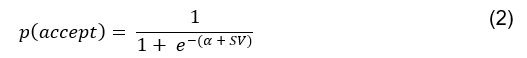
with for the predicted acceptance probability and 𝛼 for the intercept representing motivational tendency. A high motivational tendency means a subjects has a tendency, or bias, to accept rather than reject offers (Fig. 3D).

Our new figure (panels A-D in figure 3) visualizes the model. This demonstrates how the different model parameters come at play in the model (A), and how different values on each parameter affects the model (B-D).

- The early and late chronotype groups have significant differences in ages and gender. Additional supplementary analysis here may mitigate any concerns from readers.

The Reviewer is right to notice that our subsamples of early and late chronotypes differ significantly in age and gender, but it important to note that all our analyses comparing these two groups take this into account, statistically controlling for age and gender. We regret that this was previously only mentioned in the Methods section, so this information was not accessible where most relevant. To remedy this, we have amended the Results section as follows.

Lines 317 – 323:

“Bayesian GLMs, controlling for age and gender, predicting task parameters by time-of-day and chronotype showed effects of chronotype on reward sensitivity (i.e. those with a late chronotype had a higher reward sensitivity; M= 0.325, 95% HDI=[0.19,0.46]) and motivational tendency (higher in early chronotypes; M=-0.248, 95% HDI=[-0.37,-0.11]), as well as an interaction between chronotype and time-of-day on motivational tendency (M=0.309, 95% HDI=[0.15,0.48]).”

(2) Recommendations for improving the writing and presentation.

- I found the term 'overlapping' a little jarring. I think the authors use it to mean both neuropsychiatric symptoms and chronotypes affect task parameters, but they are are not tested to be 'separable', nor is an interaction tested. Perhaps being upfront about how interactions are not being tested here (in the introduction, and not waiting until the discussion) would give an opportunity to operationalize this term.

We agree with the Reviewer that our previously-used term “overlapping” was not ideal: it may have been misleading, and was not necessarily reflective of the nature of our findings. We now state explicitly that we are not testing an interaction between neuropsychiatric symptoms and chronotypes in our primary analyses. Additionally, following suggestions made by Reviewer 3, we ran new exploratory analyses to investigate how the effects of neuropsychiatric symptoms and circadian measures on motivational tendency relate to one another. These results in fact show that all three symptom measures have separable effects from circadian measures on motivational tendency. This supports the Reviewer’s view that ‘overlapping’ was entirely the wrong word—although it nevertheless shows the important contribution of circadian rhythm as well as neuropsychiatric symptoms in effort-based decision-making. We have changed the manuscript throughout to better describe this important, more accurate interpretation of our findings, including replacing the term “overlapping”. We changed the title from “Overlapping effects of neuropsychiatric symptoms and circadian rhythm on effort-based decision-making” to “Both neuropsychiatric symptoms and circadian rhythm alter effort-based decision-making”.

To clarify the intention of our primary analyses, we have added the following to the last paragraph of the introduction.

Lines 107 – 112:

“Next, we pre-registered a follow-up experiment to directly investigate how circadian preference interacts with time-of-day on motivational decision-making, using the same task and computational modelling approach. While this allows us to test how circadian effects on motivational decision-making compare to neuropsychiatric effects, we do not test for possible interactions between neuropsychiatric symptoms and chronobiology.”

We detail our new analyses in the Methods section as follows.

Lines 800 – 814:

“4.5.2 Differentiating between the effects of neuropsychiatric symptoms and circadian measures on motivational tendency

To investigate how the effects of neuropsychiatric symptoms on motivational tendency (2.3.1) relate to effects of chronotype and time-of-day on motivational tendency we conducted exploratory analyses. In the subsamples of participants with an early or late chronotype (including additionally collected data), we first ran Bayesian GLMs with neuropsychiatric questionnaire scores (SHAPS, DARS, AES respectively) predicting motivational tendency, controlling for age and gender. We next added an interaction term of chronotype and time-of-day into the GLMs, testing how this changes previously observed neuropsychiatric and circadian effects on motivational tendency. Finally, we conducted a model comparison using LOO, comparing between motivational tendency predicted by a neuropsychiatric questionnaire, motivational tendency predicted by chronotype and time-of-day, and motivational tendency predicted by a neuropsychiatric questionnaire and time-of-day (for each neuropsychiatric questionnaire, and controlling for age and gender).”

Results of the outlined analyses are reported in the Results section as follows.

Lines 356 – 383:

“2.5.2.1 Neuropsychiatric symptoms and circadian measures have separable effects on motivational tendency

Exploratory analyses testing for the effects of neuropsychiatric questionnaires on motivational tendency in the subsamples of early and late chronotypes confirmed the predictive value of the SHAPS (M=-0.24, 95% HDI=[-0.42,-0.06]), the DARS (M=-0.16, 95% HDI=[-0.31,-0.01]), and the AES (M=-0.18, 95% HDI=[-0.32,-0.02]) on motivational tendency.

For the SHAPS, we find that when adding the measures of chronotype and time-of-day back into the GLMs, the main effect of the SHAPS (M=-0.26, 95% HDI=[-0.43,-0.07]), the main effect of chronotype (M=-0.11, 95% HDI=[-0.22,-0.01]), and the interaction effect of chronotype and time-of-day (M=0.20, 95% HDI=[0.07,0.34]) on motivational tendency remain. Model comparison by LOOIC reveals motivational tendency is best predicted by the model including the SHAPS, chronotype and time-of-day as predictors, followed by the model including only the SHAPS. Note that this approach to model comparison penalizes models for increasing complexity.

Repeating these steps with the DARS, the main effect of the DARS is found numerically, but the 95% HDI just includes 0 (M=-0.15, 95% HDI=[-0.30,0.002]). The main effect of chronotype (M=-0.11, 95% HDI=[-0.21,-0.01]), and the interaction effect of chronotype and time-of-day (M=0.18, 95% HDI=[0.05,0.33]) on motivational tendency remain. Model comparison identifies the model including the DARS and circadian measures as the best model, followed by the model including only the DARS.

For the AES, the main effect of the AES is found (M=-0.19, 95% HDI=[-0.35,-0.04]). For the main effect of chronotype, the 95% narrowly includes 0 (M=-0.10, 95% HDI=[-0.21,0.002]), while the interaction effect of chronotype and time-of-day (M=0.20, 95% HDI=[0.07,0.34]) on motivational tendency remains. Model comparison identifies the model including the AES and circadian measures as the best model, followed by the model including only the AES.”

In addition to the title change, we edited our Discussion to discuss and reflect these new insights, including the following.

Lines 399 – 402:

“Various neuropsychiatric disorders are marked by disruptions in circadian rhythm, such as a late chronotype. However, research has rarely investigated how transdiagnostic mechanisms underlying neuropsychiatric conditions may relate to inter-individual differences in circadian rhythm.”

Lines 475 – 480:

“It is striking that the effects of neuropsychiatric symptoms on effort-based decision-making largely are paralleled by circadian effects on the same neurocomputational parameter. Exploratory analyses predicting motivational tendency by neuropsychiatric symptoms and circadian measures simultaneously indicate the effects go beyond recapitulating each other, but rather explain separable parts of the variance in motivational tendency.”

Lines 528 – 532:

“Our reported analyses investigating neuropsychiatric and circadian effects on effort-based decision-making simultaneously are exploratory, as our study design was not ideally set out to examine this. Further work is needed to disentangle separable effects of neuropsychiatric and circadian measures on effort-based decision-making.”

Lines 543 – 550:

“We demonstrate that neuropsychiatric effects on effort-based decision-making are paralleled by effects of circadian rhythm and time-of-day. Exploratory analyses suggest these effects account for separable parts of the variance in effort-based decision-making. It unlikely that effects of neuropsychiatric effects on effort-based decision-making reported here and in previous literature are a spurious result due to multicollinearity with chronotype. Yet, not accounting for chronotype and time of testing, which is the predominant practice in the field, could affect results.”

- A minor point, but it could be made clearer that many neurotransmitters have circadian rhythms (and not just dopamine).

We agree this should have been made clearer, and have added the following to the Introduction.

Lines 83 – 84:

“Bi-directional links between chronobiology and several neurotransmitter systems have been reported, including dopamine47.

(47) Kiehn, J.-T., Faltraco, F., Palm, D., Thome, J. & Oster, H. Circadian Clocks in the Regulation of Neurotransmitter Systems. Pharmacopsychiatry 56, 108–117 (2023).”

References

Hasselmann M, Gempe T, Schiøtt M, Nunes-Silva CG, Otte M, Beye M. 2008. Evidence for the evolutionary nascence of a novel sex determination pathway in honeybees. Nature 454:519–522.
Koch V, Nissen I, Schmitt BD, Beye M. 2014. Independent Evolutionary Origin of fem Paralogous Genes and Complementary Sex Determination in Hymenopteran Insects. PLOS ONE 9:e91883.
Matthey-Doret C, van der Kooi CJ, Jeffries DL, Bast J, Dennis AB, Vorburger C, Schwander T. 2019. Mapping of multiple complementary sex determination loci in a parasitoid wasp. Genome Biology and Evolution 11:2954–2962.
Miyakawa MO, Mikheyev AS. 2015. QTL mapping of sex determination loci supports an ancient pathway in ants and honey bees. PLOS Genetics 11:e1005656.
Pan Q, Darras H, Keller L. 2024. LncRNA gene ANTSR coordinates complementary sex determination in the Argentine ant. Science Advances 10:eadp1532.
Privman E, Wurm Y, Keller L. 2013. Duplication and concerted evolution in a master sex determiner under balancing selection. Proceedings of the Royal Society B: Biological Sciences 280:20122968.
Rabeling C, Kronauer DJC. 2012. Thelytokous parthenogenesis in eusocial Hymenoptera. Annual Review of Entomology 58:273–292.
Schmieder S, Colinet D, Poirié M. 2012. Tracing back the nascence of a new sex-determination pathway to the ancestor of bees and ants. Nature Communications 3:1–7.
Vorburger C. 2013. Thelytoky and Sex Determination in the Hymenoptera: Mutual Constraints. Sexual Development 8:50–58.
1. aportacion 3
Primero se define qué quieres investigar objetivo, y de ahí sale el título.
Si el título no coincide con lo que realmente se hizo, confunde al lector y resta credibilidad.
2. Aportacion 2 en la parte de que te exijan títulos supe cortos está bien hasta que te das cuenta de que terminas diciendo cualquier cosa. Es como cuando resumes una película y solo dices trata de algun problema.. pues sí pero no se entiende nada Mejor que sobre una palabra a que falte claridad.
1. Martínez-Pujalte, (2015)afirma que “los derechos fundamentales son propios de todo ser humano, que han sido constitucionalizados y están ligados con la misma dignidad, que según el aut
Cao, J., Willett, J. A., Dorris, D. M., & Meitzen, J. (2018). Sex DiMerences in Medium Spiny Neuron Excitability and Glutamatergic Synaptic Input: Heterogeneity Across Striatal Regions and Evidence for Estradiol-Dependent Sexual DiMerentiation. Front Endocrinol (Lausanne), 9, 173. https://doi.org/10.3389/fendo.2018.00173
Corbit, L. H., Muir, J. L., Balleine, B. W., & Balleine, B. W. (2001). The role of the nucleus accumbens in instrumental conditioning: Evidence of a functional dissociation between accumbens core and shell. J Neurosci, 21(9), 3251-3260. http://eutils.ncbi.nlm.nih.gov/entrez/eutils/elink.fcgi?dbfrom=pubmed&id=11312 310&retmode=ref&cmd=prlinks
Corbit, L. H., & Balleine, B. W. (2011). The general and outcome-specific forms of Pavlovian-instrumental transfer are diMerentially mediated by the nucleus accumbens core and shell. J Neurosci, 31(33), 11786-11794. https://doi.org/10.1523/JNEUROSCI.2711-11.2011
Laurent, V., Bertran-Gonzalez, J., Chieng, B. C., & Balleine, B. W. (2014). δ-Opioid and Dopaminergic Processes in Accumbens Shell Modulate the Cholinergic Control of Predictive Learning and Choice. J Neurosci, 34(4), 1358-1369. https://doi.org/10.1523/JNEUROSCI.4592-13.2014
Laurent, V., Leung, B., Maidment, N., & Balleine, B. W. (2012). μ- and δ-opioid-related processes in the accumbens core and shell diMerentially mediate the influence of reward-guided and stimulus-guided decisions on choice. J Neurosci, 32(5), 1875-1883. https://doi.org/10.1523/JNEUROSCI.4688-11.2012
Matamales, M., McGovern, A. E., Mi, J. D., Mazzone, S. B., Balleine, B. W., & BertranGonzalez, J. (2020). Local D2- to D1-neuron transmodulation updates goal-directed learning in the striatum. Science, 367(6477), 549-555. https://doi.org/10.1126/science.aaz5751
Parkes, S. L., Bradfield, L. A., & Balleine, B. W. (2015). Interaction of insular cortex and ventral striatum mediates the eMect of incentive memory on choice between goaldirected actions. J Neurosci, 35(16), 6464-6471. https://doi.org/10.1523/JNEUROSCI.4153-14.2015
Pettibone, J. R., Yu, J. Y., Derman, R. C., Faust, T. W., Hughes, E. D., Filipiak, W. E., Saunders, T. L., Ferrario, C. R., & Berke, J. D. (2019). Knock-In Rat Lines with Cre Recombinase at the Dopamine D1 and Adenosine 2a Receptor Loci. eNeuro, 6(5). https://doi.org/10.1523/ENEURO.0163-19.2019
Willett, J. A., Will, T., Hauser, C. A., Dorris, D. M., Cao, J., & Meitzen, J. (2016). No Evidence for Sex DiMerences in the Electrophysiological Properties and Excitatory Synaptic Input onto Nucleus Accumbens Shell Medium Spiny Neurons. eNeuro, 3(1), ENEURO.0147-15.2016. https://doi.org/10.1523/ENEURO.0147-15.2016
Alonso-Nanclares, L., Merino-Serrais, P., Gonzalez, S., & DeFelipe, J. (2013). Synaptic changes in the dentate gyrus of APP/PS1 transgenic mice revealed by electron microscopy. J Neuropathol Exp Neurol, 72(5), 386-395. doi:10.1097/NEN.0b013e31828d41ec
Bittner, T., Burgold, S., Dorostkar, M. M., Fuhrmann, M., Wegenast-Braun, B. M., Schmidt, B., . . . Herms, J. (2012). Amyloid plaque formation precedes dendritic spine loss. Acta Neuropathologica, 124(6), 797807. doi:10.1007/s00401-012-1047-8
Busche, M. A., Eichhoff, G., Adelsberger, H., Abramowski, D., Wiederhold, K. H., Haass, C., . . . Garaschuk, O. (2008). Clusters of hyperactive neurons near amyloid plaques in a mouse model of Alzheimer's disease. Science, 321(5896), 1686-1689. doi:10.1126/science.1162844
Grienberger, C., Rochefort, N. L., Adelsberger, H., Henning, H. A., Hill, D. N., Reichwald, J., . . . Konnerth, A. (2012). Staged decline of neuronal function in vivo in an animal model of Alzheimer's disease. Nat Commun, 3, 774. doi:10.1038/ncomms1783
Gureviciene, I., Ishchenko, I., Ziyatdinova, S., Jin, N., Lipponen, A., Gurevicius, K., & Tanila, H. (2019). Characterization of Epileptic Spiking Associated With Brain Amyloidosis in APP/PS1 Mice. Front Neurol, 10, 1151. doi:10.3389/fneur.2019.01151
Hijazi, S., Heistek, T. S., Scheltens, P., Neumann, U., Shimshek, D. R., Mansvelder, H. D., . . . van Kesteren, R. E. (2020a). Early restoration of parvalbumin interneuron activity prevents memory loss and network hyperexcitability in a mouse model of Alzheimer's disease. Mol Psychiatry, 25(12), 3380-3398. doi:10.1038/s41380-019-0483-4
Hijazi, S., Heistek, T. S., van der Loo, R., Mansvelder, H. D., Smit, A. B., & van Kesteren, R. E. (2020b). Hyperexcitable Parvalbumin Interneurons Render Hippocampal Circuitry Vulnerable to Amyloid Beta. iScience, 23(7), 101271. doi:10.1016/j.isci.2020.101271
Janota, C. S., Brites, D., Lemere, C. A., & Brito, M. A. (2015). Glio-vascular changes during ageing in wild-type and Alzheimer's disease-like APP/PS1 mice. Brain Res, 1620, 153-168. doi:10.1016/j.brainres.2015.04.056
Kater, M. S. J., Huffels, C. F. M., Oshima, T., Renckens, N. S., Middeldorp, J., Boddeke, E., . . . Verheijen, M. H. G. (2023). Prevention of microgliosis halts early memory loss in a mouse model of Alzheimer's disease. Brain Behav Immun, 107, 225-241. doi:10.1016/j.bbi.2022.10.009
Kim, H. Y., Kim, H. V., Jo, S., Lee, C. J., Choi, S. Y., Kim, D. J., & Kim, Y. (2015). EPPS rescues hippocampus-dependent cognitive deficits in APP/PS1 mice by disaggregation of amyloid-β oligomers and plaques. ature Communications, 6(1), 8997. doi:10.1038/ncomms9997
Olah, V. J., Goettemoeller, A. M., Rayaprolu, S., Dammer, E. B., Seyfried, N. T., Rangaraju, S., . . . Rowan, M. J. M. (2022). Biophysical Kv3 channel alterations dampen excitability of cortical PV interneurons and contribute to network hyperexcitability in early Alzheimer’s. Elife, 11, e75316. doi:10.7554/eLife.75316
Reyes-Marin, K. E., & Nuñez, A. (2017). Seizure susceptibility in the APP/PS1 mouse model of Alzheimer's disease and relationship with amyloid β plaques. Brain Res, 1677, 93-100. doi:10.1016/j.brainres.2017.09.026
Sohal, V. S., Zhang, F., Yizhar, O., & Deisseroth, K. (2009). Parvalbumin neurons and gamma rhythms enhance cortical circuit performance. Nature, 459(7247), 698-702. doi:10.1038/nature07991
van Heusden, F. C., van Nifterick, A. M., Souza, B. C., França, A. S. C., Nauta, I. M., Stam, C. J., . . . van Kesteren, R. E. (2023). Neurophysiological alterations in mice and humans carrying mutations in APP and PSEN1 genes. Alzheimers Res Ther, 15(1), 142. doi:10.1186/s13195-023-01287-6
Végh, M. J., Heldring, C. M., Kamphuis, W., Hijazi, S., Timmerman, A. J., Li, K. W., . . . van Kesteren, R. E. (2014). Reducing hippocampal extracellular matrix reverses early memory deficits in a mouse model of Alzheimer's disease. Acta Neuropathol Commun, 2, 76. doi:10.1186/s40478-014-0076-z
Verret, L., Mann, E. O., Hang, G. B., Barth, A. M., Cobos, I., Ho, K., . . . Palop, J. J. (2012). Inhibitory interneuron deficit links altered network activity and cognitive dysfunction in Alzheimer model. Cell, 149(3), 708-721. doi:10.1016/j.cell.2012.02.046
Xia, F., Richards, B. A., Tran, M. M., Josselyn, S. A., Takehara-Nishiuchi, K., & Frankland, P. W. (2017). Parvalbumin-positive interneurons mediate neocortical-hippocampal interactions that are necessary for memory consolidation. Elife, 6. doi:10.7554/eLife.27868
Zhang, W., Hao, J., Liu, R., Zhang, Z., Lei, G., Su, C., . . . Li, Z. (2011). Soluble Aβ levels correlate with cognitive deficits in the 12-month-old APPswe/PS1dE9 mouse model of Alzheimer's disease. Behavioural Brain Research, 222(2), 342-350. doi:https://doi.org/10.1016/j.bbr.2011.03.072
1. El texto critica la falta de perspectiva de género en las encuestas mexicanas sobre discriminación hacia migrantes, lo que genera una visión androcéntrica que invisibiliza a las mujeres. Destaca su valor al combinar una crítica metodológica con una reflexión feminista, mostrando que las encuestas también construyen realidad. No obstante, carece de evidencia empírica propia y no propone soluciones concretas para corregir el sesgo en el diseño de los cuestionarios.
2. La ceguera de género en las encuestas mexicanas sobre discriminación hacia a las personas inmigrantes
1. “al no incorporar una perspectiva de género en los cuestionarios, retratan una realidad equivocada.” pág. 181 Si bien la autora señala que la falta de incorporación de la perspectiva de género en los instrumentos de medición conduce a que los cuestionarios de las encuestas sobre migración y discriminación produzcan datos incompletos. Esto quiere decir, que, los resultados no reflejan diferencias sistemáticas entre hombres y mujeres migrantes, lo que a su vez limita la capacidad de conocer plenamente las dinámicas de discriminación basada en género dentro del fenómeno migratorio. En pocas palabras, si las encuestas no preguntan ¿Eres hombre o mujer migrante? o ¿Cómo afecta tu género tu experiencia migratoria?, entonces pasan por alto que las mujeres migrantes podrían estar viviendo discriminaciones distintas o adicionales. Es como si miráramos sólo la parte visible del iceberg y creyéramos que todo lo que importa está ahí arriba.
2. “no se considera la manera en que el género interseca con otras formas de desigualdad, como la nacionalidad o la clase social.” pág. 180 El texto resalta que la ceguera de género no sólo ignora las diferencias entre hombres y mujeres, sino que también desconoce la interseccionalidad. Es decir, el género se cruza con otros factores estructurales (como clase, etnicidad o estatus migratorio) que agravan las condiciones de vulnerabilidad. Su omisión impide comprender cómo las mujeres migrantes enfrentan formas múltiples y simultáneas de discriminación. Esto me parece clave, porque no todas las mujeres migrantes viven lo mismo, pues no es igual una mujer centroamericana pobre que una extranjera con más recursos. Ignorar esas diferencias es como decir que la discriminación afecta a todos igual, y eso borra las desigualdades que más pesan en la vida real.
3. “la de un país al que sólo llegan y por el que sólo transita una migración masculina.” pág. 180 Ahora bien, al describir el efecto de la “ceguera de género”, la autora observa que las encuestas reproducen un imaginario migratorio masculinizado, ya que, se asume implícitamente que la migración es mayoritariamente masculina. Esta visión sesgada impide reconocer la presencia, la situación y las necesidades específicas de las mujeres migrantes, reproduciendo una invisibilidad de género en los datos y, por ende, en las políticas públicas que podrían derivar de esos datos. Me hace pensar que muchas veces cuando escuchamos la palabra “los migrantes”, quizás pensamos automáticamente en hombres jóvenes. Pero, ¿Qué pasa con las mujeres que migran solas o en contexto familiar? Si los instrumentos no lo captan, es como si ni siquiera estuvieran consideradas. Y eso tiene consecuencias porque si no se mide, no se visibiliza, y si no se visibiliza, difícilmente se atiende.
(1) Biassoni R., Pessino A., Bottino C., Pende D., Moretta L., Moretta A. The murine homologue of the human NKp46, a triggering receptor involved in the induction of natural cytotoxicity. Eur J Immunol. 1999 Mar; 29(3).
(2) Glasner A., Roth Z., Varvak A., Miletic A., Isaacson B., Bar-On Y., Jonjić S., Khalaila I., Mandelboim O. Identification of putative novel O-glycosylations in the NK killer receptor Ncr1 essential for its activity. Cell Discov. 2015 Dec 22; 1:15036.
What are the inhibition results using F. nucleatum strains deficient in FadI?
The inhibition pattern observed in the F. nucleatum ΔFadI mutant was comparable to that of the wild-type strain (Author response image 6). When cultured under identical conditions and exposed to increasing concentrations of arginine (0, 5, and 10 mM), the F. nucleatum ΔFadI strain also demonstrated a dose-dependent reduction in binding to NKp46 and Ncr1.
Author response image 6. Arginine inhibition of NKp46-Ig and Ncr1-Ig binding in F. nucleatum ΔFadI. Histograms show NKp46-Ig (A, C) and Ncr1-Ig (B, D) binding to F. nucleatum ATCC10953 ΔFadI (A and B) and to F. nucleatum ATCC23726 ΔFadI (A and B) following exposure to 5 mM and 10 mM L-Arginine. Panels (E) and (F) display the mean fluorescence intensity (MFI) quantification corresponding to (A and B) and (C and D), respectively.
In Panel B, CEACAM1-Ig and RadD-deficient bacteria must be included as negative controls for binding specificity upon anti-NKp46 blocking.
We appreciate the request to include CEACAM1-Ig and RadD-deficient bacteria as negative controls for specificity under anti-NKp46 blocking. We don’t not think it is necessary since the 02 antibody is specific for NKp46, we used other anti0NKp46 antibodies that did not block the interaction and an irrelevant antibofy, we showed that arginine produced a dose-dependent reduction in NKp46/Ncr1 binding, consistent with an arginine-inhibitable RadD interaction already shown in our manuscript (Fig. 4A). The ΔRadD strains we used already demonstrate loss of NKp46/Ncr1 binding and loss of NK-boosting activity (Figs. 3, 5). Collectively, these data establish that NKp46/Ncr1 recognition of a high-molecular-weight ligand consistent with RadD is specific and functionally relevant.
Figure 5: Functional NK Activation and Tumor Killing
In Panels B and C, the key control condition (NK cells + anti-NKp46, without bacteria) is missing. This is needed to evaluate if NKp46 recognition is involved in tumor killing. The authors should explicitly test whether pre-incubation of NK cells with bacteria enhances their anti-tumor activity.
No significant difference in NK cell cytotoxicity was observed between untreated NK cells and NK cells incubated with anti-NKp46 antibody in the absence of bacteria. Therefore, the NK + anti-NKp46 (O2) group was included as an additional control alongside the other experimental conditions shown in Figures 5b and 5c, and is presented in Author response image 7 below.
Author response image 7. NK cytotoxicity against breast cancer cell lines. NK cell cytotoxicity against T47D (left) and MCF7 (right) breast cancer cell lines. This experiment follows the format of Figure 5b and 5c, with the addition of the NK cells + O2 antibody group. No significant differences were observed when values were normalized to NK cells alone.
Could bacteria induce stress signals in tumor cells that sensitize them to NK killing? This distinction is critical.
It remains unclear whether the bacteria induce stress-related signals in tumor cells that render them more susceptible to NK cell–mediated cytotoxicity.
(6) Figure 5D: Mechanism of Peripheral Activation
It is suggested that contact between bacteria and NK cells in the periphery leads to their activation. Can the authors confirm whether this pre-activation leads to enhanced killing of tumor targets, or if bacteria-tumor co-localization is required? The literature indicates that F. nucleatum localizes intracellularly within tumor cells. If so, how is RadD accessible to NKp46 on infiltrating NK cells?
We do not expect that pre-activation of NK cells with bacteria would enhance their tumor-killing capacity. In fact, when NK cells were co-incubated with bacteria, we occasionally observed NK cell death. Although F. nucleatum can reside intracellularly, bacterial entry requires prior adhesion to tumor cells. At this stage—before internalization—the bacteria are accessible for recognition and binding by NK cells.
(8) Figure 5E and In Vivo Relevance
Surprisingly, F. nucleatum infection is associated with increased tumor burden. Does this reflect an immunosuppressive effect? Are NK cells inhibited or exhausted in infected mice (TGIT, SIGLEC7...)? If NK cell activation leads to reduced tumor control in the infected context, the role of RadD-induced activation needs further explanation. RadD-deficient bacteria, which do not activate NK cells, result in even poorer tumor control. This paradox needs to be addressed: how can NK activation impair tumor control while its absence also reduces tumor control?
Siglec-7 lacks a direct orthologue in mice, and neither mouse TIGIT nor CEACAM1 bind F. nucleatum. The increased tumor burden observed in infected mice may therefore result from bacterial interference with immune cell infiltration and accumulation within the tumor microenvironment (Parhi, L., Alon-Maimon, T., Sol, A. et al. Breast cancer colonization by Fusobacterium nucleatum accelerates tumor growth and metastatic progression. Nat Commun 11, 3259 (2020)). Consequently, the NK cells that do reach the tumor site can recognize and kill F. nucleatum–bearing tumor cells through RadD–NKp46 interactions. In the absence of RadD, this recognition is impaired, leading to reduced NK-mediated cytotoxicity and increased tumor growth.
(9) NKp46-Deficient Mice: Inconsistencies
In Ncr1⁻/⁻ mice, infection with WT or RadD-deficient F. nucleatum has no impact on tumor burden. This suggests that NKp46 is dispensable in this context and casts doubt on the physiological relevance of the proposed mechanism. This contradiction should be discussed more thoroughly.
Ncr1 is also directly involved in mediating NK cell–dependent killing of tumor cells, even in the absence of bacterial infection. Therefore, in Ncr1-deficient mice, F. nucleatum has no additional effect on tumor progression (Glasner, A., Ghadially, H., Gur, C., Stanietsky, N., Tsukerman, P., Enk, J., Mandelboim, O. Recognition and prevention of tumor metastasis by the NK receptor NKp46/NCR1. J Immunol. 2012).
(1) Rosanova, M., Casali, A., Bellina, V., Resta, F., Mariotti, M., and Massimini, M. (2009). Natural frequencies of human corticothalamic circuits. J Neurosci 29, 7679-7685.
(2) Okazaki, Y.O., Nakagawa, Y., Mizuno, Y., Hanakawa, T., and Kitajo, K. (2021). Frequency- and Area-Specific Phase Entrainment of Intrinsic Cortical Oscillations by Repetitive Transcranial Magnetic Stimulation. Front Hum Neurosci 15, 608947.
References:

Bauknecht P, Jékely G. Large-Scale Combinatorial Deorphanization of Platynereis Neuropeptide GPCRs. Cell reports, 2015, 12(4), 684–693. doi:  10.1016/j.celrep.2015.06.052.
Beets I, Zels S, Vandewyer E, Demeulemeester J, et al. System-wide mapping of peptide-GPCR interactions in C. elegans. Cell reports, 2023, 42(9), 113058. doi: 10.1016/j.celrep.2023.113058.
Cardoso J C, Mc Shane J C, Li Z, et al. Revisiting the evolution of Family B1 GPCRs and ligands: Insights from mollusca. Molecular and cellular endocrinology, 2024, 586, 112192. doi: 10.1016/j.mce.2024.112192.
Gorn A H, Lin H Y, Yamin M, et al. Cloning, characterization, and expression of a human calcitonin receptor from an ovarian carcinoma cell line. The Journal of clinical investigation, 1992, 90(5), 1726–1735. doi: 10.1172/JCI116046.
Huang T, Su J, Wang X, et al. Functional Analysis and Tissue-Specific Expression of Calcitonin and CGRP with RAMP-Modulated Receptors CTR and CLR in Chickens. Animals: an open access journal from MDPI, 2024, 14(7), 1058. doi: 10.3390/ani14071058.
Johnson E C, Shafer O T, Trigg J S, et al. A novel diuretic hormone receptor in Drosophila: evidence for conservation of CGRP signaling. Journal of Experimental Biology, 2005, 208(7): 1239-1246. doi: 10.1242/jeb.01529.
McLatchie L M, Fraser N J, Main M J, et al. RAMPs regulate the transport and ligand specificity of the calcitonin-receptor-like receptor. Nature, 1998, 393(6683): 333-339. doi: 10.1038/30666.
Schwartz J, Réalis-Doyelle E, Dubos M P, et al. Characterization of an evolutionarily conserved calcitonin signaling system in a lophotrochozoan, the Pacific oyster (Crassostrea gigas). Journal of Experimental Biology, 2019, 222(13): jeb201319. doi: 10.1242/jeb.201319.
Sekiguchi T, Kuwasako K, Ogasawara M, et al. Evidence for conservation of the calcitonin superfamily and activity-regulating mechanisms in the basal chordate Branchiostoma floridae: insights into the molecular and functional evolution in chordates. Journal of Biological Chemistry, 2016, 291(5): 2345-2356. doi: 10.1074/jbc.M115.664003.
Expression of CT-like peptides was investigated both at transcript and protein level, but insight into the expression of the three peptide receptors is limited. This makes it difficult to understand the mechanism underlying the (different) functions of the two CT-like peptides in vivo. The authors identify differences in signal transduction cascades activated by each peptide, which might underpin distinct functions, but these differences were established only in heterologous cells.
Shafer, O. T., & Taghert, P. H. (2009). RNA-interference knockdown of Drosophila pigment dispersing factor in neuronal subsets: the anatomical basis of a neuropeptide's circadian functions. PloS one, 4(12), e8298. doi: 10.1371/journal.pone.0008298.
Van Sinay, E., Mirabeau, O., Depuydt, G., Van Hiel, M. B., Peymen, K., Watteyne, J., Zels, S., Schoofs, L., & Beets, I. (2017). Evolutionarily conserved TRH neuropeptide pathway regulates growth in Caenorhabditis elegans. Proceedings of the National Academy of Sciences of the United States of America, 114(20), E4065–E4074. doi: 10.1073/pnas.1617392114.
The new results following AjCT and AjPDFR2 knockdown are a welcome addition. While this additional evidence supports the claim that AjCT could mediate its effects via AjPDFR2, this evidence does not show that AjCT acts as an endogenous ligand for PDFR in vivo. In combination with the weak phylogenetic analyses, I would recommend the authors to key down their claims that they have functionally characterized a PDFR (in the title and text).
Thank you for your insightful comments and we do understand the reviewer’s concern.
Regarding “the weak phylogenetic analyses”, as highlighted above, we have produced a new phylogenetic tree (Fig 2, line 206) that provides strong bootstrap support for the clade comprising deuterostome and protostome PDF-type receptors. For this reason, it is our opinion that inclusion of “pigment-dispersing factor-type receptors” in the title of the paper is appropriate. The details of phylogenetic analysis method were added in line 727-739, and the updated phylogenetic tree has been incorporated into the revised manuscript (Figure 2, line 206). The description of new phylogenetic tree has also been modified accordingly in the revised manuscript (line 169-183). Besides, long-term knockdown of the AjCT precursor and AjPDFR2 both resulted in identical and significant growth defect phenotypes. And the observation of phenotypic overlap is widely accepted in genetic research as strong evidence for pathway association (Shafer and Taghert, 2009; Van Sinay et al., 2017). This high degree of phenotypic consistency, coupled with our in vitro finding that AjCT2 specifically activates AjPDFR2, strongly supports the conclusion that AjCT2 and AjPDFR2 function within the same signaling pathway in vivo, with AjPDFR2 serving as the key receptor functionally activated by AjCT2.
Since there is no formal logic defining the use of "type" vs "like" vs "related", I would encourage the authors to use one term (of their choice) to avoid unnecessary confusion. Or another possibility is that these relationships are defined at some point in the manuscript so that it becomes clear to the reader.
Thank you for the reviewer’s comments. The “CT-related peptides” has defined in the Introduction (line 54-58). As per your suggestion, we have now defined both “CT-type peptides” and “CT-like peptides” in the Introduction (line 76-79). “CT-type peptides” are characterized by an N-terminal disulphide bridge, whereas “CT-like peptides” (diuretic hormone 31 (DH31)-type peptides) lack this feature. Additionally, in accordance with the definitions, we have corrected these three descriptions in the revised manuscript (line 80, 83, 88 for “CT-type peptides”) to ensure consistent and accurate usage of these terms.
1. T designa el tratamiento y
T1: Aplicación foliar (por aspersión) de 1 % NPK, 1 % FeSO₄ y 1 % Zn en diferentes días del crecimiento (7, 15, 18, 22, 32 y 40 días). T2: Igual combinación de nutrientes que T1, pero aplicada por fertirrigación (disueltos en el agua de riego) en los mismos días. T3: Aplicación por fertirrigación de medio MS (Murashige y Skoog) al 5–10 % en distintas etapas del crecimiento (7, 15, 22 y 32 días). T4: Aplicación por fertirrigación de 1 % NPK y 1 % Zn en los días 7, 15, 22, 28, 32 y 45 del ciclo de cultivo. T5: Aplicación reducida de nutrientes por fertirrigación: 0,5 % NPK y 0,5 % Zn a los 7, 15, 18, 28 y 45 días. T6: Aplicación mínima y más eficiente por fertirrigación: 0,5 % NPK (a los 7–8 y 18 días), 0,5 % Zn (a los 15 días) y 1 % NPK (a los 28 días del crecimiento).
2. Las semillas secas se trataron con 100 ppm de GA₃ , 2 % de CaCl₂ , 1 % de KH₂PO₃ y 40 ppm de Na₂SeO₃ a una temperatura de 16 a 18 °C durante 20 h. Las semillas tratadas se lavaron 2 o 3 veces con agua destilada y se sembraron directamente en las bandejas de plántula para el siguiente ciclo de SpeedyPaddy.
Las semillas inmaduras fueron tratadas con una mezcla de hormonas y sales para romper la dormancia, estimular la germinación y fortalecer el embrión, permitiendo sembrar la siguiente generación en menos de un día.
3. cría rápida
Es un método usado en mejoramiento genético de cultivos para que las plantas crezcan, florezcan y produzcan semillas mucho más rápido. En lugar de esperar una sola cosecha al año, con la cría rápida se pueden lograr 4 o 5 generaciones de plantas en un mismo año.
1. The two distinct chromosomes referred to as X and Y arean important exception to the general pattern of homolo-gous chromosomes in human somatic cells.
XX chromosomes are homologous for females, XY chromosomes aren't homologous for males
Annotators
1. Las estrategias de comunicación deben estar diseñadas para incluir a todo el personal que forma parte de la empresa. Por ende, es reco-mendado utilizar canales digitales, intranets corporativas, chats internos, boletines de noticias a los que tengan acceso los empleados, pues este tipo de acciones permiten generar motivación y sentido de pertenencia en los trabajadores, lo cual repercute en la productividad de la industria
La inclusión es el pilar de una estrategia de comunicación efectiva, pues el incluir a todas las partes del personal, nos ayuda a reducir el ruido en la comunicación. Para lograr esto, así como lo expresa el texto es muy acertado el hacer uso de herramientas digitales modernas pues en este tiempo hay que empezar a digitalizarnos, asimismo esto nos puede garantizar que la información llegue a absolutamente todo el personal.
2. Es importante entender que los públicos con los que mantiene contacto la empresa son distintos; por ende, las estrategias deben ir direccionadas hacia ellos y cimentadas en el uso eficiente de los canales de comunicación apropiados, a fin de hacer llegar la propuesta de productos o servicios que ofertan de forma eficaz al público objetivo.
Considero que es esencial el recalcar esto, púes efectivamente cada empresa al tener diferentes giros, debe de efectuar diferentes estrategias, aunque todas deben de guiar hacia el mismo objetivo que es la buena comunicación bidireccional.
3. Cuando el sistema de comunicación empresarial es fluido y eficiente, se transmite un sentimiento de pertenencia y confianza en el personal, lo cual permite alcanzar el éxito sostenido de la organización, siempre que la comunicación sea oportuna, con información relevante y permanente (Oviedo, 2018). Neira (2018) asegura que la comunicación es uno de los elementos clave en las empresas modernas, puesto que facilita el intercambio de información entre el emisor y el receptor del mensaje y permite que exista un entendimiento mutuo entre las personas que forman parte de la comunicación, y, por tanto, que la información sea transmitida manteniendo el contexto original. Por su parte, Castro (2017) señala que la comunicación debe formar parte de la cultura organizacional y esto implica que todos los miembros de la empresa sean incluidos, a fin de mejorar la fluidez entre los diferentes niveles.
En esencia, este párrafo nos muestra como la comunicación interna es el pilar de una cultura empresarial exitosa. Cuando la información fluye de manera clara y constante, los empleados desarrollan un fuerte sentido de pertenencia y confianza en la organización, lo cual es fundamental para el éxito a largo plazo. No se trata solo de hablar, sino de evitar malentendidos; el objetivo es que el mensaje original se entienda perfectamente en todos los niveles, sin que se distorsione en el camino. Y efectivamente nos muestra como el tener un sistema de comunicación efectivo tiene múltiples ventajas.