10,000 Matching Annotations
  1. Dec 2025
    1. Note: This preprint has been reviewed by subject experts for Review Commons. Content has not been altered except for formatting.

      Learn more at Review Commons


      Referee #2

      Evidence, reproducibility and clarity

      Joint analysis of multiple modalities in single cells will provide a comprehensive view of cell fate states. In this manuscript, Bhardwaj et al developed a single-cell multi-omics assay, T-ChIC, to simultaneously capture histone modifications and full-length transcriptome and applied the method on early embryos of zebrafish. The authors observed a decoupled relationship between the chromatin modifications and gene expression at early developmental stages. The correlation becomes stronger as development proceeds, as genes are silenced by the cis-spreading of the repressive marker H3k27me3. Overall, the work is well performed, and the results are meaningful and interesting to readers in the epigenomic and embryonic development fields. There are some concerns before the manuscript is considered for publication.

      Major concerns:

      1. A major point of this study is to understand embryo development, especially gastrulation, with the power of scMulti-Omics assay. However, the current analysis didn't focus on deciphering the biology of gastrulation, i.e., lineage-specific pioneer factors that help to reform the chromatin landscape. The majority of the data analysis is based on the temporal dimension, but not the cell-type-specific dimension, which reduces the value of the single-cell assay.
      2. The cis-spreading of H3K27me3 with developmental time is interesting. Considering H3k27me3 could mark bivalent regions, especially in pluripotent cells, there must be some regions that have lost H3k27me3 signals during development. Therefore, it's confusing that the authors didn't find these regions (30% spreading, 70% stable). The authors should explain and discuss this issue.

      Minors:

      1. The authors cited two scMulti-omics studies in the introduction, but there have been lots of single-cell multi-omics studies published recently. The authors should cite and consider them.
      2. T-ChIC seems to have been presented in a previous paper (ref 15). Therefore, Fig. 1a is unnecessary to show.
      3. It's better to show the percentage of cell numbers (30% vs 70%) for each heatmap in Figure 2C.
      4. Please double-check the citation of Fig. S4C, which may not relate to the conclusion of signal differences between lineages.
      5. Figure 4C has not been cited or mentioned in the main text. Please check.

      Significance

      Strengths: This work utilized a new single-cell multi-omics method and generated abundant epigenomics and transcriptomics datasets for cells covering multiple key developmental stages of zebrafish. Limitations: The data analysis was superficial and mainly focused on the correspondence between the two modalities. The discussion of developmental biology was limited.

      Advance: The zebrafish single-cell datasets are valuable. The T-ChIC method is new and interesting.

      The audience will be specialized and from basic research fields, such as developmental biology, epigenomics, bioinformatics, etc.

      I'm more specialized in the direction of single-cell epigenomics, gene regulation, 3D genomics, etc.

    2. Note: This preprint has been reviewed by subject experts for Review Commons. Content has not been altered except for formatting.

      Learn more at Review Commons


      Referee #1

      Evidence, reproducibility and clarity

      The authors have a longstanding focus and reputation on single cell sequencing technology development and application. In this current study, the authors developed a novel single-cell multi-omic assay termed "T-ChIC" so that to jointly profile the histone modifications along with the full-length transcriptome from the same single cells, analyzed the dynamic relationship between chromatin state and gene expression during zebrafish development and cell fate determination. In general, the assay works well, the data look convincing and conclusions are beneficial to the community.

      There are several single-cell methodologies all claim to co-profile chromatin modifications and gene expression from the same individual cell, such as CoTECH, Paired-tag and others. Although T-ChIC employs pA-Mnase and IVT to obtain these modalities from single cells which are different, could the author provide some direct comparisons among all these technologies to see whether T-ChIC outperforms?

      In current study, T-ChIC profiled H3K27me3 and H3K4me1 modifications, these data look great. How about other histone modifications (eg H3K9me3 and H3K36me3) and transcription factors?

      T-ChIC can detect full length transcription from the same single cells, but in FigS3, the authors still used other published single cell transcriptomics to annotate the cell types, this seems unnecessary?

      Throughout the manuscript, the authors found some interesting dynamics between chromatin state and gene expression during embryogenesis, independent approaches should be used to validate these findings, such as IHC staining or RNA ISH?

      In Fig2 and FigS4, the authors showed H3K27me3 cis spreading during development, this looks really interesting. Is this zebrafish specific? H3K27me3 ChIP-seq or CutTag data from mouse and/or human embryos should be reanalyzed and used to compare. The authors could speculate some possible mechanisms to explain this spreading pattern?

      Significance

      The authors have a longstanding focus and reputation on single cell sequencing technology development and application. In this current study, the authors developed a novel single-cell multi-omic assay termed "T-ChIC" so that to jointly profile the histone modifications along with the full-length transcriptome from the same single cells, analyzed the dynamic relationship between chromatin state and gene expression during zebrafish development and cell fate determination. In general, the assay works well, the data look convincing and conclusions are beneficial to the community.

    1. <center>

      How the Rosetta Stone was discovered

      </center>

      <div style="background-color: silver; color: black; font-weight: bold;"> Nearly 2 000 years after the Rosetta stone decree was written, the French military engineer Pierre Francois Bouchard was repairing the defenses of an Arab Fort strengthening it against the ottoman Fleet that's expected to arrive within a short time. Only a year ago the French army had invaded Egypt and attempted to set up a colony but that increasingly looked doomed to failure as both the Ottomans and British were mustering to attack the French and the Army has to consistently battle internal revolts. </div>

      Discovery of the Rosetta Stone

      <div style="background-color: DarkCyan; color: white; font-weight: bold;"> During the repair work the engineers find the stone seemingly used as scrap construction material in an old wall. They immediately brought it to Bouchard's attention as they're supposed to do with any artifact. Seeing the script on the broken Stone Bouchard immediately realized the implications of this find as this inscription was in three different languages and it could be the key to finally deciphering Ancient Egyptian Hieroglyphics. so he sends out a message saying he's found a curious artifact near Rosetta the French name for Rasheed. </div>

      How Rosetta Stone was deciphered

      <div style="background-color: LightCyan; color: black; font-weight: bold;"> Bouchard sent out a message saying he's found a curious artifact near Rosetta, the French name for Rasheed. He then passed the stone to General Mano transferring it to his tent to be cleaned and the Greek to be translated while they dug in hopes of finding its missing pieces but then as the French army fought off an Ottoman landing at Abu kirbei Bouchard accompanied the 1700 pound Stone to the savants headquarters at Cairo. It arrived just in time for Napoleon to see it before he ditched the Expedition and sailed back to France. In doing so he left the savants with a deteriorating military situation alongside a Priceless but extremely heavy artifact that they had no way of getting back to France. </div>

      Note:The French Expedition also had an academic component of over 150 so-called savants - scientists, writers, linguists and other academics who had come along setting up a research institute in Cairo where they studied everything from local Wildlife to ancient artifacts.

      The deciphering of the Rosetta Stone

      Rosetta Stone changes hands from French to the British:

      It became soon obvious that the mysterious third language was not Syriac as originally thought but the Demotic mentioned in classical sources. At first they tried copying it by hand but it proved too intricate. Then they just smeared ink on the front and then pressed it with paper like it was a printing press. It worked ! All the while the French army hauled the stone around even to battlefields unwilling to leave it unguarded. Prints of the inscription had already reached Paris which was good because the Rosetta Stone could not be transported there.

      in 1801 General Menou, now in charge of the Expedition, signed a surrender agreement with the British and the Ottomans and one of the provisions was that all of the artifacts retrieved during the French expedition to Egypt were now Spoils of War and the personal property of King George III, especially the Rosetta Stone. In fact, the British were so pleased with its acquisition that they actually painted on the side "captured in Egypt by the British Army in 1801".

      Click Captured-by-British-Rosetta-Stone

      A year later when King George donated it to the British museum

    1. We also investigated how consistent the cell attention scores are across cross-validation splits, com-

      The paper notes that MultiMIL relies on batch-corrected embeddings to handle technical confounders, and that explicitly adding covariates like age/sex didn't improve performance. But beyond technical batch effects, patients often have heterogeneous biological states like unique inflammatory signatures, co-morbidities, disease subtypes, that are real biology but not common to the disease state. These could still be predictive in smaller cohorts without reflecting shared disease mechanisms. Does the attention mechanism have any inherent safeguard against overfitting to patient-specific biological features? In the stability analysis comparing embeddings (scVI versus scGPT), were there cases where the model consistently attended to features that were biologically real but unique to specific patients rather than the shared phenotype?

    1. Is Fast Charging Killing the Battery? A 2-Year Test on 40 Phones
      • Experiment Methodology: Researchers tested 40 phones over two years, completing 500 charge-discharge cycles using custom automation tools to compare the effects of different charging habits [00:01:11].
      • Fast Charging vs. Slow Charging: The study found that fast charging does not significantly harm battery health. After 500 cycles, the fast-charging iPhone group lost only 0.5% more capacity than the slow-charging group, while fast-charging Android phones actually showed slightly less wear than the slow-charging group [00:03:03].
      • The 30-80% Charging Habit: Maintaining a battery level between 30% and 80% reduced wear by 2.5% to 4% compared to full 0-100% cycles. While technically better, the researchers suggested the real-world benefit is limited compared to the effort [00:03:27].
      • Long-term Stability: Storing phones at 100% charge for a week showed no measurable change in capacity, reinforcing that battery degradation is a gradual, long-term process [00:04:13].
      • Battery Replacement Guidelines: Battery life begins to noticeably shorten when health drops to 85%, and the researchers recommend replacement when health reaches 80% to maintain a good user experience [00:05:01].
      • Performance & Throttling: Battery wear does not inherently slow down the phone's peak performance, but degraded batteries cause the system to throttle (slow down) earlier at low charge levels (e.g., at 11% instead of 5%) to prevent power failure [00:05:38].
      • Conclusion: The technical differences in battery wear from various charging methods are minimal. The best approach is to charge your phone conveniently and avoid trading "mental energy" for negligible battery gains [00:04:20].

    Tags

    Annotators

    URL

    1. It may be that what survives is a harder-to-automate version of online teaching, not a return to the days of Lotus Notes, but a new approach built around real instructor presence, with daily or biweekly check-ins.

      Again, how long have online instructors been building real instructor presence? This is NOT new.

    2. And when it comes to quizzes, even ones demanding written responses, AI can often outperform a rushed, underprepared human. It isn’t thinking, but it’s simulating the appearance of having thought. That’s often enough to get a B, even with an AI-aware instructor burying trip wires.

      There is no use for MC quizzes for anything other than voluntary self-assessment. They have been outmoded for a long time IMHO.

      Indeed, any forward thinking LMS really should have made other knowledge check or material exporation modalities available as native tools.

      Again, many thoughtful online teachers already found workarounds to create more pedagogically sound learning opportunities.

    3. These platforms weren’t designed to teach. They were designed to administer.

      Absolutely true!!! Anyone who thought that the LMS was doing the teaching was way off base in the first place! I agree that the LMS concept needs major work to keep up, but that is nothing new. And administration is also still a necessary function, so it is still servicable in that regard.

    4. It presents itself as modern, with its clickable modules and mobile-friendly interfaces, but the pedagogy behind it is stuck in another era.

      I'm not sure that I've ever thought of any LMS as modern and user-friendly, I've always thought of it as a barrier to get past and clunky tools to manage with the goal of delivering my course materials and pedagogical approach.

    1. Reviewer #3 (Public review):

      Summary:

      The authors propose a new version of idTracker.ai for animal tracking. Specifically, they apply contrastive learning to embed cropped images of animals into a feature space where clusters correspond to individual animal identities. By doing this, they address the requirement for so-called global fragments - segments of the video, in which all entities are visible/detected at the same time. In general, the new method reduces the long tracking times from the previous versions, while also increasing the average accuracy of assigning the identity labels.

      Strengths and weaknesses:

      The authors have reorganized and rewritten a substantial portion of their manuscript, which has improved the overall clarity and structure to some extent. In particular, omitting the different protocols enhanced readability. However, all technical details are now in appendix which is now referred to more frequently in the manuscript, which was already the case in the initial submission. These frequent references to the appendix - and even to appendices from previous versions - make it difficult to read and fully understand the method and the evaluations in detail. A more self-contained description of the method within the main text would be highly appreciated.

      Furthermore, the authors state that they changed their evaluation metric from accuracy to IDF1. However, throughout the manuscript they continue to refer to "accuracy" when evaluating and comparing results. It is unclear which accuracy metric was used or whether the authors are confusing the two metrics. This point needs clarification, as IDF1 is not an "accuracy" measure but rather an F1-score over identity assignments.

      The authors compare the speedups of the new version with those of the previous ones by taking the average. However, it appears that there are striking outliers in the tracking performance data (see Supplementary Table 1-4). Therefore, using the average may not be the most appropriate way to compare. The authors should consider using the median or providing more detailed statistics (e.g., boxplots) to better illustrate the distributions.

      The authors did not provide any conclusion or discussion section. Including a concise conclusion that summarizes the main findings and their implications would help to convey the message of the manuscript.

      The authors report an improvement in the mean accuracy across all benchmarks from 99.49% to 99.82% (with crossings). While this represents a slight improvement, the datasets used for benchmarking seem relatively simple and already largely "solved". Therefore, the impact of this work on the field may be limited. It would be more informative to evaluate the method on more challenging datasets that include frequent occlusions, crossings, or animals with similar appearances. The accuracy reported in the main text is "without crossings" - this seems like incomplete evaluation, especially that tracking objects that do not cross seems a straightforward task. Information is missing why crossings are a problem and are dealt with separately. There are several videos with a much lower tracking accuracy, explaining what the challenges of these videos are and why the method fails in such cases would help to understand the method's usability and weak points.

    2. Author response:

      The following is the authors’ response to the original reviews.

      Public Reviews:

      Reviewer #1 (Public review):

      Summary

      This is a strong paper that presents a clear advance in multi-animal tracking. The authors introduce an updated version of idtracker.ai that reframes identity assignment as a contrastive learning problem rather than a classification task requiring global fragments. This change leads to gains in speed and accuracy. The method eliminates a known bottleneck in the original system, and the benchmarking across species is comprehensive and well executed. I think the results are convincing and the work is significant.

      Strengths

      The main strengths are the conceptual shift from classification to representation learning, the clear performance gains, and the fact that the new version is more robust. Removing the need for global fragments makes the software more flexible in practice, and the accuracy and speed improvements are well demonstrated. The software appears thoughtfully implemented, with GUI updates and integration with pose estimators.

      Weaknesses

      I don't have any major criticisms, but I have identified a few points that should be addressed to improve the clarity and accuracy of the claims made in the paper.

      (1) The title begins with "New idtracker.ai," which may not age well and sounds more promotional than scientific. The strength of the work is the conceptual shift to contrastive representation learning, and it might be more helpful to emphasize that in the title rather than branding it as "new."

      We considered using “Contrastive idtracker.ai”. However, we thought that readers could then think that we believe they could use both the old idtracker.ai or this contrastive version. But we want to say that the new version is the one to use as it is better in both accuracy and tracking times. We think “New idtracker.ai” communicates better that this version is the version we recommend.

      (2) Several technical points regarding the comparison between TRex (a system evaluated in the paper) and idtracker.ai should be addressed to ensure the evaluation is fair and readers are fully informed.

      (2.1) Lines 158-160: The description of TRex as based on "Protocol 2 of idtracker.ai" overlooks several key additions in TRex, such as posture image normalization, tracklet subsampling, and the use of uniqueness feedback during training. These features are not acknowledged, and it's unclear whether TRex was properly configured - particularly regarding posture estimation, which appears to have been omitted but isn't discussed. Without knowing the actual parameters used to make comparisons, it's difficult to dassess how the method was evaluated.

      We added the information about the key additions of TRex in the section “The new idtracker.ai uses representation learning”, lines 153-157. Posture estimation in TRex was not explicitly used but neither disabled during the benchmark; we clarified this in the last paragraph of “Benchmark of accuracy and tracking time”, lines 492-495.

      (2.2) Lines 162-163: The paper implies that TRex gains speed by avoiding Protocol 3, but in practice, idtracker.ai also typically avoids using Protocol 3 due to its extremely long runtime. This part of the framing feels more like a rhetorical contrast than an informative one.

      We removed this, see new lines 153-157.

      (2.3) Lines 277-280: The contrastive loss function is written using the label l, but since it refers to a pair of images, it would be clearer and more precise to write it as l_{I,J}. This would help readers unfamiliar with contrastive learning understand the formulation more easily.

      We added this change in lines 613-620.

      (2.4) Lines 333-334: The manuscript states that TRex can fail to track certain videos, but this may be inaccurate depending on how the authors classify failures. TRex may return low uniqueness scores if training does not converge well, but this isn't equivalent to tracking failure. Moreover, the metric reported by TRex is uniqueness, not accuracy. Equating the two could mislead readers. If the authors did compare outputs to human-validated data, that should be stated more explicitly.

      We observed TRex crashing without outputting any trajectories on some occasions (Appendix 1—figure 1), and this is what we labeled as “failure”. These failures happened in the most difficult videos of our benchmark, that’s why we treated them the same way as idtracker.ai going to P3. We clarified this in new lines 464-469.

      The accuracy measured in our benchmark is not estimated but it is human-validated (see section Computation of tracking accuracy in Appendix 1). Both softwares report some quality estimators at the end of a tracking (“estimated accuracy” for idtracker.ai and "uniqueness” for TRex) but these were not used in the benchmark.

      (2.5) Lines 339-341: The evaluation approach defines a "successful run" and then sums the runtime across all attempts up to that point. If success is defined as simply producing any output, this may not reflect how experienced users actually interact with the software, where parameters are iteratively refined to improve quality.

      Yes, our benchmark was designed to be agnostic to the different experiences of the user. Also, our benchmark was designed for users that do not inspect the trajectories to choose parameters again not to leave room for potential subjectivity.

      (2.6) Lines 344-346: The simulation process involves sampling tracking parameters 10,000 times and selecting the first "successful" run. If parameter tuning is randomized rather than informed by expert knowledge, this could skew the results in favor of tools that require fewer or simpler adjustments. TRex relies on more tunable behavior, such as longer fragments improving training time, which this approach may not capture.

      We precisely used the TRex parameter track_max_speed to elongate fragments for optimal tracking. Rather than randomized parameter tuning, we defined the “valid range” for this parameter so that all values in it would produce a decent fragment structure. We used this procedure to avoid worsening those methods that use more parameters.

      (2.7) Line 354 onward: TRex was evaluated using two varying parameters (threshold and track_max_speed), while idtracker.ai used only one (intensity_threshold). With a fixed number of samples, this asymmetry could bias results against TRex. In addition, users typically set these parameters based on domain knowledge rather than random exploration.

      idtracker.ai and TRex have several parameters. Some of them have a single correct value (e.g. number of animals) or the default value that the system computes is already good (e.g. minimum blob size). For a second type of parameters, the system finds a value that is in general not as good, so users need to modify them. In general, users find that for this second type of parameter there is a valid interval of possible values, from which they need to choose a single value to run the system. idtracker.ai has intensity_threshold as the only parameter of this second type and TRex has two: threshold and track_max_speed. For these parameters, choosing one value or another within the valid interval can give different tracking results. Therefore, when we model a user that wants to run the system once except if it goes to P3 (idtracker.ai) or except if it crashes (TRex), it is these parameters we sample from within the valid interval to get a different value for each run of the system. We clarify this in lines 452-469 of the section “Benchmark of accuracy and tracking time”.

      Note that if we chose to simply run old idtracker.ai (v4 or v5) or TRex a single time, this would benefit the new idtracker.ai (v6). This is because old idtracker.ai can enter the very slow protocol 3 and TRex can fail to track. So running old idtracker.ai or TRex up to 5 times until old idtracker.ai does not use Protocol 3 and TRex does not fail is to make them as good as they can be with respect to the new idtracker.ai

      (2.8) Figure 2-figure supplement 3: The memory usage comparison lacks detail. It's unclear whether RAM or VRAM was measured, whether shared or compressed memory was included, or how memory was sampled. Since both tools dynamically adjust to system resources, the relevance of this comparison is questionable without more technical detail.

      We modified the text in the caption (new Figure 1-figure supplement 2) adding the kind of memory we measured (RAM) and how we measured it. We already have a disclaimer for this plot saying that memory management depends on the machine's available resources. We agree that this is a simple analysis of the usage of computer resources.

      (3) While the authors cite several key papers on contrastive learning, they do not use the introduction or discussion to effectively situate their approach within related fields where similar strategies have been widely adopted. For example, contrastive embedding methods form the backbone of modern facial recognition and other image similarity systems, where the goal is to map images into a latent space that separates identities or classes through clustering. This connection would help emphasize the conceptual strength of the approach and align the work with well-established applications. Similarly, there is a growing literature on animal re-identification (ReID), which often involves learning identity-preserving representations across time or appearance changes. Referencing these bodies of work would help readers connect the proposed method with adjacent areas using similar ideas, and show that the authors are aware of and building on this wider context.

      We have now added a new section in Appendix 3, “Differences with previous work in contrastive/metric learning” (lines 792-841) to include references to previous work and a description of what we do differently.

      (4) Some sections of the Results text (e.g., lines 48-74) read more like extended figure captions than part of the main narrative. They include detailed explanations of figure elements, sorting procedures, and video naming conventions that may be better placed in the actual figure captions or moved to supplementary notes. Streamlining this section in the main text would improve readability and help the central ideas stand out more clear

      Thank you for pointing this out. We have rewritten the Results, for example streamlining the old lines 48-74 (new lines 42-48)  by moving the comments about names, files and order of videos to the caption of Figure 1.

      Overall, though, this is a high-quality paper. The improvements to idtracker.ai are well justified and practically significant. Addressing the above comments will strengthen the work, particularly by clarifying the evaluation and comparisons.

      We thank the reviewer for the detailed suggestions. We believe we have taken all of them into consideration to improve the ms.

      Reviewer #2 (Public review):

      Summary:

      This work introduces a new version of the state-of-the-art idtracker.ai software for tracking multiple unmarked animals. The authors aimed to solve a critical limitation of their previous software, which relied on the existence of "global fragments" (video segments where all animals are simultaneously visible) to train an identification classifier network, in addition to addressing concerns with runtime speed. To do this, the authors have both re-implemented the backend of their software in PyTorch (in addition to numerous other performance optimizations) as well as moving from a supervised classification framework to a self-supervised, contrastive representation learning approach that no longer requires global fragments to function. By defining positive training pairs as different images from the same fragment and negative pairs as images from any two co-existing fragments, the system cleverly takes advantage of partial (but high-confidence) tracklets to learn a powerful representation of animal identity without direct human supervision. Their formulation of contrastive learning is carefully thought out and comprises a series of empirically validated design choices that are both creative and technically sound. This methodological advance is significant and directly leads to the software's major strengths, including exceptional performance improvements in speed and accuracy and a newfound robustness to occlusion (even in severe cases where no global fragments can be detected). Benchmark comparisons show the new software is, on average, 44 times faster (up to 440 times faster on difficult videos) while also achieving higher accuracy across a range of species and group sizes. This new version of idtracker.ai is shown to consistently outperform the closely related TRex software (Walter & Couzin, 2021\), which, together with the engineering innovations and usability enhancements (e.g., outputs convenient for downstream pose estimation), positions this tool as an advancement on the state-of-the-art for multi-animal tracking, especially for collective behavior studies.

      Despite these advances, we note a number of weaknesses and limitations that are not well addressed in the present version of this paper:

      Weaknesses

      (1) The contrastive representation learning formulation. Contrastive representation learning using deep neural networks has long been used for problems in the multi-object tracking domain, popularized through ReID approaches like DML (Yi et al., 2014\) and DeepReID (Li et al., 2014). More recently, contrastive learning has become more popular as an approach for scalable self-supervised representation learning for open-ended vision tasks, as exemplified by approaches like SimCLR (Chen et al., 2020), SimSiam (Chen et al., 2020\), and MAE (He et al., 2021\) and instantiated in foundation models for image embedding like DINOv2 (Oquab et al., 2023). Given their prevalence, it is useful to contrast the formulation of contrastive learning described here relative to these widely adopted approaches (and why this reviewer feels it is appropriate):

      (1.1) No rotations or other image augmentations are performed to generate positive examples. These are not necessary with this approach since the pairs are sampled from heuristically tracked fragments (which produces sufficient training data, though see weaknesses discussed below) and the crops are pre-aligned egocentrically (mitigating the need for rotational invariance).

      (1.2) There is no projection head in the architecture, like in SimCLR. Since classification/clustering is the only task that the system is intended to solve, the more general "nuisance" image features that this architectural detail normally affords are not necessary here.

      (1.3) There is no stop gradient operator like in BYOL (Grill et al., 2020\) or SimSiam. Since the heuristic tracking implicitly produces plenty of negative pairs from the fragments, there is no need to prevent representational collapse due to class asymmetry. Some care is still needed, but the authors address this well through a pair sampling strategy (discussed below).

      (1.4) Euclidean distance is used as the distance metric in the loss rather than cosine similarity as in most contrastive learning works. While cosine similarity coupled with L2-normalized unit hypersphere embeddings has proven to be a successful recipe to deal with the curse of dimensionality (with the added benefit of bounded distance limits), the authors address this through a cleverly constructed loss function that essentially allows direct control over the intra- and inter-cluster distance (D\_pos and D\_neg). This is a clever formulation that aligns well with the use of K-means for the downstream assignment step.

      No concerns here, just clarifications for readers who dig into the review. Referencing the above literature would enhance the presentation of the paper to align with the broader computer vision literature.

      Thank you for this detailed comparison. We have now added a new section in Appendix 3, “Differences with previous work in contrastive/metric learning” (lines 792-841) to include references to previous work and a description of what we do differently, including the points raised by the reviewer.

      (2) Network architecture for image feature extraction backbone. As most of the computations that drive up processing time happen in the network backbone, the authors explored a variety of architectures to assess speed, accuracy, and memory requirements. They land on ResNet18 due to its empirically determined performance. While the experiments that support this choice are solid, the rationale behind the architecture selection is somewhat weak. The authors state that: "We tested 23 networks from 8 different families of state-of-the-art convolutional neural network architectures, selected for their compatibility with consumer-grade GPUs and ability to handle small input images (20 × 20 to 100 × 100 pixels) typical in collective animal behavior videos."

      (2.1) Most modern architectures have variants that are compatible with consumer-grade GPUs. This is true of, for example, HRNet (Wang et al., 2019), ViT (Dosovitskiy et al., 2020), SwinT (Liu et al., 2021), or ConvNeXt (Liu et al., 2022), all of which report single GPU training and fast runtime speeds through lightweight configuration or subsequent variants, e.g., MobileViT (Mehta et al., 2021). The authors may consider revising that statement or providing additional support for that claim (e.g., empirical experiments) given that these have been reported to outperform ResNet18 across tasks.

      Following the recommendation of the reviewer, we tested the architectures SwinT, ConvNeXt and ViT. We found out that none of them outperformed ResNet18 since they all showed a slower learning curve. This would result in higher tracking times. These tests are now included in the section “Network architecture” (lines 550-611).

      (2.2) The compatibility of different architectures with small image sizes is configurable. Most convolutional architectures can be readily adapted to work with smaller image sizes, including 20x20 crops. With their default configuration, they lose feature map resolution through repeated pooling and downsampling steps, but this can be readily mitigated by swapping out standard convolutions with dilated convolutions and/or by setting the stride of pooling layers to 1, preserving feature map resolution across blocks. While these are fairly straightforward modifications (and are even compatible with using pretrained weights), an even more trivial approach is to pad and/or resize the crops to the default image size, which is likely to improve accuracy at a possibly minimal memory and runtime cost. These techniques may even improve the performance with the architectures that the authors did test out.

      The only two tested architectures that require a minimum image size are AlexNet and DenseNet. DenseNet proved to underperform ResNet18 in the videos where the images are sufficiently large. We have tested AlexNet with padded images to see that it also performs worse than ResNet18 (see Appendix 3—figure 1).

      We also tested the initialization of ResNet18 with pre-trained weights from ImageNet (in Appendix 3—figure 2) and it proved to bring no benefit to the training speed (added in lines 591-592).

      (2.3) The authors do not report whether the architecture experiments were done with pretrained or randomly initialized weights.

      We adapted the text to make it clear that the networks are always randomly initialized (lines 591-592, lines 608-609 and the captions of Appendix 3—figure 1 and 2).

      (2.4) The authors do not report some details about their ResNet18 design, specifically whether a global pooling layer is used and whether the output fully connected layer has any activation function. Additionally, they do not report the version of ResNet18 employed here, namely, whether the BatchNorm and ReLU are applied after (v1) or before (v2) the conv layers in the residual path.

      We use ResNet18 v1 with no activation function nor bias in its last layer (this has been clarified in the lines 606-608). Also, by design, ResNet has a global average pool right before the last fully connected layer which we did not remove. In response to the reviewer, Resnet18 v2 was tested and its performance is the same as that of v1 (see Appendix 3—figure 1 and lines 590-591).

      (3) Pair sampling strategy. The authors devised a clever approach for sampling positive and negative pairs that is tailored to the nature of the formulation. First, since the positive and negative labels are derived from the co-existence of pretracked fragments, selection has to be done at the level of fragments rather than individual images. This would not be the case if one of the newer approaches for contrastive learning were employed, but it serves as a strength here (assuming that fragment generation/first pass heuristic tracking is achievable and reliable in the dataset). Second, a clever weighted sampling scheme assigns sampling weights to the fragments that are designed to balance "exploration and exploitation". They weigh samples both by fragment length and by the loss associated with that fragment to bias towards different and more difficult examples.

      (3.1) The formulation described here resembles and uses elements of online hard example mining (Shrivastava et al., 2016), hard negative sampling (Robinson et al., 2020\), and curriculum learning more broadly. The authors may consider referencing this literature (particularly Robinson et al., 2020\) for inspiration and to inform the interpretation of the current empirical results on positive/negative balancing.

      Following this recommendation, we added references of hard negative mining in the new section “Differences with previous work in contrastive/metric learning”, lines 792-841. Regarding curriculum learning, even though in spirit it might have parallels with our sampling method in the sense that there is a guided training of the network, we believe the approach is more similar to an exploration-exploitation paradigm.

      (4) Speed and accuracy improvements. The authors report considerable improvements in speed and accuracy of the new idTracker (v6) over the original idTracker (v4?) and TRex. It's a bit unclear, however, which of these are attributable to the engineering optimizations (v5?) versus the representation learning formulation.

      (4.1) Why is there an improvement in accuracy in idTracker v5 (L77-81)? This is described as a port to PyTorch and improvements largely related to the memory and data loading efficiency. This is particularly notable given that the progression went from 97.52% (v4; original) to 99.58% (v5; engineering enhancements) to 99.92% (v6; representation learning), i.e., most of the new improvement in accuracy owes to the "optimizations" which are not the central emphasis of the systematic evaluations reported in this paper.

      V5 was a two year-effort designed to improve time efficiency of v4. It was also a surprise to us that accuracy was higher, but that likely comes from the fact that the substituted code from v4 contained some small bug/s. The improvements in v5 are retained in v6 (contrastive learning) and v6 has higher accuracy and shorter tracking times. The difference in v6 for this extra accuracy and shorter tracking times is contrastive learning.

      (4.2) What about the speed improvements? Relative to the original (v4), the authors report average speed-ups of 13.6x in v5 and 44x in v6. Presumably, the drastic speed-up in v6 comes from a lower Protocol 2 failure rate, but v6 is not evaluated in Figure 2 - figure supplement 2.

      Idtracker.ai v5 runs an optimized Protocol 2 and, sometimes, the Protocol 3. But v6 doesn’t run either of them. While P2 is still present in v6 as a fallback protocol when contrastive fails, in our v6 benchmark P2 was never needed. So the v6 speedup comes from replacing both P2 and P3 with the contrastive algorithm.

      (5) Robustness to occlusion. A major innovation enabled by the contrastive representation learning approach is the ability to tolerate the absence of a global fragment (contiguous frames where all animals are visible) by requiring only co-existing pairs of fragments owing to the paired sampling formulation. While this removes a major limitation of the previous versions of idtracker.ai, its evaluation could be strengthened. The authors describe an ablation experiment where an arc of the arena is masked out to assess the accuracy under artificially difficult conditions. They find that the v6 works robustly up to significant proportions of occlusions, even when doing so eliminates global fragments.

      (5.1) The experiment setup needs to be more carefully described.

      (5.1.1) What does the masking procedure entail? Are the pixels masked out in the original video or are detections removed after segmentation and first pass tracking is done?

      The mask is defined as a region of interest in the software. This means that it is applied at the segmentation step where the video frame is converted to a foreground-background binary image. The region of interest is applied here, converting to background all pixels not inside of it. We clarified this in the newly added section Occlusion tests, lines 240-244.

      (5.1.2) What happens at the boundary of the mask? (Partial segmentation masks would throw off the centroids, and doing it after original segmentation does not realistically model the conditions of entering an occlusion area.)

      Animals at the boundaries of the mask are partially detected. This can change the location of their detected centroid. That’s why, when computing the ground-truth accuracy for these videos, only the groundtruth centroids that were at minimum 15 pixels further from the mask were considered. We clarified this in the newly added section Occlusion tests, lines 248-251.

      (5.1.3) Are fragments still linked for animals that enter and then exit the mask area?

      No artificial fragment linking was added in these videos. Detected fragments are linked the usual way. If one animal hides into the mask, the animal disappears so the fragment breaks.  We clarified this in the newly added section Occlusion tests, lines 245-247.

      (5.1.4) How is the evaluation done? Is it computed with or without the masked region detections?

      The groundtruth used to validate these videos contains the positions of all animals at all times. But only the positions outside the mask at each frame were considered to compute the tracking accuracy. We clarified this in the newly added section Occlusion tests, lines 248-251.

      (5.2) The circular masking is perhaps not the most appropriate for the mouse data, which is collected in a rectangular arena.

      We wanted to show the same proof of concept in different videos. For that reason, we used to cover the arena parametrized by an angle. In the rectangular arena the circular masking uses an external circle, so it is covering the rectangle parametrized by an angle.

      (5.3) The number of co-existing fragments, which seems to be the main determinant of performance that the authors derive from this experiment, should be reported for these experiments. In particular, a "number of co-existing fragments" vs accuracy plot would support the use of the 0.25(N-1) heuristic and would be especially informative for users seeking to optimize experimental and cage design. Additionally, the number of co-existing fragments can be artificially reduced in other ways other than a fixed occlusion, including random dropout, which would disambiguate it from potential allocentric positional confounds (particularly relevant in arenas where egocentric pose is correlated with allocentric position).

      We included the requested analysis about the fragment connectivity in Figure 3-figure supplement 1. We agree that there can be additional ways of reducing co-existing fragments, but we think the occlusion tests have the additional value that there are many real experiments similar to this test.

      (6) Robustness to imaging conditions. The authors state that "the new idtracker.ai can work well with lower resolutions, blur and video compression, and with inhomogeneous light (Figure 2 - figure supplement 4)." (L156). Despite this claim, there are no speed or accuracy results reported for the artificially corrupted data, only examples of these image manipulations in the supplementary figure.

      We added this information in the same image, new Figure 1 - figure supplement 3.

      (7) Robustness across longitudinal or multi-session experiments. The authors reference idmatcher.ai as a compatible tool for this use case (matching identities across sessions or long-term monitoring across chunked videos), however, no performance data is presented to support its usage. This is relevant as the innovations described here may interact with this setting. While deep metric learning and contrastive learning for ReID were originally motivated by these types of problems (especially individuals leaving and entering the FOV), it is not clear that the current formulation is ideally suited for this use case. Namely, the design decisions described in point 1 of this review are at times at odds with the idea of learning generalizable representations owing to the feature extractor backbone (less scalable), low-dimensional embedding size (less representational capacity), and Euclidean distance metric without hypersphere embedding (possible sensitivity to drift). It's possible that data to support point 6 can mitigate these concerns through empirical results on variations in illumination, but a stronger experiment would be to artificially split up a longer video into shorter segments and evaluate how generalizable and stable the representations learned in one segment are across contiguous ("longitudinal") or discontiguous ("multi-session") segments.

      We have now added a test to prove the reliability of idmatcher.ai in v6. In this test, 14 videos are taken from the benchmark and split in two non-overlapping parts (with a 200 frames gap in between). idmatcher.ai is run between the two parts presenting a 100% accuracy identity matching across all of them (see section “Validity of idmatcher.ai in the new idtracker.ai”, lines 969-1008).

      We thank the reviewer for the detailed suggestions. We believe we have taken all of them into consideration to improve the ms.

      Reviewer #3 (Public review):

      Summary

      The authors propose a new version of idTracker.ai for animal tracking. Specifically, they apply contrastive learning to embed cropped images of animals into a feature space where clusters correspond to individual animal identities.

      Strengths

      By doing this, the new software alleviates the requirement for so-called global fragments - segments of the video, in which all entities are visible/detected at the same time - which was necessary in the previous version of the method. In general, the new method reduces the tracking time compared to the previous versions, while also increasing the average accuracy of assigning the identity labels.

      Weaknesses

      The general impression of the paper is that, in its current form, it is difficult to disentangle the old from the new method and understand the method in detail. The manuscript would benefit from a major reorganization and rewriting of its parts. There are also certain concerns about the accuracy metric and reducing the computational time.

      We have made the following modifications in the presentation:

      (1) We have added section tiles to the main text so it is clearer what tracking system we are referring to. For example, we now have sections “Limitation of the original idtracker.ai”, “Optimizing idtracker.ai without changes in the learning method” and “The new idtracker.ai uses representation learning”.

      (2) We have completely rewritten all the text of the ms until we start with contrastive learning. Old L20-89 is now L20-L66, much shorter and easier to read.

      (3) We have rewritten the first 3 paragraphs in the section “The new idtracker.ai uses representation learning” (lines 68-92).

      (4) We now expanded Appendix 3 to discuss the details of our approach  (lines 539-897).  It discusses in detail the steps of the algorithm, the network architecture, the loss function, the sampling strategy, the clustering and identity assignment, and the stopping criteria in training

      (5) To cite previous work in detail and explain what we do differently, we have now added in Appendix 3 the new section “Differences with previous work in contrastive/metric learning” (lines 792-841).

      Regarding accuracy metrics, we have replaced our accuracy metric with the standard metric IDF1. IDF1 is the standard metric that is applied to systems in which the goal is to maintain consistent identities across time. See also the section in Appendix 1 "Computation of tracking accuracy” (lines 414-436) explaining IDF1 and why this is an appropriate metric for our goal.

      Using IDF1 we obtain slightly higher accuracies for the idtracker.ai systems. This is the comparison of mean accuracy over all our benchmark for our previous accuracy score and the new one for the full trajectories:

      v4:   97.42% -> 98.24%

      v5:   99.41% -> 99.49%

      v6:   99.74% -> 99.82%

      trex: 97.89% -> 97.89%

      We thank the reviewer for the suggestions about presentation and about the use of more standard metrics.

      Recommendations for the authors:

      Reviewer #2 (Recommendations for the authors):

      (1) Figure 1a: A graphical legend inset would make it more readable since there are multiple colors, line styles, and connecting lines to parse out.

      Following this recommendation, we added a graphical legend in the old Figure 1 (new Figure 2).

      (2) L46: "have images" → "has images".

      We applied this correction. Line 35.

      (3) L52: "videos start with a letter for the species (z,**f**,m)", but "d" is used for fly videos.

      We applied this correction in the caption of Figure 1.

      (4) L62: "with Protocol 3 a two-step process" → "with Protocol 3 being a two-step process".

      We rewrote this paragraph without mentioning Protocol 3, lines 37-41.

      (5) L82-89: This is the main statement of the problems that are being addressed here (speed and relaxing the need for global fragments). This could be moved up, emphasized, and made clearer without the long preamble and results on the engineering optimizations in v5. This lack of linearity in the narrative is also evident in the fact that after Figure 1a is cited, inline citations skip to Figure 2 before returning to Figure 1 once the contrastive learning is introduced.

      We have rewritten all the text until the contrastive learning, (old lines 20-89 are now lines 20-66). The text is shorter, more linear and easier to read.

      (6) L114: "pairs until the distance D_{pos}" → "pairs until the distance approximates D_{pos}".

      We rewrote as “ pairs until the distance 𝐷pos (or 𝐷neg) is reached” in line 107.

      (7) L570: Missing a right parenthesis in the equation.

      We no longer have this equation in the ms.

      (8) L705: "In order to identify fragments we, not only need" → "In order to identify fragments, we not only need".

      We applied this correction, Line 775.

      (9) L819: "probably distribution" → "probability distribution".

      We applied this correction, Line 776.

      (10) L833: "produced the best decrease the time required" → "produced the best decrease of the time required".

      We applied this correction, Line 746.

      Reviewer #3 (Recommendations for the authors):

      (1) We recommend rewriting and restructuring the manuscript. The paper includes a detailed explanation of the previous approaches (idTracker and idTracker.ai) and their limitations. In contrast, the description of the proposed method is short and unstructured, which makes it difficult to distinguish between the old and new methods as well as to understand the proposed method in general. Here are a few examples illustrating the problem. 

      (1.1) Only in line 90 do the authors start to describe the work done in this manuscript. The previous 3 pages list limitations of the original method.

      We have now divided the main text into sections, so it is clearer what is the previous method (“Limitation of the original idtracker.ai”, lines 28-51), the new optimization we did of this method (“Optimizing idtracker.ai without changes in the learning method”, lines 52-66) and the new contrastive approach that also includes the optimizations (“The new idtracker.ai uses representation learning”, lines 66-164). Also, the new text has now been streamlined until the contrastive section, following your suggestion. You can see that in the new writing the three sections are 25 , 15 and 99 lines. The more detailed section is the new system, the other two are needed as reference, to describe which problem we are solving and the extra new optimizations.  

      (1.2) The new method does not have a distinct name, and it is hard to follow which idtracker.ai is a specific part of the text referring to. Not naming the new method makes it difficult to understand.

      We use the name new idtracker.ai (v6) so it becomes the current default version. v5 is now obsolete, as well as v4. And from the point of view of the end user, no new name is needed since v6 is just an evolution of the same software they have been using. Also, we added sections in the main text to clarify the ideas in there and indicate the version of idtracker.ai we are referring to.

      (1.3) There are "Protocol 2" and "Protocol 3" mixed with various versions of the software scattered throughout the text, which makes it hard to follow. There should be some systematic naming of approaches and a listing of results introduced.

      Following this recommendation we no longer talk about the specific protocols of the old version of idtracker.ai in the main text. We rewritten the explanation of these versions in a more clear and straightforward way, lines 29-36.

      (2) To this end, the authors leave some important concepts either underexplained or only referenced indirectly via prior work. For example, the explanation of how the fragments are created (line 15) is only explained by the "video structure" and the algorithm that is responsible for resolving the identities during crossings is not detailed (see lines 46-47, 149-150). Including summaries of these elements would improve the paper's clarity and accessibility.

      We listed the specific sections from our previous publication where the reader can find information about the entire tracking pipeline (lines 539-549). This way, we keep the ms clear and focused on the new identification algorithm while indicating where to find such information.

      (3) Accuracy metrics are not clear. In line 319, the authors define it as based on "proportion of errors in the trajectory". This proportion is not explained. How is the error calculated if a trajectory is lost or there are identity swaps? Multi-object tracking has a range of accuracy metrics that account for such events but none of those are used by the authors. Estimating metrics that are common for MOT literature, for example, IDF1, MOTA, and MOTP, would allow for better method performance understanding and comparison.

      In the new ms, we replaced our accuracy metric with the standard metric IDF1. IDF1 is the standard metric that is applied to systems in which the goal is to maintain consistent identities across time. See also the section in Appendix 1 "Computation of tracking accuracy” explaining why IDF1 and not MOTA or MOTP is the adequate metric for a system that wants to give correct tracking by identification in time. See lines 416-436.

      Using IDF1 we obtain slightly higher accuracies for the idtracker.ai systems. This is the comparison of mean accuracy four our previous accuracy and the new one for the full trajectories:

      v4:   97.42% -> 98.24%

      v5:   99.41% -> 99.49%

      v6:   99.74% -> 99.82%

      trex: 97.89% -> 97.89%

      (4) Additionally, the authors distinguish between tracking with and without crossings, but do not provide statistics on the frequency of crossings per video. It is also unclear how the crossings are considered for the final output. Including information such as the frame rate of the videos would help to better understand the temporal resolution and the differences between consecutive frames of the videos.

      We added this information in the Appendix 1 “Benchmark of accuracy and tracking time”, lines 445-451. The framerate in our benchmark videos goes from 25 to 60 fps (average of 37 fps). On average 2.6% of the blobs are crossings (1.1% for zebrafish 0.7% for drosophila 9.4% for mice).

      (5) In the description of the dataset used for evaluation (lines 349-365), the authors describe the random sampling of parameter values for each tracking run. However, it is unclear whether the same values were used across methods. Without this clarification, comparisons between the proposed method, older versions, and TRex might be biased due to lucky parameter combinations. In addition, the ranges from which the values were randomly sampled were also not described.

      Only one parameter is shared between idtracker.ai and TRex: intensity_threshold (in idtracker.ai) and threshold (in TRex). Both are conceptually equivalent but differ in their numerical values since they affect different algorithms. V4, v5, and TRex each required the same process of independent expert visual inspection of the segmentation to select the valid value range. Since versions 5 and 6 use exactly the same segmentation algorithm, they share the same parameter ranges.

      All the ranges of valid values used in our benchmark are public here https://drive.google.com/drive/folders/1tFxdtFUudl02ICS99vYKrZLeF28TiYpZ as stated in the section “Data availability”, lines 227-228.

      (6) Lines 122-123, Figure 1c. "batches" - is an imprecise metric of training time as there is no information about the batch size.

      We clarified the Figure caption, new Figure 2c.

      (7) Line 145 - "we run some steps... For example..." leaves the method description somewhat unclear. It would help if you could provide more details about how the assignments are carried out and which metrics are being used.

      Following this recommendation, we listed the specific sections from our previous publication where the reader can find information about the entire tracking pipeline (lines 539-549). This way, we keep the ms clear and focused on the new identification algorithm while indicating where to find such information.

      (8) Figure 3. How is tracking accuracy assessed with occlusions? Are the individuals correctly recognized when they reappear from the occluded area?

      The groundtruth for this video contains the positions of all animals at all times. Only the groundtruth points inside the region of interest are taken into account when computing the accuracy. When the tracking reaches high accuracy, it means that animals are successfully relabeled every time they enter the non-masked region. Note that this software works all the time by identification of animals, so crossings and occlusion are treated the same way. What is new here is that the occlusions are so large that there are no global fragments. We clarified this in the new section “Occlusion tests” in Methods, lines 239-251.

      (9) Lines 185-187 this part of the sentence is not clear.

      We rewrote this part in a clearer way, lines 180-182.

      (10) The authors also highlight the improved runtime performance. However, they do not provide a detailed breakdown of the time spent on each component of the tracking/training pipeline. A timing breakdown would help to compare the training duration with the other components. For example, the calculation of the Silhouette Score alone can be time-consuming and could be a bottleneck in the training process. Including this information would provide a clearer picture of the overall efficiency of the method.

      We measured that the training of ResNet takes on average in our benchmark 47% of the tracking time (we added this information line 551 section “Network Architecture”). In this training stage the bottleneck becomes the network forward and backward pass, limited by the GPU performance. All other processes happening during training have been deeply optimized and parallelized when needed so their contribution to the training time is minimal. Apart from the training, we also measured 24.4% of the total tracking time spent in reading and segmenting the video files and 11.1% in processing the identification images and detecting crossings.

      (11) An important part of the computational cost is related to model training. It would be interesting to test whether a model trained on one video of a specific animal type (e.g., zebrafish_5) generalizes to another video of the same type (e.g., zebrafish_7). This would assess the model's generalizability across different videos of the same species and spare a lot of compute. Alternatively, instead of training a model from scratch for each video, the authors could also consider training a base model on a superset of images from different videos and then fine-tuning it with a lower learning rate for each specific video. This could potentially save time and resources while still achieving good performance.

      Already before v6, there was the possibility for the user to start training the identification network by copying the final weights from another tracking session. This knowledge transfer feature is still present in v6 and it still decreases the training times significatively. This information has been added in Appendix 4, lines 906-909.

      We have already begun working on the interesting idea of a general base model but it brings some complex challenges. It could be a very useful new feature for future idtracker.ai releases.

      We thank the reviewer for the many suggestions. We have implemented all of them.

    1. Injury, exercise, and other activities lead to remodeling, but even without injury or exercise, about 5 to 10 percent of the skeleton is remodeled annually just by destroying old bone and replacing it with fresh bone.

      A discussion of Wolff's Law seems appropriate here, especially as we earlier referenced changes in bone density due to force placed upon them.

    1. Reviewer #2 (Public review):

      This manuscript presents the ACT-DEPP dataset, a comprehensive single-nucleus RNA-sequencing atlas of the mouse hippocampus that examines how activity-dependent and circadian transcriptional programs intersect. The dataset spans multiple experimental conditions and circadian time points, clarifying how cell-type identity relates to transcriptional state. In particular, the authors compare stimulus-evoked activity programs (environmental enrichment and kainate-induced seizures) with circadian phase-dependent transcriptional oscillations. They also identify a transcriptional inflection point near ZT12 and argue that immediate early gene (IEG) induction is broadly maintained across circadian phases, with minimal ZT-dependent modulation.

      Strengths:

      The study is ambitious in scope and data volume, and outlines the data-processing and atlas-registration workflows. The side-by-side treatment of stimulus paradigms and ZT sampling provides a coherent framework for parsing state (activity) from phase (circadian) across diverse neuronal and non-neuronal classes. Several findings - especially the ZT12 "inflection" and the differential sensitivity of pathways across subclasses - are intriguing.

      Weaknesses:

      (1) The authors acknowledge, but do not adequately address, the fundamental confounding factor between circadian phase and spontaneous locomotor activity. The assertion that these represent "orthogonal regulatory axes," based on largely non-overlapping DEGs, may be overstated. The absence of behavioral monitoring during baseline is a major limitation.

      (2) The statement "Thus, novel experiences and seizures trigger categorically distinct transcriptional responses-with respect to both magnitude and specific genes-in these hippocampal subregions" is overstated, given the data presented. Figure 2A-B shows that approximately one-third of EE-induced DEGs at 30 minutes overlap with KA DEGs, and this overlap increases substantially at 6 hours in CA1 (where EE and KA responses become "fully shared"). This suggests the responses are quantitatively different rather than "categorically distinct."

      (3) In Figure 4B, "active cells" are defined as those with {greater than or equal to}3 of 15 IEGs above the 90th percentile, with thresholds apparently calibrated in CA1. Because baseline expression distributions differ across subclasses, this rule can bias activation rates across cell types.

      (4) Few genes show significant ZT × stimulus (EE or seizure) interactions, concentrated in neuronal populations. Given unequal nucleus counts and biological replicates across subclasses, small effects may be underpowered.

      (5) In Figure 6 I, J, the relationship between the highlighted pathways/functions and circadian phase is not yet explicit.

      (6) Line 276-280: The enrichment of lncRNAs at ZT12 in CA1 is intriguing but underdeveloped. What are these lncRNAs, and what might they regulate?

      Overall, most descriptive conclusions are supported (e.g., broad phase-robustness of classical IEGs; an inflection near ZT12). Claims about the separability/orthogonality of activity vs circadian programs, and about categorical distinctions between EE and KA responses, would benefit from more conservative wording or additional analyses to rule out behavioral and power-related alternatives.

    1. is the third layer of the skin directly below the dermis

      Do we want to split the hair that hypodermis is technically not part of the skin, but supports the skin and attaches it to the muscle beneath?

    1. eLife Assessment

      This valuable study uses fiber photometry, implantable lenses, and optogenetics, to show that a subset of subthalamic nucleus neurons are active during movement, and that active but not passive avoidance depends in part on STN projections to substantia nigra. The strength of the evidence for these claims is solid, whereas evidence supporting the claims that STN is involved in cautious responding is unclear as presented. This paper may be of interest to basic and applied behavioural neuroscientists working on movement or avoidance.

    2. Reviewer #2 (Public review):

      Summary:

      Zhou, Sajid et al. present a study investigating the STN involvement in signaled movement. They use fiber photometry, implantable lenses, and optogenetics during active avoidance experiments to evaluate this. The data are useful for the scientific community and the overall evidence for their claims is solid, but many aspects of the findings are confusing. The authors present a huge collection of data, it is somewhat difficult to extract the key information and the meaningful implications resulting from these data.

      Strengths:

      The study is comprehensive in using many techniques and many stimulation powers and frequencies and configurations.

      Weaknesses - re-review:

      All previous weaknesses have been addressed. The authors should explain how inhibition of the STN impairing active avoidance is consistent with the STN encoding cautious action. If 'caution' is related to avoid latency, why does STN lesion or inhibition increase avoid latency, and therefore increase caution? Wouldn't the opposite be more consistent with the statement that the STN 'encodes cautious action'?

    3. Reviewer #3 (Public review):

      Summary:

      The authors use calcium recordings from STN to measure STN activity during spontaneous movement and in a multi-stage avoidance paradigm. They also use optogenetic inhibition and lesion approaches to test the role of STN during the avoidance paradigm. The paper reports a large amount of data and makes many claims, some seem well supported to this Reviewer, others not so much.

      Strengths:

      Well-supported claims include data showing that during spontaneous movements, especially contraversive ones, STN calcium activity is increased using bulk photometry measurements. Single-cell measures back this claim but also show that it is only a minority of STN cells that respond strongly, with most showing no response during movement, and a similar number showing smaller inhibitions during movement.

      Photometry data during cued active avoidance procedures show that STN calcium activity sharply increases in response to auditory cues, and during cued movements to avoid a footshock. Optogenetic and lesion experiments are consistent with an important role for STN in generating cue-evoked avoidance. And a strength of these results is that multiple approaches were used.

      Original Weaknesses:

      I found the experimental design and presentation convoluted and some of the results over-interpreted.

      As presented, I don't understand this idea that delayed movement is necessarily indicative of cautious movements. Is the distribution of responses multi-modal in a way that might support this idea; or do the authors simply take a normal distribution and assert that the slower responses represent 'caution'? Even if responses are multi-modal and clearly distinguished by 'type', why should readers think this that delayed responses imply cautious responding instead of say: habituation or sensitization to cue/shock, variability in attention, motivation, or stress; or merely uncertainty which seems plausible given what I understand of the task design where the same mice are repeatedly tested in changing conditions. This relates to a major claim (i.e., in the title).

      Related to the last, I'm struggling to understand the rationale for dividing cells into 'types' based the their physiological responses in some experiments.

      In several figures the number of subjects used was not described. This is necessary. Also necessary is some assessment of the variability across subjects. The only measure of error shown in many figures relates trial-to-trial or event variability, which is minimal because in many cases it appears that hundreds of trials may have been averaged per animal, but this doesn't provide a strong view of biological variability (i.e., are results consistent across animals?).

      It is not clear if or how spread of expression outside of target STN was evaluated, and if or how or how many mice were excluded due to spread or fiber placements. Inadequate histological validation is presented and neighboring regions that would be difficult to completely avoid, such as paraSTN may be contributing to some of the effects.

      Raw example traces are not provided.

      The timeline of the spontaneous movement and avoidance sessions were not clear, nor the number of events or sessions per animal and how this was set. It is not clear if there was pre-training or habituation, if many or variable sessions were combined per animal, or what the time gaps between sessions was, or if or how any of these parameters might influence interpretation of the results.

      Comments on revised version:

      The authors removed the optogenetic stimulation experiments, but then also added a lot of new analyses. Overall the scope of their conclusions are essentially unchanged.

      Part of the eLife model is to leave it to the authors discretion how they choose to present their work. But my overall view of it is unchanged. There are elements that I found clear, well executed, and compelling. But other elements that I found difficult to understand and where I could not follow or concur with their conclusions.

    4. Author response:

      The following is the authors’ response to the original reviews.

      Public Reviews:

      Reviewer #2 (Public review):

      (1) Vglut2 isn't a very selective promoter for the STN. Did the authors verify every injection across brain slices to ensure the para-subthalamic nucleus, thalamus, lateral hypothalamus, and other Vglut2-positive structures were never infected?

      The STN is anatomically well-confined, with its borders and the overlying zona incerta (composed of GABAergic neurons) providing protection against off-target expression in most neighboring forebrain regions. All viral injections were histologically verified and did not into extend into thalamic or hypothalamic areas. As described in the Methods, we employed an app we developed (Brain Atlas Analyzer, available on OriginLab) that aligns serial histological sections with the Allen Brain Atlas to precisely assess viral spread and confirm targeting accuracy. The experiments included in the revised manuscript now focus on optogenetic inhibition and irreversible lesion approaches—three complementary methods that consistently targeted the STN and yielded similar behavioral effects.

      (2) The authors say in the methods that the high vs low power laser activation for optogenetic experiments was defined by the behavioral output. This is misleading, and the high vs low power should be objectively stated and the behavioral results divided according to the power used, not according to the behavioral outcome.

      Optogenetic excitation is no longer part of the study.

      (3) In the fiber photometry experiments exposing mice to the range of tones, it is impossible to separate the STN response to the tone from the STN response to the movement evoked by the tone. The authors should expose the mouse to the tones in a condition that prevents movement, such as anesthetized or restrained, to separate out the two components.

      The new mixed-effects modeling approach clearly differentiates sensory (auditory) from motor contributions during tone-evoked STN activation. In prior work (see Hormigo et al, 2023, eLife), we explored experimental methods such as head restraint or anesthesia to reduce movement, but we concluded that these approaches are unsuitable for addressing this question. Mice exhibit substantial residual movement even when head-fixed, and anesthesia profoundly alters neural excitability and behavioral state, introducing major confounds. To fully eliminate movement would require paralysis and artificial ventilation, which would again disrupt physiological network dynamics and raise ethical concerns. Therefore, the current modeling approach—incorporating window-specific covariates for movement—is the most appropriate and rigorous way to dissociate tone-evoked sensory activity from motor activity in behaving animals.

      (4) The claim 'STN activation is ideally suited to drive active avoids' needs more explanation. This claim comes after the fiber photometry experiments during active avoidance tasks, so there has been no causality established yet.

      Text adjusted. 

      (5) The statistical comparisons in Figure 7E need some justification and/or clarification. The 9 neuron types are originally categorized based on their response during avoids, then statistics are run showing that they respond differently during avoids. It is no surprise that they would have significantly different responses, since that is how they were classified in the first place. The authors must explain this further and show that this is not a case of circular reasoning.

      Statistically verifying the clustering is useful to ensure that the selected number of clusters reflects distinct classes. It is also necessary when different measurements are used to classify (movement time series classified the avoids) and to compare neuronal types within each avoid mode/class (know called “mode”). Moreover, the new modeling approach goes beyond the prior statistical limitations related to considering movement and neuronal variables separately. 

      (6) The authors show that neurons that have strong responses to orientation show reduced activity during avoidance. What are the implications of this? The author should explain why this is interesting and important.

      The new modeling approach goes beyond the prior analysis limitations. For instance, it shows that most of the prior orienting related activations closely reflect the orienting movement, and only in a few cases (noted and discussed in the results) orienting activations are related to the behavioral contingencies or behavioral outcomes in the task. 

      (8) The experiments in Figure 10 are used to say that STN stimulation is not aversive, but they only show that STN stimulation cannot be used as punishment in place of a shock. This doesn't mean that it is not aversive; it just means it is not as aversive as a shock. The authors should do a simpler aversion test, such as conditioned or real-time place preference, to claim that STN stimulation is not aversive. This is particularly surprising as previous work (Serra et al., 2023) does show that STN stimulation is aversive.

      Optogenetic excitation is no longer part of the study. 

      (7) It is not clear which conditions each mouse experienced in which order. This is critical to the interpretation of Figure 9 and the reduction of passive avoids during STN stimulation. Did these mice have the CS1+STN stimulation pairing or the STN+US pairing prior to this experiment? If they did, the stimulation of the STN could be strongly associated with either punishment or with the CS1 that predicts punishment. If that is the case, stimulating the STN during CS2 could be like presenting CS1+CS2 at the same time and could be confusing.

      Optogenetic excitation is no longer part of the study. 

      (8) The experiments in Figure 10 are used to say that STN stimulation is not aversive, but they only show that STN stimulation cannot be used as punishment in place of a shock. This doesn't mean that it is not aversive; it just means it is not as aversive as a shock. The authors should do a simpler aversion test, such as conditioned or real-time place preference, to claim that STN stimulation is not aversive. This is particularly surprising as previous work (Serra et al., 2023) does show that STN stimulation is aversive.

      Optogenetic excitation is no longer part of the study.

      (9) In the discussion, the idea that the STN encodes 'moving away' from contralateral space is pretty vague and unsupported. It is puzzling that the STN activates more strongly to contraversive turns, but when stimulated, it evokes ipsiversive turns; however, it seems a stretch to speculate that this is related to avoidance. In the last experiments of the paper, the axons from the STN to the GPe and to the midbrain are selectively stimulated. Do these evoke ipsiversive turns similarly?

      Optogenetic excitation is no longer part of the study. 

      (10) In the discussion, the authors claim that the STN is essential for modulating action timing in response to demands, but their data really only show this in one direction. The STN stimulation reliably increases the speed of response in all conditions (except maximum speed conditions such as escapes). It seems to be over-interpreting the data to say this is an inability to modulate the speed of the task, especially as clear learning and speed modulation do occur under STN lesion conditions, as shown in Figure 12B. The mice learn to avoid and increase their latency in AA2 vs AA1, though the overall avoids and latency are different from controls. The more parsimonious conclusion would be that STN stimulation biases movement speed (increasing it) and that this is true in many different conditions.

      Optogenetic excitation is no longer part of the study.

      (11)  In the discussion, the authors claim that the STN projections to the midbrain tegmentum directly affect the active avoidance behavior, while the STN projections to the SNr do not affect it. This seems counter to their results, which show STN projections to either area can alter active avoidance behavior. What is the laser power used in these terminal experiments? If it is high (3mW), the authors may be causing antidromic action potentials in the STN somas, resulting in glutamate release in many brain areas, even when terminals are only stimulated in one area. The authors could use low (0.25mW) laser power in the terminals to reduce the chance of antidromic activation and spatially restrict the optical stimulation.

      Optogenetic excitation is no longer part of the study. 

      (12) Was normality tested for data prior to statistical testing?

      Yes, although now we use mixed models

      (13) Why are there no error bars on Figure 5B, black circles and orange triangles?

      When error bars are not visible, they are smaller than the trace thickness or bar line—for example, in Figure 5B, the black circles and orange triangles include error bars, but they are smaller than the symbol size.

      Reviewer #3 (Public review):

      (1) I really don't understand or accept this idea that delayed movement is necessarily indicative of cautious movements. Is the distribution of responses multi-modal in a way that might support this idea, or do the authors simply take a normal distribution and assert that the slower responses represent 'caution'? Even if responses are multi-modal and clearly distinguished by 'type', why should readers think this that delayed responses imply cautious responding instead of say: habituation or sensitization to cue/shock, variability in attention, motivation, or stress; or merely uncertainty which seems plausible given what I understand of the task design where the same mice are repeatedly tested in changing conditions. This relates to a major claim (i.e., in the work's title).

      In our study, “caution” is defined operationally as the tendency to delay initiation of an avoidance response in demanding situations (e.g., taking more time or care before crossing a busy street). The increase in avoidance latency with task difficulty is highly robust, as we have shown previously through detailed analyses of timing distributions and direct comparisons with appetitive behaviors (e.g., Zhou et al., 2022 JNeurosci). Moreover, we used the tracked movement time series to statistically classify responses into cautious modes, which is likely novel. This definition can dissociate cautious responding from broader constructs listed by a reviewer, such as attention, motivation, or stress, which must be explicitly defined to be rigorously considered in this context, including the likelihood that they covary with caution without being equivalent to it. 

      Cue-evoked orienting responses at CS onset are directly measured, and their habituation and sensitization have been characterized in our prior work (e.g., Zhou et al., 2023 JNeurosci). US-evoked escapes are also measured in the present study and directly compared with avoidance responses. Together, these analyses provide a rigorous and consistent framework for defining and quantifying caution within our behavioral procedures.

      Importantly, mice exhibit cautious responding as defined here across different tasks, making it more informative to classify avoidance responses by behavioral mode rather than by task alone. Accordingly, in the miniscope, single-neuron, and mixed-effects model analyses, we classified active avoids into distinct modes reflecting varying levels of caution. Although these modes covary with task contingencies, their explicit classification improves model predictability and interpretability with respect to cautious responding.

      (2) Related to the last, I'm struggling to understand the rationale for dividing cells into 'types' based the their physiological responses in some experiments (e.g., Figure 7).

      This section has now been expanded into 3 figures (Fig. 7-9) with new modeling approaches that should make the rationale more straight forward.

      By emphasizing the mixed-effects modeling results and integrating these analyses directly into the figures, the revised manuscript now more clearly delineates what is encoded at the population and single-neuron levels. Including movement and baseline covariates allowed us to dissociate motor-related modulation from other neural signals, substantially clarifying the distinction between movement encoding and other task-related variables, which we focus on in the paper. These analyses confirm the strong role of the STN in representing movement while revealing additional signals related to aversive stimulation and cautious responding that persist after accounting for motor effects. These signals arise from distinct neuronal populations that can be differentiated by their movement sensitivity and activation patterns across avoidance modes, reflecting varying levels of caution. At the same time, several effects that initially reflected orienting-related activity at CS-onset (note that our movement tracking captures both head position and orientation as a directional vector) dissipated once movement and baseline covariates were included in the models, emphasizing the utility of the analytical improvements in the revision.

      (3)The description and discussion of orienting head movements were not well supported, but were much discussed in the avoidance datasets. The initial speed peaks to cue seem to be the supporting data upon which these claims rest, but nothing here suggests head movement or orientation responses.

      As described in the methods (and noted above), we track the head and decompose the movement into rotational and translational components. With the new approach, several effects that initially reflected orienting-related activity at CS-onset (note that our movement tracking captures both head position and orientation as a directional vector) dissipated once movement and baseline covariates were included in the models, emphasizing the utility of the analytical improvements in the revision.

      (4) Similar to the last, the authors note in several places, including abstract, the importance of STN in response timing, i.e., particularly when there must be careful or precise timing, but I don't think their data or task design provides a strong basis for this claim.

      The avoidance modes and the measured latencies directly support the relation to action timing, but now the portion of the previous paper about optogenetic excitation and apparently the main source of criticism is no longer in the present study. 

      (5) I think that other reports show that STN calcium activity is recruited by inescapable foot shock as well. What do these authors see? Is shock, independent of movement, contributing to sharp signals during escapes?

      The question, “Is shock, independent of movement, contributing to sharp signals during escapes?” is now directly addressed in the revised analyses. By incorporating movement and baseline covariates into the mixed-effects models, we dissociate STN activity related to aversive stimulation from that associated with motor output. The results show that shock-evoked STN activation persists even after controlling for movement within defined neuronal populations, supporting a specific nociceptive contribution independent of motor dynamics—a dissociation that appears to be new in this field.

      (6) In particular, and related to the last point, the following work is very relevant and should be cited:  Note that the focus of this other paper is on a subset of VGLUT2+ Tac1 neurons in paraSTN, but using VGLUT2-Cre to target STN will target both STN and paraSTN.

      We appreciate the reviewer’s reference to the recent preprint highlighting the role of the para-subthalamic nucleus in avoidance learning. However, our study focused specifically on performance in well-trained mice rather than on learning processes. Behavioral learning is inherently more variable and can be disrupted by less specific manipulations, whereas our experiments targeted the stable execution of learned avoidance behaviors. Future work will extend these findings to the learning phase and examine potential contributions of subthalamic subdivisions, which our current Vglut2-based manipulations do not dissociate. We will consider this and related work more closely in those studies.

      (7) In multiple other instances, claims that were more tangential to the main claims were made without clearly supporting data or statistics. E.g., claim that STN activation is related to translational more than rotational movement; claim that GCaMP and movement responses to auditory cues were small; claims that 'some animals' responded differently without showing individual data.

      We have adjusted the text accordingly.

      (8) In several figures, the number of subjects used was not described. This is necessary. Also necessary is some assessment of the variability across subjects. The only measure of error shown in many figures relates to trial-to-trial or event variability, which is minimal because, in many cases, it appears that hundreds of trials may have been averaged per animal, but this doesn't provide a strong view of biological variability. When bar/line plots are used to display data, I recommend showing individual animals where feasible.

      All experiments report number of mice and sessions. Wherever feasible, we display individual data points (e.g., Figures 1 and 2) to convey variability directly. However, in cases where figures depict hundreds of paired (repeated-measures) data points, showing all points without connecting them would not be appropriate, while linking them would make the figures visually cluttered and uninterpretable. All plots and traces include measures of variability (SEM), and the raw data will be shared on Dryad. When error bars are not visible, they are smaller than the trace thickness or bar line—for example, in Figure 5B, the black circles and orange triangles include error bars, but they are smaller than the symbol size.

      Also, to minimize visual clutter, only a subset of relevant comparisons is highlighted with asterisks, whereas all relevant statistical results, comparisons, and mouse/session numbers are fully reported in the Results section, with statistical analyses accounting for the clustering of data within subjects and sessions.

      (9) Can the authors consider the extent to which calcium imaging may be better suited to identify increases compared to decreases and how this may affect the results, particularly related to the GRIN data when similar numbers of cells show responses in both directions (e.g., Figure 3)?

      This is an interesting issue related to a widely used technique beyond the scope of our study.

      (10) Raw example traces are not provided.

      We do not think raw traces are useful here. All figures contain average traces to reflect the activity of the estimated population.

      (11) The timeline of the spontaneous movement and avoidance sessions was not clear, nor was the number of events or sessions per animal nor how this was set. It is not clear if there was pre-training or habituation, if many or variable sessions were combined per animal, or what the time gaps between sessions were, or if or how any of these parameters might influence interpretation of the results.

      We have enhanced the description of the sessions, including the number of animals and sessions, which are daily and always equal per animals in each group of experiments. As noted, the sessions are part of the random effects in the model.

      (12) It is not clear if or how the spread of expression outside of the target STN was evaluated, and if or how many mice were excluded due to spread or fiber placements.

      The STN is anatomically well-confined, with its borders and the overlying zona incerta (composed of GABAergic neurons) providing protection against off-target expression in most neighboring forebrain regions. All viral injections were histologically verified and did not into extend into thalamic or hypothalamic areas. As described in the Methods, we employed an app we developed (Brain Atlas Analyzer, available on OriginLab) that aligns serial histological sections with the Allen Brain Atlas to precisely assess viral spread and confirm targeting accuracy. The experiments included in the revised manuscript now focus on optogenetic inhibition and irreversible lesion approaches—three complementary methods that consistently targeted the STN and yielded similar behavioral effects.

      Recommendations for the authors:

      Reviewing Editor Comments:

      The primary feedback agreed upon by all the reviewers was that the manuscript requires significant streamlining as it is currently overly long and convoluted.

      We thank the reviewers and editors for their thoughtful and constructive feedback. In response to the primary comment that “the manuscript requires significant streamlining as it is currently overly long and convoluted,” we have substantially revised and refocused the paper. Specifically, we streamlined the included data and enhanced the analyses to emphasize the central findings: the encoding of movement, cautious responding, and punishment in the STN during avoidance behavior. We also focused the causal component of the study by including only the loss-of-function experiments—both optogenetic inhibition and irreversible viral/electrolytic lesions—that establish the critical role of STN circuits in generating active avoidance. Together, these revisions enhance clarity, tighten the narrative focus, and align the manuscript more closely with the reviewers’ recommendations.

      Major revisions include the addition of mixed-effects modeling to dissociate the contributions of movement from other STN-encoded signals related to caution and punishment. This modeling approach allowed us to reveal that these components are statistically separable, demonstrating that movement, cautious responding, and aversive input are encoded by neuronal subsets. To streamline the manuscript and address reviewer concerns, we removed the optogenetic excitation experiments. As revised, the paper presents a more concise and cohesive narrative showing that STN neurons differentially encode movement, caution, and aversive stimuli, and that this circuitry is essential for generating active avoidance behavior.

      Many of the specific points raised by reviewers now fall outside the scope of the revised manuscript. This is primarily because the revised version omits data and analyses related to optogenetic excitation and associated control experiments. By removing these components, the paper now presents a streamlined and internally consistent dataset focused on how the STN encodes movement, cautious responding, and aversive outcomes during avoidance behavior, as well as on loss-of-function experiments demonstrating its necessity for generating active avoidance. Below, we address the points that remain relevant across reviews.

      Following extensive revisions, the current manuscript differs in several important ways from what the assessment describes:

      The description that the study “uses fiber photometry, implantable lenses, and optogenetics” is more accurately represented as using both fiber photometry and singleneuron calcium imaging with miniscopes, combined with optogenetic and irreversible lesion approaches.

      The phrase stating that “active but not passive avoidance depends in part on STN projections to substantia nigra” is better characterized as “STN projections to the midbrain,” since our data show that optogenetic inhibition of STN terminals in both the mesencephalic reticular tegmentum (MRT) and substantia nigra pars reticulata (SNr) produce equivalent effects, and thus these sites are combined in the study. 

      Finally, the original concern that evidence for STN involvement in cautious responding or avoidance speed was incomplete no longer applies. The revised focus on encoding, through the inclusion of mixed-effects modeling, now dissociates movement-related, cautious, and aversive components of STN activity. By removing the optogenetic excitation data, we no longer claim that the STN controls caution but rather that it encodes cautious responding, alongside movement and punishment signals. Furthermore, loss-of-function experiments demonstrate that silencing STN output abolishes active avoidance entirely, supporting an essential role for the STN in generating goal-directed avoidance behavior—a behavioral domain that, unlike appetitive responding, is fundamentally defined by caution and the need to balance action timing under threat.

      Reviewer #2 (Recommendations for the authors):

      (1) Show individual data points on bar plots.

      Wherever feasible, we display individual data points (e.g., Figures 1 and 2) to convey variability directly. However, in cases where figures depict hundreds of paired (repeatedmeasures) data points, showing all points without connecting them would not be appropriate, while linking them would make the figures visually cluttered and uninterpretable. All plots and traces include measures of variability (SEM), and the raw data will be shared on Dryad. When error bars are not visible, they are smaller than the trace thickness or bar line—for example, in Figure 5B, the black circles and orange triangles include error bars, but they are smaller than the symbol size.

      Also, to minimize visual clutter, only a subset of relevant comparisons is highlighted with asterisks, whereas all relevant statistical results, comparisons, and mouse/session numbers are fully reported in the Results section, with statistical analyses accounting for the clustering of data within subjects and sessions.

      (2) The active avoidance experiments are confusing when they are introduced in the results section. More explanation of what paradigms were used and what each CS means at the time these are introduced would add clarity. For example, AA1, AA2, etc, are explained only with references to other papers, but a brief description of each protocol and a schematic figure would really help.

      The avoidance protocols (AA1–4) are now described briefly but clearly in the Results section (second paragraph of “STN neurons activate during goal-directed avoidance contingencies”) and in greater detail in the Methods section. As stated, these tasks were conducted sequentially, and mice underwent the same number of sessions per procedure, which are indicated. All relevant procedural information has been included in these sections. Mice underwent daily sessions and learnt these tasks within 1-2 sessions, progressing sequentially across tasks with an equal number of sessions per task (7 per task), and the resulting data were combined and clustered by mouse/session in the statistical models.

      (3) How do the Class 1, 2, 3 avoids relate to Class 1, 2, 3 neural types established in Figure 3? It seems like they are not related, and if that is the case, they should be named something different from each other to avoid confusion. (4) Similarly, having 3 different cell types (a,b,c) in the active avoidance seems unrelated to the original classification of cell types (1,2,3), and these are different for each class of avoid. This is very confusing, and it is unclear how any of these types relate to each other. Presumably, the same mouse has all three classes of avoids, so there are recordings from each cell during each type of avoid.

      The terms class, mode, and type are now clearly distinguished throughout the manuscript. Modes refer to distinct patterns of avoidance behavior that differ in the level of cautious responding (Mode 3 is most cautious). Within each mode, types denote subgroups of neurons identified based on their ΔF/F activity profiles. In contrast, classes categorize neurons according to their relationship to movement, determined by cross-correlation analyses between ΔF/F and head speed (Class1-4; Fig. 7 is a new analysis) or head turns (ClassA-C, renamed from 1-3). This updated terminology clarifies the analytic structure, highlighting distinct neuronal populations within each analysis. For example, during avoidance behaviors, these classifications distinguish neurons encoding movement-, caution-, and outcome-related signals. Comparisons are conducted within each analytical set, within classes (A-C or 1-4 separately), within avoidance modes, or within modespecific neuronal types.

      …So the authors could compare one cell during each avoid and determine whether it relates to movement or sound, or something else. It is interesting that types a,b, and c have the exact same proportions in each class of avoid, and makes it important to investigate if these are the exact same cells or not.

      That previous table with the a,b,c % in the three figure panels was a placeholder, which was not updated in the included figure. It has now been correctly updated. They do not have the same proportions as shown in Fig. 9, although they are similar.

      Also, these mice could be recorded during the open field, so the original neural classification (class 1, 2,3) could be applied to these same cells, and then the authors can see whether each cell type defined in the open field has a different response to the different avoid types. As it stands, the paper simply finds that during movement and during avoidance behaviors, different cells in the STN do different things.

      We included a new analysis in Fig. 7 that classifies neurons based on the cross-correlation with movement. The inclusion of the models now clearly assigns variance to movement versus the other factors, and this analysis leads to the classification based on avoid modes. 

      (5) The use of the same colors to mean two different things in Figure 9 is confusing. AA1 vs AA2 shouldn't be the same colors as light-naïve vs light signaling CS.

      Optogenetic excitation is no longer part of the study.

      (6) The exact timeline of the optogenetics experiments should be presented as a schematic for understanding. It is not clear which conditions each mouse experienced in which order. This is critical to the interpretation of Figure 9 and the reduction of passive avoids during STN stimulation. Did these mice have the CS1+STN stimulation pairing or the STN+US pairing prior to this experiment? If they did, the stimulation of the STN could be strongly associated with either punishment or with the CS1that predicts punishment. If that is the case, stimulating the STN during CS2 could be like presentingCS1+CS2 at the same time and could be confusing. The authors should make it clear whether the mice were naïve during this passive avoid experiment or whether they had experienced STN stimulation paired with anything prior to this experiment.

      Optogenetic excitation is no longer part of the study.

      (20) Similarly, the duration of the STN stimulation should be made clear on the plots that show behavior over time (e.g., Figure 9E).

      Optogenetic excitation is no longer part of the study.

      (21) There is just so much data and so many conditions for each experiment here. The paper is dense and difficult to read. It would really benefit readability if the authors put only the key experiments and key figure panels in the main text and moved much of the repetitive figure panels to supplemental figures. The addition of schematic drawings for behavioral experiment timing and for the different AA1, AA2, and AA3 conditions would also really improve clarity.

      By focusing the study, we believe it has substantially improved clarity and readability. 

      Reviewer #3 (Recommendations for the authors):

      (1) Minor error in results 'Cre-AAV in the STN of Vglut2-Cre' Fixed.

      (2) In some Figure 2 panels, the peaks appear to be cut off, and blue traces are obscured by red.

      In Fig. 2, the peaks of movement (speed) traces are intentionally truncated to emphasize the rising phase of the turn, which would otherwise be obscured if the full y-axis range were displayed (peaks and other measures are statistically compared). This adjustment enhances clarity without omitting essential detail and is now noted in the legend.

    1. Reviewer #3 (Public review):

      Summary:

      This is an impressive paper that offers a much-needed 3D standardized brain atlas for the hackled-orb weaving spider Uloborus diversus, an emerging organism of study in neuroethology. The authors used a detailed immunohistological wholemount staining method that allowed them to localize a wide range of common neurotransmitters and neuropeptides and map them on a common brain atlas. Through this approach, they discovered groups of cells that may form parts of neuropils that had not previously been described, such as the 'tonsillar neuropil', which might be part of a larger insect-like central complex. Further, this work provides unique insights into previously underappreciated complexity of higher-order neuropils in spiders, particularly the arcuate body, and hints at a potentially important role for the mushroom bodies in vibratory processing for web-building spiders.

      Strengths:

      To understand brain function, data from many experiments on brain structure must be compiled to serve as a reference and foundation for future work. As demonstrated by the overwhelming success in genetically tractable laboratory animals, 3D standardized brain atlases are invaluable tools-especially as increasing amounts of data are obtained at the gross morphological, synaptic, and genetic levels, and as functional data from electrophysiology and imaging are integrated. Among 'non-model' organisms, such approaches have included global silver staining and confocal microscopy, MRI, and more recently, micro-computed tomography (X-ray) scans used to image multiple brains and average them into a composite reference. In this study, the authors used synapsin immunoreactivity to generate an averaged spider brain as a scaffold for mapping immunoreactivity to other neuromodulators. Using this framework, they describe many previously known spider brain structures and also identify some previously undescribed regions. They argue that the arcuate body-a midline neuropil thought to have diverged evolutionarily from the insect central complex-shows structural similarities that may support its role in path integration and navigation.

      Having diverged from insects such as the fruit fly Drosophila melanogaster over 400 million years ago, spiders are an important group for study-particularly due to their elegant web-building behavior, which is thought to have contributed to their remarkable evolutionary success. How such exquisitely complex behavior is supported by a relatively small brain remains unclear. A rich tradition of spider neuroanatomy emerged in the previous century through the work of comparative zoologists, who used reduced silver and Golgi stains to reveal remarkable detail about gross neuroanatomy. Yet, these techniques cannot uncover the brain's neurochemical landscape, highlighting the need for more modern approaches-such as those employed in the present study.

      A key insight from this study involves two prominent higher-order neuropils of the protocerebrum: the arcuate body and the mushroom bodies. The authors show that the arcuate body has a more complex structure and lamination than previously recognized, suggesting it is insect central complex-like and may support functions such as path integration and navigation, which are critical during web building. They also report strong synapsin immunoreactivity in the mushroom bodies and speculate that these structures contribute to vibratory processing during sensory feedback, particularly in the context of web building and prey localization. These findings align with prior work that noted the complex architecture of both neuropils in spiders and their resemblance (and in some cases greater complexity) compared to their insect counterparts. Additionally, the authors describe previously unrecognized neuropils, such as the 'tonsillar neuropil,' whose function remains unknown but may belong to a larger central complex. The diverse patterns of neuromodulator immunoreactivity further suggest that plasticity plays a substantial role in central circuits.

      Weaknesses:

      My major concern, however, is some of the authors' neuroanatomical descriptions rely too heavily on inference rather than what is currently resolvable from their immunohistochemistry stains alone.

      Comments on revisions:

      I thought that the authors did an excellent job responding to the reviews, and I have no further comments.

    2. Author response:

      The following is the authors’ response to the original reviews.

      Public Reviews:

      Reviewer #1 (Public review):

      Summary:

      Artiushin et al. establish a comprehensive 3D atlas of the brain of the orb-web building spider Uloborus diversus. First, they use immunohistochemistry detection of synapsin to mark and reconstruct the neuropils of the brain of six specimens and they generate a standard brain by averaging these brains. Onto this standard 3D brain, they plot immunohistochemical stainings of major transmitters to detect cholinergic, serotonergic, octopaminergic/taryminergic and GABAergic neurons, respectively. Further, they add information on the expression of a number of neuropeptides (Proctolin, AllatostatinA, CCAP, and FMRFamide). Based on this data and 3D reconstructions, they extensively describe the morphology of the entire synganglion, the discernible neuropils, and their neurotransmitter/neuromodulator content.

      Strengths:

      While 3D reconstruction of spider brains and the detection of some neuroactive substances have been published before, this seems to be the most comprehensive analysis so far, both in terms of the number of substances tested and the ambition to analyze the entire synganglion. Interestingly, besides the previously described neuropils, they detect a novel brain structure, which they call the tonsillar neuropil.<br /> Immunohistochemistry, imaging, and 3D reconstruction are convincingly done, and the data are extensively visualized in figures, schemes, and very useful films, which allow the reader to work with the data. Due to its comprehensiveness, this dataset will be a valuable reference for researchers working on spider brains or on the evolution of arthropod brains.

      Weaknesses:

      As expected for such a descriptive groundwork, new insights or hypotheses are limited, apart from the first description of the tonsillar neuropil. A more comprehensive labeling in the panels of the mentioned structures would help to follow the descriptions. The reconstruction of the main tracts of the brain would be a very valuable complementary piece of data.

      Reviewer #2 (Public review):

      Summary

      Artiushin et al. created the first three-dimensional atlas of a synganglion in the hackled orb-weaver spider, which is becoming a popular model for web-building behavior. Immunohistochemical analysis with an impressive array of antisera reveals subcompartments of neuroanatomical structures described in other spider species as well as two previously undescribed arachnid structures, the protocerebral bridge, hagstone, and paired tonsillar neuropils. The authors describe the spider's neuroanatomy in detail and discuss similarities and differences from other spider species. The final section of the discussion examines the homology between onychophoran and chelicerate arcuate bodies and mandibulate central bodies.

      Strengths

      The authors set out to create a detailed 3D atlas and accomplished this goal.

      Exceptional tissue clearing and imaging of the nervous system reveal the three-dimensional relationships between neuropils and some connectivity that would not be apparent in sectioned brains.

      A detailed anatomical description makes it easy to reference structures described between the text and figures.

      The authors used a large palette of antisera which may be investigated in future studies for function in the spider nervous system and may be compared across species.

      Weaknesses

      It would be useful for non-specialists if the authors would introduce each neuropil with some orientation about its function or what kind of input/output it receives, if this is known for other species. Especially those structures that are not described in other arthropods, like the opisthosomal neuropil. Are there implications for neuroanatomical findings in this paper on the understanding of how web-building behaviors are mediated by the brain?

      Likewise, where possible, it would be helpful to have some discussion of the implications of certain neurotransmitters/neuropeptides being enriched in different areas. For example, GABA would signal areas of inhibitory connections, such as inhibitory input to mushroom bodies, as described in other arthropods. In the discussion section on relationships between spider and insect midline neuropils, are there similarities in expression patterns between those described here and in insects?

      Reviewer #3 (Public review):

      Summary:

      This is an impressive paper that offers a much-needed 3D standardized brain atlas for the hackled-orb weaving spider Uloborus diversus, an emerging organism of study in neuroethology. The authors used a detailed immunohistological whole-mount staining method that allowed them to localize a wide range of common neurotransmitters and neuropeptides and map them on a common brain atlas. Through this approach, they discovered groups of cells that may form parts of neuropils that had not previously been described, such as the 'tonsillar neuropil', which might be part of a larger insect-like central complex. Further, this work provides unique insights into the previously underappreciated complexity of higher-order neuropils in spiders, particularly the arcuate body, and hints at a potentially important role for the mushroom bodies in vibratory processing for web-building spiders.

      Strengths:

      To understand brain function, data from many experiments on brain structure must be compiled to serve as a reference and foundation for future work. As demonstrated by the overwhelming success in genetically tractable laboratory animals, 3D standardized brain atlases are invaluable tools - especially as increasing amounts of data are obtained at the gross morphological, synaptic, and genetic levels, and as functional data from electrophysiology and imaging are integrated. Among 'non-model' organisms, such approaches have included global silver staining and confocal microscopy, MRI, and, more recently, micro-computed tomography (X-ray) scans used to image multiple brains and average them into a composite reference. In this study, the authors used synapsin immunoreactivity to generate an averaged spider brain as a scaffold for mapping immunoreactivity to other neuromodulators. Using this framework, they describe many previously known spider brain structures and also identify some previously undescribed regions. They argue that the arcuate body - a midline neuropil thought to have diverged evolutionarily from the insect central complex - shows structural similarities that may support its role in path integration and navigation.

      Having diverged from insects such as the fruit fly Drosophila melanogaster over 400 million years ago, spiders are an important group for study - particularly due to their elegant web-building behavior, which is thought to have contributed to their remarkable evolutionary success. How such exquisitely complex behavior is supported by a relatively small brain remains unclear. A rich tradition of spider neuroanatomy emerged in the previous century through the work of comparative zoologists, who used reduced silver and Golgi stains to reveal remarkable detail about gross neuroanatomy. Yet, these techniques cannot uncover the brain's neurochemical landscape, highlighting the need for more modern approaches-such as those employed in the present study.

      A key insight from this study involves two prominent higher-order neuropils of the protocerebrum: the arcuate body and the mushroom bodies. The authors show that the arcuate body has a more complex structure and lamination than previously recognized, suggesting it is insect central complex-like and may support functions such as path integration and navigation, which are critical during web building. They also report strong synapsin immunoreactivity in the mushroom bodies and speculate that these structures contribute to vibratory processing during sensory feedback, particularly in the context of web building and prey localization. These findings align with prior work that noted the complex architecture of both neuropils in spiders and their resemblance (and in some cases greater complexity) compared to their insect counterparts. Additionally, the authors describe previously unrecognized neuropils, such as the 'tonsillar neuropil,' whose function remains unknown but may belong to a larger central complex. The diverse patterns of neuromodulator immunoreactivity further suggest that plasticity plays a substantial role in central circuits.

      Weaknesses:

      My major concern, however, is that some of the authors' neuroanatomical descriptions rely too heavily on inference rather than what is currently resolvable from their immunohistochemistry stains alone.

      We would like to thank the reviewers for their time and effort in carefully reading our manuscript and providing helpful feedback, and particularly for their appreciation and realistic understanding of the scope of this study and its context within the existing spider neuroanatomical literature.

      Regarding the limitations and potential additions to this study, we believe these to be well-reasoned and are in agreement. We plan to address some of these shortcomings in future publications.

      As multiple reviewers remarked, a mapping of the major tracts of the brain would be a welcome addition to understanding the neuroanatomy of U. diversus. This is something which we are actively working on and hope to provide in a forthcoming publication. Given the length of this paper as is, we considered that a treatment of the tracts would be better served as an additional paper. Likewise, mapping of the immunoreactive somata of the currently investigated targets is a component which we would like to describe as part of a separate paper, keeping the focus of the current one on neuropils, in order to leverage our aligned volumes to describe co-expression patterns, which is not as useful for the more widely dispersed somata. Furthermore, while we often see somata through immunostaining, the presence and intensity of the signal is variable among immunoreactive populations. We are finding that these populations are more consistently and comprehensively revealed thru fluorescent in situ hybridization.

      We appreciate the desire of the reviewers for further information regarding the connectivity and function of the described neuropils, and where possible we have added additional statements and references. That being said, where this context remains sparse is largely a reflection of the lack of information in the literature. This is particularly the case for functional roles for spider neuropils, especially higher order ones of the protocerebrum, which are essentially unexamined. As summarized in the quite recent update to Foelix’s Spider Neuroanatomy, a functional understanding for protocerebral neuropil is really only available for the visual pathway. Consequently, it is therefore also difficult to speak of the implications for presence or absence of particular signaling elements in these neuropils, if no further information about the circuitry or behavioral correlates are available. Finally, multiple reviewers suggested that it might be worthwhile to explore a comparison of the arcuate body layer innervation to that of the central bodies of insects, of which there is a richer literature. This is an idea which we were also initially attracted to, and have now added some lines to the discussion section. Our position on this is a cautious one, as a series of more recent comparative studies spanning many insect species using the same antibody, reveals a considerable amount of variation in central body layering even within this clade, which has given us pause in interpreting how substantive similarities and differences to the far more distant spiders would be. Still, this is an interesting avenue which merits an eventual comprehensive analysis, one which would certainly benefit from having additional examples from more spider species, in order to not overstate conclusions based on the currently limited neuroanatomical representation.

      Given our framing for the impetus to advance neuroanatomical knowledge in orb-web builders, the question of whether the present findings inform the circuitry controlling web-building is one that naturally follows. While we are unable with this dataset alone to define which brain areas mediate web-building - something which would likely be beyond any anatomical dataset lacking complementary functional data – the process of assembling the atlas has revealed structures and defined innervation patterns in previously ambiguous sectors of the spider brain, particularly in the protocerebrum. A simplistic proposal is that such regions, which are more conspicuous by our techniques and in this model species, would be good candidates for further inquiries into web-building circuitry, as their absence or oversight in past work could be attributable to the different behavioral styles of those model species. Regardless, granted that such a hypothesis cannot be readily refuted by the existing neuroanatomical literature, underscores the need to have more finely refined models of the spider brain, to which we hope that we have positively contributed to and are gratified by the reviewer’s enthusiasm for the strengths of this study.

      Recommendations for the authors:

      Reviewer #1 (Recommendations for the authors):

      (1) Brenneis 2022 has done a very nice and comprehensive study focused on the visual system - this might be worth including.

      Thank you, we have included this reference on Line 34.

      (2) L 29: When talking about "connectivity maps", the emerging connectomes based on EM data could be mentioned.

      Additional references have been added, thank you. Line 35.

      (3) L 99: Please mention that you are going to describe the brain from ventral to dorsal.

      Thank you, we have added a comment to Line 99.

      (4) L 13: is found at the posterior.

      Thank you, revised.

      (5) L 168: How did you pick those two proctolin+ somata, given that there is a lot of additional punctate signal?

      Although not visible in this image, if you scroll through the stack there is a neurite which extends from these neurons directly to this area of pronounced immunoreactivity.

      (6) Figure 1: Please add the names of the neuropils you go through afterwards.

      We have added labels for neuropils which are recognizable externally.

      (7) Figure 1 and Figure 5: Please mark the esophagus.

      Label has now been added to Figure 1. In Figure 5, the esophagus should not really be visible because these planes are just ventral to its closure.

      (8) Figure 5A: I did not see any CCAP signal where the arrow points to; same for 5B (ChAT).

      In hindsight, the CCAP point is probably too minor to be worth mentioning, so we have removed it.

      The ChAT signal pattern in 5B has been reinforced by adding a dashed circle to show its location as well.

      (9) L 249: Could the circular spot also be a tract (many tracts lack synapsin - at least in insects)?

      Yes, thank you for pointing this out – the sentence is revised (L274). We are currently further analyzing anti-tubulin volumes and it seem that indeed there are tracts which occupy these synapsin-negative spaces, although interestingly they do not tend to account for the entire space.

      (10) L 302: Help me see the "conspicuous" thing.

      Brace added to Fig. 8B, note in caption.

      (11) L 315: Please first introduce the number of the eyes and how these relate to 1{degree sign} and 2{degree sign} pathway. Are these separate pathways from separate eyes or two relay stations of one visual pathway?

      We have expanded the introduction to this section (L336). Yes, these are considered as two separate visual pathways, with a typical segregation of which eyes contribute to which pathway – although there is evidence for species-specific differences in these contributions. In the context of this atlas, we are not currently able to follow which eyes are innervating which pathway.

      (12) L 343: It seems that the tonsillar neuropil could be midline spanning (at least this is how I interpret the signal across the midline). Would it make sense to re-formulate from a paired structure to midline-spanning? Would that make it another option for being a central complex homolog?

      In the spectrum from totally midline spanning and unpaired (e.g., arcuate body (at least in adults)) to almost fully distinct and paired (e.g., mushroom bodies (although even here there is a midline spanning ‘bridge’)), we view the tonsillar to be more paired due to the oval components, although it does have a midline spanning section, particularly unambiguous just posterior to the oval sections.

      Regarding central complex homology, if the suggestion is that the tonsillar with its midline spanning component could represent the entire central complex, then this is a possibility, but it would neglect the highly innervated and layered arcuate body, which we think represent a stronger contender – at least as a component of the central complex. For this reason, we would still be partial to the possibility that the tonsillar is a part of the central complex, but not the entire complex.

      (13) L 407: ...and dorsal (..) lobe...

      Added the word ‘lobe’ to this sentence (L429).

      (14) L 620ff: Maybe mention the role of MBs in learning and memory.

      A reference has been added at L661.

      (15) L 644: In the context of arcuate body homology with the central body, I was missing a discussion of the neurotransmitters expressed in the respective parts in insects. Would that provide additional arguments?

      This is an interesting comparison to explore, and is one that we initially considered making as well. There are certainly commonalities that one could point to, particularly in trying to build the case of whether particular lobes of the arcuate body are similar to the fan-shaped or ellipsoid bodies in insects. Nevertheless, something which has given us pause is studying the more recent comparative works between insect species (Timm et al., 2021, J Comp Neuro, Homberg et al., 2023, J Comp Neuro), which also reveal a fair degree of heterogeneity in expression patterns between species – and this is despite the fact that the neuropils are unambiguously homologous. When comparing to a much more evolutionarily distant organism such as the spider, it becomes less clear which extant species should serve as the best point of comparison, and therefore we fear making specious arguments by focusing on similarities when there are also many differences. We have added some of these comments to the discussion (L699-725).

      Throughout the text, I frequently had difficulties in finding the panels right away in the structures mentioned in the text. It would help to number the panels (e.g., 6Ai, Aii, Aii,i etc) and refer to those in the text. Further, all structures mentioned in the text should be labelled with arrows/arrowheads unless they are unequivocally identified in the panel

      Thank you for the suggestion. We have adopted the additional numbering scheme for panels, and added additional markers where suggested.

      Reviewer #2 (Recommendations for the authors):

      (1) L 18: "neurotransmitter" should be pluralized.

      Thank you, revised (L18).

      (2) L 55: Missing the word "the" before "U. diversus".

      Thank you, revised (L57).

      (3) L 179: Change synaptic dense to "synapse-dense".

      Thank you, revised (L189).

      (4) L 570: "present in" would be clearer than "presented on in".

      Our intention here was to say that Loesel et al did not show slices from the subesophageal mass for CCAP, so it was ambiguous as to whether it had immunoreactivity there but they simply did not present it, or if it indeed doesn’t show signal in the subesophageal. But agreed, this is awkward phrasing which has been revised (L606-608), thank you.

      (5) L 641: It would be worth noting that the upper and lower central bodies are referred to as the fan-shaped and ellipsoid bodies in many insects.

      Thank you, this has been added in L694.

      (6) L 642: Although cited here regarding insect central body layers, Strausfeld et al. 2006 mainly describe the onychophoran brain and the evolutionary relationship between the onychophoran and chelicerate arcuate bodies. The phylogenetic relationships described here would strengthen the discussion in the section titled "A spider central complex?"

      The phylogenetic relationship of onychophorans and chelicerates remains controversial and therefore we find it tricky to use this point to advance the argument in that discussion section, as one could make opposing arguments. The homology of the arcuate body (between chelicerates, onychophorans, and mandibulates) has likewise been argued over, with this Strausfeld et al paper offering one perspective, while others are more permissive (good summary at end of Doeffinger et al., 2010). Our thought was simply to draw attention to grossly similar protocerebral neuropils in examples from distantly related arthropods, without taking a stance, as our data doesn’t really deeply advance one view over the other.

      (7) L 701- Noduli have been described in stomatopods (Thoen et al., Front. Behav. Neurosci., 2017).

      This is an important addition, thank you – it has been incorporated and cited (L766).

      (8) Antisera against DC0 (PKA-C alpha) may distinguish globuli cells from other soma surrounding the mushroom bodies, but this may be accomplished in future studies.

      Agreed, this is something we have been interested in, but have not yet acquired the antibody.

      Reviewer #3 (Recommendations for the authors):

      Overall, this paper is both timely and important. However, it may face some resistance from classically trained arthropod neuroanatomists due to the authors' reliance on immunohistochemistry alone. A method to visualize fiber tracts and neuropil morphology would have been a valuable and grounding complement to the dataset and can be added in future publications. Tract-tracing methods (e.g., dextran injections) would strengthen certain claims about connectivity - particularly those concerning the mushroom bodies. For delineating putative cell populations across regions, fluorescence in situ hybridization for key transcripts would offer convincing evidence, especially in the context of the arcuate body, the tonsillar neuropil, and proposed homologies to the insect central complex.

      That said, the dataset remains rich and valuable. Outlined below are a number of issues the authors may wish to address. Most are relatively minor, but a few require further clarification.

      (1) Abstract

      (a) L 12-14: The authors should frame their work as a novel contribution to our understanding of the spider brain, rather than solely as a tool or stepping stone for future studies. The opening sentences currently undersell the significance of the study.

      Thank you for your encourament! We have revised the abstract.

      (b) Rather than touting "first of its kind" in the abstract, state what was learned from this.

      Thank you, we have revised the abstract.

      (c) The abstract does not mention the major results of the study. It should state which brain regions were found. It should list all of the peptides and transmitters that were tested so that they can be discoverable in searches.

      Thank you, revised.

      (2) Introduction

      (a) L 38: There's a more updated reference for Long (2016): Long, S. M. (2021). Variations on a theme: Morphological variation in the secondary eye visual pathway across the order of Araneae. Journal of Comparative Neurology, 529(2), 259-280.

      Thank you, this has been updated (L41 and elsewhere).

      (b) L 47: While whole-mount imaging offers some benefits, a downside is the need for complete brain dissection from the cuticle, which in spiders likely damages superficial structures (such as the secondary eye pathways).

      True – we have added this caveat to the section (L48-51).

      (c) L 49-52: If making this claim, more explicit comparisons with non-web building C. saeli in terms of neuropil presence, volume, or density later in the paper would be useful.

      We do not have the data on hand to make measured comparisons of C. salei structures, and the neuropils identified in this study are not clearly identifiable in the slices provided in the literature, so would likely require new sample preparations. We’ve removed the reference to proportionality and softened this sentence slightly – we are not trying to make a strong claim, but simply state that this is a possibility.

      (3) Results

      (a) The authors should state how they accounted for autofluorescence.

      While we did not explicitly test for autofluorescence, the long process of establishing a working whole-mount immuno protocol and testing antibodies produced many examples of treated brains which did not show any substantial signal.  We have added a note to the methods section (L866).

      (b) L 69: There is some controversy in delineating the subesophageal and supraesophageal mass as the two major divisions despite its ubiquity in the literature. It might be safer to delineate the protocerebrum, deutocerebrum, and fused postoral ganglia (including the pedipalp ganglion) instead.

      Thank you for this insight, we have modified the section, section headings and Figure 1 to account for this delineation as well. We have chosen to include both ways of describing the synganglion, in order to maintain a parallel with the past literature, and to be further accessible to non-specialist readers. L73-77

      (c) L 90: It might be useful to include a justification for the use of these particular neuropeptides.

      Thank you, revised. L97-99.

      (d) L 106 - 108: It is stated that the innervation pattern of the leg neuropils is generally consistent, but from Figure 2, it seems that there are differences. The density of 5HT, Proctolin, ChAT, and FMRFamide seems to be higher in the posterior legs. AstA seems to have a broader distribution in L1 and is absent in L4.

      We would still stand by the generalization that the innervation pattern is fairly similar for each leg. The L1 neuropils tend to be bigger than the posterior legs, which might explain the difference in density. Another important aspect to keep in mind is that not all of the leg neuropils appear at the exact same imaging plane as we move from ventral to dorsal. If you scroll through the synapsin stack (ventral to dorsal), you will see that L2 and L3 appear first, followed shortly by L1, and then L4, and at the dorsal end of the subesophageal they disappear in the opposite order. The observations listed here are true for the single z-plane in Figure 2, but the fact that they don’t appear at the same time seems to mainly account for these differences. For example, if you scroll further ventrally in the AstA volume, you will see a very similar innervation appear in L4 as well, even though it is absent in the Fig. 2 plane. We plan to have these individual volumes available from a repository so that they can be individually examined to better see the signal at all levels. At the moment, the entire repository can be accessed here: https://doi.org/10.35077/ace-moo-far.

      (e) Figure 1 and elsewhere: The axes for the posterior and lateral views show Lateral and Medial. It would be more accurate to label them Left and Right. because it does not define the medial-to-lateral axis. The medial direction is correct for only one hemiganglion, and it's the opposite for the contralateral side.

      Thank you, revised.

      (f) In Figures that show particular sections, it might be helpful to include a plane in the standard brain to illustrate where that section is.

      Yes, we agree and it was our original intention. It is something we can attempt to do, but there is not much room in the corners of many of the synapsin panels, making it harder to make the 3D representation big enough to be clear.

      (g) Figure 2, 3: Presenting the z-section stack separately in B and C is awkward because it makes it seem that they are unrelated. I think it would be better to display the z160-190 directly above its corresponding z230-260 for each of the exemplars in B and C. Since there's no left-right asymmetry, a hemibrain could be shown for all examples as was done for TH in D. It's not clear why TH was presented differently.

      Thank you for this suggestion. We rearranged the figure as described, but ultimately still found the original layout to be preferrable, in part because the labelling becomes too cramped. We hope that the potential confusion of the continuity of the B and C sections will be mitigated by focusing on the z plane labels and overall shape – which should suggest that the planes are not far from each other. We trust that the form of the leg neuropils is recognizable in both B and C synapsin images, and so readers will make the connection.

      Regarding TH, this panel is apart from the rest because we were unable to register the TH volume to the standard brain because the variant of the protocol which produced good anti-TH staining conflicted with synapsin, and we could not simultaneously have adequate penetration of the synapsin signal. We did not want to align the TH panel with the others to avoid potential confusion that this was a view from the same z-plane of a registered volume, as the others are. We have added a note to the figure caption.

      (h) The locations of the labels should be consistent. The antisera are below the images in Figure 2, above in Figure 3, and to the bottom left in Figure 5. The slices are shown above in Figure 2 and below in Figure 3.

      Thank you, this has been revised for better consistency.

      (i) It is surprising to me that there is no mention of the neuronal somata visible in Figure 2 and Figure 3. A typical mapping of the brain would map the locations of the neurons, not just the neuropils.

      Our first arrangement of this paper described each immunostain individually from ventral to dorsal, including locations of the immunoreactive somata which could be observed. To aid the flow of the paper and leverage the aligned volumes to emphasize co-expression in the function divisions of the brain, we re-formulated to this current layout which is organized around neuropils. Somata locations are tricky to incorporate in this format of the paper which focuses on key z-planes or tight max projections, because the relevant immunoreactive somata are more dispersed throughout the synganglion, not always overlapping in neighboring z-planes. Further, since only a minority of the antisera we used can reveal traceable projections from the supplying somata in the whole-mount preparation, we would be quite limited in the degree to which we could integrate the specific somata mapping with expression patterns in the neuropil.  Finally, compared to immuno, which can be variable in staining intensity between somata for the same target, we find that FISH reveals these locations more clearly and comprehensively – so while we agree that this mapping would also be useful for the atlas, we would like to better provide this information in a future publication using whole-mount FISH.

      (j) L 139: There is a reference to a "brace" in Figure 3B, which does not seem to exist. There's one in Figure 3C.

      There is a smaller brace near the bottom of the TDC2 panel in Fig. 3B.

      (k) L 151 should be "3D".

      Thank you, revised (L160).

      (l) Figure 4C: It is not mentioned in the legend that the bottom inset is Proctolin without synapsin.

      Thank you, revised (L1213).

      (m) L 199: Are the authors sure this subdivision is solely on the anterior-posterior axis? Could it also be dorsal ventral? (i.e., could this be an artifact of the protocerebrum and deutocerebrum?)

      Yes, this division can be appreciated to extend somewhat in the dorsal-ventral axis and it is possible that this is the protocerebrum emerging after the deutocerebrum, although this area is largely dorsal to the obvious part of the deutocerebrum. In the horizontal planes there appears to be a boundary line which we use for this subdivision in order to assist in better describing features within this generally ventral part of the protocerebrum – referred to as “stalk” because it is thinner before the protocerebrum expands in size, dorsally. Our intention was more organizational, and as stated in the text, this area is likely heterogenous and we are not suggesting that it has a unified function, so being a visual artifact would not be excluded.

      (n) L 249: Could it also indicate large tracts projecting elsewhere?

      Yes, definitely, we have evidence that part of the space is occupied by tracts. Revised, thank you (L262).

      (o) L 281: Several investigators, including Long (2021,) noted very large and robust mushroom bodies of Nephila.

      Thank you – the point is well taken that there are examples of orb-web builders that do have appreciable mushroom bodies. We have added a note in this section (L295), giving the examples of Deinopis spinosa and Argiope trifasciata (Figure 4.20 and 4.22 in Long, 2016).

      It looks like these species make the point better than Nephila, as Long lists the mushroom body percentage of total protocerebral volume for D. spinosa as 4.18%, for A. trifasciata as 2.38%, but doesn’t give a percentage for Nephila clavipes (Figure 4.24) and only labels the mushroom bodies structures as “possible” in the figure.

      In Long (2021), Nephilidae is described as follows: “In Nephilidae, I found what could be greatly reduced medullae at the caudal end of the laminae, as well as a structure that has many physical hallmarks of reduced mushroom bodies”

      (p) L 324: If the authors were able to stain for histamine or supplement this work with a different dissection technique for the dorsal structures, the visual pathways might have been apparent, which seems like a very important set of neuropils to include in a complete brain atlas.

      Yes, for this reason histamine has been an interesting target which we have attempted to visualize, but unfortunately have not yet been able to successfully stain for in U. diversus. An additional complication is that the antibodies we have seen call for glutaraldehyde fixation, which may make them incompatible with our approach to producing robust synapsin staining throughout the brain. 

      We agree that the lack of the complete visual pathway is a substantial weakness of our preparation, and should be amended in future work, but this will likely require developing a modified approach in order to preserve these delicate structures in U. diversus.

      (q) L 331: Is this bulbous shape neuropil, or just the remains of neuropil that were not fully torn away during dissection?

      This certainly is a severed part of the primary pathway, although it seems more likely that the bulbous shape is indicative of a neuropil form, rather than just being a happenstance shape that occurred during the breakage. We have examples where the same bulbous shape appears on both sides, and in different brains. It is possible that this may be the principal eye lamina – although we did not see co-staining with expected markers in examples where it did appear, so cannot be sure.

      (r) L 354: Is tyraminergic co-staining with the protocerebral bridge enough evidence to speculate that inputs are being supplied?

      We agree that this is not compelling, and have removed the statement.

      (s) L 372: This whole structure appears to be a previously described structure in spiders, the 'protocerebral commissure'.

      We are reasonably sure that what we are calling the PCB is a distinct structure from the protocerebral bridge (PCC). In Babu and Barth’s (1984) horizontal slice (Fig. 11b), you can see the protocerebral commissure immediately adjacent to the mushroom body bridge. It is found similarly located in other species, as can be seen in the supplementary 3D files provided by Steinhoff et al., (2024).

      While not visible with synapsin in U. diversus, we likewise can make out a commissure in this area in close proximity to the mushroom body bridge using tubulin staining. What we are calling the protocerebral bridge is a structure which is much more dorsal to the protocerebral commissure, not appearing in the same planes as the MB bridge.

      (t) L 377: Do you have an intuition why the tonsillar neuropil and the protocerebral bridge would show limited immunoreactivity, while the arcuate body's is quite extensive?

      This is an interesting question. Given the degree of interconnection and the fact that multiple classes of neurons in insects will innervate both central body as well as PCB or noduli, perhaps it would be expected that expression in tonsillar and protocerebral bridge should be commensurate to the innervation by that particular neurotransmitter expressing population in the arcuate body. Apart from the fact that the arcuate body is just bigger, perhaps this points to a great role of the arcuate body for integration, whereas the tonsillar and PCB may engage in more particular processing, or be limited to certain sensory modalities.

      Interestingly, it seems that this pattern of more limited immunoreactivity in the PCB and noduli compared with the central bodies (fan-shaped/ellipsoid) also appears in insects (Kahsai et al., 2010, J Comp Neuro, Timm et al., 2021, J Comp Neuro, Homberg et al., 2023, J Comp Neuro) – particularly, with almost every target having at least some layering in the fan-shaped body (Kahsai et al., 2010, J Comp Neuro).  For example, serotoninergic innervation is fairly consistently seen in the upper and lower central bodies across insects, but its presence in the PCB or noduli is more variable – appearing in one or the other in a species-dependent manner (Homberg et al., 2023, J Comp Neuro).

      (4) Discussion

      (a) L 556: But if confocal images from slices are aligned, is the 3D shape not preserved?

      Yes, fair enough – the point we wanted to make was that there is still a limitation in z resolution depending on the thickness of the slices used, which could obscure structures, but perhaps this is too minor of a comment.

      (b) L 597: This is a very interesting result. I agree it's likely to do with the processing of mechanosensory information relevant to web activities, and the mushroom body seems like the perfect candidate for this.

      (c) L 638: Worth noting that neuropil volume vs density of synapses might play a role in this, as the literature is currently a bit ambiguous with regards to the former.

      Thank you, noted (L689).

      (d) L 651: The latter seems far more plausible.

      Agreed, though the presence of mushroom bodies appears to be variable in spiders, so we didn’t want to take a strong stance, here.

    1. Reviewer #1 (Public review):

      Summary

      In their manuscript, Ho and colleagues investigate the importance of thymically-imprinted self-reactivity in determining CD8 T cell pathogenicity in non-obese diabetic (NOD) mice. The authors describe pre-existing functional biases associated with naive CD8 T cell self-reactivity based on CD5 levels, a well characterized proxy for T cell affinity to self-peptide. They find that naive CD5hi CD8 T cells are poised to respond to antigen challenge; these findings are largely consistent with previously published data on the C57Bl/6 background. The authors go on to suggest that naive CD5hi CD8 T cells are more diabetogenic as 1) the CD5hi naive CD8 T cell receptor repertoire has features associated with autoreactivity and contains a larger population of islet-specific T cells, and 2) the autoreactivity of "CD5hi" monoclonal islet-specific TCR transgenic T cells cannot be controlled by phosphatase over-expression. Thus, they implicate CD8 T cells with relatively higher levels of basal self-reactivity in autoimmunity. The data presented offers valuable insights and sets the foundation for future studies, but some conclusions are not yet fully supported.

      Specific comments

      There is value in presenting phenotypic differences between naive CD5lo and CD5hi CD8 T cells in the NOD background as most previous studies have used T cells harvested from C57Bl/6 mice or peripheral blood from healthy human donors.

      The comparison of a marker of self-reactivity, CD5 in this case, on broad thymocyte populations (DN/DP/CD8SP) is cautioned. CD5 is upregulated with signals associated with b-selection and positive selection; CD5 levels will thus vary even among subsets within these broad developmental intermediates. This is a particularly important consideration when comparing CD5 across thymic intermediates in polyclonal versus TCR transgenic thymocytes due to the striking differences in thymic selection efficiency, resulting in different developmental population profiles. The higher levels of CD5 noted in the DN population of NOD8.3 mice, for example, is likely due to the shift towards more mature DN4 post-b-selection cells. Similarly, in the DP population, the larger population of post-positive selection cells in the NOD8.3 transgenic thymus may also skew CD5 levels significantly. Overall, the reported differences between NOD and NOD8.3 thymocyte subsets could be due largely to differences in differentiation/maturation stage rather than affinity for self-antigen during T cell development. The authors have added some additional text to the revised manuscript that acknowledges some of these limitations.

      The lack of differences in CD5 levels of post-positive selection DP thymocytes, CD8 SP thymocytes, and CD8 T cells in the pancreas draining lymph nodes from NOD vs NOD8.3 mice also raises questions about the relevance of this model to address the question of basal self-reactivity and diabetogenicity and the authors' conclusion that "that intrinsic high CD5-associated self-reactivity in NOD8.3 T cells overrides the transgenic Pep-mediated protection observed in dLPC/NOD mice"; the phenotype of the polyclonal and NOD8.3 TCR transgenic CD8 T cells that were analyzed in the (spleen and) pancreas draining lymph nodes is not clear (i.e., are these gated on naive T cells?). Furthermore, the rationale for the comparison with NOD-BDC2.5 mice that carry an MHC II-restricted TCR is unclear.

      In reference to the conclusion that transgenic Pep phosphatase does not inhibit the diabetogenic potential of "CD5hi" CD8 T cells, there is some concern that comparing diabetes development in mice receiving polyclonal versus TCR transgenic T cells specific for an islet antigen is not appropriate. The increased frequency and number of antigen specific T cells in the NOD8.3 mice may be responsible for some of the observed differences. Further justification for the comparison is suggested.

      The manuscript presents an interesting observation that TCR sequences from CD5hi CD8 T cells may share certain characteristics with diabetogenic T cells found in patients (e.g., CDR3 length), and that autoantigen-specific T cells may be enriched within the CD5hi naive CD8 T cell population. However, the percentage of tetramer-positive cells among naive CD8 T cells appears unusually high in the data presented, and caution is warranted when comparing additional T cell receptor features of self-reactivity/auto-reactivity between CD4 and CD8 T cells.

      The counts for the KEGG enrichment pathways presented are relatively low, and the robustness of the analysis should be carefully considered, particularly given that several significance values appear borderline. That said, the differentially expressed genes among CD5lo and CD5hi CD8 T cells are generally consistent with previously published datasets.

      The manuscript includes some imprecise wording that may be misleading. For example (not exhaustive): The strength of TCR reactivity to foreign antigen is not "contributed by basal TCR signal" per se but rather correlates with sub-threshold TCR signals necessary for T cell development and survival, CD5 is not broadly expressed on all B cells as the text might suggest but is restricted to a specific subset of B cells, some of the proximal signaling molecules downstream of the preTCR are different than for the mature TCR, upregulation of CD127 at early timepoints post T cell activation is not directly suggestive of their "heightened capabilities in memory T cell homeostasis", etc. The statement "Our study exclusively examined female mice because the disease modeled is relevant in females" should be reconsidered. While the use of female NOD mice can be justified by their higher incidence of diabetes than their male counterparts, the current wording could be misleading.

      For clarity and transparency, please consider while additional information is provided in the revised manuscript, gating strategies are not always clear (i.e., naive versus total CD8 T cells), and the age/status of the mice from which cells are harvested (i.e., prediabetic?) is not consistently provided as far as this reviewer noted.

    2. Reviewer #2 (Public review):

      Summary:

      In this study Chia-Lo Ho et al. study the impact of CD5high CD8 T cells in the pathophysiology of type 1 diabetes (T1D) in NOD mice. The authors used high expression of CD5 as a surrogate of high TCR signaling and self-reactivity and compared the phenotype, transcriptome, TCR usage, function and pathogenic properties of CD5high vs. CD5low CD8 T cells extracted from the so-called naive T cell pool. The study shows that CD5high CD8 T cells resemble memory T cells poised for stronger response to TCR stimulation and that they exacerbate disease upon transfer in RAG-deficient NOD mice. The authors attempt to link these features to the thymic selection events of these CD5high CD8 T cells. Importantly, forced overexpression of the phosphatase PTPN22 in T cells attenuated TCR signaling and reduced pathogenicity of polyclonal CD8 T cells but not highly autoreactive 8.3-TCR CD8 T cells.

      Strengths:

      The study is nicely performed and the manuscript is clearly and well written. Interpretation of the data is careful and fair. The data are novel and likely important. However, some issues would need to be clarified through either text changes or addition of new data.

      Weaknesses:

      The definition of naïve T cells based solely on CD44low and CD62Lhigh staining may be oversimplistic. Indeed, even within this definition naïve CD5high CD8 T cells express much higher levels of CD44 than CD5low CD8 T cells.

      Comments on revisions:

      The authors addressed my previous comments thoughtfully and extensively.

    3. Reviewer #3 (Public review):

      Summary:

      In this study, Ho et al. hypothesised that autoreactive T cells receiving enhanced TCR signals during positive selection in the thymus are primed for generating effector and memory T cells. They used CD5 as a marker for TCR signal strength during their selection at the double positive stage. Supporting their hypothesis, naïve T cells with high CD5 proliferated better and expressed markers of T cell activation compared to naïve T cells with lower levels of CD5. Furthermore, results showed that autoimmune diabetes can be efficiently induced after the transfer of naïve CD5 hi T cells compared to CD5 lo T cells. This provided solid evidence in support of their hypothesis that T cells receiving higher basal TCR signaling are primmed to develop into effector T cells. However, all functional characterisation was done on the cells in the periphery and CD5 hi cells in the peripheral lymphoid compartment can receive tonic TCR signaling. Hence, the function of CD5 hi T cells might not be related to development and programming in the thymus. This is a major hurdle in the interpretation of the results and justifying the title of the study. The evidence that transgenic PTPN22 expression could not regulate T cell activation in CD5 hi TCR transgenic autoreactive T cells was weak. Studying T cell development in TCR transgenic mice and looking at TCR downstream signaling could be misleading due to transgenic expression of TCR at all developmental stages.

      Strengths:

      (1) Demonstrating that CD5 hi cells in naïve CD8 T cell compartment express markers of T cell activation, proliferation and cytotoxicity at a higher level

      (2) Using gene expression analysis, study showed CD5 hi cells among naïve CD8 T cells are transcriptionally poised to develop into effector or memory T cells.

      (3) Study showed that CD5 hi cells have higher basal TCR signaling compared to CD5 lo T cells.

      (4) Key evidence of pathogenicity of autoreactive CD5 hi T cells was provided by doing the adoptive transfer of CD5 hi and CD5 lo CD8 T cells into NOD Rag1-/- mice and comparing them.

      Weaknesses:

      (1) Although CD5 can be used as a marker for self-reactivity and T cell signal strength during thymic development, it can also be regulated in the periphery by tonic TCR signaling or when T cells are activated by its cognate antigen. Hence, TCR signals in the periphery could also prime the T cells towards effector/memory differentiation. That's why from the evidence presented here it cannot be concluded that this predisposition of T cells towards effector/memory differentiation is programmed due to higher reactivity towards self-MHC molecules in the thymus, as stated in the title.

      (2) Flow cytometry data needs to be revisited for the gating strategy, biological controls and interpretation.

      (3) Evidence linking CD5 hi cells to more effector phenotype using gene enrichment scores is very weak.

      (4) Experiments done in this study did not address why CD5 hi T cells could be negatively regulated in NOD mice when PTPN22 is overexpressed resulting in protection from diabetes but the same cannot be achieved in NOD8.3 mice.

      (5) Experimental evidence provided to show that PTPN22 overexpression does not regulate TCR signaling in NOD8.3 T cells is weak.

      (6) TCR sequencing analysis does not conclusively show that CD5 hi population is linked with autoreactive T cells. Doing single-cell RNAseq and TCR seq analysis would have helped address this question.

      (7) When analysing data from CD5 hi T cells from the pancreatic lymph node, it is difficult to discriminate if the phenotype is just because of T cells that would have just encountered the cognate antigen in the draining lymph node or if it is truly due to basal TCR signaling.

    4. Author response:

      The following is the authors’ response to the original reviews.

      Public Reviews:

      Review #1 (Public review):

      Figures 1 through 4 contain data that largely recapitulate published findings (Fulton et al., 2015; Lee et al., 2024; Swee et al., 2016; Dong et al., 2021); it is noted that there is value in confirming phenotypic differences between naive CD5lo and CD5hi CD8 T cells in the NOD background. It is important to contextualize the data while being wary of making parallels with results obtained from CD5lo and CD5hi CD4 T cells. There should also be additional attention paid to the wording in the text describing the data (e.g., the authors assert that, in Figure 4C, the “CD5hi group exhibited higher percentages of CD8+ T cells producing TNF-α, IFN-γ and IL-2” though there is no difference in IL-2 nor consistent differences in TNF-α between the CD5lo and CD5hi population<sup>hi</sup> CD8<sup>+</sup> and CD5<sup>lo</sup>CD8<sup>+</sup> T cells have been previously characterized in other genetic backgrounds. In our study, we aimed to confirm and extend these observations specifically in the autoimmune-prone NOD background, which had not been systematically addressed. Additionally, we carefully reviewed the text describing Figure 4C and revised the wording to accurately reflect the observed data (line 263-264). Specifically, we now state that the CD5<sup>hi</sup> group exhibited higher levels of IFN-γ and a trend toward increased TNF-α, while IL-2 production did not show a significant difference.

      The comparison of CD5 across thymocyte populations is cautioned due to variation in developmental stages, particularly in transgenic models. The reported differences may reflect maturation stages rather than self-reactivity.

      We appreciate the reviewer’s important point regarding the interpretation of CD5 levels across thymocyte subsets. In our revised manuscript (lines 455–471), we have added clarification that CD5 expression in DN and DP subsets reflects pre-TCR and TCR signaling events during thymic development. We also acknowledge that differences in maturation stages, especially in the NOD8.3 transgenic model, may influence CD5 expression. We now discuss this caveat and interpret our results with caution, particularly emphasizing that our data support but do not sufficiently define their differential self-reactivity.

      The conclusion that PTPN22 overexpression does not inhibit the diabetogenic potential of CD5<sup>hi</sup>CD8<sup>+</sup> T cells is potentially confounded by differences between polyclonal and TCR transgenic systems.

      We thank the reviewer for raising this concern. We acknowledge that this system introduces confounders due to differences in precursor frequencies and clonal expansion compared to polyclonal repertoires. These differences may affect the responsiveness to phosphatase-mediated attenuation of signaling. Therefore, while our results support that high-affinity autoreactive CD8<sup>+</sup> T cells may be less sensitive to PTPN22 overexpression, we do not claim that this finding generalizes to all autoreactive CD8<sup>+</sup> T cells. Rather, it highlights a potential inability of peripheral tolerance in T cells with strong intrinsic self-reactivity.

      TCR sequencing data shows variability; is this representative of the overall repertoire?

      We appreciate the reviewer’s comment. We acknowledge that data from bulk TCR sequencing has potential limitations, including variability across experiments and limited resolution at the clonotype level. To improve representativeness and reduce sampling bias, we performed TCR repertoire analysis in two independent experiments. In each experiment, naïve CD5<sup>hi</sup> CD8<sup>+</sup> and CD5<sup>lo</sup>CD8<sup>+</sup> T cells were sorted from pooled peripheral lymph nodes of at least 20 individual NOD mice per group. This approach allowed us to capture a broader range of clonotypes and ensured that the resulting repertoire profiles reflect the characteristics of the overall CD5<sup>hi</sup> and CD5<sup>lo</sup> populations, rather than isolated outliers. Despite some variability, we observed consistent trends in key features, such as shorter CDR3β length, altered TRAV/TRBV usage and reduced diversity in the CD5<sup>hi</sup> subset across both experiments. To enhance resolution and directly assess clonotype-specific reactivity, we plan to perform single-cell RNA and TCR sequencing in future studies, as noted in the revised Discussion (lines 466–471).

      Clarifications are requested regarding naive gating, controls, gMFI reporting, and missing methods.

      We thank the reviewer for these specific suggestions. We have revised figure legends to better describe gating strategies and included appropriate controls in Figures or Supplementary Figures. Regarding gMFI reporting, we have now shown in the figure legends whether values are reported as gMFI. Additionally, we have added the missing methods for cytokine staining, EdU incorporation, overlapped count matrix construction and TCR repertoire diversity metrics.

      Review #2 (Public review):

      Summary Comment:

      The study is nicely performed, but the definition of naive T cells using only CD44 and CD62L may be oversimplified. CD5hi naive T cells express higher CD44 than CD5lo cells.

      We thank the reviewer for the critical evaluation and thoughtful comment. As noted, we defined naïve CD8<sup>+</sup> T cells using a well-established gating strategy based on CD44<sup>lo</sup> and CD62L<sup>hi</sup> expression, consistent with previous studies (Immunity. 2010; 32(2):214–26; Nat Immunol. 2015; 16(1):107–17). We acknowledge that CD44 is expressed along a continuum, and indeed, within the naïve gate, CD5<sup>hi</sup> CD8<sup>+</sup> T cells exhibited slightly higher CD44 levels compared to their CD5<sup>lo</sup> counterparts. However, both subsets remained well below the CD44 expression observed in conventional effector/memory CD8<sup>+</sup> T cells, supporting their classification as naïve. To further validate this, we assessed additional markers associated with activation and memory differentiation, including CD69, PD-1, KLRG1 and CD25. These analyses confirmed that the sorted CD5<sup>hi</sup> and CD5<sup>lo</sup> populations retained a phenotypically naïve profile while exhibiting meaningful differences in baseline activation readiness (Figure 1F).

      Review #3 (Public review):

      CD5 can be regulated by peripheral signals. Therefore, it cannot be concluded that predisposition to effector/memory differentiation is solely programmed in the thymus.

      We thank the reviewer for this important point. We agree that CD5 expression can be dynamically regulated in the periphery by tonic TCR signals and antigen encounter, as also reflected in our own data that cells with high CD5 level display elevated activation potential upon encountering antigen (e.g., Figure 3L). To minimize the confounding effects of pre-existing peripheral activation, we performed an adoptive T cell transfer experiment (Figure 4). In this experiment, naïve CD5<sup>hi</sup>CD<sup>+</sup>and CD5<sup>lo</sup>CD8<sup>+</sup>T cells were sorted from the peripheral lymph nodes of young (6–8-week-old) prediabetic NOD mice and transferred into NOD Rag1<sup>–/–</sup> recipients. After 4 weeks, we compared the disease phenotypes and functional profiles of CD8<sup>+</sup> T cells from these two groups. This approach allowed us to evaluate the stability and differentiation capacity of CD5<sup>hi</sup> versus CD5<sup>lo</sup> cells in a lymphopenic environment, while excluding the possibility that the observed differences were due to already activated CD8<sup>+</sup>T cells at the time of isolation. We have revised the Discussion (lines 440–450) to acknowledge these experimental limitations and clarify that, while our findings demonstrate functional differences between CD5<sup>hi</sup>CD8<sup>+</sup> and CD5<sup>lo</sup>CD8<sup>+</sup>T cells, we cannot fully exclude contributions from peripheral influences.

      Experiments do not explain why PTPN22 overexpression protects in polyclonal T cells but not in NOD8.3 mice.

      We appreciate this critical comment. Our findings support that autoreactive T cells with high-affinity TCRs as in NOD8.3 mice receive strong signaling that even PTPN22 overexpression is insufficient to attenuate their activation and effector function. We acknowledge that further mechanistic studies are needed to fully elucidate the differential effects of PTPN22 in polyclonal versus TCR-transgenic settings.

      Evidence that PTPN22 does not regulate TCR signaling in NOD8.3 T cells is weak.

      We thank the reviewer for this critical comment. Our data show that NOD8.3 T cells with an intrinsic high CD5-associated self-reactivity are more resistant to transgenic Pep-mediated change in the phosphorylation status of TCR signaling molecules CD3ζ and Erk and CD5 expression (Figure 6, B-D). However, we agree that additional functional assays would strengthen this conclusion.

      TCR sequencing does not conclusively link CD5hi cells with autoreactivity; single-cell analysis is needed.

      We agree with this critical comment. Bulk TCR sequencing revealed repertoire features associated with autoreactivity, but cannot definitively link specific TCRs to function. We have acknowledged this in the discussion (lines 466–471) and highlighted plans to perform single-cell analysis.

      CD5hi cells in the PLNs may reflect antigen exposure rather than basal signaling.

      We thank the reviewer for this insightful comment. As also noted in Figure 3L, CD5 expression can be influenced by peripheral tonic TCR signals and recent antigen exposure. To minimize the contribution of peripheral activation, we particularly characterized naïve CD8<sup>+</sup>T cells isolated from the peripheral lymph nodes of young (6–8-week-old) prediabetic NOD mice before the onset of overt autoimmunity. Furthermore, we performed an adoptive transfer experiment (Figure 4) using sorted naïve CD5<sup>hi</sup>CD8<sup>+</sup> and CD5<sup>lo</sup>CD8<sup>+</sup>T cells from these mice and characterized their disease phenotype after 4 weeks in lymphopenic NOD Rag1<sup>–/–</sup> recipients and evaluated the effector function of CD8<sup>+</sup>T cells. This approach allowed us to compare the differentiation potential of these subsets in a controlled setting, independent of their activation status at the time of isolation. We have revised the Discussion (lines 440–450) to emphasize that, while our data support functional differences between CD5<sup>hi</sup>CD8<sup>+</sup> and CD5<sup>lo</sup>CD8<sup>+</sup>T cells, we cannot fully exclude the role of peripheral cues in shaping CD5 expression.

      Provide proper gating controls and representative flow plots.

      We thank the reviewer for this comment. We have revised figure legends to better describe gating strategies and included representative flow cytometry plots and appropriate gating controls in Figures or Supplementary Figures.

      Recommendations for the authors:

      Reviewer #1 (Recommendations For The authors):

      (1) The figure presentation is inconsistent and the labels/font are often too small to read easily.

      As Reviewer suggested, the figure presentation has been revised for consistency. Labels and fonts have been adjusted for improved readability. Specific figures that were difficult to read have been reformatted with larger fonts and clearer legends.

      (2) A careful review of the text to ensure clarity of the content is suggested (e.g., “gratitude” at line 91, “were generally lied” at line 123).

      Thanks for Reviewer’s comments. The text has been carefully reviewed for clarity and grammatical accuracy. Corrections have been made, including changing “gratitude” to “magnitude” (line 47) and “were generally lied” to “fell between” (line 79).

      Reviewer #2 (Recommendations For The Authors):

      (1) The definition of naïve T cells based solely on CD44low and CD62Lhigh staining may be oversimplistic. Indeed, even within this definition, naïve CD5high CD8 T cells express much higher levels of CD44 than CD5low CD8 T cells.

      Thanks for Reviewer’s comments. We used a literature-supported gating strategy (Immunity. 2010; 32(2):214–26; Nat Immunol. 2015; 16(1):107–17) to define naïve T cells based on CD44<sup>low</sup> and CD62L<sup>high</sup> expression. It is important to note that CD44 expression exists along a continuum. While we were initially surprised to observe that CD5<sup>lo</sup>CD8<sup>+</sup>T cells expressed relatively higher levels of CD44 than CD5<sup>lo</sup>CD8<sup>+</sup>T cells within the naïve gate, both populations still exhibited significantly lower CD44 expression compared to conventional effector/memory CD8<sup>+</sup>T cells. To further validate the distinction between CD5<sup>hi</sup> and CD5 subsets, we also examined additional markers such as CD69, PD1, KLRG1 and CD25, which supported their phenotypic differences within the naïve compartment (Figure 1F).

      (2) Figure 1G should show the proportion of IGRP-tetramer+ in the three groups of CD8 T cells. Additionally, it would be useful to assess reactivity against a pool of other islet autoantigens using a similar strategy.

      As suggested by the reviewer, the revised manuscript now includes additional data showing the proportion of IGRP-tetramer+ cells (Supplementary Figure 1D), as well as reactivity against another islet autoantigen, insulin-1/insulin-2 (Insulin B15–23) (Supplementary Figure 1E). The description of these results, including the proportions of IGRP-tetramer<sup>+</sup> and Insulin B15–23<sup>+</sup> CD8<sup>+</sup>Tcells, has been added to lines 126–129 of the revised manuscript.

      (3) The resolution of Figure 2 is suboptimal and at places poorly visible. Figure 2D is stated to show “two significant pathways stand out.” In fact, the data are barely significant, and the authors may want to correct their statement.

      The resolution of Figure 2 has been improved. As Reviewer suggested, the text has been revised to state “two potential pathways stand out” (line 187) instead of “two significant pathways stand out”.

      (4) Figure 3C-F and 3H, showing fold change over baseline values would be much easier for the reader to grasp the data.

      As Reviewer suggested, data in Figures 3C-F and 3H now are shown in fold change over baseline values for clarity. Baseline gMFI is the mean of each group (total CD<sup>+</sup> , CD5<sup>hi</sup>CD8<sup>+</sup> and CD5<sup>lo</sup>CD8<sup>+</sup>) at 0 μg/ml anti-CD3, with fold changes calculated for stimulation conditions (0.625-10 μg/ml anti-CD3). The figure legend has been updated accordingly.

      (5) Figure 4A, it would be much more valuable to show the diabetes frequency upon transfer of CD25- CD4 T cells alone and upon transfer of CD5high CD8 T cells alone. The word “spontaneous” in the Figure 4A legend seems inappropriate.

      Thanks for the Reviewer’s comment. We apologize for not including the data for the CD25 CD4<sup>+</sup> T cell transfer group in the original manuscript. While this group was part of our initial experimental design, we had considered it a control group and unintentionally omitted it from the figure. The revised manuscript now includes this group in Figure 4A. In addition, the term “spontaneous” has been replaced with “diabetes incidence” in the Figure 4A legend and manuscript (line 248). Regarding the suggestion to assess CD5<sup>hi</sup>CD8<sup>+</sup>T cells transfer alone, we appreciate the Reviewer’s point. However, previous studies have shown that CD8<sup>+</sup> T cells alone are not effective and sufficient to induce diabetes in adoptive transfer models, and that effective β-cell destruction typically requires both CD4<sup>+</sup> and CD8<sup>+</sup> T cell subsets. For instance, Christianson et al. (1993) demonstrated that enriched CD8<sup>+</sup> T cells from NOD mice fail to transfer diabetes on their own, while CD4<sup>+</sup> T cells—particularly from diabetic donors—can induce disease only under specific conditions and are significantly potentiated by co-transfer of CD8<sup>+</sup>cells. These findings have contributed to the widely available standard of co-transferring both subsets when studying diabetogenic potential in NOD models (Diabetes. 1993;42(1):44–55).

      (6) Line 257-258, please remove “indicating superior in vivo proliferation by the CD5hi subset.” Indeed, several other possibilities may explain the phenotype, including survival, migration, etc.

      As Reviewer suggested, the phrase “indicating superior in vivo proliferation by the CD5<sup>hi</sup> subset” has been replaced with “implying increased expansion and activation/effector potential” (line 261).

      (7) Figure 5A, it is unclear to this referee what is the significance of CD5 and pCD3zeta expression on DN thymocytes. Do these cells express rearranged alpha/beta TCR? Is it signaling through pre-TCRalpha/TCRbeta pairs?

      Thanks a lot for this important question. In the revised manuscript, we have expanded the discussion (line 455–471) to address the developmental significance of CD5 and pCD3ζ expression on DN thymocytes. CD5 expression at this stage reflects pre-TCR signaling strength during early selection, which occurs following successful TCRβ rearrangement. The associated phosphorylation of CD3ζ indicates activation of downstream signaling through the pre-TCRα/TCRβ complex. As discussed in the revised text, these early signals play a critical role in determining lineage progression and self-reactivity tuning. We now acknowledge that signaling at the DN stage occurs through the pre-TCRα/TCRβ heterodimer, not a fully rearranged αβ TCR, and that CD5 expression serves as a marker of the strength of these initial pre-selection signals (Sci Signal. 2022;15(736):eabj9842.). These developmental checkpoints are essential for calibrating TCR sensitivity and ensuring proper thymocyte maturation. This has been clarified in the revised discussion (line 455–471).

      (8) Figure 5F, could the DP TCRbeta- CD69- thymocytes from 8.3-TCR NOD mice already express low levels of the self-reactive TCR at this stage to explain their high expression of CD5? Addressing the question experimentally would be useful.

      Thanks a lot for this useful comment. According to a review by Huseby et al. (2022), expression of a functional TCRβ chain begins at the DN3 stage, initiating progression through the β-selection checkpoint. This is followed by TRAV locus recombination, resulting in the generation of αβ TCR-expressing double-positive 1 (DP-1) thymocytes. At the DP-1 stage, the quality of TCR signaling driven by self-pMHC interactions governs both positive and negative selection, as well as the development of nonconventional T cell lineages. We hypothesize that in transgenic NOD8.3 mice, which express pre-rearranged Tcra and Tcrb transgenes derived from the islet-reactive CD8<sup>+</sup>T cell clone NY8.3, thymocytes undergo allelic exclusion and lack the clonal diversity seen in non-transgenic mice. As a result, NOD8.3 thymocytes may receive strong TCR signals from early developmental stages (DN3 and DP-1) even without undergoing normal selection checkpoints. While the elevated TCR signal observed in NOD8.3 is indeed artificial, this model provides a unique system to test our hypothesis—namely, whether a strongly self-reactive TCR can generate high basal signaling during thymic development that overrides the negative regulatory effects of phosphatases like Pep. This possibility has been acknowledged in the revised Discussion section, along with a plan to validate the hypothesis experimentally (line 455–471).

      (9) Figure 7, single-cell TCR-seq would be much more appropriate to tackle the question of self-reactivity of CD5hi vs. CD5low CD8 T cells.

      Thanks a lot for this useful comment. The limitations of bulk TCR-seq are acknowledged, and single-cell TCR-seq is proposed as a future direction (line 455–471).

      Note, for Reviewer #2 (Recommendations For The Authors) (7) (8) (9), the discussion paragraphs are included to address the reviewers’ questions (line 455–471).

      Reviewer #3 (Recommendations For The Authors):

      (1) Positive controls (activated T cells from PLN or spleen), gating controls (whole naïve T cells), and representative flow-cytometry plots are needed for T-bet, EOMES, GzmB, and cytokine staining in Figure 1.

      As Reviewer suggested, we added representative gating controls for T-bet, EOMES, GzmB and cytokine staining in Supplementary Figure 1 of revised manuscript.

      (2) For Figure 1F, MFI for activation markers for the CD44hiCD62Llo cells should be provided for the comparison of PLN data.

      As Reviewer suggested, MFI data for these markers have been included in Figure 1F of revised manuscript.

      (3) In many places and figure legends, it is not mentioned from which organ cells were collected, i.e., spleen or PLN.

      As Reviewer suggested, the origin of cells for each experiment has been explicitly indicated in the figure legends or figure content to ensure clarity.

      (4) In the pancreatic lymph node, autoreactive T cells might be upregulating CD5 because they are encountering antigens. This should be addressed in the discussion.

      As Reviewer suggested, this issue has been included in the discussion of revised manuscript (line 440-450).

      (5) It is not clear if T cells from the spleen and PLN were stimulated to detect the production of pro-inflammatory cytokines.

      Thanks for the critical comment. The stimulation protocol and cytokine staining method have been added to the Supplementary material’s Supplementary methods section Cytokine staining in revised manuscript.

      (6) Figure 4C-D: It is not clear if analysis was done on naïve T cells or if they were stimulated.

      Thanks for the comment. Additionally, the stimulation and cytokine staining methods used in Figure 4C-D have been described in detail in the Supplementary Materials section Cytokine staining of revised manuscript.

      (7) IGRP gating in Figure 4F should be revisited with negative controls.

      Thanks for the critical comment. Negative controls have been added and used to adjust IGRP gating, and this is now mentioned in the figure legend of revised manuscript.

      (8) Interpretation that only CD5hi cells form a central memory T cell population (Figure 4F) could be misleading.

      Thanks for this valuable comment. We agree with that in conventional CD8<sup>+</sup> T cell immune responses, both CD5<sup>hi</sup> and CD5<sup>lo</sup> subsets have the potential to differentiate into central memory T cells. In our experimental approach, we adoptively transferred sorted CD5<sup>hi</sup>CD8<sup>+</sup> or CD5<sup>lo</sup>CD8<sup>+</sup>cells into Rag1<sup>-/-</sup> recipients and specifically analyzed PLNs four weeks after transfer. Using CD44 and CD62L expression as conventional markers for central memory T cells, we barely observed a CD44<sup>hi</sup>CD62L<sup>hi</sup> population in CD5<sup>lo</sup>CD8<sup>+</sup>transferred group. Based on these results, we stated: “This analysis underscores that the central memory T cell population and the frequency of islet autoantigen-specific CD8<sup>+</sup>T cells are higher in the CD5<sup>hi</sup> transferred subset within the PLNs, implying more robust immune responses initiated by the CD5<sup>hi</sup>cells” (line 272–274). Importantly, we did not intend to imply that only CD5<sup>hi</sup> cells can form central memory T cells, but rather that they were more enriched for this phenotype under the specific conditions and time point analyzed. 

      (9) IL-2 gating representative plot should be provided for Figure 5A.

      As Reviewer suggested, a representative IL-2 gating plot has been included in the revised Supplementary Figure 3B.

    1. Jesus was convicted of sedition against Rome for allowing himself to be called "King of the Jews" and executed by crucifixion, a method typically reserved for slaves, rebels, and bandits; but not uncommon. Historians have estimated that until the practice was abolished by Constantine in the third century, Rome executed tens of thousands and possibly up to 100,000 victims in this way. For example, after the slave revolt led by Spartacus, about 6,000 men were crucified along the Appian Way, the major road from Rome to southern Italy.

      Jesus was crucified for being known as the ‘King of the Jews, which was a punishment for slaves or rebels by the Romans. It was a common act in which thousands to as many as 100,000 people were subjected to this punishment; for instance, the followers of Spartacus.

    2. by the Xiongnu and held for a decade, but he escaped and completed his mission, traveling over 12,000 miles through modern Xinjiang and Uzbekistan. He returned to China in 126 BCE with maps of thirty-six kingdoms, exotic goods, and credible stories of an interconnected world beyond the Pamir Mountains.

      He had been captured by the Xiongnu for ten years, but he managed to escape and accomplish the journey, covering more than 12,000 miles. He returned to China in 126BCE with atlases, foreign products, and information about the territories beyond the Pamir Mountains.

    3. The Magyars (Hungarians) had originated east of the Ural Mountains but had been pushing westward since the beginning of the Common Era.

      This quote indicates that Magyars, or Hungarians, originally inhabited areas to the east of the Ural Mountains, which they migrated over time to the west.

    4. In the late 1370s, Florentine Ciompi (wool-carders) briefly seized power and created a guild to protect their interests; but a counter-coup defeated them, dissolved their guild, and executed their leaders.

      By the late 1370s, the poor wool guild workers in Florence took control of power briefly, establishing an association that helped them secure their rights. Shortly after, the ruling class regained control of power and eliminated the guild organized by the workers by killing the guild leaders.

    5. Yongle was also very interested in resuming China's contact with the outside world, which had been deemphasized during his father's reign

      Yongle realized that it was necessary for China to interact with the rest of the world. His father cared only for what was going on in China, but Yongle wanted the situation to change. He promoted travel, trade, and interactions with the outside world.

    6. Men hunted big game, defended the band from predatory animals, and fought; women gathered, fished, trapped small animals, and grew the "three sisters" of corn, beans, and squash in garden plots they shifted when soil fertility began to wane.

      Men are more dominant than women physically, since they have to hunt, defend, and fought. The women are strong too, but they have less physical things to do, like grow and gather stuff.

    1. Klass et al. (1996) propose the ‘continuing bonds’ model inwhich grief is not perceived in stages but instead it is seen as a rene-gotiation of the relationship the bereaved has to the deceased. Thistheory becomes relevant in the digital age due to an increase in digitaldeath practices that facilitate remembrance and allow the bereavedto maintain their connection

      Much like you don't let go of a friend who you've lost touch with, you may not let go of a deceased one, and instead adopt part of them on your way of living, an item, a common friend, a habit, etc. a means to honour this person, to keep their legacy out of respect.

    2. Web Disability Simulator

      This one is crappy, but I am sure you can find one where, I don't know, prior tab labels vanish (like oldies who don't know how to navigate, with nonsense symbols), and the mouse jitters, and text is small or low contrast and can't be read, or words jumbling around, would be a fun experience! And actually, you can check something here: https://www.disabilitysimulator.com/

    Annotators

    1. Brutus faced Octavian while Antony's legions fought Cassius. Both Cassius and Brutus committed suicide. Antony is said to have covered Brutus' body with a purple cloth as a sign of respect. They had not been friends, but Brutus had insisted, as a condition of going along with the plot to kill Caesar, that Antony be spared.

      In the battle that ensued after the death of Caesar, Brutus fought Octavian, and Cassius battled Antony. Brutus and Cassius took their own lives. Antony showed respect to Brutus when he covered him with a purple cloth, considering that Brutus was one of those who ensured that Antony was not harmed when they conspired to kill Caesar.

    1. Reviewer #1 (Public review):

      Summary:

      In this study the authors use a Drosophila model to demonstrate that Tachykinin (Tk) expression is regulated by the microbiota. In Drosophila conventionally reared (CR) flies are typically shorter lived than those raised without a microbiota (axenic). Here, knockdown of Tk expression is found to prevent lifespan shortening by the microbiota and the reduction of lipid stores typically seen in CR flies when compared to axenic counterparts. It does so without reducing food intake or fecundity which are often seen as necessary trade-offs for lifespan extension. Further, the strength of the interaction between Tk and the microbiota is found to be bacteria specific and is stronger in Acetobacter pomorum (Ap) mono-associated flies compared to Levilactobacillus brevis (Lb) mono-association. The impact on lipid storage was also only apparent in Ap-flies.

      Building on these findings the authors show that gut specific knockdown is largely sufficient to explain these phenotypes. Knockdown of the Tk receptor, TkR99D, in neurons recapitulates the lifespan phenotype of intestinal Tk knockdown supporting a model whereby Tk from the gut signals to TkR99D expressing neurons to regulate lifespan. In addition, the authors show that FOXO may have a role in lifespan regulation by the Tk-microbiota interaction. However, they rule out a role for insulin producing cells or Akh-producing cells suggesting the microbiota-Tk interaction regulates lifespan through other, yet unidentified, mechanisms.

      Major comments:

      Overall, I find the key conclusions of the paper convincing. The authors present an extensive amount of experimental work, and their conclusions are well founded in the data. In particular, the impact of TkRNAi on lifespan and lipid levels, the central finding in this study, has been demonstrated multiple times in different experiments and using different genetic tools. As a result, I don't feel that additional experimental work is necessary to support the current conclusions.

      However, I find it hard to assess the robustness of the lifespan data from the other manipulations used (TkR99DRNAi, TkRNAi in dFoxo mutants etc.) because information on the population size and whether these experiments have been replicated is lacking. Can the authors state in the figure legends the numbers of flies used for each lifespan and whether replicates have been done? For all other data it is clear how many replicates have been done, and the methods give enough detail for all experiments to be reproduced.

      Significance:

      Overall, I find the key conclusions of the paper convincing. The authors present an extensive amount of experimental work, and their conclusions are well founded in the data. We have known that the microbiota influence lifespan for some time but the mechanisms by which they do so have remained elusive. This study identifies one such mechanism and as a result opens several avenues for further research. The Tk-microbiota interaction is shown to be important for both lifespan and lipid homeostasis, although it's clear these are independent phenotypes. The fact that the outcome of the Tk-microbiota interaction depends on the bacterial species is of particular interest because it supports the idea that manipulation of the microbiota, or specific aspects of the host-microbiota interaction, may have therapeutic potential.

      These findings will be of interest to a broad readership spanning host-microbiota interactions and their influence on host health. They move forward the study of microbial regulation of host longevity and have relevance to our understanding of microbial regulation of host lipid homeostasis. They will also be of significant interest to those studying the mechanisms of action and physiological roles of Tachykinins.

      Field of expertise: Drosophila, gut, ageing, microbiota, innate immunity

    2. Reviewer #2 (Public review):

      Summary:

      The main finding of this work is that microbiota impacts lifespan though regulating the expression of a gut hormone (Tk) which in turn acts on its receptor expressed on neurons. This conclusion is robust and based on a number of experimental observations, carefully using techniques in fly genetics and physiology: 1) microbiota regulates Tk expression, 2) lifespan reduction by microbiota is absent when Tk is knocked down in gut (specifically in the EEs), 3) Tk knockdown extends lifespan and this is recapitulated by knockdown of a Tk receptor in neurons. These key conclusions are very convincing. Additional data are presented detailing the relationship between Tk and insulin/IGF signalling and Akh in this context. These are two other important endocrine signalling pathways in flies. The presentation and analysis of the data are excellent.

      There are only a few experiments or edits that I would suggest as important to confirm or refine the conclusions of this manuscript. These are:

      (1) When comparing the effects of microbiota (or single bacterial species) in different genetic backgrounds or experimental conditions, I think it would be good to show that the bacterial levels are not impacted by the other intervention(s). For example, the lifespan results observed in Figure 2A are consistent with Tk acting downstream of the microbes but also with Tk RNAi having an impact on the microbiota itself. I think this simple, additional control could be done for a few key experiments. Similarly, the authors could compare the two bacterial species to see if the differences in their effects come from different ability to colonise the flies.

      (2) The effect of Tk RNAi on TAG is opposite in CR and Ax or CR and Ap flies, and the knockdown shows an effect in either case (Figure 2E, Figure 3D). Why is this? Better clarification is required.

      (3) With respect to insulin signalling, all the experiments bar one indicate that insulin is mediating the effects of Tk. The one experiment that does not is using dilpGS to knock down TkR99D. Is it possible that this driver is simply not resulting in an efficient KD of the receptor? I would be inclined to check this, but as a minimum I would be a bit more cautious with the interpretation of these data.

      (4) Is it possible to perform at least one lifespan repeat with the other Tk RNAi line mentioned? This would further clarify that there are no off-target effects that can account for the phenotypes.

      There are a few other experiments that I could suggest as I think they could enrich the current manuscript, but I do not believe they are essential for publication:

      (5) The manuscript could be extended with a little more biochemical/cell biology analysis. For example, is it possible to look at Tk protein levels, Tk levels in circulation, or even TkR receptor activation or activation of its downstream signalling pathways? Comparing Ax and CR or Ap and CR one would expect to find differences consistent with the model proposed. This would add depth to the genetic analysis already conducted. Similarly, for insulin signalling - would it be possible to use some readout of the pathway activity and compare between Ax and CR or Ap and CR?

      (6) The authors use a pan-acetyl-K antibody but are specifically interested in acetylated histones. Would it be possible to use antibodies for acetylated histones? This would have the added benefit that one can confirm the changes are not in the levels of histones themselves.

      (7) I think the presentation of the results could be tightened a bit, with fewer sections and one figure per section.

      Significance:

      The main contribution of this manuscript is the identification of a mechanism that links the microbiota to lifespan. This is very exciting and topical for several reasons:

      (1) The microbiota is very important for overall health but it is still unclear how. Studying the interaction between microbiota and health is an emerging, growing field, and one that has attracted a lot of interest, but one that is often lacking in mechanistic insight. Identifying mechanisms provides opportunities for therapies. The main impact of this study comes from using the fruit fly to identify a mechanism.

      (2) It is very interesting that the authors focus on an endocrine mechanism, especially with the clear clinical relevance of gut hormones to human health recently demonstrated with new, effective therapies (e.g. Wegovy).

      (3) Tk is emerging as an important fly hormone and this study adds a new and interesting dimension by placing TK between microbiota and lifespan.

      I think the manuscript will be of great interest to researchers in ageing, human and animal physiology and in gut endocrinology and gut function.

    3. Reviewer #3 (Public review):

      Summary:

      Marcu et al. demonstrate a gut-neuron axis that is required for the lifespan-shortening effects mediated by gut bacteria. They show that the presence of commensal bacteria-particularly Acetobacter pomorum-promotes Tk expression in the gut, which then binds to neuronal tachykinin receptors to shorten lifespan. Tk has also recently been reported to extend lifespan via adipokinetic hormone (Akh) signaling (Ahrentløv et al., Nat Metab 7, 2025), but the mechanism here appears distinct. The lifespan shortening by Ap via Tk seems to be partially dependent on foxo and independent of both insulin signaling and Akh-mediated lipid mobilization.

      Although the detailed mechanistic link to lifespan is not fully resolved, the experiment and its results clearly show the involvement of the molecules tested. This work adds a valuable dimension to our growing understanding of how gut bacteria influence host longevity. However, there are some points that should be addressed.

      (1) Tk+ EEC activity should be assessed directly, rather than relying solely on transcript levels. Approaches such as CaLexA or GCaMP could be used.

      (2) In Line243, the manuscript states that the reporter activity was not increased in the posterior midgut. However, based on the presented results in Fig4E, there is seemingly not apparent regional specificity. A more detailed explanation is necessary.

      (3) If feasible, assessing foxo activation would add mechanistic depth. This could be done by monitoring foxo nuclear localization or measuring the expression levels of downstream target genes.

      (4) Fig1C uses Adh for normalization. Given the high variability of the result, the authors should (1) check whether Adh expression levels changed via bacterial association and/or (2) compare the results using different genes as internal standard.

      (5) While the difficulty of maintaining lifelong axenic conditions is understandable, it may still be feasible to assess the induction of Tk (i.e.. Tk transcription or EE activity upregulation) by the microbiome on males.

      (6) We also had some concerns regarding the wording of the title.<br /> Fig6B and C suggests that TkR86C, in addition to TkR99D, may be involved in the A. pomorum-lifespan interaction. Consider revising the title to refer more generally to the "tachykinin receptor" rather than only TkR99D.<br /> The difference between "aging" and "lifespan" should also be addressed. While the study shows a role for Tk in lifespan, assessment of aging phenotypes (e.g. Climbing assay, ISC proliferation) beyond the smurf assay is required to make conclusions about aging.

      (7) The statement in Line 82 that EEs express 14 peptide hormones should be supported with an appropriate reference, if available.

      Significance:

      General assessment: The main strength of this study is the careful and extensive lifespan analyses, which convincingly demonstrate the role of gut microbiota in regulating longevity. The authors clarify an important aspect of how microbial factors contribute to lifespan control. The main limitation is that the study primarily confirms the involvement of previously reported signaling pathways, without identifying novel molecular players or previously unrecognized mechanisms of lifespan regulation.

      Advance: The lifespan-shortening effect of Acetobacter pomorum (Ap) has been reported previously, as has the lifespan-shortening effect of Tachykinin (Tk). However, this study is the first to link these two factors mechanistically, which represents a significant and original contribution to the field. The advance is primarily mechanistic, providing new insight into how microbial cues converge on host signaling pathways to influence ageing.

      Audience: This work will be of particular interest to a specialized audience of basic researchers in ageing biology. It will also attract interest from microbiome researchers who are investigating host-microbe interactions and their physiological consequences. The findings will be useful as a conceptual framework for future mechanistic studies in this area.

      Field of expertise: Drosophila ageing, lifespan, microbiome, metabolism

    4. Author response:

      (1) General Statements

      The goal of our study was to mechanistically connect microbiota to host longevity. We have done so using a combination of genetic and physiological experiments, which outline a role for a neuroendocrine relay mediated by the intestinal neuropeptide Tachykinin, and its receptor TkR99D in neurons. We also show a requirement for these genes in metabolic and healthspan effects of microbiota.

      The referees' comments suggest they find the data novel and technically sound. We have added data in response to numerous points, which we feel enhance the manuscript further, and we have clarified text as requested. Reviewer #3 identified an error in Figure 4, which we have rectified. We felt that some specific experiments suggested in review would not add significant further depth, as we articulate below.

      Altogether our reviewers appear to agree that our manuscript makes a significant contribution to both the microbiome and ageing fields, using a large number of experiments to mechanistically outline the role(s) of various pathways and tissues. We thank the reviewers for their positive contributions to the publication process.

      (2) Description of the planned revisions

      Reviewer #2:

      Not…essential for publication…is it possible to look at Tk protein levels?

      We have acquired a small amount of anti-TK antibody and we will attempt to immunostain guts associated with A. pomorum and L. brevis. We are also attempting the equivalent experiment in mouse colon reared with/without a defined microbiota. These experiments are ongoing, but we note that the referee feels that the manuscript is a publishable unit whether these stainings succeed or not.

      (3) Description of the revisions that have already been incorporated in the transferred manuscript

      Reviewer #1:

      Can the authors state in the figure legends the numbers of flies used for each lifespan and whether replicates have been done?

      We have incorporated the requested information into legends for lifespan experiments.

      Do the interventions shorten lifespan relative to the axenic cohort? Or do they prevent lifespan extension by axenic conditions? Both statements are valid, and the authors need to be consistent in which one they use to avoid confusing the reader.

      We read these statements differently. The only experiment in which a genetic intervention prevented lifespan extension by axenic conditions is neuronal TkR86C knockdown (Figure 6B-C). Otherwise, microbiota shortened lifespan relative to axenic conditions, and genetic knockdowns extend blocked this effect (e.g. see lines 131-133). We have ensured that the framing is consistent throughout, with text edited at lines 198-199, 298-299, 311-312, 345-347, 407-408, 424-425, 450, 497-503.

      TkRNAi consistently reduces lipid levels in axenic flies (Figs 2E, 3D), essentially phenocopying the loss of lipid stores seen in control conventionally reared (CR) flies relative to control axenic. This suggests that the previously reported role of Tk in lipid storage - demonstrated through increased lipid levels in TkRNAi flies (Song et al (2014) Cell Rep 9(1): 40) - is dependent on the microbiota. In the absence of the microbiota TkRNAi reduces lipid levels. The lack of acknowledgement of this in the text is confusing

      We have added text at lines 219-222 to address this point. We agree that this effect is hard to interpret biologically, since expressing RNAi in axenics has no additional effect on Tk expression (Figure S7). Consequently we can only interpret this unexpected effect as a possible off-target effect of RU feeding on TAG, specific to axenic flies. However, this possibility does not void our conclusion, because an off-target dimunition of TAG cannot explain why CR flies accumulate TAG following Tk<sup>RNAi</sup> induction. We hope that our added text clarifies.

      I have struggled to follow the authors logic in ablating the IPCs and feel a clear statement on what they expected the outcome to be would help the reader.

      We have added the requested statement at lines 423-424, explaining that we expected the IPC ablation to render flies constitutively long-lived and non-responsive to A pomorum.

      Can the authors clarify their logic in concluding a role for insulin signalling, and qualify this conclusion with appropriate consideration of alternative hypotheses?

      We have added our logic at lines 449-454. In brief, we conclude involvement for insulin signalling because FoxO mutant lifespan does not respond to Tk<sup>RNAi</sup>, and diminishes the lifespan-shortening effect of A. pomorum. However, we cannot state that the effects are direct because we do not have data that mechanistically connects Tk/TkR99D signalling directly in insulin-producing cells. The current evidence is most consistent with insulin signalling priming responses to microbiota/Tk/TkR99D, as per the newly-added text.

      Typographical errors

      We have remedied the highlighted errors, at lines 128-140.

      Reviewer #2:

      it would be good to show that the bacterial levels are not impacted [by TkRNAi]

      We have quantified CFUs in CR flies upon ubiquitous TkRNAi (Figure S5), finding that the RNAi does not affect bacterial load. New text at lines 138-139 articulates this point.

      The effect of Tk RNAi on TAG is opposite in CR and Ax or CR and Ap flies, and the knockdown shows an effect in either case (Figure 2E, Figure 3D). Why is this?

      As per response to Reviewer #1, we have added text at lines 219-222 to address this point.

      Is it possible to perform at least one lifespan repeat with the other Tk RNAi line mentioned?

      We have added another experiment showing longevity upon knockdown in conventional flies, using an independent TkRNAi line (Figure S3).

      Reviewer #3:

      In Line243, the manuscript states that the reporter activity was not increased in the posterior midgut. However, based on the presented results in Fig4E, there is seemingly not apparent regional specificity. A more detailed explanation is necessary.

      We thank the reviewer sincerely for their keen eye, which has highlighted an error in the previous version of the figure. In revisiting this figure we have noticed, to our dismay, that the figures for GFP quantification were actually re-plots of the figures for (ac)K quantification. This error led to the discrepancy between statistics and graphics, which thankfully the reviewer noticed. We have revised the figure to remedy our error, and the statistics now match the boxplots and results text.

      Fig1C uses Adh for normalization. Given the high variability of the result, the authors should (1) check whether Adh expression levels changed via bacterial association

      We selected Adh on the basis of our RNAseq analysis, which showed it was not different between AX and CV guts, whereas many commonly-used “housekeeping” genes were. We have now added a plot to demonstrate (Figure S2).

      The statement in Line 82 that EEs express 14 peptide hormones should be supported with an appropriate reference

      We have added the requested reference (Hung et al, 2020) at line 86.

      (4) Description of analyses that authors prefer not to carry out

      Reviewer #1:

      I'd encourage the authors to provide lifespan plots that enable comparison between all conditions

      We have avoided this approach because the number of survival curves that would need to be presented on the same axis (e.g. 16 for Figure 5) is not legible. However we have ensured that axes on faceted plots are equivalent and with grid lines for comparison. Moreover, our approach using statistical coefficients (EMMs) enables direct quantitative comparison of the differences among conditions.

      Reviewer #2:

      Is it possible that this driver is simply not resulting in an efficient KD of the receptor? I would be inclined to check this

      This comment relates to Figure 7G. We do see an effect of the knockdown in this experiment, so we believe that the knockdown is effective. However the direction of response is not consistent with our hypothesis so the experiment is not informative about the role of these cells. We therefore feel there is little to be gained by testing efficacy of knockdown, which would also be technically challenging because the cells are a small population in a larger tissue which expresses the same transcripts elsewhere (i.e. necessitating FISH).

      Would it be possible to use antibodies for acetylated histones?

      The comment relates to Figure 4C-E. The proposed studies would be a significant amount of work because, to our knowledge, the specific histone marks which drive activation in TK+ cells remain unknown. On the other hand, we do not see how this information would enrich the present story, rather such experiments would appear to be the beginning of something new. We therefore agree with Reviewer #1 (in cross-commenting) that this additional work is not justified.

      Reviewer #3:

      Tk+ EEC activity should be assessed directly, rather than relying solely on transcript levels. Approaches such as CaLexA or GCaMP could be used.

      We agree with reviewers 1-2 (in cross-commenting) that this proposal is non-trivial and not justified by the additional insight that would be gained. As described above, we are attempting to immunostain Tk, which if successful will provide a third line of evidence for regulation of Tk+ cells. However we note that we already have the strongest possible evidence for a role of these cells via genetic analysis (Figure 5).

      While the difficulty of maintaining lifelong axenic conditions is understandable, it may still be feasible to assess the induction of Tk (ie. Tk transcription or EE activity upregulation) by the microbiome on males.

      As the reviewer recognises, maintaining axenic experiments for months on end is not trivial. Given the tendency for males either to simply mirror female responses to lifespan-extending interventions, or to not respond at all, we made the decision in our work to only study females. We have instead emphasised in the manuscript that results are from female flies.

      TkR86C, in addition to TkR99D, may be involved in the A. pomorum-lifespan interaction. Consider revising the title to refer more generally to the "tachykinin receptor" rather than only TkR99D.

      We disagree with this interpretation: the results do not show that TkR86C-RNAi recapitulates the effect of enteric Tk-RNAi. A potentially interesting interaction is apparent, but the data do not support a causal role for TkR86C. A causal role is supported only for TkR99D, knockdown of which recapitulates the longevity of axenic flies and Tk<sup>RNAi</sup> flies_._ Therefore we feel that our current title is therefore justified by the data, and a more generic version would misrepresent our findings.

      The difference between "aging" and "lifespan" should also be addressed.

      The smurf phenotype is a well-established metric of healthspan. Moreover, lifespan is the leading aggregate measure of ageing. We therefore feel that the use of “ageing” in the title is appropriate.

      If feasible, assessing foxo activation would add mechanistic depth. This could be done by monitoring foxo nuclear localization or measuring the expression levels of downstream target genes.

      Foxo nuclear localisation has already been shown in axenic flies (Shin et al, 2011). We have added text and citation at lines 401-402.

    1. Reviewer #2 (Public review):

      The authors present highly impressive in vivo voltage‐imaging data, demonstrating neuronal activity at subcellular, cellular, and population levels in a developing organism. The approach provides excellent spatial and temporal resolution, with sufficient signal-to-noise to detect hyperpolarizations and subthreshold events. The visualization of contralateral synchrony and its developmental loss over time is particularly compelling. The observation that ipsilateral synchrony persists despite contralateral desynchronization is a striking demonstration of the power of GEVIs in vivo. While I outline several points that should be addressed, I consider this among the strongest demonstrations of in vivo GEVI imaging to date.

      Major points:

      (1) Clarification of GEVI performance characteristics

      There is a widespread misconception in the GEVI field that response speed is the dominant or primary determinant of sensor performance. Although fast kinetics are certainly desirable, they are not the only (or even necessarily the limiting) factor for effective imaging. Kinetic speed specifies the time to reach ~63% of the maximal ΔF/F for a given voltage step (typically 100 mV, approximating the amplitude of a neuronal action potential), but in practical imaging, a slower sensor with a large ΔF/F can outperform a faster sensor with a small ΔF/F. In this context, the authors' use of ArcLight is actually instructive. ArcLight is one of the slower GEVIs in common use, yet Figures S1a-b clearly show that it still reports voltage transients in vivo very well. I therefore strongly recommend moving these panels into the main text to emphasize that robust in vivo imaging can be achieved even with a relatively slow GEVI, provided the signal amplitude and SNR are adequate. This will help counteract the common misunderstanding in the field.

      (2) ArcLight's voltage-response range

      ArcLight is shifted toward more negative potentials (V₁/₂ ≈ −30 mV). This improves subthreshold detection but makes distinguishing action potentials from subthreshold transients more challenging. The comparison with GCaMP is helpful because the Ca²⁺ signal largely reflects action potentials. Panels S1c-f show similar onset kinetics but a longer decay for GCaMP. Surprisingly, the ΔF/F amplitudes are comparable; typically, GCaMP changes are larger. To support lines 193-194, the authors should include a table summarizing the onset/offset kinetics and ΔF/F ranges for neurons expressing ArcLight versus GCaMP.

      Additionally, the expected action-potential amplitude in zebrafish neurons should be stated. In Figure S1b, a 40 mV change appears to produce ~0.5% ΔF/F, but this should be quantified and noted. Could this comparison to GCaMP help resolve action potentials from subthreshold bursts?

      (3) Axonal versus somatic amplitudes (Line 203)

      The manuscript states that voltage amplitudes are "slightly smaller" in axons than in somata; this requires quantitative values and statistical testing. More importantly, differences in optical amplitude reflect factors such as expression levels, background fluorescence, and optical geometry, not necessarily true differences in voltage amplitude. The axonal signals are clearly present, but their relative magnitude should not be interpreted without correction.

      (4) Figure 4C: need for an off-ROI control

      Figure 4C should include a control ROI located away from ROI3 to demonstrate that the axonal signal is not due to background fluctuations, similar to the control shown in Figure S3. Although the ΔF image suggests localization, showing the trace explicitly would strengthen the point. The fluorescence-change image in Figure 4c should also be fully explained in the legend.

      (5) Figure 5: hyperpolarization signals

      Figure 5 is particularly impressive. It appears that Cell 2 at 18.5 hpf and Cell 1 at 18 hpf exhibit hyperpolarizing events. The authors should confirm that these are true hyperpolarizations by giving some indication of how often they were observed.

      (6) SNR comparison (Lines 300-302)

      The claim that ArcLight and GCaMP exhibit comparable SNR requires statistical support across multiple cells.

    2. Reviewer #3 (Public review):

      Summary:

      The authors aimed to establish a long-term voltage imaging platform to investigate how coordinated neuronal activity emerges during spinal cord development in zebrafish embryos. Using the genetically encoded voltage indicator ArcLight, they tracked membrane potential dynamics in motor neurons at population, single-cell, and subcellular levels from 18 to 23 hours post-fertilization (hpf), revealing relationships between firing maturation, waveform characteristics, and axonal outgrowth.

      Strengths:

      (1) Technical advancement in developmental voltage imaging:

      This study demonstrates voltage imaging of motor neurons in the developing vertebrate spinal cord. The approach successfully captures voltage dynamics at multiple spatial scales-neuronal population, single-cell, and subcellular compartments.

      (2) Insights into the relationship between morphological and functional maturation:

      The work reveals important relationships between voltage dynamics maturation and morphological changes.

      (3) Kinetics analysis of membrane potential waveform enabled by voltage imaging:

      The characterization of "immature" versus "mature" firing based on quantitative waveform parameters provides insights into functional maturation that are inaccessible by calcium imaging. This analysis reveals a maturation process in the biophysical properties of developing neurons.

      (4) Matching of voltage indicator kinetics to biological signal:

      The authors' choice of ArcLight, despite its slow kinetics compared to newer GEVIs, proved well-suited to the low-frequency activity patterns in developing spinal neurons (frequency ~0.3 Hz).

      Weaknesses:

      (1) Insufficient comparison with prior calcium imaging studies:

      While the authors state that voltage imaging provides superior temporal resolution compared to calcium imaging (lines 192-196, 301), and this is generally true, the current manuscript does not adequately cite or discuss previous calcium imaging studies. Since neural activity occurs at low frequency in the developing spinal cord, calcium imaging is adequate for characterizing the emergence of coordinated activity patterns in the developing zebrafish spinal cord. Notably, Wan et al. (2019, Cell) performed a comprehensive single-cell reconstruction of emerging population activity in the entire developing zebrafish spinal cord using calcium imaging. This work should be properly acknowledged and compared. The specific advantages of voltage imaging over these prior studies need to be more clearly articulated, e.g. detection of subthreshold events and membrane potential waveform kinetics.

      (2) Considerations for generalizability of the ArcLight-based voltage imaging approach:

      While this study successfully demonstrates voltage imaging using ArcLight in the developing spinal cord, the generalizability of this approach to later developmental stages and other neural systems warrants discussion. ArcLight exhibits relatively slow kinetics (rise time ~100-200 ms, decay τ ~200-300 ms). In the current study, these kinetics are well-suited to the developmental activity patterns observed (firing frequency ~0.3 Hz), representing appropriate matching of indicator properties to biological timescales. However, the same approach may be less suitable for later developmental stages when neural activity occurs at higher frequencies.

      (3) Incomplete methodological descriptions:

      As a paper establishing a new imaging approach, several critical details are missing or unclear.

      (a) Imaging system specifications: The imaging setup description lacks essential information, including light source specifications, excitation wavelength/filter sets, and light power at the sample. The authors should also clarify whether wide-field optics was used rather than confocal or selective plane imaging.

      (b) Long-term imaging protocol: Whether neurons were imaged continuously or with breaks between imaging sessions is not explicitly stated. The current phrasing could be interpreted as a continuous 4.5-hour recording, which would be technically impressive but may not be what was actually done.

      (c) Image processing procedures: Denoising and bleach correction procedures are mentioned but not described, which is critical for a methods-focused paper.

      (d) The waveform classification (Supplementary Figure S6) shows overlapping kinetics between "immature" and "mature" firing, yet the classification method is not adequately justified.

      (e) Given that photostability and toxicity are critical considerations for long-term voltage imaging, these aspects warrant further clarification. While the figures suggest stable ArcLight fluorescence during the experiments, the manuscript lacks quantification of photobleaching, a discussion of potential toxicity concerns associated with the indicator, and information regarding the maximum duration over which the ArcLight signal can faithfully report physiological voltage dynamics.

      (4) Incomplete data representation and quantification:

      (a) The claim of "reduced variability" in calcium imaging (line 194) is not clearly demonstrated in Supplementary Figure S1.

      (b) Amplitude distributions for cell/subcellular compartments are not systematically quantified. Figure S3 shows ~5% changes in some axons versus ~2% in others, but it remains unclear whether these variabilities reflect differences between axonal compartments within the same cell, between individual cells, or between individual fish.

    1. eLife Assessment

      This study presents a valuable and practical approach for one-photon imaging through GRIN lenses. By scanning a low numerical aperture (NA) beam and collecting fluorescence with a high NA, the method expands the usable field of view and yields clearer cellular signals. The evidence is solid overall, with strong qualitative demonstrations, but some claims would benefit from additional quantitative tests. The work will interest researchers who need simple, scalable tools for large‑area cellular imaging in the brain.

    2. Reviewer #2 (Public review):

      Summary:

      This study introduces a simple optical strategy for one-photon imaging through GRIN lenses that prioritizes coverage while maintaining practical signal quality. By using low-NA telecentric scanned excitation together with high-NA collection, the approach aims to convert nearly the full lens facet into a usable field of view (FOV) with uniform contrast and visible somata. The method is demonstrated in 4-µm fluorescent bead samples and mouse brain, with qualitative comparisons to widefield and two-photon (2P) imaging. Because the configuration relies on standard components and a minimalist optical layout, it may enable broader access to large-area cellular imaging in the deep brain across neuroscience laboratories.

      Strengths:

      (1) This method mitigates off-axis aberrations and enlarges the usable FOV. It achieves near full-facet usable FOV with consistent centre-to-edge contrast, as evidenced by 4-µm fluorescent bead samples (uniform visibility to the edge) and in vivo microglia imaging (resolvable somata across the field).

      (2) The optical design is simple and supports efficient photon collection, lowering the barrier to adoption relative to adaptive optics (AO) or lens design-based correction. Using standard components and treating the GRIN lens as a high-NA (~1.0) light pipe increases collection efficiency for ballistic and scattered fluorescence. Figure annotations report the illumination energy required to reach a fixed detected-photon target (e.g., ~1000 detected photons per bead/cell for the 500-µm FOV condition), and under this equal-output criterion, the LNTS configuration achieves comparable or better image quality at lower illumination energy than conventional wide-field imaging, supporting improved photon efficiency and implying reduced bleaching and heating for equivalent signal levels.

      (3) The in vivo functional recordings are stable and exhibit strong signals. In vivo calcium imaging shows high-SNR ΔF/F₀ traces that remain stable over ~30-minute sessions with only modest baseline drift reported, supporting physiological measurements without heavy denoising and enabling large-scale data collection.

      (4) The low-NA excitation provides an extended focal depth, enabling more neurons to be tracked concurrently within a single FOV while maintaining practical signal quality. It reduces sensitivity to axial motion and minor misalignment and enhances overall experimental efficiency.

      Weaknesses:

      (1) Quantitative characterization is limited. Resolution and contrast are not comprehensively mapped as functions of field position and depth, and a clear, operational definition of "usable FOV" is not specified with threshold criteria.

      (2) The claim of approximately 100% usable FOV is largely supported by qualitative images; standardized metrics (e.g., PSF/MTF maps, contrast-to-noise ratio profiles, cell-detection yield versus radius) are needed to calibrate expectations and enable comparison across systems.

      (3) The trade-off inherent to low NA excitation, namely a broader axial PSF and possible neuropil/background contamination, is acknowledged qualitatively but not quantified. Analyses that separate in-focus from out-of-focus signal would help readers judge single-cell fidelity across the field.

      (4) Generalizability remains to be established. Performance across multiple GRIN models (e.g., diameter, NA), wavelengths, is not yet demonstrated. Longer-session photobleaching, heating, and phototoxicity, particularly near the edge of the FOV, also require fuller evaluation.

      Readers should view it as a coverage-first strategy that enlarges the FOV while accepting a modest trade-off in resolution due to the low-NA excitation and the extended axial PSF.

    1. Reviewer #1 (Public review):

      Summary:

      This paper proposes a non-decision time (NDT)-informed approach to estimating time-varying decision thresholds in diffusion models of decision making. The manuscript motivates the method well, outlines the identifiability issues it is intended to address, and evaluates it using simulations and two empirical datasets. The aim is clear, the scope is deliberately focused, and the manuscript is well written. The core idea is interesting, technically grounded, and a meaningful contribution to ongoing work on collapsing thresholds.

      Strengths:

      The manuscript is logically structured and easy to follow. The emphasis on parameter recovery is appropriate and appreciated. The finding that the exponential NDT-informed function produces substantially better recovery than the hyperbolic form is useful, given the importance placed on identifiability earlier in the paper. The threshold visualisations are also helpful for interpreting what the models are doing. Overall, the work offers a well-defined, methodologically oriented contribution that will interest researchers working on time-varying thresholds.

      Weaknesses / Areas for Clarification:

      A few points would benefit from clarification, additional analysis, or revised presentation:

      (1) It would help readers to see a concrete demonstration of the trade-off between NDT and collapsing thresholds, to give a sense of the scale of the identifiability problem motivating the work.

      (2) Before moving to the empirical datasets, the manuscript really needs a simulation-based model-recovery comparison, since all major conclusions of the empirical applications rely on model comparison. One approach might be to simulate from (a) an FT model with across-trial drift variability and (b) one of the CT models, then fit both models to each of the simulated data sets. This would address a longstanding issue: sometimes CT models are preferred even when the estimated collapse in the thresholds is close to zero. A recovery study would confirm that model selection behaves sensibly in the new framework.

      (3) An additional subtle point is that BIC is defined in terms of the maximised log-likelihood of the model for the data being modelled. In the joint model, the parameter estimates maximise the combined likelihood of behavioural and non-decision-time data. This means the behavioural log-likelihood evaluated at the joint MLEs is not the behavioural MLE. If BIC is being computed for the behavioural data only, this breaks the assumptions underlying BIC. The only valid BIC here would be one defined for the joint model using the joint likelihood.

      (4) Table 1 sets up the Study 1 comparisons, but there's no row for the FT model. Similarly, Figures 10 and 13 would be more informative if they included FT predictions. This matters because, in Study 1, the FT model appears to fit aggregate accuracy better than the BIC-preferred collapsing model, currently shown only in Appendix 5. Some discussion of why would strengthen the argument.

      (5) In Figure 7, the degree of decay underestimation is obscured by using a density plot rather than a scatterplot, consistent with the other panels of the same figure. Presenting it the same way would make the mis-recovery more transparent. The accompanying text may also need clarification: when data are generated from an FT model with across-trial drift variability, the NDT-informed model seems to infer FT boundaries essentially. If that's correct, the model must be misfitting the simulated data. This is actually a useful result as it suggests across-trial drift variability in FT models is discriminable from collapsing-threshold models. It would be good to make this explicit.

      (6) Given the large recovery advantage of the exponential NDT-informed function over the hyperbolic one, the authors may want to consider whether the results favour adopting the former more generally. Given these findings, I would consider recommending the exponential NDT-informed model for future use.

      (7) In Study 2 (Figure 13), all models qualitatively miss an interesting empirical pattern: under speed emphasis, errors are faster than corrects, while under accuracy emphasis, errors become slower. The error RT distribution in the speed condition is especially poorly captured. It would be helpful for the authors to comment, as it suggests that something theoretically relevant is missing from all models tested.

      (8) The threshold visualisations extend to 3 seconds, yet both datasets show decisions mostly finishing by ~1.5 seconds. Shortening the x-axis would better reflect the empirical RT distributions and avoid unintentionally overstating the timescale of the empirical decision processes.

    2. Reviewer #2 (Public review):

      Summary:

      The authors use simulations and empirical data fitting in order to demonstrate that informing a decision model on estimates of single-trial non-decision time can guide the model to more reliable parameter estimates, especially when the model has collapsing bounds.

      Strengths:

      The paper is well written and motivated, with clear depth of knowledge in the areas of neurophysiology of decision-making, sequential sampling models, and, in particular, the phenomenon of collapsing decision bounds.

      Two large-scale simulations are run to test parameter recovery, and two empirical datasets are fit and assessed; the fitting procedures themselves are state-of-the-art, and the study makes use of a very new and well-designed ERP decomposition algorithm that provides single-trial estimates of the duration of diffusion; the results provide inferences about the operation of decision bound collapse - all of this is impressive.

      Weaknesses:

      This is an interesting and promising idea, but a very important issue is not clear: it is an intuitive principle that information from an external empirical source can enhance the reliability of parameter estimates for a given model, but how can the overall BIC improve, unless it is in fact a different model? Unfortunately, it is not clear whether and how the model structure itself differs between the NDT-informed and non-NDT-informed cases. Ideally, they are the same actual model, but with one getting extra guidance on where to place the tau and/or sigma parameters from external measurements. The absence of sigma (non-decision time variance) estimates for the non-NDT-informed model, however, suggests it is different in structure, not just in its lack of constraints. If they were the same model, whether they do or do not possess non-decision time variability (which is not currently clear), the only possible reason that the NDT-informed model could achieve better BIC is because the non-NDT-informed model gets lost in the fitting procedure and fails to find the global optimum. If they are in fact different models - for example, if the NDT-informed model is endowed with NDT variability, while the non-NDT-informed model is not - then the fit superiority doesn't necessarily say anything about an NDT-informed reliability boost, but rather just that a model with NDT variability fits better than one without.

      One reason this is unclear is that Footnote 4 says that this study did not allow trial-to-trial variability in nondecision time, but the entire premise of using variable external single-trial estimates of nondecision times (illustrated in Figure 2) assumes there is nondecision time variability and that we have access to its distribution.

      It is good that there is an Intro section to explain how the tradeoff between NDT and collapsing bound parameters renders them difficult to simultaneously identify, but I think it needs more work to make it clear. First of all, it is not impossible to identify both, in the same way as, say, pre- and post-decisional nondecision time components cannot be resolved from behaviour alone - the intro had already talked about how collapsing bounds impact RT distribution shapes in specific ways, and obviously mean (or invariant) NDT can't do that - it can only translate the whole distribution earlier/later on the time axis. This is at odds with the phrasing "one CANNOT estimate these three parameters simultaneously." So it should be first clarified that this tradeoff is not absolute. Second, many readers will wonder if it is simply a matter of characterising the bound collapse time course as beginning at accumulation onset, instead of stimulus offset - does that not sidestep the issue? Third, assuming the above can be explained, and there is a reason to keep the collapse function aligned to stimulus onset, could the tradeoff be illustrated by picking two distinct sets of parameter values for non-decision time, starting threshold, and decay rate, which produce almost identical bound dynamics as a function of RT? It is not going to work for most readers to simply give the formula on line 211 and say "There is a tradeoff." Most readers will need more hand-holding.

      A lognormal distribution is used as line 231 says it "must" produce a right-skew. Why? It is unusual for non-decision time distribution to be asymmetric in diffusion modeling, so this "must" statement must be fully explained and justified. Would I be right in saying that if either fixed or symmetrically distributed nondecision times were assumed, as in the majority of diffusion models, then the non-identifiability problem goes away? If the issue is one faced only by a special class of DDMs with lognormal NDT, this should be stated upfront.

      In the simulation study methods, is the only difference between NDT-informed and non-informed models that the non-NDT-informed must also estimate tau and sigma, whereas the NDT-informed model "knows" these two parameters and so only has the other three to estimate? And is it the exact same data that the two models are fit to, in each of the simulation runs? Why is sigma missing from the uninformed part of Figure 4? If it is nondecision time variability, shouldn't the model at least be aware of the existence of sigma and try to estimate it, in order for this to be a meaningful comparison?

      I am curious to know whether a linear bound collapse suffers from the same identifiability issues with NDT, or was it not considered here because it is so suboptimal next to the hyperbolic/exponential?

      The approach using HMP rests on the assumption that accumulation onset is marked by the peak of a certain neural event, but even if it is highly predictive of accumulation onset, depending on what it reflects, it could come systematically earlier or later than the actual accumulation onset. Could the authors comment on what implications this might have for the approach?

      Figure 7: for this simulation, it would be helpful to know the degree to which you can get away with not equipping the model to capture drift rate variability, when the degree of that d.r. variability actually produces appreciable slow error rates. The approach here is to sample uniformly from ranges of the parameters, but how many of these produce data that can be reasonably recognised as similar to human behaviour on typical perceptual decision tasks? The authors point out that only 5% of fits estimate an appreciable bound collapse but if there are only 10% of the parameter vectors that produce data in a typical RT range with typical error rates etc, and half of these produce an appreciable downturn in accuracy for slower RT, and all of the latter represent that 5%, then that's quite a different story. An easy fix would be to plot estimated decay as a scatter plot against the rate of decline of accuracy from the median RT to the slowest RT, to visualise the degree to which slow errors can be absorbed by the no-dr-var model without falsely estimating steep bound collapse. In general, I'm not so sure of the value of this section, since, in principle, there is no getting around the fact that if what is in truth a drift-variability source of slow errors is fit with a model that can only capture it with a collapsing bound, it will estimate a collapsing bound, or just fail to capture those slow errors.

    1. Reviewer #2 (Public review):

      Summary:

      Arbuscular mycorrhizal fungi (AMF) are among the most widely distributed soil microorganisms, forming symbiotic relationships (AM symbiosis) with approximately 70% of terrestrial vascular plants. AMF are considered obligate biotrophs that rely on host-derived symbiotic carbohydrates. However, it remains unclear whether symbiotic AMF can access exogenous non-symbiotic carbon sources. By conducting three interconnected and complementary experiments, Chen et al. investigated the direct uptake of exogenous 13C1-labeled myristate by symbiotic Rhizophagus irregularis, R. intraradices, and R. diaphanous, and assessed their growth responses using AMF-carrot hairy root co-culture systems (Experiments 1 and 2). They also explored the environmental distribution of myristate in plant and soil substrates, and evaluated the impact of exogenous myristate on the symbiotic carbon-phosphorus exchange between R. irregularis and alfalfa or rice in a greenhouse experiment (Experiment 3). Given that the AM symbiosis not only plays a significant role in the biogeochemical cycling of C and P elements but also acts as a key driver of plant community structure and productivity. The topic of this manuscript is relevant. The study is well-designed, and the manuscript is well-written. I find it easy and interesting to follow the entire narrative.

      Strengths:

      The manuscript provides evidence from 13C labeling and molecular analyses showing that symbiotic AMF can absorb non-symbiotic C sources like myristate in the presence of plant-derived symbiotic carbohydrates, challenging the traditional assumption that AMF exclusively rely on symbiotic carbon sources supplied from associated host plants. This finding advances our understanding of the nutritional interactions between AMF and host plants. Furthermore, the manuscript reveals that myristate is widely present in diverse soil and plant components; however, exogenous myristate disrupts the carbon-phosphorus exchange in arbuscular mycorrhizal symbiosis. These insights have significant implications for the application and regulation of the AM symbiosis in sustainable agriculture and ecological restoration.

      Weaknesses:

      The limitations of this study include:

      (1) The absorption of myristate by symbiotic AMF was observed only after exogenous application under artificial conditions, which may not accurately reflect natural environments.

      (2) The investigation into the mechanism by which myristate disrupts C-P exchange in AM symbiosis remains preliminary.

      Nevertheless, the authors have adequately discussed these limitations in the manuscript.

    2. Reviewer #3 (Public review):

      Summary:

      The authors have addressed a major question since the discovery of myristate uptake from AM fungi as a non-symbiotic C source. Myristate has been used to grow some AM fungi axenically, but the biological significance of this saprobic attitude in natural or agronomical environments remained unexplored. The results of this research soundly demonstrate that myristate-derived C is used by AM fungi, leading to improved development of both extraradical and intraradical mycelium (at least under low P conditions). However, this does not lead to obvious advantages for the plant, since symbiotic nutrient exchange (carbon and phosphorus) is reduced upon myristate application. Furthermore, myristate-treated plants quench their defence responses.

      Strengths:

      The study is extensive, based on a solid experimental setup and methodological approach, combining several state-of-the-art techniques. The conclusions are novel and of high relevance for the scientific community. The writing is fluent and clear.

      Weaknesses:

      Some of the figures should be improved for clarity. The conclusions do not express a conclusive remark that, in my opinion, emerges clearly from the results: myristate application in agriculture does not seem to be a very promising approach, since it unbalances the symbiosis nutritional equilibrium and may weaken plant immunity. This is a very important point (albeit rather unpleasant for applicative scientists) that should be stressed in the conclusions.

    1. In the next decades, during the fifty-year reign of Edward III, the Commons forced the king to redress grievances before they would raise revenue for him, and forced him to accept that no money could be raised through taxes or loans without Parliament's consent. At the end of the 1340s, the Commons started meeting separately from the Lords and the knights and burgesses began electing a Speaker for their body.

      This quote states that during the long reign of Edward III, the power of the Commons increased. They forced the king to solve their problems before giving him any money, but they could not grant any funds without approval from the Parliament. Gradually, the Commons met on their own and even appointed their own leader, known as the Speaker

    1. smoke detector principle

      even when you are in the room where there’s no smoke or fire but the smoke detector starts beeping, you become agitated and ready for an action

    1. Reviewer #2 (Public review):

      Summary:

      Okell et al. report the incorporation of arterial spin-labeled (ASL) perfusion MRI into the UK Biobank study and preliminary observations of perfusion MRI correlates from over 7000 acquired datasets, which is the largest sample of human perfusion imaging data to date. Although a large literature already supports the value of ASL MRI as a biomarker of brain function, this important study provides compelling evidence that a brief ASL MRI acquisition may lead to both fundamental observations about brain health as manifested in CBF and valuable biomarkers for use in diagnosis and treatment monitoring.

      ASL MRI noninvasively quantifies regional cerebral blood flow (CBF), which reflects both cerebrovascular integrity and neural activity, hence serves as a measure of brain function and a potential biomarker for a variety of CNS disorders. Despite a highly abbreviated ASL MRI protocol, significant correlations with both expected and novel demographic, physiological, and medical factors are demonstrated. In many such cases, ASL was also more sensitive than other MRI-derived metrics. The ASL MRI protocol implemented also enables quantification of arterial transit time (ATT), which provides stronger clinical correlations than CBF in some factors. The results demonstrate both the feasibility and the efficacy of ASL MRI in the UK Biobank imaging study, which expects to complete ASL MRI in up to 60,000 richly phenotyped individuals. Although a large literature already supports the value of ASL MRI as a biomarker of brain function, this important study provides compelling evidence that a brief ASL MRI acquisition may lead to both fundamental observations about brain health as manifested in CBF and valuable biomarkers for use in diagnosis and treatment monitoring.

      Strengths:

      A key strength of this study is the use of an ASL MRI protocol incorporating balanced pseudocontinuous labeling with a background-suppressed 3D readout, which is the current state-of-the-art. To compensate for the short scan time, voxel resolution was intentionally only moderate. The authors also elected to acquire these data across five post-labeling delays, enabling ATT and ATT-corrected CBF to be derived using the BASIL toolbox, which is based on a variational Bayesian framework. The resulting CBF and ATT maps shown in Figure 1 are quite good, especially when combined with such a large and deeply phenotyped sample.

      Another strength of the study is the rigorous image analysis approach, which included covariation for a number of known CBF confounds as well as correction for motion and scanner effects. In doing so, the authors were able to confirm expected effects of age, sex, hematocrit, and time of day on CBF values. These observations lend confidence in the veracity of novel observations, for example, significant correlations between regional ASL parameters and cardiovascular function, height, alcohol consumption, depression, and hearing, as well as with other MRI features such as regional diffusion properties and magnetic susceptibility. They also provide valuable observations about ATT and CBF distributions across a large cohort of middle-aged and older adults.

      Weaknesses:

      This study primarily serves to illustrate the efficacy and potential of ASL MRI as an imaging parameter in the UK Biobank study, but some of the preliminary observations will be hypothesis-generating for future analyses in larger sample sizes. However, a weakness of the manuscript is that some of the reported observations are difficult to follow. In particular, the associations between ASL and resting fMRI illustrated in Figure 7 and described in the accompanying Results text are difficult to understand. It could also be clearer whether the spatial maps showing ASL correlates of other image-derived phenotypes in Figure 6B are global correlations or confined to specific regions of interest. Finally, while addressing partial volume effects in gray matter regions by covarying for cortical thickness is a reasonable approach, the Methods section seems to imply that a global mean cortical thickness is used, which could be problematic given that cortical thickness changes may be localized.

    2. Author response:

      We thank the editors and reviewers for their generally positive and thoughtful feedback on this work. Below are provisional responses to some of the concerns raised:

      Reviewer 1:

      At a total scan duration of 2 minutes, the ASL sequence utilized in this cohort is much shorter than that of a typical ASL sequence (closer to 5 minutes as mentioned by the authors). However, this implementation also included multiple (n=5) PLDs. As currently described, it is unclear how any repetitions were acquired at each PLD and whether these were acquired efficiently (i.e., with a Look-Locker readout) or whether individual repetitions within this acquisition were dedicated to a single PLD. If the latter, the number of repetitions per PLD (and consequently signal-to-noise-ratio, SNR) is likely to be very low. Have the authors performed any analyses to determine whether the signal in individual subjects generally lies above the noise threshold? This is particularly relevant for white matter, which is the focus of several findings discussed in the study.

      We agree that this was a short acquisition compared to most ASL protocols, necessitated by the strict time-keeping requirements for running such a large study. We apologise if this was not clear in the original manuscript, but due to this time constraint and the use of a segmented readout (which was not Look-Locker) there was only time available for a single average at each PLD. This does mean that the perfusion weighted images at each PLD are relatively noisy, although the image quality with this sequence was still reasonable, as demonstrated in Figure 1, with perfusion weighted images visibly above the noise floor. In addition, as has been demonstrated theoretically and experimentally in recent work (Woods et al., 2023, 2020), even though the SNR of each individual PLD image might be low in multi-PLD acquisitions, this is effectively recovered during the model fitting process, giving it comparable or greater accuracy than a protocol which collects many averages at a single (long) PLD. As also noted by the reviewers, this approach has the further benefit of allowing ATT estimation, which has proven to provide useful and complementary information to CBF. Finally, the fact that many of the findings in this study pass strict statistical thresholds for significance, despite the many multiple comparisons performed, and that the spatial patterns of these relationships are consistent with expectations, even in the white matter (e.g. Figure 6B), give us confidence that the perfusion estimation is robust. However, we will consider adding some additional metrics around SNR or fitting uncertainty in a revised manuscript, as well as clarifying details of the acquisition.

      Hematocrit is one of the variables regressed out in order to reduce the effect of potential confounding factors on the image-derived phenotypes. The effect of this, however, may be more complex than accounting for other factors (such as age and sex). The authors acknowledge that hematocrit influences ASL signal through its effect on longitudinal blood relaxation rates. However, it is unclear how the authors handled the fact that the longitudinal relaxation of blood (T1Blood) is explicitly needed in the kinetic model for deriving CBF from the ASL data. In addition, while it may reduce false positives related to the relationships between dietary factors and hematocrit, it could also mask the effects of anemia present in the cohort. The concern, therefore, is two-fold: (1) Were individual hematocrit values used to compute T1Blood values? (2) What effect would the deconfounding process have on this?

      We agree this is an important point to clarify. In this work we decided not to use the haematocrit to directly estimate the T1 of blood for each participant a) because this would result in slight differences in the model fitting for each subject, which could introduce bias (e.g. the kinetic model used assumes instantaneous exchange between blood water and tissue, so changing the T1 of blood for each subject could make us more sensitive to inaccuracies in this assumption); and b) because typically the haematocrit measures were quite some time (often years) prior to the imaging session, leading to an imperfect correction. We therefore took the pragmatic approach to simply regress each subject’s average haematocrit reading out of the IDP and voxelwise data to prevent it contributing to apparent correlations caused by indirect effects on blood T1. However, we agree with the reviewer that this certainly would mask the effects of anaemia in this cohort, so for researchers interested in this condition a different approach should be taken. We will update the revised manuscript to try to clarify these points.

      The authors leverage an observed inverse association between white matter hyperintensity volume and CBF as evidence that white matter perfusion can be sensitively measured using the imaging protocol utilized in this cohort. The relationship between white matter hyperintensities and perfusion, however, is not yet fully understood, and there is disagreement regarding whether this structural imaging marker necessarily represents impaired perfusion. Therefore, it may not be appropriate to use this finding as support for validation of the methodology.

      We appreciate the reviewer’s point that there is still debate about the relationship between white matter hyperintensities and perfusion. We therefore agree that this observed relationship therefore does not validate the methodology in the sense that it is an expected finding, but it does demonstrate that the data quality is sufficient to show significant correlations between white matter hyperintensity volume and perfusion, even in white matter regions, which would not be the case if the signal there were dominated by noise. Similarly, the clear spatial pattern of perfusion changes in the white matter that correlate with DTI measures in the same regions also suggests there is sensitivity to white matter perfusion. However, we will update the wording in the revised manuscript to try to clarify this point.

      Reviewer 2:

      This study primarily serves to illustrate the efficacy and potential of ASL MRI as an imaging parameter in the UK Biobank study, but some of the preliminary observations will be hypothesis-generating for future analyses in larger sample sizes. However, a weakness of the manuscript is that some of the reported observations are difficult to follow. In particular, the associations between ASL and resting fMRI illustrated in Figure 7 and described in the accompanying Results text are difficult to understand. It could also be clearer whether the spatial maps showing ASL correlates of other image-derived phenotypes in Figure 6B are global correlations or confined to specific regions of interest. Finally, while addressing partial volume effects in gray matter regions by covarying for cortical thickness is a reasonable approach, the Methods section seems to imply that a global mean cortical thickness is used, which could be problematic given that cortical thickness changes may be localized.

      We apologise if any of the presented information was unclear and will try to improve this in our revised manuscript. To clarify, the spatial maps associated with other (non-ASL) IDPs were generated by calculating the correlation between the ASL CBF or ATT in every voxel in standard space with the non-ASL IDP of interest, not the values of the other imaging modality in the same voxel. No region-based masking was used for this comparison. This allowed us to examine whether the correlation with this non-ASL IDP was only within the same brain region or if the correlations extended to other regions too.

      We also agree that the associations between ASL and resting fMRI are not easy to interpret. We therefore tried to be clear in the manuscript that these were preliminary findings that may be of interest to others, but clearly further study is required to explore this complex relationship further. However, we will try to clarify how the results are presented in the revised manuscript.

      In relation to partial volume effects, we did indeed use only a global measure of cortical thickness in the deconfounding and we acknowledged that this could be improved in the discussion: [Partial volume effects were] “mitigated here by the inclusion of cortical thickness in the deconfounding process, although a region-specific correction approach that is aware of the through-slice blurring (Boscolo Galazzo et al., 2014) is desirable in future iterations of the ASL analysis pipeline.” As suggested here, although this is a coarse correction, we did not feel that a more comprehensive partial volume correction approach could be used without properly accounting for the through-slice blurring effects from the 3D-GRASE acquisition (that will vary across different brain regions), which is not currently available, although this is an area we are actively working on for future versions of the image analysis pipeline. We again will try to clarify this point further in the revised manuscript.

      References

      Woods JG, Achten E, Asllani I, Bolar DS, Dai W, Detre J, Fan AP, Fernández-Seara M, Golay X, Günther M, Guo J, Hernandez-Garcia L, Ho M-L, Juttukonda MR, Lu H, MacIntosh BJ, Madhuranthakam AJ, Mutsaerts HJ, Okell TW, Parkes LM, Pinter N, Pinto J, Qin Q, Smits M, Suzuki Y, Thomas DL, Van Osch MJP, Wang DJ, Warnert EAH, Zaharchuk G, Zelaya F, Zhao M, Chappell MA. 2023. Recommendations for Quantitative Cerebral Perfusion MRI using Multi-Timepoint Arterial Spin Labeling: Acquisition, Quantification, and Clinical Applications (preprint). Open Science Framework. doi:10.31219/osf.io/4tskr

      Woods JG, Chappell MA, Okell TW. 2020. Designing and comparing optimized pseudo-continuous Arterial Spin Labeling protocols for measurement of cerebral blood flow. NeuroImage 223:117246. doi:10.1016/j.neuroimage.2020.117246

    1. Reviewer #2 (Public review):

      Summary:

      This is an interesting study exploring methods for reconstructing visual stimuli from neural activity in the mouse visual cortex. Specifically, it uses a competition dataset (published in the Dynamic Sensorium benchmark study) and a recent winning model architecture (DNEM, dynamic neural encoding model) to recover visual information stored in ensembles of mouse visual cortex.

      Strengths:

      This is a great start for a project addressing visual reconstruction. It is based on physiological data obtained at a single-cell resolution, the stimulus movies were reasonably naturalistic and representative of the real world, the study did not ignore important correlates such as eye position and pupil diameter, and of course, the reconstruction quality exceeded anything achieved by previous studies. There appear to be no major technical flaws in the study, and some potential confounds were addressed upon revision. The study is an enjoyable read.

      Weaknesses:

      The study is technically competent and benchmark-focused, but without significant conceptual or theoretical advances. The inclusion of neuronal data broadens the study's appeal, but the work does not explore potential principles of neural coding, which limits its relevance for neuroscience and may create some disappointment to some neuroscientists. The authors are transparent that their goal was methodological rather than explanatory, but this raises the question of why neuronal data were necessary at all, as more significant reconstruction improvements might be achievable using noise-less artificial video encoders alone (network-to-network decoding approaches have been done well by teams such as Han, Poggio, and Cheung, 2023, ICML). Yet, even within the methodological domain, the study does not articulate clear principles or heuristics that could guide future progress. The finding that more neurons improve reconstruction aligns with well-established results in the literature that show that higher neuronal numbers improve decoding in general (for example, Hung, Kreiman, Poggio, and DiCarlo, 2005) and thus may not constitute a novel insight.

      Specific issues:

      (1) The study showed that it could achieve high-quality video reconstructions from mouse visual cortex activity using a neural encoding model (DNEM), recovering 10-second video sequences and approaching a two-fold improvement in pixel-by-pixel correlation over attempts. As a reader, I was left with the question: okay, does this mean that we should all switch to DNEM for our investigations of mouse visual cortex? What makes this encoding model special? It is introduced as "a winning model of the Sensorium 2023 competition which achieved a score of 0.301...single trial correlation between predicted and ground truth neuronal activity," but as someone who does not follow this competition (most eLife readers are not likely to do so, either), I do not know how to gauge my response. Is this impressive? What is the best theoretical score, given noise and other limitations? Is the model inspired by the mouse brain in terms of mechanisms or architecture, or was it optimized to win the competition by overfitting it to the nuances of the data set? Of course, I know that as a reader, I am invited to read the references, but the study would stand better on its own, if it clarified how its findings depended on this model.

      The revision helpfully added context to the Methods about the range of scores achieved by other models, but this information remains absent from the Abstract and other important sections. For instance, the Abstract states, "We achieve a pixel-level correlation of 0.57 between the ground truth movie and the reconstructions from single-trial neural responses," yet this point estimate (presented without confidence intervals or comparisons to controls) lacks meaning for readers who are not told how it compares to prior work or what level of performance would be considered strong. Without such context, the manuscript undercuts potentially meaningful achievements.

      (2) Along those lines, the authors conclude that "the number of neurons in the dataset and the use of model ensembling are critical for high-quality reconstructions." If true, these principles should generalize across network architectures. I wondered whether the same dependencies would hold for other network types, as this could reveal more general insights. The authors replied that such extensions are expected (since prior work has shown similar effects for static images) but argued that testing this explicitly would require "substantial additional work," be "impractical," and likely not produce "surprising results." While practical difficulty alone is not a sufficient reason to leave an idea untested, I agree that the idea that "more neurons would help" would be unsurprising. The question then becomes: given that this is a conclusion already in the field, what new principle or understanding has been gained in this study?

      (3) One major claim was that the quality of the reconstructions depended on the number of neurons in the dataset. There were approximately 8000 neurons recorded per mouse. The correlation difference between the reconstruction achieved by 1000 neurons and 8000 neurons was ~0.2. Is that a lot or a little? One might hypothesize that 7000 additional neurons could contribute more information, but perhaps, those neurons were redundant if their receptive fields are too close together or if they had the same orientation or spatiotemporal tuning. How correlated were these neurons in response to a given movie? Why did so many neurons offer such a limited increase in correlation? Originally, this question was meant to prompt deeper analysis of the neural data, but the authors did not engage with it, suggesting a limited understanding of the neuronal aspects of the dataset.

      (4) We appreciated the experiments testing the capacity of the reconstruction process, by using synthetic stimuli created under a Gaussian process in a noise-free way. But this originally further raised questions: what is the theoretical capability for reconstruction of this processing pipeline, as a whole? Is 0.563 the best that one could achieve given the noisiness and/or neuron count of the Sensorium project? What if the team applied the pipeline to reconstruct the activity of a given artificial neural network's layer (e.g., some ResNet convolutional layer), using hidden units as proxies for neuronal calcium activity? In the revision, this concern was addressed nicely in the review in Supplementary Figure 3C. Also, one appreciates that as a follow up, the team produced error maps (New Figure 6) that highlight where in the frames the reconstruction are likely to fail. But the maps went unanalyzed further, and I am not sure if there was a systematic trend in the errors.

      (5) I was encouraged by Figure 4, which shows how the reconstructions succeeded or failed across different spatial frequencies. The authors note that "the reconstruction process failed at high spatial frequencies," yet it also appears to struggle with low spatial frequencies, as the reconstructed images did not produce smooth surfaces (e.g., see the top rows of Figures 4A and 4B). In regions where one would expect a single continuous gradient, the reconstructions instead display specular, high-frequency noise. This issue is difficult to overlook and might deserve further discussion.

    2. Author response:

      The following is the authors’ response to the current reviews.

      Public Reviews: 

      Reviewer #2 (Public review): 

      Summary: 

      This is an interesting study exploring methods for reconstructing visual stimuli from neural activity in the mouse visual cortex. Specifically, it uses a competition dataset (published in the Dynamic Sensorium benchmark study) and a recent winning model architecture (DNEM, dynamic neural encoding model) to recover visual information stored in ensembles of mouse visual cortex. 

      Strengths: 

      This is a great start for a project addressing visual reconstruction. It is based on physiological data obtained at a single-cell resolution, the stimulus movies were reasonably naturalistic and representative of the real world, the study did not ignore important correlates such as eye position and pupil diameter, and of course, the reconstruction quality exceeded anything achieved by previous studies. There appear to be no major technical flaws in the study, and some potential confounds were addressed upon revision. The study is an enjoyable read. 

      Weaknesses: 

      The study is technically competent and benchmark-focused, but without significant conceptual or theoretical advances. The inclusion of neuronal data broadens the study's appeal, but the work does not explore potential principles of neural coding, which limits its relevance for neuroscience and may create some disappointment to some neuroscientists. The authors are transparent that their goal was methodological rather than explanatory, but this raises the question of why neuronal data were necessary at all, as more significant reconstruction improvements might be achievable using noise-less artificial video encoders alone (network-to-network decoding approaches have been done well by teams such as Han, Poggio, and Cheung, 2023, ICML). Yet, even within the methodological domain, the study does not articulate clear principles or heuristics that could guide future progress. The finding that more neurons improve reconstruction aligns with well-established results in the literature that show that higher neuronal numbers improve decoding in general (for example, Hung, Kreiman, Poggio, and DiCarlo, 2005) and thus may not constitute a novel insight. 

      We thank the reviewer for this second round of comments and hope we were able to address the remaining points below. 

      Indeed, using surrogate noiseless data is interesting and useful when developing such methods, or to demonstrate that they work in principle. But in order to evaluate if they really work in practice, we need to use real neuronal data. While we did not try movie reconstruction from layers within artificial neural networks as surrogate data, in Supplementary Figure 3C we provide the performance of our method using simulated/predicted neuronal responses from the dynamic neural encoding model alongside real neuronal responses.

      Specific issues: 

      (1)The study showed that it could achieve high-quality video reconstructions from mouse visual cortex activity using a neural encoding model (DNEM), recovering 10-second video sequences and approaching a two-fold improvement in pixel-by-pixel correlation over attempts. As a reader, I was left with the question: okay, does this mean that we should all switch to DNEM for our investigations of mouse visual cortex? What makes this encoding model special? It is introduced as "a winning model of the Sensorium 2023 competition which achieved a score of 0.301...single trial correlation between predicted and ground truth neuronal activity," but as someone who does not follow this competition (most eLife readers are not likely to do so, either), I do not know how to gauge my response. Is this impressive? What is the best theoretical score, given noise and other limitations? Is the model inspired by the mouse brain in terms of mechanisms or architecture, or was it optimized to win the competition by overfitting it to the nuances of the data set? Of course, I know that as a reader, I am invited to read the references, but the study would stand better on its own, if it clarified how its findings depended on this model. 

      The revision helpfully added context to the Methods about the range of scores achieved by other models, but this information remains absent from the Abstract and other important sections. For instance, the Abstract states, "We achieve a pixel-level correlation of 0.57 between the ground truth movie and the reconstructions from single-trial neural responses," yet this point estimate (presented without confidence intervals or comparisons to controls) lacks meaning for readers who are not told how it compares to prior work or what level of performance would be considered strong. Without such context, the manuscript undercuts potentially meaningful achievements. 

      We appreciate that the additional information about the performance of the SOTA DNEM to predict neural responses could be made more visible in the paper and will therefore move it from the methods to the results section instead: 

      Line 348 “This model achieved an average single-trial correlation between predicted and ground truth neural activity of 0.291 during the competition, this was later improved to 0.301. The competition benchmark models achieved 0.106, 0.164 and 0.197 single-trial correlation, while the third and second place models achieved 0.243 and 0.265. Across the models, a variety of architectural components were used, including 2D and 3D convolutional layers, recurrent layers, and transformers, to name just a few.” will be moved to the results.

      With regard to the lack of context for the performance of our reconstruction in the abstract, we may have overcorrected in the previous revision round and have tried to find a compromise which gives more context to the pixel-level correlation value: 

      Abstract: “We achieve a pixel-level correlation of 0.57 (95% CI [0.54, 0.60]) between ground-truth movies and single-trial reconstructions. Previous reconstructions based on awake mouse V1 neuronal responses to static images achieved a pixel-level correlation of 0.238 over a similar retinotopic area.”

      (2) Along those lines, the authors conclude that "the number of neurons in the dataset and the use of model ensembling are critical for high-quality reconstructions." If true, these principles should generalize across network architectures. I wondered whether the same dependencies would hold for other network types, as this could reveal more general insights. The authors replied that such extensions are expected (since prior work has shown similar effects for static images) but argued that testing this explicitly would require "substantial additional work," be "impractical," and likely not produce "surprising results." While practical difficulty alone is not a sufficient reason to leave an idea untested, I agree that the idea that "more neurons would help" would be unsurprising. The question then becomes: given that this is a conclusion already in the field, what new principle or understanding has been gained in this study? 

      As mentioned in our previous round of revisions, we chose not to pursue the comparison of reconstructions using different model architectures in this manuscript because we did not think it would add significant insights to the paper given the amount of work it would require, and we are glad the reviewer agrees. 

      While the fact that more neurons result in better reconstructions is unsurprising, how quickly performance drops off will depend on the robustness of the method, and on the dimensionality of the decoding/reconstruction task (decoding grating orientation likely requires fewer neurons than gray scale image reconstruction, which in turn likely requires fewer neurons than full color movie reconstruction). How dependent input optimization based image/movie reconstruction is on population size has not been shown, so we felt it was useful for readers to know how well movie reconstruction works with our method when recording from smaller numbers of neurons. 

      (3) One major claim was that the quality of the reconstructions depended on the number of neurons in the dataset. There were approximately 8000 neurons recorded per mouse. The correlation difference between the reconstruction achieved by 1000 neurons and 8000 neurons was ~0.2. Is that a lot or a little? One might hypothesize that 7000 additional neurons could contribute more information, but perhaps, those neurons were redundant if their receptive fields are too close together or if they had the same orientation or spatiotemporal tuning. How correlated were these neurons in response to a given movie? Why did so many neurons offer such a limited increase in correlation? Originally, this question was meant to prompt deeper analysis of the neural data, but the authors did not engage with it, suggesting a limited understanding of the neuronal aspects of the dataset. 

      We apologize that we did not engage with this comment enough in the previous round. We assumed that the question arose because there was a misunderstanding about figure 5: 1000 not 1 neuron is sufficient to reconstruct the movies to a pixel-level correlation of 0.344. Of course, the fact that increasing the number of neurons from 1000 to 8000 only increased the reconstruction performance from 0.344 to 0.569 (65% increase in correlation) is still worth discussing. To illustrate this drop in performance qualitatively, we show 3 example frames from movie reconstructions using 1000-8000 neurons in Author response image 1.

      Author response image 1.

      3 example frames from reconstructions using different numbers of neurons. 

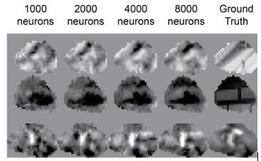
      As the reviewer points out, the diminishing returns of additional neurons to reconstruction performance is at least partly because there is redundancy in how a population of neurons represents visual stimuli. In supplementary figure S2, we inferred the on-off receptive fields of the neurons and show that visual space is oversampled in terms of the receptive field positions in panel C. However, the exact slope/shape of the performance vs population size curve we show in Figure 5 will also depend on the maximum performance of our reconstruction method, which is limited in spatial resolution (Figure 4 & Supplementary Figure S5). It is possible that future reconstruction approaches will require fewer neurons than ours, so we interpret this curve rather as a description of the reconstruction method itself than a feature of the underlying neuronal code. For that reason, we chose caution and refrained from making any claims about neuronal coding principles based on this plot. 

      (4) We appreciated the experiments testing the capacity of the reconstruction process, by using synthetic stimuli created under a Gaussian process in a noise-free way. But this originally further raised questions: what is the theoretical capability for reconstruction of this processing pipeline, as a whole? Is 0.563 the best that one could achieve given the noisiness and/or neuron count of the Sensorium project? What if the team applied the pipeline to reconstruct the activity of a given artificial neural network's layer (e.g., some ResNet convolutional layer), using hidden units as proxies for neuronal calcium activity? In the revision, this concern was addressed nicely in the review in Supplementary Figure 3C. Also, one appreciates that as a follow up, the team produced error maps (New Figure 6) that highlight where in the frames the reconstruction are likely to fail. But the maps went unanalyzed further, and I am not sure if there was a systematic trend in the errors. 

      We are happy to hear that we were able to answer the reviewers’ question of what the maximum theoretical performance of our reconstruction process is in figure 3C. Regarding systematic trends in the error maps, we also did not observe any clear systematic trends. If anything, we noticed that some moving edges were shifted, but we do not think we can quantify this effect with this particular dataset. 

      (5) I was encouraged by Figure 4, which shows how the reconstructions succeeded or failed across different spatial frequencies. The authors note that "the reconstruction process failed at high spatial frequencies," yet it also appears to struggle with low spatial frequencies, as the reconstructed images did not produce smooth surfaces (e.g., see the top rows of Figures 4A and 4B). In regions where one would expect a single continuous gradient, the reconstructions instead display specular, high-frequency noise. This issue is difficult to overlook and might deserve further discussion. 

      Thank you for pointing this out, this is indeed true. The reconstructions do have high frequency noise. We mention this briefly in line 102 “Finally, we applied a 3D Gaussian filter with sigma 0.5 pixels to remove the remaining static noise (Figure S3) and applied the evaluation mask.” In revisiting this sentence, we think it is more appropriate to replace “remove” with “reduce”. This noise is more visible in the Gaussian noise stimuli (Figure 4) because we did not apply the 3D Gaussian filter to these reconstructions, in case it interfered with the estimates of the reconstruction resolution limits. 

      Given that the Gaussian noise and drifting grating stimuli reconstructions were from predicted activity (“noise-free”), this high-frequency noise is not biological in origin and must therefore come from errors in our reconstruction process. This kind of high-frequency noise has previously been observed in feature visualization (optimizing input to maximize the activity of a specific node within a neural network to visualize what that node encodes; Olah, et al., "Feature Visualization", https://distill.pub/2017/feature-visualization/, 2017). It is caused by a kind of overfitting, whereby a solution to the optimization is found that is not “realistic”. Ways of combating this kind of noise include gradient smoothing, image smoothing, and image transformations during optimization, but these methods can restrict the resolution of the features that are recovered. Since we were more interested in determining the maximum resolution of stimuli that can be reconstructed in Figure 4 and Supplementary Figures 5-6, we chose not to apply these methods.

      Reviewer #3 (Public review): 

      Summary: 

      This paper presents a method for reconstructing input videos shown to a mouse from the simultaneously recorded visual cortex activity (two-photon calcium imaging data). The publicly available experimental dataset is taken from a recent brain-encoding challenge, and the (publicly available) neural network model that serves to reconstruct the videos is the winning model from that challenge (by distinct authors). The present study applies gradient-based input optimization by backpropagating the brain-encoding error through this selected model (a method that has been proposed in the past, with other datasets). The main contribution of the paper is, therefore, the choice of applying this existing method to this specific dataset with this specific neural network model. The quantitative results appear to go beyond previous attempts at video input reconstruction (although measured with distinct datasets). The conclusions have potential practical interest for the field of brain decoding, and theoretical interest for possible future uses in functional brain exploration. 

      Strengths: 

      The authors use a validated optimization method on a recent large-scale dataset, with a state-of-the-art brain encoding model. The use of an ensemble of 7 distinct model instances (trained on distinct subsets of the dataset, with distinct random initializations) significantly improves the reconstructions. The exploration of the relation between reconstruction quality and number of recorded neurons will be useful to those planning future experiments. 

      Weaknesses: 

      The main contribution is methodological, and the methodology combines pre-existing components without any new original component. 

      We thank the reviewer for their balanced assessment of our manuscript.


      The following is the authors’ response to the original reviews.

      Public Reviews:

      Reviewer #1 (Public review): 

      Summary: 

      This paper presents a method for reconstructing videos from mouse visual cortex neuronal activity using a state-of-the-art dynamic neural encoding model. The authors achieve high-quality reconstructions of 10-second movies at 30 Hz from two-photon calcium imaging data, reporting a 2-fold increase in pixel-by-pixel correlation compared to previous methods. They identify key factors for successful reconstruction including the number of recorded neurons and model ensembling techniques. 

      Strengths: 

      (1) A comprehensive technical approach combining state-of-the-art neural encoding models with gradient-based optimization for video reconstruction. 

      (2) Thorough evaluation of reconstruction quality across different spatial and temporal frequencies using both natural videos and synthetic stimuli. 

      (3) Detailed analysis of factors affecting reconstruction quality, including population size and model ensembling effects. 

      (4) Clear methodology presentation with well-documented algorithms and reproducible code. 

      (5) Potential applications for investigating visual processing phenomena like predictive coding and perceptual learning. 

      We thank the reviewer for taking the time to provide this valuable feedback. We would like to add that in our eyes one additional main contribution is the step of going from reconstruction of static images to dynamic videos. We trust that in the revised manuscript, we have now made the point more explicit that static image reconstruction relies on temporally averaged responses, which negates the necessity of having to account for temporal dynamics altogether. 

      Weaknesses: 

      The main metric of success (pixel correlation) may not be the most meaningful measure of reconstruction quality: 

      High correlation may not capture perceptually relevant features.

      Different stimuli producing similar neural responses could have low pixel correlations The paper doesn't fully justify why high pixel correlation is a valuable goal 

      This is a very relevant point. In retrospect, perhaps we did not justify this enough. Sensory reconstruction typically aims to reconstruct sensory input based on brain activity as faithfully as possible. A brain-to-image decoder might therefore be trained to produce images as close to the original input as possible. The loss function to train the decoder would therefore be image similarity on the pixel level. In that case, evaluating reconstruction performance based on pixel correlation is somewhat circular. 

      However, when reconstructing videos, we optimize the input video in terms of its perceptual similarity to the original video and only then evaluate pixel-level similarity. The perceptual similarity metric we optimize for is the estimate of how the neurons in mouse V1 respond to that video. We then evaluate the similarity of this perceptually optimized video to the original input video with pixel-level correlation. In other words, we optimize for perceptual similarity and then evaluate pixel similarity. If our method optimized pixel-level similarity, then we would agree that perceptual similarity is a more relevant evaluation metric. We do not think it was clear in our original submission that our optimization loss function is a perceptual loss function, and have now made this clearer in Figure 1C-D and have clarified this in the results section, line 70:

      “In effect, we optimized the input video to be perceptually similar with respect to the recorded neurons.”

      And in line 110: 

      “Because our optimization of the movies was based on a perceptual loss function, we were interested in how closely these movies matched the originals on the pixel level.”

      We chose to use pixel correlation to measure pixel-level similarity for several reasons. 1) It has been used in the past to evaluate reconstruction performance (Yoshida et al., 2020), 2) It is contrast and luminance insensitive, 3) correlation is a common metric so most readers will have an intuitive understanding of how it relates to the data. 

      To further highlight why pixel similarity might be interesting to visualize, we have included additional analysis in Figure 6 illustrating pixel-level differences between reconstructions from experimentally recorded activity and predicted activity. 

      We expect that the type of perceptual similarity the reviewer is alluding to is pretrained neural network image embedding similarity (Zhang et al., 2018: https://doi.org/10.48550/arXiv.1801.03924). While these metrics seem to match human perceptual similarity, it is unclear if they reflect mouse vision. We did try to compare the embedding similarity from pretrained networks such as VGG16, but got results suggesting the reconstructed frames were no more similar to the ground truth than random frames, which is obviously not true. This might be because the ground truth videos were too different in resolution from the training data of these networks and because these metrics are typically very sensitive to decreases in resolution. 

      The best alternative approach to evaluate mouse perceptual similarity would be to show the reconstructed videos to the same animals while recording the same neurons and to compare these neural activation patterns to those evoked by the original ground truth videos. This has been done for static images in the past: Cobos et al., bioRxiv 2022, found that static image reconstructions generated using gradient descent evoked more similar trial-averaged (40 trials) responses to those evoked by ground truth images compared to other reconstruction methods. Unfortunately, we are currently not able to perform these in vivo experiments, which is why we used publicly available data for the current paper. We plan to use this method in the future. But this method is also not flawless as it assumes that the average response to an image is the best reflection of how that image is represented, which may not be the case for an individual trial.

      As far as we are aware, there is currently no method that, given a particular activity pattern in response to an image/video, can produce an image/video that induces a neural activity pattern that is closer to the original neural response than simply showing the same image/video again. Hypothetically, such a stimulus exists because of various visual processing phenomena we mention in our discussion (e.g., predictive coding and selective attention), which suggest that the image that is represented by a population of neurons likely differs from the original sensory input. In other words, what the brain represents is an interpretation of reality not a pure reflection. Experimentally verifying this is difficult, as these variations might be present on a single trial level. The first step towards establishing a method that captures the visual representation of a population of neurons is sensory reconstruction, where the aim is to get as close as possible to the original sensory input. We think pixel-level correlation is a stringent and interpretable metric for this purpose, particularly when optimizing for perceptual similarity rather than image similarity directly.

      Comparison to previous work (Yoshida et al.) has methodological concerns: Direct comparison of correlation values across different datasets may be misleading; Large differences in the number of recorded neurons (10x more in the current study); Different stimulus types (dynamic vs static) make comparison difficult; No implementation of previous methods on the current dataset or vice versa. 

      Yes, we absolutely agree that direct comparison to previous static image reconstruction methods is problematic. We primarily do so because we think it is standard practice to give related baselines. We agree that direct comparison of the performance of video reconstruction methods to image reconstruction methods is not really possible. It does not make sense to train and apply a dynamic model on a static image data set where neural activity is time-averaged, as the temporal kernels could not be learned. Conversely, for a static model, which expects a single image as input and predicts time averaged responses, it does not make sense to feed it a series of temporally correlated movie frames and to simply concatenate the resulting activity perdition. The static model would need to be substantially augmented to incorporate temporal dynamics, which in turn would make it a new method. This puts us in the awkward position of being expected to compare our video reconstruction performance to previous image reconstruction methods without a fair way of doing so. We have now added these caveats in line 119:

      “However, we would like to stress that directly comparing static image reconstruction methods with movie reconstruction approaches is fundamentally problematic, as they rely on different data types both during training and evaluation (temporally averaged vs continuous neural activity, images flashed at fixed intervals vs continuous movies).”

      We have also toned down the language, emphasising the comparison to previous image reconstruction performance in the abstract, results, and conclusion. 

      Abstract: We removed “We achieve a ~2-fold increase in pixel-by-pixel correlation compared to previous state-of-the-art reconstructions of static images from mouse V1, while also capturing temporal dynamics.” and replaced with “We achieve a pixel-level correction of 0.57 between the ground truth movie and the reconstructions from single-trial neural responses.”

      Discussion: we removed “In conclusion, we reconstruct videos presented to mice based on the activity of neurons in the mouse visual cortex, with a ~2-fold improvement in pixel-by-pixel correlation compared to previous static image reconstruction methods.” and replaced with “In conclusion, we reconstruct videos presented to mice based on single-trial activity of neurons in the mouse visual cortex.”

      We have also removed the performance table and have instead added supplementary figure 3 with in-depth comparison across different versions of our reconstruction method (variations of masking, ensembling, contrast & luminance matching, and Gaussian blurring). 

      Limited exploration of how the reconstruction method could provide insights into neural coding principles beyond demonstrating technical capability. 

      The aim of this paper was not to reveal principles of neural coding. Instead, we aimed to achieve the best possible performance of video reconstructions and to quantify the limitations. But to highlight its potential we have added two examples of how sensory reconstruction has been applied in human vision research in line 321: 

      “Although fMRI-based reconstruction techniques are starting to be used to investigate visual phenomena in humans (such as illusions [Cheng et al., 2023] and mental imagery [Shen et al., 2019; Koide-Majima et al., 2024; Kalantari et al., 2025]), visual processing phenomena are likely difficult to investigate using existing fMRI-based reconstruction approaches, due to the low spatial and temporal resolution of the data.”

      We have also added a demonstration of how this method could be used to investigate which parts of a reconstruction from a single trial response differs from the model's prediction (Figure  6). We do this by calculating pixel-level differences between reconstructions from the recorded neural activity and reconstructions from the expected neural activity (predicted activity by the neural encoding model). Although difficult to interpret, this pixel-by-pixel error map could represent trial-by-trial deviations of the neural code from pure sensory representation. But at this point we cannot know whether these errors are nothing more than errors in the reconstruction process. To derive meaningful interpretations of these maps would require a substantial amount of additional work and in vivo experiments and so is outside the scope of this paper, but we include this additional analysis now to highlight a) why pixel-level similarity might be interesting to quantify and visualize and b) to demonstrate how video reconstruction could be used to provide insights into neural coding, namely as a tool to identify how sensory representations differ from a pure reflection of the visual input.  

      The claim that "stimulus reconstruction promises a more generalizable approach" (line 180) is not well supported with concrete examples or evidence. 

      What we mean by generalizable is the ability to apply reconstruction to novel stimuli, which is not possible for stimulus classification. We now explain this better in the paragraph in line 211: 

      “Stimulus identification, i.e. identifying the most likely stimulus from a constrained set, has been a popular approach for quantifying whether a population of neurons encodes the identity of a particular stimulus [Földiák, 1993, Kay et al., 2008]. This approach has, for instance, been used to decode frame identity within a movie [Deitch et al., 2021, Xia et al., 2021, Schneider et al., 2023, Chen et al.,2024]. Some of these approaches have also been used to reorder the frames of the ground truth movie [Schneider et al., 2023] based on the decoded frame identity. Importantly, stimulus identification methods are distinct from stimulus reconstruction where the aim is to recreate what the sensory content of a neuronal code is in a way that generalizes to new sensory stimuli [Rakhimberdina et al., 2021]. This is inherently a more demanding task because the range of possible solutions is much larger. Although stimulus identification is a valuable tool for understanding the information content of a population code, stimulus reconstruction could provide a more generalizable approach, because it can be applied to novel stimuli.”

      All the stimuli we reconstructed were not in the training set of the model, i.e., novel. We have also downed down the claim: we have replaced “promises” with “could provide”. 

      The paper would benefit from addressing how the method handles cases where different stimuli produce similar neural responses, particularly for high-speed moving stimuli where phase differences might be lost in calcium imaging temporal resolution. 

      Thank you for this suggestion, we think this is a great question. Calcium dynamics are slow and some of the high temporal frequency information could indeed be lost, particularly phase information. In other words, when the stimulus has high temporal frequency information, it is harder to decode spatial information because of the slow calcium dynamics. Ideally, we would look at this effect using the drifting grating stimuli; however, this is problematic because we rely on predicted activity from the SOTA DNEM, and due to the dilation of the first convolution, the periodic grating stimulus causes aliasing. At 15Hz, when the temporal frequency of the stimulus is half the movie frame rate, the model is actually being given two static images, and so the predicted activity is the interleaved activity evoked by two static images. We therefore do not think using the grating stimuli is a good idea. But we have used the Gaussian stimuli as it is not periodic, and is therefore less of a problem. 

      We have now also reconstructed phase-inverted Gaussian noise stimuli and plotted the video correlation between the reconstructions from activity evoked by phase-inverted stimuli. On the one hand, we find that even for the fastest changing stimuli, the correlation between the reconstructions from phase inverted stimuli are negative, meaning phase information is not lost at high temporal frequencies. On the other hand, for the highest spatial frequency stimuli, the correlation is negative. So, the predicted neural activity (and therefore the reconstructions) are phase-insensitive when the spatial frequency is higher than the reconstruction resolution limit we identified (spatial length constant of 1 pixel, or 3.38 degrees). Beyond this limit, the DNEM predicts activity in response to phase-inverted stimuli, which, when used for reconstruction, results in movies which are more similar to each other than the stimulus that actually evokes them. 

      However, not all information is lost at these high spatial frequencies. If we plot the Shannon entropy in the spatial domain or the motion energy in the temporal domain, we find that even when the reconstructions fail to capture the stimulus at a pixel-specific level (spatial length constant of 1 pixel, or 3.38 degrees), they do capture the general spatial and temporal qualities of the videos. 

      We have added these additional analyses to Figure 4 and Supplementary Figure 5.

      Reviewer #2 (Public review): 

      This is an interesting study exploring methods for reconstructing visual stimuli from neural activity in the mouse visual cortex. Specifically, it uses a competition dataset (published in the Dynamic Sensorium benchmark study) and a recent winning model architecture (DNEM, dynamic neural encoding model) to recover visual information stored in ensembles of the mouse visual cortex. 

      This is a great project - the physiological data were measured at a single-cell resolution, the movies were reasonably naturalistic and representative of the real world, the study did not ignore important correlates such as eye position and pupil diameter, and of course, the reconstruction quality exceeded anything achieved by previous studies. Overall, it is great that teams are working towards exploring image reconstruction. Arguably, reconstruction may serve as an endgame method for examining the information content within neuronal ensembles - an alternative to training interminable numbers of supervised classifiers, as has been done in other studies. Put differently, if a reconstruction recovers a lot of visual features (maybe most of them), then it tells us a lot about what the visual brain is trying to do: to keep as much information as possible about the natural world in which its internal motor circuits may act consequently. 

      While we enjoyed reading the manuscript, we admit that the overall advance was in the range of those that one finds in a great machine learning conference proceedings paper. More specifically, we found no major technical flaws in the study, only a few potential major confounds (which should be addressable with new analyses), and the manuscript did not make claims that were not supported by its findings, yet the specific conceptual advance and significance seemed modest. Below, we will go through some of the claims, and ask about their potential significance. 

      We thank the reviewer for the positive feedback on our paper.

      (1) The study showed that it could achieve high-quality video reconstructions from mouse visual cortex activity using a neural encoding model (DNEM), recovering 10-second video sequences and approaching a two-fold improvement in pixel-by-pixel correlation over attempts. As a reader, I am left with the question: okay, does this mean that we should all switch to DNEM for our investigations of the mouse visual cortex? What makes this encoding model special? It is introduced as "a winning model of the Sensorium 2023 competition which achieved a score of 0.301... single-trial correlation between predicted and ground truth neuronal activity," but as someone who does not follow this competition (most eLife readers are not likely to do so, either), I do not know how to gauge my response. Is this impressive? What is the best achievable score, in theory, given data noise? Is the model inspired by the mouse brain in terms of mechanisms or architecture, or was it optimized to win the competition by overfitting it to the nuances of the data set? Of course, I know that as a reader, I am invited to read the references, but the study would stand better on its own if clarified how its findings depended on this model. 

      This is a very good point. We do not think that everyone should switch to using this particular DNEM to investigate the mouse visual cortex, but we think DNEMs and stimulus reconstruction in general has a lot of potential. We think static neural encoding models have already been demonstrated to be an extremely valuable tool to investigate visual coding (Walker et al., 2019; Yoshida et al., 2021; Willeke et al., bioRxiv 2023). DNEMs are less common, largely because they are very large and are technically more demanding to train and use. That makes static encoding models more practical for some applications, but they do not have temporal kernels and are therefore only used for static stimuli. They cannot, for instance, encode direction tuning, only orientation tuning. But both static and dynamic encoding models have advantages over stimulus classification methods which we outline in our discussion. Here we provide the first demonstration that previous achievements in static image reconstruction are transferable to movies.

      It has been shown in the past for static neural encoding models that choosing a better-performing model produces reconstructed static images that are closer to the original image (Pierzchlewicz et al., 2023). The factors in choosing this particular DNEM were its capacity to predict neural activity (benchmarked against other models), it was open source, and the data it was designed for was also available. 

      To give more context to the model used in the paper, we have included the following, line 348:

      “This model achieved an average single-trial correlation between predicted and ground truth neural activity of 0.291 during the competition, this was later improved to 0.301. The competition benchmark models achieved 0.106, 0.164 and 0.197 single-trial correlation, while the third and second place models achieved 0.243 and 0.265. Across the models, a variety of architectural components were used, including 2D and 3D convolutional layers, recurrent layers, and transformers, to name just a few.” 

      Concerning biologically inspired model design. The winning model contained 3 fully connected layers comprising the “Cortex” just before the final readout of neural activity, but we would consider this level of biological inspiration as minor. We do not think that the exact architecture of the model is particularly important, as the crucial aspect of such neural encoders is their ability to predict neural activity irrespective of how they achieve it. There has been a move towards creating foundation models of the brain (Wang et al., 2025) and the priority so far has been on predictive performance over mechanistic interpretability or similarity to biological structures and processes. 

      Finally, we would like to note that we do not know what the maximum theoretical score for single-trial responses might be, and don't think there is a good way of estimating it in this context. 

      (2) Along those lines, two major conclusions were that "critical for high-quality reconstructions are the number of neurons in the dataset and the use of model ensembling." If true, then these principles should be applicable to networks with different architectures. How well can they do with other network types? 

      This is a good question. Our method critically relies on the accurate prediction of neural activity in response to new videos. It is therefore expected that a model that better predicts neural responses to stimuli will also be better at reconstructing those stimuli given population activity. This was previously shown for static images (Pierzchlewicz et al., 2023). It is also expected that whenever the neural activity is accurately predicted, the corresponding reconstructed frames will also be more similar to the ground truth frames. We have now demonstrated this relationship between prediction accuracy and reconstruction accuracy in supplementary figure 4.

      Although it would be interesting to compare the movie reconstruction performance of many different models with different architectures and activity prediction performances, this would involve quite substantial additional work because movie reconstruction is very resource- and time-intensive. Finding optimal hyperparameters to make such a comparison fair and informative would therefore be impractical and likely not yield surprising results. 

      We also think it is unlikely that ensembling would not improve reconstruction performance in other models because ensembling across model predictions is a common way of improving single-model performance in machine learning. Likewise, we think it is unlikely that the relationship between neural population size and reconstruction performance would differ substantially when using different models, because using more neurons means that a larger population of noisy neurons is “voting” on what the stimulus is. However, we would expect that if the model were worse at predicting neural activity, then more neurons are needed for an equivalent reconstruction performance. In general, we would recommend choosing the best possible DNEM available, in terms of neural activity prediction performance, when reconstructing movies using input optimization through gradient descent. 

      (3) One major claim was that the quality of the reconstructions depended on the number of neurons in the dataset. There were approximately 8000 neurons recorded per mouse. The correlation difference between the reconstruction achieved by 1 neuron and 8000 neurons was ~0.2. Is that a lot or a little? One might hypothesize that ~7,999 additional neurons could contribute more information, but perhaps, those neurons were redundant if their receptive fields were too close together or if they had the same orientation or spatiotemporal tuning. How correlated were these neurons in response to a given movie? Why did so many neurons offer such a limited increase in correlation? 

      In the population ablation experiments, we compared the performance using ~1000, ~2000, ~4000, ~8000 neurons, and found an attenuation of 39.5% in video correlation when dropping 87.5% of the neurons (~1000 neurons remaining), we did not try reconstruction using just 1 neuron. 

      (4) On a related note, the authors address the confound of RF location and extent. The study resorted to the use of a mask on the image during reconstruction, applied during training and evaluation (Line 87). The mask depends on pixels that contribute to the accurate prediction of neuronal activity. The problem for me is that it reads as if the RF/mask estimate was obtained during the very same process of reconstruction optimization, which could be considered a form of double-dipping (see the "Dead salmon" article, https://doi.org/10.1016/S1053-8119(09)71202-9). This could inflate the reconstruction estimate. My concern would be ameliorated if the mask was obtained using a held-out set of movies or image presentations; further, the mask should shift with eye position, if it indeed corresponded to the "collective receptive field of the neural population." Ideally, the team would also provide the characteristics of these putative RFs, such as their weight and spatial distribution, and whether they matched the biological receptive fields of the neurons (if measured independently). 

      We can reassure the reviewer that there is no double-dipping. We would like to clarify that the mask was trained only on videos from the training set of the DNEM and not the videos which were reconstructed. We have added the sentence, line 91: 

      “None of the reconstructed movies were used in the optimization of this transparency mask.”

      Making the mask dependent on eye position would be difficult to implement with the current DNEM, where eye position is fed to the model as an additional channel. When using a model where the image is first transformed into retinotopic coordinates in an eye position-dependent manner (such as in Wang et al., 2025) the mask could be applied in retinotopic coordinates and therefore be dependent on eye position. 

      Effectively, the alpha mask defines the relative level of influence each pixel contributes to neural activity prediction. We agree it is useful to compare the shape of the alpha mask with the location of traditional on-off receptive fields (RFs) to clarify what the alpha mask represents and characterise the neural population available for our reconstructions. We therefore presented the DNEM with on-off patches to map the receptive fields of single neurons in an in silico experiment (the experimentally derived RF are not available). As expected, there is a rough overlap between the alpha mask (Supplementary Figure 2D), the average population receptive field (Supplementary Figure 2B), and the location of receptive field peaks (Supplementary Figure 2C). In principle, all three could be used during training or evaluation for masking, but we think that defining a mask based on the general influence of images on neural activity, rather than just on off patch responses, is a more elegant solution.

      One idea of how to go a step further would be to first set the alpha mask threshold during training based on the % loss of neural activity prediction performance that threshold induces (in our case alpha=0.5 corresponds to ~3% loss in correlation between predicted vs recorded neural responses, see Supplementary Figure 3D), and second base the evaluation mask on a pixel correlation threshold (see example pixel correlation map in Supplementary Figure 2E) instead to avoid evaluating areas of the image with low image reconstruction confidence. 

      We referred to this figure in the result section, line 83:

      “The transparency masks are aligned with but not identical to the On-Off receptive field distribution maps using sparse-noise (Figure S2).” 

      We have also done additional analysis on the effect of masking during training and evaluation with different thresholds in Supplementary Figure 3.

      (5) We appreciated the experiments testing the capacity of the reconstruction process, by using synthetic stimuli created under a Gaussian process in a noise-free way. But this further raised questions: what is the theoretical capability for the reconstruction of this processing pipeline, as a whole? Is 0.563 the best that one could achieve given the noisiness and/or neuron count of the Sensorium project? What if the team applied the pipeline to reconstruct the activity of a given artificial neural network's layer (e.g., some ResNet convolutional layer), using hidden units as proxies for neuronal calcium activity? 

      That’s a very interesting point. It is very hard to know what the theoretical best reconstruction performance of the model would be. Reconstruction performance could be decreased due to neural variability, experimental noise, the temporal kernel of the calcium indicator and the imaging frame rate, information compression along the visual hierarchy, visual processing phenomena (such as predictive coding and selective attention), failure of the model to predict neural activity correctly, or failure of the reconstruction process to find the best possible image which explains the neural activity. We don't think we can disentangle the contribution of all these sources, but we can provide a theoretical maximum assuming that the model and the reconstruction process are optimal. To that end, we performed additional simulations and reconstructed the natural videos using the predicted activity of the neurons in response to the natural videos as the target (similar to the synthetic stimuli) and got a correlation of 0.766. So, the single trial performance of 0.569 is ~75% of this theoretical maximum. This difference can be interpreted as a combination of the losses due to neuronal variability, measurement noise, and actual deviations in the images represented by the brain compared to reality. 

      We thank the reviewer for this suggestion, as it gave us the idea of looking at error maps (Figure 6), where the pixel-level deviation of the reconstructions from recorded vs predicted activity is overlaid on the ground truth movie.

      (6) As the authors mentioned, this reconstruction method provided a more accurate way to investigate how neurons process visual information. However, this method consisted of two parts: one was the state-of-the-art (SOTA) dynamic neural encoding model (DNEM), which predicts neuronal activity from the input video, and the other part reconstructed the video to produce a response similar to the predicted neuronal activity. Therefore, the reconstructed video was related to neuronal activity through an intermediate model (i.e., SOTA DNEM). If one observes a failure in reconstructing certain visual features of the video (for example, high-spatial frequency details), the reader does not know whether this failure was due to a lack of information in the neural code itself or a failure of the neuronal model to capture this information from the neural code (assuming a perfect reconstruction process). Could the authors address this by outlining the limitations of the SOTA DNEM encoding model and disentangling failures in the reconstruction from failures in the encoding model? 

      To test if a better neural prediction by the DNEM would result in better reconstructions, we ran additional simulations and now show that neural activity prediction performance correlates with reconstruction performance (Supplementary Figure 4B). This is consistent with Pierzchlewicz et al., (2023) who showed that static image reconstructions using better encoding models leads to better reconstruction performance. As also mentioned in the answer to the previous comment, untangling the relative contributions of reconstruction losses is hard, but we think that improvements to the DNEM performance are key. Two suggestions to improving the DNEM we used would be to translate the input image into retinotopic coordinates and shift this image relative to eye position before passing it to the first convolutional layer (as is done in Wang et al. 2025), to use movies which are not spatially down sampled as heavily, to not use a dilation of 2 in the temporal convolution of the first layer and to train on a larger dataset. 

      (7) The authors mentioned that a key factor in achieving high-quality reconstructions was model assembling. However, this averaging acts as a form of smoothing, which reduces the reconstruction's acuity and may limit the high-frequency content of the videos (as mentioned in the manuscript). This averaging constrains the tool's capacity to assess how visual neurons process the low-frequency content of visual input. Perhaps the authors could elaborate on potential approaches to address this limitation, given the critical importance of high-frequency visual features for our visual perception. 

      This is exactly what we also thought. To answer this point more specifically, we ran additional simulations where we also reconstruct the movies using gradient ensembling instead of reconstruction ensembling. Here, the gradients of the loss with respect to each pixel of the movie is calculated for each of the model instances and are averaged at every iteration of the reconstruction optimization. In essence, this means that one reconstruction solution is found, and the averaging across reconstructions, which could degrade high-frequency content, is skipped. The reconstructions from both methods look very similar, and the video correlation is, if anything, slightly worse (Supplemental Figure 3A&C). This indicates that our original ensembling approach did not limit reconstruction performance, but that both approaches can be used, depending on what is more convenient given hardware restrictions. 

      Reviewer #3 (Public review): 

      Summary: 

      This paper presents a method for reconstructing input videos shown to a mouse from the simultaneously recorded visual cortex activity (two-photon calcium imaging data). The publicly available experimental dataset is taken from a recent brain-encoding challenge, and the (publicly available) neural network model that serves to reconstruct the videos is the winning model from that challenge (by distinct authors). The present study applies gradient-based input optimization by backpropagating the brain-encoding error through this selected model (a method that has been proposed in the past, with other datasets). The main contribution of the paper is, therefore, the choice of applying this existing method to this specific dataset with this specific neural network model. The quantitative results appear to go beyond previous attempts at video input reconstruction (although measured with distinct datasets). The conclusions have potential practical interest for the field of brain decoding, and theoretical interest for possible future uses in functional brain exploration. 

      Strengths: 

      The authors use a validated optimization method on a recent large-scale dataset, with a state-of-the-art brain encoding model. The use of an ensemble of 7 distinct model instances (trained on distinct subsets of the dataset, with distinct random initializations) significantly improves the reconstructions. The exploration of the relation between reconstruction quality and the number of recorded neurons will be useful to those planning future experiments. 

      Weaknesses: 

      The main contribution is methodological, and the methodology combines pre-existing components without any new original components. 

      We thank the reviewer for taking the time to review our paper and for their overall positive assessment. We would like to emphasise that combining pre-existing machine learning techniques to achieve top results in a new modality does require iteration and innovation. While gradient-based input optimization by backpropagating the brain-encoding error through a neural encoding model has been used in 2D static image optimization to generate maximally exciting images and reconstruct static images, we are the first to have applied it to movies which required accounting for the time domain. Previous methods used time averaged responses and were limited to the reconstruction of static images presented with fixed image intervals.

      The movie reconstructions include a learned "transparency mask" to concentrate on the most informative area of the frame; it is not clear how this choice impacts the comparison with prior experiments. Did they all employ this same strategy? If not, shouldn't the quantitative results also be reported without masking, for a fair comparison? 

      Yes, absolutely. All reconstruction approaches limit the field of view in some way, whether this is due to the size of the screen, the size of the image on the screen, or cropping of the presented/reconstructed images during analysis due to the retinotopic coverage of the recorded neurons. Note that we reconstruct a larger field of view than Yoshida et al. In Yoshida et al., the reconstructed field of view was 43 by 43 retinal degrees. we show the size of an example evaluation mask in comparison. 

      To address the reviewer’s concern more specifically, we performed additional simulations and now also show the performance using a variety of different training and evaluation masks, including different alpha thresholds for training and evaluation masks as well as the effective retinotopic coverage at different alpha thresholds. Despite these comparisons, we would also like to highlight that the comparison to the benchmark is problematic itself. This is because image and movie reconstruction are not directly comparable. It does not make sense to train and apply a dynamic model on a static image dataset where neural activity is time averaged. Conversely, it does not make sense to train or apply a static model that expects time-averaged neural responses on continuous neural activity unless it is substantially augmented to incorporate temporal dynamics, which in turn would make it a new method. This puts us in the awkward position of being expected to compare our video reconstruction performance to previous image reconstruction methods without a fair way of doing so. We have therefore de-emphasised the phrasing comparing our method to previous publications in the abstract, results, and discussion. 

      Abstract: “We achieve a ~2-fold increase in pixel-by-pixel correlation compared to previous state-of-the-art reconstructions of static images from mouse V1, while also capturing temporal dynamics.” with “We achieve a pixel-level correction of 0.57 between the ground truth movie and the reconstructions from single-trial neural responses.”

      Results: “This represents a ~2x higher pixel-level correlation over previous single-trial static image reconstructions from V1 in awake mice (image correlation 0.238 +/- 0.054 s.e.m for awake mice) [Yoshida et al., 2020] over a similar retinotopic area (~43° x 43°) while also capturing temporal dynamics. However, we would like to stress that directly comparing static image reconstruction methods with movie reconstruction approaches is fundamentally problematic, as they rely on different data types both during training and evaluation (temporally averaged vs continuous neural activity, images flashed at fixed intervals vs continuous movies).”

      Discussion: “In conclusion, we reconstruct videos presented to mice based on the activity of neurons in the mouse visual cortex, with a ~2-fold improvement in pixel-by-pixel correlation compared to previous static image reconstruction methods.” with “In conclusion, we reconstruct videos presented to mice based on single-trial activity of neurons in the mouse visual cortex.”

      We have also removed the performance table and have instead added supplementary figure 3 with in-depth comparison across different versions of our reconstruction method (variations of masking, ensembling, contrast & luminance matching, and Gaussian blurring). 

      We believe that we have given enough information in our paper now so that readers can make an informed decision whether our movie reconstruction method is appropriate for the questions they are interested in.

      Recommendations for the authors:

      Reviewer #2 (Recommendations for the authors): 

      (1) "Reconstructions have been luminance (mean pixel value across video) and contrast (standard deviation of pixel values across video) matched to ground truth." This was not clear: was it done by the investigating team? I imagine that one of the most easily captured visual features is luminance and contrast, why wouldn't the optimization titrate these well? 

      The contrast and luminance matching of the reconstructions to the ground truth videos was done by us, but this was only done to help readers assess the quality of the reconstructions by eye. Our performance metrics (frame and video correlation) are contrast and luminance insensitive. To clarify this, we have also added examples of non-adjusted frames in Supplementary Figure 3A, and added a sentence in the results, line 103: 

      “When presenting videos in this paper we normalize the mean and standard deviation of the reconstructions to the average and standard deviation of the corresponding ground truth movie before applying the evaluation masks, but this is not done for quantification except in Supplementary Figure 3D.”

      We were also initially surprised that contrast and luminance are not captured well by our reconstruction method, but this makes sense as V1 is largely luminance invariant (O’Shea et al., 2025 https://doi.org/10.1016/j.celrep.2024.115217 ) and contrast only has a gain effect on V1 activity (Tring et al., 2024 https://journals.physiology.org/doi/full/10.1152/jn.00336.2024). Decoding absolute contrast is likely unreliable because it is probably not the only factor modulating the overall gain of the neural population.

      To address the reviewer’s comment more fully, we ran additional experiments. More specifically, to test why contrast and luminance are not recovered in the reconstructions, we checked how the predicted activity between the reconstruction and the contrast/luminance corrected reconstructions differs. Contrast and luminance adjustment had little impact on predicted response similarity on average. This makes the reconstruction optimization loss function insensitive to overall contrast and luminance so it cannot be decoded. There is a small effect on activity correlation, however, so we cannot completely rule out that contrast and luminance could be reconstructed with a different loss function. 

      (2) The authors attempted to investigate the variability in reconstruction quality across different movies and 10-second snippets of a movie by correlating various visual features, such as video motion energy, contrast, luminance, and behavioral factors like running speed, pupil diameter, and eye movement, with reconstruction success. However, it would also be beneficial if the authors correlated the response loss (Poisson loss between neural responses) with reconstruction quality (video correlation) for individual videos, as these metrics are expected to be correlated if the reconstruction captures neural variance. 

      We thank the reviewer for this suggestion. We have now included this analysis and find that if the neural activity was better predicted by the DNEM then the reconstruction of the video was also more similar to the ground truth video. We further found that this effect is shift-dependent (in time), meaning the prediction of activity based on proximal video frames is more influential on reconstruction performance. 

      Reviewer #3 (Recommendations for the authors): 

      (1) I was confused about the choice of applying a transparency mask thresholded with alpha>0.5 during training and alpha>1 during evaluation. Why treat the two situations differently? Also, shouldn't we expect alpha to be in the [0,1] range, in which case, what is the meaning of alpha>1? (And finally, as already described in "Weaknesses", how does this choice impact the comparison with prior experiments? Did they also employ a similar masking strategy?) 

      We found that applying a mask during training increased performance regardless of the size of the evaluation mask. Using a less stringent mask during training than during evaluation increases performance slightly, but also allows inspection of the reconstruction in areas where the model will be less confident without sacrificing performance, if this is desired. The thresholds of 0.5 and 1 were chosen through trial and error, but the exact values do not hold intrinsic meaning. The alpha mask values can go above 1 during their optimization. We could have clipped alpha during the training procedure (algorithm 1), but we decided this was not worth redoing at this stage, as the alphas used for testing were not above 1. All reconstruction approaches in previous publications limit the field of view in some form, whether this is due to the size of the screen, the size of the image on the screen, or the cropping of the presented/reconstructed images during analysis. 

      To address the reviewer’s comment in detail, we have added extensive additional analysis to evaluate the coverage of the reconstruction achieved in this paper and how different masking strategies affect performance, as well as how the mask relates to more traditional receptive field mapping.  

      (2) I would not use the word "imagery" in the first sentence of the abstract, because this might be interpreted by some readers as reconstruction of mental imagery, a very distinct question. 

      We changed imagery to images in the abstract.

      (3) Line 145-146: "<1 frame, or <30Hz" should be "<1 frame, or >30Hz". 

      We have corrected the error.

      (4) Algorithm 1, Line 5, a subscript variable 'g' should be changed to 'h'

      We have corrected the error.

      Additional Changes

      (1) Minor grammatical errors

      (2) Addition of citations: We were previously not aware of a bioRxiv preprint from 2022 (Cobos et al., 2022), which used gradient descent-based input optimization to reconstruct static images but without the addition of a diffusion model. Instead, we had cited for this method Pierzchlewicz et al., 2023 bioRxiv/NeurIPS. In Cobos et al., 2022, they compare static image reconstruction similarity to ground truth images and the similarity of the in vivo evoked activity across multiple reconstruction methods. Performance values are only given for reconstructions from trial-averaged responses across ~40 trials (in the absence of original data or code we are also not able to retrospectively calculate single-trial performance). The authors find that optimizing for evoked activity rather than image similarity produces image reconstructions that evoke more similar in vivo responses compared to reconstructions optimized for image similarity itself. We have now added and discussed the citation in the main text. 

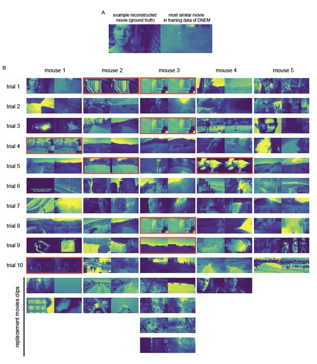
      (3) Workaround for error in the open-source code from https://github.com/lRomul/sensorium for video hashing function in the SOTA DNEM: By checking the most correlated first frame for each reconstructed movie, we discovered there was a bug in the open-source code and 9/50 movies we originally used for reconstruction were not properly excluded from the training data between DNEM instances. The reason for this error was that some of the movies are different by only a few pixels, and the video hashing function used to split training and test set folds in the original DNEM code classified these movies as different and split them across folds. We have replaced these 9 movies and provide a figure below showing the next closest first frame for every movie clip we reconstruct. This does not affect our claims. Excluding these 9 movie clips, did not affect the reconstruction performance (video correlation went from 0.563 to 0.568), so there was no overestimation of performance due to test set contamination. However, they should still be removed so some of the values in the paper have changed slightly. The only statistical test that was affected was the correlation between video correlation and mean motion energy (Supplementary Figure 4A), which went from p = 0.043 to 0.071. 

      Author response image 2.

      exclusion of movie clips with duplicates in the DNEM training data. A) example frame of a reconstructed movie (ground truth) and the most correlated first frame from the training data. b) all movie clips and their corresponding most correlated clip from the training data. Red boxes indicate excluded duplicates. 

    1. The LLM predicts continuations that match those high-quality human patterns.

      but spotting errors in proofs? how can just predicitng patterns do that?

    2. predicting sequences that humans label as correct solutions.

      Does that mean if there's a very new question, then the model would fail to solv? but the truth is LLMs like Gemini deepthink are still surpassing PhDs in solving them

    3. advanced models produce remarkably sophisticated outputs. How might that emerge purely from prediction?

      The language seems to be sophisticated to humans, because the models have been trained and post-trained and tuned towards outputs which seem readable and actually more pleasing to humans. But I'm still unsure how in math, or debugging, do they generate correct, useful outputs?

    4. —how might that guide your own use?

      BUt I am confused. I have used LLMs to extract insights/inaccuracies (in math), generate novel brainstorming questions, reviews,even generate prompts (prompt engineering). it doesnt seem they were just predicitng next word

    1. To unlock this flexibility, Germany must expand storage options and ensure users can respond to power availability. A key step came with the obligation for electricity suppliers to offer at least one dynamic tariff from 2025, but additional incentives must follow. As Germany paves the way towards covering 80 percent of its electricity demand with renewables by 2030, measures and proposals for 2026 to unlock flexibility include

      I Totally missed this. It’s an obligation now?

    1. Note: This response was posted by the corresponding author to Review Commons. The content has not been altered except for formatting.

      Learn more at Review Commons


      Reply to the reviewers

      1. General Statements

      We thank the reviewers for their overall support, thorough review, and thoughtful comments. The points raised were all warranted and we feel that addressing them has improved the quality of our manuscript. Below we respond to each of the points raised.

      2. Point-by-point description of the revisions

      Reviewer #1

      Minor comments:

      Are the lgl-1; pac-1 M-Z- double mutants dead? Only the phenotype of pac-1(M-Z-); lgl-1 (M+Z-) is shown. In figures and text throughout, it should be clear whether mutants are referring to zygotic loss or both maternal and zygotic loss, as this distinction could have major implications on the interpretation of experiments.

      Almost all experiments we performed used a combination of RNAi of lgl-1 in a homozygous pac-1 null mutant background, or the other way around. RNAi should eliminate maternal product, but we hesitate to use the terminology M/Z since it has previously been used for protein degradation strategies.

      We have updated the text and figure 1 to address the potential of maternal product masking earlier phenotypes, and performed additional RNAi experiments to demonstrate that the phenotypes obtained by RNAi for either pac-1 or lgl-1 in a homozygous mutant background for the other are the same as for the genetic double mutant. The results are shown as additional images and quantifications in figure 1B,C. We also updated the legend to figure 1 to make it clear that double genetic mutants are obtained from heterozygous lgl-1/+ parents.

      Regarding the phenotype of lgl-1; pac-1 M-Z- double mutants: assuming the reviewer refers to M-Z- double genetic mutants, we cannot make such embryos as the pac-1(M-Z-); lgl-1(M+Z-) animals are already lethal.

      In Figure 1C, it would be more appropriate to show a fully elongated WT embryo to contrast with arrested elongation in mutant embryos.

      We agree with the reviewer and have replaced the 2-fold WT embryo with a 3-fold embryo.

      Is the lateral spread of DLG-1 in double mutant embryos a result of failure to polarize DLG-1, or failure to maintain polarity? This should be straightforward to address in higher time resolution movies.

      We have analyzed additional embryos at early stages of development. In lgl-1; pac-1 embryos we never see the appearance of complete junctions: defects are apparent already at dorsal intercalation. We interpret these results as a failure to properly polarize DLG-1. We have added additional images to Figure S2 and added this sentence to the text: Imaging of embryos from early stages of development on showed that normal continuous junctional DLG-1 bands are never established in pac-1(RNAi); lgl-1(mib201) embryos (Fig. S2B).

      The lack of enhancement of hmp-1(fe4) by lgl-1(RNAi) is quite interesting, given that pac-1 does enhance hmp-1(fe4). To rule out the possibility that this result stems from incomplete lgl-1 RNAi, this experiment should be repeated using the lgl-1 null mutant.

      We have done this experiment by recreating the fe4 S823F mutation in the lgl-1(null) mutant background as well as in the wild-type CGC1 background using CRISPR/Cas9. The phenotype of both was similar, but differs from that of the original PE97 strain. In the original strain, there is ~50% embryonic lethality but worms that complete embryogenesis grow up to be fertile adults. In our new "fe4" strains, nearly all animals are severely malformed with little to no elongation taking place. We are able to maintain both strains (with and without lgl-1) homozygous but with difficulty as only ~5% of animals grow up and give progeny. Apparently, there are genetic differences between PE97 and our CGC1 background that cause phenotypic differences despite having the same amino acid change in HMP-1.

      Nevertheless, using our original embryonic viability criterium of 'hatching', loss of lgl-1 does not enhance the S823F mutation. We have included the following text in the manuscript:

      To rule out that the lack of enhancement by lgl-1(RNAi) is due to incomplete inactivation of lgl-1, we also re-created the hmp-1(fe4) mutation (S823F) by CRISPR in lgl-1(mib201) mutant animals and wild-type controls. The phenotype of the S823F mutant we created is more severe than that of the original PE97 hmp-1(fe4) strain, with only ~5% of animals becoming fertile adults (Fig. S2F). This likely represents the presence of compensatory changes that have accumulated over time in PE97. Nevertheless, consistent with our RNAi results, the presence of lgl-1(mib201) did not further exacerbate the phenotype of HMP-1(S823F) (Fig. S2E, F). Taken together, the lack of enhancement of hmp-1(S823F) mutants by inactivation of loss of lgl-1 This observation argues against a primary role for lgl-1 in regulating cell junctions.

      • Related to point 4, do pac-1 or lgl-1 null mutants enhance partial knockdown of junction protein DLG-1, or is this effect (of pac-1) specific to HMP-1/AJs?*

      We have attempted to address this point using feeding RNAi against dlg-1. However, we were not able to obtain partial depletion of DLG-1. On RNAi feeding plates, control, pac-1, and lgl-1 animals did not show significant embryonic lethality. We checked RNAi effectiveness with a DLG-1::mCherry strain and found RNAi by feeding to be very ineffective. Since we could not deplete DLG-1 to a level that results in partial embryonic lethality, we were not able to address this question properly.

      Does lgl-1 loss affect PAC-1 protein localization and vice versa?

      It does not. We have added the following text and a figure panel: Loss-of-function mutants that strongly enhance a phenotype are often interpreted as acting in parallel pathways. We therefore examined whether loss of lgl-1 or pac-1 alters the localization of endogenously GFP-tagged LGL-1 or PAC-1. In neither null background did we detect changes in the subcellular localization of the other protein, consistent with LGL-1 and PAC-1 functioning in parallel pathways (Fig. S1D).

      Reviewer #2

      Very little of the imaging data are analyzed quantitatively, and in many cases it is not clear how many embryos were analyzed. While the images that are presented show clear defects, readers cannot determine how reproducible, strong or significant the phenotypes are.

      We completely agree with the reviewer that interpretation of our data requires this information and apologize for the omission in the first manuscript version. The phenotypes are highly penetrant and consistent (timing of arrest, % lethality, junctional defects), and we have now added quantifications throughout the manuscript.

      In particular, the data below should be quantified and, where possible, analyzed statistically:

      • The frequency of the various junctional phenotypes shown in 2C

      We have now quantified the junctional phenotypes. The junctional defects are highly penetrant: >90% of lgl-1; pac-1 embryos have junctional defects (new Fig. 2B). We used airy-scan confocal imaging to analyze the distribution of the different phenotypes (unaffected, spread laterally, and ring-like pattern). The results are shown in Fig. 2G.

      • The expansion of DLG-1::mCherry in pac-1 lgl-1 embryos should be quantified (related to Figure 2B). For example, the percentage of membrane (marked by PH::GFP) occupied by DLG-1 could be quantified.

      We have performed this quantification, shown in Fig. 2D.

      - Similarly, the expansion of the aPKC domain should be quantified (Figure 3A).

      An objective quantification of aPKC signal is difficult due to the relatively weak expression of aPKC::GFP and the lack of a clear demarcating boundary. This is part of the reason we measured tortuosity as a more quantifyable indicator of apical domain expansion. We have now added a qualitative observation table as Figure 3B. In addition, we have expanded the quantification of cell geometry by measuring lateral and basal surfaces. Lateral surfaces were decreased. We added the following text:

      To better understand the reason for the change in geometry, we also measured the lengths of the lateral and basal surfaces (Fig. 3F). We found that the absolute lengths of the apical surfaces were not significantly different between pac-1(RNAi); lgl-1(mib201) and control animals. Instead, the lengths of the lateral domain were reduced (Fig. 3F). Hence, the more dome-shaped appearance of epidermal cells in pac-1; lgl-1 double mutant animals is due to a decrease in lateral domain size, which is consistent with the observed lateral spreading of aPKC.

      • How many embryos were analyzed for each marker shown in Figure 2A, and what proportion showed the described phenotypes? This could be given in the text or in a panel.

      We have added these numbers to panel 2B, and indicated the percentage in the text.

      • The frequency of the various junctional phenotypes shown in 4F.

      To address this, we have changed figure 4F to show three types of phenotype (strong, mild, no phenotype) and added how frequently we observed each to the panels. In rescue experiments, 18/24 embryos showed no junctional defects, while 6/24 showed a mild defect (compared to 100% severe in non-rescued embryos). To make room for this and other quantifications in Figure 4, we moved the demonstration that PAC-1 is depleted by RNAi to supplemental figure S4.

      Because the genetic perturbations used are global (either deletions or RNAi), it is not established whether PAC-1/LGL-1 act in epidermal epithelial cells per se (versus an earlier requirement that manifests in epidermal epithelial cells). While I agree that this is the most likely scenario, other mechanisms are possible.

      Our experiments indeed use global depletion/deletion of lgl-1 and pac-1. We cannot exclude therefore that other tissues do not contribute to the epithelial phenotypes. We assume that other tissues would be affected as well, and in fact have observed abnormal looking pharynx tissue (see our response to reviewer 3 below for examples). As the epidermis is one of the first tissue to develop it is likely the first in which phenotypes become apparent.

      In particular, the overall GFP::aPKC levels appear notably higher in pac-1 lgl-1 embryos in Figure 3A. aPKC levels should be quantified to determine if this is true of pac-1 lgl-1 embryos. If so, couldn't that explain (or at least contribute to) the observed phenotypes?

      Overall higher levels could indeed contribute to the phenotype. However, we have now quantified total aPKC levels in control and pac-1; lgl-1 embryos found no difference between them. We have added the following text to the manuscript: To determine if increased expression of aPKC might explain the broadened apical localization, we measured total intensity levels of aPKC::GFP. However, we detected no differences in fluorescence levels between control and pac-1(RNAi); lgl-1(mib201) animals (Fig. S3B, C).

      Minor

      Figure 4: For completeness, please include the embryonic viability of pac-1 lgl-1 +/- embryos treated with EV and cdc-42(RNAi), as was done for pac-1 lgl-1 pkc-3(ts) in Figure 4E. Presumably the increased proportion of viable embryos with the lgl-1 deletion allele is reflected in an overall increase in embryonic viability.

      The embryonic viability indeed increases, but not as much as one might think because 15% of embryos die from the cdc-42 RNAi itself. The most important rescue argument is that we can obtain adult pac-1; lgl-1 animals with cdc-42 RNAi.

      We have now included the overall rescue and the following text: Overall, cdc-42 RNAi caused a mild increase in embryonic viability (Fig. 4A). However, total embryonic viability may underestimate rescue of pac-1; lgl-1 embryonic lethality, because it also includes the ~15% lethality caused by cdc-42 inactivation itself, even among animals wild type for lgl-1.

      The orientation of the inset images in Figures 2C, 3A and 3D is confusing. An illustration showing how these images are oriented relative to each other would be helpful.

      We have added a figure showing how the junctions are oriented in the figures (Fig. 2E). We have also added supplemental videos S3 and S4 that should illustrate the phenotype more clearly as well.

      For completeness, it would be good to test whether lgl-1(delta) is also synthetically lethal with picc-1(RNAi) (Zilberman 2017).

      We like this idea and had already looked into this. Lgl-1 and picc-1 are not synthetic lethal (see graph in word file submitted). However, PICC-1 is not the only junctional localization signal for PAC-1, as demonstrated by the Nance lab. We find the data interesting but feel that it deserves a more thorough structure/function investigation of PAC-1 than we can provide here. Therefore we would prefer not to include this data.

      Reviewer #3

      We thank the reviewer for their support of our manuscript.

      A few small areas to improve this manuscript:

      p. 6 like 139: "remain" should be "remaining"

      We have fixed this typo.

      Could the authors mention what is the phenotype of the 10% of pac-1 animals that die?

      Yes. They die with pleotropic phenotypes not resembling those of our pac-1; lgl-1 double mutant embryos. We have added examples of these to Figure S1.

      Based on the Supplemental figures, it made me curious to ask: Did the authors notice changes in dorsal epidermal fusions? Cadherin normally disappears in the dorsal hyp7 cells at this time. Did the timing of the fusions change at all?

      We haven't analyzed this in detail but our time-lapse videos show that dorsal fusions still take place and do not seem to be particularly delayed (overall development is slightly delayed but the delay in fusion is consistent with overall delay).

      Again, curiosity driven by the Supplemental figures: did the authors notice defects in apical regions of internal organs, like the pharynx or intestine? The CDC-42 biosensor is asymmetrical in the developing intestine. See: DOI: 10.1242/bio.056911

      We did not pay much attention to the intestine as PAC-1 is barely detectable in this tissue. The pharynx is formed, which we can easily detect in arrested embryos as we use GFP or BFP expressed under the myo-2 promoter to mark the deletion of pac-1. While we did not look closely, we do observe defects in pharynx development.

    2. Note: This preprint has been reviewed by subject experts for Review Commons. Content has not been altered except for formatting.

      Learn more at Review Commons


      Referee #2

      Evidence, reproducibility and clarity

      Summary: This study focuses on the polarization of epidermal epithelial cells in C. elegans. Whereas the basolateral polarity protein is LGL-1 is required for epithelial polarity in flies, LGL-1 is dispensable for polarization and viability in C. elegans. Through a whole-genome RNAi screen, Jarosinska et al discover that the depletion of the RhoGAP PAC-1 is synthetically lethal with an lgl-1 deletion mutant. pac-1 lgl-1 double mutants have significant polarity defects in the epidermal epithelial, including mislocalization of junctional markers and expansion of the apical aPKC domain. As a result pac-1 lgl-1 double mutants fail to maintain surface epithelial and arrest development. Genetic interaction data suggest that increased CDC42 and aPKC activity in pac-1 lgl-1 contributes, as least in part, to the polarity defects and resulting embryonic lethality.

      Major comments:

      Very little of the imaging data are analyzed quantitatively, and in many cases it is not clear how many embryos were analyzed. While the images that are presented show clear defects, readers cannot determine how reproducible, strong or significant the phenotypes are. In particular, the data below should be quantified and, where possible, analyzed statistically:

      • The frequency of the various junctional phenotypes shown in 2C
      • The expansion of DLG-1::mCherry in pac-1 lgl-1 embryos should be quantified(related to Figure 2B). For example, the percentage of membrane (marked by PH::GFP) occupied by DLG-1 could be quantified.
      • Similarly, the expansion of the aPKC domain should be quantified (Figure 3A).
      • How many embryos were analyzed for each marker shown in Figure 2A, and what proportion showed the described phenotypes? This could be given in the text or in a panel.
      • The frequency of the various junctional phenotypes shown in 4F.

      Because the genetic perturbations used are global (either deletions or RNAi), it is not established whether PAC-1/LGL-1 act in epidermal epithelial cells per se (versus an earlier requirement that manifests in epidermal epithelial cells). While I agree that this is the most likely scenario, other mechanisms are possible. In particular, the overall GFP::aPKC levels appear notably higher in pac-1 lgl-1 embryos in Figure 3A. aPKC levels should be quantified to determine if this is true of pac-1 lgl-1 embryos. If so, couldn't that explain (or at least contribute to) the observed phenotypes?

      Minor

      Figure 4: For completeness, please include the embryonic viability of pac-1 lgl-1 +/- embryos treated with EV and cdc-42(RNAi), as was done for pac-1 lgl-1 pkc-3(ts) in Figure 4E. Presumably the increased proportion of viable embryos with the lgl-1 deletion allele is reflected in an overall increase in embryonic viability.

      The orientation of the inset images in Figures 2C, 3A and 3D is confusing. An illustration showing how these images are oriented relative to each other would be helpful.

      For completeness, it would be good to test whether lgl-1(delta) is also synthetically lethal with picc-1(RNAi) (Zilberman 2017).

      Significance

      LGL-1 is a conserved polarity protein that is essential for viability in Drosophila. In contrast, lgl-1 mutants are viable and have weak polarity phenotypes in C. elegans. A previous study showed that LGL-1 acts redundantly with the posterior polarity proteins PAR-2 during establishment of anterior/posterior polarity in the one-cell worm embryo. Here, Jarosinska et al show that LGL-1 acts redundantly with another protein, the RhoGAP protein PAC-1, in the polarization of the embryonic epidermal epithelial. The strength of this study is the identification of redundant roles for PAC-1 and LGL-1, the apparent strength of the polarity defects in the double mutant and the broader implication that LGL-1 may act in a range of redundant, cell/tissue specific pathways to regulate polarity. The primary weakness of this study is the lack of quantification. Additionally, the aPKC and CDC42 genetic interaction data hint at potential pathways, but fall short of establishing LGL-1's or PAC-1's mechanism of action.

      Advance: This works identifies a redundant genetic interaction between LGL-1 and PAC-1. While the data require additional quantification, the phenotypes presented appear clear and strong. Although the molecular mechanism by which LGL-1 and PAC-1 act is not well established in the current work, the core observation is significant and should provide a foundation for future studies dissecting the molecular mechanisms.

      Audience: This work will be of interest to a broad audience. LGL-1 is conserved and its role in cell polarization and epithelial polarity is very actively studied, including in mammalian systems.

      Field of expertise. C elegans embryonic development; cell polarity.

    3. Note: This preprint has been reviewed by subject experts for Review Commons. Content has not been altered except for formatting.

      Learn more at Review Commons


      Referee #1

      Evidence, reproducibility and clarity

      In this manuscript, Jarosinska and colleagues address the roles of two polarity regulators, pac-1 and lgl-1, in C. elegans epidermal polarity. Loss of function mutations in either of these gene individually does not block polarization, but through a genome-wide RNAi screen, the authors find that pac-1 and lgl-1 enhance each other to cause apical-basal polarity defects and arrest during epidermal morphogenesis. The remainder of the paper focuses on testing genetic interactions between both proteins and AJ proteins (HMP-1) as well as apical proteins (CDC-42, PKC-3). These experiments reveal some interesting differences in how lgl-1 and pac-1 interface with junctional proteins (pac-1 enhances hmp-1 but lgl-1 does not) and apical proteins (lgl-1 suppresses pkc-3 or cdc-42 partial loss but pac-1 does not).

      Minor comments:

      1. Are the lgl-1; pac-1 M-Z- double mutants dead? Only the phenotype of pac-1(M-Z-); lgl-1 (M+Z-) is shown. In figures and text throughout, it should be clear whether mutants are referring to zygotic loss or both maternal and zygotic loss, as this distinction could have major implications on the interpretation of experiments.
      2. In Figure 1C, it would be more appropriate to show a fully elongated WT embryo to contrast with arrested elongation in mutant embryos.
      3. Is the lateral spread of DLG-1 in double mutant embryos a result of failure to polarize DLG-1, or failure to maintain polarity? This should be straightforward to address in higher time resolution movies.
      4. The lack of enhancement of hmp-1(fe4) by lgl-1(RNAi) is quite interesting, given that pac-1 does enhance hmp-1(fe4). To rule out the possibility that this result stems from incomplete lgl-1 RNAi, this experiment should be repeated using the lgl-1 null mutant.
      5. Related to point 4, do pac-1 or lgl-1 null mutants enhance partial knockdown of junction protein DLG-1, or is this effect (of pac-1) specific to HMP-1/AJs?
      6. Does lgl-1 loss affect PAC-1 protein localization and vice versa?

      Significance

      Overall, the manuscript provides additional insights into apical-basal polarization in C. elegans and demonstrates that lgl-1 is likely working in a similar way as in Drosophila, despite the lack of a phenotype in single lgl-1 mutants. I found the experiments to be done rigorously and interpretations of the data appropriate. All of my suggestions on improving the manuscript are minor; suggested experiments should be viewed as optional ways to strengthen the conclusions/impact of the study.

    1. Reviewer #2 (Public review):

      Sourmpis et al. present a study in which the importance of including certain inductive biases in the fitting of recurrent networks is evaluated with respect to the generalization ability of the networks when exposed to untrained perturbations.

      The work proceeds in three stages:

      (i) a simple illustration of the problem is made. Two reference (ground-truth) networks with qualitatively different connectivity, but similar observable network dynamics, are constructed, and recurrent networks with varying aspects of design similarity to the reference networks are trained to reproduce the reference dynamics. The activity of these trained networks during untrained perturbations is then compared to the activity of the perturbed reference networks. It is shown that, of the design characteristics that were varied, the enforced sign (Dale's law) and locality (spatial extent) of efference were especially important.

      (ii) The intuition from the constructed example is then extended to networks that have been trained to reproduce certain aspects of multi-region neural activity recorded from mice during a detection task with a working-memory component. A similar pattern is demonstrated, in which enforcing the sign and locality of efference in the fitted networks has an influence on the ability of the trained networks to predict aspects of neural activity during unseen (untrained) perturbations.

      (iii) The authors then illustrate the relationship between the gradient of the motor readout of trained networks with respect to the net inputs to the network units, and the sensitivity of the motor readout to small perturbations of the input currents to the units, which (in vivo) could be controlled optogenetically. The paper is concluded with a proposed use for trained networks, in which the models could be analyzed to determine the most sensitive directions of the network and, during online monitoring, inform a targeted optogenetic perturbation to bias behavior.

      The authors do not overstate their claims, and in general, I find that I agree with their conclusions.

    2. Author response:

      The following is the authors’ response to the original reviews.

      Public Reviews:

      Reviewer #1 (Public review)

      Major:

      (1) In line 76, the authors make a very powerful statement: 'σRNN simulation achieves higher similarity with unseen recorded trials before perturbation, but lower than the bioRNN on perturbed trials.' I couldn't find a figure showing this. This might be buried somewhere and, in my opinion, deserves some spotlight - maybe a figure or even inclusion in the abstract.

      We agree with the reviewer that these results are important. The failure of σRNN on perturbed data could be inferred from the former Figures 1E, 2C-E, and 3D. Following the reviewers' comments, we have tried to make this the most prominent message of Figure 1, in particular with the addition of the new panel E. We also moved Table 1 from the  Supplementary to the main text to highlight this quantitatively. 

      (2) It's mentioned in the introduction (line 84) and elsewhere (e.g., line 259) that spiking has some advantage, but I don't see any figure supporting this claim. In fact, spiking seems not to matter (Figure 2C, E). Please clarify how spiking improves performance, and if it does not, acknowledge that. Relatedly, in line 246, the authors state that 'spiking is a better metric but not significant' when discussing simulations. Either remove this statement and assume spiking is not relevant, or increase the number of simulations.

      We could not find the exact quote from the reviewer, and we believe that he intended to quote “spiking is better on all metrics, but without significant margins”. Indeed, spiking did not improve the fit significantly on perturbed trials, this is particularly true in comparison with the benefits of Dale’s law and local inhibition. As suggested by the reviewer, we rephrased the sentence from this quote and more generally the corresponding paragraphs in the intro (lines 83-87) and in the results (lines 245-271). Our corrections in the results sections are also intended to address the minor point (4) raised by the same reviewer.

      (3) The authors prefer the metric of predicting hits over MSE, especially when looking at real data (Figure 3). I would bring the supplementary results into the main figures, as both metrics are very nicely complementary. Relatedly, why not add Pearson correlation or R2, and not just focus on MSE Loss?

      In Figure 3 for the in-vivo data, we do not have simultaneous electrophysiological recordings and optogenetic stimulation in this dataset.  The two are performed on different recording sessions. Therefore, we can only compare the effect of optogenetics on the behavior, and we cannot compute Pearson correlation or R2 of the perturbed network activity. To avoid ambiguity, we wrote “For the sessions of the in vivo dataset with optogenetic perturbation that we considered, only the behavior of an animal is recorded” on line 294. 

      (4) I really like the 'forward-looking' experiment in closed loop! But I felt that the relevance of micro perturbations is very unclear in the intro and results. This could be better motivated: why should an experimentalist care about this forward-looking experiment? Why exactly do we care about micro perturbation (e.g., in contrast to non-micro perturbation)? Relatedly, I would try to explain this in the intro without resorting to technical jargon like 'gradients'.

      As suggested, we updated the last paragraph of the introduction (lines 88 - 95) to give better motivation for why algorithmically targeted acute spatio-temporal perturbations can be important to dissect the function of neural circuits. We also added citations to recent studies with targeted in vivo optogenetic stimulation. As far as we know the existing previous work targeted network stimulation mostly using linear models, while we used non-linear RNNs and their gradients.

      Minor:

      (1) In the intro, the authors refer to 'the field' twice. Personally, I find this term odd. I would opt for something like 'in neuroscience'.

      We implemented the suggested change: l.27 and l.30

      (2) Line 45: When referring to previous work using data-constrained RNN models, Valente et al. is missing (though it is well cited later when discussing regularization through low-rank constraints)

      We added the citation: l.45

      (3) Line 11: Method should be methods (missing an 's').

      We fixed the typo.

      (4) In line 250, starting with 'So far', is a strange choice of presentation order. After interpreting the results for other biological ingredients, the authors introduce a new one. I would first introduce all ingredients and then interpret. It's telling that the authors jump back to 2B after discussing 2C.

      We restructured the last two paragraphs of section 2.1, and we hope that the presentation order is now more logical.

      (5) The black dots in Figure 3E are not explained, or at least I couldn't find an explanation.

      We added an explanation in the caption of Figure 3E.

      Reviewer #2 (Public review):

      (1) Some aspects of the methods are unclear. For comparisons between recurrent networks trained from randomly initialized weights, I would expect that many initializations were made for each model variant to be compared, and that the performance characteristics are constructed by aggregating over networks trained from multiple random initializations. I could not tell from the methods whether this was done or how many models were aggregated.

      The expectation of the reviewer is correct, we trained multiple models with different random seeds (affecting both the weight initialization and the noise of our model) for each variant and aggregated the results. We have now clarified this in Methods 4.6. lines 658-662.

      (2) It is possible that including perturbation trials in the training sets would improve model performance across conditions, including held-out (untrained) perturbations (for instance, to units that had not been perturbed during training). It could be noted that if perturbations are available, their use may alleviate some of the design decisions that are evaluated here.

      In general, we agree with the reviewer that including perturbation trials in the training set would likely improve model performance across conditions. One practical limitation explaining partially why we did not do it with our dataset is the small quantity of perturbed trials for each targeted cortical area: the number of trials with light perturbations is too scarce to robustly train and test our models.

      More profoundly, to test hard generalizations to perturbations (aka perturbation testing), it will always be necessary that the perturbations are not trivially represented in the training data. Including perturbation trials during training would compromise our main finding: some biological model constraints improve the generalization to perturbation. To test this claim, it was necessary to keep the perturbations out of the training data.

      We agree that including all available data of perturbed and non-perturbed recordings would be useful to build the best generalist predictive system. It could help, for instance, for closed-loop circuit control as we studied in Figure 5. Yet, there too, it will be important for the scientific validation process to always keep some causal perturbations of interest out of the training set. This is necessary to fairly measure the real generalization capability of any model. Importantly, this is why we think out-of-distribution “perturbation testing” is likely to have a recurring impact in the years to come, even beyond the case of optogenetic inactivation studied in detail in our paper.

      Recommendation for the authors:

      Reviewer #1 (Recommendation for the authors):

      The code is not very easy to follow. I know this is a lot to ask, but maybe make clear where the code is to train the different models, which I think is a great contribution of this work? I predict that many readers will want to use the code and so this will improve the impact of this work.

      We updated the code to make it easier to train a model from scratch.

      Reviewer #2 (Recommendation for the authors):

      The figures are really tough to read. Some of that small font should be sized up, and it's tough to tell in the posted paper what's happening in Figure 2B.

      We updated Figures 1 and 2 significantly, in part to increase their readability. We also implemented the "Superficialities" suggestions.

    1. Reviewer #2 (Public review):

      Summary:

      This manuscript by Liakopoulou et al. presents a comprehensive investigation into the role of ATAD2 in regulating chromatin dynamics during spermatogenesis. The authors elegantly demonstrate that ATAD2, via its control of histone chaperone HIRA turnover, ensures proper H3.3 localization, chromatin accessibility, and histone-to-protamine transition in post-meiotic male germ cells. Using a new well-characterized Atad2 KO mouse model, they show that ATAD2 deficiency disrupts HIRA dynamics, leading to aberrant H3.3 deposition, impaired transcriptional regulation, delayed protamine assembly, and defective sperm genome compaction. The study bridges ATAD2's conserved functions in embryonic stem cells and cancer to spermatogenesis, revealing a novel layer of epigenetic regulation critical for male fertility.

      Strengths:

      The MS first demonstration of ATAD2's essential role in spermatogenesis, linking its expression in haploid spermatids to histone chaperone regulation by connecting ATAD2-dependent chromatin dynamics to gene accessibility (ATAC-seq), H3.3-mediated transcription, and histone eviction. Interestingly and surprisingly, sperm chromatin defects in Atad2 KO mice impair only in vitro fertilization but not natural fertility, suggesting unknown compensatory mechanisms in vivo.

      Weaknesses:

      The MS is robust and there are not big weaknesses

      The authors have addressed all the queries successfully.

    2. Author response:

      The following is the authors’ response to the original reviews.

      Public Reviews:

      Reviewer #1 (Public review): 

      Summary: 

      The authors analyzed the expression of ATAD2 protein in post-meiotic stages and characterized the localization of various testis-specific proteins in the testis of the Atad2 knockout (KO). By cytological analysis as well as the ATAC sequencing, the study showed that increased levels of HIRA histone chaperone, accumulation of histone H3.3 on post-meiotic nuclei, defective chromatin accessibility and also delayed deposition of protamines. Sperm from the Atad2 KO mice reduces the success of in vitro fertilization. The work was performed well, and most of the results are convincing. However, this manuscript does not suggest a molecular mechanism for how ATAD2 promotes the formation of testis-specific chromatin. 

      We would like to take this opportunity to highlight that the present study builds on our previously published work, which examined the function of ATAD2 in both yeast S. pombe and mouse embryonic stem (ES) cells (Wang et al., 2021). In yeast, using genetic analysis we showed that inactivation of HIRA rescues defective cell growth caused by the absence of ATAD2. This rescue could also be achieved by reducing histone dosage, indicating that the toxicity depends on histone over-dosage, and that HIRA toxicity, in the absence of ATAD2, is linked to this imbalance.

      Furthermore, HIRA ChIP-seq performed in mouse ES cells revealed increased nucleosome-bound HIRA, particularly around transcription start sites (TSS) of active genes, along with the appearance of HIRA-bound nucleosomes within normally nucleosome-free regions (NFRs). These findings pointed to ATAD2 as a major factor responsible for unloading HIRA from nucleosomes. This unloading function may also apply to other histone chaperones, such as FACT (see Wang et al., 2021, Fig. 4C).

      In the present study, our investigations converge on the same ATAD2 function in the context of a physiologically integrated mammalian system—spermatogenesis. Indeed, in the absence of ATAD2, we observed H3.3 accumulation and enhanced H3.3-mediated gene expression. Consistent with this functional model of ATAD2— unloading chaperones from histone- and non-histone-bound chromatin—we also observed defects in histone-toprotamine replacement.

      Together, the results presented here and in Wang et al. (2021) reveal an underappreciated regulatory layer of histone chaperone activity. Previously, histone chaperones were primarily understood as factors that load histones. Our findings demonstrate that we must also consider a previously unrecognized regulatory mechanism that controls assembled histone-bound chaperones. This key point was clearly captured and emphasized by Reviewer #2 (see below).

      Strengths:

      The paper describes the role of ATAD2 AAA+ ATPase in the proper localization of sperm-specific chromatin proteins such as protamine, suggesting the importance of the DNA replication-independent histone exchanges with the HIRA-histone H3.3 axis. 

      Weaknesses: 

      (1) Some results lack quantification. 

      We will consider all the data and add appropriate quantifications where necessary.

      (2) The work was performed well, and most of the results are convincing. However, this manuscript does not suggest a molecular mechanism for how ATAD2 promotes the formation of testis-specific chromatin. 

      Please see our comments above.

      Reviewer #2 (Public review): 

      Summary:

      This manuscript by Liakopoulou et al. presents a comprehensive investigation into the role of ATAD2 in regulating chromatin dynamics during spermatogenesis. The authors elegantly demonstrate that ATAD2, via its control of histone chaperone HIRA turnover, ensures proper H3.3 localization, chromatin accessibility, and histone-toprotamine transition in post-meiotic male germ cells. Using a new well-characterized Atad2 KO mouse model, they show that ATAD2 deficiency disrupts HIRA dynamics, leading to aberrant H3.3 deposition, impaired transcriptional regulation, delayed protamine assembly, and defective sperm genome compaction. The study bridges ATAD2's conserved functions in embryonic stem cells and cancer to spermatogenesis, revealing a novel layer of epigenetic regulation critical for male fertility. 

      Strengths:

      The MS first demonstration of ATAD2's essential role in spermatogenesis, linking its expression in haploid spermatids to histone chaperone regulation by connecting ATAD2-dependent chromatin dynamics to gene accessibility (ATAC-seq), H3.3-mediated transcription, and histone eviction. Interestingly and surprisingly, sperm chromatin defects in Atad2 KO mice impair only in vitro fertilization but not natural fertility, suggesting unknown compensatory mechanisms in vivo. 

      Weaknesses:

      The MS is robust and there are not big weaknesses 

      Reviewer #3 (Public review): 

      Summary: 

      The authors generated knockout mice for Atad2, a conserved bromodomain-containing factor expressed during spermatogenesis. In Atad2 KO mice, HIRA, a chaperone for histone variant H3.3, was upregulated in round spermatids, accompanied by an apparent increase in H3.3 levels. Furthermore, the sequential incorporation and removal of TH2B and PRM1 during spermiogenesis were partially disrupted in the absence of ATAD2, possibly due to delayed histone removal. Despite these abnormalities, Atad2 KO male mice were able to produce offspring normally. 

      Strengths:

      The manuscript addresses the biological role of ATAD2 in spermatogenesis using a knockout mouse model, providing a valuable in vivo framework to study chromatin regulation during male germ cell development. The observed redistribution of H3.3 in round spermatids is clearly presented and suggests a previously unappreciated role of ATAD2 in histone variant dynamics. The authors also document defects in the sequential incorporation and removal of TH2B and PRM1 during spermiogenesis, providing phenotypic insight into chromatin transitions in late spermatogenic stages. Overall, the study presents a solid foundation for further mechanistic investigation into ATAD2 function. 

      Weaknesses:

      While the manuscript reports the gross phenotype of Atad2 KO mice, the findings remain largely superficial and do not convincingly demonstrate how ATAD2 deficiency affects chromatin dynamics. Moreover, the phenotype appears too mild to elucidate the functional significance of ATAD2 during spermatogenesis. 

      We respectfully disagree with the statement that our findings are largely superficial. Based on our investigations of this factor over the years, it has become evident that ATAD2 functions as an auxiliary factor that facilitates mechanisms controlling chromatin dynamics (see, for example, Morozumi et al., 2015). These mechanisms can still occur in the absence of ATAD2, but with reduced efficiency, which explains the mild phenotype we observed.

      This function, while not essential, is nonetheless an integral part of the cell’s molecular biology and should be studied and brought to the attention of the broader biological community, just as we study essential factors. Unfortunately, the field has tended to focus primarily on core functional actors, often overlooking auxiliary factors. As a result, our decade-long investigations into the subtle yet important roles of ATAD2 have repeatedly been met with skepticism regarding its functional significance, which has in turn influenced editorial decisions.

      We chose eLife as the venue for this work specifically to avoid such editorial barriers and to emphasize that facilitators of essential functions do exist. They deserve to be investigated, and the underlying molecular regulatory mechanisms must be understood.

      (1) Figures 4-5: The analyses of differential gene expression and chromatin organization should be more comprehensive. First, Venn diagrams comparing the sets of significantly differentially expressed genes between this study and previous work should be shown for each developmental stage. Second, given the established role of H3.3 in MSCI, the effect of Atad2 knockout on sex chromosome gene expression should be analyzed. Third, integrated analysis of RNA-seq and ATAC-seq data is needed to evaluate how ATAD2 loss affects gene expression. Finally, H3.3 ChIP-seq should be performed to directly assess changes in H3.3 distribution following Atad2 knockout.  

      (1) In the revised version, we will include Venn diagrams to illustrate the overlap in significantly differentially expressed genes between this study and previous work. However, we believe that the GSEAs presented here provide stronger evidence, as they indicate the statistical significance of this overlap (p-values). In our case, we observed p-value < 0.01 (**) and p < 0.001 (***).

      (2) Sex chromosome gene expression was analyzed and is presented in Fig. 5C.

      (3) The effect of ATAD2 loss on gene expression is shown in Fig. 4A, B, and C as histograms, with statistical significance indicated in the middle panels.

      (4) Although mapping H3.3 incorporation across the genome in wild-type and Atad2 KO cells would have been informative, the available anti-H3.3 antibody did not work for ChIP-seq, at least in our hands. The authors of Fontaine et al., 2022, who studied H3.3 during spermatogenesis in mice, must have encountered the same problem, since they tagged the endogenous H3.3 gene to perform their ChIP experiments.

      (2) Figure 3: The altered distribution of H3.3 is compelling. This raises the possibility that histone marks associated with H3.3 may also be affected, although this has not been investigated. It would therefore be important to examine the distribution of histone modifications typically associated with H3.3. If any alterations are observed, ChIP-seq analyses should be performed to explore them further.

      Based on our understanding of ATAD2’s function—specifically its role in releasing chromatin-bound HIRA—in the absence of ATAD2 the residence time of both HIRA and H3.3 on chromatin increases. This results in the detection of H3.3 not only on sex chromosomes but across the genome. Our data provide clear evidence of this phenomenon. The reviewer is correct in suggesting that the accumulated H3.3 would carry H3.3-associated histone PTMs; however, we are unsure what additional insights could be gained by further demonstrating this point.

      (3) Figure 7: While the authors suggest that pre-PRM2 processing is impaired in Atad2 KO, no direct evidence is provided. It is essential to conduct acid-urea polyacrylamide gel electrophoresis (AU-PAGE) followed by western blotting, or a comparable experiment, to substantiate this claim. 

      Figure 7 does not suggest that pre-PRM2 processing is affected in Atad2 KO; rather, this figure—particularly Fig. 7B—specifically demonstrates that pre-PRM2 processing is impaired, as shown using an antibody that recognizes the processed portion of pre-PRM2. ELISA was used to provide a more quantitative assessment; however, in the revised manuscript we will also include a western blot image.

      (4) HIRA and ATAD2: Does the upregulation of HIRA fully account for the phenotypes observed in Atad2 KO? If so, would overexpression of HIRA alone be sufficient to phenocopy the Atad2 KO phenotype? Alternatively, would partial reduction of HIRA (e.g., through heterozygous deletion) in the Atad2 KO background be sufficient to rescue the phenotype? 

      These are interesting experiments that require the creation of appropriate mouse models, which are not currently available.

      (5) The mechanism by which ATAD2 regulates HIRA turnover on chromatin and the deposition of H3.3 remains unclear from the manuscript and warrants further investigation. 

      The Reviewer is absolutely correct. In addition to the points addressed in response to Reviewer #1’s general comments (see above), it would indeed have been very interesting to test the segregase activity of ATAD2 (likely driven by its AAA ATPase activity) through in vitro experiments using the Xenopus egg extract system described by Tagami et al., 2004. This system can be applied both in the presence and absence (via immunodepletion) of ATAD2 and would also allow the use of ATAD2 mutants, particularly those with inactive AAA ATPase or bromodomains. However, such experiments go well beyond the scope of this study, which focuses on the role of ATAD2 in chromatin dynamics during spermatogenesis.

      References:

      (1) Wang T, Perazza D, Boussouar F, Cattaneo M, Bougdour A, Chuffart F, Barral S, Vargas A, Liakopoulou A, Puthier D, Bargier L, Morozumi Y, Jamshidikia M, Garcia-Saez I, Petosa C, Rousseaux S, Verdel A, Khochbin S. ATAD2 controls chromatin-bound HIRA turnover. Life Sci Alliance. 2021 Sep 27;4(12):e202101151. doi: 10.26508/lsa.202101151. PMID: 34580178; PMCID: PMC8500222.

      (2) Morozumi Y, Boussouar F, Tan M, Chaikuad A, Jamshidikia M, Colak G, He H, Nie L, Petosa C, de Dieuleveult M, Curtet S, Vitte AL, Rabatel C, Debernardi A, Cosset FL, Verhoeyen E, Emadali A, Schweifer N, Gianni D, Gut M, Guardiola P, Rousseaux S, Gérard M, Knapp S, Zhao Y, Khochbin S. Atad2 is a generalist facilitator of chromatin dynamics in embryonic stem cells. J Mol Cell Biol. 2016 Aug;8(4):349-62. doi: 10.1093/jmcb/mjv060. Epub 2015 Oct 12. PMID: 26459632; PMCID: PMC4991664.

      (3) Fontaine E, Papin C, Martinez G, Le Gras S, Nahed RA, Héry P, Buchou T, Ouararhni K, Favier B, Gautier T, Sabir JSM, Gerard M, Bednar J, Arnoult C, Dimitrov S, Hamiche A. Dual role of histone variant H3.3B in spermatogenesis: positive regulation of piRNA transcription and implication in X-chromosome inactivation. Nucleic Acids Res. 2022 Jul 22;50(13):7350-7366. doi: 10.1093/nar/gkac541. PMID: 35766398; PMCID: PMC9303386.

      (4) Tagami H, Ray-Gallet D, Almouzni G, Nakatani Y. Histone H3.1 and H3.3 complexes mediate nucleosome assembly pathways dependent or independent of DNA synthesis. Cell. 2004 Jan 9;116(1):51-61. doi: 10.1016/s0092-8674(03)01064-x. PMID: 14718166.

      Recommendations for the authors:

      Reviewing Editor Comments:

      I note that the reviewers had mixed opinions about the strength of the evidence in the manuscript. A revision that addresses these points would be welcome.

      Reviewer #1 (Recommendations for the authors):  

      Major points: 

      (1) No line numbers: It is hard to point out the issues.

      The revised version harbors line numbers.

      (2) Given the results shown in Figure 3 and Figure 4, it is nice to show the chromosomal localization of histone H3.3 in spermatocytes or post-meiotic cells by Chromatin-immunoprecipitation sequencing (ChIP-seq).

      Although mapping H3.3 incorporation across the genome in wild-type and Atad2 KO cells would have been informative, the available anti-H3.3 antibody did not work for ChIP-seq in our hands. In fact, this antibody is not well regarded for ChIP-seq. For example, Fontaine et al. (2022), who investigated H3.3 during spermatogenesis in mice, circumvented this issue by tagging the endogenous H3.3 genes for their ChIP experiments.

      (3) Figure 7B and 8: Why the authors used ELISA for the protein quantification. At least, western blotting should be shown.

      ELISA is a more quantitative method than traditional immunoblotting. Nevertheless, as requested by the reviewer, we have now included a corresponding western blot in Fig. S3.

      (4) For readers, please add a schematic pathway of histone-protamine replacement in sperm formation in Fig.1 and it would be nice to have a model figure, which contains the authors' idea in the last figure.

      As requested by this reviewer, we have now included a schematic model in Figure 9 to summarize the main conclusions of our work.

      Minor points: 

      (1) Page 2, the second paragraph, "pre-PRM2: Please explain more about pre-PRM2 and/or PRM2 as well as PRM1 (Figure 6).

      More detailed descriptions of PRM2 processing are now given in this paragraph. 

      (2) Page 3, bottom paragraph, line 1: "KO" should be "knockout (KO)".

      Done.

      (3) Page 4, second paragraph bottom: Please explain more about the protein structure of germ-line-specific ATAD2S: how it is different from ATAD2L. Germ-line specific means it is also expressed in ovary?

      As Atad2 is predominantly expressed in embryonic stem cells and in spermatogenic cells, we replaced all through the text germ-line specific by more appropriate terms.

      (4) Figure 1C, western blotting: Wild-type testis extracts, both ATAD2L and -S are present. Does this mean that ATADS2L is expressed in both germ line as well as supporting cells. Please clarify this and, if possible, show the western blotting of spermatids well as spermatocytes.

      Figure 1D shows sections of seminiferous tubules from Atad2 KO mice, in which lacZ expression is driven by the endogenous Atad2 promoter. The results indicate that Atad2 is expressed mainly in post-meiotic cells. Most labeled cells are located near the lumen, whereas the supporting Sertoli cells remain unlabeled. Sertoli cells, which are anchored to the basal lamina, span the entire thickness of the germinal epithelium from the basal lamina to the lumen. Their nuclei, however, are usually positioned closer to the basal membrane. Thus, the observed lacZ expression pattern argues against substantial Atad2 expression in Sertoli cells. 

      (5) Figure 1C: Please explain a bit more about the reduction of ATAD2 proteins in heterozygous mice.

      Done

      (6) Figure 1C: Genotypes of the mice should be shown in the legend.

      Done 

      (7) Figure 1D: Please add a more magnified image of the sections to see the staining pattern in the seminiferous tubules.

      The magnification does not bring more information since we lose the structure of cells within tubules due the nature of treatment of the sections for X-gal staining. Please see comments to question 1C to reviewer 2

      (8) Page 5, first paragraph, line 2, histone dosage: What do the authors meant by the histone dosage? Please explain more or use more appropriate word.

      "Histone dosage" refers to the amount or relative abundance of histone proteins in a cell.

      (9) Figure 2A: Figure 2A: Given the result in Figure 1C, it is interesting to check the amount of HIRA in Atad2 heterozygous mice.

      In Atad2 heterozygous mice, we would expect an increase in HIRA, but only to about half the level seen in the Atad2 homozygous knockout shown in Figure 2A, which is relatively modest. Therefore, we doubt that detecting such a small change—approximately half of that in Figure 2A—would yield clear or definitive results. 

      (10) Figure 2A, legend (n=5): What does this "n" mean? The extract of testes from "5" male mice like Figure 2B. Or 5 independent experiments. If the latter is true, it is important to share the other results in the Supplements.

      “n” refers to five WT and five Atad2 KO males. The legend has been clarified as suggested by the reviewer.

      (11) Figure 2A, legend, line 2, Atad2: This should be italicized.

      Done

      (12) Figure 2B: Please show the quantification of amounts of HIRA protein like Fig. 2A.

      As indicated in the legend, what is shown is a pool of testes from 3 individuals per genotype.

      (13) Figure 2B shows an increased level of HIRA in Atad2 KO testis. This suggests the role of ATAD2 in the protein degradation of HIRA. This possibility should be mentioned or tested since ATAD2 is an AAA+ ATPase. 

      The extensive literature on ATAD2 provides no indication that it is involved in protein degradation. In our early work on ATAD2 in the 2000s, we hypothesized that, as a member of the AAA ATPase family, ATAD2 might associate with the 19S proteasome subunit (through multimerization with the other AAA ATPase member of this regulatory subunit). However, both our published pilot studies (Caron et al., PMID: 20581866) and subsequent unpublished work ruled out this possibility. Instead, since the amount of nucleosome-bound HIRA increases in the absence of ATAD2, we propose that chromatin-bound HIRA is more stable than soluble HIRA once it has been released from chromatin by ATAD2.

      (14) Page 6, second paragraph, line 5, ko: KO should be capitalized.

      Done

      (15) Page 6, second paragraph, line 2 from the bottom, chromatin dynamics: Throughout the text, the authors used "chromatin dynamics". However, all the authors analyzed in the current study is the localization of chromatin protein.  So, it is much easier to explain the results by using "chromatin status," etc. In this context, "accessibility" is better. 

      We changed the term “chromatin dynamics” into a more precise term according to the context used all through the text.

      (16) Figure 3: Please provide the quantification of signals of histone H3.3 in a nucleus or nuclear cytoplasm.

      This request is not clear to us since we do not observe any H3.3 signal in the cytoplasm.

      (17) Figure 3: As the control of specificity in post-meiotic cells, please show the image and quantification of the H3.3 signals in spermatocyte, for example.

      This request is not clear to us. What specificity is meant? 

      (18) Figure 3, bottom panels: Please show what the white lines indicate? 

      The white lines indicate the limit of cell nucleus and estimated by Hoechst staining. This is now indicated in the legend of the figure. 

      (19) Figure 4A: Please explain more about what kind of data is here. Is this wild-type and/or Atad2 KO? The label of the Y-axis should be "mean expression level". What is the standard deviation (SD) here on the X-axis. Moreover, there is only one red open circle, but the number of this class is 5611. All 5611 genes in this group show NO expression. Please explain more.

      The plot displays the mean expression levels (y-axis, labeled as "mean expression level") versus the corresponding standard deviations (x-axis), both calculated from three independent biological replicates of isolated round spermatids (Atad2 wild-type and Atad2 KO). The standard deviation reflects the variability of gene expression across biological replicates. Genes were grouped into four categories (grp1: blue, grp2: cyan, grp3: green, grp4: orange) according to the quartile of their mean expression. For grp4, all genes have no detectable expression, resulting in a mean expression of zero and a standard deviation of zero; consequently, the 5611 genes in this group are represented by a single overlapping point (red open circle) at the origin. 

      (20) Figure 4C: If possible, it would be better to have a statistical comparison between wild-type and the KO.  

      The mean profiles are displayed together with their variability (± 2 s.e.m.) across the four replicates for both ATAD2 WT (blue) and ATAD2 KO (red). For groups 1, 2, and 3, the envelopes of the curves remain clearly separated around the peak, indicating a consistent difference in signal between the two conditions. In contrast, group 4 does not present a strong signal and, accordingly, no marked difference is observed between WT and KO in this group.

      (21) Figure 5, GSEA panels: Please explain more about what the GSEA is in the legend.  The legend has been updated as follows:

      (A) Expression profiles of post-meiotic H3.3-activated genes. The heatmap (left panel) displays the normalized expression levels of genes identified by Fontaine and colleagues as upregulated in the absence of histone H3.3 (Fontaine et al. 2022) for Atad2 WT (WT) and Atad2 KO (KO) samples at days 20, 22, 24, and 26 PP (D20 to D26). The colour scale represents the z-score of log-transformed DESeq2-normalized counts. The middle panel box plots display, pooled, normalized expression levels, aggregated across replicates and genes, for each condition (WT and KO) and each time point (D20 to D26). Statistical significance between WT and KO conditions was determined using a two-sided t-test, with p-values indicated as follows: * for p-value<0.05, ** for p-value<0.01 and *** for p-value<0.001. The right panel shows the results of gene set enrichment analysis (GSEA), which assesses whether predefined groups of genes show statistically significant differences between conditions. Here, the post-meiotic H3.3-activated genes set, identified by Fontaine et al. (2022), is significantly enriched in Atad2 KO compared with WT samples at day 26 (p < 0.05, FDR < 0.25). Coloured vertical bars indicate the “leading edge” genes (i.e., those contributing most to the enrichment signal), located before the point of maximum enrichment score.  (B) As shown in (A) but for the "post-meiotic H3.3-repressed genes" gene set. (C) As shown in (A) but for the " sex chromosome-linked genes " gene set.

      (22) Figure 6. In the KO, the number of green cells is more than red and yellow cells, suggesting the delayed maturation of green (TH2B-positive) cells. It is essential to count the number of each cell and show the quantification.

      The green cells correspond to those expressing TH2B but lacking transition proteins (TP) and protamine 1 (Prm1), indicating that they are at earlier stages than elongating–condensing spermatids. Counting these green cells simply reflects the ratio of elongating/condensing spermatids to earlier-stage cells, which varies depending on the field examined. The key point in this experiment is that in wild-type mice, only red cells (elongating/condensing spermatids) and green cells (earlier stages) are observed. By contrast, in Atad2 KO testes, a significant proportion of yellow cells appears, which are never seen in wild-type tissue. The crucial metric here is the percentage of yellow cells relative to the total number of elongating/condensing spermatids (red cells). In wild-type testes, this value is consistently 0%, whereas in Atad2 KO testes it always ranges between 50% and 100% across all fields containing substantial numbers of elongating/condensing spermatids.

      (23) Figure 8A: Please show the images of sperm (heads) in the KO mice with or without decompaction.

      The requested image is now displayed in Figure S5.

      (24) Figure 8C: In the legend, it says n=5. However, there are more than 5 plots on the graph. Please explain the experiment more in detail.

      The experiment is now better explained in the legend of this Figure.

      Reviewer #2 (Recommendations for the authors): 

      While the study is rigorous and well performed, the following minor points could be addressed to strengthen the manuscript: 

      Figure 1C should indicate each of the different types of cells present in the sections. It would be of interest to show specifically the different post-meiotic germ cells.

      With this type of sample preparation, it is difficult to precisely distinguish the different cell types within the sections. Nevertheless, the staining pattern strongly indicates that most of the intensely stained cells are post-meiotic, situated near the tubule lumens and extending roughly halfway toward the basal membrane.

      In the absence of functional ATAD2, the accumulation of HIRA primarily occurs in round spermatids (Fig. 2B). If technically possible, it would be of great interest to show this by IHC of testis section. 

      Unfortunately, our antibody did not satisfactorily work in IHC.

      The increased of H3.3 signal in Atad2 KO spermatids (Fig. 3) is interpreted because of a reduced turnover. However, alternative explanations (e.g., H3.3 misincorporation or altered chaperone affinity) should not be ruled out. 

      The referee is correct that alternative explanations are possible. However, based on our previous work (Wang et al., 2021; PMID: 34580178), we demonstrated that in the absence of ATAD2, there is reduced turnover of HIRAbound nucleosomes, as well as reduced nucleosome turnover, evidenced by the appearance of nucleosomes in regions that are normally nucleosome-free at active gene TSSs. We have no evidence supporting any other alternative hypothesis.

      In the MS the reduced accessibility at active genes (Fig. 4) is attributed to H3.3 overloading. However, global changes in histone acetylation (e.g., H4K5ac) or other remodelers in KO cells could be also consider.

      In fact, we meant that histone overloading could be responsible for the altered accessibility. This has been clearly demonstrated in case of S. cerevisiae in the absence of Yta7 (S.  cerevisiae’ ATAD2) (PMID: 25406467).

      In relation with the sperm compaction assay (Fig. 8A), the DTT/heparin/Triton protocol may not fully reflect physiological decompaction. This could be validated with alternative methods (e.g., MNase sensitivity). 

      The referee is right, but since this is a subtle effect as it can be judged by normal fertility, we doubt that milder approaches could reveal significant differences between wildtype and Atad2 KO sperms.

      It is surprising that despite the observed alterations in the genome organization of the sperm, the natural fertility of the KO mice is not affected (Fig. 8C). This warrants deeper discussion: Is functional compensation occurring (e.g., by p97/VCP)? Analysis of epididymal sperm maturation or uterine environment could provide insights.

      As detailed in the Discussion section, this work, together with our previous study (Wang et al., 2021; PMID: 34580178), highlights an overlooked level of regulation in histone chaperone activity: the release of chromatinbound factors following their interaction with chromatin. This is an energy-dependent process, driven by ATP and the associated ATPase activity of these factors. Such activity could be mediated by various proteins, such as p97/VCP or DNAJC9–HSP70, as discussed in the manuscript, or by yet unidentified factors. However, most of these mechanisms are likely to occur during the extensive histone-to-histone variant exchanges of meiosis and post-meiotic stages. To the best of our knowledge, epididymal sperm maturation and the uterine environment do not involve substantial histone-to-histone or histone-to-protamine exchanges.

      The authors showed that MSCI genes present an enhancement of repression in the absence of ATAD2 by enhancing H3.3 function. It would be also of interest to analyze the behavior of the Sex body during its silencing (zygotene to pachytene) by looking at different markers (i.e., gamma-H2AX phosphorylation, Ubiquitylation etc). 

      The referee is correct that this is an interesting question. Accordingly, in our future work, we plan to examine the sex body in more detail during its silencing, using a variety of relevant markers, including those suggested by the reviewer. However, we believe that such investigations fall outside the scope of the present study, which focuses on the molecular relationship between ATAD2 and H3.3, rather than on the role of H3.3 in regulating sex body transcription. For a comprehensive analysis of this aspect, studies should primarily focus on the H3.3 mouse models reported by Fontaine and colleagues (PMID: 35766398).

      Fig. 6: Co-staining of TH2B/TP1/PRM1 is convincing but would benefit from quantification (% cells with overlapping signals).

      The green cells correspond to those expressing TH2B but lacking transition proteins (TP) and protamine 1 (Prm1), indicating that they are at earlier stages than elongating–condensing spermatids. Counting these green cells simply reflects the ratio of elongating/condensing spermatids to earlier-stage cells, which varies depending on the field examined. The key point is that in wild-type mice, only red cells (elongating/condensing spermatids) and green cells (earlier stages) are observed. By contrast, in Atad2 KO testes, a significant proportion of yellow cells appears, which are never seen in wild-type tissue. The crucial metric is the percentage of yellow cells relative to the total number of elongating/condensing spermatids (red cells). In wild-type testes, this value is consistently 0%, whereas in Atad2 KO testes it always ranges between 50% and 100% across all fields containing substantial numbers of elongating/condensing spermatids.

    1. Getting Started

      At first glance the SAG⇄E acronym looks unbalanced, like there is more 'weight' on the SAG side of the double arrow than on the E side. This is not a true reflection of the power of the ⇄E portion of the framework. The ⇄E component is actually made up of three 'movements', these are 1) Reflection, 2) Inquiry and 3) Action.

      Across the module, the Inquiry and Action movements of ⇄E are already well supported. Learners are asked to identify meaningful insights, ask questions of feedback, engage in dialogue, and develop concrete next steps through activities such as the Engagement response, the Action Plan, and the dialogue and evidence pages.

      What is less visible, but equally important, is the first movement: Reflection. This involves learners taking a brief pause to notice how feedback lands for them emotionally and cognitively, what stands out, and what those reactions might be telling them about their learning, confidence, or developing identity.

      The ‘Getting started’ section on this page already leans strongly in this direction. With a small amount of reframing or an explicit prompt, this page could more clearly signal Reflection as a deliberate and valued part of ⇄E, setting learners up to engage more intentionally with the Inquiry and Action that follow.

    1. R0:

      Reviewers' comments:

      The study addresses the ongoing H5N1 panzootic, a topic of major global health concern. By focusing on zoonotic spillover and potential human-to-human transmission, it connects well to pressing pandemic preparedness questions. Here are my suggestions

      The study acknowledges asymptomatic cases but doesn’t deeply explore realistic ranges of asymptomatic infection in H5N1. Since asymptomatic carriage in humans is poorly understood, exploring a wider range of assumptions (from very low to moderate prevalence) would add robustness. Maybe authors can discuss this point

      While the UK setting is clear, the contact structures and public health response capacity differ in low- and middle-income countries where zoonotic spillover risk is high. Discussion of transferability would broaden the relevance.

      The agricultural contact data are valuable, but heterogeneity within and across communities (e.g., multi-generational households, seasonal work, market interactions) could have been discussed more fully. This heterogeneity may affect outbreak potential.

      Only contact tracing and self-isolation are modeled. In reality, outbreak management could include infection control, health care facility and capacity, movement restrictions, or culling of infected animals. Considering at least one additional intervention would make the study more comprehensive.

      The study convincingly demonstrates that early interventions like contact tracing and self-isolation can substantially reduce outbreak size when R₀ is low and symptomatic detection is reliable. However, if R₀ increases or asymptomatic transmission is significant, these interventions may not suffice. Authors can discuss this point

      For policymakers, this suggests that contact tracing and self-isolation are valuable but fragile tools—effective only under certain epidemiological conditions. Maybe authors can discuss they should be embedded in a layered response strategy including rapid diagnostics, surveillance, and (eventually) vaccines or antivirals.

      Editor comments: - Given that there is little to no evidence of human-to-human transmission for avian influenza (H5N1), is self-isolation recommended as a control measure for human cases? Additionally, is self-isolation applicable in the context of seasonal influenza as well? - Introduction section: Line number 66: However, cases without zoonotic exposure and limited human-to-human transmission have been documented. Specify the virus name. Seasonal or avian influenza. - In method: you mentioned "contact with birds". It is better to mention the name bird or poultry or chicken or turkey. The meaning of bird is different than poultry. - Does the model possess adequate capability to address avian influenza, considering the virus exhibits limited human-to-human transmissibility?

      R1:

      All comments have been addressed.

    1. but moved with his family when his father was banished to Iceland.

      Being banished meant losing your home and status. It’s interesting how exile actually led to discovery.

    1. During the nineteenth century, a period when Great Britain ran a colonial empire that included India, historians used this linguistic data to tell a story of an "Aryan Invasion" that brought the Sanskrit language and civilization to India from Iran, wh

      This comment the writer thinks the idea is interesting and connects it to something they heard before. This makes me believe they understand how people in the past saw the taming of animals. It’s not completely clear but I can see the link.

    1. So, now you give the Devil the benefit of law!

      Some personal take away's,

      • This Ann lady fits perfectly into the Leftoid stereotype of someone who chases feelings and is incapable of dealing with concrete goals backed by facts and logic.
        • I bet if we do some research we can find idiots like Ann funded with lots of money that would have been better put in other peoples hands to solve the same problems.
      • There exists a caste system, the people with access to cheap debt, and normal people who deal with credit cards and mortgages. The people that sit on money, leveraged investments, that grow faster than they spend it, also known as the bourgeois. Then there is the other caste of people that have to "earn" money.
        • Giving money to the "earning" caste leads to them investing in the stock market which in turns gives money to the bourgeois caste.
      • "Housing is an informal part of what economists would call the money supply."
        • Anecdote, I went to a community trust housing project and talked to the lead organizer there. I explained how low interest rates make houses unaffordable to "earners". He had no idea what I was talking about. Lesson here is that not only do the people complaining about hosing prices have no idea why they are high but the people working in the low income housing industry have no idea why they are high either.
      • "Basically, if you have a functioning reputation network, you can sell to a buyer at point A in exchange for a letter entitling you to some of the buyer's account held at point B."
        • Contracts are the root of society, that is an axiom of some kind for designing new social systems
      • "So, now you give the Devil the benefit of law!"
        • The idea that rule of law also applies to the Devil, and therefore must be applied to every human being equally is a very strong concept that is relevant to those who want to design new social systems.
      • Without the founding of the Federal Reserve System and the american Accumulation of British and French war debt it would have been very unlikely America would have entered World War 1.
        • Central banks, their bonds, and access to cheap capital are the real reason America Entered World War 1.
        • The cheap money printer known as The Federal Reserve is why the "Military Industrial Complex" keeps running and killing the way it does
    2. Explicit norms are harder to enforce in large groups (and large groups means, by normal distribution, the cleverest Goodharters will be very clever) and autists are bad at detecting implicit norm violation. With n=1 (me) this isn't just because of gaslighting, but also because language is parsed extremely literally and locally, regardless of context.

      Are you saying that Autists would make for moral Politicians?

    3. The bourgeoisie do not seem to have discovered that they were in a conflict.

      Wow this is a loaded statement,

      Who are the bourgeoisie, they are the creditors.

      What happens to creditors in a deflationary economy?

      I don't think they care they are getting their money back, but the debtors get really dam mad because it becomes harder and hard to pay back the creditors.

      Ah so it was caste warfare

      And at the end of the way Europe was off the Gold Standard

    4. He responds by telling her "love is a dunghill, Betty, and I am but a cock that climbs upon it to crow," he doesn't care where she goes, and at least her son will know his father's name. She hangs herself from shame.

      Interesting scene, but why is this relevant to debt?

      Ah the caste system. This guy does not belong in the caste of leveraged low interest debt havers

    5. Forgetting about down payments, suppose the effective rate of interest on a house is 20%. Then someone with a housing budget of $10,000 per year can afford a house priced at up to $50,000. But if the rate of interest goes down to 5%, then that person's leveraged purchasing power goes up to $200,000. Thus, as mortgage rates declined over time along with Treasury rates, the value of real estate increased over time.

      Yea trumps 50-year mortgages are probably going to mess with housing prices quite a bit. It's subsidizing the elites. I wonder why he decided to do that, do you have any idea why?

      Some ideas, * 50 year mortgages reduce monthly payments for working class home buyers, even thought the bank makes way more money * The USA is printing money and this is where some of it has to go * Boomers need exit liquidity, if home prices decide every boomer with a reverse mortgage is gonna end up without a home

    6. Medicaid, hospital care can be financially ruinous unless you have a "good job," which will usually be the kind of job one holds due not to competence but to class privilege

      I like to think that Blue Collar workers get healthcare in the United States. Do they not? Are there any info graphics or studies that illustrate who in America has what levels of health care coverage?

    7. As debt increases over time, more resources are allocated on the basis not of cash profits, but of access to capital, i.e. ability to borrow (or issue stock) at low effective rates of interest.

      Robert Kiyosaki knows this game quite well and has leveraged himself to 1.2 Billion Dollars in debt.

      He likes to say, if you have a million dollar loan and can't pay it back, you have a problem, but if you have a billion dollar loan and can't pay it back, the bank has a problem.

    8. Instead, publicly traded corporations are able to pay more than private competitors for leases and talent and charge consumers less because they have access to cheap capital, and are optimizing not for profits, but for growth. In other words, their interest in expanding their business is not to increase total profits, but to increase total expenditures.

      Ohhh this right here is the real thesis, there is a caste of people with access to cheap capital and another caste of people without access to cheap capital. These different castes are playing different games but they both operate for survival in the same world.

      Do you agree with this interpretation of the text?

    9. The television series Thirteen Reasons Why is a story told within the frame of a high school student's audiocasette suicide note, which describes an experience of high school that was not preparing her to serve any useful function in society

      Not gonna lie, this description of the 13 Reasons Why has me sold on watching the show. I also felt like high school was not preparing her to serve any useful function in society.

      If what we learned in highschool was really that useful we would retain some of it, let's get some kids in their late 20's and provide them the exact same tests they did in highschool and see how they do on them.

      It's amazing how useful something like Home Ec would be to the average person compared to mindless Science and Math. I do consider "Science and Math" to the average person to be mindless pursuits because their lives after high school don't resonate with what they learned in school.

      If people spent as much time learning cooking, not nutrition out of a dam book but actual cooking and nutrition with food that you can actually eat, instead of the Periodic Table I bet Obesity would be less of a problem in the West.

    10. I was able to explain to Shawanna - and demonstrate by my failed attempt to have a conversation with Ann - that Ann can't listen to Shawanna, not because Shawanna is black, but because Ann can't listen to anything that might hold her accountable.

      Ah A Child, she is acting like a child

    11. But Ann's class performance rendered her in need of coddling, mentally incompetent to handle criticism.

      There has to be a name for this archetype of person, do you know what it might be?

    12. asked Ann whether she had considered designing an alternative system of credit on a for-profit basis - in other words, lending to formerly incarcerated people not because they are in need, but because they might be creditworthy. She didn't recognize that as an option, responded as though I had said she should not underwrite based on "risk" at all, and asserted without argument the moral superiority of credit unions over for-profit banks.

      Sounds like a business opportunity to me, compete with the money marts and other short term loan companies online. Leveraging the white listed ex criminals who did the financial literacy course and other "Social Credit" activities makes business sense.

    1. To717evaluate the relationship between taxonomic and phenotypic alpha diversity metrics, we performed718both linear and log-transformed linear regression analyses between ASV- and OPU-derived richness,719Shannon, and evenness values. Ordinary least squares (OLS) regression models were fitted for each720treatment using the statsmodels Python package (v0.14.1) (105). In the log-transformed models, both721the independent and dependent variables were transformed using the natural logarithm of one plus722the value (log1p) to accommodate zero values and improve numerical stability using Python Numpy723(v2.2.4) (106). For each model, the coefficient of determination (R²) and corresponding P value were724extracted to assess the strength and significance of the relationship.

      It would be nice to have a more comprehensive analysis of the relationship between OPU and ASV since there may be many drivers of correlation between OPU and ASV, prevalence of species being one, but also, you might have differing environmental factors diving correlation in OPU that deviates from ASV. If you could examine the correlation between OPU sets or features and environmental factors (such as organic\non-organic, or plant type) after controlling for ASV it might more directly identify aspects of biology that are driven to be similar based on growth conditions and not different species presence.

    1. But while the Iran-Contra affair generated comparisons to the Watergate scandal, investigators were never able to agree that Reagan knew about the operation.

      Gives us uncertainty about Reagan’s involvement, showing how the Iran-Contra scandal raised questions about presidential accountability and oversight.

    1. Help students activate their cultural schema to access challenging content. Invite them to share where they come from, not just with you but also with each other. Value and affirm all forms of difference.

      Giving students the extra support and giving them the little push to expand more is ideal to have them share a little more.

    1. diffuse across during gas exchange

      A useful analogy here might be that simple squamous epithelium is similar to a screen door, letting smaller substances through but not larger ones. I then explain that we find this tissue in areas that we need exchange to occur.

    1. form genes

      We define what genes are made of, but never discuss their role in the body. Some reference to genes being the instructions for forming proteins is probably warranted.

    2. r g

      Nitpicky, but maybe say "blood glucose levels" instead of just glucose levels for better tie-in to future blood glucose regulation conversations.

    1. ‘Banking on Climate chaos’ - The biggest global banks continue to double down on the fossil fuel sector

      What does it actually mean when a bank “puts money into a sector”?

      Banks don’t usually give money. They finance things. That happens in a few main ways:

      1. Loans

      Banks lend money to companies. Example: An oil company wants to drill a new field → the bank gives a loan.

      If the bank says no, that project often can’t happen (or becomes much more expensive).

      1. Underwriting bonds and shares

      Big companies raise money by issuing:

      bonds (debt)

      shares (equity)

      Banks act as the middlemen who:

      design the deal

      sell it to investors

      take a fee

      If a bank refuses to underwrite a coal or oil expansion, that company loses easy access to capital markets.

      1. Project finance

      This is very direct. Banks fund specific projects like:

      coal mines

      LNG terminals

      pipelines

      No bank finance → no project.

      1. General corporate finance

      Even if money isn’t tied to a single oil well, banks provide:

      credit lines

      working capital

      refinancing

      This keeps fossil fuel companies alive and growing.

      So… can banks really choose NOT to fund fossil fuels?

      Yes. And many already do — selectively.

      Banks set internal policies, for example:

      “We will not finance new coal projects”

      “We will stop funding Arctic drilling”

      “We will only fund companies with transition plans”

      These are choices, not laws of nature.

      Then why do banks say “it’s complicated”?

      Because of three real-world pressures:

      1. Profit

      Fossil fuels still make money. Oil and gas companies are:

      large

      politically powerful

      seen as “safe” borrowers

      Banks are profit-driven institutions.

      1. Energy demand today

      The world still runs on fossil fuels. Banks argue: “If we stop financing now, energy prices spike and economies suffer.”

      There’s some truth here — but it’s also used as a convenient excuse to delay change.

      1. Competition

      If Bank A stops funding fossil fuels, Bank B might step in. So banks fear: “We’ll lose business, but emissions won’t go down.”

      This is why collective action matters — not individual PR pledges.

      So what’s the core criticism in reports like Banking on Climate Chaos?

      Not that banks should:

      shut off fossil fuels overnight

      But that they:

      publicly promise climate action

      privately fund expansion of fossil fuels

      Especially:

      new oil and gas fields

      long-life infrastructure that locks emissions in for decades

      That’s the hypocrisy the report is calling out.

    1. .

      A sentence here about how forming compounds changes how these substances interact with the body may be useful here. An example to potentially include could be that elemental sodium explodes when exposed to water, but when combined with chloride it becomes table salt and is critical to the functioning of the nervous system. There is a lot of misinformation out there claiming that some substances are dangerous to the body in all forms when they are demonstrably perfectly safe in compounded forms.

    1. he single bar for “All samples” shows that around half of all taxa are shared (3584), but among the remaining half many more taxa are unique to contigs (2753) than to reads (771).

      As previously discussed, it could be interesting to divide these taxa fractions into bacteria, fungi, metazoa, viruses, etc. Maybe there is a trend...

    1. Author response:

      The following is the authors’ response to the original reviews.

      Public Reviews:

      Reviewer #1 (Public review)

      The Cx3cr1/EGFP line labels all myeloid cells, which makes it difficult to conclude that all observed behaviors are attributable to microglia rather than infiltrating macrophages. The authors refer to this and include it as a limitation. Nonetheless, complementary confirmation by additional microglia markers would strengthen their claims. 

      We appreciate the reviewer’s insightful comment regarding the cellular identity of the enveloping myeloid cells. As suggested, we performed triple co-immunostaining of SSLOW-infected Cx3cr1/EGFP mice using markers for neurons (NeuN), myeloid cells (IBA1), and resident microglia (TMEM119 or P2Y12). Because formic acid treatment used to deactivate prions abolishes the EGFP signal, we relied on IBA1 staining to identify the myeloid population. Our results confirmed that IBA1⁺ cells exhibiting the envelopment behavior are also TMEM119⁺ and P2Y12⁺, consistent with a resident microglial phenotype. These new data are presented in Figures S3 and S4 and described in the final section of the Results.

      Although the authors elegantly describe dynamic surveillance and envelopment hypothesis, it is unclear what the role of this phenotype is for disease progression, i.e., functional consequences. For example, are the neurons that undergo sustained envelopment more likely to degenerate? 

      We appreciate this important question regarding the functional implications of neuronal envelopment. At present, technical limitations prevent us from continuously tracking the fate of individual enveloped neurons in prion-infected mice. Nevertheless, our recent study demonstrated that P2Y12 knockout increases the prevalence of neuronal envelopment and accelerates disease progression (Makarava et al., 2025, J. Neuroinflammation). These findings suggest that while microglial envelopment may represent an adaptive response to increased neuronal surveillance demands, excessive envelopment, as observed in the absence of P2Y12, appears to be maladaptive. A new paragraph has been added to the Discussion to address this point.

      Moreover, although the increase in mobility is a relevant finding, it would be interesting for the authors to further comment on what the molecular trigger(s) is/are that might promote this increase. These adaptations, which are at least long-lasting, confer apparent mobility in the absence of external stimuli. 

      We thank the reviewer for this thoughtful suggestion. The molecular mechanisms underlying the increased mobility of microglia in prion-infected brains remain to be identified, and we plan to pursue this question in future studies. One possibility we briefly discuss in the revised manuscript is that proinflammatory signaling, mediated by secreted cytokines or interleukins, may drive this phenotype. Supporting this hypothesis, recent work has shown that IFNγ enhances microglial migration in the adult mouse cortex (doi:10.1073/pnas.2302892120). This work has been cited in the revised manuscript.

      The authors performed, as far as I could understand, the experiments in cortical brain regions. There is no clear rationale for this in the manuscript, nor is it clear whether the mobility is specific to a particular brain region. This is particularly important, as microglia reactivity varies greatly depending on the brain region. 

      We appreciate this insightful comment highlighting the importance of regional determinants of microglial reactivity, which indeed aligns with our ongoing research interests. In our previous studies, neuronal envelopment by microglia was observed consistently across all prion-affected brain regions exhibiting neuroinflammation. Assuming that envelopment requires microglial mobility, it is reasonable to speculate that microglia are mobile in all brain regions affected by prions and displaying neuroinflammatory responses. In the current study, we focused exclusively on the cortex because this region was used for quantifying the prevalence of neuronal envelopment as a function of disease progression in our prior work (DOI: 10.1172/JCI181169), which guided the present study design. Our ongoing investigations indicate that the prevalence of envelopment is region-dependent and correlates with microglial reactivity/the degree of neuroinflammation. In prion diseases, the degree of microglial reactivity is dictated by the tropism of specific prion strains to distinct brain regions. Notably, our prior studies have shown that strain-specific sialylation patterns of PrP<sup>Sc</sup> glycans play a key role in determining both regional strain tropism and the extent of neuroinflammatory activation (DOI: 10.3390/ijms21030828, DOI: 10.1172/JCI138677). In response to this comment, we have added a brief rationale for using the cortex in the Results section.

      It would be relevant information to have an analysis of the percentage of cells in normal, sub-clinical, early clinical, and advanced stages that became mobile. Without this information, the speed/distance alone can have different interpretations.

      We thank the reviewer for this valuable suggestion. The percentage of mobile cells across normal, sub-clinical, early clinical, and advanced disease stages is presented in Figure 3b and described in the final paragraph of the section “Enveloping behavior of reactive myeloid cells.”

      Reviewer #2 (Public review)

      The number of individual cells tracked has been provided, but not the number of individual mice. The sex of the mice is not provided. 

      We used N = 3 animals per group throughout the study; this information has now been added to the figure legends. Animals of both sexes were included in random proportions. The sex information is now listed for each experiment in the Animals subsection of the Methods.

      The statistical approach is not clear; was each cell treated as a single observation? 

      Yes, with the exception of the heat map in Figure 2d, all mobility parameters are analyzed and presented at the level of individual cells, with each cell treated as an independent observation. The primary aim of this study is to characterize behavioral patterns of single reactive myeloid cells. Analyzing data at the cell level allows us to capture the full distribution of cell behaviors and to preserve biologically meaningful heterogeneity within and across animals. By contrast, averaging values per animal would largely mask this variability. In the heat map in Figure 2d, data are averaged per animal, specifically to illustrate inter-animal variability within each group and to visualize changes across disease progression.

      The potential for heterogeneity among animals has not been addressed. 

      To address this concern, we now include a new Supplemental Figure (Figure S4)  presenting the data using Superplots, in which individual cells are shown as dots, animal-level average as circles, and group means calculated based on animals as black horizontal lines. These plots demonstrate that cell mobility measures are highly consistent across animals within each group, indicating limited inter-animal heterogeneity.

      Validation of prion accumulation at each clinical stage of the disease is not provided. 

      We now provide validation of PrP<sup>Sc</sup> accumulation across disease stages by Western blot, along with quantitative analysis, in a new Supplemental Figure (Figure S2). This confirms progressive PrP<sup>Sc</sup> accumulation with advancing disease.

      How were the numerous captures of cells handled to derive morphological quantitative values? Based on the videos, there is a lot of movement and shape-shifting.

      The following description has been added to Methods to clarify morphology analysis: For microglial morphology analysis, we quantified morphological parameters (radius, area, perimeter, and shape index) for individual EGFP⁺ cells in each time frame of the time-lapse recordings using the TrackMate 7.13.2 plugin in FIJI. Parameter values for each cell were then averaged across the entire three-hour imaging period to obtain a single mean value per cell.

      While it is recognized that there are limits to what can be measured simultaneously with live imaging, the authors appear to have fixed tissues from each time point too - it would be very interesting to know if the extent or prion accumulation influences the microglial surveillance - i.e., do the enveloped ones have greater pathology. 

      This is very interesting question which is difficult to answer due to technical challenges in monitoring the pathology or faith of individual neuronal cells as a function of their envelopment in live prion-infected animals. Our previous work revealed that both accumulation of total PrP<sup>Sc</sup> in a brain and  accumulation of PrP<sup>Sc</sup> specifically in lysosomal compartments of microglia due to phagocytosis precedes the onset of neuronal envelopment (DOI: 10.1172/JCI181169).  Moreover, the onset of neuronal envelopment occurred after a noticeable decline in neuronal levels of Grin1, a subunit of the NMDA receptor essential for synaptic plasticity. Reactive microglia were observed to envelop Grin1-deficient neurons, suggesting that microglia respond to neuronal dysfunction. However, considering that envelopment is very dynamic and - in most cases - reversible, correlating the degree of envelopment with dysfunction of individual neurons is technically challenging.

      Recommendations for the authors

      Reviewer #1 (Recommendations for the authors): 

      (1) I recommend performing additional immunostaining using microglial markers to address specificity. 

      These new data showing immunostaining for markers of resident microglia TMEM119 and P2Y12 are presented in Figures S6 and S7 and described in the final section of the Results.

      (2) The authors can at least further discuss the functional consequences of their findings in further detail. 

      A new paragraph has been added to the Discussion to address this point.

      (3) Quantify the % of cells that become mobile in the different conditions. 

      The percentage of mobile cells across normal, sub-clinical, early clinical, and advanced disease stages is presented in Figure 3b and described in the final paragraph of the section “Enveloping behavior of reactive myeloid cells.”

      (4) Improve method details on the brain regions used and further expand the statistical section. 

      We have expanded the Statistical Analysis section to indicate whether statistical comparisons and mean values were calculated at the single-cell level or the animal level for each analysis. The specific statistical tests used and the number of animals (N) are now reported in the corresponding figure legends. The sex of animals is provided in Table 1 (Methods). Only the cortical region was examined in this study; this information is stated in the Methods and is now also noted in the figure legends for clarity.

      Reviewer #2 (Recommendations for the authors): 

      (1) More details on members of the PY2 receptor family expressed in microglia would be helpful. The study highlights a previously published prion-induced decline in the expression of P2Y12, a microglial marker that is required for intracellular neuron-microglial contacts, and P2Y6, involved in calcium transients, which is required for hypermotility. How are members of this family of receptors regulated at the gene and/or protein level in microglial and given their responsiveness to nucleotide ligands, are other members implicated in the properties being quantified here? 

      We appreciate the reviewer’s insightful comment. To address this point, we examined the expression of multiple P2Y receptors and ATP-gated P2X channels known to contribute to microglial surveillance, activation, motility, and phagocytosis, alongside the activation markers Tlr2, Cd68, and Trem2. Bulk brain transcript analyses indicated that all examined genes were upregulated in SSLOW-infected mice relative to controls (new Figure S5a). However, because microglial proliferation substantially increases microglial numbers during prion disease progression, bulk tissue measurements do not necessarily reflect per-cell expression levels. Therefore, we normalized gene expression values to the microglia-specific marker Tmem119, whose per-cell expression remains stable across disease stages (Makarava et al., 2025, J. Neuroinflammation). After normalization, Tlr2, Cd68, and Trem2 were increased approximately 10-, 6-, and 4-fold, respectively. In contrast, P2 receptor genes showed more modest changes: P2ry6 increased ~3-fold, P2ry13 ~2-fold, and P2rx7 ~1.3-fold, while P2rx4 remained unchanged (Figure S5a). Within the scope of the present study, we focused on P2Y6 due to (i) its role in regulating calcium transients, (ii) the magnitude of its upregulation relative to other P2 receptors, and (iii) its highly microglia-specific expression in the CNS. We note that currently available commercial P2Y6 antibodies lack sufficient specificity, making reliable assessment of protein-level expression challenging.

      (2) Is P2Y6 expressed in any other cell type that might account for the blunted mobility of the microglia? The authors mention P2Y12 also identifies the GFP cells; however, it would be beneficial to highlight the specificity of the target in the ex vivo treatment of the infected slices.

      In the brain, both P2Y12 and P2Y6 are considered highly specific to resident microglia under physiological and neuroinflammatory conditions. P2Y12 is, in fact, widely used as a canonical marker of homeostatic and resident microglia. While P2Y6 is also expressed in peripheral myeloid cells such as macrophages, our phenotypic characterization indicates that the cells exhibiting neuronal envelopment are TMEM119⁺ and P2Y12⁺, consistent with a resident microglial identity. These data, including new analyses added to the revised manuscript, support that the cells responding to P2Y6 signaling in our ex vivo slice experiments are resident microglia.

      (3) The fluorescent mouse lacks Cx3cr1 - have the authors investigated why there were no apparent consequences, at least in the context of prion infection? Are there functional redundancies that might be harnessed? Does this impact the generalizability of the findings here?

      The role of Cx3cr1 in prion disease has been directly examined in two independent studies (doi: 10.1099/jgv.0.000442; doi: 10.1186/1471-2202-15-44). One study reported no effect of Cx3cr1 deficiency on disease incubation time, whereas the other observed only a minor difference. Importantly, both studies found no detectable alterations in microglial activation patterns, cytokine expression, or PrP<sup>Sc</sup> deposition in Cx3cr1-deficient mice compared to wild-type controls. Our own data (Figure S1) are consistent with these findings: disease course and PrP<sup>Sc</sup> deposition were comparable between Cx3cr1/EGFP and wild-type mice. Moreover, we observed reactive microglial envelopment of neurons in both genotypes. Microglia isolated from SSLOW-infected Cx3cr1/EGFP mice also displayed similarly elevated mobility in vitro, in agreement with our previous observations of high mobility of microglia isolated from SSLOW-infected wild-type mice (Makarava et al., 2025, J. Neuroinflammation). Taken together, these results indicate that Cx3cr1 is not a key determinant of reactive microglial mobility or envelopment behavior in prion disease. Thus, the use of the Cx3cr1/EGFP reporter line does not compromise the generalizability of our conclusions.

      (4) The distinction between high mobility and low mobility microglia is interesting - is there any evidence to suggest that the slow-moving microglia are actually a separate class - do enveloping microglia exhibit both mobility states - can the authors comment on plasticity here? 

      We appreciate this insightful comment, which closely aligns with our ongoing interests. At present, we do not have evidence to support that high- versus low-mobility microglia represent distinct molecular phenotypes. Given that our time-lapse imaging spans only a three-hour window, it remains unclear whether these mobility states reflect stable cell-intrinsic properties or transient phases within a dynamic surveillance process. Notably, we observed that individual cells can transition between more stationary, neuron-associated states and highly mobile states within the same imaging session. In future work, we intend to investigate whether prolonged interactions with neuronal somas or other microenvironmental cues may drive diversification of reactive myeloid cell phenotypes.

      (5) In the discussion, the authors speculate about "collective coordinated decision making" - that seems a stretch unless greater context is provided. The fact that several microglia can be found in contact with an individual neuron and that each microglia can connect with multiple neurons simultaneously is certainly interesting; however, evidence for hive behavior is entirely lacking.

      We agree with the reviewer that our previous wording overstated the interpretation. The statement regarding collective decision-making has been removed.

    1. Reviewer #1 (Public review):

      Summary:

      Siddiqui et al., investigate the question of how bacterial metabolism contributes to the attraction of C. elegans to specific bacteria. They show that C. elegans prefers three bacterial species when cultured in a leucine-enriched environment. These bacterial species release more isoamyl alcohol, a known C. elegans attractant, when cultured with leucine supplement than without leucine supplement. The study shows correlative evidence that isoamyl alcohol is produced from leucine by the Ehrlich pathway. In addition, they show that SNIF-1 is a receptor for isoamyl alcohol because a null mutant of this receptor exhibits lower chemotaxis to isoamyl alcohol and that chemotaxis to isoamyl alcohol is rescued by expression of snif-1 in AWC.

      Strengths:

      (1) This study takes a creative approach to examine the question of what specific volatile chemicals released by bacteria may signify to C. elegans by examining both bacterial metabolism and C. elegans preference behavior. Although C. elegans has long been known to be attracted to bacterial metabolites, this study may be one of the first to examine the possible role of a specific bacterial metabolic pathway in mediating attraction.

      (2) A strength of the paper is the identification of SNIF-1 as a receptor for isoamyl alcohol. The ligands for very few olfactory receptors have been identified in C. elegans and so this is a significant addition to the field. The SNIF-1 null mutant strain will likely be a useful reagent for many labs examining olfactory and foraging behaviors.

      Weaknesses:

      (1) The authors write that the leucine metabolism via the Ehrlich pathway is required for production of isoamyl alcohol by three bacteria (CEent1, JUb66, BIGb0170), but their evidence for this is correlation and not causation. They show that the gene, ilvE (which is part of the Ehrlich pathway) is upregulated in CEent1 bacteria upon exposure to leucine. Although this indicates that the ilvE gene may be involved in leucine metabolism, it does not show causation. To show causation, they need to knockout ilvE from one of these strains, show that the bacteria does not have increased isoamyl alcohol production when cultured on leucine, and that the bacteria is no longer attractive to C. elegans.

      (2) Although the authors do show that the three bacterial strains they focus on (CEent1, JUb66, and BIGb0170) are more attractive to C. elegans when supplemented with leucine. Some other strains such as BIGb0393 are also more attractive with leucine supplementation and produce isoamyl alcohol (Fig 1B and Supp Table 2). It is unclear why these other strains are not included with the selected three strains.

      (3) The behavioral evidence that snif-1 gene encodes a receptor for isoamyl alcohol is compelling because of the mutant phenotype and rescue experiments. The evidence would be stronger with calcium imaging of AWC neurons in response to isoamyl alcohol in the receptor mutant with the expectation that the response would be reduced or abolished in the mutant compared to wildtype.

    2. Reviewer #2 (Public review):

      Summary:

      Siddiqui et al. show that C. elegans prefers certain bacterial strains that have been supplemented with the essential amino acid (EEA) leucine. They convincingly show that some leucine enriched bacteria stimulate the production of isoamyl alcohol (IAA). IAA is an attractive odorant that is sensed by the AWC. The authors an identify a receptor, SRD-12, that is expressed in the AWC chemosensory neurons and is required for chemotaxis to IAA. The authors propose that IAA is a predominant olfactory cue that determines diet preference in C. elegans. Since leucine is an EAA, the authors propose that worm IAA sensing allows the animal provides a proxy mechanism to identify EAA rich diets.

      Strengths:

      The authors propose IAA as a predominant olfactory cue that determines diet preference in C. elegans providing molecular mechanism underlying diet selection. They show that wild isolates of C. elegans have strong chemotactic response to IAA indicating that IAA is an ecologically relevant odor for the worm. The paper is well written, and the presented data are convincing and well organized. This is an interesting paper that connects chemotactic response with bacterially produced odors and thus provides an understanding how animals adapt their foraging behavior through the perception of molecules that may indicate the nutritional value.

      Weaknesses:

      Major: While I do like the way the authors frame C. elegans IAA sensing as mechanisms to identify leucine (EAA) rich diets, it is not fully clear whether bacterial IAA production is a proxy for bacterial leucine levels.

      (1) Can the authors measure leucine (or other EAA) content of the different CeMbio strains? This would substantiate the premise in the way they frame this in the introduction. While the authors convincingly show that leucine supplementation induces IAA production in some strains, it is not clear if there are lower leucine levels in the different in the non-preferred strains.

      (2) It is not clear whether the non-preferred bacteria in Figure 1A and 1B have the ability to produce IAA. To substantiate the claim that C. elegans prefers CEent1, JUb66, and BIGb0170 due to their ability to generate IAA from leucine, it would be measure IAA levels in non-preferred bacteria (+ and - leucine supplementation). If the authors have these data it would be good to include this.

      (3) The authors would strengthen their claim if they could show that deletion or silencing ilvE enzyme reduces IAA levels and eliminates the increased preference upon leucine supplementation.

      (4) While the three preferred bacteria possess the ilvE gene, it is not clear whether this enzyme is present in the other non-preferred bacterial strains. As far as I know, the CeMbio strains have been sequenced, so it should be easy to determine if the non-preferred bacteria possess the capacity to make IAA. Does expression of ilvE in e.g. E. coli increase its preference index or are the other genes in the biosynthesis pathway missing?

      (5) It is strongly implied that leucine rich diets are beneficial to the worm. Do the authors have data to show the effect on leucine supplementation on C. elegans healthspan, life-span or broodsize?

      Comments on revisions:

      (1) The authors have addressed most of the earlier questions. The main unresolved issue is the link between iaa production is a reflection of bacterial leucine levels. It is not clear if there are lower leucine levels in the different in non-preferred strains.

      The main conclusions that: 1. some bacterial strains can convert exogenous leucine into IAA which is an attractant to C. elegans. 2. The identification of a GPCR required for IAA responses are solid. These are important results that carry the paper. My outstanding concern remains with the overinterpretation of the framing that C. elegans IAA sensing is used as a mechanism to identify leucine (EAA) rich diets. It is fine to leave this a favorite hypothesis in the discussion but statements throughout the paper need to be nuanced without leucine measurement of the different bacterial strains. (Also since for the bacterial chemotaxis assays there were only done with a single concentration of leucine makes it difficult to infer bacterial leucine concentrations). I recommend softening claims related to leucine-rich diet detection unless quantitative measurements are provided.

      Part of the issue in the text lies in the difference between "supplemented" and "chemotaxis" (lab based constructs) and enriched and foraging (natural environment based). This is also the way it is set up in the introduction "Do animals use specific sensing mechanisms to find an EAA-enriched diet?". If enriched is used strictly the same as supplemented then it would be fine but in the text this distinction gets blurred and enriched drifts to the more ethological explanation.

      Then it is more than just semantics since leucine-supplemented diets are not something that occurs in the natural environment. IAA production by bacteria could be a signal for a leucine rich environment and it is fine to speculate about this in the discussion.

      Examples where the wording needs to be more precise to reflect the experimental results rather than the possible impact in its natural environment:

      The title:' The olfactory receptor SNIF-1 mediates foraging for leucine-rich diets in C. elegans"

      The intro:"Taken together, SNIF-1 regulates the dietary preference of worms to IAA-producing bacteria and thereby mediates the foraging behavior of C. elegans to leucine-enriched diets. Thus, IAA produced by bacteria is a dietary quality code for leucine-enriched bacteria."

      Results "Figure 1. C. elegans relies on odors to select leucine-enriched bacteria"

      Supplementation is used more in the text and the figure legends whereas headings and abstract use enriched. The experiments in the paper only describe leucine-supplemented experiments. So use I would supplemented instead of enriched when describing experiments for clarity.

      For instance:

      Page 4:"Microbial odors drive the preference of C. elegans for leucine-enriched diet"

      Page 5: "Altogether, these findings suggested that worms rely on odors to distinguish various bacteria and find leucine-enriched bacteria"

      Page 7: "Isoamyl alcohol odor is a signature for a leucine-enriched diet"

      Page 9: AWC odor sensory neurons facilitate the diet preference of C. elegans for leucine-enriched diets"

      page 20 "Leucine-enriched diets produce significantly higher levels of IAA odor, making up to 90% of their headspace"

      (2) As suggested in the first round of review the authors now add data IAA levels in non-preferred bacteria (+ and - leucine supplementation) in table S2. While it is good to have this data, the table is not very clear. Not clear what ND stands for in the table S2. Not determined or not detected? I assume not determined since some strains Jub44, BiGb0393 Jub134 produce IAA even in the absence of LEU. The authors mention that "the abundance of IAA in these strains is significantly less". However, the table just reflects yes or no. Can the authors give an indication of the concentration to understand what significantly less means? Fig. 2c at least gives a heat map.

      (3) On wormbase the gene is still called srd-12. The authors should seek permission to rename srd-12 to snif-1.

    3. Author response:

      The following is the authors’ response to the original reviews.

      eLife Assessment:

      This is an important study, supported by solid to convincing data, that suggests a model for diet selection in C. elegans. The significance is that while C. elegans has long been known to be attracted to bacterial volatiles, what specific bacterial volatiles may signify to C. elegans is largely unknown. This study also provides evidence for a possible odorant/GPCR pairing.

      Public Reviews:

      Reviewer #1 (Public review):

      Summary:

      Siddiqui et al., investigate the question of how bacterial metabolism contributes to the attraction of C. elegans to specific bacteria. They show that C. elegans prefers three bacterial species when cultured in a leucine-enriched environment. These bacterial species release more isoamyl alcohol, a known C. elegans attractant, when cultured with leucine supplement than without leucine supplement. The study shows correlative evidence that isoamyl alcohol is produced from leucine by the Ehrlich pathway. In addition, they show that SRD-12 (SNIF-1) is likely a receptor for isoamyl alcohol because a null mutant of this receptor exhibits lower chemotaxis to isoamyl alcohol and lower preference for leucine-enriched bacteria.

      Strengths:

      (1) This study takes a creative approach to examine the question of what specific volatile chemicals released by bacteria may signify to C. elegans by examining both bacterial metabolism and C. elegans preference behavior. Although C. elegans has long been known to be attracted to bacterial metabolites, this study may be one of the first to examine the role of a specific bacterial metabolic pathway in mediating attraction.

      (2)  A strength of the paper is the identification of SRD-12 (SNIF-1) as a likely receptor for isoamyl alcohol. The ligands for very few olfactory receptors have been identified in C. elegans and so this is a significant addition to the field. The srd-12 (snif-1) null mutant strain will likely be a useful reagent for many labs examining olfactory and foraging behaviors.

      Weaknesses:

      (1) The authors write that the leucine metabolism via the Ehrlich pathway is required for the production of isoamyl alcohol by three bacteria (CEent1, JUb66, BIGb0170), but their evidence for this is correlation and not causation. They write that the gene ilvE is a bacterial homolog of the first gene in the yeast Ehrlich pathway (it would be good to include a citation for this) and that the gene is present in these three bacterial strains. In addition, they show that this gene, ilvE, is upregulated in CEent1 bacteria upon exposure to leucine. To show causation, they need to knockout ilvE from one of these strains, show that the bacteria does not have increased isoamyl alcohol production when cultured on leucine, and that the bacteria is no longer attractive to C. elegans.

      Thank you for the comment. We have added the appropriate citation [1,2]. We agree that worms’ diet preference for the preferred strains upon ilvE knockout will further strengthen the claim for IAA being used as a proxy for leucine-enriched diet. Currently, protocols and tools for genetic manipulations for CeMbio strains are not available, making this experiment not feasible at this time.  

      (2) The authors examine three bacterial strains that C. elegans showed increased preference when grown with leucine supplementation vs. without leucine supplementation. However, there also appears to be a strong preference for another strain, JUb0393, when grown on plus leucine (Figure 1B). It would be good to include statistics and criteria for selecting the three strains.

      Thanks for your comment. We agree that for Pantoea nemavictus, JUb393, worms seem to prefer the leucine supplemented (+ LEU) bacteria over unsupplemented (-LEU). However, when given a choice between the individual CeMbio bacteria and E. coli OP50, worms showed preference for only CEent1, JUb66, and BIGb0170 (Figure 1F). Consequently, CEent1, JUb66, and BIGb0170 were selected for further analyses. We have included statistics for Figure 1B-C and Figure S1A-G with details mentioned in the figure legend. 

      (3) Although the behavioral evidence that srd-12 (snif-1) gene encodes a receptor for isoamyl alcohol is compelling, it does not meet the standard for showing that it is an olfactory receptor in C. elegans. To show it is indeed a likely receptor one or more of the following should be done:

      (a) Calcium imaging of AWC neurons in response to isoamyl alcohol in the receptor mutant with the expectation that the response would be reduced or abolished in the mutant compared to wildtype.

      (b)"A receptor swap" experiment where the SRD-12 (SNIF-1) receptor is expressed in AWB repulsive neuron in SRD-12 (SNIF-1) receptor mutant background with the expectation that with receptor swap C. elegans will now be repulsed from isoamyl alcohol in chemotaxis assays (experiment from Sengupta et al., 1996 odr-10 paper).

      Thanks for all your comments and suggestions. While the lab currently does not have the necessary expertise to conduct calcium imaging of neurons, we have performed additional experiments to confirm the requirements of AWC neurons for SNIF-1 function. We generated transgenic worms with extrachromosomal array expressing snif-1 under (a) AWC-specific promoter, odr-1, and (b) AWB-specific promoter, str-1. As shown in new panel 6H in the revised manuscript and Author response image 1, we found that overexpression of snif-1 in AWC neurons completely rescues the chemotaxis defect of snif-1 mutant (referred at VSL2401), whereas upon the “receptor swap" in AWB neurons IAA is sensed as a repellent.  

      Author response image 1.

      (A) Chemotaxis index (CI) of WT, VSL2401, VSL2401 [AWCp::snif-1] and VSL2401 [AWBp::snif-1] worms to IAA at 1:1000 dilution. Significant differences are indicated as **** P ≤ 0.0001 determined by one-way ANOVA followed by post hoc Dunnett’s multiple comparison test. Error bars indicate SEM (n≥15).

      (4) The authors conclude that C. elegans cannot detect leucine in chemotaxis assays. It is important to add the method for how leucine chemotaxis assay was done in order to interpret these results. Because leucine is not volatile if leucine is put on the plates immediately before the worms are added (as in a traditional odor chemotaxis assay), there is no leucine gradient for the worm to detect. It would be good to put leucine on the plate several hours before worms are introduced so worms have the possibility to be able to detect the gradient of leucine (for example, see Wakabayashi et al., 2009).

      Previously, the chemotaxis assays with leucine were performed like traditional odor chemotaxis assays. We also performed chemotaxis assay as detailed in Shingai et al 2005[3]. Leucine was spotted on the assay plates 5 hours prior to the introduction of worms on the plates. As shown in new panel S1H in the revised manuscript, wild-type worms do not show response to leucine in the modified chemotaxis assay.

      We have included the experimental details for leucine chemotaxis assays in the revised manuscript.  

      (5) The bacterial preference assay entitled "odor-only assay" is a misleading name. In the assay, C. elegans is exposed to both volatile chemicals (odors) and non-volatile chemicals because the bacteria are grown on the assay plate for 12 hours before the worms are introduced to the assay plate. In that time, the bacteria is likely releasing non-volatile metabolites into the plate which may affect the worm's preference. A true odor-only assay would have the bacteria on the lid and the worms on the plate.

      The ‘odor-only’ diet preference assay does not allow for non-volatile chemicals to reach worms. We achieved this by using tripartite dishes where the compartments containing worms and bacterial odors are separated by polystyrene barriers. At the time of the assay, worms were spotted in a separate compartment from that of bacteria (as shown in schematic 1A). The soluble metabolites released by the bacteria during their growth will accumulate in the agar within the bacterial compartment alone such that worms only encounter the volatile metabolites produced by bacteria wafting past the polystyrene barrier.

      (6) The findings of the study should be discussed more in the context of prior literature. For example, AWC neurons have been previously shown to be involved in bacterial preference (Harris et al., 2014; Worthy et al., 2018). In addition, CeMbio bacterial strains (the strains examined in this study) have been previously shown to release isoamyl alcohol (Chai et al. 2024).

      Thanks for the suggestion. We have modified the Discussion section to discuss the study in the light of relevant prior literature.  

      Reviewer #2 (Public review):

      Summary:

      Siddiqui et al. show that C. elegans prefers certain bacterial strains that have been supplemented with the essential amino acid (EEA) leucine. They convincingly show that some leucine enriched bacteria stimulate the production of isoamyl alcohol (IAA). IAA is an attractive odorant that is sensed by the AWC. The authors an identify a receptor, SRD-12 (SNIF-1), that is expressed in the AWC chemosensory neurons and is required for chemotaxis to IAA. The authors propose that IAA is a predominant olfactory cue that determines diet preference in C. elegans. Since leucine is an EAA, the authors propose that worm IAA sensing allows the animal provides a proxy mechanism to identify EAA rich diets.

      Strengths:

      The authors propose IAA as a predominant olfactory cue that determines diet preference in C. elegans providing molecular mechanism underlying diet selection. They show that wild isolates of C. elegans have a strong chemotactic response to IAA indicating that IAA is an ecologically relevant odor for the worm. The paper is well written, and the presented data are convincing and well organized. This is an interesting paper that connects chemotactic response with bacterially produced odors and thus provides an understanding of how animals adapt their foraging behavior through the perception of molecules that may indicate the nutritional value.

      Weaknesses:

      Major:

      While I do like the way the authors frame C. elegans IAA sensing as mechanisms to identify leucine (EAA) rich diets it is not fully clear whether bacterial IAA production is a proxy for bacterial leucine levels.

      (1) Can the authors measure leucine (or other EAA) content of the different CeMbio strains? This would substantiate the premise in the way they frame this in the introduction. While the authors convincingly show that leucine supplementation induces IAA production in some strains, it is not clear if there are lower leucine levels in the different in non-preferred strains.

      Thanks for your suggestion. Estimating leucine levels in various bacteria will provide useful information, and we hope to do so in future studies.

      (2) It is not clear whether the non-preferred bacteria in Figure 1A and 1B have the ability to produce IAA. To substantiate the claim that C. elegans prefers CEent1, JUb66, and BIGb0170 due to their ability to generate IAA from leucine, it would measure IAA levels in non-preferred bacteria (+ and - leucine supplementation). If the authors have these data it would be good to include this.

      Thanks for the suggestion. We have included the table indicating the presence or absence of IAA production by all the bacteria under + LEU and – LEU conditions (Table S2). Some of the nonpreferred bacteria indeed produce isoamyl alcohol. However, the abundance of IAA in these strains is significantly less than in the preferred bacteria.  

      Using the available genomic sequence data, we found that all CeMbio strains encode IlvE-like transaminase enzymes[4]. This suggests that presumably all the bacteria have the metabolic capacity to make alpha-ketoisocaproate (an intermediate in IAA biosynthetic pathway) from leucine. However, the regulation of metabolic flux is likely to be quite complex in various bacteria.  

      (3) The authors would strengthen their claim if they could show that deletion or silencing ilvE enzyme reduces IAA levels and eliminates the increased preference upon leucine supplementation.

      We agree that testing worms’ diet preference for the preferred strains upon ilvE knockout will further strengthen the claim for IAA being crucial for finding leucine-enriched diet. Currently the lab does not have the necessary expertise and standardize protocols to do genetic manipulations for the CeMbio strains.

      (4) While the three preferred bacteria possess the ilvE gene, it is not clear whether this enzyme is present in the other non-preferred bacterial strains. As far as I know, the CeMbio strains have been sequenced so it should be easy to determine if the non-preferred bacteria possess the capacity to make IAA. Does the expression of ilvE in e.g. E. coli increase its preference index or are the other genes in the biosynthesis pathway missing?

      Thanks for the suggestion. Using the available genomic sequence data, we find that all the bacteria in the CeMbio collection possess IlvE-like transaminase necessary for synthesis of alphaketoisocaproate, key metabolite in leucine turn over as well as precursor for IAA [4]. E. coli has an IlvE encoding gene in its genome [2]. However, we do not find IAA in the headspace of E. coli either with or without leucine supplementation. This indicates either (i) E. coli lacks enzymes for subsequent steps in IAA biosynthesis or (ii) leucine provided under the experimental regime is not sufficient to shift the metabolic flux to IAA production.  

      Previous studies have suggested that in yeast, the final two steps leading to IAA production are catalyzed by decarboxylase and dehydrogenase enzymes1. The genomic and metabolic flux data available for CeMbio do not describe specific enzymes leading up to IAA synthesis [4].  

      (5) It is strongly implied that leucine-rich diets are beneficial to the worm. Do the authors have data to show the effect on leucine supplementation on C. elegans healthspan, life-span or broodsize?

      Edwards et al. 2015 reported a 15% increase in the lifespan of worms upon 1 mM leucine supplementation [5]. Wang et al 2018 also showed lifespan extension upon 1 mM and 10 mM leucine supplementation. They also reported that while leucine supplementation did not have any effect on brood size, it did make worms more resistant to heat, paraquat, and UV-stress [6]. These studies have been included in the discussion section.

      Other comments:

      Page 6. Figure 2c. While the authors' conclusions are correct based on AWC expts. it would be good at this stage to include the possibility that odors that enriched in the absence of leucine may be aversive.

      Thanks for the comment. We have tested the chemotaxis response of the worms for most of the odors produced by CeMbio strains without leucine supplementation. We did not find any odor that is aversive to worms. However, we cannot completely rule out the possibility that a low abundance of aversive odor in the headspace of the bacteria was missed.

      Interestingly, we did identify 2-nonanone, a known repellent, in the headspace of the preferred bacteria upon leucine supplementation. However, the abundance of 2-nonanone in headspace of bacteria is relatively low (less than 1% for CEent1, and JUb66, and ~10% for BIGb0170). This suggests that the relative abundance of odors in an odor bouquet may be a relevant factor in determining worms’ reference.  

      Page 6. IAA increases 1.2-4 folds upon leucine supplementation. If the authors perform a chemotaxis assay with just IAA with 1-2-4 fold differences do you get the shift in preference index as seen with the bacteria? i.e. is the difference in IAA concentration sufficient to explain the shift in bacterial PI upon leucine supplementation? Other attractants such as Acetoin and isobutanol go up in -Leu conditions.

      Thanks for the suggestion. As shown in Figure S2H and S2I, when given a choice between a concentration of IAA (1:1000 dilution) attractive to worms and a 4-fold higher amount of IAA, worms chose the latter. This result suggests that worms can distinguish between relatively small difference in concentrations of IAA.

      We agree that the relative abundance of Acetoin and Isobutanol is high in -LEU conditions. The presence of other attractants in - LEU conditions should skew the preference of worms for – LEU bacteria. However, we found that worms prefer + LEU bacteria (Figure 1B), suggesting that the abundance of IAA mainly influences the diet preference of the worms.  

      Page 14-15. The authors identify a putative IAA receptor based on expression studies. I compliment the authors for isolating two CRISPR deletion alleles. They show that the srd-12 (snif-1) mutants have obvious defects in IAA chemotaxis. Very few ligand-odorant receptors combinations have been identified so this is an important discovery. CenGen data indicate that srd-12 (snif-1) is expressed in a limited set of neurons. Did the authors generate a reporter to show the expression of srd-12 (snif-1)? This is a simple experiment that would add to the characterization of the SRD-12 (SNIF-1) receptor. Rescue experiments would be nice even though the authors have independent alleles. To truly claim that SRD-12 (SNIF-1) is the ligand for IAA and activates the AWC neurons would require GCamp experiments in the AWC neuron or heterologous expression system. I understand that GCamp imaging might not be part of the regular arsenal of the lab but it would be a great addition (even in collaboration with one of the many labs that do this regularly). Comparing AWC activity using GCaMP in response IAA-producing bacteria with high leucine levels in both wild-type and SRD-12 (SNIF-1) deficient backgrounds, would further support their narrative. I leave that to the authors.

      Thanks for your comments and suggestions. To address this comment, we rescued snif-1 mutant (referred as VSL2401) with extrachromosomal array expressing snif-1 under AWC-specific promoter as well as its native promoter. As shown in Figure 6H and Author response image 2, we find that both transgenic lines show a complete rescue of chemotaxis response to isoamyl alcohol. To find where snif-1 is expressed, we generated a transgenic line of worms expressing GFP under snif-1 promoter, and mCherry under odr-1 promoter (to mark AWC neurons). As shown in Figure 6I, we found that snif-1 is expressed faintly in many neurons, with strong expression in one of the two AWC neurons marked by odr-1::mCherry. This result suggests that SNIF-1 is expressed in AWC neuron.

      We hope to perform GCaMP assay and further characterization of SNIF-1 in the future.

      Author response image 2.

      Chemotaxis index (CI) of WT, VSL2401, VSL2401 [AWCp:: snif-1] and VSL2401 [snif-1p::snif-1] worms to IAA at 1:1000 dilution. Significant differences are indicated as **** P ≤ 0.0001 determined by one-way ANOVA followed by post hoc Dunnett’s multiple comparison test. Error bars indicate SEM (n≥15).

      Minor:

      Page 4 "These results suggested that worms can forage for diets enriched in specific EAA, leucine...." More precise at this stage would be to state " These results indicated that worms can forage for diets supplemented with specific EAA...".

      We have changed the statement in the revised manuscript.

      Page 5."these findings suggested that worms not only rely on odors to choose between two bacteria but also to find leucine enriched bacteria" This statement is not clear to me and doesn't follow the data in Fig. S2. Preferred diets in odorant assays are the IAA producing strains.

      Thanks for your comment. We have revised the manuscript to make it clear. “Altogether, these findings suggested that worms rely on odors to distinguish different bacteria and find leucineenriched bacteria”. This statement concludes all the data shown in Figure 1 and Figure S1.  

      Page 5. Figure S2A provides nice and useful data that can be part of the main Figure 1.

      Thanks for the comment. We have incorporated the data from Figure S2A to main Figure 1.

      Reviewer #3 (Public review):

      Summary:

      The authors first tested whether EAA supplementation increases olfactory preference for bacterial food for a variety of bacterial strains. Of the EAAs, they found only leucine supplementation increased olfactory preference (within a bacterial strain), and only for 3 of the bacterial strains tested. Leucine itself was not found to be intrinsically attractive.

      They determined that leucine supplementation increases isoamyl alcohol (IAA) production in the 3 preferred bacterial strains. They identify the biochemical pathway that catabolizes leucine to IAA, showing that a required enzyme for this pathway is upregulated upon supplementation.

      Consistent with earlier studies, they find that AWC olfactory neuron is primarily responsible for increased preference for IAA-producing bacteria.

      Testing volatile compounds produced by bacteria and identified by GC/MS, and identified several as attractive, most of them require AWC for the full effect. Adaptation assays were used to show that odorant levels produced by bacterial lawns were sufficient to induce olfactory adaptation, and adaptation to IAA reduced chemotaxis to leucine-supplemented lawns. They then showed that IAA attractiveness is conserved across wild strains, while other compounds are more variable, suggesting IAA is a principal foraging cue.

      Finally, using the CeNGEN database, they developed a list of candidate IAA receptors. Using behavioral tests, they show that mutation of srd-12 (snif-1) greatly impairs IAA chemotaxis without affecting locomotion or attraction to another AWC-sensed odor, PEA.

      Comments

      This study will be of great interest in the field of C. elegans behavior, chemical senses and chemical ecology, and understanding of the sensory biology of foraging.

      Strengths:

      The identification of a receptor for IAA is an excellent finding. The combination of microbial metabolic chemistry and the use of natural bacteria and nematode strains makes an extremely compelling case for the ecological and adaptive relevance of the findings.

      Weaknesses:

      AWC receives synaptic input from other chemosensory neurons, and thus could potentially mediate navigation behaviors to compounds detected in whole or in part by those neurons. Language concluding detection by AWC should be moderated (e.g. p9 "worms sense an extensive repertoire...predominantly using AWC") unless it has been demonstrated.

      Thanks for your comment. We have modified the manuscript to incorporate the suggestion.

      srd-12 (snif-1) is not exclusively expressed in AWC. Normally, cell-specific rescue or knockdown would be used to demonstrate function in a specific cell. The authors should provide such a demonstration or explain why they are confident srd-12 (snif-1) acts in AWC.

      Thanks for the comment. We have performed AWC-specific rescue of snif-1 in mutant worms. As shown in Figure 6H, we found that AWC neurons specific rescue completely recovered the chemotaxis defect of the snif-1 mutant (referred as VSL2401) for IAA. In addition, snif-1 is expressed in one of the AWC neurons.

      A comparison of AWC's physiological responses between WT and srd-12 (snif-1), preferably in an unc13 background, would be nice. Even further, the expression of srd-12 (snif-1) in a different neuron type and showing that it confers responsiveness to IAA (in this case, inhibition) would be very convincing.

      Thanks for the suggestion. We have performed a receptor swap experiment, where snif-1 is misexpressed in AWB neurons. We find that these worms show slight but significant repulsion to IAA compared to WT and snif-1 mutant worms (Author response image 1).

      Recommendations for the authors:

      Reviewing Editor:

      Please consider all of the reviewer comments. In particular, as noted in the individual reviews, the strength of the evidence would be bolstered by additional experiments to demonstrate that the iLvE enzyme affects IAA levels in the preferred bacteria. The reviewers note that the authors haven't shown that IAA production is a reflection of leucine content. Are the non-preferred bacteria low on leucine or lack iLvE or IAA synthesis pathways? Further, more direct evidence that SRD-12 (SNIF-1) is in fact the primary IAA receptor would further strengthen the study. The authors should also be aware that geographic distance for wild isolate C. elegans may not directly correlate with phylogenetic distance. This should be assessed/discussed for the strains used.

      Thanks for the suggestions. Some of these have been addressed in response to reviewers. Thanks for your comments about possible disconnect between geographical and phylogenetic distances amongst natural isolates used here.

      By analyzing the phylogenetic tree generated using neighbor-joining algorithm available at CaeNDR database, we found that QX1211 and JU3226 are phylogenetically close, but the remaining isolates fall under different clades separated by long phylogenetic distances [7,8].  

      Reviewer #1 (Recommendations for the authors):

      (1) In the first sentence of the third paragraph of the introduction, C. elegans are described as "soildwelling." Although C. elegans has been described as soil-dwelling in the past, current research indicates they are most often found on rotten fruit, compost heaps and other bacterial-rich environments, not soil. "All Caenorhabditis species are colonizers of nutrient- and bacteria-rich substrates and none of them is a true soil nematode." from Kiontke, K. and Sudhaus, W. Ecology of Caenorhabditis species (WormBook).

      Your specific comment about C. elegans’ habitat is well received. However, in that sentence we are referring to the chemosensory system of soil-dwelling animals in general, and not particularly C. elegans.

      (2) Figure 3K, the model would be clearer if leucine-rich diet -> volatile chemicals ->AWC (instead of leucine-rich diet -> AWC <- volatile chemicals). The leucine-rich diet results in the production of volatile chemicals which are detected by AWC.

      We have modified the figure to make it clearer.

      (3) Figure 4 - it would help to include a table summarizing the volatile chemicals that each bacteria releases. Then the reader could more easily evaluate whether the adaptation to each specific odor is consistent with the change in preference for the specific bacteria based on what it releases in its headspace. In addition, Figure 4 would help to clarify whether bacteria in these experiments were cultured with or without leucine supplementation.

      Table S2 summarizes the odors released by all the bacteria under + LEU and – LEU conditions.

      In Figure 4, adaptation was performed by odors of bacteria when cultured under leucineunsupplemented conditions.

      Reviewer #2 (Recommendations for the authors):

      Page 9. Previous studies e.g. Bargmann Hartwieg and Horvitz have shown IAA is sensed by the AWC. Would be good to cite appropriately.

      Thanks for the comment. The reference has been cited at p9 and p16.

      References:

      (1) Yuan, J., Mishra, P., and Ching, C.B. (2017). Engineering the leucine biosynthetic pathway for isoamyl alcohol overproduction in Saccharomyces cerevisiae. Journal of Industrial Microbiology and Biotechnology 44, 107-117. 10.1007/s10295-016-1855-2 %J Journal of Industrial Microbiology and Biotechnology.

      (2) Kanehisa, M., Furumichi, M., Sato, Y., Matsuura, Y., and Ishiguro-Watanabe, M. (2025). KEGG: biological systems database as a model of the real world. Nucleic Acids Res 53, D672-d677. 10.1093/nar/gkae909.

      (3) Shingai, R., Wakabayashi, T., Sakata, K., and Matsuura, T. (2005). Chemotaxis of Caenorhabditis elegans during simultaneous presentation of two water-soluble attractants, llysine and chloride ions. Comparative biochemistry and physiology. Part A, Molecular & integrative physiology 142, 308-317. 10.1016/j.cbpa.2005.07.010.

      (4) Dirksen, P., Assié, A., Zimmermann, J., Zhang, F., Tietje, A.M., Marsh, S.A., Félix, M.A., Shapira, M., Kaleta, C., Schulenburg, H., and Samuel, B.S. (2020). CeMbio - The Caenorhabditis elegans Microbiome Resource. G3 (Bethesda, Md.) 10, 3025-3039. 10.1534/g3.120.401309.

      (5) Edwards, C., Canfield, J., Copes, N., Brito, A., Rehan, M., Lipps, D., Brunquell, J., Westerheide, S.D., and Bradshaw, P.C. (2015). Mechanisms of amino acid-mediated lifespan extension in Caenorhabditis elegans. BMC genetics 16, 8. 10.1186/s12863-015-0167-2.

      (6) Wang, H., Wang, J., Zhang, Z.J.J.o.F., and Research, N. (2018). Leucine Exerts Lifespan Extension and Improvement in Three Types of Stress Resistance (Thermotolerance, AntiOxidation and Anti-UV Irradiation) in C. elegans. 6, 665-673.

      (7) Crombie, T.A., McKeown, R., Moya, N.D., Evans, Kathryn S., Widmayer, Samuel J., LaGrassa, V., Roman, N., Tursunova, O., Zhang, G., Gibson, Sophia B., et al. (2023). CaeNDR, the Caenorhabditis Natural Diversity Resource. Nucleic Acids Research 52, D850-D858. 10.1093/nar/gkad887 %J Nucleic Acids Research.

      (8) Cook, D.E., Zdraljevic, S., Roberts, J.P., and Andersen, E.C. (2017). CeNDR, the Caenorhabditis elegans natural diversity resource. Nucleic Acids Res 45, D650-d657. 10.1093/nar/gkw893.

    1. Reviewer #2 (Public review):

      Summary:

      This is a compelling study that systematically characterized and identified clonal MSC populations derived from normal and osteoarthritis human synovium. There is immense growth in the focus on synovial-derived progenitors in the context of both disease mechanisms and potential treatment approaches, and the authors sought to understand the regenerative potential of synovial-derived MSCs.

      Strengths:

      This study has multiple strengths. MSC cultures were established from an impressive number of human subjects, and rigorous cell surface protein analyses were conducted, at both pre-culture and post-culture timepoints. In vivo experiments using a rat DMM model showed beneficial therapeutic effects of MSCs vs non-MSCs, with compelling data demonstrating that only "real" MSC clones incorporate into cartilage repair tissue and express Prg4. Proteomics analysis was performed to characterize non-MSC vs MSC cultures, and high CD47 expression was identified as a marker for MSC. Injection of CD47-Hi vs CD47-Low cells in the same rat DMM model also demonstrated beneficial effects, albeit only based on histology. A major strength of these studies is the direct translational opportunity for novel MSC-based therapeutic interventions, with high potential for a "personalized medicine" approach.

      Weaknesses:

      Weaknesses of this study include the rather cursory assessment of the OA phenotype in the rat model, confined entirely to histology (i.e. no microCT, no pain/behavioral assessments, no molecular readouts). This is relevant given the mixed results in therapeutic experiments demonstrating lower OA scores, but not lower inflammation scores, in CD47-Hi-treated rats. Thus, future work should focus on characterizing the therapeutic mechanism further given the clinical relevant of inflammation and pain in OA. It is somewhat unclear how the authors converged on CD47 vs other factors, but despite its somewhat broad profile, it was shown to be a useful marker to differentiate functional effects of MSCs. Additional work is needed to understand whether MSCs also engraft in ectopic cartilage (in the context of osteophyte/chondrophyte formation) or whether their effects are limited to articular cartilage. Despite these areas for improvement, this is a strong paper with a high degree of rigor, and the results are compelling, timely, and important.

      Overall, the authors achieved their aims, and the results support not just the therapeutic value of clonally-isolated synovial MSCs but also the immense heterogeneity in stromal cell populations (containing true MSCs and non-MSCs) that must be investigated further. Of note, the authors employed the ISCT criteria to characterize MSCs, with mixed results in pre-culture and post-culture assessments. This work is likely to have a long-term impact on methodologies used to culture and study MSCs, in addition to advancing the field's knowledge about how synovial-derived progenitors contribute to cartilage repair in vivo.

      Comments on revisions:

      I commend the authors for a good revision. While the revision primarily entailed re-analysis or additional analysis of existing data, as well as text-based changes, it improved the clarity and completeness of the manuscript.

      I do encourage the authors to expand their phenotyping assessments in future studies given that the interaction between structural disease, inflammation, and pain is complex, and our understanding of how the two interact and affect each other is evolving. There are multiple recent publications that show that a therapeutic or knock-out is protective against cartilage damage but doesn't alleviate pain, or vice versa. Thus, as a field, understanding which therapies target which pathological manifestations is an important next step to advance treatments. I also look forward to the follow-up studies on the MSC's role in ectopic cartilage.

    2. Author response:

      The following is the authors’ response to the original reviews.

      Public Reviews: 

      Reviewer #1 (Public review): 

      Summary: 

      This work by Al-Jezani et al. focused on characterizing clonally derived MSC populations from the synovium of normal and osteoarthritis (OA) patients. This included characterizing the cell surface marker expression in situ (at time of isolation), as well as after in vitro expansion. The group also tried to correlate marker expression with trilineage differential potential. They also tested the ability of the different subpopulations for their efficacy in repairing cartilage in a rat model of OA. The main finding of the study is that CD47hi MSCs may have a greater capacity to repair cartilage than CD47lo MSCs, suggesting that CD47 may be a novel marker of human MSCs that have enhanced chondrogenic potential. 

      Strengths: 

      Studies on cell characterization of the different clonal populations isolated indicate that the MSC are heterogenous and traditional cell surface markers for MSCs do not accurately predict the differentiation potential of MSCs. While this has been previously established in the field of MSC therapy, the authors did attempt to characterize clones derived from single cells, as well as evaluate the marker profile at the time of isolation. While the outcome of heterogeneity is not surprising, the methods used to isolate and characterize the cells were well developed. The interesting finding of the study is the identification of CD47 as a potential MSC marker that could be related to chondrogenic potential. The authors suggest that MSCs with high CD47 repaired cartilage more effectively than MSC with low CD47 in a rat OA model. 

      Weaknesses: 

      While the identification of CD47 as a novel MSC marker could be important to the field of cell therapy and cartilage regeneration, there was a lack of robust data to support the correlation of CD47 expression to chondrogenesis. The authors indicated that the proteomics suggested that the MSC subtype expressed significantly more CD47 than the non-MSC subtype. However, it was difficult to appreciate where this was shown. It would be helpful to clearly identify where in the figure this is shown, especially since it is the key result of the study. The authors were able to isolate CD47hi and CD47 low cells. While this is exciting, it was unclear how many cells could be isolated and whether they needed to be expanded before being used in vivo. Additional details for the CD47 studies would have strengthened the paper. Furthermore, the CD47hi cells were not thoroughly characterized in vitro, particularly for in vitro chondrogenesis. More importantly, the in vivo study where the CD47hi and CD47lo MSCs were injected into a rat model of OA lacked experimental details regarding how many cells were injected and how they were labeled. No representative histology was presented and there did not seem to be a statistically significant difference between the OARSI score of the saline injected and MSC injected groups. The repair tissue was stained for Sox9 expression, which is an important marker of chondrogenesis but does not show production of cartilage. Expression of Collagen Type II would be needed to more robustly claim that CD47 is a marker of MSCs with enhanced repair potential. 

      Reviewer #2 (Public review): 

      Summary: 

      This is a compelling study that systematically characterized and identified clonal MSC populations derived from normal and osteoarthritis human synovium. There is immense growth in the focus on synovial-derived progenitors in the context of both disease mechanisms and potential treatment approaches, and the authors sought to understand the regenerative potential of synovial-derived MSCs. 

      Strengths: 

      This study has multiple strengths. MSC cultures were established from an impressive number of human subjects, and rigorous cell surface protein analyses were conducted, at both pre-culture and post-culture timepoints. In vivo experiments using a rat DMM model showed beneficial therapeutic effects of MSCs vs non-MSCs, with compelling data demonstrating that only "real" MSC clones incorporate into cartilage repair tissue and express Prg4. Proteomics analysis was performed to characterize non-MSC vs MSC cultures, and high CD47 expression was identified as a marker for MSC. Injection of CD47-Hi vs CD47-Low cells in the same rat DMM model also demonstrated beneficial effects, albeit only based on histology. A major strength of these studies is the direct translational opportunity for novel MSC-based therapeutic interventions, with high potential for a "personalized medicine" approach. 

      Weaknesses: 

      Weaknesses of this study include the rather cursory assessment of the OA phenotype in the rat model, confined entirely to histology (i.e. no microCT, no pain/behavioral assessments, no molecular readouts). It is somewhat unclear how the authors converged on CD47 vs the other factors identified in the proteomics screen, and additional information is needed to understand whether true MSCs only engraft in articular cartilage or also in ectopic cartilage (in the context of osteophyte/chondrophyte formation). Some additional discussion and potential follow-up analyses focused on other cell surface markers recently described to identify synovial progenitors is also warranted. A conceptual weakness is the lack of discussion or consideration of the multiple recent studies demonstrating that DPP4+ PI16+ CD34+ stromal cells (i.e. the "universal fibroblasts") act as progenitors in all mesenchymal tissues, and their involvement in the joint is actively being investigated. Thus, it seems important to understand how the MSCs of the present study are related to these DPP4+ progenitors. Despite these areas for improvement, this is a strong paper with a high degree of rigor, and the results are compelling, timely, and important. 

      Overall, the authors achieved their aims, and the results support not just the therapeutic value of clonally-isolated synovial MSCs but also the immense heterogeneity in stromal cell populations (containing true MSCs and non-MSCs) that must be investigated further. Of note, the authors employed the ISCT criteria to characterize MSCs, with mixed results in pre-culture and post-culture assessments. This work is likely to have a longterm impact on methodologies used to culture and study MSCs, in addition to advancing the field's knowledge about how synovial-derived progenitors contribute to cartilage repair in vivo.

      Recommendations for the authors:

      Reviewer #1 (Recommendations for the authors): 

      In all figures, it would be beneficial to report the sample number used for the data reported. It is difficult to appreciate the statistical analysis without that information.

      Understood, the sample number and replicates have been added to each figure legend.

      Please check that Table S7 is part of the manuscript. It could not be found.

      It was added as an additional excel file since it was too large to fit in the word document.

      Lines 377-379 (Figure 2E): the authors write that rats receiving MSCs had a significantly lower OARSI and Krenn score vs. rats injected with non-MSCs. However, none of the bars indicating statistical significance run between these two groups. Please verify the text and figure.

      This has been corrected

      The details surrounding the labeling of the cells with tdTomato were not presented in the methods. 

      This has been added to the methods

      The fluorescent antibodies used should be listed and more details provided in the methods rather than a general statement that fluorescent antibodies were used.

      Our apologies, the clones and companies have been added.

      Additional information on the CD47 experiments (# cells, # animals) would have strengthened the study.

      This has been added to the methods and figure legend.

      Reviewer #2 (Recommendations for the authors): 

      My comments span minor corrections, requests for additional analyses, some suggestions for additional experiments, and requests for additional discussion of recent important studies. 

      Introduction: 

      The introduction is thorough and well-written. I recommend a brief discussion about the emerging evidence demonstrating that DPP4+ PI16+ CD34+ synovial cells, i.e. the "universal fibroblasts", act as stromal progenitors in development, homeostasis, and disease. Relevant osteoarthritis-related papers encompass human and mouse studies (PMIDs: 39375009, 38266107, 38477740, 36175067, 36414376).

      This has been added.

      Relatedly, as DPP4 is CD26 and therefore useful as a cell-surface antigen for flow cytometry, sorting, etc, it would be interesting to understand the relationship and similarities between the CD47-High cells identified in this study and the DPP4/PI16+ cells previously described. Do they overlap in phenotype/identity?

      We have added a new flow cytometry figure for address this question. 

      Results: 

      Note type-o on Line 311: "preformed" instead of "performed". Line 313 "prolife" instead of "profile"

      Thank you for catching these.

      The identified convergence of the cell surface marker profile of all normal and OA clones in culture is a highly intriguing result. Do the authors have stored aliquots of these cells to demonstrate whether this would also occur in soft substrate, i.e. low stiffness culture conditions? This could be done with standard dishes coated with bulk collagen or with commercially available low-stiffness dishes (1 kPa). This is relevant to multiple studies demonstrating the induction of a myofibroblast-like phenotype by stromal cells cultured on high-stiffness plastic or glass. This is also the experiment where assessment of DPP4/CD26 could be added, if possible.

      While we agree it would be interesting to determine the mechanism by which the cells phenotypes converge, we would argue that it is outside of the scope of the current manuscript. We have instead added a sentence to the discussion. 

      Line 353 regarding the use of CD68 as a negative gate: can the authors pleasecomment on why they employed CD68 here and not CD45? While monocytes/macs/myeloid cells are the most abundant immune cells in synovium, CD45 would more comprehensively exclude all immune cells. 

      That is a fair point, and we really don’t have any reason to have picked CD68 over CD45. In our opinion either would be a fair negative marker to use based on the literature. 

      Fig 2, minor suggestion: consider adding "MSC vs non-MSC" on the experimental schematic to more comprehensively summarize the experiment. 

      This has been modified 

      Fig 2E should show all individual datapoints, not just bar graphs. 

      This has been modified

      Fig 2: Given the significant reduction in Krenn score in DMM-MSC injected knees compared to DMM-saline knees, Fig 2 should also show representative images of the synovial phenotype to demonstrate which aspects of synovial pathology were mitigated. Was the effect related to lining hyperplasia, subsynovial infiltrate, fibrosis, etc? Similarly, can the authors narrate which aspects of the OARSI score drove the treatment effect (proteoglycans vs structure vs osteophytes, etc). 

      We have added a new sup figure breaking down the Krenn score as well as higher magnification images of representative synovium.

      Fig 2: In the absence of microCT imaging, can the authors quantify subchondral bone morphometrics using multiple histological sections? The tibial subchondral bone in Fig 2D appears protected from sclerosis/thickening.

      Unfortunately, this is beyond what are able to add to the manuscript. 

      The Fig 3 results are highly compelling and interesting. Congratulations.

      Thank you very much.

      Fig 4A: the cell highlighted in the high-mag zoom box in Fig 4A appears to be localized within the joint capsule or patellar tendon (it is unclear which anatomic region this image represents). The highly aligned nature of the tissue and cells along a fibrillar geometry indicates that this is not synovium. The interface between synovium and the tissue in question can be clearly observed in this image. Please choose an image more representative of synovium.

      We completely agree with the reviewers assessment. However, it is the synovium that overlays this tissue (Fig 4A arrow). We are simply showing that there were very few MSCs that took up residence in the synovium or the adjacent tissues. 

      Fig 4C and F: please show individual data points.

      This has been added

      Fig 5D: I see DPP4 and ITGA5 were also hits in the proteomics analysis, which is intriguing. Besides my comments/suggestions regarding DPP4 above, please note this recent paper identifying a ITGA5+ synovial fibroblast subset that orchestrates pathological crosstalk with lymphocytes in RA, PMID: 39486872

      Thank you for the information. We have added the reference in the results section. 

      Fig 5B-D: How did the authors converge on CD47 as the target for follow-up study? It does not appear to be a differentially-expressed protein based on the Volcano plot in Fig 5B, and it's unclear why it is a more important factor than any of the other proteins shown in the network diagram in Fig 5D, e.g. CTSL, ITGA5, DPP4. Can the authors add a quantitative plot supporting their statement "the MSC sub-type expressed significantly more CD47 than the non-MSCs" on Line 458? 

      We have re-written this line. It was incorrect to discuss amount of CD47. That was shown later with the flow analysis.  

      Fig 6D: Please show individual data points and also representative histology images to demonstrate the nature of the phenotypic effect.

      This has been added. 

      Fig 6E-F: In what anatomic region are these images? Please add anatomic markers to clarify the location and allow the reader to interpret whether this is articular cartilage or ectopic cartilage

      We have redone the figure to show the area as requested.

      Relevant to this, do the authors observe this type of cellular engraftment in ectopic cartilage/osteophytes or only in articular cartilage? Understanding the contribution of these cells to the formation/remodeling of various cartilage types in the context of OA is a critical aspect of this line of investigation.

      We didn’t see any contribution of these cells to ectopic cartilage formation and are actively working on a follow up study discussing this point specifically. 

      Discussion: 

      Besides my comments regarding DPP4 and ITGA5 above, the authors may also consider discussing PMID: 37681409 (JCI Insight 2023), which demonstrates that adult Prg4+ progenitors derived from synovium contribute to articular cartilage repair in vivo. 

      We agree that there are numerous markers we could look at in future studies and that other people in the field are actively studying.

    1. Pathos can best be described as the use of emotional appeal to sway another's opinion in a rhetorical argument. Emotion itself should require no definition, but it should be noted that effective 'pathetic' appeal (the use of pathos) is often used in ways that can cause anger or sorrow in the minds and hearts of the audience. Pathos is often the rhetorical vehicle of public service announcements. A number of anti-smoking and passive smoking related commercials use pathos heavily. One of the more memorable videos shows an elderly man rising from the couch to meet his young grandson who, followed by his mother, is taking his first steps toward the grandfather. As the old man coaxes the young child forward, the grandfather begins to disappear. As the child walks through him the mother says "I wish your grandpa could see you now." The audience is left to assume that the grandfather has died, as the voice-over informs us that cigarette smoke kills so many people a year, with a closing statement, "be there for the ones you love." This commercial uses powerful words (like "love") and images to get at the emotions of the viewer, encouraging them to quit smoking. The goal is for the audience to become so "enlightened" and emotionally moved that the smoking viewers will never touch another cigarette.

      Pathos appeals to emotions such as sadness, fear, or happiness. Writers use pathos to help the audience emotionally connect to the message and feel motivated to respond.

    2. RHETORIC is the art of persuasion.

      Rhetoric is about persuading an audience through writing or speaking. This shows that communication is not just about sharing information, but about influencing how people think or act.

    3. Often times ads for medical products or even chewing gum might say that four out of five doctors/dentists recommend a certain product. Some commercials may even show a doctor in a white lab coat approving whatever is for sale. Now, provided that the person you are viewing is an actual doctor, this might be an example of a good ethos argument. On the other hand, if an automotive company uses a famous sports figure to endorse a product, we might wonder what that person knows about this product. The campaign and celebrity are not being used to inform the consumer, but rather to catch their attention with what is actually a faulty example of ethos.

      I never knew this. Now i want to pay attention to more commercials and see if its good ethos.

    1. Note: This preprint has been reviewed by subject experts for Review Commons. Content has not been altered except for formatting.

      Learn more at Review Commons


      Referee #3

      Evidence, reproducibility and clarity

      Summary

      In this paper, Wang and Shu et al. investigate the extent to which the negative binomial (NB) distribution captures the statistical properties of single-cell like count data and the effects of using this model to interpret biophysical parameters. Assuming an underlying telegraph model of transcription, they demonstrate how the NB can produce similar if not equivalent fits to simulated data from various parameter regimes, regimes which can, notably, fall outside of the bursty transcription limit in which the telegraph model is known to have a NB form. The authors then assess how model selection favors the NB or Poisson models over the underlying telegraph model, and how technical noise can lead to greater selection/representation of the NB over the parameter regime. Finally, they demonstrate how the broader applicability of the NB impacts inference of burst size and frequency (commonly inferred from NB fits on single-cell data), preserving relative rather than absolute information.

      The authors use both method of moments and MLE-based approaches to obtain and compare model fits over the same parameter regimes. They also develop the aeBIC metric which balances parametric complexity and distributional similarity to the desired, ground truth distribution, to more quickly approximate the BIC (used for model selection).

      Major comments:

      The likelihood of model fits is used as a main criteria for model selection and comparison (e.g., in the BIC/aeBIC metrics), however it is possible that analysis of the curvature of the likelihood may suggest greater uncertainty/less information about parameter estimates for the different statistical models across the transcriptional regimes tested. Since a major component of this study is to demonstrate to readers that nuanced model selection is important for interpreting single-cell data, it would support these efforts to see if the telegraph versus NB model fits, for example, demonstrate differences in their respective Hessian matrices for the MLE estimates. This would help determine, for those interested in comparing these fits on their data, if there is potential here to distinguish the more optimal/true model or not (i.e., what the extent of the limitations are). The authors describe how in the infinite limit of N_sigma the NB and telegraph models converge to the same distribution, which provides another biological scenario outside transcriptional bursting where the NB can be interpreted as a good statistical model. However, though many parameter regimes are possible not all are observed in real data. Thus for readers to understand how likely these regimes are to be present in the data it would be helpful to discuss in what biological scenarios such a limit may appear and if it is likely to be a common instance, etc (perhaps given the ranges of on/off times observed in the literature https://pmc.ncbi.nlm.nih.gov/articles/PMC10860890/). This would parallel the discussion in the study on the bursty transcription model, often described in the literature as a widespread phenomenon. The p_cap parameter is described as representing technical capture and affords the conclusion in the Discussion that the NB can improve capture of technical noise beyond the biological noise in the system. However, as mentioned later in the Discussion, this effect could also arise from cell to cell differences in transcription rate (extrinsic, biological noise), which cannot be distinguished in this model. This point should be made clearer earlier on, as without use of control genes/spike-ins/etc we cannot distinguish the biological and technical components encompassed by the p_cap term (i.e., whether or not a spread in total UMIs observed over droplets is due to biological or technical capture differences). Since the aeBIC is being presented as a new, faster method in this study, the timing and memory usage in performing these calculations, for each model, should be presented somewhere. The Methods should also have a more explicit description of the steps/tools used to calculate the aeBIC.

      Minor comments:

      Figure S4 mentioned comparison of scRNA-seq with smFISH data to approximate p_cap, however given that smFISH data would have its own technical biases it does not seem exactly clear how a map from smFISH to scRNA-seq would work such as to illuminate the gap incurred by technical bias/capture. Perhaps previous literature/methods doing this can be cited here, or this idea can be fleshed out in the Discussion text for readers interested in better estimating p_cap. In Figure 4 the pink color of the Poisson in c is hard to see, and it may be easier to write the names of the different models in the respective regions that they cover (similarly in Figure 5 c) For Figure 8, it may be easier for the reader to interpret the several plots in a row by repeating the x-axis labels under each set of plots and collating all the legend labels into one box somewhere near the first plots.

      Significance

      General assessment: Overall, the paper is a clear and concise view on the use of the NB in analysis of sparse, transcriptomic count data, the potential effects of technical and biological noise on the pertinence of the NB as the statistical representation, and the impacts on user interpretation of biophysical parameters from these model fits. This study is useful for both biologists and computational scientists looking to gain mechanistic insight from single-cell data.

      The strength of the paper is that the methodology is straightforward and uses simple numerical experiments to demonstrate how and when several common distributions can describe the type of data we encounter in single-cell genomics. They additionally connect these results to common biological interpretations from single-cell measurements and outline regimes in which inferences are likely to be incorrect.

      The paper could benefit from more discussion on the biological interpretations of the findings and regimes analyzed, particularly to help readers interested in how this impacts their data analysis. Supplemental analysis on whether other criteria could potentially distinguish the models in question would also help support the conclusions of model selection/identifiability and if other properties of these model fits can be used for selection or not.

      Advance: The study builds on others in the field by not just fitting several common models to this type of sparse, transcriptomic count data but also describing why these overlapping fits arise and how that affects biological interpretation. Often the focus is more on choosing a sufficient statistical representation without the underlying, mechanistic connections between the models. The results here are thus more technical and mechanistic in nature, describing both the theoretical connections between common single-cell count models and their biophysical interpretations.

      Audience: This result is likely to be of interest to scientists performing data analysis and method development in single-cell genomics, particularly with mechanistic insight in mind. This would be more of interest within the domain of transcriptomics, but it also presents a methodology for studying limitations of identifiability in noisy systems which could be of interest to other biological domains.

      My expertise is in developing representation learning methods and stochastic models of transcription for single-cell biology, which covers the classical models described in this study.

    2. Note: This preprint has been reviewed by subject experts for Review Commons. Content has not been altered except for formatting.

      Learn more at Review Commons


      Referee #2

      Evidence, reproducibility and clarity

      The study is generally well reasoned and thorough, and should be of interest to the community. My only critique relates to the treatment of extrinsic noise and the related discussion: Many studies have concluded that extrinsic noise (e.g., cell-to-cell variability in the transcription rate) is a larger contribution to noise in gene expression than intrinsic noise. (For example, see the seminal review by Raj and van Oudenaarden (PMID: 18957198) and early examples such as Raser and O'Shea: Raser JM, O'Shea EK. Science. 2004;304:1811. doi: 10.1126/science.1098641). For this reason, one must be careful in assuming that the telegraph model by itself fully captures biological variability. I believe this point could be more clearly made in the paper. Did the authors treat a case in which the gene undergoes state switching, but where there is also a significant contribution of extrinsic noise, for example, through variability in the transcription rate and/or other papers? I could not tell for sure if this was explicitly studied. This would be an important scenario to study, because it may be the most likely. I would have thought that this is the most biologically realistic scenario (i.e., strong contributions of both intrinsic and extrinsic noise, along with state switching). My prior assumption has been that the NB model is often empirically indicated because it somehow well captures this combination of intrinsic (including state switching) + extrinsic noise. Could the authors comment on whether this assumption is consistent with their findings? (Neither Case I or Case II in the manuscript captures this scenario). Related to the treatment of extrinsic noise, I was confused by this sentence: "Any variation in the effective transcription rate due to variability in the transcription rate (extrinsic noise on the transcription rate) between cells is indistinguishable from variability in the transcript capture probability and hence is automatically accounted for in our present method. " But doesn't the distribution of transcription rates vary significantly, depending on whether the variation comes from technical noise versus extrinsic biological variability? For example, one source of extrinsic biological variability is differences in RNA polymerase concentrations in different cells. Wouldn't one need to know what kind of distribution to use to capture these effects? In this case, I believe one would need to study various types of compound distributions, depending on the assumptions underlying the biological extrinsic variability.

      Significance

      This paper presents a thorough study of the conditions under which the negative binomial model of transcript distributions can map onto other widely used models, namely the telegraph model of stochastic gene expression. The study is generally well reasoned and thorough, and should be of interest to the community (namely: single cell transcriptomics community, bio mathematicians, biological noise community).

    3. Note: This preprint has been reviewed by subject experts for Review Commons. Content has not been altered except for formatting.

      Learn more at Review Commons


      Referee #1

      Evidence, reproducibility and clarity

      The authors present an investigation into the surprising effectiveness of the negative-binomial distribution in modelling transcript counts in single cell RNA sequencing experiments. With experimentally motivated ground-truth models that incorporate transcriptional bursting, they show that when transcription activity is large compared to degradation these distributions coincide. With a novel model selection metric, they indicate the regions of parameter space in which the negative-binomial model is a good approximation to the underlying true model. With this procedure, they also indicate that transcriptional burst parameters are unlikely to be reconstructed by an effective negative-binomial function, but that nevertheless, relative rankings between genes can be identified robustly.

      I would like to commend the authors on an interesting and fairly comprehensive investigation on a topic of considerable importance in the interpretation of single cell RNA sequencing experiments, and on a well written paper. I have no major comments on issues that affect the conclusions of the paper, although I have a few minor suggestions that might aid reader's understanding of the results and their applicability.

      General

      It would be nice to have a comparison with some real data for the burst frequency and size, just to indicate to the reader how important these regions are compared to what might be measured. For example, if most genes are outside of the region that does not accommodate the NB distribution, then the conclusion is quite different than if most real counts are unlikely to accommodated by the NB.

      Inter-cellular variability of transcription dynamics is quite a significant point of interest, so it would be good to have stated earlier that this is not considered, with the mitigation that is noted later. This is particularly important given that in the introduction, the cases mentioned seem to imply that an NB distribution would be more likely with higher inter-cellular variability.

      Introduction

      It would be nice to have a bit more detail here, for example on what UMIs are, and what the parameters of the NB distribution represent in general.

      For smFISH, I would have thought that the more simple explanation is that the NB is often the simplest distribution with some overdispersion that fits the data, and the parameters don't necessarily need to be biologically interpretable?

      It's noted later that the capture probability of modern RNASeq protocols can be ~0.3, which doesn't seem very different compared to 0.7-0.9 of smFISH, so some context here would be good.

      Results

      Eq 1: I don't think you lose anything by giving the Pochammer symbol and Kummer confluent geometric function explicitly here, and it would make it it a lot easier to read. That said, this equation also seems to come out of nowhere, so a reference would be nice.

      I think the moment matching is reasonably convincing, but it might require a little more explicit motivation for a more general audience.

      Thm. 1: Do these converge at similar rates, and if not, does that have any implications for the interpretation of the comparisons (as these are evaluated with specific values)? This might be worth a short comment.

      Fig 3. In the description for this in the text, it would be nice to have an expression of the KL divergence (and what order the arguments are in), for anyone unfamiliar.

      The discussion of the aeBIC seems a bit circuitous. A reasonable prior intention might be to average (or apply a voting function) to individual BIC values, rather than the aeBIC constructed here. And in fact the text goes on to note after the description that this is a good estimate of the expectation of the BIC after all, with some computational advantages. So it might be better to have a more straightforward presentation where this is proposed as an approximation to the expectation of the BIC in the first place.

      Section 2.4: The intro to this section could do with a bit more background of the capture, PCR, sequencing, etc, stages, and what exactly the data generated here represents. Otherwise the discussion of zero inflation and UMIs is a little confusing.

      It would also be nice to have a comment here on the effect of sequencing depth, or similar (compared to capture probability), even if this wouldn't change the interpretation.

      Significance

      The paper provides novel arguments towards the support of the negative-binomial distribution in describing single cell RNA sequencing data, with particular relevance to transcriptional bursting observed in numerous datasets. The paper follows from some notable prior work in the field, and integrates these into a more consistent description, particularly in relation to newer techniques such as UMIs.

      The ubiquity of the negative-binomial distribution means that these arguments will be of relevance to those that perform theoretical or statistical modelling of single cell RNA sequencing data, and theoretically justifies many widely held assumptions. However, the paper does not make any reference to specific reference datasets or commonly observed values, so where in the parameter space data likely lies would still need to be evaluated on a case-by-case basis.

      My expertise is in mathematical modelling and statistics, with some experience of the analysis of single cell RNA sequencing data.

    1. Note: This response was posted by the corresponding author to Review Commons. The content has not been altered except for formatting.

      Learn more at Review Commons


      Reply to the reviewers

      The PDF version of point-by-point response includes figures (I, II, III,... IX) that are not included in the manuscript nor in this post but serve to illustrate and clarify our replies to the reviewers' comments.

      Dear Editor,

      Many thanks for forwarding the comments from reviewers #1-#4 regarding our manuscript (Preprint #RC-2025-03087144), entitled "HIV-1 Envelope glycoprotein modulates CXCR4 clustering and dynamics on the T cell membrane", by Quijada-Freire A. et al.

      We have carefully reviewed all reviewer comments and prepared our specific, detailed responses. Alongside this, we have created a revised version of the manuscript to post them on BioRxiv, and we are pleased to announce that we will transfer this new version to an affiliate journal for consideration.

      Reviewer #1

      Thank you very much for considering that our manuscript evaluates an important question and that the reagents used are well prepared and characterized. We also much appreciate that you consider the information generated as potentially useful for those studying HIV infection processes and strategies to prevent infection.

      • While a single particle tracking routine was applied to the data, it's not clear how the signal from a single GFP was defined and if movement during the 100 ms acquisition time impacts this. My concern would be that the routine is tracking fluctuations, and these are related to single particle dynamics, it appears from the movies that the density or the GFP tagged receptors in the cells is too high to allow clear tracking of single molecules. SPT with GFP is very difficult due to bleaching and relatively low quantum yield. Current efforts in this direction that are more successful include using SNAP tags with very photostable organic fluorophores. The data likely does mean something is happening with the receptor, but they need to be more conservative about the interpretation. *

      Some of the paradoxical effects might be better understood through deeper analysis of the SPT data, particularly investigation of active transport and more detailed analysis of "immobile" objects. Comments on early figures illustrate how this could be approached. This would require selecting acquisitions where the GFP density is low enough for SPT and performing a more detailed analysis, but this may be difficult to do with GFP.

      When the authors discuss clusters of 3, how do they calibrate the value of GFP and the impact of diffusion on the measurement. One way to approach this might be single molecules measurements of dilute samples on glass vs in a supported lipid bilayer to map the streams of true immobility to diffusion at >1 µm2/sec.

      We fully understand the reviewer's apprehensions regarding the application of these high-end biophysical techniques, in particular the associated complexity of the data analysis. We provide below extensive explanations on our methodology, which we hope will satisfactorily address all of the reviewer's concerns.

      We would first like to emphasize that the experimental conditions and the quantitative analysis used in our current experiments are similar to the established protocols and methodologies applied by our group previously (Martinez-Muñoz et al. Mol. Cell, 2018; García-Cuesta et al. PNAS, 2022; Gardeta et al. Frontiers in Immunol., 2022; García-Cuesta et al.eLife, 2024; Gardeta et al. Cell. Commun. Signal., 2025) and by others (Calebiro et al. PNAS, 2013; Jaqaman et al. Cell,2011; Mattila et al. Immunity, 2013; Torreno-Pina et al. PNAS, 2014; Torreno-Pina et al. PNAS, 2016).

      As SPT (single-particle tracking) experiments require low-expressing conditions in order to follow individual trajectories (Manzo & García-Parajo Rep. Prog. Phys., 2015), we transiently transfected Jurkat CD4+ cells with CXCR4-AcGFP or CXCR4R334X-AcGFP. At 24 h post-transfection, cells expressing low CXCR4-AcGFP levels were selected by a MoFlo Astrios Cell Sorter (Beckman-Coulter) to ensure optimal conditions for SPT. Using Dako Qifikit (DakoCytomation), we quantified the number of CXCR4 receptors and found ∼8,500 - 22,000 CXCR4-AcGFP receptors/cell, which correspond to a particle density ∼2 - 4.5 particles/mm2 (Figure I, only for review purposes) and are similar to the expression levels found in primary human lymphocytes.

      These cells were resuspended in RPMI supplemented with 2% FBS, NaPyr and L-glutamine and plated on 96-well plates for at least 2 h. Cells were centrifuged and resuspended in a buffer with HBSS, 25 mM HEPES, 2% FBS (pH 7.3) and plated on glass-bottomed microwell dishes (MatTek Corp.) coated with fibronectin (FN) (Sigma-Aldrich, 20 mg/ml, 1 h, 37{degree sign}C). To observe the effect of the ligand, we coated dishes with FN + CXCL12; FN + X4-gp120 or FN + VLPs, as described in material and methods; cells were incubated (20 min, 37{degree sign}C, 5% CO2) before image acquisition.

      For SPT measurements, we use a total internal reflection fluorescence (TIRF) microscope (Leica AM TIRF inverted) equipped with an EM-CCD camera (Andor DU 885-CS0-#10-VP), a 100x oil-immersion objective (HCX PL APO 100x/1.46 NA) and a 488-nm diode laser. The microscope was equipped with incubator and temperature control units; experiments were performed at 37{degree sign}C with 5% CO2. To minimize photobleaching effects before image acquisition, cells were located and focused using the bright field, and a fine focus adjustment in TIRF mode was made at 5% laser power, an intensity insufficient for single-particle detection that ensures negligible photobleaching. Image sequences of individual particles (500 frames) were acquired at 49% laser power with a frame rate of 10 Hz (100 ms/frame). The penetration depth of the evanescent field used was 90 nm.

      We performed automatic tracking of individual particles using a very well established and common algorithm first described by Jaqaman (Jaqaman et al. Nat. Methods, 2008). Nevertheless, we would stress that we implemented this algorithm in a supervised fashion, i.e., we visually inspect each individual trajectory reconstruction in a separate window. Indeed, this algorithm is not able to quantify merging or splitting events.

      We follow each individual fluorescence spot frame-by-frame using a three-by-three matrix around the centroid position of the spot, as it diffuses on the cell membrane. To minimize the effect of photon fluctuations, we averaged the intensity over 20 frames. Nevertheless, to assure the reviewer that most of the single molecule traces last for at least 50 frames (i.e., 5 seconds), we provide the following data and arguments. We currently measure the photobleaching times from individual CD86-AcGFP spots exclusively having one single photobleaching step to guarantee that we are looking at individual CD86-AcGFP molecules. The distribution of the photobleaching times is shown below (Figure II, only for review purposes). Fitting of the distribution to a single exponential decay renders a t0 value of ~5 s. Thus, with 20 frames averaging, we are essentially measuring the whole population of monomers in our experiments. As the survival time of a molecule before photobleaching will strongly depend on the excitation conditions, we used low excitation conditions (2 mW laser power, which corresponds to an excitation power density of ~0.015 kW/cm2 considering the illumination region) and longer integration times (100 ms/frame) to increase the signal-to-background for single GFP detection while minimizing photobleaching.

      To infer the stoichiometry of receptor complexes, we also perform single-step photobleaching analysis of the TIRF trajectories to establish the existence of different populations of monomers, dimers, trimers and nanoclusters and extract their percentage. Some representative trajectories of CXCR4-AcGFP with the number of steps detected are shown in new Supplementary Figure 1.

      The emitted fluorescence (arbitrary units, a.u.) of each spot in the cells is quantified and normalized to the intensity emitted by monomeric CD86-AcGFP spots that strictly showed a single photobleaching step (Dorsch et al. Nat. Methods,2009). We have preferred to use CD86-AcGFP in cells rather than AcGFP on glass to exclude any potential effect on the different photodynamics exhibited by AcGFP when bound directly to glass. We have also previously shown pharmacological controls to exclude CXCL12-mediated receptor clustering due to internalization processes (Martinez-Muñoz et al. Mol. Cell, 2018) that, together with the evaluation of single photobleaching steps and intensity histograms, allow us to exclude the presence of vesicles in our data. Thus, the dimers, trimers and nanoclusters found in our data do correspond to CXCR4 molecules on the cell surface. Finally, distribution of monomeric particle intensities, obtained from the photobleaching analysis, was analyzed by Gaussian fitting, rendering a mean value of 980 {plus minus} 86 a.u. This value was then used as the monomer reference to estimate the number of receptors per particle in both cases, CXCR4-AcGFP and CXCR4R334X-AcGFP (new Supplementary Figure 1).

      • I understand that the CXCL12 or gp120 are attached to the substrate with fibronectin for adhesion. I'm less clear how how that VLPs are integrated. Were these added to cells already attached to FN?*

      For TIRF-M experiments, cells were adhered to glass-bottomed microwell dishes coated with fibronectin, fibronectin + CXCL12, fibronectin + X4-gp120, or fibronectin + VLPs. As for CXCL12 and X4-gp120, the VLPs were attached to fibronectin taking advantage of electrostatic interactions. To clarify the integration of the VLPs in these assays, we have stained the microwell dishes coated with fibronectin and those coated with fibronectin + VLPs with wheat germ agglutinin (WGA) coupled to Alexa647 (Figure III, only for review purposes) and evaluated the staining by confocal microscopy. These results indicate the presence of carbohydrates on the VLPs and are, therefore, indicative of the presence of VLPs on the fibronectin layer.

      Moreover, it is important to remark that the effect of the VLPs on CXCR4 behavior at the cell surface observed by TIRF-M confirmed that the VLPs remained attached to the substrate during the experiment.

      • Fig 1A- The classification of particle tracks into mobile and immobile is overly simplistic description that goes back to bulk FRAP measurements and it not really applicable to single molecule tracking data, where it's rare to see anything that is immobile and alive. An alternative classification strategy uses sub-diffusion, normal diffusion and active diffusion (or active transport) to descriptions and particles can transition between these classes over the tracking period. Fig 1B- this data might be better displayed as histograms showing distributions within the different movement classes.*

      In agreement with the reviewer's commentary, the majority of the particles detected in our TIRF-M experiments were indeed mobile. However, we also detected a variable, and biologically appreciable, percentage of immobile particles depending on the experimental condition analyzed (Figure 1A in the main manuscript). To establish a stringent threshold for identifying these immobile particles under our specific experimental conditions, we used purified monomeric AcGFP proteins immobilized on glass coverslips. Our analysis demonstrated that 95% of these immobilized proteins showed a diffusion coefficient £0.0015 mm2/s; consequently, this value was established as the cutoff to distinguish immobile from mobile trajectories. While the observation of truly immobile entities in a dynamic, living system is rare, the presence of these particles under our conditions is biologically significant. For instance, the detection of large, immobile receptor nanoclusters at the plasma membrane is entirely consistent with facilitating key cellular processes, such as enabling the robust signaling cascade triggered by ligand binding or promoting the crucial events required for efficient viral entry into the cells.

      Regarding the mobile receptors (defined as those with D1-4 values exceeding 0.0015 mm2/s), we observed distinct diffusion profiles derived from mean square displacement (MSD) plots (Figure V) (Manzo & García-Parajo Rep. Prog. Phys., 2015), which were further classified based on motion, using the moment scaling spectrum (MSS) (Ewers et al. PNAS, 2005). Under all experimental conditions, the majority of mobile particles, ∼85%, showed confined diffusion: for example under basal conditions, without ligand addition, ∼90% of mobile particles showed confined diffusion, ∼8.5% showed Brownian-free diffusion and ∼1.5% exhibited directed motion (new Supplementary Figure 5A in the main manuscript). These data have been also included in the revised manuscript to show, in detail, the dynamic parameters of CXCR4.

      Due to the space constraints, it is very difficult to include all the figures generated. However, to ensure comprehensive assessment and transparency (for the purpose of this review), we have included below representative plots of the MSD values as a function of time from individual trajectories, showing different types of motion obtained in our experiments (Figure IV, only for review purposes).

      • Fig 1C,D- It would be helpful to see a plot of D vs MSI at a single particle level. In comparing C and D I'm surprised there is not a larger difference between CXCL12 and X4-gp120. It would also be very important to see the behaviour of X4-gp120 on the CXCR4 deficient Jurkat that would provide a picture of CD4 diffusion. The CXCR4 nanoclustering related to the X4-gp120 could be dominated by CD4 behaviour.*

      As previously described, all analyses were performed under SPT conditions (see previous response to point 1 in this reply). Figure 1C details the percentage of oligomers (>3 receptors/particle) calibrated using Jurkat CD4+ cells electroporated with monomeric CD86-AcGFP (Dorsch et al. Nat. Methods, 2009). The monomer value was determined by analyzing photobleaching steps as described in our previous response to point 1.

      In our experiments, we observed a trend towards a higher number of oligomers upon activation with CXCL12 compared with X4-gp120. This trend was further supported by measurements of Mean Spot Intensity. However, the values are also influenced by the number of larger spots, which represents a minor fraction of the total spots detected.

      The differences between the effect triggered by CXCL12 or X4-gp120 might also be attributed to a combination of factors related to differences in ligand concentration, their structure, and even to the technical requirements of TIRF-M. Both ligands are in contact with the substrate (fibronectin) and the specific nature of this interaction may differ between both ligands and influence their accessibility to CXCR4. Moreover, the requirement of the prior binding of gp120 to CD4 before CXCR4 engagement, in contrast to the direct binding of CXCL12 to CXCR4, might also contribute to the differences observed.

      We previously reported that CXCL12-mediated CXCR4 dynamics are modulated by CD4 co-expression (Martinez-Muñoz et al. Mol. Cell, 2018). We have now detected the formation of CD4 heterodimers with both CXCR4 and CXCR4R334X, and found that these conformations are influenced by gp120-VLPs. In the present manuscript, we did not focus on CD4 clustering as it has been extensively characterized previously (Barrero-Villar et al. J. Cell Sci., 2009; Jiménez-Baranda et al. Nat. Cell. Biol., 2007; Yuan et al. Viruses, 2021). Regarding the investigation of the effects of X4-gp120 on CXCR4-deficient Jurkat cells, which would provide a picture of CD4 diffusion, we would note that a previous report has already addressed this issue using single-molecule super-resolution imaging, and revealed that CD4 molecules on the cell membrane are predominantly found as individual molecules or small clusters of up to 4 molecules, and that the size and number of these clusters increases upon virus binding or gp120 activation (Yuan et al. Viruses, 2021).

      • Fig S1D- This data is really interesting. However, if both the CD4 and the gp120 have his tags they need to be careful as poly-His tags can bind weakly to cells and increasing valency could generate some background. So, they should make the control is fair here. Ideally, using non-his tagged person of sCD4 and gp120 would be needed ideal or they need a His-tagged Fab binding to gp120 that doesn't induce CXCR4 binding.*

      New Supplementary Figure 2D shows that X4-gp120 does not bind Daudi cells (these cells do not express CD4) in the absence of soluble CD4. While the reviewer is correct to state that both proteins contain a Histidine Tag, cell binding is only detected if X4-gp120 binds sCD4. Nonetheless, we have included in the revised Supplementary Figure 2D a control showing the negative binding of sCD4 to Daudi cells in the absence of X4-gp120. Altogether, these results confirm that only sCD4/X4-gp120 complexes bind these cells.

      • Fig S4- Panel D needs a scale bar. I can't figure out what I'm being shown without this.*

      Apologies. A scale bar has been included in this panel (new Supplementary Figure 6D).

      Reviewer #2

      • This study is well described in both the main text and figures. Introduction provides adequate background and cites the literature appropriately. Materials and Methods are detailed. Authors are careful in their interpretations, statistical comparisons, and include necessary controls in each experiment. The Discussion presents a reasonable interpretation of the results. Overall, there are no major weaknesses with this manuscript.*

      We very much appreciate the positive comments of the reviewer regarding the broad interest and strength of our work.

      • NL4-3deltaIN and immature HIV virions are found to have less associated gp120 relative to wild-type particles. It is not obvious why this is the case for the deltaIN particles or genetically immature particles. Can the authors provide possible explanations? (A prior paper was cited, Chojnacki et al Science, 2012 but can the current authors provide their own interpretation.)*

      Our conclusion from the data is actually exactly the opposite. As shown in Figure 2D, the gp120 staining intensity was higher for NL4-3DIN particles (1,786 a.u.) than for gp120-VLPs (1,223 a.u.), indicating lower expression of Env proteins in the latter. Furthermore, analysis of gp120 intensity per particle (Figure 2E) confirmed that gp120-VLPs contained fewer gp120 molecules per particle than NL4-3DIN virions. These levels were comparable with, or even lower than, those observed in primary HIV-1 viruses (Zhu et al. Nature, 2006). This reduction was a direct consequence of the method used to generate the VLPs, as our goal was to produce viral particles with minimal gp120 content to prevent artifacts in receptor clustering that might occur using high levels of Env proteins in the VLPs to activate the receptors.

      This misunderstanding may arise from the fact that we also compared Gag condensation and Env distribution on the surface of gp120-VLPs with those observed in genetically immature particles and integrase-defective NL4-3ΔIN virions, which served as controls. STED microscopy data revealed differences in Env distribution between gp120-VLPs and NL4-3ΔIN virions, supporting the classification of gp120-VLPs as mature particles (Figure 2 A,B).

      Reviewer #3

      We thank the reviewer for considering that our work offers new insights into the spatial organization of receptors during HIV-1 entry and infection and that the manuscript is well written, and the findings significant.

      • For mechanistic basis of gp120-CXCR4 versus CXCL12-CXCR4 differences. Provide additional structural or biochemical evidence to support the claim that gp120 stabilises a distinct CXCR4 conformation compared to CXCL12. If feasible, include molecular modelling, mutagenesis, or cross-linking experiments to corroborate the proposed conformational differences.*

      We appreciate the opportunity to clarify this point. The specific claim that gp120 stabilizes a conformation of CXCR4 that is distinct from the CXCL12-bound state was not explicitly stated in our manuscript, although we agree that our data strongly support this possibility. It is important to consider that CXCL12 binds directly to CXCR4, whereas gp120 requires prior sequential binding to CD4, and its subsequent interaction is with a CXCR4 molecule that is already forming part of the CD4/CXCR4 complex, as demonstrated by our FRET experiments and supported by previous studies (Zaitseva et al. J. Leuk. Biol., 2005; Busillo & Benovic Biochim. Biophys. Acta, 2007; Martínez-Muñoz et al. PNAS, 2014). This difference makes it inherently complex to compare the conformational changes induced by gp120 and CXCL12 on CXCR4.

      However, our findings show that both stimuli induce oligomerization of CXCR4, a phenomenon not observed when mutant CXCR4R334X was exposed to the chemokine CXCL12 (García-Cuesta et al. PNAS, 2022).

      1. CXCL12 induced oligomerization of CXCR4 but did not affect the dynamics of CXCR4R334X (Martinez-Muñoz et al. Mol. Cell, 2018; García-Cuesta et al. PNAS, 2022). By contrast, X4-gp120 and the corresponding VLPs-which require initial binding to CD4 to engage the chemokine receptor-stabilized oligomers of both CXCR4 and CXCR4R334X.

      FRET analysis revealed distinct FRET50 values for CD4/CXCR4 (2.713) and CD4/CXCR4R334X (0.399) complexes, suggesting different conformations for each complex. Consistent with previous reports (Balabanian et al. Blood, 2005; Zmajkovicova et al. Front. Immunol., 2024; García-Cuesta et al. PNAS, 2022), the molecular mechanisms activated by CXCL12 are distinct when comparing CXCR4 with CXCR4R334X. For instance, CXCL12 induces internalization of CXCR4, but not of mutant CXCR4R334X. Conversely, X4-gp120 triggers approximately 25% internalization of both receptors. Similarly, CXCL12 does not promote CD4 internalization in cells co-expressing CXCR4 or CXCR4R334X, whereas X4-gp120 does, although CD4 internalization was significantly higher in cells co-expressing CXCR4.

      These findings suggest that CD4 influences the conformation and the oligomerization state of both co-receptors. To further support this hypothesis, we have conducted new in silico molecular modeling of CD4 in complex with either CXCR4 or its mutant CXCR4R334X using AlphaFold 3.0 (Abramson et al. Nature, 2024). The server was provided with both sequences, and the interaction between the two molecules for each protein was requested. It produced a number of solutions, which were then analyzed using the software ChimeraX 1.10 (Meng et al. Protein Sci., 2023). CXCR4 and its mutant, CXCR4R334X bound to CD4, were superposed using one of the CD4 molecules from each complex, with the aim of comparing the spatial positioning of CD4 molecules when interacting with CXCR4.

      As illustrated in Figure V (only for review purposes), the superposition of the CD4/CXCR4 complexes was complete. However, when CD4/CXCR4 complexes were superimposed with CD4/CXCR4R334X complexes using the same CD4 molecule as a reference, indicated by an arrow in the figure, a clear structural deviation became evident. The main structural difference detected was the positioning of the CD4 transmembrane domains when interacting with either the wild-type or mutant CXCR4. While in complexes with CXCR4, the angle formed by the lines connecting residues E416 at the C-terminus end of CD4 with N196 in CXCR4 was 12{degree sign}, for the CXCR4R334X complex, this angle increased to 24{degree sign}, resulting in a distinct orientation of the CD4 extracellular domain (Figure VI, only for review purposes).

      To further analyze the models obtained, we employed PDBsum software (Laskowski & Thornton Protein Sci., 2021) to predict the CD4/CXCR4 interface residues. Data indicated that at least 50% of the interaction residues differed when the CD4/CXCR4 interaction surface was compared with that of the CD4/CXCR4R334X complex (Figure VII, only for review purposes). It is important to note that while some hydrogen bonds were present in both complex models, others were exclusive to one of them. For instance, whereas Cys394(CD4)-Tyr139 and Lys299(CD4)-Glu272 were present in both CD4/CXCR4 and CD4/CXCR4R334X complexes, the pairs Asn337(CD4)-Ser27(CXCR4R334X) and Lys325(CD4)-Asp26(CXCR4R334X) were only found in CD4/CXCR4R334X complexes.

      These findings, which are consistent with our FRET results, suggest distinct interaction surfaces between CD4 and the two chemokine receptors. Overall, these results are compatible with differences in the spatial conformation adopted by these complexes.

      • For Empty VLP effects on CXCR4 dynamics: Explore potential causes for the observed effects of Env-deficient VLPs. It's valuable to include additional controls such as particles from non-producer cells, lipid composition analysis, or blocking experiments to assess nonspecific interactions. *

      As VLPs are complex entities, we thought that the relevant results should be obtained comparing the effects of Env(-) VLPs with gp120-VLPs. Therefore, we would first remark that regardless of the effect of Env(-) VLPs on CXCR4 dynamics, the most evident finding in this study is the strong effect of gp120-VLPs compared with control Env(-) VLPs. Nevertheless, regarding the effect of the Env(-) VLPs compared with medium, we propose several hypotheses. As several virions can be tethered to the cell surface via glycosaminoglycans (GAGs), we hypothesized that VLPs-GAGs interactions might indirectly influence the dynamics of CXCR4 and CXCR4R334X at the plasma membrane. Additionally, membrane fluidity is essential for receptor dynamics, therefore VLPs interactions with proteins, lipids or any other component of the cell membrane could also alter receptor behavior. It is well known that lipid rafts participate in the interaction of different viruses with target cells (Nayak & Hu Subcell. Biochem., 2004; Manes et al. Nat. Rev. Immunol., 2003; Rioethmullwer et al. Biochim. Biophys. Acta, 2006) and both the lipid composition and the presence of co-expressed proteins modulate ligand-mediated receptor oligomerization (Gardeta et al. Frontiers in Immunol., 2022; Gardeta et al. Cell. Commun. Signal., 2025). We have thus performed Raster Image Correlation Spectroscopy (RICS) analysis to assess membrane fluidity through membrane diffusion measurements on cells treated with Env(-) VLPs.

      Jurkat cells were labeled with Di-4-ANEPPDHG and seeded on FN and on FN + VLPs prior to analysis by RICS on confocal microscopy. The results indicated no significant differences in membrane diffusion under the treatment tested, thereby discarding an effect of VLPs on overall membrane fluidity (Figure VIII, only for review purposes).

      Nonetheless, these results do not rule out other non-specific interactions of Env(-) VLPs with membrane proteins that could affect receptor dynamics. For instance, it has been reported that C-type lectin DC-SIGN acts as an efficient docking site for HIV-1 (Cambi et al. J. Cell. Biol., 2004; Wu & KewalRamani Nat. Rev. Immunol., 2006). However, a detailed investigation of these possible mechanisms is beyond the scope of this manuscript.

      • For Direct link between clustering and infection efficiency - Test whether disruption of CXCR4 clustering (e.g., using actin cytoskeleton inhibitors, membrane lipid perturbants, or clustering-deficient mutants) alters HIV-1 fusion or infection efficiency*.

      Designing experiments using tools that disrupt receptor clustering by interacting with the receptors themselves is difficult and challenging, as these tools bind the receptor and can therefore alter parameters such as its conformation and/or its distribution at the cell membrane, as well as affect some cellular processes such as HIV-1 attachment and cell entry. Moreover, effects on actin polymerization or lipids dynamics can affect not only receptor clustering but also impact on other molecular mechanisms essential for efficient infection.

      Many previous reports have, nonetheless, indirectly correlated receptor clustering with cell infection efficiency. Cholesterol plays a key role in the entry of several viruses. Its depletion in primary cells and cell lines has been shown to confer strong resistance to HIV-1-mediated syncytium formation and infection by both CXCR4- and CCR5-tropic viruses (Liao et al. AIDS Res. Hum. Retrovisruses, 2021). Moderate cholesterol depletion also reduces CXCL12-induced CXCR4 oligomerization and alters receptor dynamics (Gardeta et al. Cell. Commun. Signal., 2025). By restricting the lateral diffusion of CD4, sphingomyelinase treatment inhibits HIV-1 fusion (Finnegan et al. J. Virol., 2007). Depletion of sphingomyelins also disrupts CXCL12-mediated CXCR4 oligomerization and its lateral diffusion (Gardeta et al. Front Immunol., 2022). Additional reports highlight the role of actin polymerization at the viral entry site, which facilitates clustering of HIV-1 receptors, a crucial step for membrane fusion (Serrano et al. Biol. Cell., 2023). Blockade of actin dynamics by Latrunculin A treatment, a drug that sequesters actin monomers and prevents its polymerization, blocks CXCL12-induced CXCR4 dynamics and oligomerization (Martínez-Muñoz et al. Mol. Cell, 2018).

      Altogether, these findings strongly support our hypothesis of a direct link between CXCR4 clustering and the efficiency of HIV-1 infection.

      • CD4/CXCR4 co-endocytosis hypothesis - Support the proposed model with direct evidence from live-cell imaging or co-localization experiments during viral entry. Clarification is needed on whether internalization is simultaneous or sequential for CD4 and CXCR4.*

      When referring to endocytosis of CD4 and CXCR4, we only hypothesized that HIV-1 might promote the internalization of both receptors either sequentially or simultaneously. The hypothesis was based in several findings:

      1) Previous studies have suggested that HIV-1 glycoproteins can reduce CD4 and CXCR4 levels during HIV-1 entry (Choi et al. Virol. J., 2008; Geleziunas et al. FASEB J, 1994; Hubert et al. Eur. J. Immunol., 1995).

      2) Receptor endocytosis has been proposed as a mechanism for HIV-1 entry (Daecke et al. J. Virol., 2005; Aggarwal et al.Traffick, 2017; Miyauchi et al. Cell, 2009; Carter et al. Virology, 2011).

      3) Our data from cells activated with X4-gp120 demonstrated internalization of CD4 and chemokine receptors, which correlated with HIV-1 infection in PBMCs from WHIM patients and healthy donors.

      4) CD4 and CXCR4 have been shown to co-localize in lipid rafts during HIV-1 infection (Manes et al. EMBO Rep., 2000; Popik et al. J. Virol., 2002)

      5) Our FRET data demonstrated that CD4 and CXCR4 form heterocomplexes and that FRET efficiency increased after gp120-VLPs treatment.

      We agree with the reviewer that further experiments are required to test this hypothesis, however, we believe that this is beyond the scope of the current manuscript.

      Minor Comments:

      • The conclusions rely solely on the HXB2 X4-tropic Env. It would strengthen the study to assess whether other X4 or dual-tropic strains induce similar receptor clustering and dynamics.*

      The primary goal of our current study was to investigate the dynamics of the co-receptor CXCR4 during HIV-1 infection, motivated by previous reports showing CD4 oligomerization upon HIV-1 binding and gp120 stimulation (Yuan et al.Viruses, 2021). We initially used a recombinant X4-gp120, a soluble protein that does not fully replicate the functional properties of the native HIV-1 Env. Previous studies have shown that Env consists of gp120 trimers, which redistribute and cluster on the surface of virions following proteolytic Gag cleavage during maturation (Chojnacki et al. Nat. Commun., 2017). An important consideration in receptor oligomerization studies is the concentration of recombinant gp120 used, as it does not accurately reflect the low number of Env trimers present on native HIV-1 particles (Hart et al. J. Histochem. Cytochem., 1993; Zhu et al. Nature, 2006). To address these limitations, we generated virus-like particles (VLPs) containing low levels of X4-gp120 and repeated the dynamic analysis of CXCR4. The use of primary HIV-1 isolates was limited, in this project, to confirm that PBMCs from both healthy donors and WHIM patients were equally susceptible to infection. This result using a primary HIV-1 virus supports the conclusion drawn from our in vitroapproaches. We thus believe that although the use of other X4- and dual-tropic strains may complement and reinforce the analysis, it is far beyond the scope of the current manuscript.

      • Given the observed clustering effects, it would be valuable to explore whether gp120-induced rearrangements alter epitope exposure to broadly neutralizing antibodies like 17b or 3BNC117. This would help connect the mechanistic insights to therapeutic relevance.*

      As 3BNC117, VRC01 and b12 are broadly neutralizing mAbs that recognize conformational epitopes on gp120 (Li et al. J. Virol., 2011; Mata-Fink et al. J. Mol. Biol., 2013), they will struggle to bind the gp120/CD4/CXCR4 complex and therefore may not be ideal for detecting changes within the CD4/CXCR4 complex. The experiment suggested by the reviewer is thus challenging but also very complex. It would require evaluating antibody binding in two experimental conditions, in the absence and in the presence of oligomers. However, our data indicate that receptor oligomerization is promoted by X4-gp120 binding, and the selected antibodies are neutralizing mAbs, so they should block or hinder the binding of gp120 and, consequently, receptor oligomerization. An alternative approach would be to study the neutralizing capacity of these mAbs on cells expressing CD4/CXCR4 or CD4/CXCR4R334X complexes. Variations in their neutralizing activity could be then extrapolated to distinct gp120 conformations, which in turn may reflect differences between CD4/CXCR4 and CD4/CXCR4R334X complexes.

      We thus assessed the ability of the VRC01 and b12, anti-gp120 mAbs, which were available in our laboratory, to neutralize gp120 binding on cells expressing CD4/CXCR4 or CD4/CXCR4R334X. Specifically, increasing concentrations of each antibody were preincubated (60 min, 37ºC) with a fixed amount of X4-gp120 (0.05 mg/ml). The resulting complexes were then incubated with Jurkat cells expressing CD4/CXCR4 or CD4/CXCR4R334X (30 min, 37ºC) and, finally, their binding was analyzed by flow cytometry. Although we did not observe statistically significant differences in the neutralization capacity of b12 or VRC01 for the binding of X4-gp120 depending on the presence of CXCR4 or CXCR4334X, we observed a trend for greater concentrations of both mAbs to neutralize X4-gp120 binding in Jurkat CD4/CXCR4 cells than in Jurkat CD4/CXCR4R334X cells (Figure IX, only for review purposes).

      These slight alterations in the neutralizing capacity of b12 and VRC01 mAbs may thus suggest minimal differences in the conformations of gp120 depending of the coreceptor used. We also detected that X4-gp120 and VLPs expressing gp120, which require initial binding to CD4 to engage the chemokine receptor, stabilized oligomers of both CXCR4 and CXCR4R334X, but FRET data indicated distinct FRET50 values between the partners, (2.713) for CD4/CXCR4 and (0.399) for CD4/CXCR4R334X (Figure 5A,B in the main manuscript). Moreover, we also detected significantly more CD4 internalization mediated by X4-gp120 in cells co-expressing CD4 and CXCR4 than in those co-expressing CD4 and CXCR4R334X (Figure 6 in the main manuscript). Overall these latter data and those included in Figures V, VI and VII of this reply, indicate distinct conformations within each receptor complexes.

      • TIRF imaging limits analysis to the cell substrate interface. It would be useful to clarify whether CXCR4 receptor clustering occurs elsewhere, such as at immunological synapses or during cell-to-cell contact.*

      In recent years, chemokine receptor oligomerization has gained significant research interest due to its role in modulating the ability of cells to sense chemoattractant gradients. This molecular organization is now recognized as a critical factor in governing directed cell migration (Martínez-Muñoz et al. Mol. Cell, 2018; García-Cuesta et al. PNAS, 2022, Hauser et al.Immunity, 2016). In addition, advanced imaging techniques such as single-molecule and super-resolution microscopy have been used to investigate the spatial distribution and dynamic behaviour of CXCR4 within the immunological synapse in T cells (Felce et al. Front. Cell Dev. Biol., 2020). Building on these findings, we are currently conducting a project focused on characterizing CXCR4 clustering specifically within this specialized cellular region.

      • In LVP experiments, it would be useful to report transduction efficiency (% GFP+ cells) alongside MSI data to relate VLP infectivity with receptor clustering functionally.*

      These experiments were designed to validate the functional integrity of the gp120 conformation on the LVPs, confirming their suitability for subsequent TIRF microscopy. Our objective was to establish a robust experimental tool rather than to perform a high-throughput quantification of transduction efficiency. It is for that reason that these experiments were included in new Supplementary Figure S6, which also contains the complete characterization of gp120-VLPs and LVPs. In such experimental conditions, quantifying the percentage of GFP-positive cells relative to the total number of cells plated in each well is very difficult. However, in line with the reviewer's commentary and as we used the same number of cells in each experimental condition, we have included, in the revised manuscript, a complementary graph illustrating the GFP intensity (arbitrary units) detected in all the wells analyzed (new Supplementary Fig. 6E).

      • To ensure that differences in fusion events (Figure 7B) are attributable to target cell receptor properties, consider confirming that effector cells express similar levels of HIV-1 Env. Quantifying gp120 expression by flow cytometry or western blot would rule out the confounding effects of variable Env surface density.*

      In these assays (Figure 7B), we used the same effector cells (cells expressing X4-gp120) in both experimental conditions, ensuring that any observed differences should be attributable solely to the target cells, either JKCD4X4 or JKCD4X4R334X. For this reason, in Figure 7A we included only the binding of X4-gp120 to the target cells which demonstrated similar levels of the receptors expressed by the cells.

      • HIV-mediated receptor downregulation may occur more slowly than ligand-induced internalization. Including a 24-hour time point would help assess whether gp120 induces delayed CD4 or CXCR4 loss beyond the early effects shown and to better capture potential delayed downregulation induced by gp120.*

      The reviewer suggests using a 24-hour time point to facilitate detection of receptor internalization. However, such an extended incubation time may introduce some confounding factors, including receptor degradation, recycling and even de novo synthesis, which could affect the interpretation of the results. Under our experimental conditions, we observed that CXCL12 did not trigger CD4 internalization whereas X4-gp120 did. Interestingly, CD4 internalization depended on the co-receptor expressed by the cells.

      • Increase label font size in microscopy panels for improved readability.*

      Of course; the font size of these panels has been increased in the revised version.

      • Consider adding more references on ligand-induced co-endocytosis of CD4 and chemokine receptors during HIV-1 entry.*

      We have added more references to support this hypothesis (Toyoda et al. J. Virol., 2015; Venzke et al. J. Virol., 2006; Gobeil et al J. Virol., 2013).

      • For Statistical analysis. Biological replicates are adequate, and statistical tests are generally appropriate. For transparency, report n values, exact p-values, and the statistical test used in every figure legend and discussed in the results.*

      Thank you for highlighting the importance of transparency in statistical reporting. We confirm that the n values for all experiments have been included in the figure legends. The statistical tests used for each analysis are also clearly indicated in the figure legends, and the interpretation of these results is discussed in detail in the Results section. Furthermore, the Methods section specifies the tests applied and the thresholds for significance, ensuring full transparency regarding our analytical approach.

      In accordance with established conventions in the field, we have utilized categorical significance indicators (e.g., n.s., *, **, ***) within our figures to enhance readability and focus on biological trends. This approach is widely adopted in high-impact literature to prevent visual clutter. However, to ensure full transparency and reproducibility, we have ensured that the underlying statistical tests and thresholds are clearly defined in the respective figure legends and Methods section.

      Reviewer #4

      We thank the reviewer for considering that this work is presented in a clear fashion, and the main findings are properly highlighted, and for remarking that the paper is of interest to the retrovirology community and possibly to the broader virology community.

      We also agree on the interest that X4-gp120 clusters CXCR4R334X suggests a different binding mechanism for X4-gp120 from that of the natural ligand CXCL12, an aspect that we are now evaluating. These data also indicate that WHIM patients can be infected by HIV-1 similarly to healthy people.

      • The observation that "empty VLPs" reduce CXCR4 diffusivity is potentially interesting. However, it is not supported by the data owing to insufficient controls. The authors correctly discuss the limitations of that observation in the Discussion section (lines 702-704). However, they overinterpret the observation in the Results section (lines 509-512), suggesting non-specific interactions between empty VLPs, CD4 and CXCR4. I suggest either removing the sentence from the Results section or replacing it with a sentence similar to the one in the Discussion section.*

      In accordance with the reviewer`s suggestion, the sentence in the result section has been replaced with one similar to that found in the discussion section. In addition, we have performed Raster Image Correlation Spectroscopy (RICS) analysis using the Di-4-ANEPPDHQ lipid probe to assess membrane fluidity by means of membrane diffusion, and compared the results with those of cells treated with Env(-) VLPs. The results indicated that VLPs did not modulate membrane fluidity (Figure VIII in this reply). Nonetheless, these results do not rule out other potential non-specific interactions of the Env(-) VLPs with other components of the cell membrane that might affect receptor dynamics (see our response to point 2 of reviewer #3 p. 14-15 of this reply).

      • In the case of the WHIM mutant CXCR4-R334X, the addition of "empty VLPs" did not cause a significant change in the diffusivity of CXCR4-R334X (Figure 4B). This result is in contrast with the addition of empty VLPs to WT CXCR4. However, the authors neither mention nor comment on that result in the results section. Please mention the result in the paper and comment on it in relation to the addition of empty VLPs to WT CXCR4.*

      We would remark that the main observation in these experiments should focus on the effect of gp120-VLPs, and the results indicates that gp120-VLPs promoted clustering of CXCR4 and of CXCR4R334X and reduced their diffusion at the cell membrane. The Env(- ) VLPs were included as a negative control in the experiments, to compare the data with those obtained using gp120-VLPs. However, once we observed some residual effect of the Env(-) VLPs, we decided to give a potential explanation, formulated as a hypothesis, that the Env(-) VLPs modulated membrane fluidity. We have now performed a RICS analysis using Di-4-ANEPPDHQ as a lipid probe (Figure IX only for review purposes). The results suggest that Env(-) VLPs do not modulate cell membrane fluidity, although we do not rule out other potential interactions with membrane proteins that might alter receptor dynamics. We appreciate the reviewer's observation and agree that this result can be noted. However, since the main purpose of Figure 4B is to show that gp120-VLPs modulate the dynamics of CXCR4R334X rather than to remark that the Env(-) VLPs also have some effects, we consider that a detailed discussion of this specific aspect would detract from the central finding and may dilute the primary narrative of the study.

      Minor comments

      • It would be helpful for the reader to combine thematically or experimentally linked figures, e.g., Figures 3 and 4.*

      • Figures 3 and 4 are very similar. Please unify the colours in them and the order of the panels (e.g. Figure 3 panel A shows diffusivity of CXCR4, while Figure 4 panel A shows MSI of CXCR4-R334X).*

      While we considered consolidating Figures 3 and 4, we believe that maintaining them as separate entities enhances conceptual clarity. Since Figure 3 establishes the baseline dynamics for wild-type CXCR4 and Figure 4 details the distinct behavior of the CXCR4R334X mutant, keeping them separate allows the reader to fully appreciate the specificities of each system before making a cross-comparison.

      • Some parts of the Discussion section could be shortened, moved to the Introduction (e.g.,lines 648-651), or entirely removed (e.g.,lines 633-635 about GPCRs).*

      In accordance, the Discussion section has been reorganized and shortened to improve clarity.

      • I suggest renaming "empty VLPs" to "Env(−) VLPs" (or similar). The name empty VLPs can mislead the reader into thinking that these are empty vesicles.*

      The term empty VLPs has been renamed to Env(−) VLPs throughout the manuscript to more accurately reflect their composition. Many thanks for this suggestion.

      • Line 492 - please rephrase "...lower expression of Env..." to "...lower expression of Env or its incorporation into the VLPs...".*

      The sentence has been rephrased

      • Line 527 - The data on CXCL12 modulating CXCR4-R334X dynamics and clustering are not present in Figure 4 (or any other Figure). Please add them or rephrase the sentence with an appropriate reference. Make clear which results are yours.*

      • Line 532 - Do the data in the paper really support a model in which CXCL12 binds to CXCR4-R334X? If not, please rephrase with an appropriate reference.*

      Previous studies support the association of CXCL12 with CXCR4R334X (Balabanian et al. Blood, 2005; Hernandez et al. Nat Genet., 2003; Busillo & Benovic Biochim. Biophys. Acta, 2007). In fact, this receptor has been characterized as a gain-of-function variant for this ligand (McDermott et al. J. Cell. Mol. Med., 2011). The revised manuscript now includes these bibliographic references to support this commentary. In any case, our previous data indicate that CXCL12 binding does not affect CXCR4R334X dynamics (García-Cuesta et al. PNAS, 2022).

      • Line 695 - "...lipid rafts during HIV-1 (missing word?) and their ability to..." During what?*

      Many thanks for catching this mistake. The sentence now reads: "Although direct evidence for the internalization of CD4 and CXCR4 as complexes is lacking, their co-localization in lipid rafts during HIV-1 infection (97-99) and their ability to form heterocomplexes (22) strongly suggest they could be endocytosed together."

    2. Note: This preprint has been reviewed by subject experts for Review Commons. Content has not been altered except for formatting.

      Learn more at Review Commons


      Referee #3

      Evidence, reproducibility and clarity

      The author investigates how the HIV-1 Env glycoprotein modulates the nanoscale organisation and dynamics of the CXCR4 co-receptor on CD4⁺ T cells. The author demonstrates that HIV-1 Env induces CXCR4 clustering distinct from that triggered by its natural ligand (CXCL12), implicating spatial receptor organization as a determinant of infection. This study investigates how HIV-1 Env (specifically X4-tropic gp120) alters the membrane organization and dynamics of the chemokine receptor CXCR4 and its WHIM-associated mutant, CXCR4R334X, in a CD4-dependent manner. Using single-particle tracking total internal reflection fluorescence microscopy (SPT-TIRF-M), the authors demonstrate that both soluble gp120 and virus-like particles (VLPs) displaying gp120 induce CXCR4 nanoclustering, reduce receptor diffusivity, and promote immobile nanoclusters of CXCR4 at the membrane of Jurkat T cells and primary CD4⁺ T cell blasts.The work offers new insights into the spatial organisation of receptors during HIV-1 entry and infection. The manuscript is well-written, and the findings are significant.

      Major Comments: 1. For mechanistic basis of gp120-CXCR4 versus CXCL12-CXCR4 differences

      Provide additional structural or biochemical evidence to support the claim that gp120 stabilises a distinct CXCR4 conformation compared to CXCL12.

      If feasible, include molecular modelling, mutagenesis, or cross-linking experiments to corroborate the proposed conformational differences. 2. For Empty VLP effects on CXCR4 dynamics

      Explore potential causes for the observed effects of Env-deficient VLPs. It's valuable to include additional controls such as particles from non-producer cells, lipid composition analysis, or blocking experiments to assess nonspecific interactions. 3. For Direct link between clustering and infection efficiency - Test whether disruption of CXCR4 clustering (e.g., using actin cytoskeleton inhibitors, membrane lipid perturbants, or clustering-deficient mutants) alters HIV-1 fusion or infection efficiency. 4. CD4/CXCR4 co-endocytosis hypothesis - Support the proposed model with direct evidence from live-cell imaging or co-localization experiments during viral entry. Clarification is needed on whether internalization is simultaneous or sequential for CD4 and CXCR4.

      Minor Comments: 1. The conclusions rely solely on the HXB2 X4-tropic Env. It would strengthen the study to assess whether other X4 or dual-tropic strains induce similar receptor clustering and dynamics. 2. Given the observed clustering effects, it would be valuable to explore whether gp120-induced rearrangements alter epitope exposure to broadly neutralizing antibodies like 17b or 3BNC117. This would help connect the mechanistic insights to therapeutic relevance. 3 . TIRF imaging limits analysis to the cell substrate interface. It would be useful to clarify whether CXCR4 receptor clustering occurs elsewhere, such as at immunological synapses or during cell-to-cell contact. 4. In LVP experiments, it would be useful to report transduction efficiency (% GFP+ cells) alongside MSI data to relate VLP infectivity with receptor clustering functionally. 5. To ensure that differences in fusion events (Figure 7B) are attributable to target cell receptor properties, consider confirming that effector cells express similar levels of HIV-1 Env. Quantifying gp120 expression by flow cytometry or western blot would rule out the confounding effects of variable Env surface density 6. HIV-mediated receptor downregulation may occur more slowly than ligand-induced internalization. Including a 24-hour time point would help assess whether gp120 induces delayed CD4 or CXCR4 loss beyond the early effects shown and to better capture potential delayed downregulation induced by gp120. 7. Increase label font size in microscopy panels for improved readability. 8. Consider adding more references on ligand-induced co-endocytosis of CD4 and chemokine receptors during HIV-1 entry. For Statistical analysis. Biological replicates are adequate, and statistical tests are generally appropriate. For transparency, report n values, exact p-values, and the statistical test used in every figure legend and discussed in the results.

      Referee cross-commenting

      Overall, the manuscript provides compelling mechanistic insight into HIV-1 entry by demonstrating Env-induced CXCR4 clustering, including in WHIM mutant receptors. While the core findings are well supported and of high interest, clarifications regarding Env trimer densities, receptor internalization, and the contribution of empty VLPs would further strengthen the work.

      Significance

      Nature and significance of the advance

      This work marks a conceptual and mechanistic breakthrough in understanding HIV-1 entry. It goes beyond the static view of Env-co-receptor interaction to show that nanoscale reorganization of CXCR4, distinct from chemokine-induced clustering, occurs during HIV-1 Env engagement and may be essential for infection Context within existing literature. Previous studies established Env-induced CD4 clustering (Yin et al., 2020) and chemokine-induced CXCR4 nanocluster formation (Martínez-Muñoz et al., 2018), but the exact nanoscale rearrangement of CXCR4 in the context of HIV-1 Env and physiological Env densities remains unquantified. This study addresses this gap using SPT-TIRF, STED microscopy, and functional assays.

      Audience and influence

      The findings will be of interest to researchers in HIV virology, membrane receptor biology, viral entry mechanisms, and therapeutic target development. The receptor-clustering aspect could also influence broader fields of study, such as GPCR organization and immune receptor signalling.

      Reviewer expertise

      I can evaluate HIV-1 entry mechanisms, viral glycoprotein-host-host-host receptor interactions, single-molecule fluorescence microscopy, and membrane protein dynamics. I am less equipped to evaluate the deep structural modelling aspects, though the in silico AlphaFold results are straightforward to interpret in context.

    3. Note: This preprint has been reviewed by subject experts for Review Commons. Content has not been altered except for formatting.

      Learn more at Review Commons


      Referee #2

      Evidence, reproducibility and clarity

      The authors examine the distribution of CXCR4 on the cell surface following exposure to gp120 and HIV virus-like particles (VLPs) using single particle tracking total internal reflection fluorescence (SPT-TIRF) microscopy. They show that gp120 and VLPs promote clustering of wild-type CXCR4 and CXCR4.R334X from a person with WHIM syndrome. The HIV Env-induced clustering involves heterodimeric interactions between CXCR4 and CD4 and spatial distribution and dynamics are distinct from that induced by CXCR4's natural ligand, CXCL12. The authors suggest the CD4-CXCR4 interaction may be targeted to specifically block HIV infection.

      Major comments

      This study is well described in both the main text and figures. Introduction provides adequate background and cites the literature appropriately. Materials and Methods are detailed. Authors are careful in their interpretations, statistical comparisons, and include necessary controls in each experiment. The Discussion presents a reasonable interpretation of the results. Overall, there are no major weaknesses with this manuscript.

      Minor comments

      Ln 477-497. NL4-3deltaIN and immature HIV virions are found to have less associated gp120 relative to wild-type particles. It is not obvious why this is the case for the deltaIN particles or genetically immature particles. Can the authors provide possible explanations? (A prior paper was cited, Chojnacki et al Science, 2012 but can the current authors provide their own interpretation.)

      Significance

      The current study builds on prior works that examined CXCR4 distribution, HIV pseudotyped infection in CXCR4.R334X cells, but goes beyond these studies in resolution and depth of analysis of CXCR4/CD4 nanoclustering, AF3 modeling of CXCR4/CD4 heterodimer, as well as demonstration of replication of HIV in CXCR4.R334X cells.

      Audience:

      Scientists interested in HIV-1, cell biologists and virologists interested in receptor nanoclustering

      Reviewer expertise:

      HIV-1 Envelope glycoproteins and entry assays, HIV broadly neutralizing antibodies, HIV vaccine design

    4. Note: This preprint has been reviewed by subject experts for Review Commons. Content has not been altered except for formatting.

      Learn more at Review Commons


      Referee #1

      Evidence, reproducibility and clarity

      The authors investigate the impact of surface bound HIV gp120 and VLPs on CXCR4 dynamics in Jurkat T cells expressing WT or WHIM syndrome mutated CXCR4, which has a defective response to CXCL12. Jurkat cells were transfected with CXCR4-AcGFP. Images were acquired and a single particle tracking routine was applied to generate information about nanoclustering and diffusion, and FRET was used to investigate CD4-CXCR4 proximity. They compare effects of soluble gp120 to immature and mature VLPs, which include varying degrees of gp120 clustering. They find that solid phase gp120 or VLP can increase CXCR4 clustering size and decrease diffusion in Jurkat cells. Surprisingly, VLP lacking gp120 could increase CXCR4 clustering and speed, which is paradoxical as there were no known ligands on the VLPs, but they likely carry many cellular proteins with potential interactions. The impact of CXCL12 and gp120 binding to CXCR4 was different in terms of clustering and receptor down-regulation.

      While a single particle tracking routine was applied to the data, it's not clear how the signal from a single GFP was defined and if movement during the 100 ms acquisition time impacts this. My concern would be that the routine is tracking fluctuations, and these are related to single particle dynamics, it appears from the movies that the density or the GFP tagged receptors in the cells is too high to allow clear tracking of single molecules. SPT with GFP is very difficult due to bleaching and relatively low quantum yield. Current efforts in this direction that are more successful include using SNAP tags with very photostable organic fluorophores. The data likely does mean something is happening with the receptor, but they need to be more conservative about the interpretation.

      Some of the paradoxical effects might be better understood through deeper analysis of the SPT data, particularly investigation of active transport and more detailed analysis of "immobile" objects. Comments on early figures illustrate how this could be approached. This would require selecting acquisitions where the GFP density is low enough for SPT and performing a more detailed analysis, but this may be difficult to do with GFP.

      When the authors discuss clusters of <2 or >3, how do they calibrate the value of GFP and the impact of diffusion on the measurement. One way to approach this might be single molecules measurements of dilute samples on glass vs in a supported lipid bilayer to map the streams of true immobility to diffusion at >1 µm2/sec.

      I understand that the CXCL12 or gp120 are attached to the substrate with fibronectin for adhesion. I'm less clear how how that VLPs are integrated. Were these added to cells already attached to FN? Fig 1A- The classification of particle tracks into mobile and immobile is overly simplistic description that goes back to bulk FRAP measurements and it not really applicable to single molecule tracking data, where it's rare to see anything that is immobile and alive. An alternative classification strategy uses sub-diffusion, normal diffusion and active diffusion (or active transport) to descriptions and particles can transition between these classes over the tracking period. Fig 1B- this data might be better displayed as histograms showing distributions within the different movement classes. Fig 1C,D- It would be helpful to see a plot of D vs MSI at a single particle level. In comparing C and D I'm surprised there is not a larger difference between CXCL12 and X4-gp120. It would also be very important to see the behaviour of X4-gp120 on the CXCR4 deficient Jurkat that would provide a picture of CD4 diffusion. The CXCR4 nanoclustering related to the X4-gp120 could be dominated by CD4 behaviour.

      Fig S1D- This data is really interesting. However, if both the CD4 and the gp120 have his tags they need to be careful as poly-His tags can bind weakly to cells and increasing valency could generate some background. So, they should make the control is fair here. Ideally, using non-his tagged person of sCD4 and gp120 would be needed ideal or they need a His-tagged Fab binding to gp120 that doesn't induce CXCR4 binding.

      Fig S4- Panel D needs a scale bar. I can't figure out what I'm being shown without this.

      Significance

      The strengths are that its an important question and the reagents are well prepared and characterised. They are detecting quantitative effects that will likely be reproducible. The information generated is potentially useful for those studying HIV infection processes and strategies to prevent infection.

      The major weakness is that the conditions for the SPT experiments are not ideal in that the density of particles is too high for SPT and the single molecule basis for assessing nanoclusters is not clear. This means that the data is getting at complex molecules phenomena and less likely be generating pure single molecules measurements.

    1. How I became ‘collapse aware’,

      Collapse awareness is the mental shift from:

      “Things are broken, but they’ll probably be fixed soon”

      to:

      “Some things may not be fixed, and I should plan my life accordingly”

    1. Reviewer #1 (Public review):

      The authors used fluorescence microscopy, image analysis, and mathematical modeling to study the effects of membrane affinity and diffusion rates of MinD monomer and dimer states on MinD gradient formation in B. subtilis. To test these effects, the authors experimentally examined MinD mutants that lock the protein in specific states, including Apo monomer (K16A), ATP-bound monomer (G12V) and ATP-bound dimer (D40A, hydrolysis defective), and compared to wild-type MinD. Overall, the experimental results support the conclusions that reversible membrane binding of MinD is critical for the formation of the MinD gradient, but the binding affinities between monomers and dimers are similar.

      The modeling part is a new attempt to use the Monte Carlo method to test the conditions for the formation of the MinD gradient in B. subtilis. The modeling results provide good support for the observations and find that the MinD gradient is sensitive to different diffusion rates between monomers and dimers. This simulation is based on several assumptions and predictions, which raises new questions that need to be addressed experimentally in the future.

    2. Reviewer #3 (Public review):

      This important study by Bohorquez et al examines the determinants necessary for concentrating the spatial modulator of cell division, MinD, at the future site of division and the cell poles. Proper localization of MinD is necessary to bring the division inhibitor, MinC, in proximity to the cell membrane and cell poles where it prevents aberrant assembly of the division machinery. In contrast to E. coli, in which MinD oscillates from pole-to-pole courtesy of a third protein MinE, how MinD localization is achieved in B. subtilis-which does not encode a MinE analog-has remained largely a mystery. The authors present compelling data indicating that MinD dimerization is dispensable for membrane localization but required for concentration at the cell poles. Dimerization is also important for interactions between MinD and MinC, leading to the formation of large protein complexes. Computational modeling, specifically a Monte Carlo simulation, supports a model in which differences in diffusion rates between MinD monomers and dimers lead to concentration of MinD at cell poles. Once there, interaction with MinC increases the size of the complex, further reinforcing diffusion differences. Notably, interactions with MinJ-which has previously been implicated in MinCD localization, are dispensable for concentrating MinD at cell poles although MinJ may help stabilize the MinCD complex at those locations.

      [Editor's note: The editors and reviewers have no further comments and encourage the authors to proceed with a Version of Record.]

    3. Author response:

      The following is the authors’ response to the previous reviews

      Public Review:

      Reviewer #1 (Public review):

      The authors used fluorescence microscopy, image analysis, and mathematical modeling to study the effects of membrane affinity and diffusion rates of MinD monomer and dimer states on MinD gradient formation in B. subtilis. To test these effects, the authors experimentally examined MinD mutants that lock the protein in specific states, including Apo monomer (K16A), ATP-bound monomer (G12V) and ATP-bound dimer (D40A, hydrolysis defective), and compared to wild-type MinD. Overall, the experimental results support the conclusions that reversible membrane binding of MinD is critical for the formation of the MinD gradient, but the binding affinities between monomers and dimers are similar.

      The modeling part is a new attempt to use the Monte Carlo method to test the conditions for the formation of the MinD gradient in B. subtilis. The modeling results provide good support for the observations and find that the MinD gradient is sensitive to different diffusion rates between monomers and dimers. This simulation is based on several assumptions and predictions, which raises new questions that need to be addressed experimentally in the future.  

      Reviewer #3 (Public review):

      This important study by Bohorquez et al examines the determinants necessary for concentrating the spatial modulator of cell division, MinD, at the future site of division and the cell poles. Proper localization of MinD is necessary to bring the division inhibitor, MinC, in proximity to the cell membrane and cell poles

      where it prevents aberrant assembly of the division machinery. In contrast to E. coli, in which MinD 50 oscillates from pole-to-pole courtesy of a third protein MinE, how MinD localization is achieved in B. 51 subtilis-which does not encode a MinE analog-has remained largely a mystery. The authors present 52 compelling data indicating that MinD dimerization is dispensable for membrane localization but required 53 for concentration at the cell poles. Dimerization is also important for interactions between MinD and MinC, 54 leading to the formation of large protein complexes. Computational modeling, specifically a Monte Carlo 55 simulation, supports a model in which differences in diffusion rates between MinD monomers and dimers 56 lead to concentration of MinD at cell poles. Once there, interaction with MinC increases the size of the 57 complex, further reinforcing diffusion differences. Notably, interactions with MinJ-which has previously 58 been implicated in MinCD localization, are dispensable for concentrating MinD at cell poles although MinJ may help stabilize the MinCD complex at those locations.

      Comments on revisions:  

      I believe the authors put respectable effort into revisions and addressing reviewer comments, particularly 64      those that focused on the strengths of the original conclusions. The language in the current version of the manuscript is more precise and the overall product is stronger.  

      We are happy to learn that the reviewer considers our manuscript ready for publication.  

      Recommendations for the authors:

      Reviewer #1 (Recommendations for the authors):  

      The author has adequately answered the questions that were raised in my previous comments. There are only few minor revisions needed for improvement.  

      Line 48−49: 'These proteins ensure that cell division occurs at midcell and not close to nascent division sites or cell poles'  

      delete 'nascent division site'  

      This has now been corrected as suggested.

      Line 64−65: 'MinC inhibits polymerization of FtsZ by direct protein-protein interactions and needs to bind to the Walker A-type ATPase MinD for its recruitment to septa or the polar regions of the cell'

      delete 'septa or', because MinD recruits MinC to the cell poles to block polar division, not septal formation.  

      This has now been corrected as suggested.

      Supplemental information:

      Some parameters in Table S1 are missing definitions. If these parameters relate to terms described in the "Methods" section, please add the corresponding parameter symbols after the terms.  

      We would like to thank the reviewer for pointing this out. We have improved Table S1 and corrected the related parameters in the Methods section (lines 605-619).

    1. Reviewer #3 (Public review):

      Summary:

      The manuscript "Structural mechanisms of pump assembly and drug transport in the AcrAB-TolC efflux system" by Ge et al. describes the identification of a previously uncharacterized lipoprotein, YbjP, as a novel partner of the well-studied Enterobacterial tripartite efflux pump AcrAB-TolC. The authors present cryo-electron microscopy structures of the TolC-YbjP subcomplex and the complete AcrABZ-TolC-YbjP assembly. While the identification and structural characterization of YbjP are potentially novel, the stated focus of the manuscript-mechanisms of pump assembly and drug transport - is not sufficiently addressed. The manuscript requires reframing to emphasize the principal novelty associated with YbjP and significant development of the other aspects, especially the claimed novelty of the AcrB drug-efflux cycle.

      Strengths:

      The reported association of YbjP with AcrAB-TolC is novel; however, a recent deposition of a preceding and much more detailed manuscript to the BioRxiv server (Horne et al., https://doi.org/10.1101/2025.03.19.644130) removes much of the immediate novelty.

      Weaknesses:

      While the identification of YbjP is novel, the authors do not appear to acknowledge the precedence of another work (Horne et al., 2025), and it is not cited within the correct context in the manuscript.

      Several results presented in the TolC-YbjP section do not represent new findings regarding TolC structure itself. The structure and gating behaviour of TolC should be more thoroughly introduced in the Introduction, including prior work describing channel opening and conformational transitions. The current manuscript does not discuss the mechanistic role of helices H3/H4 and H7/H8 in channel dilation, despite implying that YbjP binding may influence these features. Only the original closed TolC structure is cited, and the manuscript does not address prior mutational studies involving the D396 region, though this residue is specifically highlighted in the presented structures.

      The manuscript provides only a general structural alignment between the closed TolC-YbjP subcomplex and the open TolC observed in the full pump assembly. However, multiple open, closed, and intermediate conformations of AcrAB-TolC have already been reported. Thus, YbjP alone cannot be assumed to account for TolC channel gating. A systematic comparison with existing structures is necessary to determine whether YbjP contributes any distinct allosteric modulation.

      The analysis of AcrB peristaltic action is superficial, poorly substantiated and importantly, not novel. Several references to the ATP-synthase cycle have been provided, but this has been widely established already some 20 years ago - e.g. https://www.science.org/doi/10.1126/science.1131542.

      The most significant limitation of the study is the absence of functional characterization of YbjP in vivo or in vitro. While the structural association between YbjP and TolC is interesting, the biological role of YbjP remains unclear. Moreover, the manuscript does not examine structural differences between the presented complex and previously solved AcrAB-TolC or MexAB-OprM assemblies that might support a mechanistic model.

    2. Author response:

      Public Reviews:

      Reviewer #1 (Public review): 

      Summary: 

      This manuscript investigates the biological mechanism underlying the assembly and transport of the AcrAB-TolC efflux pump complex. By combining endogenous protein purification with cryo-EM analysis, the authors show that the AcrB trimer adopts three distinct conformations simultaneously and identify a previously uncharacterized lipoprotein, YbjP, as a potential additional component of the complex. The work aims to advance our understanding of the AcrAB-TolC efflux system in near-native conditions and may have broader implications for elucidating its physiological mechanism. 

      Strengths: 

      Overall, the manuscript is clearly presented, and several of the datasets are of high quality. The use of natively isolated complexes is a major strength, as it minimizes artifacts associated with reconstituted systems and enables the discovery of a novel subunit. The authors also distinguish two major assemblies-the TolC-YbjP sub-complex and the complete pump-which appear to correspond to the closed and open channel states, respectively. The conceptual advance is potentially meaningful, and the findings could be of broad interest to the field. 

      Weaknesses: 

      (1) As the identification of YbjP is a key contribution of this work, a deeper comparison with functional "anchor" proteins in other efflux pumps is needed. Including an additional supplementary figure illustrating these structural comparisons would be valuable. 

      We appreciate this helpful suggestion. We will expand the comparative analysis between YbjP and established anchoring or accessory components in other efflux pumps, and we will add a new supplementary figure illustrating these structural relationships.

      (2) The observation of the LTO states in the presence of TolC represents an important extension of previous findings. A more detailed discussion comparing these LTO states to those reported in earlier structural and biochemical studies would improve the clarity and significance of this point. 

      We agree. In the revised manuscript we will expand our discussion of the LTO conformations, including a direct comparison with previously reported structural and biochemical observations, to better contextualize the significance of our findings.

      Reviewer #2 (Public review): 

      Summary: 

      This manuscript reports the high-resolution cryo-EM structures of the endogenous TolC-YbjP-AcrABZ complex and a TolC-YbjP subcomplex from E. coli, identifying a novel accessory subunit. This work is an impressive effort that provides valuable structural insights into this native complex. 

      Strengths: 

      (1) The study successfully determines the structure of the complete, endogenously purified complex, marking a significant achievement. 

      (2) The identification of a previously unknown accessory subunit is an important finding. 

      (3) The use of cryo-EM to resolve the complex, including potential post-translational modifications such as N-palmitoyl and S-diacylglycerol, is a notable highlight. 

      Weaknesses: 

      (1) Clarity and Interpretation: Several points need clarification. Additionally, the description of the sample preparation method, which is a key strength, is currently misplaced and should be introduced earlier. 

      Thank you for pointing this out. We will reorganize the text to introduce the sample preparation strategy earlier and clarify the points that may cause ambiguity.

      (2) Data Presentation: The manuscript would benefit significantly from improved figures. 

      We agree and will revise the figures to improve clarity, consistency, and readability. Additional schematic illustrations will also be included where appropriate.

      (3) Supporting Evidence: The inclusion of the protein purification profile as a supplementary figure is essential. Furthermore, a discussion comparing the endogenous AcrB structure to those obtained in other systems (e.g., liposomes) and commenting on observed lipid densities would strengthen the overall analysis. 

      We appreciate these suggestions. We will add the purification profile and expand the comparison between our endogenous AcrB structure and previously reported structures from reconstituted systems, including a more detailed discussion of lipid densities.

      Reviewer #3 (Public review): 

      Summary: 

      The manuscript "Structural mechanisms of pump assembly and drug transport in the AcrAB-TolC efflux system" by Ge et al. describes the identification of a previously uncharacterized lipoprotein, YbjP, as a novel partner of the well-studied Enterobacterial tripartite efflux pump AcrAB-TolC. The authors present cryo-electron microscopy structures of the TolC-YbjP subcomplex and the complete AcrABZ-TolC-YbjP assembly. While the identification and structural characterization of YbjP are potentially novel, the stated focus of the manuscript-mechanisms of pump assembly and drug transport - is not sufficiently addressed. The manuscript requires reframing to emphasize the principal novelty associated with YbjP and significant development of the other aspects, especially the claimed novelty of the AcrB drug-efflux cycle. 

      Strengths: 

      The reported association of YbjP with AcrAB-TolC is novel; however, a recent deposition of a preceding and much more detailed manuscript to the BioRxiv server (Horne et al., https://doi.org/10.1101/2025.03.19.644130) removes much of the immediate novelty. 

      Weaknesses: 

      While the identification of YbjP is novel, the authors do not appear to acknowledge the precedence of another work (Horne et al., 2025), and it is not cited within the correct context in the manuscript. 

      We thank the reviewer for rasising this important point regarding the independent nature of our work.

      Our study indeed progressed independently. The process began with our purification of an endogenous protein sample containing the AcrAB-TolC efflux pump. During our cryo-EM analysis, we observed an unassigned density in the map, for which we built a preliminary main-chain model. A subsequent search of structural databases, including AlphaFold predictions, allowed us to identify this density as the protein YbjP. It was only after this identification that we became aware of the related preprint by Horne et al. on BioRxvi (Posted March 19, 2025).

      Therefore, our structural determination of YbjP was conducted entirely independently. We fully acknowledge and respect the work by Horne et al. and have already cited their reprint in our manuscript. While their detailed structural data, maps, and coordinates are not yet publicly available, we have described their findings appropriately. We agree that our manuscript can better reflect this context and will carefully check for any missing citations to ensure that their contribution is properly and clearly acknowledged.

      We also believe that the two studies are mutually complementary and collectively reinforce the emerging understanding of YbjP.

      Several results presented in the TolC-YbjP section do not represent new findings regarding TolC structure itself.

      We agree that the TolC features we describe are consistent with previously reported structural characteristics. However, these observations could only be confirmed in the context of the newly determined TolC–YbjP subcomplex, which was not available prior to this study. We will clarify this point in the revision to avoid overstating novelty.

      The structure and gating behaviour of TolC should be more thoroughly introduced in the Introduction, including prior work describing channel opening and conformational transitions.

      We appreciate this suggestion and agree that a more comprehensive overview of TolC gating and conformational transitions will strengthen the Introduction. We will revise the text to incorporate relevant prior structural and functional studies.

      The current manuscript does not discuss the mechanistic role of helices H3/H4 and H7/H8 in channel dilation, despite implying that YbjP binding may influence these features.

      Thank you for this comment. The primary novel contributions of this manuscript are the identification of YbjP and the structural characterization of AcrB in three distinct states. The discussion of the dilation mechanism, while included because we observed the closed TolC-YbjP state, is a secondary point. In the revised manuscript, we will expand this discussion as suggested.

      Only the original closed TolC structure is cited, and the manuscript does not address prior mutational studies involving the D396 region, though this residue is specifically highlighted in the presented structures. 

      We appreciate the reviewer drawing attention to this oversight. We will add citations to the relevant mutational and mechanistic studies, including those involving the D396 region, and more clearly discuss these findings in relation to our structural observations.

      The manuscript provides only a general structural alignment between the closed TolC-YbjP subcomplex and the open TolC observed in the full pump assembly. However, multiple open, closed, and intermediate conformations of AcrAB-TolC have already been reported. Thus, YbjP alone cannot be assumed to account for TolC channel gating. A systematic comparison with existing structures is necessary to determine whether YbjP contributes any distinct allosteric modulation. 

      We agree with the reviewer’s assessment and appreciate the constructive suggestion. In our revised manuscript, we will expand the structural comparison to include previously reported open, closed, and intermediate AcrAB–TolC conformations. This expanded analysis will more clearly position our findings within the existing structural framework.

      The analysis of AcrB peristaltic action is superficial, poorly substantiated and importantly, not novel. Several references to the ATP-synthase cycle have been provided, but this has been widely established already some 20 years ago - e.g. https://www.science.org/doi/10.1126/science.1131542

      We thank the reviewer for this comment. We fully acknowledge the foundational studies that established the AcrB functional cycle and its analogy to the ATP-synthase mechanism. While previous work indeed defined the LTO (Loose, Tight, Open) cycle of AcrB, those structures were obtained using AcrB in isolation. In contrast, our endogenous sample, which includes the native constraints of AcrA from above and the presence of AcrZ, reveals conformational changes in the transmembrane and porter domains that differ from those previously reported. We interpret these differences as reflecting a more physiologically relevant mechanism. In our revision, we will provide a detailed discussion to contextualize these distinctions within the existing literature.

      The most significant limitation of the study is the absence of functional characterization of YbjP in vivo or in vitro. While the structural association between YbjP and TolC is interesting, the biological role of YbjP remains unclear.

      We agree that the lack of functional characterization is a limitation of the present work. Our study focuses on structural elucidation and structural analysis. Although the recent preprint you mentioned suggests that YbjP deletion may not produce a strong phenotype, we are still interested in conducting additional experiments to explore its potential roles in future work. We will revise the text to clearly acknowledge this limitation.

      Moreover, the manuscript does not examine structural differences between the presented complex and previously solved AcrAB-TolC or MexAB-OprM assemblies that might support a mechanistic model.

      We thank the reviewer for this suggestion. We will incorporate a more detailed comparative analysis with existing AcrAB–TolC and MexAB–OprM structures and highlight similarities and differences that may inform mechanistic interpretation.

    1. Reviewer #2 (Public review):

      Summary:

      As a member of DspB subfamily, PRRT2 is primarily expressed in the nervous system and has been associated with various paroxysmal neurological disorders. Previous studies have shown that PRRT2 directly interacts with Nav1.2 and Nav1.6, modulating channel properties and neuronal excitability.

      In this study, Lu et al. reported that PRRT2 is a physiological regulator of Nav channel slow inactivation, promoting the development of Nav slow inactivation and impeding the recovery from slow inactivation. This effect can be replicated by the C-terminal region (256-346) of PRRT2, and is highly conserved across species from zebrafish, mouse, to human PRRT2. TRARG1 and TMEM233, the other two DspB family members, showed similar effects on Nav1.2 slow inactivation. Co-IP data confirms the interaction between Nav channels and PRRT2. Prrt2-mutant mice, which lack PRRT2 expression, require lower stimulation thresholds for evoking after-discharges when compared to WT mice.

      Strengths:

      (1) This study is well designed, and data support the conclusion that PRRT2 is a potent regulator of slow inactivation of Nav channels.

      (2) This study reveals similar effects on Nav1.2 slow inactivation by PRRT2, TMEM233, and TRARG1, indicating a common regulation of Nav channels by DspB family members (Supplemental Figure 2). A recent study has shown that TMEM233 is essential for ExTxA (a plant toxin)-mediated inhibition on fast inactivation of Nav channels; and PRRT2 and TRARG1 could replicate this effect (Jami S, et al. Nat Commun 2023). It is possible that all three DspB members regulate Nav channel properties through the same mechanism, and exploring molecules that target PRRT2/TRARG1/TMEM233 might be a novel strategy for developing new treatments of DspB-related neurological diseases.

      Weaknesses:

      (1) Previously, the authors have reported that PRRT2 reduces Nav1.2 current density and alters biophysical properties of both Nav1.2 and Nav1.6 channels, including enhanced steady-state inactivation, slower recovery, and stronger use-dependent inhibition (Lu B, et al. Cell Rep 2021, Fig 3 & S5). All those changes are expected to alter neuronal excitability and should be discussed.

      (2) In this study, the fast inactivation kinetics was examined by a single stimulus at 0 mV, which may not be sufficient for the conclusion. Inactivation kinetics at more voltage potentials should be added.

      (3) It is a little surprising that there is no difference in Nav1.2 current density in axon-blebs between WT and Prrt2-mutant mice (Figure 7B). PRRT2 significantly shifts steady-state slow inactivation curve to hyperpolarizing direction, at -70 mV, nearly 70% of Nav1.2 channels are inactivated by slow inactivation in cells expressing PRRT2 when compared to less than 10% in cells expressing GFP (Figure supplement 1B); with a holding potential of -70 mV, I would expect that most of Nav channels are inactivated in axon-blebs from WT mice but not in axon-blebs from Prrt2-mutant mice, and therefore sodium current density should be different in Figure 7B, which was not. Any explanation?

      (3) Besides Nav channels, PRRT2 has been shown to act on Cav2.1 channels as well as molecules involved in neurotransmitter release, which may also contribute to abnormal neuronal activity in Prrt2-mutant mice. These should be mentioned when discussing PRRT2's role in neuronal resilience.

    2. Author response:

      Public Reviews:

      Reviewer #1 (Public review):

      Summary:

      The manuscript by Lu and colleagues demonstrates convincingly that PRRT2 interacts with brain voltage-gated sodium channels to enhance slow inactivation in vitro and in vivo. The work is interesting and rigorously conducted. The relevance to normal physiology and disease pathophysiology (e.g., PRRT2-related genetic neurodevelopmental disorders) seems high. Some simple additional experiments could elevate the impact and make the study more complete.

      Strengths:

      Experiments are conducted rigorously, including experimenter blinding and appropriate controls. Data presentation is excellent and logical. The paper is well written for a general scientific audience.

      Weaknesses:

      There are a few missing experiments and one place where data are over-interpreted.

      (1) An in vitro study of Nav1.6 is conspicuously absent. In addition to being a major brain Na channel, Nav1.6 is predominant in cerebellar Purkinje neurons, which the authors note lack PRRT2 expression. They speculate that the absence of PRRT2 in these neurons facilitates the high firing rate. This hypothesis would be strengthened if PRRT2 also enhanced slow inactivation of Nav1.6. If a stable Nav1.6 cell were not available, then simple transient co-transfection experiments would suffice.

      We thank the reviewer for this suggestion. In the revised manuscript, we will examine whether PRRT2 modulates slow inactivation of Nav1.6 channels using heterologous co-expression experiments.

      (2) To further demonstrate the physiological impact of enhanced slow inactivation, the authors should consider a simple experiment in the stable cell line experiments (Figure 1) to test pulse frequency dependence of peak Na current. One would predict that PRRT2 expression will potentiate 'run down' of the channels, and this finding would be complementary to the biophysical data.

      We agree that examining pulse frequency-dependent changes in peak sodium current would provide a functional readout linking PRRT2-mediated enhancement of slow inactivation to use-dependent channel availability. In the revision, we will include a pulse-train protocol to quantify use-dependent attenuation (“run-down”) of peak sodium current across stimulation trains and will compare this adaptation between control and PRRT2-expressing conditions.

      (3) The study of one K channel is limited, and the conclusion from these experiments represents an over-interpretation. I suggest removing these data unless many more K channels (ideally with measurable proxies for slow inactivation) were tested. These data do not contribute much to the story.

      We agree with the reviewer’s assessment. To avoid over-interpretation and to maintain focus on PRRT2-dependent regulation of Nav channel slow inactivation, we will remove potassium channel dataset and the associated conclusions from the revised manuscript.

      (4) In Figure 2, the authors should confirm that protein is indeed expressed in cells expressing each truncated PRRT2 construct. Absent expression should be ruled out as an explanation for the enhancement of slow inactivation.

      We appreciate the reviewer’s concern regarding expression of the truncated PRRT2 constructs in the Nav1.2 stable cell line, particularly PRRT2(1-266), which shows little effect on slow inactivation of Nav1.2 channels. In the revision, we will include expression controls for each truncation construct in the Nav1.2-expressing cells to rule out lack of expression as an explanation for the observed functional differences.

      Reviewer #2 (Public review):

      Summary:

      As a member of DspB subfamily, PRRT2 is primarily expressed in the nervous system and has been associated with various paroxysmal neurological disorders. Previous studies have shown that PRRT2 directly interacts with Nav1.2 and Nav1.6, modulating channel properties and neuronal excitability.

      In this study, Lu et al. reported that PRRT2 is a physiological regulator of Nav channel slow inactivation, promoting the development of Nav slow inactivation and impeding the recovery from slow inactivation. This effect can be replicated by the C-terminal region (256-346) of PRRT2, and is highly conserved across species from zebrafish, mouse, to human PRRT2. TRARG1 and TMEM233, the other two DspB family members, showed similar effects on Nav1.2 slow inactivation. Co-IP data confirms the interaction between Nav channels and PRRT2. Prrt2-mutant mice, which lack PRRT2 expression, require lower stimulation thresholds for evoking after-discharges when compared to WT mice.

      Strengths:

      (1) This study is well designed, and data support the conclusion that PRRT2 is a potent regulator of slow inactivation of Nav channels.

      (2) This study reveals similar effects on Nav1.2 slow inactivation by PRRT2, TMEM233, and TRARG1, indicating a common regulation of Nav channels by DspB family members (Supplemental Figure 2). A recent study has shown that TMEM233 is essential for ExTxA (a plant toxin)-mediated inhibition on fast inactivation of Nav channels; and PRRT2 and TRARG1 could replicate this effect (Jami S, et al. Nat Commun 2023). It is possible that all three DspB members regulate Nav channel properties through the same mechanism, and exploring molecules that target PRRT2/TRARG1/TMEM233 might be a novel strategy for developing new treatments of DspB-related neurological diseases.

      Weaknesses:

      (1) Previously, the authors have reported that PRRT2 reduces Nav1.2 current density and alters biophysical properties of both Nav1.2 and Nav1.6 channels, including enhanced steady-state inactivation, slower recovery, and stronger use-dependent inhibition (Lu B, et al. Cell Rep 2021, Fig 3 & S5). All those changes are expected to alter neuronal excitability and should be discussed.

      We agree that PRRT2 has been reported to exert multiple effects on Nav channels which are all expected to influence neuronal excitability (Fruscione et al., 2018; Lu et al., 2021; Valente et al., 2023). In the revised manuscript, we will expand the Discussion to integrate these prior findings and to clarify how these PRRT2-dependent changes may interact with (and potentially converge on) modulation of slow inactivation to shape neuronal excitability.

      (2) In this study, the fast inactivation kinetics was examined by a single stimulus at 0 mV, which may not be sufficient for the conclusion. Inactivation kinetics at more voltage potentials should be added.

      We thank the reviewer for this suggestion. In the revision, we will extend our analysis of Nav1.2 fast-inactivation kinetics across a range of test potentials (e.g., -20, -10, 0, +10 and +20 mV) in the presence and absence of PRRT2.

      (3) It is a little surprising that there is no difference in Nav1.2 current density in axon-blebs between WT and Prrt2-mutant mice (Figure 7B). PRRT2 significantly shifts steady-state slow inactivation curve to hyperpolarizing direction, at -70 mV, nearly 70% of Nav1.2 channels are inactivated by slow inactivation in cells expressing PRRT2 when compared to less than 10% in cells expressing GFP (Figure supplement 1B); with a holding potential of -70 mV, I would expect that most of Nav channels are inactivated in axon-blebs from WT mice but not in axon-blebs from Prrt2-mutant mice, and therefore sodium current density should be different in Figure 7B, which was not. Any explanation?

      We appreciate the reviewer for raising this point. In our axonal bleb recordings, although the holding potential was -70 mV, sodium current density was measured after a hyperpolarizing pre-pulse (-110 mV) to relieve inactivation immediately prior to the test depolarization (as described in the Methods). Thus, the current density measurement in Figure 7B reflects the maximal available current following this recovery step, rather than the steady-state availability at -70 mV. In the revision, we will state this explicitly in the Results and/or figure legend to avoid confusion.

      (4) Besides Nav channels, PRRT2 has been shown to act on Cav2.1 channels as well as molecules involved in neurotransmitter release, which may also contribute to abnormal neuronal activity in Prrt2-mutant mice. These should be mentioned when discussing PRRT2's role in neuronal resilience.

      We agree with the reviewer. In the revised manuscript, we will broaden the Discussion to acknowledge PRRT2 functions beyond Nav channels, including reported roles in Cav2.1 regulation and neurotransmitter release. We will frame the in vivo phenotypes in Prrt2-mutant mice as likely arising from convergent mechanisms—altered intrinsic excitability together with changes in synaptic transmission.

      Reviewer #3 (Public review):

      This paper reveals that the neuronal protein PRRT2, previously known for its association with paroxysmal dyskinesia and infantile seizures, modulates the slow inactivation of voltage-gated sodium ion (Nav) channels, a gating process that limits excitability during prolonged activity. Using electrophysiology, molecular biology, and mouse models, the authors show that PRRT2 accelerates entry of Nav channels into the slow-inactivated state and slows their recovery, effectively dampening excessive excitability. The effect seems evolutionarily conserved, requires the C-terminal region of PRRT2, and is recapitulated in cortical neurons, where PRRT2 deficiency leads to hyper-responsiveness and reduced cortical resilience in vivo. These findings extend the functional repertoire of PRRT2, identifying it as a physiological brake on neuronal excitability. The work provides a mechanistic link between PRRT2 mutations and episodic neurological phenotypes.

      Comments:

      (1) The precise structural interface and the molecular basis of gating modulation remain inferred rather than demonstrated.

      We thank the reviewer for this comment. In the revision, we will make it explicit that our structural modeling are based on prediction rather than evidential. We will also expand the Limitations section to highlight that direct structural and biochemical mapping of the PRRT2-Nav interface (e.g., through targeted mutagenesis, crosslinking, and/or structural determination) will be required to define the binding interface and establish the molecular basis of gating modulation.

      (2) The in vivo phenotype reflects a complex circuit outcome and does not isolate slow-inactivation defects per se.

      We agree with the reviewer. In the revision, we will refine the Discussion to avoid over-attributing the in vivo phenotype to slow-inactivation defects alone and to explicitly state that impaired slow inactivation in Prrt2-mutant mice represents one plausible contributing mechanism to reduced cortical resilience, alongside other PRRT2-dependent process.

      (3) Expression of PRRT2 in muscle or heart is low, so the cross-isoform claims are likely of limited physiological significance.

      We thank the review for your comment about physiological relevance. In the revised manuscript, we will clarify that our Nav isoform panel was designed to assess mechanistic generality at the channel level rather than to imply broad in vivo relevance across tissues. We will also expand the Discussion to emphasize that any therapeutic strategy involving PRRT2 delivery should consider its consistent effect on slow inactivation across multiple Nav isoforms.

      (4) The mechanistic separation between the trafficking effect of PRRT2 and its gating effects is not clearly resolved.

      We appreciate the reviewer for raising this important point. In the revision, we will expand the Discussion to clarify why we interpret the effect of PRRT2 on slow inactivation as a gating modulation rather than a secondary consequence of altered channel abundance or localization. First, our slow inactivation measurements are expressed as the fraction of available channels after depolarization conditioning relative to baseline availability within the same cell (post-/pre-conditioning), which minimizes confounding by differences in initial surface expression. Second, the slow inactivation of Nav channel occurs on a rapid, activity-dependent timescale (seconds), whereas remarkable changes in trafficking and surface abundance generally develop over longer intervals (minutes to hours).

      (5) Additional studies with Nav1.6 should be carried out.

      We thank the reviewer’s suggestion. We will include Nav1.6 slow inactivation experiments in the revised manuscript.

    1. Site by Adrian Segar, who design 'conferences that work' for 30 yrs. Wrote three books about it. Mentions he uses [[Open Space vergt strakke organisatie 20040125155100]] at times but not often. His calendar mentions #unconf a lot, and #barcamp style stuff.

    1. Reviewer #1 (Public review):

      Summary:

      This work provides valuable new insights into the Paleocene Asian mammal recovery and diversification dynamics during the first ten million years post-dinosaur extinction. Studies that have examined the mammalian recovery and diversification post-dinosaur extinction have primarily focused on the North American mammal fossil record, and it's unclear if patterns documented in North America are characteristic of global patterns. This study examines dietary metrics of Paleocene Asian mammals and found that there is a body size disparity increase before dietary niche expansion and that dietary metrics track climatic and paleobotanical trends of Asia during the first 10 million years after the dinosaur extinction.

      Strengths:

      The Asian Paleocene mammal fossil record is greatly understudied, and this work begins to fill important gaps. In particular, the use of interdisciplinary data (i.e., climatic and paleobotanical) is really interesting in conjunction with observed dietary metric trends.

      Weaknesses:

      While this work has the potential to be exciting and contribute greatly to our understanding of mammalian evolution during the first 10 million years post-dinosaur extinction, the major weakness is in the dental topographic analysis (DTA) dataset.

      There are several specimens in Figure 1 that have broken cusps, deep wear facets, and general abrasion. Thus, any values generated from DTA are not accurate and cannot be used to support their claims. Furthermore, the authors analyze all tooth positions at once, which makes this study seem comprehensive (200 individual teeth), but it's unclear what sort of noise this introduces to the study. Typically, DTA studies will analyze a singular tooth position (e.g., Pampush et al. 2018 Biol. J. Linn. Soc.), allowing for more meaningful comparisons and an understanding of what value differences mean. Even so, the dataset consists of only 48 specimens. This means that even if all the specimens were pristinely preserved and generated DTA values could be trusted, it's still only 48 specimens (representing 4 different clades) to capture patterns across 10 million years. For example, the authors note that their results show an increase in OPCR and DNE values from the middle to the late Paleocene in pantodonts. However, if a singular tooth position is analyzed, such as the lower second molar, the middle and late Paleocene partitions are only represented by a singular specimen each. With a sample size this small, it's unlikely that the authors are capturing real trends, which makes the claims of this study highly questionable.

    2. Reviewer #2 (Public review):

      Summary:

      This study uses dental traits of a large sample of Chinese mammals to track evolutionary patterns through the Paleocene. It presents and argues for a 'brawn before bite' hypothesis - mammals increased in body size disparity before evolving more specialized or adapted dentitions. The study makes use of an impressive array of analyses, including dental topographic, finite element, and integration analyses, which help to provide a unique insight into mammalian evolutionary patterns.

      Strengths:

      This paper helps to fill in a major gap in our knowledge of Paleocene mammal patterns in Asia, which is especially important because of the diversification of placentals at that time. The total sample of teeth is impressive and required considerable effort for scanning and analyzing. And there is a wealth of results for DTA, FEA, and integration analyses. Further, some of the results are especially interesting, such as the novel 'brawn before bite' hypothesis and the possible link between shifts in dental traits and arid environments in the Late Paleocene. Overall, I enjoyed reading the paper, and I think the results will be of interest to a broad audience.

      Weaknesses:

      I have four major concerns with the study, especially related to the sampling of teeth and taxa, that I discuss in more detail below. Due to these issues, I believe that the study is incomplete in its support of the 'brawn before bite' hypothesis. Although my concerns are significant, many of them can be addressed with some simple updates/revisions to analyses or text, and I try to provide constructive advice throughout my review.

      (1) If I understand correctly, teeth of different tooth positions (e.g., premolars and molars), and those from the same specimen, are lumped into the same analyses. And unless I missed it, no justification is given for these methodological choices (besides testing for differences in proportions of tooth positions per time bin; L902). I think this creates some major statistical concerns. For example, DTA values for premolars and molars aren't directly comparable (I don't think?) because they have different functions (e.g., greater grinding function for molars). My recommendation is to perform different disparity-through-time analyses for each tooth position, assuming the sample sizes are big enough per time bin. Or, if the authors maintain their current methods/results, they should provide justification in the main text for that choice.

      Also, I think lumping teeth from the same specimen into your analyses creates a major statistical concern because the observations aren't independent. In other words, the teeth of the same individual should have relatively similar DTA values, which can greatly bias your results. This is essentially the same issue as phylogenetic non-independence, but taken to a much greater extreme.

      It seems like it'd be much more appropriate to perform specimen-level analyses (e.g., Wilson 2013) or species-level analyses (e.g., Grossnickle & Newham 2016) and report those results in the main text. If the authors believe that their methods are justified, then they should explain this in the text.

      (2) Maybe I misunderstood, but it sounds like the sampling is almost exclusively clades that are primarily herbivorous/omnivorous (Pantodonta, Arctostylopida, Anagalida, and maybe Tillodonta), which means that the full ecomorphological diversity of the time bins is not being sampled (e.g., insectivores aren't fully sampled). Similarly, the authors say that they "focused sampling" on those major clades and "Additional data were collected on other clades ... opportunistically" (L628). If they favored sampling of specific clades, then doesn't that also bias their results?

      If the study is primarily focused on a few herbivorous clades, then the Introduction should be reframed to reflect this. You could explain that you're specifically tracking herbivore patterns after the K-Pg.

      (3) There are a lot of topics lacking background information, which makes the paper challenging to read for non-experts. Maybe the authors are hindered by a short word limit. But if they can expand their main text, then I strongly recommend the following:

      (a) The authors should discuss diets. Much of the data are diet correlates (DTA values), but diets are almost never mentioned, except in the Methods. For example, the authors say: "An overall shift towards increased dental topographic trait magnitudes ..." (L137). Does that mean there was a shift toward increased herbivory? If so, why not mention the dietary shift? And if most of the sampled taxa are herbivores (see above comment), then shouldn't herbivory be a focal point of the paper?

      (b) The authors should expand on "we used dentitions as ecological indicators" (L75). For non-experts, how/why are dentitions linked to ecology? And, again, why not mention diet? A strong link between tooth shape and diet is a critical assumption here (and one I'm sure that all mammalogists agree with), but the authors don't provide justification (at least in the Introduction) for that assumption. Many relevant papers cited later in the Methods could be cited in the Introduction (e.g., Evans et al. 2007).

      (c) Include a better introduction of the sample, such as explicitly stating that your sample only includes placentals (assuming that's the case) and is focused on three major clades. Are non-placentals like multituberculates or stem placentals/eutherians found at Chinese Paleocene fossil localities and not sampled in the study, or are they absent in the sampled area?

      (d) The way in which "integration" is being used should be defined. That is a loaded term which has been defined in different ways. I also recommend providing more explanation on the integration analyses and what the results mean.

      If the authors don't have space to expand the main text, then they should at least expand on the topics in the supplement, with appropriate citations to the supplement in the main text.

      (4) Finally, I'm not convinced that the results fully support the 'brawn before bite' hypothesis. I like the hypothesis. However, the 'brawn before ...' part of the hypothesis assumes that body size disparity (L63) increased first, and I don't think that pattern is ever shown. First, body size disparity is never reported or plotted (at least that I could find) - the authors just show the violin plots of the body sizes (Figures 1B, S6A). Second, the authors don't show evidence of an actual increase in body size disparity. Instead, they seem to assume that there was a rapid diversification in the earliest Paleocene, and thus the early Paleocene bin has already "reached maximum saturation" (L148). But what if the body size disparity in the latest Cretaceous was the same as that in the Paleocene? (Although that's unlikely, note that papers like Clauset & Redner 2009 and Grossnickle & Newham 2016 found evidence of greater body size disparity in the latest Cretaceous than is commonly recognized.) Similarly, what if body size disparity increased rapidly in the Eocene? Wouldn't that suggest a 'BITE before brawn' hypothesis? So, without showing when an increase in body size diversity occurred, I don't think that the authors can make a strong argument for 'brawn before [insert any trait]".

      Although it's probably well beyond the scope of the study to add Cretaceous or Eocene data, the authors could at least review literature on body size patterns during those times to provide greater evidence for an earliest Paleocene increase in size disparity.

    3. Author response:

      eLife Assessment

      This important study fills a major geographic and temporal gap in understanding Paleocene mammal evolution in Asia and proposes an intriguing "brawn before bite" hypothesis grounded in diverse analytical approaches. However, the findings are incomplete because limitations in sampling design - such as the use of worn or damaged teeth, the pooling of different tooth positions, and the lack of independence among teeth from the same individuals - introduce uncertainties that weaken support for the reported disparity patterns. The taxonomic focus on predominantly herbivorous clades also narrows the ecological scope of the results. Clarifying methodological choices, expanding the ecological context, and tempering evolutionary interpretations would substantially strengthen the study.

      We thank Dr. Rasmann for the constructive evaluation of our manuscript. Considering the reviewers’ comments, we plan to implement revisions to our study focusing on (1) expansion of the fossil sample description, including a detailed account of the process of excluding extremely worn or damaged teeth from all analyses, (2) expanded reporting of the analyses done on individual tooth positions, and tempering the interpretation of the pooled samples in light of the issues raised by reviewers, (3) providing a more comprehensive introduction that includes an overview of the Paleocene mammal faunas in south China, which unevenly samples certain clades whereas others are extremely rare, and why the current available fossil samples would not permit a whole-fauna analysis to be adequately conducted across the three land mammal age time bins of the Paleocene in China. We believe these revisions would substantially strengthen the study’s robustness and impact for understanding the ecomorphological evolution of the earliest abundant placental mammals during the Paleocene in Asia.

      Public Reviews:

      Reviewer #1 (Public review):

      Summary:

      This work provides valuable new insights into the Paleocene Asian mammal recovery and diversification dynamics during the first ten million years post-dinosaur extinction. Studies that have examined the mammalian recovery and diversification post-dinosaur extinction have primarily focused on the North American mammal fossil record, and it's unclear if patterns documented in North America are characteristic of global patterns. This study examines dietary metrics of Paleocene Asian mammals and found that there is a body size disparity increase before dietary niche expansion and that dietary metrics track climatic and paleobotanical trends of Asia during the first 10 million years after the dinosaur extinction.

      Strengths:

      The Asian Paleocene mammal fossil record is greatly understudied, and this work begins to fill important gaps. In particular, the use of interdisciplinary data (i.e., climatic and paleobotanical) is really interesting in conjunction with observed dietary metric trends.

      Weaknesses:

      While this work has the potential to be exciting and contribute greatly to our understanding of mammalian evolution during the first 10 million years post-dinosaur extinction, the major weakness is in the dental topographic analysis (DTA) dataset.

      There are several specimens in Figure 1 that have broken cusps, deep wear facets, and general abrasion. Thus, any values generated from DTA are not accurate and cannot be used to support their claims. Furthermore, the authors analyze all tooth positions at once, which makes this study seem comprehensive (200 individual teeth), but it's unclear what sort of noise this introduces to the study. Typically, DTA studies will analyze a singular tooth position (e.g., Pampush et al. 2018 Biol. J. Linn. Soc.), allowing for more meaningful comparisons and an understanding of what value differences mean. Even so, the dataset consists of only 48 specimens. This means that even if all the specimens were pristinely preserved and generated DTA values could be trusted, it's still only 48 specimens (representing 4 different clades) to capture patterns across 10 million years. For example, the authors note that their results show an increase in OPCR and DNE values from the middle to the late Paleocene in pantodonts. However, if a singular tooth position is analyzed, such as the lower second molar, the middle and late Paleocene partitions are only represented by a singular specimen each. With a sample size this small, it's unlikely that the authors are capturing real trends, which makes the claims of this study highly questionable.

      We thank Reviewer 1 for their careful review of our manuscript. A major external limitation of the application of DTA to fossil samples is the availability of specimens. Whereas a typical study design using extant or geologically younger/more abundant fossil species would preferably sample much larger quantities of teeth from each treatment group (time bins, in our case), the rarity of well-preserved Paleocene mammalian dentitions in Asia necessitates the analysis of small samples in order to make observations regarding major trends in a region and time period otherwise impossible to study (see Chow et al. 1977). That said, we plan to clarify methodological details in response to the reviewer’s comments, including a more comprehensive explanation of our criteria for exclusion of broken tooth crowns from the analyses. We also plan to expand our results reporting on individual tooth position analysis, potentially including resampling and/or simulation analyses to assess the effect of small and uneven samples on our interpretation of results. Lastly, we plan to revise the discussion and conclusion accordingly, including more explicit distinction between well-supported findings that emerge from various planned sensitivity analyses, versus those that are more speculative and tentative in nature.

      Chow, M., Zhang, Y., Wang, B., and Ding, S. (1977). Paleocene mammalian fauna from the Nanxiong Basin, Guangdong Province. Paleontol. Sin. New Ser. C 20, 1–100.

      Reviewer #2 (Public review):

      Summary:

      This study uses dental traits of a large sample of Chinese mammals to track evolutionary patterns through the Paleocene. It presents and argues for a 'brawn before bite' hypothesis - mammals increased in body size disparity before evolving more specialized or adapted dentitions. The study makes use of an impressive array of analyses, including dental topographic, finite element, and integration analyses, which help to provide a unique insight into mammalian evolutionary patterns.

      Strengths:

      This paper helps to fill in a major gap in our knowledge of Paleocene mammal patterns in Asia, which is especially important because of the diversification of placentals at that time. The total sample of teeth is impressive and required considerable effort for scanning and analyzing. And there is a wealth of results for DTA, FEA, and integration analyses. Further, some of the results are especially interesting, such as the novel 'brawn before bite' hypothesis and the possible link between shifts in dental traits and arid environments in the Late Paleocene. Overall, I enjoyed reading the paper, and I think the results will be of interest to a broad audience.

      Weaknesses:

      I have four major concerns with the study, especially related to the sampling of teeth and taxa, that I discuss in more detail below. Due to these issues, I believe that the study is incomplete in its support of the 'brawn before bite' hypothesis. Although my concerns are significant, many of them can be addressed with some simple updates/revisions to analyses or text, and I try to provide constructive advice throughout my review.

      (1) If I understand correctly, teeth of different tooth positions (e.g., premolars and molars), and those from the same specimen, are lumped into the same analyses. And unless I missed it, no justification is given for these methodological choices (besides testing for differences in proportions of tooth positions per time bin; L902). I think this creates some major statistical concerns. For example, DTA values for premolars and molars aren't directly comparable (I don't think?) because they have different functions (e.g., greater grinding function for molars). My recommendation is to perform different disparity-through-time analyses for each tooth position, assuming the sample sizes are big enough per time bin. Or, if the authors maintain their current methods/results, they should provide justification in the main text for that choice.

      We thank Reviewer 2 for raising several issues worthy of clarification. Separate analyses for individual tooth positions were performed but not emphasized in the first version of the study. In our revised version we plan to highlight the nuances of the results from premolar versus molar partition analyses.

      Also, I think lumping teeth from the same specimen into your analyses creates a major statistical concern because the observations aren't independent. In other words, the teeth of the same individual should have relatively similar DTA values, which can greatly bias your results. This is essentially the same issue as phylogenetic non-independence, but taken to a much greater extreme.

      It seems like it'd be much more appropriate to perform specimen-level analyses (e.g., Wilson 2013) or species-level analyses (e.g., Grossnickle & Newham 2016) and report those results in the main text. If the authors believe that their methods are justified, then they should explain this in the text.

      We plan to emphasize individual tooth position analyses in our revisions, and provide a stronger justification for our current treatment of multiple teeth from the same individual specimens as independent samples. We recognize the statistical nonindependence raised by Reviewer 2, but we would point out that from an ecomorphological perspective, it is unclear to us that the heterodont dentition of these early Cenozoic placental mammals should represent a single ecological signal (and thus warrant using only a single tooth position as representative of an individual’s DTA values). We plan to closely examine the nature of nonindependence in the DTA data within individuals, to assess a balanced approach to maximize information content from the relatively small and rare fossil samples used, while minimizing signal nonindependence across the dentition.

      (2) Maybe I misunderstood, but it sounds like the sampling is almost exclusively clades that are primarily herbivorous/omnivorous (Pantodonta, Arctostylopida, Anagalida, and maybe Tillodonta), which means that the full ecomorphological diversity of the time bins is not being sampled (e.g., insectivores aren't fully sampled). Similarly, the authors say that they "focused sampling" on those major clades and "Additional data were collected on other clades ... opportunistically" (L628). If they favored sampling of specific clades, then doesn't that also bias their results?

      If the study is primarily focused on a few herbivorous clades, then the Introduction should be reframed to reflect this. You could explain that you're specifically tracking herbivore patterns after the K-Pg.

      We plan to revise the introduction section to more accurately reflect the emphasis on those clades. However, we would note that conventional dietary ecomorphology categories used to characterize later branching placental mammals are likely to be less informative when applied to their Paleocene counterparts. Although there are dental morphological traits that began to characterize major placental clades during the Paleocene, distinctive dietary ecologies have not been demonstrated for most of the clade representatives studied. Thus, insectivory was probably not restricted to “Insectivora”, nor carnivory to early Carnivmorpha or “Creodonta”, each of which represented less than 5% of the taxonomic richness during the Paleocene in China (Wang et al. 2007).

      Wang, Y., Meng, J., Ni, X., and Li, C. (2007). Major events of Paleogene mammal radiation in China. Geol. J. 42, 415–430.

      (3) There are a lot of topics lacking background information, which makes the paper challenging to read for non-experts. Maybe the authors are hindered by a short word limit. But if they can expand their main text, then I strongly recommend the following:

      (a) The authors should discuss diets. Much of the data are diet correlates (DTA values), but diets are almost never mentioned, except in the Methods. For example, the authors say: "An overall shift towards increased dental topographic trait magnitudes ..." (L137). Does that mean there was a shift toward increased herbivory? If so, why not mention the dietary shift? And if most of the sampled taxa are herbivores (see above comment), then shouldn't herbivory be a focal point of the paper?

      We plan to revise the text to make clearer connections between DTA and dietary inferences, and at the same time advise caution in making one-to-one linkages between them. Broadly speaking, dental indices such as DTA are phenotypic traits, and as in other phenotypic traits, the strength of structure-function relationships needs to be explicitly established before dietary ecological inferences can be confidently made. There is, to date, no consistent connection between dental topology and tooth use proxies and biomechanical traits in extant non-herbivorous species (e.g., DeSantis et al. 2017, Tseng and DeSantis 2024), and in our analyses, FEA and DTA generally did not show strong correlations to each other. Thus, we plan to continue to exercise care in interpreting DTA data as dietary data.

      DeSantis LRG, Tseng ZJ, Liu J, Hurst A, Schubert BW, Jiangzuo Q. Assessing niche conservatism using a multiproxy approach: dietary ecology of extinct and extant spotted hyenas. Paleobiology. 2017;43(2):286-303. doi:10.1017/pab.2016.45

      Tseng ZJ, DeSantis LR. Relationship between tooth macrowear and jaw morphofunctional traits in representative hypercarnivores. PeerJ. 2024 Nov 11;12:e18435.

      (b) The authors should expand on "we used dentitions as ecological indicators" (L75). For non-experts, how/why are dentitions linked to ecology? And, again, why not mention diet? A strong link between tooth shape and diet is a critical assumption here (and one I'm sure that all mammalogists agree with), but the authors don't provide justification (at least in the Introduction) for that assumption. Many relevant papers cited later in the Methods could be cited in the Introduction (e.g., Evans et al. 2007).

      Thank you for this suggestion. We plan to expand the introduction section to better contextualize the methodological basis for the work presented.

      (c) Include a better introduction of the sample, such as explicitly stating that your sample only includes placentals (assuming that's the case) and is focused on three major clades. Are non-placentals like multituberculates or stem placentals/eutherians found at Chinese Paleocene fossil localities and not sampled in the study, or are they absent in the sampled area?

      We thank Reviewer 2 for raising this important point worthy of clarification. Multituberculates are completely absent from the first two land mammal ages in the Paleocene of Asia, and non-placentals are rare in general (Wang et al. 2007). We plan to provide more context for the taxonomic sampling choices made in the study.

      Wang, Y., Meng, J., Ni, X., and Li, C. (2007). Major events of Paleogene mammal radiation in China. Geol. J. 42, 415–430.

      (d) The way in which "integration" is being used should be defined. That is a loaded term which has been defined in different ways. I also recommend providing more explanation on the integration analyses and what the results mean.

      If the authors don't have space to expand the main text, then they should at least expand on the topics in the supplement, with appropriate citations to the supplement in the main text.

      We plan to clarify our usage of “integration” to enable readers to accurately interpret what we mean by it.

      (4) Finally, I'm not convinced that the results fully support the 'brawn before bite' hypothesis. I like the hypothesis. However, the 'brawn before ...' part of the hypothesis assumes that body size disparity (L63) increased first, and I don't think that pattern is ever shown. First, body size disparity is never reported or plotted (at least that I could find) - the authors just show the violin plots of the body sizes (Figures 1B, S6A). Second, the authors don't show evidence of an actual increase in body size disparity. Instead, they seem to assume that there was a rapid diversification in the earliest Paleocene, and thus the early Paleocene bin has already "reached maximum saturation" (L148). But what if the body size disparity in the latest Cretaceous was the same as that in the Paleocene? (Although that's unlikely, note that papers like Clauset & Redner 2009 and Grossnickle & Newham 2016 found evidence of greater body size disparity in the latest Cretaceous than is commonly recognized.) Similarly, what if body size disparity increased rapidly in the Eocene? Wouldn't that suggest a 'BITE before brawn' hypothesis? So, without showing when an increase in body size diversity occurred, I don't think that the authors can make a strong argument for 'brawn before [insert any trait]".

      Although it's probably well beyond the scope of the study to add Cretaceous or Eocene data, the authors could at least review literature on body size patterns during those times to provide greater evidence for an earliest Paleocene increase in size disparity.

      We plan to provide a broader discussion and any supporting evidence from the Cretaceous and Eocene to either make a stronger case for “brawn before bite”, or to refine what we mean by brawn/size/size disparity.

    1. For instance, mothers displaying harsh discipline often show decreases in RSA (PNS withdrawal), but similar RSA decreases have also been linked to sensitive and less intrusive parenting.

      RSA (Respiratory Sinus Arrhythmia) is een maat voor de activiteit van het PNS (Parasympathisch Zenuwstelsel) en toont hoe je hartslag varieert met je ademhaling; een hoge RSA duidt op sterke parasympathische 'vagal' tonus, wat geassocieerd is met betere zelfregulatie, terwijl lage RSA (of 'PNS withdrawal') wijst op problemen met emotieregulatie en stressbeheer.

    1. Some guides advise you to end each paragraph with a specific concluding sentence, in a sense, to treat each paragraph as a kind of mini-essay. But that’s not a widely held convention

      This highlights a common misconception about paragraph structure. While some writing guides promote mini-conclusions, academic writing typically values forward momentum over tidy endings. A paragraph's purpose is to advance the argument set by the key sentence, not to wrap itself up like a small essay

    1. Index cards are important tools, particularly if you're going through a thousand or more a month. I tend toward the cheapest ones I can find and am always half tempted to bulk order them in pallet quantity from somewhere to get a steep discount, especially as I've got filing cabinet storage space for another 40,000 4x6 index cards readily at hand.

      I looked more closely at the Wexfords I just picked up and they are made in India. Comparatively my Staples branded cards are also made in India, while the Amazon Basics and Oxford cards are made in the United States.

      As for line quality, the most consistent I've seen are the Stockroom Cards designed in California, but made in China. Oxford has been generally solid and Amazon lines have been occasionally hit and miss.

      About a year ago, the local Amazon Fresh store had dozens of their 500 card packs listed for an overly reasonable $2.50 each (half a penny per card), so I picked up about 15,000 cards at a time when they were usually in the $12-15 range online. They're presently at a near annual best of $7.45 (about 1.5 cents per card). At $3.50 for 100, the Wexfords ran almost twice as expensive at 3.5 cents per card. I suspect tariffs are likely affecting the price of foreign cards more heavily lately.

      I've not really tried out any listed as "flashcards", so I can't comment on the prices or quantities there. Some of the ones I have seen tended to the more expensive side, so I've passed on them.

      Good luck in your continued search.

    1. the magic number of three: three reasons why a statement is true.

      High school essays often use three main reasons to support the thesis, each getting its own body paragraph.This shows how formulaic high school essays can be. The order of the reasons doesn’t really matter, so it’s predictable and safe but not very creative.

    1. When you write for a teacher you are usually swimming against the stream of natural communication. The natural direction of communication is to explain what you understand to someone who doesn’t understand it. But in writing an essay for a teacher your task is usually to explain what you are still engaged in trying to understand to someone who understands it better.

      This point is valuable because it clarifies why students frequently find academic writing to be awkward. Although your reader is already familiar with the subject, you are expected to sound confident about concepts you are still learning. It emphasizes how writing for college can be stressful or perplexing because it isn't communication in the real world. Comprehending this discrepancy enables students to unwind and recognize that the difficulty is inherent in the system rather than a reflection of their aptitude.

    1. Highly privileged people went to these universities as students, but they didn’t really attend classes, write papers, and take exams like college students today. Instead they acted as independent, though novice, scholars: they read everything they could find in their areas of interest, attended lectures that expert scholars gave, and, if they were lucky (and perhaps charming), got some feedback from those scholars on their own work or assisted scholars in theirs

      The fact that early university students did not have classes, assignments, or exams like contemporary students may surprise and intrigue a freshman. Rather, they were treated almost like novice scholars, reading, attending lectures by experts, and interacting directly with eminent intellectuals. This demonstrates how the role of students has completely changed over time and stands in stark contrast to the structured coursework of today.

    1. One approach that often leads to a difficult writing process and a clunky result is the pursuit of “academese”

      This is really helpful because it shows that professors don’t want complicated words just to sound smart. Using simple, clear language actually makes your ideas stronger. I sometimes overthink words to sound “fancy,” but this reminds me that clarity is more important than sounding scholarly.

    1. But a new study suggests that too much screen time during infancy may lead to changes in brain activity, as well as problems with executive functioning — the ability to stay focused and control impulses, behaviors, and emotions — in elementary school.

      Main Point

    1. We saw block-based editors as the future, not just for productivity but for social interactions. We centered Anytype on unique and extendable primitives: objects, types and relations. Why couldn’t a page be a blog post, a forum thread or some other object? Why not connect everything in a unified graph database, viewable as sets and collections? We were thrilled with the possibilities, though the complexity was immense.

      Es interesante esta generalidad desde los bloques (objetos, tipos y relaciones, que se juntan en un grafo). Los Dumems en Cardumem son otra forma de generalización desde el hipertexto programable (gracias al scripting en YueScript) y los metadatos personalizables que permiten las tablas de Lua.

      Sin embargo, para disminuir la complejidad y aumentar la practicidad, en Cardumem no apuntamos a tecnologías de la llamada web 3.0, sino que usamos las buenas y confliables web 2.0 con algo de retrofuturismo en los sistemas hipermedia.

    1. I really liked this article, placing human attention in the realm of natural resources extracted by "Investors" is a novel idea I had never heard of before.

      The idea of attention as a mineable resource hits really well given the context provided in this article. First presenting the limited resources of Coal, Trees, Fish, and Oil really helps paint a tangible feeling to help put the idea that "Attention is finite".

      Not using the word capitalism in the article a single time and instead using "Investor", "MBA Prodigies" really helps paint the picture, I believe Capitalism is a very loaded word and appreciate the word choice.

      I think that this as a stand alone piece works great, but it's got me thinking. It speaks to one emotionally which is very important. There is more to be done in digesting the meme, "Attention as a mineable resource". For example, What really is attention, why it is valuable, what are products it defines, what is the history of attention as a mineable resource. These questions would be a good starting off point for future discussion. For example we think of Facebook and Tik tok as attention mining systems, but before the internet we also has TV(Idiot Box), Magazine, Taboilds, and News Papers as systems of mining attention. There's a fun "The Medium is the Message" allegory to be made here I don't quite have the media literacy to articulate.

    2. But what if you didn’t need to wait for nature? What if you manufactured the dependency in days and provided the relief in minutes? Create the craving, sell the satisfaction. Scale that across millions of people. The formation time collapses to nothing. The extraction becomes continuous.

      This reminds me of Soma (Brave New World) - Wikipedia

    1. Ile NAPRAWDĘ BIEGAĆ po 40? Kardiolog sportowy prof. Łukasz Małek obala największe mity
      • The Heart of the Active vs. Sedentary Person

        • The heart of an active individual undergoes positive adaptive changes and ages slower compared to the heart of someone with a sedentary lifestyle [00:03:04].
        • In people over 40, a sedentary heart tends to be less elastic, slightly thicker, and fills with blood less efficiently (diastolic dysfunction) [00:03:35].
        • For endurance athletes, the heart’s chambers enlarge (increased volume), which is a positive, physiological change, enabling it to fill and pump blood more effectively [00:04:27].
        • Active people have more elastic arteries, which helps maintain healthy blood pressure. In contrast, inactive people develop stiff, calcified arteries, which increases blood pressure and susceptibility to damage and plaque formation [00:05:24].
        • Exercise promotes the development of collateral circulation (new blood vessels). This helps protect the heart muscle by supplying blood via alternative routes during an event like a heart attack, often resulting in less severe damage [01:06:17].
      • Activity and Atherosclerosis

        • Physical activity acts similarly to statins by stabilizing atherosclerotic plaques [00:09:28]. It helps transform soft, rupture-prone (vulnerable) plaques into hard, fibrous, and calcified plaques, significantly reducing the risk of a heart attack or stroke [00:10:14].
        • Plaques do not disappear completely, as no known medicine or diet can "clean out" the arteries; the goal is stabilization and prevention of new plaques [00:09:39].
      • The Optimal Protocol for Heart Health

        • Regularity is the absolute key to cardiovascular benefits. The type or intensity of the activity is less important than consistency [01:31:42].
        • Weekend Warrior Principle: Research now shows that completing the required weekly volume of activity (a few hours) over the weekend provides the same health benefits as spreading it out daily [01:52:07], [00:00:08].
        • Intensity Mix: For maximizing health benefits, most of your training should be at a moderate intensity (a pace where you can comfortably hold a conversation, around 5-6 out of 10 on the perceived exertion scale) [01:46:25], [01:46:42].
        • High-Intensity Training (HIT) is effective for saving time, as it achieves the same health effects in a shorter duration, but it does not provide significantly greater health benefits than longer, moderate-intensity training [01:46:01], [01:47:14].
      • Non-Training Activity and VO2 Max

        • Non-training activity (e.g., taking the stairs, cleaning, parking further away) is crucial because every movement adds up and counteracts the sedentary nature of modern life [01:18:59].
        • Step Count: Focus on making steps count by including portions of brisk walking or climbing that cause a light sweat or quickened breath [02:22:04]. While optimal step counts vary (8,000–12,000+), any increase from a sedentary baseline (3,000-4,000) provides benefits [02:28:40].
        • VO2 Max and Longevity: Maximal oxygen uptake \(VO_2\) is considered one of the strongest predictors of longevity, as it measures the entire system’s function (lungs, circulation, muscle uptake) [01:34:51].
        • Training at any age builds this "capital," which helps counteract the natural decline in capacity (about 1 MET per decade), ensuring a higher level of functional fitness later in life [01:33:09].
      • Regeneration and Safety

        • Regeneration: The greatest health benefits occur between workouts. Exercise provides the stimulus, but the positive changes—like lowering blood pressure and metabolic adjustments—happen during the rest and recovery period [01:50:29], [01:51:25].
        • Monitoring (HRV): Parameters like Heart Rate Variability (HRV) from smartwatches should be treated as supplemental information. They are highly sensitive to stress, illness, and sleep, but they are not a reliable medical indicator. Always listen to your body and your self-assessed fatigue level over a watch [02:55:09].
        • Medical Screening: For people planning very intense training or competitive events, a basic medical check-up is recommended. This should include assessing family history of heart disease, checking risk factors (blood pressure, cholesterol, glucose), and performing an EKG [02:01:15], [02:02:01], [02:07:07]. Avoid self-ordering large, expensive "sports packages" of tests, as they often lead to false-positive results and unnecessary worry [02:03:04].
      • Final Key Message

        • The single most important factor for long-term health is regularity. Choose an activity that is enjoyable, sustainable, and that you can imagine yourself doing consistently at 60 or 70 years old [03:09:05].
    1. If the Woodstock music festival of August 1969 captured the idealism of the sixties youth culture, the Altamont concert the following December revealed its dark side.

      Concerts reflected youth culture’s optimism and creativity, but also its violence, chaos, and social unrest.

    1. Missionary women played a central role in cultural reeducation programs that tried to not only instill Protestant religion but also to impose traditional American gender roles and family structures.

      This shows that assimilation focused on controlling social structures, but it ignored the deep cultural roots of Native communities, limiting its effectiveness.

    2. “Wall Street owns the country,” the Populist leader Mary Elizabeth Lease told dispossessed farmers around 1890. “It is no longer a government of the people, by the people, and for the people, but a government of Wall Street, by Wall Street, and for Wall Street.”

      This shows that Populists gained support by tapping into widespread frustration with economic inequality and corporate power, giving farmers and laborers a voice against elites.

    1. Because what if it's ok to be a bit woo-woo and also want to dive deeper into Aristotle? What if it's ok to be suspicious of all that IG manifestation talk, but still want to turn up the volume on the magic you know exists in the world?  And finally, what if it's ok to be a bit nerdy, but also super curious about working with Greek and Balkan protection magic?

      I think we asked a ton of hypothetical questions up top, so for sake of changing the structure up a bit I'd phrase this like:

      This course assumes you're the kind of person who wants BOTH: the philosophical framework and the practical magic. Who finds TikTok manifestation culture too shallow but also knows there's something real happening when you work with ritual. Who wants to understand the 'why' behind the protection practices, not just follow instructions. If that's you, you're in the right place

    2. Three things

      just make this a little clearer -- "But maybe the problem isn't your self-help book addiction — it's the fact that you're trying to "fix" your social media hygiene at all. Consider this: 1... "

    1. So you guys are gonna force German companies (ultimately taxpayers) by law to pay for forest preservation in far Central America which allows them to pollute climate here in Germany and Deutsche Bank basically gets revenue through fees and Siemens and co. gets revenue through cheap taxes? So this is international scandal, "German government makes laws that helps DB to steal money from German people" but who cares if info war is gonna be won by you guys anyway given the money you paid to stinky Politico to show us this green propaganda as advertisement.

    1. **Summary ** 1) This isn’t nostalgia — it’s a structural change in childhood space

      The essay argues that across history and cultures, kids have naturally carved out autonomous zones (streets, empty lots, forests, corners of towns) where they own time and space away from adults. That’s not a random pattern — it’s deeply human behavior. The Browser

      The disappearance of these spaces isn’t just kids playing less. It’s a loss of a psychological environment where children make sense of the world on their own terms.

      Insight: It reframes the problem from “kids spend more time inside” to “children are being structurally excluded from public life,” not by kids’ choices, but by how adult society is organized.

      2) The cause is more built environment + social patterns than screens

      The author pushes back against the common idea that the internet is the big culprit. Instead, he points to car-dependent suburbs, families spread far apart, and modern work patterns (parents not at home, schedules tightly managed), making free interaction physically harder. aman.bh

      Insight: Technology is a symptom of isolation, not the root cause. The real bottlenecks are:

      towns designed without gathering places

      kids physically separated from peers

      reliance on cars over walking/biking

      3) Modern “play” is not truly play

      There’s a distinction made between:

      Structured activities (sports practice, classes with adults)

      Unstructured peer play (kids deciding what to do, how to do it, together)

      The latter is what’s disappearing. Organized activities fill time, but don’t create the same kind of autonomy and peer culture that spontaneous play does. aman.bh

      Insight: If all your child’s social interactions are planned by adults, the dynamic changes — it becomes supervision, not co-participation.

      4) Internet/online spaces are a child-managed arena

      One reason kids gravitate online is because it’s one of the only unsupervised social spaces left. They aren’t free in the physical world, so they find agency where adults are less present (forums, chats, games). The Browser

      New angle: The internet isn’t the cause of isolation — it’s a response to it. Kids go where they can control interactions without adult oversight.

      5) The core issue isn’t “kids vs screens” — it’s where childhood autonomy can exist

      This reframes the whole debate from blaming technologies to asking:

      Where in the modern city can children act independently?

      And the answer the essay hints at is: almost nowhere — so kids create their own spaces, even if imperfect.

      Insight: Autonomy isn’t earned by limiting devices. It’s earned by restoring real-world environments where children can make choice, risk, negotiation, and friendship happen without adult orchestration.

      6) Play functions as a designed culture, not an activity

      When the essay references he “wishes children had forests,” he’s pointing to a deeper truth: What matters isn’t a physical object (forest) — it’s the freedom to explore, innovate, and improvise with peers.

      Insight: Play loses value when it’s designed by adults for kids (e.g., programs, classes) and gains value when it’s designed by kids for themselves.

      7) This problem isn’t just a “kids issue” — it’s a community design failure

      The commentary makes it clear that the conditions limiting play — distance, traffic fears, suburban sprawl — are not random. They’re outcomes of how cities and societies organize:

      roads instead of paths

      fences instead of common spaces

      schedules instead of unstructured time

      Insight: If you want kids to have autonomy, you have to change the adult world — it’s not something kids can generate on their own.

    2. 71% have not used a sharp knife;

      We removed tools before removing dangers

      71% haven’t used a sharp knife. 63% haven’t built anything outside.

      These aren’t random activities. They teach:

      • cause and effect

      • respect for tools

      • spatial reasoning

      • responsibility

      Instead of teaching how to handle danger, we tried to delete danger.

      But danger didn’t disappear — it just moved:

      • from knives → pornography

      • from forts → anonymous chats

      • from scraped knees → psychological harm

      We eliminated the training ground, not the threat.

    3. 45% have not walked in a different aisle than their parents at a store;

      **Exposure ≠ agency **

      Exposure without agency creates:

      • anxiety

      • dependency

      • performative confidence (looking the part rather than trying to learn to be a part, basically projecting self assurance and confidence to gain external validation, and hide shortcomings)

      low real-world resilience

      You’re seeing kids who know about the world but don’t know how to move in it.

    4. Consider some statistics on the American childhood, drawn from children aged 8-12:

      We didn’t make childhood safer. We made it less formative.

      Kids now:

      encounter adult-level content early

      but reach adult-level independence late

      That gap is the story.

    1. Reviewer #1 (Public review):

      Summary:

      This is an interesting and useful review highlighting the complex pathways through which pulmonary colonisation or infection with Mycobacterium tuberculosis (Mtb) may progress to develop symptomatic disease and transmit the pathogen. I found the section on immune correlates associated with individuals who have clearly been exposed to and reacted to Mtb but did not develop latent infections particularly valuable. However, several aspects would benefit from clarification.

      Strengths:

      The main strengths lie in the arguments presented for a multiplicity of immune pathways to TB disease.

      Weaknesses:

      The main weaknesses lie in clarity, particularly in the precise meanings of the three figures.

      I accept that there is a 'goldilocks zone' that underpins the majority of TB cases we see and predominantly reflects different patterns of immune response, but the analogies used need to be more clearly thought through.

    2. Reviewer #2 (Public review):

      Summary:

      This is a thought-provoking perspective by Reichmann et al, outlining supportive evidence that Mycobacterium tuberculosis co-evolved with its host Homo Sapiens to both increase susceptibility to infection and reduce rates of fatal disease through decreased virulence. TB is an ancient disease where two modes of virulence are likely to have evolved through different stages of human evolution: one before the Neolithic Demographic Transition, where humans lived in sparse hunter-gatherer communities, which likely selected for prolonged Mtb infection with reduced virulence to allow for transmission across sparse populations. Conversely, following the agricultural and industrial revolutions, Mtb virulence is likely to have evolved to attack a higher number of susceptible individuals. These different disease modalities highlight the central idea that there are different immunological routes to TB disease, which converge on a disease phenotype characterized by high bacterial load and destruction of the extracellular matrix. The writing is very clear and provides a lot of supportive evidence from population studies and the recent clinical trials of novel TB vaccines, like M72 and H56. However, there are areas to support the thesis that have been described only in broad strokes, including the impact of host and Mtb genetic heterogeneity on this selection, and the alternative model that there are likely different TB diseases (as opposed to different routes to the same disease), as described by several groups advancing the concept of heterogeneous TB endotypes. I expand on specific points below.

      Strengths:

      (1) The idea that Mtb evolved to both increase transmission (and possible commensalism with humans) with low rates of reactivation is intriguing. The heterogeneous TB phenotypes in the collaborative cross model (PMID: 35112666) support this idea, where some genetic backgrounds can tolerate a high bacterial load with minimal pathology, while others show signs of pathogenesis with low bacterial loads. This supports the idea that the underlying host state, driven by a number of factors like genetics and nutrition, is likely to explain whether someone will co-exist with Mtb without pathology, or progress to disease. I particularly enjoyed the discussion of the protective advantages provided by Mtb infection, which may have rewired the human immune system to provide protection against heterologous pathogens- this is supported by recent studies showing that Mtb infection provides moderate protection against SARS-CoV-2 (PMID: 35325013, and 37720210), and may have applied to other viruses that are likely to have played a more significant role in the past in the natural selection of Homo Sapiens.

      (2) Modeling from Marcel Behr and colleagues (PMID: 31649096) indeed suggests that there are at least TB clinical phenotypes that likely mirror the two distinct phases of Mtb co-evolution with humans. Most of the TB disease progression occurs rapidly (within 1-2 years of exposure), and the rest are slow cases of reactivation over time. I enjoyed the discussion of the difference between the types of immune hits needed to progress to disease in the two scenarios, where you may need severe immune hits for rapid progression, a phenotype that likely evolved after the Neolithic transition to larger human populations. On the other hand, a series of milder immune events leading to reactivation after a long period of asymptomatic infection likely mirrors slow progression in the hunter-gatherer communities, to allow for prolonged transmission in scarce populations. Perhaps a clearer analysis of these models would be helpful for the reader.

      Weaknesses:

      (1) The discussion of genetic heterogeneity is limited and only discusses evidence from MSMD studies. Genetics is an important angle to consider in the co-evolution of Mtb and humans. There is a large body of literature on both host and Mtb genetic associations with TB disease. The very fact that host variants in one population do not necessarily cross-validate across populations is evidence in support of population-specific adaptations. Specific Mtb lineages are likely to have co-evolved with distinct human populations. A key reference is missing (PMID: 23995134), which shows that different lineages co-evolved with human migrations. Also, meta-analyses of human GWAS studies to define variants associated with TB are very relevant to the topic of co-evolution (e.g., PMID: 38224499). eQTL studies can also highlight genetic variants associated with regulating key immune genes involved in the response to TB. The authors do mention that Mtb itself is relatively clonal with ~2K SNPs marking Mtb variation, much of which has likely evolved under the selection pressure of modern antibiotics. However, some of this limited universe of variants can still explain co-adaptations between distinct Mtb lineages and different human populations, as shown recently in the co-evolution of lineage 2 with a variant common in Peruvians (PMID: 39613754).

      (2) Although the examples of anti-TNF and anti-PD1 treatments are relevant as drivers of TB in limited clinical contexts, the bigger picture is that they highlight major distinct disease endotypes. These restricted examples show that TB can be driven by immune deficiency (as in the case of anti-TNF, HIV, and malnutrition) or hyperactivation (as in the case of anti-PD1 treatment), but there are still certainly many other routes leading to immune suppression or hyperactivation. Considering the idea of hyper-activation as a TB driver, the apparent higher rate of recurrence in the H56 trial referenced in the review is likely due to immune hyperactivation, especially in the context of residual bacteria in the lung. These different TB manifestations (immune suppression vs immune hyperactivation) mirror TB endotypes described by DiNardo et al (PMID: 35169026) from analysis of extensive transcriptomic data, which indicate that it's not merely different routes leading to the same final endpoint of clinical disease, but rather multiple different disease endpoints. A similar scenario is shown in the transcriptomic signatures underlying disease progression in BCG-vaccinated infants, where two distinct clusters mirrored the hyperactivation and immune suppression phenotypes (PMID: 27183822). A discussion of how to think about translating the extensive information from system biology into treatment stratification approaches, or adjunct host-directed therapies, would be helpful.

    3. Reviewer #3 (Public review):

      Summary:

      This perspective article by Reichmann et al. highlights the importance of moving beyond the search for a single, unified immune mechanism to explain host-Mtb interactions. Drawing from studies in immune profiling, host and bacterial genetics, the authors emphasize inconsistencies in the literature and argue for broader, more integrative models. Overall, the article is thought-provoking and well-articulated, raising a concept that is worth further exploration in the TB field.

      Strengths:

      Timely and relevant in the context of the rapidly expanding multi-omics datasets that provide unprecedented insights into host-Mtb interactions.

      Weaknesses (Minor):

      (1) Clarity on the notion of a "unified mechanism". It remains unclear whether prior studies explicitly proposed a single unifying immunological model. While inconsistencies in findings exist, they do not necessarily demonstrate that earlier work was uniformly "single-minded". Moreover, heterogeneity in TB has been recognized previously (PMIDs: 19855401, 28736436), which the authors could acknowledge.

      (2) Evolutionary timeline and industrial-era framing. The evolutionary model is outdated. Ancient DNA studies place the Mtb's most recent common ancestor at ~6,000 years BP (PMIDs: 25141181; 25848958). The Industrial Revolution is cited as a driver of TB expansion, but this remains speculative without bacterial-genomics evidence and should be framed as a hypothesis. Additionally, the claim that Mtb genomes have been conserved only since the Industrial Revolution (lines 165-167) is inaccurate; conservation extends back to the MRCA (PMID: 31448322).

      (3) Trained immunity and TB infection. The treatment of trained immunity is incomplete. While BCG vaccination is known to induce trained immunity (ref 59), revaccination does not provide sustained protection (ref 8), and importantly, Mtb infection itself can also impart trained immunity (PMID: 33125891). Including these nuances would strengthen the discussion.

    4. Author response:

      The following is the authors’ response to the original reviews.

      eLife Assessment

      This Review Article explores the intricate relationship between humans and Mycobacterium tuberculosis (Mtb), providing an additional perspective on TB disease. Specifically, this review focuses on the utilization of systems-level approaches to study TB, while highlighting challenges in the frameworks used to identify the relevant immunologic signals that may explain the clinical spectrum of disease. The work could be further enhanced by better defining key terms that anchor the review, such as "unified mechanism" and "immunological route." This review will be of interest to immunologists as well as those interested in evolution and host-pathogen interactions.

      We thank the editors for reviewing our article and for the primarily positive comments. We accept that better definition and terminology will improve the clarity of the message, and so have changed the wording as suggested above in the revised manuscript.

      Public Reviews:

      Reviewer #1 (Public review):

      Summary:

      This is an interesting and useful review highlighting the complex pathways through which pulmonary colonisation or infection with Mycobacterium tuberculosis (Mtb) may progress to develop symptomatic disease and transmit the pathogen. I found the section on immune correlates associated with individuals who have clearly been exposed to and reacted to Mtb but did not develop latent infections particularly valuable. However, several aspects would benefit from clarification.

      Strengths:

      The main strengths lie in the arguments presented for a multiplicity of immune pathways to TB disease.

      Weaknesses:

      The main weaknesses lie in clarity, particularly in the precise meanings of the three figures.

      We accept this point, and have completely changed figure 2, and have expanded the legends for figure 1 and 3 to maximise clarity.

      I accept that there is a 'goldilocks zone' that underpins the majority of TB cases we see and predominantly reflects different patterns of immune response, but the analogies used need to be more clearly thought through.

      We are glad the reviewer agrees with the fundamental argument of different patterns of immunity, and have revised the manuscript throughout where we feel the analogies could be clarified.

      Reviewer #2 (Public review):

      Summary:

      This is a thought-provoking perspective by Reichmann et al, outlining supportive evidence that Mycobacterium tuberculosis co-evolved with its host Homo Sapiens to both increase susceptibility to infection and reduce rates of fatal disease through decreased virulence. TB is an ancient disease where two modes of virulence are likely to have evolved through different stages of human evolution: one before the Neolithic Demographic Transition, where humans lived in sparse hunter-gatherer communities, which likely selected for prolonged Mtb infection with reduced virulence to allow for transmission across sparse populations. Conversely, following the agricultural and industrial revolutions, Mtb virulence is likely to have evolved to attack a higher number of susceptible individuals. These different disease modalities highlight the central idea that there are different immunological routes to TB disease, which converge on a disease phenotype characterized by high bacterial load and destruction of the extracellular matrix. The writing is very clear and provides a lot of supportive evidence from population studies and the recent clinical trials of novel TB vaccines, like M72 and H56. However, there are areas to support the thesis that have been described only in broad strokes, including the impact of host and Mtb genetic heterogeneity on this selection, and the alternative model that there are likely different TB diseases (as opposed to different routes to the same disease), as described by several groups advancing the concept of heterogeneous TB endotypes. I expand on specific points below.

      Strengths:

      The idea that Mtb evolved to both increase transmission (and possible commensalism with humans) with low rates of reactivation is intriguing. The heterogeneous TB phenotypes in the collaborative cross model (PMID: 35112666) support this idea, where some genetic backgrounds can tolerate a high bacterial load with minimal pathology, while others show signs of pathogenesis with low bacterial loads. This supports the idea that the underlying host state, driven by a number of factors like genetics and nutrition, is likely to explain whether someone will co-exist with Mtb without pathology, or progress to disease. I particularly enjoyed the discussion of the protective advantages provided by Mtb infection, which may have rewired the human immune system to provide protection against heterologous pathogens- this is supported by recent studies showing that Mtb infection provides moderate protection against SARS-CoV-2 (PMID: 35325013, and 37720210), and may have applied to other viruses that are likely to have played a more significant role in the past in the natural selection of Homo Sapiens.

      We thank the reviewer for their positive comments, and also for pointing out work that we have overlooked citing previously. We now discuss and cite the work above as suggested

      Modeling from Marcel Behr and colleagues (PMID: 31649096) indeed suggests that there are at least TB clinical phenotypes that likely mirror the two distinct phases of Mtb co-evolution with humans. Most of the TB disease progression occurs rapidly (within 1-2 years of exposure), and the rest are slow cases of reactivation over time. I enjoyed the discussion of the difference between the types of immune hits needed to progress to disease in the two scenarios, where you may need severe immune hits for rapid progression, a phenotype that likely evolved after the Neolithic transition to larger human populations. On the other hand, a series of milder immune events leading to reactivation after a long period of asymptomatic infection likely mirrors slow progression in the hunter-gatherer communities, to allow for prolonged transmission in scarce populations. Perhaps a clearer analysis of these models would be helpful for the reader.

      We agree that we did not present these concepts in as much detail as we should, and so we now discuss this more on lines 81 – 83 and 184 - 187)

      Weaknesses:

      The discussion of genetic heterogeneity is limited and only discusses evidence from MSMD studies. Genetics is an important angle to consider in the co-evolution of Mtb and humans. There is a large body of literature on both host and Mtb genetic associations with TB disease. The very fact that host variants in one population do not necessarily cross-validate across populations is evidence in support of population-specific adaptations. Specific Mtb lineages are likely to have co-evolved with distinct human populations. A key reference is missing (PMID: 23995134), which shows that different lineages co-evolved with human migrations. Also, meta-analyses of human GWAS studies to define variants associated with TB are very relevant to the topic of co-evolution (e.g., PMID: 38224499). eQTL studies can also highlight genetic variants associated with regulating key immune genes involved in the response to TB. The authors do mention that Mtb itself is relatively clonal with ~2K SNPs marking Mtb variation, much of which has likely evolved under the selection pressure of modern antibiotics. However, some of this limited universe of variants can still explain co-adaptations between distinct Mtb lineages and different human populations, as shown recently in the co-evolution of lineage 2 with a variant common in Peruvians (PMID: 39613754).

      We thank the reviewer for these comments and agree we failed to cite and discuss the work from Sebastian Gagneux’s group on co-migration, which we now discuss. We include a new paragraph discussing co-evolution as suggested on lines 145 – 155 and 218 -220 , citing the work proposed, which we agree enhances the arguments about co-evolution.

      Although the examples of anti-TNF and anti-PD1 treatments are relevant as drivers of TB in limited clinical contexts, the bigger picture is that they highlight major distinct disease endotypes. These restricted examples show that TB can be driven by immune deficiency (as in the case of anti-TNF, HIV, and malnutrition) or hyperactivation (as in the case of anti-PD1 treatment), but there are still certainly many other routes leading to immune suppression or hyperactivation. Considering the idea of hyper-activation as a TB driver, the apparent higher rate of recurrence in the H56 trial referenced in the review is likely due to immune hyperactivation, especially in the context of residual bacteria in the lung. These different TB manifestations (immune suppression vs immune hyperactivation) mirror TB endotypes described by DiNardo et al (PMID: 35169026) from analysis of extensive transcriptomic data, which indicate that it's not merely different routes leading to the same final endpoint of clinical disease, but rather multiple different disease endpoints. A similar scenario is shown in the transcriptomic signatures underlying disease progression in BCG-vaccinated infants, where two distinct clusters mirrored the hyperactivation and immune suppression phenotypes (PMID: 27183822). A discussion of how to think about translating the extensive information from system biology into treatment stratification approaches, or adjunct host-directed therapies, would be helpful.

      We agree with the points made and that the two publications above further enhance the paper. We have added discussion of the different disease endpoints on line 65 - 67, the evidence regarding immune herpeactivation versus suppression in the vaccination study on lines 162 - 164, and expanded on the translational implications on lines 349 – 352.

      Reviewer #3 (Public review):

      Summary:

      This perspective article by Reichmann et al. highlights the importance of moving beyond the search for a single, unified immune mechanism to explain host-Mtb interactions. Drawing from studies in immune profiling, host and bacterial genetics, the authors emphasize inconsistencies in the literature and argue for broader, more integrative models. Overall, the article is thought-provoking and well-articulated, raising a concept that is worth further exploration in the TB field.

      Strengths:

      Timely and relevant in the context of the rapidly expanding multi-omics datasets that provide unprecedented insights into host-Mtb interactions.

      Weaknesses (Minor):

      Clarity on the notion of a "unified mechanism". It remains unclear whether prior studies explicitly proposed a single unifying immunological model. While inconsistencies in findings exist, they do not necessarily demonstrate that earlier work was uniformly "single-minded". Moreover, heterogeneity in TB has been recognized previously (PMIDs: 19855401, 28736436), which the authors could acknowledge.

      We accept this point and have toned down the language, acknowledging that we are expanding on an argument that others have made, whilst focusing on the implications for the systems immunology era, and cite the previous work as suggested.

      Evolutionary timeline and industrial-era framing. The evolutionary model is outdated. Ancient DNA studies place the Mtb's most recent common ancestor at ~6,000 years BP (PMIDs: 25141181; 25848958). The Industrial Revolution is cited as a driver of TB expansion, but this remains speculative without bacterial-genomics evidence and should be framed as a hypothesis. Additionally, the claim that Mtb genomes have been conserved only since the Industrial Revolution (lines 165-167) is inaccurate; conservation extends back to the MRCA (PMID: 31448322).

      Our understanding is that the evolutionary timeline is not fully resolved, with conflicting evidence proposing different dates. The ancient DNA studies giving a timeline of 6,000 years seem to oppose the evidence of evidence of Mtb infection of humans in the middle east 10,000 years ago, and other estimates suggesting 70,000 years. Therefore, we have cited the work above and added a sentence highlighting that different studies propose different timelines. We would propose the industrial revolution created the ideal societal conditions for the expansion of TB, and this would seem widely accepted in the field, but have added a proviso as suggested. We did not intent to claim that Mtb genomes have been conserved since the industrial revolution, the point we were making is that despite rapid expansion within human populations, it has still remained conserved. We therefore have revised our discussion of the conservation of the Mtb genomes on lines and 72 – 74, 81 – 83 and 185 – 190.

      Trained immunity and TB infection. The treatment of trained immunity is incomplete. While BCG vaccination is known to induce trained immunity (ref 59), revaccination does not provide sustained protection (ref 8), and importantly, Mtb infection itself can also impart trained immunity (PMID: 33125891). Including these nuances would strengthen the discussion.

      We have refined this section. We did cite PMID: 33125891 in the original submission but have changed the wording to emphasise the point on line …

      Recommendations for the authors:

      Reviewer #1 (Recommendations for the authors):

      Abstract

      Line 30: What is an immunological route? Suggest

      ”...host-pathogen interaction, with diverse immunological processes leading to TB disease (10%) or stable lifelong association or elimination. We suggest these alternate relationships result from the prolonged co-evolution of the pathogen with humans and may even confer a survival advantage in the 90% of exposures that do not progress to disease.”

      Thank you, we have reworded the abstract along the lines suggested above, but not identically to allow for other reviewer comments.

      Introduction

      Ln 43: It is misleading to suggest that the study of TB was the leading influence in establishing the Koch's postulates framework. Many other infections were involved, and Jacob Henle, one of Koch's teachers, is credited with the first clear formulation (see Evans AS. 1976 THE YALE JOURNAL OF BIOLOGY AND MEDICIN PMID: 782050).

      We have downplayed the language, stating that TB “contributed” to the formulation if Koch’s postulated.

      Ln 46: While the review rightly emphasises intracellular infection in macrophages, the importance and abundance of extracellular bacilli should not be ignored, particularly in transmission and in cavities.

      We agree, and have added text on the importance of extracellular bacteria and transmission.

      Ln: 56: This is misleading as primary disease prevention is implied, whereas the vaccine was given to individuals presumed to be already infected (TST or IGRA positive). Suggest ..."reduces by 50% progression to overt TB disease when given to those with immunological evidence of latent infection.

      Thank you, edit made as suggested

      Ln 62: Not sure why it is urgent. Suggest "high priority".

      Wording changed as suggested.

      Figure 1 needs clarification. The colour scale appears to signify the strength or vigour of the immune response so that disease is associated with high (orange/red) or low (green/blue) activity. The arrows seem to imply either a sequence or a route map when all we really have is an association with a plausible mechanistic link. They might also be taken to imply a hierarchy that is not appropriate. I'm not sure that the X-rays and arrows add anything, and the rectangle provides the key information on its own. Clarify please.

      We have clarified the figure legend. We feel the X-rays give the clinical context, and so have kept them, and now state in the legend that this is highlighting that there are diverse pathways leading to active disease to try to emphasise the point the figure is illustrating.

      Ln 149-157: I agree that the current dogma is that overt pulmonary disease is required to spread Mtb and fuel disease prevalence. It is vitally important to distinguish the spread of the organism from the occurrence of disease (which does not, of itself, spread). However, both epidemiological (e.g. Ryckman TS, et al. 2022Proc Natl Acad Sci U S A:10.1073/pnas.2211045119) and recent mechanistic (Dinkele R, et al. 2024iScience:10.1016/j.isci.2024.110731, Patterson B, et al. 2024Proc Natl Acad Sci U S A:10. E1073/pnas.2314813121, Warner DF, et al. 2025Nat Rev Microbiol:10.1038/s41579-025-01201-x) studies indicate the importance of asymptomatic infections, and those associated with sputum positivity have recently been recognised by WHO. I think it will be important to acknowledge the importance of this aspect and consider how immune responses may or may not contribute. I regard the view that Mtb is an obligate pathogen, dependent on overt pTB for transmission, as needing to be reviewed.

      We agree that we did not give sufficient emphasis to the emerging evidence on asymptomatic infections, and that this may play an important part in transmission in high incidence settings. We now include a discussion on this, and citation of the papers above, on lines 168 – 170.

      Ln 159: The terms colonise and colonisation are used, without a clear definition, several times. My view is that both refer to the establishment and replication of an organism on or within a host without associated damage. Where there is associated damage, this is often mediated by immune responses. In this header, I think "establishment in humanity" would be appropriate.

      We agree with this point and have changed the header as suggested, and clarified our meaning when we use the term colonisation, which the reviewer correctly interprets.

      Ln 181-: I strongly support the view that Mtb has contributed to human selection, even to the suggestion that humanity is adapted to maintain a long-term relationship with Mtb

      Thank you, and we have expanded on this evidence as suggested by other reviewers.

      Ln 189: improved.

      Apologies, typo corrected.

      Figure 2: I was also confused by this. The x-axis does not make sense, as a single property should increase. Moreover, does incidence refer to incidence in individuals with that specific balance of resistance and susceptibility, or contribution to overall global incidence - I suspect the latter (also, prevalence would make more sense). At the same time, the legend implies that those with high resistance to colonisation will be infrequent in the population, suggesting that the Y axis should be labelled "frequency in human population". Finally, I can't see what single label could apply to the X axis. While the implication that the majority of global infections reflect a balance between the resistance and susceptibilities is indicated, a frequency distribution does not seem an appropriate representation.

      The reviewer is correct that the X axis is aiming to represent two variables, which is not logical, and so we have completely changed this figure to a simple one that we hope makes the point clearly and have amended the legend appropriately. We are aiming to highlight the selective pressures of Mtb on the human population over millennia.

      Ln 244: Immunological failure - I agree with the statement but again find the figure (3) unhelpful. Do we start or end in the middle? Is the disease the outside - if so, why are different locations implied? The notion of a maze has some value, but the bacteria should start and finish in the same place by different routes.

      We are attempting to illustrate the concept that escape from host immunological control can occur through different mechanisms. As this comment was just from one reviewer, we have left the figure unchanged but have expanded the legend to try to make the point that this is just a conceptual illustration of multiple routes to disease.

      Ln 262 onward: I broadly agree with the points made about omic technologies, but would wish to see major emphasis on clear phenotyping of cases. There is something of a contradiction in the review between the emphasis on the multiplicity of immunological processes leading ultimately to disease and the recommendation to analyse via omics, which, in their most widely applied format, bundle these complexities into analyses of the humoral and cellular samples available in blood. Admittedly, the authors point out opportunities for 3-dimensional and single-cell analyses, but it is difficult to see where these end without extrapolation ad infinitum.

      We totally agree that clear phenotyping of infection is critical, and expand on this further on lines 307 - 309.

      Reviewer #2 (Recommendations for the authors):

      I suggest expanding on the genetic determinants of Mtb/host co-evolution.

      Thank you, we have now expanded on these sections as suggested.

      Reviewer #3 (Recommendations for the authors):

      We are in an era of exploding large-scale datasets from multi-omics profiling of Mtb and host interactions, offering an unprecedented lens to understand the complexity of the host immune response to Mtb-a pathogen that has infected human populations for thousands of years. The guiding philosophy for how to interpret this tremendous volume of data and what models can be built from it will be critical. In this context, the perspective article by Reichmann et al. raises an interesting concept: to "avoid unified immune mechanisms" when attempting to understand the immunology underpinning host-Mtb interactions. To support their arguments, the authors review studies and provide evidence from immune profiling, host and bacterial genetics, and showcase several inconsistencies. Overall, this perspective article is well articulated, and the concept is worthwhile for further exploration. A few comments for consideration:

      Clarity on the notion of a "unified mechanism". Was there ever a single, clearly proposed unified immunological mechanism? For example, in lines 64-65, the authors criticize that almost all investigations into immune responses to Mtb are based on the premise that a unifying disease mechanism exists. However, after reading the article, it was not clear to me how previous studies attempted to unify the model or what that unifying mechanism was. While inconsistencies in findings certainly exist, they do not necessarily indicate that prior work was guided by a unified framework. I agree that interpreting and exploring data from a broader perspective is valuable, but I am not fully convinced that previous studies were uniformly "single-minded". In fact, the concept of heterogeneity in TB has been previously discussed (e.g., PMIDs: 19855401, 28736436).

      We accept this point, and that we have overstated the argument and not acknowledged previous work sufficiently. We now downplay the language and cite the work as proposed.

      However, we would propose that essentially all published studies imply that single mechanisms underly development of disease. The authors are not aware of any manuscript that concludes “Therefore, xxxx pathway is one of several that can lead to TB disease”, instead they state “Therefore, xxxx pathway leads to TB disease”. The implication of this language is that the mechanism described occurs in all patients, whilst in fact it likely only is involved in a subset. We have toned down the language and expand on this concept on line 268 – 270.

      Evolutionary timeline and industrial-era framing. The evolutionary model needs updating. The manuscript cites a "70,000-year" origin for Mtb, but ancient-DNA studies place the most recent common ancestor at ~6,000 years BP (PMIDs: 25141181; 25848958). The Industrial Revolution is invoked multiple times as a driver of TB expansion, yet the magnitude of its contribution remains debated and, to my knowledge, lacks direct bacterial-genomics evidence for causal attribution; this should be framed as a hypothesis rather than a conclusion. In addition, the statement in lines 165-167 is inaccurate: at the genome level, Mtb has remained highly conserved since its most recent common ancestor-not specifically since the Industrial Revolution (PMID: 31448322).

      We accept these points and have made the suggested amendments, as outlined in the public responses. Our understanding is that the evidence about the most common ancestor is controversial; if the divergence of human populations occurred concurrently with Mtb, then this must have been significantly earlier than 6,000 years ago, and so there are conflicting arguments in this domain.

      Trained immunity and TB infection. The discussion of trained immunity could be expanded. Reference 59 suggests the induction of innate immune training, but reference 8 reports that revaccination does not confer protection against sustained TB infection, indicating that at least "re"-vaccination may not enhance protection. Furthermore, while BCG is often highlighted as a prototypical inducer of trained immunity, real-world infection occurs through Mtb itself. Importantly, a later study demonstrated that Mtb infection can also impart trained immunity (PMID: 33125891). Integrating these findings would provide a more nuanced view of how both vaccination and infection shape innate immune training in the TB context.

      We thank the reviewer for these suggestions and have edited the relevant section to include these studies.

  2. accessmedicine-mhmedical-com.ezproxy.lib.vt.edu accessmedicine-mhmedical-com.ezproxy.lib.vt.edu
    1. Distal interphalangeal (DIP) joint involvement may occur in RA, but it usually is a manifestation of coexistent osteoarthritis.

      Likely due to the anatomic differences in the DIP. Pathogenesis of RA is related to the synovial membrane. While it is not lacking in the DIP they must pose other structual differences.

    1. Reviewer #1 (Public review):

      In this important study, the authors characterized the transformation of neural representations of olfactory stimuli from primary sensory cortex to multisensory regions in the medial temporal lobe and investigated how they were affected by non-associative learning. The authors used high-density silicon probe recordings from five different cortical regions while familiar vs. novel odors were presented to a head-restrained mouse. This is a timely study because unlike other sensory systems (e.g., vision), the progressive transformation of olfactory information is still poorly understood. The authors report that both odor identity and experience are encoded by all of these five cortical areas but nonetheless, some themes emerge. Single neuron tuning of odor identity is broad in the sensory cortices but becomes narrowly tuned in hippocampal regions. Furthermore, while experience affects neuronal response magnitudes in early sensory cortices, it changes the proportion of active neurons in hippocampal regions. Thus, this study is an important step forward in the ongoing quest to understand how olfactory information is progressively transformed along the olfactory pathway.

      The study is well-executed. The direct comparison of neuronal representations from five different brain regions is impressive. Conclusions are based on single neuronal level as well as population level decoding analyses. Among all the reported results, one stands out for being remarkably robust. The authors show that the anterior olfactory nucleus (AON), which receives direct input from the olfactory bulb output neurons, was far superior at decoding odor identity as well as novelty compared to all the other brain regions. This is perhaps surprising because the other primary sensory region - the piriform cortex - has been thought to be the canonical site for representing odor identity. A vast majority of studies have focused on aPCx, but direct comparisons between odor coding in the AON and aPCx are rare. The experimental design of this current study allowed the authors to do so and the AON was found to convincingly outperform aPCx. Although this result goes against the canonical model, it is consistent with a few recent studies including one that predicted this outcome based on anatomical and functional comparisons between the AON-projecting tufted cells vs. the aPCx-projecting mitral cells in the olfactory bulb.

      Future experiments are needed to probe the circuit mechanisms underlying the differential importance of the two primary olfactory cortices, as well as their potential causal roles in odor identification. Moreover, future work should test whether the decoding accuracy of odor identity and experience from neural data (as reported here) can predict the causal contributions of these regions, as revealed through perturbations during behavioral tasks that explicitly probe odor identification and/or experience.

    2. Reviewer #2 (Public review):

      Summary:

      This manuscript investigates how olfactory representations are transformed along the cortico-hippocampal pathway in mice during a non-associative learning paradigm involving novel and familiar odors. By recording single-unit activity in several key brain regions (AON, aPCx, LEC, CA1, and SUB), the authors aim to elucidate how stimulus identity and experience are encoded and how these representations change across the pathway.

      The study addresses an important question in sensory neuroscience regarding the interplay between sensory processing and signaling novelty/familiarity. It provides insights into how the brain processes and retains sensory experiences, suggesting that the earlier stations in the olfactory pathway, the AON aPCx, play a central role in detecting novelty and encoding odor, while areas deeper into the pathway (LEC, CA1 & Sub) are more sparse and encodes odor identity but not novelty/familiarity. However, there are several concerns related to methodology, data interpretation, and the strength of the conclusions drawn.

      Strengths:

      The authors combine the use of modern tools to obtain high-density recordings from large populations of neurons at different stages of the olfactory system (although mostly one region at a time) with elegant data analyses to study an important and interesting question.

      Weaknesses:

      The first and biggest problem I have with this paper is that it is very confusing, and the results seem to be all over the place. In some parts, it seems like the AON and aPCx are more sensitive to novelty; in others, it seems the other way around. I find their metrics confusing and unconvincing. For example, the example cells in Figure 1C shows an AON neuron with a very low spontaneous firing rate and a CA1 with a much higher firing rate, but the opposite is true in Fig. 2A. So, what are we to make of Fig. 2C that shows the difference in firing rates between novel vs. familiar odors measured as a difference in spikes/sec. The meaning of this is unclear. The authors could have used a difference in Z-scored responses to normalize different baseline activity levels. (This is just one example of a problem with the methodology.)

      There are a lot of high-level data analyses (e.g., decoding, analyzing decoding errors, calculating mutual information, calculating distances in state space, etc.) but very little neural data (except for Fig. 2C, and see my comment above about how this is flawed). So, if responses to novel vs. familiar odors are different in the AON and aPCx, how are they different? Why is decoding accuracy better for novel odors in CA1 but better for familiar odors in SUB (Fig. 3A)? The authors identify a small subset of neurons that have unusually high weights in the SVM analyses that contribute to decoding novelty, but they don't tell us which neurons these are and how they are responding differently to novel vs. familiar odors.

      The authors call AON and aPCx "primary sensory cortices" and LEC, CA1, and Sub "multisensory areas". This is a straw man argument. For example, we now know that PCx encodes multimodal signals (Poo et al. 2021, Federman et al., 2024; Kehl et al., 2024), and LEC receives direct OB inputs, which has traditionally been the criterion for being considered a "primary olfactory cortical area". So, this terminology is outdated and wrong, and although it suits the authors' needs here in drawing distinctions, it is simplistic and not helpful moving forward.

      Why not simply report z-scored firing rates for all neurons as a function of trial number? (e.g., Jacobson & Friedrich, 2018). Fig. 2C is not sufficient. For example, in the Discussion, they say, "novel stimuli caused larger increases in firing rates than familiar stimuli" (L. 270), but what does this mean? Odors typically increase the firing in some neurons and suppress firing in others. Where does the delta come from? Is this because novel odors more strongly activate neurons that increase their firing or because familiar odors more strongly suppress neurons?

      Ls. 122-124 - If cells in AON and aPCx responded the same way to novel and familiar odors, then we would say that they only encode for odor and not at all for experience. So, I don't understand why the authors say these areas code for a "mixed representation of chemical identity and experience." "On the other hand," if LEC, CA1, and SUB are odor selective and only encode novel odors, then these areas, not AON and aPCx, are the jointly encoding chemical identity and experience. Also, I do not understand why, here, they say that AON and PCx respond to both while LEC, CA1, and SUB were selective for novel stimuli, but the authors then go on to argue that novelty is encoded in the AON and PCx, but not in the LEC, CA1, and SUB.

      Ls. 132-140 - As presented in the text and the figure, this section is unclear and confusing. Their use of the word "shuffled" is a major source of this confusion, because this typically is the control that produces outcomes at chance level. More importantly, it seems as though they did the wrong analysis here. A better way to do this analysis is to train on some of the odors and test on an untrained odor (i.e., what Bernardi et al., 2021 called "cross-condition generalization performance"; CCGP).

      Comments on revisions:

      I think the authors have done an adequate job addressing the reviewers' concerns. Most importantly, I found the first version of the manuscript quite confusing, and the consequent clarifications have addressed this issue.

      In several cases, I see their point, while I still disagree with whether they made the best decisions. However, the issues here do not fundamentally change the big-picture outcome, and if they want to dig in with their approaches (e.g., only using auROC or just reporting delta firing rates without any normalization), it's their choice.

    3. Reviewer #3 (Public review):

      In this manuscript, the authors investigate how odor-evoked neural activity is modulated by experience within the olfactory-hippocampal network. The authors perform extracellular recordings in the anterior olfactory nucleus (AON), the anterior piriform (aPCx) and lateral entorhinal cortex (LEC), the hippocampus (CA1) and the subiculum (SUB), in naïve mice and in mice repeatedly exposed to the same odorants. They determine the response properties of individual neurons and use population decoding analyses to assess the effect of experience on odor information coding across these regions.

      The authors' findings show that odor identity is represented in all recorded areas, but that the response magnitude and selectivity of neurons are differentially modulated by experience across the olfactory-hippocampal pathway.

      Overall, this work represents a valuable multi-region data set of odor-evoked neural activity. However, a few limitations in experimental design and analysis restrict the conclusions that can be drawn from this study.

      Main limitations:

      The authors use a non-associative learning paradigm - repeated odor exposure - to test how experience modulates odor responses along the olfactory-hippocampal pathway. While repeated odor exposure clearly modulates sampling behavior and odor-evoked neural activity, the relevance of this modulation across different brain areas remains difficult to assess.

      The authors discuss the olfactory-hippocampal pathway as a transition from primary sensory (AON, aPCx) to associative areas (LEC, CA1, SUB). While this is reasonable, given the known circuit connectivity, other interpretations are possible. For example, AON, aPCx, and LEC receive direct inputs from the olfactory bulb ('primary cortex'), while CA1 and SUB do not; AON receives direct top-down inputs from CA1 ('associative cortex'), while aPCx does not. In fact, the data presented in this manuscript do not appear to support a consistent transformation from sensory to associative, as implied by the authors.

    4. Author response:

      The following is the authors’ response to the original reviews.

      Public reviews:

      Reviewer #1 (Public review):

      In this important study, the authors characterized the transformation of neural representations of olfactory stimuli from the primary sensory cortex to multisensory regions in the medial temporal lobe and investigated how they were affected by non-associative learning. The authors used high-density silicon probe recordings from five different cortical regions while familiar vs. novel odors were presented to a head-restrained mouse. This is a timely study because unlike other sensory systems (e.g., vision), the progressive transformation of olfactory information is still poorly understood. The authors report that both odor identity and experience are encoded by all of these five cortical areas but nonetheless some themes emerge. Single neuron tuning of odor identity is broad in the sensory cortices but becomes narrowly tuned in hippocampal regions. Furthermore, while experience affects neuronal response magnitudes in early sensory cortices, it changes the proportion of active neurons in hippocampal regions. Thus, this study is an important step forward in the ongoing quest to understand how olfactory information is progressively transformed along the olfactory pathway.

      The study is well-executed. The direct comparison of neuronal representations from five different brain regions is impressive. Conclusions are based on single neuronal level as well as population level decoding analyses. Among all the reported results, one stands out for being remarkably robust. The authors show that the anterior olfactory nucleus (AON), which receives direct input from the olfactory bulb output neurons, was far superior at decoding odor identity as well as novelty compared to all the other brain regions. This is perhaps surprising because the other primary sensory region - the piriform cortex - has been thought to be the canonical site for representing odor identity. A vast majority of studies have focused on aPCx, but direct comparisons between odor coding in the AON and aPCx are rare. The experimental design of this current study allowed the authors to do so and the AON was found to convincingly outperform aPCx. Although this result goes against the canonical model, it is consistent with a few recent studies including one that predicted this outcome based on anatomical and functional comparisons between the AON-projecting tufted cells vs. the aPCx-projecting mitral cells in the olfactory bulb (Chae, Banerjee et. al. 2022). Future experiments are needed to probe the circuit mechanisms that generate this important difference between the two primary olfactory cortices as well as their potential causal roles in odor identification.

      The authors were also interested in how familiarity vs. novelty affects neuronal representation across all these brain regions. One weakness of this study is that neuronal responses were not measured during the process of habituation. Neuronal responses were measured after four days of daily exposure to a few odors (familiar) and then some other novel odors were introduced. This creates a confound because the novel vs. familiar stimuli are different odorants and that itself can lead to drastic differences in evoked neural responses. Although the authors try to rule out this confound by doing a clever decoding and Euclidian distance analysis, an alternate more straightforward strategy would have been to measure neuronal activity for each odorant during the process of habituation.

      Reviewer #2 (Public review):

      This manuscript investigates how olfactory representations are transformed along the cortico-hippocampal pathway in mice during a non-associative learning paradigm involving novel and familiar odors. By recording single-unit activity in several key brain regions (AON, aPCx, LEC, CA1, and SUB), the authors aim to elucidate how stimulus identity and experience are encoded and how these representations change across the pathway.

      The study addresses an important question in sensory neuroscience regarding the interplay between sensory processing and signaling novelty/familiarity. It provides insights into how the brain processes and retains sensory experiences, suggesting that the earlier stations in the olfactory pathway, the AON aPCx, play a central role in detecting novelty and encoding odor, while areas deeper into the pathway (LEC, CA1 & Sub) are more sparse and encodes odor identity but not novelty/familiarity. However, there are several concerns related to methodology, data interpretation, and the strength of the conclusions drawn.

      Strengths:

      The authors combine the use of modern tools to obtain high-density recordings from large populations of neurons at different stages of the olfactory system (although mostly one region at a time) with elegant data analyses to study an important and interesting question.

      Weaknesses:

      (1) The first and biggest problem I have with this paper is that it is very confusing, and the results seem to be all over the place. In some parts, it seems like the AON and aPCx are more sensitive to novelty; in others, it seems the other way around. I find their metrics confusing and unconvincing. For example, the example cells in Figure 1C show an AON neuron with a very low spontaneous firing rate and a CA1 with a much higher firing rate, but the opposite is true in Figure 2A. So, what are we to make of Figure 2C that shows the difference in firing rates between novel vs. familiar odors measured as a difference in spikes/sec. This seems nearly meaningless. The authors could have used a difference in Z-scored responses to normalize different baseline activity levels. (This is just one example of a problem with the methodology.)

      We appreciate the reviewer’s concerns regarding clarity and methodology. It is less clear why all neurons in a given brain area should have similar firing rates. Anatomically defined brain areas typically comprise of multiple cell types, which can have diverse baseline firing rates. Since we computed absolute firing rate differences per neuron (i.e., novel vs. familiar odor responses within the same neuron), baseline differences across neurons do not have a major impact.

      The suggestion to use Z-scores instead of absolute firing rate differences is well taken. However, Z-scoring assumes that the underlying data are normally distributed, which is not the case in our dataset. Specifically, when analyzing odor-evoked firing rates on a per-neuron basis, only 4% of neurons exhibit a normal distribution. In cases of skewed distributions, Z-scoring can distort the data by exaggerating small variations, leading to misleading conclusions. We acknowledge that different analysis methods exist, we believe that our chosen approach best reflects the properties of the dataset and avoids potential misinterpretations introduced by inappropriate normalization techniques.

      (2) There are a lot of high-level data analyses (e.g., decoding, analyzing decoding errors, calculating mutual information, calculating distances in state space, etc.) but very little neural data (except for Figure 2C, and see my comment above about how this is flawed). So, if responses to novel vs. familiar odors are different in the AON and aPCx, how are they different? Why is decoding accuracy better for novel odors in CA1 but better for familiar odors in SUB (Figure 3A)? The authors identify a small subset of neurons that have unusually high weights in the SVM analyses that contribute to decoding novelty, but they don't tell us which neurons these are and how they are responding differently to novel vs. familiar odors.

      We performed additional analyses to address the reviewer’s feedback (Figures 2C-E and lines 118-132) and added more single-neuron data (Figures 1, S3 and S4).

      (3) The authors call AON and aPCx "primary sensory cortices" and LEC, CA1, and Sub "multisensory areas". This is a straw man argument. For example, we now know that PCx encodes multimodal signals (Poo et al. 2021, Federman et al., 2024; Kehl et al., 2024), and LEC receives direct OB inputs, which has traditionally been the criterion for being considered a "primary olfactory cortical area". So, this terminology is outdated and wrong, and although it suits the authors' needs here in drawing distinctions, it is simplistic and not helpful moving forward.

      We appreciate the reviewer’s concern regarding the classification of brain regions as “primary sensory” versus “multisensory.” Of note, the cited studies (Poo et al., 2021; Federman et al., 2024; Kehl et al., 2024) focus on posterior PCx (pPCx), while our recordings were conducted in very anterior section of anterior PCx. The aPCx and pPCx have distinct patterns of connectivity, both anatomically and functionally. To the best of our knowledge, there is no evidence for multimodal responses in aPCx, whereas there is for LEC, CA1 and SUB. Furthermore, our distinction is not based on a connectivity argument, as the reviewer suggests, but on differences in the α-Poisson ratio (Figure 1E and F).

      To avoid confusion due to definitions of what constitutes a “primary sensory” region, we adopted a more neutral description throughout the manuscript.

      (4) Why not simply report z-scored firing rates for all neurons as a function of trial number? (e.g., Jacobson & Friedrich, 2018). Figure 2C is not sufficient.

      Regarding z-scores, please see response to 1). We further added a figure showing responses of all neurons to novel stimuli (using ROC instead of z-scoring, as described previously (e.g. Cohen et al. Nature 2012). We added the following figure to the supplementary for the completeness of the analysis (S2E).

      For example, in the Discussion, they say, "novel stimuli caused larger increases in firing rates than familiar stimuli" (L. 270), but what does this mean?

      This means that on average, the population of neurons exhibit higher firing rates in response to novel odors compared to familiar ones.

      Odors typically increase the firing in some neurons and suppress firing in others. Where does the delta come from? Is this because novel odors more strongly activate neurons that increase their firing or because familiar odors more strongly suppress neurons?

      We thank the reviewer for this valuable feedback and extended the characterization of firing rate properties, including a separate analysis of neurons i) significantly excited by odorants, ii) significantly inhibited by odorants and iii) not responsive to odorants. We added the analysis and corresponding discussion to the main manuscript (Figures 2C-E and lines 118-132)

      (5) Lines 122-124 - If cells in AON and aPCx responded the same way to novel and familiar odors, then we would say that they only encode for odor and not at all for experience. So, I don't understand why the authors say these areas code for a "mixed representation of chemical identity and experience." "On the other hand," if LEC, CA1, and SUB are odor selective and only encode novel odors, then these areas, not AON and aPCx, are the jointly encoding chemical identity and experience. Also, I do not understand why, here, they say that AON and PCx respond to both while LEC, CA1, and SUB were selective for novel stimuli, but the authors then go on to argue that novelty is encoded in the AON and PCx, but not in the LEC, CA1, and SUB.

      We appreciate the reviewer’s request for clarification. Throughout the brain areas we studied, odorant identity and experience can be decoded. However, the way information is represented is different between regions. We acknowledge that that “mixed” representation is a misleading term and removed it from the manuscript.

      In AON and aPCx, neurons significantly respond to both novel and familiar odors. However, the magnitude of their responses to novel and familiar odors is sufficiently distinct to allow for decoding of odor experience (i.e., whether an odor is novel or familiar). Moreover, novelty engages more neurons in encoding the stimulus (Figure 2D). In neural space, the position of an odor’s representation in AON and aPCx shifts depending on whether it is novel or familiar, meaning that experience modifies the neural representation of odor identity. This suggests that in these regions the two representations are intertwined.

      In contrast, some neurons in LEC, CA1, and SUB exhibit responses to novel odors, but few neurons respond to familiar odors at all. This suggests a more selective encoding of novelty.

      (6) Lines 132-140 - As presented in the text and the figure, this section is poorly written and confusing. Their use of the word "shuffled" is a major source of this confusion, because this typically is the control that produces outcomes at the chance level. More importantly, they did the wrong analysis here. The better and, I think, the only way to do this analysis correctly is to train on some of the odors and test on an untrained odor (i.e., what Bernardi et al., 2021 called "cross-condition generalization performance"; CCGP).

      We appreciate the feedback and thank the reviewer for the recommendation to implement cross-condition generalization performance (CCGP) as used in Bernardi et al., 2020. We acknowledge that the term "shuffled" may have caused confusion, as it typically refers to control analyses producing chance-level outcomes. In our case, by "shuffling" we shuffled the identity of novel and familiar odors to assess how much the decoder relies on odor identity when distinguishing novelty. This test provided insight into how novelty-based structure exists within neural activity beyond random grouping but does not directly assess generalization.

      As suggested, we used CCGP to measure how well novelty-related representations generalize across different odors. Our findings show that in AON and aPCx, novelty-related information is indeed highly generalizable, supporting the idea that these regions encode novelty in a less odor-selective manner (Figure 2K).

      Reviewer #3 (Public review):

      In this manuscript, the authors investigate how odor-evoked neural activity is modulated by experience within the olfactory-hippocampal network. The authors perform extracellular recordings in the anterior olfactory nucleus (AON), the anterior piriform (aPCx) and lateral entorhinal cortex (LEC), the hippocampus (CA1), and the subiculum (SUB), in naïve mice and in mice repeatedly exposed to the same odorants. They determine the response properties of individual neurons and use population decoding analyses to assess the effect of experience on odor information coding across these regions.

      The authors' findings show that odor identity is represented in all recorded areas, but that the response magnitude and selectivity of neurons are differentially modulated by experience across the olfactory-hippocampal pathway.

      Overall, this work represents a valuable multi-region data set of odor-evoked neural activity. However, limitations in the interpretability of odor experience of the behavioral paradigm, and limitations in experimental design and analysis, restrict the conclusions that can be drawn from this study.

      Recommendations for the authors:

      Reviewer #1 (Recommendations for the authors):

      Some suggestions, in no particular order, to further improve the manuscript:

      (1) The example neuronal responses for CA1 and SUB in Figure 1 are not very inspiring. To my eyes, the odor period response is not that different from the baseline period. In general, a thorough characterization of firing rate properties during the odor period between the different brain regions would be informative.

      We thank the reviewer for this valuable feedback. We have replaced the example neurons from CA1 and SUB in Figure 1C. We further extended the characterization of firing rate properties, including a separate analysis of neurons i) significantly excited by odorants, ii) significantly inhibited by odorants and iii) not responsive to odorants. We added the analysis and corresponding discussion to the main manuscript (Figures 2C-E and lines 118-132)

      (2) For the summary in Figure 1, why not show neuronal responses as z-scored firing rates as opposed to auROC?

      We chose to use auROC instead of z-scored firing rates due to the non-normality of the dataset, which can distort results when using z-scores. Specifically, z-scoring can exaggerate small deviations in neurons with low responsiveness, potentially leading to misleading conclusions. auROC provides a more robust measure of response change that is less sensitive to these distortions because it does not assume any specific distribution. This approach has been used previously (e.g. Cohen et al. 2012, Nature).

      (3) To study novelty, the authors presented odorants that were not used during four days of habituation. But this design makes it hard to dissociate odor identity from novelty. Why not track the response of the same odorants during the habituation process itself?

      We respectfully disagree with the argument that using different stimuli as novel and familiar constitutes a confound in our analysis. In our study, we used multiple different, structurally dissimilar single molecule chemicals which were randomly assigned to novel and familiar categories in each animal. If individual stimuli did cause “drastic differences in evoked neural responses”, these would be evenly distributed between novel and familiar stimuli. It is therefore extremely unlikely that the clear differences we observed between novel and familiar conditions and between brain areas can be attributed to the contribution of individual stimuli, in particular given our analyses was performed at the population level. In fact, we observed that responses between novel and familiar conditions were qualitatively very similar in the short time window after odor onset (Figure 1G and H).

      Importantly, the goal of this study was to investigate the impact of long-term habituation over more than 4 days, rather than short term habituation during one behavioral session. However, tracking the activity of large numbers of neurons across multiple days presents a significant technical challenge, due to the difficulty of identifying stable single-unit recordings over extended periods of time with sufficient certainty. Tools that facilitate tracking have recently been developed (e.g. Yuan AX et al., Elife. 2024) and it will be interesting to apply them to our dataset in the future.

      (4) Since novel odors lead to greater sniffing and sniffing strongly influences firing rates in the olfactory system, the authors decided to focus on a 400 ms window with similar sniffing rates for both novel vs. familiar odors. Although I understand the rationale for this choice, I worry that this is too restrictive, and it may not capture the full extent of the phenomenology.

      Could the authors model the effect of sniffing on firing rates of individual neurons from the data, and then check whether the odor response for novel context can be fully explained just by increased sniffing or not?

      It is an interesting suggestion to extend the window of analysis and observe how responses evolve with sniffing (and other behavioral reactions). To address this, we added an additional figure to the supplementary material, showing the mean responses of all neurons to novel stimuli during the entire odor presentation window (Fig. S1B).

      As suggested, we further created a Generalized Linear Model (GLM) for the entire 2s odor stimulation period, incorporating sniffing and novelty as independent variables. As expected, sniffing had a dominant impact on firing rate in all brain areas. A smaller proportion of neurons was modulated by novelty or by the interaction between novelty x breathing, suggesting the entrainment of neural activity by sniffing during the response to novel odors. These results support our decision to focus the analysis on the early 400ms window in order to dissociate the effects of novelty and behavioral responses. Taken together, our results suggest that odorant responses are modulated by novelty early during odorant processing, whereas at later stages sniffing becomes the predominant factor driving firing (Figure S2C-D).

      (5) The authors conclude that aPCx has a subset of neurons dedicated to familiar odors based on the distribution of SVM weights in Figure 3D. To me, this is the weakest conclusion of the paper because although significant, the effect size is paltry; the central tendencies are hardly different for the two conditions in aPCx. Could the authors show the PSTHs of some of these neurons to make this point more convincing?

      We appreciate the reviewer’s concern regarding the effect size. To strengthen our conclusion, we now include PSTHs of representative neurons in the least 10% and best 10% of neuronal population based on the SVM analysis (Figures S3 and S4). We hope this provides more clarity and support for the interpretation that there is a subset of neurons in aPCx that show greater sensitivity to familiar odors, despite the relatively modest central tendency differences.

      In the revised manuscript, we discuss the effect size more explicitly in the text to provide context for its significance (lines 193 - 195).

      Reviewer #2 (Recommendations for the authors):

      (1) The authors only talk about "responsive" neurons. Does this include neurons whose activity increases significantly (activated) and neurons whose activity decreases (suppressed)?

      Yes, the term "responsive" refers to neurons whose activity either increases significantly (excited) or decreases (inhibited) in response to the odor stimuli. We performed additional analyses to characterize responses separately for the different groups (Figure 2C-E and lines 118-132).

      (2) Line 54 - The Schoonover paper doesn't show that cells lose their responses to odors, but rather that the population of cells that respond to odors changes with time. That is, population responses don't become more sparse

      The fact that “the population of cells that respond to odors changes with time”, implies that some neurons lose their responsiveness (e.g. unit 2 in Figure 1 of Schoonover et al., 2021), while others become responsive (e.g. unit 1 in Figure 1 of Schoonover et al., 2021). Frequent responses reduce drift rate (Figure 4 of Schoonover et al., 2021), thus fewer neurons loose or gain responsiveness. We have revised the manuscript to clarify this.

      (3) Line 104 - "Recurrent" is incorrectly used here. I think the authors mean "repeated" or something more like that.

      Thank you for pointing this out. We replaced "recurrent" with "repeated".

      (4) Figure 3D - What is the scale bar here?

      We apologize for the accidental omission. The scale bar was be added to Figure 3D in the revised version of the manuscript.

      (5) Line 377 - They say they lowered their electrodes to "200 um/s per second." This must be incorrect. Is this just a typo, or is it really 200 um/s, because that's really fast?

      Thank you for pointing this out. It was 20 to 60 um/s, the change has been made in the manuscript.

      (6) Line 431: The authors say they used auROC to calculate changes in firing rates (which I think is only shown in Figure 1D). Note that auROC measures the discriminability of two distributions, not the strength or change in the strength of response.

      Indeed we used auROC to measure the discriminability of firing between baseline and during stimulus response. We have corrected the wording in the methods.

      (7) Figure 1B: The anatomical locations of the five areas they recorded from are straightforward, and this figure is not hugely helpful. However, the reader would benefit tremendously by including an experimental schematic. As is, we needed to scour the text and methods sections to understand exactly what they did when.

      We thank the reviewer for this suggestion. We included an experimental schematic in the supplementary material.

      (8) Figure 1F(left): This plot is much less useful without showing a pre-odor window, even if only times after the odor onset were used for calculation alpha

      We appreciate this concern, however the goal of Figure 1F is to illustrate the meaning of the alpha value itself. We chose not to include a pre-odor window comparison to avoid confusing the reader.

      (9) Figure 2A: What are the bar plots above the raster plots? Are these firing rates? Are the bars overlaid or stacked? Where is the y-axis scale bar?

      The bar plots above the raster plots represent a histogram of the spike count/trials over time, with a bin width of 50 ms. These bars are overlaid on the raster plot. We will include a y-axis scale bar in the revised figure to clarify the presentation.

      (10) Figure 4G: This makes no sense. First, the Y axis is supposed to measure standard deviation, but the axis label is spikes/s. Second, if responses in the AON are much less reliable than responses in "deeper" areas, why is odor decoding in AON so much better than in the other areas?

      We acknowledge the error in the axis label, and we will correct it to indicate the correct units. AON has a larger response variability but also larger responses magnitudes, which can explain the higher decoding accuracy.

      (11) From the model and text, one predicts that the lifetime sparseness increases along the pathway. The authors should use this metric as well/instead of "odor selectivity" because of problems with arbitrary thresholding.

      We acknowledge that lifetime sparseness, often computed using lifetime kurtosis, can be an informative measure of selectivity. However, we believe it has limitations that make it less suitable for our analysis. One key issue is that lifetime sparseness does not account for the stability of responses across multiple presentations of the same stimulus. In contrast, our odor selectivity measure incorporates trial-to-trial variability by considering responses over 10 trials and assessing significance using a Wilcoxon test compared to baseline. While the choice of a p-value threshold (e.g., 0.05) is somewhat arbitrary, it is a widely accepted statistical convention. Additionally, lifetime sparseness does not account for excitatory and inhibitory responses. For example, if a neuron X is strongly inhibited by odor A, strongly excited by odor B, and unresponsive to odors C and D, lifetime sparseness would classify it as highly selective for odor B, without capturing its inhibitory selectivity for odor A. The lifetime sparseness will be higher than if X was simply unresponsive for A.

      Our odor selectivity measure addresses this by considering both excitation and inhibition as potential responses. Thus, while lifetime sparseness could provide a useful complementary perspective in another type of dataset, it does not fully capture the dynamics of odor selectivity here.

      Author response 1.

      Lifetime Kurtosis distribution per region.

      Reviewer #3 (Recommendations for the authors):

      Main points:

      (1) The authors use a non-associative learning paradigm - repeated odor exposure - to test how experience modulates odor responses along the olfactory-hippocampal pathway. While repeated odor exposure clearly modulates odor-evoked neural activity, the relevance of this modulation and its differential effect across different brain areas are difficult to assess in the absence of any behavioral read-outs.

      Our experimental paradigm involves a robust, reliable behavioral readout of non-associative learning. Novel olfactory stimuli evoke a well-characterized orienting reaction, which includes a multitude of physiological reactions, including exploratory sniffing, facial movements and pupil dilation (Modirshanechi et al., Trends Neuroscience 2023). In our study, we focused on exploration sniffing.

      Compared to associative learning, non-associative learning might have received less attention. However, it is critically important because it forms the foundation for how organisms adapt to their environment through experience without forming associations. This is highlighted by the fact that non-instrumental stimuli can be remembered in large number (Standing, 1973) and with remarkable detail (Brady et al., 2008). While non-associative learning can thus create vast, implicit memory of stimuli in the environment, it is unclear how stimulus representations reflect this memory. Our study contributes to answering this question. We describe the impact of experience on olfactory sensory representations and reveal a transformation of representations from olfactory cortical to hippocampal structures. Our findings also indicate that sensory responses to familiar stimuli persist within sensory cortical and hippocampal regions, even after spontaneous orienting behaviors habituated. Further studies involving experimental manipulation techniques are needed to elucidate the causal mechanisms underlying the formation of stimulus memory during non-associative learning.

      (2) The authors discuss the olfactory-hippocampal pathway as a transition from primary sensory (AON, aPCx) to associative areas (LEC, CA1, SUB). While this is reasonable, given the known circuit connectivity, other interpretations are possible. For example, AON, aPCx, and LEC receive direct inputs from the olfactory bulb ('primary cortex'), while CA1 and SUB do not; AON receives direct top-down inputs from CA1 ('associative cortex'), while aPCx does not. In fact, the data presented in this manuscript does not appear to support a consistent, smooth transformation from sensory to associative, as implied by the authors (e.g. Figure 4A, F, and G).

      Thank you for this insightful comment. Indeed, there are complexities in the circuitry, and the relationships between different areas are not linear. We believe that AON and aPCx are distinctly different from LEC, CA1 and SUB, as the latter areas have been shown to integrate multimodal sensory information. To avoid confusion due to definitions of what constitutes a “primary sensory” region, we adopted a more neutral description throughout the manuscript. We also removed the term “gradual” to describe the transition of neural representations from olfactory cortical to hippocampal areas.

      (3) The analysis of odor-evoked responses is focused on a 400 ms window to exclude differences in sniffing behavior. This window spans 200 ms before and after the first inhalation after odor onset. Inhalation onset initiates neural odor responses - why do the authors include neural data before inhalation onset?

      The reason to include a brief time window prior to odor onset is to account for what is often called “partical” sniffs. In our experimental setup, odor delivery is not triggered by the animal’s inhalation. Therefore, it can happen that an animal has just begun to inhale when the stimulus is delivered. In this case, the animal is exposed to odorant molecules prior to the first complete inhalation after odor onset. We acknowledge that this limits the temporal resolution of our measurements, but it does not affect the comparison of sensory representations between different brain areas.

      It would also be interesting to explore the effect of sniffing behavior (see point 2) on odor-evoked neural activity.

      Thank you for your comment, we performed additional analysis including a GLM to address this question (Figure S2C-D).

      Minor points:

      (4) Figure 2A represents raster plots for 2 neurons per area - it is unclear how to distinguish between the 2 neurons in the plots.

      Figure 2A shows one example neuron per brain area. Each neurons has two raster plot which indicate responses to either a novel (orange) or a familiar stimulus (blue). We have revised the figure caption for clarity.

      (5) Overall, axes should be kept consistent and labeled in more detail. For example, Figure 2H and I are difficult to compare, given that the y-axis changes and that decoding accuracies are difficult to estimate without additional marks on the y-axis.

      Axes are indeed different, because chance level decoding accuracy is different between those two figures. The decoding between novel and familiar odors has a chance level of 0.5, while chance level decoding odors is 0.1 (there are 10 odors to decode the identity from).

      (6) Some parts of the discussion seem only loosely related to the data presented in this manuscript. For example, the statement that 'AON rather than aPCx should be considered as the primary sensory cortex in olfaction' seems out of context. Similarly, it would be helpful to provide data on the stability of subpopulations of neurons tuned to familiar odors, rather than simply speculate that they could be stable. The authors could summarize more speculative statements in an 'Ideas and Speculation' subsection.

      Thank you for your comment. We appreciate your perspective on our hypotheses. We have revised the discussion accordingly. Specifically, we removed the discussion of stable subpopulations, since we have not performed longitudinal tracking in this study.

      (7) The authors should try to reference relevant published work more comprehensively.

      Thank you for your comment. We attempted to include relevant published work without exceeding the limit for references but might have overseen important contributions. We apologize to our colleagues, whose relevant work might not have been cited.

    1. Reviewer #1 (Public review):

      Summary:

      This manuscript describes critical intermediate reaction steps of a HA synthase at the molecular level; specifically, it examines the 2nd step, polymerization, adding GlcA to GlcNAc to form the initial disaccharide of the repeating HA structure. Unlike the vast majority of known glycosyltransferases, the viral HAS (a convenient proxy extrapolated to resemble the vertebrate forms) uses a single pocket to catalyze both monosaccharide transfer steps. The authors' work illustrates the interactions needed to bind & proof-read the UDP-GlcA using direct and '2nd layer' amino acid residues. This step also allows the HAS to distinguish the two UDP-sugars; this is very important as the enzymes are not known or observed to make homopolymers of only GlcA or GlcNAc, but only make the HA disaccharide repeats GlcNAc-GlcA.

      Strengths:

      Overall, the strengths of this paper lie in its techniques & analysis.

      The authors make significant leaps forward towards understanding this process using a variety of tools and comparisons of wild-type & mutant enzymes. The work is well presented overall with respect to the text and illustrations (especially the 3D representations), and the robustness of the analyses & statistics is also noteworthy.

      Furthermore, the authors make some strides towards creating novel sugar polymers using alternative primers & work with detergent binding to the HAS. The authors tested a wide variety of monosaccharides and several disaccharides for primer activity and observed that GlcA could be added to cellobiose and chitobiose, which are moderately close structural analogs to HA disaccharides. Did the authors also test the readily available HA tetramer (HA4, [GlcA-GlcNAc]2) as a primer in their system? This is a highly recommended experiment; if it works, then this molecule may also be useful for cryo-EM studies of CvHAS as well.

      Weaknesses:

      In the past, another report describing the failed attempt of elongating short primers (HA4 & chitin oligosaccharides larger than the cello- or chitobiose that have activity in this report) with a vertebrate HAS, XlHAS1, an enzyme that seems to behave like the CvHAS ( https://pubmed.ncbi.nlm.nih.gov/10473619/); this work should probably be cited and briefly discussed. It may be that the longer primers in the 1999 paper and/or the different construct or isolation specifics (detergent extract vs crude) were not conducive to the extension reaction, as the authors extracted recombinant enzyme.

      There are a few areas that should be addressed for clarity and correctness, especially defining the class of HAS studied here (Class I-NR) as the results may (Class I-R) or may not (Class II) align (see comment (a) below), but overall, a very nicely done body of work that will significantly enhance understanding in the field.

    1. Reviewer #2 (Public review):

      Summary:

      This study investigated whether the identity of a peripheral saccade target object is fed back to the foveal retinotopic cortex during saccade preparation, a critical prediction of the foveal prediction hypothesis proposed by Kroell & Rolfs (2022). To achieve this, the authors leveraged a gaze-contingent fMRI paradigm, where the peripheral saccade target was removed before the eyes landed near it, and used multivariate decoding analysis to quantify identity information in the foveal cortex. The results showed that the identity of the saccade target object can be decoded based on foveal cortex activity, despite the fovea never directly viewing the object, and that the foveal feedback representation was similar to passive viewing and not explained by spillover effects. Additionally, exploratory analysis suggested IPS as a candidate region mediating such foveal decodability. Overall, these findings provide neural evidence for the foveal cortex processing the features of the saccade target object, potentially supporting the maintenance of perceptual stability across saccadic eye movements.

      Strengths:

      This study is well-motivated by previous theoretical findings (Kroell & Rolfs, 2022), aiming to provide neural evidence for a potential neural mechanism of trans-saccadic perceptual stability. The question is important, and the gaze-contingent fMRI paradigm is a solid methodological choice for the research goal. The use of stimuli allowing orthogonal decoding of stimulus category vs stimulus shape is a nice strength, and the resulting distinctions in decoded information by brain region are clean. The results will be of interest to readers in the field, and they fill in some untested questions regarding pre-saccadic remapping and foveal feedback.

      Weaknesses:

      The authors have done a nice job addressing the previous weaknesses. The remaining weaknesses / limitations are appropriately discussed in the manuscript. E.g., the use of only 4 unique stimuli in the experiment. The findings are intriguing and relevant to saccadic remapping and foveal feedback, but somewhat limited in terms of the ability to draw theoretical distinctions between these related phenomena.

      Specifics:

      The revised manuscript is much improved in terms of framing and discussion of the prior literature, and the theoretical claims are now stated with appropriate nuance.

      I have two remaining minor suggestions/comments, which the authors may optionally respond to:

      (1) In the parametric modulation analysis, the authors' additional analyses nicely addresses my concern and strengthens the claim. However, the description in the revised manuscript (Pg 7 Ln 190-191) is minimal and may be difficult to grasp what the control analysis is about and how it rules out alternative explanations to the IPS findings. The authors may wish to elaborate on the description in the text.

      (2) Out of curiosity (not badgering): The authors argued that the findings of Harrison et al. (2013) and Szinte et al. (2015) can be explained by feature integration between the currently attended location and its future, post-saccadic location. Couldn't the same argument apply in the current paradigm, where attention at the saccade target gets remapped to the pre-saccadic fovea (see also Rolfs et al., 2011 Fig 5), thus leading to the observed feature remapping?

    2. Reviewer #3 (Public review):

      Summary:

      In this paper the authors used fMRI to determine whether peripherally-viewed objects could be decoded from foveal cortex, even when the objects themselves were never viewed foveally. Specifically they investigated whether pre-saccadic target attributes (shape, semantic category) could be decoded from foveal cortex. They found that object shape, but not semantic category could be decoded, providing evidence that foveal feedback relies on low-mid-level information. The authors claim that this provides evidence for a mechanism underlying visual stability and object recognition across saccades.

      Strengths:

      I think this is another nice demonstration that peripheral information can be decoded from / is processed in foveal cortex - the methods seem appropriate, and the experiments and analyses carefully conducted, and the main results seem convincing. The paper itself was very clear and well-written.

      Weaknesses:

      Given that foveal feedback has been found in previous studies that don't incorporate saccades, it is still unclear how this mechanism might specifically contribute to stability across saccades, rather than just being a general mechanism that aids the processing/discrimination of peripherally-viewed stimuli. The authors address this point, but I guess whether foveal feedback during fixation and saccade prep are really the same, is ultimately a question that needs more experimental work to disentangle.

    3. Author response:

      The following is the authors’ response to the original reviews.

      Public Reviews:

      Reviewer #1 (Public review):

      Summary:

      The main contributions of this paper are: (1) a replication of the surprising prior finding that information about peripherally-presented stimuli can be decoded from foveal V1 (Williams et al 2008), (2) a new demonstration of cross-decoding between stimuli presented in the periphery and stimuli presented at the fovea, (3) a demonstration that the information present in the fovea is based on shape not semantic category, and (4) a demonstration that the strength of foveal information about peripheral targets is correlated with the univariate response in the same block in IPS.

      Strengths:

      The design and methods appear sound, and finding (2) above is new, and importantly constrains our understanding of this surprising phenomenon. The basic effect investigated here is so surprising that even though it has been replicated several times since it was first reported in 2008, it is useful to replicate it again.

      We thank the reviewer for their summary. While we agree with many points, we would like to respectfully push back on the notion that this work is a replication of Williams et al. (2008). What our findings share with those of Williams is a report of surprising decoding at the fovea without foveal stimulation. Beyond this similarity, we treat these as related but clearly separate findings, for the following reasons:

      (1) Foveal feedback, as shown by Williams et al. (2008) and others during fixation, was only observed during a shape discrimination task, specific to the presented stimulus. Control experiments without such a task (or a color-related task) did not show effects of foveal feedback. In contrast, in the present study, the participants’ task was merely to perform saccades towards stimuli, independently of target features. We thus show that foveal feedback can occur independently of a task related to stimulus features. This dissociation demonstrates that our study must be tapping into something different than reported by Williams.

      (2) In a related study, Kroell and Rolfs (2022, 2025) demonstrated a connection between foveal feedback and saccade preparation, including the temporal details of the onset of this effect before saccade execution, highlighting the close link of this effect to saccade preparation. Here we used a very similar behavioral task to capture this saccade-related effect in neural recordings and investigate how early it occurs and what its nature is. Thus, there is a clear motivation for this study in the context of eye movement preparation that is separate from the previous work by Williams.

      (3) Lastly, decoding in the experimental task was positively associated with activity in FEF and IPS, areas that have been reliably linked to saccade preparation. We have now also performed an additional analysis (see our response to Specific point 2 of Reviewer 2) showing that decoding in the control condition did not show the same association, further supporting the link of foveal feedback to saccade preparation. 

      Despite our emphasis on these critical differences in studies, covert peripheral attention, as required by the task in Williams et al., and saccade preparation in natural vision, as in our study, are tightly coupled processes. Indeed, the task in Williams et al. would, during natural vision, likely involve an eye movement to the peripheral target. While speculative, a parsimonious and ecologically valid explanation is that both ours and earlier studies involve eye movement preparation, for which execution is suppressed, however, in studies enforcing fixation (e.g., Williams et al., 2008). We now discuss this idea of a shared underlying mechanism more extensively in the revised manuscript (pg 8 ln 228-240). 

      Weaknesses:

      (1) The paper, including in the title ("Feedback of peripheral saccade targets to early foveal cortex") seems to assume that the feedback to foveal cortex occurs in conjunction with saccade preparation. However, participants in the original Williams et al (2008) paper never made saccades to the peripheral stimuli. So, saccade preparation is not necessary for this effect to occur. Some acknowledgement and discussion of this prior evidence against the interpretation of the effect as due to saccade preparation would be useful. (e.g., one might argue that saccade preparation is automatic when attending to peripheral stimuli.)

      We agree that the effects Williams et al. showed were not sufficiently discussed in the first version of this manuscript. To more clearly engage with these findings we now introduce saccade related foveal feedback (foveal prediction) and foveal feedback during fixation separately in the introduction (pg 2 ln 46-59).

      We further added another section in the discussion called “Foveal feedback during saccade preparation” in which we discuss how our findings are related to Williams et al. and how they differ (pg 8 ln 211-240). 

      As described in our previous response, we believe that our findings go beyond those described by Williams et al. (2008) and others in significant ways. However, during natural vision, the paradigm used by Williams et al. (2008) would likely be solved using an eye movement. Thus, while participants in Williams et al. (2008) did not execute saccades, it appears plausible that they have prepared saccades. Given the fact that covert peripheral attention and saccade preparation are tightly coupled processes (Kowler et al., 1995, Vis Res; Deubel & Schneider, 1996, Vis Res; Montagnini & Castet, 2007, J Vis; Rolfs & Carrasco, 2012, J Neurosci; Rolfs et al., 2011, Nat Neurosci), their results are parsimoniously explained by saccade preparation (but not execution) to a behaviorally relevant target.

      (2) The most important new finding from this paper is the cross-decodability between stimuli presented in the fovea and stimuli presented in the periphery. This finding should be related to the prior behavioral finding (Yu & Shim, 2016) that when a foveal foil stimulus identical to a peripheral target is presented 150 ms after the onset of the peripheral target, visual discrimination of the peripheral target is improved, and this congruency effect occurred even though participants did not consciously perceive the foveal stimulus (Yu, Q., & Shim, W. M., 2016). Modulating foveal representation can influence visual discrimination in the periphery (Journal of Vision, 16(3), 15-15).

      We thank the reviewer for highlighting this highly relevant reference. In the revised version of the manuscript, we now put more emphasis on the finding of cross-decodability (pg 2 ln 60-61). We now also discuss Yu et al.’s finding, which support our conclusion that foveal feedback and direct stimulus presentation share representational formats in early visual areas (pg 9 ln 277-279).

      (3) The prior literature should be laid out more clearly. For example, most readers will not realize that the basic effect of decodability of peripherally-presented stimuli in the fovea was first reported in 2008, and that that original paper already showed that the effect cannot arise from spillover effects from peripheral retinotopic cortex because it was not present in a retinotopic location between the cortical locus corresponding to the peripheral target and the fovea. (For example, this claim on lines 56-57 is not correct: "it remains unknown 1) whether information is fed back all the way to early visual areas".) What is needed is a clear presentation of the prior findings in one place in the introduction to the paper, followed by an articulation and motivation of the new questions addressed in this paper. If I were writing the paper, I would focus on the cross-decodability between foveal and peripheral stimuli, as I think that is the most revealing finding.

      We agree that the structure of the introduction did not sufficiently place our work in the context of prior literature. We have now expanded upon our Introduction section to discuss past studies of saccade- and fixation-related foveal feedback (pg 2 ln 49-59), laying out how this effect has been studied previously. We also removed the claim that "it remains unknown 1) whether information is fed back all the way to early visual areas", where our intention was to specifically focus on foveal prediction. We realize that this was not clear and hence removed this section. Instead, we now place a stronger focus on the cross-decodability finding (pg 2 ln 60-61).

      Reviewer #2 (Public review):

      Summary:

      This study investigated whether the identity of a peripheral saccade target object is predictively fed back to the foveal retinotopic cortex during saccade preparation, a critical prediction of the foveal prediction hypothesis proposed by Kroell & Rolfs (2022). To achieve this, the authors leveraged a gaze-contingent fMRI paradigm, where the peripheral saccade target was removed before the eyes landed near it, and used multivariate decoding analysis to quantify identity information in the foveal cortex. The results showed that the identity of the saccade target object can be decoded based on foveal cortex activity, despite the fovea never directly viewing the object, and that the foveal feedback representation was similar to passive viewing and not explained by spillover effects. Additionally, exploratory analysis suggested IPS as a candidate region mediating such foveal decodability. Overall, these findings provide neural evidence for the foveal cortex processing the features of the saccade target object, potentially supporting the maintenance of perceptual stability across saccadic eye movements.

      Strengths:

      This study is well-motivated by previous theoretical findings (Kroell & Rolfs, 2022), aiming to provide neural evidence for a potential neural mechanism of trans-saccadic perceptual stability. The question is important, and the gaze-contingent fMRI paradigm is a solid methodological choice for the research goal. The use of stimuli allowing orthogonal decoding of stimulus category vs stimulus shape is a nice strength, and the resulting distinctions in decoded information by brain region are clean. The results will be of interest to readers in the field, and they fill in some untested questions regarding pre-saccadic remapping and foveal feedback.

      We thank the reviewer for the positive assessment of our study.

      Weaknesses:

      The conclusions feel a bit over-reaching; some strong theoretical claims are not fully supported, and the framing of prior literature is currently too narrow. A critical weakness lies in the inability to test a distinction between these findings (claiming to demonstrate that "feedback during saccade preparation must underlie this effect") and foveal feedback previously found during passive fixation (Williams et al., 2008). Discussions (and perhaps control analysis/experiments) about how these findings are specific to the saccade target and the temporal constraints on these effects are lacking. The relationship between the concepts of foveal prediction, foveal feedback, and predictive remapping needs more thorough treatment. The choice to use only 4 stimuli is justified in the manuscript, but remains an important limitation. The IPS results are intriguing but could be strengthened by additional control analysis. Finally, the manuscript claims the study was pre-registered ("detailing the hypotheses, methodology, and planned analyses prior to data collection"), but on the OSF link provided, there is just a brief summary paragraph, and the website says "there have been no completed registrations of this project".

      We thank the reviewer for these helpful considerations. We agree that some of the claims were not sufficiently supported by the evidence, and in the revised manuscript, we added nuance to those claims (pg 8 ln 211-240). Furthermore, we now address more directly the distinction between foveal feedback during fixation and foveal feedback (foveal prediction) during saccade preparation. In particular, we now describe the literature about these two effects separately in the introduction (pg 2 ln 46-59), and we have added a new section in the discussion (“Foveal feedback during saccade preparation”) that more thoroughly explains why a passive fixation condition would have been unlikely to produce the same results we find (pg 8 ln 211-227). We also adapted the section about “Saccadic remapping or foveal prediction”, clearly delineating foveal prediction from feature remapping and predictive updating of attention pointers. As recommended by the reviewer, we conducted the parametric modulation analyses on the control condition, strengthening the claim that our findings are saccade-related. These results were added as Supplementary Figure 2 and are discussed in (pg 7 ln 190-191) and (pg 8 ln 224-227). 

      Lastly, we would like to apologize about a mistake we made with the pre-registration. We realized that the pre-registration had indeed not been submitted. We have now done so without changing the pre-registration itself, which can be seen from the recent activity of the preregistration (screenshot attached in the end). After consulting an open science expert at the University of Leipzig, we added a note of this mistake to the methods section of the revised manuscript (pg 10 ln 326-332). We could remove reference to this preregistration altogether, but would keep it at the discretion of the editor. 

      Specifics:

      (1) In the eccentricity-dependent decoding results (Figure 2B), are there any statistical tests to support the results being a U-shaped curve? The dip isn't especially pronounced. Is 4 degrees lower than the further ones? Are there alternative methods of quantifying this (e.g., fitting it to a linear and quadratic function)?

      We statistically tested the U-shaped relationship using a weighted quadratic regression, which showed significant positive curvature for decoding between fovea and periphery in all early visual areas (V1: t(27) = 3.98, p = 0.008, V2: t(27) = 3.03, p = 0.02, V3: t(27)= 2.776, p = 0.025, one-sided). We now report these results in the revised manuscript (pg 5 ln 137-138).

      (2) In the parametric modulation analysis, the evidence for IPS being the only region showing stronger fovea vs peripheral beta values was weak, especially given the exploratory nature of this analysis. The raw beta value can reflect other things, such as global brain fluctuations or signal-to-noise ratio. I would also want to see the results of the same analysis performed on the control condition decoding results.

      We appreciate the reviewer’s suggestion and repeated the same parametric modulation analysis on the control condition to assess the influence of potential confounds on the overall beta values (Supplementary Figure 2). The results show a negative association between foveal decoding and FEF and IPS (likely because eye movements in the control condition lead to less foveal presentation of the stimulus) and a positive association with LO. Peripheral decoding was not associated with significant changes in any of the ROIs, indicating that global brain fluctuations alone are not responsible for the effects reported in the experimental condition. The results of this analysis thus show a specific positive association of IPS activity with the experimental condition, not the control condition, which is in line with the idea that the foveal feedback effect reported in this study may be related to saccade preparation.

      (3) Many of the claims feel overstated. There is an emphasis throughout the manuscript (including claims in the abstract) that these findings demonstrate foveal prediction, specifically that "image-specific feedback during saccade preparation must underlie this effect." To my understanding, one of the key aspects of the foveal prediction phenomenon that ties it closely to trans-saccadic stability is its specificity to the saccade target but not to other objects in the environment. However, it is not clear to what degree the observed findings are specific to saccade preparation and the peripheral saccade target. Should the observers be asked to make a saccade to another fixation location, or simply maintain passive fixation, will foveal retinotopic cortex similarly contain the object's identity information? Without these control conditions, the results are consistent with foveal prediction, but do not definitively demonstrate that as the cause, so claims need to be toned down.

      We fully agree with the reviewer and toned down claims about foveal prediction. We engage with the questions raised by the reviewer more thoroughly in the new discussion section “Foveal feedback during saccade preparation”.

      In addition, we agree that another condition in which subjects make a saccade towards a different location would have been a great addition that we also considered, but due to concerns with statistical power did not add. While including such a condition exceeds the scope of the current study, we included this limitation in the Discussion section (pg 10 ln 316) and hope that future studies will address this question.

      (4) Another critical aspect is the temporal locus of the feedback signal. In the paradigm, the authors ensured that the saccade target object was never foveated via the gaze-contingent procedure and a conservative data exclusion criterion, thus enabling the test of feedback signals to foveal retinotopic cortex. However, due to the temporal sluggishness of fMRI BOLD signals, it is unclear when the feedback signal arrives at the foveal retinotopic cortex. In other words, it is possible that the feedback signal arrives after the eyes land at the saccade target location. This possibility is also bolstered by Chambers et al. (2013)'s TMS study, where they found that TMS to the foveal cortex at 350-400 ms SOA interrupts the peripheral discrimination task. The authors should qualify their claims of the results occurring "during saccade preparation" (e.g., pg 1 ln 22) throughout the manuscript, and discuss the importance of temporal dynamics of the effect in supporting stability across saccades.

      We fully agree that the sluggishness of the fMRI signal presents an important challenge in investigating foveal feedback. We have now included this limitation in the discussion (pg 10 ln 306-318). We also clarify that our argument connects to previous studies investigating the temporal dynamics of foveal feedback using similar tasks (pg 10 ln 313-316). Specifically, in their psychophysical work, Kroell and Rolfs (2022) and (2025) showed that foveal feedback occurs before saccade execution with a peak around 80 ms before the eye movement. 

      (5) Relatedly, the claims that result in this paradigm reflect "activity exclusively related to predictive feedback" and "must originate from predictive rather than direct visual processes" (e.g., lines 60-65 and throughout) need to be toned down. The experimental design nicely rules out direct visual foveal stimulation, but predictive feedback is not the only alternative to that. The activation could also reflect mental imagery, visual working memory, attention, etc. Importantly, the experiment uses a block design, where the same exact image is presented multiple times over the block, and the activation is taken for the block as a whole. Thus, while at no point was the image presented at the fovea, there could still be more going on than temporally-specific and saccade-specific predictive feedback.

      We agree that those claims could have misled the reader. Our intention was to state that the activation originates from feedback rather than direct foveal stimulation because of the nature of the design. We have now clarified these statements (pg 2 ln 65) and also included a discussion of other effects including imagery and working memory in the limitations section (pg 10 ln 306-313).

      (6) The authors should avoid using the terms foveal feedback and foveal prediction interchangeably. To me, foveal feedback refers to the findings of Williams et al. (2008), where participants maintained passive fixation and discriminated objects in the periphery (see also Fan et al., 2016), whereas foveal prediction refers to the neural mechanism hypothesized by Kroell & Rolfs (2022), occurring before a saccade to the target object and contains task irrelevant feature information.

      We agree, and we have now adopted a clearer distinction between these terms, referring to foveal prediction only when discussing the distinct predictive nature of the effect discovered by Kroell and Rolfs (2022). Otherwise we referred to this effect as foveal feedback.

      (7) More broadly, the treatment of how foveal prediction relates to saccadic remapping is overly simplistic. The authors seem to be taking the perspective that remapping is an attentional phenomenon marked by remapping of only attentional/spatial pointers, but this is not the classic or widely accepted definition of remapping. Within the field of saccadic remapping, it is an ongoing debate whether (/how/where/when) information about stimulus content is remapped alongside spatial location (and also whether the attentional pointer concept is even neurophysiologically viable). This relationship between saccadic remapping and foveal prediction needs clarification and deeper treatment, in both the introduction and discussion.

      We thank the reviewer for their remarks. We reformulated the discussion section on “Saccadic remapping or foveal prediction” to include the nuances about spatial and feature remapping laid out in the reviewer’s comment (pg 8-9 ln 241-269). We also put a stronger focus on the special role the fovea seems to be playing regarding the feedback of visual features (pg 8-9 ln 265-269).

      (8) As part of this enhanced discussion, the findings should be better integrated with prior studies. E.g., there is some evidence for predictive remapping inducing integration of non-spatial features (some by the authors themselves; Harrison et al., 2013; Szinte et al., 2015). How do these findings relate to the observed results? Can the results simply be a special case of non-spatial feature integration between the currently attended and remapped location (fovea)? How are the results different from neurophysiological evidence for facilitation of the saccade target object's feature across the visual field (Burrow et al., 2014)? How might the results be reconciled with a prior fMRI study that failed to find decoding of stimulus content in remapped responses (Lescroart et al, 2016)? Might this reflect a difference between peripheral-to-peripheral vs peripheral-to-foveal remapping? A recent study by Chiu & Golomb (2025) provided supporting evidence for peripheral-to-fovea remapping (but not peripheral-to-peripheral remapping) of object-location binding (though in the post-saccadic time window), and suggested foveal prediction as the underlying mechanism.

      We thank the reviewer for raising these intriguing questions. We now address them in the revised discussion. We argue that the findings by Harrison et al., 2013 and Szinte et al., 2015 of presaccadic integration of features across two peripheral locations can be explained by presaccadic updating of spatial attention pointers rather than remapping of feature information (pg 8 ln 248-253). The lack of evidence for periphery-to-periphery remapping (Lescroart et al, 2016) and the recent study by Chiu & Golomb (2025) showing object-location binding from periphery to fovea nicely align with our characterization of foveal processing as unique in predicting feature information of upcoming stimuli (pg 8-9 ln 265-269). Finally, we argue that the global (i.e., space-invariant) selection task-irrelevant saccadic target features (Burrows et al., 2014) is well-established at the neural level, but does not suffice to explain the spatially specific nature of foveal prediction (pg 8 ln 220-224). We now include these studies in the revised discussion section.

      Reviewer #3 (Public review):

      Summary:

      In this paper, the authors used fMRI to determine whether peripherally viewed objects could be decoded from the foveal cortex, even when the objects themselves were never viewed foveally. Specifically, they investigated whether pre-saccadic target attributes (shape, semantic category) could be decoded from the foveal cortex. They found that object shape, but not semantic category, could be decoded, providing evidence that foveal feedback relies on low-mid-level information. The authors claim that this provides evidence for a mechanism underlying visual stability and object recognition across saccades.

      Strengths:

      I think this is another nice demonstration that peripheral information can be decoded from / is processed in the foveal cortex - the methods seem appropriate, and the experiments and analyses are carefully conducted, and the main results seem convincing. The paper itself was very clear and well-written.

      We thank the reviewer for this positive evaluation of our work. As discussed in our response to Reviewer 1, we now elaborate on the differences between previous work showing decoding of peripheral information from foveal cortex from the effect shown here. While there are important similarities between these findings, foveal prediction in our study occurs in a saccade condition and in the absence of a task that is specific to stimulus features. 

      Weaknesses:

      There are a couple of reasons why I think the main theoretical conclusions drawn from the study might not be supported, and why a more thorough investigation might be needed to draw these conclusions.

      (1) The authors used a blocked design, with each object being shown repeatedly in the same block. This meant that the stimulus was entirely predictable on each block, which weakens the authors' claims about this being a predictive mechanism that facilitates object recognition - if the stimulus is 100% predictable, there is no aspect of recognition or discrimination actually being tested. I think to strengthen these claims, an experiment would need to have unpredictable stimuli, and potentially combine behavioural reports with decoding to see whether this mechanism can be linked to facilitating object recognition across saccades.

      We appreciate the reviewer’s point and would like to highlight that it was not our intention to claim a behavioral effect on object recognition. We believe that an ambiguous formulation in the original abstract may have been interpreted this way, and we thus removed this reference. We also speculated in our Discussion that a potential reason for foveal prediction could be a headstart in peripheral object recognition and in the revised manuscript more clearly highlight that this is a  potential future direction only.

      (2)  Given that foveal feedback has been found in previous studies that don't incorporate saccades, how is this a mechanism that might specifically contribute to stability across saccades, rather than just being a general mechanism that aids the processing/discrimination of peripherally-viewed stimuli? I don't think this paper addresses this point, which would seem to be crucial to differentiate the results from those of previous studies.

      We fully agree that this point had not been sufficiently addressed in the previous version of the manuscript. As described in our responses to similar comments from reviewers 1 and 2, we included an additional section in the Discussion (“Foveal feedback during saccade preparation”) to more clearly delineate the present study from previous findings of foveal feedback. Previous studies (Williams et al., 2008) only found foveal feedback during narrow discrimination tasks related to spatial features of the target stimulus, not during color-discrimination or fixation-only tasks, concluding that the observed effect must be related to the discrimination behavior. In contrast, we found foveal feedback (as evidenced by decoding of target features) during a saccade condition that was independent of the target features, suggesting a different role of foveal feedback than hypothesized by Williams et al. (2008).

      Recommendations for the authors:  

      Reviewer #2 (Recommendations for the authors):

      (A) Minor comments:

      (1)  The task should be clarified earlier in the manuscript.

      We now characterise the task in the abstract and clarified its description in the third paragraph, right after introducing the main literature.

      (2) Is there actually only 0.5 seconds between saccades? This feels very short/rushed.

      The inter-trial-interval was 0.5 seconds, though effectively it varied because the target only appeared once participants fixated on the fixation dot. Note that this pacing is slower than the rate of saccades in natural vision (about 3 to 4 saccades per second).Participants did not report this paradigm as rushed.

      (3) Typo on pg2 ln64 (whooe).

      Fixed.

      (4)  Can the authors also show individual data points for Figures 3 and 4?

      We added individual data points for Figures 4 and S2

      (5) The MNI coordinates on Figure 4A seem to be incorrect.

      We took out those coordinates.

      (6) Pg4 ln126 and pg6 ln194, why cite Williams et al. (2008)?

      We included this reference here to acknowledge that Williams et al. raised the same issues. We added a “cf.” before this reference to clarify this.

      (7) Pg7 ln207 Fabius et al. (2020) showed slow post-saccadic feature remapping, rather than predictive remapping of spatial attention.

      We have corrected this mistake.

      (8) The OSF link is valid, but I couldn't find a pre-registration.

      The issue with the OSF link has been resolved. The pre-registration had been set up but not published. We now published it without changing the original pre-registration (see the screenshot attached).

      (9) I couldn't access the OpenNeuro repository.

      The issue with the OpenNeuro link has been resolved.

      (B) Additional references you may wish to include:

      (1) Burrows, B. E., Zirnsak, M., Akhlaghpour, H., Wang, M., & Moore, T.  (2014). Global selection of saccadic target features by neurons in area v4. Journal of Neuroscience.

      (2) Chambers, C. D., Allen, C. P., Maizey, L., & Williams, M. A. (2013). Is delayed foveal feedback critical for extra-foveal perception?. Cortex.

      (3) Chiu, T. Y., & Golomb, J. D. (2025). The influence of saccade target status on the reference frame of object-location binding. Journal of Experimental Psychology. General.

      (4) Harrison, W. J., Retell, J. D., Remington, R. W., & Mattingley, J. B. (2013). Visual crowding at a distance during predictive remapping. Current Biology.

      (5) Lescroart, M. D., Kanwisher, N., & Golomb, J. D. (2016). No evidence for automatic remapping of stimulus features or location found with fMRI. Frontiers in Systems Neuroscience.

      (6) Moran, C., Johnson, P. A., Hogendoorn, H., & Landau, A. N. (2025). The representation of stimulus features during stable fixation and active vision. Journal of Neuroscience.

      (7) Szinte, M., Jonikaitis, D., Rolfs, M., Cavanagh, P., & Deubel, H. (2016). Presaccadic motion integration between current and future retinotopic locations of attended objects. Journal of Neurophysiology.

      We thank the reviewer for pointing out these references. We have included them in the revised version of the manuscript.

      Reviewer #3 (Recommendations for the authors):

      I just have a few minor points where I think some clarifications could be made.

      (1) Line 64 - "whooe" should be "whoose" I think.

      Fixed.

      (2) Around line 53 - you might consider citing this review on foveal feedback - https://doi.org/10.1167/jov.20.12.2

      We included the reference (pg 2 ln 55).

      (3) Line 129 - you mention a u-shaped relationship for decoding - I wasn't quite sure of the significance/relevance of this relationship - it would be helpful to expand on this / clarify what this means.

      We have expanded this section and added statistical tests of the u-shaped relationship in decoding using a weighted quadratic regression. We found significant positive curvature in all early visual areas between fovea and periphery (V1: t(27) = 3.98, p = 0.008, V2: t(27) = 3.03, p = 0.02, V3: t(27)= 2.776, p = 0.025). These findings support a u-shaped relationship. We now report these results in the revised manuscript (pg 5 ln 137-138).

      (4) Figure 1 - it would be helpful to indicate how long the target was viewed in the "stim on" panels - I assume it was for the saccade latency, but it would be good to include those values in the main text.

      We included that detail in the text (pg 3 ln 96-97).

    1. eLife Assessment

      This valuable study investigates the relationship between pupil dilation and information gain during associative learning, using two different tasks. A key strength of this study is its exploration of pupil dilation beyond the immediate response period, extending analysis to later time windows after feedback, and it provides convincing evidence that pupillary response to information gain may be context-dependent during associative learning. The interpretation remains limited by task heterogeneity and unresolved contextual factors influencing pupil dynamics, but a range of interesting ideas are discussed.

    2. Reviewer #3 (Public review):

      Summary:

      Thank you for inviting me to review this manuscript entitled "Pupil dilation offers a time-window on prediction error" by Colizoli and colleagues. The study examines prediction errors, information gain (Kullback-Leibler [KL] divergence), and uncertainty (entropy) from an information-theory perspective using two experimental tasks and pupillometry. The authors aim to test a theoretical proposal by Zénon (2019) that the pupil response reflects information gain (KL divergence). The conclusion of this work is that (post-feedback) pupil dilation in response to information gain is context dependent.

      Strengths:

      Use of an established Bayesian model to compute KL divergence and entropy.

      Pupillometry data preprocessing and multiple robustness checks.

      Weaknesses:

      Operationalization of prediction errors based on frequency, accuracy, and their interaction:

      The authors rely on a more model-agnostic definition of the prediction error in terms of stimulus frequency ("unsigned prediction error"), accuracy, and their interaction ("signed prediction error"). While I see the point, I would argue that this approach provides a simple approximation of the prediction error, but that a model-based approach would be more appropriate.

      Model validation:

      My impression is that the ideal learner model should work well in this case. However, the authors don't directly compare model behavior to participant behavior ("posterior predictive checks") to validate the model. Therefore, it is currently unclear if the model-derived terms like KL divergence and entropy provide reasonable estimates for the participant data.

      Lack of a clear conclusion:

      The authors conclude that this study shows for the first time that (post-feedback) pupil dilation in response to information gain is context dependent. However, the study does not offer a unifying explanation for such context dependence. The discussion is quite detailed with respect to task-specific effects, but fails to provide an overarching perspective on the context-dependent nature of pupil signatures of information gain. This seems to be partly due to the strong differences between the experimental tasks.

    3. Author response:

      The following is the authors’ response to the current reviews.

      Public Reviews:

      Reviewer #1 (Public review):

      Summary:

      This study examines whether changes in pupil size index prediction-error-related updating during associative learning, formalised as information gain via Kullback-Leibler (KL) divergence. Across two independent tasks, pupil responses scaled with KL divergence shortly after feedback, with the timing and direction of the response varying by task. Overall, the work supports the view that pupil size reflects information-theoretic processes in a context-dependent manner.

      Strengths:

      This study provides a novel and convincing contribution by linking pupil dilation to informationtheoretic measures, such as KL divergence, supporting Zénon's hypothesis that pupil responses reflect information gain during learning. The robust methodology, including two independent datasets with distinct task structures, enhances the reliability and generalisability of the findings. By carefully analysing early and late time windows, the authors capture the timing and direction of prediction-error-related responses, oPering new insights into the temporal dynamics of model updating. The use of an ideal-learner framework to quantify prediction errors, surprise, and uncertainty provides a principled account of the computational processes underlying pupil responses. The work also highlights the critical role of task context in shaping the direction and magnitude of these ePects, revealing the adaptability of predictive processing mechanisms. Importantly, the conclusions are supported by rigorous control analyses and preprocessing sanity checks, as well as convergent results from frequentist and Bayesian linear mixed-ePects modelling approaches.

      Weaknesses:

      Some aspects of directionality remain context-dependent, and on current evidence cannot be attributed specifically to whether average uncertainty increases or decreases across trials. DiPerences between the two tasks (e.g., sensory modality and learning regime) limit direct comparisons of ePect direction and make mechanistic attribution cautious. In addition, subjective factors such as confidence were not measured and could influence both predictionerror signals and pupil responses. Importantly, the authors explicitly acknowledge these limitations, and the manuscript clearly frames them as areas for future work rather than settled conclusions.

      Reviewer #2 (Public review):

      Summary:

      The authors investigate whether pupil dilation reflects information gain during associative learning, formalised as Kullback-Leibler divergence within an ideal observer framework. They examine pupil responses in a late time window after feedback and compare these to informationtheoretic estimates (information gain, surprise, and entropy) derived from two diPerent tasks with contrasting uncertainty dynamics.

      Strength:

      The exploration of task evoked pupil dynamics beyond the immediate response/feedback period and then associating them with model estimates was interesting and inspiring. This oPered a new perspective on the relationship between pupil dilation and information processing.

      Weakness:

      However, the interpretability of the findings remains constrained by the fundamental diPerences between the two tasks (stimulus modality, feedback type, and learning structure), which confound the claimed context-dependent ePects. The later time-window pupil ePects, although intriguing, are small in magnitude and may reflect residual noise or task-specific arousal fluctuations rather than distinct information-processing signals. Thus, while the study oPers valuable methodological insight and contributes to ongoing debates about the role of the pupil in cognitive inference, its conclusions about the functional significance of late pupil responses should be treated with caution.

      Reviewer #3 (Public review):

      Summary:

      Thank you for inviting me to review this manuscript entitled "Pupil dilation oPers a time-window on prediction error" by Colizoli and colleagues. The study examines prediction errors, information gain (Kullback-Leibler [KL] divergence), and uncertainty (entropy) from an information-theory perspective using two experimental tasks and pupillometry. The authors aim to test a theoretical proposal by Zénon (2019) that the pupil response reflects information gain (KL divergence). The conclusion of this work is that (post-feedback) pupil dilation in response to information gain is context dependent.

      Strengths:

      Use of an established Bayesian model to compute KL divergence and entropy.

      Pupillometry data preprocessing and multiple robustness checks.

      Weaknesses:

      Operationalization of prediction errors based on frequency, accuracy, and their interaction:

      The authors rely on a more model-agnostic definition of the prediction error in terms of stimulus frequency ("unsigned prediction error"), accuracy, and their interaction ("signed prediction error"). While I see the point, I would argue that this approach provides a simple approximation of the prediction error, but that a model-based approach would be more appropriate.

      Model validation:

      My impression is that the ideal learner model should work well in this case. However, the authors don't directly compare model behavior to participant behavior ("posterior predictive checks") to validate the model. Therefore, it is currently unclear if the model-derived terms like KL divergence and entropy provide reasonable estimates for the participant data.

      Lack of a clear conclusion:

      The authors conclude that this study shows for the first time that (post-feedback) pupil dilation in response to information gain is context dependent. However, the study does not oPer a unifying explanation for such context dependence. The discussion is quite detailed with respect to taskspecific ePects, but fails to provide an overarching perspective on the context-dependent nature of pupil signatures of information gain. This seems to be partly due to the strong diPerences between the experimental tasks.

      Recommendations for the authors:

      Reviewer #1 (Recommendations for the authors):

      I highly appreciate the care and detail in the authors' response and thank them for the ePort invested in revising the manuscript. They addressed the core concerns to a high standard, and the manuscript has substantially improved in methodological rigour (through additional controls/sanity checks and complementary mixed-ePects analyses) and in clarity of interpretation (by explicitly acknowledging context-dependence and tempering stronger claims). The present version reads clearly and is much strengthened overall. I only have a few minor points below:

      Minor suggestions:

      Abstract:

      In the abstract KL is introduced as abbreviation, but at first occurence it should be written out as "Kullback-Leibler (KL)" for readers not familiar with it.

      We thank the reviewer for catching this error. It has been correct in the version of record.

      Methods:

      I appreciate the additional bayesian LME analysis. I only had a few things that I thought were missing from knowing the parameters: 1) what was the target acceptance rate (default of .95?), 2) which family was used to model the response distribution: (default) "gaussian" or robust "student-t"? Depending on the data a student-t would be preferred, but since the author's checked the fit & the results corroborate the correlation analysis, using the default would also be fine! Just add the information for completeness.

      Thank you for bringing this to our attention. We have now noted that default parameters were used in all cases unless otherwise mentioned. 

      Thank you once again for your time and consideration.

      Reviewer #2 (Recommendations for the authors):

      Thanks to the authors' ePort on revision. I am happy with this new version of manuscript.

      Thank you once again for your time and consideration.

      Reviewer #3 (Recommendations for the authors):

      (1) Regarding comments #3 and #6 (first round) on model validation and posterior predictive checks, the authors replied that since their model is not a "generative" one, they can't perform posterior predictive checks. Crucially, in eq. 2, the authors present the p{tilde}^j_k variable denoting the learned probability of event k on trial j. I don't see why this can't be exploited for simulations. In my opinion, one could (and should) generate predictions based on this variable. The simplest implementation would translate the probability into a categorical choice (w/o fitting any free parameter). Based on this, they could assess whether the model and data are comparable.

      We thank the reviewer for this clarification. The reviewer suggests using the probability distributions at each trial to predict which event should be chosen on each trial. More specifically, the event(s) with the highest probability on trial j could be used to generate a prediction for the choice of the participant on trial j. We agree that this would indeed be an interesting analysis. However, the response options of each task are limited to two-alternatives. In the cue-target task, four events are modeled (representing all possible cue-target conditions) while the participants’ response options are only “left” and “right”. Similarly, in the letter-color task, 36 events are modeled while the participants’ response options are “match” and “no-match”. In other words, we do not know which event (either four or 36, for the two tasks) the participant would have indicated on each trial. As an approximation to this fine-grained analysis, we investigated the relationship between the information-theoretic variables separately for error and correct trials. Our rationale was that we would have more insight into how the model fits depended on the participants’ actual behavior as compared with the ideal learner model.

      (2) I recommend providing a plot of the linear mixed model analysis of the pupil data. Currently, results are only presented in the text and tables, but a figure would be much more useful.

      We thank the reviewer for the suggestion to add a plot of the linear mixed model results. We appreciate the value of visualizing model estimates; however, we feel that the current presentation in the text and tables clearly conveys the relevant findings. For this reason, and to avoid further lengthening the manuscript, we prefer to retain the current format.

      (3) I would consider only presenting the linear mixed ePects for the pupil data in the main results, and the correlation results in the supplement. It is currently quite long.

      We thank the reviewer for this recommendation. We agree that the results section is detailed; however, we consider the correlation analyses to be integral to the interpretation of the pupil data and therefore prefer to keep them in the main text rather than move them to the supplement.


      The following is the authors’ response to the original reviews

      eLife Assessment

      This important study seeks to examine the relationship between pupil size and information gain, showing opposite effects dependent upon whether the average uncertainty increases or decreases across trials. Given the broad implications for learning and perception, the findings will be of broad interest to researchers in cognitive neuroscience, decision-making, and computational modelling. Nevertheless, the evidence in support of the particular conclusion is at present incomplete - the conclusions would be strengthened if the authors could both clarify the differences between model-updating and prediction error in their account and clarify the patterns in the data.

      Public Reviews:

      Reviewer #1 (Public review):

      Summary:

      This study investigates whether pupil dilation reflects prediction error signals during associative learning, defined formally by Kullback-Leibler (KL) divergence, an information-theoretic measure of information gain. Two independent tasks with different entropy dynamics (decreasing and increasing uncertainty) were analyzed: the cue-target 2AFC task and the lettercolor 2AFC task. Results revealed that pupil responses scaled with KL divergence shortly after feedback onset, but the direction of this relationship depended on whether uncertainty (entropy) increased or decreased across trials. Furthermore, signed prediction errors (interaction between frequency and accuracy) emerged at different time windows across tasks, suggesting taskspecific temporal components of model updating. Overall, the findings highlight that pupil dilation reflects information-theoretic processes in a complex, context-dependent manner.

      Strengths:

      This study provides a novel and convincing contribution by linking pupil dilation to informationtheoretic measures, such as KL divergence, supporting Zénon's hypothesis that pupil responses reflect information gained during learning. The robust methodology, including two independent datasets with distinct entropy dynamics, enhances the reliability and generalisability of the findings. By carefully analysing early and late time windows, the authors capture the temporal dynamics of prediction error signals, offering new insights into the timing of model updates. The use of an ideal learner model to quantify prediction errors, surprise, and entropy provides a principled framework for understanding the computational processes underlying pupil responses. Furthermore, the study highlights the critical role of task context - specifically increasing versus decreasing entropy - in shaping the directionality and magnitude of these effects, revealing the adaptability of predictive processing mechanisms.

      Weaknesses:

      While this study offers important insights, several limitations remain. The two tasks differ significantly in design (e.g., sensory modality and learning type), complicating direct comparisons and limiting the interpretation of differences in pupil dynamics. Importantly, the apparent context-dependent reversal between pupil constriction and dilation in response to feedback raises concerns about how these opposing effects might confound the observed correlations with KL divergence. 

      We agree with the reviewer’s concerns and acknowledge that the speculation concerning the directional effect of entropy across trials can not be fully substantiated by the current study. As the reviewer points out, the directional relationship between pupil dilation and information gain must be due to other factors, for instance, the sensory modality, learning type, or the reversal between pupil constriction and dilation across the two tasks. Also, we would like to note that ongoing experiments in our lab already contradict our original speculation. In line with the reviewer’s point, we noted these differences in the section on “Limitations and future research” in the Discussion. To better align the manuscript with the above mentioned points, we have made several changes in the Abstract, Introduction and Discussion summarized below: 

      We have removed the following text from the Abstract and Introduction: “…, specifically related to increasing or decreasing average uncertainty (entropy) across trials.”

      We have edited the following text in the Introduction (changes in italics) (p. 5):

      “We analyzed two independent datasets featuring distinct associative learning paradigms, one characterized by increasing entropy and the other by decreasing entropy as the tasks progressed. By examining these different tasks, we aimed to identify commonalities (if any) in the results across varying contexts. Additionally, the contrasting directions of entropy in the two tasks enabled us to disentangle the correlation between stimulus-pair frequency and information gain in the postfeedback pupil response.

      We have removed the following text from the Discussion:

      “…and information gain in fact seems to be driven by increased uncertainty.”

      “We speculate that this difference in the direction of scaling between information gain and the pupil response may depend on whether entropy was increasing or decreasing across trials.” 

      “…which could explain the opposite direction of the relationship between pupil dilation and information gain”

      “… and seems to relate to the direction of the entropy as learning progresses (i.e., either increasing or decreasing average uncertainty).” 

      We have edited the following texts in the Discussion (changes in italics):

      “For the first time, we show that the direction of the relationship between postfeedback pupil dilation and information gain (defined as KL divergence) was context dependent.” (p. 29):

      Finally, we have added the following correction to the Discussion (p. 30):

      “Although it is tempting to speculate that the direction of the relationship between pupil dilation and information gain may be due to either increasing or decreasing entropy as the task progressed, we must refrain from this conclusion. We note that the two tasks differ substantially in terms of design with other confounding variables and therefore cannot be directly compared to one another. We expand on these limitations in the section below (see Limitations and future research).”

      Finally, subjective factors such as participants' confidence and internal belief states were not measured, despite their potential influence on prediction errors and pupil responses.

      Thank you for the thoughtful comment. We agree with the reviewer that subjective factors, such as participants' confidence, can be important in understanding prediction errors and pupil responses. As per the reviewer’s point, we have included the following limitation in the Discussion (p. 33): 

      “Finally, while we acknowledge the potential relevance of subjective factors, such as the participants’ overt confidence reports, in understanding prediction errors and pupil responses, the current study focused on the more objective, model-driven measure of information-theoretic variables. This approach aligns with our use of the ideal learner model, which estimates information-theoretic variables while being agnostic about the observer's subjective experience itself. Future research is needed to explore the relationship between information-gain signals in pupil dilation and the observer’s reported experience of or awareness about confidence in their decisions.” 

      Reviewer #2 (Public review):

      Summary:

      The authors proposed that variability in post-feedback pupillary responses during the associative learning tasks can be explained by information gain, which is measured as KL divergence. They analysed pupil responses in a later time window (2.5s-3s after feedback onset) and correlated them with information-theory-based estimates from an ideal learner model (i.e., information gain-KL divergence, surprise-subjective probability, and entropy-average uncertainty) in two different associative decision-making tasks.

      Strength:

      The exploration of task-evoked pupil dynamics beyond the immediate response/feedback period and then associating them with model estimates was interesting and inspiring. This offered a new perspective on the relationship between pupil dilation and information processing.

      Weakness:

      However, disentangling these later effects from noise needs caution. Noise in pupillometry can arise from variations in stimuli and task engagement, as well as artefacts from earlier pupil dynamics. The increasing variance in the time series of pupillary responses (e.g., as shown in Figure 2D) highlights this concern.

      It's also unclear what this complicated association between information gain and pupil dynamics actually means. The complexity of the two different tasks reported made the interpretation more difficult in the present manuscript.

      We share the reviewer’s concerns. To make this point come across more clearly, we have added the following text to the Introduction (p. 5):

      “The current study was motivated by Zenon’s hypothesis concerning the relationship between pupil dilation and information gain, particularly in light of the varying sources of signal and noise introduced by task context and pupil dynamics. By demonstrating how task context can influence which signals are reflected in pupil dilation, and highlighting the importance of considering their temporal dynamics, we aim to promote a more nuanced and model-driven approach to cognitive research using pupillometry.”

      Reviewer #3 (Public review):

      Summary:

      This study examines prediction errors, information gain (Kullback-Leibler [KL] divergence), and uncertainty (entropy) from an information-theory perspective using two experimental tasks and pupillometry. The authors aim to test a theoretical proposal by Zénon (2019) that the pupil response reflects information gain (KL divergence). In particular, the study defines the prediction error in terms of KL divergence and speculates that changes in pupil size associated with KL divergence depend on entropy. Moreover, the authors examine the temporal characteristics of pupil correlates of prediction errors, which differed considerably across previous studies that employed different experimental paradigms. In my opinion, the study does not achieve these aims due to several methodological and theoretical issues.

      Strengths:

      (1)  Use of an established Bayesian model to compute KL divergence and entropy.

      (2)  Pupillometry data preprocessing, including deconvolution.

      Weaknesses:

      (1) Definition of the prediction error in terms of KL divergence:

      I'm concerned about the authors' theoretical assumption that the prediction error is defined in terms of KL divergence. The authors primarily refer to a review article by Zénon (2019): "Eye pupil signals information gain". It is my understanding that Zénon argues that KL divergence quantifies the update of a belief, not the prediction error: "In short, updates of the brain's internal model, quantified formally as the Kullback-Leibler (KL) divergence between prior and posterior beliefs, would be the common denominator to all these instances of pupillary dilation to cognition." (Zénon, 2019).

      From my perspective, the update differs from the prediction error. Prediction error refers to the difference between outcome and expectation, while update refers to the difference between the prior and the posterior. The prediction error can drive the update, but the update is typically smaller, for example, because the prediction error is weighted by the learning rate to compute the update. My interpretation of Zénon (2019) is that they explicitly argue that KL divergence defines the update in terms of the described difference between prior and posterior, not the prediction error.

      The authors also cite a few other papers, including Friston (2010), where I also could not find a definition of the prediction error in terms of KL divergence. For example [KL divergence:] "A non-commutative measure of the non-negative difference between two probability distributions." Similarly, Friston (2010) states: Bayesian Surprise - "A measure of salience based on the Kullback-Leibler divergence between the recognition density (which encodes posterior beliefs) and the prior density. It measures the information that can be recognized in the data." Finally, also in O'Reilly (2013), KL divergence is used to define the update of the internal model, not the prediction error.

      The authors seem to mix up this common definition of the model update in terms of KL divergence and their definition of prediction error along the same lines. For example, on page 4: "KL divergence is a measure of the difference between two probability distributions. In the context of predictive processing, KL divergence can be used to quantify the mismatch between the probability distributions corresponding to the brain's expectations about incoming sensory input and the actual sensory input received, in other words, the prediction error (Friston, 2010; Spratling, 2017)."

      Similarly (page 23): "In the current study, we investigated whether the pupil's response to decision outcome (i.e., feedback) in the context of associative learning reflects a prediction error as defined by KL divergence."

      This is problematic because the results might actually have limited implications for the authors' main perspective (i.e., that the pupil encodes prediction errors) and could be better interpreted in terms of model updating. In my opinion, there are two potential ways to deal with this issue:

      (a) Cite work that unambiguously supports the perspective that it is reasonable to define the prediction error in terms of KL divergence and that this has a link to pupillometry. In this case, it would be necessary to clearly explain the definition of the prediction error in terms of KL divergence and dissociate it from the definition in terms of model updating.

      (b) If there is no prior work supporting the authors' current perspective on the prediction error, it might be necessary to revise the entire paper substantially and focus on the definition in terms of model updating.

      We thank the reviewer for pointy out these inconsistencies in the manuscript and appreciate their suggestions for improvement. We take approach (a) recommended by the reviewer, and provide our reasoning as to why prediction error signals in pupil dilation are expected to correlate with information gain (defined as the KL divergence between posterior and prior belief distributions). This can be found in a new section in the introduction, copied here for convenience (p. 3-4):

      “We reasoned that the link between prediction error signals and information gain in pupil dilation is through precision-weighting. Precision refers to the amount of uncertainty (inverse variance) of both the prior belief and sensory input in the prediction error signals [6,64–67]. More precise prediction errors receive more weighting, and therefore, have greater influence on model updating processes. The precisionweighting of prediction error signals may provide a mechanism for distinguishing between known and unknown sources of uncertainty, related to the inherent stochastic nature of a signal versus insufficient information of the part of the observer, respectively [65,67,68]. In Bayesian frameworks, information gain is fundamentally linked to prediction error, modulated by precision [65,66,69–75]. In non-hierarchical Bayesian models, information gain can be derived as a function of prediction errors and the precision of the prior and likelihood distributions, a relationship that can be approximately linear [70]. In hierarchical Bayesian inference, the update in beliefs (posterior mean changes) at each level is proportional to the precision-weighted prediction error; this update encodes the information gained from new observations [65,66,69,71,72]. Neuromodulatory arousal systems are well-situated to act as precision-weighting mechanisms in line with predictive processing frameworks [76,77]. Empirical evidence suggests that neuromodulatory systems broadcast precisionweighted prediction errors to cortical regions [11,59,66,78]. Therefore, the hypothesis that feedback-locked pupil dilation reflects a prediction error signal is similarly in line with Zenon’s main claim that pupil dilation generally reflects information gain, through precision-weighting of the prediction error. We expected a prediction error signal in pupil dilation to be proportional to the information gain.”

      We have referenced previous work that has linked prediction error and information gain directly (p. 4): “The KL divergence between posterior and prior belief distributions has been previously considered to be a proxy of (precision-weighted) prediction errors [68,72].”

      We have taken the following steps to remedy this error of equating “prediction error” directly with the information gain.

      First, we have replaced “KL divergence” with “information gain” whenever possible throughout the manuscript for greater clarity. 

      Second, we have edited the section in the introduction defining information gain substantially (p. 4): 

      “Information gain can be operationalized within information theory as the KullbackLeibler (KL) divergence between the posterior and prior belief distributions of a Bayesian observer, representing a formalized quantity that is used to update internal models [29,79,80]. Itti and Baldi (2005)81 termed the KL divergence between posterior and prior belief distributions as “Bayesian surprise” and showed a link to the allocation of attention. The KL divergence between posterior and prior belief distributions has been previously considered to be a proxy of (precision-weighted) prediction errors[68,72]. According to Zénon’s hypothesis, if pupil dilation reflects information gain during the observation of an outcome event, such as feedback on decision accuracy, then pupil size will be expected to increase in proportion to how much novel sensory evidence is used to update current beliefs [29,63]. ” 

      Finally, we have made several minor textual edits to the Abstract and main text wherever possible to further clarify the proposed relationship between prediction errors and information gain.

      (2) Operationalization of prediction errors based on frequency, accuracy, and their interaction:

      The authors also rely on a more model-agnostic definition of the prediction error in terms of stimulus frequency ("unsigned prediction error"), accuracy, and their interaction ("signed prediction error"). While I see the point here, I would argue that this approach offers a simple approximation to the prediction error, but it is possible that factors like difficulty and effort can influence the pupil signal at the same time, which the current approach does not take into account. I recommend computing prediction errors (defined in terms of the difference between outcome and expectation) based on a simple reinforcement-learning model and analyzing the data using a pupillometry regression model in which nuisance regressors are controlled, and results are corrected for multiple comparisons.

      We agree with the reviewer’s suggestion that alternatively modeling the data in a reinforcement learning paradigm would be fruitful. We adopted the ideal learner model as we were primarily focused on Information Theory, stemming from our aim to test Zenon’s hypothesis that information gain drives pupil dilation. However, we agree with the reviewer that it is worthwhile to pursue different modeling approaches in future work. We have now included a complementary linear mixed model analysis in which we controlled for the effects of the information-theoretic variables on one another, while also including the nuisance regressors of pre-feedback baseline pupil dilation and reaction times (explained in more detail below in our response to your point #4). Results including correction for multiple comparisons was reported for all pupil time course data as detailed in Methods section 2.5. 

      (3) The link between model-based (KL divergence) and model-agnostic (frequency- and accuracy-based) prediction errors:

      I was expecting a validation analysis showing that KL divergence and model-agnostic prediction errors are correlated (in the behavioral data). This would be useful to validate the theoretical assumptions empirically.

      The model limitations and the operalization of prediction error in terms of post-feedback processing do not seem to allow for a comparison of information gain and model-agnostic prediction errors in the behavioral data for the following reasons. First, the simple ideal learner model used here is not a generative model, and therefore, cannot replicate or simulate the participants responses (see also our response to your point #6 “model validation” below). Second, the behavioral dependent variables obtained are accuracy and reaction times, which both occur before feedback presentation. While accuracy and reaction times can serve as a marker of the participant’s (statistical) confidence/uncertainty following the decision interval, these behavioral measures cannot provide access to post-feedback information processing. The pupil dilation is of interest to us because the peripheral arousal system is able to provide a marker of post-feedback processing. Through the analysis presented in Figure 3, we indeed aimed to make the comparison of the model-based information gain to the model-agnostic prediction errors via the proxy variable of post-feedback pupil dilation instead of behavioral variables. To bridge the gap between the “behaviorally agnostic” model parameters and the actual performance of the participants, we examined the relationship between the model-based information gain and the post-feedback pupil dilation separately for error and correct trials as shown in Figure 3D-F & Figure 3J-L. We hope this addresses the reviewers concern and apologize in case we did not understand the reviewers suggestion here.

      (4) Model-based analyses of pupil data:

      I'm concerned about the authors' model-based analyses of the pupil data. The current approach is to simply compute a correlation for each model term separately (i.e., KL divergence, surprise, entropy). While the authors do show low correlations between these terms, single correlational analyses do not allow them to control for additional variables like outcome valence, prediction error (defined in terms of the difference between outcome and expectation), and additional nuisance variables like reaction time, as well as x and y coordinates of gaze.

      Moreover, including entropy and KL divergence in the same regression model could, at least within each task, provide some insights into whether the pupil response to KL divergence depends on entropy. This could be achieved by including an interaction term between KL divergence and entropy in the model.

      In line with the reviewer’s suggestions, we have included a complementary linear mixed model analysis in which we controlled for the effects of the information-theoretic variables on one another, while also including the nuisance regressors of pre-feedback baseline pupil dilation and reaction times. We compared the performance of two models on the post-feedback pupil dilation in each time window of interest: Modle 1 had no interaction between information gain and entropy and Model 2 included an interaction term as suggested. We did not include the x- and y- coordinates of gaze in the mixed linear model analysis, as there are multiple values of these coordinates per trial. Furthermore, regressing out the x and y- coordinates of gaze can potentially remove signal of interest in the pupil dilation data in addition to the gaze-related confounds and we did not measure absolute pupil size (Mathôt, Melmi & Castet, 2015; Hayes & Petrov, 2015). We present more sanity checks on the pre-processing pipeline as recommended by Reviewer 1.  

      This new analysis resulted in several additions to the Methods (see Section 2.5) and Results. In sum, we found that including an interaction term for information gain and entropy did not lead to better model fits, but sometimes lead to significantly worse fits. Overall, the results of the linear mixed model corroborated the “simple” correlation analysis across the pupil time course while accounting for the relationship to the pre-feedback baseline pupil and preceeding reaction time differences. There was only one difference to note between the correlation and linear mixed modeling analyses: for the error trials in the cue-target 2AFC task, including entropy in the model accounted for the variance previously explained by surprise.

      (5) Major differences between experimental tasks:

      More generally, I'm not convinced that the authors' conclusion that the pupil response to KL divergence depends on entropy is sufficiently supported by the current design. The two tasks differ on different levels (stimuli, contingencies, when learning takes place), not just in terms of entropy. In my opinion, it would be necessary to rely on a common task with two conditions that differ primarily in terms of entropy while controlling for other potentially confounding factors. I'm afraid that seemingly minor task details can dramatically change pupil responses. The positive/negative difference in the correlation with KL divergence that the authors interpret to be driven by entropy may depend on another potentially confounding factor currently not controlled.

      We agree with the reviewer’s concerns and acknowledge that the speculation concerning the directional effect of entropy across trials can not be fully substantiated by the currect study. We note that Review #1 had a similar concern. Our response to Reviewer #1 addresses this concern of Reviewer #3 as well. To better align the manuscript with the above mentioned points, we have made several changes that are detailed in our response to Reviewer #1’s public review (above). 

      (6) Model validation:

      My impression is that the ideal learner model should work well in this case. However, the authors don't directly compare model behavior to participant behavior ("posterior predictive checks") to validate the model. Therefore, it is currently unclear if the model-derived terms like KL divergence and entropy provide reasonable estimates for the participant data.

      Based on our understanding, posterior predictive checks are used to assess the goodness of fit between generated (or simulated) data and observed data. Given that the “simple” ideal learner model employed in the current study is not a generative model, a posterior predictive check would not apply here (Gelman, Carlin, Stern, Dunson, Vehtari, & Rubin (2013). The ideal learner model is unable to simulate or replicate the participants’ responses and behaviors such as accuracy and reaction times; it simply computes the probability of seeing each stimulus type at each trial based on the prior distribution and the exact trial order of the stimuli presented to each participant. The model’s probabilities are computed directly from a Dirichlet distribution of values that represent the number of occurences of each stimulus-pair type for each task. The information-theoretic variables are then directly computed from these probabilities using standard formulas. The exact formulas used in the ideal learner model can be found in section 2.4.

      We have now included a complementary linear mixed model analysis which also provides insight into the amount of explained variance of these information-theoretic predictors on the post-feedback pupil response, while also including the pre-feedback baseline pupil and reaction time differences (see section 3.3, Tables 3 & 4). The R<sup>2</sup> values ranged from 0.16 – 0.50 across all conditions tested.

      (7) Discussion:

      The authors interpret the directional effect of the pupil response w.r.t. KL divergence in terms of differences in entropy. However, I did not find a normative/computational explanation supporting this interpretation. Why should the pupil (or the central arousal system) respond differently to KL divergence depending on differences in entropy?

      The current suggestion (page 24) that might go in this direction is that pupil responses are driven by uncertainty (entropy) rather than learning (quoting O'Reilly et al. (2013)). However, this might be inconsistent with the authors' overarching perspective based on Zénon (2019) stating that pupil responses reflect updating, which seems to imply learning, in my opinion. To go beyond the suggestion that the relationship between KL divergence and pupil size "needs more context" than previously assumed, I would recommend a deeper discussion of the computational underpinnings of the result.

      Since we have removed the original speculative conclusion from the manuscript, we will refrain from discussing the computational underpinnings of a potential mechanism. To note as mentioned above, we have preliminary data from our own lab that contradicts our original hypothesis about the relationship between entropy and information gain on the post-feedback pupil response. 

      Recommendations for the authors:

      Reviewer #1 (Recommendations for the authors):

      Apart from the points raised in the public review above, I'd like to use the opportunity here to provide a more detailed review of potential issues, questions, and queries I have:

      (1) Constriction vs. Dilation Effects:

      The study observes a context-dependent relationship between KL divergence and pupil responses, where pupil dilation and constriction appear to exhibit opposing effects. However, this phenomenon raises a critical concern: Could the initial pupil constriction to visual stimuli (e.g., in the cue-target task) confound correlations with KL divergence? This potential confound warrants further clarification or control analyses to ensure that the observed effects genuinely reflect prediction error signals and are not merely a result of low-level stimulus-driven responses.

      We agree with the reviewers concern and have added the following information to the limitations section in the Discussion (changes in italics below; p. 32-33).

      “First, the two associative learning paradigms differed in many ways and were not directly comparable. For instance, the shape of the mean pupil response function differed across the two tasks in accordance with a visual or auditory feedback stimulus (compare Supplementary Figure 3A with Supplementary Figure 3D), and it is unclear whether these overall response differences contributed to any differences obtained between task conditions within each task. We are unable to rule out whether so-called “low level” effects such as the initial constriction to visual stimuli in the cue-target 2AFC task as compared with the dilation in response auditory stimuli in letter-color 2AFC task could confound correlations with information gain. Future work should strive to disentangle how the specific aspects of the associative learning paradigms relate to prediction errors in pupil dilation by systematically manipulating design elements within each task.”

      Here, I also was curious about Supplementary Figure 1, showing 'no difference' between the two tones (indicating 'error' or 'correct'). Was this the case for FDR-corrected or uncorrected cluster statistics? Especially since the main results also showed sig. differences only for uncorrected cluster statistics (Figure 2), but were n.s. for FDR corrected. I.e. can we be sure to rule out a confound of the tones here after all?

      As per the reviewer’s suggestion, we verified that there were also no significant clusters after feedback onset before applying the correction for multiple comparisons. We have added this information to Supplemenatary section 1.2 as follows: 

      “Results showed that the auditory tone dilated pupils on average (Supplementary Figure 1C). Crucially, however, the two tones did not differ from one another in either of the time windows of interest (Supplementary Figure 1D; no significant time points after feedback onset were obtained either before or after correcting for multiple comparisons using cluster-based permutation methods; see Section 2.5.” 

      Supplementary Figure 1 is showing effects cluster-corrected for multiple comparisons using cluster-based permutation tests from the MNE software package in Python (see Methods section 2.5). We have clarified that the cluster-correction was based on permutation testing in the figure legend. 

      (2) Participant-Specific Priors:

      The ideal learner models do not account for individualised priors, assuming homogeneous learning behaviour across participants. Could incorporating participant-specific priors better reflect variability in how individuals update their beliefs during associative learning?

      We have clarified in the Methods (see section 2.4) that the ideal learner models did account for participant-specific stimuli including participant-specific priors in the letter-color 2AFC task. We have added the following texts: 

      “We also note that while the ideal learner model for the cue-target 2AFC task used a uniform (flat) prior distribution for all participants, the model parameters were based on the participant-specific cue-target counterbalancing conditions and randomized trial order.” (p. 13)

      “The prior distributions used for the letter-color 2AFC task were estimated from the randomized letter-color pairs and randomized trial order presentation in the preceding odd-ball task; this resulted in participant-specific prior distributions for the ideal learner model of the letter-color 2AFC task. The model parameters were likewise estimated from the (participant-specific) randomized trial order presented in the letter-color 2AFC task.” (p. 13)

      (3) Trial-by-Trial Variability:

      The analysis does not account for random effects or inter-trial variability using mixed-effects models. Including such models could provide a more robust statistical framework and ensure the observed relationships are not influenced by unaccounted participant- or trial-specific factors.

      We have included a complementary linear mixed model analysis in which “subject” was modeled as a random effect on the post-feedback pupil response in each time window of interest and for each task. Across all trials, the results of the linear mixed model corroborated the “simple” correlation analysis across the pupil time course while accounting for the relationship to the prefeedback baseline pupil and preceeding reaction time differences (see section 3.3, Tables 3 & 4).

      (4) Preprocessing/Analysis choices:

      Before anything else, I'd like to highlight the authors' effort in providing public code (and data) in a very readable and detailed format!

      We appreciate the compliment - thank you for taking the time to look at the data and code provided.

      I found the idea of regressing the effect of Blinks/Saccades on the pupil trace intriguing. However, I miss a complete picture here to understand how well this actually worked, especially since it seems to be performed on already interpolated data. My main points here are:

      (4.1) Why is the deconvolution performed on already interpolated data and not on 'raw' data where there are actually peaks of information to fit?

      To our understanding, at least one critical reason for interpolating the data before proceeding with the deconvolution analysis is that the raw data contain many missing values (i.e., NaNs) due to the presence of blinks. Interpolating over the missing data first ensures that there are valid numerical elements in the linear algebra equations. We refer the reviewer to the methods detailed in Knapen et al. (2016) for more details on this pre-processing method. 

      (4.2) What is the model fit (e.g. R-squared)? If this was a poor fit for the regressors in the first place, can we trust the residuals (i.e. clean pupil trace)? Is it possible to plot the same Pupil trace of Figure 1D with a) the 'raw' pupil time-series, b) after interpolation only (both of course also mean-centered for comparison), on top of the residuals after deconvolution (already presented), so we can be sure that this is not driving the effects in a 'bad' way? I'd just like to make sure that this approach did not lead to artefacts in the residuals rather than removing them.

      We thank the reviewer for this suggestion. In the Supplementary Materials, we have included a new figure (Supplementary Figure 2, copied below for convience), which illustrates the same conditions as in Figure 1D and Figure 2D, with 1) the raw data, and 2) the interpolated data before the nuisance regression. Both the raw data and interpolated data have been band-pass filtered as was done in the original pre-processing pipeline and converted to percent signal change. These figures can be compared directly to Figure 1D and Figure 2D, for the two tasks, respectively. 

      Of note is that the raw data seem to be dominated by responses to blinks (and/or saccades). Crucially, the pattern of results remains overall unchaged between the interpolated-only and fully pre-processed version of the data for both tasks. 

      In the Supplementary Materials (see Supplementary section 2), we have added the descriptives of the model fits from the deconvolution method. Model fits (R<sup>2</sup>) for the nuisance regression were generally low: cue-target 2AFC task, M = 0.03, SD = 0.02, range = [0.00, 0.07]; letter-color visual 2AFC, M = 0.08, SD = 0.04, range = [0.02, 0.16].

      Furthermore, a Pearson correlation analysis between the interpolated and fully pre-processed data within the time windows of interest for both task indicated high correspondence: 

      Cue-target 2AFC task

      Early time window: M = 0.99, SD = 0.01, range = [0.955, 1.000]

      Late time window: M = 0.99, SD = 0.01, range = [0.971, 1.000]

      Letter-color visual 2AFC

      Early time window: M = 0.95, SD = 0.04, range = [0.803, 0.998]

      Late time window: M = 0.97, SD = 0.02, range = [0.908, 0.999]

      In hindsight, including the deconvolution (nuisance regression) method may not have changed the pattern of results much. However, the decision to include this deconvolution method was not data-driven; instead, it was based on the literature establishing the importance of removing variance (up to 5 s) of these blinks and saccades from cognitive effects of interest in pupil dilation (Knapen et al., 2016). 

      (4.3) Since this should also lead to predicted time series for the nuisance-regressors, can we see a similar effect (of what is reported for the pupil dilation) based on the blink/saccade traces of a) their predicted time series based on the deconvolution, which could indicate a problem with the interpretation of the pupil dilation effects, and b) the 'raw' blink/saccade events from the eye-tracker? I understand that this is a very exhaustive analysis so I would actually just be interested here in an averaged time-course / blink&saccade frequency of the same time-window in Figure 1D to complement the PD analysis as a sanity check.

      Also included in the Supplementary Figure 2 is the data averaged as in Figure 1D and Figure 2D for the raw data and nuisance-predictor time courses (please refer to the bottom row of the sub-plots). No pattern was observed in either the raw data or the nuisance predictors as was shown in the residual time courses. 

      (4.4) How many samples were removed from the time series due to blinks/saccades in the first place? 150ms for both events in both directions is quite a long bit of time so I wonder how much 'original' information of the pupil was actually left in the time windows of interest that were used for subsequent interpretations.

      We thank the reviewer for bringing this issue to our attention. The size of the interpolation window was based on previous literature, indicating a range of 100-200 ms as acceptable (Urai et al., 2017; Knapen et al., 2016; Winn et al., 2018). The ratio of interpolated-to-original data (across the entire trial) varied greatly between participants and between trials: cue-target 2AFC task, M = 0.262, SD = 0.242, range = [0,1]; letter-color 2AFC task, M = 0.194, SD = 0.199, range = [0,1]. 

      We have now included a conservative analysis in which only trials with more than half (threshold = 60%) of original data are included in the analyses. Crucially, we still observe the same pattern of effects as when all data are considered across both tasks (compare the second to last row in the Supplementary Figure 2 to Figure 1D and Figure 2D).

      (4.5) Was the baseline correction performed on the percentage change unit?

      Yes, the baseline correction was performed on the pupil timeseries after converting to percentsignal change. We have added that information to the Methods (section 2.3).

      (4.6) What metric was used to define events in the derivative as 'peaks'? I assume some sort of threshold? How was this chosen?

      The threshold was chosen in a data-driven manner and was kept consistent across both tasks. The following details have been added to the Methods:

      “The size of the interpolation window preceding nuisance events was based on previous literature [13,39,99]. After interpolation based on data-markers and/or missing values, remaining blinks and saccades were estimated by testing the first derivative of the pupil dilation time series against a threshold rate of change. The threshold for identifying peaks in the temporal derivative is data-driven, partially based on past work[10,14,33]. The output of each participant’s pre-processing pipeline was checked visually. Once an appropriate threshold was established at the group level, it remained the same for all participants (minimum peak height of 10 units).” (p. 8 & 11).

      (5) Multicollinearity Between Variables:

      Lastly, the authors state on page 13: "Furthermore, it is expected that these explanatory variables will be correlated with one another. For this reason, we did not adopt a multiple regression approach to test the relationship between the information-theoretic variables and pupil response in a single model". However, the very purpose of multiple regression is to account for and disentangle the contributions of correlated predictors, no? I might have missed something here.

      We apologize for the ambiguity of our explanation in the Methods section. We originally sought to assess the overall relationship between the post-feedback response and information gain (primarily), but also surprise and entropy. Our reasoning was that these variables are often investigated in isolation across different experiments (i.e., only investigating Shannon surprise), and we would like to know what the pattern of results would look like when comparing a single information-theoretic variable to the pupil response (one-by-one). We assumed that including additional explanatory variables (that we expected to show some degree of collinearity with each other) in a regression model would affect variance attributed to them as compared with the one-on-one relationships observed with the pupil response (Morrissey & Ruxton 2018). We also acknowledge the value of a multiple regression approach on our data. Based on the suggestions by the reviewers we have included a complementary linear mixed model analysis in which we controlled for the effects of the information-theoretic variables on one another, while also including the nuisance regressors of pre-feedback baseline pupil dilation and reaction times.  

      This new analysis resulted in several additions to the Methods (see Section 2.5) and Results (see Tables 3 and 4). Overall, the results of the linear mixed model corroborated the “simple” correlation analysis across the pupil time course while accounting for the relationship to the prefeedback baseline pupil and preceeding reaction time differences. There was only one difference to note between the correlation and linear mixed modeling analyses: for the error trials in the cue-target 2AFC task, including entropy in the model accounted for the variance previously explained by surprise. 

      Reviewer #2 (Recommendations for the authors):

      (1) Given the inherent temporal dependencies in pupil dynamics, characterising later pupil responses as independent of earlier ones in a three-way repeated measures ANOVA may not be appropriate. A more suitable approach might involve incorporating the earlier pupil response as a covariate in the model.

      We thank the reviewer for bringing this issue to our attention. From our understanding, a repeated-measures ANOVA with factor “time window” would be appropriate in the current context for the following reasons. First, autocorrelation (closely tied to sphericity) is generally not considered a problem when only two timepoints are compared from time series data (Field, 2013; Tabachnick & Fidell, 2019). Second, the repeated-measures component of the ANOVA takes the correlated variance between time points into account in the statistical inference. Finally, as a complementary analysis, we present the results testing the interaction between the frequency and accuracy conditions across the full time courses (see Figures 1D and 2D); in these pupil time courses, any difference between the early and late time windows can be judged by the reader visually and qualitatively. 

      (2) Please clarify the correlations between KL divergence, surprise, entropy, and pupil response time series. Specifically, state whether these correlations account for the interrelationships between these information-theoretic measures. Given their strong correlations, partialing out these effects is crucial for accurate interpretation.

      As mentioned above, based on the suggestions by the reviewers we have included a complementary linear mixed model analysis in which we controlled for the effects of the information-theoretic variables on one another, while also including the nuisance regressors of pre-feedback baseline pupil dilation and reaction times.  

      This new analysis resulted in several additions to the Methods (see Section 2.5) and Results (see Tables 3 and 4). Overall, the results of the linear mixed model corroborated the “simple” correlation analysis across the pupil time course while accounting for the relationship to the prefeedback baseline pupil and preceeding reaction time differences. There was only one difference to note between the correlation and linear mixed modeling analyses: for the error trials in the cue-target 2AFC task, including entropy in the model accounted for the variance previously explained by surprise. 

      (3) The effects observed in the late time windows appear weak (e.g., Figure 2E vs. 2F, and the generally low correlation coefficients in Figure 3). Please elaborate on the reliability and potential implications of these findings.

      We have now included a complementary linear mixed model analysis which also provides insight into the amount of explained variance of these information-theoretic predictors on the post-feedback pupil response, while also including the pre-feedback baseline pupil and reaction time differences (see section 3.3, Tables 3 & 4). The R<sup>2</sup> values ranged from 0.16 – 0.50 across all conditions tested. Including the pre-feedback baseline pupil dilation as a predictor in the linear mixed model analysis consistently led to more explained variance in the post-feedback pupil response, as expected.  

      (4) In Figure 3 (C-J), please clarify how the trial-by-trial correlations were computed (averaged across trials or subjects). Also, specify how the standard error of the mean (SEM) was calculated (using the number of participants or trials).

      The trial-by-trial correlations between the pupil signal and model parameters were computed for each participant, then the coefficients were averaged across participants for statistical inference. We have added several clarifications in the text (see section 2.5 and legends of Figure 3 and Supplementary Figure 4).

      We have added “the standard error of the mean across participants” to all figure labels.

      (5) For all time axes (e.g., Figure 2D), please label the ticks at 0, 0.5, 1, 1.5, 2, 2.5, and 3 seconds. Clearly indicate the duration of the feedback on the time axes. This is particularly important for interpreting the pupil dilation responses evoked by auditory feedback.

      We have labeled the x-ticks every 0.5 seconds in all figures and indicated the duration of the auditory feedback in the letter-color decision task and as well as the stimuli presented in the control tasks in the Supplementary Materials. 

      Reviewer #3 (Recommendations for the authors):

      (1) Introduction page 3: "In information theory, information gain quantifies the reduction of uncertainty about a random variable given the knowledge of another variable. In other words, information gain measures how much knowing about one variable improves the prediction or understanding of another variable."

      (2) In my opinion, the description of information gain can be clarified. Currently, it is not very concrete and quite abstract. I would recommend explaining it in the context of belief updating.

      We have removed these unclear statements in the Introduction. We now clearly state the following:

      “Information gain can be operationalized within information theory as the KullbackLeibler (KL) divergence between the posterior and prior belief distributions of a Bayesian observer, representing a formalized quantity that is used to update internal models [29,79,80].” (p. 4)

      (3) Page 4: The inconsistencies across studies are described in extreme detail. I recommend shortening this part and summarizing the inconsistencies instead of listing all of the findings separately.

      As per the reviewer’s recommendation, we have shortened this part of the introduction to summarize the inconsistencies in a more concise manner as follows: 

      “Previous studies have shown different temporal response dynamics of prediction error signals in pupil dilation following feedback on decision outcome: While some studies suggest that the prediction error signals arise around the peak (~1 s) of the canonical impulse response function of the pupil [11,30,41,61,62,90], other studies have shown evidence that prediction error signals (also) arise considerably later with respect to feedback on choice outcome [10,25,32,41,62]. A relatively slower prediction error signal following feedback presentation may suggest deeper cognitive processing, increased cognitive load from sustained attention or ongoing uncertainty, or that the brain is integrating multiple sources of information before updating its internal model. Taken together, the literature on prediction error signals in pupil dilation following feedback on decision outcome does not converge to produce a consistent temporal signature.” (p. 5)

      We would like to note some additional minor corrections to the preprint:

      We have clarified the direction of the effect in Supplementary Figure 3 with the following: 

      “Participants who showed a larger mean difference between the 80% as compared with the 20% frequency conditions in accuracy also showed smaller differences (a larger mean difference in magnitude in the negative direction) in pupil responses between frequency conditions (see Supplementary Figure 4).”

      The y-axis labels in Supplementary Figure 3 were incorrect and have been corrected as the following: “Pupil responses (80-20%)”.

      We corrected typos, formatting and grammatical mistakes when discovered during the revision process. Some minor changes were made to improve clarity. Of course, we include a version of the manuscript with Tracked Changes as instructed for consideration.

    1. eLife Assessment

      This study identifies 53BP1 as an interaction partner of GMCL1 (a likely CUL3 substrate receptor). The study proposes a novel mechanism by which cancer cells evade the mitotic surveillance pathway through GMCL1-mediated degradation of 53BP1, leading to reduced p53 activation and paclitaxel resistance. These data are the most useful aspect of the study, but the data supporting the authors' conclusions as to the clinical relevance of the study are inadequate. The authors have not taken relevant data about the clinical mechanism of taxanes into account.

    2. Reviewer #2 (Public review):

      Summary

      This study investigates the role of GMCL1 in regulating the mitotic surveillance pathway (MSP), a protective mechanism that activates p53 following prolonged mitosis. The authors identify a physical interaction between 53BP1 and GMCL1, but not with GMCL2. They propose that the ubiquitin ligase complex CRL3-GMCL1 targets 53BP1 for degradation during mitosis, thereby preventing the formation of the "mitotic stopwatch" complex (53BP1-USP28-p53) and subsequent p53 activation. The authors show that high GMCL1 expression correlates with resistance to paclitaxel in cancer cell lines that express wild-type p53. Importantly, loss of GMCL1 restores paclitaxel sensitivity in these cells, but not in p53-deficient lines. They propose that GMCL1 overexpression enables cancer cells to bypass MSP-mediated p53 activation, promoting survival despite mitotic stress. Targeting GMCL1 may thus represent a therapeutic strategy to re-sensitize resistant tumors to taxane-based chemotherapy.

      Strengths

      This manuscript presents potentially interesting observations. The major strength of this article is the identification of GMCL1 as 53BP1 interaction partner. The authors identified relevant domains and show that GMCL1 controls 53BP1 stability. The authors further show a potentially interesting link between GMCL1 status and sensitivity to Taxol.

      Weaknesses

      A major limitation of the original manuscript was that the functional relevance of GMCL1 in regulating 53BP1 within an appropriate model system was not clearly demonstrated. In the revised version, the authors attempt to address this point. However, the new experiment is insufficiently controlled, making it difficult to interpret the results. State-of-the-art approaches would typically rely on single-cell tracking to monitor cell fate following release from a moderately prolonged mitosis.

      In contrast, the authors use a population-based assay, but the reported rescue from arrest is minimal. If the assay were functioning robustly, one would expect that nearly all cells depleted of USP28 or 53BP1 should have entered S-phase at a defined time after release. Thus, the very small rescue effect of siTP53BP1 suggests that the current assay is not suitable. It is also likely that release from a 16-hour mitotic arrest induces defects independent of the 53BP1-dependent p53 response.

      Furthermore, the cell-cycle duration of RPE1 cells is less than 20 hours. It is therefore unclear why cells are released for 30 hours before analysis. At this time point, many cells are likely to have progressed into the next cell cycle, making it impossible to draw conclusions regarding the immediate consequences of prolonged mitosis. As a result, the experiment cannot be evaluated due to inadequate controls.

      To strengthen this part of the study, I recommend that the authors first establish an assay that reliably rescues the mitotic-arrest-induced G1 block upon depletion of p53, 53BP1, or USP28. Once this baseline is validated, GMCL1 knockout can then be introduced to quantify its contribution to the response.

      A broader conceptual issue is that the evidence presented does not form a continuous line of reasoning. For example, it is not demonstrated that GMCL1 interacts with or regulates 53BP1 in RPE1 cells-the system in which the limited functional experiments are conducted.

      There are also a number of inconsistencies and issues with data presentation that need to be addressed:

      (1) Figure 2C: p21 levels appear identical between GMCL1 KO and WT rescue. If GMCL1 regulates p53 through 53BP1, p21 should be upregulated in the KO.

      (2) Figure 2A vs. 2C: GMCL1 KO affects chromatin-bound 53BP1 in Figure 2A, yet in Figure 2C it affects 53BP1 levels specifically in G1-phase cells. This discrepancy requires clarification.

      (3) Figure 2C quantification: The three biological repeats show an unusual pattern, with one repeat's data points lying exactly between the other two. It is unclear what the line represents; please clarify.

      (4) Figure nomenclature: Some abbreviations (e.g., FLAG-KI in Fig. 1F, WKE in Fig. 1C-D, ΔMFF in Fig. 1E) are not defined in the figure legends. All abbreviations must be explained.

      (5) Figure 2D: Please indicate how many times the experiment was reproduced. Quantification with statistical testing would strengthen the result. Pull-downs of 53BP1 with calculation of the ubiquitinated/total ratio could also support the conclusion.

      (6) Figures 3A and 3C: The G1 bars share the same color as the error bars, making the graphs difficult to interpret. Please adjust the color scheme.

    3. Reviewer #3 (Public review):

      Summary:

      In this study, Kito et al follow up on previous work that identified Drosophila GCL as a mitotic substrate recognition subunit of a CUL3-RING ubiquitin ligase (CRL3) complex. Here they identified mutants of the human ortholog of GCL, GMCL1, that disrupt the interaction with CUL3 (GMCL1E142K) and that lack the substrate interaction domain (GMCL1 BBO). Immunoprecipitation followed by mass spectrometry identified 9 proteins that interacted with wild type FLAG-GMCL1 but not GMCL1 EK or GMCL1 BBO. These proteins included 53BP1, which plays a well characterized role in double strand break repair but also functions in a USP28-p53-53BP1 "mitotic stopwatch" complex that arrests the cell cycle after a substantially prolonged mitosis. Consistent with the IP-MS results, FLAG-GMCL1 immunoprecipitated 53BP1. Depletion of GMCL1 during mitotic arrest increased protein levels of 53BP1, and this could be rescued by wild type GMCL1 but not the E142K mutant or a R433A mutant that failed to immunoprecipitate 53BP1. Using a publicly available dataset, the authors identified a relatively small subset of cell lines with high levels of GMCL1 mRNA that were resistant to the taxanes paclitaxel, cabazitaxel, and/or docetaxel. This type of analysis is confounded by the fact that paclitaxel and other microtubule poisons accumulate to substantially different levels in various cell lines (PMID: 8105478, PMID: 10198049) so careful follow up experiments are required to validate results. The correlation between increased GMCL1 mRNA and taxane resistance was not observed in lung cancer cell lines. The authors propose this was because nearly half of lung cancers harbor p53 mutations, and lung cancer cell lines with wild type but not mutant p53 showed the correlation between increased GMCL1 mRNA and taxane resistance. However, the other cancer cell types in which they report increased GMCL1 expression correlates with taxane sensitivity also have high rates of p53 mutation. Furthermore, p53 status does not predict taxane response in patients (PMID: 10951339, PMID: 8826941, PMID: 10955790). The authors then depleted GMCL1 and reported that it increased apoptosis in two cell lines with wild type p53 (MCF7 and U2OS) due to activation of the mitotic stopwatch. This is surprising because the mitotic stopwatch paper cited (PMID: 38547292) reported that U2OS cells have an inactive stopwatch. Though it can be partially restored by treatment with an inhibitor of WIP1, the stopwatch was reported to be substantially impaired in U2OS cells, in contrast to what is reported here. Additionally, activation of the stopwatch results in cell cycle arrest rather than apoptosis in most cell types, including MCF7. Beyond this, it has recently been shown that the level of taxanes and other microtubule poisons achieved in patient tumors is too low to induce mitotic arrest (PMID: 24670687, PMID: 34516829, PMID: 37883329). Physiologically relevant concentrations are achieved with approximately 5-10 nM paclitaxel, rather than the 100 nM used here. The findings here demonstrating that GMCL1 mediates chromatin localization of 53BP1 during mitotic arrest are solid and of interest to cell biologists, but it is unlikely that these findings are relevant to paclitaxel response in patients.

      Strengths:

      This study identified 53BP1 as a target of CRL3GMCL1-mediated degradation during mitotic arrest. AlphaFold3 predictions of the binding interface followed by mutational analysis identified mutants of each protein (GMCL1 R433A and 53BP1 IEDI1422-1425AAAA) that disrupted their interaction. Knock-in of a FLAG tag into the C-terminus of GMCL1 in HCT116 cells followed by FLAG immunoprecipitation confirmed that endogenous GMCL1 interacts with endogenous CUL3 and 53BP1 during mitotic arrest.

      Weaknesses:

      The clinical relevance of the study is overinterpreted. The authors have not taken relevant data about the clinical mechanism of taxanes into account. Supraphysiologic doses of microtubule poisons cause mitotic arrest and can activate the mitotic stopwatch. However, in physiologic concentrations of clinically useful microtubule poisons, cells proceed though mitosis and divide their chromosomes on mitotic spindles that are at least transiently multipolar. Though these low concentrations may result in a brief mitotic delay, it is substantially shorter than the arrest caused by high concentrations of microtubule poisons, and the one mimicked here by 16 hours of 0.4 mg/mL nocodazole or 48 hours of 100 nM paclitaxel. Resistance to mitotic arrest occurs through different mechanisms than resistance to multipolar spindles, raising concerns about the relevance of prolonged mitosis to paclitaxel response in cancer. Nocodazole is a microtubule poison that is not used clinically and does not induce multipolar spindles, so a similar apoptotic response to both drugs increases concern about a lack of physiological relevance. Moreover, clinical response to paclitaxel does not correlate with p53 status (PMID: 10951339, PMID: 8826941, PMID: 10955790). No evidence is presented that GMCL1 affects cellular response to clinically relevant doses of paclitaxel.

      Comments on revisions:

      (1) The claim that GMCL1 modulates paclitaxel sensitivity in cancer should be toned down. Inaccurate statements based on an outdated understanding of the anti-cancer mechanism of paclitaxel should be removed (eg lines 42-44: "In cancers that are resistant to paclitaxel, a microtubule-targeting agent, cells bypass mitotic surveillance activation, allowing unchecked proliferation...", lines 73-75: "Proper mitotic arrest is critical for the efficacy of microtubule-targeting therapies...", lines 78-79: "This resistance is frequently associated with loss of MSP activity, for example due to defective p53 signaling". As cited in the public review, p53 status does not correlate with paclitaxel response in cancer.)

      (2) Perform timelapse experiments +/- GMCL1 siRNA in the absence of drug and in the presence of low, physiologically relevant concentrations of paclitaxel (5-10 nM), as well as supraphysiologic concentrations (100 nM) and correlate mitotic duration with cell cycle arrest. Test if co-depletion of 53BP1 with GMCL1 rescues cell cycle arrest after a substantially prolonged mitosis. Perform these experiments in a cell line with an intact mitotic stopwatch.

    4. Author response:

      The following is the authors’ response to the original reviews.

      Public Reviews:

      Reviewer #1(Public review):

      In this manuscript, Pagano and colleagues test the idea that the protein GMCL1 functions as a substrate receptor for a Cullin RING 3 E3 ubiquitin ligase (CUL3) complex. Using a pulldown approach, they identify GMCL1 binding proteins, including the DNA damage scaffolding protein 53BP1. They then focus on the idea that GMCL1 recruits 53BP1 for CUL3-dependent ubiquitination, triggering subsequent proteasomal degradation of ubiquitinated 53BP1.

      In addition to its DNA damage signalling function, in mitosis, 53BP1 is reported to form a stopwatch complex with the deubiquitinating enzyme USP28 and the transcription factor p53 (PMID: 38547292). These 53BP1-stopwatch complexes generated in mitosis are inherited by G1 daughter cells and help promote p53-dependent cell cycle arrest independent from DNA damage (PMID: 38547292). Several studies show that knockout of 53BP1 overcomes G1 cell cycle arrest after mitotic delays caused by anti-mitotic drugs or centrosome ablation (PMID: 27432897, 27432896). In this model, it is crucial that 53BP1 remains stable in mitosis and more stopwatch complex is formed after delayed mitosis.

      Major concerns:

      Pagano and coworkers suggest that 53BP1 levels can sometimes be suppressed in mitosis if the cells overexpress GMCL1. They carry out a bioinformatic analysis of available public data for p53 wild-type cancer cell lines resistant to the anti-mitotic drug paclitaxel and related compounds. Stratifying GMCL1 into low and high expression groups reveals a weak (p = 0.05 or ns) correlation with sensitivity to taxanes. It is unclear on what basis the authors claim paclitaxel-resistant and p53 wild-type cancer cell lines bypass the mitotic surveillance/timer pathway. They have not tested this. Figure 3 is a correlation assembled from public databases but has no experimental tests. Figure 4 looks at proliferation but not cell cycle progression or the length of mitosis. The main conclusions relating to cell cycle progression and specifically the link to mitotic delays are therefore not supported by experimental data. There is no imaging of the cell cycle or cell fate after mitotic delays, or analysis of where the cells arrest in the cell cycle. Most of the cell lines used have been reported to lack a functional mitotic surveillance pathway in the recent work by Meitinger. To support these conclusions, the stability of endogenous 53BP1 under different conditions in cells known to have a functional mitotic surveillance pathway needs to be examined. A key suggestion in the work is that the level of GMCL1 expression correlates with resistance to taxanes. For the mitotic surveillance pathway, the type of drug (nocodazole, taxol, etc) used to induce a delay isn't thought to be relevant, only the length of the delay. Do GMCL1-overexpressing cells show resistance to anti-mitotics in general?

      We thank the reviewer for this insightful comment. We propose that GMCL1 promotes CUL3-dependent ubiquitination of 53BP1 during prolonged mitotic arrest, thereby facilitating its proteasome-dependent degradation. To evaluate the potential clinical relevance of this mechanism, we stratified cancer cell lines based on GMCL1 mRNA expression using publicly available datasets from DepMap (PMID: 39468210). We observed correlations between GMCL1 expression levels and taxane sensitivity that appear to reflect specific cancer type-drug combinations. To experimentally evaluate this correlation and obtain mechanistic insights, we performed knockdown experiments in hTERT-RPE1 cells, which are known to possess an intact mitotic surveillance pathway. Silencing of GMCL1 alone inhibited cell proliferation and induced apoptosis, while co-depletion of either TP53BP1 or USP28 significantly rescued these effects. These results suggest that GMCL1 modulates the stability of 53BP1 and therefore the availability of the 53BP1-USP28-p53 ternary complex in cells with a functional mitotic surveillance pathway (MSP) (new Figure 5I,J) directly linking GMCL1 to the regulation of the MSP complex. Moreover, to further support our mechanism, we assessed the effect of GMCL1 levels on cell cycle progression. Briefly, following nocodazole synchronization and release, we treated cells with EdU and performed FACS analyses at different times. Knockdown of GMCL1 alone led to a delayed cell cycle progression, but co-depletion of either TP53BP1 or USP28 restored this phenotype (new Figure 3A and new Supplementary Figure 3A-C). These results are consistent with our proliferation data and suggest that the observed effects of GMCL1 are specific to mitotic exit. Finally, overexpression of GMCL1 accelerates cell cycle progression (as assessed by FACS analyses) upon release from prolonged mitotic arrest (new Figure 3B and new Supplementary Figure 3D-E). 

      Importantly, if GMCL1 specifically degrades 53BP1 during prolonged mitotic arrests, the authors should show what happens during normal cell divisions without any delays or drug treatments. How much 53BP1 is destroyed in mitosis under those conditions? Does 53BP1 destruction depend on the length of mitosis, drug treatment, or does 53BP1 get degraded every mitosis regardless of length? Testing the contribution of key mitotic E3 ligase activities on mitotic 53BP1 stability, such as the anaphase-promoting complex/cyclosome (APC/C) is important in this regard. One previous study reported an analysis of putative APC/C KEN-box degron motifs in 53BP1 and concluded these play a role in 53BP1 stability in anaphase (PMID: 28228263).

      Physiological mitosis under unperturbed conditions is typically brief (approximately 30 minutes), making protein quantification during this window challenging. Despite this, we tried by synchronizing cells using RO-3306 and releasing them into drug-free medium to assess GMCL1 dynamics during normal mitosis. Under these conditions, GMCL1 expression was similar to that in asynchronous cells and higher than the levels upon extended mitosis. However, when we attempted to measure the half-life of proteins using cycloheximide, most cells died, likely due to the toxic effect of cycloheximide in cells subjected to co-treatment with RO-3306 or nocodazole. This is the same reasons why in Figure 2C, we assessed 53BP1 in daughter cells rather than mitotic cells. 

      There is no direct test of the proposed mechanism, and it is therefore unclear if 53BP1 is ubiquitinated by a GMCL1-CUL3 ligase in cells, and how efficient this process would be at different cell cycle stages. A key issue is the lack of experimental data explaining why the proposed mechanism would be restricted to mitosis. Indirect effects, such as loss of 53BP1 from the chromatin fraction during M phase upon GMCL1 overexpression, do not necessarily mean that 53BP1 is degraded. PLK1-dependent chromatin-cytoplasmic shuttling of 53BP1 during mitotic delays has been described previously (PMID: 38547292, 37888778). These papers are cited in the text, but the main conclusions of those papers on 53BP1 incorporation into a stopwatch complex during mitotic delays have been ignored. Are the authors sure that 53BP1 is destroyed in mitosis and not simply re-localised between chromatin and non-chromatin fractions? At the very least, these reported findings should be discussed in the text.

      To examine whether GMCL1 promotes 53BP1 ubiquitination in cells, we expressed in cells Trypsin-Resistant Tandem Ubiquitin-Binding Entity (TR-TUBE), a protein that binds polyubiquitin chains. Abundant, endogenous ubiquitinated 53BP1 co-precipitated with TR-TUBE constructs only when wild-type GMCL1 but not the E142K GMCL1 mutant, was expressed (new Figure 2D).  The PLK1-dependent incorporation of 53BP1 into the stopwatch complex and the chromatin-cytoplasmic shuttling of 53BP1 during mitotic delays is now discussed in the text. That said, compared to parental cells, 53BP1 levels in the chromatin fraction are high in two different GMCL1 KO clones in M phase arrested cells (Figure 2A-B).  This increase does not correspond to a decrease in the 53BP1 soluble fraction (Figure 2A and new Supplementary Figure 2D), suggesting decreased 53BP1 is not due to re-localization. The increased half-life of 53BP1 in daughter cells (Figure 2C), also supports this hypothesis. 

      The authors use a variety of cancer cell line models throughout their study, most of which have been reported to lack a functional mitotic surveillance pathway. U2OS and HCT116 cells do not respond normally to mitotic delays, despite being annotated as p53 WT. Other studies have used p53 wild-type hTERT RPE-1 cells to study the mitotic surveillance pathway. If the model is correct, then over-expressing GMCL1 in hTERT-RPE1 cells should suppress cell cycle arrest after mitotic delays, and GMCL1 KO should make the cells more sensitive to delays. These experiments are needed to provide an adequate test of the proposed model.

      We greatly appreciate the reviewer’s suggestion regarding overexpression of GMCL1 in hTERT-RPE1 cells. To address this, we generated stable RPE1 cells expressing V5-tagged GMCL1 and conducted EdU incorporation assays following nocodazole synchronization and release. Overexpression of GMCL1 enhanced cell cycle progression compared to control cells (new Figure 3B and new Supplementary Figure 3D-E) after mitotic arrest, consistent with our model. We, therefore, propose that GMCL1 controls 53BP1 stability to suppress p53-dependent cell cycle arrest.

      We also want to point out that while some papers suggest that HCT116 and U2OS cells do not have an intact mitotic surveillance pathway, others have shown that the MSP is indeed functioning in HCT116 cells and can be triggered with variable efficiency in U2OS cells (PMID: 38547292). This is likely due to high heterogeneity and extensive clonal diversity of cancer cell lines grown in different labs. Please see examples in PMIDs: 3620713, 30089904, and 30778230. In particular, PMID: 30089904 shows that this heterogeneity correlates with considerably different drug responses. 

      To conclude, while the authors propose a potentially interesting model on how GMCL1 overexpression could regulate 53BP1 stability to limit p53-dependent cell cycle arrest, it is unclear what triggers this pathway or when it is relevant. 53BP1 is known to function in DNA damage signalling, and GMCL1 might be relevant in that context. The manuscript contains the initial description of GMCL1-53BP1 interaction but lacks a proper analysis of the function of this interaction and is therefore a preliminary report.

      We hope that the new experiments, along with the clarifications provided in this response letter and revised manuscript, offer the reviewer increased confidence in the robustness and validity of our proposed model.

      Reviewer #2 (Public review):

      This study investigates the role of GMCL1 in regulating the mitotic surveillance pathway (MSP), a protective mechanism that activates p53 following prolonged mitosis. The authors identify a physical interaction between 53BP1 and GMCL1, but not with GMCL2. They propose that the ubiquitin ligase complex CRL3-GMCL1 targets 53BP1 for degradation during mitosis, thereby preventing the formation of the "mitotic stopwatch" complex (53BP1-USP28-p53) and subsequent p53 activation. The authors show that high GMCL1 expression correlates with resistance to paclitaxel in cancer cell lines that express wild-type p53. Importantly, loss of GMCL1 restores paclitaxel sensitivity in these cells, but not in p53-deficient lines. They propose that GMCL1 overexpression enables cancer cells to bypass MSP-mediated p53 activation, promoting survival despite mitotic stress. Targeting GMCL1 may thus represent a therapeutic strategy to re-sensitize resistant tumors to taxane-based chemotherapy.

      Strengths:

      This manuscript presents potentially interesting observations. The major strength of this article is the identification of GMCL1 as a 53BP1 interaction partner. The authors identified relevant domains and showed that GMCL1 controls 53BP1 stability. The authors further show a potentially interesting link between GMCL1 status and sensitivity to Taxol.

      Weaknesses:

      However, the manuscript is significantly weakened by unsubstantiated mechanistic claims, overreliance on a non-functional model system (U2OS), and overinterpretation of correlative data. To support the conclusions of the manuscript, the authors must show that the GMCL1-dependent sensitivity to Taxol depends on the mitotic surveillance pathway.

      To demonstrate that GMCL1-dependent taxane sensitivity is mediated through the mitotic surveillance pathway (MSP), we now performed experiments using hTERT-RPE1 (RPE1) cells, a widely used, non-transformed cell line known to possess a functional MSP.  We compared RPE1 cells with knockdown of GMCL1 alone to those with simultaneous knockdown of GMCL1 and either TP53BP1 or USP28. Upon paclitaxel (Taxol) treatment, cells with GMCL1 knockdown exhibited suppressed proliferation and increased apoptosis. Notably, these phenotypes were rescued by co-depletion of TP53BP1 or USP28 (new Figure 5I,J). These results support the notion that GMCL1 contributes to MSP activity, at least in part, through its regulation of 53BP1.       

      To further strengthen our mechanistic experiments, we assessed the effect of GMCL1 levels on cell cycle progression. Following nocodazole synchronization and release, we treated cells with EdU and performed FACS analyses at different times. Knockdown of GMCL1 alone led to a delay in cell cycle progression, but co-depletion of either TP53BP1 or USP28 alleviate this phenotype (new Figure 3A and new Supplementary Figure 3A, B). These results are consistent with our proliferation data.

      Reviewer #3 (Public review):

      Summary:

      In this study, Kito et al follow up on previous work that identified Drosophila GCL as a mitotic substrate recognition subunit of a CUL3-RING ubiquitin ligase (CRL3) complex.

      Here they characterize mutants of the human ortholog of GCL, GMCL1, that disrupt the interaction with CUL3 (GMCL1E142K) and that lack the substrate interaction domain (GMCL1 BBO). Immunoprecipitation followed by mass spectrometry identified 9 proteins that interacted with wild-type FLAG-GMCL1 and GMCL1 EK but not GMCL1 BBO. These proteins included 53BP1, which plays a well-characterized role in double-strand break repair but also functions in a USP28-p53-53BP1 "mitotic stopwatch" complex that arrests the cell cycle after a substantially prolonged mitosis. Consistent with the IP-MS results, FLAG-GMCL1 immunoprecipitated 53BP1. Depletion of GMCL1 during mitotic arrest increased protein levels of 53BP1, and this could be rescued by wild-type GMCL1 but not the E142K mutant or a R433A mutant that failed to immunoprecipitate 53BP1.

      Using a publicly available dataset, the authors identified a relatively small subset of cell lines with high levels of GMCL1 mRNA that were resistant to the taxanes paclitaxel, cabazitaxel, and docetaxel. This type of analysis is confounded by the fact that paclitaxel and other microtubule poisons accumulate to substantially different levels in various cell lines (DOI: 10.1073/pnas.90.20.9552 , DOI: 10.1091/mbc.10.4.947 ), so careful follow-up experiments are required to validate results. The correlation between increased GMCL1 mRNA and taxane resistance was not observed in lung cancer cell lines. The authors propose this was because nearly half of lung cancers harbor p53 mutations, and lung cancer cell lines with wild-type but not mutant p53 showed the correlation between increased GMCL1 mRNA and taxane resistance. However, the other cancer cell types in which they report increased GMCL1 expression correlates with taxane sensitivity also have high rates of p53 mutation. Furthermore, p53 status does not predict taxane response in patients (DOI: 10.1002/1097-0142(20000815)89:4<769::aid-cncr8>3.0.co;2-6 , DOI: 10.1002/(SICI)1097-0142(19960915)78:6<1203::AID-CNCR6>3.0.CO;2-A , PMID: 10955790).

      The authors then depleted GMCL1 and reported that it increased apoptosis in two cell lines with wild-type p53 (MCF7 and U2OS) due to activation of the mitotic stopwatch. This is surprising because the mitotic stopwatch paper they cite (DOI: 10.1126/science.add9528 ) reported that U2OS cells have an inactive stopwatch and that activation of the stopwatch results in cell cycle arrest rather than apoptosis in most cell types, including MCF7. Beyond this, it has recently been shown that the level of taxanes and other microtubule poisons achieved in patient tumors is too low to induce mitotic arrest (DOI: 10.1126/scitranslmed.3007965 , DOI: 10.1126/scitranslmed.abd4811 , DOI: 10.1371/journal.pbio.3002339 ), raising concerns about the relevance of prolonged mitosis to paclitaxel response in cancer. The findings here demonstrating that GMCL1 mediates degradation of 53BP1 during mitotic arrest are solid and of interest to cell biologists, but it is unclear that these findings are relevant to paclitaxel response in patients.

      Strengths:

      This study identified 53BP1 as a target of CRL3GMCL1-mediated degradation during mitotic arrest. AlphaFold3 predictions of the binding interface, followed by mutational analysis, identified mutants of each protein (GMCL1 R433A and 53BP1 IEDI1422-1425AAAA) that disrupted their interaction. Knock-in of a FLAG tag into the C-terminus of GMCL1 in HCT116 cells, followed by FLAG immunoprecipitation, confirmed that endogenous GMCL1 interacts with endogenous CUL3 and 53BP1 during mitotic arrest.

      Weaknesses:

      The clinical relevance of the study is overinterpreted. The authors have not taken relevant data about the clinical mechanism of taxanes into account. Supraphysiologic doses of microtubule poisons cause mitotic arrest and can activate the mitotic stopwatch. However, in physiologic concentrations of clinically useful microtubule poisons, cells proceed through mitosis and divide their chromosomes on mitotic spindles that are at least transiently multipolar. Though these low concentrations may result in a brief mitotic delay, it is substantially shorter than the arrest caused by high concentrations of microtubule poisons, and the one mimicked here by 16 hours of 0.4 mg/mL nocodazole, which is not used clinically and does not induce multipolar spindles. Resistance to mitotic arrest occurs through different mechanisms than resistance to multipolar spindles. No evidence is presented in the current version of the manuscript that GMCL1 affects cellular response to clinically relevant doses of paclitaxel.

      We agree that it would be an overstatement to claim that GMCL1 and p53 regulates paclitaxel sensitivity in cancer patients in a clinical context. The correlations we observed were based on publicly available cancer cell lines from datasets catalogued in CCLE and DepMap, which do not fully account for clinical heterogeneity and patient-specific factors. In response to this important point, we have revised the text accordingly. 

      In the experiments shown in former Figure 4A-H (now Figure 5A-H) and in those shown in the new Figure 5I-J, we used 100 nM paclitaxel to test the hypothesis that low GMCL1 levels sensitizes cancer cells in a p53-dependent manner. Here, paclitaxel was chosen to mimic the conditions reported in the PRISM dataset (PMID: 32613204), which compiles the proliferation inhibitory activity of 4,518 compounds tested across 578 cancer cell lines. Consistent with our cell cycle findings, the paclitaxel sensitivity caused by GMCL1 depletion was reverted by silencing 53BP1 or USP28 (new Figure 5I-J), again supporting the involvement of the stopwatch complex. We are unsure about how to model the “physiologic concentrations of clinically useful microtubule poisons” in cell-based studies. A recent review notes that “The time above a threshold paclitaxel plasma concentration (0.05 mmol/L) is important for the efficacy and toxicity of the drug” (PMID: 28612269).  Two other reviews mention that the clinically relevant concentration of paclitaxel is considered to be plasma levels between 0.05–0.1 μmol/L (approximately 50–100 nM) and that in clinical dosing, typical patient plasma concentrations after paclitaxel infusion range from 80–280 nM, with corresponding intratumoral concentrations between 1.1–9.0 μM, due to drug accumulation in tumor tissue (PMIDs: 24670687 and  29703818).  We have now emphasized in the revised text the rationale for using 100 nM paclitaxel in our experiments.

      Recommendations for the authors:

      Reviewer #1 (Recommendations for the authors):

      General comments on the Figures:

      (1) Western blots lack molecular weight markers on most panels and are often over-exposed and over-contrasted, rendering them hard to interpret.

      We have now included molecular weight markers in all Western blot panels. We have also reprocessed the images to avoid overexposure and excessive contrast, ensuring that the bands are clearly visible and interpretable.

      (2) Input and IP samples do not show percentage loading, so it is hard to interpret relative enrichments.

      In the revised figures, we have indicated what % of the input was loaded.

      (3) The authors change between cell line models for their experiments, and this is not clear in the figures. These are important details for interpreting the data, as many of the cell lines used are not functional for the mitotic surveillance pathway.

      In the revised manuscript, we have clearly indicated the specific cell lines used in each experiment in the figure legends. Additionally, to address concerns regarding the mitotic surveillance pathway, we have included new experiments using hTERT-RPE1 cells, which have been reported to possess a functional mitotic surveillance pathway (MSP) (Figure 4I-J).

      (4) No n-numbers are provided in the figure legends. Are the Western blots provided done once, or are they reproducible? Many of the blots would benefit from quantification and presentation via graphs to test for reproducible changes to 53BP1 levels under the different conditions.

      As now indicated in the methods section, we have conducted each Western blot no less than three times, yielding results that exhibit a high degree of reproducibility. A representative Western blot has been selected for each figure. We did not include densiometric quantification of immunoblots, given that the semi-quantitative nature of this technique would lead to an overinterpretation of our data; unfortunately, this is a limitation of the technique. In fact, eLife and other similar scientific journals do not adhere to the practice of quantifying Western blots. One exception to this norm is for protein half-life studies, which is done to measure the kinetics of decay rates and their internal comparisons. Accordingly, the experiments in Figure 2C were quantified.

      (5) Graphs displayed in the supplementary figures are blacked out, and individual data points cannot be visualised. All graphs should have individual data points clearly visible.

      We revised the quantified graphs and replaced them with scatter plots to clearly display individual data points, showing sample distribution.

      Additional experiments with specific comments on Figures:

      (1) Figure 1C-D: the relative amount of 53BP1 co-precipitating with FLAG-tagged GMCL1 WT appears very different between the two experiments. If the idea is that MLN4924 (Cullin neddylation inhibitor) makes the interaction easier to capture, then this should be explained in the text, and ideally shown on the same gel/blot -/+ MLN4924.

      We now present the samples treated with and without MLN4924 on the same gel/blot to allow direct comparison (new Figure 1D) and clarified this point in the text.

      (2) Figure 1E: The figure legend states that GMCL1 was immunoprecipitated, but the Figure looks as though FLAG-tagged 53BP1 was the bait protein being immunoprecipitated? Can the authors clarify?

      We thank the reviewer for pointing out the discrepancy between the figure and the figure legend in Figure 1E. The immunoprecipitation was indeed performed using FLAG-tagged 53BP1, and we have now rectified the figure legend accordingly. 

      (3) Figure 1F: Rather than parental cell lysate, the better control would be to IP FLAG from another FLAG-tagged expressing cell line, to rule out non-specific binding with the FLAG tag at the non-overexpressed level. 

      Figure 1F shows interaction at the endogenous level. The specificity of binding with overexpressed proteins is shown in Figures 1C and 1D.

      The USP28 blot is over-exposed and makes it hard to see any changes in electrophoretic mobility - it looks as though there is a change between the parental and the KI cell line? It is surprising that USP28 would co-IP with GMCL1 (presumably because USP28 is bound to 53BP1) if the function of GMCL1-53BP1 interaction is to promote 53BP1 degradation. Can the authors reconcile this? Crucially, if the authors claim that the 53BP1-GMCL1 interaction is specific to prolonged mitosis, then this experiment should be repeated and performed with asynchronous, normal-length mitosis, and prolonged mitosis conditions. This is vital for supporting the claim that this interaction only occurs during prolonged mitoses and does not occur in every mitosis regardless of length.

      This is a good point. Unfortunately, many of the protein-protein interactions occur post lysis. Therefore, we could not observe differences in asynchronous vs. mitotic cells.

      (4) Figure S1F: Label on blot should be CUL3 not CUI3.

      We thank the reviewer for pointing this out and we have corrected the typo.

      (5) Figure 2A: The authors suggest an increase in chromatin-bound 53BP1 in GMCL1 KO U2OS cells, specifically in M phase. Again, is this time in mitosis dependent, or would this be evident in every mitosis, regardless of length? Such an experiment would benefit from repetition and quantification to test whether the observed effect is reproducibly consistent. If the authors' model is correct, simply treating U2OS WT mitotic cells with MG132 during the mitotic arrest and performing the same fractionation should bring 53BP1 levels up to that seen in GMCL1 KO cells under the same conditions.

      The reviewer’s suggestion to assess 53BP1 accumulation in wild-type U2OS cells treated with MG132 during mitotic arrest is indeed highly relevant. However, treatment with MG132 during prolonged mitosis consistently led to significant cell death, making it technically challenging to evaluate 53BP1 levels under these conditions.

      (6) Figure 2B: The authors restore GMCL1 expression in the KO U2OS cells using WT and 2 distinct mutant cDNAs. However, the expression of these constructs is not equivalent, and thus their effects cannot be directly compared. It is also surprising that GMCL1 is much higher in M phase samples in this experiment (shouldn't it be destroyed?), when no such behaviour has been observed in the other figures.

      There is no evidence in our study or others that GMCL1 should be destroyed in M phase.  We show that the R433A mutant is expressed at a level very similar to the WT protein, yet it doesn’t promote the degradation of 53BP1. It is true that the E142K is expressed less in mitotic cells whereas is the most expressed in asynchronous cells. For some reason, this mutant has an inverse behavior compared to the WT, limiting the interpretation of this result. We now mention this in the text. 

      (7) Figure 2C: The CHX experiment would benefit from inclusion of a control protein known to have a short half-life (e.g. c-myc, p53). Is GMCL1 known to have a relatively short half-life? It looks as though GMCL1 disappears after 1 h CHX treatment (although hard to definitively tell in the absence of molecular weight markers). 53BP1 appears to continue declining in the absence of GMCL1, which is surprising if p53BP1 degradation requires GMCL1. How can the authors reconcile this?

      As a control for the CHX chase experiments, we included p21, whose protein levels decreased in a CHX-dependent. GMCL1 itself also appeared to undergo degradation upon CHX treatment, but it doesn’t disappear completely.

      (8) Supplemental Figure 2:

      Transcription is largely inhibited in M phase, so the p53 target gene transcripts present in M phase are inherited from the preceding G2 phase. The qPCR's thus need a reference sample to compare against. I.e., was p21/PUMA/NOXA mRNA already low in G2 in the GMCL1 KO + WT cells before they entered mitosis? Or is the mRNA stability affected during M phase specifically? Is this effect on the mRNA dependent on the time in mitosis?

      It is well established that transcription is not entirely shut down during mitosis, particularly for a subset of genes involved in cell cycle regulation. For example, p21, PUMA, NOXA, and p53 mRNAs have been shown to remain actively transcribed during mitosis (see Table S5 in PMID: 28912132). However, we currently lack direct evidence that p53 activation during mitosis, specifically through the mitotic surveillance pathway, drives the transcription of p21, PUMA, or NOXA mRNAs during M phase. In the absence of such mechanistic data, we opted to exclude these analyses from the final figures.

      Panel B: blots are too over-exposed to see differences in p53 stability under the different conditions. Mitotic samples should be included to show how these differ from the G1 samples.

      The background of all blot images has been adjusted to ensure clarity and consistency.

      Panel D: The authors show no significant difference in the cell cycle profiles of the GMCL1 KO and reconstituted cells compared to parental U2OS cells. This should also be performed in the G1 daughter cells following a prolonged mitosis, to test the effect of the different GMCL1 constructs on G1 cell cycle arrest. U2OS cells have been reported not to have a functional mitotic surveillance pathway (Meitinger et al, Science, 2024), so U2OS cells are perhaps not a good model for testing this.

      We performed cell cycle profiling using EdU incorporation in hTERT-RPE1 cells, which possess a functional MSP, to evaluate cell cycle progression in daughter cells following prolonged mitosis. We observed that GMCL1 knockdown alone leads to G1-phase arrest. In contrast, co-depletion of GMCL1 with either 53BP1 or USP28 bypasses this arrest, indicating that GMCL1 regulates cell cycle progression in an MSP-dependent manner. Please see also the answer to the public review above. 

      (9) Figure 3:

      The authors show expression data for GMCL1 in the different cancer cell lines. This should be validated for a subset of cancer cell lines at the GMCL1 protein level, and cross-correlated to their MSP/mitotic timer status. Does GMCL1 depletion or knockout in p53 wild-type cancer cell lines overexpressing GMCL1 protein restore mitotic surveillance function?

      We were unable to assess GMCL1 protein levels using publicly available proteomics datasets, as GMCL1 expression was not detected. In p53 wild-type hTERT-RPE1 cells, GMCL1 knockdown impaired the mitotic surveillance pathway, as evidenced by G1-phase arrest following prolonged mitosis (new Figure 3A and new Supplementary Figure 3A, B). This arrest was rescued by co-depletion of either TP53BP1 or USP28, indicating that GMCL1 acts upstream of the MSP.

      (10) Figure 4:

      The authors show siRNA experiments depleting GMCL1 and testing the effects of GMCL1 loss on cell viability and apoptosis induction. This is performed in different cell line backgrounds. However, there is no demonstration that any of the observed effects are due to a lack of GMCL1 activity on 53BP1. These experiments need to be repeated in 53BP1 co-depleted cells to test for rescue. Without this, the interpretation is purely correlative.

      We assessed the effects of GMCL1 knockdown, alone or in combination with TP53BP1 or USP28 knockdown, on cell viability and apoptosis in hTERT-RPE1 cells using siRNA. Knockdown of GMCL1 alone led to a significant reduction in cell viability and an increase in apoptosis. However, co-depletion of GMCL1 with either TP53BP1 or USP28 restored both cell viability and apoptosis levels to those observed in control cells (new Figure 5I,J).

      (11) Text comments:

      Line 257: HeLa cells supress p53 through the E6 viral protein and are not "mutant" for p53.

      The authors should cite early work by Uetake and Sluder describing the effects of spindle poisons on the mitotic surveillance pathway.

      We appreciate the reviewer’s comments – We have now made the necessary corrections.

      Reviewer #2 (Recommendations for the authors):

      Major Points:

      (1) Unsubstantiated Mechanistic Claims:

      In Figures 3 and 4, the authors show correlations between GMCL1 expression and sensitivity to Taxol. However, they fail to demonstrate that the mitotic stopwatch is mechanistically involved. To support this conclusion, the authors must test whether deletion of 53BP1, USP28, or disruption of their interaction rescues Taxol sensitivity in GMCL1-depleted cells. Since 53BP1 also plays a role in DNA damage response, such rescue experiments are necessary to distinguish between mitotic surveillance-specific and broader stress-response effects. Deletion of USP28 would be particularly informative.

      We sought to experimentally determine whether GMCL1 is involved in regulating the mitotic stopwatch. Knockdown of GMCL1 alone resulted in reduced cell proliferation and increased apoptosis. In contrast, co-depletion of GMCL1 with either TP53BP1 or USP28 restored both proliferation and apoptosis levels to those observed in control cells (new Figure 5I, J). To further strengthen our mechanistic experiments, we assessed the effect of GMCL1 levels on cell cycle progression. We conducted EdU incorporation assays following nocodazole synchronization and release. Knockdown of GMCL1 alone led to a delay in G1 progression, whereas co-depletion of either TP53BP1 or USP28 rescued normal cell cycle progression (new Figure 3A and new Supplementary Figure 3A, B). These results are consistent with our proliferation data and suggest that GMCL1 functions upstream of the ternary complex, likely by regulating 53BP1 protein levels.

      (2) Model System Limitations (U2OS Cells):

      The use of U2OS cells is highly problematic for investigating the mitotic surveillance pathway. U2OS cells lack a functional mitotic stopwatch and do not arrest following prolonged mitosis in a 53BP1/USP28-dependent manner (PMID: 38547292). Therefore, conclusions drawn from this model system about the function of the mitotic surveillance pathway are not substantiated. Key experiments should be repeated in a cell line with an intact pathway, such as RPE1.

      We now performed all key experiments also hTERT-RPE1 cells (see above). We also would like to point out that while some papers suggest that HCT116 and U2OS cells do not have an intact mitotic surveillance pathway, others have showed that the MSP is indeed functioning in HCT116 cells and can be triggered with variable efficiency in U2OS cells (PMID: 38547292).  This is likely due to high heterogeneity and extensive clonal diversity of cancer cell lines grown in different labs. Please see examples in PMIDs: 3620713, 30089904, and 30778230. In particular, PMID: 30089904 shows that this heterogeneity correlates with considerably different drug responses. 

      (3) Misinterpretation of p53 Activity Timing:

      The manuscript states that "GMCL1 KO cells led to decreased mRNA levels of p21 and NOXA during mitosis" (line 194). However, it is well established that the mitotic surveillance pathway activates p53 in the G1 phase following prolonged mitosis-not during mitosis itself (PMID: 38547292). Therefore, the observed changes in mRNA levels during mitosis are unlikely to be relevant to this pathway.

      We currently lack direct evidence that p53 activated during mitosis through the mitotic surveillance pathway directly influences the transcription of p21, PUMA, or NOXA mRNAs during M phase. Therefore, we have chosen to exclude these data from the final figures.

      (4) Incorrect Interpretation of 53BP1 Chromatin Binding:

      The authors claim that 53BP1 remains associated with chromatin during mitosis, which contradicts established literature. It is known that 53BP1 is released from chromatin during mitosis via mitosis-specific phosphorylation (PMID: 24703952), and this is supported by more recent findings (PMID: 38547292). A likely explanation for the discrepancy may be contamination of mitotic fractions with interphase cells. The chromatin fraction data in Figure 2C must be interpreted with caution.

      Our method to synchronize in M phase is rather stringent (see Supplementary Figure 3D as an example). The literature indicates that the bulk of 53BP1 is released from chromatin during mitosis. Yet, even in the two publications mentioned by the reviewer, there is a difference in the observable amount of 53BP1 bound to chromatin (compare Figure 2B in PMID: 38547292 and Figure 5A in PMID: 24703952). The difference is likely due to the different biochemical approaches used to purify chromatin bound proteins (salt and detergent concentrations, sonication, etc.). Using our fractionation approach, we can reliably separate the soluble fraction (containing also the nucleoplasmic fraction) and chromatin associated proteins as indicated by the controls such as a-Tubulin and Histon H3.  We have now mentioned these limitations when comparing different fractionation methods in our discussion section.

      (5) Inadequate Citation of Foundational Literature:

      The literature on the mitotic surveillance pathway is relatively limited, and it is essential that the authors provide a comprehensive and accurate account of its development. The foundational work by the Sluder lab (PMID: 20832310), demonstrating a p53-dependent arrest following prolonged mitosis, must be cited. Furthermore, the three key 2016 papers (PMID: 27432896, 27432897, 27432896) that identified the involvement of USP28 and 53BP1 in this pathway are critical and should be cited as the basis of the mitotic surveillance pathway.

      In contrast, the manuscript currently emphasizes publications that either contribute minimally or have been contradicted by prior and subsequent work. For example: PMID: 31699974, which proposes Ser15 phosphorylation of p53 as critical, has been contradicted by multiple groups (e.g., Holland, Oegema, and Tsou labs).

      PMID: 37888778, which suggests that 53BP1 must be released from kinetochores, is inconsistent with findings that indicate kinetochore localization is not relevant.

      The authors should thoroughly revise the Introduction to reflect what this reviewer would describe as a more accurate and scholarly approach to the literature.

      We have substantially revised both the Introduction and Discussion sections to incorporate important references kindly suggested by the reviewer.

      Minor Points:

      (1) Overexposed Western Blots:

      The Western blots throughout the manuscript are heavily overexposed and saturated, obscuring differences in protein levels and hindering data interpretation. The authors should provide properly exposed blots with quantification where appropriate.

      We have provided Western blot images with appropriate exposure levels and included quantification where appropriate (i.e., to measure the kinetics of decay rates as in Figure 2C). For all the other immunoblots, we did not include densiometric quantification, given that the semi-quantitative nature of this technique would lead to overinterpretation of our data. This is, unfortunately, a limitation of the technique. In fact, eLife and other similar scientific journals do not adhere to the practice of quantifying Western blot analyses. 

      (2) Missing information in the graphs in Figure 2C and 4; S2? How many repeats? What are the asterisks?

      Panels referenced above have been repeated several times, and further details are now provided in the figure legends.

      Reviewer #3 (Recommendations for the authors):

      (1)   The claim that GMCL1 modulates paclitaxel sensitivity in cancer should be toned down

      .

      We agree that it would be an overstatement to claim that GMCL1 regulates paclitaxel sensitivity in cancer patients in a clinical context. The correlations we observed were based on publicly available, cell line–based datasets, which do not fully account for clinical heterogeneity and patient-specific factors. In response to this important point, we have revised our statements and corresponding text accordingly. We now placed greater emphasis on our molecular and cell biology studies.

      (2) Additional experiments in low, physiologically relevant concentrations of paclitaxel would be interesting. It is possible that these concentrations activate the mitotic stopwatch in a portion of cells, in addition to inducing cell death due to chromosome loss, activation of an immune response, and chromothripsis. Results should be interpreted in the context of this complexity.

      Please see the response to the public review. 

      (3) It would be helpful to show that CUL3 interacts with 53BP1 only in the presence of GMCL1.

      We show that the binding of 53BP1 to GMCL1 is independent of the ability of GMCL1 to bind CUL3 (Figure 1C, D). The binding between 53BP1 and CUL3 is difficult to detect (Figure 1F) likely because it’s not direct but mediated by GMCL1.

      (4) The GMCL1 "KO" lines appear to still express a low level of GMCL1 (Figure 2A), which should be acknowledged

      We have included the GMCL1 mRNA expression data, as measured by RT-PCR, in Supplementary Figure 1G, demonstrating that GMCL1 expression was undetectable under the tested conditions.

      (5) Additional description of the methods is warranted. This is particularly true for the database analysis that forms the basis for the claim that GMCL1 overexpression causes resistance to paclitaxel and other taxanes presented in Figure 3, the methodology used to obtain M-phase cells, and the concentration and duration of taxol treatment.

      We have now extensively revised the Methods section.  

      (6) "Taxol" and "paclitaxel" are used interchangeably throughout the manuscript. Consistency would be preferable.

      We have revised the manuscript to maintain consistency in the use of the terms “Taxol” and “paclitaxel” and now refer to “paclitaxel” when discussing that individual compound; “taxanes” when referring collectively to cabazitaxel, docetaxel and paclitaxel; and “Taxol” has been removed entirely to avoid redundancy or confusion.    

      (7) It is unclear why it is claimed that GMCL1 interacts "specifically" with 53BP1 (line 176) since multiple interactors were identified in the IP-MS study

      We meant that the GMCL1 R433A mutant loses its ability to bind 53BP1, suggesting that the GMCL1-53BP1 interaction is not an artifact. We have now clarified the text. 

      (8) The bottom row in Figure S3 is misleading. Paclitaxel is not uniformly effective in every tumor of any given type, and so resistance occurs in every cancer type.

      We fully agree that cancer is highly heterogeneous and that paclitaxel efficacy varies across tumors, even within the same histological subtype. Our intension was not to suggest uniform sensitivity/resistance, but rather to provide a high-level overview using aggregated data. We acknowledge that this coarse-grained representation may unintentionally imply overly generalized conclusions. To avoid potential misinterpretation, we have removed the corresponding panel in the revised paper.

    1. Reviewer #1 (Public review):

      Summary:

      This paper introduces a dual-pathway model for reconstructing naturalistic speech from intracranial ECoG data. It integrates an acoustic pathway (LSTM + HiFi-GAN for spectral detail) and a linguistic pathway (Transformer + Parler-TTS for linguistic content). Output from the two components is later merged via CosyVoice2.0 voice cloning. Using only 20 minutes of ECoG data per participant, the model achieves high acoustic fidelity and linguistic intelligibility.

      Strengths:

      (1) The proposed dual-pathway framework effectively integrates the strengths of neural-to-acoustic and neural-to-text decoding and aligns well with established neurobiological models of dual-stream processing in speech and language.

      (2) The integrated approach achieves robust speech reconstruction using only 20 minutes of ECoG data per subject, demonstrating the efficiency of the proposed method.

      (3) The use of multiple evaluation metrics (MOS, mel-spectrogram R², WER, PER) spanning acoustic, linguistic (phoneme and word), and perceptual dimensions, together with comparisons against noise-degraded baselines, adds strong quantitative rigor to the study.

      Weaknesses:

      (1) It is unclear how much the acoustic pathway contributes to the final reconstruction results, based on Figures 3B-E and 4E. Including results from Baseline 2 + CosyVoice and Baseline 3 + CosyVoice could help clarify this contribution.

      (2) As noted in the limitations, the reconstruction results heavily rely on pre-trained generative models. However, no comparison is provided with state-of-the-art multimodal LLMs such as Qwen3-Omni, which can process auditory and textual information simultaneously. The rationale for using separate models (Wav2Vec for speech and TTS for text) instead of a single unified generative framework should be clearly justified. In addition, the adaptor employs an LSTM architecture for speech but a Transformer for text, which may introduce confounds in the performance comparison. Is there any theoretical or empirical motivation for adopting recurrent networks for auditory processing and Transformer-based models for textual processing?

      (3) The model is trained on approximately 20 minutes of data per participant, which raises concerns about potential overfitting. It would be helpful if the authors could analyze whether test sentences with higher or lower reconstruction performance include words that were also present in the training set.

      (4) The phoneme confusion matrix in Figure 4A does not appear to align with human phoneme confusion patterns. For instance, /s/ and /z/ differ only in voicing, yet the model does not seem to confuse these phonemes. Does this imply that the model and the human brain operate differently at the mechanistic level?

      (5) In general, is the motivation for adopting the dual-pathway model to better align with the organization of the human brain, or to achieve improved engineering performance? If the goal is primarily engineering-oriented, the authors should compare their approach with a pretrained multimodal LLM rather than relying on the dual-pathway architecture. Conversely, if the design aims to mirror human brain function, additional analysis, such as detailed comparisons of phoneme confusion matrices, should be included to demonstrate that the model exhibits brain-like performance patterns.

    1. Reviewer #1 (Public review):

      Summary:

      Here, the authors address the organization of reach-related activity in layer 2/3 across a broad swath of anterodorsal neocortex that included large subregions of M1, M2, and S1. In mice performing a novel variant water-reaching task, the authors measured activity using two-photon fluorescence imaging of a GECI expressed in excitatory projection neurons. The authors found a substantial diversity of response patterns using a number of metrics they developed for characterizing the PETHs of neurons across reach conditions (target locations). By mapping single-neuron properties across the cortex, the authors found substantial spatial variation, only some of which aligned with traditional boundaries between cortical regions. Using Gaussian mixture models, the authors found evidence of distinct response types in each region, with several types prominent in multiple cortical regions. Aggregating across regions, four primary subpopulations were apparent, each distinct in its average response properties. Strikingly, each subpopulation was observed in multiple regions, but subpopulation members from different regions exhibited largely similar response properties.

      Strengths:

      The work addresses a fundamental question in the field that has not previously been addressed at cellular resolution across such a broad cortical extent. I see this as truly foundational work that will support future investigation of how the rodent brain drives and controls reaching.

      The quantification is thoughtful and rigorous. It is great that the authors provide an explanation for and intuition behind their response metrics, rather than burying everything in the Methods.

      The Discussion and general contextualization of the results are thorough, thoughtful, and strong. It is great that the authors avoid the common over-interpretation of classical observations regarding cortical organization that are endemic in the field.

      All things considered, this is the best paper regarding spatial structure in the motor system I have ever read. The breadth of cellular resolution activity measurement, the rigor of the quantification, and the clear and open-minded interrogation of the data collectively have produced a very special piece of work.

      Weaknesses:

      The behavioral task is very impressive and an important contribution to the field in its own right. However, given that it appears substantially different from the one used in the previous paper, the characterization of the behavior provided in the Results is too brief. More illustration of the behavior would be helpful. For example, it is rather deep into the paper when the authors reveal that the mice can whisk to help localize the target location. That should be expressed at the outset when the behavior is first described. Other suggestions for elaborating the behavior description are included below.

      Statistical support for key claims is lacking. For example, "The five areas of interest varied in the fraction of neurons that were modulated: M2 had 14%, M1 had 23%, S1-fl had 30%, S1-hl had 25%, and S1-tr had 27%" - I cannot locate the statistical tests showing that these values are actually different. Another example is Figure 7, where a key observation is that distributions of PETH features are distinct across regions. It is clear that at least some distributions are not overlapping, but a clearer statistical basis for this key claim should be provided.

      I understand that the authors are planning a follow-up study that addresses the relation between activity patterns and kinematics. One question about interpreting the results here though, is how much the activity variation across target locations may relate to the kinematic differences across these different conditions, as opposed to true higher-order movement features like reach direction.

    2. Reviewer #2 (Public review):

      Summary:

      The functional parcellation of cortical areas is a critical question in neuroscience. This is particularly true in frontal areas in mice. While sensory areas are relatively well characterized by their tuning to sensory stimuli, the situation is much less clear for motor areas. This has become even more ambiguous since recent studies using large-scale neuronal recordings consistently report mixed sensory and motor-related activity throughout the brain, and motor mapping studies have shown that movements evoked by cortical stimulation are by no means limited to motor areas alone. Here, the authors use a correlation approach combining large-scale functional imaging at cellular resolution with movement-tracking in mice executing a reaching task. Across multiple recording sessions in the same animals, the authors have imaged a large portion of the sensorimotor cortex at cellular resolution in mice performing a reaching task, recording the activity of nearly 40,000 neurons. By aligning the calcium signal of each neuron to three task events-the Go cue triggering the reach, the onset of paw lift, and the contact between the paw and the target-for different target positions, the authors identified different response patterns distributed differently across cortical areas. They defined a set of features that describe the neurons' response pattern, representing the temporal dynamics and tuning properties for the different target positions. These features were used to construct cortical maps, and the authors show that, interestingly, gradient maps obtained from the first derivative of the feature maps reveal sharp discontinuities at the boundaries between anatomically defined cortical areas. Using dimensionality reduction of the neuronal response features, the authors found that, despite clear differences in their average response properties, individual neurons from the same cortical areas do not form distinct clusters in the reduced-dimensional space. In fact, most areas contain heterogeneous neuronal populations, and most neuronal populations are present in multiple areas, albeit in different proportions. Interestingly, the authors identified four neuronal subpopulations based on the distance between the components of the Gaussian mixture model used to model the distribution of neurons within each area. One of these subpopulations is almost exclusively represented in the anterior M2 cortex, while another is broadly distributed across the different areas.

      Strengths:

      This article is based on an impressive dataset of nearly 40,000 neurons covering a large portion of the sensorimotor cortex and on innovative analytical approaches. This study is likely the first to clearly demonstrate boundaries between cortical areas defined based on the responses of individual neurons. This innovative approach to functional mapping of cortical areas potentially opens up new perspectives for higher-resolution mapping of frontal cortical areas, using a broader repertoire of sensory and motor evoked responses.

      Weaknesses:

      The second part of the article, which presents multimodal responses in the cortical areas, seems to be a perhaps overly complicated way of showing what has already been demonstrated in numerous recent publications, but these new analyses expand upon these previous observations by revealing an interesting functional organization of the sensorimotor cortex, highlighting interesting similarities and differences between certain areas.

    1. Reviewer #1 (Public review):

      WIPI1 is a PROPPIN family protein that has been implicated in Retromer-mediated membrane fission events. Although the cargos that it has been tested to be important for are diverse, one of the cargos that is unaffected is Beta1-Integrin. This leads the authors to assess another PROPPIN family protein - WIPI2, which is a homolog of WIPI1. KD using siRNA is effective and had no consequences on LAMP1, EGFR trafficking or GLUT1 trafficking. Integrin-B1, however, had a large and significant defect in its recycling from the endosome, with a clear endosomal colocalisation. Complementation experiments with WT WIPI2 recovered the phenotype, but various mutant WIPI2 complements resulted in elongated tubules, and there was also a dominant negative effect of the mutant. Integrin is a classic retreiver cargo, so the authors rationalise that WIPI2 may be playing a role with retreiver that WIPI1 plays with retromer. To assess this, they perform a set of immunoprecipitations. SNX17, the retreiver-associated sorting nexin, co-IPs with WIPI2 in a VPS26C-dependent manner. VPS26C but not VPS26 co-IPs with WIPI2, and the reciprocal with WIPI1. These interactions were not present for the FSSS mutation of WIPI2. WIPI2 localises to Rab11 endosomes mainly, as does retriever. Mutations of WIPI2 not only affected WIPI2 localisation, but also VPS35L mutations, indicating that there is a functional relationship between the two.

      On the whole, I find the manuscript compelling. The manuscript is very clearly written, the results are convincing and well performed. The flow of experiments is logical, and although not comprehensive in the subsequent mechanistic understanding, the fundamental findings are important and convincing. My comments below are, on the whole, minor and are intended to support the communication of the findings to the field.

      (1) The IP interaction data were convincing; however, for me and some others, an interaction is only convincing when performed in vitro, and understood at a structural level. I do not suggest the authors do that in this case; however, I think, at a minimum, some sensible moderation of claims would be useful here.

      (2) I found the final localisation data and its interpretation confusing. My interpretation of that data would not be that the retreiver is relocalised, but rather that there is less of both recruited to the membrane and the remaining localisation distribution is shifted. In addition, I am not quite sure of the model here - is the idea that WIPI2 recruits retreiver, if that is the case, I find it hard to resolve with its role as a mediator of fission. Clarity would be appreciated here.

      (3) I am concerned that the repeats being compared for statistical analysis are not biological repeats but technical repeats (cells in the same experiment). I should think the idea of the statistical comparison is to show experimental reproducibility and variability across biological repeats. Therefore, I would expect an appropriate number of biological repeats (3 or more minimum), to be the data compared in the statistical analysis and graphs. I think it is appropriate to average the technical repeats from each biological repeat. I find these to be useful resources https://doi.org/10.1083/jcb.202401074, https://doi.org/10.1083/jcb.200611141

    2. Reviewer #3 (Public review):

      Summary:

      The manuscript of Mayer and colleagues analyzes the function of WIPI proteins in mammalian cells. The authors previously identified CROP as a complex consisting of WIPI1 and the retromer complex, primarily in yeast cells. In mammalian cells, both WIPI1 and WIPI2 exist, whereas retromer has a homologous complex termed retriever. They now find that WIPI2 can form a complex with retriever subunits. They named this complex CROP2. Their data further indicate that CROP2 and CROP1 have distinct substrate specificities as knockdown of CROP2 subunits affects beta1 integrin sorting, whereas knockdown of CROP1 affects EGFR and GLUT1. They further identify a similar sequence (FSSS) in both WIPI1 and WIPI2, which is required for their specific binding to retromer and retriever.

      Strengths:

      CROP1 and CROP2 seem to use similar features for their formation, and have different substrates, which is convincingly shown.

      Weaknesses:

      The analysis lacks information that this is a complex as claimed. It can be deduced from the interaction analysis, but was not shown.

    1. Note: This response was posted by the corresponding author to Review Commons. The content has not been altered except for formatting.

      Learn more at Review Commons


      Reply to the reviewers

      Manuscript number: RC-2025-03206

      Corresponding author(s____): Teresa M. Przytycka

      General Statements

      We thank all the reviewers for their time and their constructive criticism, based on which we have revised our manuscript. All review comments in are italics. Our responses are indicated in normal font except the excerpts from manuscript which are shown within double quote and in italics. The line numbers indicated here refer to those in the revised manuscript.

      Point-by-point description of the revisions

      Reviewer #1 (Evidence, reproducibility and clarity (Required)):

      This paper addresses the interesting question of how cell size may scale with organ size in different tissues. The approach is to mine data from the fly single cell atlas (FCA) which despite its name is a database of gene expression levels in single isolated nuclei. Using this data, they infer cell size based on ribosomal protein gene expression, and based on this approach infer that there are tissue and sex specific differences in scaling, some of which may be driven by differences in ribosomal protein gene expression.

      Response: Indeed, using the FCA dataset, we infer sex-specific differences in both cell size and cell number, which we validated with targeted experiments. We show that Drosophila cell types scale through distinct strategies-via cell size, cell number, or a mix of both-in an allometric rather than uniform fashion. We further propose that these scaling differences are driven, at least in part, by variation in translational activity, reflected in the expression of ribosomal proteins, translation elongation factors, and Myc.

      -----------------------------------------------------------

      I think the idea of mining this database is a clever one, however there a number of concerns about whether the existing data can really be used to draw the conclusions that are stated.

      __Response: __We are pleased to see that the reviewer found the question and our approach interesting.

      -----------------------------------------------------------

      *One concern has to do with the assumption that RP (ribosome protein) expression is a proxy for cell size. It is well established that ribosome abundance scales with cell size, but is there reason to believe that ribosome nuclear gene EXPRESSION correlates with ribosome abundance? *

      I'm not saying that this can't be true, but it seems like a big assumption that needs to be justified with some data. Maybe this is well known in the Drosophila literature, but in that case the relevant literature really needs to be cited.

      __Response: __To avoid any misunderstanding: we use sex-biased RP expression as an indicator of sex differences in cell size only within the same cell type or subtype, as defined by expression-based clustering in the FCA-not as a general estimator of cell size. This measure is applied strictly within the same clusters, never between different ones. To prevent overinterpretation, we replaced the term 'proxy' with 'indicator,' since the earlier wording might have implied that ribosomal gene expression was being used to estimate cell size more broadly.

      We should have begun by providing more background on the well-established link between ribosomal protein gene dosage and cell growth. This context was missing from the introduction, so we have now added a full paragraph outlining what is known about this connection:

      *Added at line 85: *

      "Cell growth, which supports both cell enlargement and cell division, demands elevated protein synthesis, accomplished by boosting translation rates. Indeed, ribosome abundance is known to scale with cell size in many organisms (Schmoller and Skotheim 2015; Cadart and Heald 2022; Serbanescu et al. 2022). Long before it was known that DNA was the carrier of genetic information, Drosophila researchers had identified a large class of mutations known as "Minutes" (Schultz 1929). These were universally haplo-insufficient. A single wild type copy resulted in a tiny slowly growing fly, and the homozygous loss-of-function alleles were lethal. In clones, the Minute cells are clearly smaller and compete poorly with surrounding wild type cells. We now know that most of the Minute loci encode ribosomal proteins (Marygold et al. 2007). Similarly, the Drosophila diminutive locus, also characterized by small flies almost a century ago, is now known to encode the Myc oncogene (Gallant 2013). This is significant as Myc is a regulator of ribosomal protein encoding genes in metazoans, including Drosophila (Grewal et al. 2005). The ribosome is assembled in a specialized nuclear structure called the nucleolus (Ponti 2025). Across species, including Drosophila (Diegmiller et al. 2021) and C. elegans (Ma et al. 2018), nucleolar size scales with cell size and is broadly correlated with growth in cell size and/or cell number, processes that are directly relevant to sex-specific allometry. Collectively, these and many other studies offer compelling evidence that ribosomal biogenesis is positively associated with cell size and growth, underscoring the value of measuring ribosome biogenesis as a metric."

      We understand that the reviewer is asking whether reduced RP mRNA expression directly leads to reduced functional ribosome assembly. We do not have a definitive answer to that specific question. However, we directly measured translation in fat body cells (section: Female bias in ribosomal gene expression in fat body cells leads to sex-biased protein synthesis), and the results show a clear correlation between RP gene expression and biosynthetic activity; even though we did not track every step from transcription to ribosome assembly to polysome loading across all cell types. This would indeed be an excellent direction for future work, including polysome profiling and related assays. Importantly, we did examine the nucleolus (Figure 4), where ribosome assembly occurs, and showed that nucleolar volume scales with RP gene expression. This strongly supports the presence of sex-specific differences in ribosome biogenesis.

      Added at line 115:

      "Building on the earlier studies noted above, as well as our direct measurements of translation bias in the fat body, nucleolar size, and cell size, we used sex-biased expression of ribosomal proteins as an indicator of sex differences in per-nucleus cell size."

      -----------------------------------------------------------

      Second, the interpretation of RP expression as a proxy for cell size seems potentially at odds with the fact that some cells are multi-nucleate. Those cells are big because of multiple nuclei, and so they might not show any increase in ribosome expression per nucleus. presumably for multi-nucleate cells, RP expression if it reflects anything at all would be something to do with cell size PER nucleus.

      Response: Yes, this is a very important point, and this is why we chose multinucleated indirect flight muscles for our direct experimental analysis. We show that in indirect flight muscle cells, adult cell size is greatly influenced by the sex-specific number of nuclei per cell. The female muscle cells are larger and have larger nuclei count per cell. Additionally, they also have higher expression of ribosomal protein coding genes. As the latter data are from the single nucleus sequencing atlas, this already demonstrates what this reviewer is asking for: per nucleus, female muscle cells express more ribosome protein coding mRNAs.

      -----------------------------------------------------------

      *Third, it is well known that many tissues in Drosophila are polyploid or polytene. I don't know enough about the methodology used to produce the FCA to know whether this is somehow normalized. Otherwise, my hypothesis would be that nuclei showing higher RP expression might just be polyploid or polytene. You might say that this could be controlled by asking if all genes are similary upregulated, but that isn't the case since at least in polytene chromosomes it is well known that only a small number of genes are expressed at a given time, while many are silent. *

      Response: Yes, this is an excellent point. As noted above, our study does not distinguish among the different potential causes of sex differences in ribosomal mRNA copy number, as these may vary across cell types. We now explicitly acknowledge it in the discussion (line 327). Importantly, even in the cases when ribosomal gene expression bias primarily reflects differences in DNA content, this still represents a plausible mechanistic route linking ribosomal gene expression to increased nucleolar ribosome biogenesis and, ultimately, larger cell size. This possibility does not alter our main conclusions.

      -----------------------------------------------------------

      Overall, I think a lot more foundational work would need to be done in order to allow the inference of cell size from RP expression. In a way, it is a bit unfortunate that they chose to do this work in Drosophila where so many cells are polyploid, although I gather that even in humans some tissues have this issue, for example large neurons in the brain.

      Response: We acknowledge that we did not clearly reference some of the foundational work in the literature. To address this, we have expanded the introduction to provide additional background and context. We also clarify that our fat body experiment offers independent support for the relationship between ribosomal gene expression bias, nuclear size bias, and corresponding biases in protein synthesis, thereby reinforcing the use of sex-specific ribosomal gene expression as an indicator of sex-specific cell size. Importantly, we assess this bias only within clusters, not between them. These clusters are derived from gene-expression-based clustering and are therefore relatively homogeneous. For example, as discussed in our response to Reviewer #3, the fat body contains several clusters that correspond to expression-defined subtypes of fat body cells. Our previous terminology may have inadvertently implied that we were using ribosomal gene expression to estimate cell size more broadly, which was not our intention.

      As for the choice of the organism, most of the authors are Drosophila researchers and we benefit from the unique, highly replicated data from whole head and whole body of both sexes. Such data is necessary for a non-biased estimation of the differences in nuclear number.

      -----------------------------------------------------------

      *Reviewer #1 (Significance (Required)):

      The idea that gene regulatory networks could "program" differences in scaling by changing levels of ribosomal protein gene expression is a tremendously important one if it can be established, because it would show a simple way for size scaling to be placed under control of developmental regulatory pathways. My original concern when I first looked at the abstract was going to be that yeah the results are interesting but a mechanism is not provided, but as I read it, that concern went away. showing that RP gene expression, which could be programmed by various driving pathways, can affect allometric scaling, would be extremely impactful and really change how we think about scaling, but putting it into the framework of gene expression networks that control other aspects of developmewnht. it would not be necessary to show which pathways actually drive these expression differences, the fact that they are different would be interesting enough to make everyone want to read this paper. But as discussed above I am not, however, convinced by the evidence presented here. So while I think it would be very significant if true, I am not convinced that the conclusion is well supported. This doesn't mean I have a reason to think it is false, just that its not well supported for the reasons I have given.*

      Response: We are grateful to the reviewer for this positive assessment of our findings despite lack of a specific mechanism. We also regret that our initial writing did not clearly situate our work within the foundational literature on the relationship between ribosomal biogenesis and scaling. The key contribution of our study is to demonstrate that sex-biased ribosomal biogenesis plays a role in allometric scaling, providing a basis for future mechanistic exploration. We hope that the revised manuscript now offers clear and compelling support for the conclusion that RP gene expression bias can influence allometric scaling.

      -----------------------------------------------------------

      I hasten to point out that I could be entirely wrong, if the missing bits of logic (i.e. that RP expression matches ribosome abundance and that gene expression in the FCA dataset isn't influenced by ploidy of the nucleus). If suitable references can be provided to support these underlying assumptions, then in fact I think these concerns could be answered with very little effort. Otherwise, I think experiments would be needed to support these assumptions, and that might be non-trivial to do in a reasonable time frame. for that reason, in the next question I have put "cannot tell" for the time estimate.

      Response: While gene expression in some FCA cell types may indeed be influenced by ploidy, our analysis does not depend on distinguishing among the possible sources of gene expression bias, which may vary across cell types. Rather, our key point is that-regardless of its origin-an increase in ribosomal gene expression is associated with enhanced ribosome biogenesis in the nucleolus and, ultimately, larger cell size. Thus, our main conclusions do not rely on any specific mechanism underlying RP gene expression upregulation. We now include additional references supporting the relationship between RP expression bias and cell size bias. We also strengthen the link between ribosomal gene expression and biosynthetic activity by clarifying its relationship with sex-biased Myc expression and the strong correlation with expression bias of EF1. We now include additional references supporting the relationship between RP expression bias and cell size bias. We also strengthen the link between ribosomal gene expression and biosynthetic activity by clarifying its relationship with sex-biased Myc expression and the strong correlation with expression bias of EF1.

      We thank the reviewer for their thoughtful and constructive comments, which have prompted us to clarify both our reasoning and the relevant literature more fully.

      -----------------------------------------------------------

      *Reviewer #2 (Evidence, reproducibility and clarity (Required)):

      The authors analyzed the FlyAtlas single-nucleus dataset to identify sex differences in gene expression and cell numbers. This led them to focus on muscles, cardiomyocytes, and fat body cells. They then measured cell and nucleolus size across different tissues and showed that reducing Myc function decreases sex differences in fat body cells. Overall, the manuscript provides a characterization of dimorphic differences in cell and organ size across three tissues.*

      Response: This is a nice synopsis of the work.

      -----------------------------------------------------------

      Major Comments: The major claims of the manuscript are well supported by the reported experiments and analyses. While Reviewer #2 considered the major claims of the manuscript to be well supported, by the reported experiments and analysesStatistical analyses appear adequate.

      Response: We agree, and we are glad that the reviewer found our work well supported.

      -----------------------------------------------------------

      *Minor Comments: The following minor issues should be addressed through textual edits:In the Introduction:

      "Disruptions in proportionality, whether due to undergrowth or overgrowth, can lead to reduced fitness or diseases such as cancer." Could the authors provide a reference for this statement, particularly for the claim that disruptions in proportion*

      Response: We apologize for this omission. The following explanation is now included starting at line 39:

      "For example, scaled cell growth is a driver of symmetry in Myc-dependent scaling of bone growth in the skeleton by chondrocyte proliferation (Ota et al. 2007; Zhou et al. 2011). Increased nucleolus size is a well known marker of cancer progression in a histopathological setting (Pianese 1896; Derenzini et al. 1998; Elhamamsy et al. 2022)."

      -----------------------------------------------------------

      *The authors state:

      "This study offers a comprehensive, cellular-resolution analysis of sexual size dimorphism in a model organism, uncovering how differences in cell number and size contribute to sex-specific body plans."*

      The study cannot be considered comprehensive, as not all organs were examined.

      Response: Indeed, "comprehensive" is a loaded word and in the revised manuscript we just omitted it.

      -----------------------------------------------------------

      *The following sentence from the abstract is unclear:

      "By uncovering how a conserved developmental system produces sex-specific proportions through distinct cellular strategies..."*

      * What do the authors mean by a conserved developmental system? Do they refer to a commonly used developmental model, or to a developmental system that is evolutionarily conserved?*

      Response: We acknowledge that the use of the word 'conserved' was inappropriate, and we have therefore removed it from the statement.

      -----------------------------------------------------------

      *Reviewer #2 (Significance (Required)):

      The manuscript presents a relevant exploration of sex-specific differences in cell size and cell number in Drosophila males and females. The limitations of the study are clearly acknowledged in the "Limitations" section. The work does not provide mechanistic insight into the causes or functional consequences of the observed differences. Nonetheless, the study extends our understanding of sexual dimorphism and establishes a foundation for future investigations into the autonomous and systemic mechanistic factors that regulate these differences.*

      Response: Thank you.

      -----------------------------------------------------------

      *Reviewer #3 (Evidence, reproducibility and clarity (Required)):

      The manuscript by Pal and colleagues addresses an important question: the cellular mechanisms underlying sex differences in organ size. By leveraging single-nucleus transcriptomic data from the adult Drosophila Cell Atlas, the authors show that different cell types adopt distinct strategies to achieve sex differences in organ size-either by increasing cell size or by altering cell number. They then focus on three organs-the indirect flight muscles, the heart, and the fat body-and provide supporting evidence for their transcriptomic analyses.*

      Response: This is a nice summary of the study. Thank you.

      -----------------------------------------------------------

      This study tackles a highly relevant and often overlooked question, as our understanding of the molecular and cellular events driving sex differences remains incomplete. The work presents interesting observations; however, it is largely descriptive, establishing correlations without providing functional evidence or mechanistic insight.

      Response: We agree that this is an often overlooked problem that has been difficult to address experimentally without single-cell genomics. Our work aims to help fill this gap. While the paper does contain descriptive elements, we believe such characterization is important at the early stages of developing a new area of inquiry. The study explores a unique dataset and includes experimental validation to support key observations. We also propose how allometry may be shaped by cell division and cell size, drawing on well-established molecular mechanisms. Thus, the reviewer's comment regarding a lack of mechanistic insight likely pertains to the absence of a direct connection to the sex-determination pathway, which is beyond the scope of the current study.

      -----------------------------------------------------------

      Below are four main points that should be addressed before publication: 1. Introduction and contextualisation of prior work The introduction does not adequately present the current state of knowledge. Several key studies are missing or insufficiently discussed. In particular, the following works should be included and integrated into the introduction: - PMID: 26710087 - shows that the sex determination gene transformer regulates male-female differences in Drosophila body size. - PMID: 28064166 - describes how differences in Myc gene dosage contribute to sex differences in body size. - PMID: 26887495 - demonstrates that the intrinsic sexual identity of adult stem cells can control sex-biased organ size through sex-biased proliferation. - PMID: 28976974 - reveals that Sxl modulates body growth through both tissue-autonomous and non-autonomous mechanisms. - PMID: 39138201 - shows that transformer drives sex differences in organ size and body weight. Incorporating and discussing these references would provide a more comprehensive and up-to-date framework for the study.

      Response: We agree that the literature suggested by the reviewer strengthens the introduction and improves the contextualization of prior work relevant to our study. Although much of it was previously included in the discussion section on cell-autonomous and hormonal regulation, it has now been moved to the introduction, along with the discussion of the papers suggested by the reviewer (beginning at line 58).

      "In Drosophila melanogaster, adult females are substantially larger than males (Fig. 1A1), yet both sexes develop from genetically similar zygotes and share most organs and cell types. In wild type flies, sex is determined by the number of X chromosomes in embryos, with XX flies developing as females and X(Y) flies developing as males due to the activation and stable expression of Sex-lethal only in XX flies (Erickson and Quintero 2007). While it is not entirely clear how sexually dimorphic size is regulated, the sex determination pathway is implicated in size regulation. Sex-reversed flies often show a size based on the X chromosome number rather than sexual morphology. Female Sex-lethal contributes to larger female size independently of sexual identity (Cline 1984), and Sex-lethal expression in insulin producing neurons in the brain also impacts body size (Sawala and Gould 2017). Female-specific Transformer protein is produced as a consequence of female-specific Sex-lethal and also contributes to increased female size (Rideout et al. 2015). This size scaling also applies to individual organs. For example, the Drosophila female gut is longer than the male gut due Transformer activity (Hudry et al. 2016). It has also been suggested that Myc dose (it is X-linked) is a regulator of body size (Mathews et al. 2017), although the failed dosage compensation model proposed has not been demonstrated."

      And again at line 74:

      "These studies show that size is regulated, but they do not address whether scaling is uniform or non-uniform and the mechanism for sexual size differences (SSD). The origins of SSD can, in principle, arise from differences in (i) gene expression, (ii) the presence of sex-specific cell types, (iii) the number of cell-specific nuclei, or (iv) the size (per nucleus) of those cells. Previous research in Drosophila has largely focused on gene expression in sex-specific organs like the gonads (Arbeitman et al. 2002; Parisi et al. 2004; Graveley et al. 2011; Pal et al. 2023), which are governed by a well-characterized sex-determination pathway (Salz and Erickson 2010; Clough and Oliver 2012; Raz et al. 2023) However, whether and how scaling differences in shared, non-sex-specific tissues are achieved via changes in cell size and number remains largely unexamined (Fig. 1A2). These studies show that size is regulated, but they do not address whether scaling is uniform or non-uniform and the mechanism for size differences."

      -----------------------------------------------------------

      2. Use of ribosomal gene expression as a proxy for cell size The authors use ribosomal gene expression levels as a proxy for cell size, but this assumption is not adequately justified. The cited references (refs. 20-22) focus on unicellular organisms (bacteria and yeast) or cleavage divisions in frog embryos, which are fundamentally different from adult Drosophila tissues. The authors should provide evidence that ribosome abundance scales with cell size across the distinct adult Drosophila cell types. Given that most adult fly tissues are post-mitotic, it is more likely that ribosomal gene expression reflects protein synthesis activity rather than cell size, particularly in secretory cell types.

      Response: Reviewer 1 raised a similar point, and we agree. We recognize that the term "proxy" may have been misleading. We use this measure only in the context of sex bias within homogeneous cell clusters, and not between clusters, even when such clusters share the same cell-type annotation. To avoid overinterpretation, we changed "poxy" to "indicator".

      In response to the reviewer's concern, we have expanded our discussion of the relevant supporting literature (additional text starting line 75). We have also directly measured translation in the fat body cells (section: Female bias in ribosomal gene expression in fat body cells leads to sex biased protein synthesis), which clearly demonstrates a correlation between ribosomal protein gene expression and biosynthetic activity. Although, we have not traced the chain of events from expression to ribosome assembly to polysome loading in all cell types, we did examine the nucleolus (Figure 4), where ribosomes are assembled, and we make a strong point that the volume of the nucleolus scales like ribosome protein gene expression. This provides strong evidence for sex-specific ribosome biogenesis contributing to cell size.

      Furthermore, the observation that ribosomal gene expression likely reflects protein synthesis activity is not at odds with increased cell size: biosynthesis increases in larger cells (Schmoller and Skotheim 2015). We have added a panel to Figure 4 showing the relationship between ribosomal gene expression bias and the average expression bias of Eukaryotic Elongation Factor 1 (eEF1).

      -----------------------------------------------------------

      3. Relationship between Myc and sex-biased Rp expression The proposed link between Myc and sex-biased Rp expression is unclear. Panels D and E of Figure 1 show no consistent relationship: some cell types with strong Rp sex bias exhibit either high or low female Myc bias, or even a male bias. The linear regression in Figure 4I (R = 0.07, p = 0.59) confirms the lack of correlation. The authors should clarify this point and adopt a more cautious interpretation regarding Myc as a potential regulator of sex-biased Rp expression and cell size differences. Experimentally, using Myc hypomorph or heterozygous conditions would be more appropriate than complete knockdown to test its role.

      Response: Thank you for noting that the relationship between Myc expression bias and sex-biased RP expression required clarification. This response was prepared in consultation with Myc expert Dr. David Levens.

      We demonstrate that both Myc and RP gene expression exhibit an overall female bias in the body. The absence of a strong correlation across cell clusters does not invalidate this conclusion. Myc is a well-established master regulator of ribosome biogenesis, but its quantitative effects are complex. According to recent models of Myc-mediated gene regulation (Nie et al. 2012; Lin et al. 2012), Myc upregulates all actively transcribed genes. Because this regulation is global, the relationship between changes in Myc expression and corresponding changes in ribosomal protein gene expression depends on cell type. Moreover, (Lorenzin et al. 2016) demonstrated that ribosomal protein genes saturate at relatively low levels of Myc, which helps explain why we observe a correlation in head cell clusters-where Myc expression is lower-but not in body clusters.

      Importantly, on average, the female-specific Myc expression bias is stronger in body cell clusters than in head cell clusters, consistent with the stronger female bias in ribosomal protein gene expression observed in the head relative to the body.

      To make this relationship more transparent, we combined the head and body clusters, which yielded a strong overall correlation (Fig. 4J, replacing the previous Fig. 4H).

      To further strengthen the evidence linking ribosomal gene expression to cell size, we also examined the relationship between ribosomal gene expression bias and Elongation Factor 1 (eEF1) expression bias, a key component of protein biosynthesis during the elongation step of translation. The resulting correlation exceeds 0.9 (new Fig. 4H, added as an additional panel in Fig. 4).

      -----------------------------------------------------------

      4. Conclusions about fat body cell number I have concerns about drawing conclusions on sex differences in fat body cell number from single-nucleus transcriptomic data for two reasons:

      1- Drosophila fat body tissue is heterogeneous, comprising distinct subpopulations (e.g., visceral fat cells, subcuticular fat cells), some of which are sex-specific-such as fat cells associated with the spermathecae in females.

      Response: Thank you for giving us the opportunity to clarify our analysis of the FCA data. Our approach does account for subpopulations within the fat body as well as within other cell types. Based on gene expression profiles, we identify three fat body clusters, all of which are reported in Table S3. One small female-specific cluster (

      When all fat body clusters are combined into a single supercluster, this supercluster still shows a male bias. We have now clarified this point in the manuscript (line 113). Note that both subclusters of fat body are already shown in Fig. 1C and 1D.

      -----------------------------------------------------------

      2- Adult fat body cells can be multinucleated (PMID: 13723227). Apparent sex differences in nucleus number may reflect differences in specific subpopulations or degrees of multinucleation rather than true differences in cell number. To strengthen the conclusions, the analysis should be performed at the level of fat body subpopulations, distinguishing clusters where possible. Additionally, quantifying nuclei relative to actual cell number-as done for muscle tissue-would clarify whether observed sex differences reflect true variation in cell number or differences in nuclear content per cell.

      Response: Yes, some cells can be multinucleate. We specifically address this in the context of muscle cells, where multinucleation is prominent, and we also conducted experimental validation in this tissue. As noted above, our analysis is performed at the subpopulation level, since clusters are defined by expression similarity (Leiden resolution 4.0) rather than by annotation.

      Because our work relies on single-nucleus data, each nucleus is treated as an individual unit of analysis. Nevertheless, we observe genuine nuclear differences within each cluster. Importantly, the presence of multinucleated cells does not alter our conclusions; it simply represents one form of variation in cell number that can be thought of as a subcomponent of cell/nuclei number.

      -----------------------------------------------------------

      Minor corrections/points: 1-The term body size in the title does not accurately reflect the content of the paper. I recommend replacing it with organ size to better align with the study's focus.

      Response: Thank you for the suggestion.

      ----------------------------------------------------------- 2-The term sexual size dimorphism is somewhat inaccurate in this context. Sex differences in size would be more appropriate. The term sexual dimorphism typically refers to traits that exhibit two distinct forms in males and females-such as primary or secondary sexual characteristics like sex organs or sex combs. In contrast, size is a quantitative trait that follows a normal distribution. Although the average female may be larger than the average male, the distributions overlap, making the term dimorphism imprecise.

      Response: Thank you for the suggestion.

      -----------------------------------------------------------

      3-In Figure 2E, there appears to be an inconsistency between the text, figure legend, and the data presented. The text and legend state that the total volume of dorsal longitudinal flight muscle cells was quantified, whereas the graph indicates measurements of nuclear size. This discrepancy should be clarified.

      Response: Thank you for pointing this out. We figured out that Y-axis label in the graph was incorrect and it is now fixed.

      -----------------------------------------------------------

      4-The authors proposed: "This increased biosynthetic activity in fat body cells may contribute to cell size differences, but also to the regulation of body size via production of factors that mediate body growth via interorgan communication". Please note that this hypothesis has already been tested functionally in PMID: 39138201 and was shown to be incorrect. Sex differences in body size are completely independent of fat body sexual identity or any intrinsic sex differences within fat cells.

      __Response: __We thank the reviewer for the opportunity to discuss why the data shown in PMID 39138201 (Hérault et al. 2024) do not rule out a model in which the fat body contributes to the sex-specific regulation of body size via interorgan communication. The main reason data in Herault et al cannot rule out such a model is that they use wing size as a proxy for body size. This is in contrast to prior studies, such as (Rideout et al. 2015), in which pupal volume was used to directly measure body size and show a non-autonomous effect of sex determination gene transformer on body size. Measuring body size directly is a more precise readout of growth during the larval stages of development, as opposed to using adult wing area which reflects the growth of a single organ. It is also important to note that the diets used to rear flies in Herault and Rideout differ, which is an important consideration as females do not achieve their maximal size without high dietary protein levels (Millington et al. 2021). To ensure all these points are communicated to readers, we added text to this effect in the revised version of our manuscript.

      Added at line 254:

      "This increased biosynthetic activity in fat body cells may contribute to cell size differences, but also to the regulation of body size via production of factors that mediate body growth via interorgan communication (Colombani et al. 2003; Géminard et al. 2009; Rajan and Perrimon 2012; Sano et al. 2015; Koyama and Mirth 2016). Indeed, one study showed the sexual identity of the fat body influenced pupal volume, which is an accurate readout of larval growth (Rideout et al. 2015; Delanoue et al. 2010). While a recent study suggests that male-female differences in body size were regulated independently of fat body sexual identity (Hérault et al. 2024), this study measured the growth of a single organ, the wing, as a proxy for body size. Additional studies are therefore needed to resolve whether fat body protein synthesis plays an important role in regulating sex differences in body size."

      -----------------------------------------------------------

      *5-The authors state: "This demonstrate that Myc plays a key role in regulating the sex difference in nucleolar size." This is an overstatement given the functional data presented. The claim should be toned down to reflect the limited evidence.

      **Referee cross-commenting**

      I completely agree with the main comments of Reviewer 1, as they address the paper's core.*

      Response: We have addressed the comments of Reviewer 1 in the response to reviewer's comments above.

      -----------------------------------------------------------

      *Reviewer #3 (Significance (Required)):

      The main novelty and strongest aspect of this study is its use of single-nucleus transcriptomic data from the adult Drosophila Cell Atlas to investigate how different cell types adopt distinct strategies to generate sex differences in organ size-either by increasing cell size or by altering cell number. Previous studies have largely focused on specific tissues, whereas this work provides a comprehensive, organism-wide view that encompasses all tissues, enabling direct cross-comparison between organs. This represents a clear advance in the field, primarily from a technical perspective, by leveraging organism-wide single-cell transcriptomics. The main limitations lie in the lack of functional experiments and mechanistic insights. Moreover, the proposed mechanism-differences in Myc gene dosage or expression levels-is not entirely novel, as Myc dosage has previously been implicated in contributing to sex differences in body size (PMID: 28064166).*

      Response: We do have some functional testing in the 3 tissues, flight muscle, heart and fat body, however, providing mechanistic insights is beyond the scope of this paper. The paper suggested by the reviewer is an example of one attempt to provide such a mechanism, probably not the only one. We hope that our rich data that we have assembled in this paper provide resources for generating hypotheses and stimulate further research.

      -----------------------------------------------------------

      References

      Cadart, Clotilde, and Rebecca Heald. 2022. "Scaling of Biosynthesis and Metabolism with Cell Size." Molecular Biology of the Cell 33 (9): pe5. https://doi.org/10.1091/mbc.E21-12-0627.

      Diegmiller, Rocky, Caroline A. Doherty, Tomer Stern, Jasmin Imran Alsous, and Stanislav Y. Shvartsman. 2021. "Size Scaling in Collective Cell Growth." Development (Cambridge, England) 148 (18): dev199663. https://doi.org/10.1242/dev.199663.

      Gallant, Peter. 2013. "Myc Function in Drosophila." Cold Spring Harbor Perspectives in Medicine 3 (10): a014324. https://doi.org/10.1101/cshperspect.a014324.

      Grewal, Savraj S., Ling Li, Amir Orian, Robert N. Eisenman, and Bruce A. Edgar. 2005. "Myc-Dependent Regulation of Ribosomal RNA Synthesis during Drosophila Development." Nature Cell Biology 7 (3): 295-302. https://doi.org/10.1038/ncb1223.

      Hérault, Chloé, Thomas Pihl, and Bruno Hudry. 2024. "Cellular Sex throughout the Organism Underlies Somatic Sexual Differentiation." Nature Communications 15 (1): 6925. https://doi.org/10.1038/s41467-024-51228-6.

      Lin, Charles Y., Jakob Lovén, Peter B. Rahl, et al. 2012. "Transcriptional Amplification in Tumor Cells with Elevated C-Myc." Cell 151 (1): 56-67. https://doi.org/10.1016/j.cell.2012.08.026.

      Lorenzin, Francesca, Uwe Benary, Apoorva Baluapuri, et al. 2016. "Different Promoter Affinities Account for Specificity in MYC-Dependent Gene Regulation." eLife 5 (July): e15161. https://doi.org/10.7554/eLife.15161.

      Ma, Tian-Hsiang, Po-Hsiang Chen, Bertrand Chin-Ming Tan, and Szecheng J. Lo. 2018. "Size Scaling of Nucleolus in Caenorhabditis Elegans Embryos." Biomedical Journal 41 (5): 333-36. https://doi.org/10.1016/j.bj.2018.07.003.

      Marygold, Steven J., John Roote, Gunter Reuter, et al. 2007. "The Ribosomal Protein Genes and Minute Loci of Drosophila Melanogaster." Genome Biology 8 (10): R216. https://doi.org/10.1186/gb-2007-8-10-r216.

      Millington, Jason W., George P. Brownrigg, Charlotte Chao, et al. 2021. "Female-Biased Upregulation of Insulin Pathway Activity Mediates the Sex Difference in Drosophila Body Size Plasticity." eLife 10 (January): e58341. https://doi.org/10.7554/eLife.58341.

      Nie, Zuqin, Gangqing Hu, Gang Wei, et al. 2012. "C-Myc Is a Universal Amplifier of Expressed Genes in Lymphocytes and Embryonic Stem Cells." Cell 151 (1): 68-79. https://doi.org/10.1016/j.cell.2012.08.033.

      Ponti, Donatella. 2025. "The Nucleolus: A Central Hub for Ribosome Biogenesis and Cellular Regulatory Signals." International Journal of Molecular Sciences 26 (9): 4174. https://doi.org/10.3390/ijms26094174.

      Rideout, Elizabeth J., Marcus S. Narsaiya, and Savraj S. Grewal. 2015. "The Sex Determination Gene Transformer Regulates Male-Female Differences in Drosophila Body Size." PLOS Genetics 11 (12): e1005683. https://doi.org/10.1371/journal.pgen.1005683.

      Schmoller, Kurt M., and Jan M. Skotheim. 2015. "The Biosynthetic Basis of Cell Size Control." Trends in Cell Biology 25 (12): 793-802. https://doi.org/10.1016/j.tcb.2015.10.006.

      Schultz, J. 1929. "The Minute Reaction in the Development of DROSOPHILA MELANOGASTER." Genetics 14 (4): 366-419. https://doi.org/10.1093/genetics/14.4.366.

      Serbanescu, Diana, Nikola Ojkic, and Shiladitya Banerjee. 2022. "Cellular Resource Allocation Strategies for Cell Size and Shape Control in Bacteria." The FEBS Journal 289 (24): 7891-906. https://doi.org/10.1111/febs.16234.

    2. Note: This preprint has been reviewed by subject experts for Review Commons. Content has not been altered except for formatting.

      Learn more at Review Commons


      Referee #3

      Evidence, reproducibility and clarity

      The manuscript by Pal and colleagues addresses an important question: the cellular mechanisms underlying sex differences in organ size. By leveraging single-nucleus transcriptomic data from the adult Drosophila Cell Atlas, the authors show that different cell types adopt distinct strategies to achieve sex differences in organ size-either by increasing cell size or by altering cell number. They then focus on three organs-the indirect flight muscles, the heart, and the fat body-and provide supporting evidence for their transcriptomic analyses.

      This study tackles a highly relevant and often overlooked question, as our understanding of the molecular and cellular events driving sex differences remains incomplete. The work presents interesting observations; however, it is largely descriptive, establishing correlations without providing functional evidence or mechanistic insight.

      Below are four main points that should be addressed before publication:

      1. Introduction and contextualisation of prior work The introduction does not adequately present the current state of knowledge. Several key studies are missing or insufficiently discussed. In particular, the following works should be included and integrated into the introduction:
        • PMID: 26710087 - shows that the sex determination gene transformer regulates male-female differences in Drosophila body size.
        • PMID: 28064166 - describes how differences in Myc gene dosage contribute to sex differences in body size.
        • PMID: 2688749 - demonstrates that the intrinsic sexual identity of adult stem cells can control sex-biased organ size through sex-biased proliferation.
        • PMID: 28976974 - reveals that Sxl modulates body growth through both tissue-autonomous and non-autonomous mechanisms.
        • PMID: 39138201 - shows that transformer drives sex differences in organ size and body weight. Incorporating and discussing these references would provide a more comprehensive and up-to-date framework for the study.
      2. Use of ribosomal gene expression as a proxy for cell size The authors use ribosomal gene expression levels as a proxy for cell size, but this assumption is not adequately justified. The cited references (refs. 20-22) focus on unicellular organisms (bacteria and yeast) or cleavage divisions in frog embryos, which are fundamentally different from adult Drosophila tissues. The authors should provide evidence that ribosome abundance scales with cell size across the distinct adult Drosophila cell types. Given that most adult fly tissues are post-mitotic, it is more likely that ribosomal gene expression reflects protein synthesis activity rather than cell size, particularly in secretory cell types.
      3. Relationship between Myc and sex-biased Rp expression The proposed link between Myc and sex-biased Rp expression is unclear. Panels D and E of Figure 1 show no consistent relationship: some cell types with strong Rp sex bias exhibit either high or low female Myc bias, or even a male bias. The linear regression in Figure 4I (R = 0.07, p = 0.59) confirms the lack of correlation. The authors should clarify this point and adopt a more cautious interpretation regarding Myc as a potential regulator of sex-biased Rp expression and cell size differences. Experimentally, using Myc hypomorph or heterozygous conditions would be more appropriate than complete knockdown to test its role.
      4. Conclusions about fat body cell number I have concerns about drawing conclusions on sex differences in fat body cell number from single-nucleus transcriptomic data for two reasons:

      1) Drosophila fat body tissue is heterogeneous, comprising distinct subpopulations (e.g., visceral fat cells, subcuticular fat cells), some of which are sex-specific-such as fat cells associated with the spermathecae in females.

      2) Adult fat body cells can be multinucleated (PMID: 13723227). Apparent sex differences in nucleus number may reflect differences in specific subpopulations or degrees of multinucleation rather than true differences in cell number. To strengthen the conclusions, the analysis should be performed at the level of fat body subpopulations, distinguishing clusters where possible. Additionally, quantifying nuclei relative to actual cell number-as done for muscle tissue-would clarify whether observed sex differences reflect true variation in cell number or differences in nuclear content per cell.

      Minor corrections/points:

      1. The term body size in the title does not accurately reflect the content of the paper. I recommend replacing it with organ size to better align with the study's focus.
      2. The term sexual size dimorphism is somewhat inaccurate in this context. Sex differences in size would be more appropriate. The term sexual dimorphism typically refers to traits that exhibit two distinct forms in males and females-such as primary or secondary sexual characteristics like sex organs or sex combs. In contrast, size is a quantitative trait that follows a normal distribution. Although the average female may be larger than the average male, the distributions overlap, making the term dimorphism imprecise.
      3. In Figure 2E, there appears to be an inconsistency between the text, figure legend, and the data presented. The text and legend state that the total volume of dorsal longitudinal flight muscle cells was quantified, whereas the graph indicates measurements of nuclear size. This discrepancy should be clarified.
      4. The authors proposed: "This increased biosynthetic activity in fat body cells may contribute to cell size differences, but also to the regulation of body size via production of factors that mediate body growth via interorgan communication". Please note that this hypothesis has already been tested functionally in PMID: 39138201 and was shown to be incorrect. Sex differences in body size are completely independent of fat body sexual identity or any intrinsic sex differences within fat cells.
      5. The authors state: "This demonstrate that Myc plays a key role in regulating the sex difference in nucleolar size." This is an overstatement given the functional data presented. The claim should be toned down to reflect the limited evidence.

      Referee cross-commenting

      I completely agree with the main comments of Reviewer 1, as they address the paper's core.

      Significance

      The main novelty and strongest aspect of this study is its use of single-nucleus transcriptomic data from the adult Drosophila Cell Atlas to investigate how different cell types adopt distinct strategies to generate sex differences in organ size-either by increasing cell size or by altering cell number. Previous studies have largely focused on specific tissues, whereas this work provides a comprehensive, organism-wide view that encompasses all tissues, enabling direct cross-comparison between organs. This represents a clear advance in the field, primarily from a technical perspective, by leveraging organism-wide single-cell transcriptomics. The main limitations lie in the lack of functional experiments and mechanistic insights. Moreover, the proposed mechanism-differences in Myc gene dosage or expression levels-is not entirely novel, as Myc dosage has previously been implicated in contributing to sex differences in body size (PMID: 28064166).

    3. Note: This preprint has been reviewed by subject experts for Review Commons. Content has not been altered except for formatting.

      Learn more at Review Commons


      Referee #1

      Evidence, reproducibility and clarity

      This paper addresses the interesting question of how cell size may scale with organ size in different tissues. The approach is to mine data from the fly single cell atlas (FCA) which despite its name is a databse of gene expression levels in single isolated nuclei. Using this data, they infer cell size based on ribosomal protein gene expression, and based on this approach infer that there are tissue and sex specific differences in scaling, some of which may be driven by differences in ribosomal protein gene expression.

      I think the idea of mining this database is a clever one, however there a number of concerns about whether the existing data can really be used to draw the conclusions that are stated.

      One concern has to do with the assumption that RP (ribosome protein) expression is a proxy for cell size. It is well established that ribosome abundance sclse with cell size, but is there reason to believe that ribosome nuclear gene EXPRESSION correlates with ribosome abundance? I'm not saying that this can't be true, but it seems like a big assumption that needs to be justified with some data. Maybe this is well known in the Drosophila literature, but in that case the relevant literature really needs to be cited.

      Second, the interpretation of RP expression as a proxy for cell size seems potentially at odds with the fact that some cells are multi-nucleate. those cells are big because of multiple nuclei, and so they might not show any increase in ribosome expression per nucleus. presumably for a multi-nucleate cells, RP expression if it reflects anythnig at all would be something to do with cell size PER nucleus.

      Third, it is well known that many tissues in Drosophila are polyploid or polytene. I don't know enough about the methodology used to produce the FCA to know whether this is somehow normalized. Otherwise, my hypothesis would be that nuclei showing higher RP expression might just be polyploid or polytene. You might say that this could be controlled by asking if all genes are similary upregulated, but that isn't the case since at least in polytene chromosomes it is well known that only a small number of genes are expressed at a given time, while many are silent.

      Overall, I think a lot more foundational work would need to be done in order to allow the inference of cell size from RP expression. In a way, it is a bit unfortunate that they chose to do this work in Drosophila where so many cells are polyploid, although I gather that even in humans some tissues have this issue, for example large neurons in the brain.

      Significance

      The idea that gene regulatory networks could "program" differences in scaling by changing levels of ribosomal protein gene expression is a tremendously important one if it can be established, because it would show a simple way for size scaling to be placed under control of developmental regulatory pathways. My original concern when I first looked at the abstract was going to be that yeah the results are interesting but a mechanism is not provided, but as I read it, that concern went away. showing that RP gene expression, which could be programmed by various driving pathways, can affect allometric scaling, would be extremely impactful and really change how we think about scaling, but putting it into the framework of gene expression networks that control other aspects of developmewnht. it would not be necessary to show which pathways actually drive these expression differences, the fact that they are different would be interesting enough to make everyone want to read this paper. But as discussed above I am not, however, convinced by the evidence presented here. So while I think it would be very significant if true, I am not convinced that the conclusion is well supported. This doesn't mean I have a reason to think it is false, just that its not well supported for the reasons I have given.

      I hasten to point out that I could be entirely wrong, if the missing bits of logic (i.e. that RP expression matches ribosome abundance and that gene expression in the FCA dataset isn't influenced by ploidy of the nucleus). If suitable references can be provided to support these underlying assumptions, then in fact I think these concerns could be answered with very little effort. Otherwise, I think experiments would be needed to support these assumptions, and that might be non-trivial to do in a reasonable time frame. for that reason, in the next question I have put "cannot tell" for the time estimate.

    1. Reviewer #1 (Public review):

      A summary of what the authors were trying to achieve:

      (1) Identify probiotic candidates based on the phylogenetic proximity and their presence in the lower respiratory tract based on phylogenetic analysis and on meta-analysis of 16S rRNA sequencing of mouse lung samples.

      (2) Predefine probiotic candidates with overlapping and competing metabolic profiles based on a simple and easy-to-applicable score, taking carbon source use into consideration.

      (3) Confirm the functionality of these candidate probiotics in vitro and define their mechanism of action (niche exclusion by either metabolic competition or active antibacterial strategies).

      (4) Confirm the probiotic action in vivo.

      Strengths:

      The authors attempt to go the whole 9 yards from rational choice of phylogenetic close lower respiratory tract probiotics, over in silico modelling of niche index based on use of similar carbon sources with in vitro confirmation, to in vivo competition experiments in mice.

      Weaknesses:

      (1) The use of a carbon source is defined as growth to OD600 two SD above the blank level. While allowing a clear cutoff, this procedure does not take into account larger differences in the preferences of carbon sources between the pathogen and the probiotic candidate. If the pathogen is much better at taking up and processing a carbon source, the competition by the probiotic might be biologically irrelevant.

      (2) The authors do not take into account the growth of candidate probiotics in the presence of Bt. In monoculture, three of the four most potent candidate probiotics grow to comparable levels as Bt in LSM.

      (3) Niche exclusion in vivo is not shown. Mortality of hosts after infection with Bt is not a measure for competition of CP with the pathogen. Only Bt titers would prove a competitive effect. For CP17, less than half of the mice were actually colonized, but still, there is 100% protection. Activation of the host immune system would explain this and has to be excluded as an alternative reason for improved host survival.

      Appraisal:

      (1) Based on phylogenetic comparison and published resources on lower respiratory tract colonizing bacteria, the authors find a reasonably good number of candidate probiotics that grow in LSM and successfully compete with the pathogenic target bacterium Bt in vitro.

      (2) In vivo, only host survival was tested, and a direct competition of CP with Bt by testing for Bt titers was not shown.

      Impact:

      Niche exclusion based on competition for environmentally provided metabolites is not a new concept and was experimentally tested, e.g. in the intestine. The authors show here that this concept could be translated into the resource-poor environment of the respiratory tract. It remains to be tested if the LSM growth-based competition data in vitro can be translated into niche exclusion in vivo.

    1. One of the new emperor's most effective eunuch allies was a general named Zheng He. Zheng He had been castrated as a boy of ten or eleven at about the same time his father died opposing Hongwu on behalf of the Mongols on the eastern frontiers of China. Eunuchs were valued because it was believed being unable to sire children would eliminate any conflicts of loyalty.

      Introduces Zheng He as a key player in Yongle’s administration. His effectiveness was not only military but also political, as he embodied the trusted service that Yongle relied upon to secure his authority. This positions Zheng He as both a loyal servant and a symbol of the importance of eunuchs in Ming governance.

    1. But I had my eyes closed. I thought I’d keep them that way for a little longer. I thought it something I ought to do.

      The narrator's sentences slowing down shows the intensity of the scene and how much this means to him. He truly has an impactful experience that opens his mind up and takes away his prejudice beliefs that he had earlier.

    2. He said, ‘I do now, my dear. There’s a first time for everything. But I don’t feel anything yet.’

      Robert shows how he is open-minded and willing to try new things - contrast to the narrator who has set opinions alrwady on Robert.

    3. I waited in vain to hear my name on my wife’s sweet lips: ‘And then my dear husband came into my life’ – something like that. But I heard nothing of the sort. More talk of Robert.

      The man is clearly jealous, even though there are two old friends catching up, he wants to make the conversation about himself.

    4. The blind man had right away located his foods, he knew just where everything was on his plate. I watched him with admiration as he used his knife and fork on the meat.

      The narrator treats the blind man as the "inspirational overcomers" trope: he completes an everyday task but he is in admiration at how this can be possible without being able to see.

    5. I’d always thought dark glasses were a must for the blind. Fact was, I wished he had a pair. At first glance, his eyes looked like anyone else’s eyes. But if you looked close, there was something different about them.

      He has never met someone that is blind before but has expectations for what he is going to look like / how he is going to act.

    6. Did you have a good train ride?’ I said. ‘Which side of the train did you sit on, by the way?’

      This comment by the narrator is used to lessen the man or make fun of him for not being able to see. He knows the side of the train will not make a difference to him, but asks it anyways.

    7. Imagine a woman who could never see herself as she was seen in the eyes of her loved one. A woman who could go on day after day and never receive the smallest compliment from her beloved. A woman whose husband could never read the expression on her face, be it misery or something better.

      The narrator shows pity, not for her death and what the blind man is going through, but for the blind man's wife and him not being able to understand why someone would date a blind man because they cannot be seen. This shows more of his ableist beliefs towards the man.

    8. That’s a name for a coloured woman.

      The man clearly has other prejudice and negative beliefs, not just ableist but also racist. Connects to a similar theme of the man seeing himself as the best and others as less than him.

    9. I don’t have any friends,’ she said. ‘Period. Besides,’ she said, ‘goddamn it, his wife’s just died! Don’t you understand that? The man’s lost his wife!’

      This shows that the wife attempting to build some empathy from the narrator, but he does not seem to care for the man even while he is going through a tougher time.

    1. Focus on what went well.

      These SAG prompts are contextualised to a learner doing a self-review. This is a nice way to introduce the insight-giving, less threatening. But it would be helpful to have a page that gives example prompts that show how the teacher will focus their insights, and to introduce prompts to shape peer-to-peer insights.

    1. ncluding SAG⇄E)

      Remove SAGE from this overview. We're not clear why there's such a focus on SAGE throughout - it makes sense in the feedback module but not teamwork module. We can't assume students will know what it is. Please include a sentence in the overview highlighting the importance of teamwork in terms of employability

    1. R0:

      Reviewer #1: The review is important to improve outcomes on cholera surveillance and response. However, there are a number of critical issues that must be addressed to ensure the manuscript conforms to the standard of scientific writing and scoping review. 1. Certain sections were ommitted e.g Quality assessment and Data analysis 2. The roles of the authors in the scooping exercise also omitted 3. The results and discussion sections are mixed up. The authors began discussing the findings in the result.

      Reviewer #2: Given the ongoing cholera pandemic and its recurrent outbreaks in sub-Saharan Africa, it is commendable that the authors undertook a comprehensive mapping of cholera research in Kenya. 1.For the search strategy, the query “cholera AND Kenya” across all databases is overly restrictive and likely excluded studies using alternative terminology such as “Vibrio cholerae”, “waterborne disease”, or “WASH-related cholera”. I would recommend providing the full keywords, filters and timelines used for each database, to help in reproducibility, as stated in the PRISMA-ScR Checklist (Item 8). 2.Please provide the last search date or timeframe. 3.The authors mentioned the systematic search of five databases, including Google Scholar, Web of Science, PubMed, Embase, and Scopus. However, in the PRISMA flow diagram (Figure 1), there is no data for Google Scholar. 4.The use of Rayyan is recognized. However, reviewer roles, conflict resolution, and data extraction validation are not stated. 5.The authors mentioned the inclusion of non-primary studies, such as reviews, but stated “ineligible study design” as a reason for exclusion in Figure 1. A clarification on this is could be beneficial. 6.For each included study, the authors should present the characteristics of the data charted with respective citations in a table. 7.In section 3.2, the authors provide an informative table which shows the geographic focus of the studies across multiple countries, including Kenya. For a scoping review centered on Kenya, a similar table or map that shows the distribution of studies/ data on the county-level could be added. 8.Themes such as mortality and risk factors of cholera could be explored and discussed further to strengthen the manuscript. 9.The Results-Discussion boundary seems blurred. Discussion begins to appear within “Future directions” paragraphs under each theme. I would recommend that the authors consolidate all “Future directions” into a single Discussion summarising what is known and unknown.

    1. Use these example phrases

      This might be confusing for students, as the sentence suggests a list of phrases will follow, but none is provided until the content section below the paragraph. Suggest reference to below and rewording.

    1. Static knowledge — their training data is frozen at a point in time.

      This leads to hallucinations (fabricating plausible but false information) and outdated answers when asked about recent topics or proprietary, domain-specific data.

    1. Jak pokonać problemy ze snem i ocalić zdrowie? Mateusz Majchrzak [Expert w Bentleyu]
      • Insomnia is a Common Problem: Insomnia is widespread, though increased awareness makes it seem like a modern issue. It's often triggered by stressful life events (e.g., divorce, job loss) [00:03:39], [00:21:03].
      • The Danger of Counter-Intuitive Habits:
        • Do not try to "delete thoughts" when you can't sleep, as this is counterproductive [00:00:07], [00:28:34].
        • Do not mistake light sleep (N1) for being awake; people often underestimate their total sleep time [00:16:19].
        • Attempting to "catch up" on sleep (going to bed early, sleeping in) destroys the crucial sleep pressure (ciśnienie na sen) [00:22:39].
      • Core Principles of Sleep Therapy (CBT-I):
        • Fixed Wake-up Time is Key: The most important rule is to maintain a consistent wake-up time, varying it by no more than an hour, even on weekends [00:25:55].
        • Sleep Restriction: If you spend 8.5 hours in bed but only sleep 6, the initial goal is to restrict your time in bed to 6 hours to build up sleep pressure [00:24:12], [00:26:15].
        • Stimulus Control: If you cannot fall asleep after 20 minutes (or wake up at 3 AM), get out of bed and engage in a calming, non-stressful activity (like watching a show or reading) until you feel intensely sleepy, then return to bed [00:29:09].
      • Consequences of Sleep Deprivation:
        • Relationships: Lack of sleep increases the risk of divorce, reduces empathy, and makes couples argue worse [00:09:44], [00:10:14].
        • Health and Cognition: It weakens the immune system (doubling the risk of catching a cold) [00:11:37], drops testosterone levels (by 10-15%) [00:12:07], impairs strong willpower, leads to worse decision-making, and increases the craving for junk food [00:14:30], [00:31:32].
        • The "3 AM Brain" operates with low positive and high negative affect; do not make major life decisions or ruminate during this time [00:30:12], [00:30:48].
      • Medication and Chronotypes:
        • Zolpidem (Z-drugs) is generally not recommended for primary insomnia, as its side effects (e.g., amnesia, accidents, increased depression/suicidal thoughts) can be more severe than the insomnia itself [00:36:49].
        • Chronotypes (larks vs. owls) are genetically determined; waking up at 5 AM is a development guru myth that can be harmful for "owls" [00:55:12], [00:56:44]. Owls and adolescents benefit from later school/work start times [00:59:21], [01:00:13].
      • Managing Shift Work:
        • Shift work increases health and mental health risks [00:43:15].
        • Strategies: Nap for 1-1.5 hours before the night shift, use caffeine only in the first half of the night, eat well during the shift, and get a small nap (20 minutes) if possible [00:48:26], [00:49:55], [00:51:00].
        • Day sleep is always worse than night sleep; it's recommended to accept a shorter day sleep to get daylight exposure and physical activity later, which helps regulate the circadian rhythm [00:52:02], [00:52:48].
      • Dreams: Dreams help the psyche process daily events and emotions [01:07:05]. If you have recurring nightmares, use Imagery Rehearsal Therapy (IRT): change the end of the nightmare, write down the positive new ending, and visualize it daily for 10-15 minutes [01:08:42].
    1. We continue to lose ground, in part because rather than defend us, concerned individuals and groups are trying to take over from us (spurred in no small part by the odious Brewster Kahle of the odious-but-presently-necessary Internet Archive)

      Interesting claim

    1. Generate MACCS keys from SMILES.

      @hychem95 @ebucholtz

      I had saved df_activity as a csv and thought we should be getting smiles for that and not df, but maybe I misunderstood something, and we converted df to that after we had removed inconclusives, and the difference is not the size, but this has 0s and 1s. So I think we could have used either.

      BUT, when I look at the csv I am seeing salts.

      I am seeing two strategies, remove the salts, or just keep the largest fragement. Do you have input?

    2. Now we want to get structure information of the compounds from PubChem (in isomeric SMILES). In [27]:

      @hychem95 I am going through Ehren's notebook but can't comment on it as it is not in a jupyter book, but can here. Why are we doing this cids = df.cid.astype(int).tolist()

      Shouldn't we be doing this? cids = df_activity.cid.astype(int).tolist()

    1. Both queer time and crip time remind us of how expectations of the normal link to experiences of time and space,and why challenging normative ideas in describing plant worlds is productive. After all, plants are forever forcedinto human time for science and commerce—botany, agriculture, horticulture, and plant biotechnologies. As plantlovers and passionate interlocutors with plant worlds, we must reckon with this history.

      OKAY BUT WHY DOES THIS MATTER? PLANTS CANNOT TELL TIME

    2. hallenging heterosexuality and reproductive(hetero)normativity, queer studies emphasizes the necessity of thinking about sexuality not in terms of bodies oridentity but as a field of power

      LOOKING AT BODIES AS CULTRUAL TEXTS

    3. Hearing and seeing worlds also dominate our lives. Incontrast, accessible practices and thoughtful infrastructure open up the world for all. As activists powerfullydemonstrate, the problem is not the excluded but the built infrastructures that exclude.

      LIKE BODIES, COLOINALISM, ETC.

    4. Four concepts in particular—natural, normal, unnatural, and abnormal—form a powerful matrix of inclusion andexclusion. The link between binaries of natural/unnatural and normal/abnormal are resonant frames throughout thisbook. The solution is always about finding ways to “help” and to restore ability of some kind, thus reinforcing thenormal and the normative as desirable spaces that all must emulate. But who sets the standards?

      BODIES CONNECTION AND SIMONE

    5. What is powerful about the concept of rememory is that it opens up the past, especially the lessons wehave forgotten, unlearned, or never been taught

      I FEEL LIKE THIS MATTERS BUT DO NOT KNOW WHY/HOW

    Annotators